7 IV April 2019

7 IV April 2019

https://doi.org/10.22214/ijraset.2019.4273

International Journal for Research in Applied Science & Engineering Technology (IJRASET) ISSN: 2321-9653; IC Value: 45.98; SJ Impact Factor: 6.887

Volume 7 Issue IV, Apr 2019- Available at www.ijraset.com

©IJRASET: All Rights are Reserved 149

Design, Fabrication and Kinematic Analysis of KLANN Mechanism

P Chandra Shekar1, M V B Saikrishna2, M H Sandhya Rani3, KJawahar4, KBalaSubramanyam5, K Dinesh6 1Assistant Professor, Department of mechanical engineering, Anil Neerukonda Institute of Technology and Sciences (Permanently

affiliated to Andhra University), Visakhapatnam, India 2, 3, 4, 5, 6 Department of mechanical engineering, Anil Neerukonda Institute of Technology and Sciences (Permanently affiliated to

Andhra university), Visakhapatnam, India

Abstract: Legged locomotion systems have been effective in numerous robotic missions; and such locomotion is especially useful for providing better mobility over irregular landscapes. Klann mechanism is one such legged locomotion linkage in research. In this project work firstly kinematic analysis is performed using complex algebraic method, which is easy to understand and for the scope of easy manipulation. The use of complex numbers provides consideration of vectors apart from angles and displacements for the analytical expression of arbitrary motion of points in a plane. The present work represents the kinematic analysis (i.e. position, angular velocity and angular acceleration of every link) of a single leg of Klann mechanism using complex algebraic method. Further a 4 legged walking mechanism is fabricated using 3d printed technology. Keywords: Klannmechanism, complex algebraic method, walking mechanism, 3d printing

I. INTRODUCTION A. General It is well known that animals can travel over rough terrain at speeds much greater than those possible with wheeled or tracked vehicles. Even a human being by "getting down on all fours" if necessary, can travel or climb over terrain which is impossible for a wheeled or tracked vehicle. Nature, apparently, has no use for the wheel. It is therefore of considerable interest to learn what machines for land locomotion can do if they are designed to imitate nature. With this idea in mind I started studying linkages and the comparative function of a set of linkages with certain degrees of freedom arrested. It turned out numerous implementations could be done so as to bring forth set of linkages so designed as to perform locomotion.

B. Mining Excavation System Since the time of industrial revolution mining has been a crucial and financial base of any running industry. With growing need of manufactured products the requirement of raw material has escalated exponentially. Engineers have always tried to improvise and improve the utility of vehicles which help in transport of raw materials from the mining site to the industrial transportation unit. With growing technology many improvements have been made in such vehicles (trucks, tippers, etc). Some of those improvements include: 1) Conversion of tipper units from a single wheel drive (front/rear) to an all wheel drive system. 2) Improvement of the suspension system. 3) Implementation of differential in vehicles to prevent skidding. 4) Development of advanced and heavy duty tyres. All these improvements did help improve transportation of raw materials and also increased the rate of transfer. With improvement and implementation of new technology the cost expenditure also increased and industries have had to setup roads (haul roads) for smoother movement of these wheel based vehicles.

C. Walking Mechanism As mentioned above nature has always chosen legs as the best mode of locomotion so using linkages we tried to mimic nature and come up with certain walking mechanism which will suite all terrain. After reviewing certain mechanisms we came across two of them which proved to be more efficient.




1) Klann Mechanism: The Klann linkage was developed by Joe Klann in 1994.This mechanism is a planar mechanism designed in such a way that it mimics the walking of a crab and acts as a replacement for modern day wheels. The linkage consists of a fixed frame, a crank and 2 rockers all connected using pivot joints. The linkage provides many benefits over standard locomotive vehicles. Below is the pictorial representation of the Klan mechanism.

Figure 1 Schematic diagram of one leg

2) Degrees of freedom F=3(n-1)-2j-h Where n=number of links J=number of binary joints H=number of higher pairs F=3(6-1)-2*7-0 F=1

II. MODELLING OF KLANN MECHANISM A complete assembly is show in the fig 2. The designs of various parts are performed in solid works software and assembled. The motion to the driving links is given by a motor by transforming the power through gears. The parts of the links are manufactured using 3d printing and assembled together.

Figure 2 Assembly of walking mechanism

III. KINEMATIC ANALYSIS Kinematic analysis is the process of measuring the kinematic quantities used to describe motion. In engineering, for instance, kinematic analysis may be used to find the range of movement for a given mechanism and working in reverse, using kinematic synthesis to design a mechanism for a desired range of motion. In addition, kinematics applies algebraic geometry to the study of the mechanical advantage of a mechanical system or mechanism. Complex algebraic method is chosen for doing kinematic analysis of this mechanism




IV. DESIGN The design of various parts of the Klann mechanism are first drafted in a 2d sketch in solid works software and further extruded to form a 3D model.

A. Description of Klann Mechanism Parts 1) Each leg of a Klann linkage consists of the frame, a crank, two grounded rockers, andtwo Couplers all connected by pivot joints

that converts rotating motion into linear motion. 2) Each leg of a Klann linkage includes a frame which supports a walking assembly composed of a cooperative arrangement of

linkages axially connected together so as to provide a walking assembly which simulates the walking gait of ananimal. 3) The linkages are approximately linked together by axial linking means for axially connecting the linkages together and to the

frame. 4) The linkages include a pair of rocker arms (upper and lower) axially mounted to a frame, a connecting armored, are

ciprocatingleg and a cranking link. 5.The pair of rocker arms includes a first rocker arm(upper) and a second rocker arm(lower) respectively axially anchored at one of their respective rocker arm endstotheframeandtodifferentlinkagesatanoppositerockerarmend.

B. Design Of Parts Using Solid Works Software The individual parts of the Klann mechanism are designed using Solid works software and further assembled together. So the individual parts to be designed in Solid works are as follows. 1) Fixed frame 2) Connecting rod or power link 3) Top and bottom rocker arms 4) Crank 5) Leg of the mechanism The lengths of the Klann mechanism considered for the 1) Crank = 20 mm 2) Top rocker = 40 mm 3) Bottom rocker = 30 mm 4) Connecting rod consists of two different lengths included by an angle of 165˚. The two lengths are 40 mm and 50 mm. 5) Leg consists of two lengths with an included angle of 150˚. The two lengths are 70 mm each.

Figure 3 Connecting rod line diagram

Figure 4 Leg line diagram




Figure 5 Frame line diagram

Figure 6 Line diagrams of mechanism with dimensions

FIGURE 7: Line diagram with dimensions The following are the 2D sketches of various parts of the klann mechanism drawn in solid works software:

Figure 7 2D sketch of leg

Figure 8 2D sketch of crank




a) Design of Top and Bottom Rockers: There are two rockers in the design of Klann mechanism. They are present at the top and bottom left of the triangular frame respectively. These play a very important role in converting the rotary motion of the crank into walking motion of the leg. The top rocker is connected to the frame on one side and the leg on it’s other side. The bottom rocker on the other side is connected to the frame on one side and the other side of the bottom rocker is connected to the connecting rod. The parts after extruding from basic 2d sketch by an amount of 4 mm look like the images shown below.

Figure 9 2D sketch of top rocker

Figure 10 2D sketch of bottom rocker

Figure 11 2D sketch of linkage frame




Figure 12 2D sketch of connecting rod

Figure 13 2D sketch of linkage connector

The dimensions are taken so as to accommodate the required links of the mechanism. Circular cut outs are left at every corner as well as at required other spaces for accommodating a fit of M3 bolt and nut. Thus 1 mm of allowance is given to the holes so as to allow the free movement of links without any obstruction. Thus the circular holes have a diameter of 4 mm as shown in figure. After the completion of basic sketch the part id extruded by a distance of 4 mm. all the components are extruded by an amount of 4mm. The following are some of the parts after performing extrude operation for obtaining a 3D model:

Figure 14 3D part of linkage frame




Figure 15 3D part of leg

Figure 16 3D part of top rocker

C. Assembly Of The Parts Of Klann Mechanism Assembly is a difficult and crucial task in designing of any mechanism or machine which includes numerous parts. The Klann mechanism consists of 6 links for a single leg including the fixed frame. For the considered design there are 4 legs connected to two linkage frames. The assembly is very complex because at first all the individual links of a single leg are to be assembled perfectly and further 4 such legs are to be assembled to linkage frames. The linkage frames are then supported by the platform. Further the centre spur gear and cranks have to perfectly align with each other. Amidst all this complexity involved, the design assembly of the of the Klann mechanism is done by using the assembly of parts function available in Solidworks. The final assembly of the walking mechanism using Klann linkage is as shown below.

Figure 17 A complete 3D assembly




V. KINEMATIC ANAYSIS OF KLANN MECHANISM The method used for performing kinematic analysis is complex algebraic method.

A. Kinematic Anaysis Of First Loop 1) Displacement Analysis

Figure 18 Loop 1

The vector loop R1+R2+R3+R4=0 a푒 +b푒 +c푒 +d푒 =0……….. (4.1) Separating the real and imaginary parts ineq (4.1), the real part is acos휃 +b cos휃 +c cos휃 +d cos휃 =0……….. (4.2) The imaginary part is a sin 휃 +b sin 휃 +c sin 휃 +d sin 휃 =0……….. (4.3) k1=a cos휃 + b cos휃 k2=a sin 휃 +b sin 휃 k1+c cos휃 + d cos휃 =0……………………………..(4.4) k2+c sin 휃 +d sin 휃 =0…………………………………(4.5) Eliminating휃 From the above equations (4.4) & (4.5) we get -d cos휃 =k1+ c cos휃 ………. (4.6) -d sin 휃 =k2+c sin휃 ………. (4.7) Squaring and adding the above equations (4.6) & (4.7) d2 =k1

2 +k22 +c2 +2c (k1 cos휃 +k2 sin 휃 )

k1cos휃 +k2 sin 휃 =

k3=

k3 =k1 cos휃 +k2sin 휃 ………. (4.8)

By substituting cos휃 = ,

sin 휃 =

We get, A tan2 +B tan2 +C=0……….(4.9) A=-k1-k3 B=2k2 C=k1-k3 By solving the above quadratic equation (4.9), we get

휃 = 2푡푎푛 ± ………. (4.10)

Similarly for휃 , we get

휃 = 2푡푎푛 ± ………. (4.11)




2) Velocity Analysis Differentiating position equation (4.1) of second loop to get the velocity expression a휔 i푒 +b휔 푖푒 +c휔 푖푒 +d휔 푖푒 =0……….. (4.12) Separating the real and imaginary parts ineq (4.12), the real part is a휔 cos 휃 +b휔 cos 휃 +c휔 cos 휃 +d휔 cos 휃 =0……….. (4.13) The imaginary part a휔 sin 휃 +b휔 sin 휃 +c휔 sin 휃 +d휔 sin휃 =0……….. (4.14) Multiplying eq (4.13) with sin 휃 + and eq (4.14) with cos휃 we get a휔 sin 휃 cos 휃 +b휔 sin 휃 cos 휃 +c휔 sin 휃 cos 휃 +d휔 sin 휃 cos 휃 =0…. (4.15) a휔 sin 휃 cos 휃 +b휔 sin 휃 cos 휃 +c휔 sin 휃 cos 휃 +d휔 sin 휃 cos 휃 =0…. (4.16) Subtracting the above equations, we get b휔 ( sin 휃 cos 휃 − cos 휃 sin휃 )+ c휔 (sin 휃 cos 휃 − cos 휃 sin휃 )=0.........(4.17) b휔 sin (휃 − 휃 )+c휔 sin (휃 − 휃 ) =0……….(4.18) By solving above equation (4.18), we get 휔 = ( )

( )……….. (4.19)

Similarly for 휔 , 휔 = ( )

( ).……….. (4.20)

3) Acceleration Analysis Differentiating the angular velocity equation (4.12) of second loop b푒 (푖훼 휔 ) + 푐푒 (푖훼 휔 )+d푒 (푖훼 휔 ) =0……….(4.21) 푒 = 푐표푠휃 + 푖 푠푖푛휃 푒 = 푐표푠휃 + 푖 푠푖푛휃 푒 = 푐표푠휃 + 푖 푠푖푛휃 Separating the real and imaginary parts of eq (4.21),we get real part 푏훼 푠푖푛휃 + b휔 푐표푠휃 + 푐훼 푠푖푛휃 + c휔 푐표푠휃 +d훼 푠푖푛휃 +d휔 푐표푠휃 =0 Imaginary part 푏훼 푐표푠휃 − b휔 푠푖푛휃 + 푐훼 푐표푠휃 − c휔 푠푖푛휃 +d훼 푐표푠휃 −d휔 푠푖푛휃 =0 Y1= -c휔 푠푖푛휃 −d휔 푠푖푛휃 + 푑훼 푐표푠 휃 − b휔 푠푖푛휃 = 0 Y1+푐훼 푐표푠휃 + 푑훼 푐표푠휃 =0...................(4.22) Y2= c휔 푐표푠휃 + 푏훼 푠푖푛휃 +b휔 푐표푠휃 + 푑훼 푠푖푛 휃 + d휔 푐표푠휃 = 0 Y2+ 푐훼 푠푖푛휃 + 푑훼 푠푖푛휃 =0.....................(4.23) Multiplying the eq (4.22) with sin휃 and eq (4.23) with cos휃 ,we get By solving the above equations we get Y1 푠푖푛휃 − Y2 푐표푠휃 = 푐훼 ( 푠푖푛(휃 − 휃 )).................(4.24) 훼 =

( )............(4.25)

Similarly for 훼 , 훼 =

( )............(4.26)

B. Kinematic Analysis Of Second Loop 1) Displacement Analysis

Figure 19 Loop 2




The vector loop R4+R5+R6+R7+R8=0 α = cos-1((i2+a2-e2)/2ei) 휃 =α + 15 ϒ = sin-1((csin(휃 − 180)/2ei)

d푒 +i푒 +f푒 +g푒 + h푒 =0……….. (4.27) Separating the real and imaginary parts ineq (4.27), the real part is dcos휃 +icos휃 +f cos휃 +g cos휃 + h cos 휃 =0……….. (4.28) The imaginary part is dsin휃 +isin휃 +f sin 휃 +g sin 휃 + h sin 휃 =0……….. (4.29) k7=d cos휃 + i cos휃 +h cos휃 k8=d sin 휃 + i sin 휃 +h sin 휃

k9=

G=k9+1 H=2 I=k9-1 We get, G tan2 +H tan2 +I=0……….(4.30) By solving the above quadratic equation (4.9), we get

휃 = 2푡푎푛 ± ………. (4.31)

Similarly for휃 , we get

휃 = 2푡푎푛 ± ………. (4.32)

Where

k10=

J=k10 +1 K=2 L=k10-1 2) Velocity Analysis Differentiating position equation (4.27) of second loop to get the velocity expression d휔 i푒 +f휔 푖푒 +g휔 푖푒 +h휔 푖푒 =0……….. (4.33) Separating the real and imaginary parts ineq (4.33), the real part is d휔 cos 휃 +f휔 cos 휃 +g휔 cos 휃 +h휔 cos 휃 =0……….. (4.34) The imaginary part d휔 sin 휃 +f휔 sin 휃 +g휔 sin 휃 +h휔 sin 휃 =0……….. (4.35) Multiplying eq (4.34) with sin 휃 + and eq (4.35) with cos휃 and solving we get d휔 ( sin 휃 cos 휃 − cos 휃 sin휃 )+ g휔 (sin 휃 cos 휃 − cos 휃 sin휃 ) + h휔 (sin 휃 cos 휃 − cos 휃 sin휃 )=0.........(4.36) d휔 sin (휃 − 휃 )+g휔 sin (휃 − 휃 ) + h휔 sin (휃 − 휃 ) =0……….(4.37) By solving above equation (4.37), we get 휔 = ( ) ( )

( )……….. (4.38)

Similarly for 휔 , 휔 = ( ) ( )

( )……….. ……….. (4.39)

3) Acceleration Analysis Differentiating the angular velocity equation (4.33) of second loop d푒 (푖훼 휔 ) + 푓푒 (푖훼 휔 )+g푒 (푖훼 휔 )+h푒 (푖훼 휔 ) =0……….(4.40) Separating the real and imaginary parts of eq (4.40),we get real part 푑훼 푠푖푛휃 + d휔 푐표푠휃 + 푓훼 푠푖푛휃 + f휔 푐표푠휃 +g훼 푠푖푛휃 +g휔 푐표푠휃 + h훼 푠푖푛휃 + h휔 푐표푠휃 = 0




Imaginary part 푑훼 푐표푠휃 − d휔 푠푖푛휃 + 푓훼 푐표푠휃 − f휔 푠푖푛휃 +g훼 푐표푠휃 -g휔 푠푖푛휃 + h훼 푐표푠휃 − h휔 푠푖푛휃 = 0 X1= 푑훼 푠푖푛휃 + d휔 푐표푠휃 + f휔 푐표푠휃 +g휔 푐표푠휃 + h휔 푐표푠휃 = 0 X1+푓훼 푠푖푛휃 +g훼 푠푖푛휃 +h훼 푠푖푛휃 =0...................(4.41) X2= 푑훼 푐표푠휃 − d휔 푠푖푛휃 − f휔 푠푖푛휃 -g휔 푠푖푛휃 − h휔 푠푖푛휃 X2+푓훼 푐표푠휃 +g훼 푐표푠휃 +h훼 푐표푠휃 =0.....................(4.42) Multiplying the eq (4.41) with cos휃 and eq (4.42) with sin휃 ,we get By solving the above equations we get X1 푐표푠휃 − X2 푠푖푛휃 = 푔훼 ( 푠푖푛(휃 − 휃 ) + ℎ훼 ( 푠푖푛(휃 − 휃 ).................(4.43) 훼 =

( )............(4.44)

Similarly for 훼 , 훼 =

( )............(4.45)

VI. FABRICATION A. Fabrication of Walking Mechanism using 3D Printing 3d printing is one the major leading technological processes right now in the world. It is an additive manufacturing process which heats a material,melts it and thereby arranges the melt of the material over a flat platform so as to obtain any required object or shape with high accuracy and repeatability. The object which has to be printed has to be initially generated using a computer software and further coded into the 3d printing machine. The applications of 3d printing are increasing day by day due to its simplicity in manufacturing complex parts or shapes. Klann mechanism as discussed in previous chapters consists of 6 links per leg including the frame. Out of these 6 links two links namely the leg and connecting rod are not straight links but consist a fixed included angle. This angle has a major role to play because any change in the angle varies the gait pattern and the path traced by that link leg. Thus in order to get 4 legs of similar shape and size with minimum error error possible, 3d printing is an apt manufacturing process. The designed solidworks parts are initially saved in a common folder by varying the extension of the files. The extension of the parts are changed to “ .stl”. the saved parts are then inserted into a pendrive and coded to the 3d-printing machine. The parts obtained after the 3d-printing process are as follows: 1) Crank 2) Leg 3) Connecting rod 4) Top and bottom rockers 5) Linkage frame 6) Linkage connectors 7) Spacers 8) Centre spur gear 9) Base

Figure 20 Fabrication using 3D printing

FIGURE 20: Fabricated parts after 3D printing




VII. C CODE A. C Code #include<stdio.h> #include<conio.h> #include<math.h> void main() { Inta=50,c=50,d=30,e=50,i=70,j=70,g=70; float k,rad,deg,beta,k7,k8,k9,k10,thetakh,theta7,thetac; float k1,k2,k3,A,B,C,G,H,I,J,K,L,theta3,theta31,theta32,k4,k5,k6,D,E,F,theta4,theta41,theta42,theta51,theta52,theta5,theta61,theta62,theta6,thetaai,theta2,theta1; float theta4,theta41,theta42,theta51,theta52,theta5,theta61,theta62,theta6,thetaai,thetajh,theta3,theta31,theta32,sin24,sin54,sin56,sin57,sin64,sin65,sin67,sin34,sin32,sin43,omega1,omega2,omega3,omega4,omega5,omega6,omega7,X1,X2,Y1,Y2,alpha2,alpha3,alpha4,alpha5,alpha6,alpha7; rad=(4*atan(1))/180; deg=180/(4*atan(1)); int b=20,f=40,h=40,theta1,theta2,o,m,n; k=sqrt(h*h+d*d-2*h*d*cos(165)); theta1=15; for(o=0;o<36;o++) { theta2=o*10; k1=((a*cos(theta1))+(b*cos(theta2))); k2=((a*sin(theta1))+(b*sin(theta2))); k3=(((d*d)-(k1*k1)-(k2*k2)-(c*c))/(2*c)); A=-k1-k3; B=2*k2; C=k1-k3; theta31=2*atan((-B+sqrt((D*D)-(4*A*C)))/(2*A)); theta32=2*atan((-B-sqrt((D*D)-(4*A*C)))/(2*A)); if(theta31>0) theta3=theta31; else if(theta32>0) theta3=theta32; k4=((a*cos(theta1))+(b*cos(theta2))); k5=((a*sin(theta1))+(b*sin(theta2))); k6=(((c*c)-(k4*k4)-(k5*k5)-(d*d))/(2*d)); D=-k4-k5; E=2*k5; F=k4-k6; theta41=2*atan((-E+sqrt(E*E-(4*D*F)))/(2*D)); theta42=2*atan((-E-sqrt(E*E-(4*D*F)))/(2*D)); if(theta41>0) theta4=theta41; else if(theta42>0) theta4=theta42; thetaai=acos(((i*i)+(a*a)-(e*e))/(2*i*e)); thetac=thetaai+15;




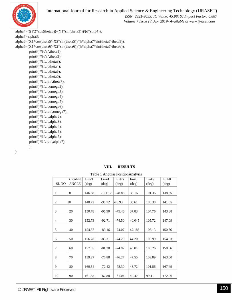
beta=165; thetakh=asin((c*sin(theta3-180))/h); theta7=thetakh+180; k7=((d*cos(theta4))+(i*cos(thetac))+(h*cos(theta7))); k8=((d*sin(theta4))+(i*sin(thetac))+(h*sin(theta7))); k9=((f*f-g*g-k7*k7-k8*k8)/(2*g)); G=k9+1; H=2; I=k9-1; theta61=2*atan((-H+sqrt((H*H)-(4*G*I)))/(2*G)); theta62=2*atan((-H-sqrt((H*H)-(4*G*I)))/(2*G)); if(theta61>0) theta6=theta61; else if(theta62>0) theta6=theta62; k10=(((g*g)-(f*f)-(k7*k7)-(k8*k8))/(2*f)); J=k10+1; K=2; L=k10-1; theta51=2*atan((-K+sqrt((K*K)-(4*J*L)))/(2*J)); theta52=2*atan((-K-sqrt((K*K)-(4*J*L)))/(2*J)); if(theta51>0) theta5=theta51; else if(theta52>0) theta5=theta52; omega2=20; sin24=((sin(theta2)*cos(theta4))-(cos(theta2)*sin(theta4))); sin34=((sin(theta3)*cos(theta4))-(cos(theta3)*sin(theta4))); omega3=((b*omega2*sin24)/(c*sin34)); sin32=((sin(theta3)*cos(theta2))-(cos(theta3)*sin(theta2))); sin43=((sin(theta4)*cos(theta3))-(cos(theta4)*sin(theta3))); omega4=(b*omega2*sin32)/(c*sin43); thetadf=acos (((f*f)+(d*d)-(e*e))/(2*f*d)); thetac=thetadf+15; beta=165; thetajh=asin ((d*sin(beta))/j); theta7=thetajh+180; sin54=(sin(theta5)*cos(theta4))+(cos(theta5)*sin(theta4)); sin57=(sin(theta5)*cos(theta7))+(cos(theta5)*sin(theta7)); sin65=(sin(theta6)*cos(theta5))+(cos(theta6)*sin(theta5)); sin64=(sin(theta6)*cos(theta4))+(cos(theta6)*sin(theta4)); sin67=(sin(theta6)*cos(theta7))+(cos(theta6)*sin(theta7)); sin56=(sin(theta5)*cos(theta6))+(cos(theta5)*sin(theta6)); omega7=omega3; omega6=((d*omega4*sin54)+(h*omega7*sin57))/(g*sin65); omega5=((d*omega4*sin64+h*omega7*sin67))/(g*sin56); Y2=((b*omega2*omega2*cos(theta2))+(b*alpha2*sin(theta2))+(c*omega3*omega3*cos(theta3))+(d*omega3* omega3*cos(theta4))); Y1=((b*alpha2*cos(theta2))-(b*omega2*omega2*sin(theta2))-(c*omega3*omega3*sin(theta3))-(d*omega4*omega4*sin(theta4))); alpha3=(((Y2*cos(theta4))-(Y1*sin(theta4)))/(c*sin43));




alpha4=(((Y2*cos(theta3))-(Y1*sin(theta3)))/(d*sin34)); alpha7=alpha3; alpha6=(X1*cos(theta5)-X2*sin(theta5))/(h*alpha7*sin(theta7-theta5)); alpha5=(X1*cos(theta6)-X2*sin(theta6))/(h*alpha7*sin(theta7-theta6)); printf("%d\t",theta1); printf("%d\t",theta2); printf("%f\t",theta3); printf("%f\t",theta4); printf("%f\t",theta5); printf("%f\t",theta6); printf("%f\n\n",theta7);

printf("%f\t",omega2); printf("%f\t",omega3); printf("%f\t",omega4); printf("%f\t",omega5); printf("%f\t",omega6); printf("%f\n\n",omega7); printf("%f\t",alpha2); printf("%f\t",alpha3); printf("%f\t",alpha4); printf("%f\t",alpha5); printf("%f\t",alpha6); printf("%f\n\n",alpha7); } }

VIII. RESULTS

Table 1 Angular PositionAnalysis

SL NO CRANK ANGLE

Link3 (deg)

Link4 (deg)

Link5 (deg)

link6 (deg)

Link7 (deg)

Link8 (deg)

1

0

146.58

-101.12

-78.88

33.16

101.36

138.65

2

10

148.72

-98.72

-76.93

35.61

103.30

141.05

3

20

150.78

-95.90

-75.46

37.83

104.76

143.88

4

30

152.73

-92.71

-74.50

40.045

105.72

147.09

5

40

154.57

-89.16

-74.07

42.186

106.13

150.66

6

50

156.28

-85.31

-74.20

44.20

105.99

154.53

7

60

157.85

-81.20

-74.92

46.018

105.26

158.66

8

70

159.27

-76.88

-76.27

47.55

103.89

163.00

9

80

160.54

-72.42

-78.30

48.72

101.86

167.49

10

90

161.65

-67.88

-81.04

49.42

99.11

172.06




Table 2 Angular Velocity Analysis

Table 3 Angular Acceleration Analysis SL.NO

CRANK ANGLE

link3

(rad/s2)

link4

(rad/s2)

link5

(rad/s2)

link6

(rad/s2)

link7

(rad/s2)

link8

(rad/s2) 1 0 -30.10 232.18 -232.18 30.10 -234.81 235.97

2

10

-43.43 216.31 -246.68 13.06 -249.09 219.86

3

20

-53.54 198.67 -260.38 -8.16 -262.23 201.59

4

30

-61.04 179.05 -274.06 -33.96 -275.17 181.15

5

40

-66.60 157.29 -288.64 -64.74 -289.02 158.60

6

50

-70.95 133.23 -305.08 -100.88 -304.85 133.92

7

60

-74.92 106.56 -324.25 -142.77 -323.59 106.84

8

70

-79.42 76.64 -346.73 -190.66 -345.75 76.74

9

80

-85.55 42.35 -372.36 -244.45 -371.15 42.45

10

90

-94.66 1.80 -399.65 -303.18 -398.25 2.05

Figure 21 Assembly of fabricated parts

SL NO

CRANK ANGLE

Link 3 (rad/s)

Link 4 (rad/s)

link 5 (rad/s)

Link 6 (rad/s)

Link 7 (rad/s)

Link 8 (rad/s)

1 0 6.525822 6.525822 6.525822 6.525822 6.525822 6.525822 2 10 6.310215 7.831239 5.132296 6.65332 5.117425 7.852798 3 20 6.026708 9.039326 3.657079 6.669697 3.629663 9.07983 4 30 5.692273 10.13911 2.102629 6.549462 2.06655 10.19423 5 40 5.3202 11.11857 0.466455 6.264823 0.426057 11.18353 6 50 4.919673 11.96486 -1.25948 5.785712 -1.30027 12.03552 7 60 4.49535 12.66379 -3.08864 5.079794 -3.12678 12.73717 8 70 4.046858 13.19849 -5.03884 4.1128 -5.07213 13.2729 9 80 3.568034 13.54713 -7.12927 2.849825 -7.15619 13.62204 10 90 3.045643 13.67923 -9.37485 1.258737 -9.39418 13.75507




IX. CONCLUSIONS

A. In this project design, kinematic and fabrication using 3d printing technology is performed. B. Equations are derived for position, angular velocity and angular acceleration of every link of Klann linkage using complex

algebraic method. C. a c-code is written for the calculations obtained using complex algebraic method. D. A 4 legged model of walking mechanism whose legs are based on Klann mechanism is designed using solid works. E. The different parts of the walking mechanism are 3d printed using PLA material for the selected dimensions.

REFERENCES [1] Aan and M. Heinloo “Analysis and synthesis of the walking linkage of Theo Jansen with a flywheel” [2] Hyun Gyu Kim , JaeNeung Choi ,TaeWon Seo and Kyungmin Jeong “Optimal Design of Klann-based Walking Mechanism for Water-running Robots” [3] Jaichandar Kulandaidaasan Sheba ; Edgar Martínez-García ; Mohan Rajesh Elara ; Le Tan-Phuc. (ICICS 2015) [4] Kim, Hyun-Gyu;Jung, Min-Suck;Shin, Jae-Kyun;Seo, TaeWon.”Optimal Design of Klann-linkage based Walking Mechanism for Amphibious Locomotion on

Water and Ground”.(Journal of Institute of Control, Robotics and Systems 2014.09.01) [5] Madugula Jagadeesh , Y V Chaitanya Kumar and Reddipalli Revathi “Design and optimization of a one-degree-of-freedom six- bar

linkage Klann mechanism” [6] Shunsuke Nansaia, Mohan Rajesh Elarab, Masami Iwase. “Dynamic Analysis and Modeling of Jansen Mechanism”.(Elseviser 2013) [7] V. V. Pharate, S. M. Patil, O. M. Prajapati, S. P. Patil. “Kinematic Synthesis And Optimum Selection Of Planar Straight Line Mechanism”.(IOSR-JMCE)

7 IV April 2019

Documents

Transcript of 7 IV April 2019