40 CFR 51.300 and Appendi - Environmental Protection Division
77
Exemption Modeling Analysis in Support of the Best Available Retrofit Technology (BART) Regulations - 40 CFR 51.300 and Appendix Y Prepared for: International Paper Augusta Mill 4278 Mike Padgett Highway Augusta, GA 30906 Prepared by: URS Corporation – North Carolina 1600 Perimeter Park Drive, Suite 400 Morrisville, North Carolina 27560 July 28, 2006
-
Upload
khangminh22 -
Category
Documents
-
view
2 -
download
0
Transcript of 40 CFR 51.300 and Appendi - Environmental Protection Division
Exemption Modeling Analysis in Support of the Best Available Retrofit Technology (BART) Regulations - 40 CFR 51.300 and Appendix Y Prepared for:
International Paper Augusta Mill 4278 Mike Padgett Highway Augusta, GA 30906 Prepared by:
URS Corporation – North Carolina 1600 Perimeter Park Drive, Suite 400 Morrisville, North Carolina 27560 July 28, 2006
Exemption Modeling Analysis in Support of the
Best Available Retrofit Technology (BART) Regulations - 40 CFR 51.300 and Appendix Y
International Paper Augusta, Georgia
Prepared for: International Paper – Augusta Mill
4278 Mike Padgett Highway Augusta, Georgia 30906
Prepared by: URS Corporation – North Carolina
1600 Perimeter Park Drive, Suite 400 Morrisville, North Carolina 27560
July 28, 2006
ii
Table of Contents Page
1.0 Introduction and Background ......................................................................................... 1 1.1 Objective of BART Exemption Modeling.............................................................. 3 1.2 Response to Protocol Comments ............................................................................ 4 1.3 Facility Location and Relevant Class I Areas......................................................... 5 1.4 Source Impact Evaluation Criteria.......................................................................... 7 1.5 General Overview of the CALPUFF Modeling System......................................... 7
2.0 BART Source Descriptions .............................................................................................. 7 2.1 Unit Specific Source Data....................................................................................... 7 2.2 Tabulated Source Data.......................................................................................... 10
3.0 Geophysical and Meteorological Data .......................................................................... 12
4.0 CALPUFF Modeling Methodology ............................................................................... 12 4.1 Methodology......................................................................................................... 12 4.2 CALMET Model Configuration and Application................................................. 12 4.3 CALPUFF Model Configuration and Application ............................................... 13
4.3.1 Domain Definition................................................................................... 13 4.3.2 Model Set-Up .......................................................................................... 15 4.3.3 Emissions Input Development................................................................. 15 4.3.4 Additional CALPUFF Input Information and Settings ........................... 15
5.0 POSTUTIL PROCESSING ........................................................................................... 16
6.0 CALPOST PROCESSING............................................................................................. 16 6.1 Visibility Assessment............................................................................................ 17
7.0 REPORTING .................................................................................................................. 19 7.1 CALPUFF Modeling Results................................................................................ 19
8.0 REFERENCES................................................................................................................ 23 Appendices Appendix A Emission Rates and Supporting Information Appendix B CALFUFF Configuration Appendix C CALPOST Configuration Appendix D Class I Receptors in Lambert Conformal Coordinates
iii
List of Tables Page
Table 2-1 BART Eligible Emission Units - Point Source Parameters .................................. 10 Table 2-2 BART Eligible Emission Units - Volume Source Parameters.............................. 11 Table 6-1 Default Natural Background Concentrations (µg/m3) for Eastern U.S.
Class I Areas (Source: EPA, 2003, Table 2-1).................................................. 19 Table 7-1 BART Exemption Modeling Results for Eight Class I Areas .............................. 20 Table 7-2 Summary of BART Exemption Modeling Results - Three-Year Approach......... 22
List of Figures Figure 1-1 Facility Location Relative to Class I Areas ............................................................ 6 Figure 4-1 VISTAS CALMET DOMAIN with CALPUFF Sub-domain ............................ 14
Executive Summary
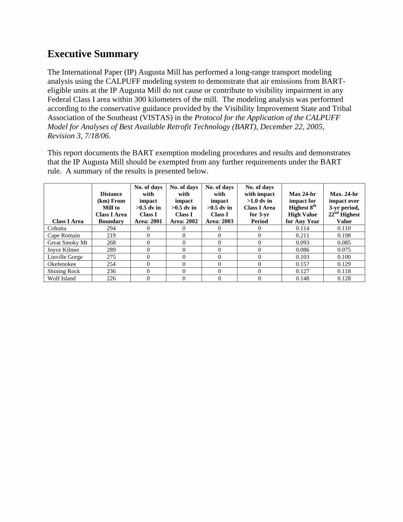
The International Paper (IP) Augusta Mill has performed a long-range transport modeling analysis using the CALPUFF modeling system to demonstrate that air emissions from BART-eligible units at the IP Augusta Mill do not cause or contribute to visibility impairment in any Federal Class I area within 300 kilometers of the mill. The modeling analysis was performed according to the conservative guidance provided by the Visibility Improvement State and Tribal Association of the Southeast (VISTAS) in the Protocol for the Application of the CALPUFF Model for Analyses of Best Available Retrofit Technology (BART), December 22, 2005, Revision 3, 7/18/06.
This report documents the BART exemption modeling procedures and results and demonstrates that the IP Augusta Mill should be exempted from any further requirements under the BART rule. A summary of the results is presented below.
Class I Area
Distance (km) From
Mill to Class I Area Boundary
No. of days with
impact >0.5 dv in
Class I Area: 2001
No. of days with
impact >0.5 dv in
Class I Area: 2002
No. of days with
impact >0.5 dv in
Class I Area: 2003
No. of days with impact >1.0 dv in
Class I Area for 3-yr Period
Max 24-hr impact for Highest 8th High Value
for Any Year
Max. 24-hr impact over 3-yr period, 22nd Highest
Value Cohutta 294 0 0 0 0 0.114 0.110 Cape Romain 219 0 0 0 0 0.211 0.198 Great Smoky Mt 268 0 0 0 0 0.093 0.085 Joyce Kilmer 289 0 0 0 0 0.086 0.075 Linville Gorge 275 0 0 0 0 0.103 0.100 Okefenokee 254 0 0 0 0 0.157 0.129 Shining Rock 236 0 0 0 0 0.127 0.118 Wolf Island 226 0 0 0 0 0.148 0.128
1
1.0 Introduction and Background
International Paper (IP) has retained URS Corporation (URS) to assist in the development of a long-range transport modeling analysis using the CALPUFF modeling system to demonstrate that air emissions from BART eligible units at the IP Augusta Mill do not cause or contribute to visibility impairment in any Federal Class I area within 300 kilometers of the mill. These regulatory modeling requirements are briefly defined in 40 CFR 51, Appendix Y. The modeling was conducted using the detailed procedures outlined in a common protocol developed by the Visibility Improvement State and Tribal Association of the Southeast (VISTAS) and a “site-specific” protocol developed by URS and submitted to the Georgia Department of Natural Resources, Environmental Protection Division (Georgia DNR) on April 28, 2006.
Comments and recommendations from Georgia DNR on the “site-specific” protocol have been incorporated into this modeling analysis. The following provides a regulatory background of the BART regulation and summarizes the modeling procedures used to conduct the BART exemption modeling.
The Clean Air Act established goals for visibility in many national parks and wilderness areas. Through the 1977 amendments to the Clean Air Act, Congress set a national goal for visibility as “the prevention of any future, and the remedying of any existing, impairment of visibility in mandatory Class I Federal areas which impairment results from manmade air pollution.” The Amendments required EPA to issue regulations to assure “reasonable progress” toward meeting the national goal.
In 1980, EPA promulgated regulations to address the visibility impairment that is “reasonably attributable” to a single source or small group of sources. In 1988, the States, Federal Land Managers (e.g., National Park Service, U.S. Forest Service, U.S. Fish and Wildlife Service, Bureau of Land Management), and EPA began monitoring of fine particle concentrations and visibility in 30 national parks and wilderness areas across the country.
The Clean Air Act Amendments of 1990 required EPA to take regulatory action on regional haze and they proposed the Regional Haze Regulations in July 1997 in conjunction with issuing new national ambient air quality standards for fine particulate matter.
On July 1, 1999, EPA promulgated the final Regional Haze Regulation. The final Regional Haze Regulation calls for state and federal agencies to work together to improve visibility in 156 national parks and wilderness areas in the United States by developing and implementing long-term air quality protection plans to reduce the pollution that causes visibility impairment in these protected areas.
The Regional Haze regulation provides States flexibility in determining reasonable progress goals for protected areas by conducting certain analyses to ensure that they consider the possibility of setting an ambitious reasonable progress goal, one that is aimed at reaching natural background conditions by the year 2064. The regulation requires States to establish goals for each affected area to (1) improve visibility on the haziest days, and (2) ensure no degradation occurs on the clearest days over the period of each implementation plan.
2
The Regional Haze regulation also requires States to develop long-term strategies including enforceable measures designed to meet reasonable progress goals. The first long-term strategy will cover 10 to 15 years, with reassessment and revision of those goals and strategies in 2018 and every 10 years thereafter. State’s strategies will address their contribution to visibility problems in Class I areas both within and outside the State.
One of the principal elements of the visibility protection provisions of the Clean Air Act addresses installation of best available retrofit technology (BART) for certain existing sources. “BART-eligible” sources are those sources built between 1962 and 1977 that have the potential to emit more than 250 tons per year of one or more visibility-impairing compounds including sulfur dioxide (SO2), nitrogen oxides (NOx), particulate matter (PM), and volatile organic compounds (VOCs), and that fall within 26 industrial source categories (including Kraft pulp and paper manufacturing).
Soon after the Regional Haze Regulation was finalized, several parties filed petitions to challenge the rule with the U.S. Court of Appeals for the D.C. Circuit. In April 2004, EPA Administrator Mike Leavitt signed a proposed amendment to the 1999 Regional Haze Regulation. The proposed rule satisfied the terms of a May 2002 ruling by the U.S. Court of Appeals for the D.C. Circuit, which vacated parts of the BART provisions of the 1999 Regional Haze Regulation (American Corn Growers et. al. v. EPA, 291 F. 3d 1 (D.C. cir. 2002)).
The rule requires states to consider the visibility impacts of an individual facility when determining whether they have to install controls. The final BART implementation and guidance rule (40 CFR Part 51, Appendix Y) was published on July 6, 2005 and it allows for a BART evaluation for any BART-eligible source that “emits any air pollutant which may reasonably be anticipated to cause or contribute to any impairment of visibility” in any mandatory Class I federal area.
Pursuant to the rule, States have the option of exempting a BART-eligible source from the BART requirements based on dispersion modeling demonstrating that the source cannot reasonably be anticipated to cause or contribute to visibility impairment in a Class I area. Regional Planning Organizations (RPOs), such as the VISTAS have prepared guidance for performing the dispersion modeling analyses. According to 40 CFR Part 51, Appendix Y, a BART-eligible source is considered to “contribute” to visibility impairment in a Class I area if the modeled 98th percentile change in dv is equal to or greater than the “contribution threshold.” Any BART-eligible source determined to cause or contribute to visibility impairment in any Class I area is subject to a BART evaluation.
The Protocol for the Application of the CALPUFF Model for Analyses of Best Available Retrofit Technology (BART), December 22, 2005, Revision 3, 7/18/06, was prepared by the VISTAS RPO to provide some common guidance for performing conservative BART exemption and determination modeling evaluations as allowed by the regulation.
The final BART rule defines a “contribution threshold” of 0.5 dv as the value where a modeled BART eligible source may “contribute” to visibility impairment and the threshold to determine whether a single source “causes” visibility impairment is set at a 1.0-dv change from natural conditions (background visual range) over a 24-hour averaging period in the final BART rule (70
3
FR 39118). An approximate 1.0 deciview change was defined by Pitchford and Malm (1992) as a “just noticeable change” to the observer when the background visual range equals the line-of-sight (LOS) of the observer. According to L. Willard Richards in “Use of the Deciview Haze Index as an Indicator for Regional Haze” if a shorter LOS distance than the background visual range (natural conditions) is used in performing the calculations then a higher extinction value, or deciview, is needed to cause a “just noticeable change.” In other words, when the LOS is less than the background visual range, then it would require a higher deciview value in order to be a “just noticeable change.” Since large concentration gradients are expected when modeling single sources, it is generally understood that “single-source” visibility impairment modeling include some estimate of the change in concentration with distance. However, this is not done using current VISTAS modeling guidance.
The exemption modeling results presented in this report only use the conservative modeling approach as defined by the VISTAS protocol by determining the change in extinction at single maximum receptors in a Class I area and did not use the a refined modeling line-of-sight or sight path approach that is consistent with the definition of the deciview metric. This was done since the more conservative VISTAS modeling results produced values below levels of concern at each Class I area and the extra time and effort to do LOS modeling would provide little added value to the BART exemption analysis.
1.1 Objective of BART Exemption Modeling The objective of this BART exemption modeling analysis is to demonstrate that all BART eligible emission units located at the IP Augusta Mill do not cause or contribute to visibility impairment in any of the Class I areas located within 300 kilometers of the plant site. The VISTAS organization has developed a set of modeling procedures that were used to conduct the exemption modeling. These modeling procedures are discussed in the VISTAS document titled; Protocol for the Application of the CALPUFF Model for Analyses of Best Available Retrofit Technology (BART), December 22, 2005- Revision 3 – 7/18/06. The VISTAS modeling procedures and additional refinements are also discussed in a “site-specific” protocol developed by URS titled; Protocol for the Application of the CALPUFF Model in Support of the Best Available Retrofit Technology (BART) Regulations – 40 CFR 51.300 and Appendix Y, April 28, 2006. The VISTAS States, including Georgia, have accepted EPA’s guidance to use the CALPUFF modeling system to comply with the BART modeling requirements of the regional haze rule.
International Paper has conducted refined CALPUFF modeling to quantify the estimated visibility impairment of the mill’s BART-eligible emission units as compared to natural visibility conditions. The refined modeling procedures are discussed in this summary report. International Paper requests that the GA DNR review this report and provide IP with a notification letter stating that the BART exemption request has been approved based on the technical accuracy of the modeling approaches used therein. International Paper and URS Corporation are willing to discuss these model results in greater detail at any time with the Georgia DNR and supply any additional material needed in order to facilitate the review.
4
1.2 Response to Protocol Comments The Georgia DNR provided comments to IP Augusta regarding the site-specific BART exemption modeling protocol on June 23, 2006. The following items respond to the June 1, 2006 General Comments for all Georgia BART exemption Modeling Protocols from the US EPA.
Item 1. Rayleigh Scattering and Sea Salt: An adjusted Rayleigh Scattering and the use of a sea salt adjustment factor is a reasonable assumption that is based on good science. However, to expedite the review process, URS did not include any adjustments for Rayleigh Scattering and sea salts in this analysis. Item 2. GEP Stack Height: No IP Augusta BART eligible unit has a height greater than 65 meters; therefore, this issue does not impact the IP Augusta Mill. Item 3. a: Input modeling tables are being provided in this report which include all the recommended EPA model settings. b: We have included the basis for the determination of all BART eligible units. c: Comment not applicable to IP Augusta. Specific EPA Comments on the IP Augusta Mill are addressed below. 1. Use of 98th percentile for visibility threshold comparison. URS did not conduct any screening level CALPUFF modeling. Only refined 4-km modeling was performed, which allows the use of 98th percentile values. Final modeling results are based on the 98th percentile value for three individual years and three years combined. 2. AERMOD Turbulence-based dispersion. Standard Pasquill-Gifford (P-G) curves were used for this BART exemption modeling. 3. Ammonia-Limiting Method: As recommended by the Georgia DNR in the June 23, 2006 protocol comment letter under item 2, a value of 0.5 ppb for background ammonia was used for all modeling. 4. Alternative methodologies when VISTAS BART Protocol method fails. a. Sea Salt and Rayleigh Scattering Adjustments. URS did not make adjustments to the standard IMPROVE equation in this modeling submittal. b. Line-of-sight (LOS). The LOS approach was not used in this modeling analysis. c. URS believes that applying Method 7 or 7 prime would remove yet another conservative component from the BART modeling process. However, URS did not conduct any Method 7 or 7 prime modeling for this analysis. d. URS conducted all BART modeling for this analysis using the recommended VISTAS model procedures. These standard procedures are discussed in the reminder of this report.
5
The following items address the comments in the May 18, 2006 letter from the United States Department of Agriculture, Forest Service (FS) to Georgia Department of Natural Resources, Environmental Protection Division.
With respect to the FS comment on 12 kilometer screening procedures please refer to the URS response to the US EPA under specific item 1. With respect to the FS comment on the use of ammonia data please refer to the URS response to the US EPA under specific item 3. LOS modeling technique: LOS was not used in this modeling analysis. Method 7: URS did not use Method 7 modeling assumptions in this analysis. Relative Humidity, f(RH) and EPRI Coefficients: URS did not use any of these adjustments in this analysis. This BART exemption modeling analysis was conducted using standard (VISTAS) recommended modeling procedures. These procedures are discussed in the remainder of this report.
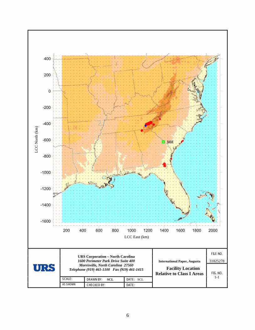
1.3 Facility Location and Relevant Class I Areas The International Paper Augusta, Georgia pulp and paper mill is located at 4278 Mike Padgett Highway near Augusta, Georgia. The Universal Transverse Mercator (UTM) coordinates, in kilometers (km), for the mill are Zone 17, 411.300 East and 3688.200 North. The approximate Lambert Conformal Conic (LCC) coordinates are 1390.566 km East and -623.286 km North. There are eight (8) Class I areas within 300 kilometers of the Augusta Mill: Cape Romain, Okefenokee and Wolf Island National Wildlife Refuge Areas, Shining Rock, Linville Gorge, Joyce Kilmer/Slickrock and Cohutta Wilderness Areas and the Great Smoky Mountains National Park. Figure 1-1 displays the location of the mill and the eight Class I areas. Cape Romain is located approximately 219 kilometers east of the mill, Wolf Island is located approximately 226 kilometers southeast of the mill, Okefenokee is located 254 kilometers south of the mill, Shining Rock is located 236 km northwest of the mill, Great Smoky Mountains is located 268 kilometers northwest of the mill, Linville Gorge is located 275 kilometers north of the mill, Joyce Kilmer/Slickrock is located 289 kilometers northwest of the mill and Cohutta is located 294 kilometers northwest of the mill.
6
200 400 600 800 1000 1200 1400 1600 1800 2000LCC East (km)
-1600
-1400
-1200
-1000
-800
-600
-400
-200
0
200
400
LCC
Nor
th (k
m)
Mill
FILE NO. 31825278
URS Corporation – North Carolina 1600 Perimeter Park Drive Suite 400 Morrisville, North Carolina 27560
Telephone (919) 461-1100 Fax (919) 461-1415
SCALE: DRAWN BY: SCL DATE: SCL
AS SHOWN CHECKED BY: DATE:
International Paper, Augusta
1-2 Facility Location Relative to Class I Areas FIG. NO.
1-1
7
1.4 Source Impact Evaluation Criteria To assess whether a BART eligible source is exempt from performing a BART control technology evaluation, a two-tiered modeling approach is suggested by VISTAS: a screening level analysis which uses 12-km grid data from CALMET with no supporting observational data included or a more refined CALMET data with a grid spacing of 4-km with observational data to better define a facilities impact. In order to perform the exemption modeling in the most efficient manner, URS has skipped the screening level modeling analysis using the 12-km grid data and has only used the 4-km refined meteorological data. Using the 4-km data provides a more accurate prediction of the mill’s impact on visibility as compared to natural conditions.
As suggested in VISTAS BART modeling guidance, the CALPUFF/CALPOST models were used to estimate a maximum 98th percentile value for visibility impairment during a 24-hour averaging period. The higher of the 8th highest individual year or the 22nd highest for the three-year modeling period are reported. This value was compared to the EPA/VISTAS recommended visibility threshold of 0.5 dv.
1.5 General Overview of the CALPUFF Modeling System The CALPUFF modeling system consists of three main processors: CALMET, CALPUFF and CALPOST. CALMET is the meteorological model that generates hourly three-dimensional meteorological fields of variables such as wind and temperature. CALPUFF simulates the transport, dispersion, and transformation of compounds emitted from a source and calculates hourly concentration values for visibility impairing compounds at each receptor located in the modeling domain. CALPOST calculates time-averaged concentration values from the CALPUFF predictions and performs regional haze calculations like those described in the Section 6.1 of this report.
2.0 BART Source Descriptions
The IP Augusta Mill is located near Augusta, Georgia, along the Savannah River. The primary activities at Augusta Mill are pulp production (Standard Industrial Classification [SIC] code 2611) and paperboard production (SIC code 2631). The Mill began operations in 1960. Primary operations at the mill include multiple fuel-fired boilers, chemical recovery operations, wood pulping and bleaching operations, papermaking, and additional operations and equipment necessary to support these operations. The facility currently employs about 750 people, and produces a nominal 750,000 tons per year of coated bleached board used for greeting cards, pharmaceutical and foodservice packaging, and cigarette packaging.
2.1 Unit Specific Source Data The emission estimates used in the CALPUFF model are intended to reflect steady-state operating conditions during periods of high capacity utilization. Consistent with the VISTAS common protocol, modeled emissions do not include periods of start-up, shutdown, and malfunction. The modeling is based on the 24-hour average actual emission rate from the highest emitting day during the most recent 3-year period. The following hierarchy for developing the emission estimates was used for the IP Augusta mill:
8
• Continuous Emissions Monitoring (CEM) data; • Facility emissions tests; • Emission factors; • Permit limits; or • Potential to emit.
The Augusta Mill developed emission estimates based on source testing and accepted emission factors used for routine annual emissions reporting. In general, the following emission rates were used:
• Short-term (24-hours) allowable emission rates (e.g., emission rates calculated using the maximum rated capacity of the source);
• Federally enforceable short-term limits (24-hours); or • Peak 24-hour actual emission rates (or calculated emission rates) from the most
recent 3-years of operation that account for “high capacity utilization” during normal operating conditions and fuel/material flexibility allowed under the existing air permit. In situations where a unit is allowed to use more than one fuel, the fuel resulting in the highest emission rates was used for the modeling, as long as that fuel represented a realistic 24-hour operating scenario. Scenarios representing periods of startup, shutdown, or malfunction were not modeled.
Short-term emission rates (24-hours) for SO2, NOx, H2SO4 mist, and PM10 (including condensable and filterable direct PM10) were modeled since visibility changes are calculated for a 24-hour averaging period. All BART-eligible emission units at the mill that emit these compounds were modeled together in the CALPUFF model. Listed below is a brief description of all the BART-eligible emission units at the mill:
• No. 2 Power Boiler (PB2A): This boiler fires pulverized coal, No. 6 fuel oil, natural gas, and used oil. The No. 2 Power Boiler also serves as a backup control device for the non-condensable gas (NCG) system. The No. 2 Power Boiler nominal throughput is 532 MMBtu/hr when firing pulverized coal, 600 MMBtu/hr when firing No. 6 fuel oil, and 677 MMBtu/hr when firing natural gas. The unit is controlled by an electrostatic precipitator.
• No. 2 Recovery Boiler (RB2A): This direct contact evaporator (DCE) recovery boiler fires black liquor solids, with No. 6 fuel oil or natural gas as auxiliary fuels. The No. 2 Recovery Boiler nominal throughput is 2.0 million pounds of black liquor solids per day, 460 MMBtu/hr when firing No. 6 fuel oil during periods of SSM or low BLS throughput, and 100 MMBtu/hr of natural gas. The unit is controlled by an electrostatic precipitator.
• No. 2 Smelt Dissolving Tank (ST2A): This smelt dissolving tank receives smelt from the No. 2 Recovery Boiler. This unit is controlled by a wet scrubber.
• No. 2 Paper Machine (PM2A): This paper machine is equipped with 28 infrared (IR) heaters (1.1 MMBtu/hr each) and 2 aircap heaters (rated at 3.4 and 8.0 MMBtu/hr) that are natural gas fired.
9
• No. 1 Slaker/Causticizer (CAU1): The No. 1 Slaker/Causticizer has a maximum throughput of 13 tons CaO per hour. The slaker vent duct is equipped with a liquid spray nozzle, but this is not considered a formal air pollution control device.
The following BART-eligible units do not emit SO2, NOx, H2SO4 mist, or PM10 and were not modeled.
• No. 2 A/B Filtrate Tank (2ABF) • No. 2 Brownstock Washer and Screens (BSW2) • No. 2 Evaporators (EV2A) • No. 2 Green Liquor Clarifier (GLC2) • No. 1 Black Liquor Pond (BLP1) – Closed in 2006
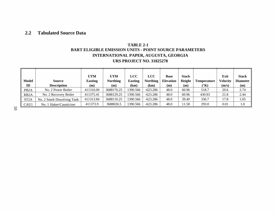
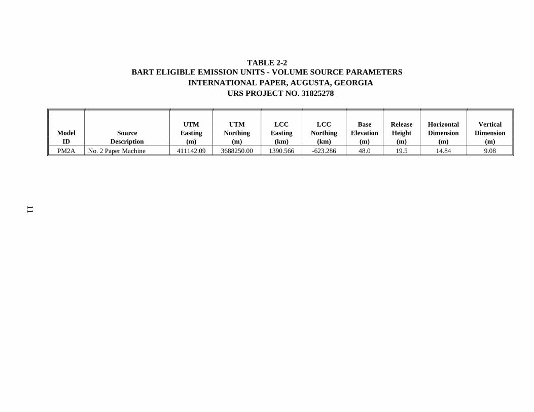
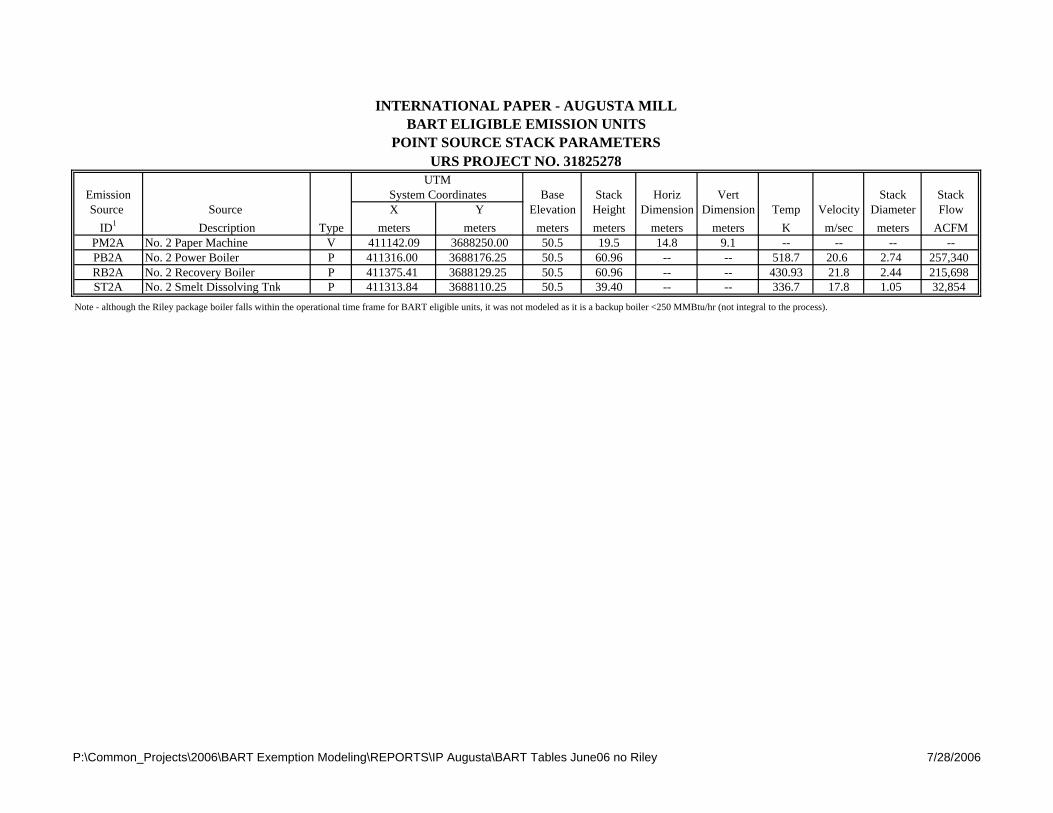
The Riley Auxiliary Boiler (RLYA) was recently excluded from the list of BART-eligible emission units because it is a backup boiler with heat input less than 250 MMBtu. It is not integral to the process. The Riley Auxiliary Boiler fires No. 2 fuel oil or natural gas and is permitted to operate only when one of the primary boilers or recovery boilers is offline. The Riley Boiler’s nominal throughput is 220 MMBtu/hr. Appendix A provides information on how the list of BART-eligible units was developed and presents the emission rate calculations for the BART-eligible units that emit SO2, NOx, H2SO4 mist, or PM10. Tables 2-1 and 2-2 provide detailed stack parameter information for the modeled BART-eligible emission units at the mill.
10
2.2 Tabulated Source Data
TABLE 2-1 BART ELIGIBLE EMISSION UNITS - POINT SOURCE PARAMETERS
INTERNATIONAL PAPER, AUGUSTA, GEORGIA URS PROJECT NO. 31825278
UTM UTM LCC LCC Base Stack Exit Stack
Model Source Easting Northing Easting Northing Elevation Height Temperature Velocity Diameter ID Description (m) (m) (km) (km) (m) (m) (°K) (m/s) (m)
PB2A No. 2 Power Boiler 411316.00 3688176.25 1390.566 -623.286 48.0 60.96 518.7 20.6 2.74 RB2A No. 2 Recovery Boiler 411375.41 3688129.25 1390.566 -623.286 48.0 60.96 430.93 21.8 2.44 ST2A No. 2 Smelt Dissolving Tank 411313.84 3688110.25 1390.566 -623.286 48.0 39.40 336.7 17.8 1.05 CAU1 No. 1 Slaker/Causticizer 411373.9 3688026.5 1390.566 -623.286 48.0 11.58 293.0 0.01 1.0
11
TABLE 2-2 BART ELIGIBLE EMISSION UNITS - VOLUME SOURCE PARAMETERS
INTERNATIONAL PAPER, AUGUSTA, GEORGIA URS PROJECT NO. 31825278
UTM UTM LCC LCC Base Release Horizontal Vertical
Model Source Easting Northing Easting Northing Elevation Height Dimension Dimension ID Description (m) (m) (km) (km) (m) (m) (m) (m)
PM2A No. 2 Paper Machine 411142.09 3688250.00 1390.566 -623.286 48.0 19.5 14.84 9.08
12
3.0 Geophysical and Meteorological Data
URS used the geophysical and meteorological data developed by VISTAS for the 4-km BART exemption modeling. The development of this information was discussed in detail in the VISTAS common protocol.
4.0 CALPUFF Modeling Methodology
CALPUFF modeling was conducted using the 4-km data in order to efficiently and more accurately demonstrate that the IP Augusta Mill does not cause or contribute to visibility impairment in any Class I area and thus is exempt from the BART rule. The modeling methods described in this section were used to identify specific Class I areas that might be most affected by emissions from the BART eligible emission units located at the IP Augusta Mill. It needs to be noted that the CALPUFF modeling used all recommended data that was publicly available on April 1, 2006. Background concentrations for SO4 and TNO3 from CMAQ (2001-2003) annual runs were not publicly available on that date; therefore, URS could not include this information in the CALPUFF runs and still meet Georgia DNR submittal deadlines.
CALPUFF modeling was performed using the standard set of default meteorological, air quality and dispersion conditions that have been developed by VISTAS for the 4-km gridded CALMET domain number five. It is our understanding that these data were developed to be consistent with recommendations developed by the Interagency Workgroup on Air Quality Modeling (IWAQM, 1998) and FLAG (2000).
4.1 Methodology This analysis was performed using the CALPUFF model with three years of meteorological data developed by VISTAS along with the standard compliment of model algorithms invoked. URS evaluated the 98th percentile impacts since 4-km data is being used for the analysis and this percentile is recommended under 40 CFR 51, Appendix Y.
The regional haze impacts at each applicable Class I area were calculated from the daily visibility values for each receptor by determining the change in deciviews compared against natural visibility conditions. EPA’s “Guidance for Estimating Natural Visibility Conditions Under the Regional Haze Rule,” EPA-454/B03-005 (September 2003) lists recommended natural visibility conditions. To determine whether IP Augusta may reasonably be anticipated to cause or contribute to visibility impairment at a nearby Class I area, the impacts predicted by CALPUFF were compared against the pertinent natural visibility background and the threshold that has been selected.
4.2 CALMET Model Configuration and Application Sections 4.3.2 and 4.4.2 within the VISTAS common protocol discuss in detail the model configurations used to generate the common CALMET meteorological files for modeling BART eligible sources. The configuration is reported to follow the IWAQM recommendations (EPA, 1998, Appendix A), except as noted in the protocol. For CALPUFF modeling there is no need to compile CALMET inputs, run the CALMET model or evaluate the outputs.
13
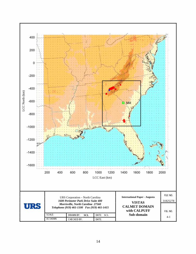
The model-ready meteorological data sets have been developed by VISTAS for one large regional domain and five smaller sub-regional domains. The IP Augusta Mill is located in sub-regional domain number 4 depicted in the VISTAS common protocol. Figure 4-1 displays the configuration of the regional domain and the size and location of the smaller CALPUFF modeling domain used in the analysis.
4.3 CALPUFF Model Configuration and Application URS used the newly released VISTAS version of the CALPUFF modeling system version 5.754. This version contains enhancements funded by the Minerals Management Service (MMS) and VISTAS. This version includes CALMET, CALPUFF, CALPOST, CALSUM, POSTUTIL, and CALVIEW, and it was obtained from the CALPUFF website.
All CALPUFF modeling used the standard P-G curves. The sequence of model processors for all modeling was CALPUFF then CALPOST. POSTUTIL was not used to conduct ALM modeling since very little benefits (lower predicted concentrations) were seen from using the ALM procedures for this facility. POSTUTIL also was not used for particle size modeling since all particulate matter (PM) was assumed to be in the 0.48 micron category and this greatly speeded up the modeling process by being able to go directly from CALPUFF to CALPOST by simply defining the PM components in terms of coarse, soil, elemental carbon and secondary organic aerosol. Not using POSTUTIL for ALM or PM particle size modeling is a conservative process (may produce slightly higher impacts). Initial tests using POSTUTIL showed this to be the case. The total contribution to visibility impairment from PM emissions is relatively minor when compared to the contributions from nitrates and sulfates. This can be seen by examining the CALPOST output files. CALMET and associated preprocessors are not discussed since VISTAS performed these model runs.
4.3.1 Domain Definition The meteorological modeling data sets cover three contiguous years (2001, 2002, and 2003) and have been resolved to a 4-km horizontal resolution grid using MM5 data. Details of the modeling domains and the meteorological databases for 2001, 2002, and 2003 are discussed in detail in the VISTAS common protocol.
Receptor Network and Class I Receptors. Discrete receptor coordinate data for the eight Federal Class I areas within 300 km of the source were developed using the National Park Service (NPS) Convert Class I Areas (NCC) computer program. The receptor elevations provided by the NPS were used for modeling. All receptors for each Class I area were included in single CALPUFF simulations. There are 110 receptors listed for Shining Rock, 745 receptors for the Great Smoky Mountains, 66 receptors for Linville Gorge, 101 receptors for Joyce Kilmer/Slickrock 220 receptors for the Cohutta Class I area, 164 receptors for Cape Romain, 30 receptors for Wolf Island and 490 receptors for the Okefenokee Class I area. Appendix D contains a listing of the Lambert Conformal coordinates for each Class I area with the associated receptor heights.
14
200 400 600 800 1000 1200 1400 1600 1800 2000LCC East (km)
-1600
-1400
-1200
-1000
-800
-600
-400
-200
0
200
400
LCC
Nor
th (k
m)
Mill
FILE NO. 31825278
URS Corporation – North Carolina
1600 Perimeter Park Drive Suite 400 Morrisville, North Carolina 27560
Telephone (919) 461-1100 Fax (919) 461-1415 FIG. NO.
SCALE: DRAWN BY: SCL DATE: SCL
AS SHOWN CHECKED BY: DATE:
International Paper - Augusta
VISTAS CALMET DOMAIN
with CALPUFF Sub-domain
4-1
15
4.3.2 Model Set-Up The modeling used a CALPUFF computational domain that includes all applicable Class I areas within 300 km of the source and a 50-kilometer buffer around applicable Class I areas and the mill. The size and location of the 4-km CALPUFF computational domains is shown in Figure 4-1.
As depicted in Figure 4-1, the CALPUFF modeling domain is a subset of the larger regional and sub-regional CALMET meteorological domains. A smaller CALPUFF domain is being used to reduce the CALPUFF run times. The CALPUFF 4-km sub domain is approximately 612 km in the east/west direction and 684 km in the north/south direction. Using a 4-km grid spacing from the CALMET files, this would relate to 153 x 171 grid squares. Appendix B contains a summary of the input options selected when performing CALPUFF modeling.
4.3.3 Emissions Input Development Emissions from the facility include SO2, NOx, H2SO4 mist, and PM10 (including condensable and filterable in the form of coarse, soil, elemental carbon, and secondary organic aerosol PM).
Emissions Speciation. URS used the example spreadsheets supplied by VISTAS and the CMAQ speciation profiles available on EPA’s website for PM speciation. Appendix A provides detailed information on PM speciation for the BART-eligible units.
Condensable Emissions. Condensable emissions were considered primary fine particulate matter. Appendix A provides detailed information on condensable and filterable PM emissions from the BART-eligible units.
Size Classification of Primary PM Emissions. As a conservative modeling assumption all PM was modeled in the 0.48 micron category. This is due to the fact that the non-hygroscopic PM has a relatively minor impact on visibility impairment based information from CALPOST.
4.3.4 Additional CALPUFF Input Information and Settings CALPUFF Model Options. The model options, parameter settings, and ‘switches’ for exercising CALPUFF for BART modeling are discussed below. Appendix B contains tables that list the default and the actual modeled configurations used for the BART modeling. The default configurations are from the IWAQM Phase 2 Report (EPA, 1998).
Visibility Modeling Domain. The CALPUFF domain was configured to include the source and all Class I areas within 300 km. An additional 50-km buffer zone was established in each cardinal direction from the source and Class I area.
Building Downwash. Building and structure information was not included.
Puff Dispersion. Based on recent guidance from EPA and VISTAS the current default P-G dispersion curves were used for CALPUFF modeling.
Puff Representation. The default integrated puff sampling methodology was used in CALPUFF.
Puff Splitting. There is no quantitative evidence that the horizontal and vertical puff-splitting algorithms in CALPUFF yield improved accuracy and precision in model estimates of inert or

16
linearly reactive compounds although conceptually the methods are appealing because they mimic lateral and vertical wind speed and direction shears. Therefore puff splitting was not invoked.
Chemical Mechanism. The MESOPUFF II module was used for BART modeling. For the aqueous phase conversion of SO2 to sulfate (important when the plume interacts with clouds and fog), the IWAQM defaults were used, i.e., nighttime SO2 loss rate (RNITE1) is assumed to be 0.2 percent per hour. The nighttime NOx loss rate (RNITE2) and HNO3 formation rate (RNITE3) are both set to 2.0 percent per hour.
Particulate matter emissions by size category were combined into the appropriate species for the visibility analysis. These species include (a) elemental carbon (EC), (b) fine PM or “soil” (<2.5 µm in diameter), (c) coarse PM (between 2.5-10 µm in diameter), and (d) organics, referred to as secondary organic aerosols in the CALPOST postprocessor.
Background Ozone Concentrations. Ozone concentration data for 2001-2003 from ambient AIRS/CASNET monitors located within the particular domain being modeled were used to develop background estimates. Only non-urban ozone stations were used in the OZONE.DAT file. Monthly average ozone background values was computed for the Class I area that had the highest ozone measurements in the domain which was Shinning Rock. The values represent the daytime average ozone concentrations (6 am to 6 pm average).
Background Ammonia Concentrations. A constant (0.5 ppb) value was used for ammonia.
Other Background Concentrations. Concentrations of SO4 and TNO3 (HNO3 + NO3) from CMAQ 2001-2003 were not made available in time to be included in the modeling submittal. In a borderline modeling situation this could be an important component. However, the current modeling results indicate that this data would need to have a major impact to change the conclusions given in this report. Georgia DNR or VISTAS may wish to include this data for completeness after the submittal date should data became available.
5.0 POSTUTIL PROCESSING
No POSTUTIL processing was conducted due to the limited benefits on modeling results. Not using the POSTUTIL program adds a slightly higher degree of conservatism to the modeling results but greatly speeds up the time needed to evaluate the modeling results. Initial testing using POSTUTIL for ALM and particle size modeling indicated only slightly lower values in visibility impacts.
6.0 CALPOST PROCESSING
CALPOST Parameters. Appendix B summarizes the CALPOST post-processor options, parameters, and switches. Tables are presented containing the actual and default configurations for the BART modeling. All Class I receptors were included in a single CALPUFF simulation, URS has calculated the visibility impacts in CALPOST for each Class I area separately using the NDRECP parameter. It specifies the receptor range to be processed in CALPOST. Given the importance of the CALPOST processor to the entire BART visibility estimation a brief overview of how CALPOST calculates visibility impacts is presented in the following section.
17
6.1 Visibility Assessment The recommended procedure for quantifying visibility impacts is described in detail in the VISTAS common protocol. The key point is that the light extinction coefficient (bext) can be calculated from the IMPROVE Equation as:
bext = 3 f(RH) [(NH4)2SO4] + 3 f(RH) [NH4NO3] + 4[OC] + 1[Soil] + 0.6[Coarse Mass] + 10[EC] + bray
The monthly site-specific f(RH) values were obtained for each mandatory Federal Class I Area from Table A-3 in the EPA (2003) guidance document. Then, the haze index (HI), in deciviews, was calculated in terms of the extinction coefficient via:
HI = 10 ln (bext/10) The change in visibility (measured in terms of ‘delta-deciviews’) were compared against background conditions. The delta-deciview, .dv, value was calculated from the IP Augusta Mill’s contribution to extinction, bsource, and background extinction, bbackground, as follows:
dv = 10 ln ({bbackground+ bsource}/ bbackground)
If the dv value is greater than the 0.5 dv threshold, then IP Augusta could contribute to visibility impairment and may be subject to BART controls. If not, IP Augusta will be BART-exempt.
Visibility Impacts from BART-Eligible Sources Visibility Impact Method. CALPOST was run using Method 6 (MVISBK=6) for calculating extinction. That is, monthly f(RH) adjustment factors were applied directly to the background and modeled sulfate and nitrate concentrations, as recommended in the BART guidelines. Note that the RHMAX parameter (the maximum relative humidity factor used in the particle growth equation) is not used when Method 6 is selected. Similarly, the relative humidity adjustment factor (f(RH)) curves in CALPOST (e.g., IWAQM/FLAG/EPA growth curves) are not used when MVISBK is equal to 6. f(RH) is taken directly from EPA documentation.
Monthly average Class I area-specific relative humidity values were employed in the extinction analysis (EPA, 2003, Table A-3). Species considered include SO4, NO3, EC, SOA (i.e., condensable organic emissions), soil, and coarse PM. With Method 6, background extinction coefficients are computed from EPA (2003) monthly estimates of concentrations of ammonium sulfate (BKSO4), ammonium nitrate (BKNO3), coarse particulates (BKPMC), organic carbon (BKOC), soil (BKSOIL), and elemental carbon (BKEC). Values for these coefficients are listed in CALPOST input group 2 contained in Appendix C. The extinction due to Rayleigh scattering (i.e., the scattering of light by natural particles much smaller than the wavelength of the light) was set to 10 Mm-1 (BEXTRAY = 10.0) for all modeled Class I areas.
Natural Background Light Extinction. The Appendix Y BART guidance recommends that visibility impacts should be evaluated against ‘natural’ background conditions. EPA (2003) describes the calculation of the annual average background extinction (in 1/Mm) for a Class I area using the area's annual f(RH) and average natural concentrations based on the area's geographic location. Annual average background extinction values (in 1/Mm) are converted to
18
annual average Haze Index (HI) values (in deciview or dv). The average HI value is for the 20% best visibility days (Best Days (dv)) is estimated from 10th percentile of the annual average HI value for a Class I area assuming a normal distribution. Thus, no average natural concentrations are provided for determining extinction for the 20% best visibility days. EPA maintains that the above definition of natural visibility baseline as the 20% best visibility days is likely to be reasonably conservative and consistent with the Regional Haze Rule goal of natural conditions.
There are major technical issues with this approach: (a) the same concentrations assumed at all Class I areas in the East or West, (b) the same concentrations assumed to occur every month of the year, and (c) fine sea salt and associated water is not included. Also, in the calculation of 20% best visibility days, the same frequency distribution is assumed for every Class I area in the East or in the West. In other words, ‘one size fits all’ (Tombach, 2004). But this really is not the case.
The background extinction computation with Method 6 in CALPOST involves user-supplied monthly concentrations of SO4, NO3, PM coarse, organic carbon, soil, and elemental carbon species. In practice, concentrations for only 2 species, SO4 ([BKSO4]) and soil ([BKSOIL]), are frequently supplied in the CALPOST input file to represent hygroscopic and non-hygroscopic portions of background extinction, respectively. Furthermore, the species concentrations are held constant over the annual cycle (i.e., no daily, monthly, or seasonal variation). Finally, the EPA natural background default values are defined separately for the eastern and western U.S. result in natural background extinction values that vary spatially and temporally only in response to the spatial distribution and monthly variation of climatologically-representative relative humidity values (EPA, 2003, Table A-3). Thus, the default definition of natural conditions does not take into account meteorologically caused visibility impairment.
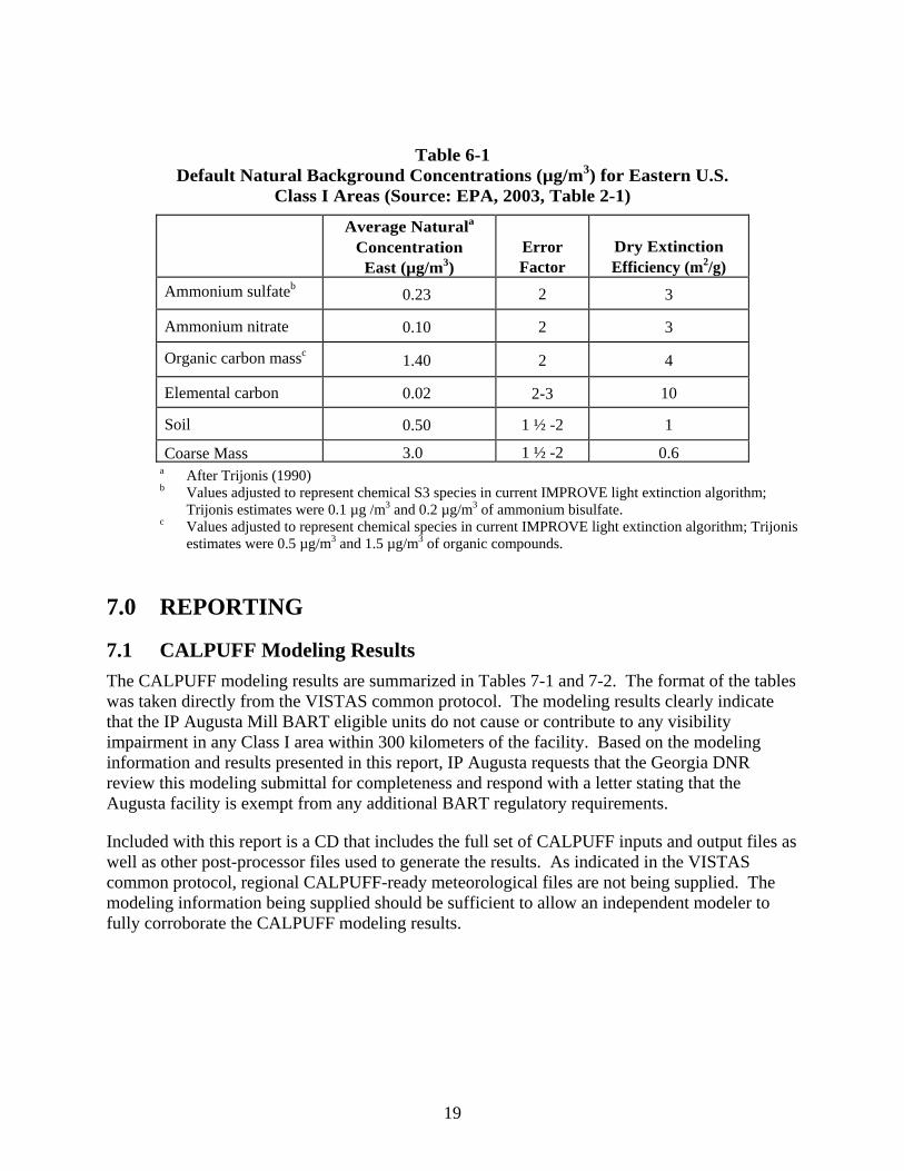
Based on recent regulatory rulings, URS has opted to use the annual average method for calculating natural background conditions. The components for the Eastern U.S. are provided in Table 6-1 and were input to the CALPOST model.
Impact Threshold. The EPA BART guidance recommends that the threshold value for defining whether a source “contributes” to visibility impairment is 0.5-dv change from natural conditions.
When 98th percentile modeling is conducted the highest modeled delta deciview value for each modeling day is determined by using CALPOST. The higher, of the 8th highest value for each year or the 22nd highest over the three year period value is compared to the 0.5-dv contribution threshold value. If the value exceeds the “contribution” threshold of 0.5-dv, the source will be subject to a BART evaluation. If the value is less than the “contribution” threshold 0.5-dv, the source is exempted from the BART requirements.
Since the current regulatory version of CALPOST does not generate 98th percentile results for a three-year period, URS used a simple spreadsheet to determine the 22nd highest values for the three year period by importing the needed information from the CALPOST output file.
19
Table 6-1 Default Natural Background Concentrations (µg/m3) for Eastern U.S.
Class I Areas (Source: EPA, 2003, Table 2-1)
Average Naturala
Concentration East (µg/m3)
Error Factor
Dry Extinction Efficiency (m2/g)
Ammonium sulfateb 0.23 2 3
Ammonium nitrate 0.10 2 3
Organic carbon massc 1.40 2 4
Elemental carbon 0.02 2-3 10
Soil 0.50 1 ½ -2 1
Coarse Mass 3.0 1 ½ -2 0.6 a After Trijonis (1990) b Values adjusted to represent chemical S3 species in current IMPROVE light extinction algorithm;
Trijonis estimates were 0.1 µg /m3 and 0.2 µg/m3 of ammonium bisulfate. c Values adjusted to represent chemical species in current IMPROVE light extinction algorithm; Trijonis
estimates were 0.5 µg/m3 and 1.5 µg/m3 of organic compounds. 7.0 REPORTING
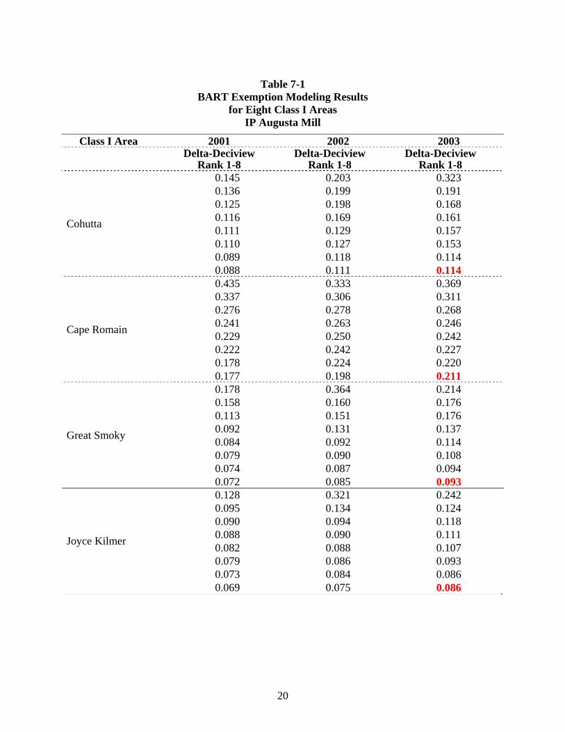
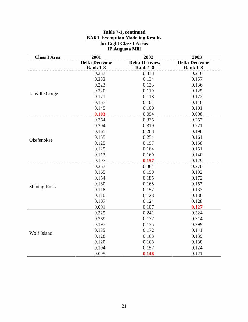
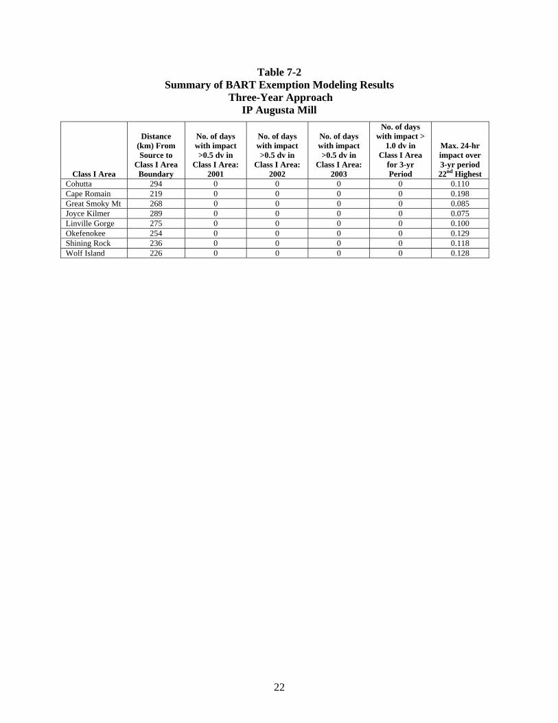
7.1 CALPUFF Modeling Results The CALPUFF modeling results are summarized in Tables 7-1 and 7-2. The format of the tables was taken directly from the VISTAS common protocol. The modeling results clearly indicate that the IP Augusta Mill BART eligible units do not cause or contribute to any visibility impairment in any Class I area within 300 kilometers of the facility. Based on the modeling information and results presented in this report, IP Augusta requests that the Georgia DNR review this modeling submittal for completeness and respond with a letter stating that the Augusta facility is exempt from any additional BART regulatory requirements.
Included with this report is a CD that includes the full set of CALPUFF inputs and output files as well as other post-processor files used to generate the results. As indicated in the VISTAS common protocol, regional CALPUFF-ready meteorological files are not being supplied. The modeling information being supplied should be sufficient to allow an independent modeler to fully corroborate the CALPUFF modeling results.
20
Table 7-1 BART Exemption Modeling Results
for Eight Class I Areas IP Augusta Mill
Class I Area 2001 2002 2003 Delta-Deciview
Rank 1-8 Delta-Deciview
Rank 1-8 Delta-Deciview
Rank 1-8 0.145 0.203 0.323 0.136 0.199 0.191 0.125 0.198 0.168 0.116 0.169 0.161 0.111 0.129 0.157 0.110 0.127 0.153 0.089 0.118 0.114
Cohutta
0.088 0.111 0.114 0.435 0.333 0.369 0.337 0.306 0.311 0.276 0.278 0.268 0.241 0.263 0.246 0.229 0.250 0.242 0.222 0.242 0.227 0.178 0.224 0.220
Cape Romain
0.177 0.198 0.211 0.178 0.364 0.214 0.158 0.160 0.176 0.113 0.151 0.176 0.092 0.131 0.137 0.084 0.092 0.114 0.079 0.090 0.108 0.074 0.087 0.094
Great Smoky
0.072 0.085 0.093 0.128 0.321 0.242 0.095 0.134 0.124 0.090 0.094 0.118 0.088 0.090 0.111 0.082 0.088 0.107 0.079 0.086 0.093 0.073 0.084 0.086
Joyce Kilmer
0.069 0.075 0.086
21
Table 7-1, continued BART Exemption Modeling Results
for Eight Class I Areas IP Augusta Mill
Class I Area 2001 2002 2003 Delta-Deciview
Rank 1-8 Delta-Deciview
Rank 1-8 Delta-Deciview
Rank 1-8 0.237 0.338 0.216 0.232 0.134 0.157 0.223 0.123 0.136 0.220 0.119 0.125 0.171 0.118 0.122 0.157 0.101 0.110 0.145 0.100 0.101
Linville Gorge
0.103 0.094 0.098 0.264 0.335 0.257 0.204 0.319 0.221 0.165 0.268 0.198 0.155 0.254 0.161 0.125 0.197 0.158 0.125 0.164 0.151 0.113 0.160 0.140
Okefenokee
0.107 0.157 0.129 0.257 0.384 0.270 0.165 0.190 0.192 0.154 0.185 0.172 0.130 0.168 0.157 0.118 0.152 0.137 0.110 0.128 0.136 0.107 0.124 0.128
Shining Rock
0.091 0.107 0.127 0.325 0.241 0.324 0.269 0.177 0.314 0.197 0.175 0.299 0.135 0.172 0.141 0.128 0.168 0.139 0.120 0.168 0.138 0.104 0.157 0.124
Wolf Island
0.095 0.148 0.121
22
Table 7-2 Summary of BART Exemption Modeling Results
Three-Year Approach IP Augusta Mill
Class I Area
Distance (km) From Source to
Class I Area Boundary
No. of days with impact >0.5 dv in
Class I Area: 2001
No. of days with impact >0.5 dv in
Class I Area: 2002
No. of days with impact >0.5 dv in
Class I Area: 2003
No. of days with impact >
1.0 dv in Class I Area
for 3-yr Period
Max. 24-hr impact over 3-yr period 22nd Highest
Cohutta 294 0 0 0 0 0.110 Cape Romain 219 0 0 0 0 0.198 Great Smoky Mt 268 0 0 0 0 0.085 Joyce Kilmer 289 0 0 0 0 0.075 Linville Gorge 275 0 0 0 0 0.100 Okefenokee 254 0 0 0 0 0.129 Shining Rock 236 0 0 0 0 0.118 Wolf Island 226 0 0 0 0 0.128
23
8.0 REFERENCES VISTAS, 2006. Protocol for the Application of the CALPUFF Model for Analyses of Best Available Retrofit Technology (BART), December 22, 2005, Revision 3 – 7/17/06 CDPHE, 2005. CALMET/CALPUFF BART Protocol for Class I Federal Area Individual Source Attribution Visibility Impairment Modeling Analysis, prepared by the Air Pollution Control Division, Colorado Department of Public Health and Environment, Denver, CO. Earth Tech, Inc., 2002. “Application of CALMET/CALPUFF and MESOPUFF II to Compare Regulatory Design Concentrations for a Typical Long-Range Transport Analysis”, prepared for U.S. EPA, prepared by Earth Tech, Inc, Concord, MA. EPA, 1995. “Interagency Workgroup on Air Quality Modeling (IWAQM): Assessment of Phase 1 Recommendations Regarding the Use of MESOPUFF II”, EPA- 54/R-95-006. Office of Air Quality Planning and Standards, U.S Environmental Protection Agency, Research Triangle Park, NC 27711. EPA, 1998b. “An Analysis of the CALMET/CALPUFF Modeling System in a Screening Mode.” EPA-454/R-98-010. Office of Air Quality Planning and Standards, U.S. Environmental Protection Agency, Research Triangle Park, NC 27711. EPA, 1998c. “A Comparison of CALPUFF with ISC3.” EPA-454/R-98-020. Office of Air Quality Planning and Standards, U.S. Environmental Protection Agency, Research Triangle Park, NC 27711. EPA, 1998d. Phase 2 Summary Report and Recommendations for Modeling Long Range Transport and Impacts. Interagency Workgroup on Air Quality Modeling (IWAQM). EPA454/R-98-019, U.S. Environmental Protection Agency, RTP, NC. EPA. 1998e. “Response to Peer Review Comments of CALMET/CALPUFF Modeling System.” Research Triangle Park, NC. November. EPA. 1999. “Response to Peer Review Comments of the Interagency Workgroup on Air Quality Modeling Phase 2 Summary Report and Recommendations for Modeling Long Range Transport Impacts.” Research Triangle Park, NC. February. EPA. 1999. Regional Haze Regulations; Final Rule. Federal Register, 64, 357 13-35774. EPA, 2003. Guidance for Estimating Natural Visibility Conditions under the Regional Haze Rule. EPA-454/B-03-005. U.S. Environmental Protection Agency, Research Triangle Park, NC. EPA, 2005. Regional Haze Regulations and Guidelines for Best Available Retrofit Technology (BART) Determinations. Federal Register, 70 (128), Wednesday, July 6, 2005. Escoffier-Czaja, C., and J. Scire. 2002: The Effects of Ammonia Limitation on Nitrate Aerosol Formation and Visibility Impacts in Class I Areas. Paper J5.13, 12th AMS/A&WMA Conference on the Applications of Air Pollution Meteorology, Norfolk, VA. May 2002.
24
Escoffier-Czaja, C., and J. Scire. 2005: Comments on the Computation of Nitrate Using the Ammonia Limiting Method in CALPUFF”, Earth Tech, Inc., Concord, MA. Federal Register. 2003. 40 CFR Part 51. “Revisions to the Guidelines on Air Quality Models: Adoption of a Preferred Long Range Transport Model and Other Revisions; Final Rule. Federal Register/Vol. 68, No 72/Tuesday April 15, 2003. FLAG 2000. “Federal Land Managers’ Air Quality Related Values Workgroup (FLAG)”: Phase I Report. USDI – National Park Service, Air Resources Division, Denver, CO. Garrison, M., A. Gray, S.T. Rao, M. Scruggs, 1999. “Peer Review of the Interagency Workgroup On Air Quality Modeling Phase 2 Summary Report and Recommendations For Modeling Long Range Transport Impacts”, report compiled by: John S. Irwin Air Policy Support Branch, Atmospheric Sciences Modeling Division U.S. Environmental Protection Agency, Research Triangle Park, NC 27711. Irwin, J.S., 1998b. “Interagency Workgroup on Air Quality Modeling (IWAQM): Phase 2 Summary Report and Recommendations for Modeling Long Range Transport Impacts.” EPA-454/R-98-019, Office of Air Quality Planning and Standards, Research Triangle Park, NC, 151 pp. (NTIS Accession Number PB 99-121089). Irwin, J.S. and J.P. Notar. 2001. Long-range-transport screening technique using CALPUFF. Proceedings of Guideline on Air Quality Modeling: A New Beginning AW&MA Specialty Conference. April 4-6, 2001, Newport, RI. Grell, G.A., J. Dudhia, and D.R. Stauffer, 1995: A Description of the Fifth Generation Penn State/NCAR MM5, NCAR TN-398-STR, NCAR Technical Note. IWAQM. 1998. Interagency Workgroup on Air Quality Modeling (IWAQM) Phase 2 Summary Report and Recommendations for Modeling Long-Range Transport and Impacts on Regional Visibility. EPA-454/R-98-019. U.S. Environmental Protection Agency, Office of Air Quality Planning and Standards, Research Triangle Part, NC. Tonnesen G.S., R.E. Morris, M. Uhl, K. Briggs, J. Vimont and T. Moore. 2003. “The WRAP Regional Modeling Center – Application and Evaluation of Regional Visibility Models” presented at 96th Annual Conference and Exhibition of the Air and Waste Management Association, San Diego, California. Tombach, I., 2004. “Options for Estimating Natural Background Visibility in the VISTAS Region”, prepared for the VISTAS Technical Analysis Work Group (TAWG), 15 January. Tombach, I., and P. Brewer, 2005. Natural background visibility and regional haze goals in the Southeastern United States. Journal of the Air & Waste Management Association. (in press). Tombach, I., P. Brewer, T. Rogers, and C. Arrington, 2005a. “BART modeling protocol for VISTAS: First Draft”, 22 March.
25
Tombach, I., P. Brewer, T. Rogers, C. Arrington, J. Scire 2005b. “Protocol for the application of the CALPUFF model for analyses of Best Available Retrofit Technology (BART): VISTAS second draft”, 22 August. Scire, J., I. Tombach, et al. 2005. Protocol for the application of the CALPUFF model for analyses of Best Available Retrofit Technology (BART): (VISTAS third draft), Prepared for the Visibility Improvement State and Tribal Association of the Southeast (VISTAS), Prepared by Earth Tech, Inc., VISTAS Technical Analysis Work Group (TAWG), the Florida Department of Environmental Protection, and the West Virginia Department of Environmental Protection. Scire, J.S., D.G. Strimaitis, and R.J. Yamartino, 2000a: A User’s Guide for the CALPUFF Dispersion Model (Version 5). Earth Tech, Inc., Concord, MA. Scire, J.S., F.R. Robe, M.E. Fernau, and R.J. Yamartino, 2000b: A User’s Guide for the CALMET Meteorological Model (Version 5). Earth Tech, Inc., Concord, MA. Scire, J.S., Z-X Wu, D.G. Strimaitis and G.E. Moore, 2001: The Southwest Wyoming Regional CALPUFF Air Quality Modeling Study – Volume I. Prepared for the Wyoming Dept of Environmental Quality. Available from Earth Tech, Inc., 196 Baker Avenue, Concord, MA. McNally, D. E., 2003. “Annual Application of MM5 for Calendar Year 2001.” Prepared for the U.S. EPA, Office of Air Quality Planning and Standards, Prepared by Alpine Geophysics, LLC, Arvada, CO. 178 pp. McNally, D. E., and T. W. Tesche, 2002. “Annual Meteorological Modeling Protocol: Annual Application of the MM5 to the Continental United States”, prepared for the EPA Office of Air Quality Planning and Standards, Research Triangle Park, NC. Ryan, P., D. Lowenthal and N. Kumar, 2004: Light Extinction Reconstruction in IMPROVE. Presented at the A&WMA Specialty Conference on Regional and Global Perspectives in Haze: Causes, Consequences and Controversies, Asheville, NC, 26-29 October 2004. Johnson, M. T., 2003b. Iowa DNR 2002 Annual MM5 Modeling Project. Presented at the August 11th, 2003 CENRAP Workgroup Meeting in Bloomington, Minnesota. Johnson, M. T., 2005. CALPUFF Modeling Protocol in Support of Best Available Retrofit Technology Determinations”, Prepared by the Iowa Department of Natural Resources, Air Quality Bureau, Des Moines, IA. LADCo, 2005. “Single Source Modeling to Support Regional Haze BART: Version 3”, Prepared by the Lake Michigan Air Directors Consortium (LADCO), Des Plaines, IL. Levy, J., J. Spengler, D, Hlinka, D. Sullivan, and D. Moon, 2002. Using CALPUFF to evaluate the impacts of power plant emissions in Illinois: model sensitivity and implications. Atmospheric Environment. 36 (6). 1063-1075.
26
Morris, R., C. Tana, and G. Yarwood, 2003. “Evaluation of the Sulfate and Nitrate Formation Mechanism in the CALPUFF Modeling System”, Proceedings of the A&WMA Specialty Conference --Guideline on Air Quality Models: The Path Forward. Mystic, CT. 22-24 October. Morris, R.E., B. Koo, T.W. Tesche, C. Loomis, G. Stella, G. Tonnesen, and Z. Wang. 2004a. Modeling protocol for the VISTAS Phase II regional haze modeling. (http://pah.cert.ucr.edu/vistas/vistas2/) MPCA, 2005. “Best Available Retrofit Technology (BART) Modeling Protocol to Determine Sources Subject to BART in the State of Minnesota”, prepared by the Minnesota Pollution Control Agency, St. Paul, MN. NDDH, 2005, “Protocol for BART-Related Visibility Impairment Modeling Analyses in North Dakota”, prepared by the North Dakota Department of Health, Division of Air Quality, Bismarck, ND. NPS, 1993. “Interagency Workgroup on Air Quality Modeling (IWAQM) Phase 1 Report: Interim Recommendation for Modeling Long Range Transport And Impacts On Regional Visibility”, EPA-454/R-93-015, U.S. Environmental Protection Agency, Technical Support Division, Research Triangle Park, NC. Scire, J.S. and F.R. Robe, 1997: Fine-Scale Application of the CALMET Meteorological Model to a Complex Terrain Site. Paper 97-A1313. Air & Waste Management Association 90th Annual Meeting & Exhibition, Toronto, Ontario, Canada. 8-13 June 1997. Scire, J.S., F.W. Lurmann, A. Bass and S.R. Hanna, 1983: Development of the MESOPUFF II Dispersion Model. EPA-600/3-84-057, U.S. Environmental Protection Agency, Research Triangle Park, NC.

APPENDIX A – Emission Rates and Supporting Information
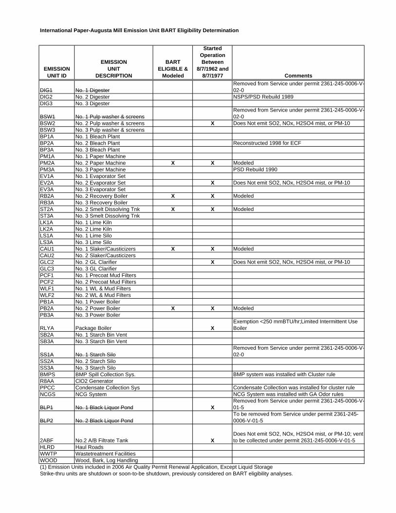
International Paper-Augusta Mill Emission Unit BART Eligibility Determination
EMISSIONUNIT ID
EMISSIONUNIT
DESCRIPTION
BARTELIGIBLE &
Modeled
Started Operation Between
8/7/1962 and 8/7/1977 Comments
DIG1 No. 1 DigesterRemoved from Service under permit 2361-245-0006-V-02-0
DIG2 No. 2 Digester NSPS/PSD Rebuild 1989DIG3 No. 3 Digester
BSW1 No. 1 Pulp washer & screensRemoved from Service under permit 2361-245-0006-V-02-0
BSW2 No. 2 Pulp washer & screens X Does Not emit SO2, NOx, H2SO4 mist, or PM-10BSW3 No. 3 Pulp washer & screensBP1A No. 1 Bleach PlantBP2A No. 2 Bleach Plant Reconstructed 1998 for ECFBP3A No. 3 Bleach PlantPM1A No. 1 Paper MachinePM2A No. 2 Paper Machine X X ModeledPM3A No. 3 Paper Machine PSD Rebuild 1990EV1A No. 1 Evaporator SetEV2A No. 2 Evaporator Set X Does Not emit SO2, NOx, H2SO4 mist, or PM-10EV3A No. 3 Evaporator SetRB2A No. 2 Recovery Boiler X X ModeledRB3A No. 3 Recovery BoilerST2A No. 2 Smelt Dissolving Tnk X X ModeledST3A No. 3 Smelt Dissolving TnkLK1A No. 1 Lime KilnLK2A No. 2 Lime KilnLS1A No. 1 Lime SiloLS3A No. 3 Lime SiloCAU1 No. 1 Slaker/Causticizers X X ModeledCAU2 No. 2 Slaker/CausticizersGLC2 No. 2 GL Clarifier X Does Not emit SO2, NOx, H2SO4 mist, or PM-10GLC3 No. 3 GL ClarifierPCF1 No. 1 Precoat Mud FiltersPCF2 No. 2 Precoat Mud FiltersWLF1 No. 1 WL & Mud FiltersWLF2 No. 2 WL & Mud FiltersPB1A No. 1 Power BoilerPB2A No. 2 Power Boiler X X ModeledPB3A No. 3 Power Boiler
RLYA Package Boiler XExemption <250 mmBTU/hr;Limited Intermittent Use Boiler
SB2A No. 1 Starch Bin VentSB3A No. 3 Starch Bin Vent
SS1A No. 1 Starch SiloRemoved from Service under permit 2361-245-0006-V-02-0
SS2A No. 2 Starch SiloSS3A No. 3 Starch SiloBMPS BMP Spill Collection Sys. BMP system was installed with Cluster ruleR8AA ClO2 GeneratorPPCC Condensate Collection Sys Condensate Collection was installed for cluster rule NCGS NCG System NCG System was installed with GA Odor rules
BLP1 No. 1 Black Liquor Pond XRemoved from Service under permit 2361-245-0006-V-01-5
BLP2 No. 2 Black Liquor PondTo be removed from Service under permit 2361-245-0006-V-01-5
2ABF No.2 A/B Filtrate Tank XDoes Not emit SO2, NOx, H2SO4 mist, or PM-10; vent to be collected under permit 2631-245-0006-V-01-5
HLRD Haul RoadsWWTP Wastetreatment FacilitiesWOOD Wood, Bark, Log Handling(1) Emission Units included in 2006 Air Quality Permit Renewal Application, Except Liquid Storage Strike-thru units are shutdown or soon-to-be shutdown, previously considered on BART eligibility analyses.
INTERNATIONAL PAPER - AUGUSTA MILLBART ELIGIBLE EMISSION UNITS
POINT SOURCE STACK PARAMETERS
UTMEmission System Coordinates Base Stack Horiz Vert Stack StackSource Source X Y Elevation Height Dimension Dimension Temp Velocity Diameter Flow
ID1 Description Type meters meters meters meters meters meters K m/sec meters ACFMPM2A No. 2 Paper Machine V 411142.09 3688250.00 50.5 19.5 14.8 9.1 -- -- -- --PB2A No. 2 Power Boiler P 411316.00 3688176.25 50.5 60.96 -- -- 518.7 20.6 2.74 257,340RB2A No. 2 Recovery Boiler P 411375.41 3688129.25 50.5 60.96 -- -- 430.93 21.8 2.44 215,698ST2A No. 2 Smelt Dissolving Tnk P 411313.84 3688110.25 50.5 39.40 -- -- 336.7 17.8 1.05 32,854
Note - although the Riley package boiler falls within the operational time frame for BART eligible units, it was not modeled as it is a backup boiler <250 MMBtu/hr (not integral to the process).
URS PROJECT NO. 31825278
P:\Common_Projects\2006\BART Exemption Modeling\REPORTS\IP Augusta\BART Tables June06 no Riley 7/28/2006
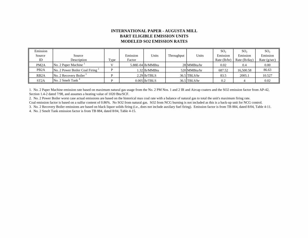
INTERNATIONAL PAPER - AUGUSTA MILLBART ELIGIBLE EMISSION UNITSMODELED SO2 EMISSION RATES
Emission SO2 SO2 SO2
Source Source Emission Units Throughput Units Emission Emission EmissionID Description Type Factor Rate (lb/hr) Rate (lb/day) Rate (g/sec)
PM2A No. 2 Paper Machine 1 V 5.88E-04 lb/MMBtu 28 MMBtu/hr 0.02 0.4 0.00PB2A No. 2 Power Boiler Coal Firing 2 P 1.32 lb/MMBtu 520 MMBtu/hr 687.52 16,500.58 86.63
RB2A No. 2 Recovery Boiler 3 P 2.29 lb/TBLS 36.5 TBLS/hr 83.5 2005.1 10.527ST2A No. 2 Smelt Tank 4 P 0.005 lb/TBLS 36.5 TBLS/hr 0.2 4 0.02
1. No. 2 Paper Machine emission rate based on maximum natural gas usage from the No. 2 PM Nos. 1 and 2 IR and Aircap coaters and the SO2 emission factor from AP-42,Section 1.4-2 dated 7/98, and assumes a heating value of 1020 Btu/SCF.2. No. 2 Power Boiler worst case actual emissions are based on the historical max coal rate with a balance of natural gas to total the unit's maximum firing rate. Coal emission factor is based on a sulfur content of 0.86%. No SO2 from natural gas. SO2 from NCG burning is not included as this is a back-up unit for NCG control.3. No. 2 Recovery Boiler emissions are based on black liquor solids firing (i.e., does not include auxilary fuel firing). Emission factor is from TB 884, dated 8/04, Table 4-11.4. No. 2 Smelt Tank emission factor is from TB 884, dated 8/04, Table 4-15.
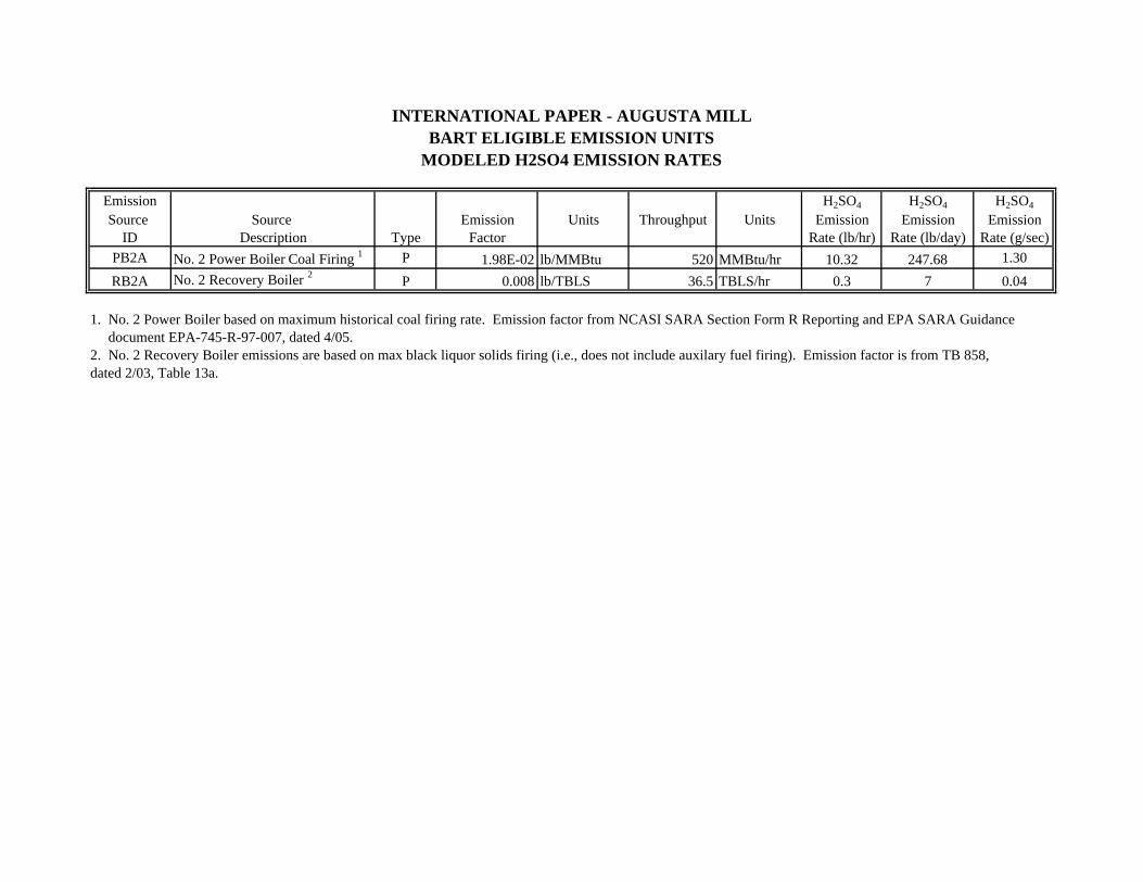
INTERNATIONAL PAPER - AUGUSTA MILLBART ELIGIBLE EMISSION UNITS
MODELED H2SO4 EMISSION RATES
Emission H2SO4 H2SO4 H2SO4
Source Source Emission Units Throughput Units Emission Emission EmissionID Description Type Factor Rate (lb/hr) Rate (lb/day) Rate (g/sec)
PB2A No. 2 Power Boiler Coal Firing 1 P 1.98E-02 lb/MMBtu 520 MMBtu/hr 10.32 247.68 1.30RB2A No. 2 Recovery Boiler 2 P 0.008 lb/TBLS 36.5 TBLS/hr 0.3 7 0.04
1. No. 2 Power Boiler based on maximum historical coal firing rate. Emission factor from NCASI SARA Section Form R Reporting and EPA SARA Guidance document EPA-745-R-97-007, dated 4/05.2. No. 2 Recovery Boiler emissions are based on max black liquor solids firing (i.e., does not include auxilary fuel firing). Emission factor is from TB 858, dated 2/03, Table 13a.
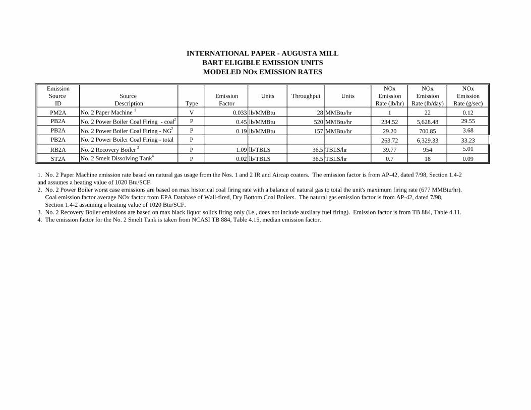
INTERNATIONAL PAPER - AUGUSTA MILLBART ELIGIBLE EMISSION UNITSMODELED NOx EMISSION RATES
Emission NOx NOx NOxSource Source Emission Units Throughput Units Emission Emission Emission
ID Description Type Factor Rate (lb/hr) Rate (lb/day) Rate (g/sec)PM2A No. 2 Paper Machine 1 V 0.033 lb/MMBtu 28 MMBtu/hr 1 22 0.12PB2A No. 2 Power Boiler Coal Firing - coal2 P 0.45 lb/MMBtu 520 MMBtu/hr 234.52 5,628.48 29.55PB2A No. 2 Power Boiler Coal Firing - NG2 P 0.19 lb/MMBtu 157 MMBtu/hr 29.20 700.85 3.68PB2A No. 2 Power Boiler Coal Firing - total P 263.72 6,329.33 33.23RB2A No. 2 Recovery Boiler 3 P 1.09 lb/TBLS 36.5 TBLS/hr 39.77 954 5.01ST2A No. 2 Smelt Dissolving Tank4 P 0.02 lb/TBLS 36.5 TBLS/hr 0.7 18 0.09
1. No. 2 Paper Machine emission rate based on natural gas usage from the Nos. 1 and 2 IR and Aircap coaters. The emission factor is from AP-42, dated 7/98, Section 1.4-2and assumes a heating value of 1020 Btu/SCF.2. No. 2 Power Boiler worst case emissions are based on max historical coal firing rate with a balance of natural gas to total the unit's maximum firing rate (677 MMBtu/hr). Coal emission factor average NOx factor from EPA Database of Wall-fired, Dry Bottom Coal Boilers. The natural gas emission factor is from AP-42, dated 7/98, Section 1.4-2 assuming a heating value of 1020 Btu/SCF. 3. No. 2 Recovery Boiler emissions are based on max black liquor solids firing only (i.e., does not include auxilary fuel firing). Emission factor is from TB 884, Table 4.11.4. The emission factor for the No. 2 Smelt Tank is taken from NCASI TB 884, Table 4.15, median emission factor.
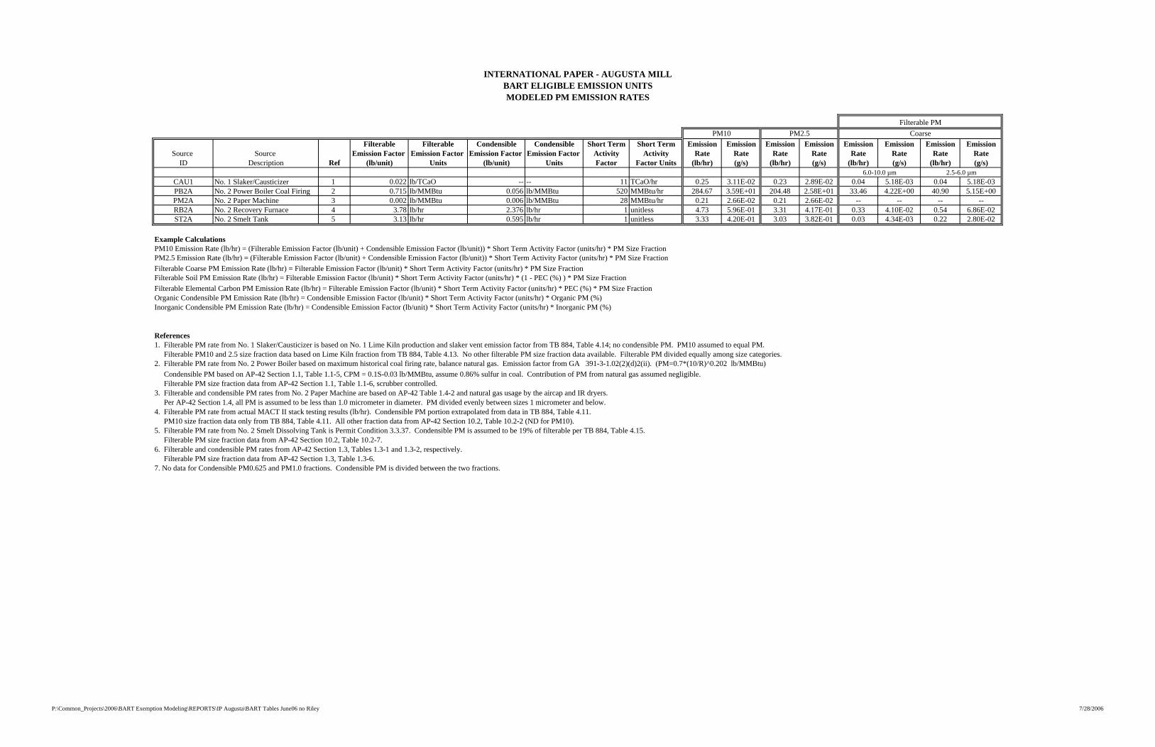
INTERNATIONAL PAPER - AUGUSTA MILLBART ELIGIBLE EMISSION UNITSMODELED PM EMISSION RATES
Filterable PMPM10 PM2.5 Coarse
Filterable Filterable Condensible Condensible Short Term Short Term Emission Emission Emission Emission Emission Emission Emission EmissionSource Source Emission Factor Emission Factor Emission Factor Emission Factor Activity Activity Rate Rate Rate Rate Rate Rate Rate Rate
ID Description Ref (lb/unit) Units (lb/unit) Units Factor Factor Units (lb/hr) (g/s) (lb/hr) (g/s) (lb/hr) (g/s) (lb/hr) (g/s)6.0-10.0 µm 2.5-6.0 µm
CAU1 No. 1 Slaker/Causticizer 1 0.022 lb/TCaO -- -- 11 TCaO/hr 0.25 3.11E-02 0.23 2.89E-02 0.04 5.18E-03 0.04 5.18E-03PB2A No. 2 Power Boiler Coal Firing 2 0.715 lb/MMBtu 0.056 lb/MMBtu 520 MMBtu/hr 284.67 3.59E+01 204.48 2.58E+01 33.46 4.22E+00 40.90 5.15E+00PM2A No. 2 Paper Machine 3 0.002 lb/MMBtu 0.006 lb/MMBtu 28 MMBtu/hr 0.21 2.66E-02 0.21 2.66E-02 -- -- -- --RB2A No. 2 Recovery Furnace 4 3.78 lb/hr 2.376 lb/hr 1 unitless 4.73 5.96E-01 3.31 4.17E-01 0.33 4.10E-02 0.54 6.86E-02ST2A No. 2 Smelt Tank 5 3.13 lb/hr 0.595 lb/hr 1 unitless 3.33 4.20E-01 3.03 3.82E-01 0.03 4.34E-03 0.22 2.80E-02
Example CalculationsPM10 Emission Rate (lb/hr) = (Filterable Emission Factor (lb/unit) + Condensible Emission Factor (lb/unit)) * Short Term Activity Factor (units/hr) * PM Size FractionPM2.5 Emission Rate (lb/hr) = (Filterable Emission Factor (lb/unit) + Condensible Emission Factor (lb/unit)) * Short Term Activity Factor (units/hr) * PM Size FractionFilterable Coarse PM Emission Rate (lb/hr) = Filterable Emission Factor (lb/unit) * Short Term Activity Factor (units/hr) * PM Size FractionFilterable Soil PM Emission Rate (lb/hr) = Filterable Emission Factor (lb/unit) * Short Term Activity Factor (units/hr) * (1 - PEC (%) ) * PM Size FractionFilterable Elemental Carbon PM Emission Rate (lb/hr) = Filterable Emission Factor (lb/unit) * Short Term Activity Factor (units/hr) * PEC (%) * PM Size FractionOrganic Condensible PM Emission Rate (lb/hr) = Condensible Emission Factor (lb/unit) * Short Term Activity Factor (units/hr) * Organic PM (%)Inorganic Condensible PM Emission Rate (lb/hr) = Condensible Emission Factor (lb/unit) * Short Term Activity Factor (units/hr) * Inorganic PM (%)
References1. Filterable PM rate from No. 1 Slaker/Causticizer is based on No. 1 Lime Kiln production and slaker vent emission factor from TB 884, Table 4.14; no condensible PM. PM10 assumed to equal PM. Filterable PM10 and 2.5 size fraction data based on Lime Kiln fraction from TB 884, Table 4.13. No other filterable PM size fraction data available. Filterable PM divided equally among size categories.2. Filterable PM rate from No. 2 Power Boiler based on maximum historical coal firing rate, balance natural gas. Emission factor from GA 391-3-1.02(2)(d)2(ii). (PM=0.7*(10/R)^0.202 lb/MMBtu) Condensible PM based on AP-42 Section 1.1, Table 1.1-5, CPM = 0.1S-0.03 lb/MMBtu, assume 0.86% sulfur in coal. Contribution of PM from natural gas assumed negligible. Filterable PM size fraction data from AP-42 Section 1.1, Table 1.1-6, scrubber controlled.3. Filterable and condensible PM rates from No. 2 Paper Machine are based on AP-42 Table 1.4-2 and natural gas usage by the aircap and IR dryers. Per AP-42 Section 1.4, all PM is assumed to be less than 1.0 micrometer in diameter. PM divided evenly between sizes 1 micrometer and below.4. Filterable PM rate from actual MACT II stack testing results (lb/hr). Condensible PM portion extrapolated from data in TB 884, Table 4.11. PM10 size fraction data only from TB 884, Table 4.11. All other fraction data from AP-42 Section 10.2, Table 10.2-2 (ND for PM10).5. Filterable PM rate from No. 2 Smelt Dissolving Tank is Permit Condition 3.3.37. Condensible PM is assumed to be 19% of filterable per TB 884, Table 4.15. Filterable PM size fraction data from AP-42 Section 10.2, Table 10.2-7.6. Filterable and condensible PM rates from AP-42 Section 1.3, Tables 1.3-1 and 1.3-2, respectively. Filterable PM size fraction data from AP-42 Section 1.3, Table 1.3-6.7. No data for Condensible PM0.625 and PM1.0 fractions. Condensible PM is divided between the two fractions.
P:\Common_Projects\2006\BART Exemption Modeling\REPORTS\IP Augusta\BART Tables June06 no Riley 7/28/2006
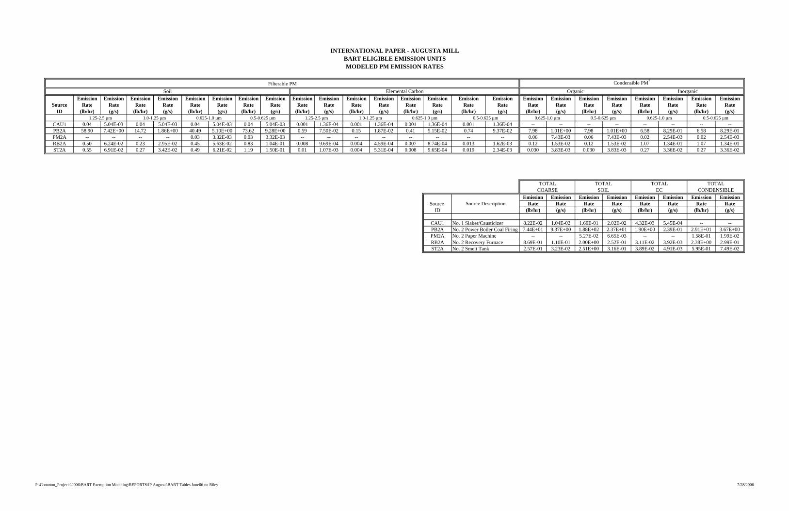
INTERNATIONAL PAPER - AUGUSTA MILLBART ELIGIBLE EMISSION UNITSMODELED PM EMISSION RATES
Filterable PM Condensible PM7
Soil Elemental Carbon Organic InorganicEmission Emission Emission Emission Emission Emission Emission Emission Emission Emission Emission Emission Emission Emission Emission Emission Emission Emission Emission Emission Emission Emission Emission Emission
Source Rate Rate Rate Rate Rate Rate Rate Rate Rate Rate Rate Rate Rate Rate Rate Rate Rate Rate Rate Rate Rate Rate Rate RateID (lb/hr) (g/s) (lb/hr) (g/s) (lb/hr) (g/s) (lb/hr) (g/s) (lb/hr) (g/s) (lb/hr) (g/s) (lb/hr) (g/s) (lb/hr) (g/s) (lb/hr) (g/s) (lb/hr) (g/s) (lb/hr) (g/s) (lb/hr) (g/s)
1.25-2.5 µm 1.0-1.25 µm 0.625-1.0 µm 0.5-0.625 µm 1.25-2.5 µm 1.0-1.25 µm 0.625-1.0 µm 0.5-0.625 µm 0.625-1.0 µm 0.5-0.625 µm 0.625-1.0 µm 0.5-0.625 µmCAU1 0.04 5.04E-03 0.04 5.04E-03 0.04 5.04E-03 0.04 5.04E-03 0.001 1.36E-04 0.001 1.36E-04 0.001 1.36E-04 0.001 1.36E-04 -- -- -- -- -- -- -- --PB2A 58.90 7.42E+00 14.72 1.86E+00 40.49 5.10E+00 73.62 9.28E+00 0.59 7.50E-02 0.15 1.87E-02 0.41 5.15E-02 0.74 9.37E-02 7.98 1.01E+00 7.98 1.01E+00 6.58 8.29E-01 6.58 8.29E-01PM2A -- -- -- -- 0.03 3.32E-03 0.03 3.32E-03 -- -- -- -- -- -- -- -- 0.06 7.43E-03 0.06 7.43E-03 0.02 2.54E-03 0.02 2.54E-03RB2A 0.50 6.24E-02 0.23 2.95E-02 0.45 5.63E-02 0.83 1.04E-01 0.008 9.69E-04 0.004 4.59E-04 0.007 8.74E-04 0.013 1.62E-03 0.12 1.53E-02 0.12 1.53E-02 1.07 1.34E-01 1.07 1.34E-01ST2A 0.55 6.91E-02 0.27 3.42E-02 0.49 6.21E-02 1.19 1.50E-01 0.01 1.07E-03 0.004 5.31E-04 0.008 9.65E-04 0.019 2.34E-03 0.030 3.83E-03 0.030 3.83E-03 0.27 3.36E-02 0.27 3.36E-02
TOTAL TOTAL TOTAL TOTALCOARSE SOIL EC CONDENSIBLE
Emission Emission Emission Emission Emission Emission Emission EmissionSource Rate Rate Rate Rate Rate Rate Rate Rate
ID (lb/hr) (g/s) (lb/hr) (g/s) (lb/hr) (g/s) (lb/hr) (g/s)
CAU1 No. 1 Slaker/Causticizer 8.22E-02 1.04E-02 1.60E-01 2.02E-02 4.32E-03 5.45E-04 -- --PB2A No. 2 Power Boiler Coal Firing 7.44E+01 9.37E+00 1.88E+02 2.37E+01 1.90E+00 2.39E-01 2.91E+01 3.67E+00PM2A No. 2 Paper Machine -- -- 5.27E-02 6.65E-03 -- -- 1.58E-01 1.99E-02RB2A No. 2 Recovery Furnace 8.69E-01 1.10E-01 2.00E+00 2.52E-01 3.11E-02 3.92E-03 2.38E+00 2.99E-01ST2A No. 2 Smelt Tank 2.57E-01 3.23E-02 2.51E+00 3.16E-01 3.89E-02 4.91E-03 5.95E-01 7.49E-02
Source Description
P:\Common_Projects\2006\BART Exemption Modeling\REPORTS\IP Augusta\BART Tables June06 no Riley 7/28/2006
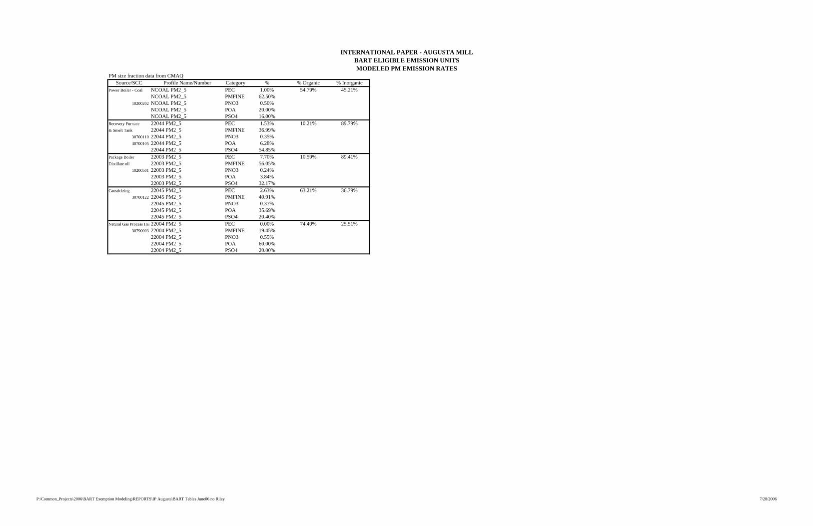
INTERNATIONAL PAPER - AUGUSTA MILLBART ELIGIBLE EMISSION UNITSMODELED PM EMISSION RATES
PM size fraction data from CMAQSource/SCC Profile Name/Number Category % % Organic % Inorganic
Power Boiler - Coal NCOAL PM2_5 PEC 1.00% 54.79% 45.21%NCOAL PM2_5 PMFINE 62.50%
10200202 NCOAL PM2_5 PNO3 0.50%NCOAL PM2_5 POA 20.00%NCOAL PM2_5 PSO4 16.00%
Recovery Furnace 22044 PM2_5 PEC 1.53% 10.21% 89.79%& Smelt Tank 22044 PM2_5 PMFINE 36.99%
30700110 22044 PM2_5 PNO3 0.35%30700105 22044 PM2_5 POA 6.28%
22044 PM2_5 PSO4 54.85%Package Boiler 22003 PM2_5 PEC 7.70% 10.59% 89.41%Distillate oil 22003 PM2_5 PMFINE 56.05%
10200501 22003 PM2_5 PNO3 0.24%22003 PM2_5 POA 3.84%22003 PM2_5 PSO4 32.17%
Causticizing 22045 PM2_5 PEC 2.63% 63.21% 36.79%30700122 22045 PM2_5 PMFINE 40.91%
22045 PM2_5 PNO3 0.37%22045 PM2_5 POA 35.69%22045 PM2_5 PSO4 20.40%
Natural Gas Process Hea22004 PM2_5 PEC 0.00% 74.49% 25.51%30790003 22004 PM2_5 PMFINE 19.45%
22004 PM2_5 PNO3 0.55%22004 PM2_5 POA 60.00%22004 PM2_5 PSO4 20.00%
P:\Common_Projects\2006\BART Exemption Modeling\REPORTS\IP Augusta\BART Tables June06 no Riley 7/28/2006
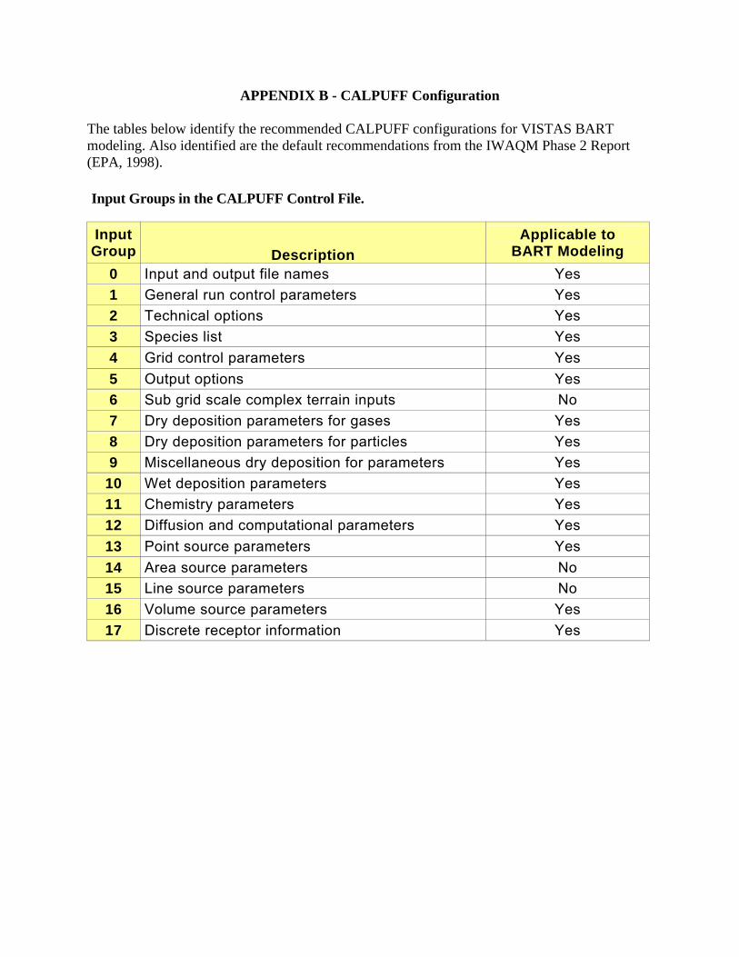
APPENDIX B - CALPUFF Configuration The tables below identify the recommended CALPUFF configurations for VISTAS BART modeling. Also identified are the default recommendations from the IWAQM Phase 2 Report (EPA, 1998).
Input Groups in the CALPUFF Control File.
Input Group Description
Applicable to BART Modeling
0 Input and output file names Yes 1 General run control parameters Yes 2 Technical options Yes 3 Species list Yes 4 Grid control parameters Yes 5 Output options Yes 6 Sub grid scale complex terrain inputs No 7 Dry deposition parameters for gases Yes 8 Dry deposition parameters for particles Yes 9 Miscellaneous dry deposition for parameters Yes
10 Wet deposition parameters Yes 11 Chemistry parameters Yes 12 Diffusion and computational parameters Yes 13 Point source parameters Yes 14 Area source parameters No 15 Line source parameters No 16 Volume source parameters Yes 17 Discrete receptor information Yes
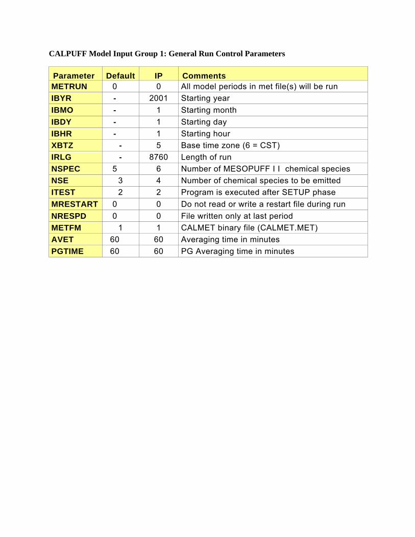
CALPUFF Model Input Group 1: General Run Control Parameters
Parameter Default IP Comments METRUN 0 0 All model periods in met file(s) will be run IBYR - 2001 Starting year IBMO - 1 Starting month IBDY - 1 Starting day IBHR - 1 Starting hour XBTZ - 5 Base time zone (6 = CST) IRLG - 8760 Length of run NSPEC 5 6 Number of MESOPUFF I I chemical species NSE 3 4 Number of chemical species to be emitted ITEST 2 2 Program is executed after SETUP phase MRESTART 0 0 Do not read or write a restart file during run NRESPD 0 0 File written only at last period METFM 1 1 CALMET binary file (CALMET.MET) AVET 60 60 Averaging time in minutes PGTIME 60 60 PG Averaging time in minutes
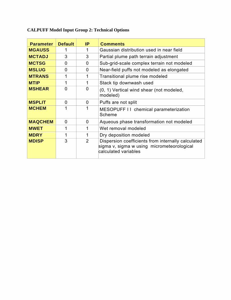
CALPUFF Model Input Group 2: Technical Options
Parameter Default IP Comments MGAUSS 1 1 Gaussian distribution used in near field MCTADJ 3 3 Partial plume path terrain adjustment MCTSG 0 0 Sub-grid-scale complex terrain not modeled MSLUG 0 0 Near-field puffs not modeled as elongated MTRANS 1 1 Transitional plume rise modeled MTIP 1 1 Stack tip downwash used MSHEAR 0 0 (0, 1) Vertical wind shear (not modeled,
modeled) MSPLIT 0 0 Puffs are not split MCHEM 1 1 MESOPUFF I I chemical parameterization
Scheme MAQCHEM 0 0 Aqueous phase transformation not modeled MWET 1 1 Wet removal modeled MDRY 1 1 Dry deposition modeled MDISP 3 2 Dispersion coefficients from internally calculated
sigma v, sigma w using micrometeorological calculated variables
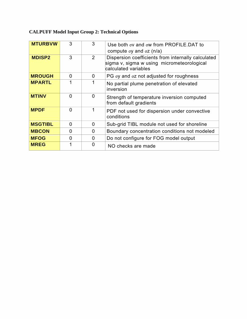
CALPUFF Model Input Group 2: Technical Options
MTURBVW 3 3 Use both σv and σw from PROFILE.DAT to compute σy and σz (n/a)
MDISP2 3 2 Dispersion coefficients from internally calculated sigma v, sigma w using micrometeorological calculated variables
MROUGH 0 0 PG σy and σz not adjusted for roughness MPARTL 1 1 No partial plume penetration of elevated
inversion MTINV 0 0 Strength of temperature inversion computed
from default gradients MPDF 0 1 PDF not used for dispersion under convective
conditions MSGTIBL 0 0 Sub-grid TIBL module not used for shoreline MBCON 0 0 Boundary concentration conditions not modeled MFOG 0 0 Do not configure for FOG model output MREG 1 0 NO checks are made
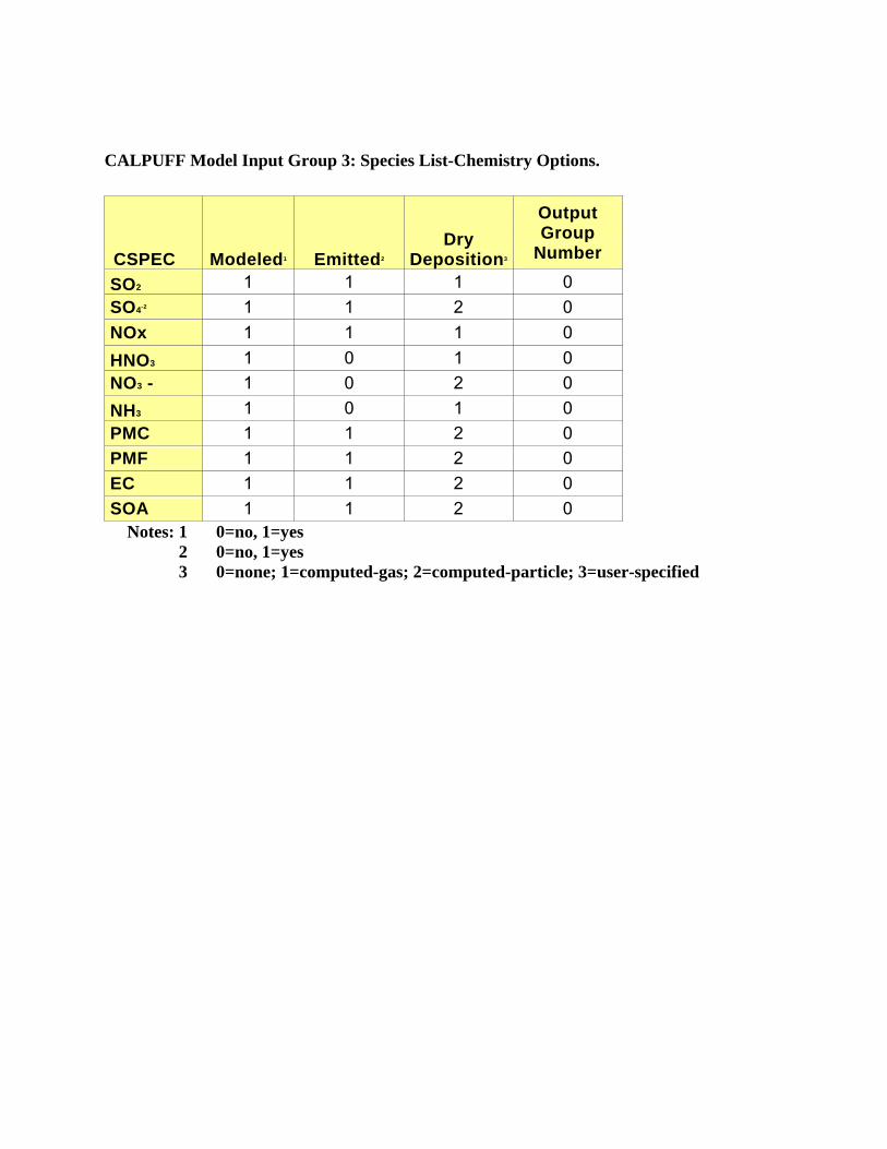
CALPUFF Model Input Group 3: Species List-Chemistry Options.
CSPEC Modeled1 Emitted2 Dry
Deposition3
Output Group
Number
SO2 1 1 1 0 SO4-2 1 1 2 0 NOx 1 1 1 0 HNO3 1 0 1 0 NO3 - 1 0 2 0 NH3 1 0 1 0 PMC 1 1 2 0 PMF 1 1 2 0 EC 1 1 2 0 SOA 1 1 2 0
Notes: 1 0=no, 1=yes 2 0=no, 1=yes 3 0=none; 1=computed-gas; 2=computed-particle; 3=user-specified
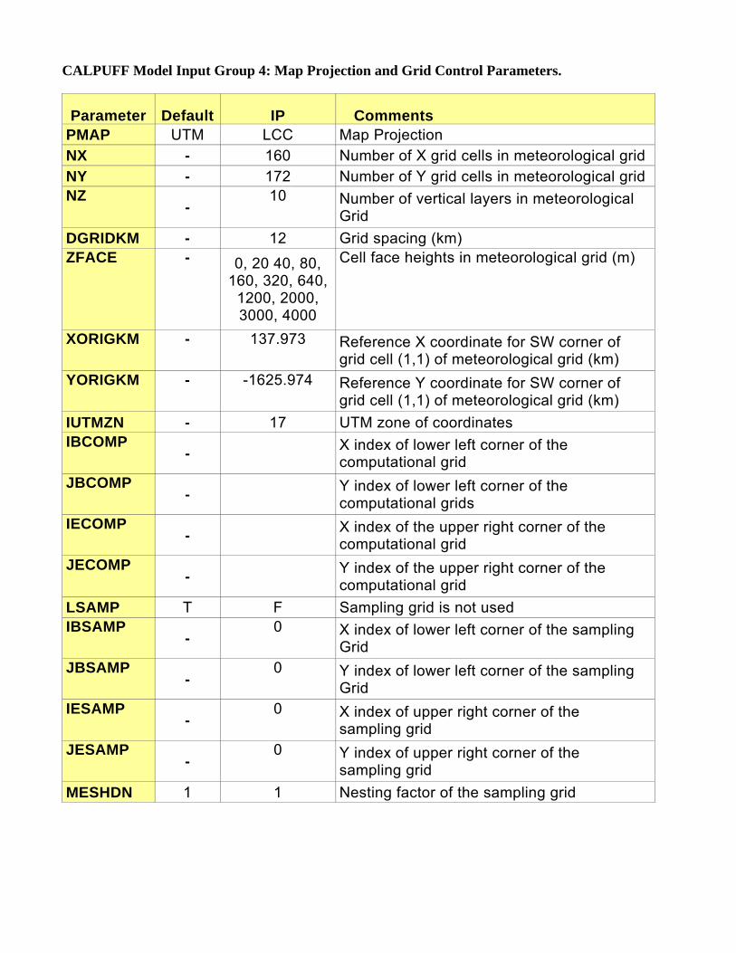
CALPUFF Model Input Group 4: Map Projection and Grid Control Parameters.
Parameter Default IP Comments PMAP UTM LCC Map Projection NX - 160 Number of X grid cells in meteorological grid NY - 172 Number of Y grid cells in meteorological grid NZ
- 10 Number of vertical layers in meteorological
Grid DGRIDKM - 12 Grid spacing (km) ZFACE - 0, 20 40, 80,
160, 320, 640,1200, 2000, 3000, 4000
Cell face heights in meteorological grid (m)
XORIGKM - 137.973 Reference X coordinate for SW corner of grid cell (1,1) of meteorological grid (km)
YORIGKM - -1625.974 Reference Y coordinate for SW corner of grid cell (1,1) of meteorological grid (km)
IUTMZN - 17 UTM zone of coordinates IBCOMP
- X index of lower left corner of the
computational grid JBCOMP
- Y index of lower left corner of the
computational grids IECOMP
- X index of the upper right corner of the
computational grid JECOMP
- Y index of the upper right corner of the
computational grid LSAMP T F Sampling grid is not used IBSAMP
- 0 X index of lower left corner of the sampling
Grid JBSAMP
- 0 Y index of lower left corner of the sampling
Grid IESAMP
- 0 X index of upper right corner of the
sampling grid JESAMP
- 0 Y index of upper right corner of the
sampling grid MESHDN 1 1 Nesting factor of the sampling grid
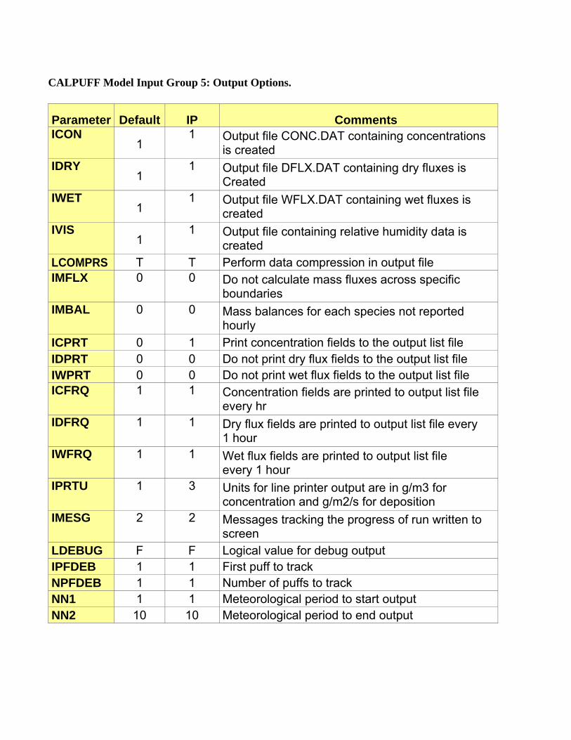
CALPUFF Model Input Group 5: Output Options.
Parameter Default IP Comments ICON
1 1 Output file CONC.DAT containing concentrations
is created IDRY
1 1 Output file DFLX.DAT containing dry fluxes is
Created IWET
1 1 Output file WFLX.DAT containing wet fluxes is
created IVIS
1 1 Output file containing relative humidity data is
created LCOMPRS T T Perform data compression in output file IMFLX 0 0 Do not calculate mass fluxes across specific
boundaries IMBAL 0 0 Mass balances for each species not reported
hourly ICPRT 0 1 Print concentration fields to the output list file IDPRT 0 0 Do not print dry flux fields to the output list file IWPRT 0 0 Do not print wet flux fields to the output list file ICFRQ 1 1 Concentration fields are printed to output list file
every hr IDFRQ 1 1 Dry flux fields are printed to output list file every
1 hour IWFRQ 1 1 Wet flux fields are printed to output list file
every 1 hour IPRTU 1 3 Units for line printer output are in g/m3 for
concentration and g/m2/s for deposition IMESG 2 2 Messages tracking the progress of run written to
screen LDEBUG F F Logical value for debug output IPFDEB 1 1 First puff to track NPFDEB 1 1 Number of puffs to track NN1 1 1 Meteorological period to start output NN2 10 10 Meteorological period to end output
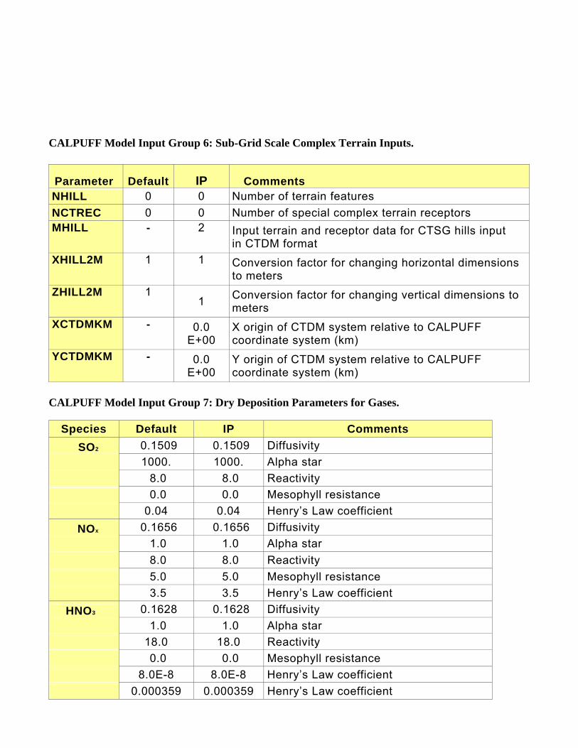
CALPUFF Model Input Group 6: Sub-Grid Scale Complex Terrain Inputs.
Parameter Default IP Comments NHILL 0 0 Number of terrain features NCTREC 0 0 Number of special complex terrain receptors MHILL - 2 Input terrain and receptor data for CTSG hills input
in CTDM format XHILL2M 1 1 Conversion factor for changing horizontal dimensions
to meters ZHILL2M 1
1 Conversion factor for changing vertical dimensions to meters
XCTDMKM - 0.0 E+00
X origin of CTDM system relative to CALPUFF coordinate system (km)
YCTDMKM - 0.0 E+00
Y origin of CTDM system relative to CALPUFF coordinate system (km)
CALPUFF Model Input Group 7: Dry Deposition Parameters for Gases.
Species Default IP Comments SO2 0.1509 0.1509 Diffusivity
1000. 1000. Alpha star 8.0 8.0 Reactivity 0.0 0.0 Mesophyll resistance 0.04 0.04 Henry’s Law coefficient
NOx 0.1656 0.1656 Diffusivity 1.0 1.0 Alpha star 8.0 8.0 Reactivity 5.0 5.0 Mesophyll resistance 3.5 3.5 Henry’s Law coefficient
HNO3 0.1628 0.1628 Diffusivity 1.0 1.0 Alpha star 18.0 18.0 Reactivity 0.0 0.0 Mesophyll resistance 8.0E-8 8.0E-8 Henry’s Law coefficient 0.000359 0.000359 Henry’s Law coefficient
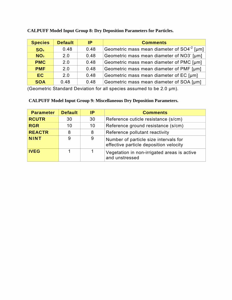
CALPUFF Model Input Group 8: Dry Deposition Parameters for Particles.
Species Default IP Comments SO4 0.48 0.48 Geometric mass mean diameter of SO4-2 [µm]NO3 2.0 0.48 Geometric mass mean diameter of NO3- [µm] PMC 2.0 0.48 Geometric mass mean diameter of PMC [µm] PMF 2.0 0.48 Geometric mass mean diameter of PMF [µm] EC 2.0 0.48 Geometric mass mean diameter of EC [µm]
SOA 0.48 0.48 Geometric mass mean diameter of SOA [µm] (Geometric Standard Deviation for all species assumed to be 2.0 µm).
CALPUFF Model Input Group 9: Miscellaneous Dry Deposition Parameters.
Parameter Default IP Comments RCUTR 30 30 Reference cuticle resistance (s/cm) RGR 10 10 Reference ground resistance (s/cm) REACTR 8 8 Reference pollutant reactivity N I N T 9 9 Number of particle size intervals for
effective particle deposition velocity IVEG 1 1 Vegetation in non-irrigated areas is active
and unstressed
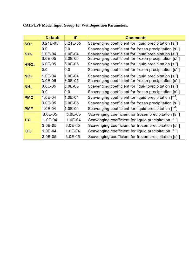
CALPUFF Model Input Group 10: Wet Deposition Parameters.
Default IP Comments SO2 3.21E-05 3.21E-05 Scavenging coefficient for liquid precipitation [s-1]
0.0 0.0 Scavenging coefficient for frozen precipitation [s-1] SO 4 1.0E-04 1.0E-04 Scavenging coefficient for liquid precipitation [s-1] 3.0E-05 3.0E-05 Scavenging coefficient for frozen precipitation [s-1] HNO3 6.0E-05 6.0E-05 Scavenging coefficient for liquid precipitation [s-1]
0.0 0.0 Scavenging coefficient for frozen precipitation [s-1]
NO3 1.0E-04 1.0E-04 Scavenging coefficient for liquid precipitation [s-1] 3.0E-05 3.0E-05 Scavenging coefficient for frozen precipitation [s-1] NH3 8.0E-05 8.0E-05 Scavenging coefficient for liquid precipitation [s-1] 0.0 0.0 Scavenging coefficient for frozen precipitation [s-1] PMC 1.0E-04 1.0E-04 Scavenging coefficient for liquid precipitation [s-1]
3.0E-05 3.0E-05 Scavenging coefficient for frozen precipitation [s-1] PMF 1.0E-04 1.0E-04 Scavenging coefficient for liquid precipitation [s-1]
3.0E-05 3.0E-05 Scavenging coefficient for frozen precipitation [s-1] EC 1.0E-04 1.0E-04 Scavenging coefficient for liquid precipitation [s-1]
3.0E-05 3.0E-05 Scavenging coefficient for frozen precipitation [s-1] OC 1.0E-04 1.0E-04 Scavenging coefficient for liquid precipitation [s-1]
3.0E-05 3.0E-05 Scavenging coefficient for frozen precipitation [s-1]
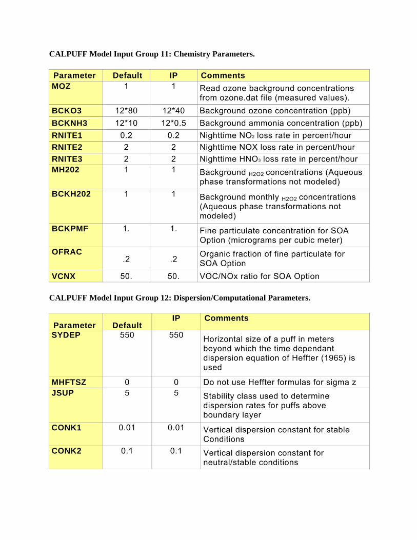
CALPUFF Model Input Group 11: Chemistry Parameters.
Parameter Default IP Comments MOZ 1 1 Read ozone background concentrations
from ozone.dat file (measured values). BCKO3 12*80 12*40 Background ozone concentration (ppb) BCKNH3 12*10 12*0.5 Background ammonia concentration (ppb) RNITE1 0.2 0.2 Nighttime NO2 loss rate in percent/hour RNITE2 2 2 Nighttime NOX loss rate in percent/hour RNITE3 2 2 Nighttime HNO3 loss rate in percent/hour MH202 1 1 Background H2O2 concentrations (Aqueous
phase transformations not modeled) BCKH202 1 1 Background monthly H2O2 concentrations
(Aqueous phase transformations not modeled)
BCKPMF 1. 1. Fine particulate concentration for SOA Option (micrograms per cubic meter)
OFRAC .2 .2 Organic fraction of fine particulate for
SOA Option VCNX 50. 50. VOC/NOx ratio for SOA Option
CALPUFF Model Input Group 12: Dispersion/Computational Parameters.
Parameter Default IP Comments
SYDEP 550 550 Horizontal size of a puff in meters beyond which the time dependant dispersion equation of Heffter (1965) is used
MHFTSZ 0 0 Do not use Heffter formulas for sigma z JSUP 5 5 Stability class used to determine
dispersion rates for puffs above boundary layer
CONK1 0.01 0.01 Vertical dispersion constant for stable Conditions
CONK2 0.1 0.1 Vertical dispersion constant for neutral/stable conditions
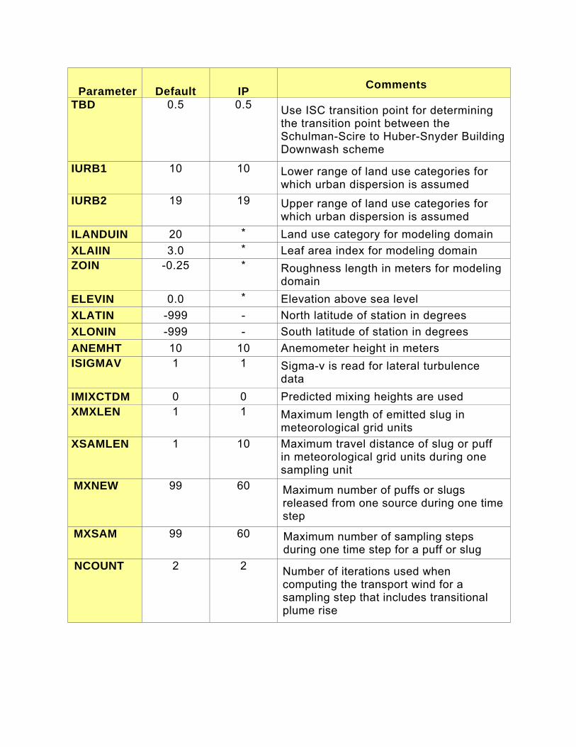
Parameter Default IP Comments
TBD 0.5 0.5 Use ISC transition point for determining the transition point between the Schulman-Scire to Huber-Snyder BuildingDownwash scheme
IURB1 10 10 Lower range of land use categories for which urban dispersion is assumed
IURB2 19 19 Upper range of land use categories for which urban dispersion is assumed
ILANDUIN 20 * Land use category for modeling domain XLAIIN 3.0 * Leaf area index for modeling domain ZOIN -0.25 * Roughness length in meters for modeling
domain ELEVIN 0.0 * Elevation above sea level XLATIN -999 - North latitude of station in degrees XLONIN -999 - South latitude of station in degrees ANEMHT 10 10 Anemometer height in meters ISIGMAV 1 1 Sigma-v is read for lateral turbulence
data IMIXCTDM 0 0 Predicted mixing heights are used XMXLEN 1 1 Maximum length of emitted slug in
meteorological grid units XSAMLEN 1 10 Maximum travel distance of slug or puff
in meteorological grid units during one sampling unit
MXNEW 99 60 Maximum number of puffs or slugs released from one source during one time step
MXSAM 99 60 Maximum number of sampling steps during one time step for a puff or slug
NCOUNT 2 2 Number of iterations used when computing the transport wind for a sampling step that includes transitional plume rise
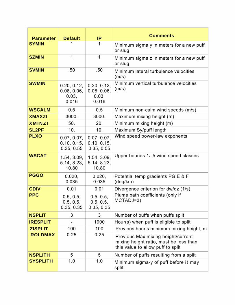
Parameter Default IP Comments
SYMIN 1 1 Minimum sigma y in meters for a new puff or slug
SZMIN 1 1 Minimum sigma z in meters for a new puff or slug
SVMIN .50 .50 Minimum lateral turbulence velocities (m/s)
SWMIN 0.20, 0.12, 0.08, 0.06,
0.03, 0.016
0.20, 0.12,0.08, 0.06,
0.03, 0.016
Minimum vertical turbulence velocities (m/s)
WSCALM 0.5 0.5 Minimum non-calm wind speeds (m/s) XMAXZI 3000. 3000. Maximum mixing height (m) X M I N Z I 50. 20. Minimum mixing height (m) SL2PF 10. 10. Maximum Sy/puff length PLXO 0.07, 0.07,
0.10, 0.15, 0.35, 0.55
0.07, 0.07,0.10, 0.15,0.35, 0.55
Wind speed power-law exponents
WSCAT 1.54, 3.09, 5.14, 8.23,
10.80
1.54, 3.09,5.14, 8.23,
10.80
Upper bounds 1s t 5 wind speed classes
PGGO 0.020, 0.035
0.020, 0.035
Potential temp gradients PG E & F (deg/km)
CDIV 0.01 0.01 Divergence criterion for dw/dz (1/s) PPC 0.5, 0.5,
0.5, 0.5, 0.35, 0.35
0.5, 0.5, 0.5, 0.5,
0.35, 0.35
Plume path coefficients (only if MCTADJ=3)
NSPLIT 3 3 Number of puffs when puffs split IRESPLIT - 1900 Hour(s) when puff is eligible to split ZISPLIT 100 100 Previous hour’s minimum mixing height, mROLDMAX 0.25 0.25 Previous Max mixing height/current
mixing height ratio, must be less than this value to allow puff to split
NSPLITH 5 5 Number of puffs resulting from a split SYSPLITH 1.0 1.0 Minimum sigma-y of puff before i t may
split
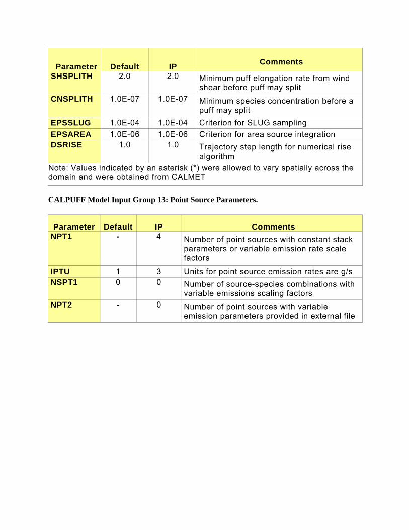
Parameter Default IP Comments
SHSPLITH 2.0 2.0 Minimum puff elongation rate from wind shear before puff may split
CNSPLITH 1.0E-07 1.0E-07 Minimum species concentration before a puff may split
EPSSLUG 1.0E-04 1.0E-04 Criterion for SLUG sampling EPSAREA 1.0E-06 1.0E-06 Criterion for area source integration DSRISE 1.0 1.0 Trajectory step length for numerical rise
algorithm Note: Values indicated by an asterisk (*) were allowed to vary spatially across the domain and were obtained from CALMET CALPUFF Model Input Group 13: Point Source Parameters.
Parameter Default IP Comments NPT1 - 4 Number of point sources with constant stack
parameters or variable emission rate scale factors
IPTU 1 3 Units for point source emission rates are g/s NSPT1 0 0 Number of source-species combinations with
variable emissions scaling factors NPT2 - 0 Number of point sources with variable
emission parameters provided in external file
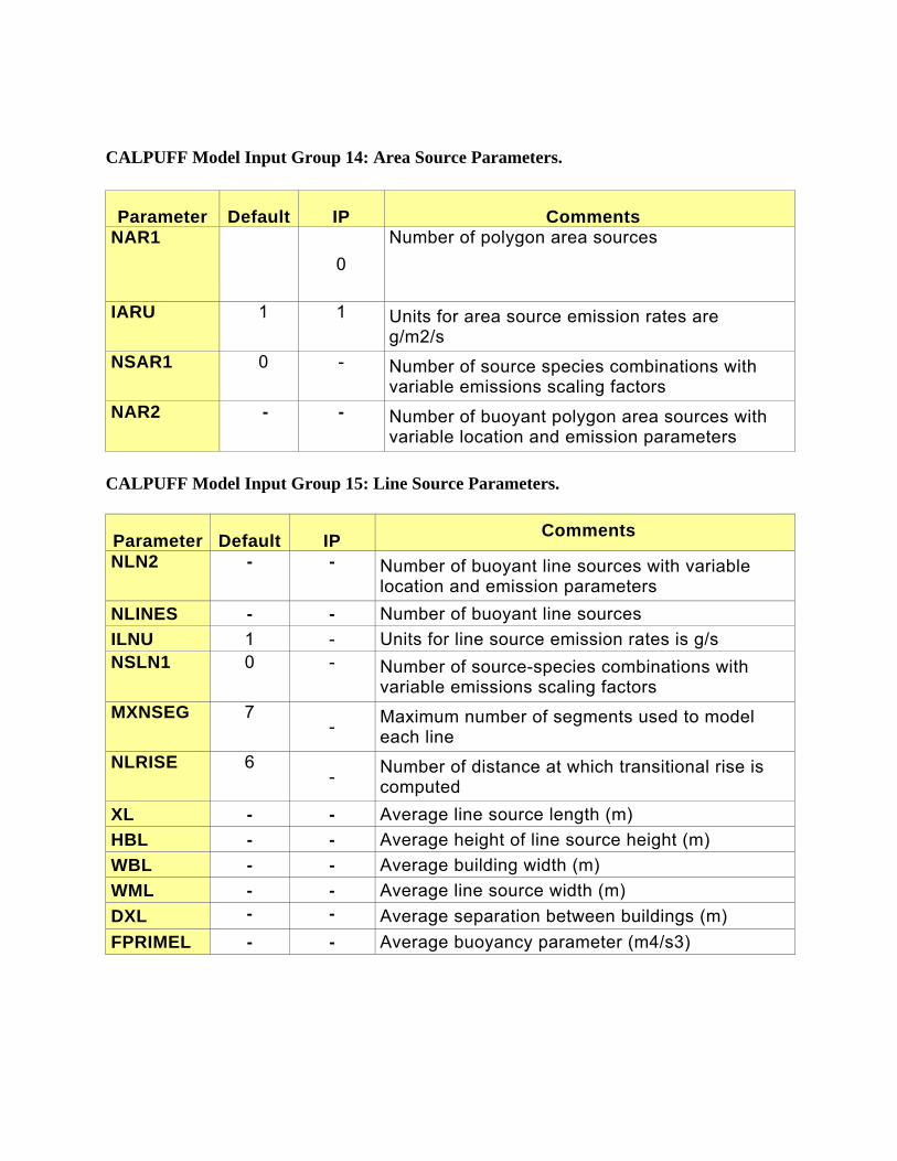
CALPUFF Model Input Group 14: Area Source Parameters.
Parameter Default IP Comments NAR1
0 Number of polygon area sources
IARU 1 1 Units for area source emission rates are g/m2/s
NSAR1 0 - Number of source species combinations with variable emissions scaling factors
NAR2 - - Number of buoyant polygon area sources with variable location and emission parameters
CALPUFF Model Input Group 15: Line Source Parameters.
Parameter Default IP Comments
NLN2 - - Number of buoyant line sources with variable location and emission parameters
NLINES - - Number of buoyant line sources ILNU 1 - Units for line source emission rates is g/s NSLN1 0 - Number of source-species combinations with
variable emissions scaling factors MXNSEG 7
- Maximum number of segments used to model each line
NLRISE 6 - Number of distance at which transitional rise is
computed XL - - Average line source length (m) HBL - - Average height of line source height (m) WBL - - Average building width (m) WML - - Average line source width (m) DXL - - Average separation between buildings (m) FPRIMEL - - Average buoyancy parameter (m4/s3)
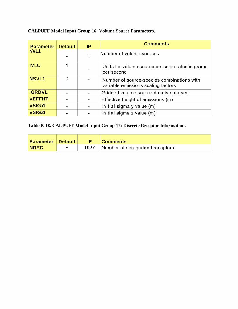
CALPUFF Model Input Group 16: Volume Source Parameters.
Parameter Default IP Comments NVL1
- 1 Number of volume sources
IVLU 1 - Units for volume source emission rates is grams
per second NSVL1 0 - Number of source-species combinations with
variable emissions scaling factors IGRDVL - - Gridded volume source data is not used VEFFHT - - Effective height of emissions (m) VSIGYI - - Init ial sigma y value (m) VSIGZI - - Init ial sigma z value (m)
Table B-18. CALPUFF Model Input Group 17: Discrete Receptor Information.
Parameter Default IP Comments NREC - 1927 Number of non-gridded receptors
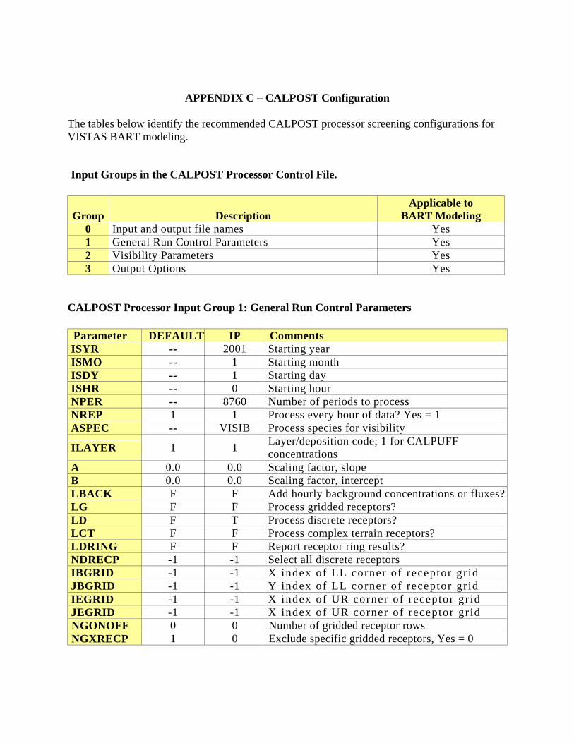
APPENDIX C – CALPOST Configuration The tables below identify the recommended CALPOST processor screening configurations for VISTAS BART modeling.
Input Groups in the CALPOST Processor Control File.
Group Description Applicable to
BART Modeling 0 Input and output file names Yes 1 General Run Control Parameters Yes 2 Visibility Parameters Yes 3 Output Options Yes
CALPOST Processor Input Group 1: General Run Control Parameters
Parameter DEFAULT IP Comments ISYR -- 2001 Starting year ISMO -- 1 Starting month ISDY -- 1 Starting day ISHR -- 0 Starting hour NPER -- 8760 Number of periods to process NREP 1 1 Process every hour of data? Yes = 1 ASPEC -- VISIB Process species for visibility
ILAYER 1 1 Layer/deposition code; 1 for CALPUFF concentrations
A 0.0 0.0 Scaling factor, slope B 0.0 0.0 Scaling factor, intercept LBACK F F Add hourly background concentrations or fluxes?LG F F Process gridded receptors? LD F T Process discrete receptors? LCT F F Process complex terrain receptors? LDRING F F Report receptor ring results? NDRECP -1 -1 Select all discrete receptors IBGRID -1 -1 X index of LL corner of receptor gr id JBGRID -1 -1 Y index of LL corner of receptor gr id IEGRID -1 -1 X index of UR corner of receptor gr id JEGRID -1 -1 X index of UR corner of receptor gr id NGONOFF 0 0 Number of gridded receptor rows NGXRECP 1 0 Exclude specific gridded receptors, Yes = 0
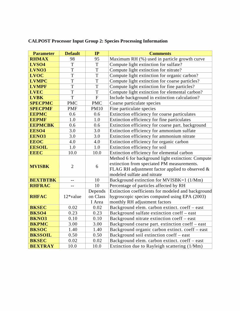
CALPOST Processor Input Group 2: Species Processing Information
Parameter Default IP Comments RHMAX 98 95 Maximum RH (%) used in particle growth curve LVSO4 T T Compute light extinction for sulfate? LVNO3 T T Compute light extinction for nitrate? LVOC T T Compute light extinction for organic carbon? LVMPC T T Compute light extinction for coarse particles? LVMPF T T Compute light extinction for fine particles? LVEC T T Compute light extinction for elemental carbon? LVBK T F Include background in extinction calculation? SPECPMC PMC PMC Coarse particulate species SPECPMF PMF PM10 Fine particulate species EEPMC 0.6 0.6 Extinction efficiency for coarse particulates EEPMF 1.0 1.0 Extinction efficiency for fine particulates EEPMCBK 0.6 0.6 Extinction efficiency for coarse part. background EESO4 3.0 3.0 Extinction efficiency for ammonium sulfate EENO3 3.0 3.0 Extinction efficiency for ammonium nitrate EEOC 4.0 4.0 Extinction efficiency for organic carbon EESOIL 1.0 1.0 Extinction efficiency for soil EEEC 10.0 10.0 Extinction efficiency for elemental carbon
MVISBK 2 6
Method 6 for background light extinction: Compute extinction from speciated PM measurements. FLAG RH adjustment factor applied to observed & modeled sulfate and nitrate
BEXTBTBK -- 10 Background extinction for MVISBK=1 (1/Mm) RHFRAC -- 10 Percentage of particles affected by RH
RHFAC 12*value Depends on Class I Area
Extinction coefficients for modeled and background hygroscopic species computed using EPA (2003) monthly RH adjustment factors
BKSEC 0.02 0.02 Background elem. carbon extinct. coeff – east BKSO4 0.23 0.23 Background sulfate extinction coeff – east BKNO3 0.10 0.10 Background nitrate extinction coeff – east BKPMC 3.00 3.00 Background coarse part. extinction coeff – east BKSOC 1.40 1.40 Background organic carbon extinct. coeff – east BKSSOIL 0.50 0.50 Background soil extinction coeff – east BKSEC 0.02 0.02 Background elem. carbon extinct. coeff – east BEXTRAY 10.0 10.0 Extinction due to Rayleigh scattering (1/Mm)
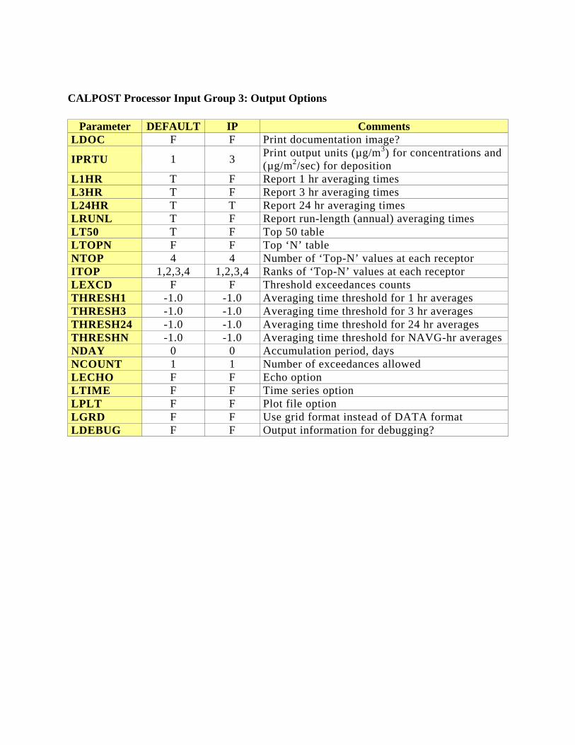
CALPOST Processor Input Group 3: Output Options
Parameter DEFAULT IP Comments LDOC F F Print documentation image?
IPRTU 1 3 Print output units (µg/m3) for concentrations and (µg/m2/sec) for deposition
L1HR T F Report 1 hr averaging times L3HR T F Report 3 hr averaging times L24HR T T Report 24 hr averaging times LRUNL T F Report run-length (annual) averaging times LT50 T F Top 50 table LTOPN F F Top ‘N’ table NTOP 4 4 Number of ‘Top-N’ values at each receptor ITOP 1,2,3,4 1,2,3,4 Ranks of ‘Top-N’ values at each receptor LEXCD F F Threshold exceedances counts THRESH1 -1.0 -1.0 Averaging time threshold for 1 hr averages THRESH3 -1.0 -1.0 Averaging time threshold for 3 hr averages THRESH24 -1.0 -1.0 Averaging time threshold for 24 hr averages THRESHN -1.0 -1.0 Averaging time threshold for NAVG-hr averages NDAY 0 0 Accumulation period, days NCOUNT 1 1 Number of exceedances allowed LECHO F F Echo option LTIME F F Time series option LPLT F F Plot file option LGRD F F Use grid format instead of DATA format LDEBUG F F Output information for debugging?
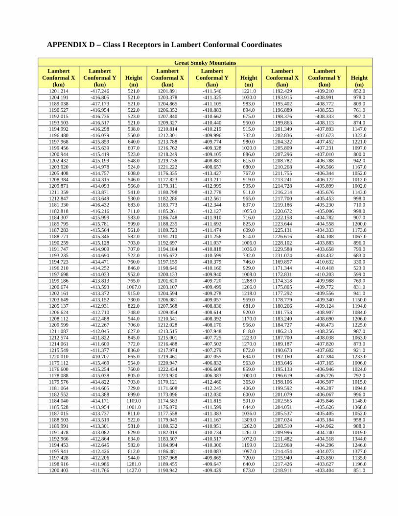
APPENDIX D – Class I Receptors in Lambert Conformal Coordinates
Great Smoky Mountains Lambert
Conformal X (km)
Lambert Conformal Y
(km) Height
(m)
Lambert Conformal X
(km)
Lambert Conformal Y
(km) Height
(m)
Lambert Conformal X
(km)
Lambert Conformal Y
(km) Height
(m) 1201.214 -417.246 521.0 1201.891 -411.546 1221.0 1192.429 -409.210 852.0 1204.191 -416.805 521.0 1203.378 -411.325 1030.0 1193.915 -408.991 978.0 1189.038 -417.173 521.0 1204.865 -411.105 983.0 1195.402 -408.772 809.0 1190.527 -416.954 522.0 1206.352 -410.883 894.0 1196.889 -408.553 761.0 1192.015 -416.736 523.0 1207.840 -410.662 675.0 1198.376 -408.333 987.0 1193.503 -416.517 521.0 1209.327 -410.440 950.0 1199.863 -408.113 874.0 1194.992 -416.298 538.0 1210.814 -410.219 915.0 1201.349 -407.893 1147.0 1196.480 -416.079 550.0 1212.301 -409.996 732.0 1202.836 -407.673 1323.0 1197.968 -415.859 640.0 1213.788 -409.774 980.0 1204.322 -407.452 1221.0 1199.456 -415.639 607.0 1216.762 -409.328 1020.0 1205.809 -407.231 1097.0 1200.944 -415.419 523.0 1218.249 -409.105 886.0 1207.296 -407.010 800.0 1202.432 -415.199 548.0 1219.736 -408.881 615.0 1208.782 -406.788 942.0 1203.920 -414.978 524.0 1221.222 -408.657 680.0 1210.268 -406.566 1167.0 1205.408 -414.757 608.0 1176.335 -413.427 767.0 1211.755 -406.344 1052.0 1208.384 -414.315 546.0 1177.823 -413.211 919.0 1213.241 -406.122 1012.0 1209.871 -414.093 566.0 1179.311 -412.995 905.0 1214.728 -405.899 1002.0 1211.359 -413.871 541.0 1180.798 -412.778 911.0 1216.214 -405.676 1143.0 1212.847 -413.649 530.0 1182.286 -412.561 965.0 1217.700 -405.453 998.0 1181.330 -416.432 683.0 1183.773 -412.344 837.0 1219.186 -405.230 710.0 1182.818 -416.216 711.0 1185.261 -412.127 1055.0 1220.672 -405.006 998.0 1184.307 -415.999 583.0 1186.748 -411.910 716.0 1222.158 -404.782 907.0 1185.795 -415.781 599.0 1188.235 -411.692 825.0 1223.644 -404.558 1200.0 1187.283 -415.564 561.0 1189.723 -411.474 609.0 1225.131 -404.333 1173.0 1188.771 -415.346 582.0 1191.210 -411.256 814.0 1226.616 -404.108 1067.0 1190.259 -415.128 703.0 1192.697 -411.037 1006.0 1228.102 -403.883 896.0 1191.747 -414.909 707.0 1194.184 -410.818 1036.0 1229.588 -403.658 799.0 1193.235 -414.690 522.0 1195.672 -410.599 732.0 1231.074 -403.432 683.0 1194.723 -414.471 760.0 1197.159 -410.379 746.0 1169.857 -410.632 330.0 1196.210 -414.252 846.0 1198.646 -410.160 929.0 1171.344 -410.418 523.0 1197.698 -414.033 952.0 1200.133 -409.940 1008.0 1172.831 -410.203 599.0 1199.186 -413.813 765.0 1201.620 -409.720 1288.0 1174.318 -409.988 769.0 1200.674 -413.593 1067.0 1203.107 -409.499 1266.0 1175.805 -409.772 831.0 1202.161 -413.372 915.0 1204.594 -409.278 1218.0 1177.292 -409.556 941.0 1203.649 -413.152 730.0 1206.081 -409.057 959.0 1178.779 -409.340 1150.0 1205.137 -412.931 822.0 1207.568 -408.836 681.0 1180.266 -409.124 1194.0 1206.624 -412.710 748.0 1209.054 -408.614 920.0 1181.753 -408.907 1084.0 1208.112 -412.488 544.0 1210.541 -408.392 1170.0 1183.240 -408.690 1206.0 1209.599 -412.267 706.0 1212.028 -408.170 956.0 1184.727 -408.473 1225.0 1211.087 -412.045 627.0 1213.515 -407.948 818.0 1186.213 -408.256 987.0 1212.574 -411.822 845.0 1215.001 -407.725 1223.0 1187.700 -408.038 1063.0 1214.061 -411.600 772.0 1216.488 -407.502 1270.0 1189.187 -407.820 873.0 1215.549 -411.377 836.0 1217.974 -407.279 872.0 1190.673 -407.602 921.0 1220.010 -410.707 665.0 1219.461 -407.055 694.0 1192.160 -407.384 1233.0 1175.112 -415.469 554.0 1220.947 -406.832 963.0 1193.646 -407.165 1006.0 1176.600 -415.254 760.0 1222.434 -406.608 859.0 1195.133 -406.946 1024.0 1178.088 -415.038 805.0 1223.920 -406.383 1000.0 1196.619 -406.726 792.0 1179.576 -414.822 703.0 1170.121 -412.460 365.0 1198.106 -406.507 1015.0 1181.064 -414.605 729.0 1171.608 -412.245 406.0 1199.592 -406.287 1094.0 1182.552 -414.388 699.0 1173.096 -412.030 600.0 1201.079 -406.067 996.0 1184.040 -414.171 1109.0 1174.583 -411.815 591.0 1202.565 -405.846 1148.0 1185.528 -413.954 1001.0 1176.070 -411.599 644.0 1204.051 -405.626 1368.0 1187.015 -413.737 811.0 1177.558 -411.383 1036.0 1205.537 -405.405 1052.0 1188.503 -413.519 522.0 1179.045 -411.167 1309.0 1207.024 -405.184 958.0 1189.991 -413.301 581.0 1180.532 -410.951 1262.0 1208.510 -404.962 988.0 1191.478 -413.082 629.0 1182.019 -410.734 1261.0 1209.996 -404.740 1019.0 1192.966 -412.864 634.0 1183.507 -410.517 1072.0 1211.482 -404.518 1344.0 1194.453 -412.645 582.0 1184.994 -410.300 1199.0 1212.968 -404.296 1246.0 1195.941 -412.426 612.0 1186.481 -410.083 1097.0 1214.454 -404.073 1377.0 1197.428 -412.206 944.0 1187.968 -409.865 720.0 1215.940 -403.850 1135.0 1198.916 -411.986 1281.0 1189.455 -409.647 640.0 1217.426 -403.627 1196.0 1200.403 -411.766 1427.0 1190.942 -409.429 873.0 1218.911 -403.404 851.0
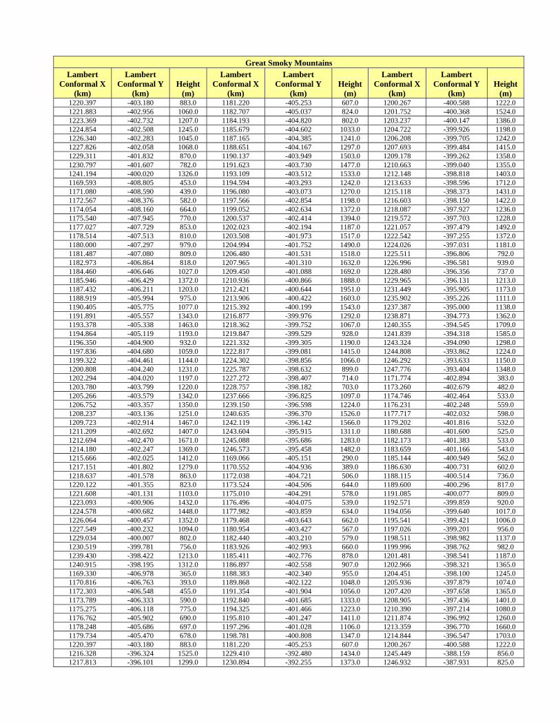
Great Smoky Mountains Lambert
Conformal X (km)
Lambert Conformal Y
(km) Height
(m)
Lambert Conformal X
(km)
Lambert Conformal Y
(km) Height
(m)
Lambert Conformal X
(km)
Lambert Conformal Y
(km) Height
(m) 1220.397 -403.180 883.0 1181.220 -405.253 607.0 1200.267 -400.588 1222.0 1221.883 -402.956 1060.0 1182.707 -405.037 824.0 1201.752 -400.368 1524.0 1223.369 -402.732 1207.0 1184.193 -404.820 802.0 1203.237 -400.147 1386.0 1224.854 -402.508 1245.0 1185.679 -404.602 1033.0 1204.722 -399.926 1198.0 1226.340 -402.283 1045.0 1187.165 -404.385 1241.0 1206.208 -399.705 1242.0 1227.826 -402.058 1068.0 1188.651 -404.167 1297.0 1207.693 -399.484 1415.0 1229.311 -401.832 870.0 1190.137 -403.949 1503.0 1209.178 -399.262 1358.0 1230.797 -401.607 782.0 1191.623 -403.730 1477.0 1210.663 -399.040 1355.0 1241.194 -400.020 1326.0 1193.109 -403.512 1533.0 1212.148 -398.818 1403.0 1169.593 -408.805 453.0 1194.594 -403.293 1242.0 1213.633 -398.596 1712.0 1171.080 -408.590 439.0 1196.080 -403.073 1270.0 1215.118 -398.373 1431.0 1172.567 -408.376 582.0 1197.566 -402.854 1198.0 1216.603 -398.150 1422.0 1174.054 -408.160 664.0 1199.052 -402.634 1372.0 1218.087 -397.927 1236.0 1175.540 -407.945 770.0 1200.537 -402.414 1394.0 1219.572 -397.703 1228.0 1177.027 -407.729 853.0 1202.023 -402.194 1187.0 1221.057 -397.479 1492.0 1178.514 -407.513 810.0 1203.508 -401.973 1517.0 1222.542 -397.255 1372.0 1180.000 -407.297 979.0 1204.994 -401.752 1490.0 1224.026 -397.031 1181.0 1181.487 -407.080 809.0 1206.480 -401.531 1518.0 1225.511 -396.806 792.0 1182.973 -406.864 818.0 1207.965 -401.310 1632.0 1226.996 -396.581 939.0 1184.460 -406.646 1027.0 1209.450 -401.088 1692.0 1228.480 -396.356 737.0 1185.946 -406.429 1372.0 1210.936 -400.866 1888.0 1229.965 -396.131 1213.0 1187.432 -406.211 1203.0 1212.421 -400.644 1951.0 1231.449 -395.905 1173.0 1188.919 -405.994 975.0 1213.906 -400.422 1603.0 1235.902 -395.226 1111.0 1190.405 -405.775 1077.0 1215.392 -400.199 1543.0 1237.387 -395.000 1138.0 1191.891 -405.557 1343.0 1216.877 -399.976 1292.0 1238.871 -394.773 1362.0 1193.378 -405.338 1463.0 1218.362 -399.752 1067.0 1240.355 -394.545 1709.0 1194.864 -405.119 1193.0 1219.847 -399.529 928.0 1241.839 -394.318 1585.0 1196.350 -404.900 932.0 1221.332 -399.305 1190.0 1243.324 -394.090 1298.0 1197.836 -404.680 1059.0 1222.817 -399.081 1415.0 1244.808 -393.862 1224.0 1199.322 -404.461 1144.0 1224.302 -398.856 1066.0 1246.292 -393.633 1150.0 1200.808 -404.240 1231.0 1225.787 -398.632 899.0 1247.776 -393.404 1348.0 1202.294 -404.020 1197.0 1227.272 -398.407 714.0 1171.774 -402.894 383.0 1203.780 -403.799 1220.0 1228.757 -398.182 703.0 1173.260 -402.679 482.0 1205.266 -403.579 1342.0 1237.666 -396.825 1097.0 1174.746 -402.464 533.0 1206.752 -403.357 1350.0 1239.150 -396.598 1224.0 1176.231 -402.248 559.0 1208.237 -403.136 1251.0 1240.635 -396.370 1526.0 1177.717 -402.032 598.0 1209.723 -402.914 1467.0 1242.119 -396.142 1566.0 1179.202 -401.816 532.0 1211.209 -402.692 1407.0 1243.604 -395.915 1311.0 1180.688 -401.600 525.0 1212.694 -402.470 1671.0 1245.088 -395.686 1283.0 1182.173 -401.383 533.0 1214.180 -402.247 1369.0 1246.573 -395.458 1482.0 1183.659 -401.166 543.0 1215.666 -402.025 1412.0 1169.066 -405.151 290.0 1185.144 -400.949 562.0 1217.151 -401.802 1279.0 1170.552 -404.936 389.0 1186.630 -400.731 602.0 1218.637 -401.578 863.0 1172.038 -404.721 506.0 1188.115 -400.514 736.0 1220.122 -401.355 823.0 1173.524 -404.506 644.0 1189.600 -400.296 817.0 1221.608 -401.131 1103.0 1175.010 -404.291 578.0 1191.085 -400.077 809.0 1223.093 -400.906 1432.0 1176.496 -404.075 539.0 1192.571 -399.859 920.0 1224.578 -400.682 1448.0 1177.982 -403.859 634.0 1194.056 -399.640 1017.0 1226.064 -400.457 1352.0 1179.468 -403.643 662.0 1195.541 -399.421 1006.0 1227.549 -400.232 1094.0 1180.954 -403.427 567.0 1197.026 -399.201 956.0 1229.034 -400.007 802.0 1182.440 -403.210 579.0 1198.511 -398.982 1137.0 1230.519 -399.781 756.0 1183.926 -402.993 660.0 1199.996 -398.762 982.0 1239.430 -398.422 1213.0 1185.411 -402.776 878.0 1201.481 -398.541 1187.0 1240.915 -398.195 1312.0 1186.897 -402.558 907.0 1202.966 -398.321 1365.0 1169.330 -406.978 365.0 1188.383 -402.340 955.0 1204.451 -398.100 1245.0 1170.816 -406.763 393.0 1189.868 -402.122 1048.0 1205.936 -397.879 1074.0 1172.303 -406.548 455.0 1191.354 -401.904 1056.0 1207.420 -397.658 1365.0 1173.789 -406.333 590.0 1192.840 -401.685 1333.0 1208.905 -397.436 1401.0 1175.275 -406.118 775.0 1194.325 -401.466 1223.0 1210.390 -397.214 1080.0 1176.762 -405.902 690.0 1195.810 -401.247 1411.0 1211.874 -396.992 1260.0 1178.248 -405.686 697.0 1197.296 -401.028 1106.0 1213.359 -396.770 1660.0 1179.734 -405.470 678.0 1198.781 -400.808 1347.0 1214.844 -396.547 1703.0 1220.397 -403.180 883.0 1181.220 -405.253 607.0 1200.267 -400.588 1222.0 1216.328 -396.324 1525.0 1229.410 -392.480 1434.0 1245.449 -388.159 856.0 1217.813 -396.101 1299.0 1230.894 -392.255 1373.0 1246.932 -387.931 825.0
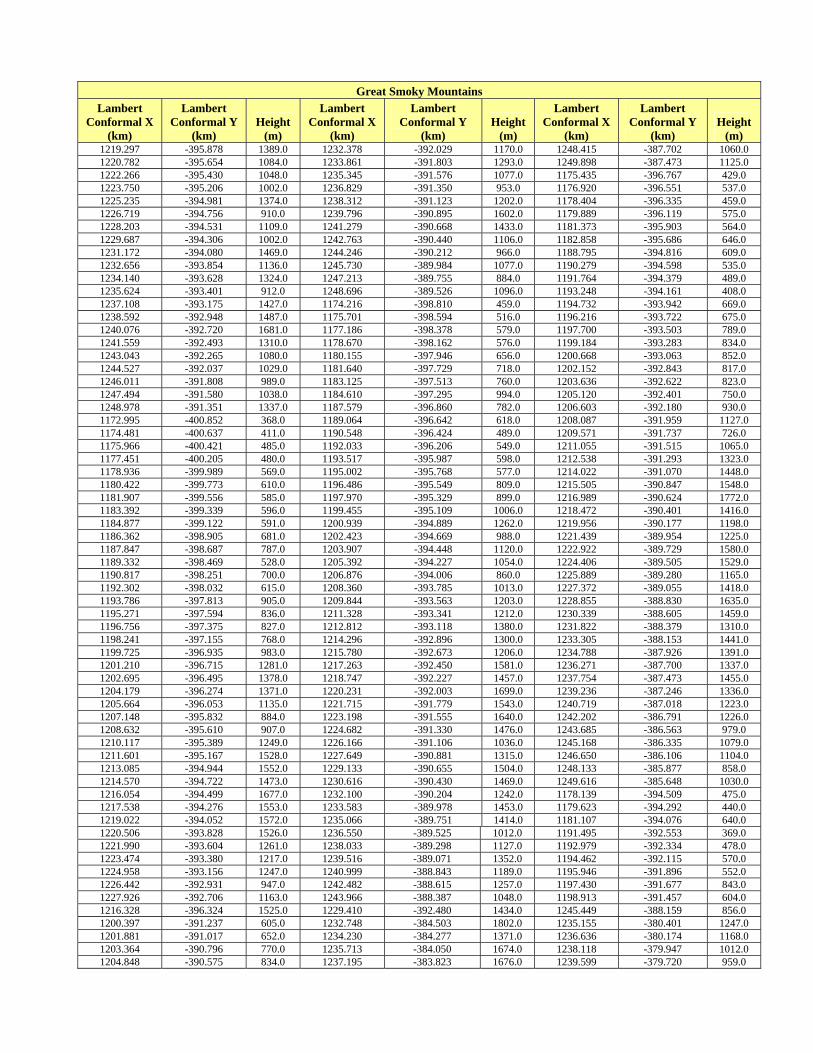
Great Smoky Mountains Lambert
Conformal X (km)
Lambert Conformal Y
(km) Height
(m)
Lambert Conformal X
(km)
Lambert Conformal Y
(km) Height
(m)
Lambert Conformal X
(km)
Lambert Conformal Y
(km) Height
(m) 1219.297 -395.878 1389.0 1232.378 -392.029 1170.0 1248.415 -387.702 1060.0 1220.782 -395.654 1084.0 1233.861 -391.803 1293.0 1249.898 -387.473 1125.0 1222.266 -395.430 1048.0 1235.345 -391.576 1077.0 1175.435 -396.767 429.0 1223.750 -395.206 1002.0 1236.829 -391.350 953.0 1176.920 -396.551 537.0 1225.235 -394.981 1374.0 1238.312 -391.123 1202.0 1178.404 -396.335 459.0 1226.719 -394.756 910.0 1239.796 -390.895 1602.0 1179.889 -396.119 575.0 1228.203 -394.531 1109.0 1241.279 -390.668 1433.0 1181.373 -395.903 564.0 1229.687 -394.306 1002.0 1242.763 -390.440 1106.0 1182.858 -395.686 646.0 1231.172 -394.080 1469.0 1244.246 -390.212 966.0 1188.795 -394.816 609.0 1232.656 -393.854 1136.0 1245.730 -389.984 1077.0 1190.279 -394.598 535.0 1234.140 -393.628 1324.0 1247.213 -389.755 884.0 1191.764 -394.379 489.0 1235.624 -393.401 912.0 1248.696 -389.526 1096.0 1193.248 -394.161 408.0 1237.108 -393.175 1427.0 1174.216 -398.810 459.0 1194.732 -393.942 669.0 1238.592 -392.948 1487.0 1175.701 -398.594 516.0 1196.216 -393.722 675.0 1240.076 -392.720 1681.0 1177.186 -398.378 579.0 1197.700 -393.503 789.0 1241.559 -392.493 1310.0 1178.670 -398.162 576.0 1199.184 -393.283 834.0 1243.043 -392.265 1080.0 1180.155 -397.946 656.0 1200.668 -393.063 852.0 1244.527 -392.037 1029.0 1181.640 -397.729 718.0 1202.152 -392.843 817.0 1246.011 -391.808 989.0 1183.125 -397.513 760.0 1203.636 -392.622 823.0 1247.494 -391.580 1038.0 1184.610 -397.295 994.0 1205.120 -392.401 750.0 1248.978 -391.351 1337.0 1187.579 -396.860 782.0 1206.603 -392.180 930.0 1172.995 -400.852 368.0 1189.064 -396.642 618.0 1208.087 -391.959 1127.0 1174.481 -400.637 411.0 1190.548 -396.424 489.0 1209.571 -391.737 726.0 1175.966 -400.421 485.0 1192.033 -396.206 549.0 1211.055 -391.515 1065.0 1177.451 -400.205 480.0 1193.517 -395.987 598.0 1212.538 -391.293 1323.0 1178.936 -399.989 569.0 1195.002 -395.768 577.0 1214.022 -391.070 1448.0 1180.422 -399.773 610.0 1196.486 -395.549 809.0 1215.505 -390.847 1548.0 1181.907 -399.556 585.0 1197.970 -395.329 899.0 1216.989 -390.624 1772.0 1183.392 -399.339 596.0 1199.455 -395.109 1006.0 1218.472 -390.401 1416.0 1184.877 -399.122 591.0 1200.939 -394.889 1262.0 1219.956 -390.177 1198.0 1186.362 -398.905 681.0 1202.423 -394.669 988.0 1221.439 -389.954 1225.0 1187.847 -398.687 787.0 1203.907 -394.448 1120.0 1222.922 -389.729 1580.0 1189.332 -398.469 528.0 1205.392 -394.227 1054.0 1224.406 -389.505 1529.0 1190.817 -398.251 700.0 1206.876 -394.006 860.0 1225.889 -389.280 1165.0 1192.302 -398.032 615.0 1208.360 -393.785 1013.0 1227.372 -389.055 1418.0 1193.786 -397.813 905.0 1209.844 -393.563 1203.0 1228.855 -388.830 1635.0 1195.271 -397.594 836.0 1211.328 -393.341 1212.0 1230.339 -388.605 1459.0 1196.756 -397.375 827.0 1212.812 -393.118 1380.0 1231.822 -388.379 1310.0 1198.241 -397.155 768.0 1214.296 -392.896 1300.0 1233.305 -388.153 1441.0 1199.725 -396.935 983.0 1215.780 -392.673 1206.0 1234.788 -387.926 1391.0 1201.210 -396.715 1281.0 1217.263 -392.450 1581.0 1236.271 -387.700 1337.0 1202.695 -396.495 1378.0 1218.747 -392.227 1457.0 1237.754 -387.473 1455.0 1204.179 -396.274 1371.0 1220.231 -392.003 1699.0 1239.236 -387.246 1336.0 1205.664 -396.053 1135.0 1221.715 -391.779 1543.0 1240.719 -387.018 1223.0 1207.148 -395.832 884.0 1223.198 -391.555 1640.0 1242.202 -386.791 1226.0 1208.632 -395.610 907.0 1224.682 -391.330 1476.0 1243.685 -386.563 979.0 1210.117 -395.389 1249.0 1226.166 -391.106 1036.0 1245.168 -386.335 1079.0 1211.601 -395.167 1528.0 1227.649 -390.881 1315.0 1246.650 -386.106 1104.0 1213.085 -394.944 1552.0 1229.133 -390.655 1504.0 1248.133 -385.877 858.0 1214.570 -394.722 1473.0 1230.616 -390.430 1469.0 1249.616 -385.648 1030.0 1216.054 -394.499 1677.0 1232.100 -390.204 1242.0 1178.139 -394.509 475.0 1217.538 -394.276 1553.0 1233.583 -389.978 1453.0 1179.623 -394.292 440.0 1219.022 -394.052 1572.0 1235.066 -389.751 1414.0 1181.107 -394.076 640.0 1220.506 -393.828 1526.0 1236.550 -389.525 1012.0 1191.495 -392.553 369.0 1221.990 -393.604 1261.0 1238.033 -389.298 1127.0 1192.979 -392.334 478.0 1223.474 -393.380 1217.0 1239.516 -389.071 1352.0 1194.462 -392.115 570.0 1224.958 -393.156 1247.0 1240.999 -388.843 1189.0 1195.946 -391.896 552.0 1226.442 -392.931 947.0 1242.482 -388.615 1257.0 1197.430 -391.677 843.0 1227.926 -392.706 1163.0 1243.966 -388.387 1048.0 1198.913 -391.457 604.0 1216.328 -396.324 1525.0 1229.410 -392.480 1434.0 1245.449 -388.159 856.0 1200.397 -391.237 605.0 1232.748 -384.503 1802.0 1235.155 -380.401 1247.0 1201.881 -391.017 652.0 1234.230 -384.277 1371.0 1236.636 -380.174 1168.0 1203.364 -390.796 770.0 1235.713 -384.050 1674.0 1238.118 -379.947 1012.0 1204.848 -390.575 834.0 1237.195 -383.823 1676.0 1239.599 -379.720 959.0
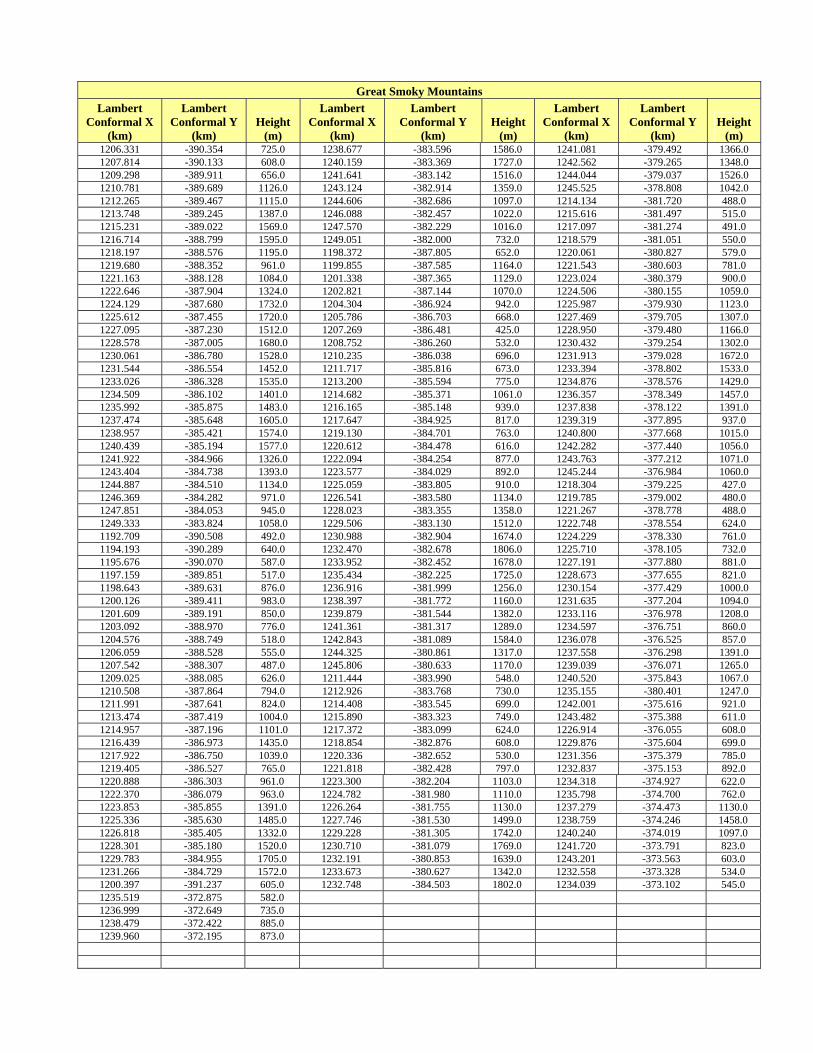
Great Smoky Mountains Lambert
Conformal X (km)
Lambert Conformal Y
(km) Height
(m)
Lambert Conformal X
(km)
Lambert Conformal Y
(km) Height
(m)
Lambert Conformal X
(km)
Lambert Conformal Y
(km) Height
(m) 1206.331 -390.354 725.0 1238.677 -383.596 1586.0 1241.081 -379.492 1366.0 1207.814 -390.133 608.0 1240.159 -383.369 1727.0 1242.562 -379.265 1348.0 1209.298 -389.911 656.0 1241.641 -383.142 1516.0 1244.044 -379.037 1526.0 1210.781 -389.689 1126.0 1243.124 -382.914 1359.0 1245.525 -378.808 1042.0 1212.265 -389.467 1115.0 1244.606 -382.686 1097.0 1214.134 -381.720 488.0 1213.748 -389.245 1387.0 1246.088 -382.457 1022.0 1215.616 -381.497 515.0 1215.231 -389.022 1569.0 1247.570 -382.229 1016.0 1217.097 -381.274 491.0 1216.714 -388.799 1595.0 1249.051 -382.000 732.0 1218.579 -381.051 550.0 1218.197 -388.576 1195.0 1198.372 -387.805 652.0 1220.061 -380.827 579.0 1219.680 -388.352 961.0 1199.855 -387.585 1164.0 1221.543 -380.603 781.0 1221.163 -388.128 1084.0 1201.338 -387.365 1129.0 1223.024 -380.379 900.0 1222.646 -387.904 1324.0 1202.821 -387.144 1070.0 1224.506 -380.155 1059.0 1224.129 -387.680 1732.0 1204.304 -386.924 942.0 1225.987 -379.930 1123.0 1225.612 -387.455 1720.0 1205.786 -386.703 668.0 1227.469 -379.705 1307.0 1227.095 -387.230 1512.0 1207.269 -386.481 425.0 1228.950 -379.480 1166.0 1228.578 -387.005 1680.0 1208.752 -386.260 532.0 1230.432 -379.254 1302.0 1230.061 -386.780 1528.0 1210.235 -386.038 696.0 1231.913 -379.028 1672.0 1231.544 -386.554 1452.0 1211.717 -385.816 673.0 1233.394 -378.802 1533.0 1233.026 -386.328 1535.0 1213.200 -385.594 775.0 1234.876 -378.576 1429.0 1234.509 -386.102 1401.0 1214.682 -385.371 1061.0 1236.357 -378.349 1457.0 1235.992 -385.875 1483.0 1216.165 -385.148 939.0 1237.838 -378.122 1391.0 1237.474 -385.648 1605.0 1217.647 -384.925 817.0 1239.319 -377.895 937.0 1238.957 -385.421 1574.0 1219.130 -384.701 763.0 1240.800 -377.668 1015.0 1240.439 -385.194 1577.0 1220.612 -384.478 616.0 1242.282 -377.440 1056.0 1241.922 -384.966 1326.0 1222.094 -384.254 877.0 1243.763 -377.212 1071.0 1243.404 -384.738 1393.0 1223.577 -384.029 892.0 1245.244 -376.984 1060.0 1244.887 -384.510 1134.0 1225.059 -383.805 910.0 1218.304 -379.225 427.0 1246.369 -384.282 971.0 1226.541 -383.580 1134.0 1219.785 -379.002 480.0 1247.851 -384.053 945.0 1228.023 -383.355 1358.0 1221.267 -378.778 488.0 1249.333 -383.824 1058.0 1229.506 -383.130 1512.0 1222.748 -378.554 624.0 1192.709 -390.508 492.0 1230.988 -382.904 1674.0 1224.229 -378.330 761.0 1194.193 -390.289 640.0 1232.470 -382.678 1806.0 1225.710 -378.105 732.0 1195.676 -390.070 587.0 1233.952 -382.452 1678.0 1227.191 -377.880 881.0 1197.159 -389.851 517.0 1235.434 -382.225 1725.0 1228.673 -377.655 821.0 1198.643 -389.631 876.0 1236.916 -381.999 1256.0 1230.154 -377.429 1000.0 1200.126 -389.411 983.0 1238.397 -381.772 1160.0 1231.635 -377.204 1094.0 1201.609 -389.191 850.0 1239.879 -381.544 1382.0 1233.116 -376.978 1208.0 1203.092 -388.970 776.0 1241.361 -381.317 1289.0 1234.597 -376.751 860.0 1204.576 -388.749 518.0 1242.843 -381.089 1584.0 1236.078 -376.525 857.0 1206.059 -388.528 555.0 1244.325 -380.861 1317.0 1237.558 -376.298 1391.0 1207.542 -388.307 487.0 1245.806 -380.633 1170.0 1239.039 -376.071 1265.0 1209.025 -388.085 626.0 1211.444 -383.990 548.0 1240.520 -375.843 1067.0 1210.508 -387.864 794.0 1212.926 -383.768 730.0 1235.155 -380.401 1247.0 1211.991 -387.641 824.0 1214.408 -383.545 699.0 1242.001 -375.616 921.0 1213.474 -387.419 1004.0 1215.890 -383.323 749.0 1243.482 -375.388 611.0 1214.957 -387.196 1101.0 1217.372 -383.099 624.0 1226.914 -376.055 608.0 1216.439 -386.973 1435.0 1218.854 -382.876 608.0 1229.876 -375.604 699.0 1217.922 -386.750 1039.0 1220.336 -382.652 530.0 1231.356 -375.379 785.0 1219.405 -386.527 765.0 1221.818 -382.428 797.0 1232.837 -375.153 892.0 1220.888 -386.303 961.0 1223.300 -382.204 1103.0 1234.318 -374.927 622.0 1222.370 -386.079 963.0 1224.782 -381.980 1110.0 1235.798 -374.700 762.0 1223.853 -385.855 1391.0 1226.264 -381.755 1130.0 1237.279 -374.473 1130.0 1225.336 -385.630 1485.0 1227.746 -381.530 1499.0 1238.759 -374.246 1458.0 1226.818 -385.405 1332.0 1229.228 -381.305 1742.0 1240.240 -374.019 1097.0 1228.301 -385.180 1520.0 1230.710 -381.079 1769.0 1241.720 -373.791 823.0 1229.783 -384.955 1705.0 1232.191 -380.853 1639.0 1243.201 -373.563 603.0 1231.266 -384.729 1572.0 1233.673 -380.627 1342.0 1232.558 -373.328 534.0 1200.397 -391.237 605.0 1232.748 -384.503 1802.0 1234.039 -373.102 545.0 1235.519 -372.875 582.0 1236.999 -372.649 735.0 1238.479 -372.422 885.0 1239.960 -372.195 873.0

Great Smoky Mountains Lambert
Conformal X (km)
Lambert Conformal Y
(km) Height
(m)
Lambert Conformal X
(km)
Lambert Conformal Y
(km) Height
(m)
Lambert Conformal X
(km)
Lambert Conformal Y
(km) Height
(m)
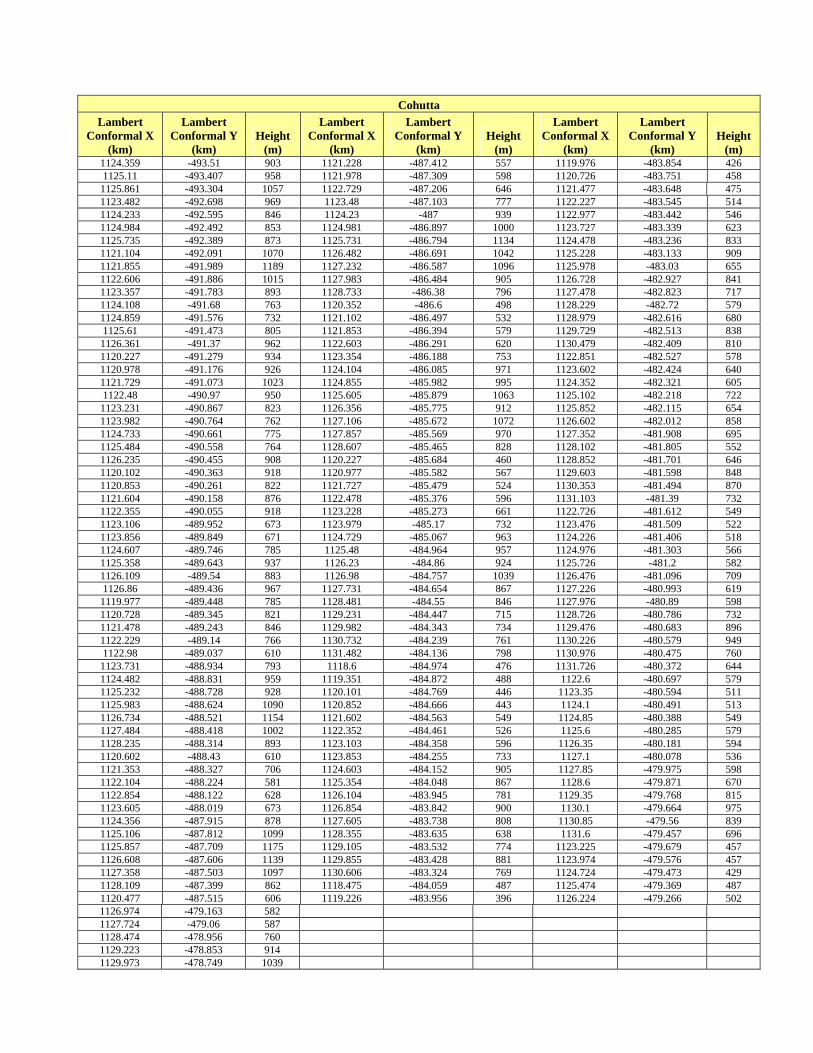
Cohutta
Lambert Conformal X
(km)
Lambert Conformal Y
(km) Height
(m)
Lambert Conformal X
(km)
Lambert Conformal Y
(km) Height
(m)
Lambert Conformal X
(km)
Lambert Conformal Y
(km) Height
(m) 1124.359 -493.51 903 1121.228 -487.412 557 1119.976 -483.854 426 1125.11 -493.407 958 1121.978 -487.309 598 1120.726 -483.751 458 1125.861 -493.304 1057 1122.729 -487.206 646 1121.477 -483.648 475 1123.482 -492.698 969 1123.48 -487.103 777 1122.227 -483.545 514 1124.233 -492.595 846 1124.23 -487 939 1122.977 -483.442 546 1124.984 -492.492 853 1124.981 -486.897 1000 1123.727 -483.339 623 1125.735 -492.389 873 1125.731 -486.794 1134 1124.478 -483.236 833 1121.104 -492.091 1070 1126.482 -486.691 1042 1125.228 -483.133 909 1121.855 -491.989 1189 1127.232 -486.587 1096 1125.978 -483.03 655 1122.606 -491.886 1015 1127.983 -486.484 905 1126.728 -482.927 841 1123.357 -491.783 893 1128.733 -486.38 796 1127.478 -482.823 717 1124.108 -491.68 763 1120.352 -486.6 498 1128.229 -482.72 579 1124.859 -491.576 732 1121.102 -486.497 532 1128.979 -482.616 680 1125.61 -491.473 805 1121.853 -486.394 579 1129.729 -482.513 838 1126.361 -491.37 962 1122.603 -486.291 620 1130.479 -482.409 810 1120.227 -491.279 934 1123.354 -486.188 753 1122.851 -482.527 578 1120.978 -491.176 926 1124.104 -486.085 971 1123.602 -482.424 640 1121.729 -491.073 1023 1124.855 -485.982 995 1124.352 -482.321 605 1122.48 -490.97 950 1125.605 -485.879 1063 1125.102 -482.218 722 1123.231 -490.867 823 1126.356 -485.775 912 1125.852 -482.115 654 1123.982 -490.764 762 1127.106 -485.672 1072 1126.602 -482.012 858 1124.733 -490.661 775 1127.857 -485.569 970 1127.352 -481.908 695 1125.484 -490.558 764 1128.607 -485.465 828 1128.102 -481.805 552 1126.235 -490.455 908 1120.227 -485.684 460 1128.852 -481.701 646 1120.102 -490.363 918 1120.977 -485.582 567 1129.603 -481.598 848 1120.853 -490.261 822 1121.727 -485.479 524 1130.353 -481.494 870 1121.604 -490.158 876 1122.478 -485.376 596 1131.103 -481.39 732 1122.355 -490.055 918 1123.228 -485.273 661 1122.726 -481.612 549 1123.106 -489.952 673 1123.979 -485.17 732 1123.476 -481.509 522 1123.856 -489.849 671 1124.729 -485.067 963 1124.226 -481.406 518 1124.607 -489.746 785 1125.48 -484.964 957 1124.976 -481.303 566 1125.358 -489.643 937 1126.23 -484.86 924 1125.726 -481.2 582 1126.109 -489.54 883 1126.98 -484.757 1039 1126.476 -481.096 709 1126.86 -489.436 967 1127.731 -484.654 867 1127.226 -480.993 619 1119.977 -489.448 785 1128.481 -484.55 846 1127.976 -480.89 598 1120.728 -489.345 821 1129.231 -484.447 715 1128.726 -480.786 732 1121.478 -489.243 846 1129.982 -484.343 734 1129.476 -480.683 896 1122.229 -489.14 766 1130.732 -484.239 761 1130.226 -480.579 949 1122.98 -489.037 610 1131.482 -484.136 798 1130.976 -480.475 760 1123.731 -488.934 793 1118.6 -484.974 476 1131.726 -480.372 644 1124.482 -488.831 959 1119.351 -484.872 488 1122.6 -480.697 579 1125.232 -488.728 928 1120.101 -484.769 446 1123.35 -480.594 511 1125.983 -488.624 1090 1120.852 -484.666 443 1124.1 -480.491 513 1126.734 -488.521 1154 1121.602 -484.563 549 1124.85 -480.388 549 1127.484 -488.418 1002 1122.352 -484.461 526 1125.6 -480.285 579 1128.235 -488.314 893 1123.103 -484.358 596 1126.35 -480.181 594 1120.602 -488.43 610 1123.853 -484.255 733 1127.1 -480.078 536 1121.353 -488.327 706 1124.603 -484.152 905 1127.85 -479.975 598 1122.104 -488.224 581 1125.354 -484.048 867 1128.6 -479.871 670 1122.854 -488.122 628 1126.104 -483.945 781 1129.35 -479.768 815 1123.605 -488.019 673 1126.854 -483.842 900 1130.1 -479.664 975 1124.356 -487.915 878 1127.605 -483.738 808 1130.85 -479.56 839 1125.106 -487.812 1099 1128.355 -483.635 638 1131.6 -479.457 696 1125.857 -487.709 1175 1129.105 -483.532 774 1123.225 -479.679 457 1126.608 -487.606 1139 1129.855 -483.428 881 1123.974 -479.576 457 1127.358 -487.503 1097 1130.606 -483.324 769 1124.724 -479.473 429 1128.109 -487.399 862 1118.475 -484.059 487 1125.474 -479.369 487 1120.477 -487.515 606 1119.226 -483.956 396 1126.224 -479.266 502 1126.974 -479.163 582 1127.724 -479.06 587 1128.474 -478.956 760 1129.223 -478.853 914 1129.973 -478.749 1039
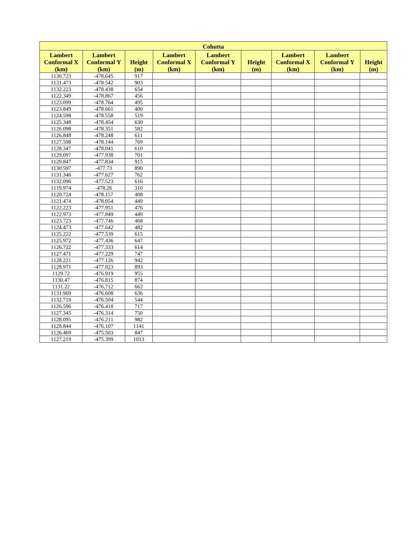
Cohutta Lambert
Conformal X (km)
Lambert Conformal Y
(km) Height
(m)
Lambert Conformal X
(km)
Lambert Conformal Y
(km) Height
(m)
Lambert Conformal X
(km)
Lambert Conformal Y
(km) Height
(m) 1130.723 -478.645 917 1131.473 -478.542 903 1132.223 -478.438 654 1122.349 -478.867 456 1123.099 -478.764 495 1123.849 -478.661 400 1124.598 -478.558 519 1125.348 -478.454 630 1126.098 -478.351 582 1126.848 -478.248 611 1127.598 -478.144 769 1128.347 -478.041 610 1129.097 -477.938 701 1129.847 -477.834 915 1130.597 -477.73 890 1131.346 -477.627 762 1132.096 -477.523 616 1119.974 -478.26 310 1120.724 -478.157 408 1121.474 -478.054 449 1122.223 -477.951 476 1122.973 -477.849 449 1123.723 -477.746 468 1124.473 -477.642 482 1125.222 -477.539 615 1125.972 -477.436 647 1126.722 -477.333 614 1127.471 -477.229 747 1128.221 -477.126 942 1128.971 -477.023 893 1129.72 -476.919 955 1130.47 -476.815 874 1131.22 -476.712 662
1131.969 -476.608 636 1132.719 -476.504 544 1126.596 -476.418 717 1127.345 -476.314 750 1128.095 -476.211 982 1128.844 -476.107 1141 1126.469 -475.503 847 1127.219 -475.399 1013
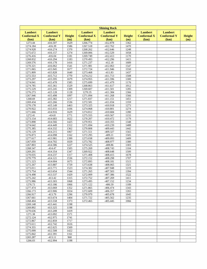
Shining Rock
Lambert Conformal X
(km)
Lambert Conformal Y
(km) Height
(m)
Lambert Conformal X
(km)
Lambert Conformal Y
(km) Height
(m)
Lambert Conformal X
(km)
Lambert Conformal Y
(km) Height
(m) 1273.44 -416.507 1629 1266.774 -412.878 1362 1274.184 -416.39 1586 1267.518 -412.762 1470 1274.928 -416.274 1370 1268.262 -412.646 1248 1275.672 -416.157 1274 1269.006 -412.529 1058 1276.416 -416.04 1181 1269.749 -412.413 1170 1268.832 -416.294 1183 1270.493 -412.296 1415 1269.576 -416.178 1416 1271.237 -412.18 1689 1270.321 -416.062 1541 1271.981 -412.063 1547 1271.065 -415.945 1677 1272.724 -411.946 1550 1271.809 -415.828 1640 1273.468 -411.83 1437 1272.553 -415.712 1770 1274.212 -411.713 1508 1273.297 -415.595 1679 1274.955 -411.596 1300 1274.041 -415.478 1585 1275.699 -411.479 1176 1274.785 -415.361 1529 1268.863 -411.617 1012 1275.529 -415.245 1309 1269.607 -411.501 1285 1276.273 -415.128 1128 1270.35 -411.384 1366 1267.946 -415.498 1097 1271.094 -411.268 1566 1268.69 -415.382 1217 1271.837 -411.151 1451 1269.434 -415.266 1536 1272.581 -411.034 1359 1270.178 -415.149 1463 1273.325 -410.918 1273 1270.922 -415.033 1436 1274.068 -410.801 1274 1271.666 -414.916 1629 1274.812 -410.684 1280 1272.41 -414.8 1771 1275.555 -410.567 1155 1273.154 -414.683 1622 1270.207 -410.472 1179 1273.898 -414.566 1425 1270.951 -410.355 1348 1274.642 -414.449 1312 1271.694 -410.239 1488 1275.385 -414.332 1362 1270.808 -409.443 1442 1276.129 -414.215 1067 1271.551 -409.327 1565 1276.873 -414.098 1162 1272.295 -409.21 1505 1277.617 -413.981 1399 1273.038 -409.093 1409 1267.059 -414.702 1029 1273.782 -408.977 1380 1267.803 -414.586 1227 1274.525 -408.86 1303 1268.547 -414.47 1505 1275.269 -408.743 1104 1269.291 -414.354 1347 1269.922 -408.648 1500 1270.035 -414.237 1317 1271.408 -408.415 1678 1270.779 -414.121 1536 1272.152 -408.298 1707 1271.523 -414.004 1675 1272.895 -408.181 1515 1272.267 -413.887 1729 1273.638 -408.065 1321 1273.011 -413.771 1523 1274.382 -407.948 1219 1273.754 -413.654 1544 1271.265 -407.503 1394 1274.498 -413.537 1429 1272.009 -407.386 1522 1275.242 -413.42 1315 1272.752 -407.269 1411 1275.986 -413.303 1068 1273.495 -407.152 1234 1276.73 -413.186 1066 1271.122 -406.59 1189 1277.474 -413.069 1352 1271.865 -406.474 1343 1266.173 -413.906 1024 1272.609 -406.357 1265 1266.917 -413.79 1296 1270.979 -405.678 1045 1267.661 -413.674 1404 1271.722 -405.562 1235 1268.404 -413.558 1373 1272.465 -405.445 1066 1269.148 -413.441 1198 1269.892 -413.325 1198 1270.636 -413.208 1419 1271.38 -413.092 1571 1272.124 -412.975 1741 1272.867 -412.859 1717 1273.611 -412.742 1616 1274.355 -412.625 1569 1275.099 -412.508 1422 1275.842 -412.391 1161 1265.287 -413.11 968 1266.03 -412.994 1198
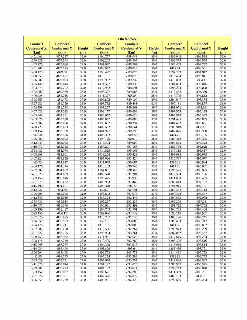
Okefenokee Lambert
Conformal X (km)
Lambert Conformal Y
(km) Height
(m)
Lambert Conformal X
(km)
Lambert Conformal Y
(km) Height
(m)
Lambert Conformal X
(km)
Lambert Conformal Y
(km) Height
(m) 1401.401 -877.287 36.0 1404.777 -888.047 36.0 1388.045 -894.538 36.0 1399.829 -877.544 36.0 1403.202 -888.305 36.0 1399.375 -894.585 36.0 1403.275 -878.866 27.0 1401.627 -888.562 36.0 1386.469 -894.792 36.0 1401.701 -879.123 27.0 1400.052 -888.819 36.0 1417.01 -893.581 36.0 1400.128 -879.38 30.0 1398.477 -889.075 36.0 1397.799 -894.842 36.0 1398.555 -879.637 36.0 1416.101 -888.073 36.0 1415.434 -893.841 36.0 1396.982 -879.893 36.0 1396.902 -889.332 36.0 1413.858 -894.1 37.0 1405.148 -880.444 36.0 1414.527 -888.332 36.0 1384.894 -895.046 36.0 1403.575 -880.702 37.0 1412.952 -888.591 36.0 1396.223 -895.098 36.0 1402.002 -880.959 36.0 1395.327 -889.588 33.0 1412.282 -894.359 36.0 1400.428 -881.216 36.0 1411.377 -888.85 38.0 1410.706 -894.618 36.0 1398.855 -881.473 36.0 1409.802 -889.109 29.0 1394.647 -895.354 36.0 1397.281 -881.729 36.0 1393.752 -889.843 32.0 1409.131 -894.877 36.0 1408.596 -881.764 36.0 1408.227 -889.368 36.0 1393.071 -895.61 36.0 1407.023 -882.023 36.0 1392.177 -890.099 36.0 1407.555 -895.135 36.0 1405.449 -882.281 36.0 1406.652 -889.626 36.0 1405.978 -895.393 36.0 1403.875 -882.538 27.0 1405.077 -889.883 37.0 1391.495 -895.865 36.0 1402.302 -882.796 27.0 1390.602 -890.354 38.0 1404.402 -895.651 36.0 1400.728 -883.053 30.0 1403.502 -890.141 37.0 1389.918 -896.12 36.0 1399.154 -883.309 27.0 1401.927 -890.398 37.0 1402.826 -895.908 36.0 1397.58 -883.566 31.0 1400.352 -890.655 36.0 1401.25 -896.165 36.0 1396.006 -883.822 36.0 1398.776 -890.912 36.0 1388.342 -896.375 36.0 1412.045 -883.083 36.0 1416.404 -889.909 36.0 1399.674 -896.422 37.0 1410.472 -883.342 36.0 1397.201 -891.168 36.0 1386.766 -896.629 36.0 1394.432 -884.078 36.0 1414.829 -890.168 36.0 1417.313 -895.417 36.0 1408.898 -883.601 36.0 1413.254 -890.428 36.0 1398.098 -896.679 36.0 1407.324 -883.859 36.0 1395.626 -891.424 36.0 1415.737 -895.677 36.0 1405.75 -884.117 36.0 1411.679 -890.687 38.0 1385.19 -896.884 36.0 1404.176 -884.374 36.0 1410.103 -890.945 37.0 1414.16 -895.937 36.0 1402.602 -884.632 36.0 1394.051 -891.68 38.0 1396.521 -896.935 36.0 1401.028 -884.889 36.0 1408.528 -891.204 36.0 1412.584 -896.196 36.0 1399.453 -885.146 36.0 1392.475 -891.936 36.0 1411.008 -896.455 36.0 1397.879 -885.402 36.0 1406.953 -891.462 36.0 1383.613 -897.137 36.0 1415.496 -884.401 27.0 1405.378 -891.72 38.0 1394.945 -897.191 36.0 1413.922 -884.66 30.0 1390.9 -892.191 38.0 1409.432 -896.713 36.0 1396.305 -885.658 31.0 1403.802 -891.978 37.0 1393.368 -897.447 36.0 1412.347 -884.919 32.0 1389.324 -892.446 37.0 1407.855 -896.972 36.0 1394.731 -885.914 27.0 1402.227 -892.235 36.0 1406.279 -897.23 36.0 1410.773 -885.178 27.0 1400.651 -892.492 36.0 1391.792 -897.702 36.0 1409.199 -885.437 36.0 1387.749 -892.701 36.0 1404.703 -897.488 36.0 1393.156 -886.17 36.0 1399.076 -892.749 36.0 1390.216 -897.957 36.0 1407.625 -885.695 36.0 1416.707 -891.745 36.0 1403.126 -897.745 36.0 1406.051 -885.953 36.0 1397.5 -893.005 36.0 1388.639 -898.212 36.0 1404.476 -886.211 36.0 1415.131 -892.005 36.0 1401.55 -898.002 36.0 1402.902 -886.468 36.0 1413.556 -892.264 36.0 1399.973 -898.259 36.0 1401.327 -886.725 36.0 1395.924 -893.261 37.0 1387.062 -898.467 36.0 1399.753 -886.982 36.0 1411.981 -892.523 38.0 1417.615 -897.254 36.0 1398.178 -887.239 36.0 1410.405 -892.782 38.0 1398.396 -898.516 36.0 1415.798 -886.237 37.0 1394.349 -893.517 38.0 1416.039 -897.514 36.0 1414.224 -886.496 36.0 1408.829 -893.04 36.0 1385.486 -898.721 36.0 1396.604 -887.495 27.0 1392.773 -893.773 36.0 1414.463 -897.773 36.0 1412.65 -886.755 27.0 1407.254 -893.299 36.0 1396.82 -898.772 36.0 1395.029 -887.751 27.0 1405.678 -893.557 36.0 1412.886 -898.033 36.0 1411.075 -887.014 27.0 1391.197 -894.028 36.0 1383.909 -898.975 36.0 1409.501 -887.273 30.0 1404.102 -893.814 36.0 1395.243 -899.028 36.0 1393.454 -888.007 34.0 1389.621 -894.283 36.0 1411.309 -898.291 36.0 1407.926 -887.531 36.0 1402.526 -894.072 36.0 1409.733 -898.55 36.0 1406.351 -887.789 36.0 1400.951 -894.329 36.0 1393.666 -899.284 36.0
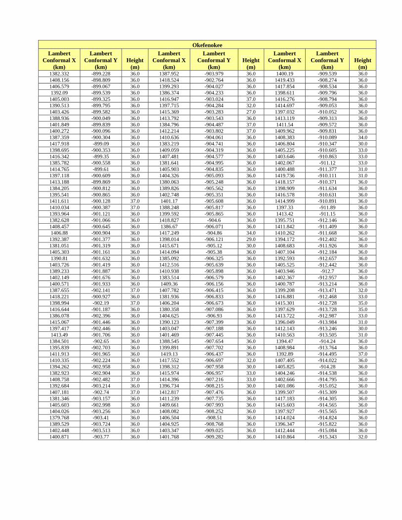
Okefenokee Lambert
Conformal X (km)
Lambert Conformal Y
(km) Height
(m)
Lambert Conformal X
(km)
Lambert Conformal Y
(km) Height
(m)
Lambert Conformal X
(km)
Lambert Conformal Y
(km) Height
(m) 1382.332 -899.228 36.0 1387.952 -903.979 36.0 1400.19 -909.539 36.0 1408.156 -898.809 36.0 1418.524 -902.764 36.0 1419.433 -908.274 36.0 1406.579 -899.067 36.0 1399.293 -904.027 36.0 1417.854 -908.534 36.0 1392.09 -899.539 36.0 1386.374 -904.233 36.0 1398.611 -909.796 36.0 1405.003 -899.325 36.0 1416.947 -903.024 37.0 1416.276 -908.794 36.0 1390.513 -899.795 36.0 1397.715 -904.284 32.0 1414.697 -909.053 36.0 1403.426 -899.582 36.0 1415.369 -903.283 27.0 1397.032 -910.052 36.0 1388.936 -900.049 36.0 1413.792 -903.543 36.0 1413.119 -909.313 36.0 1401.849 -899.839 36.0 1384.796 -904.487 37.0 1411.54 -909.572 36.0 1400.272 -900.096 36.0 1412.214 -903.802 37.0 1409.962 -909.831 36.0 1387.359 -900.304 36.0 1410.636 -904.061 36.0 1408.383 -910.089 34.0 1417.918 -899.09 36.0 1383.219 -904.741 36.0 1406.804 -910.347 30.0 1398.695 -900.353 36.0 1409.059 -904.319 36.0 1405.225 -910.605 33.0 1416.342 -899.35 36.0 1407.481 -904.577 36.0 1403.646 -910.863 33.0 1385.782 -900.558 36.0 1381.641 -904.995 36.0 1402.067 -911.12 33.0 1414.765 -899.61 36.0 1405.903 -904.835 36.0 1400.488 -911.377 31.0 1397.118 -900.609 36.0 1404.326 -905.093 36.0 1419.736 -910.111 31.0 1413.188 -899.869 36.0 1380.063 -905.248 36.0 1418.157 -910.371 36.0 1384.205 -900.812 36.0 1389.826 -905.562 36.0 1398.909 -911.634 36.0 1395.541 -900.865 36.0 1402.748 -905.351 36.0 1416.578 -910.631 36.0 1411.611 -900.128 37.0 1401.17 -905.608 36.0 1414.999 -910.891 36.0 1410.034 -900.387 37.0 1388.248 -905.817 36.0 1397.33 -911.89 36.0 1393.964 -901.121 36.0 1399.592 -905.865 36.0 1413.42 -911.15 36.0 1382.628 -901.066 36.0 1418.827 -904.6 36.0 1395.751 -912.146 36.0 1408.457 -900.645 36.0 1386.67 -906.071 36.0 1411.842 -911.409 36.0 1406.88 -900.904 36.0 1417.249 -904.86 34.0 1410.262 -911.668 36.0 1392.387 -901.377 36.0 1398.014 -906.121 29.0 1394.172 -912.402 36.0 1381.051 -901.319 36.0 1415.671 -905.12 30.0 1408.683 -911.926 36.0 1405.303 -901.161 36.0 1414.094 -905.38 36.0 1407.104 -912.184 36.0 1390.81 -901.632 36.0 1385.092 -906.325 36.0 1392.593 -912.657 36.0 1403.726 -901.419 36.0 1412.516 -905.639 36.0 1405.525 -912.442 36.0 1389.233 -901.887 36.0 1410.938 -905.898 36.0 1403.946 -912.7 36.0 1402.149 -901.676 36.0 1383.514 -906.579 36.0 1402.367 -912.957 36.0 1400.571 -901.933 36.0 1409.36 -906.156 36.0 1400.787 -913.214 36.0 1387.655 -902.141 37.0 1407.782 -906.415 36.0 1399.208 -913.471 32.0 1418.221 -900.927 36.0 1381.936 -906.833 36.0 1416.881 -912.468 33.0 1398.994 -902.19 37.0 1406.204 -906.673 36.0 1415.301 -912.728 35.0 1416.644 -901.187 36.0 1380.358 -907.086 36.0 1397.629 -913.728 35.0 1386.078 -902.396 36.0 1404.625 -906.93 36.0 1413.722 -912.987 33.0 1415.067 -901.446 36.0 1390.123 -907.399 36.0 1396.049 -913.984 31.0 1397.417 -902.446 36.0 1403.047 -907.188 36.0 1412.143 -913.246 30.0 1413.49 -901.706 36.0 1401.469 -907.445 36.0 1410.563 -913.505 31.0 1384.501 -902.65 36.0 1388.545 -907.654 36.0 1394.47 -914.24 36.0 1395.839 -902.703 36.0 1399.891 -907.702 36.0 1408.984 -913.764 36.0 1411.913 -901.965 36.0 1419.13 -906.437 36.0 1392.89 -914.495 37.0 1410.335 -902.224 36.0 1417.552 -906.697 32.0 1407.405 -914.022 36.0 1394.262 -902.958 36.0 1398.312 -907.958 30.0 1405.825 -914.28 36.0 1382.923 -902.904 36.0 1415.974 -906.957 33.0 1404.246 -914.538 36.0 1408.758 -902.482 37.0 1414.396 -907.216 33.0 1402.666 -914.795 36.0 1392.684 -903.214 36.0 1396.734 -908.215 30.0 1401.086 -915.052 36.0 1407.181 -902.74 37.0 1412.817 -907.476 36.0 1399.507 -915.309 36.0 1381.346 -903.157 36.0 1411.239 -907.735 36.0 1417.183 -914.305 36.0 1405.603 -902.998 36.0 1409.661 -907.993 36.0 1415.603 -914.565 36.0 1404.026 -903.256 36.0 1408.082 -908.252 36.0 1397.927 -915.565 36.0 1379.768 -903.41 36.0 1406.504 -908.51 36.0 1414.024 -914.824 36.0 1389.529 -903.724 36.0 1404.925 -908.768 36.0 1396.347 -915.822 36.0 1402.448 -903.513 36.0 1403.347 -909.025 36.0 1412.444 -915.084 36.0 1400.871 -903.77 36.0 1401.768 -909.282 36.0 1410.864 -915.343 32.0
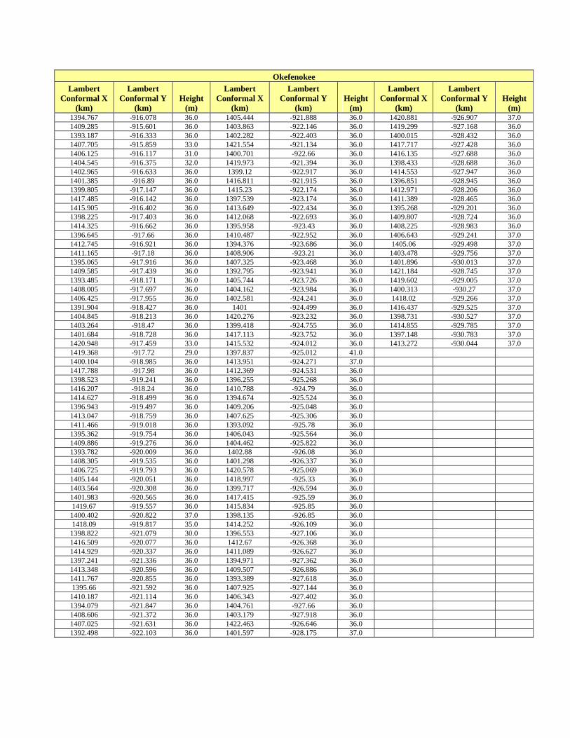
Okefenokee
Lambert Conformal X
(km)
Lambert Conformal Y
(km) Height
(m)
Lambert Conformal X
(km)
Lambert Conformal Y
(km) Height
(m)
Lambert Conformal X
(km)
Lambert Conformal Y
(km) Height
(m) 1394.767 -916.078 36.0 1405.444 -921.888 36.0 1420.881 -926.907 37.0 1409.285 -915.601 36.0 1403.863 -922.146 36.0 1419.299 -927.168 36.0 1393.187 -916.333 36.0 1402.282 -922.403 36.0 1400.015 -928.432 36.0 1407.705 -915.859 33.0 1421.554 -921.134 36.0 1417.717 -927.428 36.0 1406.125 -916.117 31.0 1400.701 -922.66 36.0 1416.135 -927.688 36.0 1404.545 -916.375 32.0 1419.973 -921.394 36.0 1398.433 -928.688 36.0 1402.965 -916.633 36.0 1399.12 -922.917 36.0 1414.553 -927.947 36.0 1401.385 -916.89 36.0 1416.811 -921.915 36.0 1396.851 -928.945 36.0 1399.805 -917.147 36.0 1415.23 -922.174 36.0 1412.971 -928.206 36.0 1417.485 -916.142 36.0 1397.539 -923.174 36.0 1411.389 -928.465 36.0 1415.905 -916.402 36.0 1413.649 -922.434 36.0 1395.268 -929.201 36.0 1398.225 -917.403 36.0 1412.068 -922.693 36.0 1409.807 -928.724 36.0 1414.325 -916.662 36.0 1395.958 -923.43 36.0 1408.225 -928.983 36.0 1396.645 -917.66 36.0 1410.487 -922.952 36.0 1406.643 -929.241 37.0 1412.745 -916.921 36.0 1394.376 -923.686 36.0 1405.06 -929.498 37.0 1411.165 -917.18 36.0 1408.906 -923.21 36.0 1403.478 -929.756 37.0 1395.065 -917.916 36.0 1407.325 -923.468 36.0 1401.896 -930.013 37.0 1409.585 -917.439 36.0 1392.795 -923.941 36.0 1421.184 -928.745 37.0 1393.485 -918.171 36.0 1405.744 -923.726 36.0 1419.602 -929.005 37.0 1408.005 -917.697 36.0 1404.162 -923.984 36.0 1400.313 -930.27 37.0 1406.425 -917.955 36.0 1402.581 -924.241 36.0 1418.02 -929.266 37.0 1391.904 -918.427 36.0 1401 -924.499 36.0 1416.437 -929.525 37.0 1404.845 -918.213 36.0 1420.276 -923.232 36.0 1398.731 -930.527 37.0 1403.264 -918.47 36.0 1399.418 -924.755 36.0 1414.855 -929.785 37.0 1401.684 -918.728 36.0 1417.113 -923.752 36.0 1397.148 -930.783 37.0 1420.948 -917.459 33.0 1415.532 -924.012 36.0 1413.272 -930.044 37.0 1419.368 -917.72 29.0 1397.837 -925.012 41.0 1400.104 -918.985 36.0 1413.951 -924.271 37.0 1417.788 -917.98 36.0 1412.369 -924.531 36.0 1398.523 -919.241 36.0 1396.255 -925.268 36.0 1416.207 -918.24 36.0 1410.788 -924.79 36.0 1414.627 -918.499 36.0 1394.674 -925.524 36.0 1396.943 -919.497 36.0 1409.206 -925.048 36.0 1413.047 -918.759 36.0 1407.625 -925.306 36.0 1411.466 -919.018 36.0 1393.092 -925.78 36.0 1395.362 -919.754 36.0 1406.043 -925.564 36.0 1409.886 -919.276 36.0 1404.462 -925.822 36.0 1393.782 -920.009 36.0 1402.88 -926.08 36.0 1408.305 -919.535 36.0 1401.298 -926.337 36.0 1406.725 -919.793 36.0 1420.578 -925.069 36.0 1405.144 -920.051 36.0 1418.997 -925.33 36.0 1403.564 -920.308 36.0 1399.717 -926.594 36.0 1401.983 -920.565 36.0 1417.415 -925.59 36.0 1419.67 -919.557 36.0 1415.834 -925.85 36.0 1400.402 -920.822 37.0 1398.135 -926.85 36.0 1418.09 -919.817 35.0 1414.252 -926.109 36.0 1398.822 -921.079 30.0 1396.553 -927.106 36.0 1416.509 -920.077 36.0 1412.67 -926.368 36.0 1414.929 -920.337 36.0 1411.089 -926.627 36.0 1397.241 -921.336 36.0 1394.971 -927.362 36.0 1413.348 -920.596 36.0 1409.507 -926.886 36.0 1411.767 -920.855 36.0 1393.389 -927.618 36.0 1395.66 -921.592 36.0 1407.925 -927.144 36.0 1410.187 -921.114 36.0 1406.343 -927.402 36.0 1394.079 -921.847 36.0 1404.761 -927.66 36.0 1408.606 -921.372 36.0 1403.179 -927.918 36.0 1407.025 -921.631 36.0 1422.463 -926.646 36.0 1392.498 -922.103 36.0 1401.597 -928.175 37.0

Wolf Island Lambert
Conformal X (km)
Lambert Conformal Y
(km) Height
(m)
Lambert Conformal X
(km)
Lambert Conformal Y
(km) Height
(m)
Lambert Conformal X
(km)
Lambert Conformal Y
(km) Height
(m) 1485.848 -828.138 1.0 1485.225 -829.19 1.0 1486.007 -829.054 1.0 1486.789 -828.918 3.0 1487.571 -828.781 2.0 1488.353 -828.645 1.0 1485.385 -830.106 1.0 1489.135 -828.509 1.0 1486.167 -829.97 1.0 1486.949 -829.834 1.0 1487.731 -829.697 1.0 1488.513 -829.561 1.0 1489.295 -829.424 1.0 1486.327 -830.886 1.0 1487.109 -830.749 1.0 1487.891 -830.613 1.0 1488.673 -830.476 1.0 1489.455 -830.34 1.0 1486.486 -831.801 1.0 1487.268 -831.665 1.0 1488.051 -831.529 1.0 1488.833 -831.392 1.0 1489.615 -831.256 1.0 1487.428 -832.581 1.0 1488.21 -832.444 1.0 1488.993 -832.308 1.0 1489.775 -832.171 1.0 1488.53 -834.276 1.0 1488.69 -835.192 1.0 1489.472 -835.055 1.0
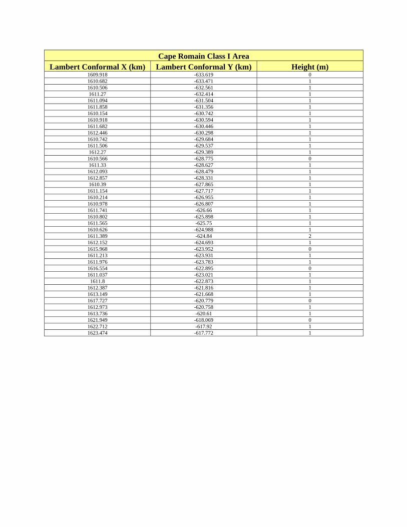
Cape Romain Class I Area
Lambert Conformal X (km) Lambert Conformal Y (km) Height (m) 1609.918 -633.619 0 1610.682 -633.471 1 1610.506 -632.561 1 1611.27 -632.414 1
1611.094 -631.504 1 1611.858 -631.356 1 1610.154 -630.742 1 1610.918 -630.594 1 1611.682 -630.446 1 1612.446 -630.298 1 1610.742 -629.684 1 1611.506 -629.537 1 1612.27 -629.389 1
1610.566 -628.775 0 1611.33 -628.627 1
1612.093 -628.479 1 1612.857 -628.331 1 1610.39 -627.865 1
1611.154 -627.717 1 1610.214 -626.955 1 1610.978 -626.807 1 1611.741 -626.66 1 1610.802 -625.898 1 1611.565 -625.75 1 1610.626 -624.988 1 1611.389 -624.84 2 1612.152 -624.693 1 1615.968 -623.952 0 1611.213 -623.931 1 1611.976 -623.783 1 1616.554 -622.895 0 1611.037 -623.021 1
1611.8 -622.873 1 1612.387 -621.816 1 1613.149 -621.668 1 1617.727 -620.779 0 1612.973 -620.758 1 1613.736 -620.61 1 1621.949 -618.069 0 1622.712 -617.92 1 1623.474 -617.772 1
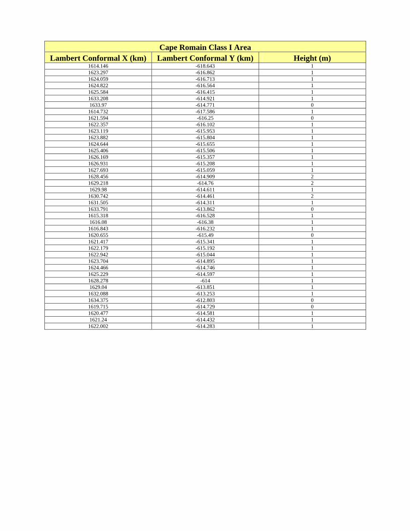
Cape Romain Class I Area Lambert Conformal X (km) Lambert Conformal Y (km) Height (m)
1614.146 -618.643 1 1623.297 -616.862 1 1624.059 -616.713 1 1624.822 -616.564 1 1625.584 -616.415 1 1633.208 -614.921 1 1633.97 -614.771 0
1614.732 -617.586 1 1621.594 -616.25 0 1622.357 -616.102 1 1623.119 -615.953 1 1623.882 -615.804 1 1624.644 -615.655 1 1625.406 -615.506 1 1626.169 -615.357 1 1626.931 -615.208 1 1627.693 -615.059 1 1628.456 -614.909 2 1629.218 -614.76 2 1629.98 -614.611 1
1630.742 -614.461 2 1631.505 -614.311 1 1633.791 -613.862 0 1615.318 -616.528 1 1616.08 -616.38 1
1616.843 -616.232 1 1620.655 -615.49 0 1621.417 -615.341 1 1622.179 -615.192 1 1622.942 -615.044 1 1623.704 -614.895 1 1624.466 -614.746 1 1625.229 -614.597 1 1628.278 -614 1 1629.04 -613.851 1
1632.088 -613.253 1 1634.375 -612.803 0 1619.715 -614.729 0 1620.477 -614.581 1 1621.24 -614.432 1
1622.002 -614.283 1
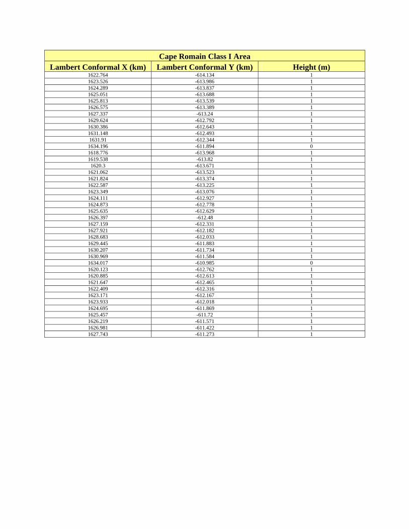
Cape Romain Class I Area
Lambert Conformal X (km) Lambert Conformal Y (km) Height (m) 1622.764 -614.134 1 1623.526 -613.986 1 1624.289 -613.837 1 1625.051 -613.688 1 1625.813 -613.539 1 1626.575 -613.389 1 1627.337 -613.24 1 1629.624 -612.792 1 1630.386 -612.643 1 1631.148 -612.493 1 1631.91 -612.344 1
1634.196 -611.894 0 1618.776 -613.968 1 1619.538 -613.82 1
1620.3 -613.671 1 1621.062 -613.523 1 1621.824 -613.374 1 1622.587 -613.225 1 1623.349 -613.076 1 1624.111 -612.927 1 1624.873 -612.778 1 1625.635 -612.629 1 1626.397 -612.48 1 1627.159 -612.331 1 1627.921 -612.182 1 1628.683 -612.033 1 1629.445 -611.883 1 1630.207 -611.734 1 1630.969 -611.584 1 1634.017 -610.985 0 1620.123 -612.762 1 1620.885 -612.613 1 1621.647 -612.465 1 1622.409 -612.316 1 1623.171 -612.167 1 1623.933 -612.018 1 1624.695 -611.869 1 1625.457 -611.72 1 1626.219 -611.571 1 1626.981 -611.422 1 1627.743 -611.273 1
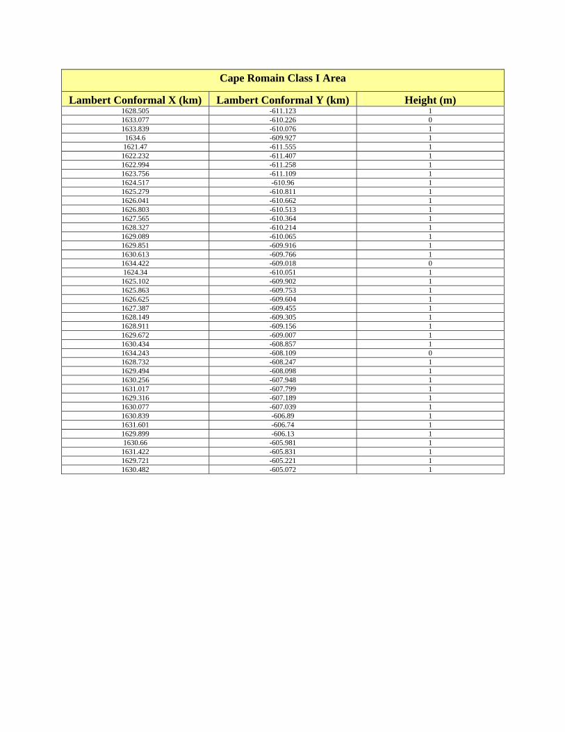
Cape Romain Class I Area
Lambert Conformal X (km) Lambert Conformal Y (km) Height (m) 1628.505 -611.123 1 1633.077 -610.226 0 1633.839 -610.076 1
1634.6 -609.927 1 1621.47 -611.555 1
1622.232 -611.407 1 1622.994 -611.258 1 1623.756 -611.109 1 1624.517 -610.96 1 1625.279 -610.811 1 1626.041 -610.662 1 1626.803 -610.513 1 1627.565 -610.364 1 1628.327 -610.214 1 1629.089 -610.065 1 1629.851 -609.916 1 1630.613 -609.766 1 1634.422 -609.018 0 1624.34 -610.051 1
1625.102 -609.902 1 1625.863 -609.753 1 1626.625 -609.604 1 1627.387 -609.455 1 1628.149 -609.305 1 1628.911 -609.156 1 1629.672 -609.007 1 1630.434 -608.857 1 1634.243 -608.109 0 1628.732 -608.247 1 1629.494 -608.098 1 1630.256 -607.948 1 1631.017 -607.799 1 1629.316 -607.189 1 1630.077 -607.039 1 1630.839 -606.89 1 1631.601 -606.74 1 1629.899 -606.13 1 1630.66 -605.981 1
1631.422 -605.831 1 1629.721 -605.221 1 1630.482 -605.072 1
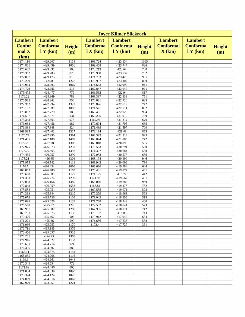
Joyce Kilmer Slickrock
Lambert Conformal X (km)
Lambert Conformal Y (km)
Height
(m)
Lambert Conformal X (km)
Lambert Conformal Y (km)
Height
(m)
Lambert Conformal
X (km)
Lambert Conformal Y (km)
Height
(m)
1174.116 -429.607 1154 1168.724 -423.854 1065 1174.861 -429.499 1056 1169.468 -423.747 836 1175.607 -429.391 903 1170.213 -423.64 700 1176.352 -429.283 820 1170.958 -423.532 782 1177.097 -429.175 818 1171.703 -423.425 961 1173.239 -428.8 1278 1173.937 -423.102 809 1173.984 -428.693 1069 1174.682 -422.995 941 1174.729 -428.585 913 1167.847 -423.047 991 1175.475 -428.477 776 1168.592 -422.94 817 1176.22 -428.369 788 1169.337 -422.833 751
1176.965 -428.262 750 1170.081 -422.726 635 1172.362 -427.994 1327 1170.826 -422.619 772 1173.107 -427.887 1085 1171.571 -422.511 882 1173.852 -427.779 985 1168.461 -422.026 954 1174.597 -427.671 934 1169.205 -421.919 739 1175.342 -427.563 978 1169.95 -421.812 620 1176.088 -427.456 982 1170.694 -421.705 635 1176.833 -427.348 824 1171.439 -421.597 700 1169.995 -427.402 1317 1172.184 -421.49 865 1170.74 -427.295 1394 1168.329 -421.113 943
1171.485 -427.188 1487 1169.074 -421.005 742 1172.23 -427.08 1308 1169.818 -420.898 505
1172.975 -426.973 1237 1170.563 -420.791 558 1173.72 -426.865 1336 1171.307 -420.684 538
1174.465 -426.757 1290 1172.052 -420.576 686 1175.21 -426.65 1304 1168.198 -420.199 946
1175.955 -426.542 1111 1168.942 -420.092 760 1176.7 -426.434 1066 1169.686 -419.984 644
1169.863 -426.489 1189 1170.431 -419.877 491 1170.608 -426.381 1127 1171.175 -419.77 442 1171.353 -426.274 1299 1171.92 -419.662 491 1172.098 -426.166 1380 1168.066 -419.285 959 1172.843 -426.059 1553 1168.81 -419.178 752 1173.588 -425.951 1336 1169.555 -419.071 528 1174.333 -425.844 1219 1170.299 -418.963 598 1175.078 -425.736 1109 1171.043 -418.856 515 1175.823 -425.628 1133 1171.788 -418.749 400 1176.568 -425.52 1226 1172.532 -418.641 523 1168.987 -425.682 1280 1167.935 -418.371 712 1169.731 -425.575 1136 1170.167 -418.05 743 1170.476 -425.467 906 1170.912 -417.942 684 1171.221 -425.36 999 1171.656 -417.835 538 1171.966 -425.253 1170 1172.4 -417.727 361 1172.711 -425.145 1376 1173.456 -425.037 1318 1174.201 -424.93 1369 1174.946 -424.822 1152 1175.691 -424.714 924 1176.436 -424.607 882 1168.11 -424.875 1151
1168.855 -424.768 1116 1169.6 -424.661 1044
1170.345 -424.554 772 1171.09 -424.446 866
1171.834 -424.339 1090 1173.324 -424.124 1020 1174.069 -424.016 1067 1167.979 -423.961 1224
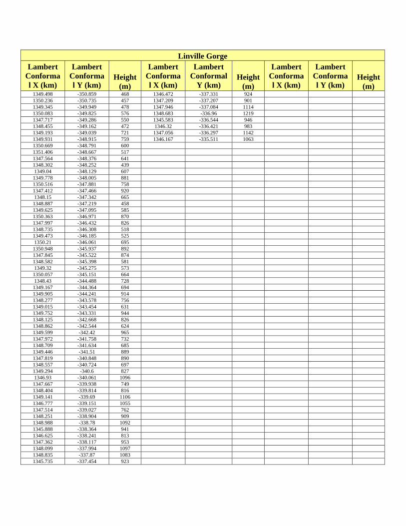
Linville Gorge
Lambert Conformal X (km)
Lambert Conformal Y (km)
Height
(m)
Lambert Conformal X (km)
Lambert Conformal
Y (km)
Height
(m)
Lambert Conformal X (km)
Lambert Conformal Y (km)
Height
(m) 1349.498 -350.859 468 1346.472 -337.331 924 1350.236 -350.735 457 1347.209 -337.207 901 1349.345 -349.949 478 1347.946 -337.084 1114 1350.083 -349.825 576 1348.683 -336.96 1219 1347.717 -349.286 550 1345.583 -336.544 946 1348.455 -349.162 472 1346.32 -336.421 983 1349.193 -349.039 721 1347.056 -336.297 1142 1349.931 -348.915 759 1346.167 -335.511 1063 1350.669 -348.791 600 1351.406 -348.667 517 1347.564 -348.376 641 1348.302 -348.252 439 1349.04 -348.129 607
1349.778 -348.005 881 1350.516 -347.881 758 1347.412 -347.466 920 1348.15 -347.342 665
1348.887 -347.219 458 1349.625 -347.095 585 1350.363 -346.971 870 1347.997 -346.432 826 1348.735 -346.308 518 1349.473 -346.185 525 1350.21 -346.061 695
1350.948 -345.937 892 1347.845 -345.522 874 1348.582 -345.398 581 1349.32 -345.275 573
1350.057 -345.151 664 1348.43 -344.488 728
1349.167 -344.364 694 1349.905 -344.241 914 1348.277 -343.578 756 1349.015 -343.454 631 1349.752 -343.331 944 1348.125 -342.668 826 1348.862 -342.544 624 1349.599 -342.42 965 1347.972 -341.758 732 1348.709 -341.634 685 1349.446 -341.51 889 1347.819 -340.848 890 1348.557 -340.724 697 1349.294 -340.6 827 1346.93 -340.061 1096
1347.667 -339.938 749 1348.404 -339.814 816 1349.141 -339.69 1106 1346.777 -339.151 1055 1347.514 -339.027 762 1348.251 -338.904 909 1348.988 -338.78 1092 1345.888 -338.364 941 1346.625 -338.241 813 1347.362 -338.117 953 1348.099 -337.994 1097 1348.835 -337.87 1083 1345.735 -337.454 923