Background Information Document for the Revision of 40 CFR ...
260
For assistance accessing this document or additional information, please contact [email protected]. Draft Technical Report CONSIDERATIONS RELATED TO POST CLOSURE MONITORING OF URANIUM IN-SITU LEACH/IN-SITU RECOVERY (ISL/ISR) SITES Background Information Document for the Revision of 40 CFR Part 192 Radiation Protection Division Office of Air and Radiation U.S. Environmental Protection Agency Revision 8 September 2014 EPA-402-D-14-001
-
Upload
khangminh22 -
Category
Documents
-
view
0 -
download
0
Transcript of Background Information Document for the Revision of 40 CFR ...

For assistance accessing this document or additional information, please contact [email protected].
Draft Technical Report
CONSIDERATIONS RELATED TO POST CLOSURE MONITORING OF URANIUM IN-SITU LEACH/IN-SITU RECOVERY (ISL/ISR) SITES
Background Information Document for the Revision of 40 CFR Part 192
Radiation Protection Division Office of Air and Radiation
U.S. Environmental Protection Agency
Revision 8 September 2014
EPA-402-D-14-001

TABLE OF CONTENTS Acronyms and Abbreviations ........................................................................................................ ix Overview ..........................................................................................................................................1
Background ..........................................................................................................................1 Overview of Report Contents ..............................................................................................2
1.0 Introduction ..........................................................................................................................4 1.1 Background versus Baseline Wells ..........................................................................7 1.2 ISR Facilities in the United States ...........................................................................9
2.0 Resource Conservation and Recovery Act ........................................................................14 2.1 Summary ................................................................................................................14 2.2 Ground Water Monitoring Requirements for Treatment, Storage, and
Disposal Facilities ..................................................................................................15 2.2.1 Overview ....................................................................................................15 2.2.2 Permitted Facilities ....................................................................................15 2.2.3 Detection Monitoring .................................................................................16 2.2.4 Compliance Monitoring .............................................................................17 2.2.5 Corrective Action .......................................................................................17
2.3 Application to ISR Facilities ..................................................................................18 3.0 Ground Water Monitoring at ISR Facilities .......................................................................20
3.1 Overview ................................................................................................................20 3.2 Pre-operational Monitoring (Phase 1) ....................................................................21 3.3 The ISR Leaching Process (Phase 2) .....................................................................22
3.3.1 Excursions during Operations ....................................................................24 3.4 Post-operational Monitoring (Phases 3 through 5) ................................................30 3.5 Selection of Parameters to Be Used in Ground Water Sampling Programs ..........31
3.5.1 Regulated Constituents ..............................................................................31 3.5.2 Summary of Species Potentially Required for Compliance
Monitoring – Tiered Approach ..................................................................39 3.5.3 Well Construction and Low-Flow Sampling Methodologies ....................42 3.5.4 Species Required for Geochemical Modeling ...........................................45 3.5.5 Species Required for Excursion Monitoring..............................................48 3.5.6 Case History – Evolution of Constituent Monitoring List .........................49 3.5.7 Formal Approach to Acceptable Restoration .............................................50
4.0 Technical Considerations for ISR Ground Water Monitoring ...........................................54 4.1 Uranium Geology...................................................................................................54
4.1.1 Formation of Uranium Containing Ore Deposits.......................................55 4.2 Aquifer Exemption Requirement ...........................................................................59 4.3 Establishing Baseline Conditions ..........................................................................59
4.3.1 Variability in Baseline Measurements .......................................................64 4.4 Extraction Operations Phase ..................................................................................68 4.5 Post-extraction Phase .............................................................................................70 4.6 Factors Affecting Post-mining Time Frames and Wellfield Stability ...................70 4.7 Modeling ................................................................................................................73
Draft Technical Report ii Revised Draft – September 2014
4.7.1 Objectives and Conceptual Model Development ......................................73 4.7.2 Ground Water Flow and Contaminant Transport Modeling ......................75 4.7.3 Geochemical Modeling ..............................................................................77 4.7.4 Demonstrating Long-term Stability of Restored ISR Wellfields –
Long-Term Monitoring and Geochemical Modeling ................................91 5.0 Active/Existing ISR Facilities: Monitoring Issues ............................................................94
5.1 Ground Water Baseline: Case Studies ...................................................................94 5.2 Wellfield Restoration .............................................................................................96 5.3 Wellfield Restoration: Case Study .........................................................................97
6.0 Issues Associated with Establishment of Post-restoration Steady State ............................99 6.1 Post-restoration Stability Monitoring ....................................................................99 6.2 Factors That Affect Time Frames for Post-mining Monitoring...........................100
6.2.1 Fate and Transport Processes ...................................................................100 6.2.2 Natural Attenuation Processes .................................................................103
6.3 Geochemically Based Restoration Techniques ....................................................109 6.4 Monitored Natural Attenuation ............................................................................110
6.4.1 Tiered Approach to Assessing Suitability of Monitored Natural Attenuation ...............................................................................................112
6.4.2 First-Order Attenuation Rate Determination ...........................................112 7.0 Statistical Analyses to Compare Pre- and Post-ISR Conditions ......................................115
7.1 Determine Baseline Characteristics .....................................................................119 7.1.1 Design for Baseline Sampling .................................................................122 7.1.2 Selection of Baseline Monitoring Wells ..................................................123 7.1.3 Determining the Number of Baseline Samples ........................................126 7.1.4 Summary ..................................................................................................130
7.2 Determining the Number of Monitoring Wells Required to Detect Noncompliance ....................................................................................................136 7.2.1 Determining the Number of Monitoring Wells based on
Hypergeometric Sampling .......................................................................136 7.2.2 An Alternative Graduated Approach to Hypergeometric Sampling ........146 7.2.3 Determining Connectivity of the Wellfield .............................................160
7.3 Hypothesis Testing and Data Quality Objectives ................................................162 7.3.1 Decision Errors and Confidence Levels ..................................................164 7.3.2 Hypothesis Tests for Comparisons with Baseline ...................................165 7.3.3 Selecting a Test Form ..............................................................................168 7.3.4 Hypothesis Tests for Detecting Trends ....................................................170
7.4 Selecting the Statistical Approach – Parametric Versus Nonparametric Methods................................................................................................................172 7.4.1 Determining If Data Have a Normal Distribution ...................................173 7.4.2 The Shapiro-Wilk W Test ........................................................................173 7.4.3 The Studentized Range Test ....................................................................173
7.5 Outlier Detection ..................................................................................................174 7.5.1 Parametric Tolerance Limits for Outliers ................................................175 7.5.2 Calculating an Upper Tolerance Limit ....................................................176
7.6 Determining the Number of Samples per Well ....................................................178
Draft Technical Report iii Revised Draft – September 2014

7.6.1 Same Sample Sizes (n=m) and Same Standard Deviation (σ1=σ2) .........179 7.6.2 Different Sample Sizes (n≠m), Same Standard Deviations (σ1=σ2) .......180 7.6.3 Different Sample Sizes (n≠m) and Different Standard Deviations
(σ1≠σ2) .....................................................................................................180 7.7 Statistical Methods for Trends and Seasonality ...................................................181
7.7.1 Adjusting for Seasonality .........................................................................182 7.7.2 Using Trend Tests to Determine Stability ...............................................184
7.8 Analysis of Post-restoration Trends at ISR Sites .................................................199 7.8.1 Trend Analysis by Well ...........................................................................199 7.8.2 Pooled Trend Analysis .............................................................................210
7.9 Verify that Contaminants and Hazardous Constituent Concentrations are Below Required Restoration Levels ....................................................................214 7.9.1 Parametric Method for Determining Compliance of Individual Wells ...215 7.9.2 Nonparametric Tests for Comparing Baseline and Post-restoration
Conditions ................................................................................................220 7.10 ProUCL Software for Statistical Analysis ...........................................................223 7.11 Summary of Statistical Approaches .....................................................................224
8.0 Summary of Post-closure Performance Issues .................................................................226 8.1 Designing the Monitoring Program to Allow Reliable Baseline Conditions
to be Established Prior to Active Mining .............................................................226 8.2 Determining that the Ground Water Chemistry has Reached Steady State
and Restoration Processes can be Discontinued ..................................................228 8.3 Post-restoration Stability Monitoring ..................................................................229
9.0 References ........................................................................................................................232
ATTACHMENTS
Attachment A: Development of Ground Water Baseline for Dewey-Burdock ISL/ISR Site in South Dakota
Attachment B: Post-restoration Stability Monitoring Case Histories
Attachment C: Aquifer Restoration (Extracted from NRC 2009, Section 2.11.5)
Attachment D: Instructions and Examples for Statistical Calculations
Attachment E: Statistical Tables
Attachment F: Detailed Results of Regression Trend Analysis by Analyte and Mine Unit
Attachment G: Using Trend Tests to Determine Stability
Attachment H: Glossary of Terms
Draft Technical Report iv Revised Draft – September 2014
LIST OF TABLES
Table 1-1. NRC-Licensed ISR Facilities as of September 2011 ...............................................9 Table 1-2. Uranium Recovery Facility Applications, Reviews, and Letters of Intent by
NRC .......................................................................................................................11 Table 1-3. List of In-Situ Uranium Mines in Texas ................................................................13 Table 3-1. Wells on Excursion at Christensen Ranch – 2Q 2011 ...........................................30 Table 3-2. Ground Water Species Identified in EPA Regulations That May
Require Monitoring at ISR Facilities .....................................................................35 Table 3-3. Comparison of Ground Water Parameter Measurements Established by
Various Regulators with Actual Field Measurements from Dewey-Burdock Site .........................................................................................................................39
Table 3-4. Parameters for Solid Phase Characterization .........................................................47 Table 3-5. Basis for Inclusion of Various Analytes in ISR
Ground Water Monitoring Program .......................................................................51 Table 4-1. Summary of Commonly Applied Geochemical Modeling Codes .........................86 Table 5-1. Baseline Water Quality Data for Zamzow PAA-1 ................................................95 Table 5-2. Ground Water Chemistry of Texas In-Situ Uranium Production
Authorization Areas ...............................................................................................98 Table 6-1. Post-restoration and Stability Monitoring Periods ...............................................100 Table 7-1. Outline of the Statistical Procedures used in Phases 1, 4, and 5 ..........................117 Table 7-2. Summary Statistics for Population Coefficient of Variation (cv) of Baseline
Parameters at Nine ISR Sites ...............................................................................130 Table 7-3. Baseline Statistics and Number of Samples Required at Christensen Mine
Unit 6 for the Relative Standard Error of the Baseline Mean to Be Less Than P% for 35 Analytes with Summary Statistics for U and Ra-226 ................132
Table 7-4. Wellfield Characteristics and Comparison of Actual and Target Baseline Sample Size at Nine ISR Production Units..........................................................134
Table 7-5. Number of Samples Required at Nine Production Units for Relative Standard Error of U and Ra-226 Mean Baseline Concentrations to Be Less Than ±P% .............................................................................................................135
Table 7-6. Parameter Definitions for the Hypergeometric Distribution ...............................139 Table 7-7. Minimum Value of N with Prob {Q ≤ q | x=0, M, N} ≥ 0.95 .............................142 Table 7-8. Minimum Value of N with Prob {Q ≤ q | x=1, M, N} ≥ 0.95 .............................144 Table 7-9. Ratio of Monitor Wells to Production Wells .......................................................156 Table 7-10. Number of Monitoring Wells Required for Five Design Options for a
Production Unit with 181 Wells in 5-spot Pattern (Posterior Probability=90%) .................................................................................................156
Draft Technical Report v Revised Draft – September 2014

Table 7-11. Number of Monitoring Wells Required for Five Design Options for a Production Unit with 181 Wells in 5-spot Pattern (Posterior Probability=95%) .................................................................................................156
Table 7-12. Number of Monitoring Wells Required for Four Design Options for a Production Unit with 162 Wells in 7-spot Pattern (Posterior Probability=90%) .................................................................................................157
Table 7-13. Number of Monitoring Wells Required for Four Design Options for a Production Unit with 162 Wells in 7-spot Pattern (Posterior Probability=95%) .................................................................................................157
Table 7-14. Number of Monitoring Wells Required for Posterior Probability of 90% that at Least P% of the Well Zones Demonstrate Compliance ...................................158
Table 7-15. Number of Monitoring Wells Required for Posterior Probability of 95% that at Least P% of the Well Zones Demonstrate Compliance ...................................159
Table 7-16. Hypothesis Testing: Type I and Type II Errors ...................................................164 Table 7-17. Critical Values for the Studentized Range Test ...................................................174 Table 7-18. One-Sided Upper Tolerance Limit Factors with g% Coverage
for Selected Values of N ......................................................................................177 Table 7-19. Number of Quarterly Samples Required for 90% Probability of Detecting
Slope Using a Mann-Kendall or Regression Trend Test .....................................187 Table 7-20. Number of Quarterly Samples Required for 95% Probability of Detecting
Slope Using a Mann-Kendall or Regression Trend Test .....................................188 Table 7-21. Number of Quarterly Samples Required for 99% Probability of Detecting
Slope Using a Mann-Kendall or Regression Trend Test .....................................189 Table 7-22. Probability of Detecting a Trend with 12 Quarterly Samples..............................191 Table 7-23. Probability of Detecting a Trend with 20 Quarterly Samples..............................192 Table 7-24. Probability of Detecting a Trend with 32 Quarterly Samples..............................193 Table 7-25. Number of Samples and Number of Years Required for 95% Chance of
Detection Using Regression or Mann-Kendall Test ............................................195 Table 7-26. Regression Statistics for Example in Figure 7-16................................................200 Table 7-27. Summary of Trend Analysis at Four* ISR Sites ..................................................206 Table 7-28. Mean Slope and Variability Estimates with 95% Confidence Interval for the
Mean (LCL to UCL) ............................................................................................207 Table 7-29. Summary of Significant Trends in Pooled Trend Analysis .................................214 Table 7-30. Significant Positive and Negative Trends Identified using Pooled Trend
Analysis................................................................................................................214 Table 7-31. Critical Values of the Student’s t-Distribution ....................................................217
Draft Technical Report vi Revised Draft – September 2014
LIST OF FIGURES
Figure 1-1. Historical U.S. Uranium Production after World War II .........................................5 Figure 1-2. In-situ Uranium Recovery – Process Flow Diagram ...............................................6 Figure 3-1. Variation of Typical Ground Water Constituent over Time ..................................21 Figure 3-2. Idealized Schematic Cross Section to Illustrate Ore-Zone Geology and
Lixiviant Migration from an Injection Well to a Production Well (NRC 2009) ......................................................................................................................22
Figure 3-3. Schematic Diagram of a Wellfield Showing Typical Injection/Production Well Patterns, Monitoring Wells, Manifold Buildings, and Pipelines (NRC 2009) ......................................................................................................................23
Figure 3-4. Wellheads and Header House, Smith Ranch, Converse County, Wyoming .........24 Figure 3-5. Alkalinity (mg/L) Variation during Excursion of Crow Butte ..............................28 Figure 3-6. Conductivity (µmho/cm) Variation during Excursion of Crow Butte ...................28 Figure 3-7. Chloride (mg/L) Variation during Excursion of Crow Butte.................................29 Figure 3-8. Cross Section of a Typical Injection, Production, or Monitoring Well .................44 Figure 3-9. Major Chemical Reactions Involved in Uranium Recovery and Restoration........46 Figure 4-1. Uranium Resource Areas of the United States ......................................................54 Figure 4-2. Pending, Licensed, and Active ISL Operations .....................................................55 Figure 4-3. Three-Dimensional Depiction of Uranium Ore Deposited in Paleochannels ........56 Figure 4-4. Schematic Diagrams of the Different Geometries for Tabular, Roll-front,
Fault Displaced, and Remnant Ore ........................................................................56 Figure 4-5. Conceptual Cross-Section of Uranium Roll-front Deposits ..................................57 Figure 4-6. Conceptual Model of Uranium Roll-front Deposit ................................................58 Figure 4-7. Well and Production Zone Locations and Baseline Concentrations of TDS,
Uranium, and Radium –Wellfield H-E ..................................................................63 Figure 4-8. Baseline Uranium Concentrations at the Rosita ISR Facility ................................64 Figure 4-9. Schematic Diagram of a Wellfield Showing Typical Injection/Production
Well Patterns, Monitoring Wells ...........................................................................68 Figure 4-10. Example of MODFLOW Predicted Potentiometric Surface during Active
Mining ....................................................................................................................69 Figure 4-11. Example of MODPATH Predicted Flow Paths During Active Mining ...............69 Figure 4-12. Example of PHT3D Predicted Post-mining Uraninite Concentrations .................71 Figure 7-1. Ore Zone Outline and Well Locations at Christensen Ranch Mine Unit 6 .........128 Figure 7-2. Scatter Plot of the Maximum RSEM for U and Ra-226 Mean Concentrations
versus Baseline Sample Size at Nine Production Units .......................................136 Figure 7-3. 2-Well Design for Production Unit with Minimal Connectivity .........................149
Draft Technical Report vii Revised Draft – September 2014

Figure 7-4. 5-Well Design for Production Unit with Low Connectivity ................................149 Figure 7-5. 7-Well Design for Production Unit with Moderate Connectivity ........................150 Figure 7-6. 11-Well Design for Production Unit with Good Connectivity ............................150 Figure 7-7. 20-Well Design for Production Unit with High Connectivity .............................151 Figure 7-8. 2-Well Design for Production Unit with Minimal Connectivity .........................152 Figure 7-9. 4-Well Design for Production Unit with Low Connectivity ................................153 Figure 7-10. 10-Well Design for Production Unit with Good Connectivity ............................154 Figure 7-11. 18-Well Design for Production Unit with High Connectivity .............................155 Figure 7-12. Test Performance Plot with Parameter Definitions for Test Form 1 ...................167 Figure 7-13. Test Performance Plot with Parameter Definitions for Test Form 2 ...................168 Figure 7-14. Plot of Number of Samples and Number of Quarters Required for 95%
Chance of Detection Using Regression versus Sampling Frequency ..................196 Figure 7-15. Uranium Concentrations in Crow Butte Well PR-15 ..........................................202 Figure 7-16. Deviation of Uranium Concentration from Mean with
Variability Bounds (±1σ) .....................................................................................202 Figure 7-17. Radium Concentrations in Crow Butte Well PR-15 ............................................203 Figure 7-18. Comparison of Bayesian Posterior Distributions for Regression Slope
Parameter for Uranium and Radium in Crow Butte Well PR-15 ........................203 Figure 7-19. Comparison of Complementary Cumulative Distribution Functions (CCDF)
for Regression Slope Parameter for Uranium and Radium in Crow Butte Well PR-15...........................................................................................................204
Figure 7-20. Comparison of Bayesian Posterior Distributions for Regression Slope Parameter for Radium in Crow Butte Wells PR-8 and PR-15 .............................204
Figure 7-21. Slope of Trend Line Averaged over All Wells ....................................................207 Figure 7-22. Temporal Variability (Averaged Over All Wells) ...............................................208 Figure 7-23. 95% Confidence Interval for Mean Temporal Variability ...................................208 Figure 7-24. Full Range of Temporal Variability .....................................................................209 Figure 7-25. Scatter Plot of the Standard Error versus the Number of Samples ......................209 Figure 7-26. Christensen MU2 Chloride Samples over Time with Trend Line .......................211 Figure 7-27. Christensen MU2 Chloride Samples over Time with Trend Line .......................212 Figure 7-28. Christensen MU2 TDS Samples over Time with Trend Line..............................212 Figure 7-29. Scatter Plot of Standard Error of Slope versus Pooled Number of Samples .......213 Figure 7-30. Scatter Plot of Pooled t-test Results .....................................................................213
Draft Technical Report viii Revised Draft – September 2014

ACRONYMS AND ABBREVIATIONS
ACL alternate concentration limit
ADAMS Agency-wide Documents Access and Management System
AFCEE Air Force Center for Environmental Excellence
API American Petroleum Institute
ASTM American Society for Testing and Materials
C Celsius
C vs. D concentration vs. distance
C vs. T concentration vs. time
CA component activity
CBR Crow Butte Resources
CCDF complementary cumulative distribution function
CCL Contaminant Candidate List
CDF cumulative distribution function
CERCLA Comprehensive Environmental Response, Compensation, and Liability Act
CES cost effective sampling
CFR Code of Federal Regulations cm/sec centimeters per second
COGEMA COGEMA Mining, Inc.
cv coefficient of variation
DOE Department of Energy (U.S.)
DQO data quality objective
EC electrical conductivity
EDTA ethylenediaminetetraacetic acid
Eh oxidation-reduction potential
EM excursion monitor wells
EMP production zone wells
EPA Environmental Protection Agency (U.S.)
ft feet
GC generalized composite
gpm gallons per minute
GTS geostatistical temporal/spatial
Draft Technical Report ix Revised Draft – September 2014

GUI graphical user interface
GWPS ground water protection standard
HFO hydrous ferric oxide
H0 null hypothesis
HA alternative hypothesis
HPD highest posterior density
IMWA International Mine Water Association
ISL in-situ leaching
ISR in-situ recovery
ISWS Illinois State Water System
K hydraulic conductivity
Kd partition or distribution coefficient
LCL lower control limit
LTM long term monitoring
MAROS Monitoring and Remediation Optimization System
MARSSIM Multi-Agency Radiation Survey and Site Investigation Manual MCL maximum contaminant level
MCLG maximum contaminant level goal
MDD minimum detectable difference
mg/L milligram per liter
MNA monitored natural attenuation
MRDL maximum residual disinfectant level
mrem/yr millirem per year
MU mine unit
NDEQ Nebraska Department of Environmental Quality
NFESC Naval Facilities Engineering Service Center
NMA National Mining Association
NPDWR National Primary Drinking Water Regulation
NRC Nuclear Regulatory Commission (U.S.)
NRMRL National Risk Management Research Laboratory
NSDWR National Secondary Drinking Water Regulation
NUREG U.S. Nuclear Regulation Commission Regulation
OSWER Office of Solid Waste and Emergency Response (EPA)
Draft Technical Report x Revised Draft – September 2014

PAA Production Authorization Area
pCi/L picocurie per liter
PCL protective concentration level
pH measure of acidity of a solution
PL prediction limit
ppb parts per billion
PVC polyvinyl chloride
QAPP Quality Assurance Project Plan
RAI request for additional information
RARE Regional Applied Research Effort
RCRA Resource Conservation Recovery Act
RDP restoration data package
RO reverse osmosis
RSEM relative standard error of the mean
SCL single indicator control limit
SCM Surface Complexation Model
SDWA Safe Drinking Water Act
SDWR Secondary Drinking Water Regulations
SI saturation index
SSI statistically significant increase
TCEQ Texas Commission on Environmental Quality
TDS total dissolved solids
TSDF treatment, storage, and disposal facility
UCL upper control limit
UIC underground injection control
URI Uranium Resources, Inc.
UMTRCA Uranium Mill Tailings Radiation Control Act
USDW underground source of drinking water
USGS U.S. Geological Survey
UTL upper tolerance limit
WDEQ Wyoming Department of Environmental Quality
WQD Water Quality Division (WDEQ)
WRS Wilcoxon Rank Sum
Draft Technical Report xi Revised Draft – September 2014

α alpha
β beta
µmho micromho
Draft Technical Report xii Revised Draft – September 2014

OVERVIEW BACKGROUND In accordance with the Uranium Mill Tailings Radiation Control Act of 1978 (UMTRCA), section 206, the U.S. Environmental Protection Agency (EPA) is authorized to develop standards for the protection of public health, safety, and the environment from radiological and nonradiological hazards associated with residual radioactive materials at inactive uranium mill tailings sites. The legislation also authorizes EPA to set standards for these hazards when they are associated with the processing, possession, transfer, and disposal of byproduct material (tailings or wastes) at sites where ores are processed primarily for their uranium content or used for disposal of byproduct or residual radioactive materials. UMTRCA requires EPA to develop health and environmental standards for both Title I inactive uranium milling sites administered by the U.S. Department of Energy (DOE) and Title II operations licensed by the U.S. Nuclear Regulatory Commission (NRC) or its Agreement States. In 1983, EPA promulgated regulations at 40 CFR Part 192, “Health and Environmental Protection Standards for Uranium and Thorium Mill Tailings,” in response to the statutory requirements of UMTRCA. When the Agency promulgated 40 CFR Part 192, uranium recovery from ore was based almost exclusively on the conventional milling process. This process recovered a few pounds of uranium for each ton of ore mined and processed. The residues from the milling process (the tailings or byproduct material) accumulated in large piles on the surface at the milling site. Concern that these tailings piles would be a continuing source of radiation exposure unless properly reclaimed was the driving force behind the passage of UMTRCA. Because the major environmental risk at that time was perceived to come from the conventional uranium mill tailings, other uranium recovery operations, such as heap leaching and in-situ leaching (ISL), received little attention. EPA last revised its regulations for uranium and thorium milling in 1995, and currently is reviewing them to determine if they need to be updated. Since 40 CFR Part 192 was promulgated, uranium recovery has shifted from conventional milling to ISL where, in a sense, a portion of the milling process is conducted underground. Where the ore body is amenable to use of the ISL technology, uranium can be recovered economically without the extensive surface facilities, large waste volumes, or expectations of long-term site maintenance associated with conventional milling. In the ISL process, also referred to as in-situ recovery (ISR),1 chemical solutions are pumped underground through an array of wells into the ore body, where the uranium is dissolved in place. The uranium-rich solutions are pumped to the surface, where the uranium is extracted. The solutions are then chemically refortified and pumped back into the ore body to recover additional uranium. EPA’s standards must address nonradiological, as well as radiological, constituents. Therefore, for Title I sites, UMTRCA states that the standards shall, “... to the maximum extent practicable,
1 The term in-situ recovery seems to be gaining more traction in regulatory and technical documents than in-situ leaching, and therefore, through the balance of this document, in-situ recovery or ISR will be used. We note, however, that in-situ leaching is a more precise description, since the leaching occurs in-situ (underground), but the recovery of uranium occurs in surface facilities.
Draft Technical Report 1 Revised Draft – September 2014
be consistent with the requirements of the Solid Waste Disposal Act, as amended,” now known as the Resource Conservation and Recovery Act (RCRA). For Title II sites, the nonradiological standards shall be “... consistent with the standards required under Subtitle C of the Solid Waste Disposal Act, as amended, which are applicable to such hazards.”
EPA’s current standards in 40 CFR Part 192 incorporate the RCRA ground water monitoring requirements for hazardous waste units specified in 40 CFR Part 264, including statistical techniques for use in determining when monitoring requirements have been achieved. A key question in amending 40 CFR Part 192 is whether, and to what extent, it is appropriate to apply these technical approaches (developed to address releases to ground water from engineered units such as landfills, impoundments, and tanks) to ISR facilities, where the regulated “unit” is a defined portion of an aquifer. The focus of EPA’s current revision effort for Part 192 focuses on the development of standards for ISR operations.
OVERVIEW OF REPORT CONTENTS
With ISR operations expected to be the most common type of new uranium extraction facility in the United States, and the potential for these facilities to affect ground water, EPA is considering how to address ground water monitoring as a component of the regulatory standards specifically applicable to these facilities in its revision of 40 CFR Part 192. This report is designed to serve as a background information document and to provide a technical discussion of relevant issues to assist EPA in addressing revision of 40 CFR Part 192 to reflect ISR operations.
Monitoring an ISR uranium extraction operation has several objectives: to establish baseline (pre-operational) ground water chemical compositions in the ore zone; to detect excursions of the injected and mobilized components beyond the wellfield; and to determine when the post-operational (restoration phase) ground water chemistry has “stabilized” (i.e., reached concentration levels that are expected to remain constant over time). The focus of this report is on monitoring to establish post-operational stability rather than on operational excursion monitoring.
EPA has stated that the regulatory effort will focus on establishing requirements applicable to ISR facilities. Because the “milling” of uranium ore is performed within the aquifer by injection of mobilizing agents, ISR facilities present challenges for ground water protection that are distinct from those posed by conventional mills. Furthermore, the intent of ISR operators is to release the site for other uses after additional processing of ore is no longer economically viable. Given the disruption of the aquifer inherent in ISR technology and the foreseeable desire for a relatively short period of post-operational institutional control, ground water protection will be of central importance in amendments to 40 CFR Part 192.
As noted above, one purpose of monitoring is to demonstrate that the aquifer conditions (i.e., contaminant concentrations or geochemical characteristics) established at the end of restoration are sustainable, or stable, over time. Currently, the duration of stability monitoring is a site-specific period of time established in the license(s) required by NRC or the appropriate Agreement State. In the past, the license-established restoration period generally has been about 6 months. More recently, the trend has been to increase the monitoring period established in the license to at least 1 year. In practice, the actual period necessary for contaminant concentrations
Draft Technical Report 2 Revised Draft – September 2014

to stabilize may be several years, with iterative analyses of additional samples required by the regulators.
This technical report is intended to support consideration of issues associated with establishing the ground water baseline for new facilities, demonstrating that the restored ground water has reached steady state, and showing that post-restoration stability monitoring ensures that the ground water quality is not deteriorating over time after restoration.
This report provides a summary of UMTRCA, a summary of relevant components of RCRA, background information on the ISR process, discussion of the purposes of a ground water monitoring system, description of factors affecting the time frame and ability to restore an ISR wellfield to baseline conditions; and discussion of various statistical techniques and approaches to measure the achievement of post-operational restoration goals. The report includes case studies, identifies key issues associated with post-closure monitoring, and summarizes performance issues regarding ground water monitoring at ISR facilities.
The report is intended to provide the scientific support to provisions in the rulemaking, particularly in the areas of chemical characterization of ground water in the affected areas under pre- and post-mining conditions, statistical analyses of field data from both initial characterization efforts prior to mining and analyses of post-restoration monitoring data, and performance measures applied to the analyses of these data. Specific statistical methods are not recommended for mandatory use at all ISR facilities. Rather, the choice of statistical techniques should be based on the quantity and quality of the field data available for any specific site. The broader regulatory requirements established in the rulemaking should guide ISR operators and regulators to design field data collection activities to develop robust databases to support the use of the statistical techniques used to measure the long-term performance of a restored ISR ore zone.
Draft Technical Report 3 Revised Draft – September 2014

1.0 INTRODUCTION The U.S uranium mining industry has been highly cyclical over the past 60 years, a phenomenom typical of the mining industry in general. Until the late 1970s, uranium production was based on conventional milling processes that involved leaching the mined ore to recover the uranium values. The conventional milling processes resulted in large amonts of “tailings,” the by-product residues from leaching the ore. To address hazards associated with these mill tailings, the U.S. Environmental Protection Agency (EPA) promulgated in 1983 regulations at 40 CFR Part 192, “Health and Environmental Protection Standards for Uranium and Thorium Mill Tailings,” in response to the statutory requirements of the Uranium Mill Tailings Radiation Control Act (UMTRCA) of 1978. UMTRCA amended the Atomic Energy Act by directing EPA to set generally applicable health and environmental standards to govern the stabilization, restoration, disposal, and control of effluents and emissions at both active and inactive mill tailings sites. Title I of UMTRCA covers inactive uranium milling sites, depository sites, and “vicinity properties,” that became contaminated with uranium mill tailings from the uranium milling sites. In addition to giving EPA responsibilities for setting standards, Title I designated the U.S. Department of Energy (DOE) as the agency responsible for implementing EPA’s standards for the tailings piles (residual radioactive material) and vicinity properties and for providing long-term stewardship of the disposal sites. In addition, the U.S. Nuclear Regulatory Commission (NRC) was designated to review completed site cleanups for compliance with EPA standards and to license the state or DOE for long-term stewardship of the disposal sites..
Title II of the Act covers operating uranium processing sites licensed by NRC. EPA was directed to promulgate standards for the processing, possession, transfer, and disposal of uranium mill tailings (byproduct material). NRC or its Agreement States were required to implement and enforce these standards at Title II sites. Thus, 40 CFR Part 192 establishes standards for active and closed mill sites, including ground water, soil, and building cleanup requirements. These standards are applicable to uranium and thorium extraction facility licensing, operations, sites, and wastes and are implemented and enforced by NRC and its Agreement States and DOE. Part 192 applies to residual radioactive material (Title I only) and byproduct material (Title II)_from conventional mills, ISR facilities, and heap leach facilities, but not to conventional mines (open pit or underground). Uranium byproduct material is defined as([§192.31(b)]:
… the tailings or wastes produced by the extraction or concentration of uranium from any ore processed primarily for its source material content. Ore bodies depleted by uranium solution extraction operations and which remain underground do not constitute “byproduct material” for the purpose of this subpart.
Draft Technical Report 4 Revised Draft – September 2014

Since 40 CFR Part192 was promulgated, the emphasis in uranium recovery methods has shifted from conventional milling to ISR, which is considered to be “underground milling.”2 Figure 1-1 quantifies this shift in uranium production from conventional milling to ISR (NRDC 2012).
Source: NRDC 2012
Figure 1-1. Historical U.S. Uranium Production after World War II In the ISR process, chemical solutions (i.e., lixiviants) are pumped underground through an array of wells into the ore body, where the uranium is dissolved. The lixiviants and leachable constituents are then pumped to the surface, where the uranium is extracted (see Figure 1-2). Based on the definition presented above, any leaching solutions returned to the ground after uranium recovery would be byproduct material.
Draft Technical Report 5 Revised Draft – September 2014
2 Like conventional mills, ISR operations are regulated by the NRC as a form of uranium processing.
However, the injection-extraction technology is also used for the recovery of other minerals, where it is broadly known as “solution mining.” Where this report uses the term “mining,” which may be more familiar to the general public, it is referring to the ISR extraction method. The NRC is constrained by the Atomic Energy Act, as Amended, from licensing mines. Since it does regulate milling, and the underground chemical processes used to extract uranium in the ISR process are similar to those for conventional mills, the NRC accordingly licenses those facilities.

Figure 1-2. In-situ Uranium Recovery – Process Flow Diagram
In response to this shift in production technology, EPA announced on May 27, 2010, that it planned to review 40 CFR Part 192. Ground water monitoring within and in the vicinity of an ISR site serves vital functions that are necessary for efficient uranium recovery with minimal adverse environmental impacts. Proper monitor well placement and data collection from these wells ensure that the aquifer constituents are detected and then restored to pre-mining levels. Without adequate monitor well placement and data collection, including consideration of sample frequency and sampling time frame, mine operators and regulators (1) may not detect excursions of lixiviant outside the mining area during operations, and (2) may not be able to confidently determine whether the affected aquifer needs further restoration or has been restored to its pre-mining state or another suitable condition that satisfies regulatory requirements. EPA’s standards in 40 CFR Part 192 are required by statute to address nonradiological, as well as radiological, constituents and to provide for the “protection of human health and the environment consistent with the standards required under Subtitle C of the Solid Waste Disposal Act” [UMTRCA sec. 206(b)(2)]. In particular, for Title I sites, UMTRCA states that the standards shall “... to the maximum extent practicable, be consistent with the requirements of the Solid Waste Disposal Act, as amended,” now known as the Resource Conservation and Recovery Act (RCRA). For Title II and future NRC-licensed sites, the standards shall be
Draft Technical Report 6 Revised Draft – September 2014

“... consistent with the standards required under subtitle C of the Solid Waste Disposal Act, as amended, which are applicable to such hazards.” The existing standards incorporate ground water protection requirements applicable to hazardous waste management units. These requirements, which are specified in 40 CFR Part 264, Subpart F, provide a reasonable basis for addressing post-operational ground water monitoring and restoration at ISR facilities, while also providing the flexibility for site-specific, performance-based implementation by the regulatory authority (NRC or Agreement State). Since EPA has not updated its UMTRCA standards since 1983 to cover the ISR technologies, the NRC had provided regulatory oversight of these facilities through very minor changes to its 10 CFR Part 40 regulations and a series of regulatory guidances (NUREGs) such as NUREG-1569. In doing so, the NRC and its Agreement States tried to adapt EPA regulations for above-ground milling to underground operations, including procedures for establishing baseline conditions, compliance monitoring, determination of Alternate Concentration Limits (ACLs), site restoration, and corrective actions. In September 2011, the NRC issued a revision to 10 CFR Part 40 regarding when operators could commence construction operations, including establishing production, injection, or monitoring well networks associated with in-situ recovery (Federal Register 2011). Under the revised regulations, these construction operations cannot begin until a license for handling source and by-product material is granted. Per 10 CFR 51.4, construction does not include “site exploration, including necessary borings to determine foundation conditions or other pre-construction monitoring to establish background information related to the suitability of the site, the environmental impacts of construction or operation, or the protection of environmental values.” Thus an operator can accumulate background data from exploratory wells, but cannot develop the detailed data required to establish the baseline conditions within in an ore body prior to receiving a license from the NRC or an Agreement State. 1.1 Background versus Baseline Wells Wells are drilled for a variety of purposes during the life cycle of an ISR facility. This section discusses the terminology used to describe wells used for pre-operational data collection. A Glossary defining various types of wells and related terms is included as Attachment H. A key terminology question involves what constitutes “background” and “baseline” wells. In this document, we retain the term “baseline” and note that it is synonymous with “pre-operational wellfield background”. The term “background” has a precedent from the RCRA arena, and since UMTRCA calls for consistency with RCRA requirements, there is a strong sense that “background” should be used for the sake of consistency. On the other hand, “baseline” is the term used by the NRC, the States and the industry to refer to the pre-operational ground water chemistry in the wellfield for an ISR operation, and serves as the measure for judging the adequacy of the post-operation restoration and the regulatory decision to terminate the license. It is well understood, established in practice for 10–20 years, and used by those involved in ISR operations and regulation. Use of the term “background” may avoid some confusion in the RCRA arena, but creates some confusion for those involved in ISR operations and regulations.
Draft Technical Report 7 Revised Draft – September 2014

There are, in fact, many “backgrounds” involved in ISR based on geographical location and time phases for an ISR operation. The configuration of an ISR operation consists of the wellfield (in which the ISR operation takes place), surrounded by a ring of monitoring wells, all contained within a larger area designated as the exempted aquifer, which is, in turn, contained in a larger aquifer that may be a drinking water aquifer outside the boundaries of the exempted zone. In the up and down gradient directions outside of the exempted aquifer, there are two “backgrounds” expected to differ in their respective chemistries. Aquifers above and below the ISR aquifer also have “backgrounds” that are monitored to detect instances of contamination arising from the ISR process. How each of these “background” locations plays into the operation and regulation of an ISR operation is explained below. (The terms up gradient and down gradient are used to designate locations up and down gradient outside the wellfield where the ISR operation is done).
The characterization and function of various background wells are:
• Non-exempt aquifer up gradient background – The water here should be chemically oxidizing, with compositions not strongly influenced by the mineralization of the ore body. These wells should be monitored to detect variations in ground water compositions throughout the course of the ISR operation to identify and quantify seasonality effects if present (probably not present in deep aquifers, but may well be present in near-surface aquifers).
• Non-exempt overlying and underlying aquifer background – These background monitoring wells would be located in any aquifers immediately above and below the mined aquifer (i.e., the wellfield) as applicable and monitored, before and during operations, to detect the occurrence of leaks from the mined aquifer (from pumping effects or well leaks during operations).
• Exempt aquifer background – This would most probably involve the monitoring well ring surrounding the wellfield both up and down gradient (and perhaps also a series of down gradient wells within the exempted aquifer). This “background” would be continuously monitored prior to and through operations to detect excursions from the wellfield and to monitor their remediation, and in the down gradient direction to gather the information necessary to do geochemical modeling of the movement and retardation of contaminants leaving the wellfield. The down gradient exempt aquifer ground water chemistry should be different than the up gradient wells, since the up gradient wells should reflect various degrees of an oxidizing chemical system, whereas the down gradient wells should exhibit various degrees of a chemically reducing environment.
• Wellfield Background (Baseline) – This is the most important “background” measurement for an ISR operation. The ore-bearing wellfield is monitored prior to operations to establish the pre-mining composition of the ground water, and the monitoring results form the basis for the goals of the restoration phase of the ISR operation, i.e., returning the system to a state as close as possible to that prior to the mining. The wellfield wells are also monitored during operations to optimize the extraction process and potentially detect withdrawal well leaks into the overlying aquifers. The wellfield pre-mining background is known in the industry as the baseline.
Draft Technical Report 8 Revised Draft – September 2014

• Non-exempt Aquifer Down Gradient Background – This background is measured to determine the chemical composition of the ground water for comparison with waters migrating toward it from the restored wellfield and passing through the down gradient portion of the exempted aquifer. It provides the endpoint for geochemical modeling of the transport and retardation of contaminants. The geochemical model must demonstrate that the retardation processes in the down gradient exempted aquifer can reduce contaminants to the background (or MCL levels) in the down gradient non-exempt aquifer, otherwise ACLs must be applied.
It is evident that a set of spatially separated “backgrounds” must be measured before operations to set the requirements for restoration of the wellfield after operations. Monitoring “background” levels during operations is necessary to detect excursions and leaks into upper and lower aquifers. Monitoring the wells in the down gradient direction and in the wellfield is necessary to determine when the wellfield restoration has gone as far as possible to reach pre-operational conditions. Throughout this document, we cite many references where the authors use the term baseline to describe the chemistry of the ground water within the wellfield prior to initiation of leaching operations. We believe it would be inappropriate and confusing to alter the authors’ terminology. Consequently, in this document, we retain the term “baseline” and note that it is synonymous with “pre-operational wellfield background.” 1.2 ISR Facilities in the United States As noted above, ISR facilities have become the major source of uranium recovery in the United States. This section summarizes ISR facilities that have been licensed to operate, that are currently licensed, or those for which licensing plans are being developed. NRC states that about 12 ISR facilities exist in the United States (http://www.nrc.gov/materials/uranium-recovery/extraction-methods/isl-recovery-facilities.html). Table 1-1 summarizes those ISR sites currently regulated by NRC (http://www.nrc.gov/info-finder/materials/uranium); the remaining sites are regulated by Agreement States (mainly Texas). Other Agreement States include Colorado and Utah. Although Nebraska and New Mexico are also Agreement States, NRC has opted to regulate ISR activities in those states. Wyoming is not an Agreement State; however, the state imposes regulations such as ground water monitoring on uranium mines, which may overlap with NRC regulations. Wyoming also requires operation and closure plans and conducts its own environmental and safety inspections.
Table 1-1. NRC-Licensed ISR Facilities as of September 2011
Site Name Licensee Location Crow Butte Crow Butte Resources, Inc. Chadron, Nebraska Crown Point Hydro Resources, Inc. Crown Point, New Mexico Lost Creek Lost Creek ISR, LLC Sweetwater County, Wyoming Moore Ranch Uranium One Americas, Inc. Campbell County, Wyoming Nichols Ranch Uranerz Energy Corporation Campbell and Johnson Counties, Wyoming
Draft Technical Report 9 Revised Draft – September 2014

Smith Ranch Power Resources, Inc. Douglas, Wyoming (Converse County) Willow Creek Uranium One U.S.A. Johnson & Campbell Counties, Wyoming
In addition to the licensed facilities listed in Table 1-1, NRC is considering applications for some expansions and new facilities as summarized in Table 1-2 (http://www.nrc.gov/materials/uranium-recovery/license-apps.html; uranium-recovery-apps.xls). Some of these sites have already developed significant background data for their licensing requests (e.g., Dewey-Burdock in South Dakota, see Attachment A),
Draft Technical Report 10 Revised Draft – September 2014
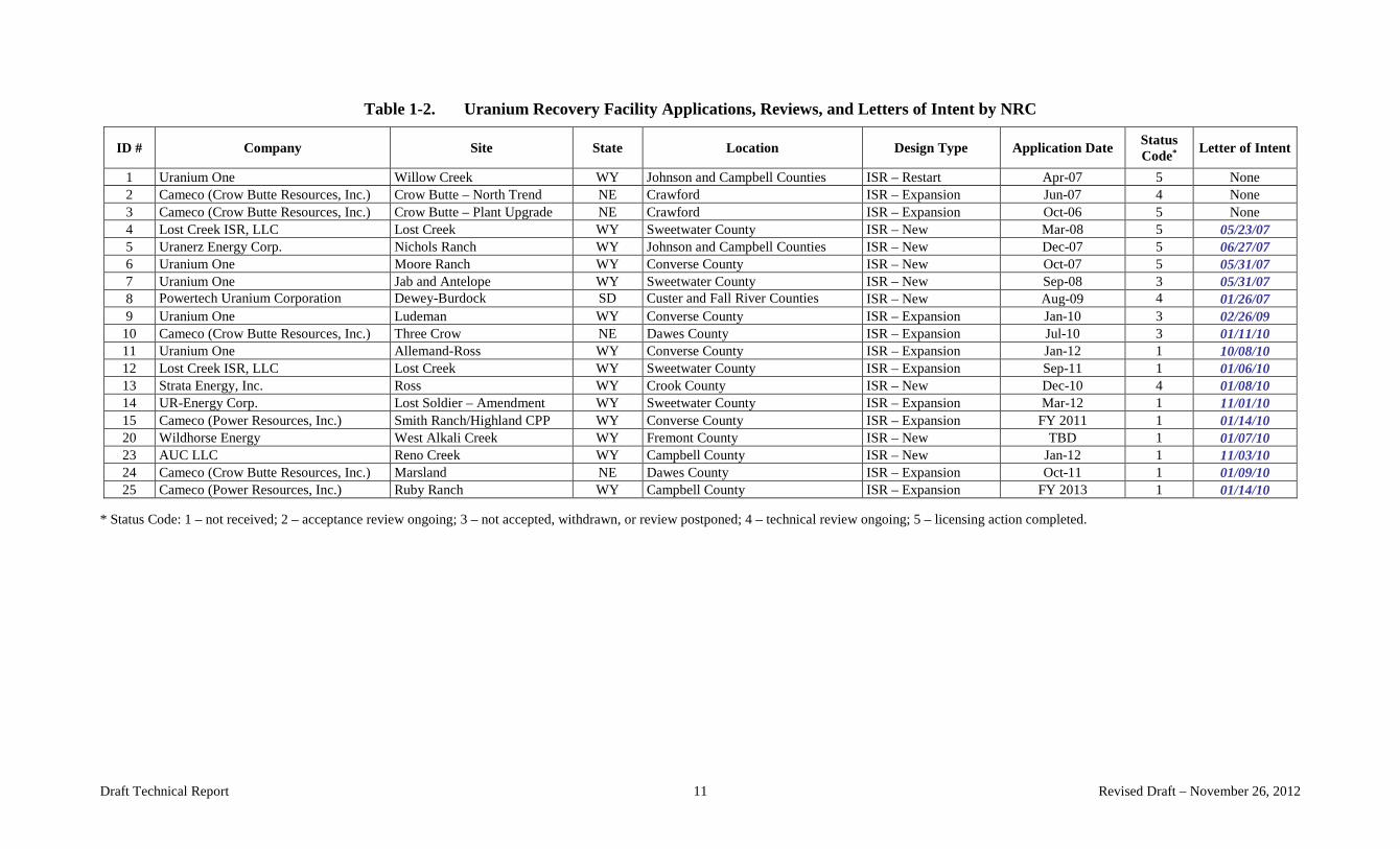
Table 1-2. Uranium Recovery Facility Applications, Reviews, and Letters of Intent by NRC
Status ID # Company Site State Location Design Type Application Date Letter of Intent Code* 1 Uranium One Willow Creek WY Johnson and Campbell Counties ISR – Restart Apr-07 5 None 2 Cameco (Crow Butte Resources, Inc.) Crow Butte – North Trend NE Crawford ISR – Expansion Jun-07 4 None 3 Cameco (Crow Butte Resources, Inc.) Crow Butte – Plant Upgrade NE Crawford ISR – Expansion Oct-06 5 None 4 Lost Creek ISR, LLC Lost Creek WY Sweetwater County ISR – New Mar-08 5 05/23/07 5 Uranerz Energy Corp. Nichols Ranch WY Johnson and Campbell Counties ISR – New Dec-07 5 06/27/07 6 Uranium One Moore Ranch WY Converse County ISR – New Oct-07 5 05/31/07 7 Uranium One Jab and Antelope WY Sweetwater County ISR – New Sep-08 3 05/31/07 8 Powertech Uranium Corporation Dewey-Burdock SD Custer and Fall River Counties ISR – New Aug-09 4 01/26/07 9 Uranium One Ludeman WY Converse County ISR – Expansion Jan-10 3 02/26/09
10 Cameco (Crow Butte Resources, Inc.) Three Crow NE Dawes County ISR – Expansion Jul-10 3 01/11/10 11 Uranium One Allemand-Ross WY Converse County ISR – Expansion Jan-12 1 10/08/10 12 Lost Creek ISR, LLC Lost Creek WY Sweetwater County ISR – Expansion Sep-11 1 01/06/10 13 Strata Energy, Inc. Ross WY Crook County ISR – New Dec-10 4 01/08/10 14 UR-Energy Corp. Lost Soldier – Amendment WY Sweetwater County ISR – Expansion Mar-12 1 11/01/10 15 Cameco (Power Resources, Inc.) Smith Ranch/Highland CPP WY Converse County ISR – Expansion FY 2011 1 01/14/10 20 Wildhorse Energy West Alkali Creek WY Fremont County ISR – New TBD 1 01/07/10 23 AUC LLC Reno Creek WY Campbell County ISR – New Jan-12 1 11/03/10 24 Cameco (Crow Butte Resources, Inc.) Marsland NE Dawes County ISR – Expansion Oct-11 1 01/09/10 25 Cameco (Power Resources, Inc.) Ruby Ranch WY Campbell County ISR – Expansion FY 2013 1 01/14/10
* Status Code: 1 – not received; 2 – acceptance review ongoing; 3 – not accepted, withdrawn, or review postponed; 4 – technical review ongoing; 5 – licensing action completed.
Draft Technical Report 11 Revised Draft – November 26, 2012

The Texas Commission on Environmental Quality (TCEQ) list of Texas ISR sites is presented in Table 1-3 (http://www.uraniuminfo.org/tceq-list-active-and-pending-permits). This list shows that there were four active sites, two proposed sites, two sites undergoing closure, and 30 shutdown sites in Texas as of October 2011.3 Additional background on ISR performance is included in Groundwater Modeling Studies at In Situ Leaching Facilities and Evaluation of Doses and Risks to Off-Site Receptors from Contaminated Groundwater, Revision 1 (SC&A 2011). That report, revised in May 2012, evaluates the risk to down gradient receptors who obtain their water from a contaminated well. Risks are assessed for both radioactive and hazardous chemicals.
3 List provided by Maryann Ryan, Radioactive Materials Division, Texas Commission on Environmental Quality, October 19, 2011.
Draft Technical Report 12 Revised Draft – November 26, 2012
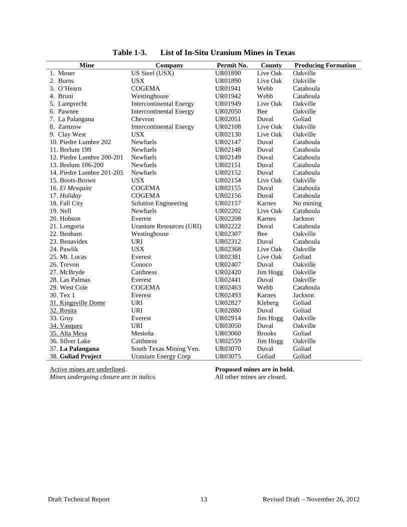
Table 1-3. List of In-Situ Uranium Mines in Texas Mine Company Permit No. County Producing Formation
1. Moser 2. Burns 3. O’Hearn 4. Bruni 5. Lamprecht 6. Pawnee 7. La Palangana 8. Zamzow 9. Clay West 10. Piedre Lumbre 202 11. Brelum 199 12. Piedre Lumbre 200-201 13. Brelum 106-200 14. Piedre Lumbre 201-205 15. Boots-Brown 16. El Mesquite 17. Holiday 18. Fall City 19. Nell 20. Hobson 21. Longoria 22. Benham 23. Benavides 24. Pawlik 25. Mt. Lucas 26. Trevon 27. McBryde 28. Las Palmas 29. West Cole 30. Tex 1 31. Kingsville Dome 32. Rosita
US Steel (USX) USX COGEMA Westinghouse Intercontinental Energy Intercontinental Energy Chevron Intercontinental Energy USX Newfuels Newfuels Newfuels Newfuels Newfuels USX COGEMA COGEMA Solution Engineering Newfuels Everest Uranium Resources (URI) Westinghouse URI USX Everest Conoco Caithness Everest COGEMA Everest URI URI
UR01890 UR01890 UR01941 UR01942 UR01949 UR02050 UR02051 UR02108 UR02130 UR02147 UR02148 UR02149 UR02151 UR02152 UR02154 UR02155 UR02156 UR02157 UR02202 UR02208 UR02222 UR02307 UR02312 UR02368 UR02381 UR02407 UR02420 UR02441 UR02463 UR02493 UR02827 UR02880
Live Oak Live Oak Webb Webb Live Oak Bee Duval Live Oak Live Oak Duval Duval Duval Duval Duval Live Oak Duval Duval Karnes Live Oak Karnes Duval Bee Duval Live Oak Live Oak Duval Jim Hogg Duval Webb Karnes Kleberg Duval
Oakville Oakville Catahoula Catahoula Oakville Oakville Goliad Oakville Oakville Catahoula Catahoula Catahoula Catahoula Catahoula Oakville Catahoula Catahoula No mining Catahoula Jackson Catahoula Oakville Catahoula Oakville Goliad Oakville Oakville Oakville Catahoula Jackson Goliad Goliad
33. Gruy 34. Vasquez 35. Alta Mesa 36. Silver Lake 37. La Palangana 38. Goliad Project
Everest URI Mesteña
UR02914 UR03050 UR03060
Jim Hogg Duval Brooks
Oakville Oakville Goliad
Caithness South Texas Mining Ven. Uranium Energy Corp
UR02559 UR03070 UR03075
Jim Hogg Duval Goliad
Oakville Goliad Goliad
Active mines are underlined. Mines undergoing closure are in italics.
Proposed mines are in bold. All other mines are closed.
Draft Technical Report 13 Revised Draft – November 26, 2012

2.0 RESOURCE CONSERVATION AND RECOVERY ACT This section provides an overview of the RCRA program. Provisions specifically relevant to ISR facility licensing and oversight are discussed in detail. These provisions include Subtitle C facilities, ground water monitoring requirements, and treatment, storage, and disposal facilities (TSDFs). These descriptions of the RCRA program supply context for the development of provisions of the Part 192 revision rulemaking. We are required to be “consistent” with RCRA requirements “to the maximum extent practicable.” Some of the specifics in the ISR revision to Part 192 are derived directly from RCRA program requirements, as noted in later discussions of these requirements. More specifically, the requirements applied to RCRA subtitle C facilities are most appropriate to the ISR operations. 2.1 Summary RCRA was passed in 1976, as an amendment to the Solid Waste Disposal Act of 1965, to ensure that solid wastes are managed in an environmentally sound manner. RCRA gives EPA the authority to control hazardous waste from “cradle-to-grave.” This includes the generation, transportation, treatment, storage, and disposal of hazardous waste (Subtitle C). RCRA also establishes a framework for the management of nonhazardous solid wastes (Subtitle D). Further amendments to RCRA have extended its application; for example, the 1986 amendments to RCRA enabled EPA to address environmental problems that could result from underground tanks storing petroleum and other hazardous substances. RCRA is a key component of EPA’s UMTRCA standards in 40 CFR Part 192. As noted in Chapter 1, Congress specified that EPA’s standards should address nonradiological, as well as radiological, constituents. Therefore, for Title I sites, UMTRCA states that the standards shall, “... to the maximum extent practicable, be consistent with the requirements of the Solid Waste Disposal Act, as amended,” now known as RCRA. For Title II and future NRC-licensed sites, the standards shall be “... consistent with the standards required under subtitle C of the Solid Waste Disposal Act, as amended, which are applicable to such hazards” [UMTRCA section 206(a)]. EPA’s current standards in 40 CFR Part 192 incorporate the RCRA ground water monitoring requirements for hazardous waste units specified in 40 CFR Part 264, including statistical techniques for determining when standards have been achieved. A key question in revising the current rule is whether, and to what extent, it is appropriate to apply these techniques, which were developed to address releases to ground water from engineered hazardous waste units, such as landfills, impoundments, and tanks, to ISR uranium recovery facilities, where the regulated “unit” is a defined portion of an aquifer under 40 CFR Part 146 (see Section 2.3). The RCRA approach to protecting ground water represents a reasonable starting point for developing criteria and standards specific to ISR facilities. The remainder of this chapter provides additional detail on the RCRA requirements and discusses technical challenges in applying those requirements to ISR facilities. It should be emphasized that this chapter describes current RCRA regulations and how they are integrated with 40 CFR 192. It does not explore changes which EPA may adopt as they revise 40 CFR 192. Such changes are discussed in
Draft Technical Report 14 Revised Draft – November 26, 2012

Section 2.3 below and in various sections of the document that discuss the technical issues involved in provisions of the ISR rulemaking. 2.2 Ground Water Monitoring Requirements for Treatment, Storage, and Disposal
Facilities 2.2.1 Overview The ground water monitoring requirements for hazardous waste TSDFs are an important aspect of the RCRA hazardous waste management strategy for protecting human health and the environment from accidental releases of hazardous constituents. While land disposal restrictions and unit-specific standards seek to reduce the toxicity of waste and prevent releases, respectively, the ground water monitoring requirements represent the last line of defense by ensuring that any releases are detected and remediated in a timely manner. TSDFs that manage hazardous waste in landfills, surface impoundments, land treatment units, and some waste piles (referred to as “regulated units” in RCRA) are required to implement a ground water monitoring program to detect the release of hazardous constituents to the underlying ground water. The regulations for permitted facilities are found at 40 CFR Part 264. Specifically, Subpart F addresses releases from solid waste management units and includes elements of a monitoring program such as:
• Ground water protection standard • Hazardous constituents • Concentration limits • Point of compliance • Compliance period • General monitoring requirements • Detection monitoring • Compliance monitoring • Corrective action
The overall goal of these requirements is to protect the ground water in the uppermost aquifer (i.e., the aquifer closest to the TSDF) from contamination by the hazardous constituents managed at the TSDF. 2.2.2 Permitted Facilities For permitted TSDFs, a ground water monitoring program consists of three phases: detection monitoring (§264.98), compliance monitoring (§264.99), and corrective action (§264.100). The phases are sequential, with a facility able to move back and forth between phases as certain criteria are met. The regulations are written as performance standards that require each facility’s ground water monitoring program to have a sufficient number of wells installed at the appropriate locations and depths that can yield representative samples of background conditions and water quality at the point of compliance in the uppermost aquifer (defined as the geological
Draft Technical Report 15 Revised Draft – November 26, 2012
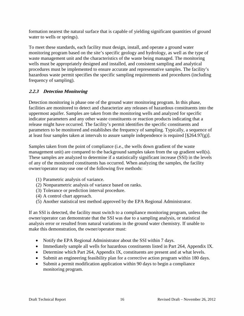
formation nearest the natural surface that is capable of yielding significant quantities of ground water to wells or springs).
To meet these standards, each facility must design, install, and operate a ground water monitoring program based on the site’s specific geology and hydrology, as well as the type of waste management unit and the characteristics of the waste being managed. The monitoring wells must be appropriately designed and installed, and consistent sampling and analytical procedures must be implemented to ensure accurate and representative samples. The facility’s hazardous waste permit specifies the specific sampling requirements and procedures (including frequency of sampling). 2.2.3 Detection Monitoring Detection monitoring is phase one of the ground water monitoring program. In this phase, facilities are monitored to detect and characterize any releases of hazardous constituents into the uppermost aquifer. Samples are taken from the monitoring wells and analyzed for specific indicator parameters and any other waste constituents or reaction products indicating that a release might have occurred. The facility’s permit identifies the specific constituents and parameters to be monitored and establishes the frequency of sampling. Typically, a sequence of at least four samples taken at intervals to assure sample independence is required [§264.97(g)]. Samples taken from the point of compliance (i.e., the wells down gradient of the waste management unit) are compared to the background samples taken from the up gradient well(s). These samples are analyzed to determine if a statistically significant increase (SSI) in the levels of any of the monitored constituents has occurred. When analyzing the samples, the facility owner/operator may use one of the following five methods:
(1) Parametric analysis of variance. (2) Nonparametric analysis of variance based on ranks. (3) Tolerance or prediction interval procedure. (4) A control chart approach. (5) Another statistical test method approved by the EPA Regional Administrator.
If an SSI is detected, the facility must switch to a compliance monitoring program, unless the owner/operator can demonstrate that the SSI was due to a sampling analysis, or statistical analysis error or resulted from natural variations in the ground water chemistry. If unable to make this demonstration, the owner/operator must:
• Notify the EPA Regional Administrator about the SSI within 7 days. • Immediately sample all wells for hazardous constituents listed in Part 264, Appendix IX. • Determine which Part 264, Appendix IX, constituents are present and at what levels. • Submit an engineering feasibility plan for a corrective action program within 180 days. • Submit a permit modification application within 90 days to begin a compliance
monitoring program.
Draft Technical Report 16 Revised Draft – November 26, 2012

2.2.4 Compliance Monitoring The purpose of a compliance monitoring program is to ascertain whether the constituents released to the uppermost aquifer are exceeding acceptable concentration levels and threatening human health and the environment. The first step in this process is establishing a ground water protection standard (GWPS). As stated above, a facility must submit a permit modification application to switch from detection monitoring to compliance monitoring when an SSI is detected. As part of this modified permit, the EPA Regional Administrator specifies the GWPS for the facility. The GWPS establishes:
• The list of hazardous constituents for which to monitor (from Part 261, Appendix VIII).4
• The concentration limits for each of the listed constituents based either on background levels, Safe Drinking Water Act (SDWA) maximum contaminant levels (MCLs), or alternate concentration levels determined by the EPA Regional Administrator.
• The point of compliance, which is the vertical surface at which the facility must monitor the uppermost aquifer to determine if the GWPS is being exceeded.
• The compliance period during which the GWPS applies and compliance monitoring must be continued.
During compliance monitoring, samples are taken at each well located at the point of compliance (four samples from each well) and compared to the GWPS. The EPA Regional Administrator determines the frequency of sampling, which is specified in the modified facility permit. At a minimum, samples must be taken at least semiannually. The facility must also analyze samples for 40 CFR Part 264, Appendix IX, constituents at least annually. If any new constituents are found to have an SSI, then they must be added to the GWPS list of constituents. If the level of any of the constituents exceeds the GWPS, the owner/operator must notify the EPA Regional Administrator in writing within 7 days. The owner/operator also must submit a permit modification application to establish a corrective action program. Compliance monitoring must continue during this period. 2.2.5 Corrective Action Once an exceedance of the GWPS has been detected, the facility must act to bring the constituent concentration levels back into compliance with the GWPS. To achieve this, the owner/operator must either remove the hazardous constituents or treat them in place. The EPA Regional Administrator will approve the facility’s selected corrective action method and specify the time frame in which it must take place. Any hazardous constituents that have migrated beyond the point of compliance also must be remediated. The facility must continue corrective action until the GWPS has not been exceeded for 3 consecutive years. At that point, the facility may return to compliance monitoring.
4 A detailed discussion of hazardous constituents that require monitoring is included in Section 3.5,
“Selection of Parameters to Be Used in Groundwater Sampling Programs.”
Draft Technical Report 17 Revised Draft – November 26, 2012
2.3 Application to ISR Facilities While the application of the RCRA ground water monitoring requirements to conventional mills and tailings impoundments is relatively straightforward, the ISR technology presents additional technical challenges for post-operational monitoring. First, the technology is applied within the aquifer by intentionally altering its chemical characteristics to facilitate transport of uranium. Thus, in the RCRA framework, contaminants have already been released into the environment and are no longer contained within the engineered hazardous waste unit (e.g., a surface impoundment). One perspective on the transference of RCRA approaches to ISR operations is to consider the mined aquifer production wellfield as the “operational unit,” with post-mining restoration activities considered as “engineering” the unit to prevent migration of contaminants beyond its boundaries. Post-restoration monitoring of a “restored” aquifer is then the equivalent of post-closure monitoring around an engineered RCRA disposal facility to assure that contaminants do not escape from the unit and enter the surrounding environment. The intent of the operator to release the site for unrestricted use presents the more significant challenge. Unlike conventional tailings impoundments, which are subject to long-term stewardship requirements, ISR facilities will leave no significant surface facilities or waste behind. The ground water will therefore need to be restored throughout the wellfield, which may show significant heterogeneity. Furthermore, from a corrective action standpoint, the “source” of contamination cannot necessarily be identified as a specific location within the affected area (the ore zone). It is therefore particularly important that an appropriate monitoring program be developed, including an adequate number of wells in the right locations, to determine, with sufficient confidence, that restoration and long-term stability have been achieved. As discussed in this document, there may be technical approaches that can be used to modify or extend the RCRA requirements. Additionally, there may be technical approaches better suited for these particular types of facilities. In a further complication for operating ISR facilities, permits for lixiviant injection wells must be obtained from EPA’s Underground Injection Control (UIC) Program developed pursuant to the SDWA (in some cases, authority to issue UIC permits has been delegated to states). To obtain the required permit, an operating company submits an application to EPA or a Delegated State requesting that an aquifer or portion of an aquifer be exempted from protections of the SDWA. In issuing the UIC permit, the regulatory authority makes a determination whether to grant the exemption and the extent of exemption in the aquifer affected by the activity (40 CFR Part 146). The regulatory authority (EPA 40 CFR Part 144) also permits the drilling of the injection wells. However, it is the NRC or its Agreement States which permit the drilling of production wells, conversion of injection wells to production wells, and also granting the license for the overall uranium extraction project to proceed. The primary concern of the UIC regulatory program is that contaminants not be transported beyond the exempted portion of the aquifer (“excursion”) into an underground source of drinking water (USDW). Requirements for restoration of the exempted portion of the aquifer under the UIC Program are limited compared to the requirements of 40 CFR Part 192. Failure to recognize the applicability of 40 CFR Part 192 to all ground water at an ISR facility (i.e., in the wellfield) has led to a situation in which operators at
Draft Technical Report 18 Revised Draft – November 26, 2012

some ISR facilities have not been held to the more stringent standards in 40 CFR Part 192 (see case studies included in this document). Furthermore, in some cases, the appropriate baseline conditions may not have been recorded. The sections which follow describe the current state of the ISR process and generally how it has been overseen by the NRC or its Agreement States. These regulatory authorities were given the responsibility for uranium extraction oversight under UMTRCA and, in the absence of specific EPA regulatory requirements for ISR facilities, have developed their own procedures and terminology to comply with the overarching EPA regulations for uranium milling in 40 CFR Part 192. In some cases, such as for establishing ACLs, the EPA and NRC regulations were not strictly followed, and no ACL has been established by the NRC to date, even though that agency has allowed restorations above background or MCLs based on considerations such as class of use of the water (e.g., is the restored water acceptable for the same uses as the pre-mining water?).
Draft Technical Report 19 Revised Draft – November 26, 2012

3.0 GROUND WATER MONITORING AT ISR FACILITIES 3.1 Overview The life cycle of an ISR facility typically includes the following ground water-related activities:
• Exploration and development to establish that a commercially viable operation is possible.
• Establishment of site baseline conditions for ISR (mining) of the ore body.
• Recovery of uranium from the ore body.
• Restoration of the ground water to predetermined conditions.
• Demonstration that restored ground water has reached steady state.
• Post-restoration stability monitoring of the ground water.
• Decommissioning of mined area and surface facilities. This report is primarily concerned with the pre- and post-operational aspects of ground water monitoring, specifically establishment of the ground water baseline, demonstration that the restored ground water has reached steady state, and confirmation through post-restoration stability monitoring that the ground water quality is not deteriorating over time after restoration. Figure 3-1 is a graphic representing the evolution of a ground water component of interest during the phases described below. EPA’s 40 CFR Part 192 requires ground water restoration to background (baseline) or to maximum concentration limits (whichever is higher), and in some cases allows the regulator to establish an ACL after meeting 19 rigorous listed criteria. However, NRC has been utilizing a somewhat different standard, termed a “Restoration Goal,” for restoring hazardous constituents in ground water; this standard has not necessarily been compliant with the EPA regulatory standards. Figure 3-1 shows that the measured post-restoration ground water concentration is below the Restoration Goal. In practice, this targeted result may not be realized. This report documents numerous examples where the wellfield was not returned to baseline conditions. In those examples, the regulatory authorities may have determined that the deviations from baseline did not impose serious threats to ground water use ouside the mined area. However, the intention of the 40 CFR 192 rulemaking is to impose a more systematic and consistent regulatory process compatible with other regulatory regimes aimed at protecting ground water. The five phases of ground water monitoring during the life of the ISR facility are:
• Phase 1 – Measure baseline ground water concentrations and establish regulatory approved restoration goals based on statistical procedures that embrace pre-mining temporal and spatial variability.
• Phase 2 – Conduct in-situ mining. Detect lixiviant excursions outside the mining area if they occur. Determine the ground water chemistry at the end of ISR operations.
• Phase 3 – Conduct wellfield restoration. Monitor the progress of restoration through ground water sampling.
Draft Technical Report 20 Revised Draft – November 26, 2012
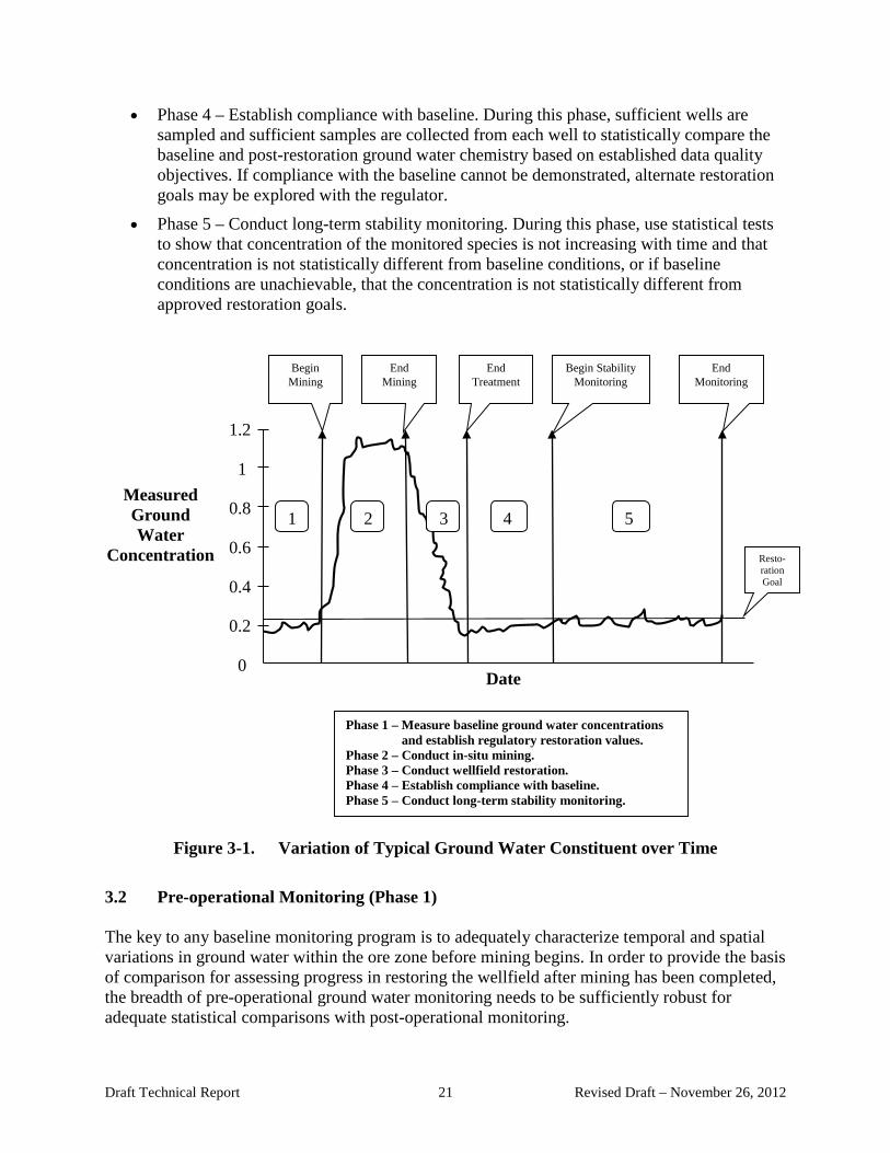
• Phase 4 – Establish compliance with baseline. During this phase, sufficient wells are sampled and sufficient samples are collected from each well to statistically compare the baseline and post-restoration ground water chemistry based on established data quality objectives. If compliance with the baseline cannot be demonstrated, alternate restoration goals may be explored with the regulator.
• Phase 5 – Conduct long-term stability monitoring. During this phase, use statistical tests to show that concentration of the monitored species is not increasing with time and that concentration is not statistically different from baseline conditions, or if baseline conditions are unachievable, that the concentration is not statistically different from approved restoration goals.
Figure 3-1. Variation of Typical Ground Water Constituent over Time
Begin Mining
End Mining
End Treatment
Begin Stability Monitoring
End Monitoring
Resto-ration Goal
1 2 3 4 5
1.2
1
0.8
0.6
0.4
0.2
0 Date
Measured Ground Water
Concentration
Phase 1 – Measure baseline ground water concentrations and establish regulatory restoration values. Phase 2 – Conduct in-situ mining. Phase 3 – Conduct wellfield restoration. Phase 4 – Establish compliance with baseline. P
hase 5 – Conduct long-term stability monitoring.
3.2 Pre-operational Monitoring (Phase 1) The key to any baseline monitoring program is to adequately characterize temporal and spatial variations in ground water within the ore zone before mining begins. In order to provide the basis of comparison for assessing progress in restoring the wellfield after mining has been completed, the breadth of pre-operational ground water monitoring needs to be sufficiently robust for adequate statistical comparisons with post-operational monitoring.
Draft Technical Report 21 Revised Draft – November 26, 2012

3.3 The ISR Leaching Process (Phase 2) During typical ISR operations, chemicals such as sodium carbonate/bicarbonate and gaseous oxygen/hydrogen peroxide are added to the ground water to produce a concentrated oxygen-rich leaching solution called the lixiviant. The lixiviant is injected into the production zone to create ground water oxidizing conditions, which mobilize the uranium from the uranium-rich geologic zone. This mobilized uranium is pumped back to the surface for extraction at a processing plant (Figure 3-2).
Figure 3-2. Idealized Schematic Cross Section to Illustrate Ore-Zone Geology and Lixiviant Migration from an Injection Well to a Production Well (NRC 2009)
The most common injection/pumping patterns are five- and seven-spot (NRC 2003). The shape of the mineralized ore body and surface topography, however, may give rise to other patterns (NRC 1997). A typical five-spot pattern contains four injection wells and one centrally located recovery well. The dimensions of the pattern vary depending on the mineralized zone, but the injection wells are generally between 40 to 150 feet apart. To effectively recover the uranium and also to complete the ground water restoration, the wells are often completed so that they can be used as either injection or recovery wells. During mining operations, a slightly greater volume of water will be recovered from the mineralized zone aquifer than was injected, in order to create a cone of depression or a flow gradient towards the recovery wells. This practice is intended to minimize excursions of leachate outside the production area. Ground water monitoring is necessary to detect any excursions of lixiviant outside the mining area during operations. Figure 3-3 shows typical well arrangements using five- and seven-spot patterns. Figure 3-4 illustrates a
Draft Technical Report 22 Revised Draft – November 26, 2012
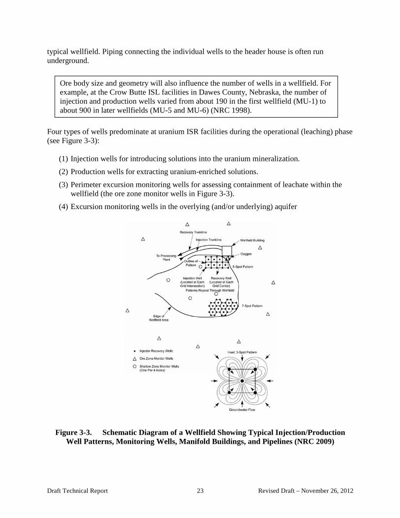
typical wellfield. Piping connecting the individual wells to the header house is often run underground.
Ore body size and geometry will also influence the number of wells in a wellfield. For example, at the Crow Butte ISL facilities in Dawes County, Nebraska, the number of injection and production wells varied from about 190 in the first wellfield (MU-1) to about 900 in later wellfields (MU-5 and MU-6) (NRC 1998).
Four types of wells predominate at uranium ISR facilities during the operational (leaching) phase (see Figure 3-3):
(1) Injection wells for introducing solutions into the uranium mineralization.
(2) Production wells for extracting uranium-enriched solutions.
(3) Perimeter excursion monitoring wells for assessing containment of leachate within the wellfield (the ore zone monitor wells in Figure 3-3).
(4) Excursion monitoring wells in the overlying (and/or underlying) aquifer
Figure 3-3. Schematic Diagram of a Wellfield Showing Typical Injection/Production
Well Patterns, Monitoring Wells, Manifold Buildings, and Pipelines (NRC 2009)
Draft Technical Report 23 Revised Draft – November 26, 2012
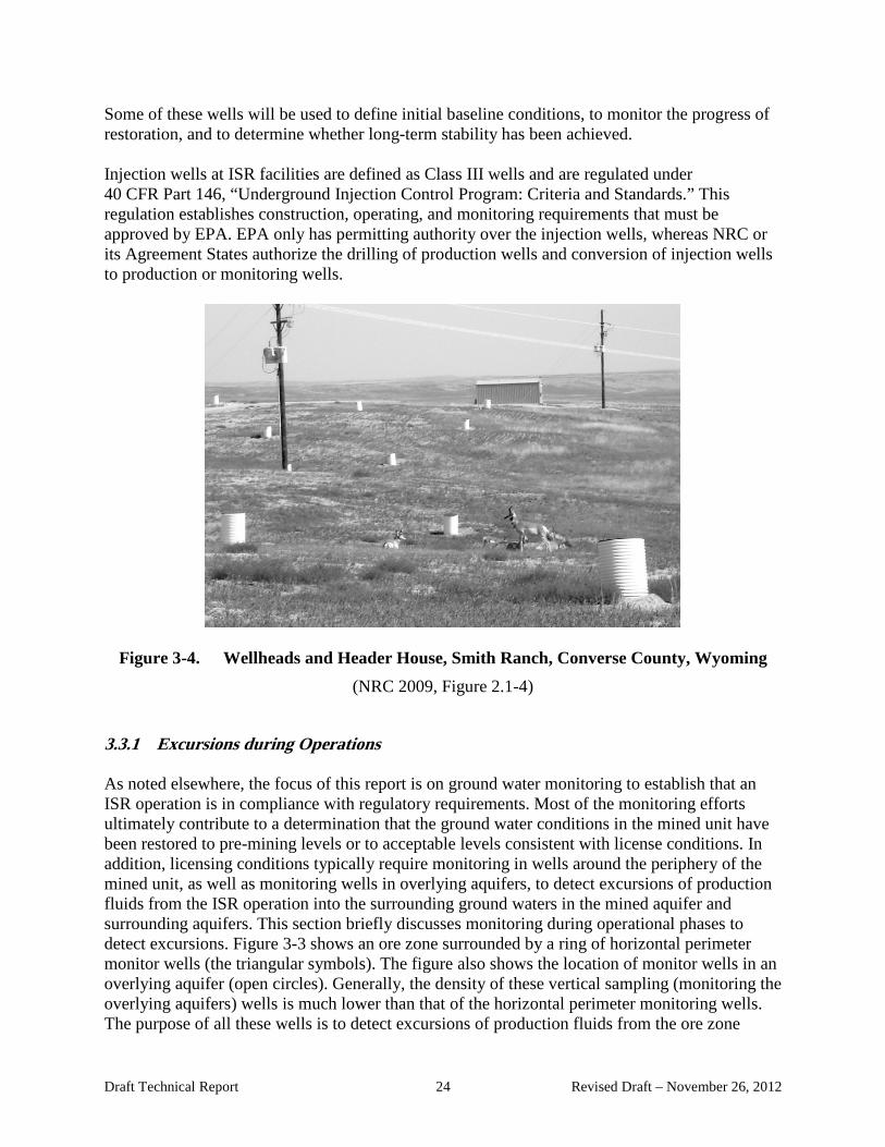
Some of these wells will be used to define initial baseline conditions, to monitor the progress of restoration, and to determine whether long-term stability has been achieved. Injection wells at ISR facilities are defined as Class III wells and are regulated under 40 CFR Part 146, “Underground Injection Control Program: Criteria and Standards.” This regulation establishes construction, operating, and monitoring requirements that must be approved by EPA. EPA only has permitting authority over the injection wells, whereas NRC or its Agreement States authorize the drilling of production wells and conversion of injection wells to production or monitoring wells.
Figure 3-4. Wellheads and Header House, Smith Ranch, Converse County, Wyoming (NRC 2009, Figure 2.1-4)
3.3.1 Excursions during Operations As noted elsewhere, the focus of this report is on ground water monitoring to establish that an ISR operation is in compliance with regulatory requirements. Most of the monitoring efforts ultimately contribute to a determination that the ground water conditions in the mined unit have been restored to pre-mining levels or to acceptable levels consistent with license conditions. In addition, licensing conditions typically require monitoring in wells around the periphery of the mined unit, as well as monitoring wells in overlying aquifers, to detect excursions of production fluids from the ISR operation into the surrounding ground waters in the mined aquifer and surrounding aquifers. This section briefly discusses monitoring during operational phases to detect excursions. Figure 3-3 shows an ore zone surrounded by a ring of horizontal perimeter monitor wells (the triangular symbols). The figure also shows the location of monitor wells in an overlying aquifer (open circles). Generally, the density of these vertical sampling (monitoring the overlying aquifers) wells is much lower than that of the horizontal perimeter monitoring wells. The purpose of all these wells is to detect excursions of production fluids from the ore zone
Draft Technical Report 24 Revised Draft – November 26, 2012

during and after leaching operations. The spacing of horizontal excursion monitoring wells (i.e., wells within the production aquifer) is based on site-specific conditions, but typically they are about 300–500 feet apart. The distances between monitoring wells and the distances of monitoring wells from the wellfield are generally similar. The specific location and spacing of the monitoring wells is established on a site-by-site basis by license condition. The spacing is often modified according to site-specific hydrogeologic characteristics, such as the extent of the confining layer, hydraulic gradient, and aquifer transmissivity (NRC 2009). To fully understand the capabilities of perimeter monitor wells in detecting excursions, their locations relative to the wellfield should be supported with ground water transport modeling. As described in the Wellfield Restoration Report Christensen Ranch Project Wyoming (COGEMA 2008a, Section 8.2.2.1):
Groundwater velocities were calculated for each of the MUs based on hydraulic conductivity, natural hydraulic gradient and porosity estimates. Travel times were calculated for the time to reach the monitor ring (typically 400 feet from the wellfield edge) ... The MU RDPs [restoration data packages] present the data used in the calculations. The range of groundwater velocity determined from those calculations was from 0.0088 to 0.043 ft/d (3.2 to15.5 ft/yr). Estimated travel times to reach the 400 foot monitor well ring ranged from 26 to 123 years.
SC&A has made similar ground water flow simulations at many generic sites (SC&A 2011).5 The SC&A calculations show similar travel times under comparable hydraulic conditions to those presented by COGEMA. Thus, excursions associated with normal advective flow would not be detected over the lifetime of ISR facilities with comparable hydraulic properties.
NRC requires that three species be specified as excursion indicators (e.g., chloride, conductivity, and alkalinity) (see also Section 3.5.5) and deems that an excursion occurs when two of the indicators exceed their established upper control limits (NRC 2003). As described in NRC’s Standard Review Plan (NRC 2003, p. 5-41):
Upper control limits for a specific excursion indicator should be determined on a statistical basis to account for likely spatial and temporal concentration variations within the mineralized zone. Statistical techniques, such as the student’s t-test, are acceptable for setting upper control limits. In some cases, the use of a simple percentage increase above baseline values is acceptable. The staff has decided that in areas with good water quality (a total dissolved solids less than 500 mg/L), setting the upper control limit at a value of 5 standard deviations above the mean of the measured concentrations is an acceptable approach. However, in some aquifers of good water quality, low chloride concentrations have been found to have such a narrow statistical distribution that a specified concentration (e.g., 15 mg/L) above the mean or the mean plus 5 standard deviations approach, which ever is greater, has been used to establish the chloride upper control limit.
5 Revision 2 of this report was issued on May 8, 2012.
Draft Technical Report 25 Revised Draft – November 26, 2012
In practice, establishment of upper control limits may differ from the guidance provided in the Standard Review Plan. For example, in the 2011 draft license renewal at Crow Butte (Crow Butte 2011), the operator is required to collect four samples from each perimeter monitoring well, with at least 14 days between sampling, to establish a baseline for that well. The upper control limits (UCLs) for each of the three indicator parameters are then set equal to the maximum baseline value plus 20%. For parameters with baseline concentrations that average 50 milligrams per liter (mg/L) or less, the operator can chose the maximum baseline plus 20%, the baseline average plus 5 standard deviations, or the baseline average plus 15 mg/L. This is only one approach that has been used at ISR sites. In an earlier operation at Christensen Mine Unit 6 (COGEMA 1996), the UCLs were based on the average of all perimeter wells plus 5 standard deviations. For the chloride excursion indicator, the NRC license allowed use of either the mean plus 5 standard deviations or the mean plus 15 mg/L, whichever was higher. This option was based on the fact that the mean chloride concentration was about 5 mg/L with a standard deviation of less than 1 mg/L. Consequently, use of too tight a UCL could result in false positive indications of lixiviant excursions. Excursions at operational ISR sites are common. Staub et al. (1986) summarized information on excursions at eight sites (seven in Wyoming and one in Texas) developing during the early years of in-situ leaching. Because this study was done early in the use of ISR, several of the sites were experimental rather than full-scale production operations. The authors noted that:
Despite inconsistencies in identifying excursions it is evident that many excursions did occur. Most horizontal excursions were brought under control quickly. However, wells used to monitor for vertical excursions were on excursion status repeatedly and for excessively long periods of time. In many cases restoration procedures were eventually required. It is particularly important to recognize vertical excursions at an early stage in order to avoid costly and time consuming restoration.
The relative intractability of vertical excursions emphasizes the importance of determining that all abandoned boreholes in the area are investigated to ensure that they are properly sealed and that adequate testing is done to fully characterize the local hydrogeology, particularly continuity of the aquitards. Testing the integrity of the production wells against leakage into overlying (or underlying) aquifers is also a concern, since remediation of excursions into these aquifers can be difficult. This also speaks to the importance of having a sufficient number of monitoring wells in the overlying aquifers, so that excursions can be detected early and corrective action taken to avoid the need for extensive restoration activities. 3.3.1.1 Case Histories The examples of actual excursions provided here are not intended to be a comprehensive list of all excursions that have been documented, but rather to provide examples of site-specific excursions and show the periods over which they persist and how they are addressed.
Draft Technical Report 26 Revised Draft – November 26, 2012
Crow Butte The Crow Butte compliance log shows that as of June 2008, about 20 excursions had been reported since mid-1999 (Cohen 2008).
For example, during regularly scheduled biweekly testing of monitor wells at Crow Butte, an excursion in perimeter monitor well CM8-21 was detected when two of the three required indicators (alkalinity and chloride) exceeded the respective UCLs (Teahon 2006a). If a single indicator parameter exceeds the UCL, then a somewhat higher control limit is allowed (the single indicator control limit or SCL, than if two or more indicators exceed the multiple indicator control limit.6 As required by the facility’s NRC license, Crow Butte staff resampled the well within 48 hours and found that the UCLs were still exceeded. Again, as required by NRC license, Crow Butte instituted weekly sampling and unspecified corrective action. Weekly sampling continued from January 24 through April 4, 2006. Samples taken from February 28 through April 4 were below the UCLs, and the well was removed from excursion status. Figure 3-5, Figure 3-6, and Figure 3-7 present charts showing the behavior of the excursion indicators during the excursion of Well CM8-21. Horizontal lines in these figures indicate the control limits: SCL, single indicator control limit, and MCL, multiple indicator control limit. The SCLs are 20% higher than the MCLs. Results for a similar excursion in Crow Butte Well CM9-16 are reported in Teahon 2005a. In another example at Crow Butte, Monitor Well PR-15 was observed to exceed the multiple parameter UCLs for chloride and conductivity on September 6, 2006. This well was a baseline restoration well for Mine Unit 1, which was also being used as a perimeter monitoring well for Mine Unit 2 (Teahon 2006b). The operator noted that restoration activities in Mine Unit 2 adjacent to PR-15 included ground water transfer and wellfield recirculation. Two other baseline restoration wells, IJ-13 and PR-8, from Mine Unit 1, have remained on excursion status since December 27, 2002, and December 23, 2003, respectively. Because of the geometry of Mine Units 2 and 3, the operator believed that PR-15 will continue to exhibit the same trend as IJ-13 and PR-8 until Mine Units 2 and 3 can be fully restored along the perimeter of Mine Unit 1. The increases in chloride and conductivity were associated with a drop in the water level of Well PR-15, presumably a result of ground water transfer. Griffin (2005) discusses problems with shallow monitor Well SM6-28 (i.e., a well in an aquifer overlying the aquifer containing the ore zone). Increases in conductivity and alkalinity were detected in this well on June 16, 2005. Crow Butte Resources (CBR) believed that this apparent excursion was due to increased ground water levels caused by the significant precipitation received at the facility in the spring of 2005 and was not caused by mining activity. This conclusion was supported by the fact that the water level in the well increased 4 feet during the spring and was within 10 feet of the top of the casing at the well. Ground water quality in the area is under the influence of surface water.
6 Exclusively in this section, MCL is the “multiple parameter control limit” and should not be confused with the “maximum contaminant level” used elsewhere in this report.
Draft Technical Report 27 Revised Draft – November 26, 2012
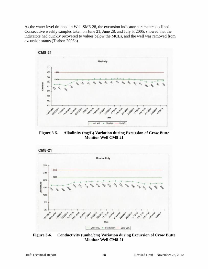
As the water level dropped in Well SM6-28, the excursion indicator parameters declined. Consecutive weekly samples taken on June 21, June 28, and July 5, 2005, showed that the indicators had quickly recovered to values below the MCLs, and the well was removed from excursion status (Teahon 2005b).
Figure 3-5. Alkalinity (mg/L) Variation during Excursion of Crow Butte
Monitor Well CM8-21
Figure 3-6. Conductivity (µmho/cm) Variation during Excursion of Crow Butte
Monitor Well CM8-21
Draft Technical Report 28 Revised Draft – November 26, 2012
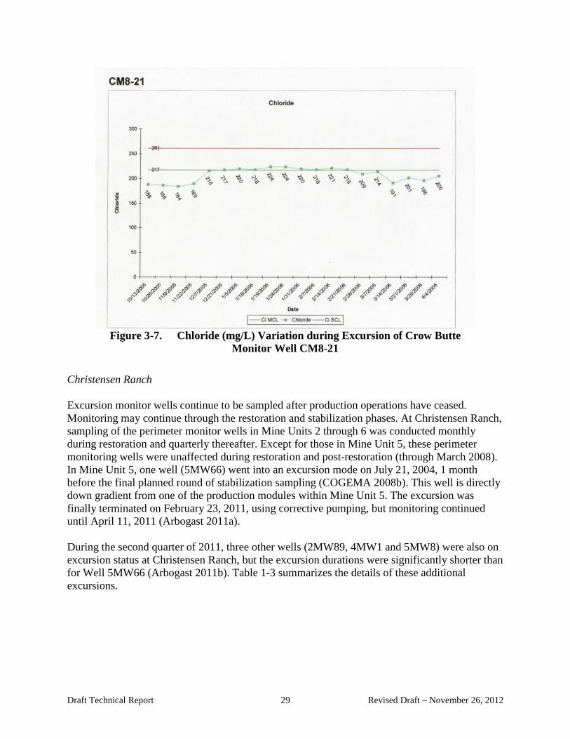
Figure 3-7. Chloride (mg/L) Variation during Excursion of Crow Butte
Monitor Well CM8-21
Christensen Ranch
Excursion monitor wells continue to be sampled after production operations have ceased. Monitoring may continue through the restoration and stabilization phases. At Christensen Ranch, sampling of the perimeter monitor wells in Mine Units 2 through 6 was conducted monthly during restoration and quarterly thereafter. Except for those in Mine Unit 5, these perimeter monitoring wells were unaffected during restoration and post-restoration (through March 2008). In Mine Unit 5, one well (5MW66) went into an excursion mode on July 21, 2004, 1 month before the final planned round of stabilization sampling (COGEMA 2008b). This well is directly down gradient from one of the production modules within Mine Unit 5. The excursion was finally terminated on February 23, 2011, using corrective pumping, but monitoring continued until April 11, 2011 (Arbogast 2011a). During the second quarter of 2011, three other wells (2MW89, 4MW1 and 5MW8) were also on excursion status at Christensen Ranch, but the excursion durations were significantly shorter than for Well 5MW66 (Arbogast 2011b). Table 1-3 summarizes the details of these additional excursions.
Draft Technical Report 29 Revised Draft – November 26, 2012

Table 3-1. Wells on Excursion at Christensen Ranch – 2Q 2011 Well Location On Excursion Off Excursion Corrective Action
2MW89 Perimeter well in March 9, 2011 May 2, 2011 Pumping two restored wellfield of adjacent recovery Mine Unit 2 wells
4MW1 Perimeter well in March 23, 2011 May 16, 2011 Pumping one restored wellfield of adjacent recovery Mine Unit 4 well
5MW8 Perimeter well in April 19, 2011 May 31, 2011 Pumping one restored wellfield of adjacent recovery Mine Unit 5 well
It is noteworthy that these excursions were detected by perimeter monitor wells in restored wellfields for which the operator was seeking restoration approval. Attachment B provides additional details. 3.3.1.2 Summary of Excursion Experience in ISR Operations Excursions of production/restoration waters into monitoring wells within the mined aquifer and overlying aquifers have been observed often and present a problem for the operator and regulator during the period of regulatory control. In most cases, the excursions were quickly restored in the mined unit, which is usually an exempted aquifer, and the excursions appear to pose little long-term potential for contamination to non-exempt ground water down gradient beyond the limits of the exempted area. Excursions into overlying, non-exempt aquifers pose a more significant concern and may require lengthier restoration efforts to remediate the problem, which emphasizes the need for monitoring in the overlying aquifers and measures to test the integrity of the wells against leakage. 3.4 Post-operational Monitoring (Phases 3 through 5)
The intent of restoration efforts is to establish hydrologic and geochemical conditions in the mined areas that will maintain steady-state conditions in all potentially affected aquifers (i.e., overlying, underlying, and adjacent aquifers) and ensure that there is no degradation of water quality from pre-mining conditions. During restoration, the operator monitors progress by periodic sampling and analysis of the ground water constituents to determine when steady-state conditions are attained. Establishing steady-state conditions requires that the ground water potentiometric surface be restored, to the extent practicable, to its preleaching status, so that the flow regime is similar to that existing before mining. In addition, constituents in the ground water must be returned to the predetermined restoration goals and remain at that level for a sufficient period to demonstrate that the results are not trending upwards to higher concentration levels.
Once the operator concludes that restoration is complete and has obtained concurrence from the regulator(s) that a steady state has been established, post-restoration stability monitoring begins. The purpose of the stability monitoring is to demonstrate that the aquifer conditions established at the end of restoration are sustainable over time. Currently, the duration of the stability monitoring period is site specific, with the period established in the license(s). In the past, the license-established post-restoration period typically was about 6 months. More recently, the
Draft Technical Report 30 Revised Draft – November 26, 2012

trend has been to increase the stability monitoring period established in the license. In practice, the actual period of stabilization may be several years, based on iterative analyses of additional samples requested by the regulators.
3.5 Selection of Parameters to Be Used in Ground Water Sampling Programs This section discusses considerations involved in the selection of parameters to be included in ground water monitoring programs at ISR facilities. The focus is on parameters required for baseline and post-restoration compliance monitoring, but parameters required for excursion monitoring and ground water modeling are also included. A site-specific example is provided illustrating how the required monitoring list may be winnowed over time based on field measurements and regulatory approval.
3.5.1 Regulated Constituents 3.5.1.1 EPA Regulations Various EPA regulations establish parameters in the ground water that may require monitoring. Current EPA regulations at 40 CFR Part 192 define constituents to be monitored during processing of uranium ores based on RCRA regulations (see Section 2.0 for a detailed discussion of the RCRA regulations). The standards are presented in §192.32 and are referenced to relevant RCRA regulations there. According to §192.32:
(2) Uranium byproduct materials shall be managed so as to conform to the ground water protection standard in §264.92 of this chapter, except that for the purposes of this subpart:
(i) To the list of hazardous constituents referenced in §264.93 of this chapter are added the chemical elements molybdenum and uranium …
The regulation in §264.93, “Hazardous constituents,” states that:
(a) The Regional Administrator will specify in the facility permit the hazardous constituents to which the ground-water protection standard of §264.92 applies. Hazardous constituents are constituents identified in appendix VIII of part 261 of this chapter that have been detected in ground water in the uppermost aquifer underlying a regulated unit and that are reasonably expected to be in or derived from waste contained in a regulated unit, unless the Regional Administrator has excluded them under paragraph (b) of this section.
The RCRA regulations, in turn, provide in Appendix VIII to 40 CFR Part 261 an extensive list of hazardous constituents for which the EPA Regional Administrator may specify ground water monitoring. Most of the items listed in Appendix VIII are complex organic chemicals such as aldrin; chlordane; lindane; 2,4-D; and DDT. Inorganic species are listed in Table 3-2. The Regional Administrator will include those hazardous constituents from Appendix VIII that have been detected in the ground water. As noted above, EPA added [via §192.32(a)(2)(i)] uranium
Draft Technical Report 31 Revised Draft – November 26, 2012

and molybdenum7 to this list of hazardous constituents. Table 1 of §264.94 defines specific concentration limits for the following hazardous constituents: arsenic, barium, cadmium, chromium, lead, mercury, selenium, silver, and several organic species such as lindane. To the maximum concentration limits in Table 1 of §264.94, EPA added [via §192.32(a)(2)(ii)] combined radium (Ra-226) + Ra-228 and gross alpha (excluding radon and uranium). For those hazardous constituents for which a maximum concentration is not specified, the concentration in the ground water cannot exceed the background level [§264.94(a)(1)]. Additional hazardous constituents from Appendix VIII relevant to ISR facilities for which the background level applies include nickel, molybdenum, thallium, uranium, and vanadium pentoxide (see Table 3-2). The standards in §192.32(a)(2)(iii) also establish a requirement for a monitoring program as specified in §264.98. Section 264.98 references Appendix IX to Part 264 as the source list for hazardous constituents. Appendix IX to Part 264 is similar to Appendix VIII to Part 261 but also includes cobalt, sulfide, tin, vanadium (rather than V2O5), and zinc.
EPA’s National Primary Drinking Water Regulations (NPDWR) specify MCLs for antimony, arsenic, barium, beryllium, cadmium, chromium, copper, fluoride, lead, mercury, nitrate, nitrite, selenium, thallium, gross alpha, beta + gamma, Ra-226 + Ra-228, and uranium (40 CFR Part 141). The MCL is defined as the maximum permissible level of a contaminant in water that is delivered to any user of a public water system. Public water systems have at least 15 service connections or regularly serve an average of at least 25 individuals daily for at least 60 days out of the year. In addition, 40 CFR Part 141 establishes maximum contaminant level goals (MCLGs), which are the maximum levels of a contaminant in drinking water at which no known or anticipated adverse effect on the health of persons would occur, and which allows an adequate margin of safety. MCLGs are nonenforceable health goals.
A Note on Concentration Levels/Limits
According to the NPDWR at §141.2: Maximum contaminant level means the maximum permissible level of a contaminant in water which is delivered to any user of a public water system. Maximum concentration level or limit is not a defined term under RCRA. Rather §264.94 – Concentration Limits refers to the maximum concentration of constituents. Conditions for establishing alternate concentration limits are delineated in §264.94(b).
7 EPA recognized, when it was writing the original uranium milling regulations, the fatal impact of molybdenum on young bovine calves, likely to be present in vicinity of uranium mills or consuming water contaminated from mill effluent.
Draft Technical Report 32 Revised Draft – November 26, 2012
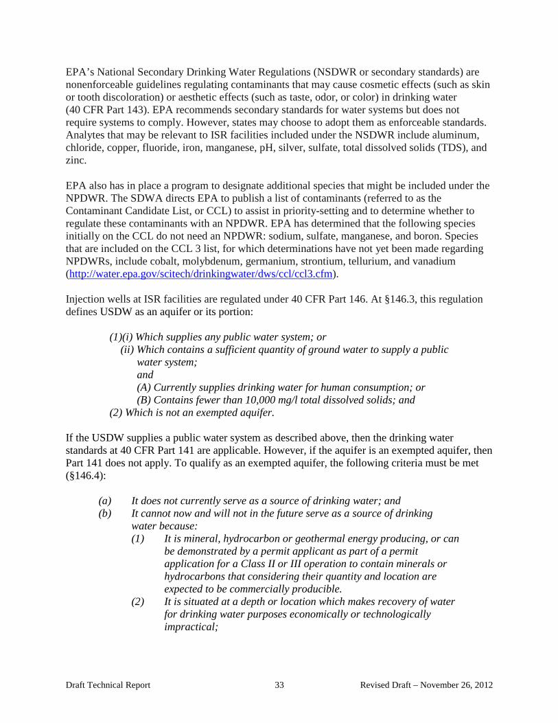
EPA’s National Secondary Drinking Water Regulations (NSDWR or secondary standards) are nonenforceable guidelines regulating contaminants that may cause cosmetic effects (such as skin or tooth discoloration) or aesthetic effects (such as taste, odor, or color) in drinking water (40 CFR Part 143). EPA recommends secondary standards for water systems but does not require systems to comply. However, states may choose to adopt them as enforceable standards. Analytes that may be relevant to ISR facilities included under the NSDWR include aluminum, chloride, copper, fluoride, iron, manganese, pH, silver, sulfate, total dissolved solids (TDS), and zinc.
EPA also has in place a program to designate additional species that might be included under the NPDWR. The SDWA directs EPA to publish a list of contaminants (referred to as the Contaminant Candidate List, or CCL) to assist in priority-setting and to determine whether to regulate these contaminants with an NPDWR. EPA has determined that the following species initially on the CCL do not need an NPDWR: sodium, sulfate, manganese, and boron. Species that are included on the CCL 3 list, for which determinations have not yet been made regarding NPDWRs, include cobalt, molybdenum, germanium, strontium, tellurium, and vanadium (http://water.epa.gov/scitech/drinkingwater/dws/ccl/ccl3.cfm).
Injection wells at ISR facilities are regulated under 40 CFR Part 146. At §146.3, this regulation defines USDW as an aquifer or its portion:
(1)(i) Which supplies any public water system; or (ii) Which contains a sufficient quantity of ground water to supply a public
water system; and (A) Currently supplies drinking water for human consumption; or (B) Contains fewer than 10,000 mg/l total dissolved solids; and (2) Which is not an exempted aquifer.
If the USDW supplies a public water system as described above, then the drinking water standards at 40 CFR Part 141 are applicable. However, if the aquifer is an exempted aquifer, then Part 141 does not apply. To qualify as an exempted aquifer, the following criteria must be met (§146.4):
(a) It does not currently serve as a source of drinking water; and (b) It cannot now and will not in the future serve as a source of drinking
water because: (1) It is mineral, hydrocarbon or geothermal energy producing, or can
be demonstrated by a permit applicant as part of a permit application for a Class II or III operation to contain minerals or hydrocarbons that considering their quantity and location are expected to be commercially producible.
(2) It is situated at a depth or location which makes recovery of water for drinking water purposes economically or technologically impractical;
Draft Technical Report 33 Revised Draft – November 26, 2012
(3) It is so contaminated that it would be economically or technologically impractical to render that water fit for human consumption; or
(4) It is located over a Class III well mining area subject to subsidence or catastrophic collapse; or
(c) The total dissolved solids content of the ground water is more than 3,000 and less than 10,000 mg/l and it is not reasonably expected to supply a public water system.
Table 3-2 summarizes the species that may require monitoring under various EPA regulations described above and indicates limits specified in the regulations. It should be noted that some differences exist between the RCRA regulatory limits in Table 1 of 40 CFR 264.94 and the MCLs in the National Drinking Water Regulations at 40 CFR Part 141. The table also lists nonmandatory MCLGs below which no health effects are expected and the nonmandatory MCLs for NSDWRs at 40 CFR Part 143.
Draft Technical Report 34 Revised Draft – November 26, 2012

Table 3-2. Ground Water Require
Species Identified in EPA Regulations Monitoring at ISR Facilities
That May
Species EPA Regulation Regulatory Concentration Limit (mg/L)
40 CFR 264.94 (Table 1)
40 CFR 141 (MCL)b
40 CFR 141 (MCLG)
40 CFR 143 (MCL)c
Molybdenum §192.32(a)(2)(i) Uranium §192.32(a)(2)(i) /40 CFR 141 0.03 Ra-226 + Ra-228 §192.32(a)(2)(ii) /40 CFR 141 5 (pCi/L) 5 (pCi/L) 0 Gross alpha (ex. U and radon) §192.32(a)(2)(ii) /40 CFR 141 15 (pCi/L) 0
Nickel §264.93/§261, Appendix VIII
Thallium §264.93/§261, Appendix VIII/ 40 CFR 141 0.002 0.0005
Vanadium Pentoxide §264.93/§261, Appendix VIII Arsenic §264.94, Table 1/40 CFR 141 0.05 0.010 0 Barium §264.94, Table 1/40 CFR 141 1.0 2 2 Cadmium §264.94, Table 1/40 CFR 141 0.01 0.005 0.005 Chromium §264.94, Table 1/40 CFR 141 0.05 0.1 0.1 Cobalt §264.98 (Appendix IX) Lead §264.94, Table 1/40 CFR 141 0.05 0.015 0 Mercury §264.94, Table 1/40 CFR 141 0.002 0.002 0.002 Selenium §264.94, Table 1/40 CFR 141 0.01 0.05 Silver §264.94, Table 1/40 CFR 141 0.05 0.1 Sulfide §264.98 (Appendix IX) Tin §264.98 (Appendix IX) Antimony 40 CFR 141 0.006 0.006 Beryllium 40 CFR 141 0.004 Copper 40 CFR 141/40 CFR 143 1.3 1.3 1.0 Fluoride 40 CFR 141/40 CFR 143 4 4 2.0
Nitrate 40 CFR 141 10 (as nitrogen) (as
10 nitrogen)
Nitrite 40 CFR 141 1 (as nitrogen)
1 (as nitrogen)
Total nitrate plus nitrite 40 CFR 141 10 (as nitrogen)
10 (as nitrogen)
Beta + gamma 40 CFR 141 < 4 mrem/yr dose Aluminum 40 CFR 143/CCL 0.05 to 0.2 Chloride 40 CFR 143 4 (MRDL)a 250 Iron 40 CFR 143 0.3 Manganese 40 CFR 143 0.05 pH 40 CFR 143 6.5–8.5 Sulfate 40 CFR 143 250 Total dissolved solids 40 CFR 143 500
Zinc 40 CFR 143/§264.98 (Appendix IX) 5
Vanadium CCL/§264.98 (Appendix IX) a – MRDL (maximum residual disinfectant level) b – mandatory MCL per NPDWR c - non-mandatory MCL per NSDWR
Draft Technical Report 35 Revised Draft – November 26, 2012
3.5.1.2 NRC Requirements
According to NRC’s “Standard Review Plan for In Situ Leach Uranium Extraction License Applications,” Section 2.7.3(4), which describes the acceptance criteria for site characterization hydrology (NRC 2003):
Reasonably comprehensive chemical and radiochemical analyses of water samples, obtained within and at locations away from the mineralized zone(s), have been made to determine pre-operational baseline conditions. Baseline water quality should be determined for the mineralized and surrounding aquifers. These data should include water quality parameters that are expected to increase in concentration as a result of in situ leach activities and that are of concern to the water use of the aquifer (i.e., drinking water, etc.). The applicant should show that water samples were collected by acceptable sampling procedures, such as American Society for Testing and Materials D4448 (American Society for Testing and Materials, 1992).
For example, in situ leach operations are not expected to mobilize aluminum, and unless an ammonia-based lixiviant is used, ammonia concentrations in the ground water should not increase as a result of in situ leach operations. Therefore, little is gained by sampling these parameters. Studies have shown that thorium-230 is mobilized by bicarbonate-laden leaching solutions. However, studies have also shown that after restoration, thorium in the ground water will not remain in solution because the chemistry of thorium causes it to precipitate and chemically react with the rock matrix (Hem, 1970). As a result of its low solubility in natural waters, thorium is found in only trace concentrations. Additionally, chemical tests for thorium are expensive, and are not commonly included in water analyses at in situ leach facilities.
Section 5.7.8.3 of NRC 2003 states:
The applicant should identify the list of constituents sampled for baseline concentrations. Table 2.7.3-1 [see Column 3, Table 3-3 of this report] provides a list of acceptable constituents for monitoring at in situ leach facilities. Alternatively, applicants may propose a list of constituents that is tailored to a particular location. In such cases, sufficient technical bases must be provided to demonstrate the acceptability of the selected constituent list.
3.5.1.3 State of Texas Requirements
TCEQ provides guidance8 on ground water analyses. This guidance specifies measurement of the 26 parameters listed in the following table:
8 Texas Administrative Code, Title 30, Part 1, Chapter 331, Subchapter F, Rule §331.104.
Draft Technical Report 36 Revised Draft – November 26, 2012
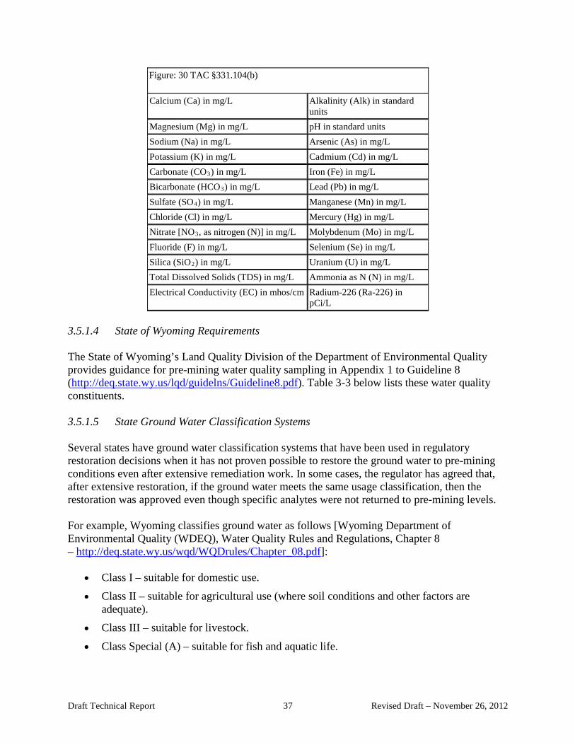
Figure: 30 TAC §331.104(b)
Calcium (Ca) in mg/L Alkalinity (Alk) in standard units
Magnesium (Mg) in mg/L pH in standard units Sodium (Na) in mg/L Arsenic (As) in mg/L Potassium (K) in mg/L Cadmium (Cd) in mg/L Carbonate (CO3) in mg/L Iron (Fe) in mg/L Bicarbonate (HCO3) in mg/L Lead (Pb) in mg/L Sulfate (SO4) in mg/L Manganese (Mn) in mg/L Chloride (Cl) in mg/L Mercury (Hg) in mg/L Nitrate [NO3, as nitrogen (N)] in mg/L Molybdenum (Mo) in mg/L Fluoride (F) in mg/L Selenium (Se) in mg/L Silica (SiO2) in mg/L Uranium (U) in mg/L Total Dissolved Solids (TDS) in mg/L Ammonia as N (N) in mg/L Electrical Conductivity (EC) in mhos/cm Radium-226 (Ra-226) in
pCi/L 3.5.1.4 State of Wyoming Requirements The State of Wyoming’s Land Quality Division of the Department of Environmental Quality provides guidance for pre-mining water quality sampling in Appendix 1 to Guideline 8 (http://deq.state.wy.us/lqd/guidelns/Guideline8.pdf). Table 3-3 below lists these water quality constituents. 3.5.1.5 State Ground Water Classification Systems Several states have ground water classification systems that have been used in regulatory restoration decisions when it has not proven possible to restore the ground water to pre-mining conditions even after extensive remediation work. In some cases, the regulator has agreed that, after extensive restoration, if the ground water meets the same usage classification, then the restoration was approved even though specific analytes were not returned to pre-mining levels. For example, Wyoming classifies ground water as follows [Wyoming Department of Environmental Quality (WDEQ), Water Quality Rules and Regulations, Chapter 8 – http://deq.state.wy.us/wqd/WQDrules/Chapter_08.pdf]:
• Class I – suitable for domestic use.
• Class II – suitable for agricultural use (where soil conditions and other factors are adequate).
• Class III – suitable for livestock.
• Class Special (A) – suitable for fish and aquatic life.
Draft Technical Report 37 Revised Draft – November 26, 2012
• Class IV – suitable for industry (Class IV(A) – TDS ≤ 10,000 mg/L; Class IV (B) – TDS >10,000 mg/L).
• Class V – associated with commercial deposits of hydrocarbons and/or other minerals or considered a geothermal resource.
Table I of Chapter 8 of the WDEQ regulations specifies allowable concentrations for Class I, II, and III constituents. In the case of ISR facilities, the water would likely be Class V. According to the regulations, any discharge into the Class V ground water “shall not result in degradation or pollution of the associated or other ground water and, at a minimum, shall be returned to a condition and quality consistent with the pre-discharge use suitability of the water.”
South Dakota water quality regulations specify that ground water containing 10,000 mg/L or less of TDS is “classified as having the beneficial use of drinking water supplies, suitable for human consumption” (South Dakota Administrative Rules 74:54:01:03 – http://legis.state.sd.us/rules/DisplayRule.aspx?Rule=74:54:01:03). It is not clear how the state addresses ground water with concentrations above 10,000 mg/L.
In Texas, under the Texas Risk Reduction Program rule, all ground water-bearing units affected by, or reasonably anticipated to be affected by, chemicals of concern having concentrations at or above residential ground water assessment levels must be characterized with regard to the applicable ground water resource classification (TCEQ 2010). A “ground water-bearing unit” is defined as a saturated geologic formation, group of formations, or part of a formation that has a hydraulic conductivity equal to or greater than 1 × 10⁻⁵ centimeters per second (cm/sec). The Texas Risk Reduction Program establishes three categories of ground water resources, designated Classes 1, 2, and 3, based on a site-specific evaluation of the current use of the ground water-bearing unit, as well as its potential use, as defined on the basis of natural water quality and well yield. Only saturated geologic units with hydraulic conductivities of K ≥1 × 10⁻⁵ cm/sec meet the definition of a ground water-bearing unit.
The ground water class establishes the types of response measures that may be employed (decontamination/removal versus control) and the ground water protective concentration level (PCL). For Class 1 ground water resources, affected ground water must be removed and/or decontaminated to the critical PCL; control options are not permitted. For affected Class 2 or Class 3 ground water resources, affected ground water must be removed and/or decontaminated to the critical PCL, unless a plume management zone is approved, or such remediation is demonstrated to be technically impracticable, in which case a plume management zone is required. A key factor in establishing the ground water class is the TDS:
• Class 1 – < 1,000 mg/L or ≤ 3,000 mg/L and meets 40 CFR Part 141 NPDWR standards.
• Class 2 – ≤ 10,000 mg/L.
• Class 3 – > 10,000 mg/L.
The PCLs for Class 3 water are 100 times the PCLs for Classes 1 and 2.
Draft Technical Report 38 Revised Draft – November 26, 2012
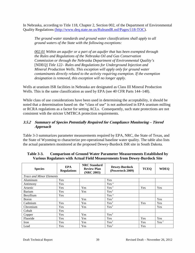
In Nebraska, according to Title 118, Chapter 2, Section 002, of the Department of Environmental Quality Regulations (http://www.deq.state.ne.us/RuleandR.nsf/Pages/118-TOC).
The ground water standards and ground water classifications shall apply to all ground waters of the State with the following exceptions:
002.01 Within an aquifer or a part of an aquifer that has been exempted through the Rules and Regulations of the Nebraska Oil and Gas Conservation Commission or through the Nebraska Department of Environmental Quality’s [NDEQ] Title 122– Rules and Regulations for Underground Injection and Mineral Production Wells. This exception will apply only for ground water contaminants directly related to the activity requiring exemption. If the exemption designation is removed, this exception will no longer apply.
Wells at uranium ISR facilities in Nebraska are designated as Class III Mineral Production Wells. This is the same classification as used by EPA (see 40 CFR Parts 144–148).
While class of use considerations have been used in determining the acceptability, it should be noted that a determination based on the “class of use” is not authorized in EPA uranium milling or RCRA regulations as a factor for setting ACLs. Consequently, such state protections are not consistent with the stricter UMTRCA protection requirements.
3.5.2 Summary of Species Potentially Required for Compliance Monitoring – Tiered Approach
Table 3-3 summarizes parameter measurements required by EPA, NRC, the State of Texas, and the State of Wyoming to characterize pre-operational baseline water quality. The table also lists the actual parameters monitored at the proposed Dewey-Burdock ISR site in South Dakota.
Table 3-3. Comparison of Ground Water Parameter Measurements Established by Various Regulators with Actual Field Measurements from Dewey-Burdock Site
Species EPA Regulations
NRC Standard Review Plan (NRC 2003)
Dewey-Burdock (Powertech 2009) TCEQ WDEQ
Trace and Minor Elements Aluminum Yes Yes Antimony Yes Yes e Arsenic Yes Yes Yes f Yes Yes Barium Yes Yes Yes f Beryllium Yes Yes e Boron Yes Yes f Yes Cadmium Yes Yes Yes f Yes Yes Chromium Yes Yes Yes f Yes Cobalt Yes Copper Yes Yes Yes f Fluoride Yes Yes Yes Yes Yes Iron Yes Yes Yes f Yes Yes f Lead Yes Yes Yes f Yes
Draft Technical Report 39 Revised Draft – November 26, 2012

Table 3-3. Comparison of Ground Water Parameter Measurements Established by Various Regulators with Actual Field Measurements from Dewey-Burdock Site
Species EPA Regulations
NRC Standard Review Plan (NRC 2003)
Dewey-Burdock (Powertech 2009) TCEQ WDEQ
Manganese Yes Yes Yes f Yes Yes Mercury Yes Yes Yes f Yes Molybdenum Yes Yes Yes f Yes Yes Nickel Yes Yes Yes f Selenium Yes Yes Yes inc. SeIV & SeVI f Yes Yes Silver Yes Yes Yes f Strontium Yes e Thallium Yes Yes e Tin Yes Uranium Yes Yes Yes f Yes Yes Vanadium Yes &V2O5 Yes Yes Yes Zinc Yes Yes Yes f Yes Common Constituents Alkalinity Yes Yes Ammonia Yes Yes Yes Bicarbonate Yes Yes Yes Yes Calcium Yes Yes Yes Yes Carbonate Yes Yes Yes Yes Chloride Yes Yes Yes Yes Yes Magnesium Yes Yes Yes Yes Nitrate Yes Yes Yes Yes Yes Nitrite Yes Yes Yes Potassium Yes Yes Yes Yes Silica Yes Yes Sodium Yes Yes Yes Yes Sulfate Yes Yes Yes Yes Yes Sulfide Yes Chemical and Physical Indicators Anion/Cation Balance Yes Sodium Adsorption Potential
Yes
Specific Conductivity Yes a Yes Yes pH Yes Yes a Yes Yes Redox Potential Yes Total Dissolved Solids Yes Yesb Yes Yes Yes Radiological Parameters Gross Alpha Yes Yes c Yes Yes Gross Beta Yes Yes Yes Gross Gamma Yes Lead-210 g Polonium-210 Yes g Radium-226 Yes + Ra-228 Yes d Yes g Yes Yes Radon-222 Yes Radium-228 See note d Yes Thorium-230 Yes g Thorium-232 Yes Beta + Gamma Yes
Draft Technical Report 40 Revised Draft – November 26, 2012

Table 3-3. Comparison of Ground Water Parameter Measurements Established by Various Regulators with Actual Field Measurements from Dewey-Burdock Site
Species EPA Regulations
NRC Standard Review Plan (NRC 2003)
Dewey-Burdock (Powertech 2009) TCEQ WDEQ
a – field and laboratory determination; b – laboratory only; c – excluding radon, radium, and uranium; d – if site initial sampling indicates the presence of Th-232, then Ra-228 should be considered in the baseline sampling or an alternative may be proposed; e – total; f – dissolved and total; g – dissolved, suspended, and total.
Hazardous constituents listed by EPA but not included in the NRC Standard Review Plan include aluminum, antimony, beryllium, thallium, gross alpha, and beta plus gamma. However, as shown in Column 4 of Table 3-3 for the proposed Dewey-Burdock site (which is undergoing technical review by NRC), all of the hazardous constituents listed by EPA are included in the ground water sampling protocols. In fact, the pre-operational sampling conducted by the Powertech Uranium Corporation includes several species not listed by either EPA or NRC. Several of these additional consitutents were added by the State of South Dakota. Attachment A provides additional details on the Dewey-Burdock background sampling program.
The NRC Standard Review Plan includes boron, which EPA has determined not to be a hazardous constituent, as noted above.
The sampling requirements of the TCEQ are more limited with respect to hazardous constituents than those included in EPA regulations. Hazardous constituents not listed by TCEQ include barium, beryllium, chromium, copper, nickel, silver, thallium, and vanadium.
In addition to hazardous constituents drawn from EPA regulations, a variety of other species must be measured to assess chemical and geochemical reactions occurring during in situ leaching and to provide early warning of potential wellfield excursions. Since the lixiviant used in the leaching process is typically carbonate/bicarbonate solution enhanced with an oxidant (e.g., oxygen or hydrogen peroxide), these species are typically included in ground water sampling programs. Nonsorbing tracers that provide early warning of excursions from the wellfield during operations are also sampled. As discussed below, these may include chloride, total alkalinity, and conductivity. Since the mobilization of uranium involves oxidation-reduction reactions, monitoring of constituents that provide indications of the redox state of the ground water may also be required. These may include redox potential, iron (Fe+2/Fe+3), selenium (Se+4/Se+6), As(III)/As(V), and S-2/SO4-2.
The U.S. Geological Survey (USGS) has suggested that dissolved oxygen should also be monitored to better understand redox reactions occurring in the ground water (NRC 2007, p. 23). To date, regulators have not included dissolved oxygen in the required suite of constituents to be monitored in ground water.
The suite of constituents to be analyzed may vary over the life of a wellfield. A full suite of samples including all the species listed by EPA and the additional species listed by NRC in its Standard Review Plan (NRC 2003), shown above in Table 3-3, Columns 2 and 3, would provide the basis for a sample suite to be used for establishing the wellfield baseline, Phase 1 in Figure
Draft Technical Report 41 Revised Draft – November 26, 2012

3-1. Some of the listed constituents may not be detected in the baseline ground water. However, since there is a possibility that nondetectable concentrations of specific constituents could become measurable because of the introduction of the lixiviant and geochemical changes within the aquifer during mining, the same suite of samples should be used to characterize the ground water at the end of mining (Phase 2 of Figure 3-1). If some of the sampled constituents are not detected in Phase 1 or Phase 2, then consideration should be given to eliminating those constituents from monitoring during Phases 3, 4, and 5 as defined in Figure 3-1. In addition, it may be appropriate to eliminate other constituents from Phases 3, 4, and 5 monitoring if the constituents are not deemed to provide significant incremental information about ground water quality. Species such as sodium, potassium, ammonia (unless it is added to the lixiviant), and SiO2 might fall into this category. However, if geochemical modeling is required, elimination of these species may not be possible since an anion/cation balance will be needed. Temperature and TDS may also be needed to confirm that the thermodynamic database for the geochemical model is valid. The next section discusses these requirements in greater detail.
In summary, the initial list of analytes for monitoring during Phase 1 and Phase 2 would include all of the inorganic species listed in the EPA regulations (Column 2 of Table 3-3), in addition to any species listed in the NRC Standard Review Plan (Column 3 of Table 3-3) that are not on the EPA list. For ground water monitoring during Phases 3–5, the initial list would be reduced by eliminating those species not detected during Phase 1 and Phase 2. The monitoring list for Phases 3–5 could be further condensed by eliminating certain nonhazardous species judged not to significantly impact ground water quality or adversely impact the ability to perform geochemical modeling. Compiling listings of species to be determined for an ISR operation can be regarded as a “tiering” approach in that the contaminants regulated by various regulatory authorities would comprise the top tier in an analytical scheme. These species would include radionuclides and other species with adverse health effects. They would always require measurement. Those species used for other purposes, such as detecting excursions, determining water quality, and geochemical modeling exercises would be the next “tier” in a sampling and analysis plan. Many of these species would also be required to demonstrate compliance with regulatory requirements, although not directly tied to assessing potential adverse health effects. An example would be a species used as an indicator of excursions and as a measure restoration. Species on the lower tier list may be dropped from a sampling and testing protocol at different stages of the ISR operation if they are determined to have no role in controlling radionuclide and toxic metal concentrations and contaminant migration. For any specific ISR operation, the listing of species for measurement should be stated initially in the licenseing process and subject to revision on the basis of data collected during operations (see Section 3.5.6 below for an example).
3.5.3 Well Construction and Low-Flow Sampling Methodologies
The construction of the production, injection or monitoring wells involves sealing the units overlying the production zone with steel, fiberglass or PVC casing that is grouted in place (NRC 2009). A typical well completion is shown in Figure 3-8. Other potential types of well construction are described in NMA (2007).
Draft Technical Report 42 Revised Draft – November 26, 2012
The type of grout, screen and casing materials are selected based upon the chemistry of the lixiviant and ground water, the depth of the target interval and the expected injection pressures. PVC or fiberglass casings are generally used in wells less than 1,000 ft deep, while deeper wells or wells that will be subject to high pressures are generally constructed with steel or fiberglass casing and well screens (NRC 2009). The potential that chemical reactions may take place between the casing material and the dissolved constituents in the ground water also needs to be considered in selecting well construction materials.
As described in Puls and Barcelona (1996) and EPA (2010d), the water in the well casing may not be representative of the aquifer, and therefore needs to be excluded from the ground water samples. Wells are purged to some extent prior to sampling for the following reasons: the presence of the air interface at the top of the water column resulting in an oxygen concentration gradient with depth, leaching from or sorption to the casing or filter pack, chemical changes due to clay seals or backfill, and potential surface water infiltration into the annular space of a poorly constructed or deteriorating well.
Low-flow refers to the velocity with which water enters the pump intake and that is imparted to the formation pore water in the immediate vicinity of the well screen. Water level drawdown within the well provides the best indication of the stress imparted by a given flow-rate for a given hydrological situation. The objective is to pump in a manner that minimizes vertical flow within the borehole, and draws formation water through the well screen to the pump.
Ground water sampling at ISR facilities is typically based on low-flow methods stabilization of the water quality parameters within pre-determined ranges based upon historical data (NRC 2006). Stabilization parameters generally include electrical conductance, pH, oxidation-reduction potential, turbidity, dissolved oxygen and temperature (NRC 2006). Major differences between typical procedures used in low-flow sampling at RCRA and CERCLA sites versus ISR facilities are the pumping rates are generally much higher at ISR facilities (5 to 10 gpm versus 0.1 to 0.25 gpm), the screened intervals are generally greater than 25 feet (versus 10 feet) (NRC 2006), and the well diameters for the ISR wells are much larger (4 to 6 inches versus 2 inches for typical RCRA and CERCLA wells).
Draft Technical Report 43 Revised Draft – November 26, 2012
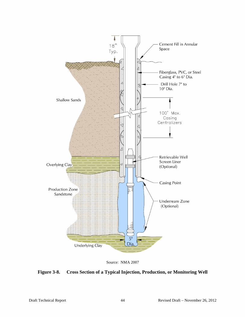
Source: NMA 2007
Figure 3-8. Cross Section of a Typical Injection, Production, or Monitoring Well
Draft Technical Report 44 Revised Draft – November 26, 2012

3.5.4 Species Required for Geochemical Modeling
To adequately comprehend the potential mobility of uranium in ground water, a sufficient degree of site characterization has to be conducted to understand hydrogeologic and geochemical conditions and also the extent and distribution of any contaminant plumes and sources. As discussed in EPA 2002c, sample collection programs are designed around goals associated with specific project objectives. Data quality objectives (DQOs) define the types, quality, and quantity of data required by the various aspects of a project. Once the DQOs are developed, appropriate sampling methodologies, analytical protocols, and specific methods may be considered and selected. For instance, the DQOs may be different if project goals emphasize detection and monitoring of contaminant concentrations rather than geochemical speciation modeling. The types of data required to fulfill the conceptual model needs related to the geochemistry are presented below.
3.5.4.1 Aqueous Chemistry
A simplified conceptualization of the major speciation reactions that geochemical modeling attempts to simulate are shown in Figure 3-9. During active mining, an oxidant (lixiviant) is injected that releases oxygen (O2) in order to solubilize the uranium from the uraninite (upper mineral shown in Figure 3-9) into uranyl carbonate complexes (UO2CO 0
3 ), which are extracted in solution to the surface. The injected oxidant also reacts with pyrite that releases dissolved iron and subsequently precipitates some form of hydrous ferric oxide (HFO). The HFO precipitate that forms is a mixture of iron-bearing minerals that often includes microcrystalline goethite. Uranyl ions derived from the uraninite will also be adsorbed to the surface of the goethite and as uranyl surface complexes (Hfo_wOUO +2
2 ) and removed from solution. This surface complexation reaction could be particularly important in the restoration phase (Gard and Mahoney 2012). Characterization of geochemical conditions within an aquifer requires careful collection of data (e.g., major ions) necessary for input into geochemical models. The sensitivity of uranium to redox conditions also requires that precautions be taken during sampling and analysis to ensure that results obtained are representative of ground water chemistry. The following are considered “core parameters for ground water” for predicting uranium concentrations (EPA 2002c) in ground water:
• Temperature. • Oxidation-reduction potential (corrected to redox), pH, alkalinity. • Turbidity. • Total and ferrous iron. • Dissolved oxygen. • Specific conductance. • Dissolved organic carbon. • Major ions (Ca2+, Mg2+, Na+, K+, Cl-, S2-, SO 2-
4 , NO 2-3 , ammonium, phosphate).
• Aluminum, silica, manganese.
Collection of turbidity data is important for a variety of reasons, including its usefulness as a sampling equilibration parameter using low-flow techniques where metals are contaminants of
Draft Technical Report 45 Revised Draft – November 26, 2012

concern. Turbidity data can also be helpful in explaining data anomalies (e.g., high total iron concentrations under oxidizing conditions) and evaluating the influence of particulates on metals concentrations. The collection of major anion and cation data is important for proper evaluation of the aqueous geochemistry of the system and for performance of accurate geochemical modeling in support of a site conceptual model. Fluoride is important in some hydrogeologic settings because of its high complexing capacity and thus, is needed to determine the adequacy of ion balances for geochemical modeling purposes. Additional information on this topic is covered in EPA 2002c.
Source: Gard and Mahoney 2012
Figure 3-9. Major Chemical Reactions Involved in Uranium Recovery and Restoration
Specification of the appropriate methodology for the collection and analysis of the above listed parameters is beyond the scope of this document; however, descriptions of techniques and methods can be found in EPA 2002c, ASTM procedures (e.g. ASTM 2010), and the USGS online field manuals. Certain parameters must be measured in the field because of stability issues, and others are recommended to be field measurements (EPA 2002c). Parameters that must be measured in the field include temperature, pH, Eh, dissolved oxygen, and turbidity. The use of low-flow sampling is recommended as described in EPA 2010a. Specific conductance and alkalinity are also recommended for field analysis (EPA 2002c). Redox indicators such as Fe(II), S2-, and H2 should be measured in the field rather than in the laboratory; EPA 2002c describes special considerations with respect to their measurements. 3.5.4.2 Solid Phase Geochemistry Solid phase characterization should be included for sites where uranium or other inorganic contaminants in ground water are being evaluated. The solid phase should be tested to confirm the form of the uranium associated with the mineralogy of the solid phase, and to determine its
Draft Technical Report 46 Revised Draft – November 26, 2012
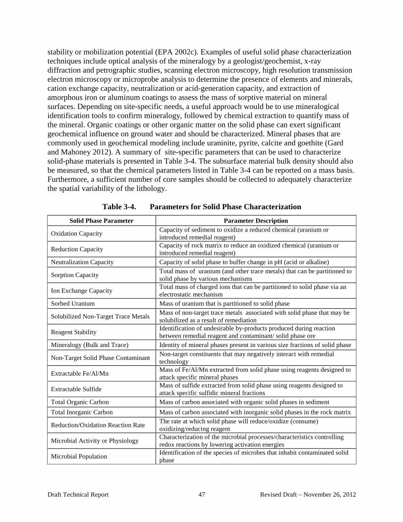
stability or mobilization potential (EPA 2002c). Examples of useful solid phase characterization techniques include optical analysis of the mineralogy by a geologist/geochemist, x-ray diffraction and petrographic studies, scanning electron microscopy, high resolution transmission electron microscopy or microprobe analysis to determine the presence of elements and minerals, cation exchange capacity, neutralization or acid-generation capacity, and extraction of amorphous iron or aluminum coatings to assess the mass of sorptive material on mineral surfaces. Depending on site-specific needs, a useful approach would be to use mineralogical identification tools to confirm mineralogy, followed by chemical extraction to quantify mass of the mineral. Organic coatings or other organic matter on the solid phase can exert significant geochemical influence on ground water and should be characterized. Mineral phases that are commonly used in geochemical modeling include uraninite, pyrite, calcite and goethite (Gard and Mahoney 2012). A summary of site-specific parameters that can be used to characterize solid-phase materials is presented in Table 3-4. The subsurface material bulk density should also be measured, so that the chemical parameters listed in Table 3-4 can be reported on a mass basis. Furthermore, a sufficient number of core samples should be collected to adequately characterize the spatial variability of the lithology.
Table 3-4. Parameters for Solid Phase Characterization
Solid Phase Parameter Parameter Description
Oxidation Capacity Capacity of sediment to oxidize a reduced chemical (uranium or introduced remedial reagent)
Reduction Capacity Capacity of rock matrix to reduce an oxidized chemical (uranium or introduced remedial reagent)
Neutralization Capacity Capacity of solid phase to buffer change in pH (acid or alkaline)
Sorption Capacity Total mass of uranium (and other trace metals) that can be partitioned to solid phase by various mechanisms
Ion Exchange Capacity Total mass of charged ions that can be partitioned to solid phase via an electrostatic mechanism
Sorbed Uranium Mass of uranium that is partitioned to solid phase
Solubilized Non-Target Trace Metals Mass of non-target trace metals associated with solid phase that may be solubilized as a result of remediation
Reagent Stability Identification of undesirable by-products produced during reaction between remedial reagent and contaminant/ solid phase ore
Mineralogy (Bulk and Trace) Identity of mineral phases present in various size fractions of solid phase
Non-Target Solid Phase Contaminant Non-target constituents that may negatively interact with remedial technology
Extractable Fe/Al/Mn Mass of Fe/Al/Mn extracted from solid phase using reagents designed to attack specific mineral phases
Extractable Sulfide Mass of sulfide extracted from solid phase using reagents designed to attack specific sulfidic mineral fractions
Total Organic Carbon Mass of carbon associated with organic solid phases in sediment Total Inorganic Carbon Mass of carbon associated with inorganic solid phases in the rock matrix
Reduction/Oxidation Reaction Rate The rate at which solid phase will reduce/oxidize (consume) oxidizing/reducing reagent
Microbial Activity or Physiology Characterization of the microbial processes/characteristics controlling redox reactions by lowering activation energies
Microbial Population Identification of the species of microbes that inhabit contaminated solid phase
Draft Technical Report 47 Revised Draft – November 26, 2012

Table 3-4. Parameters for Solid Phase Characterization
Solid Phase Parameter Parameter Description
Aquifer Permeability The ability of aquifer material to transmit ground measurement of porosity
water based on
Bulk Density Defined as the mass of many total volume they occupy
particles of the material divided by the
Source: Modified from EPA 2002c
Collection of solid phase samples in the field for later mineralogical analysis also requires careful attention and handling in order to preserve conditions as they are in the aquifer. Minerals that are stable under a reducing environment (such as in an aquifer) will be subject to alteration when exposed to oxygen. Removal of pore water from the sample may also cause some transformations. Significant changes in reactivity may result from changes in mineral structure and surface area due to drying at even slightly elevated temperatures. Careful handling is necessary for proper preservation of solid samples for subsequent characterization. Specification of precise procedures for sampling and handling solid-phase samples is beyond the scope of this report but is discussed in EPA 2002c. If it is necessary, however, that solid-phase characterization be included as part of site investigations where ground water is contaminated with uranium, then additional planning and expense will be involved compared to typical current site characterization practices. For example, recommended procedures for sample cores obtained in the field for mineralogical or other solid phase characterization are that they should be immediately capped and frozen, placed in a cooler or freezer, and later thawed under an oxygen-free or inert atmosphere (EPA 2002c). Procedures will vary depending on site-specific concerns and the analyses being performed. It is reasonable to expect that characterization will be necessary at locations within contaminated and uncontaminated areas of an aquifer with the number of samples related to the degree of heterogeneity.
3.5.5 Species Required for Excursion Monitoring While the focus of this report is on post-restoration monitoring, to ensure completeness of the discussion of constituents requiring monitoring at ISRs, this section briefly discusses excursion monitoring. Monitoring of chemical species that can serve as leading indicators in detecting excursions before the arrival of hazardous constituents is an essential operational feature at ISR facilities. NRC requires use of three such indicators and notes the following (NRC 2003):
The choice of excursion indicators is based on lixiviant content and ground-water geochemistry. Ideal excursion indicators are measurable parameters that are found in significantly higher concentrations during in situ leach operations than in the natural waters. At most uranium in situ leach operations, chloride is an excellent excursion indicator because it acts as a conservative tracer, it is easily measured, and chloride concentrations are significantly increased during in situ leaching. Conductivity, which is correlated to total dissolved solids, is also considered to be a good excursion indicator (Staub[et al.], 1986; Deutsch [et al.], 1985). Total alkalinity (carbonate plus bicarbonate plus hydroxide) is an excellent indicator in well fields where sodium bicarbonate or carbon dioxide is used in the lixiviant. If conductivity is used to estimate total dissolved solids,
Draft Technical Report 48 Revised Draft – November 26, 2012
measurements will be normalized to a reference temperature, usually 25 °C, because of the temperature dependence of conductivity.
Calcium, sodium, and sulfate are usually found at significantly higher levels in in situ solutions than in natural ground-water concentrations. The use of cations (e.g., calcium 2+, sodium+) as excursion indicators is generally not appropriate because they are subject to ion exchange with the host rock. The use of sulfate may give false alarms because of induced oxidation around a monitor well (Staub [et al.], 1986; Deutsch [et al.], 1985)… Although water level changes in artesian aquifers are quickly transmitted, water levels are generally not considered good indicators, because water levels tend to have significant natural variability. The applicant may choose to add a non-reactive, conservative tracer to in situ leach solutions to act as an excursion indicator. The applicant is required to provide the technical bases for the selection of excursion indicators.
3.5.6 Case History – Evolution of Constituent Monitoring List
Experience at the Crow Butte ISR site in Nebraska provides an example of how the list of ground water analytes required to be monitored evolves during operations. The original NRC license (SUA-1534, dated March 4, 1998) specified in Section 10.3B that the following species be analyzed to establish the baseline (and by inference the parameters to be monitored after the cessation of mining): alkalinity, barium, bicarbonate, boron, cadmium, calcium, carbonate, chloride, chromium, copper, fluoride, iron, lead, magnesium, manganese, mercury, molybdenum, nickel, nitrate, nitrite, pH, potassium, Ra-226, selenium, silica, sodium, specific conductivity, sulfate, temperature, total dissolved solids, uranium, vanadium, and zinc. The highlighted items here are parameters that were included in the license agreement but were not listed in the NRC Standard Review Plan (NRC 2003) and shown in Table 3-3, Column 3 above. In addition, silver, gross alpha, and gross beta are listed in the Standard Review Plan but not included in the Crow Butte license. Crow Butte subsequently requested that NRC remove alkalinity, bicarbonate, boron, carbonate, chromium, nitrate, specific conductivity, and temperature from the list of monitored parameters, and NRC granted the request as part of License Amendment 11, dated June 26, 2001 (Leach 2001). Crow Butte’s rationale for the requested changes was as follows:
• Alkalinity, bicarbonate, and carbonate can be evaluated as a single parameter – total carbonate.9
• Boron was a constituent of concern because it could affect crop growth. Although small amounts of boron were detected in pre- and post-mining ground water, there is virtually no use of ground water for irrigation in the area, so boron would not affect surface plants.
Draft Technical Report 49 Revised Draft – November 26, 2012
9 However, as noted above, data on individual species may be required if geochemical modeling is done.

• Post-extraction concentrations of chromium in the ground water were below the limit of detection, thus negating the need for further analyses.
• Specific conductivity is a general indicator of the ionic concentration of the ground water. However, the same information can be derived from measurement of TDS, which is a required parameter.
• Measurements of nitrate showed that baseline and post-mining results were essentially the same and were a factor of two lower than levels which might give rise to concerns about health effects.
• Comparison of baseline and post-mining levels of silica showed that the silica concentrations were essentially the same before and after leaching.
• Crow Butte argued that the uranium recovery process does not affect ground water temperature, and NRC accepted this reasoning.
NRC allowed some constituents to be removed from the required monitoring list because they found that the elements duplicated information provided by other parameters, because they believed that the ISR process had little effect on baseline values, because the quantity present in the ground water was below the limit, or because health effects would be insignificant. All of these determinations were based on site-specific information, regulatory review, and license amendment. EPA did not participate in these determinations.
3.5.7 Formal Approach to Acceptable Restoration
The primary goal of restoration is to return all analytes to the value determined by baseline monitoring. According to NRC practice, this value may be the baseline mean value or some higher value based on the statistical variability of the mean. However, it is well documented throughout this report that restoration of all analytes to baseline conditions is a difficult task, and baseline values may not be re-established for some species even after extensive remediation measures. Addressing the behavior of those analytes that EPA has defined as hazardous should be the focus during restoration (see Table 3-2).
For those analytes with EPA quantitative regulatory limits, as described in Table 3-2, any analyte that is above baseline after restoration but below the prescribed regulatory limit should be acceptable without further action in accordance with EPA requirements. As noted above, this will require reconciliation of certain limits in §264.94 and the MCLs in 40 CFR Parts 141 and 143.
For analytes that exceed the nonmandatory MCLs, as described in 40 CFR Part 143 [Secondary Drinking Water Regulations (SDWRs)], the operator is allowed to demonstrate to the NRC or its Agreement States through geochemical and ground water modeling or other techniques that the measured concentrations do not pose a significant risk to human health or the environment. For example, it might be possible to demonstrate that the ground water transport time to the nearest receptor well is on the order of thousands of years. In the case of high sulfate content, it might be possible to demonstrate through geochemical modeling that the excess sulfate is important in ensuring that radium is removed by precipitation. While iron has a nonmandatory limit of 0.3 mg/L, the existence of high soluble iron (Fe+2) may be indicative of reducing conditions that tend
Draft Technical Report 50 Revised Draft – November 26, 2012
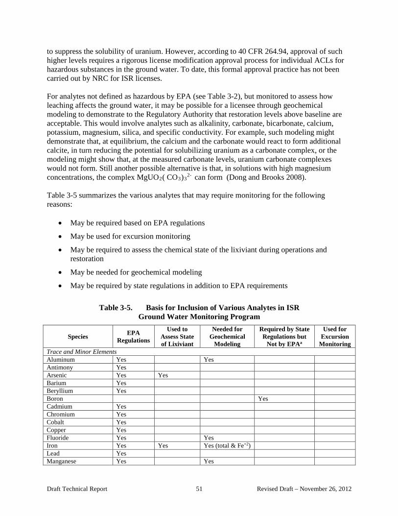
to suppress the solubility of uranium. However, according to 40 CFR 264.94, approval of such higher levels requires a rigorous license modification approval process for individual ACLs for hazardous substances in the ground water. To date, this formal approval practice has not been carried out by NRC for ISR licenses. For analytes not defined as hazardous by EPA (see Table 3-2), but monitored to assess how leaching affects the ground water, it may be possible for a licensee through geochemical modeling to demonstrate to the Regulatory Authority that restoration levels above baseline are acceptable. This would involve analytes such as alkalinity, carbonate, bicarbonate, calcium, potassium, magnesium, silica, and specific conductivity. For example, such modeling might demonstrate that, at equilibrium, the calcium and the carbonate would react to form additional calcite, in turn reducing the potential for solubilizing uranium as a carbonate complex, or the modeling might show that, at the measured carbonate levels, uranium carbonate complexes would not form. Still another possible alternative is that, in solutions with high magnesium concentrations, the complex MgUO 2-
2( CO3)3 can form (Dong and Brooks 2008). Table 3-5 summarizes the various analytes that may require monitoring for the following reasons:
• May be required based on EPA regulations
• May be used for excursion monitoring
• May be required to assess the chemical state of the lixiviant during operations and restoration
• May be needed for geochemical modeling
• May be required by state regulations in addition to EPA requirements
Table 3-5. Basis for Inclusion of Various Analytes in
Ground Water Monitoring Program ISR
Species EPA Regulations
Used to Assess State of Lixiviant
Needed for Geochemical
Modeling
Required by State Regulations but
Not by EPAa
Used for Excursion
Monitoring Trace and Minor Elements Aluminum Yes Yes Antimony Yes Arsenic Yes Yes Barium Yes Beryllium Yes Boron Yes Cadmium Yes Chromium Yes Cobalt Yes Copper Yes Fluoride Yes Yes Iron Yes Yes Yes (total & Fe+2) Lead Yes Manganese Yes Yes
Draft Technical Report 51 Revised Draft – November 26, 2012
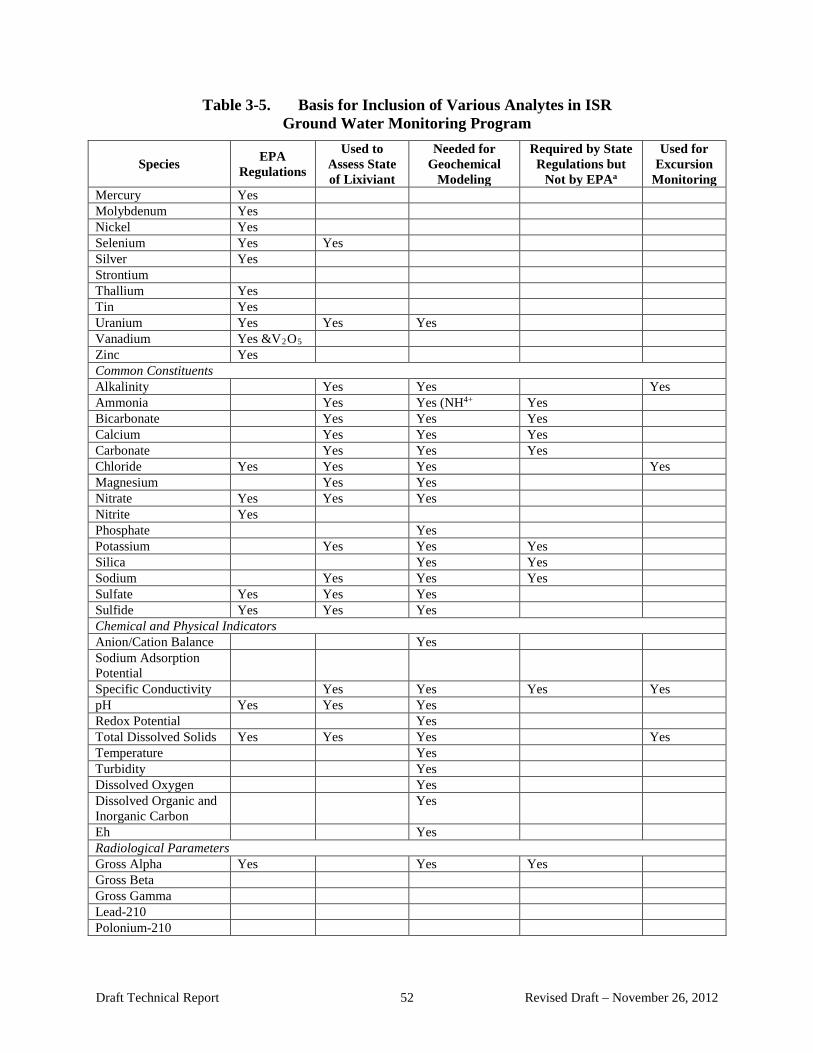
Table 3-5. Basis for Inclusion of Various Analytes in ISR Ground Water Monitoring Program
Species EPA Regulations
Used to Assess State of Lixiviant
Needed for Geochemical
Modeling
Required by State Regulations but
Not by EPAa
Used for Excursion
Monitoring Mercury Yes Molybdenum Yes Nickel Yes Selenium Yes Yes Silver Yes Strontium Thallium Yes Tin Yes Uranium Yes Yes Yes Vanadium Yes &V2O5 Zinc Yes Common Constituents Alkalinity Yes Yes Yes Ammonia Yes Yes (NH4+ Yes Bicarbonate Yes Yes Yes Calcium Yes Yes Yes Carbonate Yes Yes Yes Chloride Yes Yes Yes Yes Magnesium Yes Yes Nitrate Yes Yes Yes Nitrite Yes Phosphate Yes Potassium Yes Yes Yes Silica Yes Yes Sodium Yes Yes Yes Sulfate Yes Yes Yes Sulfide Yes Yes Yes Chemical and Physical Indicators Anion/Cation Balance Yes Sodium Adsorption Potential
Specific Conductivity Yes Yes Yes Yes pH Yes Yes Yes Redox Potential Yes Total Dissolved Solids Yes Yes Yes Yes Temperature Yes Turbidity Yes Dissolved Oxygen Yes Dissolved Organic and Inorganic Carbon
Yes
Eh Yes Radiological Parameters Gross Alpha Yes Yes Yes Gross Beta Gross Gamma Lead-210 Polonium-210
Draft Technical Report 52 Revised Draft – November 26, 2012
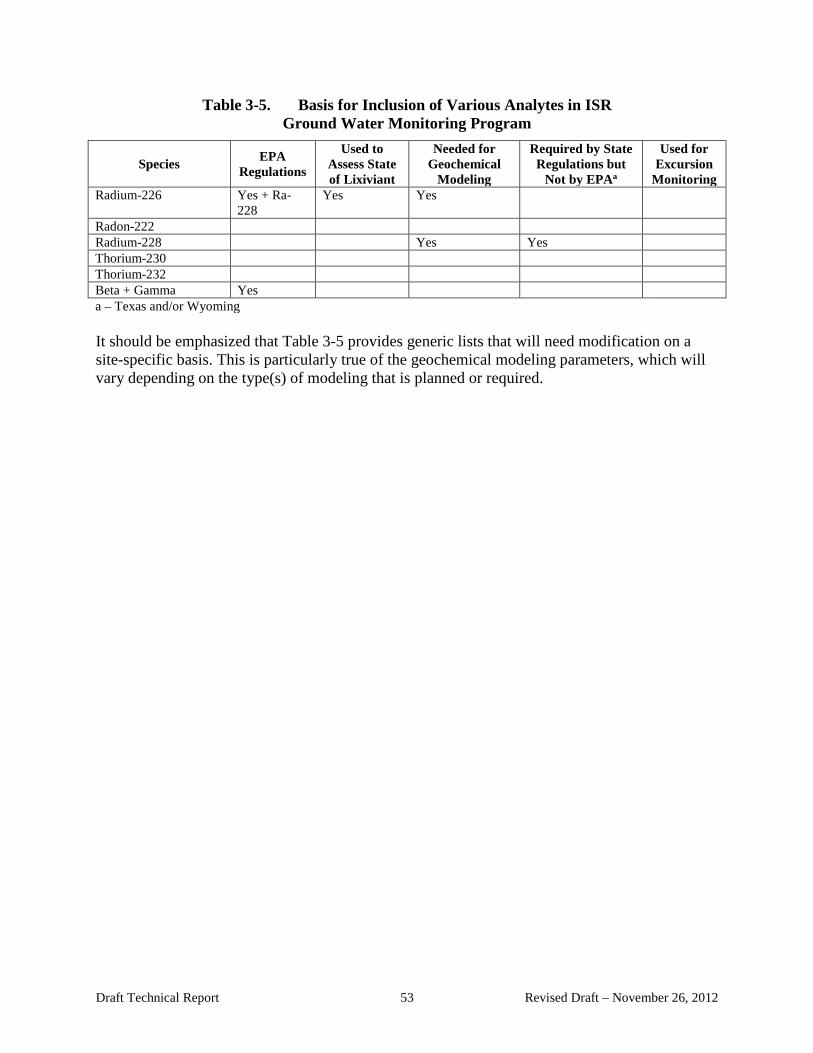
Table 3-5. Basis for Inclusion of Various Analytes in ISR Ground Water Monitoring Program
Species EPA Regulations
Used to Assess State of Lixiviant
Needed for Geochemical
Modeling
Required by State Regulations but
Not by EPAa
Used for Excursion
Monitoring Radium-226 Yes + Ra-
228 Yes Yes
Radon-222 Radium-228 Yes Yes Thorium-230 Thorium-232 Beta + Gamma Yes a – Texas and/or Wyoming It should be emphasized that Table 3-5 provides generic lists that will need modification on a site-specific basis. This is particularly true of the geochemical modeling parameters, which will vary depending on the type(s) of modeling that is planned or required.
Draft Technical Report 53 Revised Draft – November 26, 2012

4.0 TECHNICAL CONSIDERATIONS FOR ISR GROUND WATER MONITORING Monitoring wells within an in-situ mining area and site vicinity serve vital functions necessary for efficient uranium recovery with minimal adverse environmental impacts. Proper monitor well placement and data collection from these wells ensure that the aquifer constituents are detected and then restored to pre-mining levels. Without adequate placement of monitoring wells and proper data collection, which includes consideration of sample frequency and sampling time frame, mine operators and regulators (1) may not detect excursions of lixiviant outside the mining area during operations, and (2) may not be able to confidently determine whether the impacted aquifer needs further restoration or has been restored to its pre-mining state or to predetermined conditions specified by regulators. This section focuses on technical considerations for ground water monitoring through all operational phases of an ISR facility. Because the monitoring goals and practices depend on the characteristics of the ore body, this section begins with a discussion of geographic, geologic, and chemical characteristics typical of uranium deposits suitable for leaching. 4.1 Uranium Geology The geographic areas that are considered to be potential resources of uranium in the United States are shown in Figure 4-1. The principal regions of uranium recovery by ISR are the Wyoming basin, the Colorado Plateau, and the Gulf Coastal Plain of Texas (Figure 4-2). The southern Black Hills in South Dakota and northeast Colorado/western Nebraska within the Great Plains region also contain sedimentary uranium deposits amenable to ISR. Furthermore, exploration is ongoing elsewhere in the U.S. that could expand the extent of production to other states, such as Michigan or Alaska, and to types of uranium deposits (other than roll-front) that could be extracted through ISR methods.
(Source: DOE 1980)
Figure 4-1. Uranium Resource Areas of the United States
Draft Technical Report 54 Revised Draft – November 26, 2012

(Source: NMA 2007)
Figure 4-2. Pending, Licensed, and Active ISL Operations
4.1.1 Formation of Uranium Containing Ore Deposits Based on the shape of the ore body and relationship to the depositional or structural environment, sandstone uranium deposits can be subdivided into three types (these may be gradational into each other): tabular, roll-front, and remnant-primary sandstone (Hou 2004). Tabular and roll-front mineralized bodies form along the contact of sand and intercalated clay horizons and at paleochannel margins (Figure 4-3), while remnant-primary sandstone deposits may occur in sandstones adjacent or vertically stacked along a permeable fault zone (Figure 4-4). Precipitation of uranium minerals in most tabular deposits is thought to begin shortly after sedimentation and burial. Mineral detritus and rock fragments derived from weathered bedrock are deposited, along with channel sediments. The uranium is leached under oxidizing and slightly acidic conditions and is mobilized in ground water moving through the sediments, with mineralization commonly accompanying diagenesis of the sediments.
Draft Technical Report 55 Revised Draft – November 26, 2012
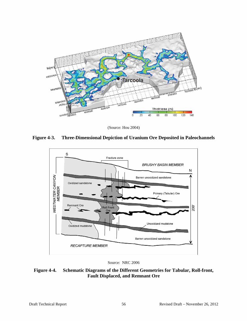
(Source: Hou 2004)
Figure 4-3. Three-Dimensional Depiction of Uranium Ore Deposited in Paleochannels
Source: NRC 2006
Figure 4-4. Schematic Diagrams of the Different Geometries for Tabular, Roll-front, Fault Displaced, and Remnant Ore
Draft Technical Report 56 Revised Draft – November 26, 2012

In Nebraska, New Mexico, Texas and Wyoming, the general geology and formation of roll-front deposits is nearly identical with the host rock being relatively near-surface sandstone that was deposited in fluvial or lacustrian environments (NMA 2007). Aquifers and lithologic units underlying topographically high areas, such as ridges, are recharged by rainfall that has elevated oxygen and carbonic acid, which solubilizes low concentrations of uranium (and other metals) from the soils and rocks. The mobilized uranium moves deeper into the formation into areas where the ground water is being reduced by organic carbon, carbonized fossil wood, pyrite and/or hydrogen sulfide gas (URI 2006; Devoto 1978). As the oxidized ground water and dissolved uranium move into the reduced zone, the uranium is precipitated in its reduced mineral form and removed from solution (Figure 4-5). Therefore, the roll is located at the interface between the reduced and oxidized facies in the paleoaquifer (Devoto 1978).
(Source: NMA 2007)
Figure 4-5. Conceptual Cross-Section of Uranium Roll-front Deposits
At the reduction-oxidation (redox) interface, uranium (and other metals) will become concentrated and form an ore body within the sandstone matrix. The redox interface may extend laterally for miles, consisting of a string of ore bodies of variable size and cross-sectional shape, but often the interface is only a few tens of feet in the down gradient direction of ground water flow. Figure 4-6 illustrates an idealized model of uranium roll-front mineralization in which existing mineral phases control the solubility of constituents and, therefore, their concentrations in the ground water. Down gradient of the richest uranium ore is a zone associated with abundant pyrite or marcasite (Ore-Stage Pyrite Zone), and is deposited at the interface between the oxidized (up gradient) Ore-Stage Uranium Zone and the reduced (down gradient) unaltered reduced sandstone. Up gradient of the Ore-Stage Pyrite is a zone that is less reducing and ore grade deposits of uraninite are present. Futher up gradient is the alteration zone, which grades into the oxidizing conditions of the hematitic core. The oxidized sandstone on the concave side of the roll front is generally reddish to light yellow, due to the oxidation of iron disulfides to ferric oxide and hydroxide minerals and, compared with the reduced sandstone on the convex side, contains very little or no uranium minerals, carbonized fossil wood, calcite or pyrite (Misra 2000). The uranium mineralization is hydrologically confined by an upper and lower confining layer of shale or mudstone. A range of permeabilities is commonly observed within the host sedimentary
Draft Technical Report 57 Revised Draft – November 26, 2012
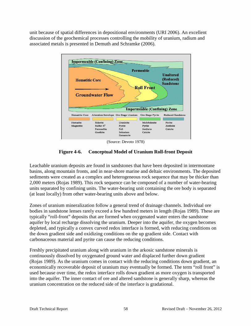
unit because of spatial differences in depositional environments (URI 2006). An excellent discussion of the geochemical processes controlling the mobility of uranium, radium and associated metals is presented in Demuth and Schramke (2006).
(Source: Devoto 1978)
Figure 4-6. Conceptual Model of Uranium Roll-front Deposit
Leachable uranium deposits are found in sandstones that have been deposited in intermontane basins, along mountain fronts, and in near-shore marine and deltaic environments. The deposited sediments were created as a complex and heterogeneous rock sequence that may be thicker than 2,000 meters (Rojas 1989). This rock sequence can be composed of a number of water-bearing units separated by confining units. The water-bearing unit containing the ore body is separated (at least locally) from other water-bearing units above and below. Zones of uranium mineralization follow a general trend of drainage channels. Individual ore bodies in sandstone lenses rarely exceed a few hundred meters in length (Rojas 1989). These are typically “roll-front” deposits that are formed when oxygenated water enters the sandstone aquifer by local recharge dissolving the uranium. Deeper into the aquifer, the oxygen becomes depleted, and typically a convex curved redox interface is formed, with reducing conditions on the down gradient side and oxidizing conditions on the up gradient side. Contact with carbonaceous material and pyrite can cause the reducing conditions.
Freshly precipitated uranium along with uranium in the arkosic sandstone minerals is continuously dissolved by oxygenated ground water and displaced further down gradient (Rojas 1989). As the uranium comes in contact with the reducing conditions down gradient, an economically recoverable deposit of uranium may eventually be formed. The term “roll front” is used because over time, the redox interface rolls down gradient as more oxygen is transported into the aquifer. The inner contact of ore and altered sandstone is generally sharp, whereas the uranium concentration on the reduced side of the interface is gradational.
Draft Technical Report 58 Revised Draft – November 26, 2012

The depth of the ore body varies significantly from site to site. Ore bodies in the Texas Gulf Coastal Plain tend to be shallow-lying, while those in the Wyoming Basin show considerable variability, as illustrated by the following:
• Burns/Moser TX (Lower Oakville) – 230 to 280 ft (http://www.wise-uranium.org/udusail.html#KINGSV).
• Clay West TX (Lower Oakville) – 250 to 400 ft (http://www.wise-uranium.org/udusail.html#KINGSV).
• Crow Butte (Basal Chadron) – 400 to 800 ft (NRC 1998).
• Dewey-Burdock (Lakota and Fall River) – 500 to 800 ft (Dewey); 300 to 500 ft (Burdock) (SRK 2011).
• Irigaray WY – 100 to 300 ft (Irigary 2004).
• Palangana TX (Goliad Formation) – 230 to 390 ft (http://www.wise-uranium.org/udusail.html#PALANGANA).
• Smith Ranch/Highlands, A-Wellfield WY (20-Sand) – 530 ft avg (Kearney 2004).
• West Cole TX (Soledad member of Catahoula Formation) – 225 to 270 ft (http://www.wise-uranium.org/udusail.html#WESTCOLE).
• Zamzow TX (Oakville sand) – 35 to 225 ft (http://www.wise-uranium.org/udusail.html#ZAMZOW).
It is expected that deeper lying ore bodies will be less susceptible to seasonal variations in ground water chemistry associated with areal recharge than shallower ore bodies.
4.2 Aquifer Exemption Requirement An aquifer exemption is required if the proposed injection zone is an underground source of drinking water. Applicants submit a Petition for Aquifer Exemption to the state for review. Although the state reviews the aquifer exemption petition, it cannot grant the final aquifer exemption. After the state makes a decision on the aquifer exemption petition and it is duly public noticed, the state makes a recommendation of the decision to EPA. EPA makes the final decision regarding aquifer exemptions. As part of the aquifer exemption Petition, the Applicant must evaluate potential impacts on the water resources in the vicinity of the proposed mine. This evaluation generally involves water quality and use surveys within at least a 2-mile radius of the site. Water level measurements and ground water samples collected during this phase of the application process often provide some of the earliest baseline data. 4.3 Establishing Baseline Conditions Before initiating leaching activities, knowledge of the aquifer baseline characteristics is needed to help determine restoration goals for the post-mining phase. Pre-mining monitoring and testing wells are installed to collect data that define the ground water flow regime through the extraction
Draft Technical Report 59 Revised Draft – November 26, 2012

zone and surrounding areas and determine the chemical characteristics of the ground water. Monitoring wells should be installed at well locations up gradient, down gradient, and tangential to the proposed ISR field, as well as within the “ore-zone.” Well placement should be designed to measure all potential “escape” pathways for introduced constituents and mobilized metals, as well as to provide data to determine the choice and effectiveness of aquifer restoration actions. Selected up gradient and down gradient wells outside the wellfield should be continuously monitored throughout all phases of the operation illustrated in Figure 3-1. This will provide data that may assist in interpreting changes in ground water chemistry within the wellfield during steady state and long-term stability monitoring and possibly to detect seasonal variations in ground water chemistry in shallow deposits. The design of the monitoring network is largely a site-specific decision predicated on a thorough knowledge of the ground water flow regime and the effects of the injection and withdrawal rates on the flow system behavior. A system of wells should be emplaced to monitor the horizontal and vertical ground water velocity and flow paths, the ground water chemical conditions, and the potential for hazardous constituents to migrate beyond the ISR mine field, both within the mined aquifer and through transmission of contamination to overlying and underlying aquifers. These areas beyond the ISR may experience contamination from the mined area. The following components and parameters need to be considered in establishing baseline site characteristics (see Section 3.5, and particularly Table 3-3, for more details on analytes to be monitored in ground water):
(1) Hydrogeochemical Conditions – Eh (including redox-sensitive couples), dissolved oxygen, pH, major ions, TDS, carbonate alkalinity, pCO2, radioactive constituents, colloids, organic constituents, hydrogen sulfide, trace elements (to be compared against post-restoration measurements).
(2) Concentrations of those constituents listed in 40 CFR Part 192 – arsenic, barium, cadmium, chromium, lead, mercury, molybdenum, nickel, Ra-226 and Ra-228, selenium, silver, uranium, etc.
(3) Uranium Ore Deposit Types and Oxidation States – The site-specific and varied diagenic processes that formed the uranium deposits will determine how ISR operations will affect baseline conditions and which restoration approach is likely to be most effective. Knowledge of these processes can be used as a framework in estimating the time needed for the aquifer to reach baseline conditions once post-mining restoration and monitoring are initiated.
(4) Hydrogeologic Setting – Pre-mining ground water velocities (unstressed), flow paths, and solute transport time frames. A reliable and defensible characterization survey of the ISR site requires thorough core and water sampling from all monitoring wells and exploration boreholes. Sufficient data must be collected before the mining activity commences to understand when baseline levels have been reached after mining. Aquifer pump/stress tests and core sample analysis will determine aquifer characteristics within and surrounding the ore body and be used to determine:
a. Host rock and ore zone permeability, porosity, storativity, and thickness
Draft Technical Report 60 Revised Draft – November 26, 2012

b. Whether more monitoring wells are needed for postclosure activities and to assess the time frame of postclosure monitoring
c. Time frame estimates after mining has ceased, in order for the system to reach pre-ISR conditions
d. Recharge/discharge points
e. Impermeable layers above and below the ore zone
f. Proximity to ground water barriers
g. Proximity to surface water bodies – natural or manmade Sampling the ground water may require special sample collection techniques, depending on the chemical constituents of concern. For major ions and some other chemical species, sampling may be relatively simple, in that these species are not susceptible to change upon exposure to atmospheric conditions. For species that are susceptible to re-equilibration in response to atmospheric conditions, particularly redox-sensitive species and the carbonate-bicarbonate system, water sampling may require that the sampled interval be “packed off” within the well and water samples taken in containers, which were placed within the sealed intervals prior to the “packing-off” and left to equilibrate in the flowing ground water for a period of time before removal. Redox-sensitive couples typically examined include ferrous (II)/ferric (III) iron, and the arsenic (III) /arsenic (V) couple. In addition to dissolved oxygen levels, these couples can produce important characterization of the redox conditions in the production zone before, during, and after the leaching process and can also be important in determining the effectiveness of various aquifer restoration processes. In addition, uranium speciation is strongly affected by pH and carbonate concentrations in the ground water, which, in turn, are a function of the pCO2 in the ground water. Exposure of the ground water sample to the atmosphere can result in the escape of CO2 and re-equilibration of the uranium-carbonate system due to the out-gassing. Then the uranium concentrations in the reequilibrated water would not reflect the actual speciation in situ, and, consequently, could result in misleading calculations of uranium speciation and solubility constraints in the subsurface waters. Because of these effects and their relative importance to characterizing the in-situ ground water chemistry, monitoring water chemistry in and around the “ore body” may well require differing sampling methods.
Figure 4-7 illustrates the spatial variability that exists between the ore zone and its surroundings. The figure summarizes results for pre-mining sampling of excursion monitor wells (designated as EM) and production zone wells (EMP) for Wellfield H-E at the Highland uranium project in Wyoming (Hoy 2006). Within the production zone, most of the baseline wells showed elevated concentrations of uranium and radium as compared to the excursion monitor wells located a few hundred feet from the production zone wells. Within the production zone, radium (Ra-226) was generally >100 picocuries per liter (pCi/L), while at the excursion monitor wells, Ra-226 was generally <5 pCi/L. Uranium was generally >0.03 mg/L in production zone baseline wells, while it was always <0.030 mg/L in the baseline monitor wells. The median uranium concentration was about 0.04 mg/L within the production zone and about 0.015 mg/L in the monitor ring. It is possible that different geochemical conditions within the ore zone, as compared to the host rock,
Draft Technical Report 61 Revised Draft – November 26, 2012

precluded the movement of uranium and radium down gradient. (See also Figure 4-4 and Figure 4-6.) The wide variablitity and sharp concentration gradients of background uranium concentrations observed at the Rosalita ISR project are shown in Figure 4-8 (URI 2010). The isolated areas of elevated uranium concentrations within the ore body present a challenge to establishing statistically representative background concentrations as described below in Section 4.2.1. Recent studies (Hall 2009; NRDC 2012), as well as administrative hearings for the Goliad ISR aquifer exemption that took place in 2010, have focused attention on a lack of guidance on statistical establishment of background levels for hazardous constituents in ground water, and selective use of well data, which could distort the chosen background levels for restoration. Use of statistics in setting these numbers is discussed further in Section 7 of this report.
Draft Technical Report 62 Revised Draft – November 26, 2012

Source: Hoy 2006
Figure 4-7. Well and Production Zone Locations and Baseline Concentrations of TDS, Uranium, and Radium –Wellfield H-E
Draft Technical Report 63 Revised Draft – November 26, 2012
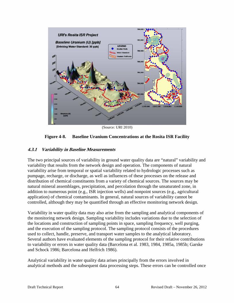
(Source: URI 2010)
Figure 4-8. Baseline Uranium Concentrations at the Rosita ISR Facility
4.3.1 Variability in Baseline Measurements The two principal sources of variability in ground water quality data are “natural” variability and variability that results from the network design and operation. The components of natural variability arise from temporal or spatial variability related to hydrologic processes such as pumpage, recharge, or discharge, as well as influences of these processes on the release and distribution of chemical constituents from a variety of chemical sources. The sources may be natural mineral assemblages, precipitation, and percolation through the unsaturated zone, in addition to numerous point (e.g., ISR injection wells) and nonpoint sources (e.g., agricultural application) of chemical contaminants. In general, natural sources of variability cannot be controlled, although they may be quantified through an effective monitoring network design. Variability in water quality data may also arise from the sampling and analytical components of the monitoring network design. Sampling variability includes variations due to the selection of the locations and construction of sampling points in space, sampling frequency, well purging, and the execution of the sampling protocol. The sampling protocol consists of the procedures used to collect, handle, preserve, and transport water samples to the analytical laboratory. Several authors have evaluated elements of the sampling protocol for their relative contributions to variability or errors in water quality data (Barcelona et al. 1983, 1984, 1985a, 1985b; Garske and Schock 1986; Barcelona and Helfrich 1986). Analytical variability in water quality data arises principally from the errors involved in analytical methods and the subsequent data processing steps. These errors can be controlled once
Draft Technical Report 64 Revised Draft – November 26, 2012
suitable water quality indicators or chemical constituents have been selected and a thorough data quality assurance/quality control program has been designed and executed. Optimization of sampling frequency in ground water quality monitoring networks should provide sufficient sensitivity for chemical constituent detection and adequate characterization of average chemical conditions. This should be accomplished with a minimum number of sampling times, but this sampling should provide important information for determining the adequacy of restoration and necessitates a high degree of confidence. This may then require more lengthy sampling periods. The hydrology of the ground water system will influence the impact of the sources of variability mentioned above. Although aquifer hydraulic properties may not vary significantly at a single measurement point over time, spatial variability may be substantial. This is a very active area of research with application to monitoring network design (Christensen and Doherty 2008, Meyer et al. 2007, Cooley 2004, Doherty and Hunt 2009). Results of such research will be important for determining the efficacy of restoration efforts and regulatory decisionmaking about the long-term stability of the restored wellfield. Temporal and spatial variations in ground water elevation may affect ground water flow rate and the direction of movement. Such changes may influence the quality of the ground water in the vicinity of a sampled well by directing water from a different up gradient area or changing the velocity with which dissolved constituents move along a flow path. Examples abound in the literature detailing ground water response (i.e., elevation change) to a wide variety of influences. In addition to seasonal fluctuations produced in response to short-term (i.e., months to 1 year) events, ground water levels also reflect changes in long-term (i.e., years to decades) conditions. Natural and artificial (man-induced) influences can cause changes in ground water elevation, including natural (e.g., rainfall and snowmelt) and artificial recharge (e.g., pipe leaks, injection wells) and natural (e.g., evapotranspiration) and artificial discharge (e.g., pumping). These variations may be important in situations where multiple ore zones are mined sequentially, and decisions on when and where restoration efforts are to be carried out and regulatory decisions on these efforts must be made.
Ground water quality monitoring networks are designed for a number of purposes, including ambient resource studies, contaminant detection and assessment, contaminant source evaluation, and research investigations. The effective design of virtually any such network, regardless of purpose, depends on knowledge of the hydrogeologic system of interest, an indication of the presumed contaminants or preferred water quality indicators, and an assessment of the relative contributions of sources of variability. These aspects of monitoring network design have been addressed in the literature (Todd et al. 1976, Sanders et al. 1983, Moss et al. 1978, Liggett 1984, Liggett 1985, Gillham et al. 1983). The common recommendation in these works is that background information must be supplemented with the results of a preliminary sampling to progressively refine the network design to account for error and variability in the chemical results. Variability in the analytical results for particular ground water chemical constituents may arise from “natural” causes such as nonhomogeneous spatial distributions of the constituents and temporal variability in recharge. Variability may also arise due to network design-related factors
Draft Technical Report 65 Revised Draft – November 26, 2012

such as well design, sampling devices, and sampling protocols. The apparent sources of variability in water quality data, which are often attributed to natural (i.e., temporal and spatial) effects, include hydrologic transience, the fluctuations in contaminant source strength and composition and the interactions between reactive chemical, biochemical, and mineral constituents in recharge water and ground water. A detailed understanding of the interdependence of hydrologic, biological, and chemical processes in the subsurface is limited. However, it may not be necessary to fully understand the relationship between these processes, contaminant sources, and the resultant chemical distributions in order to establish representative background concentrations, monitor potential contaminant releases (e.g., excursions), and predict remediation times. The temporal and spatial variability, which is observed in water quality results over time at discrete monitoring points, is the result of the processes noted in the preceding discussion, as well as the sample collection and measurement errors inherent to network design and operation. This variability, or “noise,” in the data encompasses the stochastic distribution of possible values for particular chemical constituents and the effects of both determinate (i.e., systematic) and indeterminate (i.e., random) error. Determinate error can be measured as inaccuracy or bias if the “true value” is known. Indeterminate error can be estimated as imprecision or irreproducibility if enough replicate determinations can be made to faithfully estimate the mean or the “true” value. In practice, determinate errors can be estimated and controlled only by careful quality assurance/quality control measures exercised over appropriate sampling and analytical procedures because the true value in environmental distributions is unknown, and some disturbance of the subsurface is inevitable in ground water quality work. Identifying and controlling these design-related errors are described in several sources (Barcelona et al. 1983, Barcelona et al. 1985a, Barcelona 1988, Barcelona et al. 1986, Barcelona and Gibb 1986, Puls and Barcelona 1996, and EPA 2010d). Statistical measures of short-term temporal variability include seasonal effects (e.g., consequences of recharge or temperature effects), which can be assigned to the seasons of the year, periodic effects (e.g., consequences of anthropogenic contaminant sources or pumping effects), and serial correlation or dependence effects, which tend to make data points following maxima or minima in temporal data series higher or lower, respectively, than one would attribute to random processes alone. Trends in data, on the other hand, are long-term variations compared to those that may occur within a hydrologic year (Porter and Trautman 1984). This categorization of temporal effects is somewhat artificial in that the combination of seasonal, periodic, or correlative components may result in a water quality time series that cannot be differentiated quantitatively. Because of this factor, the identification of short- or long-term trends in water quality is conditional on some knowledge of the proximity of the sampling location to the location and time of chemical release, as well as the statistical characteristics of ground water quality variables. Statistical measures of temporal variability have been reviewed by Loftis et al. (1986), Montgomery et al. (1987), and Harris et al. (1987). They cite numerous examples of both short- and long-term temporal variability, which supplement the earlier reviews of Porter and Trautman (1984) and Colchin et al. (1978). The Air Force Center for Environmental Excellence (AFCEE) has also developed two computer software packages that employ sophisticated
Draft Technical Report 66 Revised Draft – November 26, 2012
geostatistical/ statistical analysis algorithms to facilitate the optimization and termination of current long-term monitoring (LTM) programs (Aziz et al. 2006). The Monitoring and Remediation Optimization System (MAROS) software assists in optimizing monitoring networks both spatially and temporally. A recent development in MAROS is the addition of the Modified Cost-Effective Sampling (CES) Method, which is designed to set the sampling frequency for a well based on the analysis of time series concentration data at each sampling location, considering both recent and long-term trends of the concentration data. In contrast to the spatially based Delaunay Method originally used in the MAROS sample location optimization, the Modified CES Method is based on temporal analysis. Its use, combined with the Delaunay Method and trend analyses, leads to a comprehensive process of sampling optimization. The second program developed by AFCEE is the geostatistical temporal/spatial (GTS) optimization algorithm, which is a robust and powerful computer application designed for use by mid-level geostatisticians. GTS software can optimize individual input data sets for LTM networks containing analytical data from more than one aquifer or hydrogeologic unit (MAROS can optimize only a single hydrogeologic unit). Additional technical information, user’s manuals, and executable computer code for MAROS and GTS can be obtained from the AFCEE website. Section 7.0 provides a more detailed discussion of the statistical approaches to address both spatial and temporal variability. A sufficiently high sampling frequency (i.e., quarterly) is required to statistically distinguish seasonal effects from those of serial dependence or autocorrelation (Loftis et al. 1986). In many instances, limited ground water quality data sets, combined with quality variables that are frequently not normally distributed, constrain the use of simple parametric statistical tests of significance to compare means or identify trends (Montgomery et al. 1987). The adoption of a minimum sampling frequency of “quarterly” can be useful during the characterization phase of ground water monitoring to evaluate seasonality, rate of change and variability, especially for fast-moving plumes. However, for more stable plumes, the default adoption of quarterly monitoring may be determined to be unnecessary if long-term monitoring can demonstrate no harm by utilizing longer intervals. Conversly, if variability in the ground water compositions is relatively high and the concentrations of the analyte of concern over time is changing slowly, more frequent sampling may be necessary to define the presence or absence of trends with a reasonably high degree of confidence (see Sections 7.7 and 7.8 for an example of these situations). The use of sampling intervals ranging from quarterly, semiannual, annual, to biennial levels is very common in long-term ground water monitoring (Air Force 1997; NFESC 2000).
Spatial and temporal variability in ground water quality may affect the sensitivity of contaminant detection and the estimation of mean chemical concentrations. To some extent, spatial chemical data collected at discrete points along a horizontal flow path may be quite similar to data collected over time at a single point in the path. This supposition depends, of course, on a number of factors related to hydrologic conditions, as well as the nature of the chemical source, reactivity, and mobility constraints. The substitution of spatially intense samples for use in temporal variability studies could be applied to studies of ambient concentrations of conservative chemical species for regional assessments in unique hydrologic situations.
Draft Technical Report 67 Revised Draft – November 26, 2012
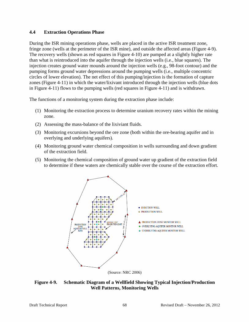
4.4 Extraction Operations Phase During the ISR mining operations phase, wells are placed in the active ISR treatment zone, fringe zone (wells at the perimeter of the ISR mine), and outside the affected areas (Figure 4-9). The recovery wells (shown as red squares in Figure 4-10) are pumped at a slightly higher rate than what is reintroduced into the aquifer through the injection wells (i.e., blue squares). The injection creates ground water mounds around the injection wells (e.g., 98-foot contour) and the pumping forms ground water depressions around the pumping wells (i.e., multiple concentric circles of lower elevation). The net effect of this pumping/injection is the formation of capture zones (Figure 4-11) in which the water/lixivant introduced through the injection wells (blue dots in Figure 4-11) flows to the pumping wells (red squares in Figure 4-11) and is withdrawn. The functions of a monitoring system during the extraction phase include:
(1) Monitoring the extraction process to determine uranium recovery rates within the mining zone.
(2) Assessing the mass-balance of the lixiviant fluids.
(3) Monitoring excursions beyond the ore zone (both within the ore-bearing aquifer and in overlying and underlying aquifers).
(4) Monitoring ground water chemical composition in wells surrounding and down gradient of the extraction field.
(5) Monitoring the chemical composition of ground water up gradient of the extraction field to determine if these waters are chemically stable over the course of the extraction effort.
(Source: NRC 2006)
Figure 4-9. Schematic Diagram of a Wellfield Showing Typical Injection/Production
Well Patterns, Monitoring Wells
Draft Technical Report 68 Revised Draft – November 26, 2012

(Source: Gard and Mahoney 2012)
Figure 4-10. Example of MODFLOW Predicted Potentiometric Surface during Active
Mining
(Source: Gard and Mahoney 2012)
Figure 4-11. Example of MODPATH Predicted Flow Paths During Active Mining
Draft Technical Report 69 Revised Draft – November 26, 2012
4.5 Post-extraction Phase The post-extraction monitoring system should be designed to assess the effectiveness of the remediation process, assess when final remediation objectives have been met, and assure that the affected aquifer is at steady state, long-term stability has been demonstrated, and the site is ready for decommissioning. A system of wells located in the active treatment zone, as well as outside the boundary of the affected area, is required to monitor the horizontal and vertical ground water velocity and flow paths in the vicinity of the ISR site. The functions of a post-mining monitoring system include:
(1) Measuring ground water chemical constituents to determine if and/or when the ground water chemistry has returned to pre-ISR (baseline) compositions.
(2) Determining if additional chemical components have been added to the ground water as a product of the extraction process (e.g., metals mobilized with the uranium).
(3) Demonstrating when the ground water chemistry has reached “stable” levels (i.e., statistically equivalent compositions over an extended time period).
(4) Determining if post-mining restoration levels for ground water constituents have been met.
4.6 Factors Affecting Post-mining Time Frames and Wellfield Stability Post-restoration monitoring must be of sufficient duration to ensure that once ground water chemistry appears to have reached acceptable restoration levels, these levels are at steady state and the ground water system is at equilibrium. Steady-state restoration levels are not just for uranium, but also for other hazardous constituents that may have been mobilized by ISR operations, such as radium, manganese, and selenium. Chemical speciation and solubility, as well as natural attenuation processes, must be understood in order to determine when the affected aquifer has reached a steady-state condition. Both geochemical and advective-dispersive modeling should be used as tools to assist in designing the most effective means of restoring the aquifer. The approach that is generally taken to couple the geochemical processes with ground water flow and contaminant transport is to first use MODFLOW to create a calibrated flow field that reasonably resembles the actual field conditions. Once the flow conditions are established, a transport code (e.g., MT3D) is applied to simulate simple geochemical behavior (e.g., sorption). A more complex geochemical code is then applied (e.g., PHT3D) to simulate reactive transport and surface complexation. The environmental chemistry of uranium is largely dictated by its oxidation state; the solubility, and therefore mobility, of uranium is greatest when it is in the U(VI) state. Because different chemicals may be used during the restoration process than were used during ISR operation, the chemical form of uranium or other hazardous constituents may differ during restoration. Since most of the available computer codes do not have a method of calculating reaction rates, these reactions may be unexpected, and the monitoring program must last long enough to accommodate such unexpected conditions. There are a few sophisticated codes, however, that allow the reactive transport processes to be coupled to the ground water flow regime, such as PHAST or PHT3D. These codes have intensive data requirements, and EPA recognizes the
Draft Technical Report 70 Revised Draft – November 26, 2012

importance of understanding the geochemical processes and has entered into a corporative agreement with the U.S. Geological Survey under a Regional Applied Research Effort (RARE). The main objective of this work is to provide a predictive model that describes the ground water flow and geochemical changes along with longer-term transport of dissolved constituents during and after the uranium ISR mining process (see also Section 4.3.7 below). One of the most important factors affecting restoration times is that there may be significant quantities of uraninite remaining after mining is complete (Figure 4-12). Post-mining sampling and core analysis, as well as more complete tracking of the water balance and uranium mass removal rates during mining, would assist in designing a more effective restoration. Another factor affecting the post-monitoring time frame and wellfield stability is the form of remediation used. Pump and treat techniques are common remediation approaches. One consideration, however, are the large volumes of water required when pump and treat technologies are used to restore the aquifer to pre-mining conditions. Issues related to both water quality and quantity have resulted in EPA denying the Applicants Aquifer Exemption Request until additional work is performed at the Goliad mine in Texas to demonstrate that nearby water resources will not be adversely impacted for the next 75 years (EPA 2012).
(Source: Gard and Mahoney 2012)
Figure 4-12. Example of PHT3D Predicted Post-mining Uraninite Concentrations
Geochemically based methods are promising as potential remedial alternatives, in that significantly less water could be used during site restoration since strong reducing agents (e.g., hydrogen sulfide) are injected to induce chemical precipitation of the uranium from solution. Monitored natural attenuation is another response action that may be effective in certain situations. Natural attenuation processes include a variety of physical, chemical, and biological processes that can act to reduce the mass, mobility, volume, or concentration of contaminants in ground water. Attenuation mechanisms important at ISR sites are described in Table 3-4 and include processes such as pH buffering and acid neutralization, adsorption at the mineral-water interface, mineral precipitation, dilution, and biological activity.
Draft Technical Report 71 Revised Draft – November 26, 2012
Pump and Treat Alternative approaches included in pump and treat remediation are:
• Ground Water Transfer – This involves transferring ground water between the wellfield starting restoration and another wellfield where uranium leach operations are beginning. No liquid effluents are generated as water is transferred between one wellfield and another.
• Ground Water Sweep – Injection of lixiviant is stopped, and the contaminated liquid is pumped from the leaching zone via all of the injection and production wells. Fresh ground water flows into the leaching zone from the outside, which displaces lixiviant in the pore spaces. Typically, an ion-exchange system is used to process the sweep water, which is disposed of either in evaporation ponds or via a deep injection well in accordance with the site permit. The pumping rates are site specific, and the duration and volume of water removed depend on the aquifer affected by the ISR. Due to heterogeneities in the aquifers, ground water sweep alone may be insufficient and uneconomical for complete restoration. In addition, ground water sweep may create oxic conditions when up gradient waters enter the ore zone, making it more difficult to re-establish chemically reducing conditions.
• Reverse Osmosis (RO) – To return ground water to baseline conditions, it is usually necessary to remove contamination from the mined zone water while minimizing disposal of waste liquids. RO, which involves passing the water being restored through pressurized, semipermeable membranes, is a common way of treating ground water. The RO treatment results in clean water or permeate that can be reinjected into the aquifer and brine that is water with concentrated ions. The brine is usually sent to an evaporation pond, injected into deep disposal wells, or dried (using an evaporator) for subsequent disposal at a licensed facility.
• Permeate Injection – Many aquifers are characterized by porosity where ground water with decreased mobility resides in regions of moderate to low permeability. It is very difficult to remove all of the lixiviant and associated contamination from this portion of the ground water, which will act as a source of contaminants, even after long periods of pumping and treating.
Geochemically Based Techniques Another component of aquifer restoration is accomplished by establishing a chemical environment that alters the solubility of dissolved constituents. Chemicals may be added to injection water in the latter stages of restoration to assist in re-establishing baseline conditions. These methods typically invoke chemical reactions in which some species are reduced to a lower valence state. Addition of reagents such as hydrogen sulfide and sodium hydrosulfide tend to convert dissolved species such as uranium, selenium, molybdenum and arsenic to a lower valence state with attendant reductions in solubility (NRC 2007, p. 17).
Draft Technical Report 72 Revised Draft – November 26, 2012
Monitored Natural Attenuation Monitored natural attenuation (MNA) refers to the reliance on natural processes to achieve site-specific remediation objectives within a reasonable time frame. These processes include biodegradation, dispersion, dilution, sorption, and volatilization; radioactive decay; and chemical or biological stabilization, transformation, or destruction of contaminants. The overall impact of MNA at a given site can be assessed by evaluating the rate at which contaminant concentrations are decreasing either spatially or temporally. However, USGS has suggested a note of caution regarding the efficacy of natural attenuation (NRC 2007, p. 17):
Because the ore zone typically is under chemically reducing conditions prior to mining, it has frequently been argued or assumed that the natural reducing conditions will return over a period of time. However, it is difficult to predict how much time is required or even if the reducing conditions will be returned via natural processes. The mining disturbance introduces a considerable amount of oxidant to the mined region and may oxidize all the pyrite associated with the original ore zone.
EPA has prepared a technical resource document (EPA 2007a and 2007b) that presents a four-tiered assessment of MNA as a viable response action for selected metal, metalloid, and radionuclide contaminants encountered in ground water. The assessment involves the following: (1) demonstrating contaminant sequestration mechanisms; (2) estimating attenuation rates; (3) estimating attenuation capacity of aquifer solids; and (4) evaluating potential reversibility issues. EPA has a number of guidance documents that pertain to MNA (e.g., EPA 1999b) and specifically to radionuclides (EPA 2010a). Section 6.4 of this report presents additional details on MNA. 4.7 Modeling 4.7.1 Objectives and Conceptual Model Development Modeling of ground water flow, contaminant fate and transport, and chemical speciation is often utilized to predict the spatial and temporal behavior of the hydrogeochemical system. Ground water flow and geochemical modeling is commonly implemented to assist in meeting different objectives during each phase of the ISR process as described below: Pre-Mining
• Establish background concentration of important ground water constituents and determine geochemical constraints that may control contaminant concentrations, e.g., solubility constraints.
Draft Technical Report 73 Revised Draft – November 26, 2012

Active Mining
• Determine spacing of injection and pumping wells.
• Optimize the monitoring well spacing to detect injection fluid excursions into non-mined aquifer zone(s).
Aquifer Restoration
• Evaluate changes to hydraulic conductivities, gradients and flow directions.
• Estimate the number of pore volumes needed during site remediation activities to adequately reduce contaminant concentrations.
• Estimate remediation times.
• Predict potential off-site impacts on water levels and quality. Post-Remedial Monitoring
• Evaluate the long-term stability of the contaminants within the mined area, as well as any that have migrated further down gradient.
• Establish a specific period of monitoring for ISR facilities once uranium extraction operations are completed.
Prior to starting remediation of in-situ leach mining sites, modeling can be used to predict the behavior of the ground water system during and after ground water restoration. To make such a prediction, a conceptual model must be formulated that includes the most important physical and geochemical processes that are occurring in the system at the end of restoration and that will occur in the system in the future. In formulating such a model, three fundamental processes must be included: ground water flow, solute transport, and chemical reactions. Secondary processes such as microbial degradation may also be considered. Microbial action may not be important during restoration since the ground waters are being moved through the system rather quickly, but may have a more important role when the pumps stop and long-term stability is evaluated. In addition, the initial conditions of certain physical and chemical variables in the system must be specified, as well as any known changes to these variables that may occur in the future. It is important to recognize that a model is only a tool for approximating a field system. Data collected during pilot studies at an ISR field site should be useful in constructing the conceptual model. For a ground water flow system, the nature of the conceptual model will determine the dimensions of the physical model and the design of a grid for numerical calculations. It is important to distinguish between the conceptual model of the hydrogeologic system and a computer code. A computer code is a set of instructions for performing calculations, whereas the conceptual model represents the physical and chemical understanding of the system.
Draft Technical Report 74 Revised Draft – November 26, 2012
4.7.2 Ground Water Flow and Contaminant Transport Modeling After the conceptual model is developed, a computer code may be used to simulate the controlling processes that affect ground water flow and chemical transport. Computer modeling frequently used to meet the performance objectives at ISR facilities includes five primary types: (1) ground water flow, (2) advective-dispersive transport, (3) advective transport (i.e., particle tracking – no dispersion), (4) geochemical speciation, and (5) reactive-transport modeling. These modeling approaches are described in greater detail below and in Section 4.7.3. The ground water flow and advective transport modeling typically performed for ISR sites use finite-difference techniques, which require that the ground water system be divided (“discretized”) into finite-sized blocks or “cells.” Each cell is assigned unique hydraulic properties depending on the available field data and the goals for the analysis. In this way, the model can accommodate complex features of the ground water system. The time represented by the modeling effort must also be divided into discrete periods or “time steps.” These steps must be short enough to provide an accurate solution, but not so short that they require an excessive number of calculations to run a simulation. The finite-difference method also requires that values for hydraulic head be assigned at flow boundaries (referred to as “boundary conditions”), as well as for the initial time period of the simulation (referred to as “initial conditions”). This is a requirement for producing a unique solution with any numerical method that depends on iteration, as does the finite-difference method. The most popular computer code to simulate ground water flow is MODFLOW2000 (Harbaugh et al. 2000). The output from this code is a three-dimensional flow field (an array of hydraulic head elevations) representing average conditions in the model area. Once the flow field is established, the most widely used contaminant transport code, MT3DMS is used to predict future concentrations of selected constituents at ISR facilities (Zheng and Wang 1999). MT3DMS does not explicitly simulate geochemical reactions but can be used to simulate changes in concentrations of miscible contaminants in ground water, while considering advection, dispersion, diffusion, and some aggregate chemical reactions (i.e., distribution coefficient), with various types of boundary conditions and external sources and/or sinks. The basic chemical reactions included in the model are equilibrium-controlled or rate-limited linear or nonlinear sorption, and first-order irreversible or reversible kinetic reactions. Somewhat more sophisticated, multispecies chemical reactions can be simulated by add-on reaction packages. MODFLOW2000 and MT3DMS are commonly applied at ISR facilities to evaluate how the average flow field, together with other transport parameters, affects chemical movement in ground water and plume development from lixiviant sources. The chemical transport model is often used to simulate the expansion of the plume, during both the time of active leaching activities and the post-closure stage. If diffusive and dispersive processes are not important to the transport analysis, the computer code MODPATH is frequently used to compute three-dimensional advective flow paths. The code uses output from steady-state or transient ground water flow simulations from MODFLOW. MODPATH is described in USGS Open-File Report 94-164 (Pollock 1994). MODPATH uses a
Draft Technical Report 75 Revised Draft – November 26, 2012

semianalytical particle tracking scheme that allows an analytical expression of the particle’s flow path to be obtained within each finite-difference grid cell. Particle paths are computed by tracking particles from one cell to the next until the particle reaches a boundary, an internal sink or source, or satisfies some other termination criterion. After the modeling objectives are defined (Section 4.7.1), modeling of the ground water flow and contaminant fate and transport generally follows the set of steps detailed below:
(1) Developing a conceptual model to guide creation of model attributes.
(2) Selecting an appropriate computer code(s) for the analysis.
(3) Establishing the time period represented by the model and the duration of subdivisions of this period (time steps) required for modeling.
(4) Selecting a suitable model domain and determining the dimensional (horizontal and vertical) limits of the analysis.
(5) Establishing the model structure by determining the number of model layers and the grid spacing requirements for the flow analysis.
(6) Incorporating hydraulic boundaries and features, including the shape and characteristics of constant-head boundaries, precipitation/recharge, and pumping/injection.
(7) Assigning hydraulic conductivity values.
(8) Specifying initial head values (ground water surface elevation).
(9) Evaluating and assigning appropriate model computational characteristics (e.g., solution method, iteration limits, and convergence criteria) to enhance model stability, computational efficiency, and solution accuracy.
(10) Evaluating the sensitivity of model results to changes in model parameters.
(11) Establishing the model structure, including determining the number of model layers and the grid spacing requirements for the transport analysis.
(12) Assigning the characteristics of chemical sources (e.g., lixiviant), consisting of dimensions, locations, concentrations, and time dependency.
(13) Assigning transport parameters, including the distribution coefficients, dispersivities, and porosities.
(14) Defining chemical interactions among dissolved and solid phases.
(15) Developing remedial design scenarios and conducting chemical transport simulations and exporting the observed concentrations at prespecified locations.
(16) Post-processing the data with Graphical User Interface (GUI) tools.
Although the ISR method of uranium mining has a less disruptive overall environmental impact compared to open-pit mining, this mining method significantly alters the ground water chemistry and flow patterns during mining. One of the common strategies at all of the ISR facilities is to better understand the most probable fate and transport of uranium and other constituents during
Draft Technical Report 76 Revised Draft – November 26, 2012
and after ISR operations. To achieve this goal, mathematical modeling of chemical reaction kinetic equations or equilibrium thermodynamic equations can be used to describe chemical interactions among dissolved chemical species, the dissolution of immobile solid phases, or the formation and precipitation of new, immobile solid phases. The following section presents a more detailed discussion of the role that geochemical modeling plays in the understanding of important chemical processes at ISR facilities. 4.7.3 Geochemical Modeling Geochemical reactions along ground water flow paths can lead to regional variations in water composition that evolve in the direction of flow. Iso-concentration contours of reacting dissolved constituents drawn on maps of water composition tend to align perpendicular to the direction of ground water flow. It is these geochemical reactions that have created the sandstone-hosted uranium roll-front deposits along the interface between oxidized and reduced sandstones. The geochemistry associated with these deposits is complex and variable. The deposits contain a mixture of U+6 minerals on the oxidized side of the front and reduced U+4 minerals on the reduced side of the front (Harshman 1974). Oxidizing ground water flowing through sandstones transports uranium U+6 in solution down dip until reductants in the host sandstones precipitate uranium as U+4 minerals. Associated elements are often found distributed across the roll in zones determined by their redox potential and solubility in alkaline, oxidizing ground water that comes into contact with pH neutral, reducing sediments at the reaction front (Deutsch et al. 1985; Harshman 1972). Ground water within the ore zone of roll-front deposits often contains high concentrations of uranium and its daughter products, as well as elevated selenium, arsenic, lead, and other dissolved constituents (Johnson et al. 2010). Modeling of any type does not lead to a unique solution, but the number of possibilities are reduced with greater amounts of carefully collected field data. Martin et al. (2005) summarized the benefits and limitations of geochemical modeling as follows:
Benefits
• Provide insight into potential future conditions. • Determine which variables are most important in determining future
conditions. • Assess potential effects of uncertain parameters. • Establish objectives and test conditions for field and laboratory studies. • Integrate available information.
Limitations
• Insufficient input data. • Modeling can be challenging and results misinterpreted. • Uncertain and variability of the results. • Difference between modeled and actual field conditions.
Draft Technical Report 77 Revised Draft – November 26, 2012

Approaches to Geochemical Modeling All geochemical models are based on principles of mass conservation (mass balance accounting). Mass is neither created nor destroyed in the system, but transferred between solid, aqueous, and gaseous phases. Geochemical models can be generally sorted into two distinct categories, however, depending on the extent to which they incorporate transport processes. Models that do not consider transport processes are referred to as “geochemical reaction models” or simply “batch models.” Models that consider both transport processes and geochemical reactions are referred to as “coupled transport and reaction models.” Three basic modeling approaches have been used with geochemical data: inverse geochemical modeling, forward geochemical modeling, and reaction path modeling. Inverse modeling attempts to establish reaction mechanisms that explain measured chemical changes that occur as water composition evolves along a flow path; it assumes that a water flow path is known and that water samples have been analyzed along that flow path. Such data can then be converted into amounts of minerals dissolved or precipitated along that flow path. Several assumptions are still made regarding the choice of minerals and their relative proportions contributing to the water chemistry, but the calculations are constrained with actual data. Inverse modeling can also be done without any recourse to kinetic or thermodynamic data, in which case it represents a relatively simple mass balance calculation. When speciation and thermodynamic and kinetic properties are included for additional constraints, the possible reactions become quite limited, and the modeling is much more meaningful. Inverse modeling calculations provide a way to evaluate the most probable chemical reactions between water and minerals. Forward modeling is also known as “simulating” (i.e., potential reactions between rock and water are simulated from initial conditions of a known rock type and composition). Reactions are allowed to proceed in equilibrium or kinetic or combined modes. Changes in temperature and pressure can be invoked, changes in water flow rate can be assessed, and minerals can be allowed to precipitate as they reach equilibrium solubility or dissolve as they become undersaturated. Potential reactions can be simulated to see what the consequences are. This type of modeling is the least constrained. A great many assumptions are either invoked as input data or invoked as dictated by the program that may not apply to the specific system being simulated. This approach assumes the modeler has a significant amount of information on the ability of minerals to maintain equilibrium solubility or their rates of reaction. A typical example of forward modeling would be the calculation of the final water composition in an aquifer where infiltrating rainwater is allowed to equilibrate with calcite and dolomite (as might occur in a limestone aquifer). Reaction path modeling or mass transfer modeling is dynamic in the sense that it allows the simulation of how changes in water and mineral phase composition occur over time as defined primary minerals are dissolved incrementally. At each step in the calculation, the aqueous speciation is calculated, and secondary minerals are dissolved or precipitated in order to maintain equilibrium. These models have been widely used to evaluate the chemical weathering processes that occur in natural systems (diagenetic processes). The gradual weathering of igneous rocks to produce clay minerals is a good example of a process where reaction path modeling may be useful. As these models consider the dissolution of primary minerals as a stepwise process, the
Draft Technical Report 78 Revised Draft – November 26, 2012
variable of time is not included implicitly in the calculations. If kinetic data are available, however, that can be used to relate reaction progress to time, and the aqueous composition may be calculated as a function of time in a kinetic geochemical reaction model. Mathematical Formulation In all geochemical models, the reactions that describe the aqueous composition must be defined in terms of a minimum set of fundamental basis species that are required to describe all the free and derived species (complexes) present in the aqueous solution (e.g., H2O, H+,CO3
-2,OH-). The basis species do not need to be real species that exist in the solution; the only limitations are that they are mutually independent (i.e., they cannot be described in terms of combinations of each other) and that they provide a complete stoichiometric description of the system. “Speciation” refers to the distribution of chemical species or elements among the different possible forms or species. Aqueous speciation is the distribution of chemical species among dissolved free ions, ion pairs and triplets, and other complexes. This concept is important because research has shown that some processes, including mineral precipitation and dissolution, biological uptake and toxicology, and sorption, are all affected by speciation. Some species, such as redox species, must be determined analytically. This is because most geochemical modeling codes erroneously assume that redox equilibrium is maintained, while in reality, disequilibrium among redox species is the rule, not the exception. Most geochemical reaction programs are based on an approach in which the conservation of total component concentrations is combined with a description of chemical equilibrium. Chemical equilibrium may be computed in terms of Gibbs’ free energy minimization or in terms of mass action equations involving equilibrium constants. The method of Gibbs’ free energy minimization is generally regarded as being more mathematically robust than the method using equilibrium constants. Because of the lack of reliable and internally consistent Gibbs’ free energy data, however, geochemists have tended to favor the equilibrium constant method. The vast majority of programs available today are therefore based on the equilibrium constant approach. Aqueous speciation results are used for a variety of modeling objectives, including modeling of saturation-index calculations for mass transfer, modeling of mineral precipitation and dissolution, modeling of adsorption and desorption, and reactive-transport modeling. For speciation reactions, the computer code solves a reduced set of simultaneous nonlinear equations that define equilibrium for a water, solute, gas, mineral, ion-exchanger, and surface-complexer chemical system. Equilibrium is based on an ion-association model for the aqueous phase and mass-action equations for mineral, gases, exchangers, and surface complexers. The complete set of equations includes a mole balance equation for each element in the system; mass-action equations for each aqueous species, each gas component, each mineral, each exchange species, and each surface complexer; an activity coefficient equation for each aqueous species; a charge-balance equation for the aqueous phase; a charge-balance or charge-potential equation for each surface complex; an equation for the activity of water; and an equation for the ionic strength of a solution. Subsets of this set of equations are solved for a particular
Draft Technical Report 79 Revised Draft – November 26, 2012

geochemical calculation. The equations are solved by a modified Newton-Raphson calculation. The modification involves the use of an optimization routine based on linear programming. During the iterative Newton-Raphson process, some of the equations are included as objective functions rather than strict equalities. This approach is useful for determining the stable set of minerals and the presence or absence of a gas phase in a chemical system; it also makes the numerical algorithm more robust. The solution to the equations provides the activities and molalities of each aqueous species and the moles of each mineral, gas component, exchange species, and surface species present in the system. In inverse modeling, one aqueous solution is assumed to react with minerals and gases to produce the observed composition of a second aqueous solution. The inverse model calculates the amounts of these gases and minerals from the difference in elemental concentrations between the two aqueous solutions. It is also possible to determine mixing fractions for two or more aqueous solutions and the mole transfers of minerals necessary to produce the composition of another aqueous solution. Inverse modeling is based strictly on a mole-balance approach and does not rely on the ion-association model except to determine the total number of moles of each element and redox state in each aqueous solution. The inverse model is formulated including uncertainty in each analytical datum. A linear set of equations is formulated including mole balance for each element and element redox state in the system, a charge-balance equation for each aqueous solution, and a water-balance equation. In addition, inequality constraints are included to ensure that any adjustments to the analytical data are smaller than the uncertainties and to constrain the sign of mole transfers of mineral (if specified). The system of equalities and inequalities is solved by an optimization routine based on the Simplex method. An additional algorithm is used to find all sets of minerals that are feasible solutions to the inverse problems. Processes Simulated Modeling of mineral precipitation and dissolution and gas-transfer reactions can take place conceptually in one of three possible systems: equilibrium state, steady-state, or transient state. The equilibrium state assumes that the system under investigation is isolated from any external exchanges of energy or mass. Although an unrealistic concept, equilibrium state is actually quite practical because many reactions approximate equilibrium even though there are gradients in water pressure or temperature. For example, in many ground waters, calcite and gypsum quickly reach their equilibrium solubility. Even with gradients in CO2 pressure or mixing with other sources of sulfate, these minerals adjust to maintain saturation, and the assumption of equilibrium may be valid. In addition, even when geochemical reactions of interest do not reach equilibrium rapidly, such reactions may achieve equilibrium over the time scale of the modeling simulation (i.e., the life of a mine and beyond). Therefore, the majority of geochemical modeling can be conducted under the assumption of equilibrium conditions. The most simplistic geochemical models are empirical sorption models and describe experimental adsorption data without any theoretical basis. These models rely on adsorption isotherms that plot the concentration adsorbed to the solid surface versus the concentration in aqueous solution for different total concentrations of a chemical species. One of the most widely used adsorption isotherm equations is a linear function written in terms of the distribution coeffient, Kd:
Draft Technical Report 80 Revised Draft – November 26, 2012

x = Kdc where x is the amount of chemical species adsorbed per unit mass of solid and c is the equilibrium solution concentration of the chemical species. Due to the complexity of the processes involved, a single partition or distribution coefficient is often used that describes the degree to which the contaminant’s transport is retarded relative to water. This approach starts with defining the retardation factor:
where:
Rf = the retardation factor νp= the velocity of water through a control volume νc = the velocity of contaminant through a control volume.
Langmuir (1997) noted that the retardation factor is related to the distribution coefficient through the expression below:
where:
ρb is the porous media bulk density, and ne is the effective porosity at saturation given as a volume fraction.
In addition to empirical sorption models, chemical surface complexation models have been developed to describe the potentiometric titration and metal (e.g., uranium, arsenic, selenium, molybdenum, iron, and vanadium) adsorption data at the oxide-mineral solution interface. Surface complexation models of the solid-solution interface share at least six common assumptions: (1) surfaces can be described as planes of constant electrical potential with a specific surface site density; (2) equations can be written to describe reactions between solution species and the surface sites; (3) the reactants and products in these equations are at local equilibrium and their relative concentrations can be described using mass law equations; (4) variable charge at the mineral surface is a direct result of chemical reactions at the surface; (5) the effect of surface charge on measured equilibrium constants can be calculated; and (6) the intrinsic (i.e., charge and potential independent) equilibrium constants can then be extracted from experimental measurements (Koretsky 2000). More sophisticated geochemical modeling approaches allow for the precipitation and dissolution of gases and minerals, as well as the possibility of fixing the activity of specified components (the hydrogen ion activity, pH, for example). Reaction types that can be handled usually include complexation, ion-exchange, redox reaction, precipitation/dissolution, surface complexation, and other kinds of adsorption. The major limitation is the quality and availability of thermodynamic data for carrying out reaction calculations. Many programs contain databases of relevant aqueous, gaseous, and mineral phase reactions, and the more sophisticated programs can
Draft Technical Report 81 Revised Draft – November 26, 2012

automatically select mineral or gaseous phases that are likely to precipitate and include them in the calculations. Some programs can be used to simulate titrations, evaporative processes, and mixing of different solutions or to perform isotope mass balances. Mass balances based on radiogenic isotopes are used primarily for estimating the age of ground water (i.e., the time elapsed since it entered a ground water system). Mass balances that consider stable isotopes are used to understand the source of water or the processes that may have influenced the chemical properties of the water over time. Two general approaches are used in geochemical reaction models to calculate activity coefficients of aqueous species. The first type consists of the Debye-Hückel equation and its variant, the Davies equation, and its extended B-dot equation form. This approach limits the field of applicability for these models to solution ionic strengths less than or equal to that roughly corresponding to seawater (Parkhurst 1995). The second approach involves the use of Pitzer equations, which can be applied accurately to systems of high ionic strengths such as brines and highly saline ground waters (Pitzer 1979). Due to the high TDS concentrations within the mined area at the ISR sites, the application of geochemical models that include the Pitzer equations is important to accurately model geochemical reactions. However, because redox reactions, especially for the Fe(II)/Fe(III) system and the aluminum system, have not been fully parameterized for the Pitzer model, use of the Pitzer method currently will not adequately address geochemical reactions involving iron or aluminum associated with certain geochemical systems.
An increasing number of programs allow the simulation of kinetically mediated processes. These programs generally require user input to define kinetic parameters and sometimes the kinetic reaction equations themselves. As in the Pitzer method for calculating aqueous phase activities, a noted problem is the lack of kinetic data in the literature for many important mineral reaction processes. Reactive Transport (Coupled Models) Coupled transport and reaction models differ from the geochemical reaction models described previously in that transport processes are included explicitly in the mathematical formulation of the model. The idea is to couple flow models with chemical reaction models to determine the effects of flow on reactions, including the effects of dispersion. Coupled transport and reaction models can be used to simulate how a geochemical system evolves over time along a fluid flow path in one, two, or even three dimensions. Like geochemical reaction models, coupled transport and reaction models are based on the principle of mass conservation. Whereas the mathematical formulation of a geochemical reaction model generally regards a single control volume that is formally decoupled from flow considerations, coupled transport and reaction models discretize the flow medium into a network of interconnected control volumes. Reactive-transport modeling for ground water has also progressed substantially over the last three decades, and many of the recent codes have been applied to ISR mine sites. Mayer et al. (2003) provide an overview of the theoretical foundations for ground water reactive-transport modeling, methods of coupling flow with reaction, and the various codes available.
Draft Technical Report 82 Revised Draft – November 26, 2012
Critical to the success of a coupled transport and reaction model is detailed knowledge of the hydrology of the site to be modeled. Frequently, it is not possible to obtain the necessary amount or quality of data to satisfactorily characterize the subsurface system for the purpose of a reliable predictive simulation. This problem arises largely from issues of heterogeneity. Heterogeneity in subsurface soils and rock manifests itself in the form of preferential flow paths, fracture zones, regions of variable hydraulic conductivity and porosity (layered sedimentary rocks and soils), as well as stagnant zones (clay lenses and other flow-isolated porosities in the rock matrix. Other factors that may affect the reliability of coupled transport and reaction models are the transient nature of contaminant sources and the variable boundary conditions relating to the ISR injection and pumping wells. Some programs have been developed that can simulate heterogeneous reaction systems. These models consider alterations that may occur in the distribution of minerals in the system under the influence of reactive-transport processes. The mathematical formulation of models for heterogeneous reaction systems is much more complicated than that for homogeneous reaction systems, as zones of dissolution and precipitation form and slowly advance. One of the problems associated with the simulation of heterogeneous reaction systems is the necessity to track the position of these mineral reaction fronts over time. The programs that simulate heterogeneous reaction systems are frequently unable to simulate the entire suite of geochemical reactions that can be simulated by nontransport-enabled geochemical reaction programs. In general, it is difficult to accurately simulate kinetic processes involving heterogeneous reactions. Kinetic interactions with solid phase materials are usually quite strongly dependent on the mineral surface area exposed to pore water ground water conditions (i.e., complexing ion concentrations, pH and redox potential), and the residence time of water in the random pores and fractures that characterize most geological media. The exposed mineral surface area and the porosity of the medium change during diagenesis as a result of the precipitation and dissolution of various minerals. The exposed surface area of some minerals may decrease as a result of the precipitation of other minerals that block their access to the pore water. Local changes in the porosity of the medium may also give rise to preferential flow paths. Because of relationships between mineral surface area and porosity, the creation of preferential flow paths can lead to the formation of fingered mineral alteration zones. These processes are virtually impossible to predict. Fortunately, however, it is rarely necessary to know specific details about the formation of fingered zones, and it is often sufficient to assume a relatively homogeneous porous medium. Although small-scale heterogeneities are often neglected, some information about mineral surface area is still required in order to estimate mineral reaction rates. Mineral dissolution and precipitation rates are frequently modeled using semiempirical approaches such as the transition state theory (Lasaga 1981; Aagaard and Helgesson 1982).
Conceptual models for reactive-transport modeling are necessarily complex and will likely require that alternative conceptual models be considered in order to examine the range of simulation results and the sensitivity of predictions to conceptual model error. Conceptual models for reactive-transport modeling represent the scientific understanding of processes controlling the movement and transformation of system components, including contaminants, for a specific water rock system (Davis et al. 2004). For example, a conceptual model for the ISR mined region might include knowledge of (1) initial spatial distribution of chemical species
Draft Technical Report 83 Revised Draft – November 26, 2012

(including uranium, arsenic, iron, sulfur, selenium) and mineralogy, (2) hydrologic sources and sinks, porosity, and spatial dependence of hydraulic conductivity, and (3) aqueous solute speciation and chemical reactions controlling phase distribution. Alternative conceptual models for ground water restoration at ISR facilities might include different initial concentrations of various minerals or variable redox status of ground water flowing into the subsurface region that was mined. Predictive Modeling Strategies USGS, in conjunction with EPA, is in the process of developing modeling strategies to address three primary questions (Johnson et al. 2010): (1) How well do identified aquitards limit ground water flow between aquifers? (2) What is the ground water quality at the end of mining after restoration efforts are complete? and (3) What are the long-term fate and transport of any ground water contaminants away from the mined zone? These strategies will be generic for any uranium ISR mine, but will be applied to a current site in South Dakota that is in the permitting phase. This research is designed to assist EPA, mining companies, the general public, and other stakeholders with specific strategies for understanding and modeling subsurface hydrogeology and geochemistry. The types of information that are important to support detailed modeling studies include the development of geologic models based upon exploratory drill holes, solid phase mineralogy acquired from core analysis and ground water chemistry obtained from ground water sampling.
Once the site data are successfully collected, the researchers outline four general components of a strategy beginning with the development of a conceptual model that establishes the basic hydrogeologic and geochemical system, using available data and professional expertise. The conceptual model includes information such as ground water flow direction and velocities, boundary conditions, and current ground water and solid-phase geochemistry. The second step involves numerical modeling with reactive-transport models, which simulate ground water flow and geochemical interactions between the aqueous and solid phases. For this step to be successful, initial solid phase geochemistry is required. The third step applies modeling to better understand the potential impact of the mining activities on surrounding ground water quality under various design options. The final step in the process focuses on the evaluation of the model limitations and uncertainty in the model input parameters (e.g., geochemistry and hydraulic conductivities).
Examples of Major Codes The computer codes that are applied to modeling at ISR facilities are typically selected to be consistent with the modeling objectives and the available data. For instance, if the intention is to calculate uranium migration velocities and travel times, then it may be appropriate to apply a code that utilizes an empirical sorption model (Section 4.7.3), rather than a geochemical reaction model based upon thermodynamics. Estimating restoration time frames, however, may require a geochemical reaction path or mass transport code(s). The discussion below provides a general overview of the types of computer codes that are available to explicitly simulate thermodynamically based reactions. Although the complexity of the codes varies, their applicability will be largely dependent upon the modeling goals and whether the underlying kinetics and thermodynamics are well understood.
Draft Technical Report 84 Revised Draft – November 26, 2012

Inverse Modeling. Inverse modeling is used to explain the observed chemical and isotopic evolution of natural (or contaminated) waters, rather than to predict future compositions. This modeling approach applies geochemical mass balances to the observed chemical and isotopic composition of evolutionary ground waters to estimate masses of mineral and gas transfer in water-rock systems. Inverse geochemical modeling software includes BALANCE (Parkhurst et al. 1982), NETPATH (Plummer et al. 1994), PHREEQC (Parkhurst 1995; Parkhurst and Appelo 1999), PHREEQCI (Charlton et al. 1997; Charlton and Parkhurst 2002), SPREADBAL (Bowser and Jones 2002), Geochemist’s Workbench® (Bethke and Yeakel 2009), and CrunchFlow (Steefel 2009). The inverse modeling capabilities of the PHREEQC and PHREEQCI codes consider the uncertainties associated with the definition of initial and final solution compositions (chemical and isotopic) and with the isotopic composition of reacting phases. The NETPATH code offers a complete suite of adjustment models for C-14 dating. Forward Modeling. The “forward modeling” approach has been extended to geochemical transport codes capable of simulating ground water flow and the advection and dispersion of solutes, coupled with a complex array of geochemical processes. Completely specified isotopic reactions have been incorporated into geochemical mass-transfer and mass-transport codes [specifically into PHREEQCI and PHAST (Thorstenson and Parkhurst 2002, 2004)], allowing a forward modeling description of the isotopic evolution of a ground water system, along with its concurrent chemical evolution. Progress has also been made to numerically simulate the coupling of ground water flow, solute transport, and geochemical processes. Geochemical mass-transport codes [e.g., MST1D (Engesgaard and Kipp 1992); PHREEQC/PHREEQCI; PHAST (Parkhurst et al. 2004)] incorporate all the limitations and uncertainties associated with the use of (1) geochemical reaction codes and (2) nonreactive solute transport codes. Reaction Transport Codes. Glynn (2003) contrasts the use of highly simplified reactive-transport codes with the PHREEQC geochemical transport code, a code limited to a one-dimensional description of flow and transport, but with a more complex, conceptually more accurate description of sorption mechanisms and multispecies geochemical processes. Inverse and forward geochemical modeling were conducted, including a three-dimensional geochemical transport model using the USGS code PHAST. Table 4-1 shows some of the more popular codes used primarily for ground water geochemistry but also for sites affected by mining. More detail on geochemical modeling, modeling codes, and associated uses and limitations is presented in Alpers and Nordstrom (1999), Mayer et al. (2003), and Maest and Kuipers (2005).
Draft Technical Report 85 Revised Draft – November 26, 2012
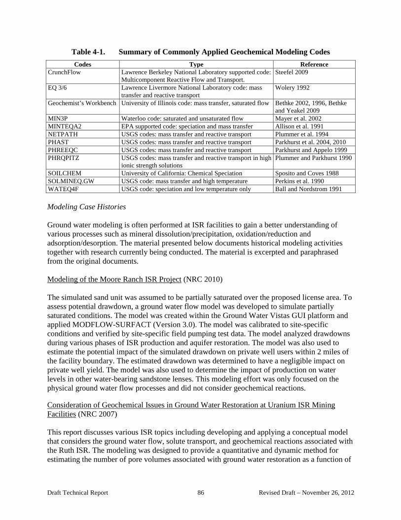
Table 4-1. Summary of Commonly Applied Geochemical Modeling Codes Codes Type Reference
CrunchFlow Lawrence Berkeley National Laboratory supported code: Steefel 2009 Multicomponent Reactive Flow and Transport.
EQ 3/6 Lawrence Livermore National Laboratory code: mass Wolery 1992 transfer and reactive transport
Geochemist’s Workbench University of Illinois code: mass transfer, saturated flow Bethke 2002, 1996, Bethke and Yeakel 2009
MIN3P Waterloo code: saturated and unsaturated flow Mayer et al. 2002 MINTEQA2 EPA supported code: speciation and mass transfer Allison et al. 1991 NETPATH USGS codes: mass transfer and reactive transport Plummer et al. 1994 PHAST USGS codes: mass transfer and reactive transport Parkhurst et al. 2004, 2010 PHREEQC USGS codes: mass transfer and reactive transport Parkhurst and Appelo 1999 PHRQPITZ USGS codes: mass transfer and reactive transport in high Plummer and Parkhurst 1990
ionic strength solutions SOILCHEM University of California: Chemical Speciation Sposito and Coves 1988 SOLMINEQ.GW USGS code: mass transfer and high temperature Perkins et al. 1990 WATEQ4F USGS code: speciation and low temperature only Ball and Nordstrom 1991 Modeling Case Histories Ground water modeling is often performed at ISR facilities to gain a better understanding of various processes such as mineral dissolution/precipitation, oxidation/reduction and adsorption/desorption. The material presented below documents historical modeling activities together with research currently being conducted. The material is excerpted and paraphrased from the original documents. Modeling of the Moore Ranch ISR Project (NRC 2010) The simulated sand unit was assumed to be partially saturated over the proposed license area. To assess potential drawdown, a ground water flow model was developed to simulate partially saturated conditions. The model was created within the Ground Water Vistas GUI platform and applied MODFLOW-SURFACT (Version 3.0). The model was calibrated to site-specific conditions and verified by site-specific field pumping test data. The model analyzed drawdowns during various phases of ISR production and aquifer restoration. The model was also used to estimate the potential impact of the simulated drawdown on private well users within 2 miles of the facility boundary. The estimated drawdown was determined to have a negligible impact on private well yield. The model was also used to determine the impact of production on water levels in other water-bearing sandstone lenses. This modeling effort was only focused on the physical ground water flow processes and did not consider geochemical reactions.
Consideration of Geochemical Issues in Ground Water Restoration at Uranium ISR Mining Facilities (NRC 2007) This report discusses various ISR topics including developing and applying a conceptual model that considers the ground water flow, solute transport, and geochemical reactions associated with the Ruth ISR. The modeling was designed to provide a quantitative and dynamic method for estimating the number of pore volumes associated with ground water restoration as a function of
Draft Technical Report 86 Revised Draft – November 26, 2012

both historical conditions and potential variations (i.e., under different assumptions of future site conditions). Once the conceptual model was developed, the data collected from the site were input into PHREEQC to estimate the number of pore volumes that must be removed to return the system to initial conditions. A series of reactive-transport simulations using ground water restoration data from the Ruth ISR pilot-scale study was used to evaluate variations in the geochemical processes. The calculations showed that a computer code like PHREEQC can be used to make predictive calculations of how different geochemical conditions may affect evolving water quality during geochemical restoration. Irigaray Mine Wellfield Restoration Report, Johnson County, Wyoming (COGEMA 2005) A ground water flow and transport model was developed to assess fate and transport of residual constituents derived from the Irigaray ISR mine. The objective was to demonstrate that residual concentrations would be below regulatory standards at prescribed observation points. The model was used to evaluate continued migration under steady-state conditions, without pumping or injection. Therefore, the emphasis was on adequately representing steady-state advective-dispersive flow within and across the production zone. The approach taken was to develop a model that predominantly depended on advective-dispersive transport of constituents and minimized reliance on geochemical reactions. The parameters required included hydraulic conductivity, hydraulic gradient, dispersivity, and effective porosity. These parameters were quantified for the site and were incorporated into the model. Dispersivity values were based on the scale of the site/plume and literature review. A distribution coefficient (Kd) was included for some constituents using the lowest reasonable Kd available from the literature. Uncertainty was addressed in model parameters with a sensitivity analysis. The codes used to develop the model included:
• MODFLOW: for simulation of the flow field. • MODPATH: for simulation of ground water flow paths. • MT3DMS: for simulation of transport of site-derived constituents.
Although MT3DMS was calibrated to simulate migration of selenium, manganese, uranium, Ra-226, and TDS, it uses the simplified distribution coefficient approach to calculate retardation factors as described in Section 4.7.3. The modeling results demonstrated that remaining concentrations at distances 400 feet down gradient of the wellfield were below the regulatory standards for all the constituents. Ross ISR Project, NRC License Application, Crook County, Wyoming (Strata Energy 2010, Addendum 2.7H Ground Water Model)
The model was developed to analyze the potential direct, indirect, and cumulative hydrological effects of the project on both regional and individual wellfields. As stated in the document, the primary goals of the regional ground water model were to (1) identify potential impacts (if any) to adjacent water rights, (2) estimate long-term impacts from ISR operation, and (3) identify
Draft Technical Report 87 Revised Draft – November 26, 2012

potential impacts to the surficial aquifer and surface impoundments. Modeling goals for individual wellfields were to:
• Estimate adequate perimeter monitoring well offset/setback distances for the wellfield.
• Demonstrate the ability to identify and remedy a lateral excursion (i.e., lixiviants moving past the monitor wells).
• Optimize the wellfield design and pumping rates including bleed rate.
• Evaluate restoration time/efficiency. The hydrogeology of the area ground water use was presented as a basis for the model. The numerical ground water model was the USGS modular finite-difference model MODFLOW and Ground Water Vistas was used as the pre- and post-processor. These codes were selected because of their wide use and acceptance by the industry and regulators. Hydraulic parameters used in the model were based on site data or taken from the literature. The model was first calibrated to a steady-state solution based on pre-1980 conditions. Once a satisfactory calibration to steady-state conditions was achieved, a transient calibration was conducted with the goal of matching the drawdown that had occurred over 30 years due to withdrawals from industrial wells. To assist in the calibration, PEST (a model independent parameter estimation program) was used. The calibrated model was used to simulate ISR operations within the Ross Project area. The ISR simulation was a generalized scenario based on current mapped mineralization. Impacts were also determined along with recovery simulation and flare evaluation. The general conclusion from the modeling was that impacts of the facility would be minor. Lastly, the model is expected to be a useful tool for the final wellfield planning and operations and assist in balancing wellfields, progression planning, and bleed rate optimization. Wellfield Restoration Report, Christensen Ranch Project, Wyoming (COGEMA 2008a) While this report presents a transport assessment:
… no groundwater modeling specific to the Christensen Ranch MUs is included in this report. Christensen Ranch site conditions, including the constituents of concern, are similar to those at the Irigaray Mine. Groundwater modeling included in the Irigaray Mine Aquifer Restoration Report (COGEMA 2003) is referenced where applicable to the Christensen Ranch Site.
The transport assessment comprised the geochemical assessment and hydrological assessment. The geochemical component of the transport assessment addressed the physical and chemical behavior of constituents of concern under the prevailing environmental conditions at the site. These included uranium, radium, iron, manganese, selenium, and sulfate. In addition to the geochemical assessment, the effects of long-term ground water flow, including advective mixing and dispersion, on constituent concentrations were considered under the transport assessment. Direction and velocity of ground water flow are critical hydrologic factors with respect to solute
Draft Technical Report 88 Revised Draft – November 26, 2012

transport. Determination of the direction of ground water flow was based on water-level data that were routinely collected from the monitor well networks.
As previously stated, no ground water modeling was performed specifically for the Christensen Ranch site. However, extensive modeling of ground water flow and solute transport was performed for the Irigaray Mine site located 6 to 10 miles northwest of Christensen Ranch. The Irigaray Aquifer Restoration Report includes those modeling results, which were accepted by the Wyoming Department of Environmental Quality (WDEQ) and NRC. These results apply in a general sense to Christensen Ranch.
The model focused on the impacts of advective mixing on constituent concentrations migrating from the Irigaray site, but did not address the effects of geochemical processes along the flow path. The results of the model indicate that the maximum concentration at a distance of 400 feet from the wellfield was approximately 7 times lower than the initial average wellfield concentration, after subtracting the average background concentration. The background concentration was subtracted from the affected concentrations to normalize the data. The monitor well ring is located 400 feet from the wellfield. Highland Uranium Project A-Wellfield The operator used modeling to show that natural attenuation processes would reduce ground water contamination to acceptable levels. (See Attachment B for details.) The attenuation modeling involved both ground water flow modeling with MODFLOW and PHREEQC geochemical modeling. The calculations showed that a maximum of 15 years would be required to achieve the full benefits of natural attenuation. To support the modeling results, the operator was required to perform semiannual monitoring of four wells (a “hot spot” well with elevated levels of uranium and selenium, an up gradient well, a down gradient well, and a lateral well) beginning in 2004. At the current time, field measurements indicate that the uranium and selenium concentrations are stable, but not declining, as would be expected from natural attenuation and predicted by the geochemical modeling. International Mine Water Association A review of the meetings of the International Mine Water Association (IMWA) uncovered two relevant publications discussing predictive modeling for ISR facilities (Johnson et al. 2010; Johnson 2011). As observed by Dr. Johnson, this effort is still preliminary. Below is a review of the two papers.
Predictive Modeling Strategies for Operations and Closure at Uranium In-Situ Recovery Mines (Johnson et al. 2010) was presented at the IMWA 2010 symposium, “Mine Water and Innovative Thinking.” In this paper, the authors present a predictive strategy, which will be applied at the IRS facility in Edgemont, South Dakota (the proposed Dewy-Burdock facility in Fall River and Custer Counties). The following describes the steps proposed by Johnson et al. 2010:
Draft Technical Report 89 Revised Draft – November 26, 2012
First, a conceptual model must be established to understand the basic hydrogeologic and geochemical system, based on available data and professional expertise. Such a conceptual model includes information such as groundwater flow direction, boundary conditions, along with current groundwater and solid-phase geochemistry. Second, predictive modeling using numerical reactive transport models can be used to simulate future groundwater conditions (during mining, restoration, and post-restoration). This requires the coupled simulation of groundwater flow and geochemical reactions using such models as PHT3d (Prommer 2002), which simulates groundwater flow using MODFLOW (Harbaugh and others 2000) and geochemistry using PHREEQC (Parkhurst and Appelo 1999). In any reactive transport modeling, input data linking the solid-phase mineralogy to the groundwater quality is very important to understand the rock-water interaction. For predictive modeling purposes, the collection of solid-phase geochemistry before mining is required. For final model calibration, postmining solid-phase geochemistry is optimal. Theoretical reactive transport simulations of uranium ISR mining have been examined (Davis and Curtis 2007 [NRC 2007]); however, field applications have been limited. Third, predictive modeling can be used to evaluate the impact on surrounding groundwater quality under the proposed mine plan design and to evaluate possible design alternatives. Since many uranium ISR-amenable deposits occur within sandstones that are drinking water aquifers outside of the ore zone, protection of groundwater quality is of great importance. Predictive reactive transport modeling provides a tool for evaluating potential impacts on surrounding groundwater quality based on initial mine plans. This is part of the second modeling strategy discussed above, but more importantly, alternate well field design and possible restoration procedures can be evaluated before finalizing any mine operation and closure plans. Fourth, model limitations should be evaluated to provide a reasonable range of prediction uncertainties. This step involves the evaluation of uncertainties in the model input parameters, such as geologic layering (Johnson and Friedel 2009) and water chemistry. For example, the integrity of the confining zone should be evaluated based on any uncertainty in geologic logs and can be tested using multiple geologic conceptual models. In addition, any predictions of long-term contaminant transport should provide adequate prediction uncertainties based on the uncertainties of the input data. Multiple conceptual models provide a range of potential groundwater quality impacts. This provides valuable feedback for the collection of additional data, which can assist in reducing uncertainty in future models.
Reactive Transport Modeling for the Proposed Dewey Burdock Uranium In-Situ Recovery Mine, Edgemont, South Dakota, USA (Johnson 2011) was presented at the IMWA 11th International Mine Water Association Congress, “Mine Water – Managing the Challenges.” This paper
Draft Technical Report 90 Revised Draft – November 26, 2012

provides an initial reactive-transport simulation, which supports a conceptual understanding of uranium roll-front formation, current ground water conditions, mining geochemistry, restoration geochemistry, and long-term ground water quality at a uranium ISR site. As the author states, this is the starting point for additional refinements to improve the model. The reactive-transport modeling discussed in the paper used PHAST (Parkhurst et al. 2010), a relatively simple ground water flow code coupled with PHREEQC (Parkhurst and Appelo 1999), to calculate geochemical conditions at each time step. For this work, generic values were assigned to the ground water flow velocities and mass balances for the solid phase. Site-specific data are expected to be added in the future. Even so, some simulations were conducted to simulate pre-mining conditions. In one simulation, ground water with no dissolved oxygen was transported through the model domain. The result was a solid phase uraninite roll-front associated with pyrite on the solid-phase reduced side; uranium and dissolved oxygen were not found in solution. Uranium in-situ mining was simulated using a leach solution fortified with oxygen and carbon dioxide. The resulting oxidation made uranium soluble, and the carbon dioxide created a complexing agent. A five-spot well pattern was simulated with a center pumping well and four surrounding injection wells. In the ore zone, the result was elevated concentrations of uranium in the ground water where the ore zone was being mined. During the restoration phase, the existing wellfield was used to flush out the mining solutions from the ground water. This process was simulated as water with low dissolved constituent concentrations, but with 50 parts per billion (ppb) residual uranium. In one simulation, oxygen was left in the restoration fluids, and in another simulation, oxygen was kept at zero. At this stage, reductant addition to help precipitate uranium could be simulated, but that simulation was not completed for this paper. As noted, the model will be refined as site-specific data are incorporated. Ongoing Research To assist decisionmaking about ISR design, operations, restoration, closure and monitoring will come from the application of reactive transport models. Many such models are already in use to support the ISR mining and new developments in this field (e.g., PHREEQC, Geochemist’s Workbench®), although there are a few sophisticated codes that allow the reactive transport processes to be coupled to the ground water flow regime, such as PHAST or PHT3D. To further investigate data needs, data collection, model applicability and potential modeling approaches, the EPA has entered into a corporative agreement with the U.S. Geological Survey under a Regional Applied Research Effort (RARE). 4.7.4 Demonstrating Long-term Stability of Restored ISR Wellfields – Long-Term
Monitoring and Geochemical Modeling After wellfield restoration efforts have stopped, the restored wellfield is typically monitored for periods of six months to several years, with the intent of demonstrating that the ground water chemistry in the wellfield has reached a “steady state” at compositions as close as possible to the pre-mining background (baseline) levels. While this post-restoration monitoring will provide
Draft Technical Report 91 Revised Draft – November 26, 2012

some confidence that the pre-mining geochemical conditions in the wellfield have returned, the situation may not persist over the long term. The initial injection of chemicals to oxidize and mobilize the uranium ore will most likely also oxidize the chemical reducing agents (electron acceptors) originally present in the aquifer that acted to sequester the uranium in the ore body. These materials are thought to consist of iron sulfide minerals and organic material. If the amounts of these reducing agents have been decreased sufficiently by the mining process, the continual movement of oxidizing waters into the ore zone from up gradient may be too strong for the remnants of the reducing agents to maintain chemically reducing conditions. In that case, the uranium chemically reduced by the restoration process will be re-oxidized and migrate down gradient out of the wellfield over time. In such a situation, the restoration efforts are simply palliative, since they may not restore the underlying mechanism(s) responsible for sequestering the uranium. The long-term prospect is that radionuclides and perhaps toxic metals will move out of the depleted ore zone and into surrounding aquifer areas, because the underlying mechanism for sequestering them has been weakened or totally removed. To detect this possibility, two approaches are possible. In one approach, the post-restoration monitoring could be continued for periods that may be tens of years in duration to detect any deterioration of the chemically reducing conditions in the wellfield, at which point, if detected, remediation efforts could be developed. Such a long monitoring process is necessary, because the kinetics of a re-oxidation process in the field can be slow. Section 7.7.2 examines statistical measures for determining stability in a sequence of measurements considering the influence of natural variability variations and rates of change in the measured parameter. Table 7-20 and Table 7-21 show how many samples (assuming quarterly sampling) are needed to attain high levels of confidence (95% and 99%) that a trend can be detected for various assumed levels of natural variability and parameter change rates. For relatively low natural variability levels and rates of change, the number of samples, and consequently the post-restoration monitoring period, significantly exceed typical post-restoration sampling periods used in practice. A 30-year post-restoration monitoring period proposed in the rulemaking establishes a monitoring period consistent with RCRA regulations. Another alternative is to use geochemical modeling to demonstrate that the restored wellfield and the down gradient geochemical conditions in the exempted aquifer area are sufficient to maintain chemically reducing conditions over the long-term. The modeling used to address the post-restoration possibilities involves relatively simple aqueous speciation modeling, as well as more complex process modeling and perhaps coupled flow and contaminant transport models. As described above, these types of models are readily available and typically used to design the wellfield geometry and optimize production, as well as help design restoration efforts. Their use in assessing post-restoration behavior at an ISR site is discussed further below. The intent of the modeling from a regulatory perspective is to answer two questions:
• Will the ground water chemistry in the restored wellfield keep uranium and other mobilized toxic metals in place?
• Does the down gradient portion of the exempted aquifer have the reducing capacity to remove uranium from ground waters that migrate into the area from the up gradient wellfield area?
Draft Technical Report 92 Revised Draft – November 26, 2012

As a first step in geochemical modeling, it is important to assess the chemical reducing capacity of the ore zone and down gradient portion of the exempted aquifer before the mining is initiated and after the restoration efforts have ceased. This requires information on the nature and amount of chemical reducing agents present in the ore zone before and after the ISR process, as well as down gradient of the ore zone in the remainder of the exempted aquifer area. Concentrations of pyrite (and other iron sulfide minerals) and organic material, as well as other electron acceptor species in the ore zone, should be measured before ISR operations begin and after restoration efforts end. Aqueous indicators of chemically reducing conditions (such as various redox sensitive couples, e.g., sulfide/sulfate, ferric/ferrous iron, redox state measurements, other oxidizing agents such as dissolved oxygen, and nitrate levels) should also be measured in the ground waters. Information on solid-phase electron acceptors can be gathered from analyses of cores taken within the exempted aquifer before operations begin and after restoration efforts stop. Section three of this document contains tabulations of aqueous species that should be monitored for geochemical modeling applications. With the information on concentrations of chemically reducing agents in the ground water and solids within the wellfield and in the down gradient portion of the exempted aquifer, mass balance calculations and process modeling exercises can be done to determine if the reducing capacity of the restored wellfield and down gradient area is sufficient to keep the uranium remaining after the mining in a reduced state, minimizing the potential for migration. While such modeling evaluates the potential for maintaining chemically reducing conditions, kinetic data would allow more sophisticated modeling of reaction progress within the exempted aquifer, including coupling of reaction path and ground water flow modeling. This modeling would examine the reaction rates and evolution of changes in aqueous chemistry as ground waters bearing oxygen and uranium (VI) enter the wellfield area from the up gradient direction, interact with the “restored” wellfield chemistry and move down gradient into the un-mined portion of the exempted aquifer and eventually into the non-exempt portion of the aquifer. Kinetic data to support such modeling is limited (largely to laboratory data with limited field data), but the research described above should significantly increase the field database and understanding of these processes. With sufficiently robust geochemical modeling demonstrating that the system can maintain chemically reducing conditions over the long-term and contain any uranium migrating out of the restored wellfield area within the down gradient portion of the exempted aquifer, the appropriate regulatory authorities may allow a shorter than 30-year post-restoration modeling period. This modeling demonstration is also important for regulatory decisions about the need for alternative concentration levels and the protection of ground water resources in the down gradient area outside the boundary of the exempted aquifer.
Draft Technical Report 93 Revised Draft – November 26, 2012
5.0 ACTIVE/EXISTING ISR FACILITIES: MONITORING ISSUES The standards in 40 CFR 192.32 refer to several sections of RCRA 40 CFR Part 264, Subpart F, which describe EPA’s regulatory approach for releases to ground water from waste management units that store, treat, and dispose of hazardous waste. Although §264.97 is not specifically cited in §192.32, it provides some useful guidance regarding general requirements that could be considered for establishing a suitable ground water baseline:
(g) In detection monitoring or where appropriate in compliance monitoring, data on each hazardous constituent specified in the permit will be collected from background wells and wells at the compliance point(s). The number and kinds of samples collected to establish background shall be appropriate for the form of statistical test employed, following generally accepted statistical principles. The sample size shall be as large as necessary to ensure with reasonable confidence that a contaminant release to ground water from a facility will be detected. The owner or operator will determine an appropriate sampling procedure and interval for each hazardous constituent listed in the facility permit which shall be specified in the unit permit upon approval by the Regional Administrator. This sampling procedure shall be:
(1) A sequence of at least four samples, taken at an interval that assures, to the greatest extent technically feasible, that an independent sample is obtained, by reference to the uppermost aquifer’s effective porosity, hydraulic conductivity, and hydraulic gradient, and the fate and transport characteristics of the potential contaminants, or (2) An alternate sampling procedure proposed by the owner or operator and approved by the Regional Administrator.
In practice, the procedures for establishing the ground water baseline are site specific and are included in the facility license issued by the NRC or Agreement State.
5.1 Ground Water Baseline: Case Studies The requirements for baseline monitoring vary from state to state. (See Section 3.5 for additional details.) In Texas, 26 chemical constituents are measured before mining to establish a baseline, as shown in Table 5-1. This is example data from Production Authorization Area (PAA) No. 1 at the Zamzow ISR facility. Baseline values represent the highest average concentration from either the production or mine area, and are commonly selected as initial restoration goals (Hall 2009). In Table 5-1, the mine area is defined by a line through a ring of monitor wells in the production zone and the production area is defined by a line generally through the outer perimeter of injection and recovery wells.10 TCEQ regulations require a minimum of five baseline wells or
Draft Technical Report 94 Revised Draft – November 26, 2012
10 TCEQ Chapter 331, Subchapter A, §331.2.

one well per four acres, whichever is greater (TCEQ Title 30, Rule §331.104). Sampling frequency and number of samples are not specified by the TCEQ regulations. Uranium Energy Corporation filed a production area authorization (PAA-1) application for the Goliad Uranium Project with the TCEQ on August 27, 2008, and this application was amended on March 27, 2009, to include data from additional baseline wells (Sass 2011). The amended application included 18 baseline wells from the 36-acre production area (i.e., 0.5 wells/acre). The average uranium content for these 18 wells was used to establish a baseline uranium value of 0.115 mg/L. The initial sampling of the 18 wells was conducted over a period of about 11 months (4 wells about July 2007, 6 wells in April 2008, and 8 wells in July 2008). The amended PAA-1 application did not include data from subsequent sampling of all 18 wells in July 2009 and again in November 2009. The averaged uranium assay results for these subsequent periods were 0.029 mg/L and 0.005 mg/L, suggesting that the initial samples were not indicative of geochemical equilibrium. Had the full time series of samples been included in the PAA-1 application, a more rigorous baseline standard would have been set against which to measure restoration.
Table 5-1. Baseline Water Quality Data for Zamzow PAA-1
Parameter Unit Production Zone
Mine Area** Production Area Low Average High Low Average High
1 Cadmium mg/l 122 317 552 195 269 390 2 Magnesium mg/l 15 38.4 84.2 3.0 21.1 40 3 Sodium mg/l 239 387 750 235 383 466 4 Potassium mg/l 19 30.3 49 18.9 26.7 90 5 Carbonate mg/l 0 0 0 0 0 0 6 Bicarbonate mg/l 128 297 400 157 269 346 7 Sulfate mg/l 454 793 1,520 441 601 940 8 Chloride mg/l 350 503 936 394 538 662 9 Fluoride mg/l 0.16 0.54 1.19 0.01 0.36 0.50
10 Nitrate – N mg/l <0.01 0.16 0.9 <0.01 0.14 0.49 11 Silica mg/l 31 51.6 85 11 43.9 74 12 pH Std. units 6.6 7.0 7.66 6.68 7.0 7.45 13 TDS mg/l 1,697 2,289 3,220 1,810 2,037 2,360 14 Conductivity µmhos 2,720 3,204 4,300 2,680 3,049 3,430 15 Alkalinity Std. units 105 275 400 206 238 204 16 Arsenic mg/l <0.001 0.009 0.03 <0.001 0.006 0.044 17 Cadmium mg/l <0.0001 0.001 0.007 <0.0004 0.001 0.0013 18 Iron mg/l 0.01 0.915 8.0 0.03 0.075 0.26 19 Lead mg/l <0.001 0.001 0.006 <0.001 0.004 0.02 20 Manganese mg/l 0.009 0.224 0.82 0.01 0.118 0.19 21 Mercury mg/l <0.0001 0.0004 0.0018 0.0001 0.0006 0.001 22 Selenium mg/l <0.001 0.01 0.01 <0.001 0.004 0.01 23 Ammonia mg/l <0.01 0.374 1.4 <0.01 0.298 0.78 24 Uranium mg/l <0.001 0.171 1.7 <0.001 0.039 0.432 25 Molybdenum mg/l <0.001 0.03 0.95 <0.001 0.226 2.1 26
Radium-226 pCi/l 1.5 155 959 6.5 152 744 ** Monitor wells Source: Hall 2009
Draft Technical Report 95 Revised Draft – November 26, 2012
In its license application for the Moore Ranch Uranium Project in Campbell County, Wyoming, Energy Metals Corporation (2007) proposed to establish the wellfield baseline by sampling production zone wells four times, with a minimum of 2 weeks between samplings (NRC 2010, Section 6.3.1.1). Energy Metals also proposed to sample one well for each 3 acres of mine unit. Data for each sampled parameter would be averaged and used to calculate restoration goals. The average and range of baseline values in the production zone would then be used to assess the effectiveness of subsequent ground water restoration. In another example, at Mine Unit 4 of the Christensen Ranch Project in Wyoming, the wellfield covered about 12 acres and, consequently, 12 injection or production wells were used to establish baseline ground water conditions within the ore zone, which in turn set the restoration goals (COGEMA 1994). The number of baseline wells was based on NRC guidance in NUREG-1569 (NRC 2003, p. 5-39) of one well per acre. Commercial-scale uranium ISR facilities usually have more than one wellfield. For example, the Crow Butte facility in Dawes County, Nebraska, has constructed 10 wellfields since 1991 (Crow Butte 2007). The locations and boundaries for each wellfield are adjusted as more detailed data on the subsurface stratigraphy and distribution of uranium mineralization are collected during wellfield construction. 5.2 Wellfield Restoration Wellfield restoration is defined as those actions taken to ensure that the uranium extraction process will not adversely affect the quality of the ground water adjacent to the ISR wellfields (NRC 2001). This requires returning the wellfield water quality parameters to meet the restoration goals included in the facility license issued by NRC or the Agreement State. Based on pre-mining monitoring, the operator establishes baseline values for the ground water quality. The regulator then uses these baseline values to set restoration goals in the wellfield license. The portion of the aquifer undergoing uranium extraction is exempt from EPA regulatory protection under the SDWA (specifically the UIC Program at 40 CFR Part 144). However, ground water adjacent to the exempted portion of the aquifer must still be protected, and ground water protection provisions for this water are in effect. Similar to the NRC Agreement State provisions,11 an EPA Primacy State may impose more stringent requirements for ground water restoration than the federal program (NRC 2003). Ground water restoration requirements may vary from state to state. Of particular importance is underground injection and point source discharge into surface waters. Currently, UIC programs are administered (as authorized by EPA) in Wyoming, Nebraska, and New Mexico. South Dakota administers the program jointly with EPA. It should be noted that UMTRCA gives NRC the authority to require licensees to restore ground water in the mined aquifer, and EPA to set the standards for that restoration. UMTRCA
11 Texas, Colorado, and Utah operate as Agreement States under NRC regulations in establishing state-specific ISL regulations, while facilities in Wyoming, New Mexico, and South Dakota are directly regulated by NRC. Nebraska is also an Agreement State, but since it does not have specific ISL regulations, its facilities are regulated by NRC.
Draft Technical Report 96 Revised Draft – November 26, 2012

operates separately from SDWA UIC rules, and requires restoration of the ground water in the mined aquifer, even though the water may not be considered potable under SDWA. EPA’s UIC regulations provide protections for non-exempt portions of the aquifer, but generally do not require restoration of the exempt portion unless it may affect drinking water outside its boundaries. State rules under UIC delegation are generally weaker than EPA’s and NRC’s UMTRCA requirements. 5.3 Wellfield Restoration: Case Study
Table 5-2 summarizes restoration results from 22 PAAs in Texas (Hall 2009). It is apparent that, for all of the PAAs, post-restoration analyses exceeded the baseline for some of the parameters tested. Similar information on restoration of sites in other states was extracted from NRC 2009 and is included as Attachment C. Table 5-2 also shows that all of the post-restoration parameters exceeded the baseline in some wellfields. This illustrates the difficulty of restoring wellfields to baseline conditions. However, for most of the species with quantitative limits set by MCLs or secondary drinking water standards, the quantitative limits were below the baseline. Exceptions were fluoride, nitrate, and sulfate where the baseline limits were below recommended standards for all 22 PAAs.
Draft Technical Report 97 Revised Draft – November 26, 2012

Table 5-2. Ground Water Chemistry of Texas In-Situ Uranium Production Authorization Areas
Analyte
EPA and TCEQ Drinking Water
Standards (mg/l)
Baseline Range Post-restoration Range
PAAs with Baseline Above
MCL or Recommended
Standards
PAAs with Post-restoration
Water Above MCL or
Recommended Standards
PAAs Where Post-
restoration Analyses Exceed
Baseline
PAAs Where Post-
restoration Analyses are
Below Baseline
EPA and TCEQ Primary Maximum Contaminant Levels (MCLs): Arsenic 0.01 .004–0.23 .002–.323 77% 55% 18% 82% Cadmium 0.005 0.0001–0.0126 0.0001–0.01 45% 23% 27% 73% Fluoride 4 0.21–1.8 0.29–1.6 0% 0% 31% 69% Lead 0.02 0.003–1.97 0.001–0.05 81% 18% 9% 91% Mercury 0.002 0.0001–0.445 0.0001–0.01 9% 0% 22% 64% Nitrate 10 0.031–10.0 0.001–2.8 0% 0% 4% 96% Selenium 0.05 0.001–0.049 0.001–0.102 18% 4% 54% 45% Radium (226 and 228 Ra: pCi/l) 5 pCi/l 9.36–429.8 5.2–149 100% 100% 4% 96%
Uranium 0.03 0.025–2.0 0.013–3.02 95% 86% 68% 32% TCEQ Secondary Recommended Standards: Sulfate 300 15.8–250 78–3881 0% 18% 86% 14% Chloride 300 196.9–3505 138–3326 86% 86% 22% 78% Total Dissolved Solids 1000 785.7–6349 706.3–6155 81% 77% 31% 55%
Iron 0.3 0.04–5.49 0.01–2.7 54% 9% 4% 96% Manganese 0.05 0.01–0.41 0.01–0.84 77% 50% 40% 60% No Established MCL or Secondary Standards Calcium – 4.13–241 14.7–191 77% 23% Magnesium – 0.477–125 2.27–53 72% 28% Sodium – 200–2356 169–2247 31% 65% Potassium – 6.38–101 6.1–70 14% 86% Carbonate – 0.1–17.9 0–14.6 50% 30% Bicarbonate – 160–500 160–500 66% 25% Silica – 16.3–76 13.4–77.6 19% 81% Conductivity (μmhos/cm) – 1310–11160 1429–3697 76% 24%
Alkalinity (as CaCO3) – 134–349 145–408 81% 10%
Molybdenum – 0.01–0.2 0.0001–3.38 42% 54% Ammonia-N
– 0.01–7.49 0.04–120 76% 24% Baseline and post-restoration data were (14), Alkalinity (11), & Carbonate (10)
Source: Hall 2009
available for all 22 PAAs with the exception of Ra, Mo, K, Si, Bicarbonate, Ammonia (21), Conductivity
Draft Technical Report 98 Revised Draft – November 26, 2012
6.0 ISSUES ASSOCIATED WITH ESTABLISHMENT OF POST-RESTORATION STEADY STATE
During restoration, the operator monitors progress by periodic sampling of the ground water constituents until steady-state conditions are attained. Establishment of steady state requires that the ground water potentiometric surface be restored, to the extent practicable, to its preleaching status, so that the flow regime is similar to that existing before mining. In addition, constituents in the ground water must be in compliance with restoration goals and remain at those levels for a sufficient period to demonstrate that the results are not trending upwards to higher concentration levels. EPA describes a “steady state” as having the following relevant components (EPA 1992, Chapter 7):
1.a After treatment, the water levels and water flow, and the corresponding variability associated with these parameters (e.g., seasonal patterns), should be essentially the same as for those from comparable periods of time prior to the remediation effort.
or 1.b. In cases where the treatment technology has resulted in permanent changes in the ground water system, such as the placement of slurry wells, the hydrologic conditions may not return to their previous state. Nevertheless, they should achieve a state of stability which is likely to reflect future conditions expected at the site. For this steady state, the residual effects of the treatment will be small compared to seasonal changes.
2. The pollutant levels should have statistical characteristics (e.g., a mean and standard deviation), which will be similar to those of future periods.
The first of these components addresses the general behavior and characteristics of the ground water at the site. The second is more judgmental and requires projection of future contamination, based on available current information. These projections cannot be made with certainty; however, various criteria can be used in determining whether a steady state has been reached. Section 7.8 of this report discusses statistical tests for measuring attainment of steady state. When the regulator is satisfied that steady state has been achieved, the operator is authorized to undertake long-term post-restoration stability monitoring. 6.1 Post-restoration Stability Monitoring Once the operator concludes that restoration has been completed and has obtained concurrence from the regulator(s) that a steady state has been established, post-restoration stability monitoring begins. The purpose of the stability monitoring is to demonstrate that the aquifer conditions established at the end of restoration are sustainable over time. Currently, the duration of stability monitoring is a site-specific period of time established in the license(s). In the past, the license-established restoration period typically has been about 6 months (see case histories in Attachment B). More recently, the trend has been to increase the monitoring period established in the license. In practice, the actual period of stabilization may be several years, based on
Draft Technical Report 99 Revised Draft – November 26, 2012

iterative analyses of additional samples requested by the regulators see Table 6-1). If the sandstone in the aquifer is heterogeneous, extended restoration times may be required to ensure that ground water in slow pathways is addressed.
Table 6-1. Post-restoration and Stability Monitoring Periods
Facility Name State
Projected or Estimated
Restoration Period
Projected or Estimated Post-restoration
Monitoring Period Comment/Reference
Moore Ranch Campbell County, 3.5 years 1 year (quarterly) NUREG-1910 Wellfield 1 Wyoming Supplement 1 Moore Ranch Campbell County, 5.25 years 1 year (quarterly) NUREG-1910 Wellfield 2 Wyoming Supplement 1 Nichols Campbell and Johnson 1 to 5 years 1 year (quarterly) NUREG-1910 Ranch Counties, Wyoming Supplement 2 Lost Creek Sweetwater, Wyoming 2 years 6 months (monthly) NUREG-1910
Supplement 3 Ruth Test Site
Johnson, Wyoming 12 months 12 months Schmidt 1989
6.2 Factors That Affect Time Frames for Post-mining Monitoring This section summarizes the factors that must be understood to determine when the impacted aquifer has reached a steady-state condition. 6.2.1 Fate and Transport Processes The monitored time frame is dependent on mass-balance estimates of how much extraction fluid remains in the aquifer. Monitoring during operations needs to determine a mass balance of the total volume of lixiviant injected into the system and the volume withdrawn. The lixiviant used to extract the uranium can mask baseline constituents and affect reaction kinetics. Knowing how much lixiviant remains in the aquifer will aid in understanding whether some reactants are still in the system, have migrated outside the monitored area, or have been temporarily sequestered in low-permeability zones, or are undergoing incomplete or slow reactions that may later release constituents. 6.2.1.1 Speciation The environmental chemistry of uranium is largely dictated by its oxidation state (e.g., Fanghänel and Neck 2002). Under ambient oxidizing conditions, the predominant uranium oxidation state is U(VI). Where oxygen is limited, U(IV) may dominate. The metallic form, U(0), does not occur naturally, and is readily oxidized to U(IV) and eventually U(VI), upon exposure to oxidizing conditions. The mechanisms for the oxidation of U(0) and U(IV) to U(VI) are well established (e.g., NRC 2007). It is rare to find other oxidation states of uranium [e.g., U(V) and U(III)] under natural conditions, due to their instability. However, stable U(V) has been found on mica surfaces (Ilton et al. 2004, Ilton et al. 2005, Ilton et al. 2008).
Draft Technical Report 100 Revised Draft – November 26, 2012
In general, the solubility and therefore the mobility of uranium are greatest when it is in the U(VI) state. Complexation of U(VI) by inorganic anions, such as carbonate, fluoride, and phosphate, may enhance the solubility and mobility of this species. When reducing conditions are present, U(IV) is generally immobile and found either as an insoluble oxide (uraninite) or a silicate (coffinite). Under oxidizing conditions and near neutral pHs, U(VI) species dominate aqueous uranium concentrations. These highly soluble species are generally either hydroxy or carbonate complexes of the uranyl (UO2
2+) cation, although elevated concentrations of potential inorganic ligands near the ISR target zone may exert greater influence on U(VI) speciation (e.g., phosphate). A detailed discussion provided by Demuth and Schramke (2006) describes the geochemical processes controlling the fate and transport of uranium, radium, selenium, arsenic, molybdenum, sulfate, iron and manganese. The authors summarize their findings by reiterating the importance of redox conditions on influencing the mobility of uranium, selenium, arsenic, molybdenum, and sulfur. Although these constituents are likely to be more mobile under relatively oxidizing conditions, adsorption and desorption reactions between uranium, selenium, arsenic, and molybdenum with iron oxide surfaces are particularly important controlling reactions, because iron oxides are widespread in the hydrogeologic environment as coatings on other solids. The precipitation of sulfate phases (e.g., barite, celestite, gypsum) is likely to attenuate sulfate and radium-226 by solid solution. Radium-226 is also strongly attenuated by adsorption onto clay minerals. Under oxidizing conditions, iron and manganese tend to form relatively immobile iron oxyhydroxides and manganese oxides. These oxides may provide adsorption sites for many trace metals, such as uranium, arsenic and molybdenum. Under reducing conditions, particularly as sulfate is consumed and the sulfur is converted to sulfide, concentrations of dissolved metals such as molybdenum decrease as solid-phase metal sulfides are formed. Calcium (or other alkaline earth metals, such as magnesium) and inorganic carbon in ground water tend to dominate the aqueous speciation of U(VI) under near neutral pH conditions. The presence of these species is common in many natural ground water systems (Hem 1985), and as noted below, these speciation characteristics also influence the degree to which U(VI) will adsorb onto aquifer solids. Under reducing conditions, U(IV) species, primarily the uranyl cation and its complexes, predominate, but because of the very low solubility of U(IV) minerals, reach maximum concentrations on the order of 10 nanomolar (2.4 micrograms U/L). For all practical purposes, therefore, only U(VI) aqueous species are at sufficient concentrations to be of environmental concern. Chemical reaction kinetic equations or equilibrium thermodynamic equations can be used to describe chemical interactions among dissolved chemical species, the dissolution of immobile solid phases, or the formation and precipitation of new, immobile solid phases. Geochemical modeling is often performed at ISR facilities to gain a better understanding of thermodynamically controlled processes that include mineral dissolution/precipitation, oxidation/reduction, and adsorption/desorption. Most of the available computer codes assume thermodynamic equilibrium and do not have a method of calculating reaction rates (i.e., kinetics). If a mineral forms or dissolves slowly in a system, the model developed from these codes will not account for these kinetic effects. This is
Draft Technical Report 101 Revised Draft – November 26, 2012
not a major limitation for most aquifer systems, where residence times are measured in years; however, kinetic effects can become more important in modeling reactions anticipated to occur during applied remediation methods, such as the injection of reactants into an aquifer. Ground water flow rates in aquifers undergoing ISR are typically slow, on the order of feet to tens of feet per year, suggesting that the development of geochemical models for these environments may not be severly limited due to a lack of site-specific knowledge of kinetic effects for chemical reactions that occur during and after restoration efforts. 6.2.1.2 Speciation: Case Study The experience with iron at the Crow Butte ISR facility is illustrative of speciation problems. Crow Butte Resources (CBR) experienced difficulty in reaching desired iron levels during wellfield restoration. During the initial stabilization monitoring period in 1999, the iron concentration averaged 0.089 mg/L. Subsequent testing in the summer of 2002 showed an average iron content of 0.278 mg/L. The operator attributed this to speciation initiated by the original injection of lixiviant, with subsequent transitory solubility increases resulting from the selected restoration method. As CBR stated (Crow Butte 2002):
CBR believes that the elevated iron concentrations are due to the restoration process and will ultimately decrease to concentrations well below the restoration standard. During the in situ mining process, when the groundwater is oxygenated and the Eh is positive, the iron contained in pyrites is oxidized to ferric iron and forms ferric oxyhydroxides. The ferric oxyhydroxides are extremely insoluble, which explains the very low concentrations of iron in solution during mining, indicated by the end of mining values which, with the exception of one restoration well (PR-19), were below the detection limit of 0.05 mg/L. During the active restoration process, however, sodium sulfide is used as a reductant to decrease the Eh of the groundwater. As the Eh drops, the stable solid iron phase is reduced from ferric iron to ferrous iron, which is more soluble. During the transition from ferric to ferrous iron, the iron concentration in the groundwater increases significantly. This increase in the iron concentration is transitory and, as the Eh continues to decrease, iron sulfide minerals will be the dominant iron phase. Because of the relative insolubility of these iron sulfide minerals, this will cause a significant decrease in the iron concentration in solution. Based on these mechanisms, CBR expects that the elevated concentrations of iron at the current time will ultimately decrease.
Without greater insight into the mineralogy and flow and transport processes within the aquifer, however, there is no reliable means to test CBR’s hypothesis. Active research is being conducted to better understand the processes controlling aquifer restoration. For example, Cameco Resources is currently seeking permission from the Wyoming Department of Environmental Quality to conduct a series of aquifer restoration experiments at Smith Ranch mine, which include: (1) tracer tests to determine the hydrologic pathways between injector and recovery wells; (2) bio-stimulation tests to determine the viability of using naturally occurring bacteria to re-precipitate uranium and other redox-sensitive species; and (3) natural attenuation tests to
Draft Technical Report 102 Revised Draft – November 26, 2012
determine the ability of the aquifer down gradient of the mining zone to immobilize contaminants (Cameco 2012). 6.2.1.3 Solubility Under most natural conditions, the thermodynamically stable uranium solid phases will be either U(VI) or U(IV) compounds. The most stable U(VI) compounds are the phosphates and vanadates, but their formation is often limited by the relatively low concentrations of these two anions, and thus more soluble U(VI) oxides, such as schoepite, are often seen if any U(VI) solid phases are present. A significant fraction of the solid-phase U(VI) will be adsorbed to iron (hydr)oxide surfaces, to the edges of clay minerals, and to organic matter, rather than precipitated as discrete uranium phases. Maximum solubility of uranium is seen in oxidizing, phosphate-free, carbonate-rich solutions, and consequently, carbonates (or bicarbonates) and oxygen or hydrogen peroxide are the principal reagents used for ISR mining. Under reducing conditions, the stable U(IV) solid phases are uraninite and, if high amounts of dissolved silica are present, coffinite. Organic complexes of U(IV) associated with humic material may also retain U(IV) in the solid phase. The solubility of the U(IV) phases is extremely low, and thus the presence of reducing conditions effectively halts or slows the movement of uranium in soils and sediments, provided that colloidal-sized uranium-bearing particles are not formed and transported. The most common uranium ore-forming process involves reductive precipitation of U(IV) phases as a result of microbiological activity to form a roll-front deposit (Langmuir 1997). The stability fields for U(VI) and U(IV) as a function of pH and Eh for various water compositions suggest that a wide variety of uranium-bearing precipitates are possible, especially in complex ground water systems that invariably contain silica, carbonate/bicarbonate, calcium/magnesium, sodium, and sometimes phosphate. Furthermore, it may be difficult to predict associations of uranium in the solid phase based on analysis of aqueous chemical data and solubility predictions from thermodynamic chemical data. In the absence of confirmatory solid-phase characterization data, equilibrium model projections indicate only the possible formation of specific uranium-bearing precipitates. 6.2.2 Natural Attenuation Processes Natural attenuation processes include a variety of physical, chemical, and biological processes that can act to reduce the mass, mobility, volume, or concentration of contaminants in ground water. Attenuation processes important at ISR sites include pH buffering and acid neutralization, adsorption at the mineral-water interface, mineral precipitation, and dilution/dispersion. 6.2.2.1 Adsorption Adsorption processes are typically categorized by the relative “strength” of the interaction between the adsorbate (species in solution) and the surface or adsorbent. If water molecules are positioned between the cation or anion and the surface, the adsorption complex is referred to as outer sphere and is considered to be weak. Conversely, if upon adsorption, the adsorbate loses waters of hydration such that no water molecules are positioned between the cation or anion and the surface, the adsorption complex is referred to as inner sphere and is considered to be strong.
Draft Technical Report 103 Revised Draft – November 26, 2012

Adsorption of uranium typically involves inner-sphere complexation of uranyl (i.e., UO2
2+) species by oxygen ligands at the surfaces of iron oxyhydroxides, phosphates, and layered silicates. Uranyl species exhibit a high affinity for iron oxyhydroxide surfaces and for both basal and edge sites on layered aluminosilicates, such as the clays smectite and vermiculite. Adsorption of U(VI) to the aluminosilicate mineral, muscovite, has been observed in aquifer sediments at the Hanford Site in Richland, Washington (McKinley et al. 2007). Complexation of U(VI) by organic ligands in solid humic materials (primarily carboxylic-acid and phenolic groups) may also serve to remove uranium in shallow ground water systems (Sowder et al. 2003). A compilation of published Kd values for U(VI) sorption onto soils/sediments is documented in EPA 1999a. However, the authors of that compilation recognized that there are major limitations to the application of published Kds for site-specific applications where either the ground water chemistry or the aquifer matrix differs significantly from the conditions under which a Kd was determined (Ochs et al. 2006). One interesting study examined uranium sorption in a sandstone aquifer under site-specific conditions by back-calculating a Kd for the observed uranium distribution after developing a validated ground water flow model for the aquifer using flow rates and carbon isotope data for the ground water system (Pearson et al. 1983). Areas of chemically oxidizing and reducing conditions in the aquifer were observed, indicating that uranium reduction processes were active similar to those involved in the formation of roll-front deposits. A Kd of 6 was proposed for uranium sorpion on the ssandstones based on the field data and validated hydrologic model. Most of the information on uranium sorption reported in the literature is derived from laboratory measurements, in contrast to the the study referenced above. Davis et al. (2004) document a Surface Complexation Model (SCM) alternative to the constant K approach. As described by Davis et al. (2004), there are two major methods for applying the SCM concept; the Component Activity (CA) and the Generalized Composite (GC) approaches. In the CA approach, it is assumed that a mineral assemblage is composed of a mixture of one or more reference phases, whose surface chemical reactions are known from independent studies of each phase. Next, based on a measurement of the relative amounts or surface areas of each mineral present in the soil or sediment, adsorption by the mixture of phases can be predicted by an equilibrium calculation, without any fitting of experimental data for the mixture. In the GC approach, the surface of the mineral assemblage is considered too complex to be quantified in terms of the contributions of individual phases to adsorption. In the GC approach, it is assumed that adsorption can be described by mass laws written with “generic” surface functional groups, with the stoichiometry and formation constants for each mass law determined by fitting experimental data for the mineral assemblage as a whole.
This SCM approach incorporates the important influence of uranium solution speciation, while avoiding the need to model the influence of individual mineral components (and their respective surface charging behavior). While this approach still requires site-specific data, it provides a means for projecting the influence of changes in ground water chemistry on uranium sorption. The chemistry of ground water may be influenced by reaction with aquifer solids and/or external recharge/infiltration from atmospheric precipitation or surface water. As previously noted, alkalinity influences the aqueous speciation of U(VI), and it also influences the degree of sorption of U(VI) onto iron oxyhydroxides and aquifer solids in which these minerals control
Draft Technical Report 104 Revised Draft – November 26, 2012

uranium partitioning (e.g., Um et al. 2007). It has been demonstrated that changes in ground water chemistry influence the transport of U(VI) through an aquifer (Yabusaki et al. 2008). Alternatively, transition from oxidizing to reducing conditions along the transport pathway may be accompanied by a shift from adsorption of U(VI) species to precipitation of U(IV)-bearing solids (Davis et al. 2006). Reactive-transport models used to project subsurface uranium mobility directly incorporate the influence of major ion chemistry and redox conditions on the chemical speciation of uranium.
Field evidence shows that adsorption of uranium to mineral surfaces within an aquifer may be an intermediate step to the formation of uranium-bearing precipitates. Murakami et al. (2005) have observed the association of nanoparticulate U(VI)-phosphate precipitates with iron oxyhydroxides in the weathering zone down gradient from a uranium ore deposit. The U(VI) mineral was identified as metatorbernite, which was present in ground water that was undersaturated with respect to precipitation of this mineral. Characterization of the textural associations between the nanocrystalline metatorbernite and iron oxyhydroxides present as fissure fillings, clay coatings, and nodules, along with compositional relationships between copper, phosphorus, and uranium (Sato et al. 1997), indicated that the formation of uranium precipitates was a secondary step following initial adsorption of these constituents onto iron oxyhydroxide mineral surfaces (Murakami et al. 2005). As summarized by Payne and Airey (2006), the observations in this subsurface system provide a point of reference for designing site characterization strategies and developing both conceptual and analytical models for interpreting and projecting uranium mobility in ground water. O’Loughlin et al. (2003) believe that mixed ferrous/ferric hydroxides (i.e., green rust) play a central role in the biogeochemistry of iron. The authors conclude that their experimental results clearly indicate that U(VI) (as the soluble uranyl ion) is readily reduced by green rust to U(IV) in the form of relatively insoluble UO2 nanoparticles, suggesting that the presence of green rusts in the subsurface may have significant effects on the mobility of uranium, particularly under iron-reducing conditions. Lee et al. (2010) found that biogenic UO2 (uraninite) nanocrystals may be formed as a product of a microbial reduction process in uranium-rich environments. These results will extend the limited knowledge of microbial uraniferous mineralization and may provide new insights into the fate of aqueous uranium complexes. 6.2.2.2 Role of Secondary Minerals The oxidation of iron sulfides in the host rock results in the release of iron, sulfate, acidity, and metals to solution. High aluminum and silica concentrations are also commonly encountered in mine effluents and are the result of weathering of aluminosilicate minerals at low pH. Oxidation and hydrolysis reactions can subsequently lead to the precipitation of a wide array of hydroxide, sulfate, and/or hydroxysulfate minerals, depending on geochemical and biogeochemical conditions (Nordstrom and Alpers 1999). These secondary minerals play important roles in attenuating contaminants in the ground water. Secondary precipitates can remove contaminants from affected waters through adsorption and/or coprecipitation reactions. The extent to which dissolved contaminants will sorb onto secondary precipitates as outer sphere or inner sphere complexes will vary as a function of the contaminant
Draft Technical Report 105 Revised Draft – November 26, 2012
species, the secondary precipitate, pH, particle size and surface area, and the presence of other sorbing species that may compete for adsorption sites. Inorganic contaminants may be removed from solution due to precipitation of an insoluble phase in which the contaminant represents a major or minor component within the solid. Examples of secondary precipitates that form in impacted sites include oxyhydroxides [e.g., FeOOH(s)], hydroxysulfates [e.g., Fe8O8(OH)6(SO4)(s)], sulfates [e.g., PbSO4(s)], and sulfides [e.g., ZnS(s)]. For each of these minerals, there will be a limited compositional range of ground water chemistry over which precipitation could occur, and formation of these precipitates may compete with other removal processes, such as adsorption. The potential for contaminant precipitation can be estimated by evaluating the saturation state of the ground water with respect to possible precipitate phases using a saturation-state modeling approach. To evaluate whether ground water is oversaturated, undersaturated, or at equilibrium with a particular phase, computer geochemical speciation models are of practical use. As an example, consider the solubility expression for lead sulfate (anglesite). The mass-action expression that applies to the equilibrium is:
PbSO4(s) = Pb2+ + SO42-
A natural water may or may not be at saturation with respect to anglesite, depending on whether the phase is actually present, available surface area, residence time of water, and kinetic factors that may impede dissolution and/or precipitation. If equilibrium is assumed between water and anglesite, then the ion activity product, Q, should be the same as the equilibrium constant, Kr:
where the activity, a, of PbSO4(s) is taken to be 1. Because ion activity products may vary by orders of magnitude, it is often more convenient to take the logarithm of the ratio; that is, to compute the saturation index, SI:
where SI = 0 at equilibrium. If the water is oversaturated in a particular phase, then the SI is positive, and there is a thermodynamic driving force for precipitation to occur. If the water is undersaturated, then the SI is negative, and the mineral, if present, will tend to dissolve:
SI > 0 if oversaturated and
SI < 0 if undersaturated
Draft Technical Report 106 Revised Draft – November 26, 2012

As previously indicated, the ground water chemistry will dictate the stability of a precipitate. Contaminant remobilization will occur as a result of dissolution of the precipitate phase, for example, when log Q/Kr < 0. Precipitate dissolution may occur due to ground water acidification, oxidation/reduction of precipitate components, dilution, or complexation of the precipitate component(s) with dissolved species that form more stable compounds. A key point is that attenuation processes involving inorganic contaminants are reversible (e.g., Gault et al. 2005; Moncur et al. 2005). Metals taken up at the mineral-water interface can be released back into solution. Geochemical modeling of mineral stability and contaminant adsorption/desorption behavior can provide insight into contaminant remobilization potential due to future changes in geochemical conditions. However, it must be noted that thermodynamic databases are often incomplete, and thermodynamic constants for specific compounds may vary from database to database. Thus, results from geochemical models must be carefully reviewed. In addition, the method outlined above assumes equilibrium conditions and ignores rates (i.e., kinetics) of mineral dissolution and precipitation. However, data are often lacking on the kinetics of biogeochemical processes responsible for contaminant uptake and remobilization, especially data that can be applied in field systems to predict the long-term behavior of contaminants. With respect to predicting geochemical interactions at ISR facilities, several concerns raised by a reviewer of the geochemical modeling of an ISR facility and presented in NUREG-6820 (NRC 2007) illustrate the potential impacts from these types of limitations. The reviewer noted that since the applied model is nonkinetic, any bacterial influences from naturally occurring Desulfovibria and Thiobacillus are eliminated from consideration. The comment also noted that these influences may be as (or more) important to long-term stability than the addition of reductant during restoration. In addition, the role of pyrite during both restoration and stabilization was a concern, and the reviewer noted that a kinetic approach might result in simulations that more closely compared with observed conditions. 6.2.2.3 Role of Biological Processes The purpose of the stabilization phase of aquifer restoration is to establish a chemical environment that reduces the solubility of dissolved constituents, such as uranium, arsenic, and selenium. An important part of stabilization during aquifer restoration is metals reduction (NRC 2007). During uranium recovery, if the oxidized (more soluble) state is allowed to persist after uranium recovery is complete, metals and other constituents such as arsenic, selenium, molybdenum, uranium, and vanadium may continue to leach and remain at elevated levels. To stabilize metals concentrations, the pre-operational oxidation state in the ore production zone should be re-established to the extent possible. This may be achieved by adding an oxygen scavenger or reducing agent, such as hydrogen sulfide (H2S), or through bioremediation (NRC 2007). Bioremediation of uranium contamination has been under field and laboratory investigation since originally proposed in the early 1990s, with most of the efforts occurring in the last 10 to 12-years (see Abdessalem et al. 1999 for a listing of references on the subject). In bioremediation, the added bacteria use organic materials or other electron donor species in the ground water to generate electrons that are then transferred to an electron acceptor [ideally U(VI)] as the end product of the bacterial metabolic process. For bioremediation, bacteria are
Draft Technical Report 107 Revised Draft – November 26, 2012

used in combination with electron donor materials (e.g., acetate or lactate ions) to reduce U(VI) to U(IV) in an effort to immobilize the uranium and prevent its migration away from the initial contaminant source area into surrounding ground waters. Once uranium is chemically reduced, it is anticipated that the uranium will precipitate in the host rock pore space or be adsorbed on the surface of minerals in the host rock and remain sequestered within the treated area. Laboratory studies of bioremediation illustrate that various bacteria and electron donor materials in contact with aqueous U(VI) result in a reduction of uranium (see Long et al. 2008 and Yabusaki et al. 2010 for extensive summaries of these studies). In addition to bioremediation using added organic electron donor species, reduction of U(IV) with nitrate, sulfate, and ferrous iron species added to ground water has been reported (Moon et al. 2009, Jeon et al. 2005). Sulfate-reducing bacteria have the ability to attenuate the movement of metals through the precipitation of sulfide minerals (e.g., Gammons et al. 2005) and by raising the pH of the water. This process is recognized in the restoration of ISR sites and also occurs in the natural environment (Church et al. 2007). These results have greatly increased interest in using bioremediation techniques and led to some field applications. Most of the field studies testing uranium contamination bioremediation have involved situations somewhat different than those presented for ISR operations. The source of the uranium contamination is the introduction of U(VI) into the subsurface from activities on the surface, such as the disposal of mill tailings or uranium wastes spilled on the ground surface or disposed of by shallow land burial methods. For these situations, U(VI) enters the vadose zone and penetrates to the water table, where it can migrate to contaminate surrounding ground water. In field studies of these situations, the ground water is injected with bacteria and other chemical additives to initiate the uranium reduction and immobilization process. For an ISR site, the uranium is initially present in the subsurface in a chemically reduced state from the mechanisms that originally deposited the ore body. In the ISR process, the reduced uranium is oxidized by chemicals pumped into the ore zone and later reduced by the addition of other chemicals during the aquifer restoration phase, with the expectation that the more mobile U(VI) will precipitate and remain in the wellfield. Bioremediation field studies for the ISR application have not been reported on extensively. While laboratory results for bioremediation of U(VI) contamination were very promising, additional studies and field testing have not met with unqualified success (Charbonneau 2009). Uranium (VI) adsorbed on minerals in the subsurface is significantly less available kinetically for reduction by bacteria (Liu et al. 2009, Ortiz-Bernard et al. 2004). This finding may be particularly relevant to ISR applications, since the oxidizing conditions during operations may result in sorption of U(VI) on the host rock and subsequent resistance of the oxidized uranium to be reduced and stay immobile in the changing chemical environment during and after ground water restoration. Re-oxidation of U(IV) has been observed due to reaction with sulfate, nitrate, and ferric iron during chemical reduction of these species by other bacteria (Moon et al. 2009). For the ISR situation, the introduction of sulfate and ferric iron species to promote chemically reducing conditions, as well as the presence of elevated nitrate levels in some near-surface aquifer systems, may in fact work against the long-term immobilization of uranium in a restored ISR wellfield. During the initial oxidation process, iron sulfide minerals will also be oxidized by the lixiviant and ferric iron remaining in the wellfield ground water during restoration would
Draft Technical Report 108 Revised Draft – November 26, 2012
compete with remaining U(VI) for reduction to iron sulfides again. A study by Wan et al. (2005) showed that the microbially mediated reduction of U(VI) to U(IV) can be transient, even under sustained reducing conditions. These authors found that uranium was reduced during the first 80 days, but after 100 to 500 days, it was re-oxidized and solubilized, even though the microbial community capable of reducing U(VI) was sustained. In addition, the ISR restoration process involves injection and withdrawal of chemicals into the oxidized wellfield under a strong flow gradient. For bioremediation efforts, this relatively rapid flushing of ground water through the wellfield would probably severely limit the effectiveness of bioremediation by simply removing the bacteria before they have opportunity to work effectively. For bioremediation attempts, it may be more productive to “inoculate” a restored wellfield with the appropriate bacteria after the typical restoration efforts are stopped and the pumping in the wellfield ceases. The longer-term monitoring periods proposed in the rulemaking would then allow the progress of a bioremediation step to be monitored over a longer time frame, since only the natural flow of ground waters through the wellfield would affect the bacteria population. The net effect of these processes may result in a slow oxidation of uranium left in a “restored” ISR wellfield over the long-term, supporting the use of a longer post-restoration monitoring period than has been used previously in the industry. Additional field studies involving restored wellfields would allow the mechanisms mentioned above to be assessed to determine their long-term effects under actual field conditions. These studies would be welcomed and may significantly elevate confidence that a “restored” ISR wellfield will remain that way for the long-term. Cameco Resources is considering bio-stimulation tests to determine the viability of naturally occurring bacteria to re-precipitate uranium and other redox sensitive species. Prior studies by Cameco at Smith Ranch showed that a mixture of safflower oil and ethanol or cheese whey alone resulted in rapid reductions of uranium, arsenic, and selenium in the ground water, but these amendments caused pump plugging problems (Cameco 2012). Cameco is proposing additional testing using other organic molecules to promote bio-stimulation. Cameco noted that studies at various DOE sites involved ground water with substantially different geochemistry than that at ISR facilities. In addition, the proposed Smith Ranch studies involved deeper-lying waters that are less susceptible to variations in oxygen contamination than the near-surface waters involved in the DOE studies. 6.3 Geochemically Based Restoration Techniques Another component of aquifer restoration is accomplished by establishing a chemical environment that alters the solubility of dissolved constituents, such as uranium, arsenic, and selenium. These methods typically invoke chemical reactions in which the valence state of elements is either oxidized to a higher valence state or reduced to a lower valence state. During uranium recovery, if the oxidized (more soluble) state is allowed to persist after uranium recovery is complete, metals and other constituents such as arsenic, selenium, molybdenum, uranium, and vanadium may continue to leach and remain at elevated levels. For example, if
Draft Technical Report 109 Revised Draft – November 26, 2012
arsenic concentrations in mildly oxidizing water down gradient from an ISR facility must be lowered, then either increasing the redox potential to precipitate a less soluble arsenic oxide or reducing the redox potential and adding sulfide to form a less soluble sulfide mineral might be considered. Some of the issues to consider in the applied redox approach are the type and amount of reactant, means of emplacement, reaction kinetics, unwanted byproducts, solubility of contaminant-containing minerals, and geochemical stability of the imposed barrier environment. As noted above, another method used to stabilize metals by the re-establishment of their pre-operational oxidation states is to add an oxygen scavenger or reducing agent [such as hydrogen sulfide (H2S)] or a biodegradable organic compound (such as ethanol) into the uranium production zone during the later stages of recirculation (NRC 2007).
As described in the case studies summarized in NRC (2007), sampling at some sites after H2S injection indicated that although reducing conditions were apparently achieved, they were not maintained over the longer term. For example, as a field test of ground water stabilization during aquifer restoration, hydrogen sulfide gas was injected as a reductant into the Ruth ISR research and development facility in Campbell County, Wyoming. After 6 weeks of hydrogen sulfide injection, the pH dropped relatively quickly from 8.6 to 6.3, and the sulfate concentration increased from 28 parts per million to 91 parts per million, indicating that the sulfide reductant was being consumed (NRC 2007). Concentrations of dissolved uranium, selenium, arsenic, and vanadium decreased by at least one order of magnitude. After 1 year of monitoring, however, reducing conditions were not maintained, and uranium, arsenic, and radium concentrations began to increase, suggesting that the amount of hydrogen sulfide injected was not sufficient to fully reduce all the material oxidized during the mining phase. Based on the available field data from aquifer restoration, NRC (2007) concluded that aquifer restoration is complex and results can be influenced by several site-specific hydrological and geochemical characteristics, such as pre-operational baseline water quality, lixiviant chemistry, aquitard thickness and continuity, aquifer mineralogy, porosity, and permeability. In some cases, such as at Bison Basin and Reno Creek, the aquifer was restored in a relatively short time. In other cases, restoration required much more time and treatment than was initially estimated (e.g., the A- and C-Wellfields at the Highland ISR facility). 6.4 Monitored Natural Attenuation MNA refers to the reliance on natural attenuation processes to achieve site-specific remediation objectives within a reasonable time frame. Natural attenuation processes include a variety of physical, chemical, and/or biological processes that act without human intervention to reduce the mass or concentration of contaminants in soil and ground water. These in-situ processes include biodegradation, dispersion, dilution, sorption, and volatilization; radioactive decay; and chemical or biological stabilization, transformation, or destruction of contaminants (EPA 1999a). The overall impact of natural attenuation processes at a given site can be assessed by evaluating the rate at which contaminant concentrations are decreasing either spatially or temporally. Guidelines included in Office of Solid Waste and Emergency Response (OSWER) Directive 9200.4-17P (EPA 1999a) and by the American Society for Testing and Materials (ASTM 1998) have endorsed the use of site-specific attenuation rate constants for evaluating natural attenuation
Draft Technical Report 110 Revised Draft – November 26, 2012

processes in ground water. The EPA directive on the use of MNA at Superfund, RCRA, and underground storage tank sites (EPA 1999a) includes several references to the application of attenuation rates:
Once site characterization data have been collected and a conceptual model developed, the next step is to evaluate the potential efficacy of MNA as a remedial alternative. This involves collection of site-specific data sufficient to estimate with an acceptable level of confidence both the rate of attenuation processes and the anticipated time required to achieve remediation objectives. At a minimum, the monitoring program should be sufficient to enable a determination of the rate(s) of attenuation and how that rate is changing with time.
Site characterization (and monitoring) data are typically used for estimating attenuation rates. The ASTM Standard Guide for Remediation of Ground Water by Natural Attenuation at Petroleum Release Sites (ASTM 1998) also identifies site-specific attenuation rates as a secondary line of evidence of the occurrence and rate of natural attenuation. The 1999 OSWER Directive also provides some general guidelines for use of MNA as a remedial approach for inorganic contaminants (EPA 1999a). The key policy concerns are that the specific mechanisms responsible for attenuation of inorganic contaminants should be known at a particular site, and the stability of the process should be evaluated and shown to be irreversible. The specific policy language is as follows:
MNA may, under certain conditions (e.g., through sorption or oxidation-reduction reactions), effectively reduce the dissolved concentrations and/or toxic forms of inorganic contaminants in groundwater and soil. Both metals and non-metals (including radionuclides) may be attenuated by sorption reactions such as precipitation, adsorption on the surfaces of soil minerals, absorption into the matrix of soil minerals, or partitioning into organic matter. Oxidation-reduction (redox) reactions can transform the valence states of some inorganic contaminants to less soluble and thus less mobile forms (e.g., hexavalent uranium to tetravalent uranium) and/or to less toxic forms (e.g., hexavalent chromium to trivalent chromium). Sorption and redox reactions are the dominant mechanisms responsible for the reduction of mobility, toxicity, or bioavailability of inorganic contaminants. It is necessary to know what specific mechanism (type of sorption or redox reaction) is responsible for the attenuation of inorganics so that the stability of the mechanism can be evaluated. For example, precipitation reactions and absorption into a soil’s solid structure (e.g., cesium into specific clay minerals) are generally stable, whereas surface adsorption (e.g., uranium on iron-oxide minerals) and organic partitioning (complexation reactions) are more reversible. Complexation of metals or radionuclides with carrier (chelating) agents (e.g., trivalent chromium with EDTA) may increase their concentrations in water and thus enhance their mobility. Changes in a contaminant’s concentration, pH, redox potential, and chemical speciation may reduce a contaminant’s stability at a site and release it into the environment. Determining the existence, and demonstrating the irreversibility, of these mechanisms is important to show that a MNA remedy is sufficiently protective.
Draft Technical Report 111 Revised Draft – November 26, 2012
6.4.1 Tiered Approach to Assessing Suitability of Monitored Natural Attenuation EPA’s Office of Research and Development has prepared a technical resource document for the application of MNA to inorganic contaminants in ground water (Reisinger et al. 2005; EPA 2007a and 2007b). The technical resource document presents a four-tiered assessment of MNA as a viable response action for selected metal, metalloid, and radionuclide contaminants encountered in ground water at a particular location. Components of the approach common to each tier include (1) demonstrating contaminant sequestration mechanisms, (2) estimating attenuation rates, (3) estimating attenuation capacity of aquifer solids, and (4) evaluating potential reversibility issues. EPA expects that users of this document will include EPA and state cleanup program managers and their contractors, especially those individuals responsible for evaluating alternative cleanup methods for a given site or facility. A decision-making approach is provided for evaluating MNA as a possible response action for contaminated ground water. Emphasis is placed on developing a more complete understanding of the site through development of a conceptual site model that includes an understanding of the attenuation mechanisms, the geochemical conditions governing these mechanisms, and indicators that can be used to monitor attenuation progress (EPA 2007a). EPA judges this tiered decision-making approach to be an appropriate and cost-effective way to screen out sites unsuitable for MNA, while collecting the most relevant data at sites that might be amenable to this approach. Conceptually, a tiered assessment of MNA seeks to progressively reduce site uncertainty as MNA-specific data are collected. MNA for inorganics and radionuclides is most effectively implemented through four tiers that require progressively more information on which to assess the reasonableness of MNA:
• Tier I. The plume is not threatening public health, is stable, and some direct evidence of contaminant attenuation exists.
• Tier II. The attenuation capacity of the site exceeds the estimated mass of contaminant at the site.
• Tier III. There is strong evidence that attenuation mechanism(s) will prevail over long periods of time.
• Tier IV. A record of decision, including a long-term monitoring plan and other site closure considerations, is developed.
6.4.2 First-Order Attenuation Rate Determination First-order attenuation rate constant calculations are an important consideration for evaluating natural attenuation processes at ground water contamination sites. Specific applications identified in EPA guidelines (EPA 1999a) include use in characterization of plume trends (shrinking, expanding, or showing relatively little change), as well as estimation of the time required to achieve remediation goals. As described by Newell et al. (2002), the use of the attenuation rate data for these purposes is complicated, as different types of first-order rate constants represent very different attenuation processes:
Draft Technical Report 112 Revised Draft – November 26, 2012
Concentration versus time rate constants are used for estimating how quickly remediation goals will be met at a site. In units of inverse time (e.g., per day), they are derived as the slope of the natural log concentration versus time curve measured at a selected monitoring location. Concentration versus distance bulk attenuation rate constants are used for estimating whether a plume is expanding, showing relatively little change, or shrinking because of the combined effects of dispersion, biodegradation, and other attenuation processes. The attenuation rate constant, in units of inverse time (e.g., per day), is derived by plotting the natural log of the concentration versus distance and (if determined to match a first-order pattern) calculating the rate as the product of the slope of the transformed data plot and the ground water seepage velocity contaminant transport versus transport of a tracer, or more commonly, calibration of a solute transport model to field data.
To interpret the past behavior of plumes, and to predict their future behavior, it is necessary to describe the behavior of the plume in both space and time. Therefore, the collection of long-term monitoring data from wells that are distributed throughout the plume is important. Concentration versus time rate constants describe the behavior of the plume at one point in space, while concentration versus distance rate constants describe the behavior of the entire plume at one point in time. Under appropriate conditions, each of these constants can assist in site-specific evaluation and quantification of natural attenuation processes. Each of these terms is identified as an “attenuation rate.” Because the rate constants differ in their purpose and relevance, it is important to understand their proper application, as summarized below.
Concentration versus Time Rate Constants: A rate constant derived from a concentration versus time (C vs. T) plot at a single monitoring location provides information regarding the potential plume longevity at that location, but that information cannot be used to evaluate the distribution of contaminant mass within the ground water system. The C vs. T rate constant at a location within the source zone represents the persistence in source strength over time and can be used to estimate the time required to reach a remediation goal at that particular location. To adequately assess an entire plume, monitoring wells must be available that adequately delineate the entire plume, and an adequate record of monitoring data must be available to calculate a C vs. T plot for each well. At most sites, the rate of attenuation in the source area is slower than the rate of attenuation of materials in ground water, and plumes tend to shrink back towards the source over time. In this circumstance, the life cycle of the plume is controlled by the rate of attenuation of the source and can be predicted by the C vs. T plots in the most contaminated wells. At some sites, however, the rate of attenuation of the source is rapid compared to the rate of attenuation in ground water. This pattern is most common when contaminants are readily soluble in ground water and when contaminants are not biodegraded in ground water. In this case, the rate of attenuation of the source as predicted by a C vs. T plot will underestimate the lifetime of the plume. This behavior would be expected at ISR sites, following the remediation of the source. Concentration versus Distance Rate Constants: Attenuation rate constants derived from concentration versus distance (C vs. D) plots serve to characterize the distribution of contaminant mass within space at a given point in time. A single C vs. D plot provides no information with regard to the variation of dissolved contaminant mass over time and, therefore, cannot be employed to estimate the time required for the dissolved plume concentrations to be reduced to a specified remediation goal. This rate constant incorporates all attenuation parameters (sorption,
Draft Technical Report 113 Revised Draft – November 26, 2012

dispersion, biodegradation) for dissolved constituents after they leave the source. Use of the rate constant derived from a C vs. D plot (i.e., characterization of contaminant mass over space) to characterize contaminant mass over time will provide erroneous results. The rate constant based on C vs. D indicates how quickly dissolved contaminants are attenuated once they leave the source, but provides no information on how quickly a residual source zone is being attenuated. Most sites will have some type of continuing residual source zone, even after active remediation, making the C vs. D rate constant inappropriate for estimating plume lifetimes for most sites. In assessing the potential for long-term stability of a restored wellfield, and the potential in the exempted aquifer to contain any re-mobilized uranium from migrating into portions of the non-exempted aquifer, development of a geochemical model for the site is of critical importance. Natural attenuation mechanisms can play a role in limiting the potential for mobilized uranium, and other contaminant species, from escaping the exempted aquifer and potentially compromising potable water resources. In the absence of a geochemical model which demonstrates an adequate reducing capacity in the restored wellfield and down-gradient portion of the exempted aquifer, re-mobilization of uranium may be possible if the original mining process removed the mechanisms that were responsible for sequestering the uranium initially. For such a situation, restoration and monitoring may not detect the slow degradation of the restored wellfield during only a limited period of post-restoration monitoring. The 30-year proposed post-restoration monitoring period allows an opportunity to detect a slow degradation and institute remediation measures through the regulatory process. If the degradation process occurs after the 30-year period, remediation efforts and its costs would fall on the taxpayer. To avoid that situation, demonstrating the reducing capacity of the restored exempted aquifer is of particular importance.
Draft Technical Report 114 Revised Draft – November 26, 2012
7.0 STATISTICAL ANALYSES TO COMPARE PRE- AND POST-ISR CONDITIONS Statistical techniques and measures are frequently used to determine compliance with regulatory requirements. Because of the inherent variations in natural conditions and media properties in any particular location, confidence intervals appropriate to these specific statistical measures and available databases are also employed to allow a degree of flexibility in regulatory decisions accounting for natural variability. We have adopted this confidence measure approach in the Part 192 rulemaking for ISR operations. The statistical techniques selected for regulatory compliance demonstrations are dependent on the quality and quantity of field data available for the analyses. Selection of appropriate statistical techniques must be justified by considerations of the available data for building a defensible compliance compliance case. This chapter examines the applicability of various statistical techniques and measures to address various issues involved in ISR operations and regulatory decisions.
Note: The statistical discussions in this chapter include traditional usage of many symbols like M and m, N and n, P and p, T and t, α and β, and S and σ. The definition of these symbols differs from section to section. The meaning of each symbol should be clear from the context of the discussion.
The statistical methods discussed in this chapter provide tools for answering the following basic questions of particular relevance to regulatory decisions for ISR operations:
(1) What is the baseline at this site?
(2) Has the site been restored to baseline?
(3) Are there trends that indicate the site may not stay at baseline levels?
(4) If one or more wells exceed the baseline, do trend analysis and/or modeling suggest the site will return to baseline [or an alternate concentration limit (ACL) as specified in 40 CFR 264.94(b)]?
The answers to these questions should be based on data sufficient for the purpose. This chapter presents methods for determining what is a sufficient number of samples to answer questions such as these. The chapter also presents statistical methods for analyzing the data to reach a conclusion. Due to sampling variability, decisions such as these may be difficult to make without the use of hypothesis testing. Hypothesis testing provides a framework for controlling the frequency of decision errors. The procedures in this document favor protection of the environment and human health. If uncertainty is large or the sampling inadequate, these methods conclude that the sampled area does not attain the cleanup standard. Hypothesis testing is used as a statistical tool for deciding when the ground water has reached steady state and for comparing post-restoration conditions with predetermined restoration goals. The statistical tests are based on measurements of baseline and post-restoration water quality conditions at the site. These measurements include a wide variety of water quality parameters.
Draft Technical Report 115 Revised Draft – November 26, 2012

Usually, the measured parameter is a concentration of an analyte in a specific well at a given time, but other water quality properties may also be analyzed using the methods in this chapter. Statistical tests are required to make decisions due to spatial and temporal variability in the sample values. Two types of statistical hypothesis tests are employed: two-sample comparisons of post-restoration and baseline data are used to determine if restoration goals have been attained, and trend analysis is used to determine if stability is achieved. Several two-sample statistical tests are described for comparing pre- and post-conditions in individual wells. A heterogeneity test then is used to determine if the test results are consistent across all wells in the unit. Once restoration goals are attained, subsequent monitoring is required to demonstrate stability. Several statistical trend tests are used to determine if stability is maintained. The trend tests address temporal variability when determining if restoration goals are maintained.
Although statistical analyses are used in all phases of the ISR process shown in Figure 3-1, three phases employ formal statistical methods to characterize baseline conditions, to determine when compliance with the baseline has been achieved, and when long-term stability has been demonstrated.
• Phase 1 – Measure baseline ground water concentrations to within established precision objectives and establish restoration goals based on statistical procedures that address temporal and spatial variability.
• Phase 4 – Establish wellfield restoration. At the end of this phase, the ground water potentiometric surface will have returned to baseline conditions, and statistical tests for significant differences are used to verify restoration.
• Phase 5 – Conduct long-term stability monitoring. At the end of this phase, statistical tests for trends are used to show that concentration of the monitored parameter is not increasing (or, in some cases, decreasing) with time.
Procedures used to combine data from separate wells to determine whether the site as a whole attains the restoration goals are discussed. Testing the samples from individual wells or groups of wells is also discussed. Table 7-1 shows an outline of the statistical procedures used in Phase 1, Phase 4, and Phase 5. The first step in each phase requires estimation of the number of samples required for the task. The number of samples are determined by site conditions and the Data Quality Objectives (DQOs) established for each task. Each phase has a data collection step. Data collection should be governed by appropriate quality control guidelines. 40 CFR 146 (Subpart D) specifies construction, operation, monitoring, and reporting requirements for injection wells (Class III). The Agency-wide EPA program requirements for quality assurance are described in EPA 2000c. EPA 2000d provides guidance for establishing data quality objectives (DQOs). EPA 2001 and EPA 2002d provide guidance for developing a Quality Assurance Project Plan (QAPP). EPA 2002e and EPA 2006b provide additional guidance for data collection activities. A detailed sampling plan should be submitted and approved prior to beginning data collection activities. All data collected in each phase of sampling are to be retained and submitted in standard digital format, such as a spreadsheet or
Draft Technical Report 116 Revised Draft – November 26, 2012

database. The data should include well identification, sample collection date and time, analysis date and time, well location and screening interval, units of measurement, detection limits, and identification of outliers and nondetects. As many of the statistical tests require modifications when there are a large number of ties, unnecessary rounding of sample values should be avoided.
Table 7-1. Outline of the Statistical Procedures used in Phases 1, 4, and 5
Statistical hypothesis tests are recommended for comparing post-restoration conditions with baseline conditions and for demonstrating stability of the site after restoration. Several parametric and nonparametric statistical tests are presented for the comparison with baseline conditions. These tests are used in Phase 4 to determine if the restoration goals have been met. The two-sample t-test and prediction limits (PLs) for a future mean are two parametric methods used in the comparison with baseline conditions, assuming that both data sets are stationary. The nonparametric Wilcoxon Rank Sum (WRS) test12 is also used to compare post-restoration well conditions with baseline values. The two-sample t-test and the WRS test are recommended for comparing baseline and post-remedial wells (EPA 2006a). The RCRA Unified Guidance (EPA 2009) recommends the PL method. Linear regression and the nonparametric Mann-Kendall trend tests are recommended for trend detection in EPA 2006a and EPA 2009. The linear regression trend test relies on a variety of assumptions (e.g., normality) that need to be verified. The Mann-Kendall trend tests may be used with any series of four or more independent samples to test for trends in well parameters. The trend tests are used in Phase 1 to check for unexpected trends in baseline samples, and in Phase 5 to establish long-term stability. As an example of unexpected variations, sampling before operations in the ore zone and up gradient along with continued sampling up gradient of the
Draft Technical Report 117 Revised Draft – November 26, 2012
12 This test is known also as the Mann-Whitney or Wilcoxon-Mann-Whitney test.
production zone during ISR operations and during restoration can supply important information about seasonal variations in the ground water chemistry for shallow aquifer ore deposits. The Mann-Kendall trend test has been applied in ground water monitoring at RCRA sites (HydroGeo Logic 2005). Several EPA sources were used as the bases for the statistical tests. Although these sources do not recommend procedures for ISR sites in particular, the sources are either general in nature or address related issues. The sources include guidance for applying the DQOs at remediated Comprehensive Environmental Response Compensation and Liability Act (CERCLA) sites (EPA 2002a), guidance for conducting the statistical tests in the Multi-Agency Radiation Survey and Site Investigation Manual (MARSSIM) (EPA 2000a), guidance for statistical analysis of ground water monitoring data at RCRA facilities (EPA 1989, EPA 2009), and general guidance for the application of nonparametric statistical tests found in Data Quality Assessment: Statistical Methods for Practitioners, EPA QA/G-9S (EPA 2006a). Many of the procedures for conducting the tests cited here were adapted from the EPA QA/G-9S document and are considered in more detail in Attachment D. We are not mandating the use of specific statistical methods in the Part 192 rulemaking, but we must emphasize that whatever statistical methods are selected by the operator for preparing a compliance case must be rigorously justified on the basis of the quantity and quality of the database collected. It is the responsibility of the appropriate regulatory authority to make the judgement on the reliability and defensibility of the statistical analyses presented by the ISR operator for regulatory approval. In summary, the statistical approaches for each phase are: Phase 1 Baseline Sampling
• Estimate required number of baseline samples (Section 7.1)
• Adjust measured data for seasonality if required (Section 7.7.1 and Attachment D, Section D.1)
• Use regression trend test or Mann-Kendall test to check for unexpected trends (Section 7.7.2 and Attachment D, Sections D.2 and D.3)
Phase 4 Establish Compliance with Baseline
• Estimate required number of monitoring wells (Section 7.2)
• Adjust measured individual well data for seasonality, if required (Section 7.7.1 and Attachment D, Section D.1).
• Use the two-sample t-test (Section 7.9.1.1), PLs (Section 7.9.1.2) or the WRS test (Section 7.9.2.1) to compare baseline to post-restoration conditions for each well or for pooled wells. (Attachment D, Section D.4)
• For multiple wells, first test wells for homogeneity. If the hypothesis of homogeneity across all wells is accepted, then test to confirm compliance of all wells with restoration goals. (Section 7.9.2.2 and Attachment D, Section D.5)
Draft Technical Report 118 Revised Draft – November 26, 2012

• If steady-state data are from different wells than the baseline data and trends are not detected, the two-sample t-test or the WRS test may be used to compare baseline to steady-state measurements for statistical differences for the pooled data of all wells combined, which are treated as a single well. (Sections 7.9.1 and 7.9.2, and Attachment D, Section D.4)
Phase 5 Long-term Stability Monitoring
• Determine sampling frequency and duration (Section 7.7.2)
• Adjust measured data for each well for seasonality if required (Section 7.7.1 and Attachment D, Section D.1)
• Use Mann-Kendall or regression trend test to test for trends for each well or in the pooled wells (Section 7.7.2 and Attachment D, Sections D.2 and D.3)
• If trend is detected, use linear regression or Theil-Sen test to assess trend magnitude (Section 7.7.2)
• Repeat for each well
• If the multiple wells are evaluated, use the pooled-regression trend test or Mann-Kendall test for multiple locations (Section 7.7.2)
Post-restoration samples are expected to have a higher degree of variability and trend than found in baseline samples. Accordingly, periodic measurements for each contaminant [see proposed 40 CFR 192.52] and other species needed for supporting assessments, such as geochemical modeling] should be taken from each well over the initial post-restoration period. It is anticipated that the sampling will be quarterly, with four samples per year at each well. Quarterly sampling permits analysis of the data for seasonal variations to determine if variations in measurements reflect normal seasonal variability and not an increase in contaminants. Quarterly sampling is typical practice in the industry and this assumption was used in performing the illustrative calculations presented in this document. Analyses of quarterly sampling and assumptions about natural variability (Tables 7-19 to 7-21, Section 7.7.2.2) suggest that quarterly sampling to reach the required level of confidence about the presence or absence of trends may require very long periods for post-restoration monitoring. More frequent sampling would reduce the monitoring period in these situations; however, more frequent sampling must still assure that the individual samples are independent, as discussed further below. 7.1 Determine Baseline Characteristics The baseline characterization provides the frame of reference against which post-operational ground water remediation is judged. The goal of baseline sampling is to establish a zone-specific statistical distribution of baseline concentrations for key constituents and other hydrogeological parameters. Current guidelines require these distributions be based on independent and representative water samples collected from zones in which baseline wells are located by a statistically valid sampling design. It is emphasized here that baseline sampling refers to sampling within an ore zone that will be mined and subsequently restored. It should not be confused with background sampling, which defines water quality over a broader area and
Draft Technical Report 119 Revised Draft – November 26, 2012

includes, for example, up gradient and down gradient wells or sampling points located above or below the mined zone. Leachable uranium deposits are found in sandstones that have been deposited in basins, along mountain fronts, and in near-shore marine and deltaic environments. The rock sequence containing the ore bodies can be composed of a number of water-bearing units separated by confining units. The water-bearing unit containing an ore body is separated (at least locally) from other water-bearing units above and below. The ore zones follow the general trend of drainage channels as shown in Figure 7-1. The shapes vary from almost linear to serpentine, reflecting the local draining. Individual ore bodies in sandstone lenses rarely exceed a few hundred meters in length. These are typically “roll-front” deposits, with reducing conditions on the down gradient side and oxidizing conditions on the up gradient side (see Figure 4-5 in Section 4.1.1). Uranium is continuously dissolved by oxygenated ground water and displaced further down gradient. As the uranium comes in contact with the reducing conditions down gradient, an economically recoverable deposit of uranium may eventually be formed. The term “roll front” is used because over time, the redox interface rolls down gradient as more oxygen is transported into the aquifer. The inner contact of ore and altered sandstone is generally sharp, whereas the uranium concentration on the reduced side of the interface is gradational. Although leaching mobilizes and removes a portion of the uranium in the ore body, a large fraction of the uranium remains within the host rock after economically feasible extraction is completed. The concentration of uranium appearing in water samples from the baseline and post-restoration monitoring wells is strongly influenced by redox conditions in the ore body at the time of sampling. Other analytes have unique ground water chemistries also, with many inter-relationships between the analyte concentrations, host rock, hydrological parameters and redox conditions. It is possible that wells exhibiting higher radionuclide concentrations (uranium and radium particularly) in the pre-operational time frame may show significantly lower concentrations after production and, conversely, lower concentrations in some wells may become higher due to the non-homogeneous characteristics within the wellfield (local effective porosities, flow paths, changed geochemical conditions in the pre- and post-operational time frames). A major purpose of the baseline characterization is to determine the presence and contaminant concentrations of “hot spots,” so that these data can be used in developing restoration goals. A rigorous baseline characterization would avoid problems later during restoration that might occur if the range of baseline contaminant concentrations were too low because the “hot spots” were not sampled initially. The current state-of-the-art for analyzing spatial variability is the use of geostatistical methods. Although a full geostatistical analysis is not required, these methods provide a way to visualize the sample data using 2- and 3-D graphical representations of the entire ore zone. Integration of additional sample data from areas outside the ore zone and in over- and under-lying strata provides insight into the differences that may exist between baseline characteristics within the ore zone and baseline characteristics in surrounding regions. For those operators with an understanding of geostatistical software and analytical procedures, these procedures may provide
Draft Technical Report 120 Revised Draft – November 26, 2012
better insight into baseline characteristics and the inter-relationships of the analytes and hydrogeological parameters under baseline conditions. Baseline monitoring wells should be spaced sufficiently far apart that the ground water chemistry measurements in a well are not influenced by adjacent wells. NRC’s current expectations regarding baseline sampling in the ore zone are set out in their Standard Review Plan for In Situ Leach Uranium Extraction License Applications (NRC 2003, p. 5-39), which specifies that one well per acre should be sampled. A single sample from each baseline monitoring well is insufficient to determine whether water-quality parameters are stable and representative of the ground water at the sample location. Baseline chemistry is established based on a statistical analysis of ground water data from a sufficiently large set of wells sampled over a period of time. The RCRA requirements (40 CFR Part 264 Subpart F) for the frequency of sampling are applicable for this purpose: A sequence of at least four samples, taken at an interval that assures that an independent sample is obtained, by reference to the uppermost aquifer's effective porosity, hydraulic conductivity, and hydraulic gradient, and the fate and transport characteristics of the potential contaminants. Calculations of the length of time or distance required to ensure samples will be independent should be provided in support of the well locations and sampling dates proposed in the baseline sampling plan. The baseline data provide the technical basis for establishing restoration goals for the post-restoration monitoring phase. As such, it is critical that the baseline data represent the natural variability of each analyte, unbiased by variability resulting from residual effects of drilling, construction and development. Under some conditions, residual impacts from drilling can dominate the concentrations of some ground water constituents (particularly trace metals) in the vicinity of the well screen for months (if not years). The re-equilibration time of baseline wells should be confirmed prior to sampling. The statistical tests for trends found in Section 7.3.4 may be applied to demonstrate steady-state geochemical conditions at baseline wells. Additional guidance on best practices for baseline ground water sampling is found in Puls and Barcelona (1989) and Yeskis and Zavala (2002). These documents give emphasis to the following technical aspects of baseline sampling:
• Documenting the volume of water purged before sample collection and field parameter data measured during purging (e.g., pH, Eh, conductivity, turbidity) to provide a basis for assessing whether the ground water sample is representative of predrilling conditions.
• Collecting additional water quality samples during purging that may provide
additional insights on well performance issues. To this purpose, a time series of water quality samples during purging may be analyzed for major ions, trace metals and nonmetals, and total organic carbon. These data would then be evaluated for trends that might indicate that residual drilling or construction products remain, that mixing of ground waters from different hydrologic zones has occurred, or disequilibrium is evident in formation mineralogy.
Draft Technical Report 121 Revised Draft – November 26, 2012

• Other approaches for evaluating representativeness of baseline well data include plots of redox-couple data on phase diagrams and use of geochemical modeling to determine the extent to which measured baseline water quality parameters are in equilibrium or disequilibrium with mineral phases known to be present in the formation.
An adaptive approach to baseline characterization is recommended that builds on information previously collected. For example:
• A need for additional background well locations may be determined by the level of uncertainty in the range and spatial variability of ground water constituents;
• A need for additional data from a particular well (or the need to resample or replace
a well) may be determined by the consistency of the sample data with concentrations predicted from nearby wells; and
• A need to continue sampling an individual well may be determined by testing for
trends in the data indicating the extent to which the well has recovered from drilling and construction activities.
After samples have been collected and analyzed by the laboratory, the data should be inspected for unusual values that may unduly influence estimates of the baseline conditions. In many cases, laboratory results may indicate that the concentration is below the detection limit for the analytical method applied. These samples are commonly called “nondetects.” Nondetects should be included in the calculation of baseline concentration distribution and in post-restoration comparisons with the baseline. If the nonparameteric methods recommended in this chapter are applied, nondetects may be included with no modifications. For parametric procedures, a value equal to one-half of the level of detection may be used for the nondetect samples. 7.1.1 Design for Baseline Sampling Baseline conditions are characterized by the distribution of baseline samples collected in the ore zone. It is important to ensure that the baseline sampling program provides samples that are representative of ore zone conditions. The location of the baseline wells is based on a statistically valid sampling design developed following the DQO process, as described in Section 7.1.3. A random selection of wells from a systematic grid is one example of a statistically valid approach for locating baseline wells. The design and implementation of a baseline characterization program will be driven by a variety of site-specific factors. The design for the baseline sampling program should include the number, location, and density of baseline monitoring wells and the timing of the samples. The density of monitoring locations will depend on the spatial variability of the analytes to be monitored: greater variability requires higher monitoring density. In this regard, each ISR site will have unique characteristics; hence, a flexible approach to designing the baseline sampling program is required. Although randomness requirements will serve to avoid bias, it is important to look for
Draft Technical Report 122 Revised Draft – November 26, 2012

other complicating geological factors that do not conform to randomness. Complicating factors include, but are not limited to:
• Intersecting or adjoining deposits near mine leases • Ground water contamination in adjacent abandoned mine shafts and tunnels • Dewatering effects of old mine workings in or near a proposed ISR operation • Limited knowledge about site mineralogy, particularly related to trace metals • Changes occurring in the ground water environment unrelated to the mine itself
As sampling progresses, the baseline sampling plan may be modified to adapt to unexpected spatial and temporal variability by increasing either the density of monitoring locations or the period of time each location is sampled. 7.1.2 Selection of Baseline Monitoring Wells The methods discussed in Sections 7.1.3 and 7.1.4 will be used to determine the required number of baseline monitoring wells. It is also necessary to specify the locations of these wells. There are three cases to consider when selecting the baseline monitoring wells:
(1) All baseline monitoring wells will be selected from pre-existing wells;
(2) Some or all of the pre-existing wells in the wellfield area will serve as baseline monitoring wells, but additional monitoring wells are required; and
(3) No pre-existing wells will be used as baseline monitoring wells, and new locations within the wellfield area are to be selected.
If the wellfield has a simple geometry, then a rectangular grid with the appropriate number of sampling locations is designed to cover the wellfield as uniformly as is technically feasible. The grid method is easy to apply, but requires modification when applied in Cases 1 and 2, or in Case 3 with a complex wellfield geometry. In Cases 1 and 2, some of the wells already in place are to be selected as baseline monitoring wells, and prior information is available for these wells. This situation has both advantages and disadvantages. One advantage is that data from these wells may be used to estimate the variability of each analyte, which is used in Section 7.1.3 to determine the number of baseline monitoring wells. However, a serious disadvantage is that availability of prior information allows for the possibility of selection bias in characterizing baseline conditions by the purposeful selection of pre-existing wells, which tend to exhibit high (or low) readings for certain characteristics. In these cases, use of a randomized or systematic grid procedure for selecting pre-existing wells to serve as baseline monitoring wells is recommended to avoid the possibility of selection bias. In Case 3, the geometry of the site is of greatest concern. For wellfields with simple geometries, a systematic grid is recommended. Creation of a systematic grid may be more difficult for wellfields with complex geometry of the type shown for Christensen Ranch ISR Mine Unit 6 in Figure 7.1. The collection of narrow and tortuous wellfield subareas in this unit make it difficult
Draft Technical Report 123 Revised Draft – November 26, 2012

to design a grid of representative sampling locations covering the wellfield. The following alternative designs may be useful in certain cases. Random Design for Case 1 In this design, all baseline monitoring wells will be selected randomly from a list of N qualified pre-existing wells located in the wellfield area. In this design, each pre-existing well (j=1,...,N) is assigned a random number (xj) between 0 and 1. The list is then sorted in ascending order using the random numbers x1,…,xN as the sorting variable. If n0 baseline monitoring wells are required, then the first n0 pre-existing wells in the list are selected as baseline monitoring wells. The main advantage of the random design is that it is easy to implement. The main disadvantage is that there may be large “gaps” between monitoring wells in some regions of the wellfield due to the random selection process, while in other areas the monitoring wells may be clustered too close together to provide independent samples. Use of a systematic sampling grid design minimizes these disadvantages. Systematic Design for all Cases The following approach uses a systematic sampling grid for locating baseline monitoring wells. The grid sampling approach may be useful for all three cases described above. A systematic sampling grid is applied over a broad area surrounding the wellfield, but only grid points falling within the wellfield outline are used as baseline monitoring locations. Grid points which do not fall within the wellfield outline are ignored. In this design, a rectangular area is defined enclosing the entire outline of the wellfield and excursion monitoring wells.13 The rectangle is filled with a rectangular sampling grid of sufficient density that the wellfield area will contain the required number of baseline monitoring well locations with high probability. One baseline monitoring well is selected for each grid point lying within the wellfield outline. In Cases 1 and 2, the pre-existing well nearest to each grid point is selected as a representative baseline monitoring well for that grid point, but only if the pre-existing well is no further than a specified maximum distance (see below) from the grid point, and if the pre-existing well is qualified by meeting all baseline monitoring well requirements for construction, screening depth and sampling procedure. A pre-existing well can only represent one sampling grid location. If a grid point has several nearby pre-existing wells, only the one nearest to the grid point is used. In this situation, the remaining pre-existing wells are not used as baseline monitoring wells. (If the density or spatial distribution of pre-existing wells in Case 1 is not sufficient to assign a qualified pre-existing well to each grid point, then Case 2 applies.) In Case 2, the procedure for Case 1 is applied until no more qualified pre-existing wells are available for assignment. All remaining grid points with no qualified pre-existing well assigned
13 The inclusion of surrounding excursion monitoring wells enlarges the enclosing rectangle. This step is necessary to ensure that narrow ore zones near the edge of the rectangle will have the same chance of selection as interior zones. If the outer edge of the ore zone is used as the boundary of the rectangle, the grid of sampling points may always miss ore zones along the edge. No baseline monitoring wells will be located outside of the ore zones. The orientation of the grid may be fixed by requiring that the smallest enclosing rectangle is used. This would further reduce the possibility of selection bias.
Draft Technical Report 124 Revised Draft – November 26, 2012
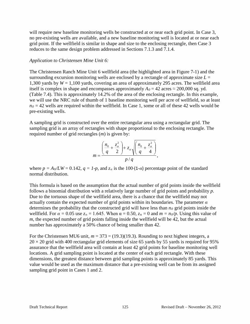
will require new baseline monitoring wells be constructed at or near each grid point. In Case 3, no pre-existing wells are available, and a new baseline monitoring well is located at or near each grid point. If the wellfield is similar in shape and size to the enclosing rectangle, then Case 3 reduces to the same design problem addressed in Sections 7.1.3 and 7.1.4. Application to Christensen Mine Unit 6: The Christensen Ranch Mine Unit 6 wellfield area (the highlighted area in Figure 7-1) and the surrounding excursion monitoring wells are enclosed by a rectangle of approximate size L = 1,300 yards by W = 1,100 yards, covering an area of approximately 295 acres. The wellfield area itself is complex in shape and encompasses approximately A0 = 42 acres ≈ 200,000 sq. yd. (Table 7.4). This is approximately 14.2% of the area of the enclosing rectangle. In this example, we will use the NRC rule of thumb of 1 baseline monitoring well per acre of wellfield, so at least n0 = 42 wells are required within the wellfield. In Case 1, some or all of these 42 wells would be pre-existing wells. A sampling grid is constructed over the entire rectangular area using a rectangular grid. The sampling grid is an array of rectangles with shape proportional to the enclosing rectangle. The required number of grid rectangles (m) is given by:
qp
zqnzz
qn
m/
42
20
20
++
+
=
αα
α
,
where p = A0/LW = 0.142, q = 1-p, and zα is the 100∙(1-α) percentage point of the standard normal distribution. This formula is based on the assumption that the actual number of grid points inside the wellfield follows a binomial distribution with a relatively large number of grid points and probability p. Due to the tortuous shape of the wellfield area, there is a chance that the wellfield may not actually contain the expected number of grid points within its boundaries. The parameter α determines the probability that the constructed grid will have less than n0 grid points inside the wellfield. For α = 0.05 use zα = 1.645. When α = 0.50, zα = 0 and m = n0/p. Using this value of m, the expected number of grid points falling inside the wellfield will be 42, but the actual number has approximately a 50% chance of being smaller than 42. For the Christensen MU6 unit, m = 373 = (19.3)(19.3). Rounding to next highest integers, a 20 × 20 grid with 400 rectangular grid elements of size 65 yards by 55 yards is required for 95% assurance that the wellfield area will contain at least 42 grid points for baseline monitoring well locations. A grid sampling point is located at the center of each grid rectangle. With these dimensions, the greatest distance between grid sampling points is approximately 85 yards. This value would be used as the maximum distance that a pre-existing well can be from its assigned sampling grid point in Cases 1 and 2.
Draft Technical Report 125 Revised Draft – November 26, 2012

7.1.3 Determining the Number of Baseline Samples The selection and location of the baseline sampling wells was discussed in the previous section. This section provides a statistical approach for determining the required number of baseline samples. A sufficient number of wells should be sampled to ensure that the baseline is adequately characterized. In this document, adequacy of the baseline characterization is measured by the precision of the estimates of the baseline parameter values. The goal of the baseline sampling design is to estimate the mean baseline concentrations of all analytes of concern to within a specified level of precision. The required level of precision is obtained by having a sufficient number of samples to reduce the relative standard error of the mean to within acceptable levels. If there is a large degree of heterogeneity in the baseline concentrations in different sections of the production unit, it may not be possible to reduce the relative error of the mean to the specified level. In that case, it may be necessary to divide the unit into several survey units comprised of contiguous areas with similar baseline characteristics for the analytes of greatest concern. In this case, the decisions on compliance with baseline levels would be developed separately for each survey unit. Relative Standard Error of the Mean The population coefficient of variation cv = S/M is useful because the population standard deviation S must always be considered in the context of the population mean M. The value of the coefficient of variation is independent of the dimensions of the measurement and is a dimensionless number. By convention, the coefficient of variation is expressed as a percentage, where cv = 100% is equivalent to cv = 1.0. For comparison between analytes with different units or widely different means, the coefficient of variation provides a standardized measure of variability of the populations. The same advantages apply to the standard error of estimation of the mean SEM, which is equal
to S / N . The coefficient of variation of an estimated mean, denoted here by COVM is the ratio of the standard error of the mean to the mean itself COVM = SEM/M. The coefficient of variation of the mean is often expressed as a percentage. When expressed as a percentage, the term “relative standard error of the mean” will be used, denoted by the symbol RSEM. Thus, RSEM = 100% is equivalent to COVM = 1.0. For comparison between analytes with different units or widely different means, the RSEM provides a standardized, unit-free non-negative numerical value for comparing the precision with which the mean concentrations of multiple analytes have been measured. The value of RSEM depends on both the standard deviation of the population S and the number of samples N. The standard deviation is a measure of variability, and the variability in the samples depends on many factors including temporal and spatial variations in properties of the ore zone environment, well sampling methods, and laboratory measurement error. Many of these sources of variability are beyond the control of the site operator. As variability depends on site-specific characteristics, specific baseline sample sizes for a production unit cannot be determined in advance without sufficient prior data to provide at least a rough estimate of the standard deviation. Some potential constituents, particularly radionuclides and other matrix characteristics
Draft Technical Report 126 Revised Draft – November 26, 2012

that affect the rate of extraction, may already have been measured during site exploration and development and provide a reasonable sample size for estimating the standard deviation. Other constituents may already have been monitored at nearby sites or sites with similar geochemical characteristics. Others may have no historical background databases and require a round of preliminary baseline sampling before the required sample size can be determined.
Table 7-2 contains summary statistics for the population coefficient of variation cv collected at nine sites for 35 analytes.14 The average coefficient of variation ranges from 4% to over 250% in this table. The upper part of this table shows the ranked statistics for analytes other than the trace metals, which are shown in the lower part of the table. Analytes other than trace metals with the highest coefficient of variation include NO2
-, CO3-2, U, NH4
+, and Ra-226. Of this list, only CO3
-2, U, and Ra-226 have a large fraction of measurements above the detection limit. Trace metals with the highest coefficient of variation include aluminum, iron, selenium, and manganese. Among these, only iron has a large fraction of measurements over the detection limit. Although many of the sources of variability are beyond the control of the site operator, increasing the number of baseline samples provides a way to control the RSEM for all analytes of concern to within acceptable levels. Table 7-3 shows an example of the RSEM approach. This table provides the information required to control the degree of precision obtained for mean baseline concentrations of 35 analytes at Christensen Ranch Mine Unit 6 (COGEMA 1996).
Baseline water quality sampling was conducted according to the requirements approved in the Christensen Ranch Amendment Application. The application required four rounds of sampling. The sampling was conducted over a short, 6-week period in the summer of 1996. Sampling events were spaced 2 weeks apart; 2 of the 4 samples from each baseline well were analyzed for a full suite of chemical parameters, while the remaining 2 samples were analyzed for a shorter list of constituents. The 4 rounds of analytical results from the 42 baseline wells were combined to establish baseline water quality. Table 7-2 provides a summary of the combined analytical results from the baseline wells. The list of 35 analytes in Table 7-3 includes the concentrations of major ions, trace metals, and radionuclides and other aquifer properties such as pH, alkalinity, conductivity, and total dissolved solids (TDS).
The table shows the number of samples used to compute the baseline mean and standard deviation, and the standard error and relative standard error of the mean for each analyte. At this site, up to 168 samples were used to characterize the baseline. The RSEM obtained for the analytes ranges from 0.3% to 7%. The radionuclides (U and Ra-226) are among the highest RSEM percentages; 6.8% for U and 6.6% for Ra-226. Several trace metals, including iron and aluminum, are also among the highest percentages. The high RSEM values indicate that these analytes were measured with the least relative precision.
14 Sources: Crow Butte MU1 (Crow Butte 2000, Table 2); Highland A (Kearney 2004, Attachment A, Appendix 3); Highland B (Power Resources 2004, Table 1); Irigaray MU1 to MU9 (Wichers 2006, Table 1); Christensen MU2 North (Total Resources 1993, Table 2); Christensen MU3 (Malapai 1988, Table 2); Christensen MU4 (COGEMA 1994, Table 6); Christensen MU5 (COGEMA 1995, Table 7); and Christensen MU6 (COGEMA 1996, Table 6).
Draft Technical Report 127 Revised Draft – November 26, 2012

Figure 7-1. Ore Zone Outline and Well Locations at Christensen Ranch Mine Unit 6 The required number of baseline samples to achieve a precision of P% is calculated using:
( ) ( )22 // PcMPSN v== where cv and P are expressed in percentage terms. For example, in Table 7-2, uranium has an average coefficient of variation of 105%. The required number of samples to estimate the mean uranium concentration with a precision of P = ±10% is:
( ) ( ) 11010/105/ 22 === PcN v
Draft Technical Report 128 Revised Draft – November 26, 2012

The right side of Table 7-3 shows the number of samples required for each analyte to achieve a targeted RSEm of P%, for values of P ranging from 1% up to 100%. At Mine Unit 6, uranium and Ra-226 require the largest number of samples to achieve the targeted level of precision. For example, 75 samples are required to achieve a hypothetical target precision of P = 10% for uranium, and 74 samples are required for Ra-226. These sample sizes are the highest required to achieve a target precision of P = 10% for all listed analytes. If 75 or more baseline samples are collected at the mine unit, then the RSEM for all analytes is expected to be less than the target value of P = 10%. With at least 167 baseline samples for uranium and Ra-226 at Mine Unit 6, the achieved RSEM for U and Ra-226 is considerably less than 10% for both radionuclides. Table 7-4 shows the results of similar analyses conducted for nine ISR sites.15 This table summarizes results of the analyses, with emphasis on the RSEM achieved for the mean baseline uranium and Ra-226 concentrations at each site. The table also shows the size, number of baseline wells, number of wells per acre, and the average number of baseline samples per well. The right side of this table contains the actual sample size and achieved precision for uranium and Ra-226. This table also shows the sample sizes that would be required for a hypothetical targeted precision of ±10%. The highlighting in this table indicates sites meeting a hypothetical targeted precision goal of ±10%. Table 7-5 contains the summary information for uranium and Ra-226 found in the bottom two rows of Table 7-3 for nine ISR sites. The table shows the number of samples required for the RSEM for uranium and Ra-226 to be less than ±P%. The table also shows the actual number of baseline samples and the achieved precision for uranium and Ra-226 at each site. Figure 7-2 contains a scatter plot of the maximum RSEM for uranium and Ra-226 mean concentrations versus the baseline sample size at the nine production units listed in Table 7-5. A baseline sample size of approximately 80 to 100 samples is sufficient to achieve a precision of ±10% at the sites examined. NRC’s current expectations regarding baseline sampling in the ore zone are set out in their Standard Review Plan for ISR license applications (NRC 2003, p. 5-39), which specifies that one well per acre should be sampled with four independent samples taken from each well. If a typical wellfield is 25 acres, then 100 baseline samples would be required. Using the RSEM approach presented here and assuming that a DQO for the RSEM is fixed at ±10% and the ratio of the sample mean to the sample standard deviation is 1.0, then the required number of samples would be 100 or the same as current practice for a typical wellfield. This hypothetical example is supported by Figure 7-2, which shows, using actual sites, that a baseline sample size of approximately 80 to 100 samples is sufficient to achieve a precision of ±10% at the sites examined. If the DQO is reduced to ±5%, the theoretical sample size would be increased to 400. Any additional sampling could be accommodated by various combinations of additional wells, extending the sampling period, RSEM or increasing the sampling frequency. However, the operator must insure that the additional samples are independent in space and time. For example, if additional baseline sampling wells are required, they should be located in the ore zone as far as possible from other baseline sampling wells. If more samples are required from each baseline well, the additional sampling times should be roughly mid-way between current sampling times. Frequency of sampling should not exceed eight samples per year per well.
15 See Footnote 9 for sources of data.
Draft Technical Report 129 Revised Draft – November 26, 2012

7.1.4 Summary In practice, the following approach might be taken to determine the number of baseline samples:
• The regulator establishes the DQO for the RSEM (e.g., ±10%).
• The operator collects periodic samples for 1 year based on a sample density of one per acre per sampling. (From Table 7-4, it is likely that larger wellfields may require quarterly sampling, while smaller wellfields (e.g., less than 20 acres) may require monthly sampling.)
• The operator calculates the RSEM for each analyte by pooling sampling results.
• Unless the sampling results suggest otherwise, the operator determines whether either uranium or Ra-226 has an RSEM exceeding the DQO.
• If either uranium or Ra-226 exceeds the DQO, the operator continues sampling until the DQO is achieved.
This approach is based on the assumptions that uranium and Ra-226 are key analytes in understanding the ground water chemistry, that they will have few nondetects in the baseline sampling program, and that, based on the data reported here, they typically have high variability.
Table 7-2. Summary Statistics for Population Coefficient of (cv) of Baseline Parameters at Nine ISR Sites
Variation
Rank Analyte Number of Sites Minimum cv Average cv Maximum cv
1 NO2 Major Ions (mg/
2 L) and Radiometrics
97% 121% 145% 2 CO3 8 43% 110% 327% 3 U mg/L 9 42% 105% 213% 4 NH4 7 11% 105% 433% 5 Ra-226 pCi/L 9 61% 75% 87% 6 NO3 7 6% 56% 222% 7 K 9 12% 47% 93% 8 Mg 9 7% 38% 129% 9 Ca 9 1% 21% 52%
10 F 9 6% 18% 35% 11 Cl 9 7% 15% 36% 12 HCO3 9 3% 12% 25% 13 SiO2 9 3% 12% 23% 14 Alk 9 3% 9% 27% 15 SO4 9 3% 8% 16% 16 Cond 9 3% 7% 14% 17 TDS 9 2% 6% 12% 18 Na 9 3% 5% 9% 19 pH 9 2% 4% 7%
Draft Technical Report 130 Revised Draft – November 26, 2012

Table 7-2. Summary Statistics for Population Coefficient of Variation (cv) of Baseline Parameters at Nine ISR Sites
Rank Analyte Number of Sites Minimum cv Average cv Maximum cv Trace Metals (mg/L)
1 Al 2 65% 262% 459% 2 Fe 3 62% 253% 406% 3 Se 7 50% 208% 581% 4 Mn 4 38% 127% 206% 5 V 3 55% 103% 155% 6 Cr 1 95% 95% 95% 7 As 6 33% 93% 285% 8 Cd 2 70% 85% 100% 9 Hg 1 83% 83% 83%
10 Pb 1 83% 83% 83% 11 Cu 3 37% 82% 110% 12 Ni 2 28% 65% 102% 13 Zn 5 33% 50% 91% 14 Ba 1 39% 39% 39% 15 B 2 4% 25% 46% 16 Mo 2 9% 24% 40%
Draft Technical Report 131 Revised Draft – November 26, 2012
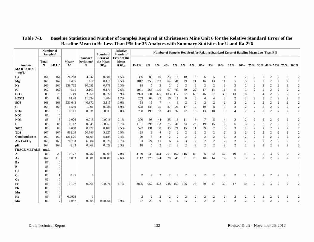
Table 7-3. Baseline Statistics and Number of Samples Required at Christensen Mine Unit 6 for the Relative Standard Error of the Baseline Mean to Be Less Than P% for 35 Analytes with Summary Statistics for U and Ra-226
Analyte
Number of Samples*
Mean* M
Standard Deviation*
S
Standard Error of the Mean
SEM
Relative Standard
Error of the Mean RSEM
Number of Samples Required for Relative Standard Error of Baseline Mean Less Than P%
Total N a>D.L. P=1% 2% 3% 4% 5% 6% 7% 8% 9% 10% 15% 20% 25% 30% 40% 50% 75% 100%
MAJOR IONS – mg/L Ca 164 164 26.238 4.947 0.386 1.5% 356 89 40 23 15 10 8 6 5 4 2 2 2 2 2 2 2 2 Mg 166 162 4.455 1.417 0.110 2.5% 1012 253 113 64 41 29 21 16 13 11 5 3 2 2 2 2 2 2 Na 168 168 239.762 10.091 0.779 0.3% 18 5 2 2 2 2 2 2 2 2 2 2 2 2 2 2 2 2 K 162 162 6.61 2.163 0.170 2.6% 1071 268 119 67 43 30 22 17 14 11 5 3 2 2 2 2 2 2 CO3 85 78 5.49 2.968 0.322 5.9% 2923 731 325 183 117 82 60 46 37 30 13 8 5 4 2 2 2 2 HCO3 85 83 74.48 11.834 1.284 1.7% 253 64 29 16 11 8 6 4 4 3 2 2 2 2 2 2 2 2 SO4 168 168 530.643 40.372 3.115 0.6% 58 15 7 4 3 2 2 2 2 2 2 2 2 2 2 2 2 2 Cl 168 168 4.539 1.091 0.084 1.9% 578 145 65 37 24 17 12 10 8 6 3 2 2 2 2 2 2 2 NH4 86 19 0.111 0.031 0.0033 3.0% 780 195 87 49 32 22 16 13 10 8 4 2 2 2 2 2 2 2 NO2 86 0 NO3 86 5 0.076 0.015 0.0016 2.1% 390 98 44 25 16 11 8 7 5 4 2 2 2 2 2 2 2 2 F 85 85 0.142 0.049 0.0053 3.7% 1191 298 133 75 48 34 25 19 15 12 6 3 2 2 2 2 2 2 SiO2 86 86 4.058 0.927 0.100 2.5% 522 131 58 33 21 15 11 9 7 6 3 2 2 2 2 2 2 2 TDS 167 167 861.09 50.746 3.927 0.5% 35 9 4 3 2 2 2 2 2 2 2 2 2 2 2 2 2 2 Cond μmho/cm 167 167 1261.26 66.99 5.184 0.4% 29 8 4 2 2 2 2 2 2 2 2 2 2 2 2 2 2 2 Alk CaCO3 166 166 70.753 6.804 0.528 0.7% 93 24 11 6 4 3 2 2 2 2 2 2 2 2 2 2 2 2 pH 164 164 8.83 0.369 0.029 0.3% 18 5 2 2 2 2 2 2 2 2 2 2 2 2 2 2 2 2 TRACE METALS – mg/L Al 86 20 0.127 0.082 0.009 7.0% 4169 1043 464 261 167 116 86 66 52 42 19 11 7 5 3 2 2 2 As 167 118 0.003 0.001 0.00008 2.6% 1112 278 124 70 45 31 23 18 14 12 5 3 2 2 2 2 2 2 Ba 86 0 B 86 0 Cd 86 0 Cr 86 1 0.05 0 2 2 2 2 2 2 2 2 2 2 2 2 2 2 2 2 2 2 Cu 86 0 Fe 86 3 0.107 0.066 0.0071 6.7% 3805 952 423 238 153 106 78 60 47 39 17 10 7 5 3 2 2 2 Pb 86 0 Mn 86 0 Hg 86 3 0.0003 0 2 2 2 2 2 2 2 2 2 2 2 2 2 2 2 2 2 2 Mo 86 7 0.057 0.005 0.00054 0.9% 77 20 9 5 4 3 2 2 2 2 2 2 2 2 2 2 2 2
Draft Technical Report 132 Revised Draft – November 26, 2012

Table 7-3. Baseline Statistics and Number of Samples Required at Christensen Mine Unit 6 for the Relative Standard Error of the Baseline Mean to Be Less Than P% for 35 Analytes with Summary Statistics for U and Ra-226
Analyte
Number of Samples*
Mean* M
Standard Deviation*
S
Standard Error of the Mean
SEM
Relative Standard
Error of the Mean RSEM
Number of Samples Required for Relative Standard Error of Baseline Mean Less Than P%
Total N a>D.L. P=1% 2% 3% 4% 5% 6% 7% 8% 9% 10% 15% 20% 25% 30% 40% 50% 75% 100%
Ni 86 4 0.068 0.019 0.0020 3.0% 781 196 87 49 32 22 16 13 10 8 4 2 2 2 2 2 2 2 Se 168 13 0.0020 0.001 0.00008 3.9% 2500 625 278 157 100 70 52 40 31 25 12 7 4 3 2 2 2 2 V 86 3 0.107 0.059 0.0064 5.9% 3041 761 338 191 122 85 63 48 38 31 14 8 5 4 2 2 2 2 Zn 86 21 0.015 0.008 0.00086 5.8% 2845 712 317 178 114 80 59 45 36 29 13 8 5 4 2 2 2 2 RADIOMETRICS U mg/L 164 148 0.0126 0.0109 0.00085 6.8% 7484 1871 832 468 300 208 153 117 93 75 34 19 12 9 5 3 2 2 Ra-226 pCi/L 168 167 105.858 90.928 7.015 6.6% 7379 1845 820 462 296 205 151 116 92 74 33 19 12 9 5 3 2 2 Maximum for
U, Ra-226 P
168
167 -
- - 6.8%
7484 P=1%
1871 2%
832 3%
468 4%
300 5%
208 6%
153 7%
117 8%
93 9%
75 10%
34 15%
19 20%
12 25%
9 30%
5 40%
3 50%
2 75%
2 100%
a - >D.L. is greater than detection limit * Source: COGEMA 1996, Table 6, mean is arithmetic mean for all detectable samples
Draft Technical Report 133 Revised Draft – November 26, 2012

Table 7-4. Wellfield Characteristics and Comparison of Actual and Target Baseline Sample Size at Nine ISR Production Units
Site
Acres
Number
of Baseline
Wells
Number
of Baseline
Wells per Acre
Average Number
of Samples per Well
Target
Number of
Samples per Well*
Maximum
Target Number of Samples for RSEM=10%
U Ra-226
Actual N
Achieved RSEM
Target N
Target RSEM
Actual N
Achieved RSEM
Target N
Target RSEM
Crow Butte MU1 9.3 12 1.3 8.4 8 94 101 9.6% 94 10% 101 7.7% 60 10% Highland A 3.0 5 1.7 1.0 8 38 5 18.6% 18 10% 5 27.4% 38 10% Highland B 13.8 20 1.4 - 24 445 - - 445 10% - - 47 10% Irigaray MU1 to MU9 30 46 1.5 4.3 4 162 200 9.0% 162 10% 200 7.0% 76 10% Christensen MU2 North 5.7 8 1.4 4.0 9 69 32 14.7% 69 10% 32 10.8% 37 10% Christensen MU3 20.4 22 1.1 4.0 6 132 64 14.3% 132 10% 64 8.3% 44 10% Christensen MU4 12 12 1 4.0 14 164 48 18.5% 164 10% 49 11.9% 70 10% Christensen MU5 25 25 1 4.0 3 69 99 5.8% 34 10% 99 8.3% 69 10% Christensen MU6 42 42 1 3.9 2 75 164 6.8% 75 10% 168 6.6% 74 10%
Key Sites meeting hypothetical targeted precision goal of 10%. * An alternative is to increase the number of wells.
Draft Technical Report 134 Revised Draft – November 26, 2012

Table 7-5. Number of Samples Required at Nine Production Units for Relative Standard Error of U and Ra-226 Mean Baseline Concentrations to Be Less Than ±P%
Wells Samples Number of Samples (N) Required for RSEM of U and Ra-226 Baseline Means to Be Less Than ±P% Site per per Acre Well P=1% 2% 3% 4% 5% 6% 7% 8% 9% 10% 15% 20% 25% 30% 40% 50% 75% 100%
Crow Butte MU1 1.29 8.40 9,359 2,340 1,040 585 375 260 191 147 116 94 42 24 15 11 6 4 2 2 Actual P and N for (U, Ra) 9.6% (101,101)
Highland A 1.67 1.00 3,741 936 416 234 150 104 77 59 47 38 17 10 6 5 3 2 2 2 Actual P and N for (U, Ra) 27.4% (5,5)
Highland B 1.38 - 45,374 11,344 5,042 2,836 1,815 1,261 926 709 561 454 202 114 73 51 29 19 9 5 Actual P and N for (U, Ra)
Irigaray MU1-9 1.53 4.35 16,127 4,032 1,792 1,008 646 448 330 252 200 162 72 41 26 18 11 7 3 2 Actual P and N for (U, Ra) 9% (200,200)
Christensen MU2 North 1.40 4.00 6,877 1,720 765 430 276 192 141 108 85 69 31 18 12 8 5 3 2 2 Actual P and N for (U, Ra) 14.7% (32,32)
Christensen MU3 1.08 4.00 13,142 3,286 1,461 822 526 366 269 206 163 132 59 33 22 15 9 6 3 2 Actual P and N for (U, Ra) 14.3% (64,64)
Christensen MU4 1.00 4.00 16,352 4,088 1,817 1,022 655 455 334 256 202 164 73 41 27 19 11 7 3 2 Actual P and N for (U, Ra) 18.5% (48,49)
Christensen MU5 1.00 3.96 6,838 1,710 760 428 274 190 140 107 85 69 31 18 11 8 5 3 2 2 Actual P and N for (U, Ra) 8.3% (99,99)
Christensen MU6 1.00 3.90 7,484 1,871 832 468 300 208 153 117 93 75 34 19 12 9 5 3 2 2 Actual P and N for (U, Ra) 6.8% (164,168)
Summary Statistics Across All Sites
Wells per
Acre
Samples per
Well
Number of Samples (N) Required for Coefficients of Variation of U and Ra-226 Baseline Means to Be Less Than ±P%
P=1% 2% 3% 4% 5% 6% 7% 8% 9% 10% 15% 20% 25% 30% 40% 50% 75% 100%
Average 1.24 4.18 13,922 3,481 1,547 870 557 387 285 218 172 140 62 35 23 16 9 6 3 2
Minimum 1.00 1.00 3,741 936 416 234 150 104 77 59 47 38 17 10 6 5 3 2 2 2
Maximum 1.67 8.40 45,374 11,344 5,042 2,836 1,815 1,261 926 709 561 454 202 114 73 51 29 19 9 5
Draft Technical Report 135 Revised Draft – November 26, 2012
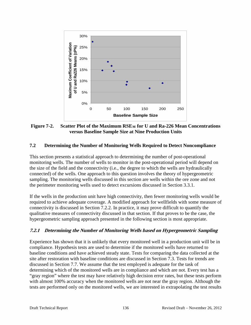
30%
25%tion
rians
(±P%
)
20%
ea15%
nt o
f Va
a M
Max
imum
Coe
ffici
e o
f U22
6 a
nd R
10%
5%
0%0 50 100 150 200 250
Baseline Sample Size
Figure 7-2. Scatter Plot of the Maximum RSEM for U and Ra-226 Mean Concentrations versus Baseline Sample Size at Nine Production Units
7.2 Determining the Number of Monitoring Wells Required to Detect Noncompliance This section presents a statistical approach to determining the number of post-operational monitoring wells. The number of wells to monitor in the post-operational period will depend on the size of the field and the connectivity (i.e., the degree to which the wells are hydraulically connected) of the wells. One approach to this question involves the theory of hypergeometric sampling. The monitoring wells discussed in this section are wells within the ore zone and not the perimeter monitoring wells used to detect excursions discussed in Section 3.3.1. If the wells in the production unit have high connectivity, then fewer monitoring wells would be required to achieve adequate coverage. A modified approach for wellfields with some measure of connectivity is discussed in Section 7.2.2. In practice, it may prove difficult to quantify the qualitative measures of connectivity discussed in that section. If that proves to be the case, the hypergeometric sampling approach presented in the following section is most appropriate. 7.2.1 Determining the Number of Monitoring Wells based on Hypergeometric Sampling Experience has shown that it is unlikely that every monitored well in a production unit will be in compliance. Hypothesis tests are used to determine if the monitored wells have returned to baseline conditions and have achieved steady state. Tests for comparing the data collected at the site after restoration with baseline conditions are discussed in Section 7.3. Tests for trends are discussed in Section 7.7. We assume that the test employed is adequate for the task of determining which of the monitored wells are in compliance and which are not. Every test has a “gray region” where the test may have relatively high decision error rates, but these tests perform with almost 100% accuracy when the monitored wells are not near the gray region. Although the tests are performed only on the monitored wells, we are interested in extrapolating the test results
Draft Technical Report 136 Revised Draft – November 26, 2012
obtained for the monitored wells to other wells in the production unit, assuming they would have a similar pattern of test outcomes if all wells were monitored.
If the test outcomes indicate that all monitored wells demonstrate compliance, or if only a few do not, then these results also provide information about the wells which were not monitored. Suppose the question is phrased in this manner:
If all wells were monitored, what percentage of the wells would be expected to not demonstrate compliance?
If all wells were monitored, this percentage would be known. When fewer than all wells are monitored, the percentage can be known only with uncertainty. The statistical approach involves confidence levels for the unknown parameter Q defined as the percentage of wells that would not demonstrate compliance if all wells were monitored.16 The compliance determinations for the monitored wells are based on statistical tests that will have Type 1 and Type 2 errors. Hence, a test indicating that a monitored well is in compliance does not mean that the well truly is in compliance, and a test indicating that a monitored well is not in compliance does not mean that the well truly is not in compliance. This limitation also is applicable for Q, which is a measure of the proportion of wells with test results that are not in compliance.
In the following discussion, the set of all wells in the production unit form the “population” from which a “sample” of monitored wells is selected. In many sampling problems, it is assumed that the population to be sampled is much larger than the intended size of the sample. Essentially, the population size is assumed to be of infinite size. When a population of finite size is sampled, the required size of the sample is less than the corresponding sample size for an infinite population. In a population with a relatively small size (in the hundreds), the savings can be significant. With a population of finite size, it is theoretically possible to determine exactly any population parameter of interest by monitoring all of the wells. When only a sample of wells is monitored, then population parameter estimates will have uncertainty and a statistical approach is used for estimating these parameters.
There are several statistical approaches for estimating the population parameter Q. Two parametric statistical approaches are the traditional frequentist statistical approach, such as maximum likelihood estimation and the Bayesian approach.
In maximum likelihood estimation, the goal is to find the “best” point estimate for Q, defined as the value of Q which maximizes the likelihood function l(Q, X) for the observed set of sample values X=(x1, …, xn). This estimate is a “statistic,” meaning that it depends on the sample values X. The most commonly used maximum likelihood estimate is the sample mean. Since this estimate is a function of the sample values, the estimate would vary if the sampling process was
16 The percentage of wells that are not in compliance is an observable parameter that serves as a surrogate for the question of greater interest: What percentage of the underlying aquifer is not in compliance? The interlaced, 5-spot and 7-spot patterns of injection/extraction wells serve as an efficient sampling grid for monitoring the underlying aquifer(s). If geostatistical software is available, indicator kriging may be used to estimate the percent of compliance throughout the unit.
Draft Technical Report 137 Revised Draft – November 26, 2012
repeated. Confidence intervals for the “true” value of Q are formed by calculating the frequency of values of Q that would occur when the sampling process is repeated. In the Bayesian approach, it is assumed that the value of the population parameter Q is always uncertain, both before and after the sampling process. It is also assumed that this uncertainty can be expressed in the form of a probability distribution for the unknown parameter Q. This probability distribution expresses the uncertainty in the estimate of Q. If Q is relatively well known, then the probability distribution is a narrow distribution, but if the value of Q is very uncertain, then the probability distribution is wide. Before the sampling is done, the prior state of knowledge about the parameter Q is expressed in a prior distribution written as p(Q). After the sampling is completed, the data are used to update the prior state of knowledge about the parameter Q (using Bayes’ theorem) to a new, narrower distribution called the posterior distribution p(Q|X). The posterior distribution is proportional to the product of the prior distribution times the likelihood function: p(Q|X) ≈ p(Q) l(Q, X) In this application, a non-informative prior distribution is used for Q. The only prior knowledge assumed is that Q must be between 0 and 1, and no value of Q in between these limits is more likely that any other value. These assumptions imply that the prior distribution for Q is a uniform distribution between 0 and 1, i.e., p(Q)=1 for all Q. Note that p(Q|X) ≈ l(Q, X) with this choice of a prior distribution. The value of Q, which maximizes the likelihood function, is the same value that maximizes the Bayesian posterior distribution for Q. Hence, the maximum likelihood estimate is equal to the Bayesian highest posterior density estimate using a non-informative prior distribution. In addition to the point estimate generated using the Bayesian approach, both 1-sided and 2-sided intervals of highest posterior density (HPD) may be constructed containing 90%, 95% or any desired level of posterior probability. The shape of the posterior distribution is, in general, not symmetric around the highest posterior density point estimate. This means that the HPD intervals for Q constructed using the Bayesian approach are in general asymmetric. The degree of asymmetry increases at values of Q near 0 or 1. The HPD intervals are approximately symmetric when Q is near ½. In this section, it is assumed that a sufficient number of samples have been collected from each monitored well to determine if the well demonstrates compliance. (Sections 7.6 and 7.8 discuss the procedures for determining compliance of an individual well.) After the sampling is completed, some of the monitored wells will have demonstrated compliance and others will not. These results are used to determine the maximum likelihood (and Bayesian) point estimate of Q equal to the percentage of monitored wells not demonstrating compliance:
( )( ) ( )Ncompliance showingnot wellsmonitored of #100Q̂ = This point estimate of Q will have statistical uncertainty. The required number of monitoring
ells is determined by placing an upper bound on the posterior distribution for Q. If there are M ells in a production unit, then a sufficient number N are designated as monitoring wells, such
hat the Bayesian 1-sided highest posterior density interval for Q is within the specified bounds.
wwt
Draft Technical Report 138 Revised Draft – November 26, 2012

If all monitored wells are found to demonstrate compliance, then the point estimate for Q is 0%. However, this estimate also has uncertainty, as there still may be unmonitored wells that would be expected not to demonstrate compliance. If a well production unit has only 5 wells, then monitoring of all wells may be required to achieve the desired level of confidence in the estimate of Q. If there are 200 wells in a production unit, it will be necessary to monitor more than 5 wells, but not to monitor all the wells. However, if the number of noncomplying wells in the unit is small relative to M, it is very difficult to detect that there are wells out of compliance without very extensive monitoring. A Bayesian analysis of the hypergeometric distribution is used to determine the number of monitoring wells required to demonstrate, with a relatively high degree of assurance, that no more than q percent of the wells in the field would not demonstrate compliance if all wells were monitored. Let X denote the number of monitored wells that do not demonstrate compliance in the set of N monitoring wells. Let Y denote the unknown number of wells in the field that would not show compliance if all wells were tested. Then the random variable X has a hypergeometric distribution with parameters N, M and Y. A realization of the random variable X is a nonnegative integer denoted by the lower case symbol x. Table 7-6 shows the parameters of the hypergeometric distribution and the range of values for each parameter.
Table 7-6. Parameter Definitions for the Hypergeometric Distribution All Wells in Production Unit Monitored Wells in Production Unit Parameter (Population) (Sample)
M N Number of Wells M>0 1≤N≤M Number of Wells not Y X Showing Compliance x ≤y≤
M max(0,N-M+y) ≤ x ≤ min(N, y)
A “sample” of N monitoring wells should be selected from the total number of wells. The monitoring wells should be representative of the “population” of all M wells in the production unit. Using the hypergeometric distribution, the probability that x of the N monitored wells do not show compliance, given that Y=y of all M wells in the production unit do not show compliance, is:
−−
===
NM
xNyM
xy
NMyYxXP ],,|[ .
Here the combinatorial coefficient = a! b!(a − b)! for a ≥ b, and the symbol a! denotes the b
factorial of the integer a = (1)(2)(3)…(a). By convention, 0! = 1. Note that the term (M-y) is the number of wells in the production unit that would demonstrate compliance if all wells were tested, and (N-x) is the number of monitored wells that demonstrate compliance. For ease of discussion, we denote a test outcome that demonstrates compliance as a ”Pass;” otherwise, the test outcome is a “Fail.” The posterior distribution for the (unknown) number of
a
Draft Technical Report 139 Revised Draft – November 26, 2012
wells Y in the population with outcome “Fail,” given that x wells had the outcome “Fail” in the sample of N wells, is:
)]!()[()!(
)!(!],,|[
xNyMyM
xyykNMxyYP
−−−−
−==
with ∑ ==y
NMxyYPk ],,|[1 .
Here Y is a random variable with integer values y = x, … , M - (N - x), the posterior distributionP[Y = y | x, M , N ] gives the probability of each possible value of Y, and k is a normalizing constant such that these probabilities add to one. The parameter Q is the unknown percentage of wells in the population that would have an outcome of “Fail” if all wells had been monitored. For each field size M there are M+1 discrete values possible for Q, one for each possible value of Y: Q = 100 j / M , j = 0,, M . The posterior distribution for Q is derived from the posterior distribution for Y by linear transformation. The posterior distribution for Q also depends on x, the number of Fails observed in the monitored wells. It is possible to achieve the desired upper bound on Q using several different monitoring strategies. The strategies are characterized by the upper bound on the number of monitored wells permitted to Fail while still meeting the desired bound on Q. The bound can be achieved by monitoring a smaller number of wells with the requirement that all monitored wells must pass (x=0) to achieve the desired bound on Q. Alternatively, by monitoring a larger number of wells, the same bound on Q can be achieved while allowing for one of the monitored wells to Fail (x=1). The posterior distribution for Q was used to calculate one-sided highest posterior density intervals for Q of the form 0 ≤ Q ≤ q. Table 7-7 and Table 7-8 are derived from the posterior distribution for Q. Table 7-7 is used when all of the monitored wells must Pass, and Table 7-8 is used when one monitored well is permitted to Fail. The number of monitoring wells shown in Table 7-8 is higher than in Table 7-7. Additional tables for obtaining posterior probabilities of 90% and 99% with x=0 or x=1, and tables for achieving posterior probabilities of 90%, 95% and 99% in the case x=2, are found in Tables E-15 through E-21 of Attachment E, respectively. When all monitored wells must “Pass” (x=0), Table 7-7 shows the minimum number of monitoring wells N, such that the probability that Q is less than q is at least 95%, i.e.,
0.95 N} M,0,x | q Q Prob{0 ≥=≤≤ .
If it is determined that all of the N monitored wells “Pass” (i.e., x=0), then there is less than a 5% chance that more than q percent of the wells in the production unit would “Fail” if all M wells were monitored. For example, consider a 5-spot wellfield with approximately 200 wells. With M=200 wells, Table 7-7 indicates that 25 monitoring wells are required for 95% posterior probability that Q is less than 10% if all monitored wells Pass. If 46 wells are monitored and all Pass, there is a 95% probability that Q is less than 5%. If only 17 wells are monitored and all Pass, there is a 95% probability that Q is less than 15%.
Draft Technical Report 140 Revised Draft – November 26, 2012
Table 7-8 shows similar results for the case when one of the monitored wells is permitted to Fail (x=1):
0.95 N} M,,1x | q Q Prob{0 ≥=≤≤ .
If one of the monitored wells is permitted to Fail in the example with M=200 wells, the N=39 monitoring wells would be required to have 95% probability that Q is less than 10%.
As noted above, Q is an unknown parameter defined as the percentage of wells that would not demonstrate compliance if all wells were tested. In order to choose between Table 7-7 and Table 7-8, an estimate of x, the number of monitored wells expected to Fail, is needed. This estimate can be obtained from results of post-restoration sampling, which will likely be done on the baseline wells. The number of baseline wells is currently specified as one well per acre (NRC 2003). If the wellfield has an average area of 25 acres,17 baseline samples and the first round of post-remediation samples would be obtained from 25 wells. Post-restoration sampling of these wells could then be used to estimate x. If all wells demonstrate compliance, then Table 7-7 can be used to determine the number of monitoring wells required to demonstrate that the restored wellfield is in compliance. If x=1, then Table 7-8 should be used. Additional tables for x=2 are included in Attachment E. If x>2, additional restoration would likely be required before proceeding to demonstrate compliance. To determine the number of wells that must be sampled to establish wellfield compliance, DQOs must be set for q, which is the upper bound for Q, and for the probability that Q will not exceed q. If the DQOs are q=5% and Prob{Q ≤ 5%} ≥ 0.95, then using Table 7-7 one can estimate that 52 wells must be monitored in a 25-acre wellfield, with 375 production plus injection wells to satisfy the DQOs. This number is approximately twice the number of baseline wells, so an expanded number of monitoring wells would be required in the post-restoration period. However, if the DQOs are q=10% and Prob{Q ≤ 10%} ≥ 0.95, then 26 wells would require monitoring. This number is approximately equal to the number of baseline wells. Each of the 26 wells in this example would be tested for compliance. If the compliance testing results indicated all of the 26 monitoring wells demonstrate compliance, then there is a 95% probability that no more than 10% of the wells (or, by extension, roughly 10% of the wellfield ground water) would not demonstrate compliance if all wells were tested. If one of the monitored wells is permitted to not demonstrate compliance, then using the Table 7-8 DQOs of q=10% and Prob{Q ≤ 10%} ≥ 0.95 can be achieved by monitoring 42 wells. The number of samples required per well during the post-restoration sampling period is discussed in Section 7.6.
Draft Technical Report 141 Revised Draft – November 26, 2012
17 Based on a survey of a number of ISL sites, an average wellfield was 25 acres and contained about 15
wells per acre, for a total of 375 wells.
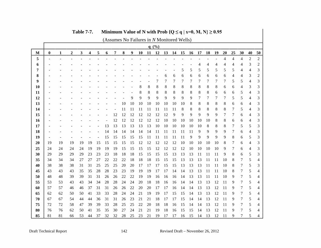
Table 7-7.
M 0 1 2 3 4 5 - - - - -
Minimum Value of N with Prob {Q ≤ q | x=0, M, N} ≥ 0.95 (Assumes No Failures in N Monitored Wells)
q (%) 5 6 7 8 9 10 11 12 13 14 15 16 17 18 19 20 25 30 40 50 - - - - - - - - - - - - - - - 4 4 4 2 2
6 - - - - - - - - - - - - - - - - - 4 4 4 4 4 4 3 2 7 - - - - - - - - - - - - - - - 5 5 5 5 5 5 5 4 4 3 8 - - - - - - - - - - - - - 6 6 6 6 6 6 6 6 4 4 3 2 9 - - - - - - - - - - - - 7 7 7 7 7 7 7 7 7 5 5 4 3
10 - - - - - - - - - - 8 8 8 8 8 8 8 8 8 8 6 6 4 3 3 11 - - - - - - - - - - 8 8 8 8 8 8 8 8 8 6 6 6 5 4 3 12 - - - - - - - - - 9 9 9 9 9 9 9 9 7 7 7 7 5 5 4 3 13 - - - - - - - - 10 10 10 10 10 10 10 10 8 8 8 8 8 6 6 4 3 14 - - - - - - - - 11 11 11 11 11 11 11 8 8 8 8 8 8 7 5 4 3 15 - - - - - - - 12 12 12 12 12 12 12 9 9 9 9 9 9 7 7 6 4 3 16 - - - - - - - 12 12 12 12 12 12 10 10 10 10 10 10 8 8 6 6 4 3 17 - - - - - - 13 13 13 13 13 13 10 10 10 10 10 10 8 8 8 7 5 5 3 18 - - - - - - 14 14 14 14 14 14 11 11 11 11 11 9 9 9 9 7 6 4 3 19 - - - - - - 15 15 15 15 15 11 11 11 11 11 9 9 9 9 9 8 6 5 3 20 19 19 19 19 19 15 15 15 15 15 12 12 12 12 12 10 10 10 10 10 8 7 6 4 3 25 24 24 24 24 19 19 19 19 15 15 15 15 12 12 12 12 10 10 10 10 9 7 6 4 3 30 29 29 29 29 23 23 23 18 18 18 15 15 15 15 13 13 13 11 11 11 9 8 6 5 3 35 34 34 34 27 27 27 22 22 22 18 18 18 15 15 15 13 13 13 11 11 10 8 7 5 4 40 38 38 38 31 31 25 25 25 20 20 17 17 17 15 15 13 13 13 11 11 10 8 7 5 3 45 43 43 43 35 35 28 28 23 23 19 19 19 17 17 14 14 13 13 11 11 10 8 7 5 4 50 48 48 39 39 31 31 26 26 22 22 19 19 16 16 16 14 13 13 11 11 10 9 7 5 4 55 53 53 43 43 34 34 28 28 24 24 20 18 18 16 16 14 14 13 13 12 11 9 7 5 4 60 57 57 46 46 37 31 31 26 26 22 20 20 17 17 16 14 14 13 13 12 11 9 7 5 4 65 62 62 50 50 41 33 33 28 24 24 21 19 19 17 15 15 14 13 13 12 11 9 7 5 4 70 67 67 54 44 44 36 31 31 26 23 21 21 18 17 17 15 14 14 13 12 11 9 7 5 4 75 72 72 58 47 39 39 33 28 25 25 22 20 18 18 16 15 14 14 13 12 11 9 7 5 4 80 76 76 62 50 41 35 35 30 27 24 21 21 19 18 16 15 15 14 13 12 11 9 7 5 4 85 81 81 66 53 44 37 32 32 28 25 23 21 19 17 17 16 15 14 13 12 11 9 7 5 4
Draft Technical Report 142 Revised Draft – November 26, 2012
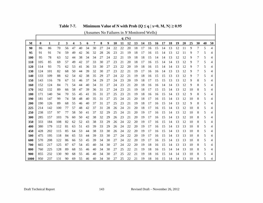
Table 7-7. Minimum Value of N with Prob {Q ≤ q | x=0, M, N} ≥ 0.95 (Assumes No Failures in N Monitored Wells)
q (%) M 0 1 2 3 4 5 6 7 8 9 10 11 12 13 14 15 16 17 18 19 20 25 30 40 50 90 86 86 70 56 47 40 34 30 27 24 22 22 20 18 17 16 15 14 13 12 11 9 7 5 4 95 91 91 74 59 49 42 36 32 28 26 23 21 19 18 17 16 15 14 13 12 11 9 7 5 4
100 95 78 63 52 44 38 34 34 27 24 22 21 19 18 18 15 14 14 13 12 12 9 7 5 4 110 105 85 69 57 49 42 37 33 30 27 23 21 20 18 17 16 15 14 14 13 12 9 7 5 4 120 114 93 75 62 53 41 36 33 30 27 23 22 20 19 18 16 15 14 14 13 12 9 7 5 4 130 124 101 82 68 50 44 39 32 30 27 23 22 21 19 17 16 16 14 13 13 12 9 7 5 4 140 133 109 88 62 54 42 38 35 29 27 24 22 21 19 18 16 15 15 13 13 12 9 7 5 4 150 143 116 78 67 51 46 37 34 29 27 24 23 20 19 18 17 15 15 13 13 12 9 8 5 4 160 152 124 84 71 54 44 40 34 31 27 24 23 21 20 18 16 16 14 14 13 12 9 8 5 4 170 162 132 89 66 58 47 39 36 31 27 24 23 21 19 18 17 15 15 14 13 12 10 8 5 4 180 171 140 94 70 55 45 41 35 31 27 25 23 21 19 18 16 16 15 14 13 12 9 8 5 4 190 181 147 99 74 58 48 40 35 31 27 25 24 21 20 18 17 16 15 14 13 12 10 8 5 4 200 190 126 89 68 55 46 40 37 31 27 25 23 21 19 18 17 16 15 14 13 12 9 8 5 4 225 214 142 100 77 57 48 42 37 31 28 26 24 21 20 18 17 16 15 14 13 12 10 8 5 4 250 238 157 97 77 58 50 41 37 32 29 25 24 21 20 19 17 16 15 14 13 12 10 8 5 4 300 285 157 103 76 60 50 42 38 32 29 26 23 21 20 19 17 16 15 14 13 12 10 8 5 4 350 333 184 108 82 62 52 43 38 33 29 26 24 22 20 19 17 16 15 14 13 12 10 8 5 4 400 380 179 112 81 63 51 43 39 33 29 26 24 22 20 19 17 16 15 14 13 13 10 8 5 4 450 428 202 115 85 64 53 44 38 33 30 26 24 22 20 19 17 16 15 14 13 13 10 8 5 4 500 475 195 118 84 65 53 44 39 33 30 27 24 22 20 19 17 16 15 14 13 13 10 8 5 4 600 570 208 122 86 66 53 45 39 34 30 27 24 22 20 19 17 16 15 14 13 13 10 8 5 4 700 665 217 125 87 67 54 45 40 34 30 27 24 22 20 19 18 16 15 14 13 13 10 8 5 4 800 760 225 128 89 68 55 46 40 34 30 27 25 22 21 19 18 16 15 14 14 13 10 8 5 4 900 855 232 130 90 68 55 46 40 34 30 27 25 22 21 19 18 16 15 14 14 13 10 8 5 4
1000 950 237 131 90 69 55 46 40 34 30 27 25 22 21 19 18 16 15 14 14 13 10 8 5 4
Draft Technical Report 143 Revised Draft – November 26, 2012

Table 7-8. Minimum Value of N with Prob {Q ≤ q | x=1, M, N} ≥ 0.95 (Assumes 1 Failure in N Monitored Wells)
q (%) M 0 1 2 3 4 5 6 7 8 9 10 11 12 13 14 15 16 17 18 19 20 25 30 40 50 5 - - - - - - - - - - - - - - - - - - - - - - - 4 4 6 - - - - - - - - - - - - - - - - - - - - - - - 5 4 7 - - - - - - - - - - - - - - - - - - - - - - 6 6 4 8 - - - - - - - - - - - - - - - - - - - - - 6 6 5 4 9 - - - - - - - - - - - - - - - - - - - - - 7 7 6 5
10 - - - - - - - - - - - - - - - - - - - - 8 8 6 5 4 11 - - - - - - - - - - - - - - - - - - - 9 9 9 7 6 5 12 - - - - - - - - - - - - - - - - - 10 10 10 10 8 8 6 4 13 - - - - - - - - - - - - - - - - 10 10 10 10 10 8 8 6 5 14 - - - - - - - - - - - - - - - 11 11 11 11 11 11 9 8 6 5 15 - - - - - - - - - - - - - - 12 12 12 12 12 12 10 10 8 6 5 16 - - - - - - - - - - - - - 13 13 13 13 13 13 10 10 9 9 6 5 17 - - - - - - - - - - - - 14 14 14 14 14 14 11 11 11 9 8 7 5 18 - - - - - - - - - - - - 14 14 14 14 14 12 12 12 12 10 8 6 5 19 - - - - - - - - - - - 15 15 15 15 15 13 13 13 13 13 10 9 7 5 20 - - - - - 19 19 19 19 19 16 16 16 16 16 13 13 13 13 13 11 9 8 6 5 25 - - - - 24 24 24 24 20 20 20 20 17 17 17 17 14 14 14 14 12 10 9 6 5 30 - - - - 29 29 29 24 24 24 20 20 20 20 17 17 17 14 14 14 13 11 9 7 5 35 - - - 34 34 34 28 28 28 23 23 23 20 20 20 17 17 17 15 15 13 12 10 7 5 40 - - - 38 38 32 32 32 27 27 23 23 23 20 20 17 17 17 15 15 14 11 9 7 5 45 - - - 43 43 36 36 30 30 26 26 26 22 22 19 19 17 17 15 15 14 12 10 7 5 50 - - 48 48 40 40 34 34 29 29 25 25 22 22 22 19 17 17 16 16 14 12 10 7 5 55 - - 53 53 44 44 37 37 32 32 27 24 24 21 21 19 19 17 17 16 14 12 10 7 5 60 - - 57 57 48 40 40 34 34 30 26 26 23 23 21 19 19 17 17 16 15 12 10 7 5 65 - - 62 62 52 44 44 37 32 32 28 25 25 23 21 21 19 17 17 16 15 12 10 7 5 70 - - 67 56 56 47 40 40 35 31 27 27 25 22 22 20 19 19 17 16 15 12 10 7 5 75 - - 72 60 51 51 43 37 33 33 29 26 24 24 22 20 19 19 17 16 15 13 10 7 5 80 - - 76 64 54 46 46 40 35 31 28 28 26 24 22 20 20 19 17 16 15 12 10 7 5 85 - - 81 68 57 49 43 43 38 33 30 27 25 23 23 21 20 19 17 16 15 12 10 7 6
Draft Technical Report 144 Revised Draft – November 26, 2012

Table 7-8. Minimum Value of N with Prob {Q ≤ q | x=1, M, N} ≥ 0.95
M 0 1 2 3 4 90 - - 86 72 61
(Assumes 1 Failure in N Monitored Wells) q (%)
5 6 7 8 9 10 11 12 13 14 15 16 17 18 19 20 25 30 40 50 52 45 40 36 32 29 29 27 25 23 21 20 19 17 16 16 13 10 7 5
95 - - 91 76 64 55 48 42 38 34 31 28 26 24 22 21 20 18 17 16 16 13 10 7 6 100 - 110 -
95 105
80 88
68 74
58 64
50 55
44 49
44 44
36 39
32 36
30 30
27 28
25 26
24 24
24 23
21 22
20 20
18 19
17 18
17 17
16 16
12 13
10 10
7 7
5 5
120 - 114 96 81 69 53 48 43 39 36 31 29 27 25 24 21 20 19 18 17 16 13 10 7 5 130 - 124 105 88 66 58 52 43 39 36 31 29 27 26 23 22 21 19 18 17 16 13 10 7 6 140 - 133 113 81 71 56 50 46 39 36 32 30 28 25 24 22 21 20 18 17 16 13 10 7 6 150 - 143 102 87 67 60 49 45 39 36 32 30 27 26 24 22 20 20 18 17 16 13 10 7 6 160 - 152 108 93 71 58 53 45 41 36 32 30 27 26 24 22 21 19 19 17 16 13 10 7 6 170 - 162 115 86 76 62 51 48 41 36 32 31 28 25 24 22 21 20 19 17 16 13 10 7 6 180 - 171 122 91 72 59 55 47 41 36 33 31 28 26 24 22 21 20 19 17 16 13 11 7 6 190 - 181 129 96 76 63 53 46 41 36 33 31 29 26 24 23 21 20 19 17 16 13 11 7 6 200 - 161 116 90 73 61 52 49 41 36 33 30 28 26 25 22 21 20 18 17 17 13 11 7 6 225 - 181 131 101 75 63 55 49 41 37 34 31 28 26 24 23 21 20 19 18 17 13 11 7 6 250 - 201 127 101 76 66 54 48 42 38 34 31 28 26 25 23 21 20 19 18 17 13 11 8 6 300 - 350 -
204 237
135 141
100 107
79 81
65 68
55 56
50 50
42 43
38 39
34 35
31 32
29 29
26 27
25 25
23 23
21 21
20 20
19 19
18 18
17 17
13 13
11 11
8 8
6 6
400 - 233 146 106 83 68 57 51 43 39 35 32 29 27 25 23 22 20 19 18 17 13 11 8 6 450 - 262 150 111 84 70 58 51 44 39 35 32 29 27 25 23 22 20 19 18 17 13 11 8 6 500 - 254 154 110 85 69 58 52 44 39 35 32 29 27 25 23 22 20 19 18 17 13 11 8 6 600 - 271 159 112 86 70 59 52 44 40 36 32 29 27 25 23 22 20 19 18 17 13 11 8 6 700 - 283 163 114 88 71 59 52 45 40 36 32 30 27 25 23 22 20 19 18 17 13 11 8 6 800 - 294 167 116 89 72 60 52 45 40 36 33 30 27 26 23 22 21 19 18 17 13 11 8 6 900 - 302 169 117 89 72 60 52 45 40 36 33 30 27 26 24 22 21 19 18 17 13 11 8 6
1000 - 309 171 118 90 72 60 53 45 40 36 33 30 27
26 24 22 21 19 18 17 13 11 8 6
Draft Technical Report 145 Revised Draft – November 26, 2012

7.2.2 An Alternative Graduated Approach to Hypergeometric Sampling This section describes a series of graduated sampling design options for production units with varying degrees of hydraulic connectivity. This approach assumes that some measure of connectivity between wells is available as discussed further in Section 7.2.3. In each design option, the production unit is divided into M clusters of wells. The clusters, all of similar size and sufficient in number to cover the entire production unit, are called “well zones” in this document. The intent is to monitor a sufficient number of well zones (N) to ensure a high probability that most zones in the production unit would be in compliance if all monitored zones are found to be in compliance. In the graduated approach, production units with higher connectivity have larger well zones and require fewer monitoring wells to achieve the desired probability levels. Each design option is based on a two-stage sampling strategy. In the first stage, N well zones are selected for monitoring. In the second stage, one monitoring well is randomly selected in each of the well zones chosen in the first stage. This two-stage procedure generates a set of N monitoring wells, which will be used to determine the compliance rate in the entire production unit. In this section, it is assumed that all N monitoring wells are to be in compliance, with no failures. Table 7-9 shows the data collected for 15 production units at four ISR sites. On average, there are 181 wells in a typical production unit, comprising approximately 100 injection wells (56%) and 80 production (or extraction) wells (44%). In the following discussion, the production unit is assumed to be contiguous, use a five-spot pattern, and the ore zone is assumed to have a square shape. Similar design alternatives for production units using a seven-spot pattern are also considered. Figure 7-3 through Figure 7-7 show five sampling design options for a 5-spot production unit for units with minimal, low, moderate, good and high connectivity. Each figure shows the 181 wells in the production unit and a checker board pattern of well zones of varying size. Although these examples assume rectangular ore zones with rectangular well zones, the design options may be adapted to fields with irregular geometries like the one shown in Figure 7-1 using irregularly shaped clusters all of approximately the same number of wells. In each figure, the well zones contain an average of k wells. A design with k wells in each well zone is described as a “k-well design.” Production units with higher connectivity have larger well zones and a larger value of k. Figure 7-3 presents a two-well design for use in production units with minimal connectivity. Using this design, there are 81 well zones and each zone contains 1 production well. In the first stage, a sample of N of the 81 well zones is selected. In the second stage, one of the k=2 wells in each zone is randomly designated as the compliance monitoring well for that zone. The required number of well zones to be monitored (N) provides a high posterior probability that a large percentage (P) of all 81 zones in the production unit would be found in compliance if all monitored zones are found to be in compliance.
Draft Technical Report 146 Revised Draft – November 26, 2012

Table 7-10 shows the number of monitored zones (N) required to achieve a posterior probability of 90% that at least P percent18 of the zones are in compliance for values of P ranging from 75% to 99%. For example, to achieve a posterior probability of 90% that at least P=95% of the zones are found in compliance using the 2-well design, 29 post-operational monitoring wells are required. Table 7-11 is used for a posterior probability of 95%. To achieve a posterior probability of 95% that at least P=95% of the well zones are found in compliance, 35 monitoring wells are required. Tables 7-10 and 7-11 are derived from Table 7-7, and Table E-15 using P=1-Q. Note that Tables 7-7 and E-15 are based on the assumption that all monitored wells are found in compliance (x=0).
Figure 7-4 shows a 5-well sample design used for production units with low connectivity. The 5-well design contains 36 well zones and the zones have an average of 5 wells. A sample of N of the 36 well zones is selected in the first stage, and then 1 of the wells in each selected zone is randomly designated as the compliance monitoring well. In this design, 24 monitoring wells are required to achieve 90% confidence that at least P=95% of the well zones are in compliance. To achieve 95% confidence that at least 95% of the well zones are in compliance requires 27 monitoring wells.
Figure 7-5 shows a 7-well design used for production units with moderate connectivity. The 7-well design contains 25 well zones with an average of approximately 7 wells in each zone. As shown in Table 7-10, 17 monitoring wells are required to achieve 90% confidence that at least P=95% of the well zones are in compliance. To achieve 95% confidence that at least 95% of the well zones are in compliance requires 20 monitoring wells.
Figure 7-6 and Figure 7-7 show the 11-well and 20-well design options used for production units with good or high connectivity, respectively. The 11-well design contains 16 well zones with an average of approximately 11 wells in each zone. The 20-well design contains 9 well zones with an average of approximately 20 wells in each zone. Based on Table 7-10, 15 monitoring wells are required in the 11-well design to achieve 90% confidence that at least 95% of the well zones are in compliance. In the 20-well design, all 9 production units must be monitored to achieve the 90% confidence level. To achieve 95% confidence that at least 95% of the well zones are in compliance, all well zones must be monitored when using the 11-well or 20-well designs.
Figure 7-8 through Figure 7-11 show 4 sampling design options for 7-spot production units for units with minimal, low, good and high connectivity. Figure 7-8 shows a 2-well design with 72 well zones and an average of 2.25 wells per zone. Figure 7-9 describes a 4-well design with 36 well zones and an average of 4.5 wells per zone. Figure 7-10 shows a 10-well design with 16 well zones and an average of 10 wells per zone. Figure 7-11 shows an 18-well design with 9 well zones and an average of 18 wells per zone.
18 In the previous section, the parameter Q was used to denote the percentage of wells that would not be in compliance if all wells were monitored. In this section, it is more convenient to use the parameter P = 100-Q. P is the percentage of wells that would be found in compliance.
Draft Technical Report 147 Revised Draft – November 26, 2012

Table 7-11 shows the value of N required to achieve 90% confidence that at least P percent of the well zones are in compliance when using a 5-spot pattern. Table 7-13 is used for a 90% confidence level with 7-spot patterns.
Table 7-10 and Table 7-11 are useful only for production units with 181 wells, and Table 7-12 and Table 7-13 for 162 wells. For larger or smaller production units with different shapes, the number of well zones determined using a k-well design will vary. Table 7-14 and Table 7-15 contain the information required to construct Table 7-10 through Table 7-12 with design options for production units with a different number of well zones and different geometries. Geometries with disjointed clusters of wells require a separate well zone for each cluster.
To compare the number of monitoring wells required in this section with connectivity of varying degrees and in the previous section with no assumed connectivity, consider again the 5-spot unit with 181 wells. Table 7-11 shows that 35, 27, 19, 16, or 9 monitoring wells are required for a posterior probability of 95% that at least 95% of the wells are expected to be in compliance using a 2-, 5-, 7-, 11- or 20-well design, respectively. In comparison, 45 wells are required in Table 7-7 for a posterior probability of 95% that the percent of wells expected to not be in compliance is less than 5% in a unit with no connectivity. With no connectivity, 45 wells are designated as monitoring wells. If minimal connectivity is assumed and a 2-well design adopted, the required number of monitoring wells is reduced to 35. If a 5-well design is adopted, the required number of monitoring wells is reduced further to 27. Additional reductions in the required number of monitoring wells are obtained if a higher degree of connectivity is demonstrated to support a 7-well or 11-well design.
Draft Technical Report 148 Revised Draft – November 26, 2012

● ● ● ● ● ● ● ● ● ● ۞ ۞ ۞ ۞ ۞ ۞ ۞ ۞ ۞ ● ● ● ● ● ● ● ● ● ● ۞ ۞ ۞ ۞ ۞ ۞ ۞ ۞ ۞ ● ● ● ● ● ● ● ● ● ● ۞ ۞ ۞ ۞ ۞ ۞ ۞ ۞ ۞ ● ● ● ● ● ● ● ● ● ● ۞ ۞ ۞ ۞ ۞ ۞ ۞ ۞ ۞ ● ● ● ● ● ● ● ● ● ● ۞ ۞ ۞ ۞ ۞ ۞ ۞ ۞ ۞ ● ● ● ● ● ● ● ● ● ● ۞ ۞ ۞ ۞ ۞ ۞ ۞ ۞ ۞ ● ● ● ● ● ● ● ● ● ● ۞ ۞ ۞ ۞ ۞ ۞ ۞ ۞ ۞ ● ● ● ● ● ● ● ● ● ● ۞ ۞ ۞ ۞ ۞ ۞ ۞ ۞ ۞ ● ● ● ● ● ● ● ● ● ● ۞ ۞ ۞ ۞ ۞ ۞ ۞ ۞ ۞ ● ● ● ● ● ● ● ● ● ●
Production Unit with 5-spot pattern, 100 injection wells (●) and 81 production wells (۞). Each production well defines a well zone. Unit has 81 well zones (shading).
Figure 7-3. 2-Well Design for Production Unit with Minimal Connectivity
● ● ● ● ● ● ● ● ● ● ۞ ۞ ۞ ۞ ۞ ۞ ۞ ۞ ۞ ● ● ● ● ● ● ● ● ● ● ۞ ۞ ۞ ۞ ۞ ۞ ۞ ۞ ۞ ● ● ● ● ● ● ● ● ● ● ۞ ۞ ۞ ۞ ۞ ۞ ۞ ۞ ۞ ● ● ● ● ● ● ● ● ● ● ۞ ۞ ۞ ۞ ۞ ۞ ۞ ۞ ۞ ● ● ● ● ● ● ● ● ● ● ۞ ۞ ۞ ۞ ۞ ۞ ۞ ۞ ۞ ● ● ● ● ● ● ● ● ● ● ۞ ۞ ۞ ۞ ۞ ۞ ۞ ۞ ۞ ● ● ● ● ● ● ● ● ● ● ۞ ۞ ۞ ۞ ۞ ۞ ۞ ۞ ۞ ● ● ● ● ● ● ● ● ● ● ۞ ۞ ۞ ۞ ۞ ۞ ۞ ۞ ۞ ● ● ● ● ● ● ● ● ● ● ۞ ۞ ۞ ۞ ۞ ۞ ۞ ۞ ۞ ● ● ● ● ● ● ● ● ● ●
Production Unit with 5-spot pattern, 100 injection wells (●) and 81 production wells (۞). Unit has 36 well zones (shading) and an average zone contains 5 wells.
Figure 7-4. 5-Well Design for Production Unit with Low Connectivity
Draft Technical Report 149 Revised Draft – November 26, 2012

● ● ● ● ● ● ● ● ● ● ۞ ۞ ۞ ۞ ۞ ۞ ۞ ۞ ۞ ● ● ● ● ● ● ● ● ● ● ۞ ۞ ۞ ۞ ۞ ۞ ۞ ۞ ۞ ● ● ● ● ● ● ● ● ● ● ۞ ۞ ۞ ۞ ۞ ۞ ۞ ۞ ۞ ● ● ● ● ● ● ● ● ● ● ۞ ۞ ۞ ۞ ۞ ۞ ۞ ۞ ۞ ● ● ● ● ● ● ● ● ● ● ۞ ۞ ۞ ۞ ۞ ۞ ۞ ۞ ۞ ● ● ● ● ● ● ● ● ● ● ۞ ۞ ۞ ۞ ۞ ۞ ۞ ۞ ۞ ● ● ● ● ● ● ● ● ● ● ۞ ۞ ۞ ۞ ۞ ۞ ۞ ۞ ۞ ● ● ● ● ● ● ● ● ● ● ۞ ۞ ۞ ۞ ۞ ۞ ۞ ۞ ۞ ● ● ● ● ● ● ● ● ● ● ۞ ۞ ۞ ۞ ۞ ۞ ۞ ۞ ۞ ● ● ● ● ● ● ● ● ● ●
Production Unit with 5-spot pattern, 100 injection wells (●) and 81 production wells (۞). Unit has 25 well zones (shading) and an average zone contains 7 wells.
Figure 7-5. 7-Well Design for Production Unit with Moderate Connectivity
● ● ● ● ● ● ● ● ● ● ۞ ۞۞ ۞ ۞ ۞ ۞ ۞ ۞
● ● ● ● ● ● ● ● ● ● ۞ ۞۞ ۞ ۞ ۞ ۞ ۞ ۞
● ● ● ● ● ● ● ● ● ● ۞۞۞۞۞۞۞۞۞● ● ● ● ● ● ● ● ● ● ۞۞۞۞۞۞۞۞۞● ● ● ● ● ● ● ● ● ● ۞۞۞۞۞۞۞۞۞● ● ● ● ● ● ● ● ● ● ۞۞۞۞۞۞۞۞۞● ● ● ● ● ● ● ● ● ● ۞۞۞۞۞۞۞۞۞● ● ● ● ● ● ● ● ● ● ۞۞۞۞۞۞۞۞۞● ● ● ● ● ● ● ● ● ● ۞۞۞۞۞۞۞۞۞● ● ● ● ● ● ● ● ● ●
).۞(Production Unit with 5-spot pattern, 100 injection wells (●) and 81 production wells Unit has 16 well zones (shading) and an average zone contains 11 wells.
Figure 7-6. 11-Well Design for Production Unit with Good Connectivity
Draft Technical Report 150 Revised Draft – November 26, 2012

● ● ● ● ● ● ● ● ● ● ۞ ۞ ۞ ۞ ۞ ۞ ۞ ۞ ۞ ● ● ● ● ● ● ● ● ● ● ۞ ۞ ۞ ۞ ۞ ۞ ۞ ۞ ۞ ● ● ● ● ● ● ● ● ● ● ۞ ۞ ۞ ۞ ۞ ۞ ۞ ۞ ۞ ● ● ● ● ● ● ● ● ● ● ۞ ۞ ۞ ۞ ۞ ۞ ۞ ۞ ۞ ● ● ● ● ● ● ● ● ● ● ۞ ۞ ۞ ۞ ۞ ۞ ۞ ۞ ۞ ● ● ● ● ● ● ● ● ● ● ۞ ۞ ۞ ۞ ۞ ۞ ۞ ۞ ۞ ● ● ● ● ● ● ● ● ● ● ۞ ۞ ۞ ۞ ۞ ۞ ۞ ۞ ۞ ● ● ● ● ● ● ● ● ● ● ۞ ۞ ۞ ۞ ۞ ۞ ۞ ۞ ۞ ● ● ● ● ● ● ● ● ● ● ۞ ۞ ۞ ۞ ۞ ۞ ۞ ۞ ۞ ● ● ● ● ● ● ● ● ● ●
Production Unit with 5-spot pattern, 100 injection wells (●) and 81 production wells (۞). Unit has 9 well zones (shading) and an average zone contains 20 wells.
Figure 7-7. 20-Well Design for Production Unit with High Connectivity
Draft Technical Report 151 Revised Draft – November 26, 2012

● ● ● ● ● ● ● ● ● ● ● ● ● ۞ ۞ ۞ ۞ ۞ ۞ ● ● ● ● ● ● ● ● ● ● ● ● ● ● ● ● ● ● ● ● ۞ ۞ ۞ ۞ ۞ ۞ ● ● ● ● ● ● ● ● ● ● ● ● ● ● ● ● ● ● ● ● ۞ ۞ ۞ ۞ ۞ ۞ ● ● ● ● ● ● ● ● ● ● ● ● ● ● ● ● ● ● ● ● ۞ ۞ ۞ ۞ ۞ ۞ ● ● ● ● ● ● ● ● ● ● ● ● ● ● ● ● ● ● ● ● ۞ ۞ ۞ ۞ ۞ ۞ ● ● ● ● ● ● ● ● ● ● ● ● ● ● ● ● ● ● ● ● ۞ ۞ ۞ ۞ ۞ ۞ ● ● ● ● ● ● ● ● ● ● ● ● ●
Production Unit with 7-spot pattern, 126 injection wells (●) and 36 production wells (۞). Unit has 72 well zones (shading) and an average zone contains 2 wells.
Figure 7-8. 2-Well Design for Production Unit with Minimal Connectivity
Draft Technical Report 152 Revised Draft – November 26, 2012
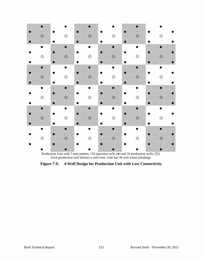
● ● ● ● ● ● ● ● ● ● ● ● ● ۞ ۞ ۞ ۞ ۞ ۞ ● ● ● ● ● ● ● ● ● ● ● ● ● ● ● ● ● ● ● ● ۞ ۞ ۞ ۞ ۞ ۞ ● ● ● ● ● ● ● ● ● ● ● ● ● ● ● ● ● ● ● ● ۞ ۞ ۞ ۞ ۞ ۞ ● ● ● ● ● ● ● ● ● ● ● ● ● ● ● ● ● ● ● ● ۞ ۞ ۞ ۞ ۞ ۞ ● ● ● ● ● ● ● ● ● ● ● ● ● ● ● ● ● ● ● ● ۞ ۞ ۞ ۞ ۞ ۞ ● ● ● ● ● ● ● ● ● ● ● ● ● ● ● ● ● ● ● ● ۞ ۞ ۞ ۞ ۞ ۞ ● ● ● ● ● ● ● ● ● ● ● ● ●
Production Unit with 7-spot pattern, 126 injection wells (●) and 36 production wells (۞). Each production well defines a well zone. Unit has 36 well zones (shading).
Figure 7-9. 4-Well Design for Production Unit with Low Connectivity
Draft Technical Report 153 Revised Draft – November 26, 2012

● ● ● ● ● ● ● ● ● ● ● ● ● ۞ ۞ ۞ ۞ ۞ ۞ ● ● ● ● ● ● ● ● ● ● ● ● ● ● ● ● ● ● ● ● ۞ ۞ ۞ ۞ ۞ ۞ ● ● ● ● ● ● ● ● ● ● ● ● ● ● ● ● ● ● ● ● ۞ ۞ ۞ ۞ ۞ ۞ ● ● ● ● ● ● ● ● ● ● ● ● ● ● ● ● ● ● ● ● ۞ ۞ ۞ ۞ ۞ ۞ ● ● ● ● ● ● ● ● ● ● ● ● ● ● ● ● ● ● ● ● ۞ ۞ ۞ ۞ ۞ ۞ ● ● ● ● ● ● ● ● ● ● ● ● ● ● ● ● ● ● ● ● ۞ ۞ ۞ ۞ ۞ ۞ ● ● ● ● ● ● ● ● ● ● ● ● ●
Production Unit with 7-spot pattern, 126 injection wells (●) and 36 production wells (۞). Unit has 16 well zones (shading) and an average zone contains 10 wells.
Figure 7-10. 10-Well Design for Production Unit with Good Connectivity
Draft Technical Report 154 Revised Draft – November 26, 2012

● ● ● ● ● ● ● ● ● ● ● ● ● ۞ ۞ ۞ ۞ ۞ ۞ ● ● ● ● ● ● ● ● ● ● ● ● ● ● ● ● ● ● ● ● ۞ ۞ ۞ ۞ ۞ ۞ ● ● ● ● ● ● ● ● ● ● ● ● ● ● ● ● ● ● ● ● ۞ ۞ ۞ ۞ ۞ ۞ ● ● ● ● ● ● ● ● ● ● ● ● ● ● ● ● ● ● ● ● ۞ ۞ ۞ ۞ ۞ ۞ ● ● ● ● ● ● ● ● ● ● ● ● ● ● ● ● ● ● ● ● ۞ ۞ ۞ ۞ ۞ ۞ ● ● ● ● ● ● ● ● ● ● ● ● ● ● ● ● ● ● ● ● ۞ ۞ ۞ ۞ ۞ ۞ ● ● ● ● ● ● ● ● ● ● ● ● ●
Production Unit with 7-spot pattern, 126 injection wells (●) and 36 production wells (۞). Unit has 9 well zones (shading) and an average zone contains 18 wells.
Figure 7-11. 18-Well Design for Production Unit with High Connectivity
Draft Technical Report 155 Revised Draft – November 26, 2012

Table 7-9. Ratio of Monitor Wells to Production Wells
Actual Number of Number of Number of Total
Site Production
Unit Ore Zone Monitor
Wells Extraction
Wells* Injection Wells*
Number of Wells
Highland Uranium Project A-Wellfield 5 38 48 86 Irigary Units 1 to 9 45 453 565 1,018 Christensen Ranch Units 2 to 5 78 663 838 1,501
44.2% 55.8% Crow Butte Unit 1 12 52 64 116 Totals 140 1,206 1,515 2,721 Averages 9.3 80.4 101 181.4
* Other sites estimated using Christensen Ranch proportion of injection/extraction wells
Table 7-10. Number of Monitoring Wells Required for Five Design Options for a Production Unit with 181 Wells in 5-spot Pattern (Posterior Probability=90%)
Posterior Probability=90% Percent of Well Zones Demonstrating Compliance (P) Number of Well
Design Option Zones P=70 75 80 85 90 91 92 93 94 95 96 97 98 99 2-Well Design 81 6 7 9 12 17 19 21 25 29 29 34 42 55 72 5-Well Design 36 5 7 8 10 15 15 18 18 18 24 24 24 32 32 7-Well Design 25 5 6 7 10 13 13 13 17 17 17 17 23 23 23
11-Well Design 16 5 5 6 8 11 11 11 11 15 15 15 15 15 15 20-Well Design 9 4 4 6 6 - - - - - - - - - -
Note: All clusters must be monitored.
Table 7-11. Number of Monitoring Wells Required for Five Design Options for a Production Unit with 181 Wells in 5-spot Pattern (Posterior Probability=95%)
Posterior Probability=95% Percent of Well Zones Demonstrating Compliance (P) Number of Well
Design Option Zones P=70 75 80 85 90 91 92 93 94 95 96 97 98 99 2-Well Design 81 7 9 11 15 21 24 27 30 35 35 41 50 62 76 5-Well Design 36 7 8 10 13 18 18 22 22 22 27 27 27 34 34 7-Well Design 25 6 7 9 12 15 15 15 19 19 19 19 24 24 24
11-Well Design 16 6 6 8 10 12 12 12 12 - - - - - - 20-Well Design 9 5 5 7 7 - - - - - - - - - -
Note: All clusters must be monitored.
Draft Technical Report 156 Revised Draft – November 26, 2012

Table 7-12. Number of Monitoring Wells Required for Four Design Options for a Production Unit with 162 Wells in 7-spot Pattern (Posterior Probability=90%)
Posterior Probability=90% Percent of Well Zones Demonstrating Compliance (P) Number of Well
Design Option Zones P=70 75 80 85 90 91 92 93 94 95 96 97 98 99 2-Well Design 72 5 7 9 12 16 19 21 25 25 30 37 37 48 63 4-Well Design 36 5 7 8 10 15 15 18 18 18 24 24 24 32 32
10-Well Design 16 5 5 6 8 11 11 11 11 15 15 15 15 15 15 18-Well Design 9 4 4 6 6 - - - - - - - - - -
Note: All clusters must be monitored.
Table 7-13. Number of Monitoring Wells Required for Four Design Options for a Production Unit with 162 Wells in 7-spot Pattern (Posterior Probability=95%)
Posterior Probability=95% Percent of Well Zones Demonstrating Compliance (P) Number of Well
Design Option Zones P=70 75 80 85 90 91 92 93 94 95 96 97 98 99 2-Well Design 72 7 9 11 15 21 23 26 31 31 36 44 44 54 67 4-Well Design 36 7 8 10 13 18 18 22 22 22 27 27 27 34 34
10-Well Design 16 6 6 8 10 12 12 12 12 - - - - - - 18-Well Design 9 5 5 7 7 - - - - - - - - - -
Note: All clusters must be monitored.
Draft Technical Report 157 Revised Draft – November 26, 2012

Table 7-14. Number of Monitoring Wells Required for Posterior Probability of 90% that at Least P% of the Well Zones Demonstrate Compliance
Number of Well Zones
Percent of Well Zones Demonstrating Compliance (P) P=70 75 80 85 90 91 92 93 94 95 96 97 98 99
5 3 3 3 - - - - - - - - - - - 6 4 4 4 - - - - - - - - - - - 7 3 5 5 5 - - - - - - - - - - 8 4 4 5 5 - - - - - - - - - - 9 4 4 6 6 - - - - - - - - - -
10 4 5 5 7 7 9 9 9 9 9 9 9 9 9 11 4 5 5 7 7 10 10 10 10 10 10 10 10 10 12 4 4 6 8 8 8 11 11 11 11 11 11 11 11 13 5 5 6 9 9 9 9 12 12 12 12 12 12 12 14 4 5 7 7 9 9 9 13 13 13 13 13 13 13 15 5 6 6 8 10 10 10 10 14 14 14 14 14 14 16 5 5 6 8 11 11 11 11 15 15 15 15 15 15 17 4 5 7 9 11 11 11 11 11 16 16 16 16 16 18 5 6 7 9 12 12 12 12 12 17 17 17 17 17 19 5 6 8 10 13 13 13 13 13 18 18 18 18 18 20 4 5 6 8 10 14 14 14 14 14 18 18 18 18 25 5 6 7 10 13 13 13 17 17 17 17 23 23 23 30 5 6 7 10 12 16 16 16 20 20 20 27 27 27 35 5 7 8 10 15 15 18 18 18 24 24 24 32 32 40 5 6 8 10 14 17 17 21 21 21 27 27 36 36 45 5 7 8 12 16 16 19 19 24 24 31 31 41 41 50 5 7 8 11 15 18 18 21 21 26 26 34 34 45 55 6 7 8 11 17 19 19 23 23 29 29 37 37 50 60 5 7 8 11 16 18 21 21 26 26 32 41 41 54 65 6 7 8 12 17 20 20 23 28 28 34 44 44 59 70 5 7 9 12 16 19 21 25 25 30 37 37 48 63 75 6 7 9 12 18 20 20 23 27 32 32 40 51 68 80 6 7 9 12 17 19 21 25 29 29 34 42 55 72 85 6 7 9 12 18 20 23 26 26 30 36 45 58 77 90 6 7 9 12 17 19 21 24 28 32 39 48 61 81 95 6 7 9 12 18 20 23 26 29 34 41 50 65 86
100 6 7 9 12 18 19 21 27 27 31 36 43 53 68 110 6 7 9 13 18 21 24 26 30 34 40 47 58 75 120 6 7 9 12 18 21 23 26 29 33 43 52 64 82 130 6 7 9 13 18 21 23 26 31 35 40 56 69 89 140 6 7 9 12 19 21 23 28 30 34 44 51 75 96 150 6 7 9 13 19 21 23 27 30 36 41 54 65 102 160 6 7 9 13 19 21 25 27 32 35 44 58 69 109 170 6 7 9 13 19 21 24 28 31 37 47 53 74 116 180 6 7 9 13 19 21 24 28 33 36 44 56 78 123 190 6 7 9 13 19 21 24 27 32 38 46 60 82 130 200 6 7 9 13 19 21 24 29 31 37 44 55 73 107
Draft Technical Report 158 Revised Draft – November 26, 2012

Table 7-14. Number of Monitoring Wells Required for Posterior Probability of 90% that at Least P% of the Well Zones Demonstrate Compliance
Number of Well Zones
Percent of Well Zones Demonstrating Compliance (P) P=70 75 80 85 90 91 92 93 94 95 96 97 98 99
225 6 7 9 13 20 22 24 29 33 38 45 62 82 120 250 6 7 9 13 20 22 25 29 32 39 46 61 79 133 300 6 7 9 13 20 22 25 30 33 39 47 60 83 131 350 6 7 10 13 20 23 25 29 33 41 48 65 86 152 400 6 7 10 13 20 23 25 30 34 40 49 64 89 147 450 6 7 10 13 20 23 26 30 34 41 50 67 91 165 500 6 7 10 13 20 23 26 30 34 41 50 66 93 158 600 6 7 10 13 21 23 26 30 35 41 51 67 96 167 700 6 7 10 13 21 23 26 31 35 42 52 68 98 174 800 6 7 10 13 21 23 26 31 35 42 52 69 100 179 900 6 7 10 13 21 23 26 31 35 42 53 70 101 184
1000 6 7 10 13 21 23 26 31 35 43 53 70 102 188 Note: All clusters
must be monitored.
Table 7-15. Number of Monitoring Wells Required for Posterior Probability of 95% that at Least P% of the Well Zones Demonstrate Compliance
Number of Well Zones
Percent of Well Zones Demonstrating Compliance (P) P=70 75 80 85 90 91 92 93 94 95 96 97 98 99
5 4 4 4 - - - - - - - - - - - 6 4 4 4 - - - - - - - - - - - 7 4 5 5 5 - - - - - - - - - - 8 4 4 6 6 - - - - - - - - - - 9 5 5 7 7 - - - - - - - - - -
10 4 6 6 8 8 - - - - - - - - - 11 5 6 6 8 8 - - - - - - - - - 12 5 5 7 9 9 9 - - - - - - - - 13 6 6 8 10 10 10 10 - - - - - - - 14 5 7 8 8 11 11 11 - - - - - - - 15 6 7 7 9 12 12 12 12 - - - - - - 16 6 6 8 10 12 12 12 12 - - - - - - 17 5 7 8 10 13 13 13 13 13 - - - - - 18 6 7 9 11 14 14 14 14 14 - - - - - 19 6 8 9 11 15 15 15 15 15 - - - - - 20 6 7 8 10 12 15 15 15 15 15 19 19 19 19 25 6 7 9 12 15 15 15 19 19 19 19 24 24 24 30 6 8 9 13 15 18 18 18 23 23 23 29 29 29 35 7 8 10 13 18 18 22 22 22 27 27 27 34 34 40 7 8 10 13 17 20 20 25 25 25 31 31 38 38 45 7 8 10 14 19 19 23 23 28 28 35 35 43 43 50 7 9 10 14 19 22 22 26 26 31 31 39 39 48 55 7 9 11 14 20 24 24 28 28 34 34 43 43 53
Draft Technical Report 159 Revised Draft – November 26, 2012

Table 7-15. Number of Monitoring Wells Required for Posterior Probability of 95% that at Least P% of the Well Zones Demonstrate Compliance
Number of Well Zones
Percent of Well Zones Demonstrating Compliance (P) P=70 75 80 85 90 91 92 93 94 95 96 97 98 99
60 65 70 75 80 85 90 95
100 110 120 130 140 150 160 170 180 190 200 225 250 300 350 400 450 500 600 700 800 900
1000
7 7 7 7 7 7 7 7 7 7 7 7 7 8 8 8 8 8 8 8 8 8 8 8 8 8 8 8 8 8 8
9 9 9 9 9 9 9 9 9 9 9 9 9 9 9
10 9
10 9
10 10 10 10 10 10 10 10 10 10 10 10
11 11 11 11 11 11 11 11 12 12 12 12 12 12 12 12 12 12 12 12 12 12 12 13 13 13 13 13 13 13 13
14 15 15 15 15 16 16 16 15 16 16 16 16 17 16 17 16 17 17 17 17 17 17 17 17 17 17 18 18 18 18
20 21 21 22 21 23 22 23 22 23 23 23 24 24 24 24 25 25 25 26 25 26 26 26 26 27 27 27 27 27 27
22 24 23 25 24 25 24 26 24 27 27 27 27 27 27 27 27 27 27 28 29 29 29 29 30 30 30 30 30 30 30
26 24 26 25 27 28 27 28 27 30 30 30 29 29 31 31 31 31 31 31 32 32 33 33 33 33 34 34 34 34 34
26 28 31 28 30 32 30 32 34 33 33 32 35 34 34 36 35 35 37 37 37 38 38 39 38 39 39 40 40 40 40
31 33 31 33 35 32 34 36 34 37 36 39 38 37 40 39 41 40 40 42 41 42 43 43 44 44 45 45 46 46 46
31 33 36 39 35 37 40 42 38 42 41 44 42 46 44 47 45 48 46 48 50 50 52 51 53 53 53 54 55 55 55
37 41 44 39 41 44 47 49 44 49 53 50 54 51 54 58 55 58 55 57 58 60 62 63 64 65 66 67 68 68 69
46 50 44 47 50 53 56 59 52 57 62 68 62 67 71 66 70 74 68 77 77 76 82 81 85 84 86 87 89 90 90
46 50 54 58 62 66 70 74 63 69 75 82 88 78 84 89 94 99 89
100 97
103 108 112 115 118 122 125 128 130 131
57 62 67 72 76 81 86 91 78 85 93
101 109 116 124 132 140 147 126 142 157 157 184 179 202 195 208 217 225 232 237
Note: All clusters must be monitored.
7.2.3 Determining Connectivity of the Wellfield
Connectivity of the wellfield may be measured using both physical and statistical methods. An example of a physical measure of connectivity is the hydraulic conductivity of the ground water. Connectivity may also be demonstrated based on an analysis of the spatial correlation between measurements in nearby wells. Spatial autocorrelation is a generalization of one-dimensional temporal autocorrelation. Spatial correlation may be defined in two, three or more dimensions. In this application two-dimensional spatial autocorrelation is of interest. In two or more dimensions autocorrelation is multi-directional.
Draft Technical Report 160 Revised Draft – November 26, 2012

Two- and three-dimensional data with spatial correlation are best analyzed using geostatistical methods. Geostatistics is capable of using the information revealed by a correlation analysis of the data to estimate concentrations at unsampled locations and in areas where data are sparse. Although application of these methods often requires specialized software and skilled practitioners, operators are encouraged to perform geostatistical analysis to obtain a better understanding of the site. Geostatistical analysis may reveal anomalous baseline conditions in certain areas of the site or areas where remediation has not been successful. A full discussion of geostatistics is beyond the scope of this document. Some examples of the application of geostatistics in the analysis of ground water contamination can be found in Chapter 6 of EPA 2000b. Moran's I statistic is one measure of spatial association that does not require specialized software. This statistic is a global measure of spatial autocorrelation characterized by a correlation among nearby wells. In addition to the data from each well, Moran’s I statistic requires matrix of spatial weights. In the most elementary case, the weight matrix may be derived from a distance matrix. The distance matrix has elements that represent the “distance” between well i and well j. The distance matrix may be expressed in physical units of length, or may contain other measures of distance, such as the travel time between wells. The weight matrix for the I statistic has elements equal to the inverse of the elements of the distance matrix. The weight matrix measures the “nearness” of each well to the other wells. The weighting entries for pairs of wells that are close together are higher than for pairs of wells that are far apart. The weight matrix has off-diagonal entries wi, j equal to 1 divided by the distance between well i and well j. The diagonal entries of the weight matrix are set to 0. This is one of several ways to calculate an inverse distance matrix. For example, the inverse distance matrix may have off-diagonal entries equal to 1 divided by 1 plus the distance between well i and well j. Moran's I is calculated using the formula:
( )( )( )
−
−−⋅
=
∑∑∑
∑∑ i i
i j jiji
i j ji XX
XXXXw
wNI 2
,
,
where N is the number of spatial units indexed by i, j=1, …, N; X is the analyte of interest; X is the mean of X; and wi,j is an element of the spatial weight matrix. The expected value of Moran's I statistic under a hypothesis of no spatial autocorrelation is E(I ) = −1 (N −1) . Positive (negative) values of I indicate positive (negative) spatial autocorrelation. Values of I range from −1, indicating perfect dispersion, to +1, indicating perfect correlation between the wells. A zero value indicates a random spatial pattern. For statistical hypothesis testing, Moran's I values can be transformed to normal scores in which values greater than 1.96 (or smaller than −1.96) indicate spatial autocorrelation that is significant at the 5% level.
Draft Technical Report 161 Revised Draft – November 26, 2012
7.3 Hypothesis Testing and Data Quality Objectives
Hypothesis testing is a statistical tool for deciding when the ground water has reached steady state and for comparing post-restoration conditions with baseline conditions. The hypothesis tests are conducted for individual wells and, when wells exhibit homogeneous dynamics, for all wells combined.
The first step in developing a hypothesis test is to transform the problem into statistical terminology by formulating a null hypothesis and an alternative hypothesis. These hypotheses form the two alternative decisions that the hypothesis test will evaluate. When a well is compared with the baseline, the unknown parameter of interest (δ) is the amount by which the post-restoration distribution exceeds the baseline distribution (See Box 7-1). Delta (δ) is an unknown value, and statistical tests may be used to evaluate hypotheses relating to its possible values. A hypothesis test is designed to reject or not reject hypotheses about δ based on test statistics computed from the sample data. At its core, this is another example of the “How clean is clean?” problem. The action level for baseline comparisons is the largest difference in the two distributions that is acceptable to the decision maker. In this report, the action level for this difference is defined as a substantial difference (Δ), which may be zero or a positive value based on the risk assessment, an applicable regulation, a screening level, or guidance.
This document does not establish a specific value for a substantial difference Δ, as the value will vary from parameter to parameter and from site to site. Therefore, specific values for Δ should be considered on a case-by-case basis. In many cases, the minimum feasible value of Δ is determined by the usual variability in that parameter during the pre-leaching phase (Phase 1 in Figure 3-1). Appendix A to EPA 2002a discusses further the selection of a value for Δ. The determination of Δ for each parameter of interest should be considered during the development of a quality assurance project plan as part of the planning process for the site evaluation. Hypothesis testing is a quantitative method to determine whether a specific statement concerning the unknown difference δ (a statement known as the “null hypothesis”) can be rejected based on the data at hand. Decisions concerning the true value of δ (e.g., is δ > 0?) reduce to a choice of “yes” or “no.” When viewed in this way, two types of incorrect decisions, or decision errors, may occur:
• Incorrectly deciding the answer is “yes” when the true answer is “no” • Incorrectly deciding the answer is “no” when the true answer is “yes”
While the possibility of decision errors can never be totally eliminated, it can be controlled to acceptable levels. To control decision errors, it is necessary to control the uncertainty in the estimate of δ. Uncertainty arises from three sources:
• Sampling error • Measurement error • Natural variability
Draft Technical Report 162 Revised Draft – November 26, 2012

The decisionmaker has some control over the first two sources of uncertainty. For example, a larger number of samples may lead to fewer decision errors because the probability of a decision error decreases as the number of samples increases. Use of more precise measurement techniques or duplicate measurements can reduce measurement error, thus minimizing the likelihood of a decision error. The third source of uncertainty is more difficult to control. Natural variability arises from the uneven distribution of chemical concentrations and conditions at the site.
Natural variability includes both spatial and temporal variability. When measurements are made in different wells over a relatively short period of time, spatial variability is measured by the standard deviation (σ) of the measurements around their mean value. A large value of σ indicates that a large number of measurements will be needed to achieve a desired limit on decision errors. Baseline samples may have a different variability than post-restoration samples. As post-restoration variability is usually higher than in the baseline, post-restoration data ideally would be used to estimate σ.
Temporal variability measures the variability of concentration in a well over time. Short-term variability may be random or have a seasonality pattern. Long-term temporal variability may appear as a trend. In the case of a trend, temporal variability is defined in terms of the variation of the measurements from the trendline.
It is advisable to overestimate σ rather than underestimate the true variability. A very crude approximation for σ may be made by dividing the anticipated range (maximum minus minimum) by 6 (EPA 2002a, Section 3.1). It is important that overly optimistic estimates for σ be avoided, because this may result in a sample size that fails to generate sufficient data to distiguish between the null and alternative hypotheses. In statistical terms, the test will lack sufficient power if the sample size is too small. The power of a statistical hypothesis test is discussed in the following section.
The minimum detectable difference (MDD) for a statistical test indicates that differences smaller than the MDD cannot be detected reliably. If the test is used to decide if post-restoration concentrations exceed the baseline concentrations by more than Δ, it is necessary to ensure that the MDD for the test is less than Δ. In the planning stage, this requirement is met by designing a sampling plan with sufficient power to detect differences as small as Δ (MDD ≤ Δ). If data were collected without the benefit of a sampling plan, retrospective calculation of the power of the test may be necessary before making a decision.
In the planning stage, the absolute size of the MDD is of less importance than the ratio of the MDD to the natural variability of the post-restoration concentrations. This ratio is termed the relative difference and is defined as MDD/σ, where σ is an estimate of the standard deviation of the post-restoration distribution. The relative difference expresses the power of resolution of the statistical test (MDD) in units of uncertainty (σ). Relative differences much less than 1 standard deviation (MDD/σ << 1) are more difficult to resolve unless a larger number of measurements are available. Relative differences of more than 3 standard deviations (MDD/σ > 3) are easier to resolve.
Draft Technical Report 163 Revised Draft – November 26, 2012
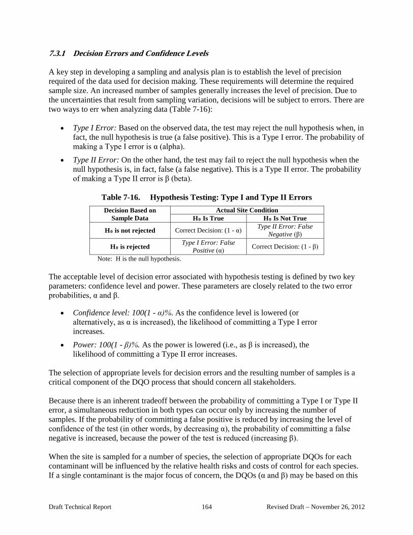
7.3.1 Decision Errors and Confidence Levels
A key step in developing a sampling and analysis plan is to establish the level of precision required of the data used for decision making. These requirements will determine the required sample size. An increased number of samples generally increases the level of precision. Due to the uncertainties that result from sampling variation, decisions will be subject to errors. There are two ways to err when analyzing data (Table 7-16):
• Type I Error: Based on the observed data, the test may reject the null hypothesis when, in fact, the null hypothesis is true (a false positive). This is a Type I error. The probability of making a Type I error is α (alpha).
• Type II Error: On the other hand, the test may fail to reject the null hypothesis when the null hypothesis is, in fact, false (a false negative). This is a Type II error. The probability of making a Type II error is β (beta).
Table 7-16. Hypothesis Testing: Type I and Type II Errors Decision Based on Actual Site Condition
Sample Data H0 Is True H0 Is Not True Type II Error: False H0 is not rejected Correct Decision: (1 - α) Negative (β)
Type I Error: False H0 is rejected Correct Decision: (1 - β) Positive (α) Note: H is the null hypothesis.
The acceptable level of decision error associated with hypothesis testing is defined by two key parameters: confidence level and power. These parameters are closely related to the two error probabilities, α and β.
• Confidence level: 100(1 - α)%. As the confidence level is lowered (or alternatively, as α is increased), the likelihood of committing a Type I error increases.
• Power: 100(1 - β)%. As the power is lowered (i.e., as β is increased), the likelihood of committing a Type II error increases.
The selection of appropriate levels for decision errors and the resulting number of samples is a critical component of the DQO process that should concern all stakeholders. Because there is an inherent tradeoff between the probability of committing a Type I or Type II error, a simultaneous reduction in both types can occur only by increasing the number of samples. If the probability of committing a false positive is reduced by increasing the level of confidence of the test (in other words, by decreasing α), the probability of committing a false negative is increased, because the power of the test is reduced (increasing β). When the site is sampled for a number of species, the selection of appropriate DQOs for each contaminant will be influenced by the relative health risks and costs of control for each species. If a single contaminant is the major focus of concern, the DQOs (α and β) may be based on this
Draft Technical Report 164 Revised Draft – November 26, 2012
species. If more than one species is a matter of concern, the Bonferroni correction19 is a simple approach for addressing the problem. If the species are of equal concern, the nominal significance level for each test (α) is divided by the number of contaminants that are to be tested. Similarly, when the species have different levels of concern, adjustments may be made using a different α for each species. However, the sample size calculations (described below) show that this reduction in the significance level requires a major increase in the amount of data to be collected. The issue of multiple comparisons is beyond the intended scope of this document. A complete discussion of Bonferroni confidence intervals and newer alternative approaches to the multiple-comparison problem is presented in Bickel and Doksum (2006). In terms of not exceeding the regulatory limits, we believe the confidence level for decisions involving the listed radionuclides should be equivalent. The limits for other analytes may be less stringent but still consistent with the value of the parameter in making a safety case.
7.3.2 Hypothesis Tests for Comparisons with Baseline
Statistical hypothesis tests are used for comparing post-restoration conditions with baseline conditions and for demonstrating stability of the site after restoration. Three statistical methods are presented for the comparison with baseline conditions. The two-sample t-test and prediction limits for a future mean are two parametric methods used in the comparison with baseline conditions. Prediction limits (PLs) are designed to provide an upper bound for the mean of a future sample with a specified probability equal to (1 - α), known as the confidence level of the PL. It represents the chance that the PL will contain the mean of a future (post-operations) sample from the monitoring wells. The nonparametric WRS test is also used to compare post-restoration well conditions with baseline values. This test compares the relative ranks of the two data sets. The two-sample t-test and the WRS test are recommended for comparing baseline and post-remedial wells (EPA 2006a). The RCRA Unified Guidance (EPA 2009) recommends the PL method. The three different statistical tests for comparisons with baseline conditions are used in Phase 4 to determine if the restoration goals have been met. A choice of one of the three different statistical tests should be made before post-restoration data are collected. The selected test procedure is then applied for all wells. The prior selection of a single testing approach is necessary for comparability of results across wells and to avoid the possibility of running all three tests, then selecting the test with most favorable results.
Two forms of hypothesis tests are used for comparisons with baseline conditions. The null hypothesis in the first form of the test (Test Form 1) states that there is no statistically significant difference between the means of the baseline and post-restoration concentration distributions. The null hypothesis in the second form of the test (Test Form 2) states that the post-restoration mean exceeds the baseline mean by more than a substantial difference Δ. Either test form may be used with the two-sample t-test and the WRS test. Test Form 1 is used for PLs.
19 The Bonferroni correction is a statistical method used to address the problem of multiple comparisons. It helps control the probability of Type I errors (i.e., false positives).
Draft Technical Report 165 Revised Draft – November 26, 2012

Test Form 1
The null hypothesis for Test Form 1 is formulated for the express purpose of being rejected when restoration has not been successful. If the null hypothesis is rejected, the alternative hypothesis is accepted, indicating that baseline conditions have not been achieved.
• The null hypothesis (H0): The mean of the post-restoration distribution does not exceed the baseline mean. Symbolically, the null hypothesis for Test Form 1 is H0: δ ≤ 0.
• The alternative hypothesis (HA): The post-restoration distribution mean exceeds the baseline mean: (HA: δ > 0).
When using Test Form 1, the null hypothesis is presumed true until it is rejected. A problem may arise in the use of Test Form 1 when insufficient data are available for the decision. If insufficient data are available, Test Form 1 may lead to inconclusive results due to a lack of power. Figure 7-12 illustrates an example of a test performance plot for Test Form 1. At the origin of the plot, the true difference between the means of the two distributions is zero. Positive values of the difference are plotted on the horizontal axis to the right of the origin, negative values to the left. The vertical axis shows the probability of rejecting the null hypothesis, which for this test form is the probability of deciding the post-restoration mean concentration exceeds the mean baseline concentration. This probability ranges from 0 to 1.0 (0% to 100%). The gray region for the test extends from 0 up to the MDD. It is necessary to specify a gray region for the test, because the decision may be “too close to call” due to uncertainty. This may occur when the difference in means is small compared to the MDD for the test. To the left or right of the gray region, the test outcome is easy to determine. In the gray region, the statistical test has difficulty deciding between the two alternatives. To the left of the gray region, the test performance curve is no greater than α. In the gray region, the test performance curve increases as the difference between the means increases. The number of samples and the standard deviation, σ, determine the rate of increase. The right edge of the gray region is located at the MDD. The MDD measures the width of the gray region for the test. When the difference between the means is equal to the MDD, the probability of deciding that the post-restoration mean exceeds the baseline mean is equal to the power of the test (1 –β).
Figure 7-12 also shows a hypothetical value of a substantial difference for this analyte of Δ = 100. This value is used in the DQO process as an upper limit for the width of the gray region (MDD). In this example, an MDD less than Δ was selected for the test. If the MDD is selected to be smaller than Δ, then differences from baseline smaller than Δ can be detected by the test with a high probability.
Draft Technical Report 166 Revised Draft – November 26, 2012
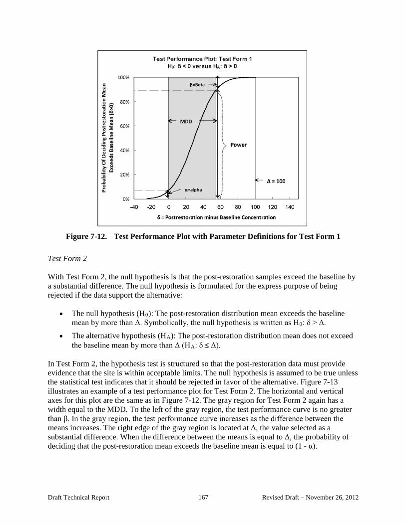
Figure 7-12. Test Performance Plot with Parameter Definitions for Test Form 1
Test Form 2
With Test Form 2, the null hypothesis is that the post-restoration samples exceed the baseline by a substantial difference. The null hypothesis is formulated for the express purpose of being rejected if the data support the alternative:
• The null hypothesis (H0): The post-restoration distribution mean exceeds the baseline mean by more than Δ. Symbolically, the null hypothesis is written as H0: δ > Δ.
• The alternative hypothesis (HA): The post-restoration distribution mean does not exceed the baseline mean by more than Δ (HA: δ ≤ Δ).
In Test Form 2, the hypothesis test is structured so that the post-restoration data must provide evidence that the site is within acceptable limits. The null hypothesis is assumed to be true unless the statistical test indicates that it should be rejected in favor of the alternative. Figure 7-13 illustrates an example of a test performance plot for Test Form 2. The horizontal and vertical axes for this plot are the same as in Figure 7-12. The gray region for Test Form 2 again has a width equal to the MDD. To the left of the gray region, the test performance curve is no greater than β. In the gray region, the test performance curve increases as the difference between the means increases. The right edge of the gray region is located at Δ, the value selected as a substantial difference. When the difference between the means is equal to Δ, the probability of deciding that the post-restoration mean exceeds the baseline mean is equal to (1 - α).
Draft Technical Report 167 Revised Draft – November 26, 2012

An MDD less than Δ was selected for the test. If the MDD is selected to be smaller than Δ, then the test will have greater power to accept sites when the difference in means is less than Δ.
Figure 7-13. Test Performance Plot with Parameter Definitions for Test Form 2
7.3.3 Selecting a Test Form
When comparing Test Forms 1 and 2, it is important to distinguish between the selection of the null hypothesis, which is a burden-of-proof issue, and the selection of the substantial difference, which involves determination of an action level. Test Form 1 uses a conservative level of 0 as the maximum acceptable difference, but relaxes the burden of proof by selecting a null hypothesis that the post-restoration mean is not statistically different from the baseline mean. Test Form 2 requires a stricter burden of proof, but relaxes the action level from 0 to Δ. See Box 7.2 for more information on the parameters of Test Form 1 and Test Form 2. EPA2002a and MARSSIM (EPA 2000a) include further discussion of how to choose between Test Forms 1 and 2 (MARSSIM uses the terms Scenario A and Scenario B for Test Forms 2 and 1, respectively), and provide additional guidance for setting up the hypotheses. Regardless of the choice of hypothesis for the comparison with baseline conditions, an incorrect conclusion could be drawn from the data analysis using either form of test. To account for this inherent uncertainty, one should specify the limits on the decision errors. This task was described in Section 7.3.1. The selection of a null hypothesis depends on what the “working assumption” is for each monitoring phase and, perhaps more generally, what has already occurred. For post-restoration, one “assumes the worst,” i.e., that post-restoration values exceed the baseline by more than Δ. Compliance can be demonstrated only by collecting sufficient data to reject the null hypothesis
Draft Technical Report 168 Revised Draft – November 26, 2012

(i.e., “proving” the alternative). For this phase, a regulator would be primarily concerned with the occurrence of Type I errors (showing compliance when not justified). However, when using a trend test to demonstrate that the site is stable, the null hypothesis would be a statement of no trend. The null hypothesis would stand until sufficient data show evidence of a trend.
A Type 2 error occurs if the null hypothesis is accepted when it is not true. With Test Form 1, a Type 1 error occurs when the site is incorrectly determined to require further restoration. A Type 2 error means that the site was incorrectly determined to be in compliance. From a human health perspective, a Type 2 error is more serious than a Type 1 error. Hence, it is reasonable that the Type 2 error rate (β) should be smaller than the Type 1 error rate (α). Using Test Form 1, the regulator would be concerned with Type 2 errors, and the specification of MDDs and minimum sample sizes will be of particular importance to the regulator.20
With Test Form 2, a Type 1 error occurs when the site is incorrectly determined to be in compliance. A Type 2 error means that the site was incorrectly determined to require further restoration. From a human health perspective, a Type 1 error is more serious than a Type 2 error. In this case, it is reasonable that the Type 1 error rate (α) should be smaller than the Type 2 error rate (β). Once α is selected, a higher value of β will reduce the required number of samples, but there will be a greater likelihood that the site is incorrectly determined to be out of compliance. In this case, the site operator faces a trade-off and may select to reduce the value of β (at the expense of a greater number of samples) and increase the power of the test in order to avoid the possibility of Type 2 errors.
For the purposes of this report, the minimum recommended performance measures are:
Test Form 1: Confidence level at least 80% (α ≤ 0.20) and power at least 90% (β ≤ 0.10)
Test Form 2: Confidence level at least 90% (α ≤ 0.10) and power at least 80% (β ≤ 0.20). (EPA 2002a, Section 3.2)
Box 7-2 describes these performance standards in more detail.
20 Documents such as EPA (2009) describe processes involving several phases, and the null hypothesis depends on the phase of the process and/or what may have occurred previously. For some stages, the null hypothesis would be a statement that “all is well” (e.g., there is no trend for a particular contaminant at a particular well monitoring location). For other stages, the null hypothesis is just the opposite (e.g., the site is out of compliance with respect to a particular contaminant). For the former case, rejection of the null hypothesis in effect “proves” that the site is not stable, and regulators would be primarily concerned with the occurrence of what statisticians refer to as Type 2 errors (we are unable to detect a worrisome trend when such a trend exists). For the latter, the primary concern would be the occurrence of a Type I error (falsely concluding that the site is in compliance when it is not).
Draft Technical Report 169 Revised Draft – November 26, 2012

Box 7-1. Definitions
δ (delta): The true difference between the post-restoration distribution and the baseline distribution of parameter X. Delta is an unknown value that describes the true state of nature. Hypotheses about its value are evaluated using statistical hypothesis tests. In principle, we can select any specific value for δ and then test if this difference is statistically significant or not with a given confidence and power. Δ (a substantial difference): A difference between the two distributions that is sufficiently large to warrant additional interest based on health or ecological information. Δ is the investigation level. If δ exceeds Δ, the difference in concentrations is judged to be sufficiently large to be of concern for the purpose of the analysis. A hypothesis test uses baseline and post-restoration measurements to determine if δ exceeds Δ. MDD (minimum detectable difference): The smallest difference that the statistical test can resolve. The MDD depends on sample-to-sample variability, the number of samples, and the power of the statistical test. The MDD is a property of the survey design.
Box 7-2. Interpretation of the Statistical Measures for Test Forms 1 and 2
Test Form 1 Confidence level = 80%: On average, in 80 out of 100 cases, post-restoration concentrations are correctly identified as not exceeding baseline concentrations by more than Δ, while in 20 out of 100 cases, post-restoration concentrations will be incorrectly identified as exceeding baseline concentrations by more than Δ when, in fact, they do not. For a confidence level of 80%, choose α=0.20. Power = 90%: On average, in 90 out of 100 cases, post-restoration concentrations will be correctly identified as exceeding baseline concentrations by more than Δ, while in 10 out of 100 cases, post-restoration concentrations will be incorrectly identified as not exceeding baseline concentrations by more than Δ when, in fact, they do. For power of 90%, choose β=0.10.
Test Form 2
Confidence level = 90%: On average, in 90 out of 100 cases, post-restoration concentrations are correctly identified as exceeding baseline concentrations by more than Δ, while in 10 out of 100 cases, post-restoration concentrations will be incorrectly identified as not exceeding baseline concentrations by more than Δ when, in fact, they do. For a confidence level of 90%, choose α=0.10. Power = 80%: On average, in 80 out of 100 cases, post-restoration concentrations will be correctly identified as not exceeding baseline concentrations by more than Δ, while in 20 out of 100 cases, post-restoration concentrations will be incorrectly identified as exceeding baseline concentrations by more than Δ when, in fact, they do not. For power of 80%, choose β=0.20.
7.3.4 Hypothesis Tests for Detecting Trends
Two statistical tests for trends are used for stability monitoring in Phase 5, a parametric trend test based on the linear regression model and the nonparametric Mann-Kendall trend test. A choice of one these statistical tests should be made before stability monitoring is begun. The selected
Draft Technical Report 170 Revised Draft – November 26, 2012

test procedure is then applied for all monitored wells. Selection of a single testing approach is necessary for comparability of results across wells and to avoid the possibility of running both tests, then selecting the test with most favorable results. Linear regression and the nonparametric Mann-Kendall trend test are recommended for trend detection in EPA 2006a and EPA 2009. The linear regression trend test relies on a variety of assumptions (e.g., normality) that must be verified. The Mann-Kendall trend test may be used with any series of four or more independent samples to test for trends in well parameters. Trend tests are used in Phase 1 to check for unexpected trends in baseline samples, and in Phase 5 to establish long-term stability. Test Form 1 is used for the regression t-test and the Mann-Kendall trend test. In regression, a trend is measured by the slope of the regression line θ (theta). Here θ represents the true (and unknowable) value of the slope of the trend line. In the Mann-Kendall test, a trend is charactered by the parameter τ (tau), which is a nonparametric measure of the correlation of the sample values with time. In each case, hypothesis tests are used to determine if there is a significant trend over time. The null hypothesis for both tests is that there is no trend. The time series is analyzed for evidence of a significant trend. If such evidence is found, then the null hypothesis is rejected. Testing for a trend:
• The null hypothesis (H0): There is no significant trend in the series. Symbolically, the null hypothesis for the trend test is H0: θ=0.
• The alternative hypothesis (HA): There is a significant trend in the series. (HA: θ ≠ 0). The null and alternative hypotheses for the Mann-Kendall test are similar, with θ being replaced by τ. Unlike the tests for a comparison with baseline conditions, the trend tests require only one DQO parameter, the Type 1 error rate α. This parameter provides a control on the frequency of false positives, i.e., incorrectly deciding there is a trend when, in fact, the series is stationary. The power (1-β) of the trend tests to detect a trend depends on the variability of the series, the type of trend, duration of the sampling program and the frequency of sampling. The power of these tests may be estimated using Monte Carlo simulation. The power of the rank-based Mann-Kendal test and the linear regression t-test for slope are compared by Yue and Pilon (2004), who report that the power of the t-test is slightly higher than that of the Mann-Kendall test for normally distributed data, and for nonnormally distributed series, such as time series with the Weibull, Gumbel, Pearson Type III, or extreme value Type II distributions, the power of the Mann-Kendall test is higher than that of the t-test. The t-test usually performs better with a distribution that is relatively symmetric. In contrast, the Mann-Kendall is a more powerful test for data sets that present skewness. Attachment G contains a detailed discussion of the simulations performed for this study to determine a sufficient number of samples to provide adequate power to detect trends.
Draft Technical Report 171 Revised Draft – November 26, 2012
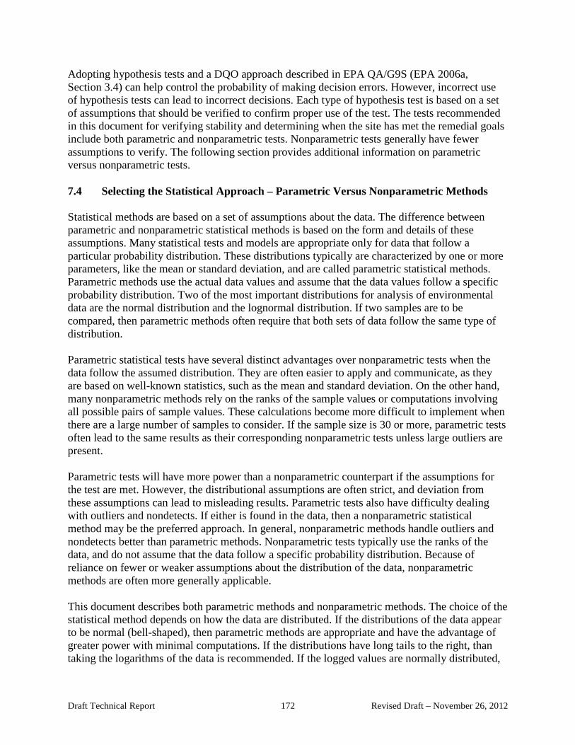
Adopting hypothesis tests and a DQO approach described in EPA QA/G9S (EPA 2006a, Section 3.4) can help control the probability of making decision errors. However, incorrect use of hypothesis tests can lead to incorrect decisions. Each type of hypothesis test is based on a set of assumptions that should be verified to confirm proper use of the test. The tests recommended in this document for verifying stability and determining when the site has met the remedial goals include both parametric and nonparametric tests. Nonparametric tests generally have fewer assumptions to verify. The following section provides additional information on parametric versus nonparametric tests.
7.4 Selecting the Statistical Approach – Parametric Versus Nonparametric Methods
Statistical methods are based on a set of assumptions about the data. The difference between parametric and nonparametric statistical methods is based on the form and details of these assumptions. Many statistical tests and models are appropriate only for data that follow a particular probability distribution. These distributions typically are characterized by one or more parameters, like the mean or standard deviation, and are called parametric statistical methods. Parametric methods use the actual data values and assume that the data values follow a specific probability distribution. Two of the most important distributions for analysis of environmental data are the normal distribution and the lognormal distribution. If two samples are to be compared, then parametric methods often require that both sets of data follow the same type of distribution.
Parametric statistical tests have several distinct advantages over nonparametric tests when the data follow the assumed distribution. They are often easier to apply and communicate, as they are based on well-known statistics, such as the mean and standard deviation. On the other hand, many nonparametric methods rely on the ranks of the sample values or computations involving all possible pairs of sample values. These calculations become more difficult to implement when there are a large number of samples to consider. If the sample size is 30 or more, parametric tests often lead to the same results as their corresponding nonparametric tests unless large outliers are present.
Parametric tests will have more power than a nonparametric counterpart if the assumptions for the test are met. However, the distributional assumptions are often strict, and deviation from these assumptions can lead to misleading results. Parametric tests also have difficulty dealing with outliers and nondetects. If either is found in the data, then a nonparametric statistical method may be the preferred approach. In general, nonparametric methods handle outliers and nondetects better than parametric methods. Nonparametric tests typically use the ranks of the data, and do not assume that the data follow a specific probability distribution. Because of reliance on fewer or weaker assumptions about the distribution of the data, nonparametric methods are often more generally applicable.
This document describes both parametric methods and nonparametric methods. The choice of the statistical method depends on how the data are distributed. If the distributions of the data appear to be normal (bell-shaped), then parametric methods are appropriate and have the advantage of greater power with minimal computations. If the distributions have long tails to the right, than taking the logarithms of the data is recommended. If the logged values are normally distributed,
Draft Technical Report 172 Revised Draft – November 26, 2012

then parametric methods may be applied to the logged data. If both data sets cannot be determined to have normal (or lognormal) distributions, then nonparametric methods might be appropriate.
7.4.1 Determining If Data Have a Normal Distribution
Many statistical tests and models are appropriate only for data that follow a particular distribution. Methods in this section apply to the normal distribution. The tests for normality also may be used with lognormal data by applying the prescribed test to the logarithms of the data. If the data appear to have a distribution other than the normal distribution or the lognormal distribution, a nonparametric test such as the Wilcoxon Rank Sum test (see Section 7.9.2) should be considered.
7.4.2 The Shapiro-Wilk W Test
The Shapiro-Wilk W test is considered one of the most powerful tests for normality. This test is similar to computing a correlation between the quantiles of the standard normal distribution and the ordered values of a data set. Several EPA guidance documents and many statistical texts recommend the W test. Tables of critical values for sample sizes up to 50 have been developed for determining the significance of the test statistic. However, many software packages can perform the W test for data sets with sample sizes as large as 5,000. This test is difficult to compute by hand as it requires many summations and multiplications. Therefore, this document does not give directions for implementing the W test. The Studentized Range test described below is another test for normality that is much easier to compute, but is not as powerful as the W test.
7.4.3 The Studentized Range Test
The Studentized Range test for normality is based on the fact that nearly 100% of the area of a normal curve lies within ±5 standard deviations from the mean. This test uses a ratio of the sample range to the sample standard deviation. Very large and very small values of the ratio imply that the data are not well modeled by a normal distribution
This test for normality compares the sample range (maximum value minus minimum value) to the sample standard deviation. The test statistic is the ratio of the sample range to the standard deviation. Table 7-17 shows the critical values for determining whether the absolute value of the ratio for a sample of size N is significantly too small or too large. If the calculated ratio is less than the lower tabulated value (a) or exceeds the upper value (b), then the data are not normally distributed at the specified level of confidence. The Studentized Range test does not perform well if the data are asymmetric or if the tails of the data are heavier than the normal distribution. In addition, this test may be sensitive to a few extreme values. The test for outliers described in the following section may be used to screen the data for outliers before the Studentized Range test is conducted.
Many environmental data sets are positively skewed with a long but narrow tail of high values and are similar to a lognormal distribution. If the data appear to be lognormally distributed, then the range test may be applied to the logged data values.
Draft Technical Report 173 Revised Draft – November 26, 2012
Table 7-17. Critical Values for the Studentized Range Test
Confidence Level 90% 95% 99%
N a b a b a b 3 1.78 2.00 1.76 2.00 1.74 2.00 4 2.04 2.41 1.98 2.43 1.87 2.45 5 2.22 2.71 2.15 2.75 2.02 2.80 6 2.37 2.95 2.28 3.01 2.15 3.10 7 2.49 3.14 2.40 3.22 2.26 3.34 8 2.59 3.31 2.50 3.40 2.35 3.54 9 2.68 3.45 2.59 3.55 2.44 3.72
10 2.76 3.57 2.67 3.69 2.51 3.88 11 2.84 3.68 2.74 3.80 2.58 4.01 12 2.90 3.78 2.80 3.91 2.64 4.13 13 2.96 3.87 2.86 4.00 2.70 4.24 14 3.02 3.95 2.92 4.09 2.75 4.34 15 3.07 4.02 2.97 4.17 2.80 4.44 16 3.12 4.09 3.01 4.24 2.84 4.52 17 3.17 4.15 3.06 4.31 2.88 4.60 18 3.21 4.21 3.10 4.37 2.92 4.67 19 3.25 4.27 3.14 4.43 2.96 4.74 20 3.29 4.32 3.18 4.49 2.99 4.80 25 3.45 4.53 3.34 4.71 3.15 5.06 30 3.59 4.70 3.47 4.89 3.27 5.26 35 3.70 4.84 3.58 5.04 3.38 5.42 40 3.79 4.96 3.67 5.16 3.47 5.56 45 3.88 5.06 3.75 5.26 3.55 5.67 50 3.95 5.14 3.83 5.35 3.62 5.77 55 4.02 5.22 3.90 5.43 3.69 5.86 60 4.08 5.29 3.96 5.51 3.75 5.94 65 4.14 5.35 4.01 5.57 3.80 6.01 70 4.19 5.41 4.06 5.63 3.85 6.07 75 4.24 5.46 4.11 5.68 3.90 6.13 80 4.28 5.51 4.16 5.73 3.94 6.18 85 4.33 5.56 4.20 5.78 3.99 6.23 90 4.36 5.60 4.24 5.82 4.02 6.27 95 4.40 5.64 4.27 5.86 4.06 6.32
100 4.44 5.68 4.31 5.90 4.10 6.36 150 4.72 5.96 4.59 6.18 4.38 6.64 200 4.90 6.15 4.78 6.39 4.59 6.84 500 5.49 6.72 5.47 6.94 5.13 7.42
1000 5.92 7.11 5.79 7.33 5.57 7.80
7.5 Outlier Detection
Potential outliers are measurements that are extremely large or small relative to the rest of the data and may not be representative of the population from which they were collected. Outliers may result from transcription errors, data-coding errors, or measurement system problems such
Draft Technical Report 174 Revised Draft – November 26, 2012

as errors in chemical analyses. However, it is also possible that outliers may represent true extreme values of a distribution (hot spots, for instance) and indicate a high degree of variability in the population. Failure to remove true outliers, or the removal of false outliers, both lead to distorted estimates of the population parameters. As noted previously, it is essential to remove true outliers before performing the Studentized Range test for normality. This section discusses methods to test outliers.
Outlier tests provide statistical evidence that an extreme value does not “fit” the distribution of the other data and is therefore a potential outlier. Outlier tests should be used only to identify data points that require further investigation. An outlier test alone cannot determine whether a statistical outlier should be discarded from a data set. This decision also should be based on judgmental or scientific considerations such as replicate sampling.
Potential outliers may be identified using graphical methods. Graphs such as histograms, box and whisker plots, and normal probability plots can all be used to identify observations that are much larger or smaller than the rest of the data. If potential outliers are identified, the next step is to apply one of the statistical tests for outliers.
If an outlier is identified, the next step depends on the reason for the outlier. Data points containing transcription errors should be corrected, while data points collected while an instrument was malfunctioning may be discarded. Discarding an outlier from a data set should be done with extreme caution, as environmental data sets often contain legitimate extreme values. If any data points are found to be outliers through the use of a statistical test, this information should be documented when the results of the analysis of the data are reported. This information is critical for subsequent review of the analyses.
7.5.1 Parametric Tolerance Limits for Outliers
A tolerance interval is a range of concentrations containing a pre-specified proportion of the population of all possible sample values. As the interval is constructed from random samples, a tolerance interval is expected to contain the specified proportion with only a certain level of statistical confidence. Two coefficients are required to specify a tolerance interval:
(1) The population proportion that the interval is expected to contain, called the coverage (g). (2) The level of confidence with which the interval reaches the specified coverage.
A tolerance interval with 95% coverage and a confidence level of 90% is expected to contain, on average, 95% of the distribution of all possible samples with a probability of 90%.
A “tolerance limit” is a one-sided tolerance interval. Tolerance limits are a parametric statistical method used for outlier detection. The one-sided upper tolerance limit (UTL) is of most interest in ground water monitoring. A UTL is designed to be exceeded only in a small percentage of the measurements. The UTL gauges whether a sample is too extreme relative to the other sample values and thus should be identified as an outlier.
Draft Technical Report 175 Revised Draft – November 26, 2012
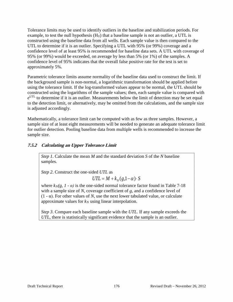
Tolerance limits may be used to identify outliers in the baseline and stabilization periods. For example, to test the null hypothesis (H0) that a baseline sample is not an outlier, a UTL is constructed using the baseline data from all wells. Each sample value is then compared to the UTL to determine if it is an outlier. Specifying a UTL with 95% (or 99%) coverage and a confidence level of at least 95% is recommended for baseline data sets. A UTL with coverage of 95% (or 99%) would be exceeded, on average by less than 5% (or 1%) of the samples. A confidence level of 95% indicates that the overall false positive rate for the test is set to approximately 5%.
Parametric tolerance limits assume normality of the baseline data used to construct the limit. If the background sample is non-normal, a logarithmic transformation should be applied before using the tolerance limit. If the log-transformed values appear to be normal, the UTL should be constructed using the logarithms of the sample values; then, each sample value is compared with eUTL to determine if it is an outlier. Measurements below the limit of detection may be set equal to the detection limit, or alternatively, may be omitted from the calculations, and the sample size is adjusted accordingly. Mathematically, a tolerance limit can be computed with as few as three samples. However, a sample size of at least eight measurements will be needed to generate an adequate tolerance limit for outlier detection. Pooling baseline data from multiple wells is recommended to increase the sample size.
7.5.2 Calculating an Upper Tolerance Limit
Step 1. Calculate the mean M and the standard deviation S of the N baseline samples. Step 2. Construct the one-sided UTL as
UTL = M + kN (g,1−α ) ⋅ S where kN(g, 1 - α) is the one-sided normal tolerance factor found in Table 7-18 with a sample size of N, coverage coefficient of g, and a confidence level of (1 - α). For other values of N, use the next lower tabulated value, or calculate approximate values for kN using linear interpolation. Step 3. Compare each baseline sample with the UTL. If any sample exceeds the UTL, there is statistically significant evidence that the sample is an outlier.
Draft Technical Report 176 Revised Draft – November 26, 2012

Table 7-18. One-Sided Upper Tolerance Limit Factors with g% Coverage for Selected Values of N
95% Confidence 99% Confidence N g=90% 95% 99% g=90% 95% 99%
4 4.162 5.144 7.042 7.380 9.083 12.387 5 3.407 4.203 5.741 5.362 6.578 8.939 6 3.006 3.708 5.062 4.411 5.406 7.335 7 2.755 3.399 4.642 3.859 4.728 6.412 8 2.582 3.187 4.354 3.497 4.285 5.812 9 2.454 3.031 4.143 3.240 3.972 5.389
10 2.355 2.911 3.981 3.048 3.738 5.074 11 2.275 2.815 3.852 2.898 3.556 4.829 12 2.210 2.736 3.747 2.777 3.410 4.633 13 2.155 2.671 3.659 2.677 3.290 4.472 14 2.109 2.614 3.585 2.593 3.189 4.337 15 2.068 2.566 3.520 2.521 3.102 4.222 16 2.033 2.524 3.464 2.459 3.028 4.123 17 2.002 2.486 3.414 2.405 2.963 4.037 18 1.974 2.453 3.370 2.357 2.905 3.960 19 1.949 2.423 3.331 2.314 2.854 3.892 20 1.926 2.396 3.295 2.276 2.808 3.832 21 1.905 2.371 3.263 2.241 2.766 3.777 22 1.886 2.349 3.233 2.209 2.729 3.727 23 1.869 2.328 3.206 2.180 2.694 3.681 24 1.853 2.309 3.181 2.154 2.662 3.640 25 1.838 2.292 3.158 2.129 2.633 3.601 26 1.824 2.275 3.136 2.106 2.606 3.566 27 1.811 2.260 3.116 2.085 2.581 3.533 28 1.799 2.246 3.098 2.065 2.558 3.502 29 1.788 2.232 3.080 2.047 2.536 3.473 30 1.777 2.220 3.064 2.030 2.515 3.447 35 1.732 2.167 2.995 1.957 2.430 3.334 40 1.697 2.125 2.941 1.902 2.364 3.249 45 1.669 2.092 2.898 1.857 2.312 3.180 50 1.646 2.065 2.862 1.821 2.269 3.125 55 1.626 2.042 2.833 1.790 2.233 3.078 60 1.609 2.022 2.807 1.764 2.202 3.038 65 1.594 2.005 2.785 1.741 2.176 3.004 70 1.581 1.990 2.765 1.722 2.153 2.974 75 1.570 1.976 2.748 1.704 2.132 2.947 80 1.559 1.964 2.733 1.688 2.114 2.924 85 1.550 1.954 2.719 1.674 2.097 2.902 90 1.542 1.944 2.706 1.661 2.082 2.883 95 1.534 1.935 2.695 1.650 2.069 2.866
100 1.527 1.927 2.684 1.639 2.056 2.850 Source: Odeh and Owen (1980)
Draft Technical Report 177 Revised Draft – November 26, 2012
7.6 Determining the Number of Samples per Well
The procedure for calculating the number of post-restoration samples for determining compliance must address three kinds of comparisons with baseline conditions:
(1) Comparison of post-restoration samples from an individual monitoring well with the baseline samples from that well
(2) Comparison of post-restoration samples from an individual monitoring well with the pooled samples from all baseline wells
(3) Comparison of pooled post-restoration samples from all monitoring wells with the pooled samples all baseline wells
The number of samples may be determined using several approaches. The first, and most basic, approach is based on the assumptions that the number of samples collected post-restoration is the same as the number of samples collected in the baseline period, and that the standard deviations are the same. Let m and σ1 denote the baseline sample size and standard deviation, and n and σ2 denote the post-restoration sample size and standard deviation. The first approach is based on the assumptions that the sample size is the same in both periods (n=m) and that the standard deviations are the same (σ2=σ1). These constraints preclude most practical applications in comparisons with different sample sizes in the baseline and post-restoration periods. For each of the three kinds of comparisons, the sample size and standard deviation will be the same only in unusual cases.
Generalizing to an approach which permits different sample sizes offers greater flexibility than is available in the first approach, but at a cost. The cost is additional complexity in the form of a larger number of tables for determining sample size. This is necessary in order to span the possible ranges of baseline versus post-restoration sample sizes, as well as several combinations of the DQO parameters α and β, and a range of possible values for the resolution of the test MDD/σ1.
Further generalization to a third approach which permits both different sample sizes and different standard deviations offers additional flexibility than is available in the second approach, but with additional complexity. This is necessary in order to span the possible ranges of baseline versus post-operational sample variability, in addition to the parameters noted for the second approach.
Power and sample size calculations tend to be much more difficult for nonparametric procedures than for parametric procedures. Nonparametric procedures usually have less statistical power than parametric tests when the data follow a known distribution. An adjustment factor of 1.16 is usually applied to account for the possible loss of efficiency when the nonparametric WRS test is
Draft Technical Report 178 Revised Draft – November 26, 2012
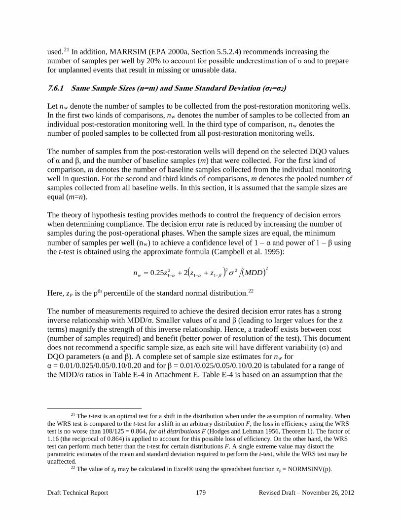
used.21 In addition, MARRSIM (EPA 2000a, Section 5.5.2.4) recommends increasing the number of samples per well by 20% to account for possible underestimation of σ and to prepare for unplanned events that result in missing or unusable data.
7.6.1 Same Sample Sizes (n=m) and Same Standard Deviation (σ1=σ2)
Let nw denote the number of samples to be collected from the post-restoration monitoring wells. In the first two kinds of comparisons, nw denotes the number of samples to be collected from an individual post-restoration monitoring well. In the third type of comparison, nw denotes the number of pooled samples to be collected from all post-restoration monitoring wells. The number of samples from the post-restoration wells will depend on the selected DQO values of α and β, and the number of baseline samples (m) that were collected. For the first kind of comparison, m denotes the number of baseline samples collected from the individual monitoring well in question. For the second and third kinds of comparisons, m denotes the pooled number of samples collected from all baseline wells. In this section, it is assumed that the sample sizes are equal (m=n). The theory of hypothesis testing provides methods to control the frequency of decision errors when determining compliance. The decision error rate is reduced by increasing the number of samples during the post-operational phases. When the sample sizes are equal, the minimum number of samples per well (nw) to achieve a confidence level of 1 − α and power of 1 − β using the t-test is obtained using the approximate formula (Campbell et al. 1995):
( ) ( )2211
21 225.0 MDDzzznw σβαα −−− ++=
2
Here, zp is the pth percentile of the standard normal distribution.22 The number of measurements required to achieve the desired decision error rates has a strong inverse relationship with MDD/σ. Smaller values of α and β (leading to larger values for the z terms) magnify the strength of this inverse relationship. Hence, a tradeoff exists between cost (number of samples required) and benefit (better power of resolution of the test). This document does not recommend a specific sample size, as each site will have different variability (σ) and DQO parameters (α and β). A complete set of sample size estimates for nw for α = 0.01/0.025/0.05/0.10/0.20 and for β = 0.01/0.025/0.05/0.10/0.20 is tabulated for a range of the MDD/σ ratios in Table E-4 in Attachment E. Table E-4 is based on an assumption that the
21 The t-test is an optimal test for a shift in the distribution when under the assumption of normality. When he WRS test is compared to the t-test for a shift in an arbitrary distribution F, the loss in efficiency using the WRS est is no worse than 108/125 = 0.864, for all distributions F (Hodges and Lehman 1956, Theorem 1). The factor of .16 (the reciprocal of 0.864) is applied to account for this possible loss of efficiency. On the other hand, the WRS est can perform much better than the t-test for certain distributions F. A single extreme value may distort the arametric estimates of the mean and standard deviation required to perform the t-test, while the WRS test may be naffected.
22 The value of zp may be calculated in Excel® using the spreadsheet function zp = NORMSINV(p).
tt1tpu
Draft Technical Report 179 Revised Draft – November 26, 2012

sample size for the baseline is the same as the sample size for the post-restoration period (m=n) and that the standard deviations are the same (σ2=σ1).
7.6.2 Different Sample Sizes (n≠m), Same Standard Deviations (σ1=σ2)
The formula for the number of samples when the sample sizes are unequal is provided by Campbell et al. (1995). This formula uses the number of samples when the sample sizes are equal (nw = m = n) given in Section 7.6.1 as the starting point for determining unequal sample sizes. When m is known in advance and is larger than nw/2, the number of samples per well in the post-restoration period is given by:
w
ww nm
n−
=′2
mn
When the number of baseline samples m is smaller than nw/2, there is no value of n that will achieve the DQO parameters α, β, and MDD/σ1 used to calculate the value of nw. When the number of samples in the baseline data set is larger than nw, the number of samples required in the post-restoration period will be smaller than nw, and vice versa. The total number of samples (n+m) will be greater than 2nw when the sample sizes are unequal. This occurs because the use of equal sample sizes is the optimal allocation for achieving the DQO parameters with a minimum number of samples. The values of nw′ are provided for 9 alternative values for α and β in Tables E-5 through E-13. The combinations of the DQO parameters α and β are provided for (α, β) =
(0.05, 0.05), (0.05, 0.10), (0.05, 0.20); (0.10, 0.05), (0.10, 0.10), (0.10, 0.20), (0.20, 0.05), (0.20, 0.10), (0.20, 0.20);
The rows of these tables show the number of samples that were collected in the baseline (m). For the indicated value of m, the columns of the table are indexed by the desired level of resolution MDD/σ.
7.6.3 Different Sample Sizes (n≠m) and Different Standard Deviations (σ1≠σ2)
Generalizing to a model which permits different sample sizes offers greater flexibility than is available in the approach underlying Table E-4, but at a cost. The cost is additional complexity in the form of a larger number of tables for determining sample size. This is necessary to span the wide possible ranges of baseline versus post-restoration sample sizes, baseline versus post-operational sample variability, as well as several combinations of the DQO parameters α and β and the test resolution of MDD/σ1. If there are m baseline samples with standard deviation σ1, the desired degree of resolution for the test is MDD/σ1, and the post-restoration samples are estimated to have standard deviation σ2, then the number of samples nw is the smallest value of n satisfying the inequality:
Draft Technical Report 180 Revised Draft – November 26, 2012
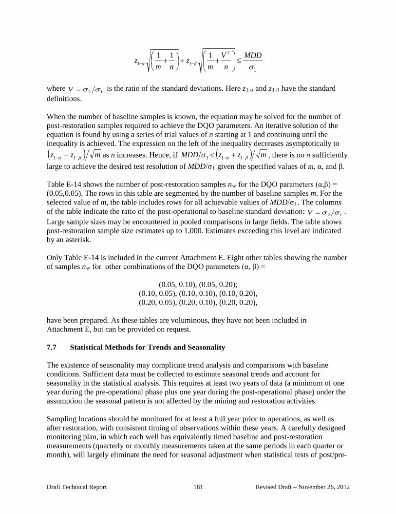
1
2
11111
σβαMDD
nV
mz
nmz ≤
++
+ −−
where V = σ 2 σ1 is the ratio of the standard deviations. Here z1-α and z1-β have the standard definitions. When the number of baseline samples is known, the equation may be solved for the number of post-restoration samples required to achieve the DQO parameters. An iterative solution of the equation is found by using a series of trial values of n starting at 1 and continuing until the inequality is achieved. The expression on the left of the inequality decreases asymptotically to (z1−α + z1−β ) m as n increases. Hence, if MDD σ1 < (z1−α + z1−β ) m , there is no n sufficiently large to achieve the desired test resolution of MDD/σ1 given the specified values of m, α, and β. Table E-14 shows the number of post-restoration samples nw for the DQO parameters (α,β) = (0.05,0.05). The rows in this table are segmented by the number of baseline samples m. For the selected value of m, the table includes rows for all achievable values of MDD/σ1. The columns of the table indicate the ratio of the post-operational to baseline standard deviation: V = σ 2 σ1 . Large sample sizes may be encountered in pooled comparisons in large fields. The table shows post-restoration sample size estimates up to 1,000. Estimates exceeding this level are indicated by an asterisk. Only Table E-14 is included in the current Attachment E. Eight other tables showing the number of samples nw for other combinations of the DQO parameters (α, β) =
(0.05, 0.10), (0.05, 0.20); (0.10, 0.05), (0.10, 0.10), (0.10, 0.20), (0.20, 0.05), (0.20, 0.10), (0.20, 0.20),
have been prepared. As these tables are voluminous, they have not been included in Attachment E, but can be provided on request. 7.7 Statistical Methods for Trends and Seasonality The existence of seasonality may complicate trend analysis and comparisons with baseline conditions. Sufficient data must be collected to estimate seasonal trends and account for seasonality in the statistical analysis. This requires at least two years of data (a minimum of one year during the pre-operational phase plus one year during the post-operational phase) under the assumption the seasonal pattern is not affected by the mining and restoration activities. Sampling locations should be monitored for at least a full year prior to operations, as well as after restoration, with consistent timing of observations within these years. A carefully designed monitoring plan, in which each well has equivalently timed baseline and post-restoration measurements (quarterly or monthly measurements taken at the same periods in each quarter or month), will largely eliminate the need for seasonal adjustment when statistical tests of post/pre-
Draft Technical Report 181 Revised Draft – November 26, 2012

operational differences are performed. Use of consistent timing in both periods has the effect of “subtracting out” any seasonal component when post-restoration data are compared to the initial conditions.
If seasonal patterns are either predicted by hydrological models or observed to be highly variable from year to year, then a single year of pre-operational information may not be adequate. A design in which pre-operational data are collected for more than 1 year may be preferable for ISR operations within shallow aquifers. This is especially true in unusual years of extreme drought or flooding, for example, that may bias the baseline measurements one way or another. One approach for extending the time seasonality is monitored is the use of additional monitoring data collected outside the ore zone. Up gradient wells may be monitored for seasonal effects throughout operational period in lieu of additional pre-operational monitoring.
The first step in analyzing measurements in one or more wells is to plot the data as a time series. Such plots are shown in the example discussed in Attachment D. Plots of the data may reveal patterns such as seasonality and/or the existence of outliers or blunders in the data. Outliers are values that appear to be unusually high or low when compared to the other values. Outliers may be valid data or may arise from unusual circumstances unrelated to the process being measured. Blunders are outright errors made in recording the data, transcription, or calculations. A common blunder is a mistake in the units of measure. Plotting is used to detect these situations, but does not provide for an explanation or resolution for the unusual value. Blunders are sometimes outliers and thus a given value could be both. But blunders need not be outliers—data may have been keyed in wrong but not be far from the main body of observations. So plotting will not always reveal blunders in the data.
If a value is identified as erroneous, it should be removed from the data set. In cases of doubt, the value should be retained. The nonparametric statistical tests discussed in this section were selected because of their robustness. The statistical term “robust” is loosely defined as resistant to the effects of outliers and blunders in the data.
7.7.1 Adjusting for Seasonality
Seasonality may occur in baseline samples in Phase 1, while the site is reaching steady state in Phase 4 and/or in Phase 5, where seasonality may affect decisions concerning long-term stability and whether target remediation values are attained.
Seasonality is a pattern that repeats periodically in a cycle. An annual seasonal pattern has a cycle that spans 12 months or 4 quarters. A seasonal index measures how far the average for a particular period is above (or below) the average for all periods. The unified guidance for RCRA (EPA 2009) recommends the following concerning seasonality:
Seasonal fluctuations in intrawell background can be treated in one of two ways. A seasonal Mann-Kendall trend test built to accommodate such fluctuations can be employed (Section 14.3.4). Otherwise, the seasonal pattern can be estimated and removed from the background data, leaving a set of seasonally-adjusted data to be analyzed with either a prediction limit or control chart. In this latter approach, the same seasonal pattern needs to be extrapolated beyond the current
Draft Technical Report 182 Revised Draft – November 26, 2012

background to more recent measurements from the compliance well being tested. These later observations also need to be seasonally-adjusted prior to comparison against the adjusted background, even if there is not enough compliance data yet collected to observe the same seasonal cycles.
However, the guidance adds the following caveat:
Corrections for seasonality should be used cautiously, as they represent extrapolation into the future. There should be a good physical explanation for the seasonal fluctuation as well as good empirical evidence for seasonality before corrections are made. Higher than average rainfall for two or three Augusts in a row does not justify the belief that there will never be a drought in August, and this idea extends directly to groundwater quality. At least three complete cycles of the seasonal pattern should be observed on a time series plot before attempting the adjustment below. If seasonality is suspected but the pattern is complicated, the user should seek the help of a professional statistician.
The seasonal Mann-Kendall test is a variation of the Mann-Kendall test for trends described below in Section 7.7.2.1. The test is described in detail in EPA 2009 in Section 14.3.4.
Seasonal adjustment procedures are commonly applied to ecological and economic data to account for seasonal patterns. The process of “deseasonalizing” the data removes these periodic seasonal variations to reveal the underlying longer term pattern. The ith seasonal component (Qi) is defined as the deviation of the seasonal mean (Yi) from the overall mean (YM): Qi = Yi - YM. The deseasonalized time series (X) is obtained by subtracting the seasonal means from the original data series: Xt,i = Yt,i - Qi (EPA 2009, Eq. 14.23). The deseasonalized data series has the short-term seasonal variations removed; longer-term trends remain in the data. Plots of the seasonally adjusted data series are useful for determining when suspected outliers in sample values reflect the normal variability of monitored parameters after adjusting for the seasonal variations.
When there are four quarterly measurements in each year, the data may be seasonally adjusted by the procedure described in Section D.1 in Attachment D. Appropriate modifications must be made for periodic variations based on other time frames. Some parameters may require seasonal adjustment and others not. Formal tests for the presence of seasonality across several wells are based on an analysis of variance. This procedure is described in EPA 2002b (Sections 14.2.2 and 14.3.3).
The seasonal adjustment procedures are applicable to data that are approximately symmetric and normally distributed. For highly skewed lognormal data series, the calculations above would be applied to the logarithms of the measurements. This is equivalent to using the ratio of the quarterly mean to the overall mean (Q*
i=Yi/YM) as the seasonality index in place of the additive index above. If this index is 1.2, this means that, on average, the period (season) is 20% higher than average. In this case, the seasonally adjusted data series is obtained by dividing the original data series by the seasonal index: Xt,I = Yt,i/Q*
i.
Draft Technical Report 183 Revised Draft – November 26, 2012

It is assumed that there is a complete set of quarterly measurements for 3 years with no missing or nondetect values. If one or two nondetects occur in the data series, one should replace those values with the limit of detection. If there is at most one missing data value, these methods may be applied using the averages of the available data to compute the seasonal index. If more than one value is missing, the appropriateness of adjusting for seasonal variation should be discussed with a statistician familiar with environmental sampling.
Unless otherwise noted, in the remaining sections of this chapter, the term “data” refers to the seasonally adjusted data series Xt,i.
7.7.2 Using Trend Tests to Determine Stability
Mining by ISR causes a major perturbation of the physical and chemical environment of the ore zone. When mining operations end and restoration activities are completed, the ground water and the minerals it contacts begin to shift toward a new geochemical steady state. It should be recognized that the system may never return to steady-state conditions exactly comparable to pre-operational baseline conditions.
In the short run, post-restoration samples are used to provide statistical evidence of trends or lack thereof. However, the long-term stability of the site is best understood using a conceptual model that considers these data along with the hydrology, contaminant transport, and geochemical reactions to provide a qualitative estimate of the evolution of the system after post-restoration monitoring is completed. The NRC (2007) has emphasized that development of a justifiable conceptual model capturing the major chemical and physical phenomena at each site is required. This approach allows for site-specific flexibility.
In addition to water quality data, mineralogical data can be used to evaluate the long-term stability of the system. Hydro-geochemical modeling can be a valuable tool for modeling the rate of the return to stability and for predicting how long a system will take to return to baseline conditions. Although complete mineralogical characterization may require additional resources, a fully developed quantitative model supported by site post-restoration measurements can provide additional confidence that the restoration goal of site stability after closure has been met.
Statistical tests for trends are used to demonstrate stability within the specified monitoring period. These tests may be used with any time series of four or more independent samples to test for trends in well parameters. Trend tests are employed in Phase 1 to check for unexpected trends in baseline samples, and particularly in Phase 5 to affirm long-term stability. Trends may be detected using parametric and/or nonparametric statistical tests. The power of a trend test to detect a trend depends on several factors, including the underlying variability of the series, the magnitude of slope we wish to detect, level of confidence for the test and the length of time the series is observed.
Draft Technical Report 184 Revised Draft – November 26, 2012

A Monte Carlo simulation was conducted to examine the time it takes to detect a trend. Two popular methods of trend detection are considered: the linear regression t-test23 and the Mann-Kendall test. The regression t-test is a parametric statistical test, and the Mann-Kendall test is a nonparametric test.
7.7.2.1 Detecting Trends Using Hypothesis Tests
Given a series of T sample values x1,, xT collected from a well at times t1,, tT , the objective is to decide if there is a significant trend in the series. In general, time may be measured in any units, such as months, quarters, or years. However, the interpretation of the slope of the trend line will depend on the units selected for the time axis as well as the units of measurement for the sample values. In this discussion, quarterly sampling is assumed as quarterly measurements are commonly used. Sampling frequencies other than quarterly sampling are discussed in Section 7.7.2.4. The time variable is measured in number of years from the first observation. The slope estimates are expressed as a percentage change per year. The simulations assume that the sample collection times are equally spaced, one per quarter. In general, this is not a necessary assumption. Both methods of trend detection may be applied with irregularly spaced sampling times. The linear trend model provides a parametric statistical test for a significant trend in the percentage deviations. A linear trend is described by a trend line with the equation:
Tjbtay jj ,,1, =+=
Here the coefficient a is the initial value of y at time t=0, often described as the intercept of the trend line. The coefficient b is the slope of the trend line. If time is increased by one unit, the value of y is increased (or decreased) by b units when b is positive (or negative). The regression t-test is used to test if an observed positive or negative slope in the series is statistically significant at a specified level of confidence. The t-statistic for the test is the slope estimate b̂ divided by its standard error of estimation: t(b̂) = b̂ SE(b̂) . If the absolute value of thet-statistic for the slope coefficient is larger than the critical value for the test, then the trend has a significantly positive (or negative) slope. If the slope of the trend line is not zero, all statistical tests will detect the trend eventually. In the short term, the test may or may not detect a trend. The power to detect a trend will depend on the magnitude of the trend, the degree of temporal variability, the level of confidence for the test, and how long we are willing to wait to detect the trend. A complete discussion of the use of linear and nonlinear regression models for assessing trends is provided in Chapter 6 of EPA 1992.
7.7.2.2 Simulation of Trend Detection
23 A complete discussion of linear regression techniques for assessing trends and projecting probable future evels is found in EPA 1992, Chapter 6. l
Draft Technical Report 185 Revised Draft – November 26, 2012
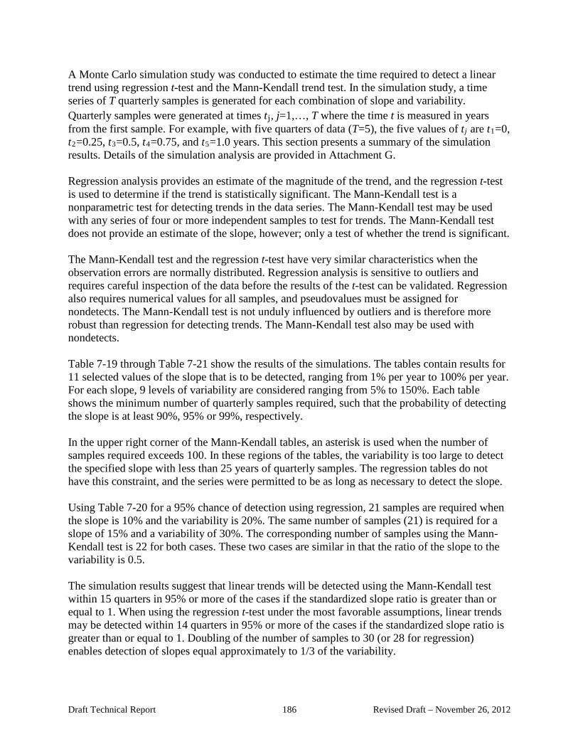
A Monte Carlo simulation study was conducted to estimate the time required to detect a linear trend using regression t-test and the Mann-Kendall trend test. In the simulation study, a time series of T quarterly samples is generated for each combination of slope and variability. Quarterly samples were generated at times tj, j=1,…, T where the time t is measured in years from the first sample. For example, with five quarters of data (T=5), the five values of tj are t1=0, t2=0.25, t3=0.5, t4=0.75, and t5=1.0 years. This section presents a summary of the simulation results. Details of the simulation analysis are provided in Attachment G.
Regression analysis provides an estimate of the magnitude of the trend, and the regression t-test is used to determine if the trend is statistically significant. The Mann-Kendall test is a nonparametric test for detecting trends in the data series. The Mann-Kendall test may be used with any series of four or more independent samples to test for trends. The Mann-Kendall test does not provide an estimate of the slope, however; only a test of whether the trend is significant.
The Mann-Kendall test and the regression t-test have very similar characteristics when the observation errors are normally distributed. Regression analysis is sensitive to outliers and requires careful inspection of the data before the results of the t-test can be validated. Regression also requires numerical values for all samples, and pseudovalues must be assigned for nondetects. The Mann-Kendall test is not unduly influenced by outliers and is therefore more robust than regression for detecting trends. The Mann-Kendall test also may be used with nondetects.
Table 7-19 through Table 7-21 show the results of the simulations. The tables contain results for 11 selected values of the slope that is to be detected, ranging from 1% per year to 100% per year. For each slope, 9 levels of variability are considered ranging from 5% to 150%. Each table shows the minimum number of quarterly samples required, such that the probability of detecting the slope is at least 90%, 95% or 99%, respectively.
In the upper right corner of the Mann-Kendall tables, an asterisk is used when the number of samples required exceeds 100. In these regions of the tables, the variability is too large to detect the specified slope with less than 25 years of quarterly samples. The regression tables do not have this constraint, and the series were permitted to be as long as necessary to detect the slope.
Using Table 7-20 for a 95% chance of detection using regression, 21 samples are required when the slope is 10% and the variability is 20%. The same number of samples (21) is required for a slope of 15% and a variability of 30%. The corresponding number of samples using the Mann-Kendall test is 22 for both cases. These two cases are similar in that the ratio of the slope to the variability is 0.5.
The simulation results suggest that linear trends will be detected using the Mann-Kendall test within 15 quarters in 95% or more of the cases if the standardized slope ratio is greater than or equal to 1. When using the regression t-test under the most favorable assumptions, linear trends may be detected within 14 quarters in 95% or more of the cases if the standardized slope ratio is greater than or equal to 1. Doubling of the number of samples to 30 (or 28 for regression) enables detection of slopes equal approximately to 1/3 of the variability.
Draft Technical Report 186 Revised Draft – November 26, 2012

Table 7-19. Number of Quarterly Samples Required for 90% Probability of Detecting Slope Using a Mann-Kendall or Regression Trend Test
Regression Trend Test Mann-Kendall Trend Test
Variability (%) Variability (%) Slope Slope (%/year) (%/year) 5 10 15 20 30 50 75 100 150 5 10 15 20 30 50 75 100 150
1 36 56 73 88 114 161 210 254 333 1 37 57 74 90 * * * * * 3 18 27 35 43 56 78 101 122 159 3 18 28 37 44 57 78 * * * 5 13 20 26 31 40 56 72 87 114 5 13 20 26 32 41 57 75 89 *
10 9 13 17 20 26 36 46 56 73 10 9 13 17 20 27 36 47 57 74 15 7 10 13 15 20 27 35 43 56 15 8 11 13 16 21 28 36 44 57 20 6 9 11 13 16 23 30 35 46 20 7 9 12 13 17 24 30 37 47 30 5 7 9 10 13 18 23 27 35 30 6 8 9 11 14 18 24 28 37 40 5 6 7 9 11 15 19 23 30 40 5 7 8 9 11 15 20 24 31 50 4 6 7 8 10 13 16 20 26 50 5 6 7 9 10 13 17 20 27 75 4 5 5 6 8 10 13 15 20 75 4 5 6 7 9 11 13 16 20
100 4 * Over 100 quarters.
4 Mann
5 -Ken
5 dall te
7 st sim
9 ulation
11 is limi
13 ted to 2
17 100 4 5 years.
5 5 6 7 9 12 13 17
Draft Technical Report 187 Revised Draft – November 26, 2012

Table 7-20. Number of Quarterly Samples Required for 95% Probability of Detecting Slope Using a Mann-Kendall or Regression Trend Test
Regression Trend Test Mann-Kendall Trend Test
Slope Variability (%) Variability (%) Slope (%/year) (%/year) 5 10 15 20 30 50 75 100 150 5 10 15 20 30 50 75 100 150
1 38 61 79 95 124 175 225 271 358 1 39 62 80 97 * * * * * 3 19 30 38 46 60 84 109 133 175 3 20 30 39 47 62 85 * * * 5 14 21 27 33 44 60 79 96 123 5 14 22 29 34 44 62 80 97 *
10 9 14 18 21 28 39 50 60 79 10 10 14 18 22 29 40 51 62 80 15 7 11 14 17 21 30 38 46 60 15 8 12 14 17 22 31 39 47 61 20 6 9 12 14 18 25 32 39 50 20 7 10 12 14 19 25 32 39 52 30 5 7 9 11 14 19 24 30 38 30 6 8 10 12 15 20 25 31 39 40 5 6 8 9 11 16 20 25 32 40 5 7 9 10 12 16 21 25 33 50 5 6 7 8 10 14 18 21 27 50 5 7 8 9 11 14 18 22 28 75 4 5 6 7 8 11 14 17 21 75 4 5 7 7 9 12 14 17 22
100 4 * Over 100 quarters.
4 Mann
5 -Ken
6 dall te
7 st sim
9 ulation
12 is limi
14 ted to 2
18 100 4 5 years.
5 6 7 8 10 12 14 18
Draft Technical Report 188 Revised Draft – November 26, 2012

Table 7-21. Number of Quarterly Samples Required for 99% Probability of Detecting Slope Using a Mann-Kendall or Regression Trend Test
Regression Trend Test Mann-Kendall Trend Test Slope Variability (%) Variability (%) Slope (%/year) (%/year) 5 10 15 20 30 50 75 100 150 5 10 15 20 30 50 75 100 150
1 43 68 89 106 139 197 258 306 405 1 45 70 91 * * * * * * 3 21 34 44 52 68 95 123 150 198 3 22 34 44 54 70 96 * * * 5 16 24 31 37 49 68 88 108 136 5 16 25 32 39 50 70 90 * *
10 10 15 20 24 32 43 56 69 89 10 11 16 21 25 32 45 58 69 89 15 8 12 15 19 24 33 43 52 68 15 9 13 16 20 25 34 45 53 69 20 7 10 13 15 20 28 36 43 56 20 8 11 14 16 21 29 37 44 58 30 6 8 10 12 15 21 28 33 43 30 7 9 11 13 16 22 29 34 45 40 5 7 9 10 13 18 23 28 36 40 6 8 10 11 14 18 24 28 38 50 5 6 8 9 11 16 20 24 31 50 5 7 9 10 12 16 21 25 32 75 4 5 6 7 9 12 15 19 24 75 5 6 7 8 10 13 16 19 25
100 4 * Over 100 quarters.
5 Mann
6 -Ken
6 dall te
8 st simu
10 lation
13 is limi
16 ted to 2
20 100 4 5 years.
5 7 7 9 11 14 16 20
Draft Technical Report 189 Revised Draft – November 26, 2012

7.7.2.3 Duration of Sampling
Table 7-20 shows the required number of samples to achieve a 95% probability of detection using the regression t-test or the Mann-Kendall test for selected slope and variability. The simulation results also provide estimates of the probability of detecting a trend using a fixed number of quarterly samples. This section presents a comparison of three alternatives: quarterly sampling for 12 quarters (3 years); 20 quarters (5 years); or 32 quarters (8 years). The comparison uses the same set of slopes and variability as in Table 7-20.
Table 7-22 shows the probability of detecting a trend (expressed as a percentage) using the Mann-Kendall trend test or the regression t-test with 12 quarterly samples. The probability of detection was simulated for the combinations of slope and variability shown on the borders of the tables. The slope is expressed as the percentage change per year, and the variability is expressed in terms of the standard deviation from the trend line. The outlined cells on the diagonal of the table indicate where the slope is equal to the variability.
Using 12 quarterly samples, there is approximately an 80% chance of detecting the trend using the Mann-Kendall test when the slope is equal to the variability. When the regression t-test is used with normally distributed observation errors, the chance of detection increases to approximately 87% when the slope is equal to the variability. When the slope is less than the variability, the probability of detection is always smaller than these values, falling quickly to below 50%. The apparently better performance of the regression t-test over the Mann-Kendall test is largely due to the fact that the simulation uses normally distributed errors.
Table 7-23 shows simulation results for 20 quarterly samples spread over 5 years. There is approximately a 100% chance of detecting the trend when the slope is equal to the variability. Table 7-24 shows simulation results for 32 quarterly samples (8 years). In this case, the chance of detecting slopes as small as one-half of the variability is approximately 100%.
Draft Technical Report 190 Revised Draft – November 26, 2012
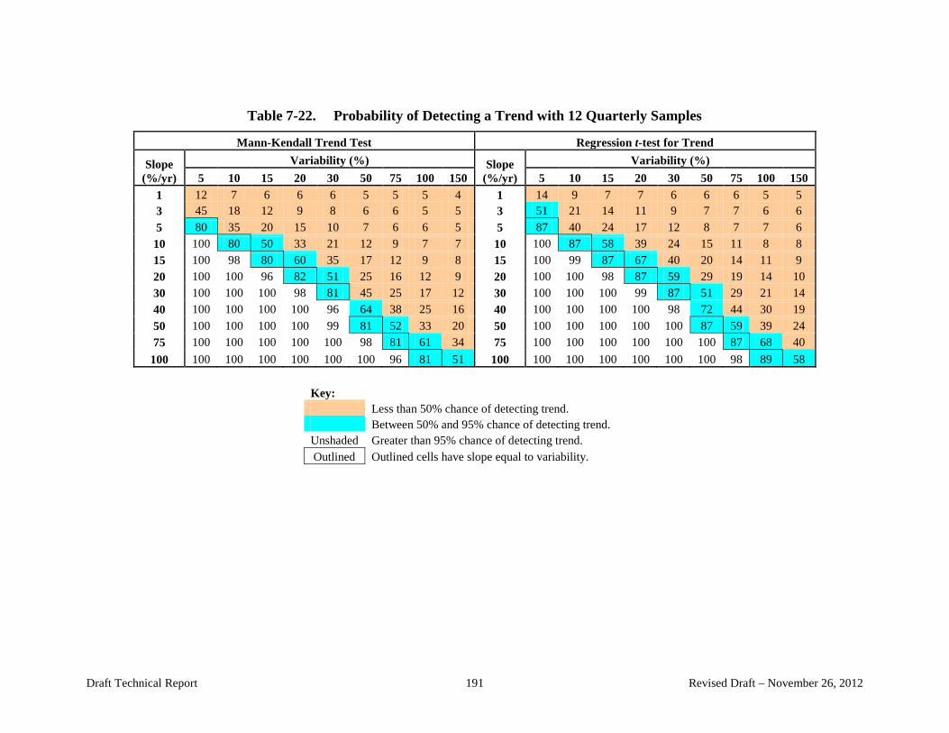
Table 7-22. Probability of Detecting a Trend with 12 Quarterly Samples
Mann-Kendall Trend Test Regression t-test for Trend Variability (%) Variability (%) Slope Slope
(%/yr) 5 10 15 20 30 50 75 100 150 (%/yr) 5 10 15 20 30 50 75 100 150 1 12 7 6 6 6 5 5 5 4 1 14 9 7 7 6 6 6 5 5 3 45 18 12 9 8 6 6 5 5 3 51 21 14 11 9 7 7 6 6 5 80 35 20 15 10 7 6 6 5 5 87 40 24 17 12 8 7 7 6 10 100 80 50 33 21 12 9 7 7 10 100 87 58 39 24 15 11 8 8 15 100 98 80 60 35 17 12 9 8 15 100 99 87 67 40 20 14 11 9 20 100 100 96 82 51 25 16 12 9 20 100 100 98 87 59 29 19 14 10 30 100 100 100 98 81 45 25 17 12 30 100 100 100 99 87 51 29 21 14 40 100 100 100 100 96 64 38 25 16 40 100 100 100 100 98 72 44 30 19 50 100 100 100 100 99 81 52 33 20 50 100 100 100 100 100 87 59 39 24 75 100 100 100 100 100 98 81 61 34 75 100 100 100 100 100 100 87 68 40
100 100 100 100 100 100 100 96 81 51 100 100 100 100 100 100 100 98 89 58
Key: Less than 50% chance of detecting trend. Between 50% and 95% chance of detecting trend.
Unshaded Greater than 95% chance of detecting trend. Outlined Outlined cells have slope equal to variability.
Draft Technical Report 191 Revised Draft – November 26, 2012
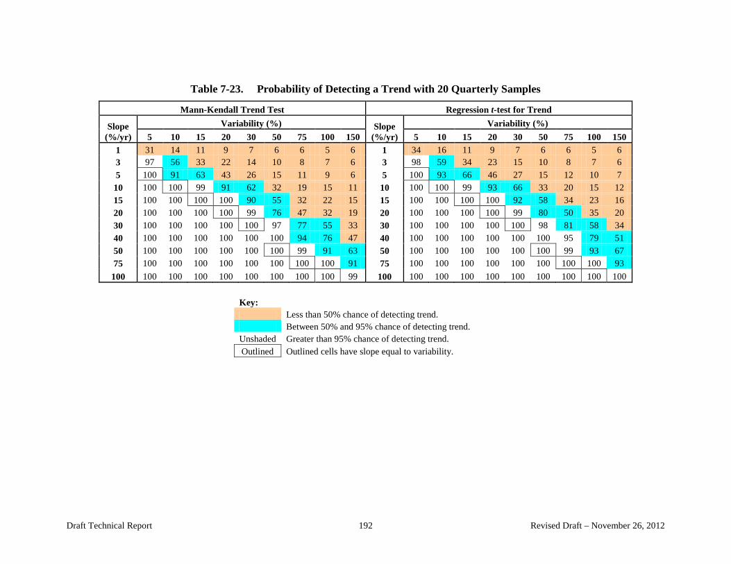
Table 7-23. Probability of Detecting a Trend with 20 Quarterly Samples
Mann-Kendall Trend Test Regression t-test for Trend Variability (%) Variability (%) Slope Slope
(%/yr) 5 10 15 20 30 50 75 100 150 (%/yr) 5 10 15 20 30 50 75 100 150 1 31 14 11 9 7 6 6 5 6 1 34 16 11 9 7 6 6 5 6 3 97 56 33 22 14 10 8 7 6 3 98 59 34 23 15 10 8 7 6 5 100 91 63 43 26 15 11 9 6 5 100 93 66 46 27 15 12 10 7 10 100 100 99 91 62 32 19 15 11 10 100 100 99 93 66 33 20 15 12 15 100 100 100 100 90 55 32 22 15 15 100 100 100 100 92 58 34 23 16 20 100 100 100 100 99 76 47 32 19 20 100 100 100 100 99 80 50 35 20 30 100 100 100 100 100 97 77 55 33 30 100 100 100 100 100 98 81 58 34 40 100 100 100 100 100 100 94 76 47 40 100 100 100 100 100 100 95 79 51 50 100 100 100 100 100 100 99 91 63 50 100 100 100 100 100 100 99 93 67 75 100 100 100 100 100 100 100 100 91 75 100 100 100 100 100 100 100 100 93
100 100 100 100 100 100 100 100 100 99 100 100 100 100 100 100 100 100 100 100
Key: Less than 50% chance of detecting trend. Between 50% and 95% chance of detecting trend.
Unshaded Greater than 95% chance of detecting trend. Outlined Outlined cells have slope equal to variability.
Draft Technical Report 192 Revised Draft – November 26, 2012

Table 7-24. Probability of Detecting a Trend with 32 Quarterly Samples
Mann-Kendall Trend Test Regression t-test for Trend Variability (%) Variability (%) Slope Slope
(%/yr) 5 10 15 20 30 50 75 100 150 (%/yr) 5 10 15 20 30 50 75 100 150 1 78 33 19 14 10 8 7 6 5 1 81 36 21 15 10 9 7 7 6 3 100 98 78 58 33 19 12 10 8 3 100 99 82 61 35 20 13 10 8 5 100 100 99 92 66 33 19 14 9 5 100 100 100 94 70 35 21 16 10 10 100 100 100 100 99 78 49 33 20 10 100 100 100 100 99 81 52 35 22 15 100 100 100 100 100 98 78 58 33 15 100 100 100 100 100 99 81 61 35 20 100 100 100 100 100 100 95 78 48 20 100 100 100 100 100 100 97 82 53 30 100 100 100 100 100 100 100 98 80 30 100 100 100 100 100 100 100 98 83 40 100 100 100 100 100 100 100 100 95 40 100 100 100 100 100 100 100 100 96 50 100 100 100 100 100 100 100 100 99 50 100 100 100 100 100 100 100 100 100 75 100 100 100 100 100 100 100 100 100 75 100 100 100 100 100 100 100 100 100
100 100 100 100 100 100 100 100 100 100 100 100 100 100 100 100 100 100 100 100
Key: Less than 50% chance of detecting trend. Between 50% and 95% chance of detecting trend.
Unshaded Greater than 95% chance of detecting trend. Outlined Outlined cells have slope equal to variability.
Draft Technical Report 193 Revised Draft – November 26, 2012

7.7.2.4 Sampling Frequency
When the sampling frequency changes from the base case of one sample per quarter to a higher or lower frequency (say bi-annual or monthly), there are several important factors to consider. Higher sampling frequencies increase the possibility that there will be correlations between successive samples. The simulation model described above does not consider correlations in the series of samples. If there are possible correlations, the required number of samples is larger than the simulation predicts. In the unlikely case of negative correlations, the required number of samples would be smaller than the simulation predicts. In the following discussion, correlation is ignored.
In the absence of correlation, higher sampling frequencies affect the required number of samples in two opposite ways. A higher sampling frequency provides a greater number of samples, but in a shorter period of time. The effect of a greater number of samples is clear: it will increase the power of detection. However, a shorter period of observation means that the time series does not have as long to change and the change that has occurred is more difficult to detect.
To explore the implications of higher or lower sampling frequencies in the absence of correlation, one case in Table 7-20 was selected for a “one-off” analysis. Table 7-20 was generated using 4 quarterly samples per year. The case in Table 7-20 for a 95% chance of detecting a slope of 10%/year and a variability of 20% was selected for this analysis. This case requires 21 samples for a 95% chance of detection using regression, and 22 samples using the Mann-Kendall test when sampling is conducted quarterly.
Sampling frequencies of 2 per year (semiannual), 4 per year (quarterly), 8 per year (approximately 6-week intervals), and 12 per year (monthly) were selected for the simulation analysis. Table 7-25 shows results of the simulation. The selected case from Table 7-20 is highlighted in this table at a sampling frequency of 4 samples per year.
When the sampling frequency is reduced to semiannual (2 per year), the required number of samples for detecting a trend using the regression t-test is reduced from 21 quarterly samples to 14 semiannual samples. It will take 7 years to collect the 14 semiannual samples, compared with 5.25 years to collect 21 quarterly samples. Results for the regression t-test and the Mann-Kendall test are almost identical. In the absence of correlation, less frequent sampling requires fewer sampling events, but the samples are spread over a longer period of time. It is more unlikely to encounter correlations using semiannual data than using quarterly data, so this result of the one-off analysis is reasonably robust with respect to the assumed lack of correlation.
If sampling is conducted more frequently than quarterly, more samples are required. If a 6-week sampling interval is used (approximately 8 per year), the required number of samples for detecting a trend using regression is increased from 21 quarterly samples to 33 samples. It will take slightly over 4 years to collect the 33 six-week samples, compared with 5.25 years to collect 21 quarterly samples. In the absence of correlation, more frequent sampling requires more sampling events, but the samples are spread over a shorter period of time. If a monthly sampling interval is used (12 per year), the required number of samples for detecting a trend using regression is increased to 43 samples. It will take approximately 3.5 years to collect the 43
Draft Technical Report 194 Revised Draft – November 26, 2012
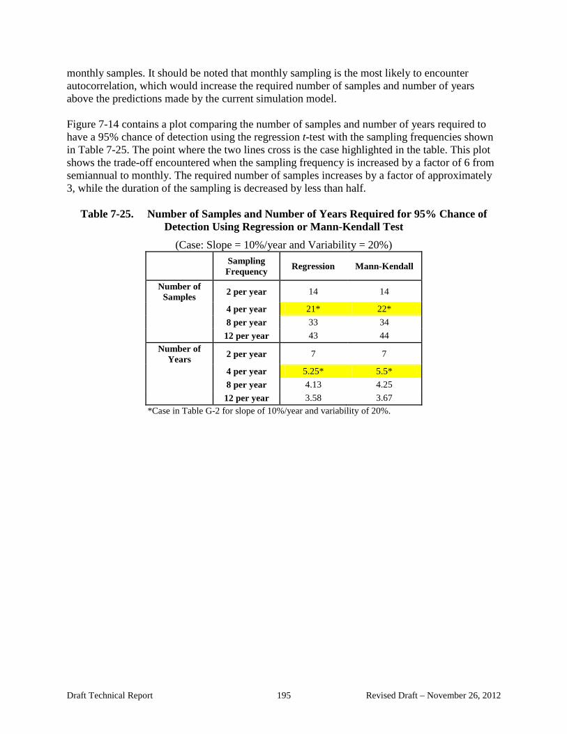
monthly samples. It should be noted that monthly sampling is the most likely to encounter autocorrelation, which would increase the required number of samples and number of years above the predictions made by the current simulation model. Figure 7-14 contains a plot comparing the number of samples and number of years required to have a 95% chance of detection using the regression t-test with the sampling frequencies shown in Table 7-25. The point where the two lines cross is the case highlighted in the table. This plot shows the trade-off encountered when the sampling frequency is increased by a factor of 6 from semiannual to monthly. The required number of samples increases by a factor of approximately 3, while the duration of the sampling is decreased by less than half.
Table 7-25. Number of Samples and Number of Years Required for 95% Chance of Detection Using Regression or Mann-Kendall Test
(Case: Slope = 10%/year and VariabiliSampling Regression Frequency
Number of 2 per year 14 Samples 4 per year 21* 8 per year 33
ty = 20%)
Mann-Kendall
14
22* 34
12 per year 43 Number of 2 per year 7 Years
4 per year 5.25* 8 per year 4.13
44
7
5.5* 4.25
12 per year 3.58 3.67 *Case in Table G-2 for slope of 10%/year and variability of 20%.
Draft Technical Report 195 Revised Draft – November 26, 2012

50
noi 45
ect
et Df 40
ce o
35
anno
h C es
si 30 9
5%r
eg 25
r Ro g f ned si 20
r Uiu 15
eq R
er 10
bmu 5
N
00 1 2 3 4 5 6 7 8 9 10 11 12 13
Sampling Frequency (#/year)
# of Samples # of Quarters
Figure 7-14. Plot of Number of Samples and Number of Quarters Required for 95% Chance of Detection Using Regression versus Sampling Frequency
(Case: Slope = 10%/year and Variability = 20%)
7.7.2.5 Caveats Concerning Regression Analysis of Trends
The linear regression model provides estimates of the slope of the trend line and its standard error based on least squares. The ratio of these estimates is the t-statistic used in the regression t-test for a significant slope. Many parametric tests like the linear regression t-test are based on the normality assumption or equivalent. These tests perform well when the observation errors are normally distributed. When the observation errors are not normally distributed and include random outliers, the least squares estimates of the slope of the regression line and its standard error may be unduly influenced by these outliers. When regression analysis is used, it is important to verify the assumptions, including:
• Normality of residuals • Equal variances • Independence • Sensitivity to outliers
The Mann-Kendall test is a nonparametric test for trends. Both tests have very similar characteristics when the observation errors are normally distributed. This fact is confirmed by the similarity of simulation results for these tests in Table 7-19 through Table 7-24. Unlike the
Draft Technical Report 196 Revised Draft – November 26, 2012
regression -test, the Mann-Kendall test also is expected to perform well when the errors of observation are not normally distributed. The two tests also differ in the treatment of nondetect values. The Mann-Kendall test is based on counts of how many observations are higher, lower, or the same as the ones before. When the time series contains nondetect values, the counts are made by treating all nondetects as equal and assuming all other values in the series are greater than the nondetects. The counts may be made without assuming a specific value for the nondetects. Such is not the case with parametric models. The most elementary parametric estimate is to use the arithmetic average as an estimate of the mean. This simple estimate cannot be calculated without assuming values for the nondetects. Estimation using linear regression and least squares is only possible if specific values are used for the nondetects, usually one-half of the detection level. Despite the advantages of the Mann-Kendall test for detecting trends, the test does not provide an estimate of the magnitude of the slope. Other nonparametric methods are available for estimating the slope, including the Theil-Sen trend line estimator.24 The following text was excerpted from EPA QA/G-9S (EPA 2006a):
4.3.2.1 Estimating a Trend Using the Slope of the Regression Line The classic procedures for assessing linear trends involve regression. Linear regression is a commonly used procedure in which calculations are performed on a data set containing pairs of observations (Xi, Yi), so as to obtain the slope and intercept of a line that best fits the data. For temporal data, the Xi values represent time and the Yi values represent the observations. An estimate of the magnitude of trend can be obtained by performing a regression of the data versus time and using the slope of the regression line as the measure of the strength of the trend. Regression procedures are easy to apply. All statistical software packages and spreadsheet programs will calculate the slope and intercept of the best fitting line, as well as the correlation coefficient r (see Section 2.2.4). However, regression entails several limitations and assumptions. First of all, simple linear regression (the most commonly used method) is designed to detect linear relationships between two variables; other types of regression models are generally needed to detect non-linear relationships such as cyclical or non-monotonic trends. Regression is very sensitive to outliers and presents difficulties in handling data below the detection limit, which are commonly encountered in environmental studies. Hypothesis testing for linear regression also relies on two key assumptions: normally distributed errors, and constant variance. It may be difficult or burdensome to verify these assumptions in practice, so the accuracy of the slope estimate may be suspect. Moreover, the analyst must ensure that time plots of the data show no cyclical pattern; outlier tests show no extreme data
24 The Theil-Sen trend estimator is described in detail in EPA 2009 in Section 17.3.3. The Mann-Kendall test is also described in EPA 2009 in Section 17.3.2.
Draft Technical Report 197 Revised Draft – November 26, 2012
values; and data validation reports indicate that nearly all the measurements were above detection limits. Due to these drawbacks, linear regression is not recommended as a general tool for estimating and detecting trends, although it may be useful as an informal and quick screening tool for identifying strong linear trends. [Emphasis added.]
The nonparametric Mann-Kendall test for trends is recommended in this document for detecting trends. However, the Mann-Kendall test does not provide an estimate of the magnitude of the trend. Once a trend has been detected using the Mann-Kendall test, an estimate of the magnitude of the trend may be required. In this regard, linear regression may be used to estimate the trend, provided that the assumptions required for linear regression are met. Despite the noted drawbacks to using regression for trend analysis, software for regression is readily available and the technique is widely known. Regression also provides traditional confidence intervals and hypothesis tests for evaluating the significance of a trend. Confidence intervals are also useful for comparing trends of different analytes and different wells.
The assumptions concerning outliers and nondetects may preclude the use of linear regression for estimating the magnitude of the trend. If there are outliers and/or nondetects in the data set, a nonparametric method (the Theil-Sen trend line estimator) may be used to estimate the magnitude of the trend.
7.7.2.6 Testing Multiple Wells for Trends
The Mann-Kendall test is useful for analyzing the trend in data from a single well. If the data were collected systematically across the site at approximately the same sampling times, the Mann-Kendall test statistics Sk for all wells may be combined to make an overall summary for the entire set of wells. In this approach, the statistics Sk are used as a summary measure of the trend in each well. There must be consistency in the data series across wells to make a determination of trend that is valid across all wells.
A single statement applicable to trends across all wells is valid if the wells exhibit approximately steady trends in the same direction (upward or downward), with roughly comparable slopes. Formal statistical tests for the comparability of the data series across wells and for a common trend are described in EPA QA/G9S (EPA 2006a) in the text below. Both tests are based on the chi-squared distribution. The two tests are designed to be implemented sequentially, first testing for comparability of slopes, then for a significant common trend across wells.
The hypothesis tests described in EPA 2006a are:
Comparability of stations. H0: Similar dynamics affect all K stations vs. HA: At least two stations exhibit different dynamics.
Testing for overall monotonic trend. H0*: Contaminant levels do not change over time vs. HA*: There is an increasing (or decreasing) trend consistent across all stations.
Draft Technical Report 198 Revised Draft – November 26, 2012
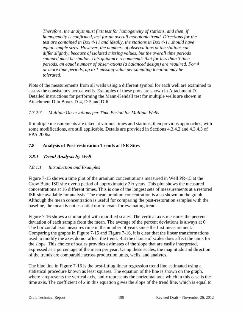
Therefore, the analyst must first test for homogeneity of stations, and then, if homogeneity is confirmed, test for an overall monotonic trend. Directions for the test are contained in Box 4-11 and ideally, the stations in Box 4-11 should have equal sample sizes. However, the numbers of observations at the stations can differ slightly, because of isolated missing values, but the overall time periods spanned must be similar. This guidance recommends that for less than 3 time periods, an equal number of observations (a balanced design) are required. For 4 or more time periods, up to 1 missing value per sampling location may be tolerated.
Plots of the measurements from all wells using a different symbol for each well are examined to assess the consistency across wells. Examples of these plots are shown in Attachment D. Detailed instructions for performing the Mann-Kendall test for multiple wells are shown in Attachment D in Boxes D-4, D-5 and D-6.
7.7.2.7 Multiple Observations per Time Period for Multiple Wells
If multiple measurements are taken at various times and stations, then previous approaches, with some modifications, are still applicable. Details are provided in Sections 4.3.4.2 and 4.3.4.3 of EPA 2006a.
7.8 Analysis of Post-restoration Trends at ISR Sites
7.8.1 Trend Analysis by Well
7.8.1.1 Introduction and Examples
Figure 7-15 shows a time plot of the uranium concentrations measured in Well PR-15 at the Crow Butte ISR site over a period of approximately 3½ years. This plot shows the measured concentrations at 16 different times. This is one of the longest sets of measurements at a restored ISR site available for analysis. The mean uranium concentration is also shown on the graph. Although the mean concentration is useful for comparing the post-restoration samples with the baseline, the mean is not essential nor relevant for evaluating trends. Figure 7-16 shows a similar plot with modified scales. The vertical axis measures the percent deviation of each sample from the mean. The average of the percent deviations is always at 0. The horizontal axis measures time in the number of years since the first measurement. Comparing the graphs in Figure 7-15 and Figure 7-16, it is clear that the linear transformations used to modify the axes do not affect the trend. But the choice of scales does affect the units for the slope. This choice of scales provides estimates of the slope that are easily interpreted, expressed as a percentage of the mean per year. Using these scales, the magnitude and direction of the trends are comparable across production units, wells, and analytes. The blue line in Figure 7-16 is the best-fitting linear regression trend line estimated using a statistical procedure known as least squares. The equation of the line is shown on the graph, where y represents the vertical axis, and x represents the horizontal axis which in this case is the time axis. The coefficient of x in this equation gives the slope of the trend line, which is equal to
Draft Technical Report 199 Revised Draft – November 26, 2012

5.9784 or approximately 6%. On average, the uranium concentration in Well PR-15 is rising at about 6% of the mean per year. Although the symbol x is used to represent the horizontal axis in the figure, the symbol T will be used for the horizontal time axis in the following discussion. The linear trend equation is expressed as yT = α + βT , where yT denotes the percent deviation from the mean value at time T, and T is the number of years from the first measurement. The percent deviation from the mean is calculated as yT = 100 ⋅ (X T − X ) X , where XT denotes the sample concentration at time T and X is the average concentration in the well over the period in question. The symbol β is slope of the line. In Figure 7-16, β = 5.9784% of the mean per year. The symbol α is called the y-intercept, which is the value of the trend line at time T=0. The dashed red lines in Figure 7-16 show the temporal variability of the samples around the trend line. These lines are drawn at plus and minus one standard deviation from the trend line. The positive slope of 6% per year is small relative to the temporal variability of approximately ±60%. The question then arises whether the slope is statistically significant. To test for significance of the slope, it is necessary to compute the standard error of the estimated slope, written as SE(β). Table 7-26 shows the regression results for uranium and radium in well PR-15, the estimates of the slope and intercept, standard errors, R-square, t-statistics and degrees of freedom. The slope estimate β=5.98 is in the upper left corner of the table, and the standard error of the slope estimate SE(β)=10.53 is shown in the row below. The t-statistic used to test for a significant slope is equal to the ratio of the slope to its standard error: tβ = β SE(β ) = 5.98 /10.53 = 0.57 . When the absolute value of the t-statistic is larger than the critical value for the regression t-test, the slope estimate is statistically significant at a specified level of confidence. Usually a 95% level of confidence is required. A table of the critical values for the t-test is provided in Table 7-31. The smallest critical value in the table for 14 degrees of freedom is 1.345 for a 90% confidence level. The t-statistic of uranium is much smaller than the critical value; hence the positive slope observed in Figure 7-16 is not statistically significant. The uranium concentrations are considered stable because there is no significant trend.
Table 7-26. Regression Statistics for Example in Figure 7-16 Uranium (mg/l) Slope Intercept
Estimate-> 5.98 -10.07 Standard Error-> 10.53 22.85
R-square-> 0.02 14 <-Degrees of Freedom
t-statistic-> 0.57 -0.44
Radium (pCi/L) Slope Intercept Estimate-> -10.06 15.27
Standard Error-> 5.24 11.63 R-square-> 0.32
8 <-Degrees of Freedom t-statistic-> -1.92 1.31
Note: An automated tool, such as the linest() function in Excel, can be used to calculate the regression statistics.
Draft Technical Report 200 Revised Draft – November 26, 2012

Figure 7-17 shows the radium concentrations in well PR-15 over the same time period. After a sudden initial rise, the trend is down for the remaining time. The estimated slope is negative 10% per year, indicating that radium concentrations are decreasing in this well. The standard error for the slope in Table 7-26 is 5.24 and the t-statistic is -1.92. In this case, the downward trend is statistically significant at the 95% level of confidence.
One advantage of the Bayesian approach is it allows for straightforward probability comparisons of the slope parameters. Figure 7-18 shows a Bayesian interpretation of the slope estimates obtained using non-informative prior distributions for uranium and radium in well PR-15 at Crow Butte. In this case, a non-informative prior distribution means a prior opinion that all values of the slope are possible, both negative and positive, and of any magnitude. The figure shows the posterior t-distributions for the uranium and radium slope parameters. The uranium posterior t-distribution is very broad, extending well below the 0 value. Although the least squares slope estimate for uranium is positive, the estimated slope is not statistically significant because a large portion of the posterior distribution lies below 0. The radium posterior t-distribution is much narrower, and almost all of the distribution lies below 0. The negative slope estimate for radium is statistically significant.
Figure 7-19 shows the complementary cumulative distribution functions (CCDFs)25 for the posterior distributions in Figure 7-18. These curves show the probability that the slope (expressed as the percent of the mean per year) is greater than the value shown on the horizontal axis. The probability that the trend in radium is greater than 0 is less than 0.05 (5%), while the probability that the trend for uranium is greater than 0 is approximately 0.75 (75%).
Figure 7-20 shows a Bayesian comparison of the trends for radium in wells PR-8 and PR-15 at Crow Butte. Although radium was found to have a significant downward trend in well PR-15, radium has a significant upward trend in well PR-8.
25 The CCDF is defined as one minus the cumulative distribution function (CDF).
Draft Technical Report 201 Revised Draft – November 26, 2012
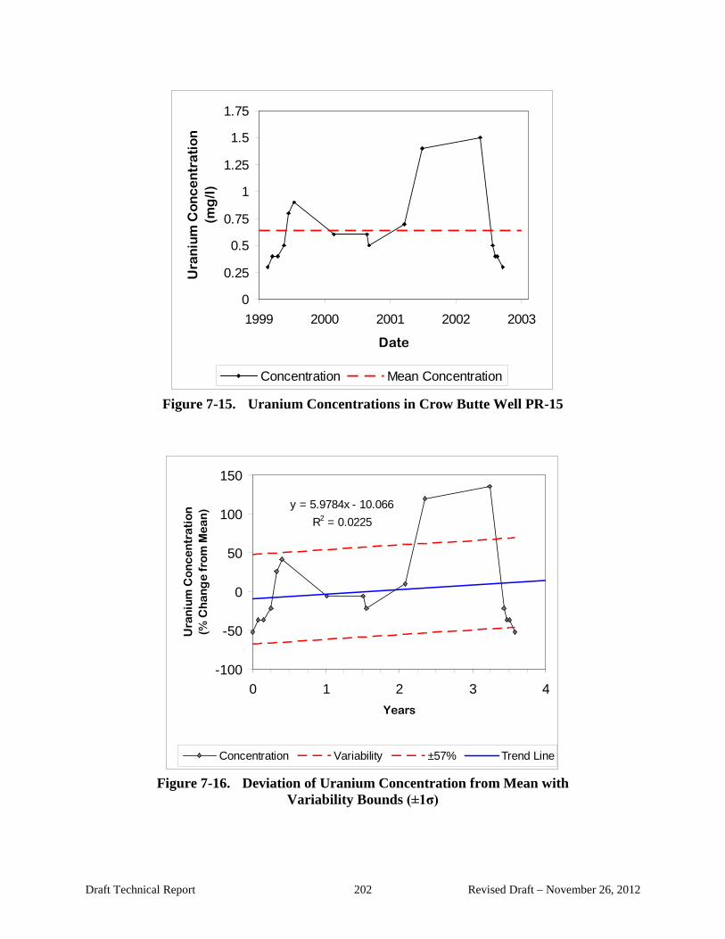
Figure 7-15. Uranium Concentrations in Crow Butte Well PR-15
1.75
on 1.5
itar 1.25
nt
eo
nc )l/ 1
gm C ( 0.75
um
ni 0.5
arU 0.25
01999 2000 2001 2002 2003
Date
Concentration Mean Concentration
Figure 7-16. Deviation of Uranium Concentration from Mean with
Variability Bounds (±1σ)
150
y = 5.9784x - 10.066
on n)
i 100 R2
t a = 0.0225
a er Mnt
e om 50
on
c r f
e C ng 0
um
ha
ni
a Cr %U ( -50
-1000 1 2 3 4
Years
Concentration Variability ±57% Trend Line
Draft Technical Report 202 Revised Draft – November 26, 2012

Figure 7-17. Radium Concentrations in Crow Butte Well PR-15
60y = -10.06x + 15.275
40 R2
on n) = 0.3154
i at ear Mn
t 20e om
on
c r f
e 0 C ng
um
i ha -20
d Ca %R ( -40
-600 1 2 3 4
Years
Concentration Variability ±27% Trend Line
Figure 7-18. Comparison of Bayesian Posterior Distributions for Regression Slope
Parameter for Uranium and Radium in Crow Butte Well PR-15
0.4
oni 0.3
but
irtsi D 0.2
oriretos 0.1
P
0-30 -20 -10 0 10 20 30 40 50
Slope (% of mean per year)
Radium (pCi/L) Uranium (mg/l)
Draft Technical Report 203 Revised Draft – November 26, 2012
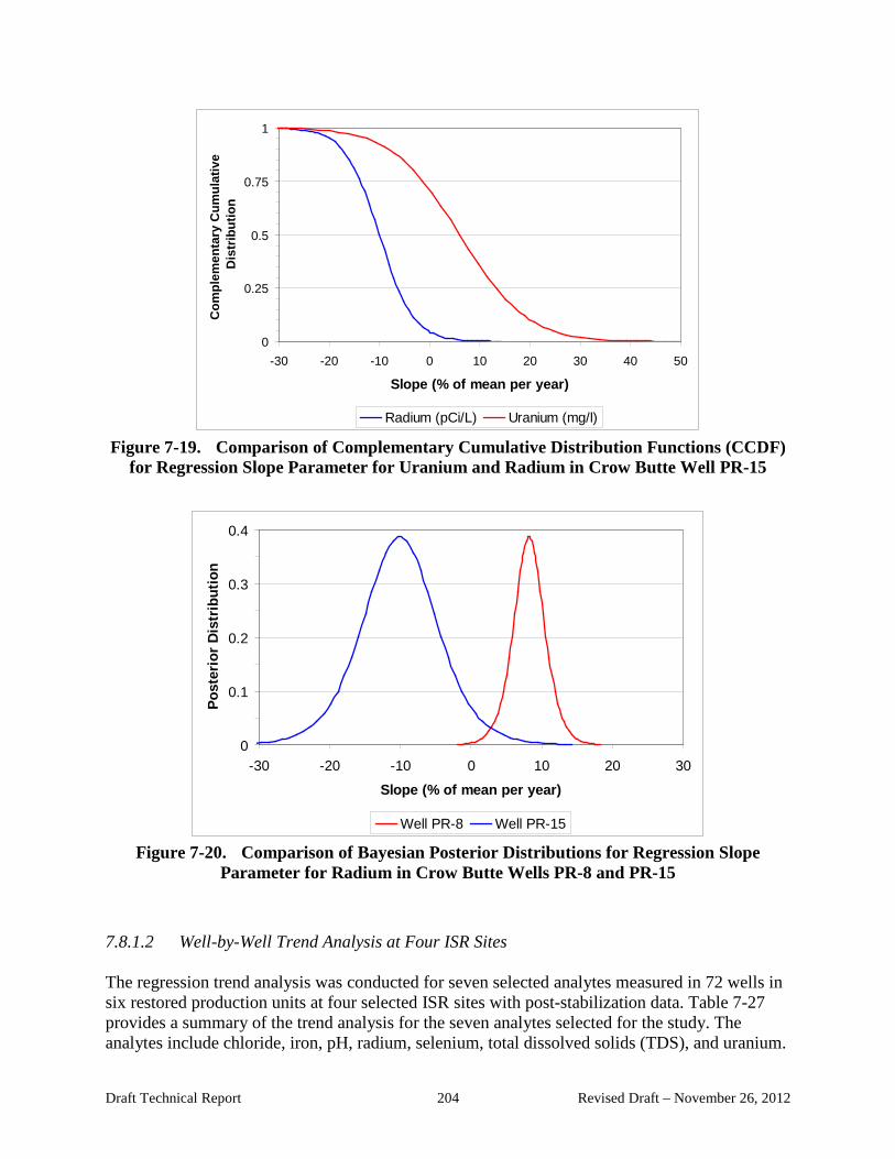
Figure 7-19. Comparison of Complementary Cumulative Distribution Functions (CCDF)
for Regression Slope Parameter for Uranium and Radium in Crow Butte Well PR-15
1
0.75
trib
utio
n0.5
ntar
y C
umul
ativ
e C
ompl
eme Dis
0.25
0-30 -20 -10 0 10 20 30 40 50
Slope (% of mean per year)
Radium (pCi/L) Uranium (mg/l)
Figure 7-20. Comparison of Bayesian Posterior Distributions for Regression Slope
Parameter for Radium in Crow Butte Wells PR-8 and PR-15
0.4
oni 0.3
but
irtsi D 0.2
oriretos 0.1
P
0-30 -20 -10 0 10 20 30
Slope (% of mean per year)
Well PR-8 Well PR-15
7.8.1.2 Well-by-Well Trend Analysis at Four ISR Sites
The regression trend analysis was conducted for seven selected analytes measured in 72 wells in six restored production units at four selected ISR sites with post-stabilization data. Table 7-27 provides a summary of the trend analysis for the seven analytes selected for the study. The analytes include chloride, iron, pH, radium, selenium, total dissolved solids (TDS), and uranium.
Draft Technical Report 204 Revised Draft – November 26, 2012
The table provides information for six regression statistics: the mean sample concentration; the number of quarters covered by the sampling program; the number of samples collected in each well; the slope of the trend line; the t-statistic for the slope; and the variability around the trend line. These results are summaries of the regressions for the number of wells shown. The table shows the minimum, maximum, mean and standard deviation for each regression statistic.
Additional details of the trend analysis are shown in Tables F-1 and F-2 in Attachment F. Table F-1 shows a summary by analyte, while Table F-2 provides details on the regressions for each analyte in each of the six production units. Table F-3 contains the trend analysis results for each well. This table contains the data that are summarized in Tables 7-21, F-1, and F-2. The table identifies the production unit, analyte, well, starting date, ending date, number of tests, R-square, variability, intercept, slope, standard error of the slope, the lower and upper bounds of the 95% confidence interval for the slope (LCL and UCL), the t-statistic for the slope, the t-test result, and the Mann-Kendall test result. The test results are recorded as a +1 if there is a significantly positive trend, -1 if there is a significantly negative trend, and 0 if the slope is not significant.
A summary of the estimated mean slope and variability is presented in Table 7-28. Figure 7-21 contains a bar plot of the mean slopes shown in Table 7-28. On average, radium, uranium and iron had positive trends, while chloride and selenium showed decreasing trends. Only chloride and uranium have a 95% confidence interval which does not include 0, indicating that only these two mean slopes are significantly different from 0.
The mean values of the variability in Table 7-28 are plotted in Figure 7-22. Iron and selenium had the highest variability, while chloride, TDS and pH show less variability. Radium and uranium are in the mid-range of variability. Figure 7-23 shows the 95% confidence interval for the mean variability of each analyte. In general, the analytes with high variability also have the widest confidence intervals. The mean variability for iron and selenium ranges from 35% to 55%, while radium and uranium have mean variability of 20% to 35%. Figure 7-24 shows the full range of variability encountered in the regression analysis. Although the confidence intervals for the mean variability are all below 55%, variability as high as 100% to 200% was encountered in individual wells.
Figure 7-25 shows a scatter plot of the standard error of the slope versus the number of samples in the regression. Most of the wells available for analysis have only 3 to 5 samples covering a period of approximately 1 year. The standard error of the slope estimates range over more than three orders of magnitude for these wells. This indicates that well-by-well trend analysis is very difficult with only 4 or 5 samples in the data set. Fewer wells were available with 7 to 10 samples, and the standard error is reduced by an order of magnitude in these wells. Only a few wells at Crow Butte were available with more than 15 samples for uranium and radium. These are the wells discussed in the introduction to this section of the report.
Draft Technical Report 205 Revised Draft – November 26, 2012

Table 7-27. Summary of Trend Analysis at Four* ISR Sites
Statistic Parameter Number of Wells Minimum Maximum Mean Standard
Deviation Mean Concentration Chloride (mg/l) 63 2.00 97.00 16.47 16.99 Iron (mg/l) 61 0.00 163.00 3.58 20.76 pH (units) 65 7.00 14.00 7.54 0.86 Radium (pCi/l) 69 23.00 3422.00 404.85 513.01 Selenium (mg/l) 49 0.00 0.00 0.02 0.05 TDS (mg/l) 72 280.00 1183.00 536.30 211.42 Uranium (mg/l) 70 0.00 9.00 1.50 1.87 Number of Quarters Chloride (mg/l) 63 2.00 5.00 2.69 0.62 Iron (mg/l) 61 1.00 14.30 3.43 3.74 pH (units) 65 1.00 5.00 2.39 1.02 Radium (pCi/l) 69 1.00 14.30 3.47 3.51 Selenium (mg/l) 49 0.00 14.30 3.84 4.05 TDS (mg/l) 72 1.30 14.00 3.61 3.22 Uranium (mg/l) 70 2.00 14.30 3.69 3.33 Number of Tests Chloride (mg/l) 63 3.00 5.00 4.24 0.59 Iron (mg/l) 61 3.00 10.00 4.18 2.00 pH (units) 65 3.00 4.00 3.62 0.49 Radium (pCi/l) 69 3.00 10.00 4.19 1.87 Selenium (mg/l) 49 3.00 10.00 5.06 1.96 TDS (mg/l) 72 3.00 9.00 4.64 1.44 Uranium (mg/l) 70 3.00 17.00 5.00 2.75 Slope of Trendline (%/y) Chloride (mg/l) 63 -139.27 315.36 -18.85 73.25 Iron (mg/l) 61 -422.10 600.91 10.10 189.99 pH (units) 65 -11.48 264.25 4.66 33.08 Radium (pCi/l) 69 -160.01 363.03 17.50 92.69 Selenium (mg/l) 49 -447.43 654.25 -12.04 187.09 TDS (mg/l) 72 -197.67 128.42 1.89 39.70 Uranium (mg/l) 70 -240.54 242.26 27.39 106.59 t-statistic Chloride (mg/l) 63 -24.38 7.64 -0.93 4.19 Iron (mg/l) 61 -7.44 25.96 0.42 4.76 pH (units) 65 -4.87 4.43 0.14 1.39 Radium (pCi/l) 69 -5.18 50.07 2.31 8.54 Selenium (mg/l) 49 -4.72 4.32 -0.34 2.19 TDS (mg/l) 72 -9.96 148.78 2.51 17.84 Uranium (mg/l) 70 -19.10 15.85 1.05 3.99 Variability (%) Chloride (mg/l) 63 1.71 74.21 15.11 11.95 Iron (mg/l) 61 3.10 211.76 44.54 40.28 pH (units) 65 0.18 99.55 4.53 12.18 Radium (pCi/l) 69 0.90 137.99 24.67 26.92 Selenium (mg/l) 49 2.50 185.67 43.97 37.08 TDS (mg/l) 72 0.07 48.07 9.53 8.83 Uranium (mg/l) 70 1.06 125.06 27.44 22.45 * Christensen, MU2 & MU3 (COGEMA 2008a), Highland A (Kearney 2004) and B
Crow Butte, MU1 (Crow Butte 2002) and Irigaray, 13 wells in 9 units (Irigaray 2004). (Power Resources 2004)),
Draft Technical Report 206 Revised Draft – November 26, 2012

Table
7-28. Mean Slope and Variability Estimates with 95% Confidence Interval for the Mean (LCL to UCL)
Slope LCL Mean UCL Chloride (mg/l) -37% -19% -1% Iron (mg/l) -38% 10% 58% pH (units) -3% 5% 13% Radium (pCi/l) -4% 17% 39% Selenium (mg/l) -64% -12% 40% TDS (mg/l) -7% 2% 11% Uranium (mg/l) 2% 27% 52% Variability LCL Mean UCL Chloride (mg/l) 12% 15% 18% Iron (mg/l) 34% 45% 55% pH (units) 2% 5% 7% Radium (pCi/l) 18% 25% 31% Selenium (mg/l) 34% 44% 54% TDS (mg/l) 7% 10% 12% Uranium (mg/l) 22% 27% 33%
Figure 7-21. Slope of Trend Line Averaged over All Wells
40%
30% 27.4%
of T
rend
line
20% 17.5%
)ye
ar 10.1%
/ 10%
ean 4.7%
Slo
pe 1.9%
mf o 0%
rage
%(
-10%
Ave -12.0%
-20% -18.9%
-30%Chloride Iron (mg/l) pH (units) Radium Selenium TDS Uranium
(mg/l) (pCi/l) (mg/l) (mg/l) (mg/l)
Analyte
Draft Technical Report 207 Revised Draft – November 26, 2012
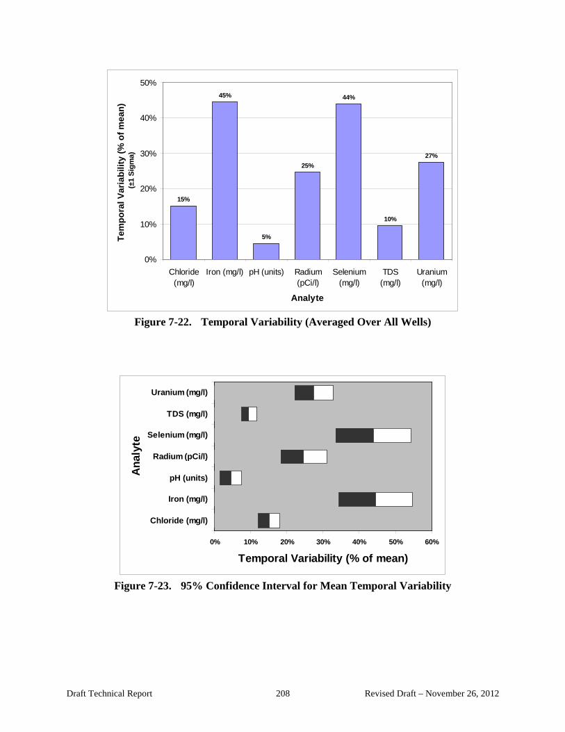
Figure 7-22. Temporal Variability (Averaged Over All Wells)
50%45% 44%
an)
bilit
y (%
of m
e 40%a) 30% 27%
mgi 25%
l Var
ia 1 S
±( 20%15%
Tem
pora
10%10%
5%
0%Chloride Iron (mg/l) pH (units) Radium Selenium TDS Uranium
(mg/l) (pCi/l) (mg/l) (mg/l) (mg/l)
Analyte
Figure 7-23. 95% Confidence Interval for Mean Temporal Variability
Uranium (mg/l)
TDS (mg/l)
e Selenium (mg/l)
ytal Radium (pCi/l)
nA pH (units)
Iron (mg/l)
Chloride (mg/l)
0% 10% 20% 30% 40% 50% 60%
Temporal Variability (% of mean)
Draft Technical Report 208 Revised Draft – November 26, 2012
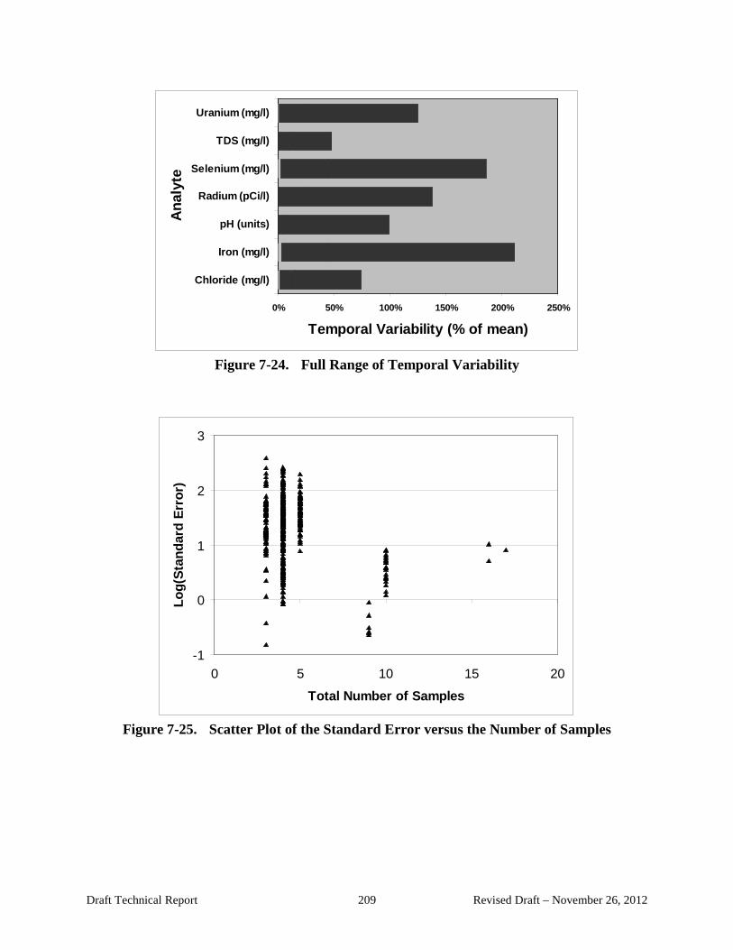
Figure 7-24. Full Range of Temporal Variability
Uranium (mg/l)
TDS (mg/l)
e Selenium (mg/l)yt
al Radium (pCi/l)n
A pH (units)
Iron (mg/l)
Chloride (mg/l)
0% 50% 100% 150% 200% 250%
Temporal Variability (% of mean)
Figure 7-25. Scatter Plot of the Standard Error versus the Number of Samples
3
)or 2
rrd
Er
nda 1
atSLo
g(
0
-10 5 10 15 20
Total Number of Samples
Draft Technical Report 209 Revised Draft – November 26, 2012

7.8.2 Pooled Trend Analysis
The trend analyses in the previous section examined over 400 time series of samples collected from a single well. It is also possible to use regression analysis to determine if samples collected from a number of wells have a significant trend. Figure 7-26 shows a scatter plot of the chloride samples collected from eight wells at Christensen Mine Unit 2. This plot uses the same scales as in the previous section, with the percentage deviation of each sample from the well mean plotted on the vertical axis and time on the horizontal axis. With data “pooled” from eight wells, this plot is an example of a pooled regression trend analysis. In a pooled analysis, data for a single analyte collected from a set of wells at all times are included in a single regression. The regression model for the pooled trend analysis is yi ,T = α + βT , where yi,T denotes the (transformed) sample value from well i at time T. Here
T=0 at the time of the earliest sample. As before, each value yi,T is a percentage deviation from the mean for that well, and time is expressed in years from the first sample. The model uses only a single coefficient for the intercept, as the mean of the percentage deviations for each well is zero, An example of a pooled regression trend line is shown in Figure 7-26. The trend line has a positive slope of 47% per year. Due to the larger number of samples available in pooled regression, the standard error of the slope estimate is greatly reduced. In this example the standard error of the slope is 11% and the t-statistic is 3.9 with 30 degrees of freedom. The t-statistic is larger than the critical value in Table 7-31 for 30 degrees of freedom. This confirms that there is a significant upward trend in the chloride measurements. The plot in Figure 7-27 shows the same data used in Figure 7-26 plotted as circles with a size proportional to the standard error of the slope estimate obtained in the trend analysis of the eight individual wells. The wells with the smallest circles had more precise estimates of their individual trends than wells with larger circles. The trends for the wells with smaller circles have trends which are near the pooled slope estimate. Figure 7-28 shows an example of the drawbacks of relying on a linear regression model to determine the trend. This plot shows the TDS samples in the same eight wells. The trend line has a positive slope of 27% with a standard error of 9.9% and a t-statistic of 2.73. Although the plot shows that concentrations increased only in the beginning and have trended down since then, the linear trend analysis concludes that there is a significant positive trend for TDS in these wells. The trend in the last 3 samples is downward. In this case, it may be necessary to redo the analysis using only the last 3 sample sets to establish the most recent trend. The standard errors of the regressions for individual wells were shown in Figure 7-29 of the previous section. The standard error ranged over several orders of magnitude in the analysis of individual wells. A similar plot of the standard errors for the pooled slope estimates is shown in Figure 7-29. The pooled sample sizes ranged from 15 to 100 depending on the production unit and analyte. The smallest pooled sample size is approximately the same as the largest individual well sample size shown in Figure 7-29. Using a pooled trend analysis, the standard errors are reduced to less than 30% when the pooled sample size is 40 or larger.
Draft Technical Report 210 Revised Draft – November 26, 2012
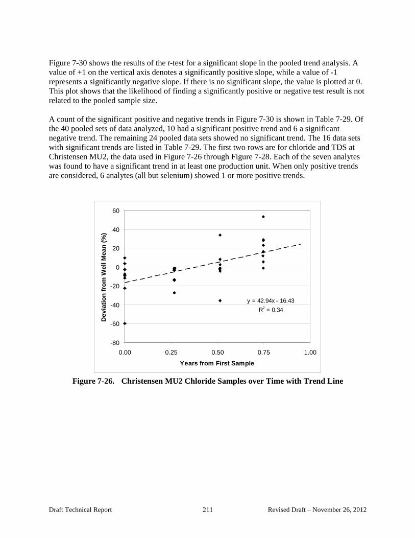
Figure 7-30 shows the results of the t-test for a significant slope in the pooled trend analysis. A value of +1 on the vertical axis denotes a significantly positive slope, while a value of -1 represents a significantly negative slope. If there is no significant slope, the value is plotted at 0. This plot shows that the likelihood of finding a significantly positive or negative test result is not related to the pooled sample size. A count of the significant positive and negative trends in Figure 7-30 is shown in Table 7-29. Of the 40 pooled sets of data analyzed, 10 had a significant positive trend and 6 a significant negative trend. The remaining 24 pooled data sets showed no significant trend. The 16 data sets with significant trends are listed in Table 7-29. The first two rows are for chloride and TDS at Christensen MU2, the data used in Figure 7-26 through Figure 7-28. Each of the seven analytes was found to have a significant trend in at least one production unit. When only positive trends are considered, 6 analytes (all but selenium) showed 1 or more positive trends.
Figure 7-26. Christensen MU2 Chloride Samples over Time with Trend Line
60
iatio
n fr
om W
ell M
ean
(%) 40
20
0
-20
y = 42.94x - 16.43-40
R2 = 0.34
Dev
-60
-800.00 0.25 0.50 0.75 1.00
Years from First Sample
Draft Technical Report 211 Revised Draft – November 26, 2012

Figure 7-27. Christensen MU2 Chloride Samples over Time with Trend Line
(Size of circle is equal to the standard error of the slope estimate for each individual well; hence, samples with smaller circles are from wells with more significant trends.)
) 75
% ( y = 42.94x - 16.43
ean 50
R2 = 0.34
Ml 25el
Wm 0
or fn -25
oiat -50
evi
D
-75-0.2 0.0 0.2 0.4 0.6 0.8 1.0
Years from First Sample
Figure 7-28. Christensen MU2 TDS Samples over Time with Trend Line
60
iatio
n fr
om W
ell M
ean
(%) 40
20
0
-20
Dev y = 27.06x - 10.36
-40R2 = 0.20
-600.00 0.25 0.50 0.75 1.00
Years from First Sample
Draft Technical Report 212 Revised Draft – November 26, 2012

Figure 7-29. Scatter Plot of Standard Error of Slope versus Pooled Number of Samples
80
ope
ld
Se 60
ool )
% P e (
of
at 40or mirr st
d E E
20
ndar
atS
00 25 50 75 100
Pooled Number of Samples
Figure 7-30. Scatter Plot of Pooled t-test Results
(+1 = significant positive trend; -1 = significant negative trend; 0 = no significant trend)
1
tles
u R
est
T- 0
tedlooP
-10 25 50 75 100
Pooled Number of Samples
t-test
Draft Technical Report 213 Revised Draft – November 26, 2012

Table 7-29. Summary of Significant Tren
Count Positive Trend 10
ds in Pooled Trend Analysis
Percent 25%
Negative Trend 6 15% No Trend 24 Total 40
60% 100%
Table 7-30. Significant Positive and Negative Trends Identified using Pooled Trend Analysis
Unit Analyte Direction Trend (%/yr) Christensen MU2 Chloride Positive 43% TDS Positive 27% pH (units) Positive 3.8% Iron Negative -124% Christensen MU3 TDS Positive 20% Iron Negative -60% Crow Butte MU1 Iron Positive 20% Uranium Positive 13% TDS Positive 2.1% Highland A Chloride Negative -69% Highland B Uranium Positive 91% Radium Positive 51% TDS Negative -13% Chloride Negative -57% Irigaray MU1-9 Iron Positive 139% Selenium Negative -108%
7.9 Verify that Contaminants and Hazardous Constituent Concentrations are Below Required Restoration Levels
This section describes traditional statistical methods for verifying that contaminants and hazardous constituent concentrations are below required restoration levels. These methods involve a comparison of well data collected in the baseline and after restoration is complete. Several types of statistical hypothesis tests are recommended for conducting this comparison. Although a geostatistical analysis is not required, these methods provide a way to convert the baseline and post-restoration sample data into 2- and 3-D graphical representations of the characteristics of the ore zone. For those operators with an understanding of geostatistical software and analytical procedures, these procedures may provide better insight into the differences between baseline characteristics and post-restoration conditions. Areas showing the greatest differences between baseline and post-restoration conditions may be identified with these procedures. Geostatistical methods and other models are useful in demonstrating that the potentiometric surface has returned to baseline conditions. This demonstration requires more than a point-by-
Draft Technical Report 214 Revised Draft – November 26, 2012
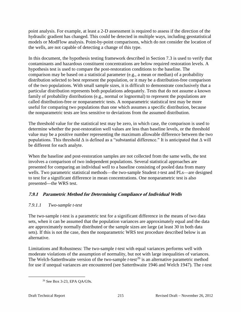
point analysis. For example, at least a 2-D assessment is required to assess if the direction of the hydraulic gradient has changed. This could be detected in multiple ways, including geostatistical models or ModFlow analysis. Point-by-point comparisons, which do not consider the location of the wells, are not capable of detecting a change of this type. In this document, the hypothesis testing framework described in Section 7.3 is used to verify that contaminants and hazardous constituent concentrations are below required restoration levels. A hypothesis test is used to compare the post-restoration conditions to the baseline. The comparison may be based on a statistical parameter (e.g., a mean or median) of a probability distribution selected to best represent the population, or it may be a distribution-free comparison of the two populations. With small sample sizes, it is difficult to demonstrate conclusively that a particular distribution represents both populations adequately. Tests that do not assume a known family of probability distributions (e.g., normal or lognormal) to represent the populations are called distribution-free or nonparametric tests. A nonparametric statistical test may be more useful for comparing two populations than one which assumes a specific distribution, because the nonparametric tests are less sensitive to deviations from the assumed distribution. The threshold value for the statistical test may be zero, in which case, the comparison is used to determine whether the post-restoration well values are less than baseline levels, or the threshold value may be a positive number representing the maximum allowable difference between the two populations. This threshold Δ is defined as a “substantial difference.” It is anticipated that Δ will be different for each analyte. When the baseline and post-restoration samples are not collected from the same wells, the test involves a comparison of two independent populations. Several statistical approaches are presented for comparing an individual well to a baseline consisting of pooled data from many wells. Two parametric statistical methods—the two-sample Student t-test and PLs—are designed to test for a significant difference in mean concentrations. One nonparametric test is also presented—the WRS test.
7.9.1 Parametric Method for Determining Compliance of Individual Wells
7.9.1.1 Two-sample t-test
The two-sample t-test is a parametric test for a significant difference in the means of two data sets, when it can be assumed that the population variances are approximately equal and the data are approximately normally distributed or the sample sizes are large (at least 30 in both data sets). If this is not the case, then the nonparametric WRS test procedure described below is an alternative. Limitations and Robustness: The two-sample t-test with equal variances performs well with moderate violations of the assumption of normality, but not with large inequalities of variances. The Welch-Satterthwaite version of the two-sample t-test26 is an alternative parametric method for use if unequal variances are encountered (see Satterthwaite 1946 and Welch 1947). The t-test
26 See Box 3-23, EPA QA/G9s.
Draft Technical Report 215 Revised Draft – November 26, 2012

is not robust against outliers because sample means and standard deviations are sensitive to outliers. The data should be screened for outliers using the method of Section 7.5.
Procedure for the Two-Sample t-Test (Equal Variances)
Step 1. Assume there are n compliance samples, X1, … Xn and N baseline samples Y1, … YN. Calculate the sample means, MX and MY, and the sample standard deviations, SX and SY of the two populations. Also compute the pooled estimate of the standard deviation using the equation:
(n − 1)S 2 + (N − 1)S 2
S p = X Y n + N + 2
M − (M + ∆)
Step 2. Compute the test statistic t = X Y0 where Δ may be 0.
1 1S p +n N
Step 3. Find the critical value of the t-distribution with degrees of freedom n+N-2 and cumulative probability (1−α) for a confidence level of 100(1−α)%, tn+N−2(1−α). The values of Student’s t-distribution are shown in Table 7-31. Step 4. If t0 > tn+N−2(1−α) then reject the null hypothesis that the true difference between population means is less than Δ.
7.9.1.2 Prediction Limit for a Future Mean
Prediction limits (PLs) are designed to provide an upper bound for the mean of a future sample with a specified probability equal to (1 - α), known as the confidence level of the PL. It represents the chance (over repeated applications of the limit to many similar data sets) that the PL will contain the mean of a future (post-operations) sample from the monitoring wells. The PL for a future mean is similar to the parametric two-sample t-test and the nonparametric WRS test, because the mean of the compliance samples is compared to a limit calculated using the baseline mean. Prediction limits (PLs) assume that the future distribution and the baseline distributions have similar shapes and differ only by a shift in concentration to a higher level. Similar assumptions apply to the other two tests. If the baseline and future distributions have significantly different shapes, then the Welch-Satterthwaite form of the (parametric) two-sample t-test and the Brunner-Munzel generalization of the (nonparametric) WRS test may exhibit better performance. A set of N baseline samples, pooled over all baseline wells and, if necessary, screened of outliers using the tolerance method described in Section 7.5, is used to construct the PL. The mean of n compliance samples from one or more wells is then compared to the PL to determine compliance. The PL has the same mathematical form as a tolerance limit, using the mean M and the standard deviation S of N baseline samples:
Draft Technical Report 216 Revised Draft – November 26, 2012

SMPL nN ⋅−+= )1(, ακ if Δ=0 or
SMPL nN ⋅−+∆+= )1(, ακ if Δ>0
Here κN,n(1 - α) is a multiplier that depends on the number of baseline samples N, the number of compliance samples n, and the desired level of confidence (1 - α).
The PL on a future mean assumes that the baseline data used to construct the limit are either normally distributed or can be normalized by a transformation. If a transformation is used (e.g., the natural logarithm) and the PL is built on the transformed values, the PL should not be back-transformed before comparing it to the compliance point data. Rather, the compliance samples should first be transformed, and the future mean computed from the transformed compliance measurements. Then the mean of the transformed values (e.g., log-mean) should be compared to the PL.
Procedure for Calculating a Prediction Limit Step 1. Calculate the sample mean M and the standard deviation S from the set of N baseline samples. Step 2. If the background data are approximately normal, calculate the PL using the equation
1 1PL = M + ∆ + t1−α ,N −1S + where Δ may be 0. n N
The Student’s t value used in the equations has degrees of freedom (N - 1) and the cumulative probability (1 - α) for a confidence level of 100(1 - α)%. The values of Student’s distribution for selected values of N - 1 are shown in Table 7-31. Step 3. Using the PL computed in Step 2, compare the mean of the compliance samples against the PL. If the future mean is below the PL, then the null hypothesis of no significant difference is accepted and compliance is indicated. If the future mean exceeds the PL, there is statistically significant evidence of an increase in concentration over baseline levels.
Table 7-31. Critical Values of the Student’s t-Distribution Degrees Confidence Level =100(1-α)%
of Freedom
90% 95% 97.5% 99% 99.5% 99.9% Probability of Exceeding Critical Value (α)
(N-1) 0.1 0.05 0.025 0.01 0.005 0.001 1 3.078 6.314 12.706 31.821 63.657 318.313 2 1.886 2.920 4.303 6.965 9.925 22.327 3 1.638 2.353 3.182 4.541 5.841 10.215 4 1.533 2.132 2.776 3.747 4.604 7.173 5 1.476 2.015 2.571 3.365 4.032 5.893 6 1.440 1.943 2.447 3.143 3.707 5.208 7 1.415 1.895 2.365 2.998 3.499 4.782
Draft Technical Report 217 Revised Draft – November 26, 2012
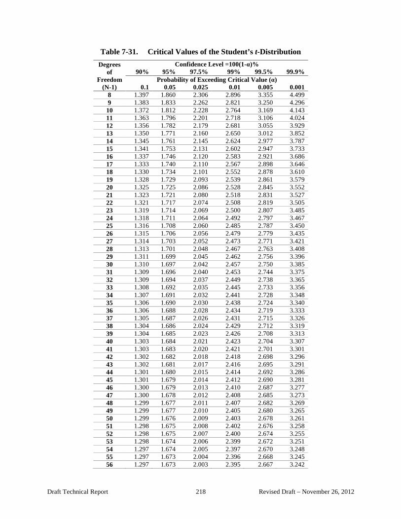
Table 7-31. Critical Values of the Student’s t-Distribution Degrees
of Freedom
(N-1)
Confidence Level =100(1-α)% 90% 95% 97.5% 99% 99.5% 99.9%
Probability of Exceeding Critical Value (α) 0.1 0.05 0.025 0.01 0.005 0.001
8 1.397 1.860 2.306 2.896 3.355 4.499 9 1.383 1.833 2.262 2.821 3.250 4.296
10 1.372 1.812 2.228 2.764 3.169 4.143 11 1.363 1.796 2.201 2.718 3.106 4.024 12 1.356 1.782 2.179 2.681 3.055 3.929 13 1.350 1.771 2.160 2.650 3.012 3.852 14 1.345 1.761 2.145 2.624 2.977 3.787 15 1.341 1.753 2.131 2.602 2.947 3.733 16 1.337 1.746 2.120 2.583 2.921 3.686 17 1.333 1.740 2.110 2.567 2.898 3.646 18 1.330 1.734 2.101 2.552 2.878 3.610 19 1.328 1.729 2.093 2.539 2.861 3.579 20 1.325 1.725 2.086 2.528 2.845 3.552 21 1.323 1.721 2.080 2.518 2.831 3.527 22 1.321 1.717 2.074 2.508 2.819 3.505 23 1.319 1.714 2.069 2.500 2.807 3.485 24 1.318 1.711 2.064 2.492 2.797 3.467 25 1.316 1.708 2.060 2.485 2.787 3.450 26 1.315 1.706 2.056 2.479 2.779 3.435 27 1.314 1.703 2.052 2.473 2.771 3.421 28 1.313 1.701 2.048 2.467 2.763 3.408 29 1.311 1.699 2.045 2.462 2.756 3.396 30 1.310 1.697 2.042 2.457 2.750 3.385 31 1.309 1.696 2.040 2.453 2.744 3.375 32 1.309 1.694 2.037 2.449 2.738 3.365 33 1.308 1.692 2.035 2.445 2.733 3.356 34 1.307 1.691 2.032 2.441 2.728 3.348 35 1.306 1.690 2.030 2.438 2.724 3.340 36 1.306 1.688 2.028 2.434 2.719 3.333 37 1.305 1.687 2.026 2.431 2.715 3.326 38 1.304 1.686 2.024 2.429 2.712 3.319 39 1.304 1.685 2.023 2.426 2.708 3.313 40 1.303 1.684 2.021 2.423 2.704 3.307 41 1.303 1.683 2.020 2.421 2.701 3.301 42 1.302 1.682 2.018 2.418 2.698 3.296 43 1.302 1.681 2.017 2.416 2.695 3.291 44 1.301 1.680 2.015 2.414 2.692 3.286 45 1.301 1.679 2.014 2.412 2.690 3.281 46 1.300 1.679 2.013 2.410 2.687 3.277 47 1.300 1.678 2.012 2.408 2.685 3.273 48 1.299 1.677 2.011 2.407 2.682 3.269 49 1.299 1.677 2.010 2.405 2.680 3.265 50 1.299 1.676 2.009 2.403 2.678 3.261 51 1.298 1.675 2.008 2.402 2.676 3.258 52 1.298 1.675 2.007 2.400 2.674 3.255 53 1.298 1.674 2.006 2.399 2.672 3.251 54 1.297 1.674 2.005 2.397 2.670 3.248 55 1.297 1.673 2.004 2.396 2.668 3.245 56 1.297 1.673 2.003 2.395 2.667 3.242
Draft Technical Report 218 Revised Draft – November 26, 2012
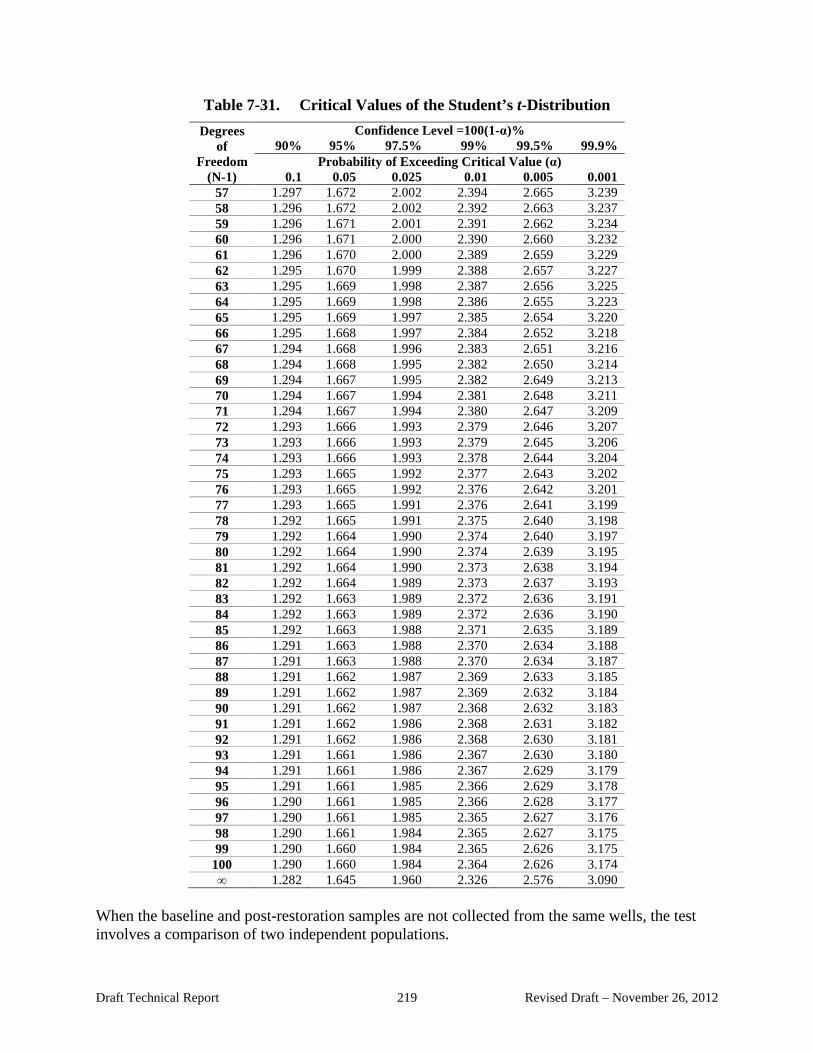
Table 7-31. Critical Values of the Student’s t-Distribution Degrees
of Freedom
(N-1)
Confidence Level =100(1-α)% 90% 95% 97.5% 99% 99.5% 99.9%
Probability of Exceeding Critical Value (α) 0.1 0.05 0.025 0.01 0.005 0.001
57 1.297 1.672 2.002 2.394 2.665 3.239 58 1.296 1.672 2.002 2.392 2.663 3.237 59 1.296 1.671 2.001 2.391 2.662 3.234 60 1.296 1.671 2.000 2.390 2.660 3.232 61 1.296 1.670 2.000 2.389 2.659 3.229 62 1.295 1.670 1.999 2.388 2.657 3.227 63 1.295 1.669 1.998 2.387 2.656 3.225 64 1.295 1.669 1.998 2.386 2.655 3.223 65 1.295 1.669 1.997 2.385 2.654 3.220 66 1.295 1.668 1.997 2.384 2.652 3.218 67 1.294 1.668 1.996 2.383 2.651 3.216 68 1.294 1.668 1.995 2.382 2.650 3.214 69 1.294 1.667 1.995 2.382 2.649 3.213 70 1.294 1.667 1.994 2.381 2.648 3.211 71 1.294 1.667 1.994 2.380 2.647 3.209 72 1.293 1.666 1.993 2.379 2.646 3.207 73 1.293 1.666 1.993 2.379 2.645 3.206 74 1.293 1.666 1.993 2.378 2.644 3.204 75 1.293 1.665 1.992 2.377 2.643 3.202 76 1.293 1.665 1.992 2.376 2.642 3.201 77 1.293 1.665 1.991 2.376 2.641 3.199 78 1.292 1.665 1.991 2.375 2.640 3.198 79 1.292 1.664 1.990 2.374 2.640 3.197 80 1.292 1.664 1.990 2.374 2.639 3.195 81 1.292 1.664 1.990 2.373 2.638 3.194 82 1.292 1.664 1.989 2.373 2.637 3.193 83 1.292 1.663 1.989 2.372 2.636 3.191 84 1.292 1.663 1.989 2.372 2.636 3.190 85 1.292 1.663 1.988 2.371 2.635 3.189 86 1.291 1.663 1.988 2.370 2.634 3.188 87 1.291 1.663 1.988 2.370 2.634 3.187 88 1.291 1.662 1.987 2.369 2.633 3.185 89 1.291 1.662 1.987 2.369 2.632 3.184 90 1.291 1.662 1.987 2.368 2.632 3.183 91 1.291 1.662 1.986 2.368 2.631 3.182 92 1.291 1.662 1.986 2.368 2.630 3.181 93 1.291 1.661 1.986 2.367 2.630 3.180 94 1.291 1.661 1.986 2.367 2.629 3.179 95 1.291 1.661 1.985 2.366 2.629 3.178 96 1.290 1.661 1.985 2.366 2.628 3.177 97 1.290 1.661 1.985 2.365 2.627 3.176 98 1.290 1.661 1.984 2.365 2.627 3.175 99 1.290 1.660 1.984 2.365 2.626 3.175
100 1.290 1.660 1.984 2.364 2.626 3.174 ∞ 1.282 1.645 1.960 2.326 2.576 3.090
When the baseline and post-restoration samples are not collected from the same wells, the test involves a comparison of two independent populations.
Draft Technical Report 219 Revised Draft – November 26, 2012

7.9.2 Nonparametric Tests for Comparing Baseline and Post-restoration Conditions
A comparison of post-restoration with baseline samples is conducted in Phase 4 to assess compliance with the baseline and in Phase 5 to determine if post-restoration values have achieved targeted remediation levels. In these comparisons, the statistical approach adopted will depend on the type of data collected.
The statistical tests are designed to compare post-restoration parameter values with baseline well parameters, assuming that both data sets were collected under stable conditions. It is likely that the baseline well data will meet this condition, except for possible seasonal effects. Before proceeding with the test for comparing baseline samples with post-restoration samples, it is first necessary to conduct the test for homogeneity of trends and for existence of a monotonic trend as described in Section 7.7.2 and in Attachment D in Boxes D-4, D-5 and D-6. These prior steps are applied to the post-restoration data to affirm stability. If the test for homogeneity of trend across wells is not met, then the individual wells should be tested for trends as described in Section 7.7.2.1 and in Attachment D in Boxes D-1, D-2 and D-3. In this case, the following procedures for determining if remediation goals are met are applicable only to the set of wells with demonstrated stability. 7.9.2.1 Comparing One Well to the Baseline A nonparametric comparison of baseline and post-restoration samples from stable wells is made using the Wilcoxon Rank Sum (WRS) test. The WRS test also is known as the Mann-Whitney or Wilcoxon-Mann-Whitney test. The advantage of using the nonparametric WRS test is that the data need not have a known distribution. Given the small sample sizes, it would be difficult to determine this distribution empirically. The WRS test also allows for nondetect measurements to be present in the baseline and/or post-restoration samples. As a general rule, the WRS test can be used with up to 40% “less than” measurements in either data set. Two assumptions underlying this test are:
(1) Samples from the baseline and post-restoration periods are independent, identically distributed random samples.
(2) Each measurement is independent of every other measurement, regardless of the set of samples from which it came.
The null hypothesis is that the post-restoration data exceed the baseline by a substantial difference. The null hypothesis is formulated for the express purpose of being rejected if the data provide support for the alternative:
• The null hypothesis (H0): The post-restoration distribution exceeds the baseline by more than Δ. Symbolically, the null hypothesis is written as H0: δ > Δ.
• The alternative hypothesis (HA): The post-restoration distribution does not exceed the baseline by more than Δ (HA: δ < Δ).
Here, Δ is the investigation level. The investigation level is determined on a case-by-case basis.
Draft Technical Report 220 Revised Draft – November 26, 2012
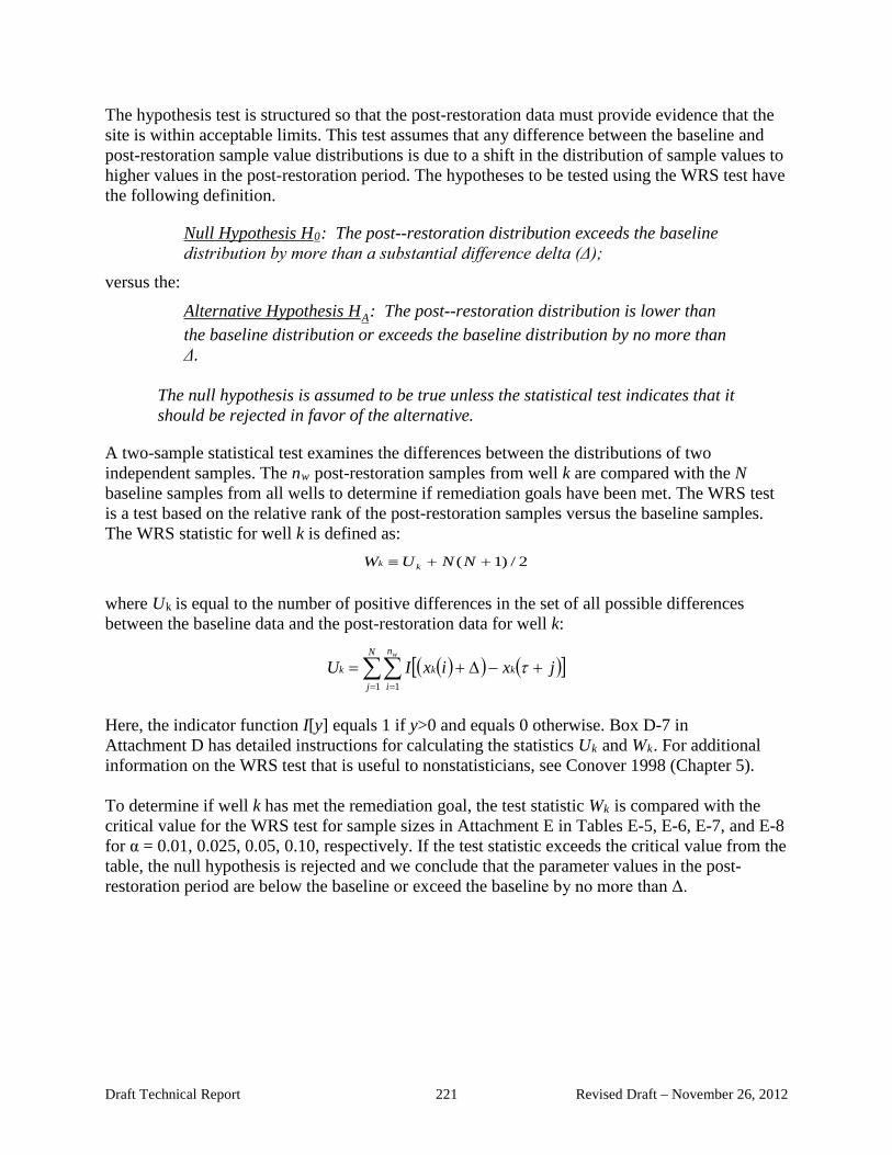
The hypothesis test is structured so that the post-restoration data must provide evidence that the site is within acceptable limits. This test assumes that any difference between the baseline and post-restoration sample value distributions is due to a shift in the distribution of sample values to higher values in the post-restoration period. The hypotheses to be tested using the WRS test have the following definition.
Null Hypothesis H0: The post--restoration distribution exceeds the baseline distribution by more than a substantial difference delta (Δ);
versus the: Alternative Hypothesis HA: The post--restoration distribution is lower than the baseline distribution or exceeds the baseline distribution by no more than Δ.
The null hypothesis is assumed to be true unless the statistical test indicates that it should be rejected in favor of the alternative.
A two-sample statistical test examines the differences between the distributions of two independent samples. The nw post-restoration samples from well k are compared with the N baseline samples from all wells to determine if remediation goals have been met. The WRS test is a test based on the relative rank of the post-restoration samples versus the baseline samples. The WRS statistic for well k is defined as:
2/)1( ++≡ NNUW kk where Uk is equal to the number of positive differences in the set of all possible differences between the baseline data and the post-restoration data for well k:
( )( ) ( )[ ]jxixIU kk
N
j
n
ik
w
+−∆+= ∑∑= =
τ1 1
Here, the indicator function I[y] equals 1 if y>0 and equals 0 otherwise. Box D-7 in Attachment D has detailed instructions for calculating the statistics Uk and Wk. For additional information on the WRS test that is useful to nonstatisticians, see Conover 1998 (Chapter 5). To determine if well k has met the remediation goal, the test statistic Wk is compared with the critical value for the WRS test for sample sizes in Attachment E in Tables E-5, E-6, E-7, and E-8 for α = 0.01, 0.025, 0.05, 0.10, respectively. If the test statistic exceeds the critical value from the table, the null hypothesis is rejected and we conclude that the parameter values in the post-restoration period are below the baseline or exceed the baseline by no more than Δ.
Draft Technical Report 221 Revised Draft – November 26, 2012

7.9.2.2 Comparing Multiple Wells: Testing for Homogeneity and Overall Compliance to the Baseline
The t-test, prediction limits and the WRS test described above are useful for analyzing the data from a single well. After a determination of compliance is made for each well, these test results may be combined to form an evaluation of compliance for the entire unit. The first step in this evaluation is to plot the test results on a map of the site using one color for wells that are determined to be in compliance and another color for the other wells. Such a plot may reveal areas where restoration has not been successful. If geostatistical software is available, indicator kriging may be used to estimate the percent of compliance throughout the unit. Hypothesis test results are used to create an indicator variable for each well. The indicator variables are 1 if in compliance and 0 if not. The resulting interpolation map would show the probabilities of compliance in all areas of the unit. The average value of this interpolated map over the entire unit provides a point estimate of the probability of compliance of the unit as a whole. This estimate of compliance has an advantage that spatial autocorrelation of the wells is accounted for explicitly in the model. However, due to the tortuous configuration of the ore zone (e,g., see Figure 7-1), estimation of the anisotropic spatial correlation structure required for such analysis may be difficult with the limited data available.
If geostatistical analysis is not available, an alternative approach is a statistical test for homogeneity. To conduct a homogeneity test for compliance, the set of test statistics Wk for all wells may be combined to make an overall summary for the entire set of wells. In this approach, the test statistics for each well Wk are used as a summary measure of compliance in each well. However, there must be consistency across wells in the relative levels of the baseline and post-restoration data to make a determination of compliance that is valid across all wells.
The procedures described in Section 7.7.2 for conducting an overall test for a trend using the summary Mann-Kendall statistics for each well may be modified to construct an overall test for determining when remediation goals are met. Two tests are used; first a test for homogeneity across wells and then a test for overall compliance. Again, both tests are based on the chi-squared distribution. The two tests are designed to be implemented sequentially, testing first for homogeneity, then for compliance across wells as follows:
Step 1. Test for comparability of wells for compliance determination
H0: Similar dynamics affect all K wells vs. HA: At least two wells exhibit different dynamics
Step 2. Test for overall compliance
H0*: Baseline values are exceeded by more than a substantial difference
Δ at one or more wells vs. HA
*: Post-restoration values are lower than baseline values or exceed baseline values by no more than a substantial difference Δ.
Draft Technical Report 222 Revised Draft – November 26, 2012
When the t-test is used to test for compliance of individual wells, the test statistic for each well k is used: zk = t0 (k) as the summary comparison statistic for each well. If the WRS test is used to determine compliance, the expected value and variance of Wk under the null distribution are:
( ) ( ) 2/1++== NnNWEE wkk ( ) ( ) 12/1++== NnNnWVarV w w
The standardized form of the test statistic Wk is zk = (Wk − Ek ) Vk . If zk is sufficiently large, there is evidence that this well has met the remediation goal. To perform the test for homogeneity (or comparability), first calculate the average of the standardized test statistics ZM = ∑Zk/K. The homogeneity chi-square statistic is χ2 2
h = (∑Z k) - KZ2
M. Using the chi-squared table in Table E-3 of Attachment E, find the critical value for χ2 with (K - 1) degrees of freedom at significance level α. For example, with a significance level of 5% and 5 degrees of freedom, χ2
(5) = 11.07; i.e., 11.07, is the cut point, which puts 5% of the probability in the upper tail of a chi-square variable with 5 degrees of freedom. If χ2
h ≤ χ2(K−1),
there are comparable test statistics across wells at significance level α. If χ2 2h > χ (K−1), the wells
are not homogeneous at the significance level α. In this case, individual α*-level tests should be conducted at each well using the methods presented in Box D-7 of Attachment D.
If the hypothesis of homogeneity across wells is accepted in Step 1, use Step 2 to affirm the compliance of all wells with the remediation goals. The chi-squared table in Table E-3 of Attachment E is used to find the critical value for χ2 with 1 degree of freedom at significance level α*. Calculate the overall compliance test statistic χ2 2 2 2 *
c = KZ M. If χ c ≥ χ (1), reject H0 and conclude that the site appears to be below baseline conditions or no more than Δ higher than baseline conditions. If χ2
c < χ2(1), there is not sufficient evidence (at the α* significance level)
that all wells are in compliance with the remediation goals. In this case, additional remediation may be required. 7.10 ProUCL Software for Statistical Analysis The ProUCL software package developed by EPA’s Technology Support Center (EPA 2010b, EPA 2010c) is designed to do many of the statistical tests/analyses recommended in this document. The technical guide to Version 4.1 of the software includes the hypothesis testing framework recommended in CERCLA guidance (EPA 2002a) and MARSSIM (EPA 2000a). These documents also were used to provide a framework for the hypothesis testing in this document, and hence all use similar notation and terminology. The package implements two of the three 2-sample tests recommended in this document for comparison with baseline (the WRS test and two-sample t-test). Each test is implemented using Test Form 1, Test Form 2 with Δ=0, and Test Form 2 with Δ>0. This fact makes the software uniquely suitable for this application. The software package also includes a sample size module for use with the parametric t-test and the WRS test. Two forms of PLs are implemented in Version 4.1, but not the PL for the future mean of k samples recommended for comparison with
kk
Draft Technical Report 223 Revised Draft – November 26, 2012
baseline in this document. The software package also contains a trend analysis module, including regression analysis, the Mann-Kendall trend test and the Thiel-Sen estimate of the slope. The package contains a variety of other parametric and nonparametric statistical methods, including modules used for plotting the data, identifying the type of probability distribution, parameter estimation and tolerance limits. Upper tolerance limits are used for determining if a future observation is a part of the distribution or not. This method may be used for outlier identification. 7.11 Summary of Statistical Approaches The statistical approaches outlined in the previous sections are summarized here. Phase 1 Baseline Sampling
• Estimate required number of baseline samples (Section 7.1).
• Adjust measured data for seasonality if required (Section 7.7.1 and Attachment D, Section D.1).
• Use regression trend test or Mann-Kendall test to check for unexpected trends (Section 7.7.2 and Attachment D, Sections D.2 and D.3).
Phase 4 Establish Compliance with Baseline
• At the end of restoration, determine the number of wells to monitor (Section 7.2) and the number of samples per well (Section 7.6) for the comparison with the baseline.
• Adjust measured individual well data for seasonality, if required (Section 7.7.1 and Attachment D, Section D.1).
• Use the two-sample t-test (Section 7.9.1.1), PLs (Section 7.9.1.2) or the WRS test (Section 7.9.2.1) to compare baseline to post-restoration conditions for each well or for pooled wells (Attachment D, Section D.4).
• For multiple wells, first test wells for homogeneity. If the hypothesis of homogeneity across all wells is accepted, then test to confirm compliance of all wells with restoration goals. (Section 7.9.2.2 and Attachment D, Section D.5).
• If steady-state data are from different wells than the baseline data and trends are not detected; use the two-sample t-test or the WRS test to compare baseline to steady-state measurements for statistical differences for the pooled data of all wells combined, which are treated as a single well. (Sections 7.9.1 and 7.9.2, and Attachment D, Section D.4).
Phase 5 Long-Term Stability Monitoring
• Determine the number of samples required to detect a trend (Section 7.7.2).
• Adjust measured data for each well for seasonality if required (Section 7.7.1 and Attachment D, Section D.1).
Draft Technical Report 224 Revised Draft – November 26, 2012

• Use the Mann-Kendall or regression trend test to test for trends for each well or in the pooled wells (Section 7.7.2 and Attachment D, Sections D.2 and D.3).
• If trend is detected, use linear regression or Theil-Sen test to assess trend magnitude (Section 7.7.2).
• Repeat for each well.
• If the before/after comparison is made between multiple wells, use the pooled-regression trend test.
Gilbert 1987 contains extensive discussions of the issues concerning use of statistics in environmental and ground water monitoring. For a detailed discussion of the tests mentioned in this chapter, as well as step-by-step guidance on calculations for the various kinds of comparisons, see also EPA 2000a and EPA 2006a.
Draft Technical Report 225 Revised Draft – November 26, 2012

8.0 SUMMARY OF POST-CLOSURE PERFORMANCE ISSUES
This section provides a synopsis of the topics discussed in the report that are important to designing a monitoring network and demonstrating acceptable postclosure performance of an in-situ mining operation.
8.1 Designing the Monitoring Program to Allow Reliable Baseline Conditions to be Established Prior to Active Mining
A meaningful interpretation of post-closure monitoring results relies on the accurate characterization of background ground water conditions before active mining (leaching) begins. The background (including determining baseline conditions in the production wellfield) monitoring program must capture both temporal and spatial variability in ground water chemistry up and down gradient from the production filed, as well as within the field. Considerations for this performance issue include:
• Placement of monitoring wells (both within and beyond the influence of the injection-withdrawal field) and well construction (e.g., screened intervals).
• Chemical constituents to be monitored, including sampling techniques, and frequencies.
• Duration of sampling to determine natural variations (and potential seasonality effects) in pre-mining ground water chemistry.
• Statistical methods for assessing variations in data and confidence measures for these data and subsequent decisions about baseline conditions (e.g., temporal variations in “background” levels and how much data are sufficient for decision making).
The placement and number of monitoring wells in and around an in-situ mining operation are strongly, if not totally, dependent on the site-specific hydrogeologic setting. The flow characteristics of the ore-bearing aquifer, the injection and withdrawal rates, and the spacing of these wells will dictate the placement of monitoring wells not only to assess baseline conditions in the aquifer, but to enable the detection of excursions of the treated ground waters beyond the wellfields.
Extensive experience in collecting and analyzing ground water chemical components exists within the technical community concerned with fate and transport of pollutants. In addition, previous investigations and restoration efforts at in-situ mining operations have produced a substantial experience base. Sampling protocols are reasonably well developed and can be reliably adapted to the in-situ mining application. The details of the sampling and analysis programs are typically defined in the operating license in agreement with the appropriate regulatory authority. We are not specifying specific requirements in detail in the Part 192 regulation, but rather deferring this responsibility to the regulatory authorities, the NRC or the States.
The mining and post-mining restoration efforts involve actively altering the chemical environment. Although reaction kinetics ultimately dictate how and over what time frames the ground water chemistry will respond, the uncertainties introduced by the heterogeneities in the
Draft Technical Report 226 Revised Draft – November 26, 2012
ore-bearing zone are complex and locally variable, which may limit the ability of predictive modeling to reliably measure system responses. Statistical assessments of ground water chemistry in monitoring well samples are the best tools for assessing the achievement of steady-state conditions. The long-term stability (many tens of years) of the restored wellfield, however, cannot be assured by only statistical analyses of relatively short-term (months to several years) of post-restoration monitoring of ground water compositions in the wellfield. Geochemical modeling of an adequately characterized rock/ground water system in the exempted aquifer offers a more reliable projection of long-term stability to be made.
Constituents to be monitored should be established on a site-specific basis. Currently, 40 CFR Part 192 requires that molybdenum and uranium be added to the list of hazardous constituents in 40 CFR 264.93,27 and Ra-226+Ra-228 (5 pCi/L) and gross alpha (15 pCi/L) have been added to the concentration limits in 40 CFR 264.94.28 NRC lists these and several additional parameters in its Standard Review Plan guidance for ISR license review (NRC 2003).
To ensure that temporal variability is captured, monitoring should be conducted over a period long enough to capture seasonal variations. Both EPA and NRC have recommended that at least four quarterly sets of samples be taken (40 CFR 264.97 and NRC 2003) to establish the background levels in (i.e., the baseline) and around the production field. Since this approach covers only one set of seasons, more samples may be required to obtain adequate statistics if seasonal variations are anticipated. If significant seasonal variations are expected, longer time frames for collecting samples sufficient to cover a number of seasonal cycles would be appropriate to establish confidence in the baseline characterization. Seasonal variations are more likely in shallow aquifers than in deeper aquifers that are more removed from recharge areas. Ground water background measurements up gradient of the production zone could be collected before and during the production phases to add to the database of information available to determine the presence or absence of seasonal variations.
Monitoring for spatial variability within the permit area for mining should include wells up gradient, down gradient, laterally adjacent to, and within the proposed leach area, sufficient to identify zones of high and low permeability. Monitoring should also include overlying and underlying aquifers, which could become contaminated from leaching activities. Offsite wells in the vicinity, such as drinking water wells and stock water wells, should also be monitored. In its Standard Review Plan for ISRs, NRC defines an acceptable set of samples as including all wellfield perimeter monitor wells, all upper and lower aquifer monitor wells, and at least one production/injection well per acre in each wellfield (except the requirement of one production well per acre can be reduced for very large wellfields). It is difficult to define minimum well spacing without detailed characterization of the flow system and injection/withdrawal rates and configuration of the mining wellfield. Here again, we are not defining detailed requirements for the number and placement of moniotoring wells. We emphasize that the pre-mining background concentrations in (i.e., the baseline) and around the production field are important input
27 40 CFR 264.93 references Appendix VIII to 40 CFR Part 261 which, in turn, lists the following inorganic species: silver, arsenic, barium, beryllium, cadmium, chromium, fluorine, mercury, nickel, lead, antimony, selenium, thallium, and V2O5.
28 In addition to Ra-226+Ra-228 and gross alpha, 40 CFR 264.94 sets specific maximum concentrations for arsenic, barium, cadmium, chromium, lead, mercury, selenium, and silver.
Draft Technical Report 227 Revised Draft – November 26, 2012
information to support the conclusion that the wellfield ground water chemistry has been restored to acceptable conditions. The pre-mining characterization of the ground water is also important to support geochemical modeling of the restored preduction field and the potential fate and transport of contaminants beyond the production field and into the down gradient portion of the exempted aquifer. We have indicated the chemical species used for geochemical modeling in previous sections of this report. Our listings of species to be monitored can be seen as a “tiering” approach, in that the top tier species are those specified in regulatory language as requirements to be met (i.e., radionuclides and toxic metals with established limits). The second tier analytes are those needed for geochemical modeling to support decisions about the long-term stability of the system and the behavior of radionuclides and toxic metals over the long term. This latter issue is particularly important to support petitions for alternate concentration limits if post-restoration activities in the production wellfield cannot reduce regulated species to acceptable levels.
8.2 Determining that the Ground Water Chemistry has Reached Steady State and Restoration Processes can be Discontinued
Regulators must receive sufficient information so that they can determine (1) that restoration is complete and steady-state conditions have been achieved before the initiation of post-restoration stability monitoring, or (2) that additional restoration efforts are necessary.
As noted in EPA 1992 (Section 7.5):
Finding that the ground water has returned to a steady state after terminating remediation efforts is an essential step in the establishment of a meaningful test of whether or not the cleanup standards have been attained. There are uncertainties in the process, and to some extent it is judgmental. However, if an adequate amount of data are carefully gathered prior to beginning remediation and after ceasing remediation, reasonable decisions can be made as to whether or not the ground water can be considered to have reached a state of stability.
The decision on whether the ground water has reached steady state will be based on a combination of statistical calculations, plots of data, ground water modeling, use of predictive models, and expert advice from hydrogeologists familiar with the site.
In addition to ground water chemistry, attention must be directed to site hydrology to establish that the potentiometric surface has returned to approximately baseline conditions.
Restoration is expected to take several years (see Table 6-1). During this time, ground water sampling will be used to follow the progress of the restoration process.
Considerations for this performance issue include:
• Placement of monitoring wells in and surrounding the injection-extraction field (proximity to the extraction field), sampling frequency, and sampling techniques (particularly if they differ from the pre-mining techniques).
Draft Technical Report 228 Revised Draft – November 26, 2012

• Chemical constituents to be examined (mobilized species) and constituents that may have been added to the ground water in attempts to restore pre-mining conditions (e.g., chemical reducing agents or other chemicals to sequester or inhibit movement of mobilized metals).
• Statistical tools necessary to determine when steady-state post-mining conditions are established (data demands and consequent uncertainty levels).
The statistical tools for assessing steady-state conditions have a well-established record of application in other contaminant remediation efforts and are easily adapted to the in-situ leaching application. In using these tools, care must be taken to ensure that the database for the site is detailed enough to allow clear application of any particular statistical method and interpretation of the results. Section 7.9 describes the statistical tools that can be used to determine steady-state conditions using both parametric and nonparametric tests. If the monitoring period is too short, divergent data reflecting slower flow paths through the ore zone, and still active chemical processes, could be missed, and an incorrect assessment of the aquifer’s chemical state could result. We are not mandating the use of any specific statistical method in the standards, however the choice of statistical methods must be appropriate to the size and quality of the database information collected, so that any regulatory decisions based upon the use of statistical measures can be justified. We anticipate that the appropriate regulatory authority will evaluate the defensibility of the choices made in the license based upon the quantity and quality of the database assembled by the facility operator.
8.3 Post-restoration Stability Monitoring
After the regulators have judged that the restoration process is complete, the period of long-term stability monitoring begins. In the past, the stability monitoring period has been set as a license condition at about 6 months, but more recently, the period has been increased to a minimum of 1 year (Table 6-1). Field experience suggests that 1 year may not be adequate. In some cases, the actual stability monitoring period has extended over several years to ensure that stability has been achieved (see Attachment B). Uranium in-situ leaching locations are typically in fluvial sandstone deposits, which exhibit lithologic heterogeneities reflecting the original depositional environments of the deposits. The formation of the uranium deposits in these sediments also introduces changes in the porosity and permeability of the ore zone in contrast to the surrounding aquifer. The mining and post-mining restoration activities would further alter the local flow regime in the ore body. In such systems, ground water flow paths through the ore body would be anticipated to differ significantly from the surrounding media, strongly suggesting that post-mining monitoring time frames should be longer than sometimes applied, in order to capture the effects of locally variable flow fields.
Considerations for this performance issue include:
• Chemical constituents in pre- and post-mining waters are examined to determine if aquifer water quality has been degraded by the leaching operations.
• Statistical measures are needed to ensure that the ground water remains stable over several years (i.e., concentrations are not trending upward).
Draft Technical Report 229 Revised Draft – November 26, 2012

• Statistical measures are needed to make decisions on whether the aquifer has achieved restoration goals.
The statistical tools that can be used for post-restoration stability monitoring are described in Section 7.8. Both parametric and nonparametric approaches are described to determine if a significant trend is occurring. The procedure involves establishing DQOs for the magnitude of the trend (%/yr) and the probability of detecting specified changes. The number of samples required then becomes a function of the variability of the actual sequential samples about the mean. As mentioned above, quantitative prediction of the ground water system’s chemical evolution is extremely difficult, and statistical measures to assess steady-state attainment remain the primary tool for evaluating the success of post-mining restoration efforts.
While statistical measures can provide confidence that the ground water chemistry has stabilized to acceptable levels within the monitoring period, these analyses do not unequivocally prove that the system will remain in that state over much longer time frames. In the process of in-situ mining, chemicals (oxidizing agents and complexing agents) were added to the ore zone to moibilize the uranium and may during that process degrade the chemical mechanism that sequestered the uranium in that location originally. The continued operation of these processes is essential to assure that the remaining uranium in the ore zone is not mobilized by oxygenated waters moving into the ore zone from the up gradient direction. Geochemical modeling using field data collected before and after the restoration process within the ore zone and down gradient from it can be used to model the chemical reducing capacity in these areas to determine if the ground water chemical system is likely to maintain chemically reducing conditions over the long term, and can provide added confidence to decisions about the stability of the restored production zone.
We have proposed several options for the length of the post-restoration stability monitoring period. The requirements of Part 192 require consistency “to the maximum extent practicable” with RCRA regulations. In RCRA regulations, a 30-year post-closure monitoring period is required before the license for a disposal facility can be terminated. The intent of that RCRA monitoring period is to provide confidence that the engineered barriers will prevent the release of contamination into the environment. We believe that the intent of ISR post-operation restoration is fundamentally the same, preventing contamination from moving into the ground water beyond the boundary of the exempted aquifer. We have proposed a number of alternatives that could be used to provide confidence that the wellfield has stabilized and will remain in that condition over the long term.
The simplest option is to establish a 30-year post-restoration monitoring period during which continued sampling would demonstrate stability within that time frame. This represents a significant lengthening of the stability monitoring period over past practices. Another alternative which would offer a mechanism to shorten the period would consist of statistically demonstrating the absence of upward trends in contaminant concentrations, and then requiring a fixed period of additional monitoring to add a measure of confidence that the chemical system is remaining stable. It is anticipated that this alternative would require less than the 30-year period while still providing some confidence that the system is maintaining stability. Another alternative to demonstrating long-term stability involves geochemical modeling to show that a
Draft Technical Report 230 Revised Draft – November 26, 2012

chemically stable environment has been established and that the reducing capacity of the system is able to maintain chemically reducing conditions over the longer term. Geochemical contaminant fate and transport modeling can also be used to support petitions for alternative concentration limits if restoration efforts fail to reduce some species to baseline levels. Such modeling could be used to demonstrate that the down gradient geochemical environment in the exempted aquifer offers the potential to reduce contaminant concentrations in the down gradient portion of the exempted aquifer. This approach is the preferred alternative presented in the proposed rulemaking.
Draft Technical Report 231 Revised Draft – November 26, 2012

9.0 REFERENCES Aagaard, P., and H.C. Helgeson, 1982. “Thermodynamic and kinetic constraints on reaction rates among minerals and aqueous solutions.” Am. J. Sci., 282, 237–285. Abdesselam, A., W. Lutze, W. Gong, E.H. Nuttall, B.A. Strietelmeir, and B.J. Travis, 1999. “Biological reduction of uranium in groundwater and subsurface soil,” Science of the Total Environment, 250 (1-3) 21-35. Air Force, 1997. “Model Field Sampling Plan,” Version 1.1. Air Force Center for Environmental Excellence, Brooks Air Force Base, Texas. Alpers, C.N., and D.K. Nordstrom, 1999. “Geochemical Modeling of Water-Rock Interactions in Mining Environments.” In: G.S. Plumlee and M.J. Logsdon (Eds.), The Environmental Geochemistry of Mineral Deposits, Part A: Processes, Techniques and Health Issues, Reviews in Economic Geology, Vol. 6A, Society of Economic Geologists, Inc., 289–324. Allison, J.D., D.S. Brown, and K.J. Novo-Gradac, 1991. MINTEQA2/PRODEFA2, A Geochemical assessment model for environmental systems: version 3.0 user’s manual. EPA/600/3-91/021. U.S. EPA, Environmental Research Laboratory, Athens, Georgia. Arbogast, L., 2011a. Letter from Larry Arbogast, Uranium One Americas, Inc., to Document Control Desk (Keith McConnell), NRC, April 19, 2011, Subject: Termination of the excursion status for monitor well 5MW 66. NRC Agencywide Documents Access and Management System (ADAMS) Accession Number: ML11116A144. Arbogast, L., 2011b. Letter from Larry Arbogast, Uranium One Americas, Inc., to Document Control Desk (Keith McConnell), NRC, July 8, 2011, Subject: Quarterly Progress Report of Monitor Wells on Excursion Status – 2nd Qtr. 2011. NRC ADAMS Accession Number: ML11196A051. ASTM (American Society for Testing and Materials) 1992. “Standard Guide for Sampling Groundwater Monitoring Wells.” Guide D4448-85a. West Conshohcken, Pennsylvania: American Society for Testing and Materials. 1992. ASTM 1998. Standard Guide for Remediation of Ground Water by Natural Attenuation at Petroleum Release Sites. Designation E1943-98. West Conshohocken, Pennsylvania. ASTM 2010. Standard Practice for Design and Installation of Groundwater Monitoring Wells. Designation D5092. West Conshohocken, Pennsylvania. Aziz, J.J., M. Vanderford, C.J. Newell, M. Ling, H.S. Rifai, and J.R. Gonzales, 2006. “Monitoring and Remediation Optimization System (MAROS) Software Version 2.2 User’s Guide.” Air Force Center for Environmental Excellence, Brooks City-Base, Texas.
Draft Technical Report 232 Revised Draft – November 26, 2012
Ball, J.W. and D.K. Nordstrom, 1991. User’s manual for WATEQ4F, with revised thermodynamic data base and test cases for calculating speciation of major, trace, and redox elements in natural waters. U.S. Geological Survey Open-File Report 91-183 (revised and reprinted August 1992).
Barcelona, M.J., 1988. “Overview of the sampling process.” In: Lawrence H. Keith (Ed.), Principles of Environmental Sampling, Chaser 1. American Chemical Society Professional Reference Book. American Chemical Society, Washington, DC, pp. 4–23, January 1988. Barcelona, M.J., and J.A. Helfrich, 1986. “Effects of well construction materials on ground water samples.” Environmental Science and Technology 20(11):1179–1184. Barcelona, M.J., and J.P. Gibb, 1986. “The development of effective ground-water sampling protocols.” In: ASTM STP-963, Proceedings of the Symposium on Field Methods for Ground Water Contamination Studies and Their Standardization for the American Society for Testing and Materials, February 2–7, 1986, Cocoa Beach, Florida, pp. 17–26. Barcelona, M.J., J.P. Gibb, and R.A. Miller, 1983. “A guide to the selection of materials for monitoring well construction and ground-water sampling.” EPA 600/S2-84-024, ISWS Contract Report 327, prepared for U.S. EPA, Robert S. Kerr Environmental Research Laboratory, Ada, Okaloma, and Environmental Monitoring Systems Laboratory, Las Vegas, Nevada. Barcelona, M.J., J.A. Helfrich, E.E. Garske, and J.P. Gibb, 1984. “A laboratory evaluation of ground-water sampling mechanisms.” Ground Water Monitoring Review 4(2):32–41. Barcelona, M.J., J.P. Gibb, J.A. Helfrich, and E.E. Garske, 1985a. “Practical guide for ground-water sampling.” EPA 600/S2-85-104, ISWS Contract Report 374, prepared for U.S. EPA, Robert S. Kerr Environmental Research Laboratory, Ada, Oklahoma, and Environmental Monitoring Systems Laboratory, Las Vegas, Nevada. Barcelona, M.J., J.A. Helfrich, and E.E. Garske, 1985b. “Sampling tubing effects on ground water samples.” Analytical Chemistry 57(2): 460–464. Barcelona, M.J., J.A. Helfrich, and E.E. Garske, 1986. “Field verification of sampling methods and materials selection for ground-water contamination studies.” In: ASTM-STP 963, Proceedings of the Symposium on Field Methods for Ground Water Contamination Studies and Their Standardization for the American Society for Testing and Materials, Cocoa Beach, Florida, February 2–7, 1986, pp. 221–231. Bethke, C.M., 1996. Geochemical Reaction Modeling. Oxford University Press, New York. Bethke, C.M., 2002. The Geochemist’s Workbench, Version 4.0: A User’s Guide to Rxn, Act2, Tact, React, and Gtplot. University of Illinois, Urbana-Champaign, Illinois. Bethke, C.M. and S. Yeakel, 2009. The Geochemist's Workbench®, Release 8.0, Reference Manual. Hydrogeology Program, University of Illinois, Urbana, Illinois.
Draft Technical Report 233 Revised Draft – November 26, 2012

Bickel, P. and K. Doksum, 2006. Mathematical Statistics, Basic Ideas and Selected Topics, 2nd Ed. Prentice Hall, Upper Saddle River, New Jersey.
Bowser, C.J., and B.F. Jones, 2002. “Mineralogic controls on the composition of natural waters dominated by silicate hydrolysis.” Am J Sci 302:582–662.
Cameco 2012. Letter from Ken Garoutte, Cameco Resources, to John Pessehl, Wyoming Department of Environmental Quality, dated August 17, 2012. Subject: Groundwater Restoration Research Proposal LQD TFN 5 1/330. Cameco Resources, Permit 633. ADAMS Accession Number: ML12235A224. Campbell, M.J., S.A. Julious, and D.G. Altman, 1995. “Estimating sample sizes for binary, ordered categorical, and continuous outcomes in two group comparisons,” BMJ. Volume 311, 28 October 1995. Charbonneau, M., 2009. “Current problems and recent advances in in-situ bioremediation of uranium-contaminated sites,” Basic Biotechnology, 5: 13-18. Charlton, S.R., C.L. Macklin, and D.L. Parkhurst, 1997. PHREEQCI—a graphical user interface for the geochemical computer program PHREEQC. U.S. Geologic Survey Water Resources Investigations Report 97–4222. Charlton, S.R., and D.L. Parkhurst, 2002. PHREEQCl–a graphical user interface to the geochemical model PHREEQC. U.S. Geologic Survey Fact Sheet FS-031-02. Christensen, S., and J. Doherty, 2008. Predictive error dependencies when using pilot points and singular value decomposition in groundwater model calibration. Advances in Water Resources. 31, 674-700. Church, C.D., R.T. Wilkin, C.N. Alpers, R.O. Rye, and R.B. McClesky, 2007. “Microbial sulfate reduction and metal attenuation in pH 4 acid mine water.” Geochemical Transactions. COGEMA 1994. Wellfield Data Package, Mine Unit 4, Christensen Ranch ISL Project. COGEMA Mining Inc. NRC ADAMS Accession Number: ML1016770445. COGEMA 1995. Wellfield Data Package, Mine Unit 5, Christensen Ranch Project. COGEMA Mining Inc. NRC ADAMS Accession Number: ML113120025. COGEMA 1996. Wellfield Data Package, Mine Unit 6, Christensen Ranch Project. COGEMA Mining Inc. NRC ADAMS Accession Number: ML101670447. COGEMA 2005. Response to LQD/DEQ, January 10, 2005, Comments: Irigaray Wellfield Restoration Report. TFN 4 1/170. NRC ADAMS Accession Number: ML053270037. COGEMA 2008a. Wellfield Restoration Report, Christensen Ranch Project, Wyoming. COGEMA Mining Inc. March 5, 2008. NRC ADAMS Accession Number: ML081060131.
Draft Technical Report 234 Revised Draft – November 26, 2012

COGEMA 2008b. Restoration Data Package, Mine Unit 5, Christensen Ranch Project. COGEMA Mining Inc. March 5, 2008. NRC ADAMS Accession Number: ML081060132. Cohen 2008. Email from Stephan Cohen, NRC, to [email protected], June 19, 2008, Subject: Documents for Crow Butte License Renewal. NRC ADAMS Accession Number: ML090580274. Colchin, M.P., L.J. Turk, and M.J. Humenick, 1978. “Sampling of ground water baseline and monitoring data for in-situ processes.” Report #EHE-78-01, CRWR157. Texas Water Resources Research Center, Austin, Texas. Conover, W.J., 1998. Practical Nonparametric Statistics, 3rd Ed. John Wiley & Sons, Inc., Hoboken, New Jersey. Cooley, R.L., 2004, A theory for modeling groundwater flow in heterogeneous media: U.S. Geological Survey Professional Paper 1679, 220 p. Crow Butte 2000. Mine Unit 1 Restoration Report, Crow Butte Uranium Project. NRC ADAMS Accession Number: ML003677938. Crow Butte 2002. Mine Unit 1 Groundwater Stability Data, Source Materials License SUA-1534, Docket Number 40-8943. Letter from Michael Griffin, Crowe Butte Resources, Inc., to Daniel Griffen, NRC. NRC ADAMS Accession Number: ML022980095. Crow Butte 2007. SUA–1535 License Renewal Application. Crawford, Nebraska.
Crow Butte 2011. Draft License Renewal for Crow Butte, SUA-1534. Docket 40-8943. 5/23/11.NRC ADAMS Accession Number: ML110760179. Davis, J.A., D.E. Meece, M. Kohler, and G.P. Curtis, 2004. “Approaches to surface complexation modeling of uranium(VI) adsorption on aquifer sediments.” Geochimica et Cosmochima Acta, 68:3621–3641. Davis, J.A., G.P. Curtis, M.J. Wilkins, M. Kohler, P.M. Fox, D.L. Naftz, and J.R. Lloyd, 2006. “Processes affecting transport of uranium in a suboxic aquifer.” Physics and Chemistry of the Earth. 31:548-555. Demuth and Schramke 2006. Fate and Transport of Post-Restoration Groundwater Constituents at In-Situ Uranium Leach Facilities, Petrotek Engineering Corporation & Enchemica LLC. Prepared for Uranium Resources, Inc. May 10, 2006. Deutsch, W.J., W.R. Martin, L.E. Eary, and R.J. Serne, 1985. Methods of Minimizing Ground-Water Contamination from In Situ Leach Uranium Mining. NUREG/CR–3709. NRC, Washington, DC. DeVoto, R.H., 1978. Uranium Geology and Exploration, Colorado School of Mines, Golden, Colorado.
Draft Technical Report 235 Revised Draft – November 26, 2012
DOE (Department of Energy) 1980. An assessment report on uranium in the United States of America: U.S. Department of Energy Report GJO-111 (80), 150 p. Doherty, J., and R.J. Hunt, 2009. “Two easily calculated statistics for evaluating parameter identifiability and error reduction.” Journal of Hydrology. 366, 119-127 Dong, W. and S. Brooks 2008. “Formation of Aqueous MgUO2(CO3)3
2- Complex and Uranium Anion Exchange onto an Exchange Resin. Environ Sci. Technol. 2008. 42, 1979-1983. Energy Metals 2007. Application for Source Material License, Moore Ranch Uranium Project. Technical Report: Volume II, Sections 2.9 through 10.3. NRC ADAMS Accession Number: ML072851268. Engesgaard, P. and K.L. Kipp, 1992. “A geochemical transport model for redox-controlled movement of mineral fronts in groundwater flow systems: a case of nitrate removal by oxidation of pyrite.” Water Resources Research 28:2829–2843. EPA (Environmental Protection Agency) 1989. Statistical Analysis of Ground-Water Monitoring Data at RCRA (Resource Conservation and Recovery Act) Facilities, Interim Final Guidance. EPA/530–SW–89–026. Washington, DC. EPA 1992. Methods for Evaluating the Attainment of Cleanup Standards, Volume 2: Ground Water, EPA/230/R-92/014. U.S. Environmental Protection Agency, Office of Policy, Planning, and Evaluation, Environmental Statistics and Information Division. Washington, DC. EPA 1999a. Use of Monitored Natural Attenuation at Superfund, RCRA Corrective Action, and Underground Storage Tank Sites, Office of Solid Waste and Emergency Response (OSWER), Directive 9200.4-17P, Final Draft. Washington, DC. Publication EPA/540/R-99/009. April 1999. EPA 1999b. Understanding Variation in Partition Coefficient, Kd, Values: Volume II: Review of Geochemistry and Available Kd Values for Cadmium, Cesium, Chromium, Lead, Plutonium, Radon, Strontium, Thorium, Tritium (3H) and Uranium. EPA 402-R-99-004B. Office of Radiation and Indoor Air, Office of Solid Waste and Emergency Response, EPA [and] Office of Environmental Restoration, U.S. Department of Energy, Washington, DC. August 1999. EPA 2000a. Multi-Agency Radiation Survey and Site Investigation Manual (MARSSIM), Revision 1. EPA/402/R-97/016. Washington, DC. EPA 2000b. Statistical Estimation and Visualization of Ground-water Contamination Data. Office of Research and Development. EPA/600/R-00/034. Washington, DC.
EPA 2000c. Policy and Program Requirements for the Mandatory Agency-Wide Quality System, EPA Order 5360.1 A2. U.S. Environmental Protection Agency. Washington, DC.
EPA 2000d. EPA Guidance for the Data Quality Objectives Process, EPA QA/G-4, EPA/600/R-96/055. U.S. Environmental Protection Agency. Washington, DC.
Draft Technical Report 236 Revised Draft – November 26, 2012

EPA 2001. EPA Requirements for Quality Assurance Project Plans, EPA QA/R-5, EPA/240/B-01/003. U.S. Environmental Protection Agency. Washington, DC.
EPA 2002a. Guidance for Comparing Background and Chemical Concentrations in Soil for CERCLA Sites. EPA 540-R-01-003/OSWER 9285.7-41. September 2002. EPA 2002b. Ground Water Issue: Calculation and Use of First-Order Rate Constants for Monitored Natural Attenuation Studies. EPA/540/S-02/500. Authors: C.J. Newell, H.S. Rifai, J.T. Wilson, J.A. Connor, J.A. Aziz, and M.P. Suarez. EPA 2002c. Workshop on Monitoring Oxidation-Reduction Processes for Ground Water Restoration, EPA/600/R-02-002. Dallas, Texas.
EPA 2002d. EPA Guidance for Quality Assurance Plans, EPA QA/G-5, EPA/240/R-02/009. U.S. Environmental Protection Agency. Washington, DC.
EPA 2002e. Guidelines for Ensuring and Maximizing the Quality, Objectivity, Utility, and Integrity of Information Disseminated by the Environmental Protection Agency, EPA/260R-02-008. U.S. Environmental Protection Agency. Washington, DC.
EPA 2006a. Data Quality Assessment: Statistical Methods for Practitioners. EPA QA/G-9S. EPA/240/B-06/003. Office of Environmental Information, Washington, DC. EPA 2006b. EPA Peer Review Handbook, 3rd ed., EPA/100/B-06/002. U.S. Environmental Protection Agency. Washington, DC. EPA 2007a. Monitored Natural Attenuation of Inorganic Contaminants in Ground Water, Vol. 1: Technical Basis for Assessment. EPA/600/R-07/139. National Risk Management Research Laboratory, Ground Water and Ecosystems Restoration Division. Ada, Oklahoma. EPA 2007b. Monitored Natural Attenuation of Inorganic Contaminants in Ground Water, Vol 2: Assessment for Non-Radionuclides Including Arsenic, Cadmium, Chromium, Copper, Lead, Nickel, Nitrate, Perchlorate, and Selenium. EPA/600/R-07/140. National Risk Management Research Laboratory, Ground Water and Ecosystems Restoration Division. Ada, Oklahoma.
EPA 2009. Statistical Analysis of Groundwater Monitoring Data at RCRA Facilities – Unified Guidance Document. EPA/530/R-09/007.
EPA 2010a. Low Stress (Low Flow) Purging and Sampling Procedure for the Collection of Ground water Samples from Monitoring Wells. EQASOP-GW 001. EPA 2010b. ProUCL Version 4.1 User Guide (Draft)- Statistical Software for Environmental Applications for Data Sets with and without Nondetect Observations. EPA/600/R-07/041. Technology Support Center, Atlanta, Georgia.
Draft Technical Report 237 Revised Draft – November 26, 2012

EPA 2010c. ProUCL Version 4.1 Technical Guide (Draft)- Statistical Software for Environmental Applications for Data Sets with and without Nondetect Observations. EPA/600/R-07/041. Technology Support Center, Atlanta, Georgia. EPA 2010d. Monitored Natural Attenuation of Inorganic Contaminants in Ground Water Volume 3: Assessment for Radionuclides Including Tritium, Radon, Strontium, Technetium, Uranium, Iodine, Radium, Thorium, Cesium, and Plutonium-Americium, National Risk Management Research Laboratory (NRMRL), Cincinnati, Ohio. Publication EPA/600/R-10/093. September 2010. EPA 2012. Letter from W. Honker, EPA's acting director of Region 6′s water quality division, to TCEQ Executive Director Zak Covar, dated May 16, 2012. Fanghänel, T., and V. Neck, 2002. “Aquatic chemistry and solubility phenomena of actinide oxides/hydroxides.” Lecture presented at the 10th International Symposium on Solubility Phenomena, Varna, Bulgaria, July 22–26, 2002. Pure Appl. Chem., Vol. 74, No. 10, pp. 1895–1907. Federal Register 2011. “Licenses, Certifications and Approvals for Materials Licenses.” Vol. 76, No. 179, pp 56951–56966. September 15, 2011. Gammons, C.G., J.J. Metesh, and D.M. Snyder, 2005. “A survey of the geochemistry of flooded mine shaft water in Butte, Montana.” Mine Water and the Environment, 25, 100–107. Gard, M., and J. Mahoney, 2012. Evaluating the Effects of Uranium Kd on the Restoration of ISL Wellfields Using PHT3D. http://www.nrc.gov/materials/uranium-recovery/public-meetings/ur-workshops/gard.pdf. Garske, E.E., and M.R. Schock, 1986. “An inexpensive flow-through cell measurement system for monitoring selected chemical parameters ground water.” Ground Water Monitoring Review 6(3):79–84. Gault, A.G., D.R. Cooke, A.T. Townsend, J.M. Charnock, and D.A. Polya, 2005. “Mechanisms of arsenic attenuation in acid mine drainage from Mount Bischoff, western Tasmania.” Science of the Total Environment, 345, 219–228. Gilbert, R.O., 1987. Statistical Methods for Environmental Pollution Monitoring. Van Nostrand Reinhold, New York. Gillham, R.W., J.L. Robin, J.F. Barker, and J.A. Cherry, 1983. Ground-water monitoring and sample bias. API Publication #4367, American Petroleum Institute, Washington, DC, June 1983. Glynn P.D., 2003. “Modeling Np and Pu transport with a surface complexation model and spatially variant sorption capacities: implications for reactive transport modeling and performance assessments of nuclear waste disposal sites.” Comput Geosci 29:331–349.
Draft Technical Report 238 Revised Draft – November 26, 2012

Griffin 2005. Letter from Michael Griffin, Crow Butte Resources, Inc., to Gary Janosko, NRC, June 16, 2005. Re: Source Materials License SUA-1534, Docket No. 40-8943, SM6-28 Monitor Well Excursion. NRC ADAMS Accession Number: ML051800471. Hall, S., 2009. Groundwater Restoration at Uranium In-Situ Recovery Mines, South Texas Coastal Plain. U.S. Geological Survey Open-File Report 2009–1143. Harbaugh, A.W., E.R. Banta, M.C. Hill, and M.G. McDonald, 2000. MODFLOW–2000, the U.S. Geological Survey Modular Ground-Water Model—User guide to modularization concepts and the ground-water flow process. U.S. Geological Survey Open-File Report 00–92. Harris, J., J.C. Loftis, and R.H. Montgomery, 1987. “Statistical methods for characterizing ground-water quality.” Ground Water 25(2): 185–193. Harshman, E.N., 1972. Geology and Uranium deposits, Shirley Basin Area, Wyoming. U.S. Geological Survey Professional Paper 745.
Harshman, E.N., 1974. “Distribution of Elements in Some Roll-Type Uranium Deposits.” In Formation of Uranium Ore Deposits—Proceedings of a Symposium, Athens, May 6–10, 1974, pp. 169–183. Hem, J.D. “Study and Interpretation of the Chemical Characteristics of Natural Water.” USGS Water Supply Paper 1473. Denver, Colorado: U.S. Geological Survey. 1970. Hem, J.D., 1985. Study and Interpretation of the Chemical Characteristics of Natural Water, 3rd Ed. USGS Water Supply Paper 2254. U.S. Geological Survey, Reston, Virginia. Hodges, J.L. Jr., and E.L. Lehman, 1956. “The Efficiency of some Nonparametric Competitors of the t-Test.” Annals of Mathematical Statistics, 27(2):324-335. Hou, B., 2004. Palaeochannel studies related to the Harris Greenstone Belt, Gawler Craton, South Australia: architecture and evolution of the Kingoonya Palaeochannel System, Report Book, 2004/1. Department of Primary Industries and Resources South Australia, Adelaide. Hoy, R.N., 2006. Baseline Ground Water Quality Conditions at In Situ Uranium Wellfields in Wyoming. Paper presented at the 2006 Billings Land Reclamation Symposium, June 4–8, 2006. Billings, Montana. http://www.asmr.us/Publications/Conference%20Proceedings/2006%20Billings/0246-Hoy-WY-1.pdf HydroGeoLogic, Inc. (2005). OU-1 Annual Ground Water Monitoring Report – Former Fort Ord, California, Appendix D: “Mann Kendall Analysis.” Ilton, E.S. et al., 2004. “Heterogeneous reduction of uranyl by micas: Crystal chemical and solution controls.” Geochimica Et Cosmochimica Acta, 68(11): 2417-2435.
Draft Technical Report 239 Revised Draft – November 26, 2012
Ilton, E.S., A. Haiduc, C.L. Cahill, A.R. Felmy, 2005. “Mica surfaces stabilize pentavalent uranium.” Inorganic Chemistry, 44(9): 2986-2988. Ilton, E.S., N.P. Qafoku, C.X. Liu, D.A. Moore, and J.M. Zachara, 2008. “Advective removal of intraparticle uranium from contaminated Vadose zone sediments,” Hanford, US. Environmental Science & Technology, 42(5): 1565-1571. Irigaray 2004. Irigaray Restoration Report, Appendix B. NRC ADAMS Accession Number: ML053270041. Jeon, B.H., B.A. Dempsey, W.D. Burgos, M.O. Barnett, and E.E. Roden, 2005. “Chemical reduction of U(VI) by Fe (II) at the solid-water interface using Natural and synthetic Fe(III) oxides,” Environmental Science and Technology, 39, 5642-5649. Johnson, R.H., and M.J. Friedel, 2009. Factoring uncertainty into restoration modeling of in-situ leach uranium mines. U.S. Geological Survey Open-File report 2009-1024. Johnson, R.H., M.I. Yoshino, S.M. Hall, and V.R. Shea, 2010. “Predictive Modeling Strategies for Operations and Closure at Uranium In-Situ Recovery Mines.” Mine Water and Innovative Thinking – IMWA 2010. Sydney, Nova Scotia. Johnson, R.H., 2011. “Reactive Transport Modeling for the Proposed Dewey Burdock Uranium In-Situ Recovery Mine, Edgemont, South Dakota, USA.” Presented at the IMWA 11th International Mine Water Association Congress, Mine Water – Managing the Challenges, Aachen, Germany. Kearney 2004. Letter from W.F. Kearney, Power Resources, to Gary Janosko, NRC. RE: Smith Ranch-Highland Uranium Project, Docket No. 408964, SUA-1548, A-Wellfield Ground Water Restoration Information. NRC ADAMS Accession Number: ML040300369. Koretsky, C. (2000). “The significance of surface complexation reactions in hydrologic systems: a geochemist's perspective.” 1. Hydrol. 230, 127 -171. Langmuir, D., 1997. Aqueous Environmental Geochemistry. Prentice Hall, Upper Saddle River, New Jersey. Lasaga A.C., 1981. “Transition state theory,” in Kinetics of Geochemical Processes, A.C. Lasaga and R.J. Kirkpatrick (Eds.). Rev. in Mineralogy 8, pp. 135–69, Min. Soc. Am. Leach 2001. Letter from M. Leach, NRC, to M. Griffin, Crow Butte Resources, Inc., June 26, 2001. Subject: License Amendment 11, Crow Butte Resources In Situ Leach Facility, License No. SUA-1534. Lee, S.Y., M.H. Baik, and J.W. Choi, 2010. “Biogenic Formation and Growth of Uraninite (UO2).” Environ. Sci. Technol. 44, 8409-8414.
Draft Technical Report 240 Revised Draft – November 26, 2012
Liggett, W.S., 1984. “Detecting elevated contamination by comparison with background.” In: G.E. Schweitzer and J.A. Santoluci (Eds.), Environmental Sampling for Hazardous Wastes, Chapter 13. American Society Symposium Series #267, pp. 119–128,Washington, DC.
Liggett, W.S., 1985. “Statistical aspects of designs for studying sources of contamination in quality assurance for environmental measurements.” In: J.K. Taylor and T.W. Stanley (Eds.), ASTM STP 867. American Society for Testing and Materials, Philadelphia, Pennsylvania, pp. 22–40. Liu C., J. Zachara, L. Zhong, S. Heald, Z. Wang, B. Jeon, and J.K. Fredrickson, 2009. “Microbial reduction of intragrain U(VI) in contaminated sediment.” Environmental Science and Technology, 434928-4933. Loftis, J.C., R.H. Montgomery, J. Harris, D. Nettles, P.S. Porter, R.C. Ward, and T.G. Sanders, 1986. “Monitoring strategies for ground-water quality management.” Final report, USGS Grant 14-08-0001-G-1060, Colorado Water Resources Research Institute, Fort Collins, Colorado. Long, P.E., S.B. Yabusaki, P.D. Meyer, C.L. Murray, and A.L. N’Guessan, 2008. Technical Basis for Assessing Uranium Bioremediation Performance, NUREG-CR-6973, U.S. Nuclear Regulatory Commission.
Maest, A.S., and J.R. Kuipers, 2005. “Predicting Water Quality at Hardrock Mines: Methods and Models, Uncertainties and State-of-the-Art.” Earthworks. Washington, DC.
Malapai 1988. Christensen Ranch Production Unit 3, Baseline Water Quality Data Package. Willow Creek Satellite, Phase 1. Malapai Resources Company.
Martin, J., G. Wiatzka, J. Scharer, and B. Halbert, 2005. “Case Studies that Illustrate the Benefits, Limitations and Information Requirements of Geochemical Modelling.” In Proceedings of the 12th Annual British Columbia – MEND ARD/Ml Workshop, November 30 and December 1, Vancouver, British Columbia. Mayer, K.U., E.O. Frind, and D.W. Blowes, 2002. “Multicomponent reactive transport modeling in variably saturated porous media using a generalized formulation for kinetically controlled reactions.” Water Resources Research, 38, 1174, doi: 10:1029/2001WR000862. Mayer, K.U., D.W. Blowes, and E.O. Frind, 2003. “Advances in Reactive-Transport Modeling of Contaminant Release and Attenuation from Mine-Waste Deposits.” In J.L. Jambor, D.W. Blowes and A.I.M. Ritchie (Eds.), Environmental Aspects of Mine Wastes, Short Course Series, Vol. 31, Mineralogical Association of Canada, 283–302. Meyer, P.D., M. Ye, M.L. Rockhold, S.P. Neuman, and K.J. Cantrell, 2007. Combined Estimation of Hydrogeologic Conceptual Model, Parameter, and Scenario Uncertainty with Application to Uranium Transport at the Hanford Site 300 Area, NUREG/CR-6940, U.S. Nuclear Regulatory Commission, Washington, DC.
Draft Technical Report 241 Revised Draft – November 26, 2012
McKinley, J.P., J.M. Zachara, J. Wan, D.E. McCready, and S.M. Heald, 2007. “Geochemical controls on contaminant uranium in vadose Hanford Formation sediments at the 200 Area and 300 Area, Hanford Site, Washington.” Vadose Zone Journal, 6:1004-1017. Misra, K.C., 2000. Understanding Mineral Deposits, 845 pp. Dordrecht, Netherlands: Kluwer Academic. Moncur, M.C., C.J. Ptacek, D.W. Blowes, and J.L. Jambor, 2005. “Release, transport and attenuation of metals from an old tailings impoundment.” Applied Geochemistry, 20, 639–659.
Montgomery, R.H., J.C. Loftis, and J. Harris, 1987. “Statistical characteristics of ground water quality variables.” Ground Water 25(2):176-184.
Moon, H.S., P.R. Komolos, and P.R. Jaffe, 2009. “Biogenic U(IV) oxidation by dissolved oxygen and nitrate in sediment after prolonged U(VI)/Fe(III)/SO4
-2 reduction,” Journal of Contaminant Hydrology, 105;18-27. Moss, M.E., D.P. Lettenmaier, and E.F. Wood, 1978. “On the design of hydrologic data networks.” EOS-Transactions of the American Geophysical Union 59(8):772–775.
Murakami, T., T. Sato, T. Ohnuki, and H. Isobe, 2005. “Field evidence for uranium nanocrystallization and its implications for uranium transport.” Chemical Geology, 221:117–126. Newell, C.J., S.K. Farhat, P.C. de Blanc, and J.R. Gonzales, 2002. BIOSOURCE Source Attenuation Decision Support System and Database. Air Force Center for Environmental Excellence, Brooks Air Force Base, Texas.
NFESC 2000. Guide to Optimal Ground water Monitoring – Interim Final. Naval Facilities Engineering Service Center, Port Hueneme, California. NMA (National Mining Association) 2007. Generic Environmental Report in Support of the Nuclear Regulatory Commission’s Generic Environmental Impact Statement for In Situ Uranium Recovery Facilities. Nordstrom, D.K., and C.N. Alpers, 1999. “Geochemistry of acid mine waters.” In G.S. Plumlee, and M.J. Logsdon (Eds.), The Environmental Geochemistry of Mineral Deposits, 6A, pp. 133–160. Society of Economic Geologists, Littleton, Colorado. NRC 1997. Final Environmental Impact Statement to Construct and Operate the Crownpoint Uranium Solution Mining Project, Crownpoint, New Mexico. NUREG-1508. U.S. Nuclear Regulatory Commission, Washington, DC.
NRC 1998. Environmental Assessment for Renewal of Source Material License No. SUA-1534 – Crow Butte Resources Incorporated, Crow Butte Uranium Project Dawes County, Nebraska. Docket No. 40-8943. U.S. Nuclear Regulatory Commission, Washington, DC. NRC ADAMS Accession Number: ML071520242.
Draft Technical Report 242 Revised Draft – November 26, 2012

NRC 2001. A Baseline Risk-Informed Performance-Based Approach for In-Situ Leach Uranium Extraction Licensees. NUREG/CR–6733, U.S. Nuclear Regulatory Commission, Washington, DC. NRC ADAMS Accession Number: ML012840152. NRC 2003. Standard Review Plan for In Situ Leach Uranium Extraction License Applications. Final Report. NUREG-1569. Prepared by J. Lusher. U.S. Nuclear Regulatory Commission, Washington, DC. NRC ADAMS Accession Number: ML032250177. NRC 2006. Groundwater Quality Monitoring Issues at In Situ Leach (ISL), Author P. Michalak Facilities; June 28, 2006. NRC ADAMS Accession Number: ML061910547. NRC 2007. Consideration of Geochemical Issues in Ground water Restorations at Uranium In-Situ Leach Mining Facilitie. NUREG/CR-6870. Authors: J.A. Davis and G.P. Curtis. U.S. Nuclear Regulatory Commission, Washington, DC. NRC ADAMS Accession Number: ML070600405. NRC 2009. Generic Environmental Impact Statement for In-Situ Leach Uranium Milling Facilities. NUREG-1910, Final Report. U.S. Nuclear Regulatory Commission, Washington, DC. NRC 2010. Environmental Impact Statement for the Moore Ranch ISR Project in Campbell County, Wyoming. Supplement to the Generic Environmental Impact Statement for In-Situ Leach Uranium Milling Facilities, Final Report. NUREG-1910, Supplement 1. U.S. Nuclear Regulatory Commission, Washington, DC. NRC ADAMS Accession Number: ML102290470. NRC 2011a. Environmental Impact Statement for the NIchols Ranch ISR Project in Campbell and Johnson Counties, Wyoming. NUREG-1910 Supplement 2. U.S. Nuclear Regulatory Commission, Washington, DC. January 2011. NRC ADAMS Accession Number: ML103440120. NRC 2011b. Environmental Impact Statement for the Lost Creek ISR Project in Sweetwater County, Wyoming. NUREG-1910 Supplement 3. U.S. Nuclear Regulatory Commission, Washington, DC. June 2011. NRC ADAMS Accession Number: ML11125A006. NRDC (National Resources Defense Council) 2012. Nuclear Fuel’s Dirty Beginnings. G.H. Fettus and M.G. McKinzie (auth.). March 2012. Ochs, M., J.A. Davis, M. Olin, T.E. Payne, C.J. Tweed, M.M. Askarieh, and S. Altmann, 2006. “Use of thermodynamic sorption models to derive radionuclide Kd values for performance assessment: selected results and recommendations of the NEA sorption project.” Radiochimica Acta, 94:779–785. Odeh, R.E., and D.B. Owen, 1980. Tables for Normal Tolerance Limits, Sampling Plans, and Screening. Marcel Dekker, Inc., New York.
Draft Technical Report 243 Revised Draft – November 26, 2012

O’Loughlin, E.J., S.D. Kelly, R.E. Cook, R. Csencsits, and K.M. Kemner, 2003. “Reduction of Uranium(VI) by mixed iron(II/iron(III) hydroxide (green rust): Formation of UO2 manoparticies.” Environ. Sci. Technol. 37, 721-727. Ortiz-Bernard, I., R.T. Anderson, H.A. Vironis, and D.R. Lovely, 2004. “Resistance of solid-phaseU(IV) to microbial reduction during in situ bioremediation of uranium-contaminated ground water,” Applied and Environmental Microbiology, 70 (12),(7558-7560).
Parkhurst, D.L., L.N. Plummer, and D.C. Thorstenson, 1982. BALANCE – a computer program for calculating mass transfer for geochemical reactions in ground water. U.S. Geological Survey Water Resources Investigations Report 82-14. Parkhurst, D.L., 1995. Users guide to PHREEQC − A computer program for speciation, reaction-path, advective-transport, and inverse geochemical calculations. U.S. Geological Survey, Water Resources Investigations Report 95-4227. Parkhurst, D.L., and C.A.J. Appelo, 1999. User’s guide to PHREEQC (Version2) – A computer program for speciation, batch-reaction, one-dimensional transport, and inverse geochemical calculations. U.S. Geological Survey Water Resources Investigations Report 99-4259. Parkhurst, D.L., K.L. Kipp, P. Engesgaard, and S.R. Charlton, 2004. PHAST—A program for simulating ground-water flow, solute transport, and multicomponent geochemical reactions. U.S. Geological Survey Techniques and Methods 6-A8. Parkhurst, D.L., K.L. Kipp, and S.R. Charlton, 2010. PHAST version 2 – A program for simulating ground water flow, solute transport, and multicomponent geochemical reactions. U.S. Geological Survey Techniques and Methods 6-A35. Payne, T.E., and P.L. Airey, 2006. “Radionuclide migration at the Koongarra uranium deposit, Northern Australia – Lessons from the Alligator Rivers analogue project.” Physics and Chemistry of the Earth, 31:572-586. Pearson , F.J. Junior, C.J. Noronha, and R.W. Anderson, 1983. “Mathematical modeling of the distribution of natural 14C, 234U, and 238U in a regional ground-water system”, Radiocarbon, 35: 291-300. Perkins, E.H., Y.K. Kharaka, W.D. Gunter, and J. D. DeBraal, 1990. Chapter 9, pp. 117–127, Chapter DOI: 10.1021/bk-1990-0416.ch009, ACS Symposium Series, Vol. 416. ISBN13: 9780841217294eISBN: 9780841212725. December 7, 1990. Copyright © 1990 American Chemical Society. Pitzer, K.S., 1979. “Theory − Ion interaction approach.” In R.M. Pytkowitcz (Ed.), Activity Coefficients in Electrolyte Solutions, Vol. 1, pp. 157–208. CRC Press, Inc., Boca Raton, Florida. Plummer, L.N., and D.L. Parkhurst, 1990. “Application of the Pitzer Equations to the PHREEQE geochemical model.” In D.C. Melchior and R.L. Bassett (Eds.), Chemical modeling of aqueous
Draft Technical Report 244 Revised Draft – November 26, 2012

systems II: American Chemical Society Symposium Series 416, pp. 128–137. American Chemical Society, Washington, DC. Plummer, L.N., E.C. Prestemon, and D.L. Parkhurst, 1994. An interactive code (NETPATH) for modeling NET geochemical reactions along a flow PATH—Version 2.0. U.S. Geological Survey Water Resources Investigations Report 94-4169. Pollock, D.W., 1994. User’s Guide for MODPATH/MODPATH-PLOT, Version 3: A particle tracking post-processing package for MODFLOW, the U. S. Geological Survey finite-difference ground-water flow model. U.S. Geological Survey Open-File Report 94-464. Porter, K.S., and N.M. Trautman, 1984. Seasonality in ground water quality. Draft report by Cornell University Center for Environment Research for the U.S. Environmental Protection Agency, Environmental Modeling Systems Laboratory, Las Vegas, Nevada. Power Resources 2004. Mine Unit B Ground Water Restoration Report, Smith Ranch – Highland Uranium Project. NRC ADAMS Accession Number: ML091831100. Powertech 2009. Dewey-Burdock Project Application for NRC Uranium Recovery License, Fall River and Custer Counties, South Dakota Technical Report. NRC ADAMS Accession Number: ML092870295. Prommer, H., 2002. “A Reactive Multicomponent Transport Model for Saturated Porous Media, User’s Manual Version 1.0.” Contaminated Land Assessment and Remediation Research Centre, The University of Edinburgh, United Kingdom. Puls, R.W. and M.J. Barcelona, 1989. Ground Water Sampling for Metals Analyses. Superfund Ground Water Issue. EPA/540/4-89/001. March 1989. Puls, R.W. and M.J. Barcelona, 1996. Low-Flow (Minimal Drawdown) Ground-Water Sampling Procedure, EPA/540/S-95/504, 12 pp. Reisinger, H.J., D.R. Burris, and J.G. Hering, 2005. “Remediating subsurface arsenic contamination with monitored natural attenuation.” Environmental Science and Technology 39: 458A–464A. Rojas, J.L., 1989. “Introduction to in situ leaching of uranium.” In-Situ Leaching of Uranium: Technical, Environmental, and Economic Aspects. IAEA–TECDOC–492. International Atomic Energy Agency. Vienna, Austria. Sanders, T.G., R.C. Ward, J.C. Loftis, T.D. Steel, D.D. Adrian, and V.Yevjevich, 1983. “Design of networks for monitoring water quality.” Water Resources Publications. Littleton, Colorado. Sass, Ronald L. 2011. Uranium Mining in Texas: Why Is It Done That Way? James A. Baker III Institute for Public Policy, Rice University. http://bakerinstitute.org/publications/GCC-pub-SassUraniumMining-032811.pdf
Draft Technical Report 245 Revised Draft – November 26, 2012
Sato, T., T. Murakami, N. Yanase, H. Isobe, T.E. Payne, and P.L. Airey, 1997. “Iron nodules scavenging uranium from ground water.” Environmental Science and Technology, 31:2854–2858. Satterthwaite, F. E., 1946. "An Approximate Distribution of Estimates of Variance Components." Biometrics Bulletin 2: 110–114, DOI:10.2307/3002019. SC&A 2011. Groundwater Modeling Studies at In Situ Leaching Facilities and Evaluation of Doses And Risks to Off-Site Receptors from Contaminated Groundwater. EPA Work Assignment 2-06, Task 2. December 2011. Schmidt, C., 1989. “Groundwater Restorations and Stabilization at the Ruth-ISL Test Site In Wyoming, USA.” In Situ Leaching of Uranium: Technical, Environmental and Economic Aspects. IAEA-TECDOC-492. International Atomic Energy Agency. Vienna, Austria. Sowder, A.G., P.M. Bertsch, and P.J. Morris, 2003. “Partitioning and availability of uranium and nickel in contaminated riparian sediments.” Journal of Environmental Quality, 32:885–898.
Sposito, G., and J. Coves, 1988. SOILCHEM: A computer program for the calculation of chemical spcciation in soils. Keamey Found. Soil Sci., University of California, Riverside, California. SRK 2011. Powertech Uranium Corporation, NI 43-101 Preliminary Assessment Dewey Burdock Project. SRK Consulting. Updated February 7, 2011. http://www.sedar.com/CheckCode.do;jsessionid=0000bPJAOqWov6XP6tTk_Wd_ECu:-1 Staub, W.P., N.E. Hinkle, R.E. Williams, F. Anastasi, J. Oslensky, and D. Rogruss, 1986. An Analysis of Excursions at Selected In Situ Uranium Mines in Wyoming and Texas. NUREG/CR-3967. U.S. Nuclear Regulatory Commission. Washington, DC.
Steefel, C.I., 2009. CrunchFlow: Software for Modeling Multicomponent Reactive Flow and Transport. User’s Manual. October 12, 2009. Strata Energy 2010. Ross ISR Project U.S. NRC License Application, Crook County Wyoming. NRC ADAMS Accession Number: ML110130335. TCEQ 2010. Groundwater Classification. TCEQ Regulatory Guidance, Remediation Division, RG-366/TRPP-8, Revised March 2010. http://www.tceq.texas.gov/publications/rg/rg-366_trrp_08.html.
Teahon 2005a. Letter from Larry Teahon, Crow Butte Resources, Inc., to Gary Janosko, NRC, November 14, 2005. Re: Source Materials License SUA-1534, Docket No. 40-8943, CM9-16 Monitor Well Excursion. NRC ADAMS Accession Number: ML053270239. Teahon 2005b. Letter from Larry Teahon, Crow Butte Resources, Inc., to Gary Janosko, NRC, July 15, 2005. Re: Source Materials License SUA-1534, Docket No. 40-8943, SM6-28 Monitor Well Excursion. NRC ADAMS Accession Number: ML052220108.
Draft Technical Report 246 Revised Draft – November 26, 2012

Teahon 2006a. Letter from Larry Teahon, Crow Butte Resources, Inc., to Gary Janosko, NRC, April 7, 2006. Re: Source Materials License SUA-1534, Docket No. 40-8943, CM8-21 Monitor Well Excursion. NRC ADAMS Accession Number: ML061220279 Teahon 2006b. Letter from Larry Teahon, Crow Butte Resources, Inc., to Gary Janosko, NRC, October 2, 2006. Re: Source Materials License SUA-1534, Docket No. 40-8943, PR-15 Monitor Well Excursion. NRC ADAMS Accession Number: ML06860036. Thorstenson, D.C., and D.L. Parkhurst, 2002. Calculation of individual isotope equilibrium constants for implementation in geochemical models. U.S. Geologic Survey Water Resource Investigations Report 02-4172. Thorstenson, D.C. and D.L.Parkhurst, 2004. “Calculation of individual isotope equilibrium constants for geochemical reactions.” Geochim Cosmochim Acta 68(11):2449–2465 Todd, D.K., R.M. Tinlin, K.D. Schmidt, and L.G. Everett, 1976. Monitoring ground water quality: monitoring methodology. EPA 600/4-76-026. U.S. Environmental Protection Agency, Environmental Monitoring Systems Laboratory, Las Vegas, Nevada. Total Resources, 1993. Wellfield Data Package, Unit 2 North, Christensen Ranch Project, WDEQ Permit to Mine No. 478. NRC ADAMS Accession Number: ML101670446. Um, W., R.J. Serne, C.F. Brown, and G.V. Last, 2007. “U(VI) adsorption on aquifer sediments at the Hanford Site.” Journal of Contaminant Hydrology 93:255–269. URI (Uranium Resources Inc.) 2006. Fate and Transport of Post-Restoration Groundwater Constituents at In-Situ Uranium Leach Facilities. Petrotek and Enchemica. URI (Uranium Resources Inc.) 2010. Restoration La Rosita Mine, Duval County Texas. Uranium Resources, Inc. NRC/NMA Uranium Recovery Workshop, May 27, 2010. Wan, J., T. Tokunaga, E. Brodie, Z. Wang, Z. Zheng, D. Herman, T. Hazen, M. Firestone, and S. Sutton, 2005. “Reoxidation of Bioreduced Uranoum under Reducing Conditions.” Environ. Sci. Technol. 39, 6162-6169. Welch, B. L., 1947. “The generalization of ‘Student's’ problem when several different population variances are involved,” Biometrika 34: 28–35. Wichers, D., 2006. Email from Donna Wichers, COGEMA, to Ron Linton, NRC, August 11, 2006. RE: Request: Summary Table Irigarary Mine Unit Restoration RAI response. NRC ADAMS Accession Number: ML062400363. Wolery, T.J., 1992. EQ3/6, A Computer Program for Geochemical Aqueous Speciation-Solubility Calculations: Theoretical Manual, User’s Guide, and Related Documentation (Version 7.0). UCRL-MA-11066, Pt Ill. Lawrence Livermore National Laboratory. Livermore, California.
Draft Technical Report 247 Revised Draft – November 26, 2012
Yabusaki, S.B., Y. Fang, and S. Waichler, 2008. “Building conceptual models of field-scale uranium reactive transport in a dynamic vadose zone-aquifer-river system.” Water Resources Research. Yabusaki, S.B., Y. Fang, S.R. Waichler, and P.E. Long, 2010. Processes, Properties, and Conditions Controlling In Situ Bioremediation of Uranium in Shallow, Alluvial Aquifers, NUREG/CR-7014, U.S. Nuclear Regulatory Commission. Yeskis, D. and B. Zavala, 2002. Ground-Water Sampling Guidelines for Superfund and RCRA Project Managers. EPA 542-S-02-001. May 2002. Yue, S., and P. Pilon, 2004. “A comparison of the power of the t-test, Mann-Kendall and bootstrap tests for trend detection.” Hydrological Sciences, 49(1). Zheng, C., and P.P.Wang, 1999. “MT3DMS: A modular three-dimensional multispecies transport model formulation of advection, dispersion, and chemical reactions of contaminants in groundwater systems; documentation and user’s guide.” Contract Report SERDP-99-1, U.S. Army Engineer Research and Development Center, Vicksburg, Mississippi.
Draft Technical Report 248 Revised Draft – November 26, 2012