4 Recurrences
14
4 Recurrences As noted in Section 2.3.2, when an algorithm contains a recursive call to itself, its running time can often be described by a recurrence. A recurrence is an equation or inequality that describes a function in terms of its value on smaller inputs. For example, we saw in Section 2.3.2 that the worst-case running time T (n ) of the MERGE-S ORT procedure could be described by the recurrence T (n ) = (1) if n = 1 , 2T (n /2) + (n ) if n > 1 , (4.1) whose solution was claimed to be T (n ) = (n lg n ). This chapter offers three methods for solving recurrences—that is, for obtain- ing asymptotic “” or “ O ” bounds on the solution. In the substitution method, we guess a bound and then use mathematical induction to prove our guess correct. The recursion-tree method converts the recurrence into a tree whose nodes represent the costs incurred at various levels of the recursion; we use techniques for bound- ing summations to solve the recurrence. The master method provides bounds for recurrences of the form T (n ) = aT (n /b) + f (n ), where a ≥ 1, b > 1, and f (n ) is a given function; it requires memorization of three cases, but once you do that, determining asymptotic bounds for many simple recurrences is easy. Technicalities In practice, we neglect certain technical details when we state and solve recur- rences. A good example of a detail that is often glossed over is the assumption of integer arguments to functions. Normally, the running time T (n ) of an algorithm is only defined when n is an integer, since for most algorithms, the size of the input is always an integer. For example, the recurrence describing the worst-case running time of MERGE-S ORT is really
-
Upload
khangminh22 -
Category
Documents
-
view
1 -
download
0
Transcript of 4 Recurrences
4 Recurrences
As noted in Section 2.3.2, when an algorithm contains a recursive call to itself, itsrunning time can often be described by a recurrence. A recurrence is an equationor inequality that describes a function in terms of its value on smaller inputs. Forexample, we saw in Section 2.3.2 that the worst-case running time T (n) of theMERGE-SORT procedure could be described by the recurrence
T (n) =!!(1) if n = 1 ,2T (n/2) + !(n) if n > 1 ,
(4.1)
whose solution was claimed to be T (n) = !(n lg n).This chapter offers three methods for solving recurrences—that is, for obtain-
ing asymptotic “!” or “O” bounds on the solution. In the substitution method, weguess a bound and then use mathematical induction to prove our guess correct. Therecursion-tree method converts the recurrence into a tree whose nodes representthe costs incurred at various levels of the recursion; we use techniques for bound-ing summations to solve the recurrence. The master method provides bounds forrecurrences of the form
T (n) = aT (n/b) + f (n),
where a ! 1, b > 1, and f (n) is a given function; it requires memorization ofthree cases, but once you do that, determining asymptotic bounds for many simplerecurrences is easy.
Technicalities
In practice, we neglect certain technical details when we state and solve recur-rences. A good example of a detail that is often glossed over is the assumption ofinteger arguments to functions. Normally, the running time T (n) of an algorithm isonly defined when n is an integer, since for most algorithms, the size of the input isalways an integer. For example, the recurrence describing the worst-case runningtime of MERGE-SORT is really
4.1 The substitution method 63
T (n) =!!(1) if n = 1 ,T (!n/2") + T (#n/2$) + !(n) if n > 1 .
(4.2)
Boundary conditions represent another class of details that we typically ignore.Since the running time of an algorithm on a constant-sized input is a constant,the recurrences that arise from the running times of algorithms generally haveT (n) = !(1) for sufficiently small n. Consequently, for convenience, we shallgenerally omit statements of the boundary conditions of recurrences and assumethat T (n) is constant for small n. For example, we normally state recurrence (4.1)as
T (n) = 2T (n/2) + !(n) , (4.3)
without explicitly giving values for small n. The reason is that although changingthe value of T (1) changes the solution to the recurrence, the solution typicallydoesn’t change by more than a constant factor, so the order of growth is unchanged.
When we state and solve recurrences, we often omit floors, ceilings, and bound-ary conditions. We forge ahead without these details and later determine whetheror not they matter. They usually don’t, but it is important to know when they do.Experience helps, and so do some theorems stating that these details don’t affectthe asymptotic bounds of many recurrences encountered in the analysis of algo-rithms (see Theorem 4.1). In this chapter, however, we shall address some of thesedetails to show the fine points of recurrence solution methods.
4.1 The substitution method
The substitution method for solving recurrences entails two steps:
1. Guess the form of the solution.
2. Use mathematical induction to find the constants and show that the solutionworks.
The name comes from the substitution of the guessed answer for the function whenthe inductive hypothesis is applied to smaller values. This method is powerful, butit obviously can be applied only in cases when it is easy to guess the form of theanswer.
The substitution method can be used to establish either upper or lower boundson a recurrence. As an example, let us determine an upper bound on the recurrence
T (n) = 2T (#n/2$) + n , (4.4)
which is similar to recurrences (4.2) and (4.3). We guess that the solution is T (n) =O(n lg n). Our method is to prove that T (n) % cn lg n for an appropriate choice of

64 Chapter 4 Recurrences
the constant c > 0. We start by assuming that this bound holds for !n/2", that is,that T (!n/2") # c !n/2" lg(!n/2"). Substituting into the recurrence yields
T (n) # 2(c !n/2" lg(!n/2")) + n
# cn lg(n/2) + n
= cn lg n $ cn lg 2 + n
= cn lg n $ cn + n# cn lg n ,
where the last step holds as long as c % 1.Mathematical induction now requires us to show that our solution holds for the
boundary conditions. Typically, we do so by showing that the boundary condi-tions are suitable as base cases for the inductive proof. For the recurrence (4.4),we must show that we can choose the constant c large enough so that the boundT (n) # cn lg n works for the boundary conditions as well. This requirementcan sometimes lead to problems. Let us assume, for the sake of argument, thatT (1) = 1 is the sole boundary condition of the recurrence. Then for n = 1, thebound T (n) # cn lg n yields T (1) # c1 lg 1 = 0, which is at odds with T (1) = 1.Consequently, the base case of our inductive proof fails to hold.
This difficulty in proving an inductive hypothesis for a specific boundary condi-tion can be easily overcome. For example, in the recurrence (4.4), we take advan-tage of asymptotic notation only requiring us to prove T (n) # cn lg n for n % n0,where n0 is a constant of our choosing. The idea is to remove the difficult bound-ary condition T (1) = 1 from consideration in the inductive proof. Observe thatfor n > 3, the recurrence does not depend directly on T (1). Thus, we can replaceT (1) by T (2) and T (3) as the base cases in the inductive proof, letting n0 = 2.Note that we make a distinction between the base case of the recurrence (n = 1)and the base cases of the inductive proof (n = 2 and n = 3). We derive from therecurrence that T (2) = 4 and T (3) = 5. The inductive proof that T (n) # cn lg nfor some constant c % 1 can now be completed by choosing c large enough so thatT (2) # c2 lg 2 and T (3) # c3 lg 3. As it turns out, any choice of c % 2 suffices forthe base cases of n = 2 and n = 3 to hold. For most of the recurrences we shallexamine, it is straightforward to extend boundary conditions to make the inductiveassumption work for small n.
Making a good guess
Unfortunately, there is no general way to guess the correct solutions to recurrences.Guessing a solution takes experience and, occasionally, creativity. Fortunately,though, there are some heuristics that can help you become a good guesser. Youcan also use recursion trees, which we shall see in Section 4.2, to generate goodguesses.
4.1 The substitution method 65
If a recurrence is similar to one you have seen before, then guessing a similarsolution is reasonable. As an example, consider the recurrence
T (n) = 2T (!n/2" + 17) + n ,
which looks difficult because of the added “17” in the argument to T on the right-hand side. Intuitively, however, this additional term cannot substantially affect thesolution to the recurrence. When n is large, the difference between T (!n/2") andT (!n/2"+17) is not that large: both cut n nearly evenly in half. Consequently, wemake the guess that T (n) = O(n lg n), which you can verify as correct by usingthe substitution method (see Exercise 4.1-5).
Another way to make a good guess is to prove loose upper and lower boundson the recurrence and then reduce the range of uncertainty. For example, we mightstart with a lower bound of T (n) = !(n) for the recurrence (4.4), since we have theterm n in the recurrence, and we can prove an initial upper bound of T (n) = O(n2).Then, we can gradually lower the upper bound and raise the lower bound until weconverge on the correct, asymptotically tight solution of T (n) = "(n lg n).
Subtleties
There are times when you can correctly guess at an asymptotic bound on the so-lution of a recurrence, but somehow the math doesn’t seem to work out in the in-duction. Usually, the problem is that the inductive assumption isn’t strong enoughto prove the detailed bound. When you hit such a snag, revising the guess bysubtracting a lower-order term often permits the math to go through.
Consider the recurrence
T (n) = T (!n/2") + T (#n/2$) + 1 .
We guess that the solution is O(n), and we try to show that T (n) % cn for anappropriate choice of the constant c. Substituting our guess in the recurrence, weobtain
T (n) % c !n/2" + c #n/2$ + 1= cn + 1 ,
which does not imply T (n) % cn for any choice of c. It’s tempting to try a largerguess, say T (n) = O(n2), which can be made to work, but in fact, our guess thatthe solution is T (n) = O(n) is correct. In order to show this, however, we mustmake a stronger inductive hypothesis.
Intuitively, our guess is nearly right: we’re only off by the constant 1, a lower-order term. Nevertheless, mathematical induction doesn’t work unless we prove theexact form of the inductive hypothesis. We overcome our difficulty by subtractinga lower-order term from our previous guess. Our new guess is T (n) % cn & b,
66 Chapter 4 Recurrences
where b ! 0 is constant. We now have
T (n) " (c #n/2$ % b) + (c &n/2' % b) + 1= cn % 2b + 1" cn % b ,
as long as b ! 1. As before, the constant c must be chosen large enough to handlethe boundary conditions.
Most people find the idea of subtracting a lower-order term counterintuitive. Af-ter all, if the math doesn’t work out, shouldn’t we be increasing our guess? The keyto understanding this step is to remember that we are using mathematical induc-tion: we can prove something stronger for a given value by assuming somethingstronger for smaller values.
Avoiding pitfalls
It is easy to err in the use of asymptotic notation. For example, in the recur-rence (4.4) we can falsely “prove” T (n) = O(n) by guessing T (n) " cn andthen arguing
T (n) " 2(c #n/2$) + n
" cn + n
= O(n) , () wrong!!
since c is a constant. The error is that we haven’t proved the exact form of theinductive hypothesis, that is, that T (n) " cn.
Changing variables
Sometimes, a little algebraic manipulation can make an unknown recurrence simi-lar to one you have seen before. As an example, consider the recurrence
T (n) = 2T (#*n$) + lg n ,
which looks difficult. We can simplify this recurrence, though, with a change ofvariables. For convenience, we shall not worry about rounding off values, suchas
*n, to be integers. Renaming m = lg n yields
T (2m) = 2T (2m/2) + m .
We can now rename S(m) = T (2m) to produce the new recurrence
S(m) = 2S(m/2) + m ,
which is very much like recurrence (4.4). Indeed, this new recurrence has thesame solution: S(m) = O(m lg m). Changing back from S(m) to T (n), we obtainT (n) = T (2m) = S(m) = O(m lg m) = O(lg n lg lg n).
4.2 The recursion-tree method 67
Exercises
4.1-1Show that the solution of T (n) = T (!n/2") + 1 is O(lg n).
4.1-2We saw that the solution of T (n) = 2T (#n/2$)+ n is O(n lg n). Show that the so-lution of this recurrence is also !(n lg n). Conclude that the solution is "(n lg n).
4.1-3Show that by making a different inductive hypothesis, we can overcome the dif-ficulty with the boundary condition T (1) = 1 for the recurrence (4.4) withoutadjusting the boundary conditions for the inductive proof.
4.1-4Show that "(n lg n) is the solution to the “exact” recurrence (4.2) for merge sort.
4.1-5Show that the solution to T (n) = 2T (#n/2$ + 17) + n is O(n lg n).
4.1-6Solve the recurrence T (n) = 2T (
%n) + 1 by making a change of variables. Your
solution should be asymptotically tight. Do not worry about whether values areintegral.
4.2 The recursion-tree method
Although the substitution method can provide a succinct proof that a solution toa recurrence is correct, it is sometimes difficult to come up with a good guess.Drawing out a recursion tree, as we did in our analysis of the merge sort recurrencein Section 2.3.2, is a straightforward way to devise a good guess. In a recursiontree, each node represents the cost of a single subproblem somewhere in the set ofrecursive function invocations. We sum the costs within each level of the tree toobtain a set of per-level costs, and then we sum all the per-level costs to determinethe total cost of all levels of the recursion. Recursion trees are particularly usefulwhen the recurrence describes the running time of a divide-and-conquer algorithm.
A recursion tree is best used to generate a good guess, which is then verifiedby the substitution method. When using a recursion tree to generate a good guess,you can often tolerate a small amount of “sloppiness,” since you will be verifyingyour guess later on. If you are very careful when drawing out a recursion tree andsumming the costs, however, you can use a recursion tree as a direct proof of a
68 Chapter 4 Recurrences
solution to a recurrence. In this section, we will use recursion trees to generategood guesses, and in Section 4.4, we will use recursion trees directly to prove thetheorem that forms the basis of the master method.
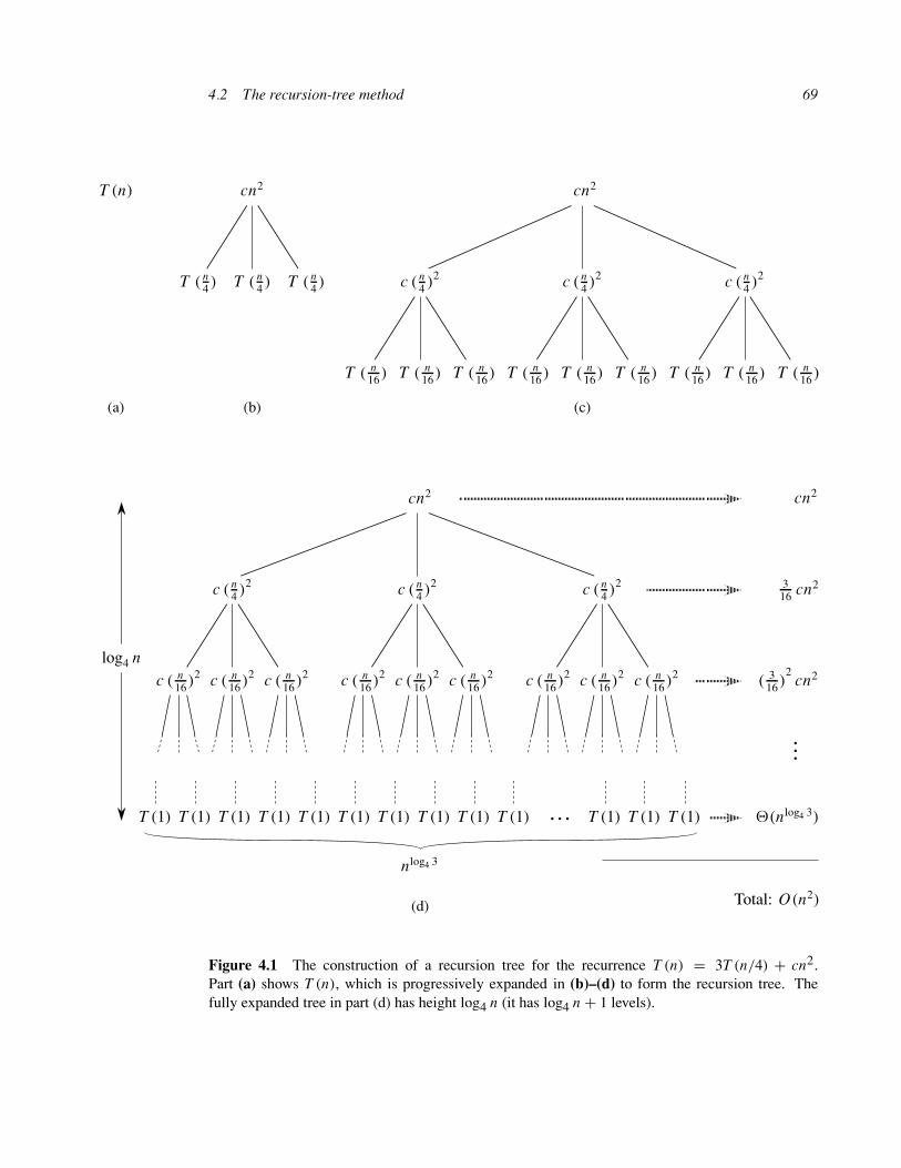
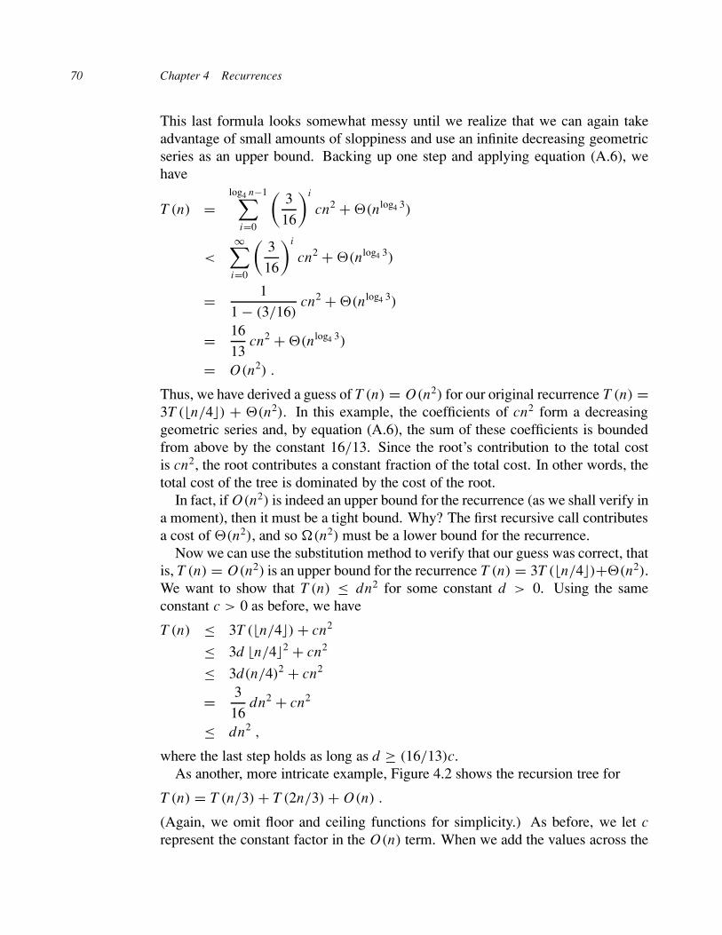
For example, let us see how a recursion tree would provide a good guess forthe recurrence T (n) = 3T (!n/4") + !(n2). We start by focusing on finding anupper bound for the solution. Because we know that floors and ceilings are usuallyinsubstantial in solving recurrences (here’s an example of sloppiness that we cantolerate), we create a recursion tree for the recurrence T (n) = 3T (n/4) + cn2,having written out the implied constant coefficient c > 0.
Figure 4.1 shows the derivation of the recursion tree for T (n) = 3T (n/4)+ cn2.For convenience, we assume that n is an exact power of 4 (another example oftolerable sloppiness). Part (a) of the figure shows T (n), which is expanded inpart (b) into an equivalent tree representing the recurrence. The cn2 term at theroot represents the cost at the top level of recursion, and the three subtrees of theroot represent the costs incurred by the subproblems of size n/4. Part (c) showsthis process carried one step further by expanding each node with cost T (n/4)from part (b). The cost for each of the three children of the root is c(n/4)2. Wecontinue expanding each node in the tree by breaking it into its constituent parts asdetermined by the recurrence.
Because subproblem sizes decrease as we get further from the root, we eventu-ally must reach a boundary condition. How far from the root do we reach one? Thesubproblem size for a node at depth i is n/4i . Thus, the subproblem size hits n = 1when n/4i = 1 or, equivalently, when i = log4 n. Thus, the tree has log4 n + 1levels (0, 1, 2, . . . , log4 n).
Next we determine the cost at each level of the tree. Each level has three timesmore nodes than the level above, and so the number of nodes at depth i is 3i .Because subproblem sizes reduce by a factor of 4 for each level we go downfrom the root, each node at depth i , for i = 0, 1, 2, . . . , log4 n # 1, has a costof c(n/4i)2. Multiplying, we see that the total cost over all nodes at depth i ,for i = 0, 1, 2, . . . , log4 n # 1, is 3i c(n/4i)2 = (3/16)i cn2. The last level, atdepth log4 n, has 3log4 n = nlog4 3 nodes, each contributing cost T (1), for a total costof nlog4 3T (1), which is !(nlog4 3).
Now we add up the costs over all levels to determine the cost for the entire tree:
T (n) = cn2 + 316
cn2 +!
316
"2
cn2 + · · · +!
316
"log4 n#1
cn2 + !(nlog4 3)
=log4 n#1#
i=0
!3
16
"i
cn2 + !(nlog4 3)
= (3/16)log4 n # 1(3/16) # 1
cn2 + !(nlog4 3) .
4.2 The recursion-tree method 69
……
(d)
(c)(b)(a)
T (n) cn2 cn2
cn2
T ( n4 )T ( n
4 )T ( n4 )
T ( n16)T ( n
16)T ( n16)T ( n
16)T ( n16)T ( n
16)T ( n16)T ( n
16)T ( n16)
cn2
c ( n4 )2c ( n
4 )2c ( n4 )2
c ( n4 )2c ( n
4 )2c ( n4 )2
c ( n16)
2c ( n16)
2c ( n16)
2c ( n16)
2c ( n16)
2c ( n16)
2c ( n16)
2c ( n16)
2c ( n16)
2
316 cn2
( 316)
2cn2
log4 n
nlog4 3
T (1)T (1)T (1)T (1)T (1)T (1)T (1)T (1)T (1)T (1)T (1)T (1)T (1) !(nlog4 3)
Total: O(n2)
Figure 4.1 The construction of a recursion tree for the recurrence T (n) = 3T (n/4) + cn2.Part (a) shows T (n), which is progressively expanded in (b)–(d) to form the recursion tree. Thefully expanded tree in part (d) has height log4 n (it has log4 n + 1 levels).
70 Chapter 4 Recurrences
This last formula looks somewhat messy until we realize that we can again takeadvantage of small amounts of sloppiness and use an infinite decreasing geometricseries as an upper bound. Backing up one step and applying equation (A.6), wehave
T (n) =log4 n!1!
i=0
"3
16
#i
cn2 + !(nlog4 3)
<"!
i=0
"3
16
#i
cn2 + !(nlog4 3)
= 11 ! (3/16)
cn2 + !(nlog4 3)
= 1613
cn2 + !(nlog4 3)
= O(n2) .
Thus, we have derived a guess of T (n) = O(n2) for our original recurrence T (n) =3T (#n/4$) + !(n2). In this example, the coefficients of cn2 form a decreasinggeometric series and, by equation (A.6), the sum of these coefficients is boundedfrom above by the constant 16/13. Since the root’s contribution to the total costis cn2, the root contributes a constant fraction of the total cost. In other words, thetotal cost of the tree is dominated by the cost of the root.
In fact, if O(n2) is indeed an upper bound for the recurrence (as we shall verify ina moment), then it must be a tight bound. Why? The first recursive call contributesa cost of !(n2), and so "(n2) must be a lower bound for the recurrence.
Now we can use the substitution method to verify that our guess was correct, thatis, T (n) = O(n2) is an upper bound for the recurrence T (n) = 3T (#n/4$)+!(n2).We want to show that T (n) % dn2 for some constant d > 0. Using the sameconstant c > 0 as before, we have
T (n) % 3T (#n/4$) + cn2
% 3d #n/4$2 + cn2
% 3d(n/4)2 + cn2
= 316
dn2 + cn2
% dn2 ,
where the last step holds as long as d & (16/13)c.As another, more intricate example, Figure 4.2 shows the recursion tree for
T (n) = T (n/3) + T (2n/3) + O(n) .
(Again, we omit floor and ceiling functions for simplicity.) As before, we let crepresent the constant factor in the O(n) term. When we add the values across the
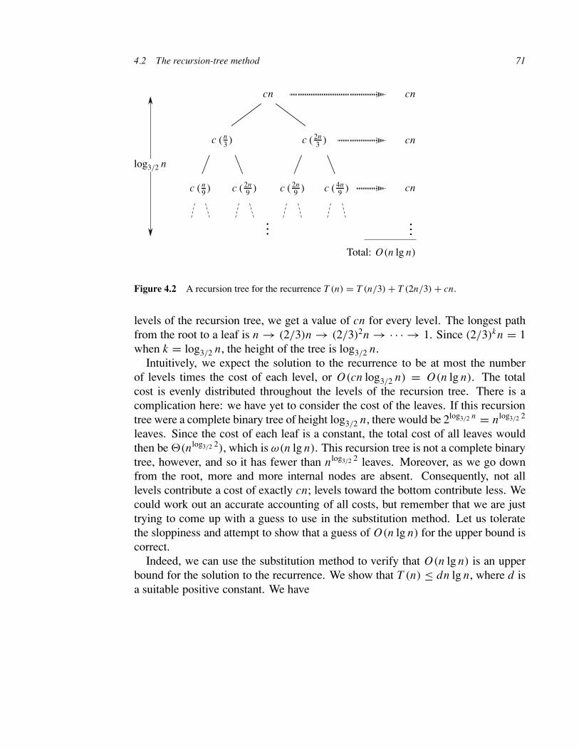
4.2 The recursion-tree method 71
… …
cn
cn
cn
cn
c (n3 ) c ( 2n
3 )
c (n9 ) c ( 2n
9 )c ( 2n9 ) c ( 4n
9 )
log3/2 n
Total: O(n lg n)
Figure 4.2 A recursion tree for the recurrence T (n) = T (n/3) + T (2n/3) + cn.
levels of the recursion tree, we get a value of cn for every level. The longest pathfrom the root to a leaf is n ! (2/3)n ! (2/3)2n ! · · · ! 1. Since (2/3)kn = 1when k = log3/2 n, the height of the tree is log3/2 n.
Intuitively, we expect the solution to the recurrence to be at most the numberof levels times the cost of each level, or O(cn log3/2 n) = O(n lg n). The totalcost is evenly distributed throughout the levels of the recursion tree. There is acomplication here: we have yet to consider the cost of the leaves. If this recursiontree were a complete binary tree of height log3/2 n, there would be 2log3/2 n = nlog3/2 2
leaves. Since the cost of each leaf is a constant, the total cost of all leaves wouldthen be !(nlog3/2 2), which is "(n lg n). This recursion tree is not a complete binarytree, however, and so it has fewer than nlog3/2 2 leaves. Moreover, as we go downfrom the root, more and more internal nodes are absent. Consequently, not alllevels contribute a cost of exactly cn; levels toward the bottom contribute less. Wecould work out an accurate accounting of all costs, but remember that we are justtrying to come up with a guess to use in the substitution method. Let us toleratethe sloppiness and attempt to show that a guess of O(n lg n) for the upper bound iscorrect.
Indeed, we can use the substitution method to verify that O(n lg n) is an upperbound for the solution to the recurrence. We show that T (n) " dn lg n, where d isa suitable positive constant. We have
72 Chapter 4 Recurrences
T (n) ! T (n/3) + T (2n/3) + cn
! d(n/3) lg(n/3) + d(2n/3) lg(2n/3) + cn
= (d(n/3) lg n " d(n/3) lg 3)
+ (d(2n/3) lg n " d(2n/3) lg(3/2)) + cn= dn lg n " d((n/3) lg 3 + (2n/3) lg(3/2)) + cn
= dn lg n " d((n/3) lg 3 + (2n/3) lg 3 " (2n/3) lg 2) + cn
= dn lg n " dn(lg 3 " 2/3) + cn
! dn lg n ,
as long as d # c/(lg 3 " (2/3)). Thus, we did not have to perform a more accurateaccounting of costs in the recursion tree.
Exercises
4.2-1Use a recursion tree to determine a good asymptotic upper bound on the recurrenceT (n) = 3T ($n/2%) + n. Use the substitution method to verify your answer.
4.2-2Argue that the solution to the recurrence T (n) = T (n/3)+ T (2n/3)+ cn, where cis a constant, is !(n lg n) by appealing to a recursion tree.
4.2-3Draw the recursion tree for T (n) = 4T ($n/2%)+cn, where c is a constant, and pro-vide a tight asymptotic bound on its solution. Verify your bound by the substitutionmethod.
4.2-4Use a recursion tree to give an asymptotically tight solution to the recurrenceT (n) = T (n " a) + T (a) + cn, where a # 1 and c > 0 are constants.
4.2-5Use a recursion tree to give an asymptotically tight solution to the recurrenceT (n) = T ("n) + T ((1 " ")n) + cn, where " is a constant in the range 0 < " < 1and c > 0 is also a constant.
4.3 The master method 73
4.3 The master method
The master method provides a “cookbook” method for solving recurrences of theform
T (n) = aT (n/b) + f (n) , (4.5)
where a ! 1 and b > 1 are constants and f (n) is an asymptotically positivefunction. The master method requires memorization of three cases, but then thesolution of many recurrences can be determined quite easily, often without penciland paper.
The recurrence (4.5) describes the running time of an algorithm that divides aproblem of size n into a subproblems, each of size n/b, where a and b are pos-itive constants. The a subproblems are solved recursively, each in time T (n/b).The cost of dividing the problem and combining the results of the subproblemsis described by the function f (n). (That is, using the notation from Section 2.3.2,f (n) = D(n)+C(n).) For example, the recurrence arising from the MERGE-SORT
procedure has a = 2, b = 2, and f (n) = !(n).As a matter of technical correctness, the recurrence isn’t actually well defined
because n/b might not be an integer. Replacing each of the a terms T (n/b) witheither T ("n/b#) or T ($n/b%) doesn’t affect the asymptotic behavior of the recur-rence, however. (We’ll prove this in the next section.) We normally find it conve-nient, therefore, to omit the floor and ceiling functions when writing divide-and-conquer recurrences of this form.
The master theorem
The master method depends on the following theorem.
Theorem 4.1 (Master theorem)Let a ! 1 and b > 1 be constants, let f (n) be a function, and let T (n) be definedon the nonnegative integers by the recurrence
T (n) = aT (n/b) + f (n) ,
where we interpret n/b to mean either "n/b# or $n/b%. Then T (n) can be boundedasymptotically as follows.
1. If f (n) = O(nlogb a&") for some constant " > 0, then T (n) = !(nlogb a).
2. If f (n) = !(nlogb a), then T (n) = !(nlogb a lg n).
3. If f (n) = #(nlogb a+") for some constant " > 0, and if a f (n/b) ' c f (n) forsome constant c < 1 and all sufficiently large n, then T (n) = !( f (n)).

74 Chapter 4 Recurrences
Before applying the master theorem to some examples, let’s spend a momenttrying to understand what it says. In each of the three cases, we are comparing thefunction f (n) with the function nlogb a . Intuitively, the solution to the recurrence isdetermined by the larger of the two functions. If, as in case 1, the function nlogb a isthe larger, then the solution is T (n) = !(nlogb a). If, as in case 3, the function f (n)is the larger, then the solution is T (n) = !( f (n)). If, as in case 2, the two func-tions are the same size, we multiply by a logarithmic factor, and the solution isT (n) = !(nlogb a lg n) = !( f (n) lg n).
Beyond this intuition, there are some technicalities that must be understood. Inthe first case, not only must f (n) be smaller than nlogb a, it must be polynomiallysmaller. That is, f (n) must be asymptotically smaller than nlogb a by a factor of n"
for some constant " > 0. In the third case, not only must f (n) be larger than nlogb a,it must be polynomially larger and in addition satisfy the “regularity” condition thata f (n/b) ! c f (n). This condition is satisfied by most of the polynomially boundedfunctions that we shall encounter.
It is important to realize that the three cases do not cover all the possibilitiesfor f (n). There is a gap between cases 1 and 2 when f (n) is smaller than nlogb a
but not polynomially smaller. Similarly, there is a gap between cases 2 and 3when f (n) is larger than nlogb a but not polynomially larger. If the function f (n)falls into one of these gaps, or if the regularity condition in case 3 fails to hold, themaster method cannot be used to solve the recurrence.
Using the master method
To use the master method, we simply determine which case (if any) of the mastertheorem applies and write down the answer.
As a first example, consider
T (n) = 9T (n/3) + n .
For this recurrence, we have a = 9, b = 3, f (n) = n, and thus we have thatnlogb a = nlog3 9 = !(n2). Since f (n) = O(nlog3 9""), where " = 1, we can applycase 1 of the master theorem and conclude that the solution is T (n) = !(n2).
Now consider
T (n) = T (2n/3) + 1,
in which a = 1, b = 3/2, f (n) = 1, and nlogb a = nlog3/2 1 = n0 = 1. Case 2applies, since f (n) = !(nlogb a) = !(1), and thus the solution to the recurrence isT (n) = !(lg n).
For the recurrence
T (n) = 3T (n/4) + n lg n ,
we have a = 3, b = 4, f (n) = n lg n, and nlogb a = nlog4 3 = O(n0.793). Sincef (n) = #(nlog4 3+"), where " # 0.2, case 3 applies if we can show that the regular-

4.3 The master method 75
ity condition holds for f (n). For sufficiently large n, a f (n/b) = 3(n/4) lg(n/4) !(3/4)n lg n = c f (n) for c = 3/4. Consequently, by case 3, the solution to therecurrence is T (n) = !(n lg n).
The master method does not apply to the recurrence
T (n) = 2T (n/2) + n lg n ,
even though it has the proper form: a = 2, b = 2, f (n) = n lg n, and nlogb a = n.It might seem that case 3 should apply, since f (n) = n lg n is asymptoticallylarger than nlogb a = n. The problem is that it is not polynomially larger. The ratiof (n)/nlogb a = (n lg n)/n = lg n is asymptotically less than n" for any positiveconstant ". Consequently, the recurrence falls into the gap between case 2 andcase 3. (See Exercise 4.4-2 for a solution.)
Exercises
4.3-1Use the master method to give tight asymptotic bounds for the following recur-rences.
a. T (n) = 4T (n/2) + n.
b. T (n) = 4T (n/2) + n2.
c. T (n) = 4T (n/2) + n3.
4.3-2The recurrence T (n) = 7T (n/2)+n2 describes the running time of an algorithm A.A competing algorithm A" has a running time of T "(n) = aT "(n/4) + n2. What isthe largest integer value for a such that A" is asymptotically faster than A?
4.3-3Use the master method to show that the solution to the binary-search recurrenceT (n) = T (n/2) + !(1) is T (n) = !(lg n). (See Exercise 2.3-5 for a descriptionof binary search.)
4.3-4Can the master method be applied to the recurrence T (n) = 4T (n/2) + n2 lg n?Why or why not? Give an asymptotic upper bound for this recurrence.
4.3-5 #Consider the regularity condition a f (n/b) ! c f (n) for some constant c < 1, whichis part of case 3 of the master theorem. Give an example of constants a # 1and b > 1 and a function f (n) that satisfies all the conditions in case 3 of themaster theorem except the regularity condition.