4 Interactions Between Organisms and Their Environment

4

Interactions Between Organisms andTheir Environment

Introduction

This chapter is a discussion of the factors that control the growth of populations oforganisms.

Evolutionary fitness is measured by the ability to have fertile offspring. Selectionpressure is due to both biotic and abiotic factors and is usually very subtle, expressingitself over long time periods. In the absence of constraints, the growth of populationswould be exponential, rapidly leading to very large population numbers. The collec-tion of environmental factors that keep populations in check is called environmen-tal resistance, which consists of density-independent and density-dependent factors.Some organisms, called r-strategists, have short reproductive cycles marked by smallprenatal and postnatal investments in their young and by the ability to capitalize ontransient environmental opportunities. Their numbers usually increase very rapidly atfirst, but then decrease very rapidly when the environmental opportunity disappears.Their deaths are due to climatic factors that act independently of population numbers.

A different lifestyle is exhibited by K-strategists, who spend a lot of energy caringfor their relatively infrequent young, under relatively stable environmental conditions.As the population grows, density-dependent factors such as disease, predation, andcompetition act to maintain the population at a stable level. A moderate degree ofcrowding is often beneficial, however, allowing mates and prey to be located. Froma practical standpoint, most organisms exhibit a combination of r- and K-strategicproperties.

The composition of plant and animal communities often changes over periods ofmany years, as the members make the area unsuitable for themselves. This process ofsuccession continues until a stable community, called a climax community, appears.

4.1 How Population Growth Is Controlled

In Chapter 3, we saw that uncontrolled growth of a biological population is expo-nential. In natural populations, however, external factors control growth. We candistinguish two extremes of population growth kinetics, depending on the nature of

107

© Springer Science + Business Media, LLC 2009and Matlab, Undergraduate Texts in Mathematics, DOI: 10.1007/978-0-387-70984-0_4,R.W. Shonkwiler and J. Herod, Mathematical Biology: An Introduction with Maple

108 4 Interactions Between Organisms and Their Environment

these external factors, although most organisms are a blend of the two. First, r-strategists exploit unstable environments and make a small investment in the raisingof their young. They produce many offspring, which often are killed off in large num-bers by climatic factors. Second, K-strategists have few offspring, and invest heavilyin raising them. Their numbers are held at some equilibrium value by factors thatare dependent on the density of the population.

An organism’s environment includes biotic and abiotic factors.

An ecosystem is a group of interacting living and nonliving elements. Every realorganism sits in such a mixture of living and nonliving elements, interacting withthem all at once. A famous biologist, Barry Commoner, has summed this up with theobservation that “Everything is connected to everything else.’’ Living components ofan organism’s environment include those organisms that it eats, those that eat it, thosethat exchange diseases and parasites with it, and those that try to occupy its space.The nonliving elements include the many compounds and structures that provide theorganism with shelter, that fall on it, that it breathes, and that poison it. (See [1, 2, 3, 4]for discussions of environmental resistance, ecology, and population biology.)

Density-independent factors regulate r-strategists’ populations.

Figure 4.1.1 shows two kinds of population growth curves, in which an initial increasein numbers is followed by either a precipitous drop (curve (a)) or a period of zerogrowth (curve (b)). The two kinds of growth curves are generated by different kindsof environmental resistance.1

(b)

(a)

Time

Num

bers

Fig. 4.1.1. A graph of the number of individuals in a population vs. time for (a) an idealizedr-strategist and (b) an idealized K-strategist. r-strategists suffer rapid losses when density-independent factors like the weather change. K-strategists’ numbers tend to reach a stablevalue over time because density-dependent environmental resistance balances birth rate.

1 Note that the vertical axis in Figure 4.1.1 is the total number of individuals in a population;thus it allows for births, deaths, and migration.

4.1 How Population Growth Is Controlled 109

Time

Surv

ivor

s

Fig. 4.1.2. An idealized survivorship curve for a group of r-strategists. The graph shows thenumber of individuals surviving as a function of time, beginning with a fixed number at timet = 0. Lack of parental investment and an opportunistic lifestyle lead to a high mortality rateamong the young.

Organisms whose growth kinetics resemble curve (a) of Figure 4.1.1 are calledr-strategists, and the environmental resistance that controls their numbers is said to bedensity-independent.2 This means that the organism’s numbers are limited by factorsthat do not depend upon the organism’s population density. Climatic factors, suchas storms or bitter winters, and earthquakes and volcanoes are density-independentfactors in that they exert their effects on dense and sparse populations alike.

Two characteristics are helpful in identifying r-strategists:

1. Small parental investment in their young. The concept of “parental investment’’combines the energy and time dedicated by the parent to the young in both the pre-natal and the postnatal periods. Abbreviation of the prenatal period leads to the birthof physiologically vulnerable young, while abbreviation of postnatal care leaves theyoung unprotected. As a result, an r-strategist must generate large numbers of off-spring, most of whom will not survive long enough to reproduce themselves. Enough,however, will survive to continue the population. Figure 4.1.2 is a survivorship curvefor an r-strategist; it shows the number of survivors from a group as a function oftime.3 Note the high death rate during early life.

Because of high mortality among its young, an r-strategist must produce manyoffspring, which makes death by disease and predation numerically unimportant,inasmuch as the dead ones are quickly replaced. On the other hand, the organism’sshort life span ensures that the availability of food and water do not become lim-iting factors either. Thus density-dependent factors such as predation and resourceavailability do not affect the population growth rates of r-strategists.

2 The symbol r indicates the importance of the rate of growth, which is also symbolized by r .3 Note that the vertical axes in Figures 4.1.2 and 4.1.4 are the numbers of individuals surviving

from an initial, fixed group; thus they allow only for deaths.


2. The ability to exploit unpredictable environmental opportunities rapidly. It is com-mon to find r-strategists capitalizing on transient environmental opportunities. Themosquitoes that emerge from one discarded, rain-filled beer can are capable of mak-ing human lives in a neighborhood miserable for months. Dandelions can quickly fillup a small patch of disturbed soil. These mosquitoes and dandelions have exploitedsituations that may not last long; therefore, a short, vigorous reproductive effort isrequired. Both organisms, in common with all r-strategists, excel in that regard.

We can now interpret curve (a) of Figure 4.1.1 by noting the effect of environmen-tal resistance, i.e., density-independent factors. Initial growth is rapid and it resultsin a large population increase in a short time, but a population “crash’’ follows. Thiscrash is usually the result of the loss of the transient environmental opportunity be-cause of changes in the weather: drought, cold weather, or storms can bring thegrowth of the mosquito or dandelion population to a sudden halt. By this time,however, enough offspring have reached maturity to propagate the population.

Density-dependent factors regulate the populations of K-strategists.

Organisms whose growth curve resembles that of curve (b) of Figure 4.1.1 are calledK-strategists, and their population growth rate is regulated by population density-dependent factors. As with r-strategists, the initial growth rate is rapid, but as thedensity of the population increases, certain resources such as food and space becomescarce, predation and disease increase, and waste begins to accumulate. These neg-ative conditions generate a feedback effect: Increasing population density producesconditions that slow down population growth. An equilibrium situation results inwhich the population growth curve levels out; this long-term, steady-state populationis the carrying capacity of the environment.

The carrying capacity of a particular environment is symbolized by K; hencethe name “K-strategist’’ refers to an organism that lives in the equilibrium situationdescribed in the previous paragraph. The growth curve of a K-strategist, shown as(b) in Figure 4.1.1, is called a logistic curve. Figure 4.1.3 is a logistic curve for amore realistic situation.

Time

Num

bers

(a)

Fig. 4.1.3.Amore realistic growth curve of a population of K-strategists. The numbers fluctuatearound an idealized curve, as shown. Compare this with Figure 4.1.1(b).


Two characteristics are helpful in identifying K-strategists:

1. Large parental investment in their young. K-strategists reproduce slowly, withlong gestation periods, to increase physiological and anatomical development of theyoung, who therefore must be born in small broods. After birth, the young are tendeduntil they can reasonably be expected to fend for themselves. One could say that K-strategists put all their eggs in one basket and then watch that basket very carefully.

Figure 4.1.4 is an idealized survivorship curve for a K-strategist. Note that infantmortality is low (compared to r-strategists—see Figure 4.1.2).

Time

Surv

ivor

s

Fig. 4.1.4. An idealized survivorship curve for a group of K-strategists. The graph shows thenumber of individuals surviving as a function of time, beginning with a fixed number at timet = 0. High parental investment leads to a low infant mortality rate.

2. The ability to exploit stable environmental situations. Once the population of aK-strategist has reached the carrying capacity of its environment, the population sizestays relatively constant. This is nicely demonstrated by the work of H. N. Southern,who studied mating pairs of tawny owls in England [5]. The owl pairs had adjacentterritories, with each individual pair occupying a territory that was its own and whichwas the right size to provide it with nesting space and food (mainly rodents). Everyyear some adults in the area died, leaving one or more territories that could be occupiedby new mating pairs. Southern found that while the remaining adults could have morethan replaced those who died, only enough owlets survived in each season to keep theoverall numbers of adults constant. The population control measures at work werefailure to breed, reduced clutch size, death of eggs and chicks, and emigration. Thesemeasures ensured that the total number of adult owls was about the same at the startof each new breeding season.

As long as environmental resistance remains the same, so will population numbers.But if the environmental resistance changes, the carrying capacity of the environmentwill, too. For example, if the amount of food is the limiting factor, a new value of K

is attained when the amount of food increases. This is shown in Figure 4.1.5.The density-dependent factors that, in conjunction with the organism’s reproduc-

tive drive, maintain a stabilized population are discussed in the next section. In a later


Time

Num

bers

Fig. 4.1.5. The growth of a population of animals, with an increase in food availability midwayalong the horizontal axis. The extra food generates a new carrying capacity for the environment.

section, we will discuss some ways that a population changes its own environment,and thereby changes that environment’s carrying capacity.

Some density-dependent factors exert a negative effect on populations and can thushelp control K-strategists.

Environmental factors that change with the density of populations are of many kinds.This section is a discussion of several of them.

Predation. The density of predators, free-living organisms that feed on the bodies ofother organisms, would be expected to increase or decrease with the density of preypopulations. Figure 4.1.6 shows some famous data, the number of hare and lynx peltsbrought to the Hudson Bay Company in Canada over a period of approximately 90years. Over most of this period, changes in the number of hare pelts led to changes inthe number of lynx pelts, as anticipated. After all, if the density of hares increased wewould expect the lynx density to follow suit. A detailed study of the data, however,reveals that things were not quite that simple, because in the cycles beginning in 1880and 1900 the lynxes led the hares. Analysis of this observation can provide us withsome enlightening information.

Most importantly, prey population density may depend more strongly on its ownfood supplies than on predator numbers. Plant matter, the food of many prey species,varies in availability over periods of a year or more. For example, Figure 4.1.7 showshow a tree might partition its reproductive effort (represented by nut production) andits vegetative effort (represented by the size of its annual tree rings). Note the cyclesof abundant nut production (called mast years) alternating with periods of vigorousvegetative growth; these alternations are common among plants. We should expectthat the densities of populations of prey, which frequently are herbivores, wouldincrease during mast years and decrease in other years, independently of predatordensity (see [2]).

There are some other reasons why we should be cautious about the Hudson Baydata: First, in the absence of hares, lynxes might be easier to catch because, beinghungry, they would be more willing to approach baited traps. Second, the naive


160

140

120

100

80

6040

20

1845 1855 1865 1875 1885 1895 1905 1915 1925 1935

Hare

LynxN

umbe

r of

pel

ts in

1,0

00s

160

140

120

100

80

60

40

20

1875 1901’99’97’95’93’91’89’87’85’83’81’79’77 ’03 1905

Num

ber

of p

elts

in 1

,000

s

Year

Hare

Lynx

Fig. 4.1.6. The Hudson’s Bay Company data. The curve shows the number of predator (lynx)and prey (hare) pelts brought to the company by trappers over a 90-year period. Note thatfrom 1875 to 1905, changes in the lynxes sometimes precede changes in the hares. (Redrawnfrom D. A. McLulich, Sunspots and abundance of animals, J. Roy. Astronom. Soc. Canada,30 (1936), 233. Used with permission.)

interpretation of Figure 4.1.6 assumes equal trapping efficiencies of prey and predator.Third, for the data to be interpreted accurately, the hares whose pelts are enumeratedin Figure 4.1.6 should consist solely of a subset of all the hares that could be killed bylynxes, and the lynxes whose pelts are enumerated in the figure should consist solelyof a subset of all the lynxes that could kill hares. The problem here is that very youngand very old lynxes, many of whom would have contributed pelts to the study, maynot kill hares at all (e.g., because of infirmity they may subsist on carrion).

Parasitism. Parasitism is a form of interaction in which one of two organisms ben-efits and the other is harmed but not generally killed. A high population density


Time

Reproductive effort(number of nuts)

Vegetative effort(ring width)

Fig. 4.1.7. This idealized graph shows the amount of sexual (reproductive) effort and asexual(vegetative) effort expended by many trees as a function of time. Sexual effort is measuredby nut (seed) production and asexual effort is measured by tree ring growth. Note that thetree periodically switches its emphasis from sexual to asexual and back again. Some relatedoriginal data can be found in the reference by Harper [2].

would be unfavorable for a parasite’s host. For example, many parasites, e.g., hook-worms and roundworms, are passed directly from one human host to another. Wasteaccumulation is implicated in both cases because these parasites are transmitted infecal contamination. Other mammalian and avian parasites must go through inter-mediate hosts between their primary hosts, but crowding is still required for effectivetransmission.

Disease. The ease with which diseases are spread will go up with increasing popu-lation density. The spread of colds through school populations is a good example.

An important aggravating factor in the spread of disease is the accumulation ofwaste. For example, typhoid fever and cholera are easily carried between victims byfecal contamination of drinking water.

Interspecific competition. Every kind of organism occupies an ecological niche,which is the functional role that organism plays in its community. An organism’sniche includes a consideration of all of its behaviors, their effects on the other mem-bers of the community, and the effects of the behaviors of other members of thecommunity on the organism in question.

An empirical rule in biology, Gause’s law, states that no two species can longoccupy the same ecological niche. What will happen is that differences in fitness,even very subtle ones, will eventually cause one of the two species to fill the niche,eliminating the other species. This concept is demonstrated by Figure 4.1.8. Whentwo organisms compete in a uniform habitat, one of the two species always becomesextinct. The “winner’’is usually the species having a numerical advantage at the outsetof the experiment. (Note the role of luck here—a common and decisive variable in


(a) Simple environment

(b) Complex environment

Time

Time

Species 1Species 2

Species 1Species 2

Fig. 4.1.8. Graphs showing the effect of environmental complexity on interspecies relation-ships. The data for (a) are obtained by counting the individuals of two species in a puregrowth medium. The data for (b) are obtained by counting the individuals of the two speciesin a mechanically complex medium where, for example, pieces of broken glass tubing providehabitats for species 2. The more complex environment supports both species, while the simplerenvironment supports only one species.

Darwinian evolution.) On the other hand, when the environment is more complex,both organisms can thrive because each can fit into its own special niche.

Intraspecific competition. As individuals die, they are replaced by new individualswho are presumably better suited to the environment than their predecessors. Thegeneral fitness of the population thus improves because it becomes composed of fitterindividuals.

The use of antibiotics to control bacterial diseases has contributed immeasurablyto the welfare of the human species. Once in a while, however, a mutation occurs in abacterium that confers on it resistance to that antibiotic. The surviving bacterium canthen exploit its greater fitness to the antibiotic environment by reproducing rapidly,making use of the space and nutritional resources provided by the deaths of the


antibiotic-sensitive majority. Strains of the bacteria that cause tuberculosis and sev-eral sexually transmitted diseases have been created that are resistant to most of theavailable arsenal of antibiotics. Not unexpectedly, a good place to find such strains isin the sewage from hospitals, from which they can be dispersed to surface and groundwater in sewage treatment plant effluent.

This discussion of intraspecific competition is not complete without includingan interesting extension of the notion of biocides, as suggested by Garrett Hardin.Suppose the whole human race practices contraception to the point that there is zeropopulation growth. Now suppose that some subset decides to abandon all practicesthat contribute to zero population growth. Soon that subset will be reproducing morerapidly than everyone else, and will eventually replace the others. This situation isanalogous to that of the creation of an antibiotic-resistant bacterium in an otherwisesensitive culture. The important difference is that antibiotic resistance is geneticallytransmitted and a desire for population growth is not. But—as long as each generationcontinues to teach the next to ignore population control—the result will be the same.

Some density-dependent factors exert positive effects on populations.

The effect of increasing population density is not always negative. Within limits,increasing density may be beneficial, a phenomenon referred to as the Allee effect.4

For example, if a population is distributed too sparsely, it may be difficult for matesto meet; a moderate density, or at least regions in which the individuals are clumpedinto small groups, can promote mating interactions (think “singles bars’’).

An intimate long-term relationship between two organisms is said to be symbiotic.Symbiotic relationships require at least moderate population densities to be effective.Parasitism, discussed earlier, is a form of symbiosis in which one participant benefitsand the other is hurt, although it would be contrary to the parasite’s interests to killthe host. The closeness of the association between parasite and host is reflected inthe high degree of parasite–host specificity. For instance, the feline tapeworm doesnot often infect dogs, nor does the canine tapeworm often infect cats.

Another form of symbiosis is commensalism, in which one participant benefitsand the other is unaffected. An example is the nesting of birds in trees: The birdsprofit from the association, but the trees are not affected.

The third form of symbiosis recognized by biologists is mutualism, in which bothparticipants benefit. An example is that of termites and certain microorganisms thatinhabit their digestive systems. Very few organisms can digest the cellulose thatmakes up wood; the symbionts in termite digestive systems are rare exceptions. Thetermites provide access to wood and the microorganisms provide digestion. Bothcan use the digestive products for food, so both organisms profit from the symbioticassociation.

It would be unexpected to find a pure K-strategist or a pure r-strategist.

The discussions above, in conjunction with Figure 4.1.1, apply to idealized K- or

4 Named for a prominent population biologist.

4.2 Community Ecology 117

r-strategists. Virtually all organisms are somewhere in between the two, beingcontrolled by a mixture of density-independent and density-dependent factors. Forexample, a prolonged drought is nondiscriminatory, reducing the numbers of bothmosquitoes and rabbits. The density of mosquitoes might be reduced more thanthat of rabbits, but both will be reduced to some degree. On the other hand, bothmosquitoes and rabbits serve as prey for other animals. There are more mosquitoesin a mosquito population than rabbits in a rabbit population, and the mosquitoes re-produce faster, so predation will affect the rabbits more. Still, both animals sufferfrom predation to some extent.

Density-independent factors may control a population in one context and density-dependent factors may control it in another context. A bitter winter could reducerodent numbers for a while and then, as the weather warms up, predators, arrivingby migration or arousing from hibernation, might assume control of the numbersof rodents. Even the growth of human populations can have variable outcomes,depending on the assumption of the model (see [6]).

The highest sustainable yield of an organism is obtained during the period of mostrapid growth.

Industries like lumbering or fishing have, or should have, a vested interest in sustain-able maintenance of their product sources. The key word here is “sustainable.’’ It ispossible to obtain a very high initial yield of lumber by clear-cutting a mature forest orby seining out all the fish in a lake. Of course, this is a one-time event and is thereforeself-defeating. A far better strategy is to keep the forest or fish population at its pointof maximal growth, i.e., the steepest part of the growth curve (b) in Figure 4.1.1. Thepopulation, growing rapidly, is then able to replace the harvested individuals. Anyparticular harvest may be small, but the forest or lake will continue to yield productsfor a long time, giving a high long-term yield. The imposition of bag limits on duckhunters, for instance, has resulted in the stable availability of wild ducks, season afterseason. Well-managed hunting can be viewed as a density-dependent population-limiting factor that replaces predation, disease, and competition, all of which wouldkill many ducks anyway.

4.2 Community Ecology

There is a natural progression of plant and animal communities over time in a par-ticular region. This progression occurs because each community makes the area lesshospitable to itself and more hospitable to the succeeding community. This successionof communities will eventually stabilize into a climax community that is predictablefor the geography and climate of that area.

Continued occupation of an area by a population may make that region less hospitableto them and more hospitable to others.

Suppose that there is a community (several interacting populations) of plants in and


around a small lake in north Georgia. Starting from the center of the lake and movingoutward, we might find algae and other aquatic plants in the water, marsh plantsand low shrubs along the bank, pine trees farther inland, and finally, hardwoods wellremoved from the lake. If one could observe this community for a hundred or soyears, the pattern of populations would be seen to change in a predictable way.

As the algae and other aquatic plants died, their mass would fill up the lake,making it hostile to those very plants whose litter filled it. Marsh plants would startgrowing in the center of the lake, which would now be boggy. The area that oncerimmed the lake would start to dry out as the lake disappeared, and small shrubs andpine trees would take up residence on its margins. Hardwoods would move into thearea formerly occupied by the pine trees. This progressive change, called succession,would continue until the entire area was covered by hardwoods, after which no furtherchange would be seen. The final, stable, population of hardwoods is called the climaxcommunity for that area. Climax communities differ from one part of the world toanother, e.g., they may be rain forests in parts of Brazil and tundra in Alaska, but theyare predictable.

If the hardwood forest described above is destroyed by lumbering or fire, a processcalled secondary succession ensues: Grasses take over, followed by shrubs, thenpines, and then hardwoods again. Thus both primary and secondary succession leadto the same climax community.

Succession applies to both plant and animal populations, and as the above exampledemonstrates, it is due to changes made in the environment by its inhabitants. Thedrying of the lake is only one possible cause of succession; for instance, the leaf litterdeposited by trees could change the pH of the soil beneath the trees, thus reducingmineral uptake by the very trees that deposited the litter. A new population of treesmight then find the soil more hospitable, and move in. Alternatively, insects mightdrive away certain of their prey, making the area less desirable for the insects andmore desirable for other animals.

4.3 Environmentally Limited Population Growth

Real populations do not realize constant per capita growth rates. By engineeringthe growth rate as a function of the population size, finely structured populationmodels can be constructed. Thus if the growth rate is taken to decrease to zero withincreasing population size, then a finite limit, the carrying capacity, is imposed onthe population. On the other hand, if the growth rate is assigned to be negative atsmall population sizes, then small populations are driven to extinction.

Along with the power to tailor the population model in this way comes the problemof its solution and the problem of estimating parameters. However, for one-variablemodels, simple sign considerations predict the asymptotic behavior and numericalmethods can easily display solutions.

Logistic growth stabilizes a population at the environmental carrying capacity.

As discussed in Sections 3.1 and 4.1, when a biological population becomes too large,

4.3 Environmentally Limited Population Growth 119

the per capita growth rate diminishes. This is because the individuals interfere witheach other and are forced to compete for limited resources. Consider the model, dueto Pierre Verhulst in 1845, wherein the per capita growth rate decreases linearly withpopulation size y:

1

y

dy

dt= r

(1− y

K

). (4.3.1)

The profile of the right-hand side is depicted in Figure 4.3.1.

y ¢/y

y–0.2

0

0.2

0.4

0.6

0.8

1

–1 0 1 2 3 4 5

Fig. 4.3.1. Linearly decreasing per capita growth rate (r = 1, K = 3).

This differential equation is known as the logistic (differential) equation; two ofits solutions are graphed later in Figure 4.3.2. Multiplying (4.3.1) by y yields thealternative form

dy

dt= ry

(1− y

K

). (4.3.2)

From this equation we see that the derivative dydt

is zero when y = 0 or y = K .These are the stationary points of the equation (see Section 2.4). The stationary pointy = K , at which the per capita growth rate becomes zero, is called the carryingcapacity (of the environment).

When the population size y is small, the term yK

is nearly zero and the per capitagrowth rate is approximately r as in exponential growth. Thus for small populationsize (but not so small that the continuum model breaks down), the population increasesexponentially. Hence solutions are repelled from the stationary point y = 0. But asthe population size approaches the carrying capacity K , the per capita growth ratedecreases to zero and the population ceases to change in size. Further, if the populationsize ever exceeds the carrying capacity for some reason, then the per capita growthrate will be negative and the population size will decrease to K . Hence solutions areglobally attracted to the stationary point y = K .


From the form (4.3.2) of the logistic equation we see that it is nonlinear, with aquadratic nonlinearity in y. Nevertheless, it can be solved by separation of variables(see Section 2.4). Rewrite (4.3.1) as

dy

y(1− y

K

) = rdt.

The fraction on the left-hand side can be expanded by partial fraction decompositionand written as the sum of two simpler fractions (check this by reversing the step)(

1

y+

1K(

1− yK

))

dy = rdt.

The solution is now found by integration. Since the left-hand side integrates to∫ (1

y+

1K(

1− yK

))

dy = ln y − ln(

1− y

K

),

we get

ln y − ln(

1− y

K

)= rt + c, (4.3.3)

where c is the constant of integration. Combining the logarithms and exponentiatingboth sides, we get

y

1− yK

= Aert , (4.3.4)

where A = ec, and A is not the t = 0 value of y. Finally, we solve (4.3.4) for y.First, divide numerator and denominator of the left-hand side by y and reciprocateboth sides; this gives

1

y− 1

K= 1

Aert,

or, isolating y,1

y= 1

Aert+ 1

K. (4.3.5)

Now reciprocate both sides of this and get

y = 11

Aert + 1K

,

or equivalently,

y = Aert

1+ AK

ert. (4.3.6)

Equation (4.3.6) is the solution of the logistic equation (4.3.1). To emphasize that it isthe concept of “logistic growth’’ that is important here, not these solution techniques,we show how a solution for (4.3.1) can be found (symbolically) by the computeralgebra system. The initial value is taken as y(0) = y0 in the following:


MAPLE

> dsolve({diff(y(t),t) = r*y(t)*(1-y(t)/k),y(0)=y0},y(t));

The output of this computation is

y(t) = k

1+ e−rt (k−y0)y0

.

Clearing the compound denominator easily reduces this computer solution to

y(t) = kerty0

y0(ert − 1)+ k.

Three members of the family of solutions (4.3.6) are shown in Figure 4.3.2 fordifferent starting values y0. We take r = 1 and K = 3 and find solutions for (4.3.2)with y0 = 1, or 2, or 4.

Logistic parameters can sometimes be estimated by least squares.

Unfortunately, the logistic solution (4.3.6) is not linear in its parameters A, r , and K .Therefore, there is no straightforward way to implement least squares. However, ifthe data values are separated by fixed time periods, τ , then it is possible to remap theequations so least squares will work.

Suppose the data points are (t1, y1), (t2, y2), . . . , (tn, yn) with ti = ti−1 + τ ,i = 2, . . . , n. Then ti = t1 + (i − 1)τ and the predicted value of 1

yi, from (4.3.5), is

given by

1

yi

= 1

Aert1e(i−1)rτ+ 1

K= 1

erτ

[1

Aert1e(i−2)rτ+ erτ

K

]. (4.3.7)

But by rewriting the term involving K as

1

K+ erτ − 1

K,

and using (4.3.5) again, (4.3.7) becomes

1

yi

= 1

erτ

[1

yi−1+ erτ − 1

K

].

Now put z = 1y

, and we have

zi = e−rτ zi−1 + 1− e−rτ

K, where y = 1

z. (4.3.8)

Aleast squares calculation is performed on the points (z1, z2), (z2, z3), . . . , (zn−1, zn)

to determine r and K . With r and K known, least squares can be performed on, say(4.3.5), to determine A.

In the exercises we will illustrate this method and suggest another for U.S. pop-ulation data.


MAPLE

> r:=1;k:=3;> dsolve({diff(y(t),t)=r*y(t)*(1-y(t)/k),y(0)=1},y(t));

y1:=unapply(rhs(%),t);> dsolve({diff(y(t),t)=r*y(t)*(1-y(t)/k),y(0)=2},y(t));

y2:=unapply(rhs(%),t);> dsolve({diff(y(t),t)=r*y(t)*(1-y(t)/k),y(0)=4},y(t));

y4:=unapply(rhs(%),t);> plot({y1(t),y2(t),y4(t)},t=0..5,y=0..5);

MATLAB

% solve the logistic eqn for starting values y0=1, y0=2, y0=4% Make up an m-file, fig432.m, as follows:% function yprime = fig432(t,y) % with r=1 and K=3% r=1; K=3; yprime=y.∗r.∗(1-y./K);

> tspan=[0 5];> [t1,y1]=ode23(’fig432’,tspan,1);> [t2,y2]=ode23(’fig432’,tspan,2);> [t4,y4]=ode23(’fig432’,tspan,4);> plot(t1,y1,t2,y2,t4,y4)

0

1

2

3

4

5

y

0 1 2 3 4 5t

Fig. 4.3.2. Solutions for (4.3.1).

The logistic equation has a discrete analogue.

The corresponding discrete population model to (4.3.2) is

yt+1 − yt = ρyt

(1− yt

K

). (4.3.9)

By transposing yt , we get an equivalent form,

yt+1 = yt

(1+ ρ − ρyt

K

)= (1+ ρ)yt

(1− ρ

1+ ρ

yt

K

). (4.3.10)

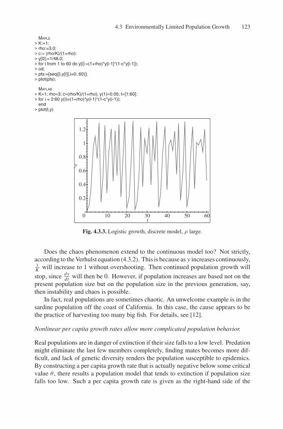
Recall that we encountered a similar recurrence relation, (2.5.11), in Section 2.5.From that discussion, we suspect that some values of ρ may lead to chaos. In fact,with K = 1 and ρ = 3, we get the population behavior shown in Figure 4.3.3.


MAPLE

> K:=1;> rho:=3.0;> c:= (rho/K)/(1+rho):> y[0]:=1/48.0;> for i from 1 to 60 do y[i]:=(1+rho)*y[i-1]*(1-c*y[i-1]);> od;> pts:=[seq([i,y[i]],i=0..60)];> plot(pts);

MATLAB

> K=1; rho=3; c=(rho/K)/(1+rho); y(1)=0.05; t=[1:60];> for i = 2:60 y(i)=(1+rho)*y(i-1)*(1-c*y(i-1));

end> plot(t,y)

0

0.2

0.4

0.6

0.8

1

1.2

y

10 20 30 40 50 60t

Fig. 4.3.3. Logistic growth, discrete model, ρ large.

Does the chaos phenomenon extend to the continuous model too? Not strictly,according to the Verhulst equation (4.3.2). This is because as y increases continuously,yK

will increase to 1 without overshooting. Then continued population growth will

stop, since dydt

will then be 0. However, if population increases are based not on thepresent population size but on the population size in the previous generation, say,then instability and chaos is possible.

In fact, real populations are sometimes chaotic. An unwelcome example is in thesardine population off the coast of California. In this case, the cause appears to bethe practice of harvesting too many big fish. For details, see [12].

Nonlinear per capita growth rates allow more complicated population behavior.

Real populations are in danger of extinction if their size falls to a low level. Predationmight eliminate the last few members completely, finding mates becomes more dif-ficult, and lack of genetic diversity renders the population susceptible to epidemics.By constructing a per capita growth rate that is actually negative below some criticalvalue θ , there results a population model that tends to extinction if population sizefalls too low. Such a per capita growth rate is given as the right-hand side of the


following modification of the logistic equation:

1

y

dy

dt= r

(y

θ− 1) (

1− y

K

), (4.3.11)

where 0 < θ < K . This form of the per capita growth rate is pictured in Figure 4.3.4using the specific parameters r = 1, θ = 1

5 , and K = 1. It is sometimes referred toas the predator pit.

We draw the graph in Figure 4.3.4 with these parameters:

MAPLE

> restart> r:=1; theta:=1/5; K:=1;> plot([y,r*(y/theta-1)*(1-y/K),y=0..1],-.2..1,-1..1);

MATLAB

> r=1; theta=0.2; K=1; y=0:0.05:1; f=r.*(y/theta - 1).*(1-y/K);> plot(y,f); hold on> xaxis = zeros(size(y));> plot(y,xaxis)

y ¢/y

y

–1

-0.5

0

0.5

1

–0.2 0 0.2 0.4 0.6 0.8 1

Fig. 4.3.4. The predator pit per capita growth rate function.

The stationary points of (4.3.11) are y = 0, y = θ , and y = K . Unlike before,now y = 0 is asymptotically stable; that is, if the starting value y0 of a solution isnear enough to 0, then the solution will tend to 0 as t increases. This follows becausethe sign of the right-hand side of (4.3.11) is negative for 0 < y < θ , causing dy

dt< 0.

Hence y will decrease. On the other hand, a solution starting with y0 > θ tends toK as t increases. This follows because when θ < y < K , the right-hand side of(4.3.11) is positive, so dy

dt> 0 also and hence y will increase even more. As before,

solutions starting above K decrease asymptotically to K .Some solutions to (4.3.11) are shown in Figure 4.3.5 with the following syntax:


0

0.5

1

1.5

y

0 1 2 3t

Fig. 4.3.5. Some solutions to the predator pit equation.

MAPLE

> r:=1; theta:=1/5; K:=1;> inits:={[0,.05],[0,.1],[0,0.3],[0,.5],[0,1],[0,0.7],[0,1.5]};> with(DEtools): DEplot(diff(y(t),t)=r*y(t)*(y(t)/theta-1)*(1-y(t)/K),y(t),t=0..3,inits, arrows=NONE,stepsize=0.1);

MATLAB

% Make up an m-file, fig434.m:% function yprime = fig434(t,y)% with r=1, theta=.2, and K=1.% r=1; theta=0.2; K=1;% yprime = y.*r.*(1-y./K).*(y/theta-1);

> tspan=[0 3];> [t05,y05]=ode23(’fig434’,tspan,.05);> [t1,y1]=ode23(’fig434’,tspan,.1);> [t3,y3]=ode23(’fig434’,tspan,.3);> [t5,y5]=ode23(’fig434’,tspan,.5);> [t7,y7]=ode23(’fig434’,tspan,.7);> [t15,y15]=ode23(’fig434’,tspan,1.5);> plot(t05,y05,t1,y1,t3,y3,t5,y5,t7,y7,t15,y15)

As our last illustration, we construct a population model that engenders littlepopulation growth for small populations, rapid growth for intermediate sized ones,and low growth again for large populations. This is achieved by the quadratic percapita growth rate and given as the right-hand side of the differential equation

1

y

dy

dt= ry

(1− y

K

). (4.3.12)

Exercises/Experiments

1. At the meeting of the Southeastern Section of the Mathematics Association ofAmerica, Terry Anderson presented a Maple program that determined a logisticfit for the U.S. population data. His fit is given by

U.S. population ≈ α

1+ βe−δt,


where α = 387.9802, β = 54.0812, and δ = 0.0270347. Here population ismeasured in millions and t = time since 1790. (Recall the population data ofExample 3.5.1.)(a) Show that the function given by the Anderson fit satisfies a logistic equation

of the formdy

dt= δy(t)

(1− y(t)

α

),

withy(0) = α

1+ β.

(b) Plot the graphs of the U.S. population data and this graph superimposed.Compare the exponential fits from Chapter 3.

(c) If population trends continue, what is the long-range fit for the U.S. popula-tion level?

MAPLE

> Anderfit:=t–>alpha/(1+beta*exp(-delta*t));> dsolve({diff(y(t),t)-delta*y(t)*(1-y(t)/alpha)=0, y(0)=alpha/(1+beta)},y(t));> alpha:=387.980205; beta:=54.0812024; delta:=0.02270347337;> J:=plot(Anderfit(t),t=0..200):> tt:=[seq(i*10,i=0..20)];> pop:=[3.929214, 5.308483, 7.239881, 9.638453, 12.866020, 17.069453, 23.191876,

31.433321, 39.818449, 50.155783, 62.947714, 75.994575, 91.972266, 105.710620,122.775046, 131.669275, 151.325798, 179.323175, 203.302031, 226.545805,248.709873];

> data:= [seq([tt[i],pop[i]],i=1..21)];> K:=plot(data,style=POINT):> plots[display]({J,K});> expfit:= t–>exp(0.02075384393*t+1.766257672);> L:=plot(expfit(t),t=0..200):> plots[display]({J,K,L});> plot(Anderfit(t-1790),t=1790..2150);

MATLAB

> tt=0:10:200;> pop=[3.929214, 5.308483, 7.239881, 9.638453, 12.866020, 17.069453, 23.191876,…

31.433321, 39.818449, 50.155783, 62.947714, 75.994575, 91.972266, 105.710620,…122.775046, 131.669275, 151.325798, 179.323175, 203.302031, 226.545805,…248.709873];

> plot(tt,pop,’x’); hold on;> alpha=387.980205; beta=54.0812024; delta=0.02270347337;> Anderfit=alpha./(1+beta*exp(-delta*tt));> plot(tt,Anderfit)

2. Using the method of (4.3.8), get a logistic fit for the U.S. population. Use thedata in Example3.5.1.

3. Suppose that the spruce budworm, in the absence of predation by birds, will growaccording to a simple logistic equation of the form

dB

dt= rB

(1− B

K

).

Budworms feed on the foliage of trees. The size of the carrying capacity, K , willtherefore depend on the amount of foliage on the trees; we take it to be constantfor this model.


(a) Draw graphs for how the population might grow if r were 0.48 and K were15. Use several initial values.

(b) Introduce predation by birds into this model in the following manner: Sup-pose that for small levels of worm population there is almost no predation,but for larger levels, birds are attracted to this food source. Allow for a limitto the number of worms that each bird can eat. A model for predation bybirds might have the form

P(B) = aB2

b2 + B2,

where a and b are positive (see [7]). Sketch the graph for level of predationof the budworms as a function of the size of the population. Take a and b

to be 2.

(c) A model for the budworm population size in the presence of predation couldbe modeled as

dB

dt= rB

(1− B

K

)− a

B2

b2 + B2.

To understand the delicacy of this model and the implications for the carethat needs to be taken in modeling, investigate graphs of solutions for thismodel with parameters r = 0.48, a = b = 2, and K = 15 or K = 17.

(d) Verify that in one case, there is a positive steady-state solution and in theother, the limit of the budworm population is zero.The significance of the graph with K = 17 is that the worm populationcan rise to a high level. With K = 15, only a low level for the size of thebudworms is possible. The birds will eat enough of the budworms to savethe trees!Here is the syntax for making this study with K = 15:

MAPLE

> K:= 15;> h:=(t,B)–>.48*B*(1-B/K)-2*Bˆ2/(4+Bˆ2);> plot(h(0,B),B=0..20);> inits:={[0,1], [0,2], [0,4], [0,5], [0,6], [0,8], [0,10], [0,12], [0,14], [0,16]};> with(DEtools);> DEplot(diff(y(t),t)=h(t,y(t)),y(t),t=0..30,inits,arrows=NONE,stepsize=0.1);

MATLAB

% make an m-file, exer43.m% function Bprime=exer43(t,B); r=.48; K=15; a=2; b=2; Bprime=r*B.*(1-B/K)-a*B.ˆ2./(bˆ2+B.ˆ2);

> K=15; a=2; b=2; r=.48;> B=0:.1:20; Bprime=exer43(0,B); plot(B,Bprime)> [t,y1]=ode23(’exer43’,[0 30],1);plot(t,y1)> hold on> [t,y2]=ode23(’exer43’,[0 30],2);plot(t,y2)> [t,y4]=ode23(’exer43’,[0 30],4);plot(t,y4)> [t,y5]=ode23(’exer43’,[0 30],5);plot(t,y5)> [t,y6]=ode23(’exer43’,[0 30],6);plot(t,y6)> [t,y8]=ode23(’exer43’,[0 30],8);plot(t,y8)> [t,y10]=ode23(’exer43’,[0 30],10);plot(t,y10)> [t,y12]=ode23(’exer43’,[0 30],12);plot(t,y12)> [t,y14]=ode23(’exer43’,[0 30],14);plot(t,y14)> [t,y16]=ode23(’exer43’,[0 30],16);plot(t,y16)


4. The following is a logistic adaptation of Code 3.5.1. Experiment with the pa-rameter r and observe the behavior of the population size. Is the size chaotic forsome values of r? It might be necessary to decrease delT (by increasing N to,say, 20) to get valid results.

MAPLE

> N:=10: delT:=1/N:#t is now linked to index i by t=-1+(i-1)*delT

> for i from 1 to N+1 do f[i]:=1:od:

> #work from t=0 in steps of delT> tfinal:=10: #end time tfinal, end index is n> n:=(tfinal+1)*N+1:> K:=3; r:=1.2;> for i from N+1 to n-1 do t:=-1+(i-1)*delT:

delY:=r*f[i-N]*(1-f[i-N]/K)*delT: #N back=delay of 1f[i+1]:=f[i]+delY: #Eulers method

> od;> pts:=[seq([i,f[i]],i=0..n)];> plot(pts);

MATLAB

% make an m-file, delayFcn0.m:% function y=delayFcn0(t)% y = 1;

> N=10; % steps per unit interval> delT=1/N; % so delta t=0.1

% t is now linked to index i by t=-1+(i-1)*delT% set initial values via delay fcn f0

> for i=1:N+1> t=-1+(i-1)*delT; f(i)=delayFcn0(t);> end

% work from t=0 in steps of delTtfinal=10; % end time tfinal, end index is n% solve tfinal=-1+(n-1)*delT for n

> n=(tfinal+1)*N+1;> K=3; r=1.2;> for i=N+1:n-1> t=-1+(i-1)*delT;> delY=r*f(i-N)*(1-f(i-N)/K)*delT; % N back=delay of 1> f(i+1)=f(i)+delY; % Eulers method> end> t=-1:delT:tfinal; plot(t,f);

4.4 A Brief Look at Multiple Species Systems

Without exception, biological populations interact with populations of other species.Indeed, the web of interactions is so pervasive that the entire field of Ecology isdevoted to it. Mathematically, the subject began about 70 years ago with a simple two-species, predator–prey differential equation model. The central premise of this Lotka–Volterra model is a mass action–interaction term. While community differentialequation models are difficult to solve exactly, they can nonetheless be analyzed byqualitative methods. One tool for this is to linearize the system of equations abouttheir stationary solution points and to determine the eigenvalues of the resultinginteraction, or community, matrix. The eigenvalues in turn predict the stability ofthe web. The Lotka–Volterra system has neutral stability at its nontrivial stationary

4.4 A Brief Look at Multiple Species Systems 129

point, which, like Malthus’s unbounded population growth, is a shortcoming thatindicates the need for a better model.

Interacting population models utilize a mass action–interaction term.

Alfred Lotka (1925) and, independently, Vito Volterra (1926) proposed a simplemodel for the population dynamics of two interacting species (see [8]). The centralassumption of the model is that the degree of interaction is proportional to the numbers,x and y, of each species and hence to their product, that is,

degree of interaction = (constant)xy.

The Lotka–Volterra system is less than satisfactory as a serious model because itentails neutral stability (see below). However, it does illustrate the basic principles ofmultispecies models and the techniques for their analysis. Further, like the Malthusianmodel, it serves as a point of departure for better models. The central assumptionstated above is also used as the interaction term between reactants in the descriptionof chemical reactions. In that context it is called the mass action principle. Theprinciple implies that encounters occur more frequently in direct proportion to theirconcentrations.

The original Lotka–Volterra equations are

dx

dt= rx − axy,

dy

dt= −my + bxy,

(4.4.1)

where the positive constants r , m, a, and b are parameters. The model was meant totreat predator–prey interactions. In this, x denotes the population size of the prey, andy the same for the predators. In the absence of predators, the equation for the preyreduces to dx

dt= rx. Hence the prey population increases exponentially with rate r

in this case; see Section 3.5. Similarly, in the absence of prey, the predator equationbecomes dy

dt= −my, dictating an exponential decline with rate m.

The sign of the interaction term for the prey, −a, is negative, indicating thatinteraction is detrimental to them. The parameter a measures the average degree ofthe effect of one predator in depressing the per capita growth rate of the prey. Thus a

is likely to be large in a model for butterflies and birds but much smaller in a modelfor caribou and wolves. In contrast, the sign of the interaction term for the predators,+b, is positive, indicating that they are benefited by the interaction. As above, themagnitude of b is indicative of the average effect of one prey on the per capita predatorgrowth rate.

Besides describing predator–prey dynamics, the Lotka–Volterra system describesto a host–parasite interaction as well. Furthermore, by changing the signs of theinteraction terms, or allowing them to be zero, the same basic system applies toother kinds of biological interactions as discussed in Section 4.1, such as mutualism,competition, commensalism, and amensalism.


Mathematically, the Lotka–Volterra system is not easily solved. Nevertheless,solutions may be numerically approximated and qualitatively described. Since thesystem has two dependent variables, a solution consists of a pair of functions x(t) andy(t) whose derivatives satisfy (4.4.1). Figure 4.4.1 is the plot of the solution to theseequations with r = a = m = b = 1 and initial values x(0) = 1.5 and y(0) = 0.5.The figure is drawn with the following syntax:

MAPLE

> predprey:=diff(x(t),t)=r*x(t)-a*x(t)*y(t), diff(y(t),t)=-m*y(t)+b*x(t)*y(t);> r:=1; a:=1; m:=1; b:=1;> sol:=dsolve({predprey,x(0)=3/2,y(0)=1/2}, {x(t),y(t)},type=numeric, output=listprocedure);> xsol:=subs(sol,x(t)); ysol:=subs(sol,y(t));> plot([xsol,ysol],0..10,-1..3);

MATLAB

% make an m-file named predPrey44.m with:% function Yprime=predPrey44(t,x)% r=1; a=1; m=1; b=1;% Yprime=[r∗x(1)-a*x(1).*x(2); -m*x(2)+b*x(1).*x(2)];

> [t,Y]=ode23(’predPrey44’,[0 10],[1.5;0.5]); % ; for column vector> plot(t,Y) % both curves as the columns of Y vs. t

t

x (t)

y (t)

–1

0

1

2

3

–2 0 2 4 6 8 10

Fig. 4.4.1. Graphs of x(t) and of y(t), solutions for (4.4.1).

Notice that the prey curve leads the predator curve.5 We discuss this next.Although there are three variables in a Lotka–Volterra system, t is easily elimi-

nated by dividing dydt

by dxdt

; thus

5 In Section 4.1, we have discussed a number of biological reasons why in a real situation,this model is inadequate.


MAPLE

> with(plots): with(DEtools):> inits:={[0,3/2,1/2],[0,4/5,3/2]};> phaseportrait({predprey},[x,y],t=0..10,inits,stepsize=.1);

MATLAB

> x=Y(:,1); y=Y(:,2); plot(x,y)

A

B

C

D

0.5

1

1.5

2

y

0.5 1 1.5 2x

Fig. 4.4.2. A plot of two solutions of (4.4.1) in the (x, y)-plane.

dy

dx= −my + bxy

rx − axy.

This equation does not contain t and can be solved exactly as an implicit relationbetween x and y:6

MAPLE

> dsolve(diff(y(x),x)=(-y(x)+x*y(x))/(x-x∗y(x)),y(x),implicit);

− ln(y(x))+ y(x)− ln(x)+ x = C.

This solution gives rise to a system of closed curves in the (x, y)-plane called thephase plane of the system. These same curves, or phase portraits, can be generatedfrom a solution pair x(t) and y(t) as above by treating t as a parameter. In Figure 4.4.2,we show the phase portrait of the solution pictured in Figure 4.4.1.

Let us now trace this phase portrait. Start at the bottom of the curve, region A,with only a small number of prey and predators. With few predators, the populationsize of the prey grows almost exponentially. But as the prey size becomes large, theinteraction term for the predators, bxy, becomes large and their numbers y begin togrow. Eventually, the product ay first equals and then exceeds r , in the first equationof (4.4.1), at which time the population size of the prey must decrease. This takes usto region B in the figure.

6 Implicit means that neither variable x nor y is solved for in terms of the other.


However, the number of prey is still large, so predator size y continues to grow,forcing prey size x to continue declining. This is the upward and leftward sectionof the portrait. Eventually, the product bx first equals and then falls below m in thesecond equation of (4.4.1), whereupon the predator size now begins to decrease. Thisis point C in the figure.

At first, the predator size is still at a high level, so the prey size will continueto decrease until it reaches its smallest value. But with few prey around, predatornumbers y rapidly decrease until finally the product ay falls below r . Then the preysize starts to increase again. This is region D in the figure. But the prey size is still ata low level, so the predator numbers continue to decrease, bringing us back to regionA and completing one cycle.

Thus the phase portrait is traversed counterclockwise, and as we have seen in theabove narration, the predator population cycle qualitatively follows that of the preypopulation cycle but lags behind it.

Of course the populations won’t change at all if the derivatives dxdt

and dydt

areboth zero in the Lotka–Volterra equations (4.4.1). Setting them to zero and solvingthe resulting algebraic system locates the stationary points,

0 = x · (r − ay),

0 = y · (−m+ bx).

Thus if x = mb

and y = ra

, the populations remain fixed. Of course, x = y = 0 isalso a stationary point.

Stability determinations are made from an eigenanalysis of the community matrix.

Consider the stationary point (0, 0). What if the system starts close to this point,that is, y0 and x0 are both very nearly 0? We assume that these values are so smallthat the quadratic terms in (4.4.1) are negligible, and we discard them. This is calledlinearizing the system about the stationary point. Then the equations become

dx

dt= rx,

dy

dt= −my.

(4.4.2)

Hence x will increase and y will further decrease (but not to zero) and a phase portraitwill be initiated as discussed above. The system will not, however, return to (0, 0).Therefore, this stationary point is unstable.

We can come to the same conclusion by rewriting the system (4.4.2) in matrix formand examining the eigenvalues of the matrix on the right-hand side. This matrix is[

r 00 −m

], (4.4.3)

and its eigenvalues are λ1 = r and λ2 = −m. Since one of these is real and positive,the conclusion is that the stationary point (0, 0) is unstable.


Now consider the stationary point x = mb

and y = ra

and linearize about it asfollows. Let ξ = x − m

band η = y − r

a. In these new variables, the first equation of

the system (4.4.1) becomes

dξ

dt= r

(ξ + m

b

)− a

(ξ + m

b

) (η + r

a

)= −am

bη − aξη.

Again discard the quadratic term; this yields

dξ

dt= −am

bη.

The second equation of the system becomes

dη

t= −m

(η + r

a

)+ b

(ξ + m

b

) (η + r

a

),

dη

dt= br

aξ + bξη.

And discarding the quadratic term gives

dη

dt= br

aξ.

Thus the equations in (4.4.1) become

dξ

dt= −am

bη,

dη

dt= br

aξ.

(4.4.4)

The right-hand side of (4.4.4) can be written in matrix form:[0 − am

bbra

0

] [ξ

η

]. (4.4.5)

This time the eigenvalues of the matrix are imaginary, λ = ±i√

mr . This impliesthat the stationary point is neutrally stable.

Determining the stability at stationary points is an important problem. Linearizingabout these points is a common tool for studying this stability, and has been formalizedinto a computational procedure. In the exercises, we give more applications thatutilize the above analysis and that use a computer algebra system. Also, we give anexample in which the procedure incorrectly predicts the behavior at a stationary point.The text by Steven H. Strogatz [9] explains conditions under which the procedure isguaranteed to work.

To illustrate a computational procedure for this predator–prey model, first createthe vector function V :


MAPLE

> restart:> with(LinearAlgebra):with(VectorCalculus):> V:=Vector([r∗x-a∗x∗y,-m∗y+b∗x∗y]);

MATLAB

% We must compute derivates numerically% make an m-file predPrey44.m with:% function Yprime=predPrey44(t,x);% r=1; a=1; m=1; b=1;% Yprime=[r*x(1)-a*x(1).*x(2); -m*x(2)+b*x(1).*x(2)];

Find the critical points of (4.4.1) by asking where this vector-valued function is zero(symbolically):

MAPLE

> solve({V[1]=0,V[2]=0}, {x,y});

This investigation provides the solutions {0, 0} and {mb, r

a}, as we stated above. We

now make the linearization of V about {0, 0} and about {mb, r

a}:

MAPLE

> Jacobian(V,[x,y]);> subs({x=0,y=0},%);> subs({x=m/b,y=r/a},%%);

MATLAB

% eps is matlab’s smallest value; by divided difference% find the derivatives numerically; first at (0,0)

> M1=(predPrey44(0,[eps 0]) - predPrey44(0,[0 0]))/eps;% this is the first column of the Jacobian at x=y=0, i.e., derivatives with respect to x

> M2=(predPrey44(0,[0 eps]) - predPrey44(0,[0 0]))/eps;% the derivatives with respect to y

> M=[M1 M2]; % the Jacobian% calculate its eigenvalues

> eig(M) % get 1 and -1, +1 means unstable at (0,0)

Note that in matrix form,( dxdtdydt

)=(

r 00 −m

)(x − 0

y − 0

)+(−a

b

)(x − 0)(y − 0)

for linearization about (0, 0) and

( dxdtdydt

)=(

0 − amb

bra

0

)(x − m

b

y − ra

)+(−a

b

)(x − m

b

) (y − r

a

)for linearization about (m

b, r

a). Finally, we compute the eigenvalues for the lineariza-

tion about each of the critical points:MAPLE

> Eigenvalues(%%); Eigenvalues(%%);

MATLAB

% now linearize at x=m/b=1, y=r/a=1> M1=(predPrey44(0,[1+eps 1])-predPrey44(0,[1 1]))/eps;> M2=(predPrey44(0,[1 1+eps])-predPrey44(0,[1 1]))/eps;> M=[M1 M2];> eig(M) % get +/-I (I=sqrt(-1)), so neutrally stable

The result is the same as that from (4.4.5).


Exercises/Experiments

1. The following competition model is provided in [9]. Imagine rabbits and sheepcompeting for the same limited amount of grass. Assume a logistic growth forthe two populations, that rabbits reproduce rapidly, and that the sheep will crowdout the rabbits. Assume that these conflicts occur at a rate proportional to the sizeof each population. Further, assume that the conflicts reduce the growth rate foreach species, but make the effect more severe for the rabbits by increasing thecoefficient for that term. A model that incorporates these assumptions is

dx

dt= x(3− x − 2y),

dy

dt= y(2− x − y),

where x(t) is the rabbit population and y is the sheep population. (Of course, thecoefficients are not realistic but are chosen to illustrate the possibilities.) Findfour stationary points and investigate the stability of each. Show that one of thetwo populations is driven to extinction.

2. Imagine a three-species predator–prey problem that we identify with grass, sheep,and wolves. The grass grows according to a logistic equation in the absence ofsheep. The sheep eat the grass and the wolves eat the sheep. (See McLaren[10] for a three-species population under observation.) We model this with theequations that follow. Here x represents the wolf population, y represents thesheep population, and z represents the area in grass:

dx

dt= −x + xy,

dy

dz= −y + 2yz− xy,

dz

dt= 2z− z2 − yz.

What would be the steady state of grass with no sheep or wolves present? Whatwould be the steady state of sheep and grass with no wolves present? What isthe revised steady state with wolves present? Does the introduction of wolvesbenefit the grass? This study can be done as follows:

MAPLE

> restart:> rsx:=-x(t)+x(t)*y(t);> rsy:=-y(t)+2*y(t)*z(t)-x(t)*y(t);> rsz:= 2*z(t)-z(t)ˆ2-y(t)*z(t);

MATLAB

% make an m-file, exer442.m% function Yprime=exer442(t,Y); % Y(1)=x, Y(2)=y, Y(3)=z;% Yprime=[-Y(1)+Y(1).*Y(2); -Y(2)+2*Y(2).*Y(3)-Y(1).*Y(2); 2*Y(3)-Y(3).*Y(3)-Y(2).*Y(3)];

For just grass:


MAPLE

> sol:=dsolve({diff(x(t),t)=rsx,diff(y(t),t)=rsy,diff(z(t),t)=rsz,x(0)=0,y(0)=0,z(0)=1.5},{x(t),y(t),z(t)},type=numeric,output=listprocedure);

> zsol:=subs(sol,z(t)); zsol(1);> plot(zsol,0..20,color=green);

MATLAB

% grass> [t,Y]=ode23(’exer442’,[0 200],[0; 0; 1.5]);> plot(t,Y(:,3))

For grass and sheep:MAPLE

> sol:=dsolve({diff(x(t),t)=rsx,diff(y(t),t)=rsy,diff(z(t),t)=rsz,x(0)=0,y(0)=.5,z(0)=1.5},{x(t),y(t),z(t)},type=numeric,output=listprocedure);

> ysol:=subs(sol,y(t));zsol:=subs(sol,z(t));> plot([ysol,zsol],0..20,color=[green,black]);

MATLAB

% grass and sheep> [t,Y]=ode23(’exer442’,[0 200],[0; .5; 1.5]);> plot(t,Y)

For grass, sheep, and wolves:MAPLE

> sol:=dsolve({diff(x(t),t)=rsx,diff(y(t),t)=rsy,diff(z(t),t)=rsz,x(0)=.2,y(0)=.5,z(0)=1.5},{x(t),y(t),z(t)},type=numeric,output=listprocedure);

> xsol:=subs(sol,x(t));> ysol:=subs(sol,y(t));> zsol:=subs(sol,z(t));> plot([xsol,ysol,zsol],0..20,color=[green,black,red]);

MATLAB

% all three> [t,Y]=ode23(’exer442’,[0 200],[.2; .5; 1.5]);> plot(t,Y(:,3),’g’) % grass behavior> hold on> plot(t,Y(:,2),’b’) % sheep behavior> plot(t,Y(:,1),’r’) % wolf behavior

3. J. M. A. Danby [11] has a collection of interesting population models in hisdelightful text. The following predator–prey model with child care is included.Suppose that the prey x(t) is divided into two classes, x1(t) and x2(t), of youngand adults. Suppose that the young are protected from predators y(t). Assumethat the young increase in proportion to the number of adults and decrease dueto death or to moving into the adult class. Then

dx1

dt= ax2 − bx1 − cx1.

The number of adults is increased by the young growing up and decreased bynatural death and predation, so that we model

dx2

dt= bx1 − dx2 − ex2y.

Finally, for the predators, we take

dy

dt= −fy + gx2y.


Investigate the structure for the solutions of this model. Parameters that mightbe used are

a = 2, b = c = d = 1

2, and e = f = g = 1.

4. Show that the linearization of the system

dx

dt= −y + ax(x2 + y2),

dy

dt= x + ay(x2 + y2)

predicts that the origin is a center for all values of a, whereas, in fact, the originis a stable spiral if a < 0 and an unstable spiral if a > 0. Draw phase portraitsfor a = 1 and a = −1.

5. Suppose there is a small group of individuals who are infected with a contagiousdisease and who have come into a larger population. If the population is dividedinto three groups—the susceptible, the infected, and the recovered—we havewhat is known as a classical S–I–R problem. (We take up such problems againin Section 11.4.) The susceptible class consists of those who are not infected,but who are capable of catching the disease and becoming infected. The infectedclass consists of the individuals who are capable of transmitting the disease toothers. The recovered class consists of those who have had the disease, but areno longer infectious.A system of equations that is used to model such a situation is often described asfollows:

dS

dt= −rS(t)I (t),

dI

dt= rS(t)I (t)− aI (t),

dR

dt= aI (t)

for positive constants r and a. The proportionality constant r is called the infec-tion rate and the proportionality constant a is called the removal rate.

(a) Rewrite this model as a matrix model and recognize that the problem formsa closed compartment model. Conclude that the total population remainsconstant.

(b) Draw graphs for solutions. Observe that the susceptible class decreases insize and that the infected size increases in size and later decreases.

MAPLE

> r:=1; a:=1;> sol:=dsolve({diff(SU(t),t)=-r*SU(t)*IN(t),diff(IN(t),t)=r*SU(t)*IN(t)-a*IN(t),diff(R(t),t)=a*IN(t),

SU(0)=2.8,IN(0)=0.2,R(0)=0},{SU(t),IN(t),R(t)},type=numeric,output=listprocedure):> f:=subs(sol,SU(t)): g:=subs(sol,IN(t)): h:=subs(sol,R(t));> plot({f,g,h},0..20,color=[green,red,black]);


MATLAB

% contents of the m-file exer445a.m:% function SIRprime=exer445a(t,SIR); % S=SIR(1), I=SIR(2), R=SIR(3);% r=1; a=1;% SIRprime=[-r*SIR(1).*SIR(2); r*SIR(1).*SIR(2)-a*SIR(2);a*SIR(2)];

> r=1; a=1;> [t,SIR]=ode45(’exer445a’,[0 20], [2.8; .2; 0]);> plot(t,SIR)

(c) Suppose now that the recovered do not receive permanent immunity. Rather,we suppose that after a delay of one unit of time, those who have recoveredlose immunity and move into the susceptible class. The system of equationschanges to the following:

dS

dt= −rS(t)I (t)+ R(t − 1),

dI

dt= rS(t)I (t)− aI (t),

dR

dt= aI (t)− R(t − 1).

Draw graphs for solutions to this system. Observe the possibility of oscil-lating solutions. How do you explain these oscillations from the perspectiveof an epidemiologist? (Note: The following has a long run time.)

MAPLE

> restart:with(plots):> N:=5;> f[0]:=t–>2.8; g[0]:=t–>0.2*exp(-tˆ2); h[0]:=t–>0;> P[0]:=plot([[t,f[0](t),t=-1..0],[t,g[0](t),t=-1..0],[t,h[0](t),t=-1..0]],color=[green,red,black]):> for n from 1 to N do> sol:=dsolve({diff(SU(t),t)=-SU(t)*IN(t)+h[n-1](t-1),diff(IN(t),t)=SU(t)*IN(t)-IN(t),

diff(R(t),t)=IN(t)-h[n-1](t-1),SU(n-1)=f[n-1](n-1),IN(n-1)=g[n-1](n-1),R(n-1)=h[n-1](n-1)},{SU(t),IN(t),R(t)},numeric,output=listprocedure,known=h[n-1]):

> f[n]:=subs(sol,SU(t)); g[n]:=subs(sol,IN(t));> h[n]:=subs(sol,R(t)):> P[n]:=plot([[t,f[n](t),t=n-1..n],[t,g[n](t),t=n-1..n],[t,h[n](t),t=n-1..n]],color=[green,red,black]):> od:> n:=’n’;> J:=plot([t,1,t=0..N],color=blue):> display([J,seq(P[n],n=0..N)]);> for n from 1 to N do> Q[n]:=spacecurve([f[n](t),g[n](t),h[n](t)],t=n-1..n,axes=normal,color=black):> od:> PP:=pointplot3d([1,1,1],axes=normal,symbol=diamond,color=green):> display([PP,seq(Q[n],n=1..N)]);

MATLAB

> N=100; % number steps per unit interval> delT=1/N; % so delta t=0.01

% t is now linked to index i by t=-1+(i-1)*delT, where i=1,2,...,nFinal% and the final index nFinal is given by solving tFinal = -1+(nFinal-1)*delT.

> tFinal=5; nFinal=(tFinal+1)*N+1;% set up the initial values of R on -1 to 0

> for i=1:N> R(i)=0; S(i)=0; I(i)=0;> end

% work from t=0 in steps of delT> S(N+1)=2.8; I(N+1)=0.2; R(N+1)=0;> for i=N+1:nFinal-1> delY=delT*[-r*S(i)*I(i)+R(i-N); r*S(i)*I(i)-a*I(i); a*I(i)-R(i-N)]; S(i+1)=S(i)+delY(1);…

I(i+1)=I(i)+delY(2); R(i+1) = R(i)+delY(3);

References and Suggested Further Reading 139

> end% graph it

> t=-1:delT:tFinal;> plot(t,S,t,I,t,R) % S blue, I green, R red

Questions for Thought and Discussion

1. Name and discuss four factors that affect the carrying capacity of an environmentfor a given species.

2. Draw and explain the shape of survivorship and population growth curves for anr-strategist.

3. Draw and explain the shape of survivorship and population growth curves for aK-strategist.

4. Define carrying capacity and environmental resistance.

5. Discuss the concept of parental investment and its role in r- and K-strategies.

References and Suggested Further Reading

[1] Environmental resistance:W. T. Keeton and J. L. Gould, Biological Science, 5th ed., Norton, New York, 1993.

[2] Partitioning of resources:J. L. Harper, Population Biology of Plants, Academic Press, New York, 1977.

[3] Population ecology:R. Brewer, The Science of Ecology, 2nd ed., Saunders College Publishing, Fort Worth,TX, 1988.

[4] Ecology and public issues:B. Commoner, The Closing Circle: Nature, Man, and Technology, Knopf, New York,1971.

[5] Natural population control:H. N. Southern, The natural control of a population of tawny owls (Strix aluco), J. Zool.London, 162 (1970), 197–285.

[6] A doomsday model:D. A. Smith; Human population growth: Stability or explosion, Math. Magazine, 50-4(1977) 186–197.

[7] Budworm, balsalm fir, and birds:D. Ludwig, D. D. Jones, and C. S. Holling, Qualitative analysis of insect outbreak systems:The spruce budworm and forests, J. Animal Ecol., 47 (1978), 315–332.

[8] Predator or prey:J. D. Murray, Predator–prey models: Lotka–Volterra systems, in J. D. Murray, Mathe-matical Biology, Springer-Verlag, Berlin, 1990, Section 3.1.

[9] Linearization:S. H. Strogatz, Nonlinear Dynamics and Chaos, with Applications to Physics, Biology,Chemistry, and Engineering, Addison–Wesley, New York, 1994.

[10] A matter of wolves:B. E. McLaren and R. O. Peterson, Wolves, moose, and tree rings on Isle Royale, Science,266 (1994), 1555–1558.


[11] Predator–prey with child care, cannibalism, and other models:J. M. A. Danby, Computing Applications to Differential Equations, Reston PublishingCompany, Reston, VA, 1985.

[12] Chaos in biological populations:P. Raeburn, Chaos and the catch of the day, Sci. Amer., 300-2 (2009), 76–78.

4 Interactions Between Organisms and Their Environment

Documents

Transcript of 4 Interactions Between Organisms and Their Environment