3D visualization to assist iterative object definition from medical images

Computerized Medical Imaging and Graphics 30 (2006) 217–230

3D visualization to assist iterative object definitionfrom medical images

Romaric Audigier a1, Roberto Lotufo a, Alexandre Falcao b,∗a School of Electrical and Computer Engineering, State University of Campinas (UNICAMP) C.P. 6101, 13083-852 Campinas (SP), Brazilb Institute of Computing, State University of Campinas (UNICAMP) Av. Albert Einstein, 1251, C.P. 6176, 13084-971 Campinas (SP), Brazil

Abstract

In medical imaging, many applications require visualization and/or analysis of three-dimensional (3D) objects (e.g. organs). At same time,object definition often requires considerable user assistance. In this process, objects are usually defined in an iterative way and their visualizationduring the process is very important to guide the user’s actions for the next iteration. The usual procedure provides slice visualization during objectdefinition (segmentation) and 3D visualization afterward. In this paper, we propose and evaluate efficient methods to provide 3D visualizationduring iterative object definition. The methods combine the differential image foresting transform for segmentation with voxel splatting/ray castingf©

P

Ki

1

ipiisitdnfsi

0d

or visualization.2006 Elsevier Ltd. All rights reserved.

ACS: 87.57.Ra; 42.30.-d; 07.05.Rm; 02.10.Ox

eywords: 3D visualization; Interactive image segmentation; Watershed transform; Image foresting transform; Voxel splatting; Raycasting; Rendering of medicalmages

. Introduction

Computerized tomography (CT), magnetic resonance imag-ng (MRI) and other multidimensional imaging modalities haveromoted the practice of medicine in many different ways. Whenmages are acquired for a region of the human body (scene), theres usually an object system under study, which may be simply aet of organs within that scene. The purpose of image acquisitions mostly to fulfill some combination of the following objectives:he diagnosis of a disease, understanding the natural course of aisease, understanding the function of the object system, plan-ing a treatment for a disease, studying the effects of a treatmentor a disease and medical education. The precise spatial exten-ion (image segmentation) of the objects in the scene is crucialn many of these applications.

∗ Corresponding author. Tel.: +55 19 3788 5881; fax: +55 19 3788 5847.1 R. Audigier was funded by CAPES.

E-mail address: [email protected] (A. Falcao).URL: http://www.ic.unicamp.br/∼afalcao.

Image segmentation usually requires considerable user as-sistance. In this process, the objects are defined in an iterativeway and their visualization during the process is very importantto guide the user’s actions for the next iteration. The usual pro-cedure provides slice visualization (axial, coronal and sagittalviews) during object definition and three-dimensional (3D) vi-sualization afterward. While slice visualization may be justifiedby its interactive response time during segmentation, it providesa limited idea of the 3D shape and form of the objects—which isimportant for precise object definition. Therefore, our aim hereis to investigate solutions that obtain interactive times for objectdefinition with 3D visualization (i.e. a total time less than 5 s for3D segmentation and visualization. In the literature, for exam-ple, it seems reasonable to obtain 1 or 2 s for visualization only[1]).

The efforts to speed up 3D visualization have involved staticobject representations based on geometric primitives (e.g. tri-angles, voxels, voxel faces [2,3]), specialized hardware [4,5]and algorithms that trade off image quality for speed [6,7]. Inmost cases, complete object definition is required as a sepa-rated and prior step for 3D visualization. These techniques arenot applied to the present work, because we are interested in

895-6111/$ – see front matter © 2006 Elsevier Ltd. All rights reserved.oi:10.1016/j.compmedimag.2006.05.003

mailto:[email protected]

dx.doi.org/10.1016/j.compmedimag.2006.05.003

218 R. Audigier et al. / Computerized Medical Imaging and Graphics 30 (2006) 217–230

3D visualization of a dynamic structure system defined by it-erative object definition. The immediacy of response and inter-actability in 3D visualization have also called for methods thatavoid image segmentation and examine the scene as a semi-transparent volume [8–10]. An attempt is made in these meth-ods to portray the objects by appropriately assigning opacities tothe voxels. Unfortunately, opacity assignment is a difficult taskin many situations (e.g. bones in MRI) and object definition isstill required in several applications (e.g. quantitative analysis[11,12]).

More recently, the speed of the personal computers and ad-vances in image segmentation have allowed 3D visualizationduring object definition at interactive speeds [13]. The methodis based on the image foresting transform (IFT)—a general toolfor the design, implementation and evaluation of image process-ing operators based on connectivity [14]. In the IFT, a scene isinterpreted as a graph whose nodes are the voxels in the sceneand whose arcs are defined by an adjacency relation betweenvoxels. For a given set of seed voxels and suitable path-costfunction, the IFT computes (in linear time) a minimum-costpath forest in the graph whose roots are drawn from the seedset. That is, each rooted tree consists of voxels more stronglyconnected to its root than to any other seed. By selecting a seedset for each object (including background) and assigning a dis-tinct label per object, an object is defined by optimum path treesrooted at seeds with a same label. In ref. [13], the user canaeifgptia[

Divs1wfiiat

rtnSaopmt

2. Notation and definitions

Let I be the volumetric image dataset obtained from somemedical imaging modality (e.g. MRI, CT). We call I a scene,where each voxel t ∈ I has a value v(t) assigned to it.

An adjacency relation N is a binary irreflexive relation be-tween voxels of I (e.g. 6- and 26-connected relations in 3D).We use t ∈ N(s) to indicate that a voxel t is adjacent to avoxel s.

For a given scene I and adjacency relation N, the scene canbe interpreted as a graph whose nodes are the voxels in I andwhose arcs (s, t) ∈ N are defined between adjacent voxels. Inthis context, a path is a sequence of adjacent voxels. A pathwith terminal node t is denoted by πt . The path πt is trivial,when it consists of a single voxel 〈t〉. Otherwise, it can be de-fined by a path resulting from the concatenation πs · 〈s, t〉 of itslongest prefix πs with terminus s and the last arc (s, t), wheret ∈ N(s).

A predecessor map is a function P that assigns to each voxelt ∈ I either some other voxel s ∈ I or a distinctive marker nil notin I— in which case t is said to be a root of the map. A spanningforest is a predecessor map which contains no cycles— in otherwords, one which takes every voxel to nil in a finite number ofiterations. For any voxel t ∈ I, a spanning forest P defines a pathP∗(t) = πt as 〈t〉 if P(t) = nil, or recursively as P∗(s) · 〈s, t〉 ifP(t) = s �= nil.

f

efi

i

3

f[fdostf

wfotii

dd seeds and/or remove trees of the forest by selecting vox-ls in the scene, and the optimum path forest can be updatedn a differential way. Therefore, instead of computing one IFTrom the beginning for each iteration, the differential IFT al-orithm (DIFT) updates the segmentation results in time pro-ortional to the number of voxels in the modified regions ofhe scene. After each iteration of the DIFT, the algorithm vis-ts and projects all object voxels onto a viewing plane usingvoxel splatting technique [15–17] and the z-buffer algorithm

18].In this paper, we present two other ways of combining the

IFT algorithm with rendering techniques. The first algorithms a variant of the DIFT, which maintains a list of object borderoxels for speeding up voxel splatting after each iteration. Theecond approach uses ray casting [18] and voxel splatting [15–7] for situations where the viewing direction remains the same,hile the object changes between consecutive iterations. Wenally evaluate the DIFT-based methods with various medical

mage datasets and synthetic scenes, using the usual procedures base line—where a complete object definition is obtained withhe IFT algorithm before 3D visualization.

A first version of this work was published in ref. [19]. We haveevised the entire text, included more examples and improvedhe explanations about the methods. Section 2 introduces theotation and main definitions used in this paper. We present inection 3 the interactive segmentation methods using the IFTnd DIFT algorithms. The methods for 3D visualization duringbject definition are discussed in Section 4. This section alsoresents the algorithms of the two new approaches. The experi-ents and results are described in Section 5 and Section 6 states

he conclusions of this work.

A path-cost function f assigns to each path π a path cost(π), in some totally ordered set of cost values, whose maximumlement is denoted by+∞. A path π is optimum if f (π) ≤ f (τ)or any other path τ with the same terminus of π, irrespective ofts starting point.

An optimum-path forest is a spanning forest P such that P∗(t)s optimum for every voxel t ∈ I.

. Interactive IFT-based segmentation

The image foresting transform takes a scene I, a path-costunction f (which satisfies some conditions established in ref.14]) and an adjacency relation N; and returns an optimum-pathorest P. In order to define objects using the IFT, we assign aistinct label to each object and select at least one seed voxel perbject (including background). The path-cost function should beuch that voxels of a given object are more strongly connectedo its internal seeds than to any other. A suitable example is theunction fmax below:

fmax(〈t〉) ={

0, if, t ∈ S,

∞, otherwise.

fmax(π · 〈s, t〉) = max{fmax(π), δ(s, t)},(1)

here S is the set of seed voxels and δ(s, t) is a dissimilarityunction between s and t, usually computed based on propertiesf the input scene I. Ideally, function δ(s, t) must be higher onhe object boundaries and lower inside the objects. For example,n the watershed transform [20], δ(s, t) is equal to some gradientntensity at voxel t. After that, the IFT outputs an optimum-path

R. Audigier et al. / Computerized Medical Imaging and Graphics 30 (2006) 217–230 219

forest where each object is represented by a set of trees rootedat seeds with the same label.

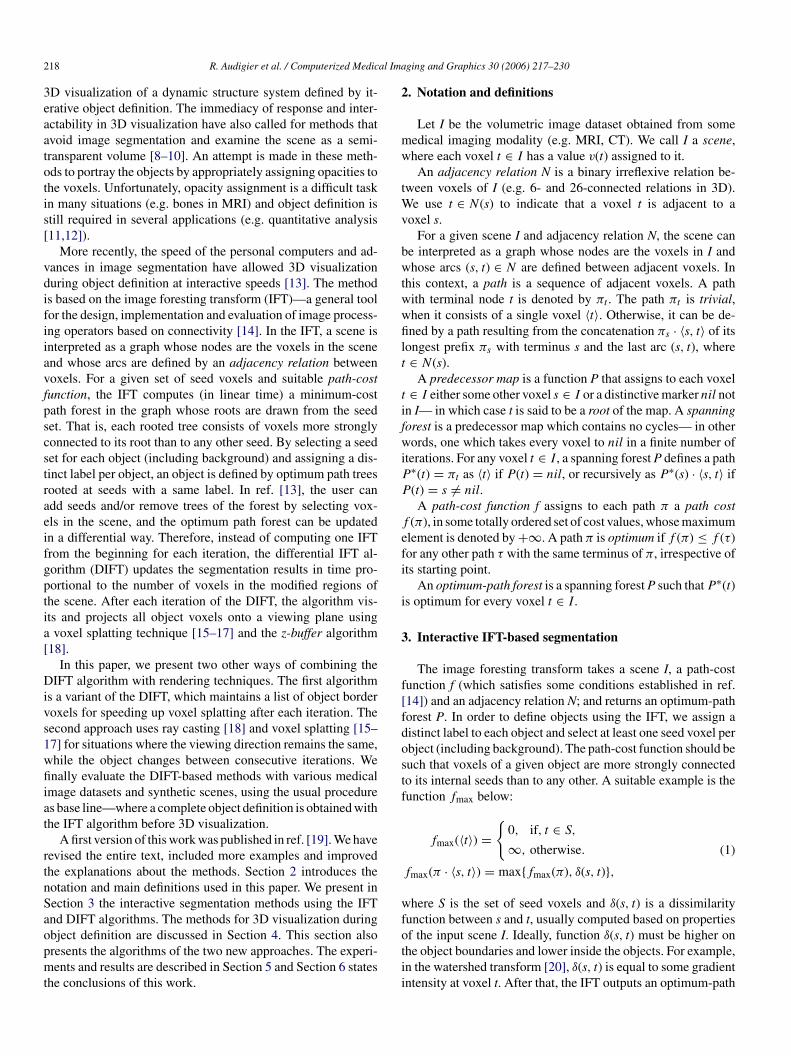
The IFT algorithm is essentially Dijkstra’s algorithm [21], ex-tended for multiple sources and a more general path-cost func-tion (see Pseudocode 1). It computes three attributes for eachvoxel t ∈ I: its predecessor P[t] in the optimum path, the costC[t] of that path and the corresponding root R[t]. After cost, rootand predecessor initializations (l. 1–2), a loop for emptying thepriority queue Q starts (l. 3–10). This ordered queue has beenfilled firstly with seed voxels (l. 2). The voxel s of highest prior-ity, i.e. lowest cost, is removed from Q (l. 4) with its definitiveattributes (cost C[s], root R[s] and predecessor P[s]). This indi-cates that the optimum path πs from some seed in S to the voxels has already be found. For each voxel t adjacent to s, such thatt has not been definitively processed, the cost c of a candidatepath πs · 〈s, t〉 with terminus t is evaluated (l. 5–6). If c is lowerthan the already assigned cost C[t] (l. 7), then the path πs · 〈s, t〉is considered better than the current path that reaches t and thethree attributes of t are updated (l. 8). If t has never been visited(i.e. t is not in Q), it is inserted in Q with cost c. Otherwise, only

its position in Q is updated (l. 9–10). Note that, for N definedby 6- or 26-adjacency, the priority queue Q can be implementedsuch that the IFT algorithm will run in time proportional to thenumber of voxels [14].

3.1. Differential IFT

Very often the user needs to correct segmentation by addingnew seeds and/or removing roots (trees), forming a sequence ofIFTs. Instead of computing one IFT for each instance of seedset, the DIFT algorithm [13] updates the segmentation results ina differential way. That is, when a voxel is added to the seed set,it may define a new optimum-path tree by invading the influencezones of other roots (i.e. the regions of voxels assigned to otherroots in the previous iteration of the DIFT). When a voxel isremoved from the seed set, the corresponding optimum-pathtree is removed from the forest and its voxels become availablefor a new dispute among the remaining roots (see Pseudocode2).


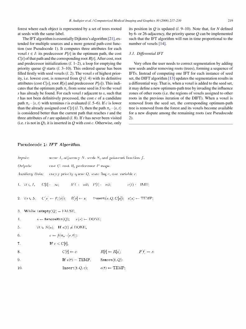
Fig. 1. Non-differential segmentation with 3D visualization by object projection.

In addition to the standard input parameters, the results ofthe previous iteration (costs C, roots R and predecessors P) areused as input together with a set S of new seeds and a set Eof eliminators (i.e. voxels that mark trees for removal). In eachDIFT iteration, voxels are initialized with a ‘not processed’ sta-tus (e(t)← INIT, l. 1). When a voxel is in the priority queue, itassumes an ‘in processing’ status (e(t)← TEMP, l. 3 and 11).And when it finally leaves the queue with definitive attributes,it gets a ‘processed’ status (e(t)← DONE, l. 5). After statusinitialization, the trees marked by eliminators of E are cleared inthe function TreeRemoval (l. 12–23). Clearing a tree meansinitializing its nodes’ costs to infinite and predecessors to nil

(l. 20). Initializations begin from the roots of these trees (putin set D, l. 13–16) and propagate to neighbors by means of aFIFO queue T (l. 17–21). After that, the new seeds in S areinitialized too and inserted in F (l. 22–23). The function re-turns the updated cost (C), predecessor (P), root (R) maps andthe set F of ‘propagation front’ voxels: seeds and frontier vox-els for the next iteration. These frontier voxels are non-clearedvoxels which are neighbors of cleared voxels. They will repre-sent their roots in the next iteration, since their costs remain thesame. Together with the seed voxels, they will be consideredas starting points (l. 3) for propagation in the main loop of theDIFT algorithm (l. 4–11). The cleared voxels will be necessar-ily conquered by a tree in the new dispute among roots whereasthe not cleared voxels may remain in the same tree if no dif-ft1gitTgov

have changed. Consequently, all its descendants’ attributes haveto be reevaluated due to the updated cost C[s]. Finally, for Ndefined by 6- or 26-adjacency, the priority queue Q can be im-plemented such that the DIFT algorithm will run in time propor-tional to the number of voxels in the modified regions of the scene[13].

4. 3D visualization during segmentation

As we saw in Section 1, objects are usually defined iterativelyand require visualization to guide the user’s actions at each iter-ation. Three-dimensional visualization is desirable since it pro-vides a better idea of the 3D shape and form of the objects. Theusual way to integrate 3D visualization with interactive segmen-tation is to render the complete scene obtained at the end of eachsegmentation iteration. The visualization process is here sepa-rated from the segmentation process. After being segmented, thescene is rendered and the user can repeat the two processes untilhe/she is satisfied with the result. This approach is depicted inFig. 1.

To speed up the segmentation and increase the interactivityof the whole process, one may use the DIFT method as men-tioned in the introduction. Each DIFT iteration takes advantageof the previous one. In this second approach (see Fig. 2), thesmi

eiddat

h scen

erent root succeeds in offering a lower path cost. Therefore,he main loop of DIFT is similar to IFT’s one (see Pseudocode, Section 3), except in line 8: the root of voxel s is propa-ated to neighbor t not only when the candidate path cost cs lower than the previously assigned C[t] but also when s ishe predecessor of t (result from the previous DIFT iteration).his new condition validates the correction of the iterative al-orithm (see ref. [13]). In fact, the costs of all the ‘descendants’f voxel s were calculated taking into account cost C[s]. Asoxel s is leaving the queue, it means that its attributes may

Fig. 2. Differential segmentation wit

egmentation process is accelerated and the 3D visualization re-ains as an independent process where the segmentation result

s rendered after each iteration.Now we propose two ways of integrating visualization with it-

rative segmentation to accelerate the visualization process dur-ng segmentation. The first method extracts the objects’ bordersuring the DIFT and put them in a voxel list. Then, it only up-ates and projects this list on the viewing plane by voxel splattingt each iteration. The second approach compares the segmen-ation results of current and previous iterations to update the

e visualization by object projection.


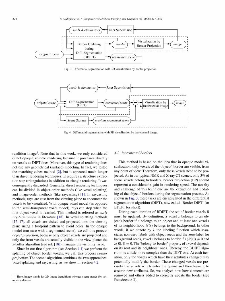
Fig. 3. Differential segmentation with 3D visualization by border projection.

Fig. 4. Differential segmentation with 3D visualization by incremental image.

rendition image1. Note that in this work, we only considereddirect opaque volume rendering because it processes directlyon voxels as DIFT does. Moreover, this type of rendering doesnot use any geometrical (surface) modeling. In fact, we testedthe marching-cubes method [2], but it appeared much longerthan direct rendering techniques: It requires a structure extrac-tion step (triangulation) in addition to triangle rendering. It wasconsequently discarded. Generally, direct rendering techniquescan be divided in object-order methods (like voxel splatting)and image-order methods (like raycasting) [1]. In raycastingmethods, rays are cast from the viewing plane to encounter thevoxels to be visualized. With opaque voxel model (as opposedto the semi-transparent voxel model), rays can stop when thefirst object voxel is reached. This method is referred as earlyray-termination in literature [18]. In voxel splatting methods[15–17], all voxels are visited and projected onto the viewingplane using a footprint pattern to avoid holes. In the opaquemodel (our case with a segmented scene), we call this processobject projection, because only object voxels are projected andonly the front voxels are actually visible in the view-plane: thez-buffer algorithm (see ref. [18]) manages the visibility issue.

Since in our first algorithm (see Section 4.1) we perform thesplatting of object border voxels, we call this process borderprojection. The second algorithm combines the two approaches,voxel splatting and raycasting, as we show in Section 4.2.

u

4.1. Incremental borders

This method is based on the idea that in opaque model vi-sualization, only voxels of the objects’ border are visible, fromany point of view. Therefore, only these voxels need to be pro-jected. As in our typical NMR and X-ray CT scenes, only 3% ofscene voxels belong to borders, border projection (BP) shouldrepresent a considerable gain in rendering speed. The noveltyand challenge of this technique are the extraction and updat-ing of the objects’ borders during the segmentation process. Asshown in Fig. 3, these tasks are encapsulated in the differentialsegmentation algorithm (DIFT), now called ‘Border DIFT’ (orBDIFT for short).

During each iteration of BDIFT, the set of border voxels Bmust be updated. By definition, a voxel s belongs to an ob-ject’s border if s belongs to an object and at least one voxel tof its neighborhood N(s) belongs to the background. In otherwords, if we denote by λ the labeling function which asso-ciates non-zero labels with object seeds and the zero-label forbackground seeds, voxel s belongs to border if λ(R[s]) �= 0 andλ(R[t]) = 0. The ‘belong-to-border’ property of a voxel dependson its root and its neighbors’ ones. Thereby, the BDIFT algo-rithm is a little more complex than the DIFT one. At each iter-ation, only the voxels which have their attributes changed maypotentially modify the border. These changed voxels are pre-cisely the voxels which enter the queue and then leave it toarP

1 Here, image stands for 2D image (rendition) whereas scene stands for vol-metric dataset.

ssume new attributes. So, we analyze now how elements areemoved and others added to correctly update the border (seeseudocode 3).


Initialization (l. 1–4) and TreeRemoval are the same asin DIFT algorithm. Yet, observe that when inserting seeds andfrontier voxels in the queue Q, we systematically remove theseelements from the border set B (l. 5) because we will test whetherthey actually belong to the border when removed from the queue.Similarly in the main loop (l. 6–19), when a voxel is insertedin the queue, it is removed from border (l. 15). The propagationprinciples are identical as in DIFT: when a voxel s leaves thequeue, if its neighbor t has not yet its definitive attributes, s triesto propagate its root (l. 9–16). Cost c of the candidate path isevaluated and proposed to t. If c is lower than the current cost orif the predecessor of t is s, attributes of t are updated (l. 11–15): thas been ‘dominated’ by a new root. Else, it is a ‘brave resister’ to‘invasion’ and is inserted in set A if not in the queue (l. 16). On theother hand, when the neighbor t of s has already a definitive value(e(t) = DONE), it is possible to test if s or t belongs to border(l. 17–19). If the belong-to-border property is satisfied for s, it isinserted in the border, else, the border test is applied to t. After themain loop, a BDIFT-specific loop must be processed (l. 20–22).Border tests are applied to the resistant voxels. These resistersare voxels which did not enter the queue because their costswere optimal. Although their attributes did not change, thesevoxels can affect the border set because they may be neighbors ofchanged voxels (the dominated). For example, it may occur that aformer object-voxel s has been dominated by a new background-root but its neighbor t has resisted and remains as an object-voxel.Imleet

4

rAartts

asdtpcg(awtmc

object-order techniques (see Pseudocode 4).

For each voxel s, previous and current associated label scenesare compared (Li−1[s] and Li[s], respectively). If s has a newlabel (see l. 3), function VoxelProject(s) computes its pro-jittipisaittDtatfTc

vpp

5

wavL

t is clear that t has become a border voxel, but nothing in theain loop can manage this exception. Indeed, during the main

oop this resister does not enter the queue but could potentiallynter it. While the main loop has not finished, there is no way tovaluate t or, by reciprocity, s belong-to-border property, becauseis never considered as a definitively valued voxel.

.2. Incremental image (II)

This second strategy of visualization aims to build an imageendition incrementally, as the DIFT builds a segmented scene.ssuming a fixed point of view between two successive iter-

tions of DIFT, we can state that the differences between theespective images (projective views) of a scene are only due tohe changes occurred in voxels’ labels (and not to scene rota-ion). The main idea of this method is to analyze changes inegmentation to update the image, as shown in Fig. 4.

Consider Li and Li−1 the labeled scenes by the λ functions the current and previous segmentation results of two sub-equent iterations. In the current iteration, a voxel may eitherisappear or appear in the image rendition. In the former case,he voxel s assumes a background label (Li[s] = 0), whereas itreviously assumed an object label (Li−1[s] �= 0). In the latterase, two situations are possible: s previously assumed a back-round label (Li−1[s] = 0) and now assumes an object labelLi[s] �= 0), or it simply changed of object (Li−1[s] = l1 �= 0nd Li[s] = l2 �= 0). Note that to distinguish objects of interest,e generally assign one color to each object. Consequently, al-

hough the voxel of the latter situation remains visible, the imageust be updated with respect to the color map. To handle these

ases, we propose a hybrid algorithm mixing image-order and

ection onto the viewing plane, according to the given visual-zation angles and returns the distance d between the voxel andhe plane as well as the corresponding image pixel p (l. 4). Inhe case of an ‘appeared’ voxel s (l2 �= 0, l. 5–6), if this voxels closer to the image plane than the voxel that was previouslyrojected into pixel p, the depth-buffer D and the visible voxelndex map V are updated. In the case of a ‘disappeared’ voxel(l. 7–8), we must verify if s was visible in the previous iter-

tion. If so, we must look for the voxel that is visible at thisteration. For this purpose, we cast a ray from the pixel p intohe labeled scene Li, according to the fixed visualization angles,o encounter an object voxel (with non-zero label). Depth-buffer

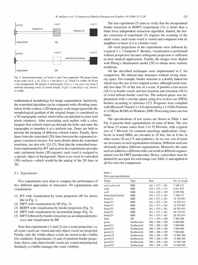
and visible voxel index map V are updated accordingly. Notehat the raycasting executed by function dRaycast(q, Li, d) isn optimized version: the ray is directly cast at a distance d fromhe image plane (i.e. at the position of s), as we know that theuture visible voxel is necessarily beyond the disappeared one.his hybrid method allows to correctly perform three types ofhanges in any order (see Fig. 5).

Note that a footprint F is used for splatting voxels onto theiewing plane. In both cases, we have to check and update allixels q in the footprint F (p) of p (see l. 5 and 7), not simplyixel p.

. Experiments and results

In all experiments, we used the watershed and differentialatershed transforms, special instances of the IFT and DIFT

lgorithms for fmax with δ(s, t) equal to a gradient intensity atoxel t. The watershed approach, first introduced by Beucher,antuejoul and Meyer [22,23], is a simple yet powerful tool of


Fig. 5. Incremental image. (a) Voxels 1 and 2 have appeared. We project themin any order. As d1 ≤ d2, V [p] = 1 and D[p] = d1. Voxel 1 is visible. (b) Voxel1 has disappeared. We project it and because V [p] = 1 we cast a ray from ituntil the remaining voxel 2 is found. Finally, V [p] = 2 and D[p] = d2. Voxel 2is visible.

mathematical morphology for image segmentation. Intuitively,the watershed algorithm can be compared with a flooding simu-lation. In this context, a 2D input gray-scale image (generally themorphological gradient of the original image) is considered asa 3D topographic surface where holes are punched at some seedpixels (markers). After associating each marker with a color,imagine that colored waters go through the holes and enter thetopography to inundate it at a uniform rate. Dams are built toprevent the merging of different colored waters. Finally, thesedams form the watershed (2D) lines between the segmented re-gions (catchment basins). For more details about the watershedtransform, see also refs. [24,25]. Note that the watershed trans-form implemented by IFT and used in the experiments providesonly catchment basins (3D regions): each voxel is assigned toa specific object or background. There is no voxel in watershed(3D) surfaces—which would be the analog of the 2D lines in3D.

5.1. Experiments

Five experiments were done to compare the performance offive different approaches of interactive 3D segmentation andvisualization:

(1) IFT with visualization by scene projection (SP for short),like in Fig. 1;

((((

aF(tS

The last experiment (5) aims to verify that the encapsulatedborder extraction in BDIFT (experiment (3)) is faster than abrute force independent extraction algorithm. Indeed, the bor-der extraction of experiment (5) requires the scanning of theentire scene: each scene voxel is visited and compared with itsneighbors to know if it is a border voxel.

All voxel projections in the experiments were followed bya typical 3× 3 footprint F. Besides, visualization is performedwithout perspective because orthogonal projection is sufficientin most medical applications. Finally, the images were shadedwith Phong’s illumination model [26] to obtain more realisticrenditions.

All the described techniques were implemented in C forcomparison. We utilized data structures without saving mem-ory space. For example, border structure is a doubly linked listwhich uses the size of two original scenes, although needs actu-ally less than 3% of the size of a scene. It permits a fast access(O(1)) to border voxels and fast insertion and remotion (O(1))of voxel in/from border voxel list. The ordered queue was im-plemented with a circular queue using first-in-first-out (FIFO)buckets according to reference [27]. Programs were compiledwith Microsoft Visual C++ 6.0 and tested by a 2.4 GHz Pentium4 (1 GBytes RAM) on Windows 2000. Processing times are realtimes.

The specifications of test scenes are shown in Table 1 andFig. 6 presents final segmentations of some of them. The sizeof these 23 scenes varies from 3 to 32 Mvoxels, with a typicalsize of 7 Mvoxels for common neurology applications. Gray-levels in tested MRIs are encoded in 16 bits, but in 8 bits inother scenes (X-ray CT and synthetic). As we saw, sets of seedsare necessary at each segmentation iteration. Different seed setsobviously produce different segmentation. Moreover, the sameseed set added in a different order can result in different segmen-tations (see the DIFT pseudocode). Hence, a procedure must bedefined by an expert for each image (see Table 2) and applied inall five tests for comparison.

Table 1Test scene specifications

Name Type Size No. of voxels

scn1,scn2,scn3 MRI 181× 217× 181 7 109 137scn4 MRI 225× 175× 173 6 811 875scn5 MRI 234× 183× 195 8 350 290brain,brain2,brain3 MRI 181× 217× 181 7 109 137brain211 MRI 361× 217× 181 14 178 997brain121 MRI 181× 433× 181 14 185 513brain112 MRI 181× 217× 361 14 178 997brain122 MRI 181× 433× 361 28 292 653brain212 MRI 361× 217× 361 28 279 657brain221 MRI 361× 433× 181 28 292 653knee XR 171× 193× 100 3 300 300geom Synthesized 200× 200× 100 4 000 000geom211 Synthesized 399× 200× 100 7 980 000geom121 Synthesized 200× 399× 100 7 980 000geom112 Synthesized 200× 200× 199 7 960 000geom122 Synthesized 200× 399× 199 15 880 200geom212 Synthesized 399× 200× 199 15 880 200geom221 Synthesized 399× 399× 100 15 920 100geom222 Synthesized 399× 399× 199 31 680 999

2) DIFT with visualization by SP (Fig. 2);3) BDIFT with visualization by border projection (Fig. 3);4) DIFT with visualization by incremental image (Fig. 4);5) DIFT followed by border extraction (as an independent pro-

cess) and visualization by BP.

Note that experiments (1) and (2) use a scene projection, i.e.ll scene voxels are visited and only object voxels are projected.inally, only the visible object voxels are stored in the z-bufferfor rendition). Experiments (3) and (5) perform border projec-ions, that is, only object border voxels are visited and projected.imilarly, a z-buffer manages the voxel visibility.


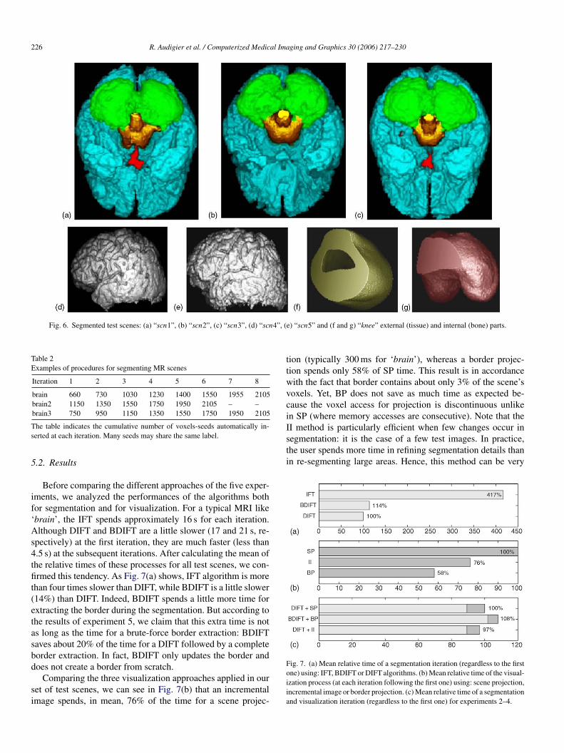
Fig. 6. Segmented test scenes: (a) “scn1”, (b) “scn2”, (c) “scn3”, (d) “scn4”, (e) “scn5” and (f and g) “knee” external (tissue) and internal (bone) parts.

Table 2Examples of procedures for segmenting MR scenes

Iteration 1 2 3 4 5 6 7 8

brain 660 730 1030 1230 1400 1550 1955 2105brain2 1150 1350 1550 1750 1950 2105 – –brain3 750 950 1150 1350 1550 1750 1950 2105

The table indicates the cumulative number of voxels-seeds automatically in-serted at each iteration. Many seeds may share the same label.

5.2. Results

Before comparing the different approaches of the five exper-iments, we analyzed the performances of the algorithms bothfor segmentation and for visualization. For a typical MRI like‘brain’, the IFT spends approximately 16 s for each iteration.Although DIFT and BDIFT are a little slower (17 and 21 s, re-spectively) at the first iteration, they are much faster (less than4.5 s) at the subsequent iterations. After calculating the mean ofthe relative times of these processes for all test scenes, we con-firmed this tendency. As Fig. 7(a) shows, IFT algorithm is morethan four times slower than DIFT, while BDIFT is a little slower(14%) than DIFT. Indeed, BDIFT spends a little more time forextracting the border during the segmentation. But according tothe results of experiment 5, we claim that this extra time is notas long as the time for a brute-force border extraction: BDIFTsaves about 20% of the time for a DIFT followed by a completeborder extraction. In fact, BDIFT only updates the border anddoes not create a border from scratch.

Comparing the three visualization approaches applied in ourset of test scenes, we can see in Fig. 7(b) that an incrementalimage spends, in mean, 76% of the time for a scene projec-

tion (typically 300 ms for ‘brain’), whereas a border projec-tion spends only 58% of SP time. This result is in accordancewith the fact that border contains about only 3% of the scene’svoxels. Yet, BP does not save as much time as expected be-cause the voxel access for projection is discontinuous unlikein SP (where memory accesses are consecutive). Note that theII method is particularly efficient when few changes occur insegmentation: it is the case of a few test images. In practice,the user spends more time in refining segmentation details thanin re-segmenting large areas. Hence, this method can be very

Fig. 7. (a) Mean relative time of a segmentation iteration (regardless to the firstone) using: IFT, BDIFT or DIFT algorithms. (b) Mean relative time of the visual-ization process (at each iteration following the first one) using: scene projection,incremental image or border projection. (c) Mean relative time of a segmentationand visualization iteration (regardless to the first one) for experiments 2–4.


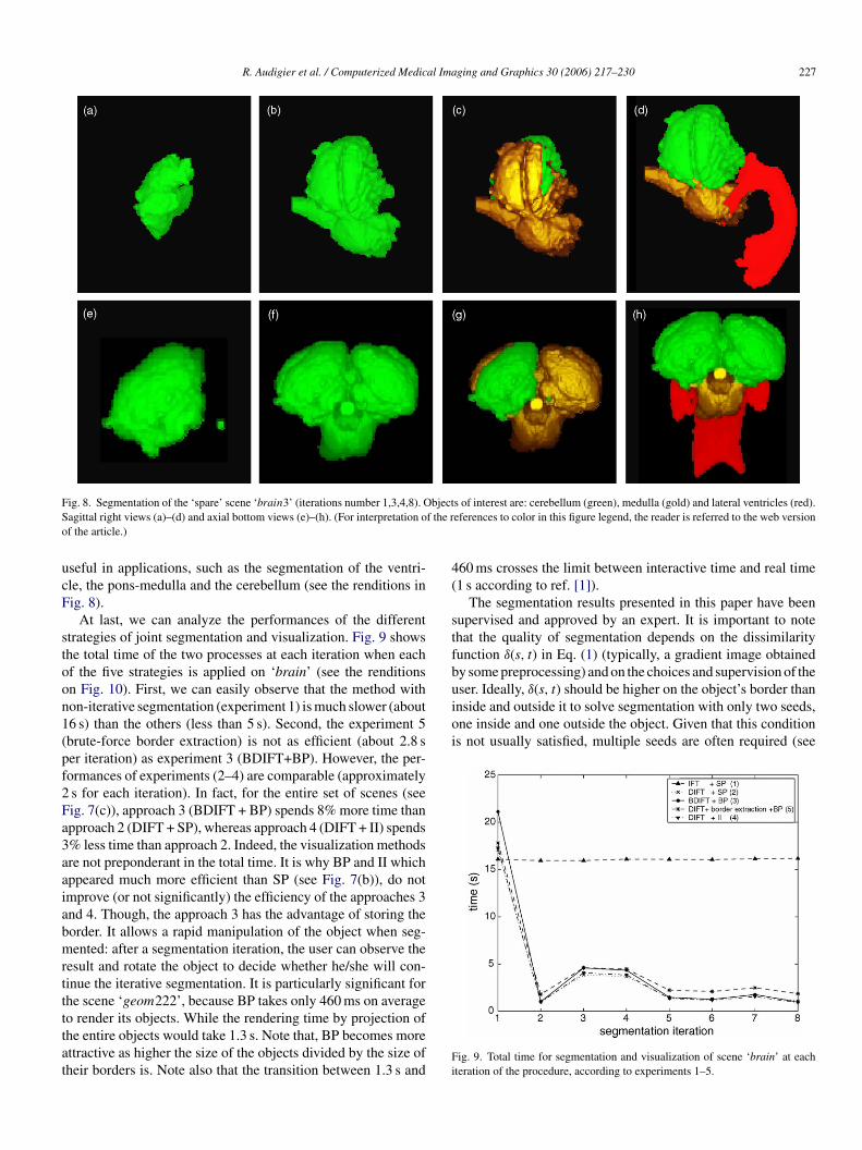
Fig. 8. Segmentation of the ‘spare’ scene ‘brain3’ (iterations number 1,3,4,8). Objects of interest are: cerebellum (green), medulla (gold) and lateral ventricles (red).Sagittal right views (a)–(d) and axial bottom views (e)–(h). (For interpretation of the references to color in this figure legend, the reader is referred to the web versionof the article.)

useful in applications, such as the segmentation of the ventri-cle, the pons-medulla and the cerebellum (see the renditions inFig. 8).

At last, we can analyze the performances of the differentstrategies of joint segmentation and visualization. Fig. 9 showsthe total time of the two processes at each iteration when eachof the five strategies is applied on ‘brain’ (see the renditionson Fig. 10). First, we can easily observe that the method withnon-iterative segmentation (experiment 1) is much slower (about16 s) than the others (less than 5 s). Second, the experiment 5(brute-force border extraction) is not as efficient (about 2.8 sper iteration) as experiment 3 (BDIFT+BP). However, the per-formances of experiments (2–4) are comparable (approximately2 s for each iteration). In fact, for the entire set of scenes (seeFig. 7(c)), approach 3 (BDIFT + BP) spends 8% more time thanapproach 2 (DIFT + SP), whereas approach 4 (DIFT + II) spends3% less time than approach 2. Indeed, the visualization methodsare not preponderant in the total time. It is why BP and II whichappeared much more efficient than SP (see Fig. 7(b)), do notimprove (or not significantly) the efficiency of the approaches 3and 4. Though, the approach 3 has the advantage of storing theborder. It allows a rapid manipulation of the object when seg-mented: after a segmentation iteration, the user can observe theresult and rotate the object to decide whether he/she will con-tinue the iterative segmentation. It is particularly significant forthe scene ‘geom222’, because BP takes only 460 ms on averagettat

460 ms crosses the limit between interactive time and real time(1 s according to ref. [1]).

The segmentation results presented in this paper have beensupervised and approved by an expert. It is important to notethat the quality of segmentation depends on the dissimilarityfunction δ(s, t) in Eq. (1) (typically, a gradient image obtainedby some preprocessing) and on the choices and supervision of theuser. Ideally, δ(s, t) should be higher on the object’s border thaninside and outside it to solve segmentation with only two seeds,one inside and one outside the object. Given that this conditionis not usually satisfied, multiple seeds are often required (see

Fig. 9. Total time for segmentation and visualization of scene ‘brain’ at eachiteration of the procedure, according to experiments 1–5.

o render its objects. While the rendering time by projection ofhe entire objects would take 1.3 s. Note that, BP becomes morettractive as higher the size of the objects divided by the size ofheir borders is. Note also that the transition between 1.3 s and


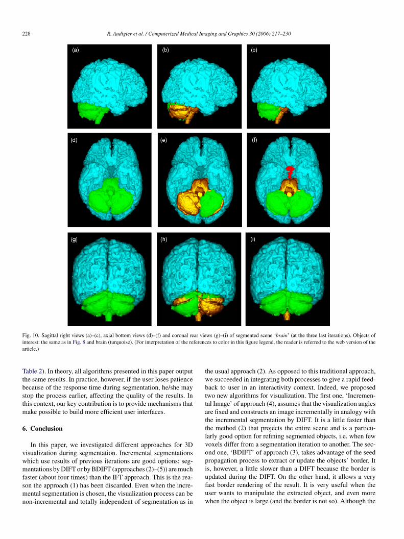
Fig. 10. Sagittal right views (a)–(c), axial bottom views (d)–(f) and coronal rear views (g)–(i) of segmented scene ‘brain’ (at the three last iterations). Objects ofinterest: the same as in Fig. 8 and brain (turquoise). (For interpretation of the references to color in this figure legend, the reader is referred to the web version of thearticle.)

Table 2). In theory, all algorithms presented in this paper outputthe same results. In practice, however, if the user loses patiencebecause of the response time during segmentation, he/she maystop the process earlier, affecting the quality of the results. Inthis context, our key contribution is to provide mechanisms thatmake possible to build more efficient user interfaces.

6. Conclusion

In this paper, we investigated different approaches for 3Dvisualization during segmentation. Incremental segmentationswhich use results of previous iterations are good options: seg-mentations by DIFT or by BDIFT (approaches (2)–(5)) are muchfaster (about four times) than the IFT approach. This is the rea-son the approach (1) has been discarded. Even when the incre-mental segmentation is chosen, the visualization process can benon-incremental and totally independent of segmentation as in

the usual approach (2). As opposed to this traditional approach,we succeeded in integrating both processes to give a rapid feed-back to user in an interactivity context. Indeed, we proposedtwo new algorithms for visualization. The first one, ‘Incremen-tal Image’ of approach (4), assumes that the visualization anglesare fixed and constructs an image incrementally in analogy withthe incremental segmentation by DIFT. It is a little faster thanthe method (2) that projects the entire scene and is a particu-larly good option for refining segmented objects, i.e. when fewvoxels differ from a segmentation iteration to another. The sec-ond one, ‘BDIFT’ of approach (3), takes advantage of the seedpropagation process to extract or update the objects’ border. Itis, however, a little slower than a DIFT because the border isupdated during the DIFT. On the other hand, it allows a veryfast border rendering of the result. It is very useful when theuser wants to manipulate the extracted object, and even morewhen the object is large (and the border is not so). Although the


border has much less voxels than the whole scene, border pro-jection is not so much faster because of random memory accesstimes. In scene projection, continuous scanning optimizes thememory access time. Perhaps, implementations of other borderdata structures would accelerate border projection.

Nowadays it can appear still better to separate both processesof segmentation and visualization for sake of simplicity. How-ever, the two other proposed methods are also satisfactory. More-over, they are very useful for huge size scenes with very highresolution as it is the case of the future generation’s medicalscanners. Furthermore, as medical imaging devices are generat-ing ever higher resolution scenes, the novel merging of segmen-tation with visualization proposed here will constitute a hot topicof research in the future. Transversal research between graphicsand image processing domains will be necessary.

Finally, this attempt of integrating both processes leads us tolarger questions about interactive segmentation: how to improveinteractivity? And how to improve a supervised segmentation?Other indicators than the visual feedback could guide the userin the iterative segmentation process. For example, volume, sur-face, connected components and use of atlas could help the userchoose new seeds and decide whether or not the segmentationis acceptable. These indicators would be more objective for theuser than a sole (subjective) observation of an image. The presentintegration of visualization and segmentation showed that onecan take advantage of segmentation process by processing mean-wihbc

A

Up3

R

[8] Drebin RA, Carpenter L, Hanrahan P. Volume rendering. SIGGRAPHComput Graph 1988;22(4):65–74.

[9] Kindlmann G, Durkin JW. Semi-automatic generation of transfer functionsfor direct volume rendering. in: IEEE Symposium on Volume Visualiza-tion. Research Triangle Park (NC), EUA; 1998. p. 79–86 [available onhttp://www.citeseer.nj.nec.com/kindlmann98semiautomatic.html].

[10] Kniss J, Kindlmann G, Hansen C. Multidimensional transfer functionsfor interactive volume rendering. IEEE Trans Visual Comput Graph2002;8(3):270–85.

[11] Cendes F, Andermann F, Gloor P, Evans A, Jones-Gotman M, Watson C,et al. MRI volumetric measurements of amygdala and hippocampus intemporal lobe epilepsy. Neurology 1993;43(4):719–25.

[12] Demarco FA, Ghizoni E, Kobayashi E, Cendes F. Cerebelar volume andlong term use of phenytoin: MRI volumetric studies. Seizure 2003;12:312–15.

[13] Falcao A, Bergo F. Interactive volume segmentation with differential imageforesting transforms. IEEE Trans Medical Imaging 2004;23(9):1100–8.

[14] Falcao A, Stolfi J, Lotufo R. The image foresting transform: theory,algorithms, and applications. IEEE Trans Pattern Anal Machine Intell2004;26(1):19–29.

[15] Westover L. Footprint evaluation for volume rendering. in: Proceedings ofSIGGRAPH; 1990. p. 367–76.

[16] Huang J, Mueller K, Shareef N, Crawfis R. Fastsplats: optimized splattingon rectilinear grids. in: IEEE Visualization. Salt-Lake City; 2000. p. 219–27.

[17] Zwicker M, Pfister H, van Barr J, Gross M. Ewa splatting. IEEE VisualComput Graph 2002;8(3):223–38.

[18] Foley J, van Dam A, Feiner S, Hughes J. Computer graphics: prin-ciples and practice. 2nd ed. New York (NY), EUA: Addison-Wesley;1990.

[19] Audigier R, Lotufo R, Falcao A. On integrating iterative segmentation

[

[

[

[

[

[

[

[

RNdt(DUim

hile data for visualization and, why not, for determining newndicators which would assist the user in segmenting, givingim/her more feedback: data analysis and visualization for aetter segmentation of the objects of interest. Again, this en-ourages research on this ‘integration’ topic.

cknowledgments

We would like to thank the Department of Neurology, Stateniversity of Campinas for the medical images used in the ex-eriments. The authors are also grateful to CAPES, CNPq (Proc.02427/04-0) and FAPESP (Proc. 03/13424-1).

eferences

[1] Udupa J, Herman G. 3D imaging in medicine. Boca Raton (Florida), USA:CRC Press; 1991.

[2] Lorensen W, Cline H. Marching cubes: a high resolution 3D surface con-struction algorithm. Comput Graph 1987;21(4):163–9 [In Proc of ACMSIGGRAPH]

[3] Udupa J, Odhner D. Shell rendering. IEEE Comput Graph Appl1993;13(6):58–67.

[4] Bentum M. Interactive visualization of volume data. Ph.D. thesis. En-schede, The Netherlands: Department of Electrical Engeneering, Univer-sity of Twente; June 1996.

[5] Pfister H, Hardenbergh J, K J, Lauer H, Seiler L. The volumepro real-timeray-casting system. ACM Comput Graph 1999:251–60 [In Proceedings ofSIGGRAPH’99].

[6] Levoy M. Volume rendering by adaptive refinement. Vis Comput1990;6(1):2–7.

[7] Danskin J, Hanrahan P. Fast algorithms for volume ray tracing. in: Pro-ceedings of the 1992 Workshop on volume rendering, vol. 19; 1992. p.91–8.

by watershed with tridimensional visualization of MRIs. in: IEEE Pro-ceedings of the XVII Brazilian Symposium on Computer Graphics andImage Processing (SIBGRAPI’04). Curitiba, Brazil: IEEE Press; 2004.p.130–7.

20] Lotufo R, Falcao A. The ordered queue and the optimality of the watershedapproaches. Fifth International Symposium on mathematical morphology;2000. p. 341–50.

21] Dijkstra E. A note on two problems in connexion with graphs. NumerischeMathematik; 1959;1:269–71.

22] Beucher S, Lantuejoul C , Use of watersheds in contour detection, in:International Workshop on image processing, real-time edge and motiondetection/estimation. Rennes, France; 1979.

23] Beucher S, Meyer F. The morphological approach to segmentation: thewatershed transform. In: Dougherty ER, editor. Mathematical morphologyin image processing. New York (NY), USA: Marcel Dekker Inc.; 1993. p.433–81.

24] Dougherty E, Lotufo R. Hands-on morphological image processing.Bellingham (Washington), USA: SPIE-The International Society for Op-tical Engineering; 2003.

25] Meyer F, Beucher S. Morphological segmentation. J Vis Commun ImageProcess 1990;1(1):21–46.

26] Phong BT. Illumination for computer generated pictures. Commun ACM1975;18:311–17.

27] Falcao A, Udupa J, Miyazawa F. An ultra-fast user-steered imagesegmentation paradigm: live-wire-on-the-fly. IEEE Trans Med Imaging2000;19(1):55–62.

omaric Audigier received the Electrical Engineering Diploma from Institutational des Sciences Appliquees (INSA) of Lyon, France, in 2001, the M.Sc.egree in Images and Systems from École Doctorale EEA of Lyon, in 2001, andhe M.Sc. degree in Electrical Engineering from the State University of CampinasUNICAMP), SP, Brazil, in 2004. Since 2004, he has been a Ph.D. student in theepartment of Computer Engineering and Industrial Automation at the Stateniversity of Campinas (UNICAMP), SP, Brazil. His research interests include

mage processing and analysis, mathematical morphology, image segmentation,edical imaging and volume visualization.

http://www.citeseer.nj.nec.com/kindlmann98semiautomatic.html


Roberto A. Lotufo obtained the Electronic Engineering Diploma from InstitutoTecnologico de Aeronautica, Brazil, in 1978, the M.Sc. degree from the Uni-versity of Campinas, UNICAMP, Brazil, in 1981, and the Ph.D. degree fromthe University of Bristol, U.K., in 1990, in Electrical Engineering. He is a fullprofessor at the School of Electrical and Computer Engineering, University ofCampinas (UNICAMP), Brazil, were he has worked for since 1981. His princi-pal interests are in the areas of Image Processing and Analysis, MathematicalMorphology, Image Segmentation and Medical Imaging. He is one of the mainarchitects of two morphological toolboxes: MMach for Khoros, and SDC Mor-phology Toolbox for MATLAB. He is the executive director of Inova Unicamp,the agency for innovation at Unicamp, since 2004. Prof. Lotufo has publishedover 50 refereed international journal and full conference papers.

Alexandre Xavier Falcao received a B.Sc. in Electrical Engineering fromthe Federal University of Pernambuco, Recife, PE, Brazil, in 1988. He has

worked in medical image processing, visualization and analysis since 1991.In 1993, he received a M.Sc. in Electrical Engineering from the State Univer-sity of Campinas, Campinas, SP, Brazil. During 1994-1996, he worked withthe Medical Image Processing Group at the Department of Radiology, Uni-versity of Pennsylvania, PA, USA, on interactive image segmentation for hisdoctorate. He got his doctorate in Electrical Engineering from the State Univer-sity of Campinas in 1996. In 1997, he worked in a research center (CPqD-TELEBRAS, Campinas) developing methods for video quality assessment.His experience as professor of Computer Science and Engineering started in1998 at the State University of Campinas, where he is currently an Asso-ciate Professor (since 2003). His main research interests include image seg-mentation and analysis, volume visualization, content-based image retrieval,mathematical morphology, digital video processing and biomedical imagingapplications.

3D visualization to assist iterative object definition from medical images

Documents

Transcript of 3D visualization to assist iterative object definition from medical images