3.5 GHz Coverage Assessment with a 5G TestbedAdrian Schumacher*#, Ruben Merz* and Andreas Burg#

*Enterprise Architecture & Innovation, Swisscom Ltd., CH-3050 Bern, Switzerland{adrian.schumacher,ruben.merz}@swisscom.com

#Telecommunications Circuits Laboratory, EPFL, CH-1015 Lausanne, Switzerlandandreas.burg@epfl.ch

©2019 IEEE. Personal use of this material is permitted. Permission from IEEE must be obtained for all other uses, in any current or future media, includingreprinting/republishing this material for advertising or promotional purposes, creating new collective works, for resale or redistribution to servers or lists, orreuse of any copyrighted component of this work in other works. DOI: 10.1109/VTCSpring.2019.8746551

Abstract—Today, cellular networks have saturated frequenciesbelow 3 GHz. Because of increasing capacity requirements, 5thgeneration (5G) mobile networks target the 3.5 GHz band (3.4 to3.8 GHz). Despite its expected wide usage, there is little empiricalpath loss data and mobile radio network planning experiencefor the 3.5 GHz band available. This paper presents the resultsof rural, suburban, and urban measurement campaigns using apre-standard 5G prototype testbed operating at 3.5 GHz, withoutdoor as well as outdoor-to-indoor scenarios. Based on themeasurement results, path loss models are evaluated, which areessential for network planning.

Index Terms—5G, sub-6 GHz, 3.5 GHz, propagation measure-ments, beamforming

I. INTRODUCTION

The global demand for higher-capacity mobile Internet ser-vices drives the continuous evolution of mobile (cellular) tech-nologies. Up until the 4th generation mobile network (4G,also commonly known as Long Term Evolution (LTE)), onlyfrequency bands up to around 2.7 GHz have been used (with afew exceptions). To carry the required increase in data capacity,more bandwidth in higher frequency spectrum is required.CEPT/ECC identified1 the 3400–3800 MHz frequency band tobe harmonized in Europe for 5G usage, along with the 24.25–27.5 GHz band. National regulators already have made, or are inthe process of making the 3.4–3.8 GHz (referred to as 3.5 GHz)band available for mobile network operators. For instance, inSwitzerland, an auction for this band was conducted duringthe first quarter of 2019. With 5G, we refer to the Release 15New Radio (NR) standard by the 3rd Generation PartnershipProject (3GPP). 5G NR is frequency band agnostic and couldbe deployed on legacy bands (below 3 GHz), but also in themilimeter-wave (mmWave) spectrum. As a compromise to stillhave fairly good propagation properties, but also allow forwider carrier bandwidths, the 3.5 GHz band is of particularinterest among the bands below 6 GHz (sub-6 GHz). Propagationchannels for mobile use in the 3.5 GHz band and above, havemainly been studied in the context of WiMAX (Worldwideinteroperability of Microwave Access) and with less carrierbandwidth compared to what 5G will be able to use (up to200 MHz carrier bandwidth for sub-6 GHz). It also needs to beconsidered that an increase in bandwidth requires the same factorfor a power increase, to maintain the same coverage area.

For radio network planning, propagation models are used,which can be categorized into deterministic, stochastic,empirical, and standardized models [1, Chapter 4]. While

1https://www.cept.org/ecc/topics/spectrum-for-wireless-broadband-5g

deterministic models (e.g., ray tracing) may yield accurateresults, they require a high degree of detailed descriptionand calibration of the environment and are computationallyexpensive. Stochastic models (e.g., COST 207) employrandom variables and do not require much information aboutthe environment, but also cannot provide high-accuracypath loss predictions. Empirical (e.g., Hata-Okumura) andstandardized models are based on measurements and have beenwidely adopted to predict a mean path loss as a function ofdistance, frequency, and some further parameters specific tothe environment or infrastructure. They require also only a fewparameters and can provide an acceptable prediction accuracy,better than the very general and simplified path loss model (1).For these reasons, radio network planners in the industry oftenuse empirical path loss models for network planning simulations.

A. Overview of Empirical Path Loss ModelsBecause most mobile communications applications use fre-

quencies up to around 2 GHz, the empirical path loss modelswere optimized to cover only these frequencies. Examples are(see also Table I): Hata-Okumura [2], COST 231 Hata [3],COST 231 Walfish-Ikegami (COST 231 WI) [3], and Erceg [4].Path loss models valid for the 3.5 GHz band are the StanfordUniversity Interim (SUI) IEEE 802.16 model [5] which is anextension to the Erceg model, the ECC-33 model [6] whichextrapolates the Hata-Okumura model, the WINNER II models[7], the ITU-R P.1411-9 models [8], as well as the 3GPP modelsdescribed in [9].

When designing wireless networks, it is obvious that underes-timating the path loss can lead to coverage holes. However, alsooverestimating the path loss is undesirable because this leads tosevere inter-cell interference issues. For an accurate prediction,existing models need to be evaluated for the environments inwhich they shall be used and adjusted if necessary. Additionally,penetration of signals from outdoor to indoor is dependingheavily on the building materials and is varying a lot, even withinthe same cell coverage area. While wooden and older houses –Rec. ITU-R P.2109-0 [10] refers to ‘traditional buildings’ – tendto have a small penetration loss, modern ‘thermally-efficient’buildings with infrared light reflecting low emissivity (low-e)coated glass windows impose high losses.

In general the path loss (in dB) can be expressed according tothe simplified model in [1, eq. (1.12)]:

PL(d) = A0 + 10γ log10 (d/d0) + χσ d > d0, (1)

where A0 represents the deterministic path loss component atthe reference distance d0 in meters. The path loss exponent is

arX

iv:2

105.

0681

2v1

[cs

.NI]

14

May

202

1

TABLE ISELECTED EMPIRICAL PATH LOSS MODELS

Name Frequency Range Distance Range

Hata-Okumura 150− 1500MHz 1− 20 kmCOST 231 Hata 1500− 2000MHz 1− 20 kmCOST 231 Walfish-Ikegami 800− 2000MHz 0.02− 5 kmErceg ≈ 2000MHz 0.1− 8 kmSUI IEEE 802.16 1− 4GHz 0.1− 8 kmECC-33 3.4− 3.8GHz 1− 10 kmWINNER II 2− 6GHz 0.05− 5 kmITU-R P.1411-9 0.3− 100GHz 0.055− 1.2 km3GPP 0.5− 100GHz 0.01− 5∗ km∗10 km for RMa LOS

denoted γ and d is the distance in meters between base station(BS) and user equipment (UE). Finally, χσ is the stochasticshadow fading component in dB with a zero-mean log-normaldistribution and standard deviation σ. The above mentionedempirical models can also be expressed according to (1) withadditional terms depending on, e.g., the operating frequency,BS and/or UE antenna height, etc. [11, eqs. (3)–(12)].

B. Related Work

Before 5G, there was already an interest in the 3.5 GHz bandin the early 2000’s with the radio access technology WiMAX forfixed wireless access. Therefore, several measurement results areavailable for the frequency range 3.4–3.8 GHz, e.g., [11], [12],[13], [14], [15]. The corresponding measurement campaigns ei-ther used a WiMAX system with a signal bandwidth of 3.5 MHz,or a continuous wave (CW) signal. Therefore, no conclusions canbe drawn confidently for a wide bandwidth such as 100 MHz thatcan be used for 5G. The BS antenna height varied between 15–36 m, while the UE antenna height varied between 2–10 m aboveground. Some comparisons have been done with the modelsErceg, COST 231 WI, COST 231 Hata, SUI, and ECC-33, butnone with 3GPP’s path loss models. All publications calculateda path loss exponent and standard deviation according to thesimplified path loss model from (1), which are summarizedin Table II (only the lowest UE height is considered in thetable). The variations in these parameters (e.g., γ for a suburbanterrain ranges from 2.13 to 4.9 and for urban terrain from 2.3 to4.3) indicate that there are many influences on the propagationchannel that may depend on the geographic region, constructionmaterial, and vegetation which in parts has also been confirmedin [16]. While [12] suggests the ECC-33 model for urban andthe SUI (terrain B) for suburban environments, [14] found thatthe Erceg (terrain C) fits best, but underpredicts the measuredpath loss. For rural environments, [11] and [12] show that thebest fitting models SUI (terrain B & C) and COST 231 Hataoverestimate the measured path loss. Because the path loss modelwith the lowest prediction error varies, it is difficult to set on aspecific model for network planning purposes.

Regarding outdoor-to-indoor propagation, measurementswere presented in [17], along with few outdoor measurements.A difference of only 10 dB more attenuation was found for amodern building compared to an old building. According to theauthors, this stems from different wall thicknesses and buildingmaterial. Therefore we conclude that the modern building wasnot equipped with low-e coated windows.

TABLE IICOMPARISON OF PATH LOSS PARAMETERS FOR (1) AT 3.5 GHZ

Terrain Location UE Height Distance γ σ[m] [m] [dB]

rural Cambridge, UK [12] 6 250-2000 2.7 10rural Piemonte, Italy [11] 2 1000-10000 2.5 8.9suburban Cambridge, UK [12] 6 250-2000 2.13 11.1suburban Ghent, Belgium [14] 2.5 30-1500 4.9 7.7suburban Shanghai, China [15] 3 300-1800 3.6 9.5urban Cambridge, UK [12] 6 250-2000 2.3 11.7urban United Kingdom [13] 2.5 100-2000 4.3 7.5

C. Contribution and Outline

The related works listed above show that the path loss char-acteristics (path loss exponent, standard deviation) vary a lotdepending on the environment. Because it is difficult to decide fora specific path loss model and do the network planning accord-ingly, we conducted extensive measurements in Switzerland in arural, suburban, and urban environment. The measurement setupand environments are described in Section II. Contrary to mostprior works, a beamforming BS antenna was used and parallelmeasurements on a live network in legacy frequency bands wereconducted for comparison and validation, and more realistic UEantenna heights for mobile cellular applications were used. Theobtained results are compared against the 3GPP, WINNER II,and SUI path loss models, and described in Section III (ITU-RP.1411-9 was excluded due to the specificity to environments).We find that most models overestimate the path loss, and forevery scenario, a different model predicts the path loss with theleast error. Finally, the paper is concluded in Section IV.

II. MEASUREMENT SETUP AND ENVIRONMENT

A. Measurement Method

The propagation path loss in the downlink is defined as theradio frequency (RF) attenuationPL in dB of a transmitted signalwhen it arrives at the receiver:

PL = PT +GT (φ, θ) +GR − PR [dB], (2)

where PT is the BS transmitted power in dBm and GT (φ, θ)the transmitter antenna gain in dB as a function of azimuthangle φ and elevation angle θ. Because the UE antenna isomnidirectional, we can simplify the receiver antenna gain asa constant GR in dB. Finally, PR is the local mean receivedpower in dBm.

For the analysis, all measurement parameters were geographi-cally binned in a two-dimensional square 5 m grid, thus removingfast fading effects according to the Lee sampling criterion [18],and to prevent a bias from temporal influences due to, e.g., stopsat red traffic lights. For each bin, the median value was computed.For the log-distance path loss plots, also the median value wascalculated for each 5 m distance bin.

B. 5G Testbed

For conducting measurements as close to 5G as possible, weemployed a 5G testbed (similar to [19]). It consists of a BSunit, an active antenna system (AAS) connected via fiber to theBS, and in our case two UEs (see Fig. 1a for a picture of theAAS and one UE). The center frequency for which test-licenses

(a) 5G Testbed (b) Rural Deployment

(c) Suburban Deployment (d) Urban Deployment

Fig. 1. (a) Shows the 5G testbed AAS on a mast and the UE in the field, (b)the map of the rural deployment with a red star indicating the AAS locationwith the 120◦ sector, and the LOS/NLOS classification. Similarly, (c) and (d)show the map of the suburban and urban deployments, respectively.

were available, was 3.55 GHz. The time division duplex (TDD)and orthogonal frequency division multiplexing (OFDM) signaloccupies a bandwidth of 80 MHz. Further details can be foundin [19, Tab. 1] and the references therein. Contrary to the beamgrid described in [19], we were using a configuration with the 48different dual-polarized beams arranged in a grid of three rowswith 16 beams each (visible in Fig. 2). The antenna gain andresulting coverage remains approximately the same as with theconfiguration described in [19] with 27 dBi, and 120◦ in azimuthand 30◦ in elevation, respectively. The two identical UEs haveeight antenna ports connected to an eight element omnidirec-tional cross-polarized antenna, each element with a gain of 6 dBi.

As in [19], the Mobility Reference Signal Received Power(MRSRP) for each of the 48 beams has been logged andused for the analysis. The Mobility Reference Signal (MRS)is a pilot signal that is used for subframe synchronizationand identification of downlink beams. It is transmitted every5 ms and cycles through all 48 beams over a period of 20 ms.Although there are significant differences such as the subcarrierbandwidth, it can be used similarly to the LTE Reference SignalReceived Power (RSRP). For each period, the highest of the 48MRSRP values is used as PR. The cable loss between the UE’sRF frontend and the UE’s antenna can be considered as part of theconstantGR, which then becomes 4 dBi. On the transmitter side,we can directly use the configured powerPT of the AAS, becausethe radio chains and power amplifiers are directly connectedwith the antenna elements. However, depending on where theUE is located with respect to the AAS, a directive antennagain GT (φ, θ) is considered. Because this is a beamformingantenna with a grid of beams, an artificial envelope pattern canbe calculated by cycling through all beams sequentially, thenvirtually overlay them, and taking the maximum at each angle,see Fig. 2. The total measurement uncertainty is 6.25 dB.

The UE has been moved around with a van, or where drivingwas not possible, pushed by hand. When using the van, the UE

0

30

6090

120

150

180

210

240270

300

330

-50

-40

-30

-20

-10

0

Azimuth

0

30

6090

120

150

180

210

240270

300

330

-50

-40

-30

-20

-10

0

Elevation

Macro Antenna, 0.8/2.1 GHz Beamforming Antenna, 3.5 GHz

Fig. 2. Antenna pattern envelope for a macro antenna and the AAS.

and scanner antennas were mounted 16 cm over the vehicle’sroof to limit its influence on the antenna characteristic, whichresulted in 2.1 m above ground. When manually pushing the UEaround, the antennas were at a height of 1.4 m above ground,corresponding to the approximate height at which an adult isusually holding a smartphone.

C. Comparison With 4G/LTE

For the analysis of the 5G cell, it is interesting to have acomparable 4G (LTE) cell available. Thus, the test deploymentswere chosen to have not only an existing macro site antenna mastfor installation of the 5G AAS, but also to have a live LTE signalon a legacy frequency band available.

For the measurements, a mobile network scanner (Rohde &Schwarz® TSMW) with a laptop running Nemo Outdoor hasbeen used to log propagation channel metrics based on theLTE downlink signal. The RF was locked to one frequencyband (800 MHz or 2.1 GHz) and all RSRP values per cell wererecorded. For the analysis, only the values of the cell(s) of interestwere used. The 2×2 MIMO antennas (Rohde & Schwarz®

TSMW-Z8) which were used, emulate omnidirectional smart-phone antennas to give realistic results. Together with the cablelosses, their gain is considered with -3 dBi each (note that smart-phone antennas are usually integrated and partially covered,leading to negative antenna gains). On the LTE base station side,the transmit power is corrected with the feeder cable losses inorder to have the transmit power PT with respect to the antennaports. Again, a directive antenna gainGT (φ, θ) is considered (seeFig. 2), depending on the relative location of the testbed UE to theLTE BS antenna. The total measurement uncertainty is 4.5 dB.

The network scanner has been fitted inside the 5G testbed UE,and the 2×2 MIMO antennas could also be mounted close to the5G antennas of the UE, without shielding them.

D. Rural Area Environment

The rural deployment was located close to a village (Meikirch)north-west of Bern, Switzerland. The selected live macro siteonly had an LTE 800 MHz cell with a 10 MHz carrier directedover flat open fields towards a village at 1–1.5 km distance. The5G AAS was installed right below the live macro antenna at aheight of 12.4 m above ground, with the same azimuth angle asthe macro antenna. The vertical separation of the macro antennato the testbed AAS was 2.1 m, which resulted in a mean elevationangle difference of 0.22◦ seen from the UE antenna over all

measurement sample locations. The maximum used transmitpower for 3.5 GHz was 1560WERP.

The measurements took place in mid-July 2018 during a sunnyand clear week with an air temperature of around 22◦C.

E. Suburban Area Environment

The suburban deployment was done in Ittigen, just north-eastof Bern, Switzerland, situated on a slightly ascending slope.For comparison, the signal from an existing LTE macro site at2.1 GHz with a 20 MHz carrier was used. The testbed AAS hasbeen mounted on a smaller extra mast next to the LTE macro sitemast due to space limitations on the latter. The height of the AASwas 24.5 m above ground. The horizontal separation betweenthe antennas was 3.8 m, while the vertical separation was 8.5 m.The mean angular separation of both antennas seen from the UEover all measurement sample locations is 0.232◦ in azimuth and0.819◦ in elevation and is regarded as negligible. The maximumtransmit power for 3.5 GHz had to be limited due to stringent non-ionizing radiation (NIR) regulations in Switzerland. Withoutlowering the transmit power on the live macro cells, the allowedmaximum transmit power for 3.5 GHz was 384WERP.

The measurements took place end of April and beginning ofMay 2018, with sunny and also overcast days, but no rain. Theair temperature was around 15–20◦C.

F. Urban Area Environment

For an urban deployment, a suitable and existing live macrosite was selected in the city of Zurich, Switzerland. The AAShas been mounted just below a macro sector antenna on thesame mast at a height of 29.4 m above ground, overlooking aflat part of the city. Unfortunately, due to technical issues, nomeasurements of an LTE legacy band could be taken for thisscenario. Also here, the NIR regulations required that we hadto lower the maximum transmit power. By slightly reducing thepower on a few live macro cells on this site, we were allowed touse the same maximum 384WERP for the 3.5 GHz 5G cell asin the suburban deployment.

The measurements took place middle of August 2018 duringa sunny week with an air temperature of around 25◦C.

G. Outdoor-to-Indoor Scenario

Additionally to outdoor drive and walk tests, indoor mea-surements were collected at four buildings of the suburbandeployment and two buildings of the urban deployment. The goalwas to assess the penetration loss into buildings for frequenciesabove 3 GHz. Measurements were started inside, just behind awindow with line-of-sight to the 5G AAS. The UE was thenslowly and steadily moved further inside the building, eitheruntil the connection dropped or the back side of the building wasreached. Outdoor reference measurements were either taken justin front of the building or on a terrace on top of the building.

III. MEASUREMENT RESULTS

For all environments described in the previous section, atotal of 267 data sets were analyzed. Each site deployment wasanalyzed separately, and the path loss was obtained according to(2). Using a least squares (LS) regression, the path loss exponent

TABLE IIIESTIMATED PATH LOSS MODEL PARAMETERS FOR (1)

Frequency Rural LOS/NLOS Suburban Urbanγ χσ [dB] γ χσ [dB] γ χσ [dB]

3.55 GHz 2.3 / 3.1 5.1 / 9.4 2.9 6.9 4.8 7.12.1 GHz – – 3.7 7.0 – –800 MHz 2.8 / 3.4 5.9 / 7.5 – – – –

γ is estimated with the reference distance d0 at 100 m, and thestandard deviation χσ is calculated according to the model (1).The estimated values are listed in Table III. A comparison withthe models SUI IEEE 802.16 (A, B, C), ECC-33, WINNER II(C1, C2, D1), and 3GPP (RMa, UMa) was performed. In general,the ECC-33 model overestimates the path loss and is not wellsuited because it was derived by fitting curves for distances of 1 to10 km. For the few models that agree the most with the respectivemeasurements, prediction error statistics have been computed.The mean prediction error µe indicates an over- (positive value)or under-prediction (negative value) with standard deviation σe,and the root mean square of the prediction error RMSE representsthe general metric for comparison of how well the models fitthe measurements. These were calculated in log-domain [dB].

A. Rural Environment

As expected, this environment provides a good share of line-of-sight (LOS) opportunities, in fact 42 % of the measurementsamples are estimated to be in LOS condition. The large share ofLOS makes it necessary to analyze LOS and NLOS separately.The classification for LOS/NLOS has been done by manuallydefining five coordinate polygons. All measurement sampleswithin these five polygons were categorized as LOS, the othersas NLOS. The measured path loss for 3.5 GHz is shown inFig. 3 (LOS marked with circles) with predictions from themodels 3GPP Rural Macro (RMa) NLOS and the WINNER IID1 (rural macro) NLOS. The free space path loss (FSPL) is alsoshown as a reference. Variations in the path loss from 600 mto 2 km (see shaded area) show the changes between LOS andNLOS environments. All error statistics are listed in Table IV.Both models overestimate the path loss by 14.9 dB and 9.8 dB,respectively, and the WINNER II D1 rural NLOS model fitsbest, although the measurements are often well outside of its8 dB standard deviation. The shadow fading distribution isshown in Fig. 7 in the top two distributions for LOS and NLOS.

101 102 103 104

Distance from Base Station Antenna to Mobile Station Antenna [m]

60

80

100

120

140

160

Path

Los

s [d

B]

Mix of distinctLOS and NLOS

Measurement 3.55 GHzLS Model 3.55 GHz3GPP RMa NLOSWINNER II D1 NLOSditto, = 8 dBFSPL @ 3.55 GHzMeasurement 800 MHzFSPL @ 800 MHz

Fig. 3. Rural environment measurements compared to models.

50 60 70 80 90 100 110 120 130 140 150Path Loss [dB] for 800 MHz and 2.1 GHz

60

80

100

120

140

160

Path

Los

s [d

B]

for

3.5

GH

z

Rural Measurements 3.5 GHz/800 MHzLinear fit, = 15 dB, = 8.3 dBSuburban Measurements 3.5 GHz/2.1 GHzLinear fit, = 5.8 dB, = 8.1 dB

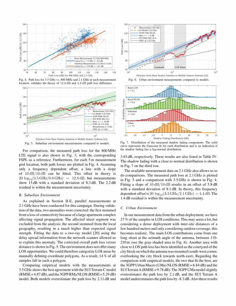
Fig. 4. Path loss for 3.5 GHz vs. 800 MHz and 2.1 GHz at each measurementlocation; validates the theory of 12.8 dB and 4.4 dB path loss difference.

102 103

Distance from Base Station Antenna to Mobile Station Antenna [m]

60

80

100

120

140

160

Path

Los

s [d

B]

Measurement 3.55 GHzLS Model 3.55 GHz3GPP RMa NLOSSUI IEEE 802.16 Cditto, = 10 dBFSPL @ 3.55 GHzMeasurement 2.1 GHzFSPL @ 2.1 GHz

Fig. 5. Suburban environment measurements compared to models.

For comparison, the measured path loss for the 800 MHzLTE signal is also shown in Fig. 3, with the correspondingFSPL as a reference. Furthermore, for each 5 m measurementgrid location, both path losses are plotted in Fig. 4. Assumingonly a frequency dependent offset, a line with a slopeof 10 dB/10 dB can be fitted. This offset in theory is20 log10(3.5GHz/0.8GHz) = 12.8 dB, but measurementsshow 15 dB with a standard deviation of 8.3 dB. The 2.2 dBresidual is within the measurement uncertainty.

B. Suburban Environment

As explained in Section II-E, parallel measurements at2.1 GHz have been conducted for this campaign. During valida-tion of the data, two anomalies were corrected: the first stemmedfrom a loss of connectivity because of a large apartment complexaffecting signal propagation. The affected street segment wasexcluded from the analysis; the second stemmed from the localgeography, resulting in a much higher than expected signalstrength. Fitting the data to a two-ray model [20] using thedelay spread information from the network scanner allowed usto explain this anomaly. The corrected overall path loss versusdistance is shown in Fig. 5. The environment does not offer manyLOS opportunities. We could therefore categorize LOS areas bymanually defining coordinate polygons. As a result, 14 % of allsamples fall in such a polygon.

Comparing empirical models with the measurements at3.5 GHz shows the best agreement with the SUI Terrain C model(RMSE = 4.87 dB), and the 3GPP RMa NLOS (RMSE = 5.29 dB)model. Both models overestimate the path loss by 2.11 dB and

101 102 103

Distance from Base Station Antenna to Mobile Station Antenna [m]

60

80

100

120

140

160

Path

Los

s [d

B]

LOS StreetCourtyard

Measurement 3.55 GHzLS Model 3.55 GHz3GPP UMa NLOSditto, = 6 dBSUI IEEE 802.16 AFSPL @ 3.55 GHz

Fig. 6. Urban environment measurements compared to models.

-25 -20 -15 -10 -5 0 5 10 15 20 25Shadow Fading Distribution [dB]

Prob

abili

ty D

ensi

ty

Rural LOS = 5.1

Rural NLOS = 9.4

Suburban = 6.9

Urban = 7.1

Fig. 7. Distribution of the measured shadow fading components. The solidcurve represents the Gaussian fit for each distribution and is an indication ifthe shadow fading has a log-normal distribution.

3.83 dB, respectively. These results are also listed in Table IV.The shadow fading with a close to normal distribution is shownin Fig. 7 on the third row.

The available measurement data on 2.1 GHz also allows us todo comparisons. The measured path loss at 2.1 GHz is plottedin Fig. 5 and a comparison with 3.5 GHz is shown in Fig. 4.Fitting a slope of 10 dB/10 dB results in an offset of 5.8 dBwith a standard deviation of 8.1 dB. In theory, this frequencydependent offset is 20 log10(3.5GHz/2.1GHz) = 4.4 dB. The1.4 dB residual is within the measurement uncertainty.

C. Urban Environment

In our measurement data from the urban deployment, we have27 % of the samples in LOS conditions. This may seem a lot, butconsidering a dense deployment with inter-site distances of afew hundred meters and only considering outdoor coverage, thisbecomes realistic. The main LOS contributions come from onelong street at the azimuth angle of the antenna, between 110-210 m (see the gray-shaded area in Fig. 6). Another area withclose to LOS path loss has been identified as the courtyard of thecity block on which the antenna was mounted (south-west corner,overlooking the city block towards north-east). Regarding thecomparison with empirical models, the two that fit the best, arethe 3GPP Urban Macro (UMa) NLOS (RMSE = 6.84 dB) and theSUI Terrain A (RMSE = 9.78 dB). The 3GPP UMa model slightlyoverestimates the path loss by 2.1 dB, and the SUI Terrain Amodel underestimates the path loss by -8.3 dB. Also these results

-60 -50 -40 -30 -20 -10 0 10

RSRP Difference to Oudoor [dB]

0

0.2

0.4

0.6

0.8

1

EC

DF

Bldg 1Bldg 2Bldg 3, low-e glassBldg 4, low-e glassBldg 5, ground floorBldg 5, 13th floorBldg 6, 6th floorBldg 6, 12th floor

non-coated

1 coatedlayer

2 or morecoated layers

Fig. 8. Outdoor-to-indoor penetration loss shown as empirical CDF of thereceived power difference from indoor compared to outdoor.

TABLE IVPATH LOSS MODEL PREDICTION ERROR STATISTICS

Environment Rural Suburban UrbanModel RMa WINNER2 RMa SUI C UMa SUI A

µe [dB] 14.9 9.82 3.83 2.11 2.07 -8.3σe [dB] 10.8 7.53 3.66 4.4 6.54 5.18RMSE 18.4 12.4 5.29 4.87 6.84 9.78

are listed in Table IV. The shadow fading distribution is shownat the bottom of Fig. 7 and conforms to the normal distribution.

D. Outdoor-to-Indoor Scenario

The indoor RSRP measurements are normalized with thecorresponding reference outdoor RSRP and the empirical cu-mulative distribution function (CDF) is plotted, see Fig. 8. Thebuildings 1–4 are from the suburban deployment, the buildings5 & 6 from the urban deployment. The measurements clearlyshow which buildings are new or with coated low-e windows,and which ones use regular windows: building 1 is an older officebuilding with regular double glazing windows. Building 2 is ahome for elderly people, also with uncoated double glazing win-dows. Building 3 is a new apartment building, with triple glazinglow-e windows, causing around 30 dB of additional loss. Build-ing 4 is a newer office building with triple glazing windows andone coated layer. Building 5 is a renovated 14 floor office build-ing. The measurements from the ground floor behind large singlelayer shop-windows show the lower attenuation than from the13th floor behind multiple glazing low-e windows. Building 6 is a12 floor renovated office building with low-e windows. The mea-surements from the 6th and 12th floor show about the same atten-uation, only walls inside the building cause different variationsin the path loss. In general, we can say that newer or renovatedbuildings with coated low-e windows add 10–30 dB of additionalpenetration loss compared with buildings with regular windows.

IV. CONCLUSIONS

Measurements from extensive rural, suburban, and urbanmeasurement campaigns with a 5G testbed operating in the3.5 GHz band have been analyzed and compared with predictionsfrom empirical path loss models (3GPP, WINNER II, SUI).Almost all models tend to overestimate the path loss. Eventhough no model gives the least error in all environments, the3GPP group of models always ranked among the top two, with anover prediction of 2.1 dB and 3.8 dB for the urban and suburban

scenario, and 14.9 dB for the rural scenario. Furthermore, theexcessive attenuation of around 10 dB per coating layer of low-ewindows has an impact on outdoor-to-indoor penetration as thenumber of newly built and renovated houses grows. Finally, pathloss exponents are slightly lower with a beamforming antenna at3.5 GHz, compared to a conventional macro antenna at 2.1 GHzand 800 MHz.

REFERENCES

[1] B. Clerckx and C. Oestges, MIMO Wireless Networks: Channels,Techniques and Standards for Multi-Antenna, Multi-User and Multi-CellSystems. Academic Press, Jan. 2013.

[2] M. Hata, “Empirical formula for propagation loss in land mobile radioservices,” IEEE Transactions on Vehicular Technology, vol. 29, no. 3,pp. 317–325, Aug. 1980.

[3] “COST Action 231: Digital mobile radio towards future generationsystems: Final Report.” European Commission, Brussels, Belgium, Tech.Rep. EUR 18957, Apr. 1999.

[4] V. Erceg, L. J. Greenstein et al., “An empirically based path lossmodel for wireless channels in suburban environments,” IEEE Journalon Selected Areas in Communications, vol. 17, no. 7, pp. 1205–1211,Jul. 1999.

[5] IEEE, “Channel Models for Fixed Wireless Applications,” IEEE, Tech.Rep. IEEE 802.16.3c-01/29r4, Jul. 2001.

[6] “The analysis of the coexistence of FWA cells in the 3.4 - 3.8GHz band,” Electronic Communication Committee (ECC) within theEuropean Conference of Postal and Telecommunications Administration(CEPT), Tech. Rep. ECC Report 33, May 2003.

[7] Pekka Kyosti, Juha Meinila et al., “WINNER II Channel Models,” Eu-ropean Commission, Tech. Rep. D1.1.2 V1.2, IST-4-027756 WINNERII Deliverable, Feb. 2008.

[8] “Propagation data and prediction methods for the planning of short-rangeoutdoor radiocommunication systems and radio local area networksin the frequency range 300 MHz to 100 GHz,” ITU-R, Tech. Rep.Recommendation P.1411-9, Jun. 2017.

[9] 3GPP, “Study on channel model for frequencies from 0.5 to 100 GHz,”3rd Generation Partnership Project (3GPP), Technical Report (TR)38.901, 06 2018, version 15.0.0.

[10] “Prediction of Building Entry Loss,” ITU-R, Tech. Rep. Recommenda-tion P.2109, Jun. 2017.

[11] P. Imperatore, E. Salvadori, and I. Chlamtac, “Path Loss Measurementsat 3.5 GHz: A Trial Test WiMAX Based in Rural Environment,” in 20073rd International Conference on Testbeds and Research Infrastructurefor the Development of Networks and Communities, May 2007, pp. 1–8.

[12] V. S. Abhayawardhana, I. J. Wassell et al., “Comparison of empiricalpropagation path loss models for fixed wireless access systems,” in 2005IEEE 61st Vehicular Technology Conference, vol. 1, May 2005, pp. 73–77 Vol. 1.

[13] M. C. Walden and F. J. Rowsell, “Urban propagation measurements andstatistical path loss model at 3.5 GHz,” in 2005 IEEE Antennas andPropagation Society International Symposium, vol. 1A, Jul. 2005, pp.363–366 Vol. 1A.

[14] W. Joseph, L. Roelens, and L. Martens, “Path Loss Model for WirelessApplications at 3500 MHz,” in 2006 IEEE Antennas and PropagationSociety International Symposium, Jul. 2006, pp. 4751–4754.

[15] S. Kun, W. Ping, and L. Yingze, “Path loss models for suburban scenarioat 2.3GHz, 2.6GHz and 3.5GHz,” in 2008 8th International Symposiumon Antennas, Propagation and EM Theory, Nov. 2008, pp. 438–441.

[16] M. Riback, J. Medbo et al., “Carrier Frequency Effects on Path Loss,”in 2006 IEEE 63rd Vehicular Technology Conference, vol. 6, May 2006,pp. 2717–2721.

[17] I. Rodriguez, H. C. Nguyen et al., “Path loss validation for urban microcell scenarios at 3.5 GHz compared to 1.9 GHz,” in 2013 IEEE GlobalCommunications Conference (GLOBECOM), Dec. 2013, pp. 3942–3947.

[18] W. Lee and Y. Yeh, “On the Estimation of the Second-Order Statistics ofLog Normal Fading in Mobile Radio Environment,” IEEE Transactionson Communications, vol. 22, no. 6, pp. 869–873, Jun. 1974.

[19] B. Halvarsson, A. Simonsson et al., “5G NR Testbed 3.5 GHz CoverageResults,” in 2018 IEEE 87th Vehicular Technology Conference (VTCSpring), Jun. 2018, pp. 1–5.

[20] A. Goldsmith, Wireless Communications. Cambridge: CambridgeUniversity Press, 2005.