2Q5VOCOO - CiteSeerX
374
Reliability Modeling of Critical Electronic Devices David W. Coit Joseph J. Steinkirchner February 1983 Prepared for: Rome Air Development Center Air Force Systems Command Griffiss Air Force Base, New York 13441 Prepared by: 2Q5VOCOO Final Technical Report I IT Research Institute 10 West 35th Street Chicago, IL 60616
-
Upload
khangminh22 -
Category
Documents
-
view
8 -
download
0
Transcript of 2Q5VOCOO - CiteSeerX
Reliability Modeling of Critical Electronic Devices
David W. Coit Joseph J. Steinkirchner
February 1983
Prepared for:
Rome Air Development Center Air Force Systems Command Griffiss Air Force Base, New York 13441
Prepared by:
2Q5VOCOO
Final Technical Report
I IT Research Institute 10 West 35th Street Chicago, IL 60616

SECURITY CLASSIFICATION OF THIS PAGE (When Data Entered) 1 * 1
REPORT DOCUMENTATION PAGE 1. REPORT NUMBER 2. GOVT ACCESSION NO.
4. T ITLE fund Subtitle)
RELIABILITY MODELING OF CRITICAL ELECTRONIC DEVICES
7. AUTHOR<»
David W. Coit Joseph J . Steinkirchner
9- PERFORMING ORGANIZATION NAME AND ADDRESS
I IT Research Inst i tu te 10 West 35th Street Chicago, IL 60616
11. CONTROLLING OFFICE NAME AND ADDRESS
Rome Air Development Center (RBET) Gri f f iss AFB, NY 13441
1«. MONITORING AGENCY NAME 4 ADDRESSfif different from Controlling Office)
Same
READ INSTRUCTIONS BEFORE COMPLETING FORM
3. RECIPIENT'S CATALOG NUMBER
5. TYPE OF REPORT A PERIOD COVERED
Oct 81 - Jan 83 6. PERFORMING ORG. REPORT NUMBER
N/A 8. CONTRACT OR GRANT NUMBERfs;
F30602-81-C-0236
10. PROGRAM ELEMENT, PROJECT, TASK AREA 4 WORK UNIT NUMBERS
12. REPORT DATE
February 1983 13. NUMBER OF PAGES
15. SECURITY CLASS, (of thta report)
UNCLASSIFIED 15a. DECLASSIFICATION/ DOWN GRADING
SCHEDULE N/A 16. DISTRIBUTION ST ATEMEN T (of this Report)
Approved for public release; d ist r ibut ion unlimited.
17. DISTRIBUTION STATEMENT (of the abstract entered In Block 20. It different from Report)
Same
18. SUPPLEMENTARY NOTES
RADC Project Engineer: Lester J . Gubbins (RBET)
19- KEY WORDS (Continue on reverse aide if necessary and Identify by block number)
Rel iabi l i ty Cathode Ray Tubes Nd:YAG Lasers Failure Rate Semiconductor Lasers Electronic Fi l ters Magnetrons Helium Cadmium Lasers Solid State Relays Vidicons Helium Neon Lasers Time Delay Relays (Electronic)
(Cont'd) 20. ABSTRACT (Continue on reverse side if necessary and identify by block number)
This report presents fa i lu re rate prediction procedures for magnetrons, vidicons, cathode ray tubes, semiconductor lasers, helium-cadmium lasers, helium-neon lasers, Nd:YAG lasers, electronic f i l t e r s , sol id state relays, time delay relays (electronic hybrid), c i r cu i t breakers, I.C. Sockets, thumbwheel switches, electromagnetic meters, fuses, crystals, incandescent lamps', neon glow lamps and surface acoustic wave devices. Collected f i e l d fa i lu re rate data were u t i l i zed to develop and evaluate the procedures. (Cont'd)
D D I JAN 73 1473 EDITION OF 1 NOV 65 IS OBSOLETE
SECURITY CLASSIFICATION OF THIS PAGE (When Data Entered}

SECURITY CLASSIFICATION OF THIS PAGEfB7i«n Data Entered) t
19. Key Words (Cont'd)
Circuit Breakers .. Fuses Surface Acoustic Wave Devices I.C. Sockets Crystals Thumb Wheel Switches Incandescent Lamps Electromagnetic Meters Neon Lamps
20. Abstract (Cont'd)
The reliability prediction procedures are presented in a form compatible with MIL-HDBK-217.
SECURITY CLASSIFICATION OF T L H » P W E f W i . n Data Entered)

PREFACE
This final report was prepared by I IT Research Institute, Chicago,
Illinois, for the Rome Air Development Center, Griffiss AFB, New York, under
Contract F30602-81-C-0236. The RADC technical monitor for this program was
Mr. Lester J. Gubbins (RBET). This report covers the work performed from
October 1981 to January 1983.
The principal investigators for this project were Mr. D.W. Coit and Mr.
J.J. Steinkirchner with valuable assistance provided by Dr. N.P. Murarka,
Mr. D.W. Fulton, Mr. D. Dylis, Mr. S. Flint, Mr. K. Dey, Mr. W. Cesare and
Mr. M. Rossi. Data collection efforts for this program were coordinated by
Mr. J. Carey.
Approved by, Submitted by,
H.A. Lauffenburger J.J. Steinkirchner Manager of Reliability Technology Manager of Reliability Programs IIT Research Institute IIT Research Institute
i i i

Management Summary
The objective of this 6400 engineering manhour effort was to develop
failure rate prediction models for the following thermionic, coherent light
emitting, passive and electromechanical devices:
o Magnetrons (including low power C.W.)
o Vidicons
o Cathode Ray Tubes
o Lasers
o Electronic Filters
o Solid State Relays
o Electronic Time Delay Relays
o Circuit Breakers
o I.C. Sockets
o Thumbwheel Switches
o Electromagnetic Meters
o Fuses
o Crystals
o Incandescent Lamps
o Glow Lamps
o Surface Acoustic Wave Devices
The derived prediction models are intended to provide the ability to predict
the total device reliability as a function of the characteristics of the
device, the technology employed in producing the device and those external
factors, e.g., environmental stresses, circuit application, etc. which have
a significant affect on device reliability. The prediction models are to be
incorporated into MIL-HDBK-217.
The general approach used for the development of the prediction models
was as follows:
o Identify critical factors which were thought to ultimately impact the reliability of a device. These factors were identified from
IV
published literature and from the shared experiences of the personnel asigned to the project (IITRI corporate memory).
o Hypothesize a model form based on the critical factors and IITRI's corporate memory.
o Use failure experience data to evaluate the accuracy of the hypothesized model form and to generate numerical estimates for the parameters included in the model.
Most of the devices considered in this study effort are not used extensively
in military equipments. Therefore, the general model development approach
usually had to be modified. Approach modifications included the use of life
test data or physics of failure information in lieu of field experience data,
the assumption that present MIL-HDBK-217 relationships for similar
components could be applied to the device, and the use of survey data
obtained from a previous RADC study to develop environmental factors. The
depth and extent to which modifications to the general model development
approach were made for a particular device is discussed in the applicable
section of this report.
The data on which this study are based are comprised of field experience
and life test data. Collectively these data represent more than 29.4 billion
device operating hours and some 5,428 failures.
Failure rate prediction models were developed for the following devices:
o Vidicons
o Semiconductor Lasers
o Helium-Cadmium Lasers
o Electronic Filters
o Solid State Relays
o I.C. Sockets
o Thumbwheel Switches
o Surface Acoustic Wave Devices
v

In addition, the prediction procedures for the following devices were
revised:
o Magnetrons
o Electronic Time Delay Relays
o Circuit Breakers
o Meters
o Fuses
c Crystals
o Incandescent Lamps
o Cathode Ray Tubes
Due to the lack of sufficient field experience data, the failure rate
prediction models for the following devices could not be revised:
o Helium-Neon Lasers
o Ruby Rod Lasers
o Nd:YAG Rod Lasers
o CO2 Lasers
0 Argon Ion Lasers
0 Neon Glow Lamps
With the exception of Nd:YAG rod lasers and neon glow lamps, these devices
are rarely used in military systems.
Both the new and the revised failure rate prediction procedures greatly
improve upon existing failure rate prediction capabilities. Therefore, it
is recommended that the proposed failure rate prediction models presented in
this technical report, be incorporated into MIL-HDBK-217.
VI

TABLE OF CONTENTS
PAGE
PREFACE i i i
MANAGEMENT SUMMARY iv
1.0 INTRODUCTION 1
1.1 Objective 1
1.2 Background 2
1.3 Modeling Approach 2
1.4 Report Organization 3
2.0 DATA/INFORMATION COLLECTION TECHNIQUES 5
2.1 Literature Review 5
2.2 Data Collection and Preliminary Analysis 5
3.0 DATA ANALYSIS 8
3.1 Statistical Analysis Techniques 8
3.2 Data Deficiencies and Data Quality Control 17
3.3 Environmental Factor Evaluation and Derivation 21
3.4 References 26
4.0 MAGNETRONS 29
4.1 Device Description 29
4.2 Failure Modes and Mechanisms... 30
4„3 Magnetron Failure Rate Prediction Model 31
4.4 Failure Rate Model Development. 33
4.5 References 45
5.0 VIDICONS 46
5.1 Device Description 46
5.2 Failure Modes and Mechanisms 49
5.3 Vidicon Failure Rate Prediction Model 52
5.4 Failure Rate Model Development 53
5.5 Bibliography 58
6.0 CATHODE RAY TUBES 59
6.1 Part Description 59
6.2 Failure Modes and Mechanisms 64
6.3 Cathode Ray Tube Prediction Model 65
vii

TABLE OF CONTENTS (CONT'D)
PAGE
6.4 Failure Rate Model Development 65
6.5 References and Bibliography 71
7.0 LASERS 72
7.1 Semiconductor Lasers 76
7.1.1 Device Description 76
7.1.2 Laser Failure Modes 78
7.1.2.1 Catastrophic Failure Mechanisms 79
7.1.2.2 Gradual Degradation Failure 80
Mechanisms
7.1.2.3 Functional Degradation Failure 84
Mechanisms
7.1.3 Semiconductor Laser Reliability Prediction 87
Procedures
7.1.4 Model Limitations 90
7.1.5 Model Development 91
7.1.5.1 Preliminary Model Development 93
7.1.5.2 Model Refinement.... 101
7.1.6 References 108
7.2 Helium-Cadmium Lasers Ill
7.2.1 Device Construction Ill
7.2.2 Failure Modes/Mechanisms.. 112
7.2.3 Helium-Cadmium Failure Rate Model 114
7.2.4 Model Development 114
7.2.5 References 120
7.3 Helium-Neon Lasers 121
7.3.1 Device Construction 121
7.3.2 Failure Modes/Mechanisms 121
7.3.3 Helium-Neon Failure Rate Model 122
7.3.4 Model Development 122
7.3.5 References and Bibliography 128
7.4 Solid State, Nd:YAG Rod Laser 131
viii
TABLE OF CONTENTS (CONT'D)
PAGE
7.4.1 Device Construction 131
7.4.2 Failure Modes/Mechanisms 132
7.4.3 Solid State, Nd:YAG Rod Laser Failure Rate 132
Model
7.4.4 Model Development 138
7.5 References and Bibliography 143
8.0 ELECTRONIC FILTERS 145
8.1 Device Construction 145
8.2 Filter Failure Modes and Mechanisms 148
8.3 Electronic Filter Failure Rate Prediction Procedure... 149
8.4 Failure Rate Model Development 151
8.5 References and Bibliography 160
9.0 SOLID STATE RELAYS 161
9.1 Part Description 161
9.2 Failure Modes and Mechanisms 161
9.3 Solid State Relay (SSR) Failure Rate Prediction 162
Procedure
9.4 Failure Rate Model Development 164
9.5 References and Bibliography 169
10.0 ELECTRONIC TIME DELAY RELAYS 171
10.1 Part Description 171
10.2 Failure Modes and Mechanisms 17€
10.3 Electronic Time Delay Relay (TDR) Failure Rate 175
Prediction Procedure
10.4 Failure Rate Model Development 179
10.5 References and Bibliography 187
11.0 CIRCUIT BREAKERS 189
11.1 Part Description 189
11.2 Failure Modes and Mechanisms 195
11.3 Circuit Breaker Failure Rate Prediction Model 198
11.4 Failure Rate Model Development 199
ix

TABLE OF CONTENTS (CONT'D)
PAGE
11.5 References 209
12.0 I.C. SOCKETS 210
12.1 Device Description 210
12.2 Failure Modes and Mechanisms 211
12.3 I.C. Socket Failure Rate Prediction Model 212
12.4 Failure Rate Model Development 213
12.5 References and Bibliography 221
13.0 THUMBWHEEL SWITCHES 222
13.1 Device Description 222
13.2 Failure Modes and Mechanisms 224
13.3 Thumbwheel Switch Failure Rate Prediction Model 224
13.4 Failure Rate Model Development 227
13.5 References and Bibliography 233
14.0 METERS 235
14.1 Part Description 235
14.2 Failure Modes and Mechanisms 236
14.3 Meter Failure Rate Prediction Model 237
14.4 Failure Rate Model Development 238
14.5 References and Bibliography 246
15.0 FUSES 247
15.1 Device Description 247
15.2 Failure Modes and Mechanisms 249
15.3 Fuse Failure Rate Prediction Model 249
15.4 Failure Rate Model Development 250
15.5 Bibliography 258
16.0 QUARTZ CRYSTALS 259
16.1 Device Description 259
16.2 Failure Modes and Mechanisms 261
16.3 Crystal Failure Rate Prediction Model 263
16.4 Failure Rate Model Development 264
16.5 References and Bibliography 270
x
TABLE OF CONTENTS (CONT'D)
PAGE
17.0 LAMPS 271
17.1 Incandescent Lamps 271
17.1.1 Device Description 271
17.1.2 Failure Modes and Mechanisms 273
17.1.3 Incandescent Lamp Failure Rate Prediction 275
17.1.4 Failure Rate Model Development 276
17.1.5 References and Bibliography 291
17.2 Lamps, Glow 292
17.2.1 Part Description 292
17.2.2 Failure Modes and Mechanisms 293
17.2.3 Glow Lamp Failure Rate Prediction Model 294
17.2.4 Model Development 294
17.2.5 References and Bibliography 296
18.0 SURFACE ACOUSTIC WAVE DEVICES 300
18.1 Part Description 300
18.2 Failure Modes and Mechanisms 302
18.3 SAW Failure Rate Prediction Model ? 304
18.4 Failure Rate Model Development 304
18.5 References and Bibliography 307
19.0 CONCLUSIONS AND RECOMMENDATIONS 310
19.1 Conclusions 310
19.2 Recommendations 312
APPENDIX A: Proposed Revision Pages for MIL-HDBK-217 A-l
xi
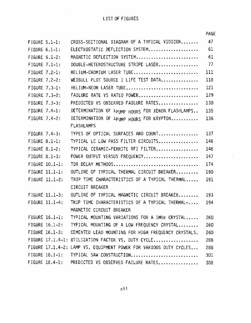
LIST OF FIGURES
PAGE
FIGURE 5.1-1: CROSS-SECTIONAL DIAGRAM OF A TYPICAL VIDICON 47
FIGURE 6.1-1: ELECTROSTATIC DEFLECTION SYSTEM 61
FIGURE 6.1-2: MAGNETIC DEFLECTION SYSTEM 61
FIGURE 7.1-1: DOUBLE-HETEROSTRUCTURE STRIPE LASER 77
FIGURE 7.2-1: HELIUM-CADMIUM LASER TUBE Ill
FIGURE 7.2-2: WEIBULL PLOT SOURCE 1 LIFE TEST DATA 118
FIGURE 7.3-1: HELIUM-NEON LASER TUBE 121
FIGURE 7.3-2: FAILURE RATE VS RATED POWER 129
FIGURE 7.3-3: PREDICTED VS OBSERVED FAILURE RATES 130
FIGURE 7.4-1: DETERMINATION OF X P U M P HOURS FOR XENON FLASHLAMPS.. 135
FIGURE 7.4-2: DETERMINATION OF XpUMp HOURS FOR KRYPTON 136
FLASHLAMPS
FIGURE 7.4-3: TYPES OF OPTICAL SURFACES AND COUNT 137
FIGURE 8.1-1: TYPICAL LC LOW PASS FILTER CIRCUITS 146
FIGURE 8.1-2: TYPICAL CERAMIC-FERRITE RFI FILTER 146
FIGURE 8.1-3: POWER OUTPUT VERSUS FREQUENCY 147
FIGURE 10.1-1: TDR DELAY METHODS 174
FIGURE 11.1-1: OUTLINE OF TYPICAL THERMAL CIRCUIT BREAKER 190
FIGURE 11.1-2: TRIP TIME CHARACTERISTICS OF A TYPICAL THERMAL 191
CIRCUIT BREAKER
FIGURE 11.1-3: OUTLINE OF TYPICAL MAGNETIC CIRCUIT BREAKER 193
FIGURE 11.1-4: TRIP TIME CHARACTERISTICS OF A TYPICAL THERMAL-.... 194
MAGNETIC CIRCUIT BREAKER
FIGURE 16.1-1: TYPICAL MOUNTING VARIATIONS FOR A 1MHz CRYSTAL 260
FIGURE 16.1-2: TYPICAL MOUNTING OF A LOW FREQUENCY CRYSTAL 260
FIGURE 16.1-3: CEMENTED LEAD MOUNTING FOR HIGH FREQUENCY CRYSTALS. 260
FIGURE 17.1.4-1: UTILIZATION FACTOR VS. DUTY CYCLE 288
FIGURE 17.1.4-2: LAMP VS. EQUIPMENT POWER FOR VARIOUS DUTY CYCLES... 288
FIGURE 18.1-1: TYPICAL SAW CONSTRUCTION 301
FIGURE 18.4-1: PREDICTED VS OBSERVED FAILURE RATES 308
xii

LIST OF TABLES
PAGE
TABLE 2.2-1: DATA SUMMARY BY DEVICE 7
TABLE 3.1-1: EXAMPLE OF QUALITATIVE REGRESSION ANALYSIS 10
TABLE 3.3-1: ENVIRONMENTAL STRESS RATIOS 25
TABLE 3.3-2: ENVIRONMENTAL FACTOR DEVELOPMENT 27
TABLE 4.3-1: UTILIZATION FACTOR 32
TABLE 4.3-2: ENVIRONMENTAL FACTOR 33
TABLE 4.4-1: MAGNETRON FAILURE RATE DATA 34
TABLE 4.4-2: MAGNETRON CONSTRUCTION AND APPLICATION VARIABLES... 36
TABLE 4.4-3: MAGNETRON VARIABLE IDENTIFICATION 39
TABLE 4.4-4: RESULTS OF THE REGRESSION ANALYSIS 40
TABLE 4.4-5: OBSERVED MAGNETRON ENVIRONMENTAL FACTORS 42
TABLE 4.4-6: ENVIRONMENTAL FACTOR COMPARISONS 44
TABLE 5.3-1: ENVIRONMENTAL FACTORS 53
TABLE 5.4-1: VIDICON FAILURE RATE DATA 54
TABLE 5.4-2: VIDICON CONSTRUCTION AND APPLICATION VARIABLES 55
TABLE 5.4-3: NORMALIZED FAILURE RATES 56
TABLE 6.3-1: ENVIRONMENTAL MODE FACTORS 66
TABLE 6.3-2: LEARNING FACTOR 66
TABLE 6.4-1: CRT FIELD EXPERIENCE DATA 67
TABLE 6.4-2: CRT CONSTRUCTION AND APPLICATION VARIABLES 68
TABLE 6.4-3: RESULTS OF CRT REGRESSION ANALYSIS 69
TABLE 6.4-4: AiC ENVIRONMENTAL FACTOR CONFIDENCE INTERVALS 70
TABLE 7.0-1: LASER CONSTRUCTION AND APPLICATION VARIABLES 73
TABLE 7.1-1: SSO DISTRIBUTION 85
TABLE 7.1-2: ENVIRONMENTAL MODE FACTORS 89
TABLE 7.1-3: DEGRADATION EQUATION PARAMETERS 89
TABLE 7.1-4: CONSTRUCTION FACTORS 89
TABLE 7.1-5: APPLICATION FACTOR 89
TABLE 7.1-6: PULSED DUTY CYCLE FACTOR 89
TABLE 7.1-7: TEMPERATURE AND CURRENT LIMITS 90
TABLE 7.1-8: TEST DATA 92
xiii

LIST OF TABLES (CONT'D)
PAGE
TABLE 7.1-9: CONSTRUCTION FACTORS 95
TABLE 7.1-10: DUTY CYCLE DEGRADATION RATES 96
TABLE 7.1-11: ASSUMED DUTY CYCLE FACTORS 96
TABLE 7.1-12: APPLICATION FACTORS 97
TABLE 7.1-13: LASER CATEGORIES 98
TABLE 7.1-1 : SSO DISTRIBUTION 100
TABLE 7.1-15: FUNCTIONAL DEGRADATION MODE DISTRIBUTION 101
TABLE 7.1-16: MODEL CONSTANTS 103
TABLE 7.1-17: WEIBULL AND LOGNORMAL PARAMETERS COMPARISONS 106
TABLE 7.1-18: K-S TEST RESULTS 106
TABLE 7.2-1: HELIUM-CADMIUM FAILURE MECHANISM DISTRIBUTION 113
TABLE 7.2-2: ENVIRONMENTAL MODE FACTORS 115
TABLE 7.2-3: LIFE TEST TIME-TO-FAILURE 116
TABLE 7.2-4: EMPIRICAL FAILURE DATA 117
TABLE 7.2-5: NORMALIZED FAILURE RATES 120
TABLE 7.2-6: PREDICTED/OBSERVED FAILURE RATES .... 120
TABLE 7.3-1: ENVIRONMENTAL MODE FACTORS 123
TABLE 7.3-2: HELIUM-NEON LASER DATA , 125
TABLE 7.3-3: NORMALIZED-MERGED DATA 126
TABLE 7.3-4: HOMOGENEITY TEST 126
TABLE 7.3-5: DATA MERGED BY TUBE RATED POWER 127
TABLE 7.3-6: REVISED X m e d i a ESTIMATE 128
TABLE 7.4-1: SSR ENVIRONMENTAL FACTORS 134
TABLE 7.4-2: COUPLING CLEANLINESS FACTORS 134
TABLE 7.4-3: Nd:YAG FAILURE EXPERIENCE DATA 139
TABLE 7.4-4: Nd:YAG PREDICTIONS 140
TABLE 7.4-5: PREDICTED AND OBSERVED FAILURE RATES 141
TABLE 7.4-6: SIMMER CIRCUIT ANALYSIS 142
TABLE 8.1-1: EXAMPLES OF FILTER CONSTRUCTION 148
TABLE 8.2-1: FILTER FAILURE MODES 149
TABLE 8.3-1: ENVIRONMENTAL FACTORS 151
xiv

LIST OF TABLES (CONT'D)
PAGE
TABLE 8.4-1: FILTER FIELD EXPERIENCE DATA 153
TABLE 8.4-2: FILTER CONSTRUCTION AND APPLICATION VARIABLES 155
TABLE 8.4-3: RESULTS OF FILTER REGRESSION ANALYSIS 157
TABLE 8.4-4: RESULTS OF FILTER REGRESSION ANALYSIS 158
TABLE 9.3-1: SSR ENVIRONMENTAL FACTORS 164
TABLE 9.4-1: SSR FAILURE EXPERIENCE DATA 166
TABLE 9.4-2: SSR ENVIRONMENT FACTOR INFORMATION 167
TABLE 9.4-3: SSR REGRESSION ANALYSIS RESULTS 168
TABLE 10.1-1: TDR PART COUNT 175
TABLE 10.2-1: TDR FAILURE MODES/OPERATING CHARACTERISTICS AND.... 176
EFFECTS
TABLE 10.3-1: ENVIRONMENTAL FACTORS 179
TABLE 10.4-1: TDR FIELD EXPERIENCE DATA 181
TABLE 10.4-2: PREDICTED AND OBSERVED FAILURE RATES 183
TABLE 10.4-3: TDR ENVIRONMENT FACTOR INFORMATION 185
TABLE 10.4-4: TDR REGRESSION ANALYSIS RESULTS 186
TABLE 11.2-1: CIRCUIT BREAKER FAILURE MODE DISTRIBUTION 195
TABLE 11.3-1: CONFIGURATION FACTOR 198
TABLE 11.3-2:. ENVIRONMENTAL FACTOR 199
TABLE 11.4-1: CIRCUIT BREAKER FAILURE RATE DATA.. 201
TABLE 11.4-2: CIRCUIT BREAKER CONSTRUCTION AND APPLICATION 202
VARIABLES
TABLE 11.4-3: RESULTS OF CIRCUIT BREAKER REGRESSION ANALYSIS 204
TABLE 11.4-4: CONFIDENCE INTERVALS FOR CIRCUIT BREAKERS 204
PARAMETERS
TABLE 11.4-5: CONFIGURATION FACTOR ANALYSIS 205
TABLE 11.4-6: ENVIRONMENTAL FACTORS OF ELECTROMECHANICAL PARTS... 206
TABLE 11.4-7: CIRCUIT BREAKER FAILURE RATE DATA MERGED BY 207
ENVIRONMENT
TABLE 11.4-8: CHI-SQUARED TEST TO DETERMINE OPTIMAL 208
ENVIRONMENTAL FACTORS
XV
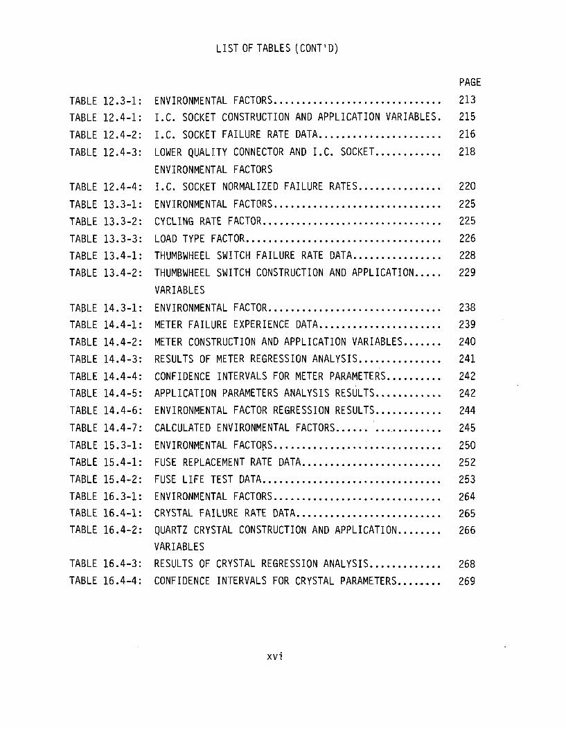
LIST OF TABLES (CONT'D)
PAGE
TABLE 12.3-1: ENVIRONMENTAL FACTORS 213
TABLE 12.4-1: I.C. SOCKET CONSTRUCTION AND APPLICATION VARIABLES. 215
TABLE 12.4-2: I.C. SOCKET FAILURE RATE DATA 216
TABLE 12.4-3: LOWER QUALITY CONNECTOR AND I.C. SOCKET 218
ENVIRONMENTAL FACTORS
TABLE 12.4-4: I.C. SOCKET NORMALIZED FAILURE RATES 220
TABLE 13.3-1: ENVIRONMENTAL FACTORS 225
TABLE 13.3-2: CYCLING RATE FACTOR 225
TABLE 13.3-3: LOAD TYPE FACTOR 226
TABLE 13.4-1: THUMBWHEEL SWITCH FAILURE RATE DATA 228
TABLE 13.4-2: THUMBWHEEL SWITCH CONSTRUCTION AND APPLICATION 229
VARIABLES
TABLE 14.3-1: ENVIRONMENTAL FACTOR 238
TABLE 14.4-1: METER FAILURE EXPERIENCE DATA 239
TABLE 14.4-2: METER CONSTRUCTION AND APPLICATION VARIABLES 240
TABLE 14.4-3: RESULTS OF METER REGRESSION ANALYSIS 241
TABLE 14.4-4: CONFIDENCE INTERVALS FOR METER PARAMETERS 242
TABLE 14.4-5: APPLICATION PARAMETERS ANALYSIS RESULTS 242
TABLE 14.4-6: ENVIRONMENTAL FACTOR REGRESSION RESULTS 244
TABLE 14.4-7: CALCULATED ENVIRONMENTAL FACTORS 245
TABLE 15.3-1: ENVIRONMENTAL FACTORS 250
TABLE 15.4-1: FUSE REPLACEMENT RATE DATA 252
TABLE 15.4-2: FUSE LIFE TEST DATA 253
TABLE 16.3-1: ENVIRONMENTAL FACTORS 264
TABLE 16.4-1: CRYSTAL FAILURE RATE DATA 265
TABLE 16.4-2: QUARTZ CRYSTAL CONSTRUCTION AND APPLICATION 266
VARIABLES
TABLE 16.4-3: RESULTS OF CRYSTAL REGRESSION ANALYSIS 268
TABLE 16.4-4: CONFIDENCE INTERVALS FOR CRYSTAL PARAMETERS 269
xvi

LIST OF TABLES (CONT'D)
PAGE
TABLE 17.1.3-1: UTILIZATION FACTOR 275
TABLE 17.1.3-2: ENVIRONMENTAL FACTOR 276
TABLE 17.1.4-1: INCANDESCENT LAMP FAILURE RATE DATA 277
TABLE 17.1.4-2: INCANDESCENT LAMP CONSTRUCTION AND APPLICATION.... 278
VARIABLES
TABLE 17.1.4-3: INCANDESCENT LAMP VARIABLE IDENTIFICATION 281
TABLE 17.1.4-4: RESULTS OF THE REGRESSION ANALYSIS 281
TABLE 17.1.4-5: INTERIM UTILIZATION FACTOR 289
TABLE 17.1.4-6: UTILIZATION FACTOR 290
TABLE 17.2-1: GLOW LAMP CONSTRUCTION AND APPLICATION VARIABLES.. 297
TABLE 17.2-2: GLOW LAMP FAILURE EXPERIENCE DATA 298
TABLE 18.2-1: REPORTED FAILURE MODES/MECHANISMS 303
TABLE 18.3-1: ENVIRONMENTAL FACTORS 304
TABLE 18.4-1: SAW FAILURE EXPERIENCE DATA 305
TABLE 18.4-2: ENVIRONMENTAL COMPARISONS 306
TABLE 18.4-3: NORMALIZED FAILURE DATA 306
xvii

1.0 INTRODUCTION
1.1 Objective
The objective of this study effort was to develop failure rate prediction
models for the following thermionic, coherent light emitting, passive and
electromechanical devices:
o Magnetrons (including low power C.W.)
o Vidicons
o Cathode Ray Tubes
o Lasers
o Electronic Filters
o Solid State Relays
o Electronic Time Delay Relays
o Circuit Breakers
o I.C. Sockets
o Thumbwheel Switches
o Electromagnetic Meters
o Fuses
o Crystals
o Incandescent Lamps
o Glow Lamps
o Surface Acoustic Wave Devices
The derived prediction methodologies are intended to provide the ability to
predict the total device reliability as a function of the characteristics of
the device, the technology employed in producing the device, and those
external factors, e.g., environmental stresses, circuit application, etc.
which have a significant affect on device reliability. The prediction
methodology was formatted in a form compatible with MIL-HDBK-217.
1

1.2 Background
Failure rate and mean-time-between-failure prediction capabilities are
essential tools in the development and maintenance of reliable electronic
equipments. Predictions performed during the design phase yield early
estimates of the anticipated equipment reliability and provide a
quantitative basis for performing proposal evaluations, design trade-off
analyses, reliability growth monitoring and life-cycle cost studies. While
the majority of the device models in MIL-HDBK-217 afford reasonably accurate
predictions, the same cannot be said for the devices enumerated in Section
1.1. Vidicons, electronic filters, solid state relays, I.C. sockets and
surface acoustic wave devices are not represented by a model, while the
models for the remaining devices are inadequate or may have become obsolete
as a consequence of advancing technology.
1.3 Modeling Approach
The general approach used for the development of viable prediction
methodologies for these critical electronic devices is described in this
section.
Critical factors which were thought to ultimately impact the reliability
of a device were identified for each critical device. These factors which
were considered in detail included:
o Function
o Technology
Fabrication Techniques
Fabrication Process Maturity
Failure Mode/Mechanism Experience
o Complexity
o Effectiveness of Process Controls
o Effectiveness of Screening and Test Techniques
o Operating Temperature and Environment
o Application Considerations
2
The information required to identify these factors was obtained from the
shared experiences of the personnel working on the study (IITRI corporate
memory) and from the literature search discussed in Section 2.1.
A model form was hypothesized based on information obtained from IITRI' s
corporate memory and from the literature search discussed in Section 2.1.
Data obtained from the data collection effort discussed in Section 2.2 were
analyzed to evaluate the accuracy of the hypothesized model form and to
generate numerical estimates for the parameters included in the model.
Field failure experience data were utilized where ever possible. In some
instances insufficient field experience data were available, and either life
test data and/or physics of failure information and/or the present
relationships between factors in the current MIL-HDBK-217 models were used
to derive numerical estimates for the parameters included in the proposed
model.
A detailed discussion of the modeling approach used to develop each model
is presented in the model development section for each model.
1.4 Report Organization
This technical report is organized as follows:
Section 1.0 - A general introduction concerning the objective of the study, the rationale for the study and the basic modeling approach used.
Section 2.0 - A general discussion of the data collection and literature search(s) employed.
Section 3.0 - A general discussion of the statistical procedures used in the data analyses and model development
Section 4.0 - Detailed discussions of the applicable part descrip-thru tions, part failure modes/mechanisms, proposed model, Section 18.0 model development approach, references and
bibliography.
3

Section 19.0 - Conclusion and recommendations.
Appendix A - Revision pages for MIL-HDBK-217.

2.0 DATA/INFORMATION COLLECTION TECHNIQUES
2.1 Literature Review
A comprehensive literature review was performed for each device type
considered in the study. The purpose of the review was to identify all
published information which was thought to be relevant to the reliability of
the critical devices. Literature sources searched included the Reliability
Analysis Center a* tomated library information retrieval system, the National
Technical Information Service (NTIS), the Defense Technical Information
System (DTIS), the Government Industry Data Exchange Program (GIDEP), the
RADC Technical Library and the John Crerar library. Additionally,
manufacturers and users of the devices were queried to supply useful
information.
The primary objective of the literature review was to locate references
whose content could be used to define relevant device characteristics and to
hypothesize a model form, to supplement the data analysis process and to
provide the reliability models with a sound theoretical foundation.
The information sources that were identified and utilized in the study
are presented in the appropriate section.
2.2 Data Collection and Preliminary Analysis
The modification of current failure rate prediction models or the
development of new prediction methodologies should be derived from field
failure rate data obtained from monitored systems. This section presents the
basic data collection procedure followed and the preliminary analyses used
to develop useful databases for the devices.
The Reliability Analysis Center operated by the IIT Research Institute
at Griffiss Air Force Base was solicited to aid in the data collection
process. The Reliability Analysis Center regularly pursues the collection of
parts reliability data including those devices to be analyzed in this study.
5

Data resources which had been collected and summarized prior to the
initiation of this study were available for analysis. However, the
requirements for extensive data resources necessitated additional data
collection activities to supplement the existing information.
A survey of commercial, industrial and government organizations was
conducted shortly after the beginning of the study. Organizations contacted
either manufactured, used or were similarly connected with one or more of the
devices considered in this study. Information requested included field
experience data, pre-production and production equipment tests, failure
analysis reports and physical construction details. A sum total of over 787
organizations were contacted. Approximately 15% of all organizations
contacted during the data collection effort submitted information pertaining
to one or more of the critical electronic devices. A primary concern of the
majority of contributors was the proprietary nature of the information and
the desire to remain anonymous. For this reason, none of the data
contributors in this study will be identified.
A prerequisite to the summarization of data was the identification of all
parameters and factors influencing the reliability of the devices. A task
was defined at the beginning of the program whose goal was a reliability
evaluation based solely on theoretical considerations. These theoretical
studies served to identify the important parameters which were then further
investigated using data analysis. Identification of construction details
and process controls which were theoretically believed to have an effect on
reliability were pursued for each source of data.
All data items received during the data collection efforts were reviewed
for completeness of detail and examined for any inherent biases. Any data
submittal which displayed obvious biases were not considered in this study.
Those reports lacking sufficient detail were not considered until the
necessary additional information was acquired.
A summary of the collected and reduced data is given in Table 2.2-1.
Table 2.2-1 presents part operating hours and recorded failures for each
6

device type. A detailed list of the data collected on each device type is
presented in the appropriate section.
TABLE 2.2-1: DATA SUMMARY BY DEVICE
Device Device Number of Operate Hours Failures
(X 10&)
Magnetrons
Vidicons
Cathode Ray Tubes
Semiconductor Lasers
Helium-Cadmium Lasers
Helium-Neon Lasers
Nd:YAG Lasers
Electronic Filters
Solid State Relays
Time Delay Relays
Circuit Breakers
I.C. Sockets
Thumbwheel Switches
Meters
Fuses
Crystals
Incandescent Lamps
Neon Lamps
Surface Acoustic Wave Devices
Totals
6.941
29.132
5.079
4.051
0.358
4.708
0.176
580.955
23853.760
4.012
334.198
3478.129
5.485
60.799
800.401
' 44.469
213.433
60.877
1.577
29488.540
1950
482
91
354
90
25
25
73
702
6
379
2
18
108
185
16
893
27
2
5428
Notes: (1) includes both failures and replacements
7
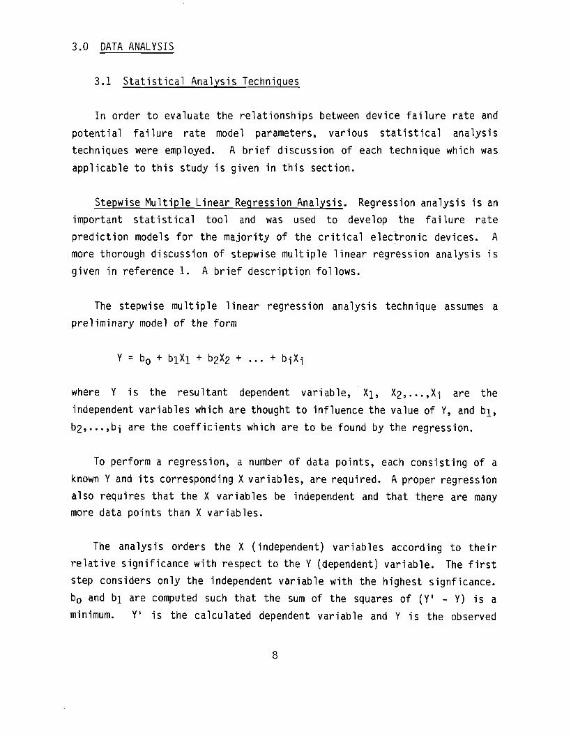
3.0 DATA ANALYSIS
3.1 Statistical Analysis Techniques
In order to evaluate the relationships between device failure rate and
potential failure rate model parameters, various statistical analysis
techniques were employed. A brief discussion of each technique which was
applicable to this study is given in this section.
Stepwise Multiple Linear Regression Analysis. Regression analysis is an
important statistical tool and was used to develop the failure rate
prediction models for the majority of the critical electronic devices. A
more thorough discussion of stepwise multiple linear regression analysis is
given in reference 1. A brief description follows.
The stepwise multiple linear regression analysis technique assumes a
preliminary model of the form
Y = b 0 + biXi + b2X2 + ... + b -,- X -j
where Y is the resultant dependent variable, Xi, X2,...,X-j are the
independent variables which are thought to influence the value of Y, and b]_,
b 2»• - •»b -j are the coefficients which are to be found by the regression.
To perform a regression, a number of data points, each consisting of a
known Y and its corresponding X variables, are required. A proper regression
also requires that the X variables be independent and that there are many
more data points than X variables.
The analysis orders the X (independent) variables according to their
relative significance with respect to the Y (dependent) variable. The first
step considers only the independent variable with the highest signficance.
b 0 and bi are computed such that the sum of the squares of (Y1 - Y) is a
minimum. Y' is the calculated dependent variable and Y is the observed
8
dependent variable. The second X variable is then considered and b0, bi and
b2 are computed such that the sum of the sqares of (Y1 - Y) is again a
minimum. If the improvement in the estimate afforded by the inclusion of
this second variable is significant with respect to a given confidence level,
the variable is accepted as part of the model. If considering the second
variable does not result in a significant improvement the model remains,
Y = b 0 + biXi
In the case where the second variable is accepted, the regression
analysis continues until all of the significant X variables have been
identified and the corresponding bn- coefficients have been calculated.
However, whenever a new variable is included in the fitted model, all
previously included variables are retested for significance and eliminated
if insignificant.
Failure rate prediction models are rarely in the additive form the
stepwise linear regression analysis assumes. However, by using
transformations, many possible model forms can assume the additive form. An
example can best illustrate this point. • The Arrhenius relationship is
applicable to many electrical devices and takes the following form,
X = A exp (-B/T)
where T is the independent variable, *• is the dependent variable and A and B
are constants. By taking the logarithm of each side the equation becomes,
lnX = InA - Y
which can be solved by regression analysis with 1/T the independent variable
and lnX i-'ne dependent variable. Other transformations are available such
that stepwise multiple linear regression can be used to quantify a variety of
failure rate model forms.
9
The previous paragraphs have discussed how regression analysis can be
useful in developing failure rate prediction models in which failure rate is
a function of quantitative variables such as temperature, frequency or peak
power level. However, there are often significant variables which can not be
measured on a continuous quantitative scale. Application environment and
manufacturing quality level are examples of variables which are qualitative.
Numerically it is difficult to relate "ground benign" environmental stress
to "airborne inhabited fighter" environmental stress although one is known
to be worse than the other. In order to determine numerical quantities for
qualitative factors in a regression analysis, a matrix of "dummy variables"
(0 or 1) is used as the independent variables. The regression solution by
least squares gives numerical values of the coefficients (b-j) which can be
used to calculate numerical quantities corresponding to the appropriate
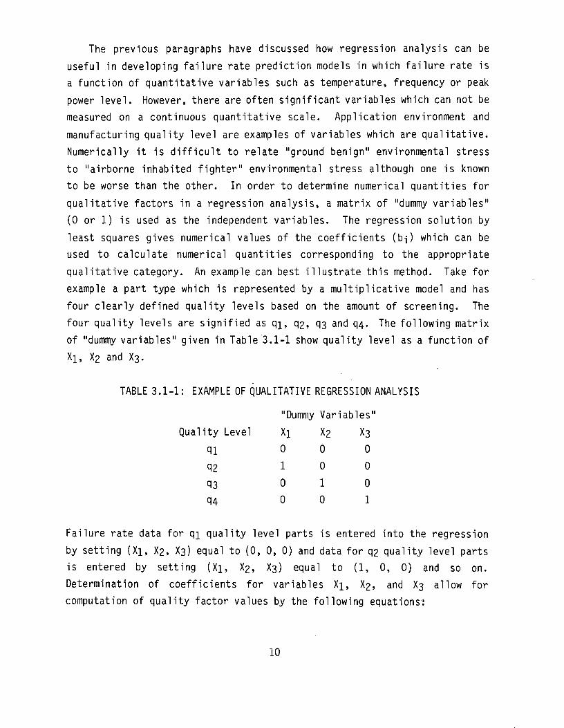
qualitative category. An example can best illustrate this method. Take for
example a part type which is represented by a multiplicative model and has
four clearly defined quality levels based on the amount of screening. The
four quality levels are signified as q]_, q2, q3 and q4. The following matrix
of "dummy variables" given in Table 3.1-1 show quality level as a function of
Xi, X2 and X3.
TABLE 3.1-1: EXAMPLE OF QUALITATIVE REGRESSION ANALYSIS
Quality
qi
q2
q3 q4
Level
"Dummy
Xl 0
1
0 0
Variables
X2 X3
0 0
0 0
1 0
0 1
Failure rate data for q\ quality level parts is entered into the regression
by setting (Xi, X2, X3) equal to (0, 0, 0) and data for q2 quality level parts
is entered by setting (Xi, X2, X3) equal to (1, 0, 0) and so on.
Determination of coefficients for variables Xi, X2, and X3 allow for
computation of quality factor values by the following equations?
10
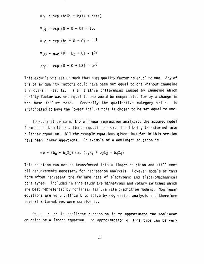
TTQ = exp (biXi + b2X2 + b3X3)
TTQI = exp (0 + 0 + 0) = 1.0
TTQ2 = exp (bi + 0 + 0) = e b l
TTQ3 = exp (0 + b2 + 0) = e b 2
TTQ4 = exp (0 + 0 + b3) = e b 3
This example was set up such that a qi quality factor is equal to one. Any of
the other quality factors could have been set equal to one without changing
the overall results. The relative differences caused by changing which
quality factor was set equal to one would be compensated for by a change in
the base failure rate. Generally the qualitative category which is
anticipated to have the lowest failure rate is chosen to be set equal to one.
To apply stepwise multiple linear regression analysis, the assumed model
form should be either a linear equation or capable of being transformed into
a linear equation. All the example equations given thus far in this section
have been linear equations. An example of a nonlinear equation is,
Xp = (b0 + biXi) exp (b2X2 + b3X3 + b4X4)
This equation can not be transformed into a linear equation and still meet
all requirements necessary for regression analysis. However models of this
form often represent the failure rate of electronic and electromechanical
part types. Included in this study are magnetrons and rotary switches which
are best represented by nonlinear failure rate prediction models. Nonlinear
equations are very difficult to solve by regression analysis and therefore
several alternatives were considered.
One approach to nonlinear regression is to approximate the nonlinear
equation by a linear equation. An approximation of this type can be very
11

accurate as long as there are clearly defined minimum and maximum values for
the independent variables which are part of the approximation. This approach
was used for magnetrons. The assumed form for magnetron failure rate with
and without the approximation are given below.
Xp = Xb (Ar + B) fc Pd T E , empirical model form
^p = ^b U r b ) fc p<^ ^E » model form with approximation
where r, f and P are independent variables and X b j A, B, a, b, c and d are
constants. All factors are clearly defined in Section 4.3. r is a ratio
which can vary from 0 to 1. The approximation proved to be very accurate for
r values from 0.2 to 1.
Another approach to nonlinear regression is to transform the assumed
equation form such that the right hand side of the equation (independent
variables and coefficients) is linear. The resulting left hand side of the
equation is treated as the dependent variable. This approach does not
strictly adhere to the theoretical requirements necessary for application of
stepwise multiple linear regression analysis. However, this is often done in
reliability modeling efforts and errors caused by this transformation are
minimal if applied carefully. An example would be normalizing the failure
rate for environment before applying regression. Another example is the
rotary switch failure rate prediction model which is given by the following
equation:
X p = (X]_ + X 2 N) TTE TTcyc TTL
where N is an independent variable, X p is the dependent variable, Xi and X 2
are constants and TTE, ^CyC and T ^ are modifying factors which were assumed
correct for all types of rotary switches. In order to apply regression
analysis so that X^ and X 2 can be determined, the equation is transformed (or
normalized) to the following form,
12

Xp/(TTE *cyc vl) = h + x 2 ^
If the entire left hand side of this equation is treated as the dependent
variable, then the equation becomes linear and regression can be applied.
F Ratio and Critical F. The F Ratio and Critical F are statistical
parameters which are used in conjunction with regression analysis to
determine significance of independent variables. The Critical F value is the
value from the F table given in Reference 1) corresponding to the degrees of
freedom of the model (equal to the number of data points minus the number of
b-j coefficients minus one). This number may be used to test the significance
of each variable as it is considered for addition to or deletion from the
model. The F ratio value for a regression is the quotient of the mean square
due to regression and the mean square due to residual variation. If the F
Ratio value for any independent variable is greater than the critical F
value, then it is considered a significant factor influencing failure rate
and is included in the regression analysis model.
Standard Error of Estimate. The standard error of estimate gives ;:n
indication of the confidence of an individual b-j coefficient determined from
a regression analysis. The standard error is equal to the square root of the
residual mean square (the estimate of the variance about the regression).
Upper and lower confidence limits of the regression coefficients can be
determined from the standard error and are given for a predetermined
confidence (a) by,
tM + tn_2 (S.E.)
where
b-j = regression coefficient
tn_2 = 1 - h a percentage point of a t - distribution with n-2 degrees of freedom
n = number of observations
13

S.E. = standard error of estimate
When the assumed failure rate model form is a multiplicative model, the upper
and lower confidence limit values are not exact but are approximate due to
the transformation. Values for the t - distribution are given in Reference
1.
Multiple Coefficient of Determination. The multiple coefficient of
determination is equal to the ratio of the sum of squares of the variance
explained by the regression to the sum of the squares of the variance of the
observed data. The correlation coefficient is often used as a means to
select the optimal form of a failure rate prediction model (i.e. linear,
exponential). The coefficient ranges from 0 to 1.0. A coefficient value of
1.0 indicates a perfect fit between the model and observed data.
The Correlation Coefficient. The correlation coefficient is a measure
of the relation between any two variables. It varies between -1 and 1 (from
perfect negative to perfect positive correlation).
Chi-Squared Goodness of Fit Test. The chi-squared goodness of fit test
compares observed data to expected values to determine whether the data is
representative of the hypothesized distribution. The chi-squared statistic
is given by the following equation.
y2 = £ (o-e)2
e
where
X^ = chi-squared value
o = observed value
e = predicted value
The chi-squared statistic indicates whether the observed events differ from
predicted values at a set level of significance for a given degrees of
14

freedom. Relatively lower chi-squared values indicate a better fit between
observed data and predicted values. Chi-squared tables are given in
Reference 2.
Chi-squared Confidence Intervals. The chi-squared statistic is used to
identify a confidence interval around the failure rate point estimate for an
exponentially distributed failure rate. For example the 90% confidence
interval is comprised of the lower 5% confidence and upper 95% confidence
limit values. A 90% confidence interval is the range of values around the
point estimate that would, with a 90% probability, include the mean of an
infinite sample of similar devices. Assumptions concerning data censoring
are made in order to calculate the confidence interval values. These values
are calculated as follows:
Y2 (]_ a ?r) Lower Confidence Limit = A—o^r-2
Point estimate = j
Upper Confidence Limit
where
r = numer of failures
T = total part hours
X^(a) = Chi-squared value corresponding to-a particular confidence level
and degrees of freedom (obtained from Chi-square tables, given
in Reference 2)
Kolmoqorov-Smirnov Goodness of Fit Test. This test performs essentially
the same function as the chi-squared test. It is also a non-parametric test
which indicates the goodness of fit by analyzing the maximum difference
between observed and predicted values for a theoretical cumulative
distribution. If the maximum difference is larger than a preselected
critical value for a given level of significance, then the observed events
_ y? (1-a. 2r + 2) 2T
15

would not appear to follow the assumed theoretical distribution. The
Kolmogorov-Smirnov test is generally used when testing the goodness of fit of
a Weibull distribution. A more thorough description and K-S critical value
tables are given in reference 2.
Homogeneity Test for Merging Data. A computerized program developed by
IITRI was utilized to determine whether failure rate data from diverse
sources can be merged. This method is presented in detail in Reference 3. A
brief description of this test is presented in this section.
Given data of the form,
r*i failures in time t\
V2 failures in time t2
etc.
mean time between failure (MTBF) can be computed for each data record and an
observed histogram of frequency of occurence vs. MTBF can be determined. The
computerized program then uses Monte Carlo simulation to hypothesize a
theoretical distribution of MTBF. If all data records are from the same
underlying distribution, then the observed and simulated distributions
should be in agreement. If the simulated deviates significantly from the
observed distribution, then some nonhomogeneity is indicated. The
Kolmogorov-Smirnov goodness of fit test is used as the relative measure of
whether the observed and simulated distributions are in agreement and the
data can be merged. Several reasons for failure rate data not merging are
the existance of outliers which can be natural or due to poor data collection
practices, or that the data records are not similar in regard to all
significant variables effecting failure rate.
The statistical techniques described in this section represent useful
tools applicable to reliability modeling efforts. It must be emphasized,
however, that all reliability prediction models derived in this study are
16
based on a sound theoretical basis. The statistical techniques are most
useful as a complement to engineering analyses and not as a substitute.
3.2 Data Deficiencies and Data Quality Control
Reliability modeling of electronic or electromechanical components
ideally requires a large database of failure rate data available for
analysis. The part types considered in this study effort can be classified
as low population or low usage parts. Therefore, development of failure rate
databases which are both plentiful and accurate, is difficult, if not
impossible. This section presents a brief overview of inherent problems with
available data and data quality control measures implemented to insure
accurate failure rate prediction models.
Available sources of failure rate data are generally either life test
data supplied from part manufacturers or equipment level field experience
data. Each type of data has several inherent difficulties.
Life test data generally are of a high statistical quality because there
is \iery little uncertainty with regard to recorded failures, number of parts
on test, test time, operating conditions and environmental conditions.
However, caution must be applied when using this type of data for reliability
modeling efforts. Often the life test conditions are at an elevated
temperature or voltage to accelerate the frequency of observed failures.
Extrapolation of failure rates obtained at the accelerated conditions to
more normal operating conditions may introduce error, if extrapolation is
possible at all. Another problem associated with life test data obtained
from part manufacturers is one of validity. The majority of part
manufacturers are unquestionably honest. However, the question arises as to
whether the data which is supplied is representative of all life testing
performed.
Several measures were implemented to minimize the detrimental effects of
using life test data. First, for part types where field experience data was
17

available, life test data was only used to complement field experience data.
Second, only life test data with operating and temperature conditions which
are typical of a ground, benign environment were used in regression analyses
in conjunction with field experience data. The proposed failure rate
prediction model for semiconductor lasers was the only model presented in
this report which was based primarily on life test data.
Field experience data are the more desirable type of data since they
represent what actually occurred in the field and this is what the proposed
model attempts to predict. The inherent difficulties with field experience
data are related to the accuracy with which a failure can be defined, the
precision with which the number of part hours can be measured, and the
ability to determine the stresses applied to a part.
A problem associated with all sources of field experience data is that
individual times to failure can not be determined. Data is available in the
form of R failures observed in T part hours. The part hours represent a
cumulative count of part hours from individual components. The result of
this data deficiency is that the exponential hazard rate function must be
applied to all part types. For most electronic parts it has been documented
that this assumption does not introduce significant error. For
electromechanical parts and other part types where degradation failure
mechanisms are significant, the constant failure rate calculated by dividing
the observed failures by the recorded part hours represents the random
failure rate plus an average degradation failure rate contribution.
The best sources of field experience data are from military systems where
the number of observed failures and equipment operating hours are precisely
recorded because of contractual agreements. Examples of government
contracts which require monitoring of failures and part hours are
Reliability Improvement Warrenty (RIW) and Life-Cycle Cost (LCC) contracts.
Specific military equipments of this type which were utilized in this study
effort are the AN/ARN-118 TACAN radio set, the AN/UYK-7 Navy computer and
18
the AN/ARC-164 radio set. Unfortunately there are relatively few military
equipments of this type.
A more plentiful source of failure rate data for fielded military
equipments are maintenance data systems maintained by the different branches
of the armed forces. The largest of these are the AFM66-1 system maintained
by the U.S. Air Force, the 3M system maintained by the U.S. Navy and the
Sample Data Collection system maintained by the U.S. Army, TSARCOM. These
systems are designed to provide equipment-level statistics such as
availability and equipment mean time between failures. Some also provide
information on failed components in order to assist in spares provisioning
and logistics support. None of these systems is intended to track
reliability to the piece-part level. It has been found, however, that this
can be done with some degree of accuracy by using the failure records from
one of the maintenance data systems.
There are several major problems associated with using one of the
maintenance data systems as a source of part level failure rate data. The
major problem is that the data provides the analyst with the number of part
replacements and not the number of part failures. It is very difficult to
separate true failures from part replacements which were secondary failures
or which were due to operator error, maintenance error or other factors.
Several measures can be taken to minimize the difference between
"replacements" and "failures". First, data should only be collected on part
types where the ratio of replacement rate to failure rate is known to be low.
Maintenence technicians often replace many board mounted components such as
resistors before finding the actual failed component. Second, caution
should be applied when collecting data on part types which are easily
replaced and the replacement possibly not recorded. Parts of this type are
incandescent lamps and fuses. Third, other codes included in the maintenance
data summaries such as "action taken" code, "when discovered" code, "type
maintenance" code and "how malfunctioned" code must be analyzed. Failures
which occur during periods of nonoperation, or part replacements which are
due to operator or maintenance error can often be identified by analyzing
19

these codes. The U.S. Army Sample Data Collection system maintained by
TSARCOM, St. Louis, MO includes a chargeability code to denote whether part
replacements are true failures for the ground transportable generator sets
which they collect data on. This is an encouraging development and if
implemented on a broad scale, it would increase the accuracy of data
collected from maintenance data collection systems.
Field failure experience data samples for most electronic and
electromechanical parts are necessarily restricted because the average mean
time to failure (approximately 10^ to 10? part hours) is, in many cases, much
longer than the technology has been available. However good the failure rate
data, it can only cover the first few percentiles of the probability density
function. One result of these relatively high mean time to failures for most
part types is the presence of data records with zero observed failures.
For "zero failure" data records, the standard method of dividing the
number of observed failures by the part hours results in a constant failure
rate value of zero. This value is intuitively unsatisfactory. Zero observed
failures can be a result of a very low intrinsic part failure rate, but it
can also be a result of insufficient collected part hours. Any potential
data record will exhibit zero failures if the data collection time period is
short enough. To compute a more realistic estimate of failure rate for "zero
failure" data records, an upper 60% confidence limit is used. It can be said
with a 60% probability that the actual part failure rate is within the range
of zero and the upper 60% confidence limit. This method of failure rate
estimation is unprecise and regression analysis should be avoided when a
large percentage of the data points are "zero failure" point estimates.
Numerically, estimating a failure rate by assuming it is equal to the 60%
upper confidence limit is equivalent to assuming 0.9 failures.
When it is necessary to include failure rate estimates without observed
failures in a regression analysis, caution should be applied. For similar
part types operated in similar environmental conditions, the upper limit
failure rate values should only be used when the failure rate estimate is
20

relatively low compared to failures rates computed from data entries with
observed failures. In the case where an upper 60% confidence limit is higher
than failure rate estimates from data entries with observed failures, then
the "zero failure" data entry should not be considered in the analysis. In
these cases it can be assumed that insufficient part hours were recorded to
expect an observed failure, and not that the intrinsic part failure rate for
the "zero failure" data entry was higher than the failure rates for the data
entries with failures.
To determine which "zero failure" data entries include sufficient part
hours to include in the regression analysis, a preliminary regression
analysis should be preformed using only failure rates computed with observed
failures. All upper 60% confidence limit failure rate estimates which are
both higher than the preliminary regression solution estimate and higher
than failure rate estimates for similar part types in similar environment
conditions, should not be included in the analysis.
Reliability modeling efforts require the analysis of empirical data and
therefore it is essential not only that data be collected, but that the
collected data be of a high quality. Every attempt was made in this study
effort to insure that all collected data was both accurate and representative
of the part type being studied.
3.3 Environmental Factor Evaluation and Derivation
The quantity of application environment categories included in MIL-HDBK-
217 increased from nine categories in MIL-HDBK-217B (September 1974) to
eleven categories in MIL-HDBK-217C (April 1979). The next revision of MIL-
HDBK-217 will include 26 environment category options because of the
conclusions presented in References 4 and 5. This relatively high number of
environmental factor options increases reliability prediction accuracy but
presents a major problem to the reliability modeling analyst. Most of the
part types included in this study effort are low population or low usage
parts. It is difficult to obtain large amounts of data for these part types.
21

Field failure rate data can generally be obtained for these low population
parts in approximately five or less environmental categories because of the
data limitations. Therefore, derivation of a complete series of
environmental factors is impossible by the desired data analysis technique
which includes analysis of data in each of the 26 environment category
options. This section presents the alternate measures which were utilized to
develop environmental factors for the part types considered in this study.
The initial approach utilized for part types which are currently
included in MIL-HDBK-217 was to use the available data to determine whether
the existing environmental factors accurately represent the combined effects
of environmental stresses. This, of course, can only be attempted for device
failure rate prediction models which include an environmental factor. Point
estimate environmental factor values and confidence intervals around the
point estimate value were calculated for each environment category where
data is available. If each of the existing MIL-HDBK-217D environmental
factors, for environments with failure rate data, falls within the
confidence interval calculated from the data, then it can be assumed that the
entire series of 26 environmental factors can be applied to the particular
part type in question. This was the approach taken for cathode ray tubes and
magnetrons.
One approach which was taken for part types either not included, in MIL-
HDBK-217D or included in MIL-HDBK-217D but without environmental factors,
was to make assumptions based on theoretical physics of failure information.
If a part type which is included in MIL-HDBK-217D has construction
similarities and similar anticipated failure modes and mechanisms, then the
environmental factors for the analogous part type were analyzed with the
available data to determine if they were applicable. If the available
failure rate data did not identify discrepancies between the data and the
environmental factors under consideration, then the series of environmental
factors were applied to the part type in question. This approach was taken
for vidicons, helium-cadmium lasers, semiconductor lasers, circuit breakers,
I.C. sockets and surface acoustic wave devices.
22
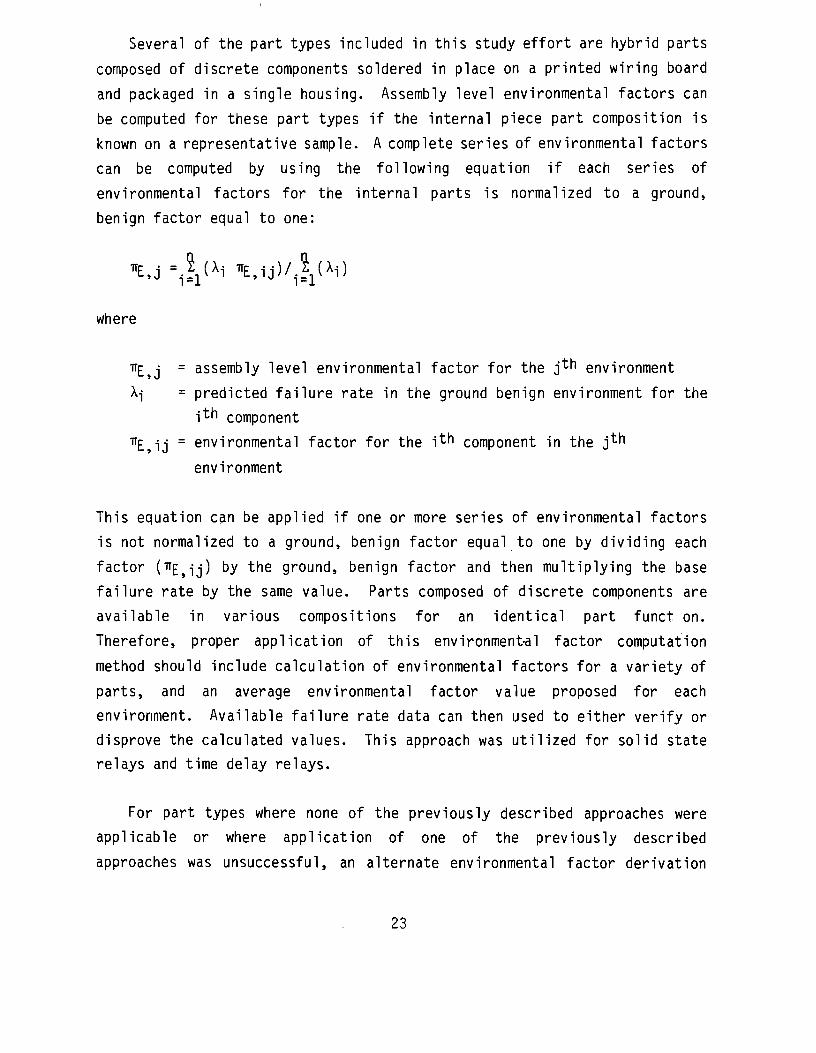
Several of the part types included in this study effort are hybrid parts
composed of discrete components soldered in place on a printed wiring board
and packaged in a single housing. Assembly level environmental factors can
be computed for these part types if the internal piece part composition is
known on a representative sample. A complete series of environmental factors
can be computed by using the following equation if each series of
environmental factors for the internal parts is normalized to a ground,
benign factor equal to one:
"EJ =.\(M ^ijO/.^x-i)
where
TTE^J = assembly level environmental factor for the jth environment
X-j = predicted failure rate in the ground benign environment for the
i^1 component
"E ij = environmental factor for the ith component in the jth
environment
This equation can be applied if one or more series of environmental factors
is not normalized to a ground, benign factor equal to one by dividing each
factor (^Ejij) by the ground, benign factor and then multiplying the base
failure rate by the same value. Parts composed of discrete components are
available in various compositions for an identical part funct on.
Therefore, proper application of this environmental factor computation
method should include calculation of environmental factors for a variety of
parts, and an average environmental factor value proposed for each
environment. Available failure rate data can then used to either verify or
disprove the calculated values. This approach was utilized for solid state
relays and time delay relays.
For part types where none of the previously described approaches were
applicable or where application of one of the previously described
approaches was unsuccessful, an alternate environmental factor derivation
23

process was developed. The alternate approach was based on the assumption
that an environmental factor relation can be determined where environmental
factor is a function of the "environmental stress ratios" obtained from
Reference 5 and presented in Table 3.3-1. The environmental stress ratio is
a relative index of combined environmental stress severity. The numerical
environmental stress ratio values were determined by Martin Marietta
Corporation, Orlando FL based on a survey of reliability experts. The survey
results provide a possible ranking of environmental factors to be applied in
cases where only limited data resources are available. The survey results
also provide a quantitative measure of the relative differences between
expected failure rate for different environments. To determine absolute (as
compared to relative) numerical environmental factor values, field failure
rate data are required from a minimum of four different environment
categories. The methodology to be described in the following paragraph can
be applied when data are available from two or three environments. However,
without data from a minimum of four environments, biased data in an
individual environment category can result in an environmental factor
relation which is essentially nonsense.
The numerical failure rate data from the different environment
categories should be similar in regard to all significant failure rate model
parameters except for environment. If there are apparent differences other
than environment, then the data should be normalized to compensate for the
apparent differences. Thus, the numerical differences between the data
points are primarily a function of the effect of environmental stress and
statistical noise. A regression analysis is then preformed where the
environmental stress ratio is the independent variable and the normalized
failure rate is the dependent variable. By applying different
transformations on the dependent and independent variable, the environmental
factor relation can be changed to several general forms. Three examples of
environmental factor relation form are given below:
1) Xn = K TTE = AS + B
2) Xn = K TTE = A(S)B
3) Xn = K TTE = A exp(BS)
24

where
Xn = predicted normalized failure rate
K = normalization constant
Tr£ = environmental factor
S = environmental stress ratio
A,B = regression contants
TABLE 3.3-1: ENVIRONMENTAL STRESS RATIOS
Environment
ground, benign ground, fixed ground, mobile manpack naval, sheltered naval, unsheltered naval, undersea, unsheltered naval, benign, submarine naval, hydrofoil airborne, inhabited, transport (1) airborne, inhabited, fighter (2) airborne, uninhabited, transport (1) airborne, uninhabited, fighter (2) airborne, rotary wing missile, launch cannon, launch undersea, launch missile, free flight airbreathing missile, flight space, flight
Notes: (1) includes bomber and cargo aircrafts (2) includes attack, trainer and fighter aircrafts
Abbreviation
GB GF GM MP NS NU NUU NSB NH AIT AIF AUT AUF ARW ML
• CL USL MFF MFA SF
Rank
1 3 7 8 5 10 14 4 12 6 13 15 17 16 19 20 18 9 11 2
Environmental Stress Ratio
1.0 2.7 11.5 12.5 7.3 16.8 20.6 6.0 19.2 10.2 19.5 23.1 33.5 27.6 42.7 720.6 37.1 12.6 17.6 2.1
The correlation coefficient is used as a measure of relative fit between the
regression solutions and the normalized failure rates.
The results of this environmental factor derivation process can be used
in two basic ways. In the instance where data are available from relatively
few environment categories, but the data are of high quality, the
environmental factor derivation process can be used to determine
25

environmental factors for only those environment categories without data.
In the instances where data are available from more environment categories,
but are of questionable quality, then the environmental factor derivation
process can be used to derive the entire set of environmental factors. In
those instances, it can be assumed that the observed environmental factors
which are too high or too low cancel each other out, and therefore, the
regression solution represents the best estimates for environmental factor.
The environmental factor derivation process was used to derive the
environmental factors for filters, meters, fuses, crystals and incandescent
lamps. This process has two major deficiencies. First, the numerical rank
of environment factors derived by this method are the same for all part
types. In practice, the rankings of environmental factors are similar for
most part types, but not identical. The second deficiency is that the
environmental stress ratios were determined before the release of Reference
4. Reference 4 recommended that the four original avionic environmental
factors be replaced by ten factors. Environmental stress ratios given in
Reference 5 are only available for four avionic environments (airborne
inhabited fighter, airborne inhabited transport, airborne uninhabited
fighter, airborne uninhabited transport). Therefore, each series of
environmental factors derived by this method proposes fixed inhabited and
uninhabited values for the original fighter (attack, trainer and fighter)
and transport (cargo and bomber) environment categories.
In conclusion, environmental factors were determined for each part type
considered in this study except neon lamps. Table 3.3-2 presents a summary
showing method of environmental factor development versus part type. Each
section of this report pertaining to model development includes a discussion
of the method used to determine the applicable environmental factors.
3.4 References
1. Draper, N.R. and H. Smith, Applied Regression Analysis, Wiley, 1966.
26
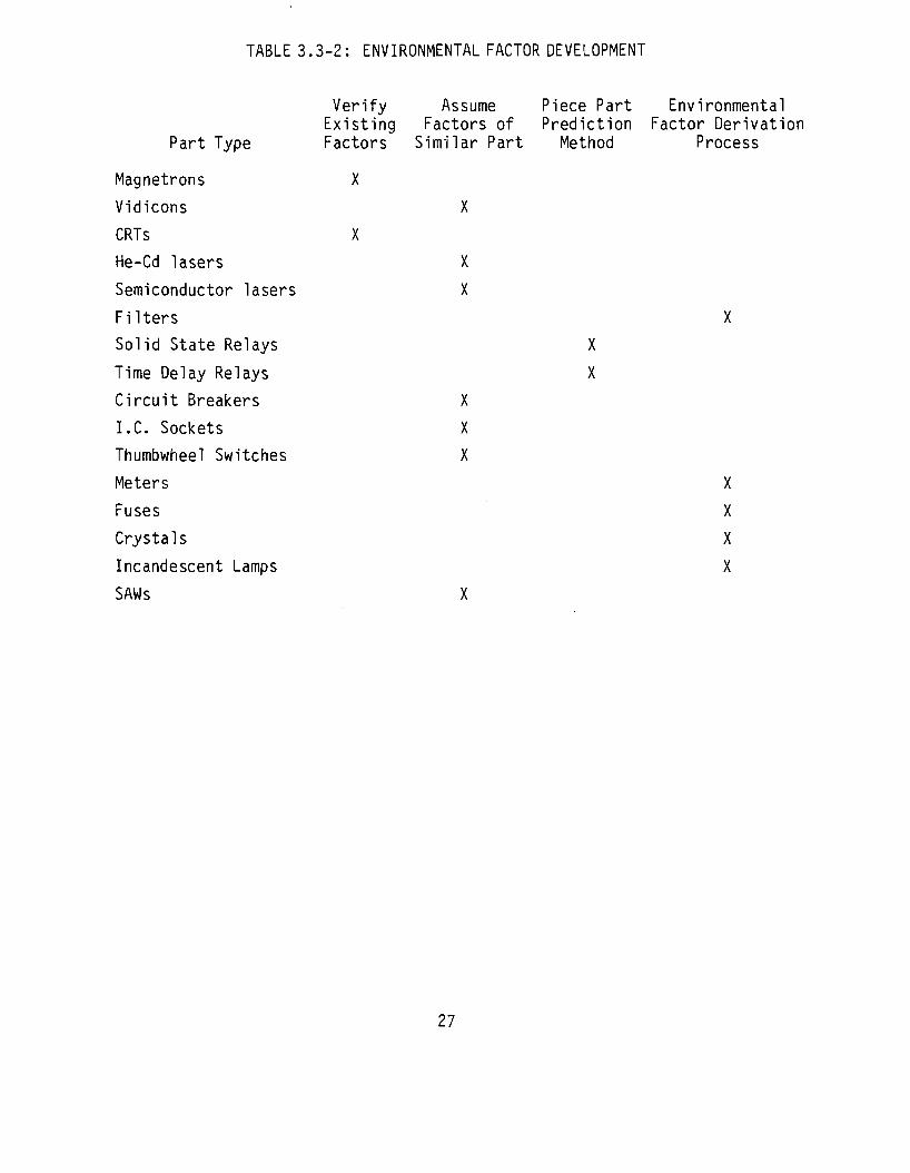
TABLE 3.3-2: ENVIRONMENTAL FACTOR DEVELOPMENT
Part Type
Magnetrons
Vidicons
CRTs
He-Cd lasers
Semiconductor lasers
Filters
Solid State Relays
Time Delay Relays
Circuit Breakers
I.C. Sockets
Thumbwheel Switches
Meters
Fuses
Crystals
Incandescent Lamps
SAWs
Verify Existing Factors
X
X
Assume Factors of
Similar Part
X
X
X
X
X X
X
Piece Part Prediction
Method
X
X
Environmental Factor Derivation
Process
X
X
X
X
X
27

Siegel, S., Non-Parametric Statistics for the Behavioral Sciences, McGraw-Hill, 1955.
Dey, K.A., Statistical Analysis of Noisy and Incomplete Failure Data, 1982 Proceedings, Annual Reliability and Maintainability Symposium.
Edwards, E., S. Flint and J. Steinkirchner, Avionic Environmental Factors for MIL-HDBK-217, Final Technical Report, RADC-TR-81-374, January, 1982.
Kremp, B.F. and E.W. Kimball, Revision of Environmental Factors for MIL-HDBK-217B, Final Technical Report, RADC-TR-80-299, September, 1980.
28

4.0 MAGNETRONS
4.1 Device Description
A magnetron is in effect a diode with the input electrodes being a
cathode and an anode. The high frequency is usually taken from a magnetron
by means of either a coaxial line or a waveguide. There have also been
magnetrons that employed special radiators to deflect the high frequency
energy. The magetron has the advantage over other microwave tubes in that it
is relatively simple to operate and has relatively low internal resistance.
Its primary disadvantage is the extent to which it can be electronically
tuned. Magnetrons are available which can be operated under either CW or
pulsed conditions. Some tubes are small enough to be held in the hand while
others are so heavy they must be picked up by mechanical means. The
operating voltage for the tubes range from a few hundred volts to many tens
of thousands of volts. Magnetrons may have the magnetic source attached to
the tube to form a complete unit or the magnet may be separate.
Pulsed magnetrons have been developed covering frequency ranges from a
few hundred MHz to 100 GHz. Peak power from a few KW to several megawatts
have been obtained with typical efficiencies of 30 - 40%. Continuous wave
magnetrons have also been developed with power levels of a few hundred watts
in tunable tubes at an efficiency of 30%. Pulsed magnetrons are used
primarily in radar applications as sources of peak power. Pulsed modulation
is obtained by applying a negative rectangular voltage pulse to the cathode
with the anode at ground potential.
Magnetrons may be either fixed frequency, mechanically tunable or
electrically tunable. Mechanical tuning of conventional magnetrons can be
accomplished by moving capacitive tuners near the anode straps or capacitive
regions of the quarter wave resonators. Tuner motion is produced by a
mechanical connection through flexible bellows in the vacuum wall. Voltage
tunable magnetrons use a circular-format, re-entrant stream injected beam
which interacts with a standing wave on a low Q resonant structure.
29
Pulsed magnetrons are available in both conventional and coaxial
designs. Coaxial magnetrons differ from conventional magnetrons in that
they have an internal stabilizing cavity. The stabilizing cavity greatly
improves frequency stability. The coaxial design also includes higher
efficiency, improved r-f output spectrum and longer life as its attributes.
4.2 Failure Modes and Mechanisms
A magnetron tends to react to total incident energy, and to some degree
is affected by variations in heat, radiation and each power supply as if they
were signals. Similarly, variations in external electric and magnetic
fields may affect performance. Therefore, application environment has a
significant effect on magnetron performance. Proper magnetron selection for
a particular application environment minimizes the effects of environmental
stress.
The reason for the envelope and seals is to provide electrical and
magnetic insulation and protect the electron ballistics by keeping the
vacuum within the tube constant. Loss of vacuum may occur due to
deterioration of a seal or a puncture or crack in the envelope. The
deterioration of a seal and the subsequent loss of vacuum is a function of
the seal type, length of the seal, thermal cycling, ambient temperature and
number of pins in the connector. The tube envelope, the seal, the filament
and in some cases, the cathode may be damaged by shock and/or vibration.
A partial loss of seal will result in a contaminated environment which
may poison the cathode or cause the filament to burn-up and which may result
in either tube degradation or catastrophic failure. The cathode must be
capable of carrying high current densities, especially in pulsed operation,
and be able to withstand considerable bombardment by electrons. An emissive
coating is required which will quickly recover in the event of poisoning and
which is also highly conductive, electrically and thermally; otherwise the
potential difference across the emissive coating may result in breakdown
through the coating. Good thermal conductivity is necessary to prevent the
30
surface of the cathode from becoming overheated which leads to either melting
or deterioration. The factors that influence cathode life are cathode
bombardment which may be accelerated by mismatches in output coupling and
cathode temperature.
The filament provides thermal energy sufficient to excite the electrons
in the cathode to a state where some of the electrons obtain enough energy to
escape. The primary failure mode of the filament is an open and its
occurence is a function of temperature cycling, oxidation, shock, vibration,
applied power and method of applying power.
The magnetic circuit may be an integral part of the tube or it may be a
separate device. In either case, the failure or degradation of the magnetic
circuit may result in catastrophic failure or degradation in tube operation.
For example, if the magnetic field strength is too low the magnetron will
oscillate in another mode than the IT mode, or the efficiency will be low. If
the field strength is too high, the appropriate anode voltage will also be
too high and there will be a risk of anode flashover.
4.3 Magnetron Failure Rate Prediction Model
This section presents the proposed failure rate prediction model for
magnetrons. The proposed model is:
Xp = Xb TTU TTE TTC
where
Xp = magnetron failure rate (failures/10^ filament hours)
TTU = utilization factor (see Table 4.3-1)
TTE = environmental factor (see Table 4.3-2)
31

TTC = construction factor
= 1, CW magnetrons (rated power < 5 kw)
= 1, coaxial pulsed magnetrons
= 5.4, conventional pulsed magnetrons
Xb = base failure rate (failures/10^ filament hours)
= 18, CW magnetrons (rated power < 5 kw)
= 19 ( f ) 0 , 7 3 ( P ) 0 ' 2 0 , pulsed magnetrons
where
f = frequency (GHz)
P = rated peak power (Mw)
TABLE 4.3-1: UTILIZATION FACTOR
Utilization IT
(radiate hrs./filament hrs.)
0.0
0.1
0.2
0.3
0.4
0.5
0.6
0.7
0.8
0.9
1.0
0.44
0.50
0.55
0.61
0.66
0.72
0.78
0.83
0.89
0.94
1.0
TTU = 0.44 + 0.56 (R), R = radiate hrs./filament hrs.
32

TABLE 4.3-2: ENVIRONMENTAL FACTOR
Environment
GB
GF
GM
Mp
NSB NS
Nu
NH
NUU
ARW
AlC
AIT
AlB
TTE
1.0
2.0
4.0
36
13
13
20
56
60
80
11
13
15
Environment
AlA
AlF
AUC
AUT
AUB
AUA
AUF
SF
MFF
MFA
USL ML
CL
4.4 Failure Rate Model Development
The approach utilized for model development of magnetrons was to
identify significant variables by analysis of "magnetron failure rate data.
The model parameters were quantified with the same data. At the conclusion
of each step, the results were given a thorough theoretical analysis. The
magnetron failure rate data collected in support of this study is presented
in Table 4.4-1. Life test data supplied by magnetron manufacturers and field
experience data received from Sacramento ALC and summarized by IITRI
comprised the majority of all collected data.
Application and construction variables were identified for magnetrons
and are presented in Table 4.4-2. These variables represent possible failure
rate model parameters whose values were determined whenever possible for all
collected data.
TTE
4.0
20
13
16
19
5.0
30
1.0
36
50
106
160
2000
33
TABLE 4.4-1: MAGNETRON FAILURE RATE OATA
ENTRY NO.
1 2 3 4 5 6 7 8 9
10 11 12 13 14 15 16 17 18 19 20 21 22 23 24 25 26 27 28 29 30 31 32 33 34 35 36 37 38 39 40 41 42 43 44 45 46 47 48 49 50 51 52 53 54 55 56 57 5B 59 60 61 62
(6) (6)
(6)
(6) (6) (6)
(6)
(6)
63 ( 6 )
64 65 66 67 68 69 70 71 72 73 74 75 76 77 78 79 80 81 B2 83 84 85 86 87 88 89
TTPE (1 )
C.W. Conv.
" " " " " " " " " " " " " C.W.
Conv.
" " " " " " •
" " " " " " " " " •
" " ° " " " " " " " " " " " Coax.
" " "
" " " " " " Conv. •
" " " " " " •
" " " " " •
" •
" "
FREQUENCY (GHz)
4.31 8.83 9.05 9.35 3.05 3.05 6.43 1.29 2.80 3.30 9.32 8.80 5.64 2.81 1.30 9.08 2.78
(7) 2.80 2.80 2.81 2.B1 2.81 2.81 2.81 2.81 2.81 2.81 2.81 2.B1 2.BO 2.80 2.78 2.78 2.78 2.78 2.78 2.78 2.78 2.78 2.7B 2.78 2.B1 2.B1 2.81 2.B1 2.81 2.81 2.B1 2.81 2.81 2.B1 2.BO 2.80 2.80 2.BO 2.80 2.80 2.80 2.80 2.BO 2.80 2.80 2.80 2.80 1.30 1.30 1.30 1.30 1.30 1.30 1.30 1.30 2.80 2.BO 2.80 2.80 2.BO 2.BO 2.80 2.80 3.30 2.80 2.80 2.80 2.80 2.80 2.BO 2.80
PEAK POWER LEVEL U w )
< 1 40 40 40 20 50
180 400 800
1000 250
1 175
4500 1000
40 3500
< 1 800 BOO
4500 4500 4500 4500 4500 4500 4500 4500 4500 4500
800 BOO
3500 3500 3500 3500 3500 3500 3500 3500 3500 3500 4500 4500 4500 4500 4500 4500 4500 4500 4500 4500 3000 3000 3000 3000 3000 3000 3000 3000 3000 3000 3000 3000 3000 1000 1000 1000 1000 1000 1000 1000 1000 800 800 800 800 800 800 800 800
1000 800 800 BOO 800 800 800 800
TUNING (2)
E lec . None Mech. None
" " " Hech.
" " None
Mech. Mech. None Mech.
" "
(7) Hech.
" None
" " " " " " " " " None
" Mech.
" * " " " " " " " None
" "
Mech.
COOLING (3 )
None F.A.
" " " " " " " " " " " Liquid
F.A.
" Liquid None F.A.
" Liquid
" " " " M
" " " '•
F.A.
" Liquid
" " " " " " " " " " " " " " " " " " " " " " " " " " " " " " 11
* F.A.
" " ••
" " " " " * " " " • * • " • h
* • •
"
R ( 4 )
1.0 1.0 1.0 1.0 1.0 1.0 1.0 1.0 1.0 1.0 1.0 1.0 1.0 1.0 1.0 1.0 1.0 1.0 0.B5 0.95 0.09 0.14 0.25 0.37 0.46 0.53 0.65 0.75 0.85 0.95 0.85 0.95 O.OB 0.19 0.27 0.37 0.47 0.54 0.65 0.75 0.85 0.95 0.07 0.17 0.29 0.32 0.45 0.55 0.67 0.7B 0.85 0.95 0.06 0.16 0.34 0.48 0.69 0.76 0.89 0.95 0.33 0.50 0.67 0.89 0.97 0.22 0.39 0.42 0.55 0.65 0.74 0.86 0.95 0.06 0.16 0.26 0.36 0.45 0.55 0.65 0.75 0.04 0.19 0.24 0.37 0.45 0.55 0.65 0.7B
ENVIRONMENT
G8 G8 GB GB GB GB GB GB GE GB GB GB GB GB GB GB GB GF GF GF GF GF GF GF GF GF GF GF GF GF GF GF GF GF GF GF GF GF GF GF GF GF GF GF GF GF GF GF GF GF GF
• GF GF GF GF GF GF GF GF GF GF GF GF GF GF GM GM GM GM GM GM GM GM GM GM GM GM GM GM GM GM GM
"GM GM GM GM GM GM GM
PART NO.
6177A 2J50
2J51A 2J55
2J70A 2J70B
4J58 5J26 5586 5795 6002 6248 6344
6410A 6517 7256 7529
(7) 55B6 5586
6410A 6410A 6410A 6410A 6410A 6410A 6410A 6410A 6410A 6410A
8798 8798
QK-327A QK-327A QK-327A QK-327A QK-327A QK-327A QK-327A QK-327A 0K-327A QK-327A QK-338A QK-338A QK-33BA QK-338A QK-338A 0K-338A 0K-338A 0K-338A QK-33BA QK-338A
VMS-1143A VMS-1143A VMS-1143A VMS-1143A VMS-1143A VMS-U43A VMS-1143A VMS-U43A VMS-1143B VMS-1143B VMS-1143B VMS-1143B VHS-U43B
400615 400615 400615 400615 400615 400615 400615 400615
5586 5586 5586 5586 5586 5586 55B6 5586 5795 8798 8798 8798 B798 B798 879 B 8796
FAILURES
2 0 0 1 0 3 0 0 0 2 0 4 2 3 0 4 2 5
19 131
2 3 3 4 6 4
20 25 72
273 10 91
2 1 A 8 6 6
14 15 90
446 1 6
10 3 3
13 6 9
37 95
1 2 1 1 3 1 5
21 1 1 1 1 8 2 7 3
11 25 15 3 6 2 5
10 33 75 50 28 25 4 2 1
10 26 17 16 8
PART HOURS
(5)
84.000 3,500 3.500 5 .200 4.000
17.900 1,000 1.500 1,000 9 ,400 1.000
29.600 23.000
6,200 1.500
46,200 3,600
157,000 70 ,000
250,800 6.000
13,470 20.900
8,120 16.330 8,650
76,000 66 ,000
210,000 810,000
30.JS40 180,000
15,000 2 ,630
14,450 16,900 13.6B0 15,430 22,000 31,000
280,000 1 .150,000
3 ,430 16,700 31.800
9 ,150 13,810 26,000 12.570 28 ,580 74.000
250.000 46 ,900
217,000 56.600 43 ,380 17,130 31 ,900 86,700 40,000 10,000
5,630 1.500
64 ,100 73 ,560
7.010 34,950 10.860 16.920 77,750 52,400
3,470 19.850 9 ,440
10,500 49.120
126.820 280,000 170,000
94,000 50,000 37,250 11,300 3,460
49 ,750 110,000 67 ,000 55,000 26.250
34

TABLE 4.4-1: MAGNETRON FAILURE RATE DATA (CONT'D)
ENTRY NO.
90 91 92 93 94 95 96 97 98 99
100 101 102 103 104 105 106 107 108 109
(6)
TOTALS
TYPE (1 )
Coax.
" " " " •
" •
" " " " •
" " " " •
FREQUENCY (GHz)
5.64 5.64 9 .05 9 .05 9 .05 9 .05 9 .05 9 .05 9 .05
(8) (8) (8) (8) (8)
i8! US (8) . ( 8 )
(8) (8)
PEAK POUER LEVEL ( K M )
1000 1000 200 200 200 200 200 200 200
1500 1500 1500 1500 1500 1500 1000 1000 1000 1000 1000
TUNING (2 )
Kech.
" E)ec.
" * " " " "
None
" " " " " " " " *
COOLING ( 3 )
F.A.
" " " * H H
" " " " •
" " " H
•* " "
R (4 )
0.04 0 .25 0 .15 0.24 0 .36 0 .50 0 .58 0 .65 0.74 0 .06 0 .18 0 .25 0 .36 0.49 0.54 D.19 0 .25 0 .36 0 .46 0 .55
ENVIRONMENT
GM GM GM GM GM GM GM GM GM GM GM GM GM GM GM GM GM GM GM GM
PART NO.
SFO-313 SFD-313 SFD-354 SFD-354 SFD-354 SFD-354 SFD-354 SFD-354 SFD-354 SFD-369 SFD-369 SFD-369 SFD-369 SFD-369 SFD-369 SFD-385 SFD-385 SFD-385 SFD-385 SFD-385
FAILURES
1950
PART HOURS (5)
43.300 8,000 3.400
23.000 2,200 1,170 6.120 3,410 4 ,560
12.730 70,240 66,850 51.620 42,610 25,250 63.680
157,300 28,810 33,020
9 ,220
6 ,940 ,930
NOTES:
( 1 ) C.W. - continuous wave, Conv. • convent iona l . Coax. * coax ia l ( 2 ) E l e c * e l e c t r i c a l , Hech. * mechanical (3) F.A. • forced air (4) R • radiate hours/filament hours, filament hours - radiate hours + standby hours
(5) filament hours, radiate hours * (R) x (filament hours) (6) insufficient part hours to introduce into the regression analysis (7 ) unknown (8) operating frequency is classified for SFD-369 and SFD-385 magnetrons
35

TABLE 4.4-2: MAGNETRON CONSTRUCTION AND APPLICATION VARIABLES
I. Operation Mode A. Continous Wave (CW) B. Pulsed
II. Type A. Conventional B. Coaxial
III. Tuning Availability A. No Tuning B. Mechanical Tuning C. Electrical Tuning
IV. Peak Power Level A. Rated B. Actual
V. Type of Output Port
VI. Magnetic Source Location A. Internal
B. External
VII. Tube Envelope Material
VIII. Tube Dimensions
IX. Heater Voltage Type and Level A. Rated Voltage B. Actual Voltage
X. Operating Temperature A. Rated
B. Actual
XI. Application Environment
XII. Ratio of Radiate hours to Filament hours
36
It was the intent of this study effort to analyze the effects of standby
operation on failure rate. The raw data for a particular tube type operating
in a similar application was merged according to the ratio of radiate
operating hours to filament operating hours. Standby operation for a
magnetron is the period of time when voltage is applied to the filament but
the magnetron is not radiating. Failure rates were calculated for each data
entry by dividing the observed failures by the filament hours. It was
assumed that a particular magnetron type operating under identical
conditions would exhibit a unique radiate and standby failure rate. It was
also assumed that the failure rate of magnetrons operating in the radiate
mode would be greater than the failure rate in the standby mode and that for
applications with intermediate amounts of standby operation the failure rate
would be a linear relation between the two extreme cases which are no standby
and total standby. Therefore a general magnetron failure rate prediction
model is given by,
Xp = (AR + B) Xb n TT2 •••
where
Xp = magnetron failure rate (failures/10^ filament hours)
R = radiate hours/filament hours
A,B = constants
Xb = base failure rate
iT-j = modifying factor(s)
An equation of this form is nonlinear and linear regression analysis can
not be directly applied. A brief discussion of nonlinear models is included
in Section 3.1. As suggested in Section 3.1, a linear equation form was used
to approximate the nonlinear part of the preliminary magnetron failure rate
prediction model. The approximation is as follows:
a(R)b = AR + B
37

where a, b, A and B are constants and R is the ratio of radiate to filament
hours. This approximation proved to be accurate for R values ranging from
0.2 to 1.0.
Stepwise multiple linear regression analysis was then applied to the
pulsed magnetron failure rate data. All data records, except where noted in
Table 4.4-1, were entered into the regression analysis. The variables which
were introduced into the regression are given in Table 4.4-3.
Three regression analyses were necessary. The initial regression
analysis identified frequency, rated peak power, magnetron type, ratio of
radiate to filament hours, environment and tuning as significant variables
at the 70% confidence level. The results from the initial regression were
rejected, however, as being inconsistent with theory. Strict interpertation
of the initial results were that fixed frequency and mechanically tunable
magnetrons have a similar failure rate and that electrically tunable
magnetrons have a failure rate 4.2 times as high. Also the results indicated
that magnetrons operating in a ground, benign and ground, fixed environments
have a similar failure rate and that magnetrons operating in a ground, mobile
environment have a failure rate 1.7 times as high. Both of these results
seemed to be inconsistent with theory. Mechanically and electrically
tunable magnetrons would both be expected to exhibit a higher observed
failure rate than fixed frequency magnetrons. However a factor of 4.2 is
unreasonable. Tunable magnetrons are similar to fixed frequency magnetrons
except with the addition of electrical or mechanical components. The
anticipated failure rates of the additional components are small in
comparison to the tube failure rate. Inspection of the raw data given in
Table 4.4-1 reveals that the only data entries with electrical tuning (data
entries 92-98) also operated in the ground, mobile environment. The
relatively higher failure rates computed for data entries 92 to 98 were
considered to be due to the application environment and not because of the
electrical tuning components. The reason for this apparent shortcoming in
the regression analysis is that a complete database for magnetrons was not
38

TABLE 4.4-3: MAGNETRON VARIABLE IDENTIFICATION
Parameter
frequency
rated peak power
type coaxial conventional
tuning fixed frequency mechanical electrical
environment GB GF GM
output port coaxial waveguide
cooling liquid forced air
radiate hrs/filament hrs
Variabl
X! = In
X2 = In
*3
X4. X5
X6, X7
x8
Xg
XlO = 1
e(s)
i(f)
i(P)
n(R)
Factor
(f) b l
(P)b2
exp(b3X3) 1.0 exp(b3)
exp(b4X4 + b5X5) 1.0 exp(b4) exp(b5)
exp(b6X6 + b7X7) 1.0 exp(b6) exp(b7)
exp(b8Xs) 1.0 exp(bs)
exp(bgXg) 1.0 exp(bg)
(R)bl°
39
obtained. To be able to evaluate both environment and tuning, data would
have to have been available for each tuning option in several different
environment categories.
A second regression analysis was preformed without tuning availability
as an input variable. The results from this analysis are given in Table 4.4-
4 and correspond to the following preliminary failure rate prediction model.
Each variable was significant at a 90% confidence level.
Xp = 15.5 (f)0' 7 3 2 (P)0-204 (exp(1>69X3)) ( R ) 0 - 3 6 0 ^
where
Xp = magnetron failure rate (failures/10^ hours)
f = frequency (GHz)
P = rated peak power (Mw)
X3 = 0, coaxial magnetrons
= 1, conventional magnetrons
R = radiate hours/filament hours
TT£ = environmental factor
= 1.0, GB
= 1.9, GF
= 3.2, GM
This preliminary model was then modified to resemble existing MIL-HDBK-217D
models.
TABLE 4.4-4: RESULTS OF THE REGRESSION ANALYSIS
Variable (Xi)
Xl X2 X3 X6 X7 xio
Constant
Coefficient (bi)
0.7318 0.2039 1.6887 0.6302 1.1543 0.3602 2.7406
Standard Error
0.2123 0.938 0.1701 0.3273 0.2876 0.0866
__
F-Ratio
11.88 4.73 98.50 3.71
16.11 17.66
__
40

The observed relationship between failure rate and ratio of radiate
hours to filament hours was designated as the utilization factor. It was
considered desirable to transform the approximate utilization factor form
(T7U = K(R)0,360) to the form originally assumed (T7U =•• AR + B). The
approximate model form was sufficiently accurate for the majority of ratio
values (R > 0.20). However, low ratio values resulted in approximate
utilization factor values approaching zero. Therefore, a utilization factor
of the assumed form was deemed necessary. A third regression analysis was
performed to obtain numerical estimates for the utilization factor
constants. All data entries were normalized for frequency, rated peak power,
magnetron type and environment. The normalization function is,
V = X0/(15.5(f)°-732(P)0-204 (exp(b3X3))TTE) = AR + B
where
\) = observed magnetron failure rate
and the results of the regression analysis were,
V = 0.678 (R) + 0.533
It was desired that the utilization factor be normalized to a value of one
for applications where radiate hours equals filament hours. Therefore, the
following modification was made to the preliminary magnetron failure rate
prediction model.
V = 0.678 (R) + 0.533
TTU = 0.825 V = 0.560 (R) + 0.440
Xp = (15.5/0.825) ( f ) 0 - 7 3 2 ( p ) 0 - 2 0 4 ( e x p(1 .69X 3 ) ) TTU TTE
= 18.8 ( f ) 0 ' 7 3 2 (p)0-204 ( e x p ( 1 > 6 g X 3 ) ) ^ ^
41

It was decided to include frequency and rated peak power into an equation
for base failure rate. The magnetron base failure rate then becomes,
Xb - 18.8 ( f ) 0 ' 7 3 2 ( P ) 0 - 2 0 4
where
^b = base failure rate (failures/106 hours)
A construction factor ( c) was defined to account for magnetron type.
The equation ( T C = exp(1.69 X3)) when solved for X3 = 1 and 0 gives the
following construction factors:
conventional magnetron, 5.42
coaxial magnetron, 1.0
Data were collected from three environment categories. The observed
environmental factors along with upper and lower confidence limits are given
in Table 4.4-5.
TABLE 4.4-5: OBSERVED MAGNETRON ENVIRONMENTAL FACTORS
Environment L 20%CL observed \ U 8 0 % C L
GB — 1.0
GF 1.42 1.88 2.48
GM 2.49 3.17 4.05
The observed ground, fixed environmental factor and the observed ground,
benign environmental factor are consistent with the existing MIL-HDBK-217D
electron tube environmental factors. However, the magnitude of the observed
environmental factor for the ground mobile environment is significantly
lower than the existing MIL-HDBK-217D value. A probable explanation is that
proper mangetron selection can minimize the effects of environmental stress.
42

For other tube types, such as cathode ray tubes, an identical part type can
be used in a wide variety of environments. For magnetrons, different part
types with similar specifications can be obtained depending on the intended
application environment. Therefore proper selection of available magnetrons
is essential for minimizing the effects of the environment.
The existing MIL-HDBK-217D electron tube environmental factors cannot be
applied to magnetrons without introducing error. However, it is essential
that a complete set of environmental factors be developed so that a proposed
failure rate prediction model can apply to a maximum number of potential
applications. In order to determine a complete set of environmental factors,
a review was initiated of previous revisions of MIL-HDBK-217. MIL-HDBK-
217B, Notice 2 dated 17 March 1978 expanded the number of magnetron base
failure rate options from two to nine. Additionally, this revision of MIL-
HDBK-217 included the environmental factors presented in Table 4.4-6. Table
4.4-6 also includes the observed magnetron environmental factors, upper and
lower confidence intervals and the MIL-HDBK-217B, Notice 2 factors
normalized to a ground, benign value equal to one. Analysis of Table 4.4-6
resulted in the conclusion that these factors can be accurately applied to
magnetrons. For application environment options which were not included in
MIL-HDBK-217B, Notice 2, the existing MIL-HDBK-217D electron tube factors
are proposed except for the naval, submarine environment. The naval,
sheltered factor was also applied to the naval, submarine environment so the
environmental factor rankings are consistent with MIL-HDBK-217D. Use of
these factors should result in slightly pessismistic failure rate
calculations.
43
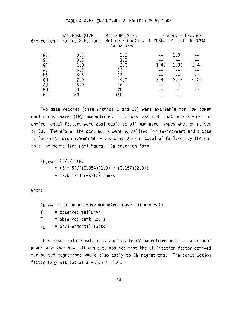
TABLE 4.4-6: ENVIRONMENTAL FACTOR COMPARISONS
MIL-HDBK-217B MIL-HDBK-217B Observed Factors Environment Notice 2 Factors Notice 2 Factors L 20%CL PT EST U 80%CL
Normalized
GB SF GF AI NS GM AU NU ML
0.5 0.5 1.0 6.5 6.5 2.0 8.0 10 80
1.0 1.0 2.0 13 12 4.0 16 20 160
— --
1.42 ----
2.49 --— --
1.0 --
1.88 ----
3.17 ------
----
2.48 ----
4.05 ----—
Two data records (data entries 1 and 18) were available for low power
continuous wave (CW) magnetrons. It was assumed that one series of
environmental factors were applicable to all magnetron types whether pulsed
or CW. Therefore, the part hours were normalized for environment and a base
failure rate was determined by dividing the sum total of failures by the sum
total of normalized part hours. In equation form,
xb,cw = 2f/(2T TTE)
= (2 + 5)/((0.084)(1.0) + (0.157)(2.0))
= 17.6 failures/10^ hours
where
xb,cw = continuous wave magnetron base failure rate
f = observed failures
T = observed part hours
•RE = environmental factor
This base failure rate only applies to CW magnetrons with a rated peak
power less than 5Kw. It was also assumed that the utilization factor derived
for pulsed magnetrons would also apply to CW magnetrons. The construction
factor (ire) was set at a value of 1.0.
44

Computation of the base failure rate for CW magnetrons completes the
magnetron failure rate prediction model development. The proposed model
represents magnetron failure rate as a function of magnetron type,
frequency, rated peak power, environment and amount of standby. The proposed
model increases prediction accuracy and extends prediction capabilities,
particularly in regard to coaxial and CW magnetrons, and it is recommended
that the proposed model be added to MIL-HDBK-217D.
4.5 References
1. Farney, George K., Crossed-Field Tubes, Electronics Engineers' Handbook, Second Edition, Fink, Donald 6. and Christiansen, Donald, McGraw-Hill, 1982.
45

5.0 VIDICONS
5.1 Device Description
The term vidicon is frequently used as a generic term for a
photoconductive camera tube. Vidicon is used to describe return beam
vidicons, lead oxide vidicons and silicon diode vidicons. In the usual
vidicon a homogeneous type of photoconductive layer is employed which will
freely accept the mobile photo generated carriers needed to replenish hose
extracted from the layers. The vidicon has many advantages compared to other
types of television tubes. It is relatively small in size, has a simple and
rugged structure, is low in cost and does not require critical adjustment in
operation. At the same time such tubes can produce high resolution images
and a high signal to noise ratio under proper illumination. In addition to
their use in black and white and color cameras for television pick ups,
vidicons are used with special photoconductors for pick up of images in the
infrared, ultraviolet and x-ray parts of the spectrum.
The basic elements of a typical vidicon tube are shown in the cross-
sectional diagram in Figure 5.1-1. The photoconductive layer is supported on
the glass face plate of the tube envelope. Between the photoconductor and
the faceplate a transparent electrode is provided, which acts as the target
back plate. In operation, the input image projected on to the photoconductor
produces conductivity variations in this layer causing previously
established surface charges to leak to the back plate. Upon recharging the
photoconductor surface to its equilibrium potential by the reading beam,
output voltage variations are produced across the load resistor connected to
the back plate. The scanning beam is usually focused and deflected by
magnetic coils. Tubes are also designed for operation with electrostatic
focusing and deflection, or electrostatic focusing and magnetic deflection.
The glass envelope of a typical vidicon is approximately one inch in diameter
and six inches in length, although there are vidicons with envelope diameters
ranging from approximately one-half to four and one-half inches.
46

Glass disk with storage layer ^ocus C01'
V///////A/S//A
Incident
light
L Ezzzzzzpzzza
Signal electrode Deflection coil
1
•Electron gun
^
Alignment coil
FIGURE 5.1-1: CROSS-SECTIONAL DIAGRAM OF A TYPICAL VIDICON
Prior to writing, the surface of the photoconductive layer is assumed to
be at zero potential, having been charged to this equilibrium potential
during previous scanning by the reading beam. With a dc voltage of +20V on
the back plate, a uniform electric field is established across the
photoconductor. During writing, an image of light or other radiation to
which the photoconductor is sensitive, is projected on to the
photoconductive layer. This generates free carriers. The resulting
increased conductivity allows a fraction of the local surface charge to leak
to the back plate, causing the surface to shift toward back plate potential.
A pattern of potential variations is thus established on the photoconductor
surface.
During reading, which is usually simultaneous with writing, the
photoconductor is scanned by the primary beam. Since the surface potential
of all photoconductors is low with respect to the reading gun cathode
potential, the secondary emission ratio is less than unity. Each of the
elements is thus shifted back to its equilibrium potential (i.e., the
potential of the reading gun cathode). As each element is shifted to ground
potential in scanning, a capacitive current is produced through the target
47
whose magnitude varies in accordance with the charge deposited by the beam.
These time varying currents in turn produce a half tone output signal voltage
across the load resistor. In normal operation, the scanning of the
photoconductor during reading acts to shift the elements down to a potential
which is close to the equilibrium (ground) potential. This automatically
erases stored information. Ideally this should be accomplished in a single
scan. In practice, several scans may be required to fully discharge or erase
the target because of the capacitance of the target and velocity spread of
the primary beam.
Relatively few target materials have been found which satisfy the
requirements imposed in the photoconductive layer by vidicons. To enable
charge storage, the dielectric relaxation time or R-C constant in the dark
must be considerably longer than frame time. For operation at conventional
TV frame rates, a target resistivity of approximately 10^2 n_Cm is required.
In addition, the response time of the photoconductor to changes in
illumination should be approximately a frame time or less to prevent lag or
image smear in the case of moving scenes. The choice of photoconductive
target material is the construction variable which best characterizes
vidicons. The following paragraphs present a brief description of the three
photoconductive materials most often used.
The photoconductor target material used in most commercial applications
is antimony trisulfide (Sb2$3). T n e material is relatively stable and has
spectral sensitivity peaked in the red between 700 - 800 nanometers (nm).
However, by evaporating the material in a residual gas atmosphere to form a
porous layer, its response can be shifted to 550 nm in the green. This will
more closely match the response of the eye. One of the limitations of Sb2$3
is its photoconductive decay time. After cutoff of the input light, several
TV frame times are required for the photoconductivity to fall to 10%.
Because of the long tail of the decay curve, objectionable image smear occurs
particularly at low input light levels.
48

The photoconductive material generally used in military applications is
a silicon diode array. Silicon target vidicons offer extremely high
sensitivity, low dark current, exceptional resistance to image burn and high
resolution capabilities. The spectral response for silicon target vidicons
ranges from 380 to 1100 nm. This broad spectral response range extends into
the near infrared.
For direct pick up of x-ray images a number of experimental vidicons have
been developed. One of the target materials is lead monoxide, (PbO). A
major problem associated with PbO targets is a fatigue effect whereby
irradiation of the layer with x-rays during application of voltage causes a
gradual increase in image persistence. This is also accompanied by a loss in
sensitivity and the development of nonuniformities. Such effects are
believed to be partially associated with the loss of oxygen from the PbO.
For pickup of color images, the input image is separated optically into three
color components. In operation, a single reading beam is used and the tube
is scanned in the same manner as a conventional vidicon. Output signals are
generated simultaneously across the three load resistors corresponding to
the three color components of the input image. One of the problems of such
tubes is signal lag caused by the relatively high layer capacitance of the
target junction. Vidicons with a PbO photoconductive material are often used
in applications when a clear, color picture is required.
5.2 Failure Modes and Mechanisms
Vidicons tend to react to total incident energy, and to some degree are
affected by variations in heat, light and radiation, and each power supply as
if the power supplies were signals. Similarly, variations in external
electrical and magnetic fields may affect performance. Therefore,
application environment has a significant effect on vidicon performance.
The function of the envelope and seals are to provide electrical
insulation and to protect the electron ballistics within the tube by keeping
the vacuum within the tube constant. Loss of vacuum may occur due to
49

deterioration of a seal or microcrack in the tube envelope. The
deterioration of a seal and the subsequent loss of vacuum is a function of
the seal type, vidicon bulb diameter, exposure to thermal cycling and ambient
temperature. A crack in the envelope may occur, especially in the neck area,
due to shock and/or vibration stresses. A partial loss of seal will result
in a contaminated internal tube environment which may poison the cathode or
the photoconductive target and may result in tube degradation or
catastrophic failure. Failure of the vidicon cathode accelerated by a
contaminated internal tube environment is the dominant failure mode for
vidicons.
Another important factor regarding vidicon reliability is that the
cathode must be capable of carrying high current densities and be able to
withstand considerable bombardment by electrons as well as by ions. An
emissive coating is required which will quickly recover in the event of
poisoning and is also highly conductive, electrically and thermally.
Otherwise, the potential difference across the emissive coating may result
in breakdown through the coating. Good thermal conductivity is necessary to
prevent the surface of the cathode from overheating, and then either melting
or deteriorating.
Exposure to shock or vibration may result in the repositioning of the
grids, electrodes and deflection plates. The repositioning of the grids,
electrodes and deflection plates may result in either performance
degradation or catastrophic failure depending on the magnitude of the
repositioning.
The filament provides thermal energy sufficient to excite the electrons
in the cathode to a state where some of the electrons obtain enough energy to
escape. The primary failure mode of the filament is an open. The frequency
of this failure mode is a function of temperature cycling, oxidation, shock,
vibration, applied power and method of applied power.
50

An important problem in vidicons is image lag caused by incomplete
discharge or shift of the photoconductive to equilibrium potential in a
single scan of the reading beam. This effect tends to be more noticeable at
low input levels when the magnitude of the potential pattern established in
writing is low. If the image lag phenomenon becomes severe, then the vidicon
must be replaced. Image lag is a degradation failure mechanism. To insure
adequate discharge of the photoconductive surface in a single scan, the total
capacitance of the target should be sufficiently low. Separate
consideration also requires that the photoconductive layer have a total
capacitance which never exceeds a certain value. This is based upon the fact
that sufficient charge must be deposited on the surface by the reading beam
to produce an output current substantially greater than the noise currents of
the load resister and video amplifier.
In the usual vidicon, the output signal increases linearly with
increasing input light. At high signal levels optical overloading occurs.
Optical overloading is defined as that illumination for which all of the
target plate shows effects that persist long enough for the human eye to
detect the persistence. As the intensity of a point in the field of view
increases, a level is reached where the output saturates. The output signal
no longer increases with input light. With further increase in source
intensity, the saturated point on the target material begins to spread into
surrounding areas because of lateral current flow in the photoconductive
target, internal reflections in the faceplate and flow in the output optics.
.This phenomenon is known as blooming and is most predominately noticed in
vidicons with Sb2S3 photoconductive material.
In operation, the target backplate potential is frequently varied to
produce optimum sensitivity and image quality. As the backplate voltage is
increased, the photocurrent is increased because of a higher electrical
field across the photoconductor. However, above a certain voltage the dark
current increases rapidly causing objectionable non-uniformities in the
picture background and reducing the signal to noise ratio. At low inputs the
51

operation of vidicons is limited by thermal noise generated by the load
resistor and the succeeding amplifier.
The most frequently observed failure modes for vidicons are degradation
modes. Therefore it would be anticipated that the instantaneous failure rate
function would be increasing in time. Unfortunately, data to support this
hypothesis is nonexistent. Therefore, the vidicon failure rate prediction
models to be presented in Section 5.3 represent an average failure rate with
respect to the anticipated equipment life. Time to failure data for cathode
ray tubes (which have certain construction similarities to vidicons)
indicate that the constant failure rate assumption does not introduce
significant errors.
5.3 Vidicon Failure Rate Prediction Model
This section presents the proposed failure rate prediction model for
vidicons. The proposed model only applies to vidicons with antimony
trisulfide (Sb2S3) or silicon diode array photoconductive materials. The
proposed model is:
xp = xb x ITE
where
•p = predicted vidicon failure rate in failures/106 hours
^b = base failure rate
= 51 failures/106 hours, Sb2S3 vidicons
= 48 failures/106 hours, silicon target vidicons
TE = environmental factor (see Table 5.3-1)
52
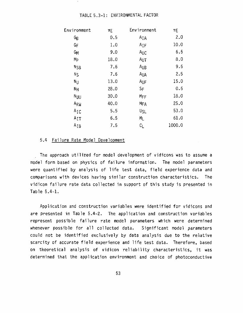
TABLE 5.3-1: ENVIRONMENTAL FACTOR
Environment
GB GF
GM
Mp
NSB Ns
Nu NH
NUU ARW
AlC AIT
AlB
TIE
0.5
1.0 9.0
18.0
7.6
7.6
13.0
28.0
30.0
40.0
5.5
6.5 7.5
Environment
AlA
AlF
AUC AUT
AUB AUA
AUF
SF
MFF
MFA
USL ML
CL
TTE
2.0
10.0
6.5
8.0
9.5
2.5
15.0
0.5
18.0
25.0
53.0
61.0
1000.0
5.4 Failure Rate Model Development
The approach utilized for model development of vidicons was to assume a
model form based on physics of failure information. The model parameters
were quantified by analysis of life test data, field experience data and
comparisons with devices having similar construction characteristics. The
vidicon failure rate data collected in support of this study is presented in
Table 5.4-1.
Application and construction variables were identified for vidicons and
are presented in Table 5.4-2. The application and construction variables
represent possible failure rate model parameters which were determined
whenever possible for all collected data. Significant model parameters
could not be identified exclusively by data analysis due to the relative
scarcity of accurate field experience and life test data. Therefore, based
on theoretical analysis of vidicon reliability characteristics, it was
determined that the application environment and choice of photoconductive
53

o o o
OH o 4 * f
o-
« C o - o -
I— u 1- - - -QJ o4 E —' E o o I ~
04 c\j
a. E QJ
QJ 4->
O
• — i — i — C O
V 4 - 4 - .£>
54

TABLE 5.4-2: VIDICON CONSTRUCTION AND APPLICATION VARIABLES
I. Photoconductive Material A. Chemical Compound
1. Sb2S3 2. PbO 3. Other
B. Silicon Semiconductor
II. Image Range A. Visible B. Infrared C. Ultraviolet D. X-Ray
III. Tube Dimensions A. Diameter B. Length
IV. Focus Method A. Magnetic B. Electrostatic
V. Deflection Method A. Magnetic B. Electrostatic
VI. Color vs. Black and White
VII. Heater Voltage and Current A. Rated B. Actual
VIII. Grid Voltages A. Rated B. Actual
IX. Temperature A. Rated
B. Actual
X. Application Environment
XI. Manufacturing Quality Level
55

material were the two dominate factors effecting vidicon failure rate. Many
other factors effect vidicon reliability, but the number of model parameters
is limited by the available data.
Failure rate data was collected from four different environment
categories. However, it was determined that there was insufficient
empirical data to develop a unique series of environmental factors for
vidicons. Therefore, the existing MIL-HDBK-217D environmental factors for
other tube types were analyzed to investigate whether they could be applied
to vidicons. A single series of environmental factors is currently applied
to all tube types included in MIL-HDBK-217D except for traveling wave tubes
(TWTs). It was assumed that these existing tube environmental factors could
also be applied to vidicons without introducing error because of
construction similarities with other tube types such as cathode ray tubes.
The additional avionic environmental factors presented in RADC-TR-81-374
(Ref. 1) were also included in the proposed vidicon failure rate prediction
model. Although the vidicon failure rate data presented in Table 5.4-1 is
not sufficient to confirm these factors, the data does appear to be in
agreement with the existing tube environmental factors.
The failure rate data (data entries 1, 2, 3, 4 and 5) were normalized for
environment and merged to determine base failure rate values for vidicons
with Sb2$3 and silicon diode photoconductive materials. No failure rate data
was available for vidicons with other photoconductive materials such as lead
oxide (PbO). Therefore, the proposed failure rate prediction model is
limited to vidicons with Sb2$3 and silicon diode photoconductive materials.
The normalized failure rate point estimates, lower 10% and upper 90%
confidence limit values are presented in Table 5.4-3.
TABLE 5.4-3: NORMALIZED FAILURE RATES
Base Failure Rates Photoconductive Normalized (F/106 hrs.)
Material Failures Part Hrs. (X106) L 10%CL PT EST U 90%CL
Sb2S3 456 9.423 45.51 48.39 51.42
Silicon Diode 18 0.350 36.48 51.43 70.58
56

The results presented in Table 5.4-3 are in complete agreement with the
anticipated failure modes and mechanisms of vidicons. As stated in Section
5.2, the dominant failure mode for vidicons is failure of the cathode, which
is physically similar for each vidicon type. Therefore, the results showing
that the normalized failure rates were numerically close was expected.
Degradation failure mechanisms associated with the photoconductive material
such as blooming and image lag are noticed more frequently with Sb2S3
photoconductive material. Therefore, the normalized failure rate for Sb2S3
vidicons being higher was also expected.
The homogeneity test for merging data described in Section 3.1 was
applied to the data (normalized for environment) to determine whether the two
base failure rate point estimates given in Table 5.4-3 differ significantly.
The results of the test indicate that the Kolmogorov-Smirnov statistic is
equal to 0.310 which is less than the critical value at 5% significance equal
to 0.565. This means that all normalized failure rate data could have been
merged. However, the point estimate base failure rates are in agreement with
theoretical analyses and show proper discrimination against device
construction. Therefore the optimal base failure rates to be applied to
vidicons are those given in Table 5.4-3 and the proposed vidicon failure rate
prediction model is,
Xp = Xb x TIE
where
Xp = predicted vidicon failure rate
Xb = base failure rate
= 48, Sb2S3 (antimony trisulfide) photoconductive material
= 51, silicon diode photoconductive material
TTE = environmental factors
= existing MIL-HDBK-217D electron tube factors.
57
All of the data collected were for mature vidicon devices. Since there
were no data available to prove or disprove the learning curve (TT|_) factor
currently in MIL-HDBK-217D, this factor was retained for the current model.
The proposed operating failure rate model then becomes:
X p = Xfo X TTE X TT[_
where
•p» ^b» " E and " L were defined in Section 5.3
The proposed failure rate prediction model for vidicons improves the
overall utility of MIL-HDBK-217D. The existing absence of a vidicon model
has impaired reliability prediction capabilities for surveillance equipments
like the AN/GXS-2 Ground Intrusion Detection system.
5.5 Bibl ioqraph.y
Dervishian, Ed, Some Simple, Practical Pointers for Routine Maintenance of Closed-Circuit TV, Plant Engineering, February, 1976, pp. 51-52.
McMann, Renville H., Jr., Television Cameras, Chapter 20, Electronics Engineers' Handbook, Second Edition, McGraw-Hill, 1982.
Welmer, Paul K., From Camera Tubes to Solid-State Sensors, RCA Review, Vol. 36, September, 1975.
Westinghouse Electric Corporation, Imaging Devices Product Catelog.
58
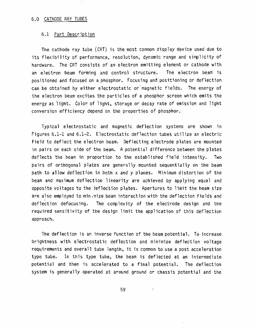
6.0 CATHODE RAY TUBES
6.1 Part Description
The cathode ray tube (CRT) is the most common display device used due to
its flexibility of performance, resolution, dynamic range and simplicity of
hardware. The CRT consists of an electron emitting element or cathode with
an electron beam forming and control structure. The electron beam is
positioned and focused on a phosphor. Focusing and positioning or deflection
can be obtained by either electrostatic or'magnetic fields. The energy of
the electron beam excites the particles of a phosphor screen which emits the
energy as light. Color of light, storage or decay rate of emission and light
conversion efficiency depend on the properties of phosphor.
Typical electrostatic and magnetic deflection systems are shown in
Figures 6.1-1 and 6.1-2. Electrostatic deflection tubes utilize an electric
field to deflect the electron beam. Deflecting electrode plates are mounted
in pairs on each side of the beam. A potential difference between the plates
deflects the beam in proportion to the established field intensity. Two
pairs of orthogonal plates are generally mounted sequentially on the beam
path to allow deflection in both x and y planes. Minimum distortion of the
beam and maximum deflection linearity are achieved by applying equal and
opposite voltages to the Jeflection plates. Apertures to limit the beam size
are also employed to minimize beam interaction with the deflection fields and
deflection defocusing. The complexity of the electrode design and the
required sensitivity of the design limit the application of this deflection
approach.
The deflection is an inverse function of the beam potential. To increase
brightness with electrostatic deflection and minimize deflection voltage
requirements and overall tube length, it is common to use a post acceleration
type tube. In this type tube, the beam is deflected at an intermediate
potential and then is accelerated to a final potential. The deflection
system is generally operated at around ground or chassis potential and the
59

electron gun is operated at a negative potential equivalent to the
intermediate accelerating voltage. To improve the linearity and beam focus,
a high resistance spiral is often used on the inside of the bulb between the
intermediate voltage anode and the final anode to obtain a linear post
acceleration field.
Electromagnetic deflection tubes have an electromagnet or deflection
yoke positioned around the neck of the tube to provide a magnetic field for
beam deflection. The deflection sensitivity of the magnetic tube is a linear
function of the magnetic flux density and length of the magnetic field and is
inversely proportional to the square root of the beam potential. Since the
deflection varies inversely as the square root of beam potential, the
advantage of post-acceleration with magnetic deflection is diminished as
compared with electrostatic deflection tube.
Dual electrostatic-magnetic deflection is sometimes used for special
purpose applications. Magnetic deflection is used for the major beam
positioning with electrostatic deflection utilized for low-angle or minor
deflection.
Focusing of the CRT electron beam is required to converge the beam into a
usable spot on the face since the initial beam from the electron gun is
diverging. Performance of the focusing system is a function of the ratio of
the distance between the focusing lens and the screen to the distance between
the focusing lens and the electron gun aperture.
The effective focus of the electron beam is limited by factors which are
not optical in nature. Maximum resolution of the beam is a function of the
current density and effective anode voltage. The space charge effect of the
electron beam limits the minimum size of the beam. The size of the object at
the CRT cathode also increases as the cathode current is increased.
Increasing the screen grid potential increases the resolution of the spot by
minimizing the effective aperture size of the electron beam at the expense of
increasing the modulation requirements for the control grid. Another factor
60

TRIODE EMISSION SYSTEM
HEATER-
CATHODE
LOW VOLTAGE ELECTRO STATIC FOCUS SYS?
ELECTROSTATIC DEFLECTION SYSTEM
PHOSPHOR SCREEEN ^*
CONTROL ELECTRODE
FOCUS ELECTRODE
DEFLECTION PLATES CONDUCTIVE BULB
WALL COATING
FIGURE 6.1-1: ELECTROSTATIC DEFLECTION SYSTEM
TRIODE EMISSION SYSTEM
MAGNETIC FOCUS SYSTEM
MAGNETIC DEFLECTION SYSTEM
ALUMINIZED PHOSPHOR SCREEN
HEATER V
CATHODE
/ CONTROL ELECTRODE
I FOCUS COIL
DEFLECTION COIL
ALIGNMENT COIL
CONDUCTIVE BULB WALL COATING
ANODE HIGH VOLTAGE CONNECTION
FIGURE 6.1-2: MAGNETIC DEFLECTION SYSTEM
61

limiting the focused resolution is the variation of the electron velocity and
the fact that the paths of all electrons in the beam are not symmetrical
around the center. Increasing the final anode voltage reduces the effect of
variations in the initial velocities and directions of the electrons in the
beam. CRT focusing is not analogous to optical focusing in that fields are
not sharply confined.
CRT focusing may be either electrostatic or magnetic. Electrostatic
focusing type tubes have either bipotential or unipotential guns. The
bipotential type has a tetrode type gun and offers high resolution and
moderate deflection defocusing. The unipotential CRT has a triode type gun
and offers medium resolution and low deflection defocusing. Magnetic
focusing tubes utilize an axial magnetic field concentric with the beam axis
of the CRT to converge the electron beam. In magnetic focusing, electrons at
an angle to the magnetic lines of force are deflected toward the line of the
magnetic field. Thus if the center line of the magnetic field is not
parallel and concentric with the center line of the beam, the beam shape and
resultant spot will be distorted and aberrations of the beam will occur.
Magnetic focusing generally provides better resolution, largely because the
magnetic focus coil is necessarily located further from the gun and the
magnification factor based on the ratio of object distance to image distance
has the lower number. However, the magnetic focus tube has the largest spot
growth or defocusing at the edge of the tube, owing to the larger beam bundle
in the magnetic focus lens and to the sharper crossover at the screen caused
by the lower ratio between the image distance and the object distance.
The major parameters for evaluation of deflection yokes are deflection
sensitivity, inductance and speed. Other parameters are the accuracy of the
orthogonality of the coils for xy deflection yokes, magnetic sensitivity,
coupling between othorgonal coils and deflection defocusing of the yoke.
Deflection defocusing of the CRT is a function of the uniformity of the
magnetic field and fringing fields. Fringe fields at the ends of the yoke
can be modified by shielding. However, such shields add time constants to
the magnetic field and produce non-linearities in fast sweeps or require
62

increased settling time for random positioning. Cathode ray tubes are
sensitive devices requiring careful shielding. Magnetic fields from
transformers, fans or servomotors may require shielding at both the source
and the tube. Fields from high current AC conductors near the tube may also
modulate the display. Generally the shield must cover both the area between
the yoke and gun and the bell of the tube near the face plate.
In the cathode ray tube the electron beam energy is converted to light by
a phosphor. The phosphor is a luminescent material in which the energy of
the electron beam is transferred to an electron in the phosphor crystal
raising the energy level of the electron. The electron then releases a
quantum of light energy when it returns to the initial or original state
subsequent to the excitation. The period of light emission from the phosphor
after excitation is termed the persistence of the phosphor. The nature of
persistence, or decay characteristic as a function of time, may vary from
logarithmic to exponential. The decay characteristic of phosphor is
affected by variables such as anode voltage, repetition rate, duration of the
excitation and current density of the electron beam. Selection of a phosphor
requires the balancing of several factors. Among these are color,
persistance, relative efficiency, resolution capability and its life time.
Phosphor life time or its durability is normally related to the sensitivity
of phosphor to overheating or burning. Since the efficiency of beam energy
conversion to light is fairly low, most electron beam energy is dissipated as
heat.
The contrast of a CRT is limited by reflected light from ambient
illumination and scattering of light emitted by phosphor in the face plate.
Light emitted from the written image results in halation or a series of
concentric rings around the beam spot. With large area beam writing, the
halation causes a general illumination of the phosphor reducing the CRT
contrast. Halation is the effect of specular reflection of light that
exceeds the critical angle of a glass-air interface. Another effect limiting
display visibility is light reflection from various glass-air interfaces.
63

Anti-reflection coatings such as magnesium fluoride reduce these
reflections.
The glass envelopes for CRT tubes are designed with a desired flat face
for the viewer and minimum glass thickness to reduce the weight of the
envelope. A flat face plate also leads to increased non-linearity and
pattern distortion. Glass envelopes are designed and tested to withstand
three to five times atmospheric pressure at a reasonable margin of safety. A
metal cone may be utilized for the bell of the CRT. A rim on the metal cone
supports the face plate, which is sealed to the rim under compression. This
seal increases the face plate resistance to implosion. The metal cone is
also self shielding to magnetic and electrostatic fields. The end of the
metal cone is protected and insulated for safety.
6.2 Failure Modes and Mechanisms
Cathode ray tube reliability depends on the performance of the electron-
optics and phosphor screen life time. Mechanical stresses may cause
implosion of the tube, or broken connections and filaments. Degradation of
the seals may cause cathode poisoning and eventually tube failure. Phosphor
brightness and durability reduce with time resulting in low brightness or
image distortion. High current densities cause burn-out and aging of the
phosphor resulting in the fall-off of brightness. External fields may cause
focusing degradation. Erosion and change in the characteristics of the
cathode may deteriorate the electron beam resulting in low brightness or
image distortion. An open filament (heater) causes a catastrophic failure.
The failure mechanisms most likely to be directly or indirectly
responsible for these failure modes are excessive heat and ambient
conditions. Both heat from the environment around the tube and heat
generated within the tube create this adverse effect. Internal heat rise is
due to one of two sources: the current flow from one element of the tube to
another element, and power used to raise the electron-emitting cathode to
operating temperature. The ambient conditions other than temperature that
64

are most likely to be directly or indirectly responsible for tube failure are
shock, vibration and electromagnetic fields.
6.3 Cathode Ray Tube Prediction Model
This section presents the proposed failure rate prediction model for
cathode ray tubes (CRTs). The proposed model is:
where
Xp = predicted CRT failure rate (F/106 hours)
Xt, = base failure rate (F/10^ hours)
= 9.6 F/106 hours
iTE = environmental factor (Table 6.3-1)
TT|_ = learning factor (Table 6.3-2)
6.4 Failure Rate Model Development
The approach utilized for model development was to identify significant
parameters by analysis of the CRT field experience failure rate data. The
model parameters were then quantified using the same data. At the conclusion
of each step, the results were given a thorough analysis to determine whether
they were consistent with the theoretical physics of failure information.
The CRT failure rate data collected in support of this study are presented in
Table 6.4-1.
Application and construction variables were identified for CRTs. These
variables which are listed in Table 6.4-2 represent factors which were
determined whenever possible for all collected data.
65

TABLE 6.3-1: ENVIRONMENTAL MODE FACTORS
Environment
GB
GF
GM
Mp NSB NS Nu NH NUU ARW
AlC AIT
AlB
TTE
0.5 1.0
9
18
7.6
7.6
13
28
30 40
5.5
6.5
7.5
Environment
AlA
AlF AUC AUT
AlIB
AUA
AUF SF
MFF
MFA
USL ML
CL
TTE
2
10
6.5
8
9.5
2.5
15
0.5
18 25
53
61
1000
TABLE 6.3-2: LEARNING FACTOR
t*(yrs) 1 2 3
TTL** 10 2.3 1
* t = number of years since introduction to military use
**TT|_ = lOt-2-1 for 1 <_ t £ 3
= 10 for t > 1
= 1 for t < 3
66
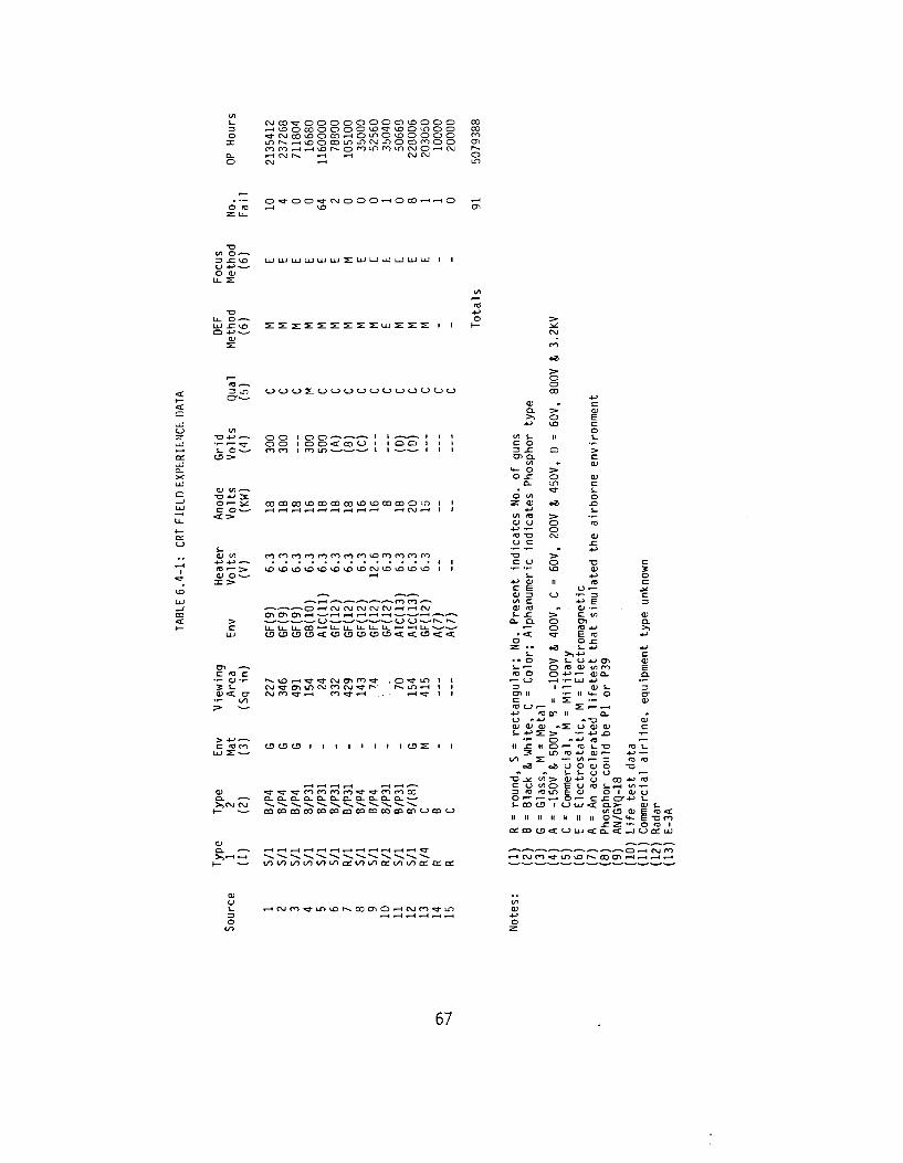
C \ J C 0 * 3 - O O O O O O O C 0 < X > O O O . — i ^ D O C O O O O O i - O ^ ^ D O L n O O * J C\J CO VD O CO i - l O L D O O O O O O
i n N H i o o c o m i n w i n o c o n o o
.—i CNJ r-. 1-H «-H C\J C\J
CM «—I
13 .C ^O LiJ L I 21 LU LlJ LU LlJ LU LlJ I I
LU . C KD O 4->
z z z s s s s s s i L u z z s : i i
3 L D <_><_><_>2 :<_><-><_><-><->oooooo c r —
•D •*-» — - O O I O O ^ - * ^ » ^ - I I .*~+*-*> I I l •r- r— q - O O • O O «C CO <-> < I O O I I >
i_ o — mm i n i n *—-—••—* i i • i • c o O l CL
0> V) -—. "O -»-> 3 o •— : * : COCOCO»£>COCOCO»£>*OCOCOOUD i P C O"^ - * r-t r-l ,—it—1 ,—( ,—f ,_( ,—( ,—( H ( \ J H I I
QJV) mmmmmmmm^ommmm 4-> 4-> *—* . | |
a; o — «-< z: >
-—*.—*-—*0 •—< C\J C\J C\J C\J CV «—< i—(CV o ^ e n o ^ f—i • * — * I - H •—i f—i f—i«—H •—»•*—»«—H ^—*«—«» ^ — * ^ _ * ^ _ ^ ^ _ * < _ ) - — . ^ _ ^ ^ _ * ^ _ * — . < _ ) <_) — r v . r-. U _ U _ U _ CO •—< U_ U_ U_ U_ LL. •—« >-H U_ •
C <0 C •t-OJ-f- r-.»£).—i«3-«3-c\JCT>cr>«3-JO*;3-il"> ' • 5 i _ c\j«3-cTiLOc\jmc\j«3-r-' J r-» m «—i i i 0>< cr c\j r o ^ t r - i en «3- «—i . H .—i «a- i i
a> ^ • ' f ^ T o r o n f O ' f c n f n c o CL — - Q.Q.Q.Q.Q_Q_0-Q-D-Q.Q. *—' >,C\J C\J " ^ *- " ^ " ^ *- *- " ^ ^ *- \ *- *-
(V fC J- -C
CL. CL
• <c o
z : • * i -
• • o J - •—
*o o •— <_> ZJ crt ii c fl <_?
4-»
(_) * QJ QJ J - 4->
— (0 4->
a> i _
• • >
o C > «3"
etfl
• >
<T >
O
1
It
cn
>
(L> • < -
C V) o> ra 4-> E (0 o j = i - 4->
>,4-> L. U W C f t « (D y i n 4-> r— Q) Q_ • r l i J + J »— 0> J-'<- 11 M- O Z ••-
z •— —* II CL.
• -o 2: o cu QJ
• - 4-> .O O * ^ -
i O •— fO J- -D LO *0 4-> QJ #—
: •-- w — =5 03 u o a; o
"O J>£ V) C U V ) 3 *0 IT3 o *— •—
I_ CO C3
It II II
a: co o
i - i - o o •— I S-.—I V) • o
LO fc a» o i a> .-t o •— c ^ cr-w
( <_> UJ < t CL>-
It 11 II 11 O ^ *f-
• «3 cC
: "D m <£<-3LU<CCL.eC_J<_3C£LiJ
t / ) to t / )LOt / )L^ ic t : t / ) t / )c t :LOLOci iccct :
H C \ j r o « 3 - i n t D M D c r i O i H f \ j r o ^ - i r >
67
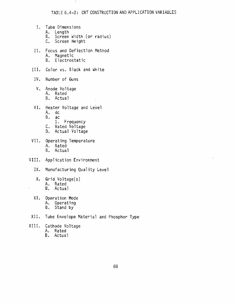
TABLE 6.4-2: CRT CONSTRUCTION AND APPLICATION VARIABLES
I. Tube Dimensions A. Length B. Screen Width (or radius) C. Screen Height
II. Focus and Deflection Method A. Magnetic
B. Electrostatic
III. Color vs. Black and White
IV. Number of Guns
V. Anode Voltage A. Rated B. Actual
VI. Heater Voltage and Level A. dc B. ac
1. Frequency C. Rated Voltage D. Actual Voltage
VII. Operating Temperature A. Rated
B. Actual
VIII. Application Environment
IX. Manufacturing Quality Level
X. Grid Voltage(s) A. Rated B. Actual
XI. Operation Mode A. Operating B. Stand by
XII. Tube Envelope Material and Phosphor Type
XIII. Cathode Voltage A. Rated B. Actual
68
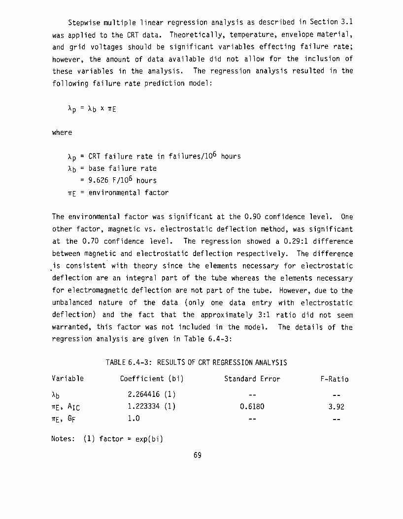
Stepwise multiple linear regression analysis as described in Section 3.1
was applied to the CRT data. Theoretically, temperature, envelope material,
and grid voltages should be significant variables effecting failure rate;
however, the amount of data available did not allow for the inclusion of
these variables in the analysis. The regression analysis resulted in the
following failure rate prediction model:
Xp = Xb X TTE
where
Xp = CRT failure rate in failures/106 hours
Xb = base failure rate
= 9.626 F/106 hours
iTE = environmental factor
The environmental factor was significant at the 0.90 confidence level. One
other factor, magnetic vs. electrostatic deflection method, was significant
at the 0.70 confidence level. The regression showed a 0.29:1 difference
between magnetic and electrostatic deflection respectively. The difference
is consistent with theory since the elements necessary for electrostatic
deflection are an integral part of the tube whereas the elements necessary
for electromagnetic deflection are not part of the tube. However, due to the
unbalanced nature of the data (only one data entry with electrostatic
deflection) and the fact that the approximately 3:1 ratio did not seem
warranted, this factor was not included in the model. The details of the
regression analysis are given in Table 6.4-3:
TABLE 6.4-3: RESULTS OF CRT REGRESSION ANALYSIS
Variable Coefficient (bi) Standard Error F-Ratio
Xb 2.264416 (1)
TTE, Aic 1.223334 (1) 0.6180 3.92
TTE, GF 1*0
Notes: (1) factor = exp(bi)
69
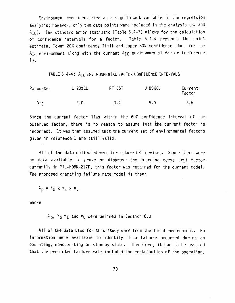
Environment was identified as a significant variable in the regression
analysis; however, only two data points were included in the analysis (GF and
A J Q ) . The standard error statistic (Table 6.4-3) allows for the calculation
of confidence intervals for a factor. Table 6.4-4 presents the point
estimate, lower 20% confidence limit and upper 80% confidence limit for the
Axe environment along with the current Aic environmental factor (reference
1).
TABLE 6.4-4: A I C ENVIRONMENTAL FACTOR CONFIDENCE INTERVALS
Parameter L 20%CL PT EST U 80%CL Current Factor
A I C 2.0 3.4 5.9 5.5
Since the current factor lies within the 60% confidence interval of the
observed factor, there is no reason to assume that the current factor is
incorrect. It was then assumed that the current set of environmental factors
given in reference 1 are still valid.
All of the data collected were for mature CRT devices. Since there were
no data available to prove or disprove the learning curve (TT[_) factor
currently in MIL-HDBK-217D, this factor was retained for the current model.
The proposed operating failure rate model is then:
Xp = Xb x *E * ^L
where
^p> ^b ^E anc' ^L w e r e defined in Section 6.3
All of the data used for this study were from the field environment. No
information were available to identify if a failure occurred during an
operating, nonoperating or standby state. Therefore, it had to be assumed
that the predicted failure rate included the contribution of the operating,
70
nonoperating and standby failures. The inclusion of any nonoperating or
standby failures should not bias the operating failure rate model too heavily
because 8 of the 11 data points used in the analysis were from systems that
normally operate 24 hrs/day 7 days/week, and one of the AJC data points (by
far the largest) was from the commercial airlines where equipment usage is
quite high (50%).
6.5 References and Bibliography
References
1. Edwards, E., et.al., Avionic Environmental Factors For MIL-HDBK-217, Final Technical Report, RADC-TR-81-374, January, 1982.
Bibliography
Annon., Determination of the Reliability Parameters for the 813H-1 CRT Assembly (CPN 618-1631-001).
Arno, Robert G., Nonelectronic Parts Reliability Data, Reliability Analysis Center Publication NPRD-2, Summer, 1981. Brain, Jake, Determining the Phospor Life of A Cathode Ray Tube, Thomas Electronics, Inc. Internal Report.
Corson, Bayard R., Some Reliability Characteristics of CRT Cathode Assemblies, IEEE Transactions on Reliability, Vol. R-23, No. 4, October, 1974, pp. 226-230.
Edwards, E., et.al., Avionic Environmental Factors For MIL-HDBK-217, Final Technical Report, RADC-TR-81-374, January, 1982.
Fink, Donald G., and Christianson, Donald, Editors, Electronics Engineers' Handbook, Second Edition, McGraw-Hill, 1982, Chapters 6, 7, 8, 9, 11, 20, 25.
Galves, J.P. and Brun, J., Reliabil ity of High-Brightness CRT's For Airborne Displays, AGARD-CP-261 Conference Proceedings, No. 261, April 1979, pp. 26-1 to 26-14.
I IT Research Institute, Electronic Reliability Design Handbook, Volume II, Contract Data Item, Contract F30602-78-C-0081, 1981.
Sinharoy, S., et. al., Surface Stability Studies on Some CRT Phosphors, Journal of Electrochemical Society: Sol id-State Science and Technology, January, 1981, pp. 205-208.
71
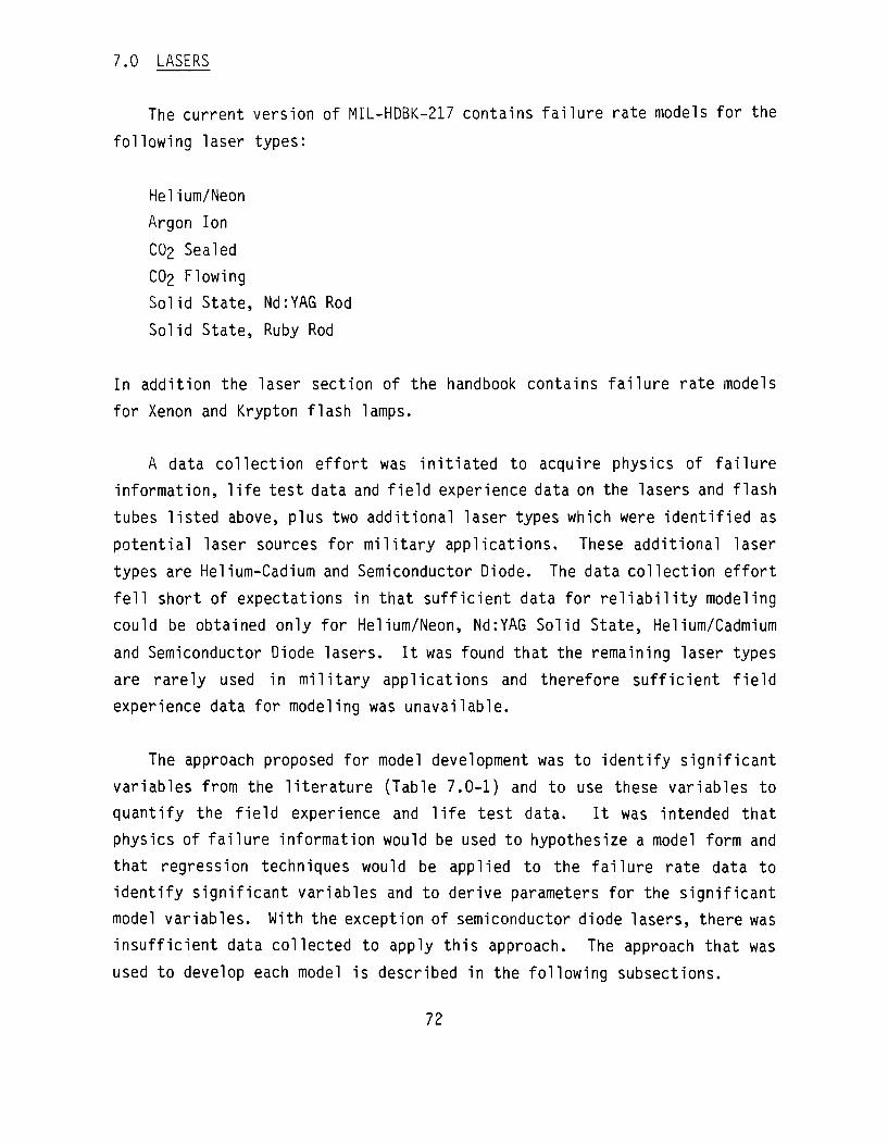
7.0 LASERS
The current version of MIL-HDBK-217 contains failure rate models for the
following laser types:
Helium/Neon
Argon Ion
CO2 Sealed
CO2 Flowing
Solid State, Nd:YAG Rod
Solid State, Ruby Rod
In addition the laser section of the handbook contains failure rate models
for Xenon and Krypton flash lamps.
A data collection effort was initiated to acquire physics of failure
information, life test data and field experience data on the lasers and flash
tubes listed above, plus two additional laser types which were identified as
potential laser sources for military applications. These additional laser
types are Helium-Cadium and Semiconductor Diode. The data collection effort
fell short of expectations in that sufficient data for reliability modeling
could be obtained only for Helium/Neon, Nd:YAG Solid State, Helium/Cadmium
and Semiconductor Diode lasers. It was found that the remaining laser types
are rarely used in military applications and therefore sufficient field
experience data for modeling was unavailable.
The approach proposed for model development was to identify significant
variables from the literature (Table 7.0-1) and to use these variables to
quantify the field experience and life test data. It was intended that
physics of failure information would be used to hypothesize a model form and
that regression techniques would be applied to the failure rate data to
identify significant variables and to derive parameters for the significant
model variables. With the exception of semiconductor diode lasers, there was
insufficient data collected to apply this approach. The approach that was
used to develop each model is described in the following subsections.
72

TABLE 7.0-1: LASER CONSTRUCTION AND APPLICATION VARIABLES
Type and Lasing Material
A. Solid 1. Lasing Material
B. Liquid 1. Lasing Material
C. Gas 1. Lasing Material
D. Semiconductor 1. Lasing Material
Power Level A. Continuous
1. Rated 2. Actual
B. Pulse 1. Rated 2. Actual
Rated Life A. Hours B. Pulses
Pumping Mechanism A. Type
1. Optical 2. Chemical 3. Electrical
a. Discharge i. Transverse
b. Current B. Components
1. List Quantity and Type 2. List Temperature and Stress Level for Each Component^
C. Number of Firings (flashes) 1. Rated 2. Actual
D. Output Energy Level 1. Rated 2. Actual
Material A. Tube
1. Quartz 2. Glass 3. Etc.
73

TABLE 7.0-1: LASER CONSTRUCTION AND APPLICATION VARIABLES (CONT'D)
B. Seal 1. Epoxy 2. Glass
C. Lens 1. Quantity
a. Quartz b. Glass
VI. Q-Switch A. Type
1. Electrooptical 2. Rotating Prism (mirror) 3. Acoustooptical 4. Saturable Absorber
B. Components 1. List Quantity and Type 2. List Temperature and Stress Levels for Each Component
VII. Firing Circuit (Pulse forming) A. Components
1. List Quantity and Type 2. List Temperature and Stress Levels for Each Component
VIII. Power Supply A. Components
1. List Quantity and Type 2. List Temperature and Stress Levels for Each Component
IX. Mirrors A. Quantity
1. Totally Reflective 2. Partially Reflective
B. Seal Type 1. Hermetic 2. Dust 3. None
C. Alignment 1. Adjustable 2. Nonadjustable
D. Material 1. List All Materials
a. Reflective b. Substrate
X. Cooling Circuit A. Type
1. Forced Air
74

TABLE 7.0-1: LASER CONSTRUCTION AND APPLICATION VARIABLES (CONT'D)
2. Liquid 3. Gas 4. None
B. Components 1. List Quantity and Type 2. List Temperature and Stress Levels for Each Component
XI. Auxiliary Circuits A. Type
1. Input/output Valves a. Liquid b. Gas
2. Mixing Chamber 3. Frequency Doubling Crystal
B. Components 1. List Quantity and Type 2. List Temperature and Stress Levels for Each Component
XII. Temperature (Ambient or Tube) A. Rated
B. Actual
XIII. Operating Environment
XIV. Manufacturing Quality Level
Additional Information
I. Part Designation A. Military B. Commercial
NOTE: 1) Temperature and Stress Level are those required to calculate a MIL-HDBK-217 Part Stress Level Failure Rate.
75

It is proposed that the current Argon Ion, CO2 Sealed, CO2 Flowing and
Solid State, Ruby Rod models be retained until sufficient field experience
data are available to reanalyze them.
7.1 Semiconductor Lasers
7.1.1 Device Description
Various semiconductor materials have been shown to exhibit laser
properties when an electric field is applied. These are sometimes referred
to as injection lasers. Semiconductor lasers are finding applications in
areas such as range-finding, pollution detection and communication. The
wide range of wavelengths obtainable, inherent simplicity of large scale
manufacture, compatibility with electronic circuitry and small size can be
expected to result in large scale applications.
The most common form of semiconductor laser consists of a p-type and n-
type material forming a p-n junction. Electrodes are attached to the
opposite faces of the material and are connected to a power supply (pulsed
and/or DC). When the p-n junction is forward biased optical radiation is
generated, electrons in the conduction band recombine with a hole in the
valence band to give a quantum of radiation with energy equal to the energy
difference between the two states. This radiation is called recombination
radiation. If a sufficient population inversion in the junction area is
achieved, (i.e. greater number of electrons in conduction band than holes in
the valence band), then recombination may be stimulated and laser action is
possible. The wavelength of the laser transition is determined by the size
of the band gap. One of the simplifications of diode lasers as compared to
other lasers is that no external mirrors are needed to provide feedback. The
high reflectivity due to the refractive index difference at the air-diode
interface is sufficient. The diodes are cleaved along material crystal
planes and the parallelism of the reflecting surfaces is assured.
76

The most extensively studied semiconductor laser is the Ga-As diode
laser. Typical construction of a double heterostructure stripe Ga-As diode
laser is shown in Figure 7.1-1. The laser may operate in the pulsed or CW
mode. Excitation is carried out by an electrical current and results in
relatively large temperature increases. CW operation usually requires an
efficient cooling system.
FIGURE 7.1-1: DOUBLE-HETEROSTRUCTURE STRIPE LASER
Semiconductor lasers that are fabricated from a single semiconductor (eg
GaAs) are called homojunction lasers. Heterojunction lasers are fabricated
from more than one type of material. In both types of lasers, both injected
electrons and emitted light must be confined to the junction region for an
efficient stimulated emission process. In the homojunction laser the
confinement of light to the junction region is a consequence of the free
electrons and holes. They serve to increase the refrative index so that
light is reflected internally rather than out of the junction region.
Although this confinement mechanism works sufficiently well to allow the
homojunction lasers to operate, the current density is high and efficiency is
low. Some light spreads out of the region reducing the amount available to
provide stimulated emission. The electrons are injected into various
distances in the p-type region before they recombine.
77

A much higher lasing efficiency and a much lower threshold current
density is obtained when two materials are used to form a junction.
Materials such as Gallium Arsenide and Aluminum Arsenide and its admixture
Gallium Aluminum Arsenide have different refractive indexes and band gaps.
The discontinuity in refractive indexes causes radiation generated within
the junction to be reflected back into the region giving higher lasing
efficiency. The band gap difference confines the carriers to the junction
region and thereby reduces the threshold current density. Heterojunction
lasers are of two types. The single heterojunction laser is formed by
depositing p+type GaxAli_xAs layer on n-type Ga-As. The double
heterostructure consists of a triple structure of p-type Ga-As sandwiched
between p+ type and n-type GaxAli_xAs. The triple structure is frequently
mounted on n-type Ga-As substrate with p-type Ga-As on top to provide
contact. The double heterostructure approach reduces the threshold current
density to about 2000 amp/cm? as compared to 8000 amp/cm^ for single
heterostructure and 100000 amp/cm? for homostructure lasers. Coupled with
the decrease in threshold current density is a corresponding increase in
power efficiency due to stricter confinement of the radiation to active
region.
Semiconductor lasers, are very susceptible to failure due to reverse
bias; therefore, extreme care should be taken to ensure that the laser
circuitry is resistant to voltage transients.
7.1.2 Laser Failure Modes
Semiconductor laser failure modes can be separated into three categories
-catastrophic, gradual degradation and functional degradation. The first
depends on optical flux density, bulk defects and metalization and bonding
anomolies that have been documented for other semiconductor devices. The
second is related to the electron-hole recombination process and is strongly
affected by the laser technology and operating conditions. The third
category is related to the ability of the laser to function in specific
design applications. One study (Ref. 14) reported a 2:1 ratio between
78

catastrophic and gradual degradation failure during a life test of
approximately 100 double heterojunction GaAlAs stripe geometry lasers.
Other studies have shown that self-sustained-oscillations and frequency
shifts occur in a large portion of the devices (=50%) and that these failure
mechanisms may impact the ability of the laser to perform in different
applications. Therefore, although most of the reliability literature
stresses the gradual degradation phenomena, catastrophic failures and
functional failures may account for a large portion of the laser failure
rate.
7.1.2.1 Catastrophic Failure Mechanisms
Catastrophic degradation mechanisms that have been documented fall into
two categories - P-side metalization breakdown and catastrophic facet
damage.
P-Side Metalization Breakdown
P-Side metalization breakdown is attributed to metal penetration into
the semiconductor material (Ref. 16). No data were presented in the
literature to describe the rate at which this mechanism occurs or the
activating media, although, since it is a metal diffusion process,
temperature is probably the major activating influence.
Catastrophic Facet Damage
Catastrophic degradation due to facet damage occurs at optical power
densities greater than several milliwatts per micrometer of emitting facet
width after short operating times (Ref. 10). The physical process leading to
this failure mechanism has been documented in the literature (Ref. 10, 16),
and has been found to be a function of optical power density and pulse
length. Two equations that describe the critical flux density are (Ref. 16):
79

Critical Optical Flux Density (qc)
qc a t-h (100ns < t < 10-50us) (7.1-1)
qc = Constant (t > 10-50us)
and
qc oc t-h (300ns < t < lus) (7.1-2)
qc = Constant (t > lus)
Equation 7.1-1 was derived from test data on 15um wide stripe geometry double
heterojunction lasers. For 300ns pulses, qc was found to be approximately
3MW/CM2. Equation 7.1-2 was derived from test data on broad-contact
homojunction devices. For 300ns pulses, qc was found to be approximately
4MW/CM2.
Facet damage is believed to reduce the facet reflectivity and thus
increase the threshold current and reduce the differential quantum
efficiency (Ref. 10). The effects of catastrophic facet damage can be
mitigated by the use of a half-wavelength (X/2) dielectric facet coating such
as AI2O3 (Ref. 16). The degree to which facet coatings affect the
reliability of a semiconductor laser has been shown to be a function of the
thickness of the coating, the dielectric material (AI2O3, Si02) and the
construction of the laser (Ref. 10, 15, 16). The reliability impact of facet
damage on some of the more advanced laser devices such as stripe geometry
buried heterostructure, narrow stripe or V-groove lasers may differ from
what was given above for the broad-contact homojunction and stripe geometry
double heterojunction lasers.
7.1.2.2 Gradual Degradation Failure Mechanisms
The gradual degradation of semiconductor lasers has been attributed to
the following failure mechanisms: dark line defects (DLDs), dark spot
defects (DSDs), thermal resistance degradation, homogeneous degradation, and
non-catastrophic facet deterioration. The nature of these mechanisms and
80

their affect on the reliability of a semiconductor laser will be discussed in
the following paragraphs.
Dark Line Defects (DLDs) and Dark Spot Defects (DSPs)
Both DLDs and DSDs propagate during operation. They are both regions of
high non-radiative recombination so that the carriers injected into that
region do not contribute to the luminescent output. Additionally, light
travelling in the junction plane can be absorbed in these regions, since they
are regions of loss, which results in further reduction in laser output. One
study (Ref. 5) suggests that DSDs can develop into DLDs. Both DLDs and DSDs
initiate at native defects in the semiconductor material. Sources of DLDs,
that have been identified, include crystal edges, stacking faults, DSDs and
various kinds of surface damages induced by scratches, indentations, and
non-uniform bonding. Sources of DSDs are substrate dislocation, segregrated
impurities, and macroscopic foreign particles such as carbon powder. Both
DLDs and DSDs are activated by the presence of strain or temperature
gradients and result in the rapid degradation of the laser. One study (Ref.
10) reported a thermal activation energy of O.lev for this mechanism. These
degradation mechanisms were more prevalent in earlier versions of
semiconductor lasers. The newer lasers and more sophisticated manufacturing
and quality assurance techniques have reduced the impact of this degradation
mechanism on the life of the laser. One suggested method of screening is a
short (50-100 hour) high temperature (70OC) burn-in (Ref. 10). However, if
the O.lev thermal activation energy is correct, accelerating the temperature
from room ambient (~20°C) to 70°C would only have a 2:1 difference in
expected life; therefore, a room ambient test of 100 to 200 hours would have
the same effect. In addition, strain was reported as another activating
mechanism. High temperature operation may, in fact, reduce the strain and,
therefore, defeat the purpose of the screen. A better screen may be
temperature cycling or temperature-vibration for 50-100 hours.
81
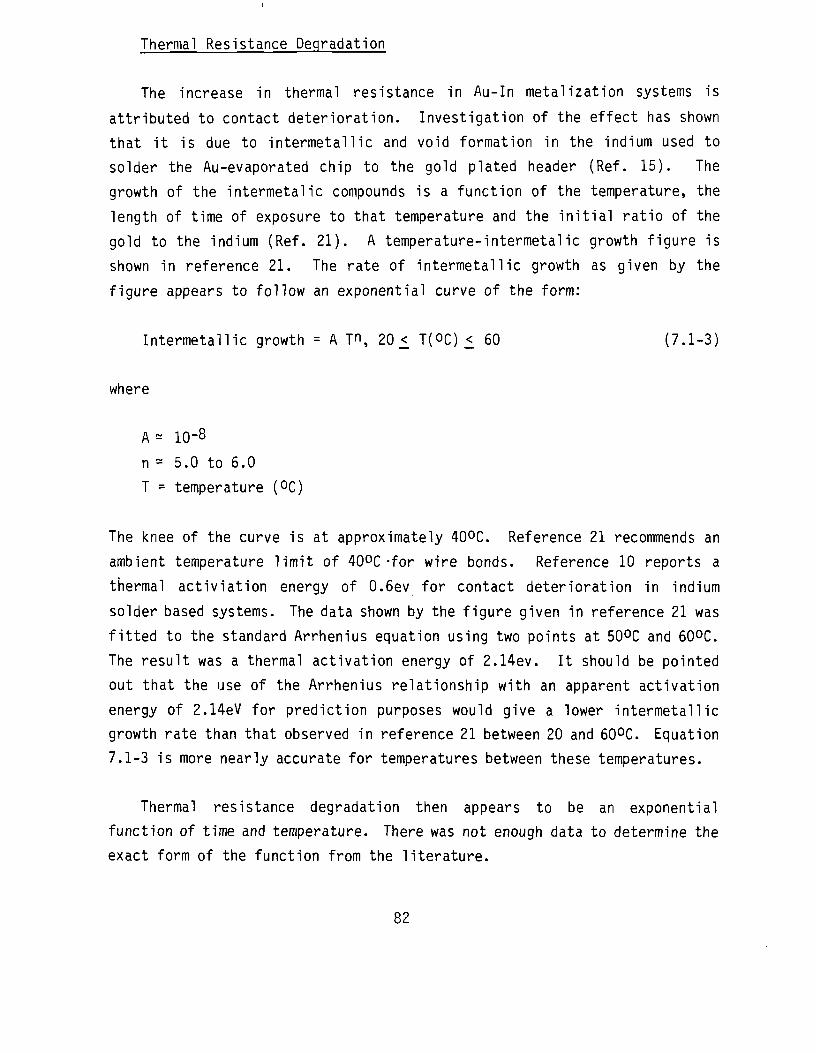
Thermal Resistance Degradation
The increase in thermal resistance in Au-In metalization systems is
attributed to contact deterioration. Investigation of the effect has shown
that it is due to intermetallie and void formation in the indium used to
solder the Au-evaporated chip to the gold plated header (Ref. 15). The
growth of the intermetalic compounds is a function of the temperature, the
length of time of exposure to that temperature and the initial ratio of the
gold to the indium (Ref. 21). A temperature-intermetal ic growth figure is
shown in reference 21. The rate of intermetal lie growth as given by the
figure appears to follow an exponential curve of the form:
Intermetallic growth = A T", 20 <_ T(oc) £ 60 (7.1-3)
where
A= 10-8
n = 5.0 to 6.0
T = temperature (°C)
The knee of the curve is at approximately 40°C. Reference 21 recommends an
ambient temperature limit of 40°C -for wire bonds. Reference 10 reports a
thermal activiation energy of 0.6ev for contact deterioration in indium
solder based systems. The data shown by the figure given in reference 21 was
fitted to the standard Arrhenius equation using two points at 50°C and 60°C.
The result was a thermal activation energy of 2.14ev. It should be pointed
out that the use of the Arrhenius relationship with an apparent activation
energy of 2.14eV for prediction purposes would give a lower intermetallic
growth rate than that observed in reference 21 between 20 and 60°C. Equation
7.1-3 is more nearly accurate for temperatures between these temperatures.
Thermal resistance degradation then appears to be an exponential
function of time and temperature. There was not enough data to determine the
exact form of the function from the literature.
82
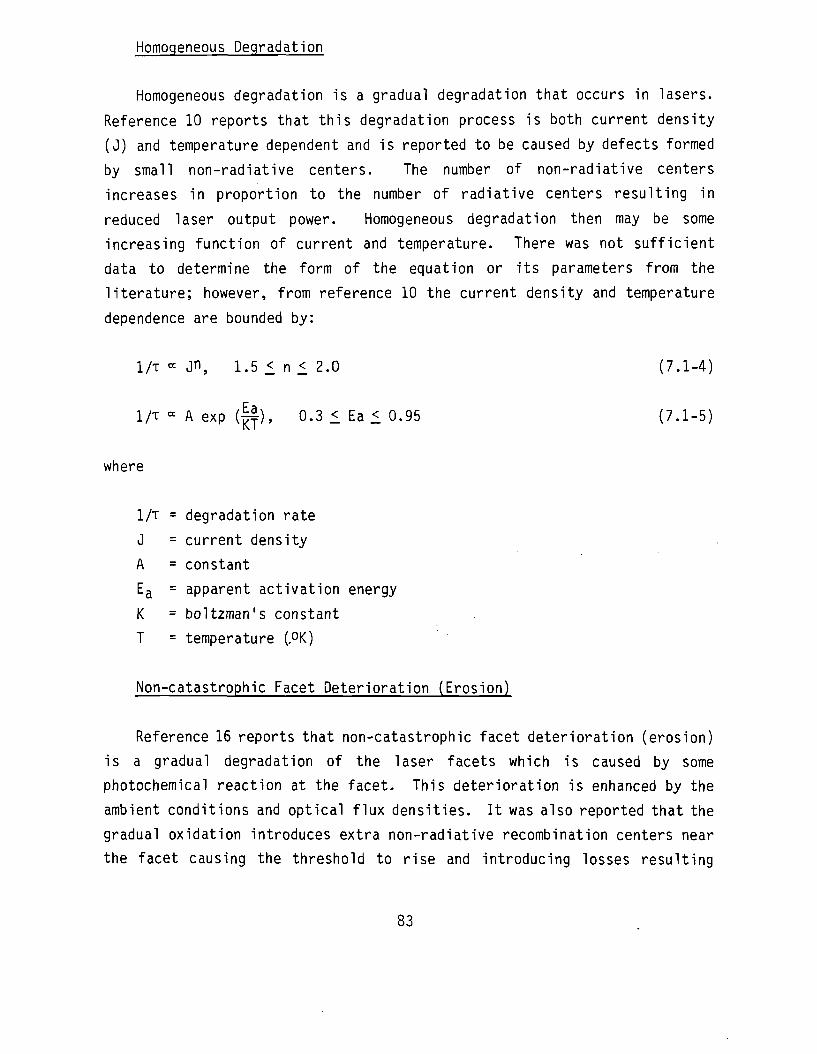
Homogeneous Degradation
Homogeneous degradation is a gradual degradation that occurs in lasers.
Reference 10 reports that this degradation process is both current density
(J) and temperature dependent and is reported to be caused by defects formed
by small non-radiative centers. The number of non-radiative centers
increases in proportion to the number of radiative centers resulting in
reduced laser output power. Homogeneous degradation then may be some
increasing function of current and temperature. There was not sufficient
data to determine the form of the equation or its parameters from the
literature; however, from reference 10 the current density and temperature
dependence are bounded by:
1/T « jn, 1.5 1 n £ 2.0 (7.1-4)
1/T * A exp (|Y)> 0.3 £ E a £0.95 (7.1-5)
where
1/T = degradation rate
J = current density
A = constant
E a = apparent activation energy
K = boltzman's constant
T = temperature (,°K)
Non-catastrophic Facet Deterioration (Erosion)
Reference 16 reports that non-catastrophic facet deterioration (erosion)
is a gradual degradation of the laser facets which is caused by some
photochemical reaction at the facet. This deterioration is enhanced by the
ambient conditions and optical flux densities. It was also reported that the
gradual oxidation introduces extra non-radiative recombination centers near
the facet causing the threshold to rise and introducing losses resulting
83

in a decrease in external quantum efficiency. Reference 10 reports that the
presence of oxygen or moisture in the ambient gases in contact with the facet
accelerates facet erosion, and that the facet erosion decreases the mirror
reflectivity and increases the non-radiative recombination rate at the
facets. Reference 10 also reports that facet erosion can be prevented by
coating the facet with a AI2O3 half-wave length thick film. A half-wave film
is used in order to leave the facet reflectively, and hence, the threshold
current unchanged. The application of a quarter-wavelength thick film would
decrease the reflectivity, and hence, increase the threshold current which
would accelerate other failure mechanisms. The coating is believed to
provide a moisture barrier. Reference 13 also reports that facet erosion is
a function of optical flux and ambient gases.
Non-catastrophic facet deterioration is some function of optical flux,
ambient and facet coating. Data were not available to determine the form of
the function or its parameters from the literature; however, references 13
and 15 report that a significant decrease in degradation occurs (>2X) when
facet coatings are utilized.
7.1.2.3 Functional Degradation Failure Mechanisms
Functional degradation failure mechanisms that have been documented fall
into three categories, Intensity Pulsations, Optical Frequency Shifts and
Emission Symmetry Changes.
Intensity Pulsations
Intensity pulsations are self sustained oscillations (SSOs) that have
been reported to occur at frequencies between 200MHZ and 3GHZ and at a
modulation depth approaching 100% (Ref. 9, 10, 16, 28). The onset of SSOs
could be detrimental if the laser was being used in a digital application.
The failure mechanisms that cause these SSOs have yet to be confirmed, but
there have been suggestions that either second order mode locking or
switching between two lateral filaments, or effects associated with
84

electron-photon interactions in the presence of non-uniform gain or loss, or
the effect of saturable absorbers in the active region are the cause (Ref.
16). The absorber may result from a localized region of lower population
inversion, caused by a region of non-radiative recombination, surface
recombination at the facets or the unpumped regions at the edges of the
stripe. The absorption in these areas will decrease with increasing pumping,
giving rise to a Q-switching effect (Ref. 16). One study (Ref. 9) reported
that SSOs were present in new devices and that the SSOs become enhanced by
forward-biased operation and/or elevated temperature. Data were not
available to derive an equation describing laser degradation or failure due
to SSOs. A second study (Ref. 28) reported that SSOs were present after
testing at elevated temperatures.
Several studies (Ref. 9, 10, 16, 28) have addressed this failure mode.
The distribution of devices that exhibited SSOs after lifetesting on a group
of AlGaAs double-heterostructure lasers (Ref. 28) is shown in Table 7.1-1:
TABLE 7.1-1: SSO DISTRIBUTION
Lasers that, degraded* during lifetest Lasers that did not degrade* after aging
4000 hour 521 hour 0 hour
STRONG SSO
10
4 0 0
WEAK SSO
8
3 0 0
NO SSO
12
5 5 18
TOTAL NO. OF DEVICES
30
12 5 18
TOTAL 14 11 40 65
*0ptical Power output degradation
Another study (Ref. 9) reported that 64 out of 103 samples (62%) exhibited
SSOs and that greather than 50% were converted from a stable laser to a
pulser during a 50-60 hour test. The data indicates that, at least for these
two batches of lasers, SSOs could be a major failure mode depending on the
85
circuit and application. The data also indicates that the onset of SSOs may
be time dependent and associated with other degradation mechanisms.
Optical Frequency Shifts and Light Intensity Changes
Optical frequency shifts are basically small alterations in the beam
direction and mode shape. These changes could be caused be minor internal
degradation which perturbs the cavity parameters in the junction plane
without significantly changing the efficiency (Ref. 10). Data were not
available to determine if operational parameters such as current and
temperature are activating influences, or to quantify the percentage of
devices that exhibit a frequency shift.
Emission symmetry changes are light intensity differences at the two
ends of the laser. The light intensity at one end is not the same as the
other and the difference varies with aging and drive current. One study
(Ref. 9) reported that 47 out of 95 (49%) of the samples exhibited an
emission symmetry change in the light polarized perpendicular to the
junction plane (TM) after accelerated testing. Reference 9 also reported
emission symmetry changes in the light polarized parallel to the junction
plane (TE), but the percentage of devices that exhibited a change was not
reported. Data were not available to determine if operational parameters
such as current and temperature are activating influences.
TM and TE emission symmetry changes and optical frequency shifts may
affect the performance of the laser in systems such as single-mode fiber
optical communications links and optical disks. The design engineer should
be aware of these devices characteristics, and design circuitry that are
tolerant of them.
86

7.1.3 Semiconductor Laser Reliability Prediction Procedure
The semiconductor laser failure rate is calculated using the following
equation:
Xp = XD TTE (7.1-6)
where
Xp = total device failure rate (F/lO&hours)
XQ = average degradation failure rate (F/lO^hours)
TTE = environmental factor (Table 7.1-2)
The failure rate prediction procedure is as follows:
STEP 1: Calculate the average failure rate
STEP 1A: Calculate the average optical power output degradation rate using
the following equation:
T p = T b X TTJ X TT J X TTQ X V f\ X TT p ( 7 . 1 - 7 )
where
Tp = semiconductor laser optical power output degradation rate (%/1000
hours)
Tb = base degradation rate (%/1000 hours) (Table 7.1-3)
Try = temperature factor
= exp , T = Case Temperature (°C)
where E = apparent activation energy/Boltzman's Constant (Table 7.1-3)
87

n is valid for +25°C < T < + 100°C
TTC = construction factor (Table 7.1-4)
TTA = application factor (Table 7.1-5)
TTp = pulsed duty cycle factor
^jpu lsed duty cycle (Table 7.1-6)
ITi = (forward peak current (ma))
TTJ is valid for 0 <_ I <_ 25 amps
STEP IB: Calculate the Mean life of the device by the following procedure:
1) Ps = rated optical power output (mw)
2) define required optical power output (PR)
3) calculate the allowable degradation (D) as follows:
D (%) - !s_ilR x 100 (7#1.8)
4) mean life (u) = D(%)/T P
STEP 1C: Calculate the average failure rate using:
X D = 1/u (F/106 hours) (7.1-9)
STEP 2: Calculate the average semiconductor laser failure rate using the
equation:
Xp = X D x TTE (F/1Q6 hours) (7.1-10)
88

TABLE 7.1-2: ENVIRONMENTAL MODE FACTORS TABLE 7.1-4: CONSTRUCTION FACTORS
Environment
GB GF GM Mp NSB Ns Nu NH NUU ARW AlC AIT AlB AIA AlF AUC ALIT AUB AUA AUF SF MFF MFA USL ML CL
TTE
1 2.4 7.8 7.7 3.7 5.7 11 12 13 17 2.5 3.5 3.5 5.5 8 3 5.5 5.5 8 10 1 7.8 11 23 26 450
Construction TTQ
Facet Coat or 1.0 Hermetic Package
No Facet Coat 3.3
TABLE 7.1-5: APPLICATION FACTOR
Application TTA
Variable Current 1.0 Source with optical feedback
Fixed Current Source 1.5
TABLE 7.1-6: PULSED DUTY CYCLE FACTOR
TABLE 7.1-3: DEGRADATION EQUATION PARAMETERS
Device Type E (Xb X105)
AlGaAs 4635 2.21 GaAs 4635 2.81 InGaAs/InGaAsP 5784 188
Duty Cycle
1.0 0.9 0.8 0.7 0.6 0.5 0.4 0.3 0.2 0.1
*TTF = 1 Jduty
•ftp*
1.00 0.95 0.90 0.85 0.75 0.70 0.65 0.55 0.45 0.30
cycle
89

7.1.4 Model Limitations
The procedure described in paragraph 7.1.3 applies to the following
device constructions:
AlGaAs DH Stripe
GaAs SH Stripe
InGaAs/InGaAsP DH Stripe
The models only apply if the optical flux density is less than 3MW/CM2.
The procedure does not address the functional failure modes - self-
sustained-oscillations (SSOs), TM & TE symmetry change and frequency shift.
An estimate of the expected percentage of devices that may exhibit two of
these degradation modes is:
Self-Sustained-Oscinations (SSOs) 53%
TM Symmetry Change 49%
As can be seen from the data, these two failure modes may occur in a large
percentage of the devices. It is impossible at this time to quantify their
impact on system reliability since they are not parameters that are specified
in the device data sheets, no definition of failure exists, and no field data
are available.
The temperature and drive current extremes that were available to derive
the factors TTJ and TTJ are given in Table 7.1-7.
TABLE 7.1-7: TEMPERATURE AND CURRENT LIMITS
Variable Upper Value Lower Value
Temperature + 100OC + 22°C
Drive Current 25 amps 50 ma
90

There were two data points at -35°C; however, these were not utilized to
derive the TTJ factor. The models are then limited to temperatures and
currents between the ranges given above.
The procedure assumes that the catastrophic failure rate and degradation
rate are constant.
7.1.5 Model Development
All of the data collected during this study effort were obtained from
either life tests or special research studies. With the exception of two
sources of data (Ref. 3, 21) all of the data were obtained from published
articles or manufacturer's product catalogs. Over 50 letters were written to
semiconductor laser manufacturers and researchers, and one trip was made to a
major semiconductor laser manufacturer to obtain reliability information and
data. No reliability data were obtained from any of these inquiries.
The data and information extracted from the literature are listed in
Table 7.1-8.
The approach to model development for semiconductor lasers was to
hypothesize a preliminary model form and general values for the model
parameters based on data and information extract id from the literature. The
life test data extracted from the literature was then used to develop
empirical estimates for the model parameters based on all of the available
data. The average degradation rate model was deemed necessary since
parameter degradation occurs early in the life of the device and the constant
hazard rate assumption over the life of the equipment may not be accurate.
The development of this model is presented in the following paragraphs.
91

TABLE 7 . 1 - 8 : TEST DATA
REF
2
e e e e e 10 10 10 10 13 13 14 17 17 19 19 22 22 22 23 23 23 23 23 23 23 23 1 6 3 3 3 3 9 9 15 15 15 15 18 18 IB 18 18 24 24 24 24 24 25 25 15 15 31 29 29 29 29 30 30 28 28 28 28 2b
DEVICE TYPE
(7)
Hi I! II II II 11 1 I I 1 1 II III II 11 1A IA IA IA IA I I I 1 I I I II VI X VI VI VI VI 11 11 IA IA IA IA X X X X X
VI IA VIIA VI1A V11A VIIA V11A VIIA I n IX I 1 1 I X X 1 I I 1
VIIA
CURRENT (Ma) (2)
260 160 160 160 V V 180 V V V c c V 170 C V V V V V 200 200 200 200 200 200 450 200
25,000 C
11,000 11,000 11.000 11.000
V V V V V V V 0 50 75 100 150 C C C C 150 100 C c V V V V V 130 195 V V V V 100
TEST TEMP F REG. ME AS.
(°C) (3) (6)
27 90 55 25 25 25 70 7D 70 22 22 22 55 70 70 18 18 90 90 24 100 90 80 70 60 22 22 22 27 70 22 65 -35
65 4-35 70 70 18 55 70 90 25 25 25 25 25 20 70 80 90 100 22 70 25 25 70 70 70 70 t 70 ( GO 50 70 70 70 -70 -S
NO. TESTED
6 11 1 4 4 20 40 40 7 24 8 I 72 10D 1 16 13 ---15 15 15 15 15 8 1 2 -. 63 9 9 9
103 95 -4 5 4 6 ----1 ----1 4 5 26 30 12 15 7 8 3 4 40 12 5 18 4
NO. FAILED
-----0 38 37 6 7 1 0 20 74 --------2 1 2 --0 0 0 0 64 47 _ ----------------18 0 0 0 0 --30 7 0 0 ~
TOTAL 0EV1CE (HOURS)
150,000 33.500 3,500 24.000 12,000 10,000 119,300 187,450 58,100 750.000 84,000 18,000
-450,506 10,000
----------
154,000 21,334 8,000
--
636,552 90,936 90,936 90,936 6,180 5,700
-16,000 20,000 16,000 12,000
500 500 25 10
4,500
------1.500 7,800
237,190 120.000 160,000 70,000 80,000 17.100 4,000
180,000 48,000 2,605
0 48,000
TEST LENGTH (HOURS)
25,000 4,500 3,500 6,000 3,000 500
10,000 10,000 16,000
>40,000 11.000
>18,000 10,000 14,500 10,000 25,000 25.000
-10.500
------
22,000 21.334 5,500
--
10,104 10,104 10,104 10,104
60 60
>30,000 4,000 4,000 4,000 2,000 500 500 500 500
4,500
----
12,000 12,000
300 300
11,500 10,000 10,000 10,000 10,000 5,700 1,000
10,000 4,000 521 0
12,000
DEGRADATION RATE C 1000 HOURS)
CURRENT
. 19.1 6.1 1.2 3.2 ----------0.7 0.6 8.0 15.0 2.0 39.2 32.2 10.2 3.7 1.5 -----------1.0 0.7 1.9 9.0 6.0 0
15.0 27.0 36.0
-----1.2
1.7 0.7 0.5 0.4 3.7 29.1
"
POWER
l.D
-----
26.3 18.2 14.0 0.6 0.9 6.8 12.5 11.1 2.5 ----------4.0 -
11.5
---------------0.7 ----3.2 1.1 7.7 13.5
--------- ( -1.4
HLDIA». LIIE (HOURS,
50.QUO 1.047 3,279 16,667 6,250
(1)10,929 1.900 2,747 3.571
80,000 55,550 7,353 4.000 4.500 20,000 28,571 33.333 2.500 1,333 10,000
510 621
1,961 5.405 13,333 77,000 12,500 4.000 4,348 11.000
(1)695,700 (1) 99,384 (!) 9S.3H4 (1) 99,384 (4) 97 (5) 121
20,000 28,571 10,526 2,222 3,333
-1,333 741 556
71,428 1,050 400 650 550
15,625 45,454 6.494 3,704 9,300 11.765 2C.571 40,000 50.00C 5.405 687
(4)6,000 (4)6.ES7
4)11)2.632
-35.714
NOTES:
(1 ) 601 Lower Confidence Level (2 ) V - Current va r ied to mainta in a set output
C - Current constant but magnitude is unknown (3 ) 1 - CW (100% duty cycle)
2 - 5KHZ, 200 ns pulses (0 .1S duty cyc le ) 3 - 500 HZ, 80 ns pulse (0 .0051 duty cyc le ) 4 - 10 MHZ, 20'. duty cycle w i th 901 threshold current bias 5 - 1 0 MHZ, 501 duty cycle w i th 90*. threshold current bias 6 - 1 0 MHZ, 50" duty cycle w i th SO", threshold current bias
(4 ) HT1F for s e l f sustained o s c i l l a t i o n s (5 ) MTTF for frequency s h i f t (6 ) L - La sing mode
5 - Spontaneous mode (LED) ( 7 ) 'A' a f t e r ROMAN Numerial indicates that presence or absence of f a c e t coat ing is unknown
92

7.1.5.1 Preliminary Model Development
The following preliminary failure rate model was developed entirely from
the data and information extracted from the sources listed in the references:
Degradation Rate:
T p = T b X TTC X TTE X TTF X TTA (7.1-11)
where
Tp = semiconductor laser optical power output degradation rate (%/1000
hours)
TTA = application factor
TTC = construction factor
TT£ = environmental factor
irp = duty cycle factor
Tb = AIn exp ill KT (7.1-12)
where
A = Constant
I = drive current
1.5 _< n_< 2.0
K = Boltzman's constant
T = Case temperature (°K)
E a = apparent activation energy
°-3l Ea± 1-1
The rationale for the adoption of the degradation rate model form and the
parameters included in the model is presented below.
93
A review of the literature disclosed that at least three of the failure
mechanisms associated with semiconductor lasers, dark line defects (DLDs),
dark spot defects (DSDs) and catastrophic facet damage, result in the rapid
degradation of the device; and that a high temperature burn-in in the order
of fifty to one hundred hours would eliminate most of the devices that would
fail because of these mechanisms. The review also disclosed that the
occurrence of DLDs and DSDs is a function of stresses that are induced by the
process materials and/or by the manufacturing process. Another failure
mechanism, ohmic contact degradation, has been found (reference 21) to be a
function of the bond materials. A fifth failure mechanism, facet erosion,
has been found to be a function of optical power density and the moisture or
oxygen content of the atmosphere in contact with the facet where both
increasing optical power density and the presence of oxygen or moisture
increases the degradation rate of the laser. A good oxygen and moisture
barrier, then, whether it is a facet coating or a hermetic package is
important for device reliability. Therefore, because of the reasons listed
above, a quality factor should be included in the failure rate model. There
are, however, at this time no defined quality levels for semiconductor
lasers. According to one semiconductor laser manufacturer, semiconductor
lasers are still custom devices and any testing or screening that is
performed varies considerably and is defined by the procurement
specification. Because there are no defined quality levels and because most
of the data collected are for non-packaged devices that were subjected to
routine testing, no quality level factors could be developed that are a
function of test or screen level.
Data were collected from several sources (reference 13, 15, 23) that
showed a correlation between laser performance and the presence or absence of
facet coatings. These data are as follows: Reference 13 shows a 7.6:1
improvement factor, reference 23 shows a 1.7:1 improvement factor and
reference 15 shows a 1.8:1 improvement factor. The geometric average of the
degradation rate given in these three references for AI2O3 facet coated
lasers and non-facet coated lasers is 2.3%/1000 hours and 6.6%/1000 hours
respectively which gives a ratio of 2.9 or approximately 3.0. The tests were
94

performed on non-packaged devices. Since the facet coat protects the laser
facet from the environment, the use of a hermetic package should provide
similar protection. Based on these data the construction factors (TTC) shown
in Table 7.1-9 were assumed.
TABLE 7.1-9: CONSTRUCTION FACTORS
Construction TTC
Lower* 1.0
Plastic,** with AI2O3 Facet Coating 1.0
Plastic,** no Facet Coating 3.0
*Applies to all hermetic packaged devices
**Applies to all non-hermetic packaged devices
A review of the literature also disclosed that, except for the
degradation that occurs because of facet erosion, facet damage, and to some
extent DLDs and DSDs, the failure mechanisms and their activating influences
that impact semiconductor lasers are the same as those that impact LEDs.
These similarities; plus the fact that no field failure experience data were
available to develop separate environmental factors for semiconductor
lasers, led to the assumption that the environmental factors for Opto
electronic Devices given in MIL-HDBK-217D would adequately account for the
reliability impact of environment on semiconductor lasers.
The duty cycle factor (TTP) is based on work performed by Yoshida et.al
(reference 29) where they showed that the laser diode degradation rate was
proportional to duty cycle, operating current and temperature. The duty
cycle function was given as:
Degradation rate « (duty cycle)0«5 (7.1-13)
This relationship was based on three data points; 20, 50 and 100% duty cycle,
where the relative degradation rate, which is defined as the pulsed operating
95

degradation rate divided by the CW operating degradation rate, versus duty
cycle measured is given in Table 7.1-10.
TABLE 7.1-10: DUTY CYCLE DEGRADATION RATES
Relative Degradation Rate
Lower Bound
0.16
0.17
Measured Point Estimate
1.0
0.38
0.27
Upper Bound
0.96
0.45
Calculated
1.0
0.71
0.45
Duty Cycle
100
50
20
The measured values shown above are approximations because they were
extracted from a figure. The confidence limit used to generate the upper and
lower bounds was not given. Based on these data the duty cycle factors SHOWN
IN Table 7.1-11 were assumed.
TABLE 7.1-11: ASSUMED DUTY CYCLE FACTORS
Duty Cycle {%) irp
100 1.0
90 0.95
80 0.90
70 0.85
60 0.75
50 0.70
40 0.65
30 0.55
20 0.45
10 0.30
The application factor (TTA) is based on work performed by Ettenberg,
et.al. (Ref. 10) where one of their studies was a comparison of laser
96

lifetime considering two definitions of failure; the first when the laser
drops to half its initial output at constant current and the second where the
laser can no longer emit 1.25mw at the 70°C heat sink temperature. The tests
were conducted on 40 low-threshold (=50ma) oxide-defined stripe lasers. The
operating conditions were initial power output -4mw CW at 70°C heat sink
temperature. The median times-to-failure were:
Time to 50% Power Degradation - 1900 hours
Time to -1.25 mw output - 3800 hours
If a linear degradation rate is assumed, the degradation rates for the two
failure definitions are:
Time to 50% Power Degradation = ((4-2)/4)/1000 hours or 26.3%/1000 hours Time to <1.25 mw output = ((4-1.25)/4)/3800 hours or 18.1%/1000 hours
These two failure definitions correspond to two possible laser circuit
designs -constant current and variable current with an optical feedback
circuit. Based on the data given above the two application faccors shown in
Table 7.1-12 were assumed.
TABLE 7.1-12: APPLICATION FACTORS
Application T\/\ Variable Current W Optical Feedback 1.0 Constant Current 1.5
Of course, if optical feedback is employed, additional external components would be required for the design. The application factor can then be used by the circuit designer to perform reliability trade-off studies.
The base degradation rate factor, t^, has been found to be a function of
temperature, drive current, optical power density, laser construction and
definition of failure. The greatest difficulties encountered during the
97
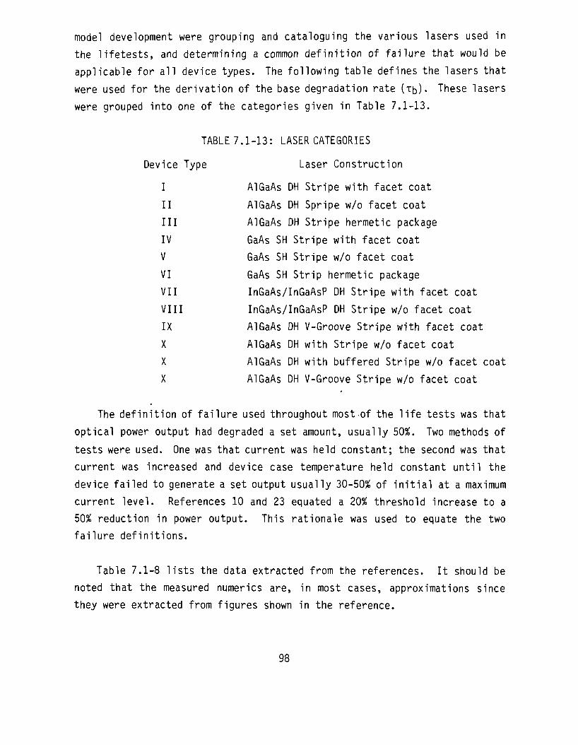
model development were grouping and cataloguing the various lasers used in
the lifetests, and determining a common definition of failure that would be
applicable for all device types. The following table defines the lasers that
were used for the derivation of the base degradation rate (xb). These lasers
were grouped into one of the categories given in Table 7.1-13.
TABLE 7.1-13: LASER CATEGORIES
Device Type Laser Construction
I AlGaAs DH Stripe with facet coat
II AlGaAs DH Spripe w/o facet coat
III AlGaAs DH Stripe hermetic package
IV GaAs SH Stripe with facet coat
V GaAs SH Stripe w/o facet coat
VI GaAs SH Strip hermetic package
VII InGaAs/InGaAsP DH Stripe with facet coat
VIII InGaAs/InGaAsP DH Stripe w/o facet coat
IX AlGaAs DH V-Groove Stripe with facet coat
X AlGaAs DH with Stripe w/o facet coat
X AlGaAs DH with buffered Stripe w/o facet coat
X AlGaAs DH V-Groove Stripe w/o facet coat
The definition of failure used throughout most of the life tests was that
optical power output had degraded a set amount, usually 50%. Two methods of
tests were used. One was that current was held constant; the second was that
current was increased and device case temperature held constant until the
device failed to generate a set output usually 30-50% of initial at a maximum
current level. References 10 and 23 equated a 20% threshold increase to a
50% reduction in power output. This rationale was used to equate the two
failure definitions.
Table 7.1-8 lists the data extracted from the references. It should be
noted that the measured numerics are, in most cases, approximations since
they were extracted from figures shown in the reference.
98
The degradation rate model developed herein can be used to predict the
degradation rate of the laser due to facet degradation, contact
deterioration, dark line defects, dark spot defects and homogeneous
degradation. It will not predict the expected number of failures due to
self-sustained oscillations and/or frequency shifts or waveshape changes.
The following paragraphs discuss the magnitude of these last two failure
modes.
Paoli (reference 9) conducted experiments that showed that 62% of a group
of laser diodes, which were initially stable, exhibted pulsations and that
49% of the same group of laser diodes exhibited a change in the emission
symmetry of the light polarized perpendicular to the junction plane (TM)
following a 50-60 hour, 70°C burn-in. The actual test data showed that 64
out of 103 devices exhibited pulsations after the burn-in. The literature
also stated that there were many other devices that exhibited pulsations
prior to the burn-in. The exact number was not given, but the percentages
were 16, 30, 24 and 5% from wafers A, B, C and D respectively. If the number
of samples from wafers A, B, C and D subjected to the burn-in were increased
by the percentages given, then the actual number of failures would be 88
failures out of 127 devices. Relating this to a failure rate based on the
50-60 hour burn-in gives 69.3%/55 hour or 12,600F/106 hours. The x2 80%
confidence limits about this estimate are 11,024F/106 hours and 14,316F/106
hours.
The actual test data showed that 47 out of 95 devices exhibited a TM
Emission Symmetry change during the 50-60 hour burn-in. This corresponds to
a 49.5%/55 hour or 9,000F/106 hour failure rate. The 80% confidence limits
about this estimate are 7,560F/106 hour and 10,718F/106 hours.
The results of this study showed that a large percentage of devices
exhibited these failure modes during the first 50 hours of a high temperature
burn-in, and, therefore, that a 70°C, 60-hour burn-in and screen would
eliminate a large portion of the devices that could possibly fail due to
these failure modes.
99

Another study (reference 28) also showed that SSOs are a major failure
mode; however, this study indicated that a longer burn-in (>500 hours) may be
required to screen out the susceptible devices. The data shown in Table 7.1-
14 were generated during the study.
TABLE 7.1-14: SSO DISTRIBUTION
Following these STRONG WEAK NO TOTAL
test Conditions SSO SSO SSO
Degraded (1) 10 8 12 30
Aged 4000 hours (2) 4 3 5 12
Aged 521 hours (2) 0 0 5 5
No Aging 0 0 18 18
Total 14 11 40 65
Notes: 1) Lasers that had failed to generate a minimum stimulated emission at 70°C during a 70°C life test but which continued to operate CW at room temperature.
2) Aging was at 70°C with no appreciable degradation.
As can be seen the percentage of lasers that exhibited SSOs is approximately
the same for the degraded and the aged 4000 hour devices (60% and 58%).
Based on the data given above, it is obvious that SSOs and TM emission
symmetry changes are major failure modes; however, insufficient data were
available to allow for their incorporation into the failure rate prediction
model. It is proposed that the model be defined as excluding these failure
modes. It is recommended that, if these failure modes could result in a
circuit failure, that the devices be screened to eliminate any devices
exhibiting SSOs and that the screen include a 70°C burn-in of at least 60
hours duration. As was mentioned previously, data were not available to
derive a factor for the predicton model that would account for these failure
modes. This was because, except for the two references listed above, the
100

life tests did not address these failure modes, and the data given in these
two references were somewhat contradictory.
The data shown in Table 7.1-15 is given to aid the designer in assigning
a failure numeric for these failure modes.
TABLE 7.1-15: FUNCTIONAL DEGRADATION MODE DISTRIBUTION
Failure Mode Ref Percentage of devices that failed during: 60 hour 521 hour 4000 hour
70OC Screen 70OC Screen 70OC Screen
TM Emission Symmetry 9 49.3 — — change
SSOs 9 69.3
SSOs 28 — 0.0 58.3
This failure numeric would be an additive factor in that it would be
considered along with the failure rate generated by the failure rate
prediction model. If the limited 4000 hour data were used, an average
failure rate of 58.3%/4000 hours or 146F/106hours would be added to the
failure rate generated"by the failure rate prediction model to account for
the SSO failure mode. By comparison, the failure rate generated by the
prediction model for a AlGaAs facet coated DH stripe laser used in a ground,
fixed environment at 55°C with a fixed dc current source at lOOma and the
allowable degradation is 50% is 266 F/106 hours. It should be noted again
that the potential contribution of this failure mode to the device failure
rate is significant, but that it may be controllable by the circuit design.
7.1.5.2 Model Refinement
Model refinement consisted in fitting the data shown in Table 7.1-8 to
the preliminary model forms. The regression technique described in Section
3.1 was used to fit the data.
101

Due to the limited amount of data, it was necessary to fix the parameter
E a at 0.4ev for GaAs and AlGaAs devices. The value of 0.4ev for E a was chosen
for GaAs and AlGaAs devices since it agrees with the results obtained by
Ritchie et. al. (Ref. 8) when both the Arrhenius relationship and current
are considered in the degradation model with the current factor normalized
out.
The data in Table 7.1-8 for device types, I, II, III, IV, V, VI, IX, and X
were regressed (regression No. 1) to develop the application factor TT/\, the
duty cycle factor (frp), the construction factor (TTC) and current factor (In).
The data for device types I, II, III, IV, V and VI were then regressed with
degradation rate as the dependent variable (regression No. 2) to develop the
base degradation rate factor (xb) for the AlGaAs and GaAs devices. The data
for device types VII and VIII were regressed (regression No. 3) to develop
the temperature relationship (Ea) and base degradation rate (xb) for the
InGaAs/InGaAsP devices. In the second and third regressions the factors TT/\,
TTF, TTC and In were fixed at the values derived in the first regression. The
purpose of the second and third regressions was to obtain the temperature
relationship since the literature (Ref. 10, 16, 20) indicated that
InGaAs/InGaAsP devices were more temperature sensitive than the GaAs and
AlGaAs devices.
The results of the regression were:
Tp = Tb X 7TJ X I n X 7TC X 7TA X TTp (7 .1 -14 )
where
Tp = semiconductor laser degradation rate (%/1000 hours)
Tb = base degradation rate (%/1000 hours)
TTT = temperature factor
exp -E
(T + 273) , T = Case Temp (°C), E = Ea/K
102

In = current (ma)
TTC = construction factor
TTA = application factor
TTF = duty cycle factor
= Fm
and with the constants as shown in Table 7.1-16 where the standard error
statistic was used to calculate confidence intervals about the derived
factors where possible.
TABLE 7.1-16: MODEL CONSTANTS
(A) TTC, Construction Factor
Construction
Facet Coat or Hermetic
W/0 Facet Coat
L 20% Limit
—
2.1
TTQ
PT EST
1.0 3.3
U 80% Limit
—
5.1
(B) TT/\, Application Factor
Application
Variable Current Source
with optical feedback
Fixed Current Source
Device Type
AlGaAs
GaAs
InGaAs/InGaAsP
(C)
L 20% Limit
—
0.90
Tq, Current Factor
L 20% Limit
0.12
0.12
0.12
*A PT EST
1.0
1.5
n PT EST
0.68
0.68
0.68
U 80% Limit
—
2.44
U 80% Limit
1.23
1.23
1.23
103

(D) Tb, Base Degradation Rate
Device Type ?b (X 105)
L 20% Limit PT EST U 80% Limit
AlGaAs -- 1.534
GaAs 1.095 1.952 3.481
InGaAs/InGaAsP -- 130.9
(E) Try, Temperature Factor
Device Type E*
L 20% Limit PT EST U 80% Limit
AlGaAs -- -4635
GaAs — -4635
InGaAs/InGaAsP -11390 -5784 -3687
* E = Apparent Activation Energy (EA)/Boltzman's constant (8.63 X 10~5)
(F) TTF, Duty Cycle Factor
m
L 20% Limit PT EST U 80% Limit
0.15 0.50 0.84
In order to derive a prediction model for a non-constant failure rate
device, an expression for the hazard function (in time) is required. For
practical purposes, it is required to express this as a cumulative average
over time; i.e., . J h(u) du, where h(u) is the hazard function and u a dummy
variable for integration.
We require an expression for
H(t) = \ ^h(u) du (7.1-16)
where h(u) = 1 . p(u)
104

and where f(u) is the failure (probability) density function and F(u) is the
associated cumulative density function.
So, for example, if f(u) is exponential,
h(u) =
X e - ^ e-Xu
so, H(t) =
Xe-Xu
1 _ (l-e-Xu)
X, as expected
(7.1-17)
Xt f- = X, again as expected.
However if the p.d.f. is lognormal,
1 i .In ii _ •,,. 2 f(u)
2TT a u is /In u - \i\ e-% ( (7.1-18)
where u and a are respectively the mean and standard deviation of the
associated normal distribution of In u;
then
»(*)-i lr IM. 1 - UCf(v) dv
du (7.1-19)
where v i s a second dummy variable of integration
Clearly, solution of 7.1-19 will be analytically tedious, and probably
impossible (given the difficulty of solving even the regular normal
integral).
Weibull approximation
The similar shapes of the lognormal and Weibull over certain ranges of a
and B, suggest that the readily soluble Weibull hazard may be appropriate.
This approach was investigated. The approach is discussed in the following
105

paragraphs. The data given in Table 7.1-17 were available with times-to-
failure, median life(u) and standard deviation (a). Table 7.1-17 also lists
the Weibull and lognormal parameters for the data sets.
TABLE 7.1-17: WEIBULL AND LOGNORMAL PARAMETERS COMPARISONS
Ref
10 10(1) 10(1) 14 17 19 31 31
Notes: (1) Same devices with different failure criteria.
The data were graphed on Weibull probability paper giving the Weibull
estimates for characteristic life (0) and slope (B) shown above. The
Kolmogorov-Smirnov (K-S) test described in Section 3.1 was used on the data
given above to determine if the Weibull slope was significantly different
from 1.0. The results of the test are given in Table 7.1-18.
TABLE 7.1-18: K-S TEST RESULTS
Log Normal
y
80000 1900 3800
40000 4500 74000 8800 11000
Parameters
a
15500 550 1250 2000 800
22000 1650 4450
Weibull
e
90000 3000 5800
33500 5000
105000 13000 13500
Parameters
B
1.15 1.05 1.10 0.65 0.95 1.40 0.80 1.50
Ref
10 10 10 14 17 19 31 31
No. of Failures
7 37 38 22 74 15 9 9
Max Dev
n'mum nation
.04
.14
.06
.21
.05
.27
.10
.10
K-S; -S ig'
Statistic iificance
.40
.18
.17
.23
.12
.28
.36
.36
(0. Leve
2 Jl)
Conclusion
No Difference No Difference No Difference No Difference No Difference No Difference No Difference No Difference
106

Based on the results of the K-S test, it was assumed that the failure
distribution of semiconductor laser could be described by a Weibull slope of
1.0.
The degradation rate equation, 7.1-14 described previously, was derived
from the time to 50% failure (median life) of the devices. The Weibull
Characteristic life (0) is the time to 63% failure. The median life estimate
was converted to a characteristic life estimate by revising the base
degradation rate (T^) constant. The technique used and the revision factor
is given below:
Given: T = time to 50% failures
F(t) = 1 - exp -(t/0)
0 = time to 63% failures
B = 1.0
t = T = time to 50% failures
(7.1-20)
Then: .5 = 1 - e
- .~t/0
-T/0
or: 0 = 1.44 T (7.1-21)
The following (average Weibull hazard rate) equation was then used to
derive an estimate of the failure rate:
T b-1 lavg (7.1-22)
where
T = operating time
b = Weibull slope
0 = Characteristic life
107
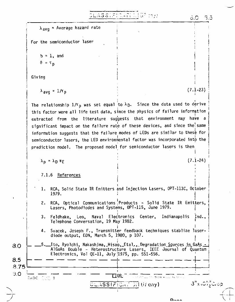
.0
.5
.75
.0
X a Vg = Average hazard rate j
For the semiconductor laser J ! i
b = 1, and j j 9 = T P i |
i Giving j
Xavg = lAp | (7-H3)
The relationship 1 A D was set equal to * D - Since the data used to derive ; 1 ' I
this factor were all life test data, since the physics of failure information
extracted from the literature suggests that environment may have a
significant impact on the failure rate of these devices, and since the! same
information suggests that the failure modes of LEDs are similar to these for
semiconductor lasers, the LED environmental factor was incorporated into the
prediction model. The proposed model for semiconductor lasers is then ; i
Xn = X D TT£ ! (7.1-24) 1 ; i 7.1.6 References ,
\ !
I 1. RCA, Solid State IR Emitters and Injection Lasers, 0PT-113C, October
1979. .' | 2. RCA, Optical Communications Products - Solid State IR Emitters,
Lasers, Photodiodes and Systems, OPT-115, June 1979. |
3. Feldhake, Leo, Naval Electronics Center, Indianapolis Ind., Telephone Conversation, 19 May 1982. '
i ! 4. Svacek, Joseph F., Transmitter feedback techniques stablize laser-
diode output, EDN, March 5, 1980, p 107.
5. I t o , Ryolchi, Nakashima,JHsap,Jital.,.,,Degradati.onJ>gur_ces JiLGaAs_2_j AlGaAs Double - Heterostructure Lasers, IEEE Journal of Quantum j Electronics, Vol QE-11, July|l975, pp. 551-556.
4-•+ •
TADC T2Q& H ^ i . . ) , ,
CL.ASS I F\ C.-s • >i 1 Ur any) 3 x ^ / , C i
O / - . ^ n
6. Wolk, Claus, Gottsmann, Hartmut, etal., Criteria for Designing V-Groove Lasers, IEEE Journal of Quantum Electronics, Vol. QE-17, No. 5, May 1981, pp. 756-758.
7. Hwang, C.J. and Svacek, Joseph S., Long lived diode lasers, Laser Focus, June 1979.
8. Ritchie, S., Godfrey, R.F., etal., The temperature dependence of degradation mechanisms in long-lived (GaAl) As DH lasers, Journal of Applied Physics, June 1978, pp. 3127-3132.
9. Paoli, Thomas L., Changes in the Optical Properties of CW (AlGa)As Junction Lasers During Accelerated Aging, IEEE Journal of Quantum Electronics, Vol QE-113, May 1977, pp. 351-359.
10. Ettenberg, Michael and Kressel, Henry, The Reliability of (AlGa)As CW Laser Diodes, IEEE Journal of Quantum Electronics, Vol. QE-16, No. 2., February 1980, pp. 186-196.
11. DeLoach Jr., B.C., Hakki, B.W., etal., Degradation of CW GaAs Double-Heterojunction Lasers at 300K, Proceedings of IEEE, Vol. 61, July 1973, pp. 1042-1044.
12. Barnes, C.E., Neutron Damage in Epitaxial GaAs Laser Diodes, Journal of Applied Physics, Vol. 42, No. 1, April 1971, pp. 1941-1949.
13. Ladany, I., Ettenberg, M., etal., AI2O3 half-wave films for long-life CW lasers, Applied Physics Letters, Vol. 30, January 1977, pp. 87-88.
14. Thompson, Alan, The Reliability of a Practical Gai_xAlxAs Laser Device, IEEE Journal of Quantum Electronics, Vol. QE-15, No. 1, January 1979, pp. 11-13.
15. Newman, D.H. and Ritchie, S., Degradation Pnenomena in Gallium Aluminium Arsenide Stripe Geometry Lasers, Cqechoslovak Journal of Physics, Vol. B30, 1980, pp. 336-344.
16. Newman, D.H. and Ritchie, S. Reliability and Degradation, Chapter 6, Reliability and degradation of lasers and LEDs, John Wiley and Sons, 1981, pp. 301-361.
17. Hartman, R.L., Schumaker, N.E. and Dixon, R.W., Continuously Operated (Al, Ga) As double-heterostructure lasers with 70OC lifetimes as long as two years, Applied Physics Letters, Vol. 31, December 1977, pp. 756-759.
18. Kobayashi, Takeshi and Furukawa, Yoshitaka, Recombination Enhanced Annealing Effect in AlGaAs/GaAs Remote Junction Heterostructure Lasers, IEEE Journal of Quantum Electronics, Vol. QE-15, No. 8, August 1979, pp. 674-684.
109

19. Kirkby, P.A. and Cox, A.A., GaAs Lasers - A Family of Laser Structures Emerging for New Applications, Microelectronics Reliability Vol. 19, 1980, pp. 633-644.
20. Yamakoshi, S., Abe, Masayaki, etal., Reliability of High Radiance InGaAsP/InP LEDs Operating in the 1.2-1.3um Wavelength, IEEE Journal of Quantum Electronics, Vol. QE-17, No. 2, February 1981, pp. 167-173.
21. Goddard Space Flight Center, Product Assurance Briefs, PAB No. 82-01, March 31, 1982.
22. Robertson, M.J., Wakefield, B. and Hutchinson, P., Strain-related degradation phenomena in long-lived GaAlAs stripe lasers, Journal of Applied Physics, Vol. 52, No. 7, July 1981, pp. 4462-4466.
23. Kressel, H., Ettenberg, M. and Ladany, I., Accelerated step-temperature aging of AlxGai_x As heterojunction laser diodes, Applied Physics Letters, Vol. 32, March 1978, pp. 305-308.
24. Olsen, G.H., Nuese, C.J. and Ettenberg, M., Reliability of Vapor-Grown InGaAs and InGaAsP Heterojunction Laser Structures, IEEE Journal of Quantum Electronics, Vol. QE-15, No. 8, August 1979, pp. 688-693.
25. Olsen, G.H., InGaAsP laser Diodes, SPIE, Vol. 224, Fiber Optics for Communications and Control, 1980, pp. 113-121.
26. Botez, D. and Herskowitz, G.J., Components for Optical Communications Systems: A Review, Proceedings of the IEEE, Vol. 68, No. 6, June 1980, pp. 689-731.
27. Ettenberg, M., A Statistical study of the reliability of oxide-defined stripe CW lasers of (AlGa) As, Journal of Applied Physics, Vol. 50, No. 3, March 1979, pp. 1195-1202.
28. Channin, D.J., Ettenberg, M. and Kressel, H., Self-sustained oscillations in (AlGa)As oxide-defined stripe lasers, Journal of Applied Physics, Vol. 50, No. 11, November 1979, pp. 6700-6706.
29. Yoshida, Jun-Ichi, etal., Degradation Behavior of AlGaAs Double-Heterostructure Laser Diodes Aged Under Pulsed Operating Conditions, IEEE Journal of Quantum Electronics, Vol. QE-18, No. 5, May 1982, pp. 879-884.
30. Shimizu, Hirokazu, etal., Improvement in Operation Lives of GaAlAs Visable Lasers by Introducing GaAlAs Buffer Layers, IEEE Journal of Quantum Electronics, Vol. QE-17, No. 5, May 1981, pp. 763-767.
110

31. Arnold, Gunther, etal., Long-Term Behavior of V-Groove Lasers at Elevated Temperature, IEEE Journal of Quantum Electronics, Vol. QE-17, No. 5, May 1981, pp. 759-762.
7.2 Helium-Cadmium Lasers
7.2.1 Device Construction
The helium-cadi urn (He-Cd) laser is a low current, high voltage,
continuous wave, gas discharge laser. The laser exits a single blue line at
442 nm. Typical tube currents are in the 50-100ma region, and typical tube
voltages are in the 1.5KV range. Current density in the bore is =4A/CM2,
dissipation -3W/CM of length and gas pressure are =6 Torr. Power outputs
range from 5 to 50 mw. Total tube dissipation is quite low and units are
cooled by natural convection (Ref 1). The construction of a He-Cd laser tube
is shown in Figure 7.2-1. The primary uses of He-Cd lasers are commercial
recorders, reprographics, spectroscopy and Q/A scanning.
CONDENSER
/ * BREWSTER WINDOW
"V
He BOTTLE
\ ANODE
PIN
lO)
LJL/f COLD TRAP
CADMIUM RESERVOIR
CATHODE
FIGURE 7.2-1: HELIUM-CADMIUM LASER TUBE
Principle design considerations relating to the lifetime of the device
include (Ref 1):
o Minimizing He gas cleanup via depositing Cd metal and cathode sputtering,
111
o Maintaining a uniform mix of He gas and Cd vapor in the discharge,
o Protection of Brewster windows from condensing Cd, and
o Blockage of the optical path by deposits of Cd.
7.2.2 Failure Modes/Mechanisms
The primary failure modes and associated mechanisms of a He-Cd laser are:
o Power output degradation
Helium gas loss due to
o cathode sputtering o burial of He under condensing Cd o wall diffusion
Cadmium depletion from the reservior
o normal vaporization o cataphoretic transport down the bore to the condenser
Discharge contamination by impure gases resulting from materials out gassing or incomplete processing
Growth of Cd deposits into the optical beam in the vicinity of the condenser
0
0
Filament Failure
Rapid gas loss
Glass Crack Seal Leak
o Resonator/Beam Misalignment
Failure mechanism distributions reported by two data sources are
presented in Table 7.2-1 along with a distribution based on the combined
results.
112
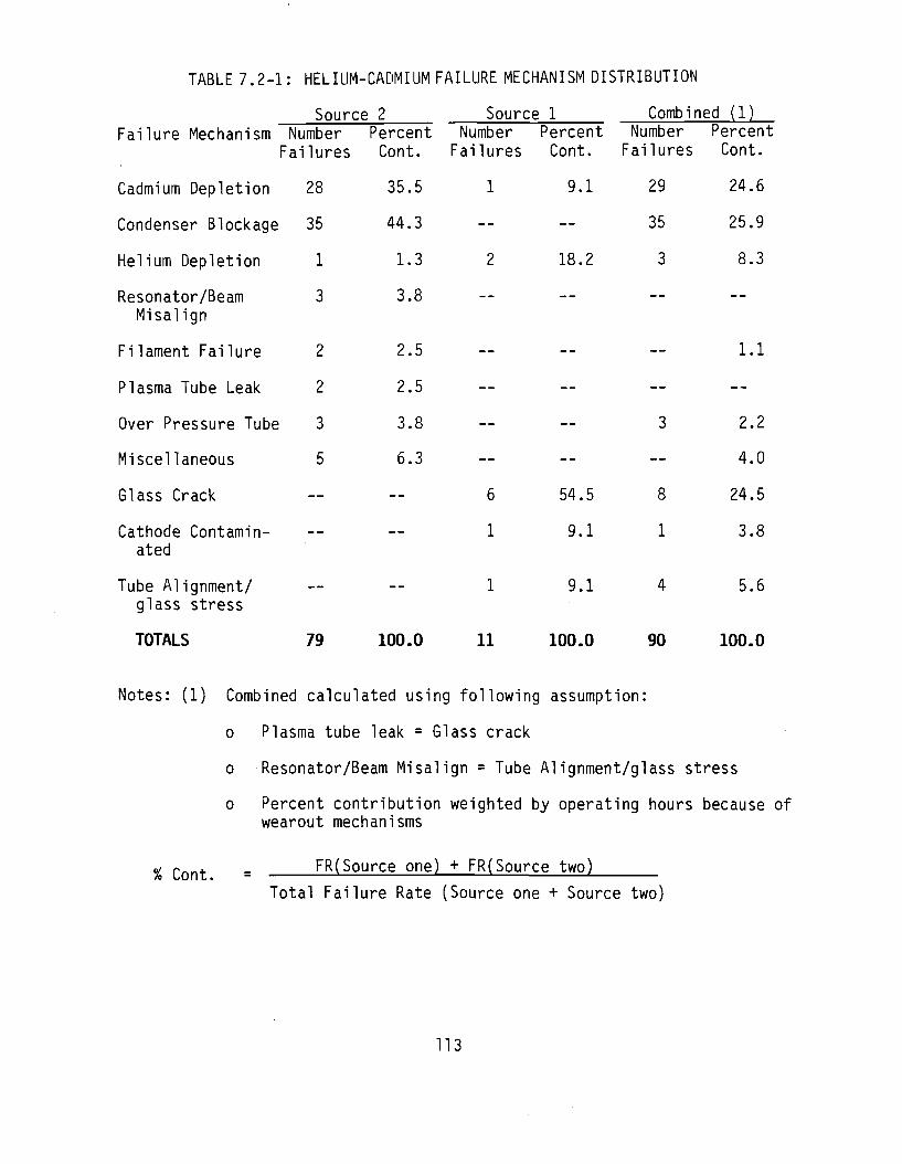
TABLE 7.2-1: HELIUM-CADMIUM FAILURE MECHANISM DISTRIBUTION
Source 2 Source 1 Combined (1) Failure Mechanism Number Percent Number Percent Number Percent
Failures Cont. Failures Cont. Failures Cont.
Cadmium Depletion 28 35.5 1 9.1 29 24.6
Condenser Blockage 35 44.3 — — 35 25.9
Helium Depletion 1 1.3 2 18.2 3 8.3
Resonator/Beam 3 3.8 Misalign
Filament Failure 2 2.5 -- -- -- 1.1
Plasma Tube Leak 2 2.5
Over Pressure Tube 3 3.8 -- -- 3 2.2
Miscellaneous 5 6.3 -- -- -- 4.0
Glass Crack — — 6 54.5 8 24.5
Cathode Contamin- -- — 1 9.1 1 3.8 ated
Tube Alignment/ — — 1 9.1 4 5.6 glass stress
TOTALS 79 100.0 11 100.0 90 100.0
Notes: (1) Combined calculated using following assumption:
o Plasma tube leak = Glass crack
o Resonator/Beam Misalign = Tube Alignment/glass stress
o Percent contribution weighted by operating hours because of wearout mechanisms
* Q t _ FR(Source one) + FR(Source two)
Total Failure Rate (Source one + Source two)
113

7.2.3 Helium-Cadmium Failure Rate Model
*• He-Cd = * E *• MEDIA + * E x COUPLING
where
^He-Cd = helium-cadmium laser failure rate in f/106 operating hours.
IT E = environmental application factor, determined from Table 7.2-2.
^MEDIA = failure rate contribution of the lasing media.
= 228 failures/106 operating hours.
^•COUPLING = failure rate contribution of the laser coupling hardware. = 0.1 failures/106 operating hours.
It should be noted that the helium-cadmium laser failure rate prediction
model can be simplified and rewritten as:
xHe-Cd = 228.1 TT E
7.2.4 Model Development
The approach utilized was to hypothesize a model form based on the theory
of operation and physics of failure of the laser. Data were collected;
however, there was insufficient data to support this preliminary model form.
It was then considered appropriate to adopt the model form of the current
Helium-Neon laser. This is a realistic assumption because of the similarity
in construction and application between the two laser types. A unique media
parameter was then derived for the helium-cadium laser.
The following preliminary model was hypothesized:
xHe-Cd = xc + xd
114

TABLE 7.2-2: ENVIRONMENTAL MODE FACTORS
Environment
GB GF GM Mp
NSB Ns
Ny NH
NUU ARW
AlC AIT
AlB
*E 0.2
1
5
2.3
1.1 5
5
3.6
3.9 5.2
3
3
6.5
Environment
AlA
AlF
AUC AUT AUB
AUA
AUF
SF
MFF
MFA
USL ML
CL
E 5
7
6
5
10
8
10
0.2
2.4
3.3
7.0
8 N/A
where
^He-Cd = helium-cadmium laser failure rate in failures/10^ operating
hours.
\- = random failure rate contribution (F/106 hours)
\j = average degradation failure rate contribution (F/10^ hours)
where
X, = /T 1 _ , f2 h(t) dt
(T2 - Ti) Tl
T2 - T]_ = operate time or replacement interval
h(t) = the hazard rate function
Empirical data were received from two proprietary sources. The source 1
data shown in Table 7.2-3 are life test times-to-failure on 18 devices.
115

TABLE 7.2-3: LIFE TEST TIME-TO-FAILURE
Device Time-To-Failure (hours)
1
2
3
4
5
6
7
8
9
10
11
500
1000
2400
2840
2908
3200
4190
4196
4300
4500
5100
12-18 Did not fail
Total Hours 58198
The definition of failure used was when the power output of the tube dropped
to less than 50% of specified power. The tubes tested were all nominally
10MW specified power. These laser tubes are terminated in Brewster windows.
Two cavity mirrors are used; a flat high reflector and a 60cm (curvature)
output coupler. No failures were recorded on the optics. Six of the
failures (Pin seal failures (glass crack)) were identified as attributed to
manufacturing errors (infant mortality) that have been eliminated, one (1)
was tube alignment that is probably a random failure, and four (4) were
wearout failures.
The source 2 data shown in Table 7.2-4 are field experience data on 100
devices used in a commercial environment. The definition of failure used was
when the power output of the tube dropped to 60% of the original output
power. Thirteen (13) of the 79 failures were infant mortality failures (=0
operate hours), two (2) were random failures and 64 were wearout failures.
116

Table 7.2-4 also shows the failure experience data from source 1 and failure
rate estimates for both data sources.
TABLE 7.2-4: EMPIRICAL FAILURE DATA
Source Sample No. Device Operate Failure Rate (F/10^ hours) Size Failed Hours L10% PT EST U90% Environment
CL CL
2 1
100 18
79 11
300,000 58,198
226 121
263 189
306 285
GF GB
The time-to-failure data from source 1 were plotted on Weibull
probability paper (Figure 7.2-2). A linear regression of the data gave a
best fit estimate of the median life and slope of 6800 hours and 1.3
respectively. A slope of 1.3 indicates a slightly increasing hazard rate
relatively close to a slope of 1.0 which indicates a constant hazard rate.
The Weibull hazard rate function is:
H(t) = b_ (t)b-l (7.2-1) 0b
where from the data
0 = 6800
b = 1.3
t = operate time
An average failure rate for the life of the device could be calculated from
the TTF data as follows:
X a v g =\ JT h(t) dt (7.2-2)
or
jb-1 xavg
0b
117

o
• I ' I ' I ' I o o o
FIGURE 7.2-2: WEIBULL PLOT SOURCE 1 LIFE TEST DATA
118

Since only one data point was available with time to failure data, a time
dependent model of this form was not deemed appropriate. A line was drawn
through the data with a slope of 1.0 (Figure 7.2-2). The Kolmogorov-Smirnov
(K-S) test described in Section 3.1 was used to determine if the data were
significantly different from a distribution with a slope of 1.0. The
conclusion of the test was that there was no significant difference at the
0.2 significance level. Therefore the assumption of an exponential failure
rate model does not introduce significant errors.
It was then assumed that the following model which was derived from the
He-Ne model was correct except for the media failure rate contribution. This
is an accurate assumption because of the similarity in construction and
application between the two laser types.
xHe-Cd = ^(^edia + ^Coupling)
where
•He-Cd = helium-cadmium laser failure rate in f/10^ operating hours iT£ = environmental factor (Table 7.2-2) tyledia = failure rate contribution of the lasing media ^Coupling = failure rate contribution of the laser coupling hardware
= 0.1 failures/10^ operating hours
The data in Table 7.2-4 were then categorized by infant mortality, wearout and random failures. The life test data (iT£ = 0.2) were normalized to the ground fixed environment (iT£ = 1.0) by multiplying the operating hours by 0.2. The normalized hours were used to calculate an average wearout failure rate, a catastrophic (random failure) failure rate and a combined wearout and catastrophic failure rate (Table 7.2-5).
119

TABLE 7.2-5: NORMALIZED FAILURE RATES
Failure No. Operate Hours Failure Rate (F/106 hours) Type Failed L10%CL PT EST U90%CL
Infant 19 - -mortality
Random 3 311,640 3.5 9.6 21.4
Wearout 68 311,640 185.0 218.2 256.2
Random & Wearout 71 311,640 194 228 266
The random failure rate is 9.6 F/I06 hours, and the average wearout failure
rate is 218.2 F/10^ hours. The MTTF for wearout failures is 4583 hours which
is in agreement with published estimates (5000 hours) for the life of the
tube (ref 3 and 4). Xmedia was then determined to be 228 Failures /106
operating hours. The predicted and observed data are listed in Table 7.2-6.
The observed data does not include the contribution of the infant mortality
failures.
TABLE 7.2-6: PREDICTED/OBSERVED FAILURE RATES
Failure Rate (Failures/10^ hours)
Predicted Observed
Observation Env L10%CL PT EST U90%CL
1 GB 45.6 42 86 159
2 Gp 228.1 186 220 259
7.2.5 References
1. Martin Marietta Aerospace, Laser Reliability Prediction, Final Technical Report, RADC-TR-75-210, August 1975.
2. Dowley, M.W., Reliability and Commercial Lasers, Applied Optics, Vol. 21, No. 10, May 1982.
3. Dowley, M.W., Helium Cadmium Lasers in Commercial Systems, Unpublished draft article.
120

4. Annon., Lasers and Applications, Laser Application Matrix, September 1982.
7.3 Helium-Neon Lasers
7.3.1 Device Construction
The helium-neon (He-Ne) laser is a low current, high voltage, continuous
wave, gas discharge laser. The laser exhibits a single red line at 633nm.
Typical tube currents are in the 5 ma region, and typical tube voltages are
in the 10KV range. The He-Ne gas mixture is typically 6:1 at a pressure of 2-
3 Torr. Power outputs range from 0.5 to 50 mw. The construction of a He-Ne
laser tube is shown in Figure 7.3-1. The primary uses of He-Ne lasers are
video discs, laser printers, communications, bar graph scanners, positional
alignment, gyros and reprographics.
MIRROR
\
CATHODE CAPILLARY
_ZL ANODE
He-Ne GAS MIXTURE
FIGURE 7.3-1: HELIUM-NEON LASER TUBE
7.3.2 Failure Modes/Mechanisms
The principal long-term failure mechanism is a progressive reduction in
gas pressure and a change in the gas mix ratio. These changes result in a
loss of power (Ref. 1). The loss of gas pressure is principally due to
burial of gas under material sputtered from the cathode. A secondary loss is
due to gas diffusion through the glass envelope. Cathode sputtering is due
to energetic ions striking the cathode and knocking off atoms of cathode
121
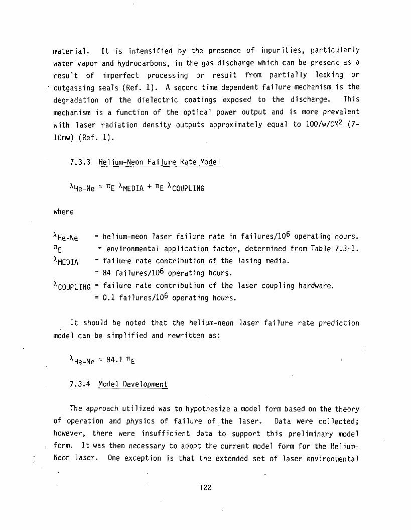
material. It is intensified by the presence of impurities, particularly
water vapor and hydrocarbons, in the gas discharge which can be present as a
result of imperfect processing or result from partially leaking or
' outgassing seals (Ref. 1). A second time dependent failure mechanism is the
degradation of the dielectric coatings exposed to the discharge. This
mechanism is a function of the optical power output and is more prevalent
with laser radiation density outputs approximately equal to 100/w/CM2 (7-
lOmw) (Ref. 1).
7.3.3 Helium-Neon Failure Rate Model
xHe-Ne = ^E XMEDIA + ^E ^COUPLING
where
xHe-Ne = helium-neon laser failure rate in failures/10^ operating hours. 71E = environmental application factor, determined from Table 7.3-1.
^MEDIA = failure rate contribution of the lasing media.
= 84 failures/10^ operating hours.
^COUPLING = failure rate contribution of the laser coupling hardware.
= 0.1 failures /106 operating hours.
It should be noted that the helium-neon laser failure rate prediction
model can be simplified and rewritten as:
*He-Ne = 84.1 *E
7.3.4 Model Development
The approach utilized was to hypothesize a model form based on the theory
of operation and physics of failure of the laser. Data were collected;
however, there were insufficient data to support this preliminary model
, form. It was then necessary to adopt the current model form for the Helium-
Neon laser. One exception is that the extended set of laser environmental
122
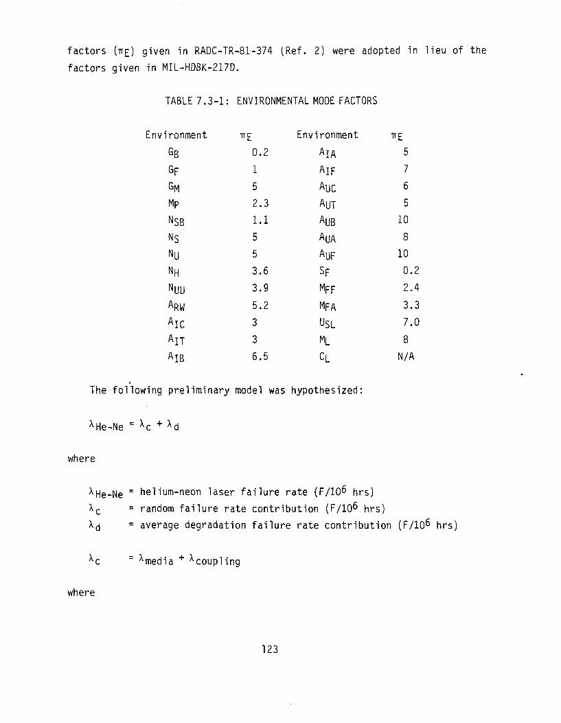
factors (TIE) given in RADC-TR-81-374 (Ref. 2) were adopted in lieu of the
factors given in MIL-HDBK-217D.
TABLE 7.3-1: ENVIRONMENTAL MODE FACTORS
Environment
GB
GF
GM Mp
NSB
Ns Nu NH NUU ARW
AlC AIT
AlB
TTE
0.2
1
5 2.3
1.1
5
5 3.6
3.9
5.2
3
3
6.5
Environment
AlA
AlF
AUC AUT
AUB
AUA
AUF
SF MFF MFA
USL ML
CL
TTE
5 7
6
5
10
8
10 0.2
2.4
3.3
7.0
8 N/A
The following preliminary model was hypothesized:
xHe-Ne = xc + xd
where
xHe-Ne = helium-neon laser failure rate (F/106 hrs)
X c = random failure rate contribution (F/10^ hrs)
X,j = average degradation failure rate contribution (F/10^ hrs)
xc = xmedia + ^coupling
where
123
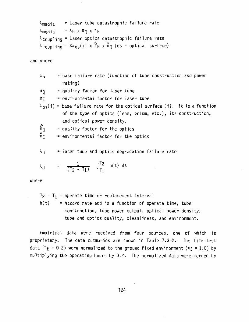
^media = Laser tube catastrophic failure rate xmedia = x b * Q x frE ^coupling = Laser optics catastrophic failure rate
Coupling = sxos(1) x ^E * TTQ (OS = optical surface)
and where
^b = base failure rate (function of tube construction and power
rating)
TTQ = quality factor for laser tube
TTE = environmental factor for laser tube
^os(i) = base failure rate for the optical surface (i). It is a function
of the type of optics (lens, prism, etc.), its construction,
and optical power density.
TTQ = quality factor for the optics A
iTE = environmental factor for the optics
^d = laser tube and optics degradation failure rate
xd = i j 1 2 h(t) dt a (T2 - Ti) JJi
where
T2 - Tj_ = operate time or replacement interval
h(t) = hazard rate and is a function of operate time, tube
construction, tube power output, optical power density,
tube and optics quality, cleanliness, and environment.
Empirical data were received from four sources, one of which is
proprietary. The data summaries are shown in Table 7.3-2. The life test
data (TE = °«2) were normalized to the ground fixed environment (TTE = 1.0) by
multiplying the operating hours by 0.2. The normalized data were merged by
124

" O C U <D TO O • « - O QJ . ,_ > .,_
o : 4-> o i > f d - o QJ
QJ t - " O • O QJ >>**»-o o . c c n
O O rd >
< i _ >-, S- I— rO CO O
CO Q 4 - • ^ t n
TD t n -—- i_ -— S- X x : QJ J Z <
3 1 SL O
• i n S_
X
m ^ - o o -o r-c cn o. -ro > o t—i
z c < i— , - H
o CO
CNJ
QJ " O
o 3
r -
ro 4-> r o
-o 4-> t n QJ 4->
QJ 4 -• r -_ J
C X QJ O
x : O 2 <—<
- I QJ O s _ > — 3 QJ
r— JD
•»— r o in 4 - Q .
O 4 - S-
o -o t n 4-> C 3 O Q .
• » - 4-> 4-> 3
X o
• • - o c o
TD
T
u ro
LiJ
f d 4-> ra
-a 4-> t n <D - M
QJ 4 -
-(— _ J
t n S_ 3 o
x :
O o o CNJ CNJ
i _ o
4 -
C 3 i _
c QJ
E 3
s_ 4-J t n C
C
o ro
4-J ro
- o
• o
QJ • t—
u _
• - M C C1J
E Q .
Z1
cr QJ
s- o ZC c n
<X> t£> t—i <£»
L D r o r— . - H I — CNJ c o r-- CNj o U"> <X> «d" CTi I—
r -< QJ OO
4-J U J i-O
a t—
CNJ i n «a- c o
KB «—I «d" CNJ
«3- «3- r-- r o c o
O r o CNJ c o ^ H
.—I r--» CNJ t£> CO i& o «—• r-«. i—i
=3 > *
-— o i i CNJ i cr»
.— re 4-> O
r -
QJ - M rC S_
o o CNJ <y> o
CO CNJ «a- O O < - CO UD O O CTi <x> CO «3" O cr* ro ro ro o r H h - U D r o «—i
«—I CNJ , -H
o o o o o O O LO O O CNJ r o «—i CNJ i n
-— o • r - CO
O CNJ O f n ^
O *3 " «—I LT) «3"
«3" O <3- CO
r o o O o
O «-H CNJ CNJ
o o «—• O «—i
O O «—• O ^ H
^ H «—I <d" ^ H ^ H
O C3 C3 O O
O O O O O
CNJ ro i n O O
• r -
s_ CD 4->
s_ o QJ
s_ Z1
• (— m 4 -
X + J
5
m + J ro
-o
-o QJ
u _
, t ^ H
<1J>« i - O . =J CO c n
*>- c . 4 _ O —
CD « " 0 >
QJ CU E +•> — o m S- — QJ
M - =J U
o c " O — CD CD ro " O
- M O •<-m 4 -
-— v> c : O CD O Q . - M U m m i _ i _ t_
- M CD X CD Q . CD i _ Q .
3 Z)
m •— - M • < - > ? ro m O
O l L i D
„ _. t ^ _ ^
CNJ r o *a -
I— o
125

source (Table 7.3-3). A homogeneity test for merging data from diverse
sources (described in Section 3.1) was applied to the environmental
normalized data. This test was applied because of uncertainty in the
operating hour estimates for the source 1 data. The results indicate that
the four data entries do not merge. Additionally the test indicated that the
source 1 data was divergent from the other data entries. The homogeneity
test was run a second time with the source 2,3 and 4 data. The second test
indicated that these three data entries can be successfully merged. Results
of the two homogeneity tests are presented in Table 7.3-4. As described in
Section 3.1, the data entries can be successfully merged if the Kolmogrov-
Smirnov (K-S) statistic is less than the K-S critical value. The 5%
significance level was chosen for this test.
TABLE 7.3-3: NORMALIZED-MERGED DATA
Source No.* Operate Hours Failure Rate (F/IO^ hours) Failed L10%CL PT EST U90%CL
1 9 4092000 1.3 2.2 3.5 2 5/10 98179 24.8/63.3 50.9/101.8 94.5/156.9
. 3 1/4 22000 4.8/79.3 45.4/181.8 176.7/363.4 4 2 15350 34.6 130.3 346.6
TOTAL 17/25 4227529 2.8/4.4 4.0/5.9 5.6/7.7
* Devices that failed to meet 80% of output power/devices that failed to meet 100% of output power
Test No.
1 2
No. of Data Entries
4 3
TABLE 7.3-4:
K-S Statistic
0.690 0.110
HOMOGENEITY TEST
K-S Critical Value
0.680 0.785
Results
can not be merged can be merged
The data from sources 2,3 and 4 were merged by the rated power of the
tube (Table 7.3-5). The data were graphed (Figure 7.3-2). The graph
suggested that the failure rate of the tube may be of the form:
Xb = A PB
126

A regression analysis (described in Section 3.1) was run on the source 2, 3
and 4 failure experience data. The <_ 80% of rated power failure criteria was
chosen since the literature (Ref. 1) indicated that most laser equipment
designs have a built-in safety margin which will allow them to operate
successfully as long as the output of the tube is greater than 80% of rated.
The results of the regression are:
Xb = 54.8 P°- 3 2
R = 0.936 = correlation coefficient
where
Xh = Ground fixed failure rate (F/106 hours)
P = rated tube power in milliwatts (mw)
The results of the regression are graphed in Figure 7.3-2. Although the
regression indicated that the tube failure rate is a function of the tube
rated power, it was felt that the data used to derive the equation were too
sparse to include in the proposed failure rate equation.
TABLE 7.3-5: DATA MERGED BY TUBE RATED POWER
Rated Power (mw)
0.5 1.0 2.0 5.0 50.0
Sample Size
5 20 33 4 1
No. Failed
1 2 3 1 1
Operate Hours
22000 34736 59653 8150 5500
Failure L10%CL
4.8 15.3 18.4 12.9 19.2
Rate (F/: PT EST
45.4 57.6 50.3 122.7 181.8
10° hou U90%C
176.8 153.2 112.0 477.3 707.3
The normalized data from Table 7.3-6 sources 2, 3 and 4 were merged to
derive a revised estimate for the Xmedia estimate currently in MIL-HDBK-217.
Since the current MIL-HDBK-217 xmedia estimate of 84F/106 hours lies within
the 80% confidence interval of the data collected from sources 2, 3 and 4,
there is no reason to reject the current estimate. Therefore it is proposed
127
that the current MIL-HDBK-217 estimate for Xmedia be retained. The data
listed in Table 7.3-2 were graphed vs the predicted failure rate (Figure 7.3-
3). The 80% confidence interval or the upper 60% confidence limit are also
shown on the graph. As can be seen by the graph the predicted value lies
within the confidence bounds of 9 of the 11 data entries, and it lies above
the other two data entries (prediction is pessimistic).
TABLE 7.3-6: REVISED A m e d i a ESTIMATE
Sample No. Operate Failure Rate (F/106 hours) Size Failed Hours L10%CL PT EST U90%CL
69 8 135529 34.3 59.0 95.9
No optics failures were reported from the four data sources; hence no
data were available to derive a revised estimate for the current MIL-HDBK-217
estimate for coupling- Therefore it is proposed that the current MIL-HDBK-
217 prediction model and estimate of ^coupling be retained.
7.3.5 References and Bibliography
References
1. Dowley, Mark W., Reliability and Commercial Lasers, Applied Optics, Vol. 21, No. 10, May, 1982.
2. IIT Research Institute, Avionic Environmental Factors for MIL-HDBK-217, Final Technical Report, RADC-TR-81-374, January, 1982.
Bibliography
Annon., Coherent Announces Automated Manufacture of Helium Neon Lasers, Product Brochure, 1982.
Dowley, Mark W., Reliability and Commercial Lasers, Applied Optics, Vol. 21, No. 10, May, 1982.
128

4 <
F ^ - ' ^ " l
<
1
•
Xb = 54.8 P 0 .32
0 . 1 0 .2 0 .5 1 2 5 10 20
RATED POWER (mw)
FIGURE 7 . 3 - 2 : FAILURE RATE VS RATED POWER
50 100
129
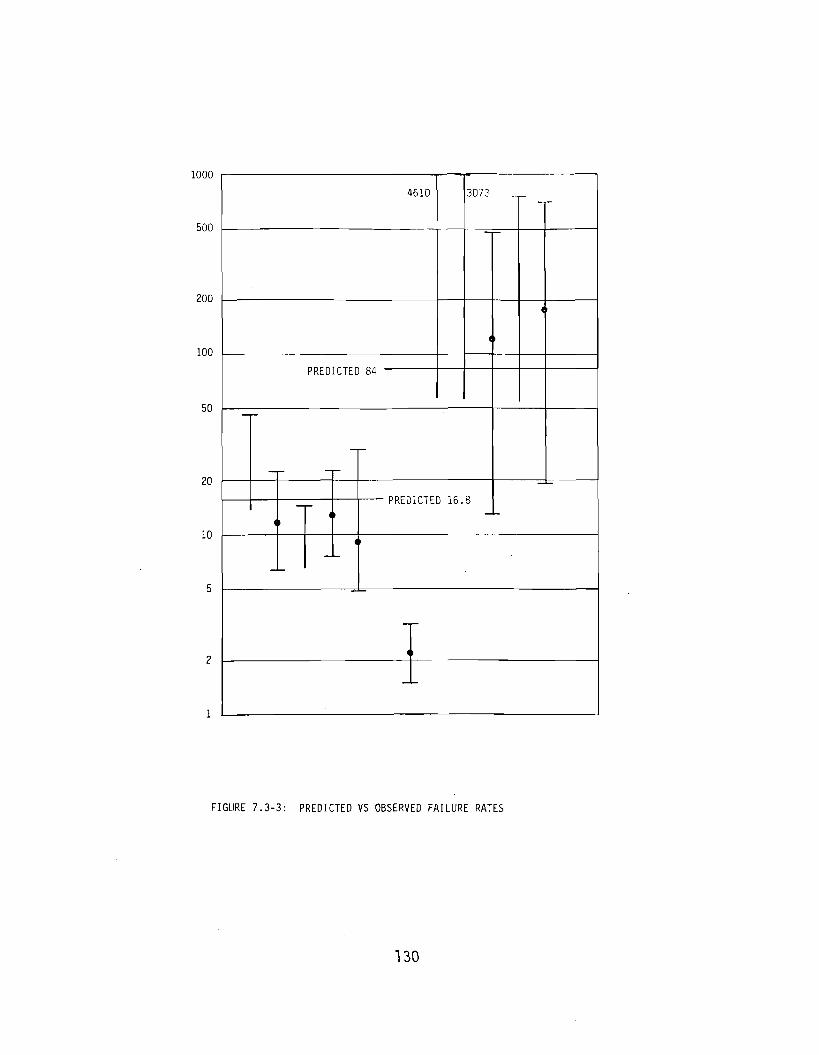
1000
500
200
100
50
20
10 < •
4610
PREDICTED
( i
i
84
3073
<
rKtulLltu lb.o
i
>
< i
<>
FIGURE 7.3-3: PREDICTED VS OBSERVED FAILURE RATES
130
Horowitz, Daniel J., Lasers (Coherent Sources), Electronic Engineers' Handbook, Second Edition, McGraw-Hill, 1982.
Martin Marietta Aerospace, Laser Reliability Prediction, Final Technical Report, RADC-TR-75-210, August, 1975.
Prather, T.W. and Ramsay, I.A., Mean Time Between Failures Data on Hughes Helium-Neon Lasers, Report No. 1, September, 1981.
7.4 Solid State, Nd:YAG Rod Laser
7.4.1 Device Construction
The Solid State Nd:YAG rod laser is a flashlamp-pumped laser that
utilizes a neodymium doped yttrium-aluminum-garnet (Nd:YAG) rod as the
lasing medium. The laser may be designed to operate in either the CW or
pulsed mode. The Nd:YAG laser is an assembly comprised of the following
subassemblies or elements:
o Nd:YAG Rod
o Flashlamp
o Optical train
o Q-Switch'
o Flashlamp power supply
o Cooling system
The design of each Nd:YAG laser may be different because the type of
flashlamp, optical train, Q-switch, power supply and cooling system may vary
from design to design. The only element that is unique is the Nd:YAG rod and
its dimensions may vary. The military users of Nd:YAG lasers include target
designators and target range finders. A detailed description of Nd:YAG
lasers and their components is given in reference 1.
131

7.4.2 Failure Modes/Mechanisms
The failure modes/mechanisms discussed below were extracted chiefly from
reference 1. The major life-limiting characteristic of Nd:YAG laser systems
is the requirement for periodic replacement of the flashlamp. The most
predominant failure mode of flashlamps is degradation sputter resulting from
a deposition mechanism which is a function of derating. Degradation of the
flashlamp can also be caused by light absorption in color centers formed by
impurities (chiefly aluminum and lithium) in the quartz tube. The type of
cooling circuit, pulse forming network and prepulsing or simmering circuit
is known to impact the life of the tube.
Greater than 90 percent of the "random" type failure mechanisms are
associated with dust on optical surfaces, misalignment or the cooling
system. Failure of the charging capacitor is known to be the predominant
problem experienced in the laser power supply.
7.4.3 Solid State, Nd:YAG Rod Laser Failure Rate Model
This section presents the failure rate prediction model for Nd:YAG
lasers. The model is:
xNd:YAG = *E ^MEDIA + XPUMP + *E *C *0S ^COUPLING
where
^Nd:YAG = the solid state neodymium doped yttrium-aluminum-garnet rod
laser failure rate in failures/106 operating hours.
TT£ = the environmental application factor, and its value is
determined from Table 7.4-1.
tylEDIA = the failure rate contribution of the lasing media, and its
value is 0.1 failures/106 operating hours for Nd:YAG lasers.
132
XPUMP = the failure rate contribution of the pumping mechanism which,
for solid state lasers, is highly affected by the flashlamp or
flash tube contribution and can be expressed as:
XPUMP = ^E x XpUMp HOURS
where
TT£ = the environmental application factor, and its value is
determined from Table 7.4-1.
XPUMP HOURS = the failure rate contribution of the flashlamp or flashtube
in failures/106 operating hours, and its value is
determined by converting pump pulses from failures per 106
pulses to failures/106 operating hours. The value for XPUMP HOURS is determined as indicated in Figures 7.4-1 or
7.4-2 as applicable.
TTQ = the coupling cleanliness factor, and its value is to be
determined from Table 7.4-2.
TTQS = the number of active optical surfaces and is determined
from Figure 7.4-3.
^COUPLING = the failure rate contribution of the laser coupling
hardware; that is, lenses, mirrors, prisms, exit window,
etc. Its value is 16.3 failures/106 operating hours for
solid state Nd:YAG lasers.
It should be noted that the solid state Nd:YAG laser failure rate
prediction model can be rewritten as:
xNd:YAG = ^E (0-1 + XPUMP HOURS + 16-3 ^C ^OS)
133

TABLE 7.4-1: SSR ENVIRONMENTAL FACTORS
Environment
GB
GF
GM
Mp
NSB NS Nu NH NUU
ARW
AlC
AIT
AlB
*E 0.2 i
5
2.3
1.1 5 5
3.6
3.9 5.2 4
3
6.5
Environment
AlA
AlF
AUC
AUT
AUB
AUA
AUF
SF MFF
MFA USL ML
CL
TTE
5
7
6
5
10 8
10
0.2 2.4
3.3 7
8
N/A
TABLE 7.4-2: COUPLING CLEANLINESS FACTORS
CLEANLINESS LEVEL (1) TTC
Rigorous cleanliness procedures, equipment, and 1 trained maintenance personnel. Plus bellows provided over optical train.
Minimal precautions during opening, maintenance, 30 repair, and testing. Plus bellows provided over optical train.
Minimal precautions during opening, maintenance, 60 repair, and testing. No bellows provided over optical train.
Notes: (1) Although sealed systems tend to be reliable once compatible materials have been selected and proven, extreme care must still be taken to prevent the entrance of particulates during manufacturing, field flashlamp replacement, or routine maintenance/repair. Contamination is the major cause of solid state laser malfunction, and special provisions and vigilance must continually be provided to maintain the cleanliness level required. T\Q values can vary from 1 up to 60.
134
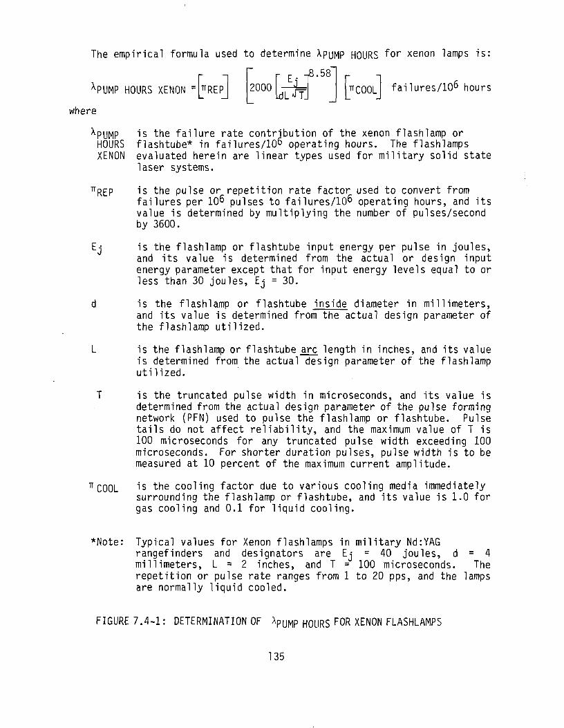
The empirical formula used to determine Xpy^P HOURS for xenon lamps is:
-,8.58" 2000 TUMP HOURS XENON =
where
^REP •JL LdL rn ^COOL failures/10^ hours
^PUMP is ^ne failure rate contribution of the xenon flash lamp or HOURS flashtube* in failures/10^ operating hours. The flashlamps XENON evaluated herein are linear types used for military solid state
laser systems.
^REP is the pulse or repetition rate factor used to convert from failures per 10& pulses to failures/10^ operating hours, and its value is determined by multiplying the number of pulses/second by 3600.
Ej is the flashlamp or flashtube input energy per pulse in joules, and its value is determined from the actual or design input energy parameter except that for input energy levels equal to or less than 30 joules, Ej = 30.
d is the flashlamp or flashtube inside diameter in millimeters, and its value is determined from the actual design parameter of the flashlamp utilized.
L is the flashlamp or flashtube arc length in inches, and its value is determined from the actual design parameter of the flashlamp utilized.
COOL
is the truncated pulse width in microseconds, and its value is determined from the actual design parameter of the pulse forming network (PFN) used to pulse the flashlamp or flashtube. Pulse tails do not affect reliability, and the maximum value of T is 100 microseconds for any truncated pulse width exceeding 100 microseconds. For shorter duration pulses, pulse width is to be measured at 10 percent of the maximum current amplitude.
is the cooling factor due to various cooling media immediately surrounding the flashlamp or flashtube, and its value is 1.0 for gas cooling and 0.1 for liquid cooling.
*Note: Typical values for Xenon flashlamps in military Nd:YAG rangefinders and designators are Ej = 40 joules, d = 4 millimeters, L = 2 inches, and T = 100 microseconds. The repetition or pulse rate ranges from 1 to 20 pps, and the lamps are normally liquid cooled.
FIGURE 7.4-1: DETERMINATION OF ApUMP H0(JRS FOR XENON FLASHLAMPS
135

The empirical formula used to determine Xp^p HOURS f° r Krypton lamp is:
XPUMP HOURS KRYPTON = 625
where
10(0.9 f) " COOL failures/106 hours
^PUMP is tne failure rate contribution of the krypton flashlamp or HOURS flashtube in failures/106 operating hours. The flashlamps KRYPTON evaluated herin are the continuous wave (CW) type and are most
widely used for commercial solid state applications. They are approximately 7mm in diameter and 5 to 6 inches long. Average power is typically 4 KW.
P is the average input power in kilowatts, and its value is determined from the actual design parameter for the flashlamp utilized.
L is the flashlamp or flashtube arc length in inches, and its value is determined from the actual design parameter of the flashlamp utilized.
^COOL 1S the cooling factor due to various cooling media immediately surrounding the flashlamp or flashtube, and its value is 1.0 for gas cooling and 0.1 for liquid cooling.
FIGURE 7.4-2: DETERMINATION OF XpUMp H0URS FOR KRYPTON FLASHLAMPS
136
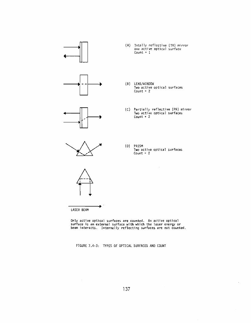
*
«
Totally reflective (TR) mirror one active optical surface Count = 1
(B) LENS/WINDOW Two active optical surfaces Count = 2
(C) Partially reflective (PR) mirror Two active optical surfaces Count = 2
(D) PRISM Two act ive opt ica l surfaces Count = 2
LASER BEAM
Only active optical surfaces are counted. An active optical surface is an external surface with which the laser energy or beam interacts. Internally reflecting surfaces are not counted.
FIGURE 7.4-3: TYPES OF OPTICAL SURFACES AND COUNT
137
7.4.4 Model Development
The model development approach used was to assume that the current model
form in MIL-HDBK-217D was correct, and to use the limited amount of field
experience data that was available to verify or disprove the model
parameters. If the data indicated that the current parameters were
incorrect, then it was planned to revise them to reflect the results of the
analysis of the data. The failure experience data collected in support of
this study are presented in Table 7.4-3. It should be noted that the source
1 through 4 data were obtained from the U.S. Air Force Maintenance Data
System and that the data are part replacements. The observed replacements
then should present an upper bound on the true number of failures incurred.
Technical information collected to allow for the calculation of a predicted
failure rate is presented in Table 7.4-4. A prediction was made on the
source 1 through 4 data. The prediction results were compared with the
observed failure rate (Table 7.4-5). A comparison of the predicted vs.
observed failure rate for those entries with observed failures showed the
following:
o The laser prediction was pessimistic for three of the four sources and for the group as a whole, and accurate for one of the sources,
o The rod prediction was optimistic for all four sources and for the group as a whole,
o The lamp prediction was optimistic for three sources, pessimistic for the other source and accurate for the group as a whole,
o The optics prediction was pessimistic for all four sources and for the group as a whole.
The published literature (Ref. 1, 2, 3, 4) indicated that the inclusion
of a "simmer" circuit should improve the life of the flashlamp. The data
were examined to determine if it substantiated these claims. A
multiplicative variable (A) was added to the xenon flash tube model. The
revised xenon failure rate model was set equal to the observed point estimate
failure rate equation (observed failures/operating time) to derive a
138

o o
o o
3 a. Q- E
CO O O O
O
O
o
CO o o o o
g o o
Q-O) O
ro S_ a: =3
o 0J -C O-I- E DUD <0
r~ ° ~"' o
o
< >-o
Wl - r -0) 4->
8 o
139

O O
D. O 0) —i
O LU or
to to
~F
c c *— X O e£ U ^->
U 1- -O O
(J +•» IT) *»- m . -*-» <— m Q. Z3 i—l o -o I O II
E U r o i t fl IT) •— •— S-—I <D -C <D
i . y i/i F Cr u m El l/> O »— •*-< C L l L V)
•— o 0 c U J * >> c
1 X> s -<D TO
-*-» c
4 - 4-> o i -
Ol (J
_ l U O
C\J I— E <u i—
•)W •»- O •on E
C3 <1J * X *"3 </l
» \£) 1— trt "I—1 <u ZJ •*-> J *
O C II O p j m o i—1 ^~ 't-XL.
O UJ n o
O - I — 1— <D ^
C D U - <U =3
r^ CT>+-» fc. w o r i i )
t 1- to E C r +•» m E
> .»- .— •»-< Z L L in
i -o
+J m
=3 •o o E
140

m —« o cr
m —< 1/1 1/1 H-
Gj O ^ r —«
.—< < \ J •—»
.—< m •—<
UJ
cr: 3 > _ J
«c U -
c
t/> t/> t— U X l D . •*- o •u CL —1
^ o <-> l/l »« J- O 3 «-•
02 ~H O ~~.
u-O w
C\J ^H
> l / l i - U J 01 c/> I—
C L J D C B O
~* C\J ~
J3 O. -D O O
o — «
141

normalized estimate for variable A. The source 2 and 3 data were combined
since they are the same system and both entries had zero failures. The
results are given in Table 7.4-6.
TABLE 7.4-6: SIMMER CIRCUIT ANALYSIS
Circuit Normalized Source Type Variable Results
1 No Simmer 19.6 10 X worse than source 2 & 3
2&3 Simmer 1.88
4 No Simmer 0.300 6 X better than source 2 & 3
As the data shows, the results are inconclusive; therefore, even though the
literature claims that a simmer circuit improves the life of the tube, the
data neither confirms nor denies it. The source 5 data is life test data on
tubes without a simmer circuit and the source 6 data is life test data on
tubes using a simmer circuit. These data show a 3:1 failure rate improvement
for tubes used with a simmer circuit. One of the reasons why the results are
inclusive may be due to the method of determining the total number of shots
accumulated by each data source. The number of equipment operating hours was
obtained through field inquiries while the number of shots per hour was
determined from technical information. It is not known whether the lasing
mechanism was inhibited during a portion of equipment operation. If it were
inhibited for a portion of the time then the observed failure rate calculated
for the laser would be optimistic. For instance, it is known that the lasing
mechanism of the AVQ-25 was inhibited for a portion of the operating time
during the Rel Demo test. The equipment which normally operates at 10 or 20
shots/second was run during the Rel Demo test on the average 1.85
shots/second of operate time. Since the data were inconclusive as to the
accuracy of the xenon lamp model as a whole, it is proposed that the current
prediction model be retained until more field experience data become
available.
142

From discussions held with optics experts, it has been determined that
optical power density is a factor that should be included in the optics
portion of the model; however, no data were obtained that could be used to
develop this hypothesis. The comparison between the predicted and observed
failure rates indicated that the optics model may be overly pessimistic, and
that the rod model may be overly optimistic. The data from sources 1 & 2
would indicate that the rod model may be optimistic (predicts a lower failure
rate) by over two orders of magnitude, and that the optics model may be
pessimistic (predicts a higher failure rate) by a factor of three. Since all
of the available data are from the same environment (A u c), it could not be
determined if the base failure rates ( rnedia anc' ^coupling) are ^n error,
and/or if it is the environmental factor (fr ) that is an error.
Since there was not sufficient data to revise the current model, it is
proposed that it be retained until data becomes available.
7.5 References and Bibliography
References
1. Martin Marietta Corporation, Laser Reliability Prediction, Final Technical Report, RADC-TR-75-210, August, 1975.
2. ILC Technology, Liquid Cooled Flashlamp Catalog.
3. IBID., Air Cooled Linear Flashlamp Catalog.
4. IBID., Internal Report, 1982.
Bibl ioqraph.y
EG&G Electro-optics Product Catalog.
ILC Technology, Liquid Cooled Flashlamp Catalog.
IBID., Air Cooled Linear Flashlamp Catalog.
Martin Marietta Corporation, Laser Reliability Prediction, Final Technical Report, RADC-TR-75-210, August, 1975.
143

Paget, Fred W., Xenon Flash tube Power Supplies, Journal of the Society of Illuminating Engineers, Vol. 4, October, 1974, pp. 223-228.
Pettifer, R.E., et.al., A Reliable 60KV Flashlamp Triggering System, Journal of Physics E, Scientific Instruments, Vol. 8, 1975.
Rehmet, M., Xenon Lamps, IEE Proceedings, Vol. 127, PT.A, No. 3, April, 1980, pp. 190-195.
144

8.0 ELECTRONIC FILTERS
8.1 Device Construction
The devices considered in this section are RFI/EMI filters per MIL-F-
15733; band pass, high pass, low pass and band suppression filters per MIL-F-
18327 and similar nonstandard filters of each type.
MIL-F-15733 filters may be a packaged assembly constructed of discrete
components soldered in place on a printed circuit card, or a hybrid type of
device consisting of capacitive-inductive elements mounted in a metal can.
RFI/EMI filters allow relatively low frequencies (50 to 400Hz) to pass
unaffected while reducing the power level of higher frequencies. Sources of
RFI/EMI vary from natural phenomenom such as lightning and cosmic noise to
man induced interference from radio transmitters and florescent lights.
These devices are not only useful in protecting electronic equipments from
unwanted RFI/EMI signals, but they can be used to protect the environment
from RFI/EMI signals generated within an equipment.
Several different internal circuit configurations are available for
RFI/EMI filters. Figure 8.1-1 presents the most popular inductor-capacitor
(LC) circuit configurations. Figure 8.1-2 presents the construction of a
ceramic-ferrite RFI/EMI filter. Reference 1 discusses the relative merits
of each circuit configuration. Filters used on AC power lines generally use
toroidal wound inductors and wound paper or paper-plastic capacitors.
Ceramic filters are widely used for low voltage applications because of their
small size. These devices also use toroidal inductors but the use of
monolithic ceramic, discoidal capacitors results in a significant reduction
in overall volume as compared to filters using paper or plastic dielectrics.
Another type of ceramic filter used for RFI/EMI suppression uses a ferrite
bead (Figure 8.1-2) as the inductive element. Here the ferrite bead
functions not as a true inductor, but as an absorber of RF energy.
145

_pr>nrr> r\ x (a) L - f i l t e r
_ r *^ rwv
;
(b) TT - f i l t e r
, L J (c) T - f i l t e r
FIGURE 8.1-1: TYPICAL LC LOW PASS FILTER CIRCUITS
FERRITE BUSHING
CLIP
TURRET OPTIONAL
SOLDER
CERAMIC
FIGURE 8.1-2: TYPICAL CERAMIC-FERRITE RFI FILTER
146
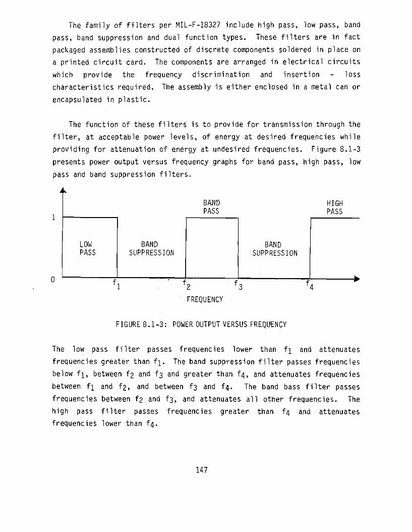
The family of filters per MIL-F-18327 include high pass, low pass, band
pass, band suppression and dual function types. These filters are in fact
packaged assemblies constructed of discrete components soldered in place on
a printed circuit card. The components are arranged in electrical circuits
which provide the frequency discrimination and insertion - loss
characteristics required. The assembly is either enclosed in a metal can or
encapsulated in plastic.
The function of these filters is to provide for transmission through the
filter, at acceptable power levels, of energy at desired frequencies while
providing for attenuation of energy at undesired frequencies. Figure 8.1-3
presents power output versus frequency graphs for band pass, high pass, low
pass and band suppression filters.
HIGH PASS
JL
LOW PASS
BAND SUPPRESSION
BAND PASS
BAND SUPPRESSION
'1 '2 '3
FREQUENCY
FIGURE 8.1-3: POWER OUTPUT VERSUS FREQUENCY
The low pass filter passes frequencies lower than f\ and attenuates
frequencies greater than f\. The band suppression filter passes frequencies
below f]_, between f2 and f3 and greater than f4, and attenuates frequencies
between fi and f2, and between f3 and fq. The band bass filter passes
frequencies between f2 and f3, and attenuates all other frequencies. The
high pass filter passes frequencies greater than fq and attenuates
frequencies lower than f4.
147
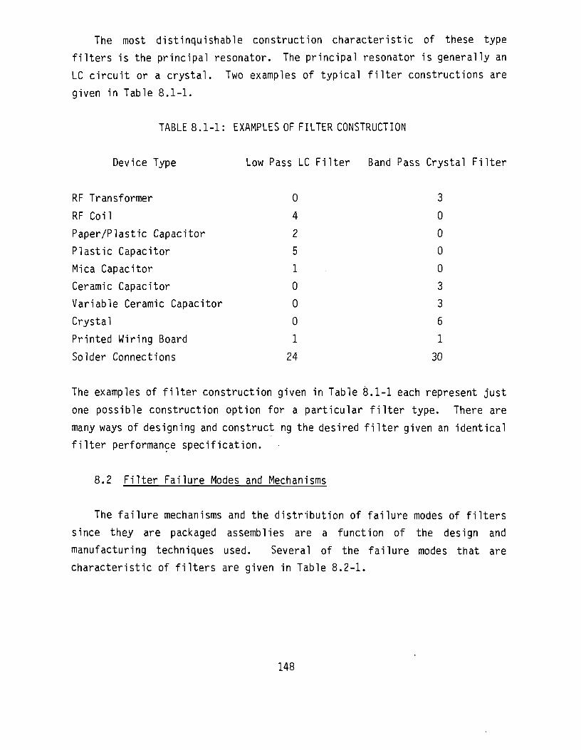
The most distinguishable construction characteristic of these type
filters is the principal resonator. The principal resonator is generally an
LC circuit or a crystal. Two examples of typical filter constructions are
given in Table 8.1-1.
TABLE 8.1-1: EXAMPLES OF FILTER CONSTRUCTION
Device Type Low Pass LC Filter Band Pass Crystal Filter
RF Transformer
RF Coil
Paper/Plastic Capacitor
Plastic Capacitor
Mica Capacitor
Ceramic Capacitor
Variable Ceramic Capacitor
Crystal
Printed Wiring Board
Solder Connections
0 4
2
5
1
0
0
0
1
24
3 0
0
0
0
3
3
6
1
30
The examples of filter construction given in Table 8.1-1 each represent just
one possible construction option for a particular filter type. There are
many ways of designing and construct ng the desired filter given an identical
filter performance specification.
8.2 Filter Failure Modes and Mechanisms
The failure mechanisms and the distribution of failure modes of filters
since they are packaged assemblies are a function of the design and
manufacturing techniques used. Several of the failure modes that are
characteristic of filters are given in Table 8.2-1.
148
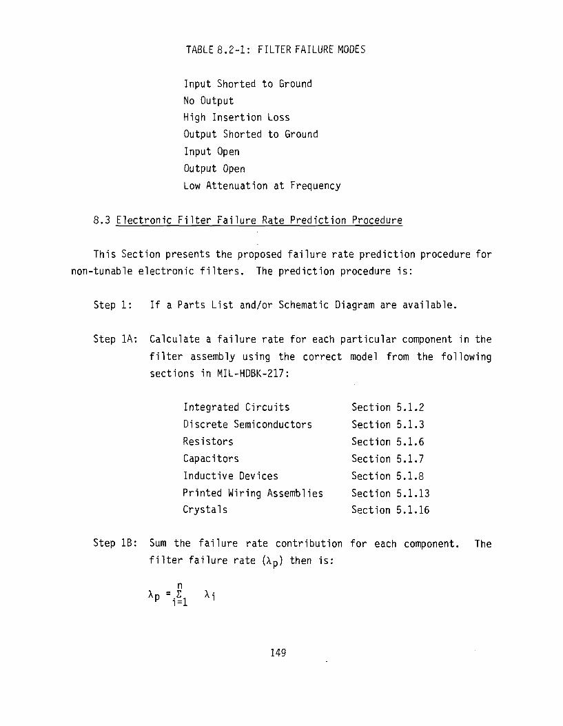
TABLE 8.2-1: FILTER FAILURE MODES
Input Shorted to Ground
No Output
High Insertion Loss
Output Shorted to Ground
Input Open
Output Open
Low Attenuation at Frequency
8.3 Electronic Filter Failure Rate Prediction Procedure
This Section presents the proposed failure rate prediction procedure for
non-tunable electronic filters. The prediction procedure is:
Step 1: If a Parts List and/or Schematic Diagram are available.
Step 1A: Calculate a failure rate for each particular component in the
filter assembly using the correct model from the following
sections in MIL-HDBK-217:
Integrated Circuits Section 5.1.2
Discrete Semiconductors Section 5.1.3
Resistors Section 5.1.6
Capacitors Section 5.1.7
Inductive Devices Section 5.1.8
Printed Wiring Assemblies Section 5.1.13
Crystals Section 5.1.16
Step IB: Sum the failure rate contribution for each component. The
filter failure rate (Xp) then is:
n
149
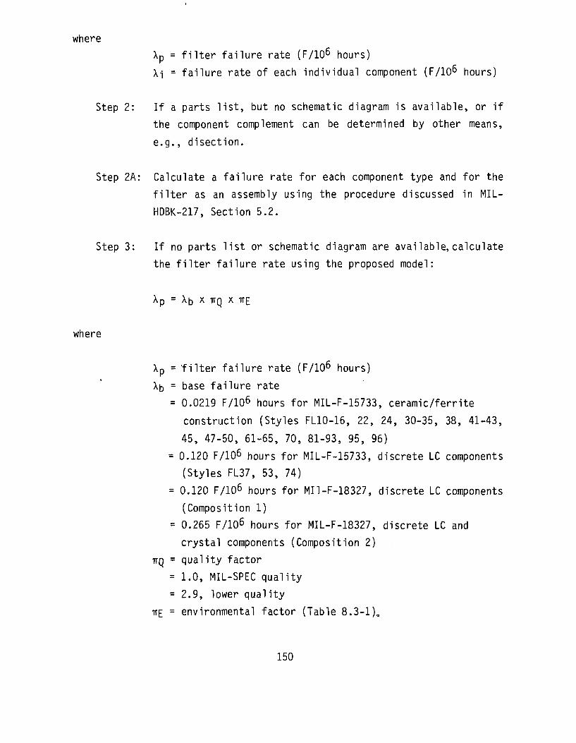
where
Xp = filter failure rate (F/106 hours)
Xi = failure rate of each individual component (F/106 hours)
Step 2: If a parts list, but no schematic diagram is available, or if
the component complement can be determined by other means,
e.g., disection.
Step 2A: Calculate a failure rate for each component type and for the
filter as an assembly using the procedure discussed in MIL-
HDBK-217, Section 5.2.
Step 3: If no parts list or schematic diagram are available, calculate
the filter failure rate using the proposed model:
X p = X b X TTQ X TTE
where
Xp = filter failure rate (F/106 hours)
X5 = base failure rate
= 0.0219 F/106 hours for MIL-F-15733, ceramic/ferrite
construction (Styles FL10-16, 22, 24, 30-35, 38, 41-43,
45, 47-50, 61-65, 70, 81-93, 95, 96)
= 0.120 F/106 hours for MIL-F-15733, discrete LC components
(Styles FL37, 53, 74)
= 0.120 F/106 hours for MI1-F-18327, discrete LC components
(Composition 1)
= 0.265 F/106 hours for MIL-F-18327, discrete LC and
crystal components (Composition 2)
TTQ = quality factor
= 1.0, MIL-SPEC quality
= 2.9, lower quality
iiE = environmental factor (Table 8.3-1),,
150

TABLE 8.3-1: ENVIRONMENTAL FACTORS
Environment
GB GF
GM Mp
NSB Ns Nu NH NUU ARW
AlC AIT
AlB
7TE
1
2.1
6 6.4
3.7
4.3 7.9 8.7
9.2
11 5.5 8.8
5.5
Environment
AlA
AlF
AUC AUT
AUB AUA
AUF SF
MFF MFA
USL ML
CL
7TE
8.8
8.8
10
13
10
13
13
1.7
6.4
8.2
14
16
120
8.4 Failure Rate Model Development
The approach utilized for model development was to treat the filter as a
packaged assembly. The rationale for this approach is based on the following
facts:
o the filter is a packaged assembly comprised of discrete components.
o every filter is functionally a frequency suppression circuit; however, the circuit design and consequently the quantity, quality and type of components used in the design varies between manufacturers.
o The filter MIL-SPEC is a functional specification and does not specify or limit internal construction.
However, it was recognized that it may not be possible for the reliability
analyst to obtain the parts list and/or schematic diagram for a filter;
therefore a default prediction procedure was necessary.
151

The approach used for development of a default filter failure rate
prediction model was to identify and quantify model parameters by analysis of
field experience data. The filter failure rate data collected in support of
this study effort are presented in Table 8.4-1.
Application and construction variables which were considered as possible
filter failure rate model modifying parameters are presented in Table 8.4-2.
The application and construction variables were determined whenever possible
for all collected data. The selection of variables to be included in the
proposed filter failure rate prediction model was based solely on the
analysis of field experience data.
Stepwise multiple linear regression analysis as described in Section 3.1
was applied to the filter failure rate data. Data records which were
included in the regression analysis are indicated in Table 8.4-1. Other data
records included insufficient part hours to estimate a failure rate without
observed failures, or insufficient detail was obtained, or the entry was
identified as an outlier or the part was outside the scope of the study.
Construction was assumed to be discrete LC unless otherwise indicated. The
regression analysis resulted in the following filter failure rate prediction
model:
Xp = Xb x ITQ x TIE
where
Xp = predicted filter failure rate in failures/10^ hours
X5 = base failure rate
= 0.0407 F/I06 hours for ceramic-ferrite construction
= 0.105 F/106 hours for discrete LC component construction
= 0.0698 F/I06 hours for discrete LC and crystal component
construction
152
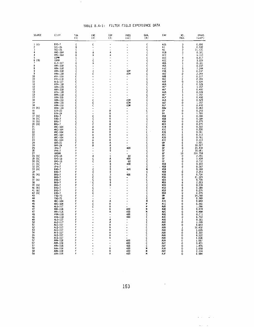
TABLE 8.4-1: FILTER FIELD EXPERIENCE DATA
SOURCE EC'JIP FUN ENC COK FREQ OUAL ENV NO. OPHRS (1 ) (2 ) ( 3 ) (H2) ( 4 ) FAIL (xlQ6)
1 2 3 t t 5 6 7 8 8 9 9
10 10 11 12 12 12 13 13 13 14 14 14 15 16 16 17 18 19 20 21 21 22 22 23 23 24 24 25 26 27 28 29
(6)
(8)
(6)
(6) (6) (6) (6)
(6) (6)
30 (6 ) 31 (6) 32 ( 6 ) 33 34
(6)
35 ( 6 ) 36 37 38 39 40 41 42 43 44 45 45 46 47 47 4B 4B 49 50 51 52 53 54 55 56 57 57 57 58 58 58
(6)
(6) (6) (6) (6)
BRD-7 SQS-26 SQS-26 ARC-164 ARC-164 COW COHM ALC-117 ARN-118 ARN-118 ARN-118 APJi-llB ARN-11B ARN-118 ALQ-117 ARN-11B ARN-118 ARN-11B ARN-118 ARN-118 ARN-118 ARN-11B ARN-11B ARN-11B ARN-11B GRR-23 GRR-24 BRD-7 8RD-7 BRD-7 BRD-7 ARC-164 ARC-164 ARC-164 ARC-164 ARC-164 ARC-164 GRR-23 GRR-24 UYK-7 UYK-7 RADAR GYQ-18 GYQ-18 GYQ-1B UYK-7 UYK-7 BRD-7 BR0-7 BRD-7 BR0-7 BRD-7 BRD-7 BR0-7 BRD-7 BRD-7 BRO-7 TSQ-73 TSQ-73 ARC-164 ARC-164 ALQ-117 ARN-118 ARN-118 ARN-118 ARN-118 ALO-117 ALO-117 ALO-117 ALO-117 ALO-117 ALO-117 ALO-117 ALQ-117 ARN-118 ARN-118 ARN-11B ARN-11B ARN-118 ARN-118
C
--A A
-C A
--C C
---------c c c ---c c c c A A A A A A B B
---A C C
--C
c c c c c c c c c . -c c c -. ----------------
---A A
--------------------B B B B B B B B B B B B A A 0 0
-c A A D D 0 D D 0 0 D D
-----A A A A A
--A A A A A A A A
---A A A
----------63M 63H
----_ ----63M 63M 63M
---------------400
--60 400
60 400
-400
_ 400
-_ _ ---------400 400 400 400
--------400 400 400 400 400 400
C C C C C C C C C C C C C C C C
c c c c c c c c c c r. c c c c c c c c c c c c c c c c c c c c M
c c c c c c c c c c c M M M H M C
c c c c c c c c c c c c H M M
NSB NS NS AIB AIC A1C AIC AUB AUB AUC AUB AUC AUB AUC AUB AUA AUT AUF AUA AUT AUF AUA AUT AUF ARW GM GM NSB NSB NSB NSB AIB AIC AIB AIC AIB AIC GH GM GF GF GF GF GF GF NSB
. NSB NSB NSB NSB NSB NSB NSB NSB NSB NSB NSB GH GM AIB AIC AUB AUB AUC AUB AUC AUB AUB AUB AUB AUB AUB AUB AUB AUA AUT AUF AUA AUT AUF
0 0 2 0 1 4 2 1 1 5 0 0 3 2 0 2 6 2 5 1 1 0 0 0 1 0 0 1 0 0 0 0 0 1 0 0 0 0 0 0 2
10 0 0 0 0 0 1 0 0 2 0 0 0 0 0 0 0 0 0 0 0 0 0 0 0 1 0 0 1 0 0 0 0 0 0 0 0 0 0
0.092 0.532
25.135 0.161 0.113 0.917 0.229 0.161 0.237 2.244 0.237 2.244 0.237 2.244 4.824 0.529 1.157 0.492 0.529 1.157 0.492 0.529 1.157 0.492 0.063 0.253 1.701 0.184 0.184 0.275 0.275 0.322 0.226 0.161 0.113 0.161 0.113 1.521
10.207 21.414 16.061
314.758 2.491 1.424 0.712 0.222 0.167 0.184 2.203 0.734
31.123 0.734 2.203 0.91B 0.184 0.275 0.275
14.760 0.369 0.643 0.551 1.286 0.474 4.488 0.711 6.732 0.161 1.126 0.643
10.432 1.026 0.322 0.322 4.824 1.5B7 3.471 1.476 1.058 2.314 0.984
153

TABLE 8.4-1: FILTER FIELD EXPERIENCE DATA (CONT'D)
SOURCE EQUIP FUN ENC COM FREQ QUAL ENV NO. OPHRS ( 1 ) ( 2 ) ( 3 ) (Hz) ( 4 ) FAIL ( * 1 0 6 )
59 (6 ) 60 ( 6 ) 6 ] (6) 62 ( 6 ) 63 ( 6 ) 64 (6 ) 65 (6 ) 66 ( 6 ) 67 (6 ) 6B (6 ) 69 (6 ) 70 (6 ) 71 ( 6 ) 72 (6 ) 73 (6 ) 74 (6 ) 75 ( 6 ) 76 ( 6 ) 77 ( 6 ) 78 ( 6 ) 79 (6 ) 8D (6 ) 81 ( 6 ) 82 ( 6 ) 83 (7 ) 84 (6 ) 85 (6 ) 86 (7 ) 87 88 (6 ) 89 (6 ) 90 (6 ) 91 (6 ) 92 ( 6 ) 93 (6 ) 94 ( 6 ) 95 ( 6 ) 96 ( 9 ) 97 ( 9 ) 98 ( 7 ) 99 (8 ) 100 101 (9 ) 102 (9 ) 103 (9 )
TOTAL
ARN-11B ARN-11B GYQ-16 BRD-7 BRD-7 BRD-7 BRD-7 BRD-7 BRD-7 BRD-7 BRD-7 BRD-7 BRD-7 BRO-7 BRD-7 BRD-7 BRD-7 ALQ-117 TSQ-73 RAOAR ARN-11B ARN-11B ARC-164 ARC-164 RAOAR RAOAR SQS-26 SQS-26 SQS-26 ARC-164 ARC-164 ARC-164 ARC-164 ARC-164 ARC-164 ARC-164 ARC-164 GRR-24 GRR-23 SENSOR BRD-7
-PWR EQUIP PWR EQUIP PWR EQUIP
F F F
-F F C C C c c c c c c c c F A B C C B B
-C c -F F C C C C F F C G G
-F F ( 5 ) F r F
--A
-A A C C C C c c c c c c c -c . c --_ _ -. -_ -_ _ ---. -_ _ -c ----
-A c ---B B B B B B B B B B B A
--_ ----_ -------------A
-----
4 DO 4 DO 60
-60
---------------63M
-------------------400
-60 60 60
C M C M C C c c c c c c c c c c c c c -c c c c c c c c c c c c c c c c c c c c c c c c c
ARW ARW GF NSB NSE NSB NSB NSB NSB NSB NSB NSB NSB NSB NSB NSB NSB AUB GM GF ARW ARW AI Al GF GF NS NS NS AI AI AI AI AI AI AI AI GM GM GF NSB GF GF GF GF
D 0 0 0 0 0 0. 0 0 0 0 0 0 0 0 0 0 0 0 0 0 0 0 0 0 0 0 0 0 0 0 0 0 0 0 0 0 4 1 0 4 1 4 2 0
73
0 . 1 2 6 0.189 0.356 0.092 0.092 0.092 0.092 0.092 0.092 0.092 0.092 0.092 0.092 0.092 0.092 0.092 0.092 0.161 0.123 0.223 0.063 0.063 0.320 0.080
28.174 0.8B9 0.532 2.015 6.839 O.OBO 0.080 0.080 0.240 0.160 0.080 0.08D 0.080 1.701 0.253 8.360 0.184 0.736 3.326 3.211 0.642
580.955
NOTES: ( 1 ) A - High Pass, B - Low P i s s , C • Band Pass, D •= Band Suppression F « RF I , G - Tunable
( 2 ) A « Metal Encased (non -hermet ic ) , B - Encapsulated (non-hermet ic) C ° Hermet ica l ly Sealed
(3 ) A = LC, B • C r y s t a l , C - Other E lec t romechanica l , D • F e r r i t e ( 4 ) C * Cownercial q u a l i t y . M = MIL-SPEC q u a l i t y (6 ) EMI F i l t e r (6) Insufficient part hours (7) Insufficient detail (8) Identified as an outlier (9) Part outside scope of study
154

TABLE 8.4-2: FILTER CONSTRUCTION AND APPLICATION VARIABLES
I. Function A. High Pass B. Low Pass C. Band Pass D. Band Suppression E. Dual Functioning F. Radio Frequency Interference G. Tunable
II. Enclosure Type A. Metal Encased (non-hermetic) B. Encapsulated (non-hermetic) C. Hermetically Sealed
III. Composition A. LC B. Crystal C. Other Electromechanical D. Ferrite E. Other
IV. Quantity of Terminals
V. Current Level A. Rated B. Actual
VI. Voltage Level A. Rated B. Actual
VII. Frequency
VIII. Temperature (°C) A. Rated
B. Actual
IX. Quality Level
X. Environment
155
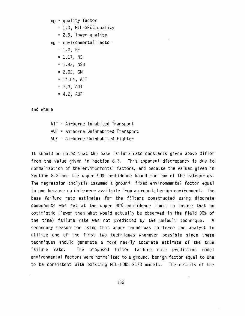
TTQ = quality factor
= 1.0, MIL-SPEC quality
= 2.9, lower quality
TT£ = environmental factor
= 1.0, GF
= 1.17, NS
= 1.83, NSB
= 2.02, GM
= 14.04, AIT
= 7.3, AUT
= 4.2, AUF
and where
AIT = Airborne Inhabited Transport
AUT = Airborne Uninhabited Transport
AUF = Airborne Uninhabited Fighter
It should be noted that the base failure rate constants given above differ
from the value given in Section 8.3. This apparent discrepancy is due to
normalization of the environmental factors, and because the values given in
Section 8.3 are the upper 90% confidence bound for two of the categories.
The regression analysis assumed a ground fixed environmental factor equal
to one because no data-were available from a ground, benign environment. The
base failure rate estimates for the filters constructed using discrete
components was set at the upper 90% confidence limit to insure that an
optimistic (lower than what would actually be observed in the field 90% of
the time) failure rate was not predicted by the default technique. A
secondary reason for using this upper bound was to force the analyst to
utilize one of the first two techniques whenever possible since these
techniques should generate a more nearly accurate estimate of the true
failure rate. The proposed filter failure rate prediction model
environmental factors were normalized to a ground, benign factor equal to one
to be consistent with existing MIL-HDBK-217D models. The details of the
156

regression analysis are given in Table 8.4-3. Base failure rate, quality
factor and environment factor were defined by the following equations:
Xb = exp(b0 + biXi + b2X2)
Xi,X2 = (0,0), RFI Filters, ferrite-ceramic .
Xi,X2 = (1.1), Discrete LC with crystal
Xi,X2 = (0,1), Discrete LC
TTQ = exp(b3X3)
X3 = 0, MIL-SPEC
X3 = 1, lower quality
TTE = exp(b4X4 + b5X5 + b6X6 + b7X7 + b8X8 + bgXg)
X4,X5,X6,X7,X8,X9 = (0,0,0,0,0,0), GF
X4,X5,X6,X7,X8,X9 = (1,0,0,0,0,0), NS
X4,X5,X6,X7,X8,Xg = (0,1,0,0,0,0), NSB
X4,X5,X6,X7,X8,X9 = (0,0,1,0,0,0), GM
X4,X5,X6,X7,X8,X9 = (0,0,0,1,0,0), AIT
X4,X5,X6,X7,X8,X9 = (0,0,0,0,1,0), AUT
X4,X5,X6,X7,X8,Xg = (0,0,0,0,0,1), AUF
The Xi variables are "dummy variables" used to quantify qualitative
factors.
TABLE 8.4-3: RESULTS OF FILTER REGRESSION ANALYSIS
Variable (Xi) C
Xl
X2
X3
X4
X5
X6
X7
X8
Xg
Constant
rficient (b-j)
0.951720
•0.411436
1.067148
0.157188
0.605001
0.702430
2.642144
1.988904
1.435398
3.201837
Standard Error
0.5764
0.9241
0.9048
1.0703
0.9994
0.9554
1.0633
0.7691
0.9850
F-Rat
2.74
0.20
1.39
0.02
0.37
0.54
6.17
6.69
2.12
157
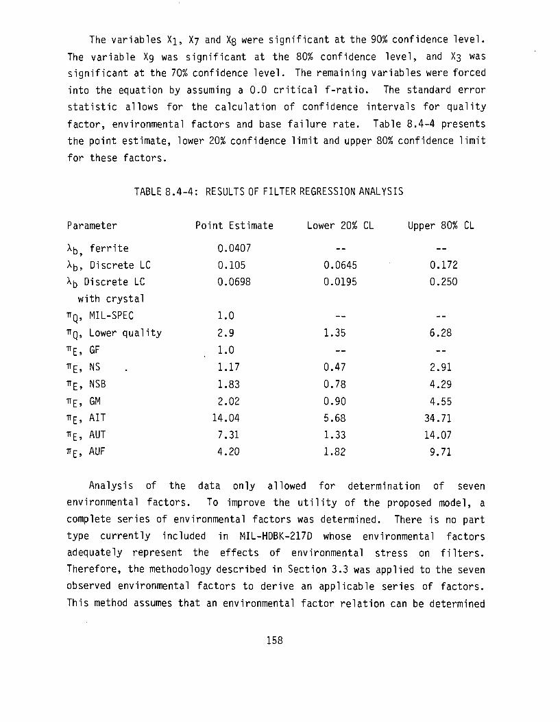
The variables Xi, X7 and Xs were significant at the 90% confidence level.
The variable Xg was significant at the 80% confidence level, and X3 was
significant at the 70% confidence level. The remaining variables were forced
into the equation by assuming a 0.0 critical f-ratio. The standard error
statistic allows for the calculation of confidence intervals for quality
factor, environmental factors and base failure rate. Table 8.4-4 presents
the point estimate, lower 20% confidence limit and upper 80% confidence limit
for these factors.
TABLE 8.4-4: RESULTS OF FILTER REGRESSION ANALYSIS
Parameter
Xj-, ferrite
X5, Discrete LC
X-b Discrete LC
with crystal
TTQ, MIL-SPEC
TTQ, Lower quality
*E, GF
*E. NS
TTE, NSB
TTE, GM
TTE, AIT
TTE, ALIT
TTE, AUF
Point Estimate
0.0407
0.105
0.0698
1.0
2.9
1.0
1.17
1.83
2.02
14.04
7.31
4.20
Lower 20% CL
—
0.0645
0.0195
—
1.35
—
0.47
0.78
0.90
5.68
1.33
1.82
Upper 80% CL
—
0.172
0.250
—
6.28
—
2.91
4.29
4.55
34.71
14.07
9.71
Analysis of the data only allowed for determination of seven
environmental factors. To improve the utility of the proposed model, a
complete series of environmental factors was determined. There is no part
type currently included in M1L-HDBK-217D whose environmental factors
adequately represent the effects of environmental stress on filters.
Therefore, the methodology described in Section 3.3 was applied to the seven
observed environmental factors to derive an applicable series of factors.
This method assumes that an environmental factor relation can be determined
158
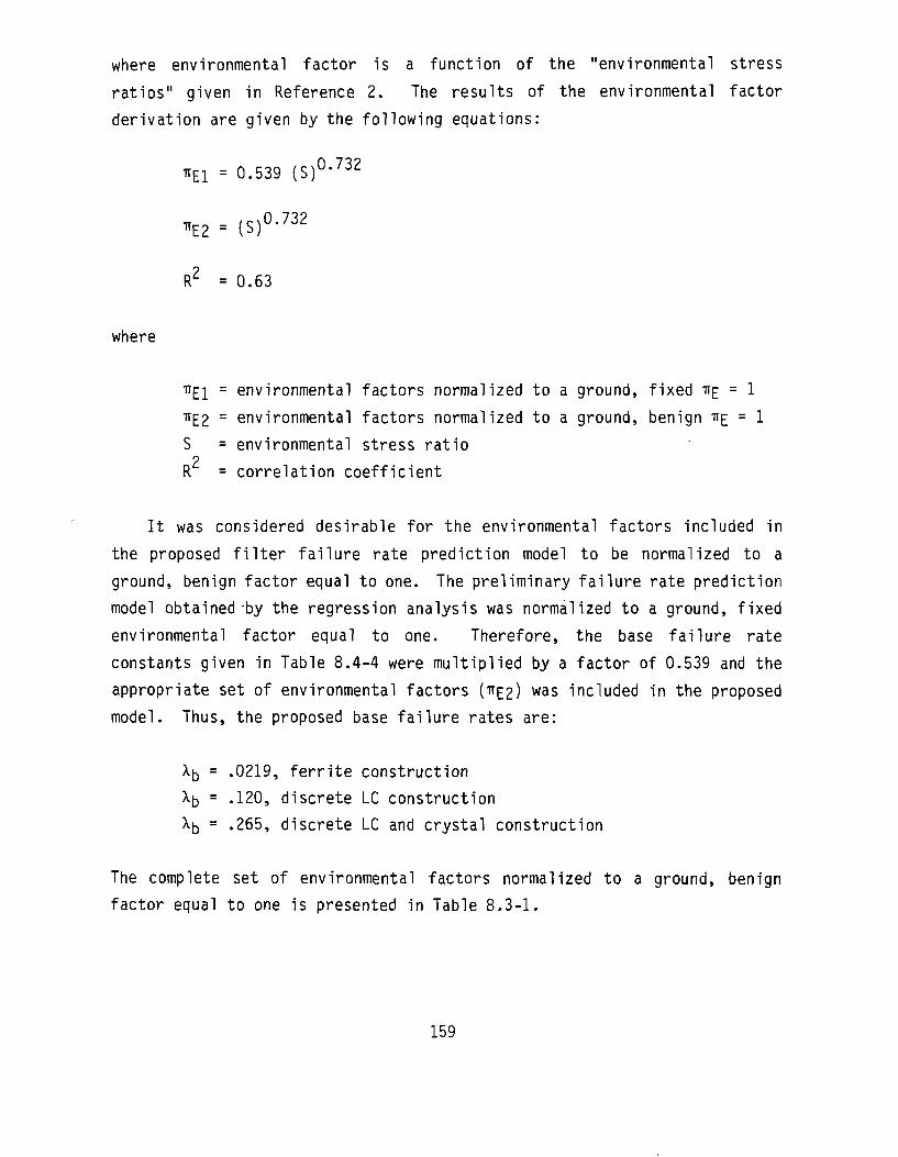
where environmental factor is a function of the "environmental stress
ratios" given in Reference 2. The results of the environmental factor
derivation are given by the following equations:
TTE1 = 0.539 ( S ) 0 ' 7 3 2
*E2 - ( S ) 0 ' 7 3 2
R2 = 0.63
where
TTQ = environmental factors normalized to a ground, fixed TT = 1
TT£2 = environmental factors normalized to a ground, benign TTE = 1
S = environmental stress ratio 2
R = correlation coefficient
It was considered desirable for the environmental factors included in
the proposed filter failure rate prediction model to be normalized to a
ground, benign factor equal to one. The preliminary failure rate prediction
model obtained by the regression analysis was normalized to a ground, fixed
environmental factor equal to one. Therefore, the base failure rate
constants given in Table 8.4-4 were multiplied by a factor of 0.539 and the
appropriate set of environmental factors (TTE2) was included in the proposed
model. Thus, the proposed base failure rates are:
X^ = .0219, ferrite construction
X5 = .120, discrete LC construction
X^ = .265, discrete LC and crystal construction
The complete set of environmental factors normalized to a ground, benign
factor equal to one is presented in Table 8.3-1.
159

Normalization of the base failure rate and the environmental factors
concluded the failure rate prediction model development for filters. The
proposed model presents failure rate as a function of construction, quality
level and application environment. The use of this proposed model will
improve the reliability prediction capabilities for equipments designed with
filters.
8.5 References and Bibliography
References
1. Jones, Edwin C. Jr., and Hale, Harry W., Filters and Attenuators, Section 12, Electronics Engineers' Handbook, Second Edition, McGraw-Hill, 1982.
2. Kremp, B.F. and E.W. Kimball, Revision of Environmental Factors for MIL-HDBK-217B, Final Technical .Report, RADC-TR-80-299, September, 1980.
Bibliography
Curtis Industries, Inc., RFI Power Line Filters, Catalog No. 481.
Electronic Products, EMI/RFI Filters, One Answer To Electrical Pollution, October, 1978, pp 35-40.
Eric Technological Products, LTD., Filter Connectors, Catalog FC-1255R.
Jones, Edwin C , Jr., and Hale, Harry W., Filters and Attenuators, Section 12, Electronics Engineers' Handbook, Second Edition, McGraw-Hill,, 1982.
Kremp, B.F. and E.W. Kimball, Revision of Environmental Factors for MIL-HDBK-217B, Final Technical Report, RADC-TR-80-299, September, 1980.
Mann, John E., Failure Analysis of Passive Devices, 16th Annual Reliability Physics Proceedings, 1978, pp 89-92.
160

9.0 SOLID STATE RELAYS
9.1 Part Description
A solid state relay (SSR) is a switching assembly (either hybrid or
discrete components) which controls load currents through the use of solid
state switches such as triacs, SCRs, or power transistors. These switching
elements are controlled by input signals coupled to the switching devices
through various isolation mechanisms such as reed relays, transformers, or
optoisolators. Snubber circuits or zero-crossing detectors which reduce
spikes and transients produced by interupting load currents are also used in
some solid state relays.
Solid state relays in general incorporate the use of a heat sink to
minimize operating temperature. These devices generate heat because of the
voltage drop which is present in semiconductor devices. For example, a 40
amp SSR will typically drop 1.2 volts during conduction and in turn dissipate
50 watts of heat. However, no special system design is required because
cooling and heat sinking methods are adequate.
9.2 Failure Modes and Mechanisms
Solid state relays are not susceptible to wear out from on/off cycling
like electromechanical relays. Failures normally occur due to faulty SCR or
triac switching. The most common failure mode is when a solid state relay
falsely turns-on. Several failure mechanisms causing this phenomenom are:
1) operating temperatures which exceed the thyristor rating.
2) transients from the switched load or from an AC line could momentarily exceed the thyristor breakover voltage.
3) steeply rising load voltages could couple into the thyristor input through strong capacitances in the thyristor. (called dv/dt turn-on)
161

To help eliminate dv/dt turn-on, the use of back to back SCRs with reverse
bias can be used in place of triacs in the solid state relay.
The main failure mechanism for solid state relays is mechanical fatigue
of the power semiconductor structure due to thermal cycling. The effects of
cycling can be controlled, however, through the matching of load cycling
characteristics to relay characteristics.
9.3 Solid State Relay (SSR) Failure Rate Prediction Procedure
This Section presents the proposed failure rate prediction procedure for
solid state relays. The prediction procedure is:
Step 1: If a Parts List and/or Schematic Diagram are available.
Step 1A: Calculate a failure rate for each particular component in the
SSR assembly using the correct model from the following
sections in MIL-HDBK-217:
Integrated Circuits Section 5.1.2
Discrete Semiconductors Section 5.1.3
Resistors Section 5.1.6
Capacitors Section 5.1.7
Inductive Devices Section 5.1.8
Relays Section 5.1.10
Printed Wiring Assemblies Section 5.1.13
Step IB: Sum the failure rate contribution for each component. The SSR
failure rate (Xp) then is:
n XP "-j=i Xi
where
162
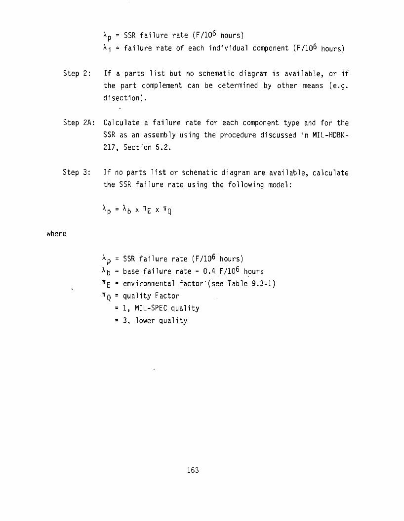
Xp = SSR failure rate (F/1C-6 hours)
X-j = failure rate of each individual component (F/106 hours)
Step 2: If a parts list but no schematic diagram is available, or if
the part complement can be determined by other means (e.g.
disection).
Step 2A: Calculate a failure rate for each component type and for the
SSR as an assembly using the procedure discussed in MIL-HDBK-
217, Section 5.2.
Step 3: If no parts list or schematic diagram are available, calculate
the SSR failure rate using the following model:
where
X p = SSR failure rate (F/106 hours)
^b = base failure rate = 0.4 F/10^ hours 77 E = environmental factor'(see Table 9.3-1) 77 Q = quality Factor
= 1, MIL-SPEC quality
= 3, lower quality
163

TABLE 9.3-1: SSR ENVIRONMENTAL FACTORS
Environment
GB GF
GM Mp
NSB Ns
Nu NH NUU ARW
AlC
AIT
AlB
TTE
1
3.3
13
10
5.2
7
17
16 17
23
6.5
9.5 24
Environment
AlA
AlF
AUC
AUT
ALIB
AUA
AUF
SF MFF
MFA
USL ML
CL
E 13
22
11
16
40
24
38
0.85
10
14
31
35 590
9.4 Failure Rate Model Development
The approach utilized for model development was to treat the SSR as a
packaged assembly. The rationale for this approach is based on the following
facts:
o the SSR is either a packaged assc.ibly comprised of discrete components, or a hybrid assembly.
o every SSR is functionally a single pole-single throw (SPST) relay; however, the circuit design and consequently the quantity, quality and type of components used in the design varies between manufacturers.
o The SSR MIL-SPEC is a functional specification and does not specify or limit internal construction.
However, it was recognized that it may not be possible for the reliability
analyst to obtain the parts list and/or schematic diagram for a SSR;
164
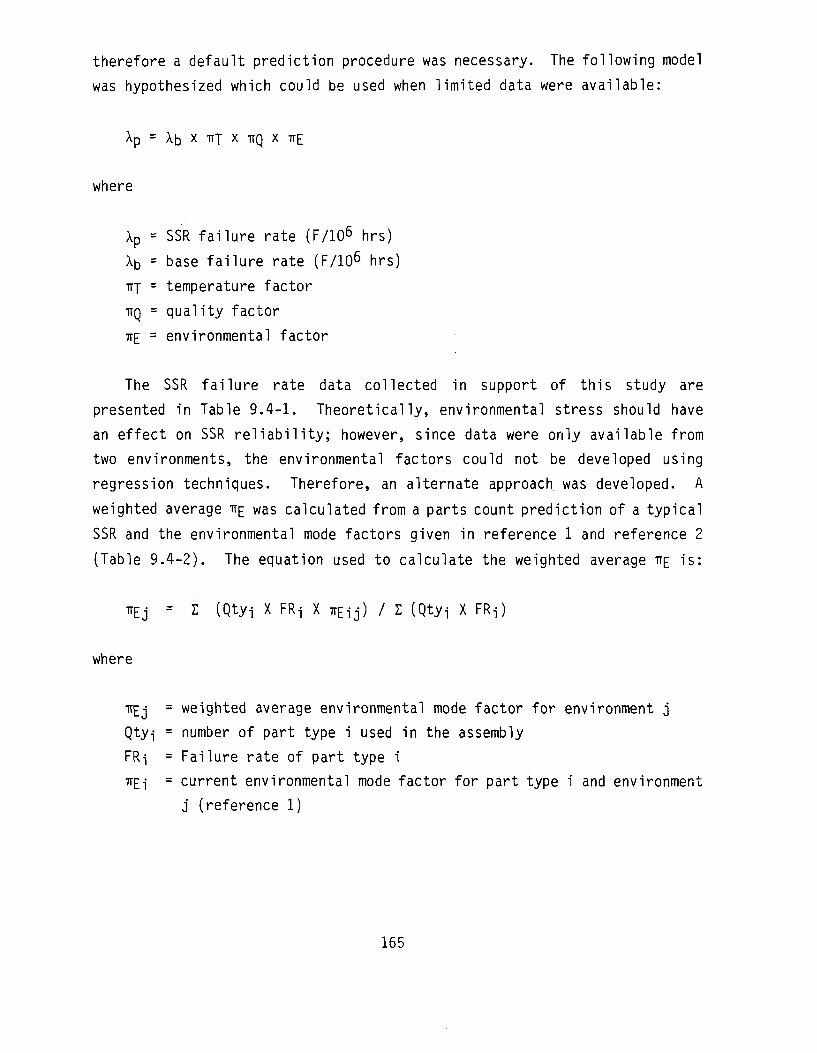
therefore a default prediction procedure was necessary. The following model
was hypothesized which could be used when limited data were available:
Xp = X b X 7TT X 7TQ X 7TE
where
Xp = SSR failure rate (F/106 hrs)
Xb = base failure rate (F/106 hrs)
TTJ = temperature factor
TTQ = quality factor
TTE = environmental factor
The SSR failure rate data collected in support of this study are
presented in Table 9.4-1. Theoretically, environmental stress should have
an effect on SSR reliability; however, since data were only available from
two environments, the environmental factors could not be developed using
regression techniques. Therefore, an alternate approach was developed. A
weighted average TIE was calculated from a parts count prediction of a typical
SSR and the environmental mode factors given in reference 1 and reference 2
(Table 9.4-2). The equation used to calculate the weighted average TTE "is:
*Ej = 2 (Qtyi X FRi X TTEij) / 2 (Qtyi X FRi)
where
TTE j = weighted average environmental mode factor for environment j
Qty-j = number of part type i used in the assembly
FRi = Failure rate of part type i
TTEi = current environmental mode factor for part type i and environment
j (reference 1)
165

o U3
o o
0>
10 l— or 1/1
0) r o un s- i— ZJ a . .-I O
10 _J Ll_ (_>
o
<D +-> *d s_ cu
,—. (/)l£) J- O 13 H O
Q.3I X o *~-
O > ^H
I <u C D .
• i - > > 3 I— c r U l
£ S- HI (O 4-»
r— in O > ,
ir> i n
166
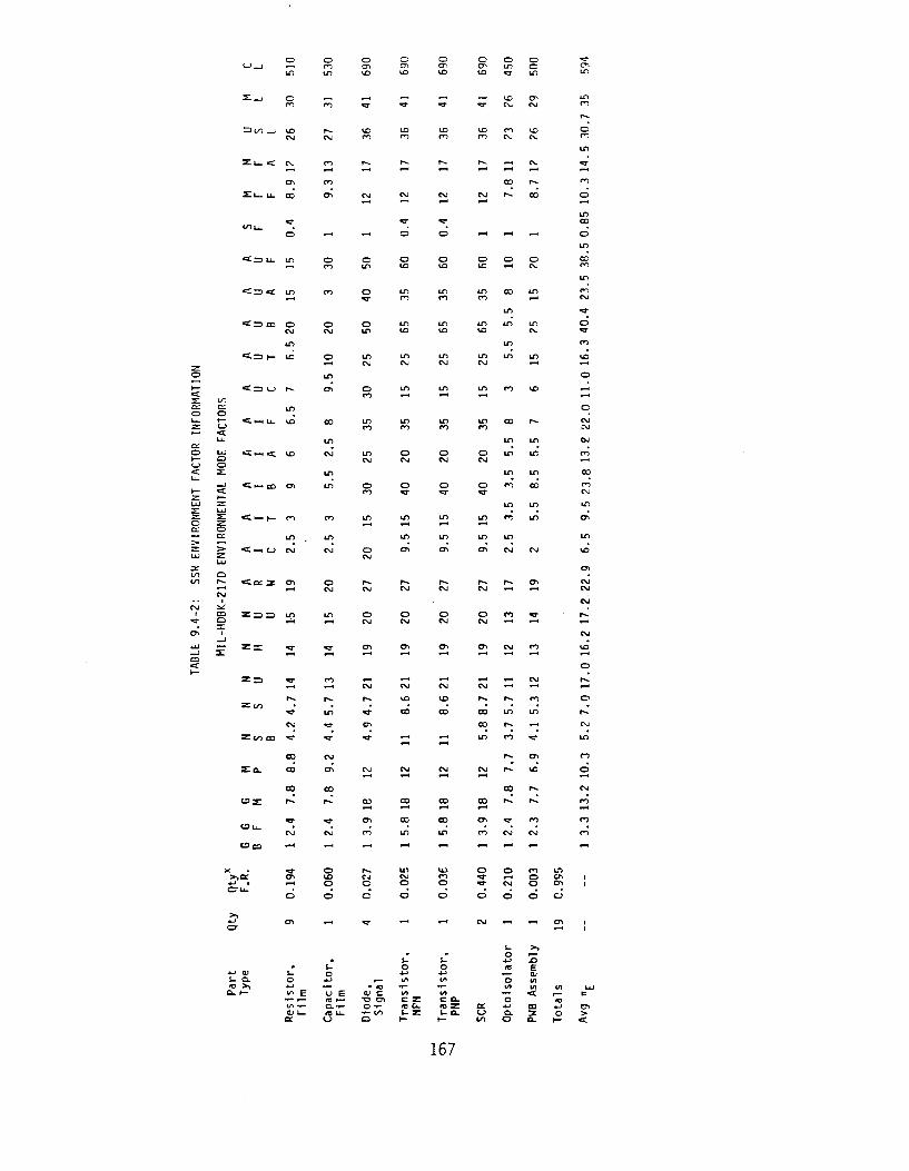
CO
CM r -
O - H ^ H rt
CO
o
< D U . ID
O CC IT) ID CO ID
• I r s to o I D I D ID
•31=3 >— vo
o
MAT
cc o ~ S "
c: o *-
IS)
cc o »— t_>
LL.
U J
« t = 3 <_J
< M l L
*3I t-H < ;
T-^
in in in
in o vo
i n
o CNJ
o
CO
i n
i n
i n
m
T-^
i n
i n
i n
CO
-•-'»— rn
< « - H O CM
in in Cft CM CM
< a » on <—I CM CM <—• ^ H
Z = 3 = > i n <—• CM
Z = ) ,—I ,—I CM
•>«. <X)
CTi C M r o
CM «-H .-H
co in m co r^ <—i
«—i *—i in
E n .
c=Z
COti.
CO t o
X >>o:
4-) • C U .
>> 4-)
cr
co CO
co r^
2.4
0.19
4
Ol
CO
CO
CM
CO
CTi
r»«.
CO r»«.
~
ic
r-* r»«.
n
^ H O C J CM
o o
d d
o o L.*) <—I © Cft CM O On
^H , - f CM <—• <—I
4-> QJ l_ CL iO >>
CL t—
i_ O 4->
m E in «i-O Li-
CC
i_
4->
u E fO p— C L - f -fU U -o
r—
QJ C
"O en O * ^
•r- (/) O
i_
o 4-> 1/)
IS) C Z ro CL. I - Z
t—
iT o
4-> l/>
IS) C fO i_
»—
C L
Z CL
or o CO
tor
o IS)
•»» o 4-> CL
o
bly
E in in
«t CO 3 CL
4->
»—
167
The factors were then rounded to two significant digits because of the
uncertainity of the data.
The failure experience data shown in Table 9.4-1 for sources 1, 2, 3, 4
and 5 were normalized to the ground benign environment (Gg) by the TTE'S
derived above. The normalized data for sources 1, 2, 3 and 4 were then
subjected to a regression analysis as described in Section 3.1 in order to
ascertain if there was a significant difference between quality levels, and,
if so, to derive a quantitative estimate of the difference. The source 5
data were deleted from the analysis because the quality level was unknown.
The sources 6 and 7 data were deleted because of the low number of operating
hours that were accumulated on the devices. The results of the regression
are shown in Table 9.4-3.
TABLE 9.4-3: SSR REGRESSION ANALYSIS RESULTS
Variable Coefficient (1) STD-Error F-Ratio
MIL-STD Quality -1.173333 (0.3) 2.2983 0.26
Commercial Quality (1.0)
Constant -0.068846 (0.933)
Notes: (1) Numbers in paranthesis are the transformed parameters
Quality was found to be significant at the 30% level. The low level of
significance was attributed to the sparsity of the data (4 data entries).
Even though the level of significance was not high (30%), it is proposed that
it be included in the prediction model since quality should be a significant
factor affecting reliability. The proposed quality factors (TTQ) are:
MIL-STD Quality 1
Commercial Quality 3
168

The factors were rounded to one significant digit because of the uncertainty
of the data.
The base failure rate factor (Xb) was derived by taking the average value
of the upper 90% confidence bounds on the source 1 through 5 and source 7
data. The upper 90% confidence bounds were calculated for data normalized to
a MIL-SPEC part in a ground, benign environment. The source 5 data were
assumed to be MIL-SPEC quality. This should be a realistic assumption since
the equipment is a missile site radar. The average of the upper 90%
confidence bounds was chosen to insure that an optimistic (lower than what
would actually be observed in the field 90% of the time) failure rate was not
predicted by the default technique. A secondary reason for using this upper
bound was to force the analyst to utilize one of the first two techniques
whenever possible since these techniques should generate a more nearly
accurate estimate of the true failure rate. The data from source 6 was
deleted from the analysis because no failures were observed and less than
1,000,000 normalized part hours were accumulated on the devices. The average
of the 90% confidence bounds is 0.392F/106 hours. Due to the uncertainty in
the method of derivation, the base failure rate (Xb) was rounded to 0.4 F/IO^
hours.
9.5 References and Bibliography
References
1. Edwards, E., et.al., Avionic Environmental Factors For MIL-HDBK-217, IIT Research Institute, Final Technical Report, RADC-TR-81-374, January, 1982.
2. Coit, David, W., Printed Wiring Assembly and Interconnection Reliability, Final Technical Report, RADC-TR-81-318, November 1981.
Bibliography
Coit, David, W., Printed Wiring Assembly and Interconnection Reliability, Final Technical Report, RADC-TR-81-318, November 1981.
169

Edwards, E., et.al., Avionic Environmental Factors For MIL-HDBK-217, I IT Research Institute, Final Technical Report, RADC-TR-81-374, January, 1982.
Fink, Donald G., and Christiansen, Donald, Editors, Electronics Engineers' Handbook, Second Edition, McGraw-Hill, 1982.
Howell, Dave, Electronic Products Forum on Solid State Relays, Electronic Products, February, 1977.
I IT Research Institute, Electronic Reliability Design Handbook, Volume II, Cortract Data Item, Contract F30602-78-C-0281, 1981.
Weghorn, Frank, Solid State Relays, Electronics Products, Vol. 24, No. 6, October, 1981.
Yudewitz, Norman, Back to Relay Basics, Magnecraft Electric Company Pamphlet, 1980.
170

10.0 ELECTRONIC TIME DELAY RELAYS
10.1 Part Description
The relays described in this section are of the time delay type with
either all solid state or hybrid (electromechanical relay and solid state
delay) construction. Both of these types are classified as electronic time
delay relays. The all solid state time delay relay utilizes a solid state
circuit to perform the timing function and a solid state relay (described in
Section 9.0) to perform the output switching function. The hybrid time delay
relay utilizes a solid state circuit to perform the timing function and an
electromechanical relay to perform the output switching function. Relays of
these types are specified by MIL-R-83726. The time delay relays (TDRs)
considered in this study then can be divided by output function and delay
function. The output function is either accomplished by solid state
circuitry or by an electromechanical relay. Since a description of the solid
state output function and its associated failure modes and mechanisms has
been discussed previously in this report (Section 9.0), and since
descriptions of electromechanical relays and their associated failure modes
and mechanisms are well documented (References 1, 2, 3), the discussion of
the TDR part description and its associated failure modes and mechanisms will
be limited to the time delay function.
The following discussion was extracted from reference 4. There are three
basic methods of accomplishing the time delay function (RC Threshold,
Frequency Counter or Digital Counter). The resistor-capacitor (RC)
threshold designs generate the time delay by charging a capacitor through a
resistor. Timing is accomplished by monitoring the voltage rise or fall
across the capacitor. When a predetermined voltage is reached, relay driving
circuitry turns on or off, depending on the relay function, and energizes or
de-energizes the relay. A variable time delay circuit utilizes a variable
resistor in the RC network, or a potentiometer to provide a variable
reference for a voltage comparator. Frequency counting or dividing TDRs
utilize a free-running oscillator. The oscillator output is applied to a
171

divider chain programmed to output a pulse at a specific count. This pulse
is used to trigger the relay driving circuitry. Variable resistors are used
in the variable time delay circuits to vary the oscillator frequency. Some
frequency counting circuits have built-in programming switches to set the
count needed to trigger the relay driver. A digital counter works on the
same principle as the simple frequency counter, but has more sophisticated
circuitry. The counter is programmed by external switches. The circuitry is
driven by a crystal-control led oscillator. By varying the counter
programming instead of the frequency, greater accuracy is obtainable than
for the RC threshold or frequency counter types. On-board memory and
microprocessing will allow the digital counter type to provide several
timing functions. The relay driver circuitry for all three types is
necessarily heftier for the hydrid TDR since more current is required to
actuate an electromechanical relay then to drive the input of a solid state
relay. Figure 10.1-1 shows a function diagram for the three delay methods.
There are three basic timing modes associated with TDRs: delay-on-pull-
in (DOPI), delay-on-drop-out (DODO) and interval-timing (IT).
DOPI relays provide a turn-on delay that begins the moment power is
applied. The contacts close after the preset time has elapsed. If power is
removed before the timing cycle is completed, the timer resets to zero.
DODO relays provide a turn-off delay that begins when a control voltage
is removed. The word 'control' is important here because most DODOs require
continuous power to maintain contact closure and timing function during the
turn-off cycle. These devices monitor the presence of a control voltage or
switch closure rather than the presence of main power. DODOs may use a
latching relay to maintain contact closure after power is removed. An on
board storage capacitor holds sufficient charge to power the CMOS timing
circuit and to energize the latching coil long enough to release the relay
contacts.
172

IT relays are a cross between DOPI and DODO devices. When power is
applied, the timing cycle begins as it does in a DOPI relay. However, the
contacts immediately close as in a DODO, and, as in a DODO, they open after
the preset delay period has elapsed. Another similarity between the IT relay
and the DODO relay is the need for continuous power. If power is removed
before the timing cycle is completed, the contacts will open prematurely.
There is a second type of IT relay that senses a control voltage or switch
closure in the same manner as most DODOs. Although continuous operating
power is required, the triggering signal can be a pulse of only a few
milliseconds duration. These "one-shot" interval timers then start their
timing cycle, closing the contacts and maintaining closure for the preset
time interval.
The vast majority of TDRs offer a single timing function; however, there
are versions that combine several timing functions in a common package. The
most common is the D0PI/D0D0. All hybrid relays with combined functions
require continuous power for proper operation.
Parts lists were available on four hybrid DODO TDRs. As can be seen in
Table 10.1-1, the quantity and type of components used to perform the delay
function varies significantly among the relays. Although parts lists were
not available for the DOPI or IT delay types, it is reasonable to assume that
the complement of parts needed to perform those functions would differ from
those given in Table 10.1-1. It is also obvious because of the differences
in technology that the complement of parts needed for the frequency counting
or digital counting TDRs would vary significantly from those given in Table
10.1-1. Therefore, since MIL-R-83726 is a functional specification, the
technology and consequently the complement of parts used to obtain the
desired function is up to the TDR manufacturer and can vary significantly for
the same military part type.
173
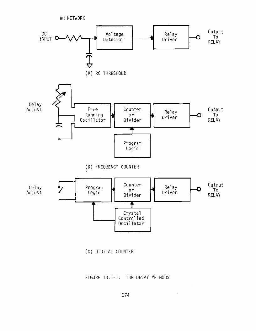
RC NETWORK
DC INPUT O — A A A
V Voltage Detector
(A) RC THRESHOLD
Relay Driver
Output — O To
RELAY
Delay Adjust Free
Running Oscillator
Counter or
Divider
Relay Driver
Output
— O To RELAY
(B) FREQUENCY COUNTER
Delay Adjust c Program
Logic
Counter or
Divider
Crystal Controlled Oscillator
Relay Driver
Output — O To
RELAY
(C) DIGITAL COUNTER
FIGURE 10.1-1: TDR DELAY METHODS
174
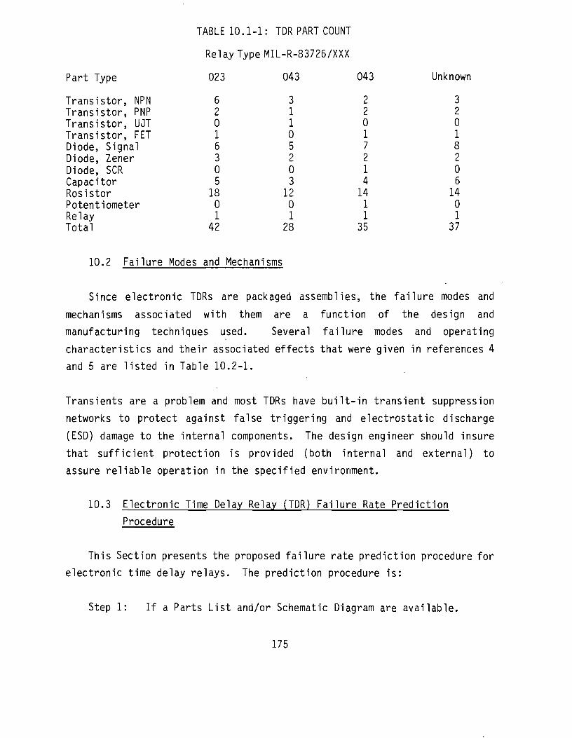
TABLE 10.1-1: TDR PART COUNT
Relay Type MIL-R-83726/XXX
Part Type
Transistor, NPN Transistor, PNP Transistor, UJT Transistor, FET Diode, Signal Diode, Zener Diode, SCR Capacitor Rosistor Potentiometer Relay Total
023
6 2 0 1 6 3 0 5 18 0 1 42
043
3 1 1 0 5 2 0 3 12 0 1 28
043
2 2 0 1 7 2 1 4 14 1 1 35
Unknown
3 2 0 1 8 2 0 6 14 0 1 37
10.2 Failure Modes and Mechanisms
Since electronic TDRs are packaged assemblies, the failure modes and
mechanisms associated with them are a function of the design and
manufacturing techniques used. Several failure modes and operating
characteristics and their associated effects that were given in references 4
and 5 are listed in Table 10.2-1.
Transients are a problem and most TDRs have built-in transient suppression
networks to protect against false triggering and electrostatic discharge
(ESD) damage to the internal components. The design engineer should insure
that sufficient protection is provided (both internal and external) to
assure reliable operation in the specified environment.
10.3 Electronic Time Delay Relay (TDR) Failure Rate Prediction
Procedure
This Section presents the proposed failure rate prediction procedure for
electronic time delay relays. The prediction procedure is:
Step 1: If a Parts List and/or Schematic Diagram are available.
175
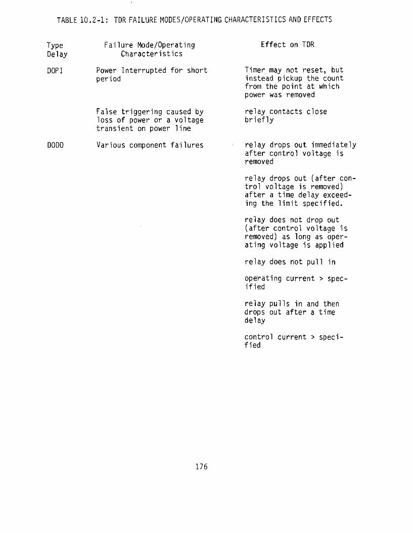
TABLE 10.2-1: TDR FAILURE MODES/OPERATING CHARACTERISTICS AND EFFECTS
Type Delay
DOPI
DODO
Failure Mode/Operating Characteristics
Power Interrupted for short period
False triggering caused by loss of power or a voltage transient on power line
Various component failures
Effect on TDR
Timer may not reset, but instead pickup the count from the point at which power was removed
relay contacts close briefly
relay drops out immediately after control voltage is removed
relay drops out (after control voltage is removed) after a time delay exceeding the limit specified.
relay does not drop out (after control voltage is removed) as long as operating voltage is applied
relay does not pull in
operating current > specified
relay pulls in and then drops out after a time delay
control current > specified
176
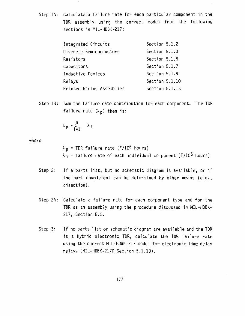
Step 1A: Calculate a failure rate for each particular component in the
TDR assembly using the correct model from the following
sections in MIL-HDBK-217:
Integrated Circuits Section 5.1.2
Discrete Semiconductors Section 5.1.3
Resistors Section 5.1.6
Capacitors Section 5.1.7
Inductive Devices Section 5.1.8
Relays Section 5.1.10
Printed Wiring Assemblies Section 5.1.13
Step IB: Sum the failure rate contribution for each component. The TDR
failure rate (Xp) then is:
where
^p =Ai ^ i i=l
X p = TDR failure rate (F/106 hours)
X-j = failure rate of each individual component (F/10^ hours)
Step 2: If a parts list, but no schematic diagram is available, or if
the part complement can be determined by other means (e.g.,
disect ion).
Step 2A: Calculate a failure rate for each component type and for the
TDR as an assembly using the procedure discussed in MIL-HDBK-
217, Section 5.2.
Step 3: If no parts list or schematic diagram are available and the TDR
is a hybrid electronic TDR, calculate the TDR failure rate
using the current MIL-HDBK-217 model for electronic time delay
relays (MIL-HDBK-217D Section 5.1.10).
177
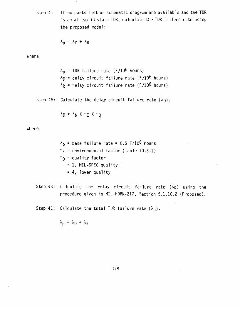
Step 4: If no parts list or schematic diagram are available and the TDR
is an all solid state TDR, calculate the TDR failure rate using
the proposed model:
xp = XD + XR
where
Xp = TDR failure rate (F/106 hours)
Xp = delay circuit failure rate (F/10^ hours)
XR = relay circuit failure rate (F/10^ hours)
Step 4A: Calculate the delay circuit failure rate (Xp)
XD = Xb X TTE X TTQ
where
X5 = base failure rate = 0.5 F/10^ hours
^E = environmental factor (Table 10.3-1)
TTQ = quality factor
= 1, MIL-SPEC quality
= 4, lower quality
Step 4B: . Calculate the relay circuit failure rate (XR) using the
procedure given in MIL-HDBK-217, Section 5.1.10.2 (Proposed).
Step 4C: Calculate the total TDR failure rate (X p).
Xp = XD + XR
178

TABLE 10.3-1: ENVIRONMENTAL FACTORS
Environment
%
GF
GM Mp
NSB NS Ny
NH NUU ARW
AlC AIT
AlB
TTE
1
4.5
16
12 8.4
8.8 20
18
20
26
8.8 12
35
Environment
AlA
AlF AUC AUT AlIB
AUA
ALIF
SF MFF MFA
USL ML
CL
TTE
18
30
15
21
58
33 52
0.58
12
17
35 40
680
10.4 Failure Rate Model Development
The approach utilized for model development was to treat the TDR as a
packaged assembly. The rationale for this approach is based on the following
facts:
o the TDR is a packaged assembly comprised of discrete components.
o every TDR is functionally a delay circuit and a switching circuit (relay); however, the circuit design and consequently the quantity, quality and type of components used in the design varies between manufacturers.
o The TDR MIL-SPEC is a functional specification and does not specify or limit internal construction.
However, it was recognized that it may not be possible for the reliability
analyst to obtain the parts list and/or schematic diagram for a TDR;
179

therefore a default prediction procedure was necessary. The following model
was hypothesized which could be used when limited data were available:
xp = XD + XR
where
Xp = TDR failure rate (F/106 hours)
Xp = delay circuit failure rate (F/106 hours)
X D = X b x TTE x TTQ
X b = base failure rate (F/106 hrs) (function of delay type (DOPI, DODO,
IT, etc.))
TTE = environmental factor
TTQ = quality factor
XR = relay failure rate (F/106 hours)
XR = MIL-HDBK-217D Section 5.1.10 for electromechanical relays
XR = MIL-HDBK-217D Section 5.1.10.2 (Proposed) for solid state relays
The TDR failure rate data collected in support of this study are
presented in Table 10.4-1. All of the data collected are for the hybrid DOPI
type TDR; therefore, although the type of delay is seen as having an affect
on reliability because each type requires a different complement of parts to
perform its function, separate X b factors could not be derived. A second
problem that arose from the data was that the failures cou1 I not be isolated
to a specific part; consequently, it could not be determined whether it was a
delay failure or a relay failure. The current MIL-HDBK-217 TDR failure rate
model was investigated to determine its applicability and accuracy. An
effort was undertaken to obtain the reliability predictions on the relays for
which data were obtained so that the accuracy of the prediction could be
checked. The predictions were not available. A second effort was initiated
to obtain the necessary technical information (temperature, no. of cycles,
stress ratio, etc.) from the applicable equipment technical orders. These
technical orders were not available either. It was then necessary to make
180

o i f i i f i i n n
o
0) t n i— + J J D I / 1 (O O L U CO i u"> i r*-. i i t — ( i i i i O J i n
• I • I • I I • I I I I • • CO i—t i—t r o ^ r i—t
X LT> O CO C^J L D i n O r o i ^ i t — i i i r o i i i i KO CO f—i * I > I « I I * I I I I > *
oo O O O «d" r-.
t o O H n o ^ c o o c M H H H i D n c M CNJ t—ICSJ l ^^DC^COCSJtXJ l ^ i ^D^ rCSJ t—I
N H n H i n o c f O H H H C J O O
O O ^ H O O O O O O O O O O ^ -
•>- N O M O r - i O O • — i O O O O « — i *X3
^-^fi-^ir^Srfff^.fJ d <0 '—* >> o en • 1 I I 1 I l OC Cd CH CH l •
o I t I I t I I I I I I I I
E O o> o I I I I
O U U U O I
Q) i—i * « -
> <IJ
-M O to dKD
CM
O O OJ *0 LO CD'CT' F— O 1- Q J Q I I UO |
II II II U -* - "O " ^ \ 3 z <o z: z: :
c_> •—i ct: z: <C ct: <c < i
I o o o Q Q Q I Q_ Q_ Q_ O- O- Q_
UO O O O O O H t v j f o r r Ln iD rscoo i
< m o o u j «—I t-H f—I f—I t—I I j r o ^ T L T ) i £ ) r - * . C 0 C T i - * - '
o
181

assumptions regarding the usage of the parts so that the accuracy of the
current model could be checked. The assumptions that were made are:
Source
1 thru 3 - Type = DPDT, temperature = 40°C, load = resistive, stress ratio = 0.75, cycling rate < 10/hour.
2 and 3 - Qual = MIL-SPEC
4 thru 7 - stress ratio = 0.75, cycling rate < 1/hour.
8 - load = resistive, stress ratio = 0.75, cycling rate < 10/hour.
These assumptions are for the most part reasonably accurate. The function of
most TDRs is to turn circuitry on or off after a preset delay. One would not
expect this to occur greater than once per hour on the average. The average
temperature for GF and Ns applications is approximately 23°C. The 40°C
assumption allows for a 17°C internal rise within the equipment and relay
enclosure. Source 2 and 3 are military equipments; therefore, it was assumed
that the parts used would be MIL-SPEC or equivalent. The stress ratio is the
recommended derated value for relays (reference 3). The assumption of a
resistive load was made sinCe the four points for which data were available
(source 4-7) were used with resistive loads. The assumption of a DPDT
configuration was made since five of the six points for which data were
available employed a DPDT configuration. The 75°C temperature assumption
for the ARW environment was made to be consistent with the other airborne
environments. It is probably a pessimistic assumption.
The data points for which all of the failure rate model parameters were
the same and which had zero failures recorded were merged. The predicted and
observed failure rates are given in Table 10.4-2. As can be seen, the data
does not disprove the accuracy of the current model. Therefore it is
proposed that the current model be retained as the default prediction method
for hybrid electronic TDRs.
182
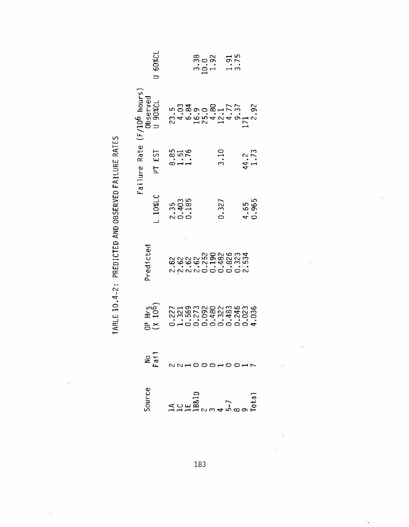
+-> fO
Ql
CD S-3
1— oo LU
1— Q_
LO ,—1 <£> o o i n r s COHH
C_J CO C\J t—I LO VS P O O O l O I N CD • • • • • I D ro o •—i •—i oo
(/) S- T3 3 (1) _ J o > c_j ro«d- O r ^ r ^ C%J
_c s- vs i n o c o o i o o o H s m en CD O
I D tncri ro«d-iD<jOLO«d-c\j«d-cr>.—IC%J 0 . 0 C\J i—i C\J r - i r»» r-H O => I—I Li_
</•> ^
LU
<: + J i— i D r H I D o ro Qi re oo co LO r»» i—i CM r% ~ C O H H ro «d-
<T3 Q L l _ LU C_J > _ i ro LO r»» Ln Q : )« inoco c-o in i£> LLJ o ro «d- I—i ro <JO cr> C/") i—I • • • • • • co M O O o «d- o O -J Q
< LLJ " O | _ CD u +-> cs jocs jv£>ro«d-i—i <J CsJCsJCsJCsJLOCTlCOCsJCsj rO Q -r- U O < J O I D I D C \ J . — i « d - c o r o L O 11 i "D • C£ CD CsJCsJCsJCsJOOOOOCsJ Q_ i-
CsJ I
2 </"£> rvHOlMCVJOCVJMlDMlO s - o csJcs jv r>r^c r i cocs jco«d-cs j ro
LU ZT. r-1 C s j r O L f ) C s J O « d - r O « d - C s J O O
C O Q- X O r - I O O O O O O O O " * < O ^
O -r-
LU C \ J C \ J r - l O O O i — l O O r - i r » »
CD U O c -S- r-H fO 3 oZ r^- +-> O CC C_J LU CO I O
</"> i—ii—ii—ii—icsjrO"^-Lr>cocri|—
183
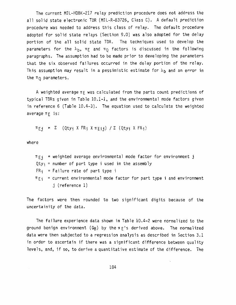
The current MIL-HDBK-217 relay prediction procedure does not address the
all solid state electronic TDR (MIL-R-83726, Class C). A default prediction
procedure was needed to address this class of relay. The default procedure
adopted for solid state relays (Section 9.0) was also adopted for the delay
portion of the all solid state TDR. The techniques used to develop the
parameters for the X^, TT£ and TTQ factors is discussed in the following
paragraphs. The assumption had to be made prior to developing the parameters
that the six observed failures occurred in the delay portion of the relay.
This assumption may result in a pessimistic estimate for Xb and an error in
the TTQ parameters.
A weighted average TTE was calculated from the parts count predictions of
typical TDRs given in Table 10.1-1, and the environmental mode factors given
in reference 6 (Table 10.4-3). The equation used to calculate the weighted
average Ti£ is:
TTEj = Z (Qtyi X FRi XTTEIJ) / 2 (Qtyi X FRi)
where
fr£j = weighted average environmental mode factor for environment j
Qty^ = number of part type i used in the assembly
FR-j = Failure rate of part type i
^Ei = current environmental mode factor for part type i and environment
j (reference 1)
The factors were then rounded to two significant digits because of the
uncertainity of the data.
The failure experience data shown in Table 10.4-2 were normalized to the
ground benign environment (Gg) by the TIE'S derived above. The normalized
data were then subjected to a regression analysis as described in Section 3.1
in order to ascertain if there was a significant difference between quality
levels, and, if so, to derive a quantitative estimate of the difference. The
184
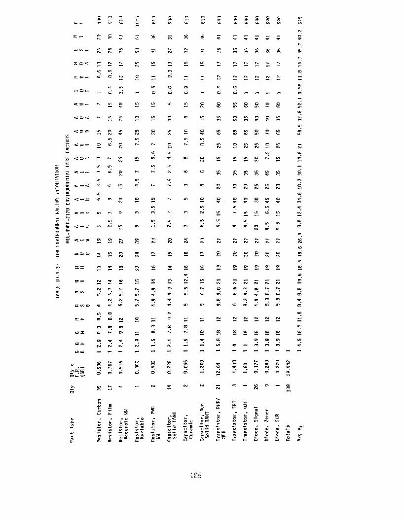
ZD V~) _ i ^ o - C M r~,
E: o i— cc cc
r-» r-»
CM CM CM CM CM CM
— © —
« = I D L - » ^
< : O <c r**
O K C lO
in in
=: «= — <
> < * - c s ȣ> Cr>
c i n*>
£ -
C C H U f : CM
i j ; x O". e n ^ — CM
* • « » -ty>
C M n*>
: :r> r> ^ m in co r»^
r** CTi
CM CM CM
g i f*- f"-
V CD CO
CD CO CO
r* ir, m
CD —
r*) c o CO
c c r»* e n co r^
C 3 L .
C2 CS
Cft ^ - * c
CM CM CM _ < ~ m
CM CM CM
CO CD CO
o d
— o » CM CM
o d d
~ < CM — \C Cn — CO
«<:
* o L. «— O X>
in — — fc.
«J =*•
#. L. O
tn
*r i CI I I
i - «C
« - t >
CL O fC */>
k-O U
~- E (J «3
C 0> fC L J
1 - <
o *-
u — »0 •—
c- o
o f t
£ c = !° £=.
185

source 2 and 3 data were deleted from the analysis because the quality level
of the parts could not be ascertained. The results of the regression are
shown in Table 10.4-4.
TABLE 10.4-4: TDR REGRESSION ANALYSIS RESULTS
Variable Coefficient (1) STD-Error F-Ratio
MIL-STD Quality (1.0)
Commercial Quality 1.4575 (4.3) 0.9875 2.18
Constant -1.865537 (0.155)
Notes: (1) Numbers in paranthesis are the transformed parameters
Quality was found to be significant at the 80% level. The proposed quality
factors (TTQ) are:
MIL-STD Quality 1
Commercial Quality 4
The factors were rounded to one significant digit because of the uncertainly
of the data.
The base failure rate factor (X^) was derived by taking the average value
of the upper 90% confidence bounds on the Table 10.4-2 source 1 and 4 through
8 data. The upper 90% confidence bounds were calculated for data normalized
to a MIL-SPEC part in a ground, benign environment. The average of the upper
90% confidence bounds was chosen to insure that an optimistic (lower than
what would actually be observed in the field 90% of the time) failure rate
was not predicted by the default technique. A secondary reason for using
this upper bound was to force the analyst to utilize one of the first two
techniques whenever possible since these techniques should generate a more
nearly accurate estimate of the true failure rate. The data from sources 2
and 3 were deleted from the analysis because the quality level of the part
could not be determined. The source 9 data were deleted because of the low
186

number of operating hours that were accumulated on the devices. The average
of the 90% confidence bounds is 0.464F/10^ hours. Due to the uncertainty in
the method of derivation, the base failure rate (Xt>) was rounded to 0.5 F/10^
hours.
10.5 References and Bibliography
References
1. Guth, George F., Development of Nonelectronic Part Cyclic Failure Rates, Martin Marietta Corporation, Final Technical Report, RADC-TR-77-417, December, 1977.
2. Arno, Robert G., Nonelectronic Parts Reliability Data, Reliability Analysis Center Publication NPRD-2, Summer, 1981.
3. I IT Research Institute, Electronic Reliability Design Handbook, Volume II, Contract Data Item, Contract F30602-78-C-0281, 1981.
4. Margolin, Bob, Time Delay Relays, DODOs, DOPIs and One-Shots, Electronic Products, May, 1979, pp 35-42.
5. Leach Relay Division, Technical Report, Failure Mode and Effects Analysis (FMEA) and MTBF Calculations, Leach Part No. TD-1161-1805, March, 1981.
6. Edwards, E., et.al., Avionic Environmental Factor's For MIL-HDBK-217, IIT Research Institute, Final Technical Report, RADC-TR-81-374, January, 1982.
Bibliography
Arno, Robert G., Nonelectronic Parts Reliability Data, Reliability Analysis Center Publication NPRD-2, Summer, 1981.
Daniels, Leocadia, Time Delay Relays, Electronic Products, March, 1982, pp. 57-60.
Edwards, E., et.al., Avionic Environmental Factors For MIL-HDBK-217, IIT Research Institute, Final Technical Report, RADC-TR-81-374, January, 1982.
Fink, Donald G., and Christiansen, Donald, Editors, Electronics Engineers' Handbook, Second Edition, McGraw-Hill, 1982.
187

Guth, George F., Development of Nonelectronic Part Cyclic Failure Rates, Martin Marietta Corporation, Final Technical Report, RADC-TR-77-417, December, 1977.
I IT Research Institute, Electronic Reliability Design Handbook, Volume II, Contract Data Item, Contract F30602-78-C-0281, 1981.
Leach Relay Division, Thermal and Electrical Stress Analysis Data, Orbiter EEE Part Application, Leach Part No. EPH-391, Relay, Hybrid Driver, General Purpose, March, 1980.
IBID., Reliability Stress Analysis, Time Delay Relay, Model TD-1505-2001.
IBID., Model TD-1827-2001.
IBID., Model TD-1161-1805.
IBID., Worst-Case Analysis, Model TD-1505-2001 Time Delay Relay.
IBID., Technical Report, Failure Mode and Effects Analysis (FMEA) and MTBF Calculations, Leach Part No. TD-1161-1805, March, 1981.
Margolin, Bob, Time Delay Relays, DODOs, DOPIs and One-Shots, Electronic Products, May, 1979, pp 35-42.
Rauch, Ed, Prevention of ESD Damage During the Manufacture of Time Delay Relays, Coping with Static Electricity, Part XXXI, Evaluation Engineering, July/August, 1982.
Southwest Research Institute, Nuclear Plant Reliability Data System, 1979 Annual Reports of Cumulative System and Component Reliability, December, 1979.
Yudewitz, Norman, Back to Relay Basics, Magnecraft Elec. *ic Company Pamphlet, 1980.
IBID., Prediction Relay Life Mathematically, Magnecraft Electric Company Pamphlet, 1980.
188

11.0 CIRCUIT BREAKERS
11.1 Part Description
The NEMA (National Electrical Manufacturers' Association) definition of
a circuit breaker is as follows: "A circuit breaker is a device for closing
and interrupting a circuit between separable contacts under both normal and
abnc-mal conditions. Normal indicates the interruption of currents not in
excess of the rated continuous current of the circuit breakers. Abnormal
indicates the interruption of currents in excess of rated continuous
currents such as short circuits. Ordinarily, circuit breakers are required
to operate relatively infrequently although some classes of breakers are
suitable for frequent operation."
The attributes of circuit breakers in general are that they open
automatically when required, are capable of carrying rated current and are
capable of switching rated current. A circuit breaker must accomplish four
fundamental duties:
(1) When closed it should be an ideal conductor.
(2) When open it should be an ideal insulator.
(3) When closed it must be able to interrupt its assigned current promptly without causing dangerous overvoltages.
(4) When open it has to be able to close promptly, possibly under short circuit conditions without contact welding.
Electromechanical circuit breakers considered in this study can be
broken down into three major categories; thermal, magnetic and thermal-
magnetic. Discussions of temperature compensated versions of thermal and
thermal-magnetic circuit breakers are also included in this section. Each
type of circuit breaker is available with one, two, three, four or more pole
configuration.
189
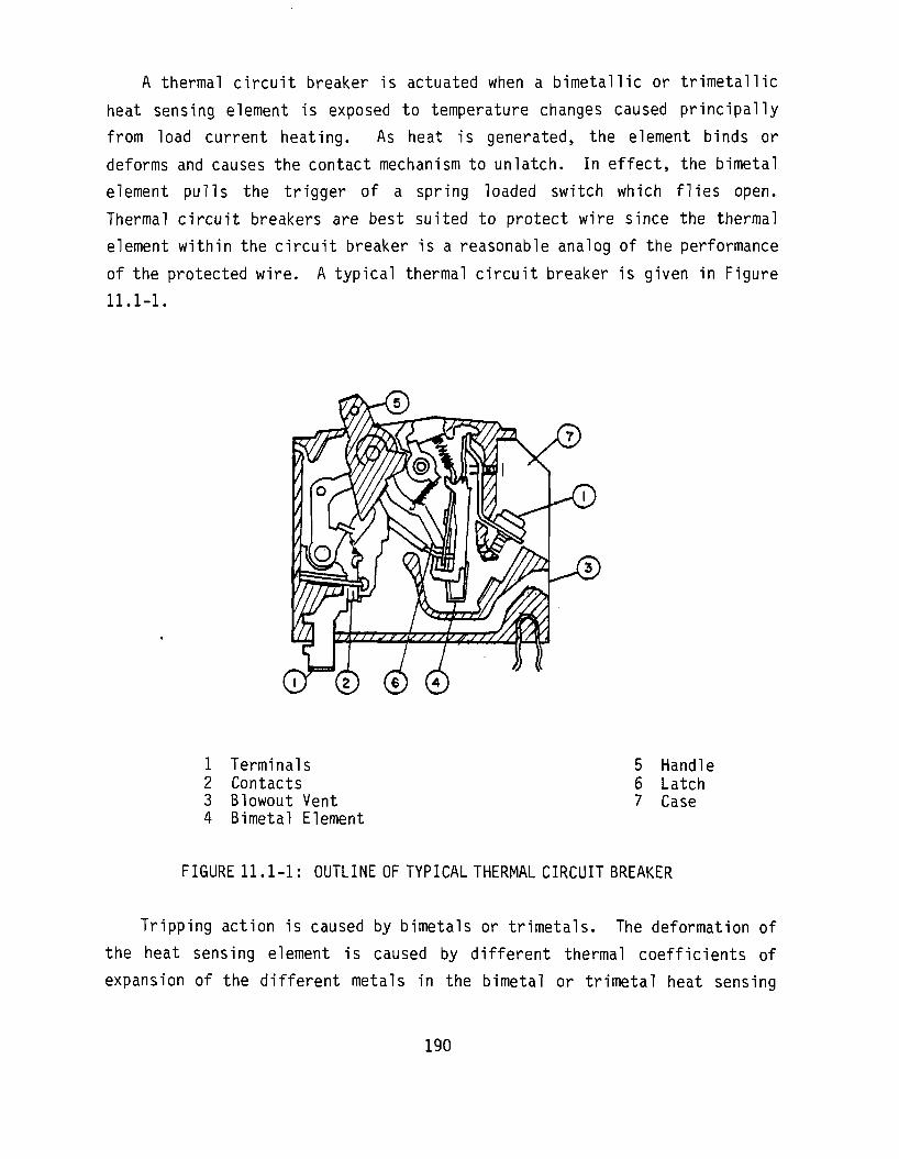
A thermal circuit breaker is actuated when a bimetallic or trimetallic
heat sensing element is exposed to temperature changes caused principally
from load current heating. As heat is generated, the element binds or
deforms and causes the contact mechanism to unlatch. In effect, the bimetal
element pulls the trigger of a spring loaded switch which flies open.
Thermal circuit breakers are best suited to protect wire since the thermal
element within the circuit breaker is a reasonable analog of the performance
of the protected wire. A typical thermal circuit breaker is given in Figure
11.1-1.
1 Terminals 5 Handle 2 Contacts 6 Latch 3 Blowout Vent 7 Case 4 Bimetal Element
FIGURE 11.1-1: OUTLINE OF TYPICAL THERMAL CIRCUIT BREAKER
Tripping action is caused by bimetals or trimetals. The deformation of
the heat sensing element is caused by different thermal coefficients of
expansion of the different metals in the bimetal or trimetal heat sensing
190

element. As relatively higher currents flow through the element, more heat
is generated and faster bending of the element occurs. One metal used for
the low expansion side of the element is invar. Copper is used in the center
of a trimetallic element for low resistivity. For high resistivity, nickel
is generally used. Various metals are used for the high expansion side.
Thermal circuit breakers have no instantaneous tripping point. A time
delay is associated with all tripping actions. A typical graph of tripping
time versus current overload is given in Figure 11.1-2. The actuation speed
of a thermal circuit breaker varies directly with temperature and with the
square of the current.
oo
O
oo
PERCENT OF RATED CURKLNT
FIGURE 11.1-2: TRIP TIME CHARACTERISTICS OF A TYPICAL
THERMAL CIRCUIT BREAKER
The deformation of the heat sensing element in thermal circuit breakers
is dependent on temperature change. The circuit breaker will trip regardless
of whether the temperature change is due to a current overload or a
combination of current overload and increase in ambient temperature. The
tripping time characteristics of thermal circuit breakers are highly
dependent on ambient temperature. Because of this fact temperature
compensated thermal circuit breakers are available. This type of circuit
191

breaker has an additional bimetal element which works in opposition to the
overload element. The opposition bimetal element is isolated from heat
generated by current overloads and therefore only deforms as a result of
increased ambient temperature.
Magnetic circuit breakers depend on changes in magnetic flux which are
caused by load current changes. The sensing and tripping functions are
performed by separate elements; the solenoid coil and the armature. Magnetic
circuit breakers contain a spring loaded movable iron core and a dampening
fluid in a nonmagnetic tube with a solenoid coil wound around. As current
increases, the iron core will move against the damping fluid because of
increased magnetic flux. As the iron core moves towards the armature, the
armature is attracted and the circuit breaker trips. If a critical magnetic
flux value is reached (at approximately 1000% rated current) then the
armature is attracted without movement of the iron core. This is the
instantaneous tripping point for magnetic circuit breakers. Figure 11.1-3
shows the construction of a typical magnetic circuit breaker.
Time delay for magnetic circuit breakers is provided by the action of the
fluid-damped movable iron core in the magnetic element. Overall delay
characteristics are determined by several design variables. The most
important design variable is the viscosity of the dampening fluid. Through
adjustment of these variables, virtually any time-delay curve (trip time
versus percent load) can be obtained. Ambient temperature has an effect on
the viscosity of the dampening fluid and therefore effects trip time
characteristics. Ambient temperature, however, has no effect on the
instantaneous tripping current value.
Magnetic breakers are employed in circuits having high in-rush currents.
A motor, for example, draws high current when power is first applied. As the
motor comes up to running speed, the current requirements drop off quickly to
normal. Because of the comparatively short duration of the high current
demands, most circuitry and equipment can safely tolerate them. Therefore,
it is not desirable to have circuit interruptions on these transient
192
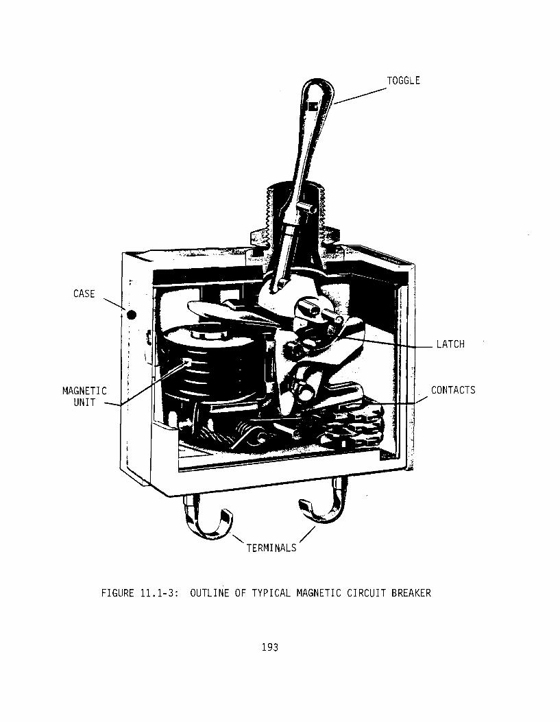
TOGGLE
CASE
MAGNETIC UNIT
LATCH
CONTACTS
TERMINALS
FIGURE 11.1-3: OUTLINE OF TYPICAL MAGNETIC CIRCUIT BREAKER
193
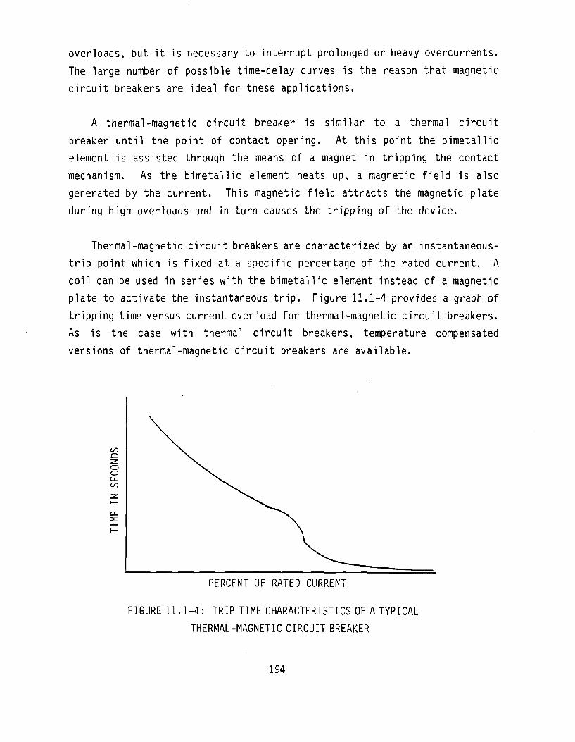
overloads, but it is necessary to interrupt prolonged or heavy overcurrents.
The large number of possible time-delay curves is the reason that magnetic
circuit breakers are ideal for these applications.
A thermal-magnetic circuit breaker is similar to a thermal circuit
breaker until the point of contact opening. At this point the bimetallic
element is assisted through the means of a magnet in tripping the contact
mechanism. As the bimetallic element heats up, a magnetic field is also
generated by the current. This magnetic field attracts the magnetic plate
during high overloads and in turn causes the tripping of the device.
Thermal-magnetic circuit breakers are characterized by an instantaneous-
trip point which is fixed at a specific percentage of the rated current. A
coil can be used in series with the bimetallic element instead of a magnetic
plate to activate the instantaneous trip. Figure 11.1-4 provides a graph of
tripping time versus current overload for thermal-magnetic circuit breakers.
As is the case with thermal circuit breakers, temperature compensated
versions of thermal-magnetic circuit breakers are available.
Q
O O
PERCENT OF RATED CURRENT
FIGURE 11.1-4: TRIP TIME CHARACTERISTICS OF A TYPICAL
THERMAL-MAGNETIC CIRCUIT BREAKER
194

For each type of circuit breaker trip free construction is required in
most applications. With this construction, the contact arm is independent of
the manual operating handle while a fault exists. It is impossible to hold
the contacts manually closed against an overload or short circuit. There are
applications, primarily in aircraft operation, where a nontrip-free
construction is desirable. These are cases where the function performed by
the equipment is more important than the equipment itself; in these cases,
non-trip-free construction permits the contacts to be held closed manually
against the fault.
As can be deduced from this section, there are two basic means of circuit
interruption for circuit breakers; thermal and magnetic. The use of a
bimetal or trimetal heat sensing element is the distinguishing
characteristic between the two basic types.
11.2 Failure Modes and Mechanisms
The failure modes and mechanisms for circuit breakers are similar to
those of other electromechanical devices such as relays and switches.
Reference 1 provides a failure mode distribution for circuit breakers in
general, which is presented in Table 11.2-1.
TABLE 11.2-1: CIRCUIT BREAKER FAILURE MODE DISTRIBUTION
FAILURE MODE FREQUENCY OF OCCURENCE
SHORT 38%
OPEN 38%
UNSTABLE 19%
ARCING 5%
All electromechanical devices such as circuit breakers would be expected
to exhibit wearout type failures. Examples of possible wearout failure
195
mechanisms for circuit breakers are (1) fatigue induced failures of the
bimetal element in thermal circuit breakers, (2) relaxation of the spring
constant of springs used in circuit breakers, (3) contact surface
degradation and (4) mechanical wear on moving parts. These wearout failure
mechanisms would suggest that the failure rate of circuit breakers is an
increasing function of time. However, empirical data to support this
hypothesis is nonexistent. It cannot be determined whether the hazard rate
of circuit breakers differs significantly from a constant value over the
expected life of the equipment in which they are installed. Therefore until
such data becomes available, the hazard rate of circuit breakers should be
assumed constant.
All types of circuit breakers are susceptible to failures induced by
environmental stress. Several different failure mechanisms which are
accelerated by the environment are discussed in the following paragraphs.
At high altitudes contact arcing can occur at lower voltages and last
longer as the contacts separate. This is mainly due to the fact that the
dielectric strength of the air tends to decrease as barometric pressure
decreases. Therefore when circuit breakers are used in high altitude
applications, derated load and life specifications should be applied.
Insulating materials found in some circuit breakers may absorb moisture
which decreases insulation resistance. Moisture may also condense on
contact surfaces in a high humidity application and promote contact
corrosion or galvanic action. Therefore, the selection of insulating
material is important if the circuit breaker is to be applied in a high
humidity environment.
In circuit breakers that use lubricants in bearing areas, high ambient
temperatures may cause the flow of the lubricant onto the contacts or
insulating surface. The reduction of lubrication on the moving parts may
accelerate the wear of mechanical parts. Any film of lubricant deposited on
196

the insulating surfaces can capture dust and particles that reduce the
dielectric strength and insulation resistance.
Very low ambient temperatures can decrease the viscosity of the
lubricant and result in slower switching speed or even incomplete contact
closure. Under certain atmospheric conditions ice may form causing higher
and varying contact resistance. Increased contact forces tend to eliminate
these problems.
Circuit breakers are more susceptible than switches to failure of the
actuating mechanism. The actuating mechanisms in circuit breakers are not
only more complex but are also susceptible to wear and fatigue from high
impact loads. Incorrect operating and release forces are the main cause of
failure. Premature switching or failure to switch may be due to mechanical
misalignment of the actuation members, contamination, loose or defective
parts, corrosion, or excessive wear on parts improperly installed.
A factor which obviously effects the reliability of circuit breakers is
the configuration. A more complex circuit breaker (i.e. four pole) would be
expected to have a higher failure rate than a less complex circuit breaker
(i.e. one pole). This has been documented for other electromechanical
devices (relays, switches) in MIL-HDBK-217D.
Poor manufacturing processes may also play an important role in the
failure mechanisms of circuit breakers. Such anomalies as deformed
contacts, loose or broken contacts, termination separation, and some
external mechanisms may cause early failure of the circuit breaker. Loose or
broken contacts are in many cases caused by inadequate welding of the leader,
frame or support bracket. Shock or vibration can induce failures.
Termination separation is the result of inadequate wire or terminal routing
clearance. This can result in actuation mechanism interference, sharp bend
radii resulting in the breakage of the wire, defective solder joints,
overstressed solder joints, or defective welds. Failure mechanisms of this
type can be eliminated by a thorough incoming inspection.
197

11.3 Circuit Breaker Failure Rate Prediction Model
This section presents the proposed failure rate prediction model for
circuit breakers. The proposed model is:
Xp = Xb ire Q E
where Xp = predicted circuit breaker failure rate
Xb = base failure rate
= 0.020 failures/106 hours, magnetic circuit breakers
= 0.038 failures/10^ hours, thermal circuit breakers
= 0.038 failures/10^ hours, thermal-magnetic circuit breakers
TTC = configuration factor (see Table 11.3-1)
TTQ = quality factor
= 1.0, MIL-SPEC quality
= 8.4, lower quality
IT £ = environmental factor (see Table 11.3-2)
TABLE 11.3-1: CONFIGURATION FACTOR
Configuration
SPST
DPST
SPDT
3PST
4PST
DPDT
3PDT
4PDT
6PDT
• TTC
1.00
1.50
1.75
2.00
2.50
3.00
4.25
5.50
8.00
198

TABLE 11.3-2: ENVIRONMENTAL FACTOR
Environment
GB
GF
6M
Mp
NSB NS Nu
NH
NUU
ARW
AlC AIT
AlB
TTE
1.0
2.3 8.2
21
7.9
7.9 14
32 34
46
6.0
5.5
10
Environment
AlA
AlF AUC AUT AlIB
AUA
AUF
SF MFF
MFA
USL
ML
CL
TTE
7.!
10 9.1
8.1
15
10
15
l.i
21
29
62
71
N/A
11.4 Failure Rate Model Development
The approach utilized for model development was to identify significant
parameters by analysis of circuit breaker field experience failure rate
data. The model parameters were then quantified using the same data. At the
conclusion of each step, the results were given i thorough analysis to
determine whether they were consistent with theory. The circuit breaker
failure rate data collected in support of this study is presented in Table
11.4-1. Data entries with zero failures and less than 500,000 part hours
were merged with other data which were similar in regard to quality level,
type, configuration and environment.
Application and construction variables were identified for circuit
breakers and presented in Table 11.4-2. The application and construction
variables represent factors which were determined whenever possible for all
collected data. If sufficient detail could not be determined for a
199

particular data entry, then it was not included in the model development
process.
Theoretically the circuit breaker configuration is a significant
variable effecting failure rate. To supplement the available data, the
relation between configuration and failure rate was analyzed for other
electromechanical devices with construction similarities to circuit
breakers. The MIL-HDBK-217D failure rate prediction models for switches and
relays include an identical factor based on device configuration. It was
assumed that a configuration factor for circuit breakers would have a similar
form. The factor for relays and switches is defined by the following
equation.
TTC = 0.75PT - 0.25P + 0.50
where
" c = device configuration factor
P = quantity of poles
T = quantity of throws
Assuming that the circuit breaker failure rate is best represented by a
multiplicative model (i.e. ^p = \ ^i " 2-••)» inclusion of a factor in the
form of the device configuration factor results in a nonlinear equation. As
described in Section 3.1 regression analysis is difficult when the assumed
model format is nonlinear. To solve this problem, the configuration factor
which is applied to switches and relays was temporarily assumed to be correct
for circuit breakers.
At the conclusion of the regression analysis, this assumption was examined to
determine its feasibility.
200

lAbLL 1 1 . 4 - 1 : URCU11 BRLM'.U FAILURl UAH 0A1A
ENTRI NO.
1 2 (1 ) 3 (1 ) 4 (1 ) 5 6 ( 1 ) 7 ( 1 ) 8 (1 ) 9 ( 1 )
10 ( 1 ) 11 (1 ) 12 (1 ) 13 (1 ) 14 15 (1 ) 16 (1 ) 17 (1 ) 18 (1 ) 19 ( 1 ) 20 (1 ) 21 (1 ) 22 ( 1 ) 23 (1 ) 24 (1 ) 25 (1 ) 26
27 (1 ) 28 ( 1 ) 29 30 31 (1 ) 32 ( 1 ) 33 ( 1 ) 34 (2 ) 35 (2 ) 36 (2 ) 37 (2 ) 38 ( 1 ) 39 ( 1 ) 40 ( 1 ) 41 42 (1 ) 43 (1 ) 44 45 46 47 48 49 50 51 52 53 54 55 56 57 58 59 (1 ) 60 ( 1 ) 61 (2 ) 62 (2 ) 6.3 ( 2 ] 64 (2 ) 65 ( 2 ) 66 (2 ) 67 (2 ) 68 (2 ) 69 70
OUALlTi
HU-SPtC HlL-SPtC MIL-SPEC MIL-SPEC MIL-SPEC MIL-SPEC MIL-SPEC MIL-SPEC MIL-SPEC MIL-SPEC MIL-SPEC MIL-SPEC MIL-SPEC MIL-SPEC MIL-SPEC MIL-SPEC MIL-SPEC HIL-SPEC H1L-SPEC MIL-SPEC MIL-SPEC MIL-SPEC MIL-SPEC MIL-SPEC MIL-SPEC MIL-SPEC MIL-SPEC MIL-SPEC Conmercia Conmercia Commercia Coirmercia Conmercia Conmercia Commercia Conmercia Coirmercia Conmercia Conmercia Conmercia Conmercia Conmercia Commercia Conmercia Conmercia Conmercia Conmercia Commercia Conmercia Conmercia Conmercia Conmercia Conmercia Commercia Conmercia Conmercia Conmercia Conmercia Conmercia Conmercia Conmercia
( 4 )
w ( 4 ) ( 4 ) (4 ) ( 4 ) ( 4 )
Conmercia Conmercia
TYPE
Magnetic Magnetic Magnetic Magnetic Magnetic Magnetic Magnetic Magnetic Magnetic Magnetic Magnetic Magnetic Magnetic Magnetic Magnetic Magnetic Magnetic Magnetic Magnetic Magnetic Magnetic Magnetic Magnetic Magnetic Magnetic Magnetic Magnetic Magnetic Magnetic Magnetic Magnetic Magnetic Magnetic Magnetic Magnetic Magnetic Magnetic Magnetic Magnetic Magnetic Magnetic Magnetic Magnetic Thermal Thermal Thermal Thermal Thermal Thermal Thermal Thermal Thermal Thermal Thermal Thermal Thermal Thermal Thermal Thermal Thermal
( 4 ) ( 4 ) ( 4 ) (4 ) (4 ) ( 4 ) ( 4 ) ( 4 )
Under V o l t . Under V o l t .
CONFIGURATION
3PST DPST SPST SPST 3PST SPST SPST SPST SPST SPST SPST SPST SPST DPST 3PST 3PST 3PST DPST DPST DPST DPST DPST DPST SPST SPST 3PST DPDT 3PST SPST DPDT SPST 3PST 3PST (4 ) ( 4 ) ( 4 ) ( 4 ) SPST SPST SPST OPST 3PST 3PST SPST OPST 3PST 3PST 3PST 3PST 3PST 3P.ST 3PST 3PST SPST DPST 3PST 3PST 3PST 3PST 3PST ( 4 ) ( 4 ) ( 4 ) ( 4 ) ( 4 ) ( 4 ) ( 4 ) ( 4 ) ( 4 ) ( 4 )
ENVIRONMENT
GF
Gr GF GF NS8 GM GM GM GM GH GM GM GM GM GM GM GH GF GF GF GF GF GF GF GF GF GF GM GF GM GF GF GF GF GF GF GF GF GF GF GM GM GM GF GF GF GF GF GF GF GF GF GF GF GF GF GF GF GF GF Al AIF GM GF GF SF NS NS GF GF
TEMT (°C)
25 ( 4 ) 25 25 45 30 30 30 30 3D 30 30 30 30 30 30 30 (4 ) ( 4 ) ( 4 ) ( 4 ) ( 4 ) ( 4 ) (4 ) ( 4 ) (4 ) ( 4 ) ( 4 ) 25 30 (4 ) (4 ) ( 4 ) ( 4 ) ( 4 ) ( 4 ) (4} 25 25 25 30 30 30 (4 ) ( 4 ) ( 4 ) ( 4 ) ( 4 ) ( 4 ) ( 4 ) (4 ) ( 4 ) ( 4 ) ( 4 ) ( 4 ) ( 4 ) ( 4 ) ( 4 ) ( 4 ) ( 4 ) ( 4 ) ( 4 ) ( 4 ) ( 4 ) ( 4 ) ( 4 ) ( 4 ) (4 ) (4 ) ( 4 )
PART NO.
M 9 0 1 9 / 5 M39010/4 M39019/1 M390I0 /1 M39019/5 M39019/1 M39019/1 M39019/1 M39019/1 M39019/1 M39019/1 M39019/1 M39019/1 M39019/3 M39019/5 M39019/5 M39010/5 M55629/4 H55629/4 M55629/4 M55629/4-H55629/3-M55629/3-H55629/2-M55629/2-M55629/5-M55629/3-M55629/5-
(3 ) ( 3 ) ( 3 ) (3 ) (3 ) ( 3 ) ( 3 ) ( 3 ) ( 3 ) ( 3 ) ( 3 ) ( 3 ) ( 3 ) ( 3 ) ( 3 ) ( 3 ) ( 3 ) ( 3 ) ( 3 ) (3 ) ( 3 ) ( 3 ) ( 3 ) ( 3 ) (3 ) ( 3 ) ( 3 ) ( 3 ) ( 3 ) ( 3 ) ( 3 ) ( 3 ) ( 3 ) ( 4 ) ( 4 ) ( 4 ) ( 4 ) ( 4 ) ( 4 ) ( 4 ) ( 3 ) ( 3 )
70 47 218 248 70 215 218 225 228 231 242 249 258 200 200 230 249 039 046 067 095 102 130 46 107 08 116 132
EQUIPMENT
AN/UYK-7 AN/EPS-108 AN/Grq-18 AN/GYQ-18 AN/UYK-7 AN/TSO-73 AN/TSO-73 AN/TSO-73 AN/TSO-73 AN/TSO-73 AN/TSO-73 AN/TSO-73 AN/TSO-73 AN/TSO-73 AN/TSO-73 AN/TSO-73 AN/TSO-73 AN/FPS-108 AN/FPS-108 AN/FPS-108 AN/FPS-108 AN/FPS-108 AN/FPS-108 AN/FPS-108 AN/FPS-108 AN/FPS-108 AN/FPS-108 AN/TSO-73 AN/GYO-18 AN/TSO-73 AN/FPS-108 AN/FPS-108 AN/FPS-108 AN/FPS-108 AN/FPS-108 AN/FPS-108 AN/FPS-108 AN/GYO-18 AN/GrQ-18 AN/GYO-18 AN/TSO-73 AN/TSO-73 AN/TSO-73
(4 ) ( 4 ) ( 4 ) ( 4 ) ( 4 ) ( 4 ) ( 4 ) ( 4 ) ( 4 ) ( 4 ) (4 ) ( 4 ) ( 4 ) ( 4 ) ( 4 ) ( 4 ) ( 4 ) ( 4 ) ( 4 ) (4 ) ( 4 ) ( 4 ) ( 4 ) ( 4 ) ( 4 ) ( 4 ) ( 4 )
FAILURES
1 0 0 0 1 0 0 0 0 0 0 0 0 0 0 0 0 0 0 0 0 0 0 0 0 0 0 0 0 0 0 0 0 0 0 0 0 0 0 0 0 0 0 1 2 0 2 3 0 1 1 2 3
10 6 2 2 0 0 0 0
236 30
2 61
4 1 0 8 D
PARI HOIIi ',
1U.7U/.U0U 2B.51?
305. 'JO? 355.1102 111.ODD 123,000 246.000 123.000 246,000 123,000 123.000 123.000 123,000 123,000 246,000 246,000 369,000
28.51? 28,512 28.512 28.51?
142,560 28,512 28.512 28,512 28.512
114,048 123,000
1,067,706 3.690,000
28,512 28,512 28,512 28.512 28,512 28.512 28,512
355,90? 355,902 355,902 123,000 123,000 246,000
3 ,211 ,200 3 ,211.200 1,090,080 1.090.080 3 ,504 ,000 1,477,520
350,400 425,088 8?9,440 8?9,440
3.818,016 3 ,181 .680 1,487,808 1.91?,896 1,062,720
363,360 425,088
17,200 119,998,000 39,708,000
20 ,340 ,970 88 ,109 .000
8 ,872 ,000 1,215,000 2 ,522 ,488 3 .504 ,000
744,000
NOTES:
(1) Data merged with other data entries of similar quality, (2) Use of data questionable due to lack of detail. (3) Commercial part numbers are proprietary. (4) Unknown.
type, configuration and environment.
201
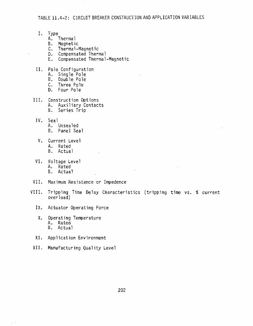
TABLE 11.4-2: CIRCUIT BREAKER CONSTRUCTION AND APPLICATION VARIABLES
I. Type A. Thermal B. Magnetic C. Thermal-Magnetic D. Compensated Thermal E. Compensated Thermal-Magnetic
II. Pole Configuration A. Single Pole B. Double Pole C. Three Pole D. Four Pole
III. Construction Options A. Auxiliary Contacts B. Series Trip
IV. Seal A. Unsealed B. Panel Seal
V. Current Level A. Rated B. Actual
VI. Voltage Level A. Rated B. Actual
VII. Maximum Resistance or Impedence
VIII. Tripping Time Delay Characteristics (tripping time vs. % current overload)
IX. Actuator Operating Force
X. Operating Temperature A. Rated
B. Actual
XI. Application Environment
XII. Manufacturing Quality Level
202

Stepwise multiple linear regression analysis as described in Section 3.1
was applied to the circuit breaker failure rate data normalized by the
assumed configuration factor. The data entries in Table 11.4-1 which
included both sufficient detail and sufficient part hours to apply
regression analysis are entry numbers 1, 29, 30, 44, 45, 46, 47, 48, 49, 50,
51, 52, 53, 54, 55, 56, 67 and 58. The regression analysis resulted in the
following failure rate prediction model.
Xp = Xb TTC TTQ
where
Xp = circuit breaker failure rate in failures/10^ hours
Xb = base failure rate
= 0.0450 failures/10^ hours, magnetic circuit breakers
= 0.0884 failures/10^ hours, thermal circuit breakers
TTC = configuration factor
TTQ = quality factor
= 1.0, MIL-SPEC
= 8.41, lower quality
It should be noted that the base failure rate values given above differ from
the base failure rate values given in Section 11.3. This discrepancy is
explained later in this section where environmental factors are introduced.
The details of the regression analysis are given in Table 11.4-3. Base
failure rate and quality factor were defined by the following equations. Xi
and X2 are "dummy variables" used to quantify qualitative factors such as
quality level and circuit breaker type.
Xb = exp (constant + biXi)
Xi = 0, magnetic circuit breakers
X} = 1, thermal circuit breakers
TTQ = exp (b2X2)
X2 = 0, MIL-SPEC
X2 = 1 , lower qua l i t y
203
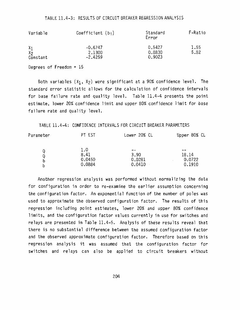
TABLE 11.4-3: RESULTS OF CIRCUIT BREAKER REGRESSION ANALYSIS
Variable Coefficient (b-j) Standard F-Ratio Error
Xi -0.6747 0.5427 1.55 X2 2.1300 0.8830 5.82 Constant -2.4259 0.9023
Degrees of Freedom = 15
Both variables (X]_, X2) were significant at a 90% confidence level. The
standard error statistic allows for the calculation of confidence intervals
for base failure rate and quality level. Table 11.4-4 presents the point
estimate, lower 20% confidence limit and upper 80% confidence limit for base
failure rate and quality level.
TABLE 11.4-4: CONFIDENCE INTERVALS FOR CIRCUIT BREAKER PARAMETERS
Parameter PT EST Lower 20% CL Upper 80% CL
3.90 18.14 0.0281 0.0722 0.0410 0.1910
Another regression analysis was performed without normalizing the data
for configuration in order to re-examine the earlier assumption concerning
the configuration factor. An exponential function of the number of poles was
used to approximate the observed configuration factor. The results of this
regression including point estimates, lower 20% and upper 80% confidence
limits, and the configuration factor values currently in use for switches and
relays are presented in Table 11.4-5. Analysis of these results reveal that
there is no substantial difference between the assumed configuration factor
and the observed approximate configuration factor. Therefore based on this
regression analysis it was assumed that the configuration factor for
switches and relays can also be applied to circuit breakers without
Q Q b b
1.0 8.41 0.0450 0.0884
204

introducing error. The equation determined from the data to approximate the
configuration factor is:
TTC = 0.857 exp (0.154 P)
where P = quantity of poles
TABLE 11.4-5: CONFIGURATION FACTOR ANALYSIS
observed configuration factors assumed factors Configuration ITCJ o.20 *c ^c, 0.80 IT,
SPST 0.8 1.0 1.3 1.0 DPST 0.8 1.2 1.8 1.5 3PST 0.7 1.4 2.7 2.0
The assumed configuration factor was deemed preferable to the observed
approximate configuration factor for several reasons. The assumed factor is
an established documented factor and therefore should not be altered without
substantial proof that it is inaccurate. The assumed factor was derived
using data with higher pole configurations than was available for this study
effort. If circuit breaker failure rate data could have been obtained with
four or more poles, then the assumed and observed factors could have been
aligned more precisely. Additionally, it was felt that the derivation of an
additional factor based solely on the available data entries may have placed
too high a burden on the available data and increased the probability of
modeling "statistical noise".
Environment was not identified as a significant variable in the
regression analysis. This does not imply, however, that environment is not a
significant factor effecting reliability. The environment was omitted
because the data used in the regression analysis was primarily from the
ground fixed and ground mobile environment categories. The data collected in
space flight, naval sheltered and air inhabited fighter environment
categories was not used because sufficient detail regarding the circuit
breakers was not obtainable. Theoretically, environmental stress has a
205

great effect on reliability and therefore an alternate approach was
developed to derive a series of environmental factors.
The approach used to develop the environmental factors included
comparison of circuit breaker failure modes and mechanisms with those of
other electromechanical devices, primarily switches and relays. The
anticipated effect of environmental stress on contact life, accelerated
mechanical wear on moving components and other factors suggest similar
environmental factors. The existing MIL-HDBK-217D environmental factors for
relays, switches and connectors are given in Table 11.4-6. Relays and
connectors each have two series of environmental factors depending on
quality level.
TABLE 11.4-6: ENVIRONMENTAL FACTORS OF ELECTROMECHANICAL PARTS
Relays Relays (Lower Connectors Connectors
Environment
GB SF GF NSB NS AIT Mp MFF MFA GM NH NUU AUT Nu AlF ARW USL AUF ML cL
(MIL-SPEC)
1 1 2.3 8 8 4.0 2-1 21 29 8.2 32 34 12 14 8.0 46 62 24 71 N/A
Quality)
2 (2.0) 4.6 24 24 8.0 63 63 82 25 96 100 30 38 16 140 190 60 210 N/A
Switches
1 1 2.9 7.9 7.9 5 21 21 29 14 32 34 50 20 10 46 63 100 71
1200
(MIL-SPEC)
1 1 1.2 4.1 5.3
• 5.0 8.5 8.5 12 8.3 13 14 5 13 10 19 25 10 29 490
(Lower Q
1 1 4 8 11 15 17 17 24 25 26 28 15 27 30 37 50 30 58 970
All data with recorded failures were merged according to environment to
generate the environmental factors for circuit breakers. These data are
206

presented in Table 11.4-7. The failure rates given in Table 11.4-7 represent
average values with respect to type, configuration and quality level. In
order to use these data in conjunction with the existing environmental
factors for electromechanical devices, a Chi-squared test was run to
determine which of the five series of environmental factors given in Table
11.4-6 best represent the effect of environmental stress on circuit
breakers. The Chi-squared test was set up with the average failure rates
given in Table 11.4-7 equal to the observed values in the test and a series
of predicted failure rates (as a function of the environmental factors given
in Table 11.4-6) equal to the predicted values. The predicted failure rate
value as a function of chosen environmental factor is given by,
X p r e = (2X0bs/E7T£)lTE
where
Xp r e = predicted average failure rate
X0bs = observed average failure rate (Table 11.4-7)
TTJ: = environmental factor (Table 11.4-6)
This equation gives a best fit between observed and predicted values for each
series of environmental factors given in Table 11.4-6. Then the Chi-squared
test was applied to determine the optimal series of environrental factors. A
brief discussion of the Chi-squared test is given in Sect on 3.1.
TABLE 11.4-7: CIRCUIT BREAKER FAILURE RATE DATA MERGED BY ENVIRONMENT
Environment No. of Failures Part hours(xl06) Failure Rate (f/106hours)
SF 4 8.872 0.451 GF 107 146.519 0.730 GM 30 39.708 0.756 NS 1 1.215 0.823 AIF 236 119.998 1.967
207
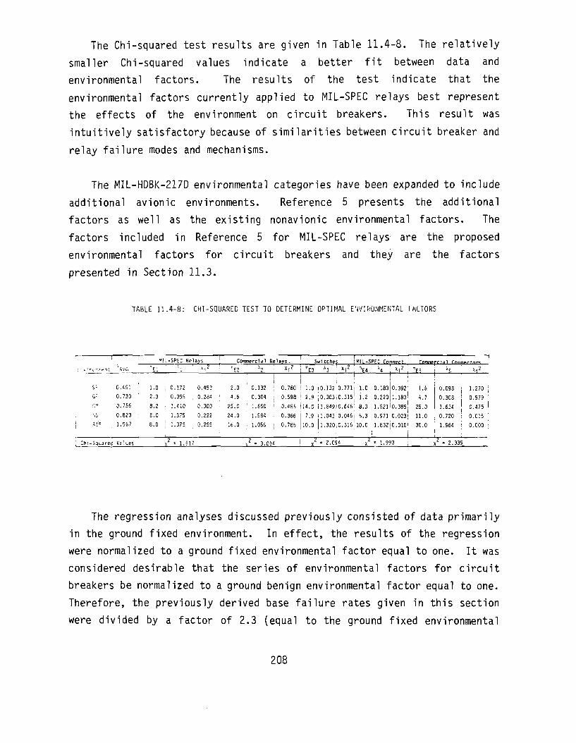
The Chi-squared test results are given in Table 11.4-8. The relatively
smaller Chi-squared values indicate a better fit between data and
environmental factors. The results of the test indicate that the
environmental factors currently applied to MIL-SPEC relays best represent
the effects of the environment on circuit breakers. This result was
intuitively satisfactory because of similarities between circuit breaker and
relay failure modes and mechanisms.
The MIL-HDBK-217D environmental categories have been expanded to include
additional avionic environments. Reference 5 presents the additional
factors as well as the existing nonavionic environmental factors. The
factors included in Reference 5 for MIL-SPEC relays are the proposed
environmental factors for circuit breakers and they are the factors
presented in Section 11.3.
TABLE 11.4-8: CHI-SQUARED TEST TO DETERMINE OPTIMAL ENVIRONMENTAL fACTORS
i
: • . • iv rven i
Sc
G =
GM
:.S
^!F
CMi-Squared
!
0 .45!
0.730
0.756
0.623
1.967
Values
M
" ^ l
1.0
2.3
8.2
E.O
8.0
L-SPEC Relays
' l ' M 2
; 0.172 0.153
• 0.395 , 0.284
; 1.410 . 0.303
1.375 0.222
| 1.375 0.255
»2 = 1.517
Conmercial
"E2
2.0
4.6
25.0
24.0
16.0
,s2
i 0.132
0.304
j 1.650
1.584
I 1.056
Rel
I
j
1
i
i
v2 • 3.014
a y s .
* i 2
0.780
0.596
0.485
0.366
0.785
Switches
*E3 A3 ! " I 2
1.0 i0.13210.771
2.9 ;0.3e3J0.315
14.0 11.84910.646
7.9 1.043 0.046
10.0 11.320i0.316 j :
/ - 2.094
" — 1 MIL-SPEC Connect.^
*E4 ! x4 : * i 2 ;
1.0 10.183
1.2 !0.220
8.3 |1.521
0.392'
1.163
0.385;
5.3 |0.971 0.023
10.0 1.83210.0101
l
x ' - 1.993
1
'E5
1.5
4.7
25.0
11.0
30.0
h !
0.096 j
0.306
1.634
0.720
1.964 ;
<Z • 2.339
h2
1.270 :
0.579 :
0.475 1
0 . 0 1 5 J 0.000 i
1 \
The regression analyses discussed previously consisted of data primarily
in the ground fixed environment. In effect, the results of the regression
were normalized to a ground fixed environmental factor equal to one. It was
considered desirable that the series of environmental factors for circuit
breakers be normalized to a ground benign environmental factor equal to one.
Therefore, the previously derived base failure rates given in this section
were divided by a factor of 2.3 (equal to the ground fixed environmental
208

factor). This could be done because of the multiplicative nature of the
circuit breaker failure rate prediction model. The normalized base failure
rates are as follows:
XD = base failure rate
= 0.0196 failures /10& hrs, magnetic circuit breakers
= 0.0384 failures /10^ hrs, thermal circuit breakers
These values for base failure rate are identical to the base failure rate
values given in Section 11.3 except for the number of significant digits. No
failure rate data was available for thermal-magnetic circuit breakers.
Based on theoretical considerations, the base failure rate developed for
thermal circuit breakers was also applied to thermal-magnetic circuit
breakers. The underlying factor was the use of a bimetal or trimetal heat
sensing element to initiate tripping of the circuit breakers.
The determination of appropriate environmental factors and the
normalization of the base failure rate values concludes the circuit breaker
model development procedure. The development of modifying factors based on
circuit breaker type, quality level, configuration and environment will
greatly enhance failure rate prediction capabilities for these complex
electromechanical devices.
11.5 References
1. Arno, R.G. (I IT Research Institute, Rome NY). Nonelectronic Parts Reliability Data, NPRD-2. Summer 1981.
2. Davis, W.B. (Airpax, Cambridge, MD). The Choice of Protection, 1979.
3. Machine Design, May 19, 1977, pp. 132-156.
4. Machine Design, May 13, 1982, pp. 139-146.
5. Edwards, E., Flint, S. and Steinkirchner, J. (I IT Research Institute, Rome, NY). Avionic Environmental Factors for MIL-HDBK-217, RADC-TR-81-374, January 1982.
209

12.0 I.C. SOCKETS
12.1 Device Description
I.C. (integrated circuit) sockets are constructed of an insulating
housing containing female contact pins arranged geometrically to provide a
mating capability with I.C. leads.
Socket housings are commonly made of thermoplastic materials such as
glass filled nylon, polyesters, and polycarbonates. Thermosets such as DAP
are also used. The latter provide excellent dimensional stability, but are
generally more expensive. Many sockets, such as glass filled polyesters,
come with a self-extinguishing 94 VO UL listing.
I.C. socket pins are available with three different types of
terminations. The three types are solderless wrap, printed circuit and
solder cup. The terminals are either plated with gold over nickel, or bright
tin lead or bright acid tin over copper.
The I.C. socket contact is available in two basic design types. The
contact design is either screw "machined or stamped and formed. The screw
machined contacts are close entry sleeves with machined, or stamped and
rolled four leaf contact inserts. The stamped and formed contacts are
available with several different design options. This type of contact can be
designed with either a side wipe or a face wipe. The majority of all I.C.
sockets make contact with the face of the I.C. lead. The stamped and formed
contacts are also available with a single leaf or a double leaf
configuration. For either type of contact design, the contact materials
generally used are brass, beryllium copper, or phosphor bronze. The contacts
are usually plated with either gold over nickel or tin over copper.
I.C. sockets are available which are compatible with a variety of I.C.
pin quantities. The leading I.C. socket manufacturers offer sockets which
are compatible with I.C.'s with up to 64 leads. Additionally, I.C. sockets
210

are available with either a standard profile or a low profile. Other I.C.
socket construction options which are available to suit a particular
application are right angle leads, zero insertion sockets, open body
construction and anti-solder wicking barriers. Zero insertion force sockets
have a sliding mechanism that provides effortless insertion and withdrawal
of I.C.'s when the sockets are in the open position but locks them securely
in place when the mechanism is closed.
12.2 Failure Modes and Mechanisms
Any use of I.C. sockets in field applications requires a reliability
trade-off analysis. If the failure rate of the I.C. socket is high compared
to the failure rate of the device inserted in the socket, then any other
advantages offered by the sockets are negligible. Several failures modes and
mechanisms applicable to I.C. sockets are discussed in this section.
One of the major I.C. socket failure modes is high contact resistance.
If the socket is installed in a high contamination application, then there is
the risk of oxides forming on the contacts or the accumulation of dust or
dirt particles on the contacts. This condition creates a high contact
resistance which may result in an intermittent or open connection.
Additionally, increased contact resistance can be caused by repeated
insertions of the I.C. Repeated insertions can cause fatigue and
deformation of the contact which results in the increased resistance.
Contact and pin surfaces may also oxidize because of porous plating,
scratched plating or overly thin plating.
Another failure mode experienced by I.C. sockets is the loss of
insulation integrity. The I.C. socket housing should be an ideal insulator.
In practice, changes in physical properties can occur because of high
temperature operation or water absorption.
Another major reliability consideration for I.C. sockets is the
compatibility of the I.C socket plating and the I.C lead plating. The
211

optimal combination is gold plated leads and gold plated contacts. The price
of gold inhibits wide spread use of this combination. Other possible
combinations are either tin plated leads and gold plated contacts or gold
plated leads and tin plated contacts. In either case there is the
possibility of galvanic corrosion caused by the contact of dissimilar
metals. The fourth possible combination is tin plated leads and tin plated
contacts. The possibility of galvanic corrosion is not present in this
combination. However, tin plating is more porous than gold plating and
therefore is more susceptible to the formation of oxides.
Side wipe contact construction has an inherent reliability problem. The
method in which the I.C. lead is stamped results in a very rough edge.
Insertion withdrawal cycles will very quickly cause the contact plating to be
scraped off. Inadequate contact plating accelerates the oxidation process.
Caution should be applied in regard to I.C. socket usage in application
environments with vibration stresses. When exposed to vibration the I.C. can
"walk-out" of the socket. The probability of this failure mode is a function
of the lead retention forces, the design of the socket and, of course, the
magnitude and frequency of the vibration. To insure against occurrence of
this failure mode, the use of sockets should be avoided in high vibration
environments or the I.C.'s should be held securely in place by restraining
straps.
More thorough discussions of I.C. socket failure modes and mechanisms
are included in the documents listed in the bibliography of this section.
12.3 I.C. Socket Failure Rate Prediction Model
This section presents the proposed failure rate prediction model for
I.C. sockets. The proposed model is:
Xp = X[j X N X TT[
212

where
Xp = predicted I.C. socket failure rate
Ab = base failure rate
Xb = 0.000091 failures/106 hours
N = number of active contacts (active indicates electrical current
flow through the contact)
uE = environmental factor (see Table 12.3-1)
TABLE 12.3-1: ENVIRONMENTAL FACTORS
Environment
GB
GF
GM
Mp
NSB Ns
Nu NH NUU ARW
AlC
AIT
AlB
TTE
1.0 3.1
17*
11* 5.4
7.3*
18* 17*
19*
25*
6.7*
6.7*
10*
Environment
AlA
AlF
AUC AUT
AUB
AUA
AUF
SF MFF
MFA
USL
ML
CL
TTE
10*
13*
10*
10*
13*
13*
20*
1.0
11*
16*
33*
39* 650*
* should only be used in this environment
if socketed device is restrained.
12.4 Failure Rate Model Development
The approach utilized for model development of I.C. sockets was to
hypothesize a model form based on physics of failure information.
Quantification of all hypothesized parameters was not possible because of
213

limited data resources. However, a failure rate prediction model was derived
based on several sound assumptions and analysis of the available data. A
list of application and construction variables were determined for I.C.
sockets and are presented in Table 12.4-1. The application and construction
variables represent possible failure rate model parameters.
The preliminary model form which was hypothesized for I.C. sockets is
given by:
Xp = Xb (N)c TFQ TIE
where
Xp = predicted I.C. socket failure rate
Xb = base failure rate
Xt, = function of contact material, contact plating, contact design and
I.C. lead plating
N = number of active contacts (active indicates electrical current
flow through the contact)
c = constant (approximately equal to one)
TTQ = quality factor
TIE = environmental factor
Insufficient field failure rate data were collected to quantify the
hypothesized model. This was attributed to two major reasons. First, the
use of sockets is ^jery limited in military systems and therefore accurate
data are scarce. Second, I.C. sockets are primarily used in ground, benign
and ground, fixed environments. The failure rate of sockets operating in
these environments is relatively low and therefore an extremely high number
of part hours is required to observe a sufficient number of failures for
modeling purposes. The field failure rate data which were collected are
presented in Table 12.4-2.
214
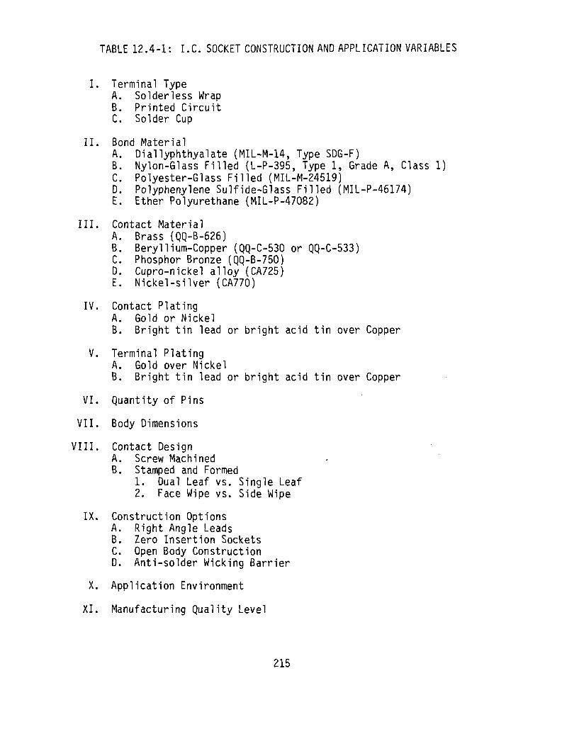
TABLE 12.4-1: I.C. SOCKET CONSTRUCTION AND APPLICATION VARIABLES
Terminal Type A. Solderless Wrap B. Printed Circuit C. Solder Cup
Bond Material A. Diallyphthyalate (MIL-M-14, Type SDG-F) B. Nylon-Glass Filled (L-P-395, Type 1, Grade A, Class 1) C. Polyester-Glass Filled (MIL-M-24519) D. Polyphenylene Sulfide-Glass Filled (MIL-P-46174) E. Ether Polyurethane (MIL-P-47082)
Contact Material A. Brass (QQ-B-626) B. Beryllium-Copper (QQ-C-530 or QQ-C-533) C. Phosphor Bronze (QQ-B-750) D. Cupro-nickel alloy (CA725) E. Nickel-silver (CA770)
Contact Plating A. Gold or Nickel B. Bright tin lead or bright acid tin over Copper
Terminal Plating A. Gold over Nickel
B. Bright tin lead or bright acid tin over Copper
Quantity of Pins
Body Dimensions
Contact Design A. Screw Machined B. Stamped and Formed
1. Dual Leaf vs. Single Leaf 2. Face Wipe vs. Side Wipe
Construction Options A. Right Angle Leads B. Zero Insertion Sockets C. Open Body Construction
D. Anti-solder Wicking Barrier
Application Environment
Manufacturing Quality Level
215

TABLE 1 2 . 4 - 2 : I . C . SOCKET FAILURE RATE DATA
ENTRY NO.
10
n
12
13
14
15
QUALITY
Commercial
Commercial
Commercial
Commercial
Commercial
Commercial
MIL-SPEC
Commercial
Commercial
Commercial
Commercial
Commercial
Commercial
Commercial
Commercial
CONTACT MATERIAL
Phosphor Bronze
Phosphor Bronze
Phosphor Bronze
Phosphor Bronze
Phospnor Bronze
Phospnor Bronze
Beryllium Copper
(1)
Beryllium Copper
Beryllium Capper
Beryl 1 ium Copper
3eryll ium Cooper
3eryllium Copper
Beryl 1ium Copper
3eryllium Copper
CONTACT PLATING
Gold over Nickel
Gold over Nickel
Gold over Nickel
Gold over Nickel
Gold over Nickel
Tin over Copper
Gold over Nickel
(1)
Gold over Nickel
Gold over Nickel
Gold over Nickel
Gold over Nickel
Gold over Nickel
Gold over Nickel
Gold over Nickel
TERMINAL TYPE
Solderless Wrap
Solderless Wrap
Solderless Wrap
Solderless Wrap
Solderless Wrap
Printed Circui t
Printed Circuit
(1)
Solderless Wrap
Printed Circuit
Printed Circuit
Solderless Wrap
Solderless Wrap
Solderless Wrap
Printed Circuit
PINS/ SOCKET
24
16
16
14
14
16
16
16
16
14
16
14
24
28
10
ENVIRONMENT
GF
GF
GF
GF
GF
GF
NS
GF
GF
GF
GF
GF
GF
GF
GF
EQUIPMENT
AN/GYQ-18
AN/GYQ-18
AN/GYQ-18
AN/GYQ-18
AN/GYQ-18
Computer
AN/SLQ-31
point of sales
AN/GYQ-18
AN/GYQ-13
AN/GYQ-18
AN/GYQ-18
AN/GYQ-18
AN/GYQ-18
AN/GYQ-18
FAILURES
i
0
0
0
0
1
0
• 0
0
0
0
0
0
0
PART HOURS
2,135,000
469,791,000
469,791,000
1,156,326,000
1,207,575,000
112,575,000
7,769,000
20,736,000
3,S65,QOO
1,179,300
355,900
18,507,COO
355, ?:-0
355,900
o 7::,3co
2 3,473,129,030
NOTES:
; i ) Unknown
216

Field failure rate data were collected from only the ground, fixed and
naval, sheltered environments. Therefore it was impossible to derive a
complete series of environmental factors based solely on the data. Based on
theoretical considerations, the environmental factors for lower quality
connectors (Table 5.1.12.1-7 in MIL-HDBK-217D) were applied to I.C. sockets.
This assumption was justified because the I.C. socket contact/I.C. lead
interface is analogous to the interface between the male and female portions
of a connector. The lower quality connector factors were applied because the
I.C. lead is representative of a poor quality male connector due to the rough
I.C. lead edges. The environmental factors for lower quality connectors
range from a value of 1.5 for ground, benign and space, flight environments
to a value of 970 for the cannon, launch environment. It was desirable to
normalize the environmental factors to a value of one for the ground, benign
environment. Table 12.4-3 presents both the existing lower quality
connector environmental factors and the normalized factors to be applied to
I.C. sockets. Additionally it was recommended that the environmental
factors should only be applied to avionic and other high vibration
environments if the socketed device was restrained to prevent "walkout".
The hypothesized I.C. socket failure rate prediction model assumed that
failure rate was proportional to-the number of active contacts raised by a
constant, which was approximately equal to one. Since there was insufficient
data to develop a precise measure of the constant, it was assumed to be equal
to one.
The great majority of the collected field experience data pertains to
commercial quality level parts. One data record (entry number 3 in Table
12.4-2) was for military qualified I.C. sockets but it had zero observed
failures. Therefore, development of a quality factor was not feasible. If
it is assumed that commercial quality parts exhibit a higher observed failure
rate, then a proposed model based on the collected data will predict a
pessimistic failure rate for MIL-SPEC I.C. sockets.
217

TABLE 12.4-3: LOWER QUALITY CONNECTOR AND I.C. SOCKET ENVIRONMENTAL FACTORS
Environment
6B 6F
GM
MP
NSB
NS
NU
NH
NUU
ARW
AIC AIT
AIB
AIA
AIF
AUC AUT
ALIB
AUA
AUF
SF
MFF MFA
USL ML CL
Lower Quality Connector TTE
1.5 4.7
25
17
8.1
11
27
26
28
37
10
10
15 15
20
15
15 20
20
30
1.5 17 24
50 58 970
Lower Quality Connector H E ,
Normalized
1.0 3.1
17
11
5.4
7.3
18
17
19
25
6.7
6.7
10
10
13
10
10
13
13
20
1.0 11 16 33 39 650
The base failure rate for I.C. sockets was hypothesized to be a function
of contact material, contact plating, contact design and I.C. lead plating.
218

Due to the relative scarcity of failure rate data, an average base failure
rate value was applied to all I.C. sockets. This assumption resulted in
reduced accuracy for the proposed failure rate prediction model but was
necessary because of the data deficiencies. The proposed model form is then
given by:
X p = Xb x N x TTE
where
Xp = predicted I.C. socket failure rate
Xb = base failure rate = constant
N = number of active contacts
TTE = assumed environmental factor
To derive a numerical value for base failure rate, all data presented in
Table 12.4-2 were normalized by environment and pin count. Normalized point
estimate failure rates were calculated for each data entry by dividing
observed failures by normalized part hours for data entries with observed
failures and by calculating an upper 60% confidence limit for data entries
without observed failures. These failure rate estimates are presented in
Table 12.4-4. Dividing the summed failures by the summed normalized part
hours resulted in a base failure rate estimate of 0.0000126 failures /106
hours. This potential base failure rate value was rejected for two reasons.
First, the value was lower than any of the individual normalized failure rate
estimates, which does not intuitively make sense. Second, the practice of
merging failure rate data when the majority of data records have zero
observed failures has questionable validity. Therefore a base failure rate
value was calculated by computing the geometric mean of the normalized
failure rate estimates for data entries 1 through 6. Data entries 7 through
15 were not included in the calculation because upper confidence limit
failure rates for data records without observed failures are only meaningful
if the failure rate estimate is relatively low. This was not the case for
219

data entries 7 through 15. The geometric mean of the normalized failure
rates for data entries 1 through 6 is:
Xb = 0.0000905 failures/106 hours.
TABEL 12.4-4: I.C. SOCKET NORMALIZED FAILURE RATES
ry No.
1 2 3 4 5 6 7 8 9 10 11 12 13 14 15
Normalized Failure Rate (f/106 hours)
0.00630 0.0000392 0.0000392 0.0000182 0.0000174 0.000179 0.00101 0.000889 0.00185 0.0179 0.0518 0.00114 0.0345 0.0296 0.0414
Number of Observed Failures
1 0 0 0 0 1 0 0 0 0 0 0 0 0 0
Inclusion of this numerical value into the proposed failure rate
prediction model finalized the model development procedure for I.C. sockets.
The proposed model offers the reliability analyst a method to assess the
reliability of I.C. sockets. Currently, MIL-HDBK-217D does not consider
I.C. sockets and the proposed model fills this void.
It should be noted that the proposed failure rate prediction model
applies to I.C. socket failures observed at the socket housing and the
socket/I.C. lead interface. The failure rate contribution of the I.C. socket
terminal is accounted for by the interconnection assembly failure rate
prediction model presented and developed in Reference 1.
220

12.5 References and Bibliography
References
1. Coit, David W., (I IT Research Institute), Printed Wiring Assembly and Interconnection Reliability, Final Technical Report, RADC-TR-81-318, November, 1981.
Bibliography
Augat Inc., Report of Test on 200 Series Low Profile DIP Socket with Beryllium Copper Contact, Test Report No. 178, December, 1979.
Augat Inc., Report of Test on 300 Series Low Profile DIP Sockets, Test Report No. 174, November, 1974.
Augat Inc., Report of Test on 500 Series Dual-In-Line Sockets, Test Report No. 173, February, 1973.
Bryant, N., D Hershberger and J. Coakley, Printed Circuit Board Assemblies from Countermeasures Set AN/ALQ-126; Failure Analysis of, Materials Test Report No. 67-77, August, 1977.
Burndy Electronic Products Laboratory, Test of DILB-P-108 Per MIL-S-83734A (USAF), Formal Report F7608-762, June, 1976.
Coit, David W., (IIT Research Institute), Printed Wiring Assembly and Interconnection Reliability, Final Technical Report, RADC-TR-81-318, November, 1981.
Erickson, J., W. Townes and 0. Leary, R & M of Socketed I.C.'s, IEEE Transactions on Reliability, Vol. R-28, No. 5, December, 1979.
Erickson, 0. and W. Townes, A Study of Integrated Circuit Mounting Techniques for Improved Reliability and Maintainability of FAA Airway Facility Systems, Report No. DELET-TR-79-7, March, 1979.
Gaynes Testing Laboratories, Qualification Testing of Socket, Plug-In, Part No. M83734/10, Order No. 9928-1215, January, 1978.
Howell, D., Socket or Solder, Electronic Products, Vol. 21, No. 1, June, 1978.
Robinson Nugent, Inc., Test Report on DIL I.C. Sockets for P.C.B. Applications, Report No. ICN-375, December, 1974.
221
13.0 THUMBWHEEL SWITCHES
13.1 Device Description
The switches which were considered in this study effort are thumbwheel,
pushbutton and inline rotary switch types as specified by MIL-S-22710. The
generic term "thumbwheel switch" was used as a notation to describe all three
switch types. This term was selected for several reasons. First, thumbwheel
switches are the most widely used of the three rotary switch types. Second,
the pushbutton version of the MIL-S-22710 switch is physically similar to
thumbwheel switches. Only the method of actuation is different. Third, the
inline version of this switch type is rarely used. Although the term
"thumbwheel switch" is used as a convenient notation in this discussion, the
proposed failure rate prediction model applies to all three types of MIL-S-
22710 rotary switches.
Thumbwheel switches typically consist of a thumbwheel with legend, a
housing, a printed circuit board, contacts, a detent spring and eyelets.
Generally there are two styles available. One version has a rotating printed
circuit code disc and fixed contacts while the other version has rotating
contacts and a fixed printed circuit board. In both versions ttie switch can
operate in either direction. The switch position may be set in a variety of
ways including use of a thumbwheel, lever, pushbutton or paddle lever.
Detent action for the switch is provided by a plastic or metal spring, ball
and spring combination, or an integral flexing member which is part of the
spring housing.
Thumbwheel switches are typically designed with 2, 8, 10, 12, or 16
positions and are rated for operating temperatures ranging from -65°C to
125°C. Military versions of the switch are generally designed to meet
military standards for thermal shock, vibration, explosion, salt spray,
moisture, humidity and altitude.
Self extinguishing nylon and molded poylcarbonate are common materials
used in the construction of the switch housing. Contacts are usually made of
222
beryllium copper with gold-over-nickel plating, which offers low contact
resistance and long life. Epoxy glass printed circuit boards are standard.
A wide selection of thumbwheel switch models and options are available.
Thumbwheel switch widths can range from 0.235" to 0.65". Overall switch
height can range from 0.63" to 2.1" and depth behind the panel varies from
0.748" to 2.1". Standard indicator wheel markings include 0 to 7, 0 to 9 and
0 to 15. Character heights usually range from 0.09" to 0.25".
Thumbwheel switches are used wherever a man to digital device interface
is required. By simply "dialing in" the required data on a multipole
thumbwheel, an operator can program a wide variety of functions. The most
common of these is to set operating limits. In some cases, operating the
thumbwheel switch simply changes the configuration of an OR or AND gate
matrix. In others applications, the thumbwheel switch is used to apply
voltage to the appropriate pins of a microprocessor circuit. Depending on
the device being controlled, the thumbwheel switch may be used to stop a
process after a preset number of events has occurred, or at a predetermined
voltage level.
Thumbwheel switches are also used to manually select channels in
multichannel process controllers and data acquisition systems. With a
thumbwheel switch, an operator can manually select a specific stc, in a
lengthy program where an input terminal is not normally available.
Digital control of frequency synthesizers is another area for which the
use of thumbwheel switches is well-suited. Such applications range from test
equipment to radio transmitters. Thumbwheel switches are also used for the
digital control of operations where a display of the preset instruction is
required.
223

13.2 Failure Modes and Mechanisms
The failure modes and mechanisms of thumbwheel switches are similar to
those of other rotary switch types. The expected failure modes include opens
and shorts of the printed circuit board, jitter due to detent wear, and
mechanical wearout problems. A more detailed discussion of rotary switch
failure modes and mechanisms is given in Reference 1.
Contact life is a primary concern for all rotary switches. Several
factors influence the integrity of the interface between the contacts and the
printed circuit board code disc. All metal surfaces are susceptible to the
formation of surface films. Airborne contaminants such as sulfides can
condense on the contact surfaces and thus cause alternations of the physical
and chemical properties of the contact plating material. When a surface film
is softer than the contact material, the contact pressure will squeeze the
film aside. However, when the film is harder than the contact material,
there is a reduction of contact area and an increase in contact resistance.
Brittle films will tend to be fractured away to expose the base metal during
contact mating. Contact materials such as silver, platimum, palladium,
tungsten, molybdenum and nickel are susceptible to the formation of oxide
films. To make electrical contact through the tough and resistive oxide
surface film requires relatively large contact forces. When high
reliability is essential, gold plated contacts are recommended because they
are virtually free from the formation of oxides.
13.3 Thumbwheel Switch Failure Rate Prediction Model
This section presents the proposed failure rate prediction model for
thumbwheel switches. The proposed model is:
Xp = ( X l + N \ 2 ) TTE7rCyC7rL
where
224
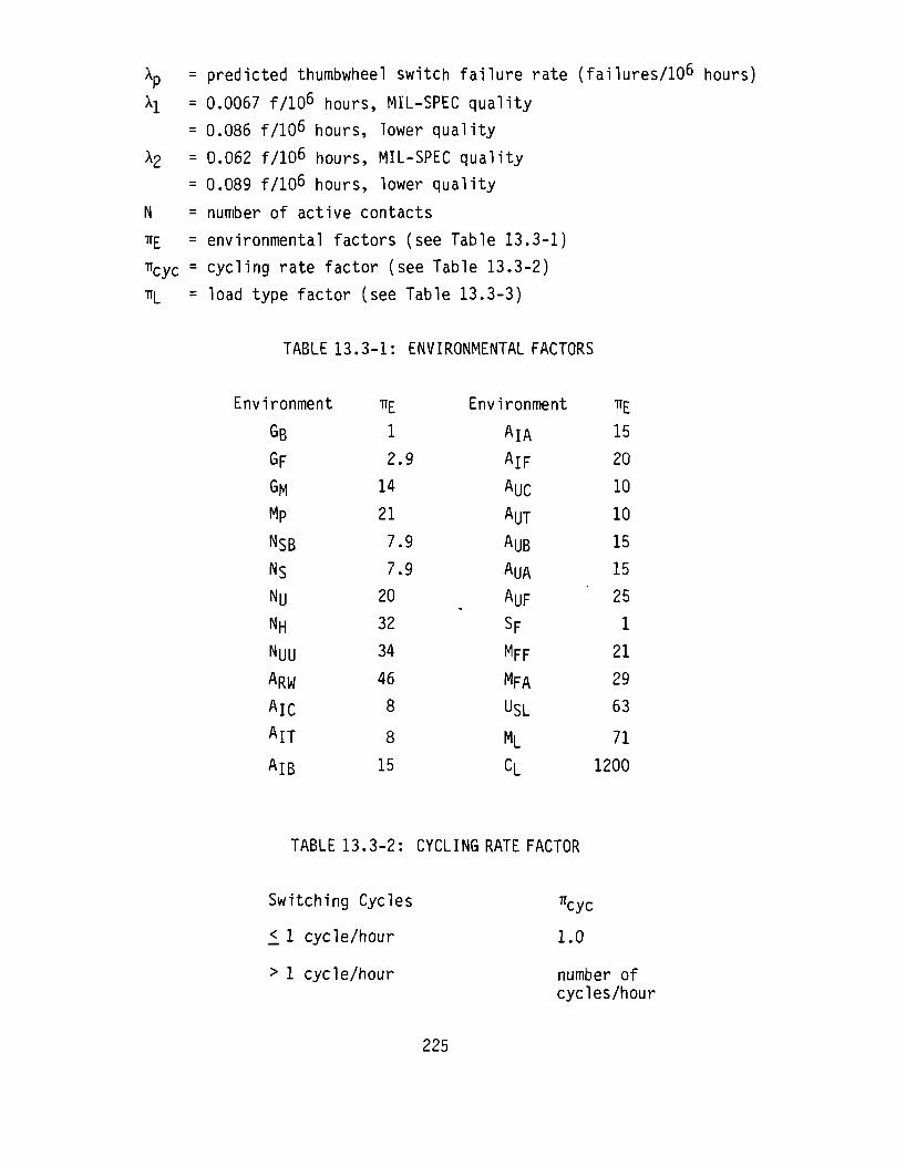
Xp = predicted thumbwheel switch failure rate (failures/106 hours)
\\ = 0.0067 f/106 hours, MIL-SPEC quality
= 0.086 f/106 hours, lower quality
X2 = 0.062 f/106 hours, MIL-SPEC quality
= 0.089 f/106 hours, lower quality
N = number of active contacts
TTE = environmental factors (see Table 13.3-1)
^cyc = cycling rate factor (see Table 13.3-2)
TT|_ = load type factor (see Table 13.3-3)
TABLE 13.3-1: ENVIRONMENTAL FACTORS
Environment
GB GF
GM Mp
NSB NS
Nu NH
NUU
ARW
AlC AIT
AlB
irE
1
2.9 14
21
7.9
7.9 20
32
34
46
8
8
15
Environment
AlA
AlF AUC
AUT
AUB
AUA AUF SF M F F
MFA
USL
ML
CL
TTE
15
20
10
10
15 15
25
1
21
29
63
71
1200
TABLE 13.3-2: CYCLING RATE FACTOR
Switching Cycles % y C
<. 1 cycle/hour 1.0
> 1 cycle/hour number of cycles/hour
225

TABLE 13.3-3: LOAD TYPE FACTOR
Stress
S
0.05
0.1 0.2
0.3
0.4
0.5 0.6
0.7 0.8
0.9
1.0
Resistive
1.00
1.02
1.06
1.15
1.28
1.48
1.76
2.15
2.72
3.55
4.77
Load Type
Inductive
1.02
1.06
1.28
1.76
2.72
4.77
9.49
21.4
where
s _ operating load current rated resistive load
2 _ (S/ .8) f o r r e s i s t i v e . IiL - e
2 = e(
s/-4) f° r inductive.
e(S/.2)2 for lamp.
CAUTION: This model applies to the switching function only. The model does not consider the contribution of any discrete components (e.g., resistors, diodes, lamp) which may be mounted on the switch. The failure rate of these devices must be calculated using the appropriate section in MIL-HDBK-217 and added to the failure rate of the switch.
This model applies to a single switch section. This type of switch is frequently ganged to provide the required function. The model must be applied to each section individually.
Lamp
1.06
1.28
2.72
9.49
54.6
226
13.4 Failure Rate Model Development
The initial approach utilized for failure rate model development of
thumbwheel switches was to identify and quantify significant failure rate
model parameters by analysis of field experience data. The field experience
failure rate data which were available are presented in Table 13.4-1.
Application and construction variables were identified for thumbwheel
switches and are presented in Table 13.4-2. The application and construction
variables represent possible failure rate model parameters. The initial
model development approach was unsuccessful due to field experience data
limitations. Alternate model development approaches were explored because
of the failure of the initial approach to yield an acceptable failure rate
prediction model.
The alternate approach which was implemented for model development was
based on analysis of the existing MIL-HDBK-217D failure rate prediction
model for rotary switches (Section 5.1.11, MIL-HDBK-217D). The failure rate
data presented in Table 13.4-1 were analyzed to determine whether the
existing rotary switch model could be applied to thumbwheel switches without
introducing error. Analysis of the the data did not invalidate the
assumption that the existing rotary switch modifying factors based on
cycling rate, load type and environment could be applied to thumbwheel
switches. Therefore the assumption was made that a proposed failure rate
prediction model for thumbwheel switches would be of the following form:
Xp = (Xi + NX2) iTETTcyc L
where
predicted thumbwheel switch failure rate
base failure rate constants (unique values for MIL-SPEC and
commercial quality grades)
number of active contacts
Xp
X1>X2
N
227
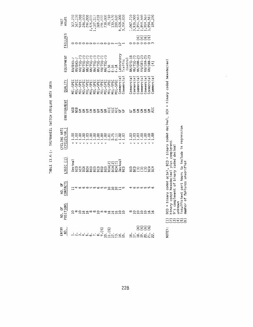
o o o o o o o o o o o o o o o
m r o o o o o o o O O - — < C \ J C \ J O O C \ J C \ J O O O O O O O O < ^ L T ) C 0 O O
o o o o o o o - - i O t D t £ i O U2 O r-^ O Lf) Lf) Lf) Lf) C\J
n n c j i C M C N j C ' - H n c s j r ^ i—« C M «3- C M
r-^ k£) *3" «cr *3" <T CTi U D r o a") L D L D L D CO O CT» CT» CT» CTi CD •—•
O O O O O O O O O O O C M - — i CM •—<
*x) vr; *x) y£>
o o o o o o ro
Cd Cd c CD CO t
<«ai'=r«a:«a:<«a:«a:
i +-> o o i i <or cy fo-r- i-o'O'CCc^ccct: -—«•
i— i— *=c <: ct o v- c o i— o o o c o — -w n n r ) J2 ra o ^ ^ ^ ^ ^ ~ - ^ z :2 i i i m t- o z: z z z: z ^ < < L L I U J L L I _ l h < < < < < <
o -
U O U U U U U U U U U U U * i - ' i -U J L ^ U J U J L ^ L J J L J J L L J L L J L J J L L J L J J L J J U t->
o_ci_ci_c^ci_ci_c^ci_ci_a.ci_ci_a. i- i-
I I I I I I I
u Z u o o u u
mill!
l O O O C D O O O O c t c t c r O C D O O O O O O c t
o o o o o o o o o o - — ' L O ^ H O O
O O O O O O O O O O O C M ^ H O O
o o o o o o o o o o o o o o
v v v v v v v v v v V V V V V
o
u +-> c
> > QJ
s- E to QJ
c •— i - CL
r— A3
1
U
u o o ^ c ^ o o o o o a i i r n : u o ( U U U U U U U U U U U U U O J U
Q m c Q m m m m m m i n i n f n m Q m
O Q - — - — - — m 3= u u n n n u u CD CD — — — - en en
o o > — t ^ T » X ) » X ) » X ) L n L f J t X ) L f J L f J O O O , — ' L O *3 " t£ ) Lf> Lf> Lf> Lf> t£ )
Q ^ QJ U D T D CD >— O
CL U
<—-—>> to to i-+ J p ID
u •<- c o u ••-
QJ J 3 " D " D QJ ( 0 4 -
" D X O O QJ
u j r +-> c
> , T 3 QJ S- QJ E A3 " D QJ C O r -
C " D •f~ QJ
O M -+-> -r~
L-LO QJ S- > 3 C O 3
. C t/1
+-> QJ S- t . m 3 C L i —
-•-> A3 C M -QJ
• . - 4 -
O t D O k D ^ D C O C O O C O C O l D l D l D O O CO O O O O <X> <X>
[] S- U O S - QJ A3 C 3 _Q
O C LO _ * : t / i E O • < - - C C 3 CO - O CTi 3 • < - C
i—i c \ j r o ^ r LTJ \&
VD UD UD CD
228

TABLE 13.4-2: THUMBWHEEL SWITCH CONSTRUCTION AND APPLICATION VARIABLES
I. Type A. Thumbwheel B. Inline
C. Pushbutton
II. Number of Positions
III. Number of Contacts
IV. Logic A. Decimal B. Binary Coded
1. Octal 2. Decimal 3. Hexadecimal
C. Other V. Housing and Thumbwheel Material
A. Polycarbonate B. Self-extinguishing Nylon
VI. Contact Material A. Beryllium Copper B. Other
VII. Contact Plating A. Gold over Nickel B. Tin over Copper
C. Other
VIII. Actuation Frequency (#Actuations per Unit Time)
IX. Application Environment
X. Manufacturing Quality Level
XI. Load Type A. Lamp B. Inductive C. Resistive
XII. Current Level A. Rated Resistive Current B. Actual Current
229

T\£ = environmental factors
" cyc = cycling rate factor
TTL = load type factor
To determine point estimate values for the two base failure rate
constants, the data were separated by quality level and normalized for
environment, cycling rate and load type using the assumed rotary switch
failure rate model modifying factors. Each data entry was for thumbwheel
switches which were switching a resistive load. The ratio of applied current
to rated resistive current was unknown for the majority of data entries. The
assumption was made that the ratio of applied current to rated resistive
current was equal to 0.10 for all data entries. This is a realistic
assumption because thumbwheel switches are used almost exclusively for
switching decimal or binary logic circuits where a low current is required.
Point estimate failure rates were calculated for each data entry by dividing
the number of observed failures by the part hours for data entries with
observed failures, and by calculating an upper 60% confidence limit value for
data entries without observed failures. The normalization function and the
resulting regression model are given by:
*N = Vl^^cyc^L) = M + N X2
where
Xfsj = normalized failure rate
XQ = observed failures/part hours, data entries with observed failures
XQ = upper 60% confidence limit, data entries w/o observed failures
TIE = assumed environmental factors
TTCyC = assumed cycling rate factor
TIL = assumed load type factor
= 1.02, resistive load stress = 0.10
Stepwise multiple linear regression analysis as described in Section 3.1
was applied to the data. The failure rate data had been separated by quality
230

level and therefore two regression analyses were required. The data records
which were entered into the regression analyses are data entries 1-8, 10, 12-
16 and 22 in Table 13.4-1. Data entries which were not included in the
regression analyses either had insuffient part hours to estimate a failure
rate without observed failures or lacked other requisites. The results of
the two regression analyses are:
XH,MIL-SPEC = -0.5197 + 0.1317(N), R2 = 0.60
*N,commercial = °-0860 + 0.0888(N), R2 = 0.30
The regression solution for commercial quality thumbwheel switches is
satisfactory. However, the regression solution for military qualified
thumbwheel switches is illogical, particularly because it predicts a
normalized failure rate which is negative for thumbwheel switches with less
than four contacts. Probable explanations for this result are (1) there was
an inadequate number of data entries with observed failures to accurately
apply regression analysis, and (2) no data entries were available for
thumbwheel switches with less than four contacts. Therefore, the regression
solution for military qualified thubmwheel switches was rejected and an
alternate modeling approach was proposed.
The existing MIL-HDBK-217D equation for MIL-SPEC ceramic RF wafer rotary
switches and MIL-SPEC medium power wafer rotary swtiches is given by:
Ab = 0.0067 + 0.00003(N) failures/106 hours
where
N = number of active contacts
The dominant failure mechanisms associated with thumbwheel switches
pertain to the switch contacts. Therefore the second base failure rate
constant value in the above equation should not be applied to thumbwheel
switches without verification with empirical data. However, it was assumed
231

that the first base failure rate constant could be applied to all types of
rotary switches including thumbwheel switches. Therefore the failure rate
equation for thumbwheel switches was assumed to be of the form:
Xb = 0.0067 + X 2 W failures/106 hours
The failure rate data for MIL-SPEC thumbwheel switches was then analyzed to
determine the remaining unknown base failure rate constant. The solution of
a regression analysis which is forced through the origin and has only one
independent variable, is given by:
Y = biXi
bl = £Ul,iYi)/i:(Xi5i)2
where
bi = regression coefficient
Y = dependent variable X-L = independent variable.
An additional variable was defined so the equation for MIL-SPEC base failure
rate would be of this form. The additional dependent variable is defined as
follows:
XR = XN " 0.0067
where
XR = additional regression dependent variable
X|\j = observed failure rate normalized for environment, cycling rate
and load type.
232

The regression analysis model form was then modified to:
XR = XN - 0.0067 = X2(N)
and the second base failure rate constant (X2) for MIL-SPEC thumbwheel
switches was derived by:
X2 = E(XRN)/£N
= 34.279/556 = 0.0617.
The complete base failure equation for MIL-SPEC thumbwheel switches was as
follows:
Xb = 0.0067 + 0.062(N).
Derivation of the second base failure rate constant for MIL-SPEC
thumbwheel switches completed the model development process. The proposed
model presented in its complete form including the assumed modifying factors
for environment, cycling rate and load type was included in Section 13.3.
Thumbwheel switches are available -with character illumination
capabilities, or with diodes or resisters mounted on the external printed
circuit board. The proposed failure rate prediction model for thumbwheel
switches does not account for these additional components. The appropriate
sections of MIL-HDBK-217D must be used in conjunction with the proposed
thumbwheel switch failure rate prediction model for these hybrid types of
thumbwheel switches.
13.5 References and Bibliography
References
1. Guth, G.F., Development of Nonelectronic Part Cyclic Failure Rates, Final Technical Report, RADC-TR-77-417, December, 1977.
233
Bibliography
Arno, R.G., Nonelectronic Parts Reliability Data, NPRD-2, Summer 1981.
Guth, G.F., Development of Nonelectronic Part Cyclic Failure Rates, Final Technical Report, RADC-TR-77-417, December, 1977.
Henriksen, D., Thumbwheel Switches, Electronic Products, July 1, 1979.
Pogmore, J., Selecting Switches for Harsh Environments, Electronic Products, June, 1982.
234

14.0 METERS
14.1 Part Description
The meters considered in this study are all ultimately either AC or DC
electromagnetic current measuring devices.
DC meters utilize a core magnet and moving coil movement (D'Arsonval
movement). DC meters are based on the principle that a current carrying
conductor in a magnetic field will experience a force. If a conductor in the
uniform magnetic field is constrained by a linear spring, the motion against
the spring will be proportional to the current in the conductor. In this
movement, a permanent magnet is enclosed by the moving coil and the return
path of the flux is through the coil to an iron ring surrounding the coil.
This type of movement is self shielding and is little affected by magnetic
panels or stray magnetic fields. By using precision resistors, either
internal or external to the meter, deflection can be made proportional to
voltage.
AC meters including Radio Frequency meters normally use iron vane
movements. This movement is designed around the fact that a piece of ferrous
metal placed inside a coil is magnetized. When two pieces of metal (or
vanes) are inside the same coil, they are identically magnetized and repel
each other. By making one vane solid and pivoting the other, the movement
responds to the rms value of current or voltage. By using rectifiers to
produce positive average voltage, the core magnet movement is often used to
give an rms reading of sinusoidal voltages.
Meters are categorized by function which includes:
o Primary Function
Ammeter
Voltmeter
Other
235

o Application
- AC
- DC
The 'Other' application may be oil pressure, temperature, decibel, %
load, VSWR gauge, etc. The most widely used AC meters are 60Hz for ground
fixed, naval and ground mobile applications and 400Hz for airborne
applications. Higher frequency meters up to 50KHz are available. A
voltmeter, as the name indicates, is a voltage measuring instrument. This
device is actually current sensitive, but by use of proper internal (or
external) resistance is made to give a correct voltage indication. Meter
movements are characterized by the amount of current required to deflect the
pointer full scale (e.g. 50ua or 1 ma) and/or by the series resistance of the
movement. Meters are characterized by their function, accuracy and input
impedance. Input impedance is particular!'ly important for voltage meters
since it has a direct affect on the accuracy of the voltage reading. In most
applications, ammeters use shunt resistors across the meter movement to
accomodate higher current levels.
Meters are used as visual panel indicators on most military equipments.
14.2 Failure Modes and Mechanisms
The failure modes of meters are:
o Degradated operation
spring relaxation
resistance drift in shunt or series resistances
shorted coil winding (partial)
leaky rectifier diode
balance weight shift
o Catastrophic failure
bearing wear or dirty bearing
open coil winding
236
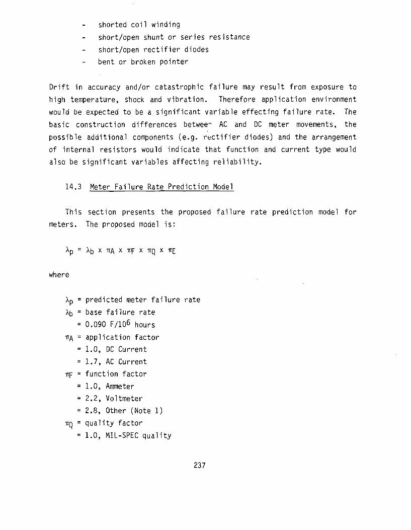
shorted coil winding
short/open shunt or series resistance
short/open rectifier diodes
bent or broken pointer
Drift in accuracy and/or catastrophic failure may result from exposure to
high temperature, shock and vibration. Therefore application environment
would be expected to be a significant variable effecting failure rate. The
basic construction differences between AC and DC meter movements, the
possible additional components (e.g. rectifier diodes) and the arrangement
of internal resistors would indicate that function and current type would
also be significant variables affecting reliability.
14.3 Meter Failure Rate Prediction Model
This section presents the proposed failure rate prediction model for
meters. The proposed model is:
X p = X b X 7TA X 7TF X 7TQ X TT^
where
Xp = predicted meter failure rate
Xb = base failure rate
= 0.090 F/106 hours
TT/\ = application factor
= 1.0, DC Current
= 1.7, AC Current
TTF = function factor
= 1.0, Ammeter
= 2.2, Voltmeter
= 2.8, Other (Note 1)
TTQ = quality factor
= 1.0, MIL-SPEC quality
237

= 3.4, lower quality
ff£ = environmental factor (see Table 14.3-1)
Notes: (1) Includes meters whose basic meter movement construction is an
ammeter but which contains internal conversion elements not
normally found in an ammeter.
TABLE 14.3-1: ENVIRONMENTAL FACTOR
Environment
GB
GF
GM Mp
NSB
Ns Nu NH Nyu
ARW
AlC AIT
AlB
*E 1.0
3.8 24
26
11
14
36
41
29
60
21
42
21
Environment
AlA
AlF AUC AUT
AUB
AUA
AUF
SF MFF
MFA
USL ML
CL
*E 42
42
50
73
50
73
73
2.
13
N/A N/A
94
N/A
14.4 Failure Rate Model Development
The approach used for model development was to identify significant
parameters by analysis of the meter field experience data. The model
parameters were then quantified using the same data. The results were given
a thorough analysis to determine if they were consistent with theory at the
conclusion of each step. The meter failure experience data collected in
support of this study are presented in Table 14.4-1.
238

—1 C 3 we < > en
C\J * r -cr C\J ro ro t—i O
• • > .
LD O l Cn C\J C\J ro -cr co
c o c o » — i c O t — i c i i n i n i n
^ • C O O O J O O f l - M ^ ID O CTi LT) CTi P-* ID
C\J f—I C\J C\J
ID O CO ^
en ro
r O r H t O r H
O H S N en I D • - I CO
ro r-» en * r I D o
C\J r>- C\J t—1 «—1
c )
** o •—i
m O ro c\j r H t H O O C M
• • • >
.—I C\J .—1 C\J
.—1 C\J o o r>- en
ro I D .—I I D
I—
O CL
s? I
L i -
S— S ^ S— S— S—
o o o o o 4-) 4-> 4-> 4-> 4-> ID IO IO IO IO S_ S^ S_ 1 - S-OJ QJ QJ OJ QJ C C C C C
QJ QJ QJ QJ QJ
o o o o o
o C U D O-CVJ 3 I
CO CO cr
. ^ CO <E <E <E <E 5 ^ r o r o r o r o ro "Z. U J U J U J U J K
P-^ I D C\J i-\ r-\ r-\
S - S - S - S - S - S -
o o o o o o 4_) 4-> 4-> 4-> 4-> 4-> ro ro ro ro ro ro S— S ^ 1 — 1 — S— S— OJ QJ QJ QJ OJ OJ C C C C C C
^ o ^ o a j Q j a j a j Q j Q j i c \ j c \ j e > o e > e > e > o i i i
C O C O Q j a j a j Q j Q J Q J
crcr-—-—-—-—•—•— CO CO •— -.- •.- •.- -.- -.-^ . ^ . . 0 . 0 . 0 . 0 . 0 . 0 z z o o o o o o <t<t2:2:s:s:s:s:
00>-f">r- . .—i.—1«—if-^^-^-^r^-o^ooo^ 'OO*—<•—ir-*«—1«—1«—i O O ^ D ( N H D « 3 1 D M C J i O > C n O i O C O O r O l I 3 ^ D ^ D ( \ H D 1 0 U 3 o o H « j a i o i o i q ' < j ^ ' q - < j o i £ i o o o o c n o i ^ ' O i a i ^
o r -» r -»*3-u3U3*r>*3-c \ j c \ j c \ j c \ Jo r - . oo»—i i ro iD^T^ iDiD r-» r-» ^ - oo
C \ j r O H H r H r O « * O C M O H O r H H l D M O O C M l f ) H O H r H i—I C\J C\J f—I «—I
CD O O O O 3 3
2:02:2:2:2:2:2:2:2:2:2:2:2:2:2:2:2:2:2:2:2:2:2:
u_ *— < < < > < < > > < < > > < < < < < Z L I - V : L I - I ~ " - < ' - '
4-> QJ S- •<-QJ 4-> QJ O E QJ •*->
E QJ 4-> £ -• M > > I -
ro u +J o
QJ ro ro QJ 3 3 U v) c r o •<-
-*- OJ <— TJ o i - 1 - c
2 = L L . _tf —> If I I II II II II II
« t < > 2 = L L . i £ -
4-> QJ ro i_ + J C QJ QJ i - •*-> E QJ QJ 4->
<— E O
f-H .—I . - I f — l f — I , — I . — I . — I . — I . — I C V J C \ J C \ J C \ J C V J
239

Application and construction variables were identified for meters (Table
14.4-2). The application and construction variables represent factors which
were determined whenever possible for all collected data.
TABLE 14.4-2: METER CONSTRUCTION AND APPLICATION VARIABLES
I• Type A. Ammeter B. Voltmeter C. Special Meter D. Other
II. Enclosure Type A. Nonwater Tight B. Water Tight
III. Application A. dc
B. ac
IV. Environment
V. Manufacturing Quality Level
Stepwise multiple linear regression analysis as described in Section 3.1
was applied to the meter failure experience data. All functions other than
ammeter and voltmeter were grouped under the heading 'other'. The first
iteration of the regression program disclosed that the unknown applications
(source 1, 13, 15, 16) had a significant impact on the results. The data
sources with the unknown application factors were deleted since they had a
significant impact on the regression, and a second regression was run. This
second regression resulted in the following failure rate prediction model:
where
^p = meter failure rate in failures/10^ hours
^b = base failure rate
240

= 2.1687 F/106 hours
Tip = funct ion fac to r
TTQ = qua l i t y fac to r
ff[r = environment fac to r
The details of the regression are given in Table 14.4-3.
TABLE 14.4-3: RESULTS OF METER REGRESSION ANALYSIS
Variable Coefficient Standard F-Ratio (bi) Error
Ammeter Voltmeter Other MIL-SPEC Quality Lower quality G^ environment N$B environment N$ environment AJC environment AfM environment *b
1.0 0.8089 (1) 1.0327 (1) 1.0 1.2202 (1) 1.0 0.6702 (1) -0.3573 (1) 1.2233 (1) 3.8502 (1) 2.1687 (1)
--
0.7232 0.6662
—
1.3220 —
1.3220 0.8064 0.7534 1.0057
—
—
1.25 2.40 --
0.85 --
0.26 0.20 2.64
14.66 —
Degrees of freedom = 16
Notes: (1) factor = exp(bi)
The variables voltmeter, other, AJC and AR^ were significant at a 70%
confidence level. The variable for quality level was significant at a 60%
confidence level. The environment variables N$B and N$ were forced-in by
assigning a 0% confidence level. These variables were forced into the model
by specifying a zero critical f ratio since they would be required to
generate estimates for the entire range of environments. The standard error
statistic allows for the calculation of confidence intervals for the
variables. Table 14.4-4 lists the point estimate, lower 20% confidence bound
and upper 80% confidence bound for the variables.
241
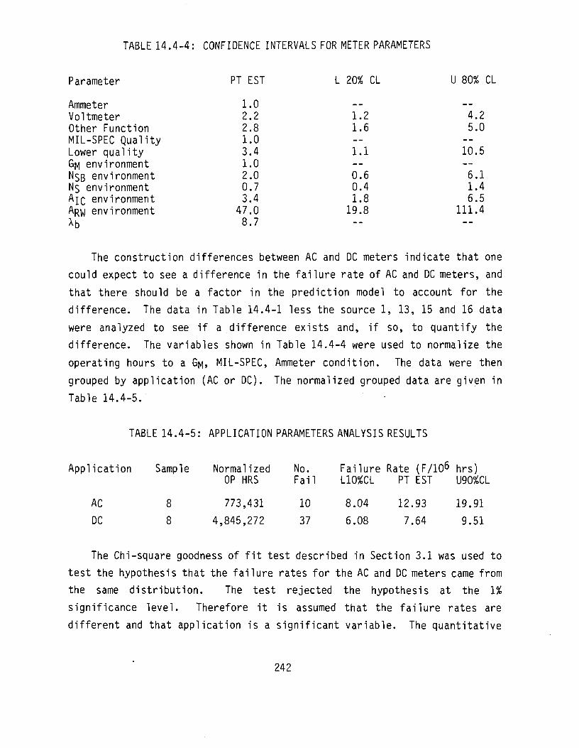
TABLE 14.4-4: CONFIDENCE INTERVALS FOR METER PARAMETERS
Parameter
Ammeter Voltmeter Other Function MIL-SPEC Quality Lower quality GM environment Nsg environment Ns environment AJQ environment ARM environment Xb
PT EST
1.0 2.2 2.8 1.0 3.4 1.0 2.0 0.7 3.4
47.0 8.7
L 20% CL
1.2 1.6 —
1.1 —
0.6 0.4 1.8
19.8 —
U 80%
--
4.2 5.0
—
10.5 —
6.1 1.4 6.5
111.4 —
The construction differences between AC and DC meters indicate that one
could expect to see a difference in the failure rate of AC and DC meters, and
that there should be a factor in the prediction model to account for the
difference. The data in Table 14.4-1 less the source 1, 13, 15 and 16 data
were analyzed to see if a difference exists and, if so, to quantify the
difference. The variables shown in Table 14.4-4 were used to normalize the
operating hours to a G^, MIL-SPEC, Ammeter condition. The data were then
grouped by application (AC or DC). The normalized grouped data are given in
Table 14.4-5.
TABLE 14.4-5: APPLICATION PARAMETERS ANALYSIS RESULTS
Application Sample Normalized No. Failure Rate (F/10^ hrs) OP HRS Fail L10%CL PT EST U90%CL
AC 8 773,431 10 8.04 12.93 19.91
DC 8 4,845,272 37 6.08 7.64 9.51
The Chi-square goodness of fit test described in Section 3.1 was used to
test the hypothesis that the failure rates for the AC and DC meters came from
the same distribution. The test rejected the hypothesis at the 1%
significance level. Therefore it is assumed that the failure rates are
different and that application is a significant variable. The quantitative
242

difference was calculated by taking the ratio of the normalized observed
failure rates. The results of this calculation are:
Application ^j\
DC 1.0 AC 1.7
The failure rate prediction model was then revised to include this factor.
The revised model is:
Xp = xb x A x ^ F x * Q x ^ E
where
Xp = Xb ^F ^Q ^E were defined previously 71/\ = application factor
Only three of the environments (AJQ, GM, ARW) were identified as
significant variables in the regression analysis. This does not imply,
however, that environment is not a significant factor affecting reliability.
Theoretically, environmental stress has a large effect on reliability and
therefore an approach was developed to derive parameters for the remaining
environments defined in reference 1. The approach used to develop the
environmental factors was to apply regression techniques to the data and the
environmental severity ratios presented in reference 2, Figure 2.3-1. These
severity ratios are presented in Table 14.4-7. Two regressions were run.
The first assumed a model of the form:
"E, obs = A Sn
where
71E, obs = observed environmental factors for AJQ, G^ and AR^
S = environmental severity ratios
243
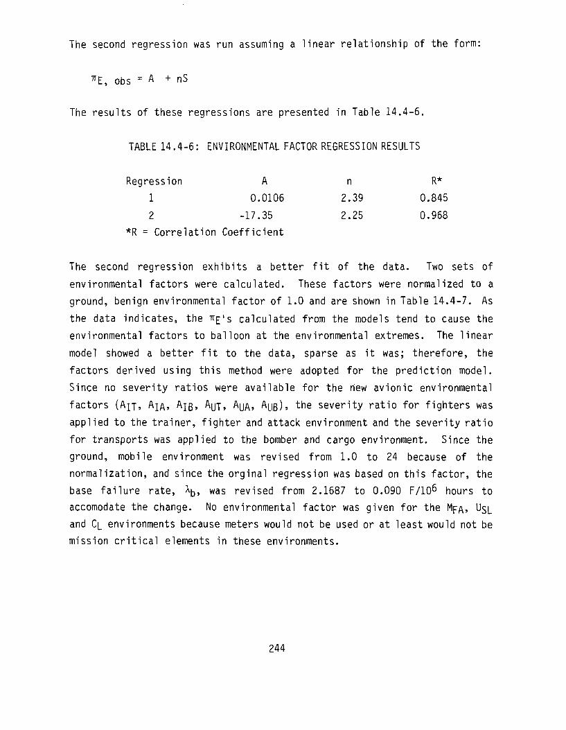
The second regression was run assuming a linear relationship of the form:
^E, obs = A + nS
The results of these regressions are presented in Table 14.4-6.
TABLE 14.4-6: ENVIRONMENTAL FACTOR REGRESSION RESULTS
Regression A n R*
1 0.0106 2.39 0.845
2 -17.35 2.25 0.968
*R = Correlation Coefficient
The second regression exhibits a better fit of the data. Two sets of
environmental factors were calculated. These factors were normalized to a
ground, benign environmental factor of 1.0 and are shown in Table 14.4-7. As
the data indicates, the TT^'S calculated from the models tend to cause the
environmental factors to balloon at the environmental extremes. The linear
model showed a better fit to the data, sparse as it was; therefore, the
factors derived using this method were adopted for the prediction model.
Since no severity ratios were available for the new avionic environmental
factors (AIT, AI/\, Ajg, Ayj, A(JA, AJJB)> the severity ratio for fighters was
applied to the trainer, fighter and attack environment and the severity ratio
for transports was applied to the bomber and cargo environment. Since the
ground, mobile environment was revised from 1.0 to 24 because of the
normalization, and since the orginal regression was based on this factor, the
base failure rate, ^, was revised from 2.1687 to 0.090 F/106 hours to
accomodate the change. No environmental factor was given for the MpA, U$|_
and C|_ environments because meters would not be used or at least would not be
mission critical elements in these environments.
244
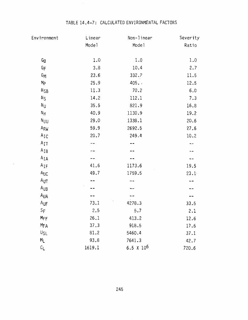
TABLE 14.4-7: CALCULATED ENVIRONMENTAL FACTORS
Environment Linear Non-linear Severity
Model Model Ratio
GB
SF
GM Mp
NSB NS Ny
NH NUU
ARW
AlC AIT
AlB
AlA
AlF
AUC AUT
AUB AUA
AUF
sF MFF MFA
USL ML
CL
1.0 3.8
23.6
25.9
11.3
14.2
35.5
40.9
29.0
59.9
20.7
—
—
—
41.6
49.7
—
—
—
73.1
2.5
26.1
37.3
81.2
93.8
1619.1
1.0 10.4
332.2
405. .-
70.2
112.1
821.9
1130.9
1338.1
2692.5
249.4
—
—
--
1173.6
1759.5
—
—
—
4278.3
5.7
413.2
918.5
5460.4
7641.3
6.5 X 10 6
1.0 2.7
11.5
12.5
6.0
7.3
16.8
19.2
20.6
27.6
10.2
—
—
—
19.5
23.1
—
—
—
33.5
2.1
12.6
17.6
37.1
42.7
720.6
245

14.5 References and Bibliography
References
1. Edwards, E., et.al., Avionic Environmental Factors For MIL-HDBK-217, Final Technical Report, RADC-TR-81-374, January, 1982.
2. Kremp, B.F. and Kimball, E.W., Revision of Environmental Factors For MIL-HDBK-217B, Final Technical Report, RADC-TR-80-299, September, 1980.
Bibliography
Arno, Robert G., Nonelectronic Parts Reliability Data, Reliability Analysis Center Document, NPRD-2, Summer, 1981.
Edwards, E., et.al., Avionic Environmental Factors For MIL-HDBK-217, Final Technical Report, RADC-TR-81-374, January, 1982.
I IT Research Institute, Electronic Reliability Design Handbook, Volume II, Contract Data Item, Contract F30602-78-C-0281, 1981.
Kremp, B.F., and Kimball, E.W., Revision of Environmental Factors For MIL-HDBK-217B, Final Technical Report, RADC-TR-80-299, September, 1980.
MIL-M-10304E, Military Specification, Meters, Electrical Indicating, Panel Type, Ruggedized, General Specification For, May, 1974.
MIL-STD-1279, Meters, Electrical Indicating, Selection and Use of, September, 1970.
QPL-10304-22, Qualified Products List, Products Qualified Under Military Specification MIL-M-10304, Meters, Electrical Indicating, Panel Type, Ruggedized, General Specification For, June, 1980.
246

15.0 FUSES
15.1 Device Description
A fuse is an intentionally weakened part of an electrical or electronic
circuit. Its purpose is to protect the other elements of the circuit from a
possibly damaging overload. Fuses are used to protect many different types
of circuits. In some instances, fuses are used to protect only the wiring
and prevent a fire. In other instances, they are used to protect a \/ery
sensitive meter or an electronic assembly.
Military type fuses are generally a glass-bodied cartridge with nickel-
plated brass caps. High-amperage fuses are made of a punched zinc alloy
element. Low-amperage fuses are constructed with a filament wire which can
be of a variety of materials including copper, platinum and many alloys to
accomplish the desired result.
Fuses are the safety valves of electrical circuits. Therefore, it is
important that they operate or "blow" before damage occurs in either the
equipment or the wiring being protected. Conversely, nuisance blowing is not
desired. Thus, fuses must not blow too easily and cause open circuits when
the equipment is operating normally.
It is obvious that time and current are the controlling factors in the
function of a fuse. There is a time and current relationship at which the
circuit will operate satisfactorily and cause no damage to equipment or
wiring. There is also a time and current relationship at which the equipment
will be damaged. In other words, the time-current characteristics of the
fuse must conform to the time-damage characteristics of the equipment.
There are three basic types of fuses depending on the particular
application. They are, (1) Fast-blowing fuses which are used for instrument
protection where fast action is necessary in order to protect the equipment,
(2) Medium-blowing fuses which are used for general applications and (3)
247

Slow-blowing fuses which are used for applications where a time lag is
desirable.
Fast-acting fuses are designed to carry 100% of current rating and blow
rapidly at very slight percentages of overload. For example, they typically
require milliseconds to operate at high overload currents. The greater the
overload, the more rapidly the circuit opens. There is very little mass in
the filament used and therefore the reaction can take place very quickly
under short-circuit conditions. This filament is generally made of silver,
platinum, or other precious metal alloys. These fuses are manufactured with
wire diameters as low as 0.000020 inches. Obviously this filament will open
the circuit under adverse conditions before any damage can be done in other
parts of the circuit.
Medium time delay fuses are by far the most widely used. These fuses are
designed to protect a non-critical device, wiring, or equipment at minimum
cost. In general, they are designed to carry 110% of rated current for a
minimum of four hours. Circuits will be protected if an overload of 135% of
rated current is applied to the fuse. In this case the fuse will open in less
than one hour. If an overload of 200% of rating is placed on the circuit, the
fuse will open the circuit in a maximum of 30 seconds. The action of these
fuses is not as rapid as the fast-acting fuse. However, they are
satisfactory in the majority of fuse applications.
The slow-blow fuse has a time-lag characteristic. Many circuits or
pieces of equipment have a current in-rush which is normal for the operation
of the equipment. The starting of a motor is an example. Until the motor is
up to speed, the current is far higher than the normal operating current.
This is normal operation for this circuit, so it is not desired that the fuse
open the circuit during these conditions. Therefore, a fuse must be designed
with sufficient mass or time lag to prevent nuisance blowing. In some highly
inductive or capacitive electronic circuits, this same characteristic is
required.
248

15.2 Failure Modes and Mechanisms
Fuses have two principal failure modes: open, and failure to open. Any
premature interruption of the current flow such as a mechanical breaking of
the fuse element would be classified as an open. A failure to open is when
current flow levels exceed the fuse rating and the fuse element does not open
the circuit. Failure to open is most commonly caused by electrically
conductive material shorting the fuse terminals together. Even a ^ery small
increase in resistance due to corrosion, loose connections, poor mating of
contact surfaces or loss of tension in the fuse holder clips can generate
sufficient heat to cause fuse functioning without a change in circuit
current.
Fuse and fuseholder parts are generally required to have a high copper
content and therefore are subject to rapid corrosion in contaminated
environments. This corrosion is usually in the form of nonconducting oxides.
Plated fuse parts offer initial protection from corrosive environments, but
will tarnish with time.
Fuses of the glass and ceramic types have been found to be resistive to
high and low temperature, thermal shock, sand and dust, "humidity, vibration
and mechanical shock. The smaller the fuse in physical size, the more
resistant it is to shock and vibration. Small dimension fuses resist shock
tests well. There have been no reports of failure of any kind under the
usual shock tests of 15G and 30G with an 11 millisecond duration. The reason
that the relatively smaller fuses are resistant to shock and/or vibration
stresses is that the fuse filament is short and does not easily resonate.
15.3 Fuse Failure Rate Prediction Model
This section presents the proposed failure rate prediction model for
fuses. The proposed model is:
Xp = Xb x TTE
249

where
Xp = predicted fuse failure rate (failures/106 hours)
Xb = base failure rate
Xb = 0.010 failures/106 hours
TT£ = environmental factor (see Table 15.3-1)
TABLE 15.3-1: ENVIRONMENTAL FACTORS
Environment
GB
GF
GM
Mp
NSB Ns
Nu NH NUU
ARW
AlC
AIT
AlB
E 1.0
2.3
7.5 8.1
4.4
5.2
10 12
12
16
6.8
12
6.8
Environment
AlA
AlF
AUC Ayr
AUB
AUA
AUF
SF M F F
MFA
USL
ML
cL
*E 12
12
13 18
13
18
18
1
8
11
20
22
230
15.4 Failure Rate Model Development
The reliability modeling of fuses presents a unique problem. Unlike most
other electrical and electromechanical parts, there is very little
correlation between the number of fuse replacements and fuse failures.
Generally when a fuse opens or "blows" something else in the circuit has
created a current overload condition and the fuse is simply functioning as
designed. Additionally, categorizing fuse field replacements as either fuse
failures or fuse "functions" is very difficult. Isolated fuse replacements
which would appear to be a failure may have been caused by a transient
250

current. Also the slow open failure mode is very difficult to identify. The
desired modeling approach including utilization of regression analysis could
not be applied because of the difficulties in collecting accurate fuse
failure rate data. Therefore alternate approaches were explored.
Three different modeling approaches were attempted to derive a failure
rate prediction model for fuses. The first approach was based on analysis of
fuse life test data. The life test data was used to derive an equation for
base failure rate. Environmental factors were derived by analysis of fuse
replacement rate data. This approach proved to be unsuccessful, but is
discussed in this section along with presentation of collected life test
data. The second approach consisted of an analysis of the ratio of fuse
replacement rate to fuse failure rate. This approach successfully yielded a
failure rate prediction model but included some inherent difficulties. The
third approach included derivation of environmental factors based on
replacement rate data. The base failure rate in this approach was computed
by assuming the observed average failure rate was equal to a documented
numerical value. The proposed fuse failure rate prediction model was based
on the agreement between the results obtained from approaches two and three.
Each potential approach to fuse failure rate modeling assumed that a
series of applicable environmental factors could be derived by analyzing
fuse replacement rate data. The method used to derive the environmental
factors was based on the assumption that distributions of the ratios of
replacement rate to failure rate are similar for each environmental
category. Using this assumption as a rationale, the environmental factor
derivation process described in Section 3.3 could be applied to replacement
rates to derive a complete set of factors. Therefore, replacement rate data
was collected for fuses and is presented in Table 15.4-1. The results of the
environmental factor derivation process are given by the following
equations:
r - 0.227 ( S ) 0 - 8 2 7 0
251
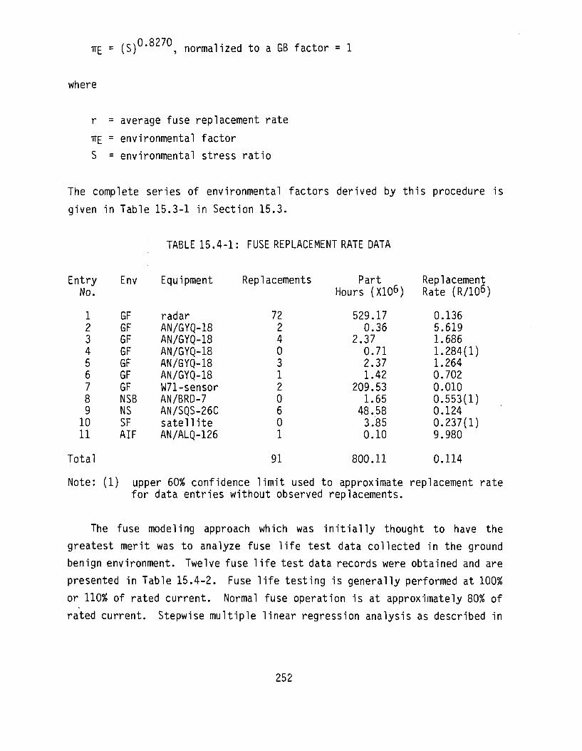
iTE = ( S ) 0 , 8 2 7 0 , normalized to a GB factor = 1
where
r = average fuse replacement rate
TTE = environmental factor
S = environmental stress ratio
The complete series of environmental factors derived by this procedure is
given in Table 15.3-1 in Section 15.3.
TABLE 15.4-1: FUSE REPLACEMENT RATE DATA
Entry No.
1 2 3 4 5 6 7 8 9 10 11
Env
GF GF GF GF GF GF GF NSB NS SF AIF
Equipment
radar AN/GYQ-18 AN/GYQ-18 AN/GYQ-18 AN/GYQ-18 AN/GYQ-18 W71-sensor AN/BRD-7 AN/SQS-26C satellite AN/ALQ-126
Replacements
72 2 4 0 3 1 2 0 6 0 1
Part Hours (X106)
529.17 0.36
2.37 0.71 2.37 1.42
209.53 1.65
48.58 3.85 0.10
Replacement Rate (R/106)
0.136 5.619 1.686 1.284(1) 1.264 0.702 0.010 0.553(1) 0.124 0.237(1) 9.980
Total 91 800.11 0.114
Note: (1) upper 60% confidence limit used to approximate replacement rate for data entries without observed replacements.
The fuse modeling approach which was initially thought to have the
greatest merit was to analyze fuse life test data collected in the ground
benign environment. Twelve fuse life test data records were obtained and are
presented in Table 15.4-2. Fuse life testing is generally performed at 100%
or 110% of rated current. Normal fuse operation is at approximately 80% of
rated current. Stepwise multiple linear regression analysis as described in
252
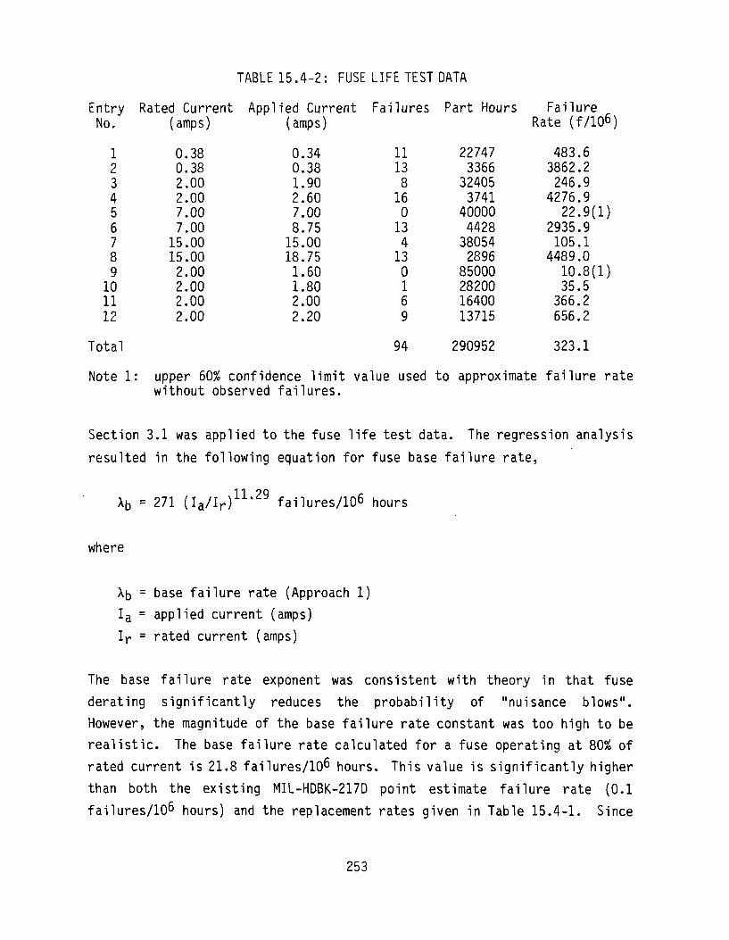
TABLE 15.4-2: FUSE LIFE TEST DATA
Entry No.
1 2 3 4 5 6 7 8 9 10 11 12
Total
Rated Current (amps)
0.38 0.38 2.00 2.00 7.00 7.00 15.00 15.00 2.00 2.00 2.00 2.00
Applied Current (amps)
0.34 0.38 1.90 2.60 7.00 8.75 15.00 18.75 1.60 1.80 2.00 2.20
Failures
11 13 8 16 0 13 4 13 0 1 6 9
94
Part Hours
22747 3366 32405 3741 40000 4428 38054 2896 85000 28200 16400 13715
290952
Failure Rate (f/106)
483.6 3862.2 246.9 4276.9 22.9(1)
2935.9 105.1
4489.0 10.8(1) 35.5 366.2 656.2
323.1
Note 1: upper 60% confidence limit value used to approximate failure rate without observed failures.
Section 3.1 was applied to the fuse life test data. The regression analysis
resulted in the following equation for fuse base failure rate,
Xb = 271 (I a / I r )1 1 , 2 9 failures/10^ hours
where
Xb = base failure rate (Approach 1)
Ia = applied current (amps)
Ir = rated current (amps)
The base failure rate exponent was consistent with theory in that fuse
derating significantly reduces the probability of "nuisance blows".
However, the magnitude of the base failure rate constant was too high to be
realistic. The base failure rate calculated for a fuse operating at 80% of
rated current is 21.8 failures/10^ hours. This value is significantly higher
than both the existing MIL-HDBK-217D point estimate failure rate (0.1
failures/10^ hours) and the replacement rates given in Table 15.4-1. Since
253

it is illogical for the fuse replacement rate to be lower than the failure
rate, this approach was considered invalid. Three possible explanations for
the failure of this approach to yield an acceptable model are:
(1) The life test conditions were not typical of field operating conditions. Additional operating stress caused by the particular test conditions could be responsible for the excessively high base failure rate constant.
(2) The relation between failure rate and fuse derating is a continuo s function but too complex to be determined from the available data.
(3) The relation between failure rate and fuse derating should not be represented by a continuous function. Failure rate as a function of fuse derating hypothetically could be best represented by a step function. The failure rate may increase gradually with increased applied current until a point near unity (Ia/Ir = 1) where the failure rate increases dramatically.
The failure of the initial approach to produce a usable failure rate
prediction model resulted in the development of several alternate
approaches. The second approach was based on analysis of the ratio of
replacement rate to failure rate. It is known that the replacement rate is
greater than or equal to the failure rate for e\/ery conceivable fuse
application. This must be true because a system normally cannot operate with
a failed fuse in-place and therefore it must be replaced. It must also be
true that the ratio of replacement rate to failure rate must be greater than
or equal to one. In equation form, the relationships between replacement
rate and failure rate are given by:
H > xi
^> 1-0
where
r-j = replacement rate of the itn data entry
254
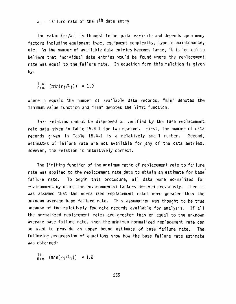
Xi = failure rate of the itn data entry
The ratio (r-j/X-j) is thought to be quite variable and depends upon many
factors including equipment type, equipment complexity, type of maintenance,
etc. As the number of available data entries becomes large, it is logical to
believe that individual data entries would be found where the replacement
rate was equal to the failure rate. In equation form this relation is given
by:
r S (min(ri/Xi)) = 1.0
where n equals the number of available data records, "min" denotes the
minimum value function and "lim" denotes the limit function.
This relation cannot be disproved or verified by the fuse replacement
rate data given in Table 15.4-1 for two reasons. First, the number of data
records given in Table 15.4-1 is a relatively small number. Second,
estimates of failure rate are not available for any of the data entries.
However, the relation is intuitively correct.
The limiting function of the minimum ratio of replacement rate to failure
rate was applied to the replacement rate data to obtain an estimate for base
failure rate. To begin this procedure, all data were normalized for
environment by using the environmental factors derived previously. Then it
was assumed that the normalized replacement rates were greater than the
unknown average base failure rate. This assumption was thought to be true
because of the relatively few data records available for analysis. If all
the normalized replacement rates are greater than or equal to the unknown
average base failure rate, then the minimum normalized replacement rate can
be used to provide an upper bound estimate of base failure rate. The
following progression of equations show how the base failure rate estimate
was obtained:
All (mintri/X-j)) = 1.0
255

rwl2 (min(riAb)) >. 1-0
The average base failure rate can be factored out of the minimum value
function because it was assumed to be a constant value.
(min(ri))/Xb >, 1.0
Xb <_ min (r-j)
The minimum normalized replacement rate was data entry number 7 in Table
15.4-1. Therefore, the estimate for base failure rate is:
X"b < .010 * 2.3 = 0.00435 f/106 hours
where
normalized replacement rate of itn data entry
normalized failure rate of i^n data entry
average base failure rate
environmental factor for GF.
Multiplication of the average base failure rate value by the environmental
factor completed the model development for this approach. The inherent
difficulty with this approach is the use of several assumptions which can
neither be proved or disproved. Also, the derived numerical base failure
rate value ultimately is based on one data record. Therefore, extensive data
quality control is required for proper application of this approach.
A third approach was deemed necessary because of the inadequacy of the
first approach and the uncertainty of the second approach. This third
approach assumed a fuse failure rate prediction model of the form:
Xp = Xb x TIE
*i =
*b =
2.3 =
256

where
Xp = predicted fuse failure rate
Xb = base failure rate = constant value
TIE = environmental factor (Table 15.3-1)
The basis of the third approach was the assumption that the existing MIL-
HDBK-217D average point estimate failure rate was an accurate measure of the
average observed failure rate of data entries from a variety of application
environments. This assumption was believed to be accurate because most of
the criticism by reliability analysts was that the current model did not
sufficiently discriminate against fuse reliability characteristics and not
that the current model was an inaccurate measure of the average fuse failure
rate. The data collected in support of this study (Table 15.4-1), r = 0.114
R/106 hours, also did not disprove this assumption. To derive the base
failure rate value, the average fuse failure rate for the eleven environment
categories included in MIL-HDBK-217C was assumed equal to the existing MIL-
HDBK-217D average failure rate value of 0.1 failures/106 hours. The eleven
environmental categories were used instead of the current 26 environments
because the original use of the 0.1 value was not intended for such stressful
environments as cannon,launch and underwater, sea launch. Therefore the base
failure rate was obtained by:
, in 0.1 failures/106 hours = ± Z (Xb TTE)
n i=1
0-1 = if (xbU-0 + 2.3 + 7.5 + 5.2 + 10 + 6.8 + 12 + 13 + 18 + 1.8 + 22))
X b = 11(0.1) (1/99.6)
= 0.0110 failures/106 hours.
Neither approach two nor three had enough merit to be the sole basis of a
failure rate prediction model. However, the relative proximity of the base
failure rate values obtained from approaches two and three was sufficient
justification for proposing a revised failure rate prediction model for
257
fuses. The base failure rate value obtained from approach three was included
in the proposed model because it was the larger of the two values.
The proposed fuse failure rate modeling approaches described in this
section present several attempts at deriving an equation for fuse failure
rate. It was encouraging that two of the three modeling approaches yielded
similar failure rate prediction models because of the severe field failure
rate data collection problems associated with fuses.
15.5 Bibliography
Arno, R.G., Nonelectronic Parts Reliability Data, RAC publication NPRD-2, Summer, 1981.
Backe, R.J., Evaluation of Screening Methods to Obtain Long Life Subminiature Picofuses, Goddard Space Flight Center report no. PACER 04-004, November, 1980.
Ross, M., Corrosion Resistance of Silver Plated Copper and Brass Versus Unplated Copper and Brass, Federal Pacific Electric Co. Internal Report, August 1978.
Thomas E., The Mechanisms of Degradation and Failure in a Filamentary Fuse Wire, Goddard Space Flight Center report no. FMR 04-003, May, 1972.
258
16.0 QUARTZ CRYSTALS
16.1 Device Description
A crystal unit is an assembly which consists of a quartz resonator
suitably mounted in a crystal holder. Quartz crystals are manufactured in a
wide variety of mounting and holder configurations to suit many
applications.
Quartz is useful in the electronics field because it is piezoelectric and
has stable physical properties and manageable behavior over wide temperature
ranges. The piezoelectric effect causes an electrical potential difference
between two opposite faces of a quartz plate when the plate is mechanically
stressed. Conversely, when a potential difference is applied to the two
opposite sides of the quartz plate, mechanical stress and movement are
generated.
Quartz plates which are cut to proper dimensions and appropriately
mounted will vibrate in mechanical resonance at the desired frequency if an
alternating voltage is applied to the opposite crystal faces. The unusually
high stiffness and elasticity of this very hard crystalline material make it
possible to produce electromechanical resonators that will operate over a
wide range of frequencies extending from approximately 1000 Hertz to 150
Megahertz.
Figure 16.1-1 shows typical mounting variations used by various crystal
manufacturers for a 1 MHz AT cut crystal in the standard MIL-HC-6/U holder.
Figure 16.1-2 presents the construction and mounting of a larger low
frequency crystal device. Figure 16.1-3 shows a typical edge-clamped mount
which is widely used for mounting high frequency crystals. Electrodes are
plated on the opposite crystal surfaces with the plating extended to opposite
edges to provide attachment to the mounts. The crystal faces are only
partially plated so that the effective electrode area is confined to a small
circular region at the center of the blank. Thus, the capacitance is kept to
259

r j j * * 5 ^ ^ ^
f i ! j
! 1
1
1
u
if
rt
-a v-
L FIGURE 16.1-2: TYPICAL MOUNTING
OF A LOW FREQUENCY CRYSTAL
FIGURE 16.1-1: TYPICAL MOUNTING
VARIATIONS FOR A 1MHz CRYSTAL
FIGURE 16.1-3: CEMENTED LEAD
MOUNTING FOR HIGH FREQUENCY CRYSTALS
260
a minimum and the principal activity is confined to the center of the crystal
where it is most likely to be of uniform thickness. Both these factors
contribute to frequency stability. The mounting wires are clamped and
cemented at the edges, where activity of the crystal is low.
For high levels of shock and vibration, the wire mounts shown in Figure
16.1-3 are replaced by stiffer channel shaped mounts to keep the mount
resonant frequency above 2 or 3 KHz. This ruggedized mounting requires some
sacrifice in temperature stability and aging characteristics.
The most recent developments in crystal holders are in the use of cold-
welded cases and internal ribbon mounts. The cold-welded process eliminates
exposure of the crystal to high temperatures and/or solder flux contaminants
which can occur with the use of glass enclosures and conventional solder-
sealed cans. The use of a ribbon mount, as developed by Bell Telephone
Laboratories, satisfies the requirement of high mount resonant frequency
without inducing stress in the crystal blank.
One version of this type of internal ribbon mount employs three short
ribbons which position the blank parallel to the base of a standard TO-5 can.
In theory, three short ideal ribbons will remove the six degrees of freedom
of the blank without any redundancies. In practice, this type of mount has
resulted in a reduction of two orders of magnitude in vibration sensitivity
as compared to the standard wire mount. At the same time, aging
characteristics are not degraded and the lowest resonant frequency of the
assembly is well above 2000 Hz. This type of mount appears to be
particularly suited for high frequency applications where vibration
modulation sensitivity is of concern.
16.2 Failure Modes and Mechanisms
Quartz crystals, if properly applied, are among the most reliable of
electronic components. Wearout failure mechanisms associated with operation
of a quartz crystal are observed rarely when operated within its design
261
specifications. An example of a wearout failure mechanism which does occur
is frequency drift. The majority of crystal failures can be categorized as
catastrophic failures. There is a continuous aging process which decreases
exponentially with time.
Operation above rated drive level will result in deterioration of
stability, even though the dissipation is well below the level at which the
crystal may shatter. High drive level will also accelerate the normal aging
characteristics.
There are certain failure mechanisms associated with manufacturing which
may or may not be detected prior to equipment installation. These failure
mechanisms can result in either catastrophic failure or excessive drift
after some period of operation. Some of the more common defects are listed
below:
o Poor seal
o Excessive contamination
o Excessive internal mechanical stresses introduced by the blank mounting structure
o Poor electrical connections
A poor seal will result in a gradual frequency drift and an increase in
crystal resistance due to entrance of moisture and other surface
contaminants. The crystal may fail either by drifting out of tolerance or by
an increase in resistance to the point that it may no longer oscillate.
The effect of excessive contamination is the same as that of a poor seal
except that the contaminants are already present at the time of manufacture.
This defect is relatively rare among quality manufacturers and the use of
cold welded cases reduces the problem of contaminants, such as solder flux,
being introduced during the sealing operation.
262
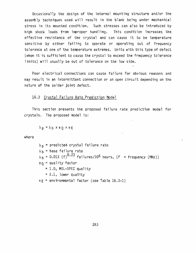
Occasionally the design of the internal mounting structure and/or the
assembly techniques used will result in the blank being under mechanical
stress in its mounted condition. Such stresses can also be introduced by
high shock loads from improper handling. This condition increases the
effective resistance of the crystal and can cause it to be temperature
sensitive by either failing to operate or operating out of frequency
tolerance at one of the temperature extremes. Units with this type of defect
(when it is sufficient to cause the crystal to exceed the frequency tolerance
limits) will usually be out of tolerance on the low side.
Poor electrical connections can cause failure for obvious reasons and
may result in an intermittent connection or an open circuit depending on the
nature of the solder joint defect.
16.3 Crystal Failure Rate Prediction Model
This section presents the proposed failure rate prediction model for
crystals. The proposed model is:
where
X p = X b XTTQ XTTE
Xp = predicted crystal failure rate
Xb = base failure rate
Xb = 0.013 ( f ) 0 , 2 3 failures/106 hours, (f = frequency (MHz))
TTQ = quality factor
= 1.0, MIL-SPEC quality
= 2.1, lower quality
TTE = environmental factor (see Table 16.3-1)
263
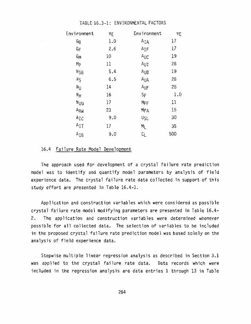
TABLE 16.3-1: ENVIRONMENTAL FACTORS
Environment
SB
GF
GM
Mp
NSB NS Nu
NH NUU ARW
AlC AIT
TTE
1.0
2.6 10
11 5.4
6.5
14
16 17
23 9.0
17
Environment
AlA
AlF AUC AUT
AUB
AUA
AUF
SF
MFF
MFA
USL
ML
TfE 17
17
19
28
19
28
28
1.0
11
15 30
35
A I B 9.0 CL 500
16.4 Failure Rate Model Development
The approach used for development of a crystal failure rate prediction
model was to identify and quantify model parameters by analysis of field
experience data. The crystal failure rate data collected in support of this
study effort are presented in Table 16.4-1.
Application and construction variables which were considered as possible
crystal failure rate model modifying parameters are presented in Table 16.4-
2. The application and construction variables were determined whenever
possible for all collected data. The selection of variables to be included
in the proposed crystal failure rate prediction model was based solely on the
analysis of field experience data.
Stepwise multiple linear regression analysis as described in Section 3.1
was applied to the crystal failure rate data. Data records which were
included in the regression analysis are data entries 1 through 13 in Table
264
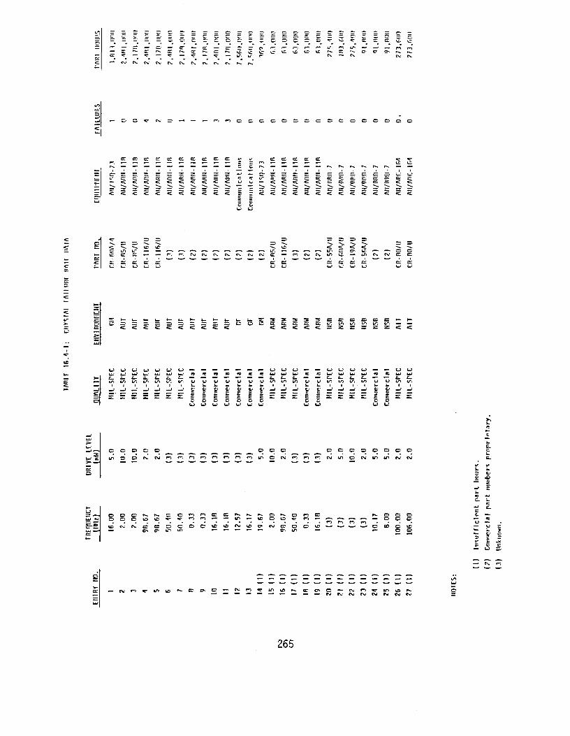
= e> =
— c — G c c c
— «e- —
l — T ' — L T - f ^ L P — — —
Cs. — Cs.
— O G ^ r t v o — — ~- G C G G O G G O G C O O O O G O
cr c c: c c c c: rr rr cr c:
ri111111111 ss^ i i i i i l i i i i i i g < ; < ; < ; < ; < ; < ; < : < ; < ; < ; < ; s <:< :< :< :< :< :< :< :< :< :< :< :< :< :
^ c c= — — £ £ c c e
r -. rw tv cs. rv
<-> ^ i_)
? * 5 = l/*, f ) Lfl f l 1/1 l/". — —
«— — o o — «—
i/i to to to i/v
Ill £1 CJ _ J - J
to m v< m u i i i i k .
- J - j _ i _ • & G» _ J _J
= = E | = = S
G- o C\J C\J n
O O O
«•*> n i n O c J
G G C G O G G O r \ j i r > o c s j i r > m c s j c s j
£ -£>
O *- «^ G G
o c c m M G \D «—
c A J
c c u
r> t r
—
C
to
u -f s = o i_>
= X o = .* c =
265

TABLE 16.4-2: QUARTZ CRYSTAL CONSTRUCTION AND APPLICATION VARIABLES
I. Mode of Oscillation A. Fundamental B. Third Overtone C. Fifth Overtone
II. Frequency
III. Load Capacitance
IV. Quartz Plate Dimensions
V. Rated Drive Level
VI. Type of Cut A. AT B. BT C. CT D. DT E. NT
VII. Construction Options A. Cold-Welded Cases B. Internal Ribbon Mount
VIII. Mounting and Holder Configuration
IX. Operating Temperature A. Rated
B. Actual
X. Application Environment
XI. Manufacturing Quality Level
266

16.4-1. Other data records included insufficient part hours to estimate a
failure rate without observed failures. The regression analysis resulted in
the following crystal failure rate prediction model.
Xp = Xb x TTQ x TTE
where
Xp = predicted crystal failure rate in failures/10^ hours
Xb = base failure rate
Xb = 0.0306 ( f )0 - 2 3 4 failures/106 hours, (f = frequency (MHz))
TTQ = quality factor
= 1.0, MIL-SPEC quality
= 2.1, lower quality
TIE = environmental factor = 1.0, GF
= 4.4, GM
= 9.3, AUT
= 9.6, AUF
It should be noted that the base failure rate constant given above differs
from the value given in section 16.3. This apparent discrepancy is due to
normalization of the environmental factors. The regression analysis assumed
a ground fixed environmentil factor equal to one because no data were
available from a ground benign environment. The proposed crystal failure
rate prediction model environmental factors were normalized to a ground
benign factor equal to one to be consistent with existing MIL-HDBK-217D
models. The details of the regression analysis are given in Table 16.4-3.
Base failure rate, quality factor and environment factor were defined by the
following equations:
*b = (exp(bo)) (f) b 2
TTQ = exp(b3X3)
267
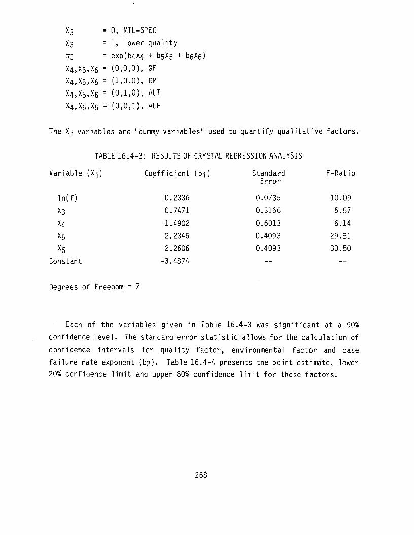
X3 = 0, MIL-SPEC
X3 = 1, lower quality
TTE = exp(b4X4 + b^s + D6X6)
X4,X5,X6 = ( 0 , 0 , 0 ) , GF
X4,X5,X6 = ( 1 , 0 , 0 ) , GM
X4,X5,X6 = ( 0 , 1 , 0 ) , AUT
X 4 , X 5 , X 6 = ( 0 , 0 , 1 ) , AUF
The X-j variables are "dummy variables" used to quantify qualitative factors.
TABLE 16.4-3: RESULTS OF CRYSTAL REGRESSION ANALYSIS
Variable (X-j) Coefficient (b-j)
ln(f) 0.2336
X3 0.7471
X4 1.4902
X5 2.2346
X6 2.2606
Constant -3.4874
Degrees of Freedom = 7
Each of the variables given in Table 16.4-3 was significant at a 90%
confidence level. The standard error statistic allows for the calculation of
confidence intervals for quality factor, environmental factor and base
failure rate exponent (b2). Table 16.4-4 presents the point estimate, lower
20% confidence limit and upper 80% confidence limit for these factors.
Standard Error
0.0735
0.3166
0.6013
0.4093
0.4093
F-Rati
10.09
5.57
6.14
29.81
30.50
268

TABLE 16.4-4: CONFIDENCE INTERVALS FOR CRYSTAL PARAMETERS
Parameter
Xb exponent
TTQ, MIL-SPEC
TTQ, lower
TTE, GF
TTE, GM-
TT£, ALIT
TTE, AUF
PT EST
0.234
1.0
2.11
1.0
4.44
9.34
9.59
L 20% CL
0.169
1.60
2.62
6.53
6.70
U 80% CL
0.298
2.79
7.52
13.37
13.72
Analysis of the data allowed for determination of only four
environmental factors. To improve the utility of the proposed model, a
complete series of environmental factors was determined. There is no part
type current]y included in MIL-HDBK-217D whose environmental factors
adequately represent the effects of environmental stress on crystals.
Therefore, the methodology described in Section 3.3 was applied to the four
observed environmental factors to derive an applicable series of factors.
This method assumes that an environmental factor relation can be determined
where environmental factor is a function of the "environmental stress
ratios" given in Reference 1. The results of the environmental factor
derivation are given by the following equations.
TTE1 = 0.4105 (S) 0.9448
TTE2 = (S) 0.9448
where
TTEI = environmental factors normalized to a ground fixed TTE = 1
TTE2 = environmental factors normalized to a ground benign TTE = 1
S = environmental stress ratio
269

It was considered desirable for the environmental factors included in
the proposed crystal failure rate prediction model to be normalized to a
ground benign factor equal to one. The preliminary failure rate prediction
model obtained by the regression analysis was normalized to a ground fixed
environmental factor equal to one. Therefore, the base failure rate constant
given previously in this section was multiplied by a factor of 0.4105 and the
appropriate set of environmental factors U E 2 ) was included in the proposed
model. Thus, the equation for base failure rate becomes,
Xb = 0.0126 ( f ) 0 - 2 3 4 failures/106 hours
The complete set of environmental factors normalized to a ground benign
factor equal to one is presented in Table 16.3-1.
Normalization of the base failure rate and the environmental factors
concluded the failure rate prediction model development for crystals. The
existing MIL-HDBK-217D failure rate prediction model for crystals consists
of.a single point estimate for all applications. The proposed model presents
failure rate as a function of frequency, quality level and application
environment and use of this proposed model will improve the reliability
prediction capabilities for equipments designed with quartz crystals.
16.5 References and Bibliography
References
1. Kremp, B.F. and E.W. Kimball, Revision of Environmental Factors for MIL-HDBK-217B, RADC-TR-80-299, September 1980.
Bibliography
Fink, D.G. and D. Christianson, Electronics Engineers Handbook, Section 7, Second Edition, McGraw-Hill, 1982.
270

17.0 LAMPS
17.1 Incandescent Lamps
17.1.1 Device Description
Tungsten filament incandescent lamps are used extensively as miniature
and subminiature indicator lamps. Construction options such as bulb size,
filament type, light output, rated voltage and rated current are available in
numerous combinations such that the optimal incandescent lamp type can be
chosen for any particular application. Incandescent lamps are generally
constructed of an envelope, a filament, a filament support, lead wires, a
bead, an exhaust tip and a lamp base.
The envelope is commonly made of clear or colored glass. Envelopes for
some high-powered lamps may be made of quartz or high-temperature glass. The
envelope shape is coded by letter and by diameter in one eighth inch units.
The letter codes used to specify envelope shape are T, 6, S, B and RP
corresponding to tubular, globular, straight-sided, blister, and pear-shaped
reflector respectively. For example a T-2 bulb would be tubular with a
diameter of two times one eighth inch (equal to one quarter inch).
Filaments can be classified into three categories. In general filaments
are either coiled (coded C), straight (coded S) or coiled-coil (coded CC).
The coiled type is more thermally efficient than the straight wire because
heat can not escape as readily and therefore the filament becomes hotter for
the same current. Filament supports are sometimes needed for the longer
filaments which are required in high voltage, low current lamps. The
supports cool the filament in their vicinity but are a liability in regard to
vibration and filament notching.
Lead wires are low-resistance conductors usually having three purposes.
They conduct electricity to the filament, they provide part of the filament
support, and they carry the electricity through their mechanical seal with
271

the envelope glass. The connection to the filament is usually a crimp or a
weld. Their ability to support the filament is improved by being short
because the mechanical response to vibration is reduced. The thermal
coefficient of expansion of the lead wire material must match the thermal
coefficient of expansion of the glass through which they pass, or repeated
heating and cooling of the lamp would soon fracture the seals. Having a hot
filament at one end is most compatible with long internal lead wires, so the
glass and the wire may change temperature gradually and simultaneously.
Selection of the lamp internal lead length requires a compromise between
shock/vibration response and seal-heating requirements.
The lamp bead provides a means of supporting the filament assembly both
before it is mounted in the envelope and afterwards. Color of the bead
offers a means of lamp identification.
The exhaust tube is used to evacuate the lamp. Most lamps have the
filament in a vacuum. This reduces the loss of heat from the filament and
produces more light output for the same filament current or applied voltage.
Occasionally lamps are back-filled with argon, an argon-nitrogen mixture or
another gaseous mixture to reduce tungsten evaporation from the filament.
This will increase lamp life and reduce blackening within the envelope.
Lamp bases are commonly cemented to the envelope. The lead wires are
usually soldered to the contacts. Use of soft solder is common though there
is some advantage in the use of higher-temperature solders. In other cases a
welded connection is made. The lamp base makes both electrical and
mechanical contact to the equipment in which the lamp is installed. The base
also provides a dimensional reference to the "light center".
Incandescent lamps are commonly used under high ambient light conditions
as on-off indicator lights and for the internal illumination of panels in
military equipment. They are used as the light source in projection alpha
numeric readouts, as well as the segment types of readout. Occasionally they
272

are used in pulsing or flashing circuits, and they may be used as a current-
sensitive resistor in electronic circuits, such as automatic gain controls.
17.1.2 Failure Modes and Mechanisms
In AC operation, the predominant failure mechanism of an incandescent
lamp is evaporation of the tungsten filament. Unlike most electronic
devices, the lamp filament must be in a deterioration mode to operate (i.e.
to illuminate). Ideally, the filament evaporates uniformly and the light
intensity of the lamp gradually fades. In practice, however, the evaporation
of the filament is not uniform and weak spots in the filament develop.
Notching is the term generally used to describe this phenomenom of nonuniform
evaporation of the filament. Failures are observed in the weak spot area
when exposed to mechanical shock and/or vibration.
Several factors may increase the number of observed notching type
filament failures. Higher voltage incandescent lamps require a longer,
thinner filament. The thinner filament is more susceptible to failures
induced by notching because the size of the notch and the rate of increase of
the notch size are independent of filament diameter. Additionally filaments
in high voltage lamps require filament supports becuase of their more fragile
construction. The presence of the filament supports also tend to accelerate
notching. The observed failure rate of incandescent lamps would be expected
to be highly correlated to the rated voltage because of these factors.
Another factor influencing the evaporation rate of the filament is the
ratio of applied voltage to rated voltage. As the ratio of applied to rated
voltage is increased, internal lamp temperature is increased and the
evaporation of the filament is accelerated. Lamp failure rate is related
directly to filament evaporation rate.
In DC operation an additional failure mechanism is introduced which is
dominant. DC operation results in electromigration of the tungsten filament
in the direction of the applied electric field. Electromigration of the
273
tungsten in one direction reduces the minimum filament diameter. This
increases the susceptibility of the lamp to failures from exposure to shock
and/or vibration.
The life of an incandescent lamp relative to the life of the equipment in
which it is installed is highly dependent on duty cycle. While the lamp is
illuminating, the filament is in the process of evaporating and the average
failure rate (in units of failures per equipment hr.) is relatively higher.
Therefore the particular application of the incandescent lamp is of extreme
importance in regard to the reliability. Applications for incandescent
lamps range from a duty cycle of 1.0 (i.e., power on indication, constant
illumination of dial/meter) to duty cycles approaching zero for certain
warning indicator lamps. Generally the duty cycle of an incandescent lamp to
be used as a warning indicator is unknown in the reliability prediction phase
of equipment design.
Environmental stresses such as shock and vibration shorten lamp life by
inducing failures in areas of the filament which have been weakened by either
uniform evaporation, notching or electromigration of the filament.
Therefore, application environment would be anticipated to have a
significant effect on incandescent lamp failure rate. However, proper
incandescent lamp selection can minimize the effects of the environment.
Incandescent lamp manufacturers often offer lamps with similar
specifications but different intended applications.
The instantaneous failure rate of an incandescent lamp is expected to be
very time dependent. The dominant failure mechanisms for both AC and DC
operation are degradation mechanisms such as uniform evaporation of the
filament and filament notching. Collection of field experience data which
allows analysis of failure rate time dependence is difficult and accurate
estimates of Weibull or normal failure rate distribution parameters can not
be determined.
274
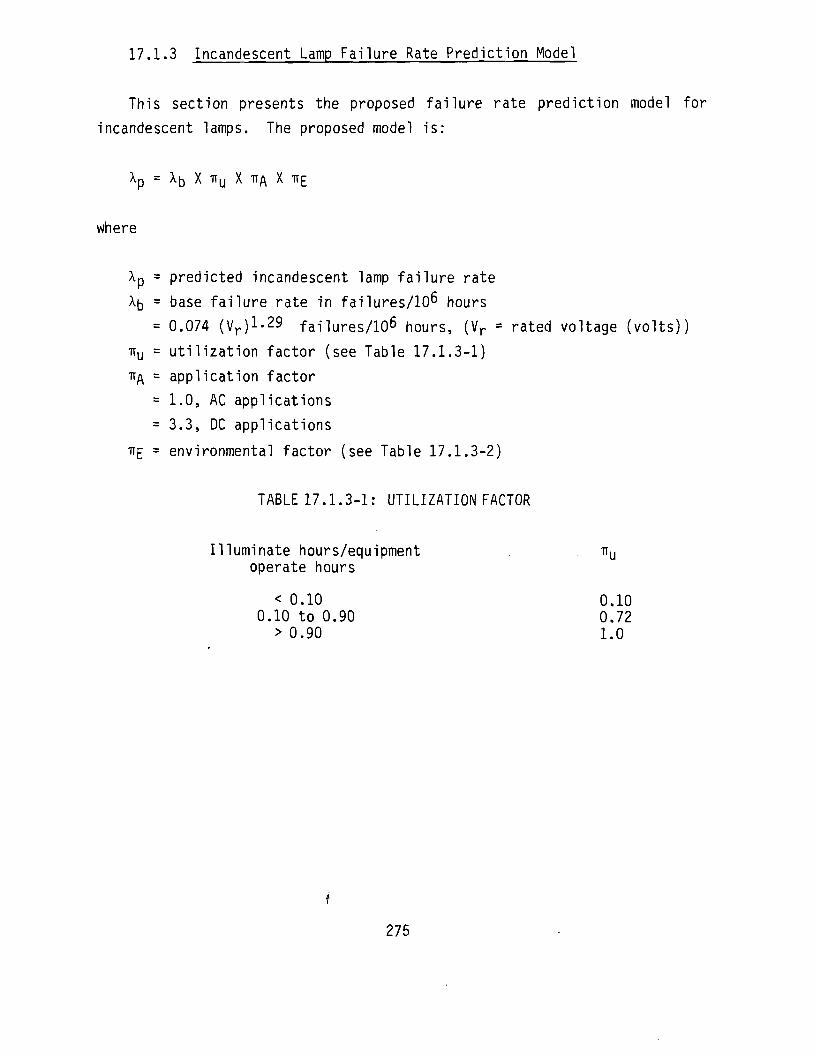
17.1.3 Incandescent Lamp Failure Rate Prediction Model
This section presents the proposed failure rate prediction model for
incandescent lamps. The proposed model is:
X p = Xfo X TTU X TT/\ X TT£
where
Xp = predicted incandescent lamp failure rate
X5 = base failure rate in failures/106 hours
= 0.074 (Vr)!-29 failures/106 hours, (Vr = rated voltage (volts))
TTU = utilization factor (see Table 17.1.3-1)
TT/\ = application factor
= 1.0, AC applications
= 3.3, DC applications
TTE = environmental factor (see Table 17.1.3-2)
TABLE 17.1.3-1: UTILIZATION FACTOR
Illuminate hours/equipment TTU operate hours
< 0.10 0.10 0.10 to 0.90 0.72
> 0.90 1.0
275

TABLE 17.1.3-2: ENVIRONMENTAL FACTOR
Environment
6B GF
6M Mp
NSB NS Nu
NH NUU ARW
AlC AIT
AlB
TTE
1.0
1.6 3.4
3.5 2.4
2.7
4.1
4.4
4.5
•5.3
3.2 4.4
3.2
Environment
AlA
AlF
AUC AUT
AUB AUA
AUF
SF
MFF MFA
USL
ML
CL
TTE
4.4
4.4
4.8
5.8
4.8
5.8
5.8
1.4
3.5
4.2
6.1
6.5 27
17.1.4 Failure Rate Model Development
The methodology used to develop a failure rate prediction model for
incandescent lamps included parameter identification and quantification by
analysis of life test data, field experience data and theoretical
reliability studies. The failure rate data collected in support of this
study effort is given in Table 17.1.4-1.
As a prerequisite to collection of life test and field experience data, a
list of construction and application variables were determined for
incandescent lamps. The construction and application variables represent
possible failure rate model parameters whose values were determined for all
collected data whenever possible. The construction and application
variables are given in Table 17.1.4-2.
276
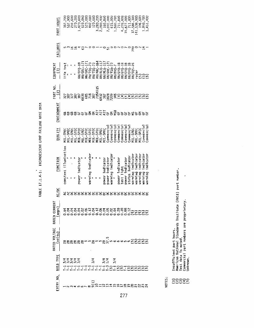
o o o o o o o o o o o o o o o o o o o o o o o o o o o o o o o o o o o o o o o o o o o o o o o o s c j n D M \ D o o o o r s n T c o o O M » c ; o c o n c j n £ ) N < T c \ i N o ^ n n n n c \ j n n o o c j L n O ' - ( O N ' H ^ c o ^ c o - H C 0 a ^ L n ' ^ c ^ J C ^ J C ^ J a ^ c ^ J C 0 o ^ ^ t ^ ^ H ' ^ D ^ H ^ ^ ^ ^ • - | C 0 ' , ^ O , . C T I L T I
- H <=- o ^ H n c
vo in O
CO 0 0 CO CO VD
I I I I I I I t I I I I I I > I
U C 3 U I - h < « i < U I - m U C 3 U C 3 W ro
r x r ^ r x r ^ r x p M n c o r ^ i r c v j r x c o c ^ i r -— -— -— -— <— <— <— <— -— c \ jcoe\ jcocomco«—• co • — ' n c o c s j o ^ w w i n i D i n i n i n
C U C 3 0 0 U C 3 0 C 3 < < < C 3 C 3 Z U C 3 U C 3 2 C 3 C 5 U C 3
1 s fO fO ID fO ID (D <C <D (O
O O O O O O O O O O O O " - * • - • » - • • - • • - • • - • ' - <_J <_J O • » - f -L U L U L L J L L J L L J L L J L I J L L J L L J L L J L L J L I J ( J ( J ( J ( J ( J ( J ( J L L J U J U J ( J ( J D - Q . C D - O . Q . 1 1 D . C . D - G . C L L- 1 - t - k. 1 - i- 1 - Q . D_ D_ L. k. ( / ) l / 1 l / ) l / 1 l / l l / H / l ( / ) ( / H / l l / ) i O QJ QJ (D (D QJ QJ Q) I / ) LO I r t QJ QJ
i i i i i i i i i i i I E E E E E E E ' i i E E — i — i — i — i — i — i — i — i — i — i — i I = = E E E E E — i — i — i £ E _ _ _ _ _ « _ _ _ — . — . _ _ o O O O O O O ^ — <—• O O
(D f -
k. f -OJ =
O
fc. fc. fc. J - i . fc. O 1 - O O O O O
= k. k. 4-> = k. L. o *-> *-> •*->•*-> •*-> O O »D O O ^ V i t iC >C Q
4_» 4-» ( J 4-> + J ID ( J U U U ( J ID IO • • - »D I D U • » - • » - i - — f -(J ( J " O (J (J • • - " O " O " O " O " O
" C J " C J f - - D ^ " D C f - f - f - f - f -
• ^ • ^ O l - ^ - ^ f— D d O ) O ) W C — i n C C C C C
k. k. f - J - k. 3 t - t - • - - * ^ • - -= QJ QJ C = Q J - M Q J 4 - > C C C C C
3 3 k. J i n j i c l . l . l , l . t O O ID O Q I O ^ i D Q Q i Q i ? D . D . 5 D -4 -» D . W X X 3 5 X
= J D . O E
W W T N » £ > N V f M l D * T l f i C V J C O O C O N 0 0 0 0 0 0 0 ^ 0 — « O O O O O C \ J C \ J O ^ # - ^ # - ^ # - ^ * ~ « - ^
in in in in m
o o o o o o o o o o o o o o o o o o o *—»—*—*—*_-
CO
^- ^- r r ^- ^ ^ «r ^- *r
-- --* --* -- -- -- -- -- * . i i i i > i i i i i i i i i n i m m i i n i n i n i n i n i n
* <D k. C k. 3 ID QJ O *•> . Q
£ W • E
4-> . — QJ C J - (D - M m c o •*-» Q . O C k.
•.- m 4-> 4-> w a. C (O f -ai -z. r-•f- m <D U C - M • • - .
T- to m v c **- u -a k. 5 *» - ^ - QJ O =S k. - M g C V) OJ v i E ^ C E OJ O C
• - • < t— t_) = )
^ w n r i n -—-O M f v j n f l - i n v D i ^ c o o ^ O ' ^ f v j n f l '
*CNjro^-invor^coo^'—••—•.—•.—•«—•.—•.—•.—•,—».—• C\J CM C\J CM csi
277

TABLE 17.1.4-2: INCANDESCENT LAMP CONSTRUCTION AND APPLICATION VARIABLES
I• Type A. Large B. Miniature C. Subminiature D. Ultraminiature
II. Bulb Shape A. Globular B. Straight Side C. Tubular D. Other
III. Filament Type A. Coiled B. Straight C. Coiled-Coil
IV. Voltage Level A. Rated B. Actual
V. Current Level A. Rated B. Actual
VI. Function A. Light Source B. Power Indicator C. Warning Indicator D. Test Light E. Status Indicator
F. Other
VII. Ratio of Illumination Time to Equipment Operating Time
VIII. Number of "On-Off" Cycles per Unit Time
IX. Application Environment
X. Operating Temperature A. Rated B. Actual
XI. Manufacturing Qaulity Level
278
The hazard rate of incandescent lamps would be anticipated to be
increasing with time. However, incandescent lamp field experience data
which allows for investigation of a time dependent failure rate model was not
available. Therefore, average failure rate values were calculated for each
data entry with observed failures by dividing the number of failures by the
recorded part hours. An upper 60% confidence limit was used to approximate
failure rate for the data entries without observed failures. These failure
rates are equal to the catastrophic lamp failure rate plus an average wearout
failure rate contribution.
Stepwise multiple linear regression analysis (described in Section 3.1)
was applied to the incandescent lamp failure rate data. All data records
except entry number 9 in Table 17.1-4-1 were entered into the regression
analysis. Data entry number 9 had insufficient part hours to estimate a
failure rate without observed failures. The rated voltage and rated current
were unknown for data entries 20 through 24. An average rated voltage of
twelve volts was assumed for these data entries. This assumption may
slightly effect parameter estimation precision but was necessary to fully
evaluate all factors influencing failure rate. The rated voltage and rated
current were available for approximately 80% of all collected data and
therefore any detrimental effects from this assumption are minimal.
The lamp utilization presented a unique problem in application of
regression analysis. Generally a factor based on part utilization would be a
function of a quantitative variable like duty cycle. However, the duty cycle
of lamps used as warning indicators and test lights is unknown although
thought to be relatively low (<0.10). The duty cycle of lamps functioning as
status indicators is both unknown and variable over a range of values. The
duty cycle of lamps functioning as power indicators is known to be
approximately one. However, a factor could not possibly be based on this
information. Therefore, the lamp utilization was treated as a qualitative
variable similar to quality level or environment. "Dummy variables" of one
and zero were used in the regression analysis to represent applications with
periodic illumination and constant illumination respectively. Only one data
279

record was collected where a lamp functioned as a status indicator (data
entry #19 in Table 17.1.4-1). Therefore, analysis of this type of lamp
application could not be investigated by the regression analysis. The
failure rate of status indicator lamps is considered later in this section.
Treatment of lamp utilization as a qualitative variable not only aids the
reliability modeling analyst but would also aid a reliability engineer
performing an equipment reliability prediction. Reliability engineers using
a proposed incandescent lamp failure rate prediction model would not have
access to a precise measure of the anticipated duty cycle of a lamp
functioning as a warning indicator. Therefore, a fixed numerical quantity
for all warning indicator applications would provide maximum utility of the
failure rate prediction model.
Both rated voltage and rated current were not included in the regression
analysis because of a large negative correlation between the two variables.
A properly applied regression analysis should include only variables which
are independent. Rated voltage was chosen to be included in the analysis
based on theoretical considerations.
The details of the regression analysis are given in Tables 17.1.4-3 and
17.1.4-4. Table 17.1.4-3 defines the variables introduced into the
regression analysis and Table 17.1.4-4 presents the results of the analysis.
Variables which are included in Table 17.1.4-3 but not Table 17.1.4-4 are
those which could not be determined to have a significant effect on failure
rate. An explanation of quantitative and qualitative regression is included
in Section 3.1.
The results of the regression analysis indicate that bulb shape and
quality level do not significantly effect the observed failure rate.
This does not imply that quality level has no effect on failure rate.
However, the relative difference in failure rate between MIL-SPEC and
commercial quality incandescent lamps could not be distinguished from the
data. Additionally only two out of five environmental factor variables were
determined to be significant. These results are scrutinized in the following
paragraphs.
280
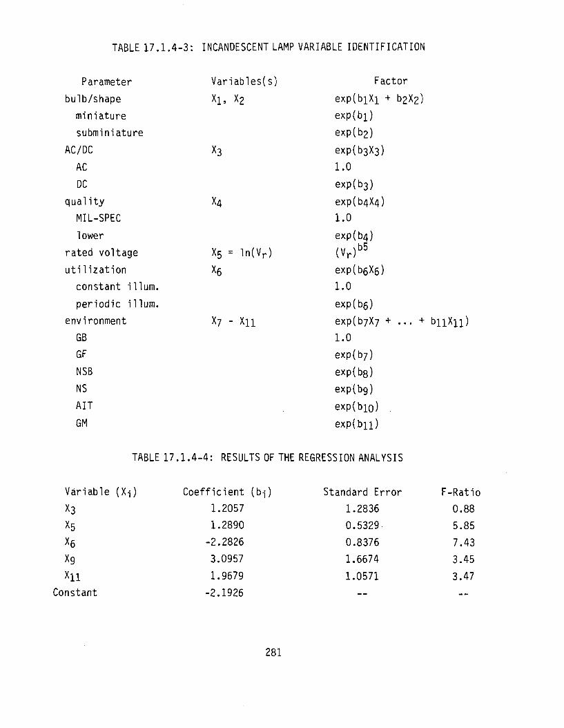
TABLE 17.1.4-3: INCANDESCENT LAMP VARIABLE IDENTIFICATION
Parameter
bulb/shape
miniature
subminiature
AC/DC
AC
DC
quality
MIL-SPEC
lower
rated voltage
utilization
constant ilium.
periodic ilium.
environment
6B 6F
NSB
NS
AIT
GM
Variables(s)
Xi, X2
X3
X4
X5 = ln(Vr)
X6
X7 - X n
Factor
exp(biXi + b2X2)
exp(bi)
exp(b2)
exp(b3X3)
1.0 exp(b3)
exp(b4X4)
1.0
exp(b4)
(V r)b 5
exp(b6X6)
1.0
exp(b6)
exp(b7X7 + ... +
1.0 exp(b7)
exp(b8)
exp'(bg)
exp(bio)
exp(bn)
bllXn)
TABLE 17.1.4-4: RESULTS OF THE REGRESSION ANALYSIS
Variable
X3 X5 X6 X9 Xll
Constant
(Xi) Coefficient
1.2057
1.2890
-2.2826
3.0957
1.9679
-2.1926
(bi) Standard Error
1.2836
0.5329
0.8376
1.6674
1.0571
__
F-Ratio
0.88
5.85
7.43
3.45
3.47
_ _
281

Strict interpretation of the results given in Table 17.1.4-4 were that
ground, benign; ground, fixed; naval, submarine and airborne inhabited,
bomber environments have a similar effect on lamp reliability and that naval,
sheltered (X-j^9=0, Xg=l) and ground, mobile (X-j f11=0» Xn=l) environments
adversely effect lamp reliability. For the number of available data records
and the anticipated "statistical noise", these results were not
discouraging. Only the inclusion of airborne inhabited, bomber with ground,
benign; ground, fixed and naval, submarine environment was considered
questionable. The anticipated relatively smaller numerical differences
between ground, benign; ground, fixed and naval, submarine environmental
factors could not be distinguished by regression analysis unless more data
records or more observed failures per data record were obtained.
Nevertheless, derivation of a complete set of environmental factors is
essential to properly discriminate against all incandescent lamp reliability
characteristics. No part type currently included in MIL-HDBK-217D
adequately represents the effects of environmental stress on lamps.
Therefore, the methodology described in Section 3.3 was applied to the
incandescent lamp data to derive an applicable series of environmental
factors. This method assumes that an environmental factor relation can be
determined where environmental factor is a function of the "environmental
stress ratios" given in Reference 1. Before application of this method, all
data was normalized by application, rated voltage and utilization.
Referring again to Tables 17.1.4-3 and 17.1.4-4, the normalization function
was obtained by the following progression of equations.
Ap = exp(b0) exp(b3X3) ( V r )b 5 exp(b6X6) irE
y(exp(b 3X 3) (V r )b 5 exp(b6X6)) = exp(bo) *E
Xp, norm = Xp/(exp(b3X3) ( V r )b 5 exp(b6X6))
282

Xp, norm = exp(b0) E
where
Xp = incandescent lamp failure rate
TT£ = environmental factor
Xp, norm = normalized failure rate
Various relations of normalized failure rate as a function of
environmental stress ratio were attempted. The optimal relation and the
corresponding environmental factor equation are given by,
Xp, norm = 0.0735 ( S ) 0 , 4 9 5
TfE = ( S ) 0 ' 4 9 5 , (normalized to TTE,GB = 1)
where
S = environmental stress ratio
The series of environmental factors obtained by this method were given in
Table 17.1.3-2 in the previous section. A result of normalizing the
environmental factors to a value of one for a ground, benign environment was
that refinement of the regression constant was necessary. The previously
determined regression constant (exp(b0) = exp(-2.19) = 0.112) represented an
average value for the ground, benign; ground, fixed; naval, submarine and
airborne inhabited, transport environments. The revised value (exp(b0) =
0.075) obtained from the environmental factor derivation process corresponds
to the ground, benign environment.
The derived environmental factors based on the data are lower than those
included in MIL-HDBK-217D for electronic parts. One explanation for this is
that operating temperature and temperature cycling theoretically have very
little effect on lamp life. The internal lamp illumination temperatures are
283

so high that elevated environmental temperatures and/or temperature cycling
are essentially negligible in comparison. Therefore the derived
incandescent lamp environmental factors are primarily a function of the
other two primary failure activating stresses, shock and vibration.
The regression analysis identified the rated voltage as a significant
variable effecting failure rate. The model indicates that failure rate is
proportional to rated voltage raised by an exponent equal to 1.289. The
rated voltage is a construction parameter which is the same for a particular
lamp regardless of the application. Therefore, it was decided to include the
rated voltage into a base failure rate relation. The base failure rate is
therefore a function of the rated voltage and is given by,
Xb = 0.074 ( V r )1 , 2 9
where
Xb = base failure rate (failures/10^ hours)
Vr = rated voltage (volts)
Applied voltage would also be anticipated to have a significant effect on
lamp reliability. Consideration of this factor is discussed in the following
paragraph.
All data collected in support of this study had an applied-to-rated
voltage ratio either equal to one or unknown and assummed equal to one. This
is not unusual because most design engineers do not "derate" lamp voltage.
However, it has been documented that incandescent lamp failure rate in AC
operation can be decreased by decreasing the applied voltage. References 2,
3, 5 and 6 include theoretical relations or examples of lamp life as a
function of applied to rated voltage. An example of a theoretical relation
between lamp life and applied to rated voltage is given below. This example
is from Reference 6.
284
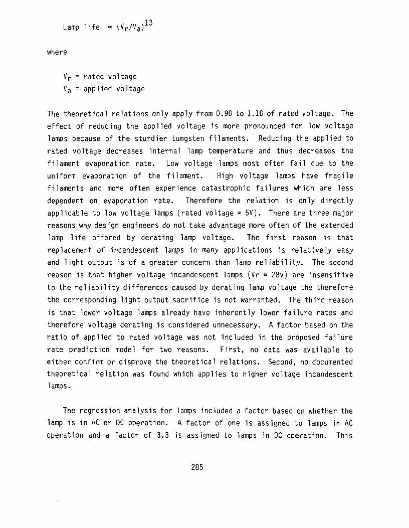
Lamp life « ^ V r / V a )1 0
where
Vr = rated voltage
Va = applied voltage
The theoretical relations only apply from 0.90 to 1.10 of rated voltage. The
effect of reducing the applied voltage is more pronounced for low voltage
lamps because of the sturdier tungsten filaments. Reducing the applied to
rated voltage decreases internal lamp temperature and thus decreases the
filament evaporation rate. Low voltage lamps most often fail due to the
uniform evaporation of the filament. High voltage lamps have fragile
filaments and more often experience catastrophic failures which are less
dependent on evaporation rate. Therefore the relation is only directly
applicable to low voltage lamps (rated voltage = 5V). There are three major
reasons why design engineers do not take advantage more often of the extended
lamp life offered by derating lamp voltage. The first reason is that
replacement of incandescent lamps in many applications is relatively easy
and light output is of a greater concern than lamp reliability. The second
reason is that higher voltage incandescent lamps (Vr - 28v) are insensitive
to the reliability differences caused by derating lamp voltage the therefore
the corresponding light output sacrifice is not warranted. The third reason
is that lower voltage lamps already have inherently lower failure rates and
therefore voltage derating is considered unnecessary. A factor based on the
ratio of applied to rated voltage was not included in the proposed failure
rate prediction model for two reasons. First, no data was available to
either confirm or disprove the theoretical relations. Second, no documented
theoretical relation was found which applies to higher voltage incandescent
lamps.
The regression analysis for lamps included a factor based on whether the
lamp is in AC or DC operation. A factor of one is assigned to lamps in AC
operation and a factor of 3.3 is assigned to lamps in DC operation. This
285

factor was designated the application factor. These results are consistent
with documented studies. Reference 2 states that "AC operation can increase
lamp life from two to ten times the life obtainable with DC operation."
Reference 3 states that "the life of an incandescent lamp energized by DC is
40 to 50% of life at the same voltage AC." Reference 4 found that "average
life of filaments operating on DC at the designed voltage is less than one-
third of that on AC." The observed failure rate ratio of 3.3 was based
solely on the empirical data given in Table 17.1.4-1.
The utilization of an incandescent lamp was thought to be a significant
factor in a failure rate prediction model. The results of the regression
analysis indicate an order of magnitude difference between applications
requiring constant illumination and those requiring periodic illumination.
The effect which utilization has on failure rate was represented by a
utilization factor (TTU). The numerical results are in complete agreement
with theoretical reliablity considerations. However, sufficient data were
available only for constant illumination, power indicator, warning indicator
and test light applications. These applications represent the two extreme
cases. Constant illuminati-on and power indicator lamps are illuminating
(and thus the filament is evaporating) for the entire time the equipment is
in use. Warning indicator lamps and test lamps are usually not illuminating
for the vast majority of the equipment operating time. Test lamps are
generally activated briefly at the start and the end of a mission and
accumulate very few illumination hours. Warning indicator lamps are
intended to illuminate very rarely. The duty cycle of a warning indicator is
very hard to predict but can be assumed to less than 10%. It should be noted
that life limiting stresses occur while lamps are in both illumination and
nonillumination modes. The problem with the regression solution is that
status indicator lamps or other lamp applications with variable duty cycles
were not included in the analysis. The one data record (entry #19, Table
17.1.4-1) where the lamp functioned as a status indicator has zero observed
failures. The lack of precision in estimating a failure rate without
observed failures is the reason that derivation of a numerical utilization
factor value for status indicators was difficult. However, an important
286

attribute of all reliability modeling efforts is to produce a usable model
which can be applied to all potential applications.
It was hypothesized that a continuous numerical relationship for
utilization factor as a function of lamp duty cycle would not be linear. The
hypothesized function was that the utilization factor would be relatively
close to the duty cycle for low (<0.10) and high (>0.90) duty cycles, but
would be higher than the duty cycle for intermediate duty cycle values. The
hypothesized relationship for utilization factor as a function of duty cycle
is presented in Figure 17.1.4-1. The reason for the hypothesized
nonlinearity shown in Figure 17.1.4-1 is the anticipated effect of "on-off"
power cycling. Applications with high and low duty cycles are subjected to
relatively fewer on-off cycles and the observed failure rate is primarily a
function of filament evaporation. Status indicator lamps with intermediate
duty cycles are subjected to more on-off cycles and the failure rate is a
function of both filament evaporation and on-off cycling. The amount of "on-
off" cycling for low, intermediate and high duty cycles is illustrated in
Figure 17.1.4-2. Based on the hypothesized relation, it was assumed that a
proposed utilization factor for status indicators would fall between the
value derived from constant illumination applications (1.0) and the
arithmetic mean of the values derived from constant illumination and warning
indicator applications (0.55). To determine a specific numerical quantity,
upper confidence limit failure rates were calculated for data entry number
19. The upper 80% confidence limit satisfied the boundary limits assumed for
a status indicator utilization factor. Therefore, the data was normalized
and a utilization factor of 0.72 was calculated by the following equation. A
discussion of Chi-squared confidence interval estimation is included in
section 3.1.
^u.s = X^80/(2T Xb irE TTA)
where
^UjS = utilization factor for status indicators
287

IX. o t— o
FIGURE 17.1.4-1: UTILIZATION FACTOR VS. DUTY CYCLE
DUTY CYCLE POWER
LAMP, LOW
LAMP, MEDIUM
LAMP, HIGH
EQUIPMENT _
FIGURE 17.1.4-2: LAMP VS. EQUIPMENT POWER FOR VARIOUS DUTY CYCLES
288
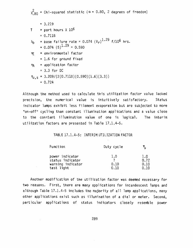
X 80 = Chl'-scluarecl statistic (a = 0.80, 2 degrees of freedom)
= 3.219
T = part hours X 10^
= 0.7118
*b = base failure rate = 0.074 ( V r )1 , 2 9 f/106 hrs.
= 0.074 ( 5 ) 1 , 2 9 = 0.590
TIE = environmental factor
= 1.6 for ground fixed
TT/\ = application factor
= 3.3 for DC
TTU5S = 3.209/(2(0.7118)(0.590)(1.6)(3.3))
= 0.724
Although the method used to calculate this utilization factor value lacked
precision, the numerical value is intuitively satisfactory. Status
indicator lamps exhibit less filament evaporation but are subjected to more
"on-off" cycling than constant illumination applications and a value close
to the constant illumination value of one is logical. The interim
utilization factors are presented in Table 17.1.4-5.
TABLE 17.1.4-5: INTERIM UTILIZATION FACTOR
Function Duty cycle \
power indicator 1.0 1.0 status indicator ? 0.72 warning indicator 0.10 0.10 test light 0.10 0.10
Another modification of the utilization factor was deemed necessary for
two reasons. First, there are many applications for incandescent lamps and
although Table 17.1.4-5 includes the majority of all lamp applications, many
other applications exist such as illumination of a dial or meter. Second,
particular applications of status indicators closely resemble power
289

indicator (constant illumination and little "on-off" cycling) or warning
indicator (little or no illumination) and therefore should be assigned the
more appropriate utilization factor value. Therefore a final utilization
factor was determined and three general utilization types were defined and
are presented in Table 17.1.4-6.
TABLE 17.1.4-6: UTILIZATION FACTOR
Utilization type Illuminate hours/ 7ru equipment operate hrs.
A > 0.90 1.0 B 0.10 to 0.90 0.72 C < 0.10 0.10
The boundaries of the B category were chosen so that most applications
would fall immediately into one category or another and that a specific
numerical quantity of (illuminate hours/equipment hours) would not be
required of the analyst preforming the reliability prediction. It should be
noted that the three choices given in Table 17.1.4-5 represent three unique
applications and that no attempt should be made to interpolate between the
numerical values.
The effect of "on-off" cycling is not included directly in the proposed
failure rate prediction model. However, the model accounts for "on-off"
cycling two different ways. Missions within an environment category are
similar in regard to mission duration. For example the typical helicopter
mission would be expected to be much shorter than the typical mission in a
ground fixed environment. Therefore the higher frequency of on-off cycles
generally would occur in the helicoptor environment. Therefore the effect of
on-off cycling is included in the environmental factor to the extent that the
average frequency of on-off cycling is different between environment
categories. The effect of on-off cycling is also included partially in the
proposed utilization factor. For a particular environment category the
relative frequency of on-off cycling is low for applications with both high
290
and low duty cycles (utilization types A and C in Table 17.1.4-5) and
relatively higher for applications with an intermediate duty cycle.
The proposed failure rate prediction model offers greater sensitivity to
incandescent lamp reliability characteristics. The existing MIL-HDBK-217D
methodology for prediction of lamp failure rate was a point estimate failure
rate for all lamp applications. The proposed model presents incandescent
lamp failure rate as a function of rated voltage, environment, utilization
and application. The proposed model offers the reliability analyst a more
accurate and precise measure of lamp reliability and it is recommended that
the proposed model be included in the latest revision of MIL-HDBK-217.
17.1.5 References and Bibliography
References
1. Kremp, B.F. and E.W. Kimball, Revision of Environmental Factors for MIL-HDBK-217B, RADC-TR-80-299, September 1980.
2. Sylvania Miniature Lightings Products, Properties of Miniature Lamps, Machine Design, Vol. 46, No. 30, Dec. 12, 1974.
3. Dombroski, C , Indicator Lamps - The Sooner the Brighter, Electronic Products, April 1978.
4. Koo, R.C. and J. Woodhouse, Observations on Electromigration and Improved Filament Life of Microminiature Lamps, Journal of the Society of Illuminating Engineers, Vol. 5, July 1976.
5. Chicago Miniature Lamp Works, Lamp Comparison and Evaluation of the Industry Standards No. 327 and No. 387 Subminiature Lamps.
6. Fink, D.6. and D. Christiansen, Electronics Engineer's Handbook, Second Edition, Section 11, McGraw-Hill Book Co., 1982.
Bibliography
Dawson, C.W., Nelson, J.L., et. al., Hot Spots and Their Effect on The Lives of Incandescent Filaments, Journal of the Society of Illuminating Engineers, July 1973.
Horacsek, 0., Properties and Failure Modes of Incandescent Tungsten Filaments, IEE Proceedings, Vol. 127, Pt. A, No. 3, April 1980.
291
17.2 Lamps, Glow
17.2.1 Part Description
The following discussion was extracted primarily from reference 1. The
glow lamp is basically a negative discharge device. It consists of two
closely spaced electrodes housed in a glass envelope filled with rare gas
(neon, argon, etc.). When a sufficient amount of voltage is applied across
the terminals of a glow lamp, it exhibits what are called breakdown
characteristics; that is, the gas ionizes and the voltage across the lamp
drops very quickly to a reduced level which is called its maintaining
voltage. When this condition occurs, there is the appearance of a glow
surrounding the negative electrode.
Glow lamps have properties that permit them to be used as light sources
or circuit components. As a light source, they permit a method of giving
high voltage (115 volts) illumination in a small envelope. They are
generally more rugged and more reliable than incandescent lamps.
Illumination efficiency of standard brightness units is quite low, about
0.005 candlepower per milliamp, while for high brightness units it is about
0.013 candlepower per milliamp. This gives a brightness of about 0.0035
candlepower for a typical standard brightness unit and about 0.025
candlepower for high brightness units. Therefore, these units are not nearly
as bright as typical incandescent lamps.
Glow lamps have many varied uses. In addition to being used as a lamp,
they often serve as circuit components. Some of their uses include:
indicator, voltage indicator, voltage regulator, low frequency generator,
and leakage detector. Glow lamps are subject to "runaway" conditions;
therefore, they must always be operated in series with a current limiting
device, such as a resistor.
Glow lamps exhibit excellent environmental resistance and much higher
vibration resistance than incandescent lamps. They should never be used
292

above 150°C and, in circuit applications, are not recommended above 75°C.
When glow lamps are subjected to darkened environments, their breakdown
voltage rises and ionization time increases. Lamps are available which
include use of mild radioactive additives to reduce their susceptibility to
darkened environments. Glow lamp operation is affected by electrostatic and
electromagnetic fields. It is possible to ignite a glow lamp in a strong
electromagnetic field with no applied voltage.
The definition of life differs with various glow types. Standard
brightness indicator types are said to reach end of life when their light
output decreases to 50% of initial. High brightness lamps remain essentially
constant in light output through life, and fail when breakdown voltage
reaches line voltage. Circuit component types reach end of life when their
starting or maintaining voltage changes some definite value (usually 5 or 10
volts) from initial rating. References 2 and 3 state that the average useful
life (time to 50% of initial output) for dc operation is 60% of the average
useful life for ac operation.
17.2.2 Failure Modes and Mechanisms
The primary failure modes for glow lamps are as follows:
o deterioration or destruction of the seal caused by defective materials and/or process, or handling problems. This will result in an open lamp because of the absence of a discharge between electrodes.
o open lead wire in the base of the lamp or on wire leaded lamps external to the base caused by poor workmanship or defective materials. This will result in an open or intermittent lamp.
o shorted lead wires in the base of the lamp caused by faulty workmanship. This will result in a shorted lamp with no light emission.
o excessive current flow through the lamp or excessive voltage across the lamp causes an arc to form between the electrodes. This will result in rapid lamp deterioration.
293

17.2.3 Glow Lamp Failure Rate Prediction Model
This section presents the proposed failure rate prediction model for
glow lamps. The proposed model is:
Xp = 0.2F/106 hours
The model is limited to neon glow lamps.
17.2.4 Model Development
The approach used was to hypothesize a model form based on physics of
failure information. The model form would be verified and parameters would
be quantified by analysis of data collected during the study. The model that
was assumed is:
Xp = Xb x TTE x Try x TTQ X TT/\
where
Xp = glow lamp failure rate (F/10^ hours)
Xb = base failure rate (F/10^ hours) and where Xb is a function of the
lamp type
TTE = environmental factor
TTJ = temperature factor
TTQ = quality factor
TTA = application factor
The rationale for including the factors given above is discussed in the
following paragraphs.
Glow lamps may contain argon, neon or a mixture of gases. The circuit
connection technique is either through a base or through lead wires. The
deterioration characteristics of the gases differ. For instance, the
294
average of the specified lives from references 4, 5, 6 is approximately
14,900 hours for neon and 150 hours for argon glow lamps. Since the two
connection techniques are so different it would be expected that their
failure characteristics would be different. For example, from references 4,
5 and 6, the average of the specified lives is approximately 16,300 hours for
wire lead devices and 21,100 hours for devices with a base. In addition, the
failure modes of standard brightness indicators and high brightness lamps
differ; therefore, the failure rate should differ. The construction of the
glow lamp probably is correlated with the expected life of the device. The
specified life of the devices varied from 7,500 to 100,000 hours for neon
indicator lamps and from 500 to 25,000 hours for neon circuit component
devices; however, the driving construction characteristic responsible for
these differences was not obvious from the data (references 4, 5 and 6). It
was assumed then that ^ would vary as a function of gas type, construction
basing mechanism and whether it is a standard or high brightness lamp.
Glow lamps behave differently in a darkened environment and in the
presence of electrostatic and electromagnetic fields. Since they behave
differently, it could be expected that their failure rate would differ
depending on the environment. It was assumed that an environmental factor
could be derived that would account for those differences in behavior.
Glow lamps have an upper temperature limit which should never be
exceeded, and they exhibit a negative temperature coefficient. In addition,
gas diffusion and bond strength are a function of temperature. These factors
would indicate that device failure rate may be a function of temperature.
Glow lamps are manufactured devices and as such are subject to
manufacturing deficiencies. In addition, glow lamps can be burned-in to
reduce the number of infant mortality failures and to stabilize the breakdown
and maintaining voltages. Failure rate then may be a function of
manufacturing quality and whether or not a burn-in was performed.
295
Glow lamps are used for numerous applications including voltage
detection, voltage regulation, low frequency generators and indicators. The
definition of failure should vary for the various applications. The average
of the specified lives from references 2, 3 and 4 is approximately 5,900
hours for circuit component neon lamps and 22,500 hours for neon indicator
lamps. Failure rate then may be a function of how the lamp is used in the
circuit.
Based on the above considerations, application and construction
variables were identified (Table 17.2-1). These application and
construction variables represent possible failure rate model parameters
which were determined whenever possible for all collected data.
The glow lamp failure experience data collected in support of this study
are presented in Table 17.2-2. As can be seen from the data, there is
insufficient data to develop parameters for the model form assumed above.
Also since all of the data are for the same basic lamp type used in the same
application there was insufficient data to disprove the current MIL-HDBK-
217D point failure rate estimate for neon lamps. It is proposed then that
the current MIL-HDBK-217D model be retained. The low failure rate of the
device and the fact that they are increasingly being replaced in circuit
applications by solid state voltage regulators, and solid state and liquid
crystal indicators may indicate that the current model is sufficient.
17.2.5 References and Bibliography
References
1. General Electric Company, Component Technology and Standardization Manual, Section 11.2.
2. Glowhite Product Catalog.
3. Xenell Corporation Product Catalog.
4. Herman H. Smith Product Catalog.
296

TABLE 17.2-1: GLOW LAMP CONSTRUCTION AND APPLICATION VARIABLES
I. Type A. Neon B. Argon C. Mixture
II. Bulb Shape A. Globular B. Straight Side C. Tubular D. Other
III. Mounting Method A. Base B. Lead
IV. Function A. Light Source B. Indicator C. Voltage Regulator D. Low Frequency Generator
V. Current Level A. Rated B. Actual
VI. Voltage Level A. Rated B. Actual
VII. Operating Temperature A. Rated B. Actual
VIII. Application Environment
IX. Manufacturing Quality Level
297

»— t-H rn
5 ffi O u"1
cr. co i n f—<
c\j o
CO
o
l/) — -i-«x>
X O
«£> « •
C\J
m C\J f - H
,_( o r^
m i n C\J
«£> i n
m
m CO O i
i n f - H
C\J
r^ r^ CO
.-H O
B <-> OJO
o
0) O) X I D. => >>
^* o ^ ^* ^*
=> > > cr l -
298

Bibliography
Arno, Robert G., Nonelectronic Parts Reliability Data, Reliability Analysis Center Document NPRD-2, Summer, 1981.
General Electric Company, Component Technology and Standardization Manual, Section 11.2.
Glowhite Product Catalog.
Herman H. Smith Product Catalog.
Xenell Corporation Product Catalog.
299

18.0 SURFACE ACOUSTIC WAVE DEVICES
18.1 Part Description
Surface Acoustic Wave (SAW) devices are any of a number of signal
processing devices which operate by converting an electrical signal to an
acoustic wave travelling along the surface of the medium. The surface
acoustic wave has both longitudinal (compressive) and transverse (shear)
components, and has the majority of its energy concentrated within one
acoustic wavelength of the surface within the bulk. SAW devices are finding
widespread use for a number of signal processing requirements at UHF and
microwave frequencies.
In its simplest form, a SAW device consists of a pair of electrical
conductors placed on each end of a piezoelectric crystal. When an electrical
potential energizes one conductor pair, the piezoelectric crystal will
mechanically distort, creating a surface wave which is transmitted through
the crystal at a velocity dependant upon the material properties of the
device. At the other end, the second pair of conductors detect the surface
wave and outputs a corresponding electrical signal to the circuit. The
velocity of a SAW is on the order of 10~5 that of electric field propagation
in free space, making them useful as delay lines in electrical circuits.
By the addition of simple electrodes to otherwise standard piezoelectric
delay lines, it is possible to use these delay lines to generate the
convolution and correlation functions of an unknown signal with an arbitrary
reference signal. By suitable choice of a reference signal, pulse
compression and other signal processing operations may be performed.
Electrodes are usually fabricated in the form of an interdigitated
structure as in Figure 18.1-1. The response of a SAW device may be
controlled by altering the finger position width and amount of overlap.
300
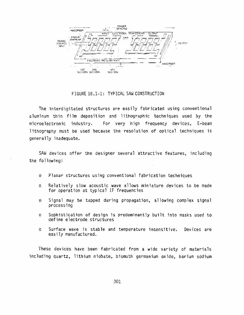
FINGER - - . L * " " SPACING
•• ABSORBER >- * " "
S.GNAI ; O V E R L A P
/ _ INPUT ELECTRODE TRANSDUCER OUTPUT ,_,
FINGER*\ / | Q^~ ~~ "~ *
/{" / / " -Jt=i' ' (=!=•• /••'' Ui i
PIEZOELE^ffRIC~SlJBSTRATE
1 ST 2ND NTH SECTION SECTION SECTION
FIGURE 18.1-1: TYPICAL SAW CONSTRUCTION
The interdigitated structures are easily fabricated using conventional
aluminum thin film deposition and lithographic techniques used by the
microelectronic industry. For \jery high frequency devices, E-beam
lithography must be used because the resolution of optical techniques is
generally inadequate.
SAW devices offer the designer several attractive features, including
the following:
o Planar structures using conventional fabrication techniques
o Relatively slow acoustic wave allows miniature devices to be made for operation at typical IF frequencies
o Signal may be tapped during propagation, allowing complex signal processing
o Sophistication of design is predominantly built into masks used to define electrode structures
o Surface wave is stable and temperature insensitive. Devices are easily manufactured.
These devices have been fabricated from a wide variety of materials
including quartz, lithium niobate, bismuth germanium oxide, barium sodium
301

niobate, cadmium sulfide, diamond, europium iron garnet, gallium arsenide,
and many others.
The simplicity and versatility of surface acoustic wave devices makes
them desirable for a number of high reliability state-of-the-art military
systems including radar, communication, sonar, air traffic control, and
display systems. Specific uses for SAW devices include delay lines,
frequency filters, oscillators, matched filters, code generators,
convolvers, and IF signal processing applications.
18.2 Failure Modes and Mechanisms
While the relative simplicity of these devices makes them reliable in a
wide variety of applications, there are several failure modes and mechanisms
to which these devices are susceptible. As their name might suggest, surface
acoustic wave devices are susceptible to degradation as a result of surface
contamination. It is important that the surface of high frequency devices be
kept scrupulously clean. Small amounts of organic material can cause a large
amount of surface wave attenuation.
Strain effects are very important in SAW devices. Unintentional strain
results in devices with highly variable properties. This requires that
particular care be exercised when bonding a SAW device to a substrate, so
that no residual strain is present after the bonding operation. Also, if the
operating temperature is to vary widely in use, it is important that thermal
expansion rates for the SAW device and substrate be carefully matched.
Due to the extremely small finger dimensions on high frequency devices,
the SAW component is very sensitive to electrostatic discharge (ESD) damage
(at voltages as low as 150 volts on piezoelectric quartz and lithium
niobate). ESD damage may manifest itself as a melting of interdigitated
metal runs, a fracturing of the crystal surface, or both. As a consequence,
it is imperative that SAW devices be manufactured, handled, and used in
conditions where ESD protective measures have been implemented.
302

In addition to the above mentioned conditions, the surface wave device is
vulnerable to the usual problems of crystal growth, thin film deposition, and
lithographic defects, and packaging problems which are well documented in
semiconductor and hybrid reliability studies. Table 18.2-1 lists the
failure modes/mechanisms that have been either reported in the published
literature or recorded with the data collected during the study.
TABLE 18.2-1: REPORTED FAILURE MODES/MECHANISMS
Source Number of Occurences*
Failure Mode/Mechanism
5
6
Wire bond failure.
Open ground wire connection.
Cracks in substrate during manufacture caused by rapid temperature change.
Polyimide used to bond SAW devices. If insufficient polyimide is used, it will tend to crack, effectively demounting the SAW.
Aluminum migration induced acoustic fields.
by high density
Growth of aluminum oxide on the thin film aluminum metal induced by water vapor and a dc electric field within the transducer structure (Ref. 1).
Short fused (open) regions and melting of fingers and arc discharge regions across fingers induced by dc voltage transients as low as 150 volts (Ref. 2).
*'-' indicates, that the number of occurences was not reported,
303

18.3 SAW Failure Rate Prediction Model
This section presents the proposed failure rate prediction model for
Surface Acoustic Wave Devices. The proposed model is:
Xp = Xb x TTE
where
Xp = predicted SAW failure rate (F/106 hours)
Xb = base failure rate
= 2.1 F/106 hours
•HE = environmental factor (see Table 18.3-1)
TABLE 18.3-1: ENVIRONMENTAL FACTORS
Environment
GB
GF
GM Mp
NSB NS Nu NH
NUU ARW
AlC AIT
AlB
E 1.0
3.9
11.0
10.0
4.95
8.5
16.0
15.5
17.0
22.5
7.5
7.5 12.5
Environment
AlA
AlF
AlIC
AUT
AUB AUA
AUF
SF MFF MFA
USL ML
CL
E 10.0
15.0
12.5
10.0
20.0
15.0
20.0
1.6
10.5
14.5
30.5
35.0
600.0
18.4 Failure Rate Model Development
The model development approach used was to assume a model of the form:
Xp = Xb ITE- A base failure rate (Xb) estimate was then derived from the
304

observed data shown in Table 18.4-1. A failure rate prediction model of this
form oversimplifies the reliability characteristics of SAW devices.
However, the lack of available field failure rate data and the unavailability
of data from SAW manufacturers necessitated this model format.
TABLE 18.4-1: SAW FAILURE EXPERIENCE DATA
Source (Note 1)
1 2 8 9
Totals
Env
AlC GB SF GF
No. Fail.
1 1 0 0 2
Sample Size
32
46
Operate Hours (X106)
0.062 0.691 0.788 0.036 1.577
Failure Rate (F/1 L10%CL PI EST
(Note 2)
1.70 16.10 0.15 1.45
1.17 25.68
0° hou U90%C
62.64 5.63 2.92
64.21
Notes:
1) Source 1: WIDE and Narrow Band Expanders and Compressors, equipment type unknown Source 2 Source 8 Source 9
1393 MHZ Oscillator, life test data Device Function unknown, equipment type unknown Elastic Convolver, equipment type unknown
2) Upper 60% confidence limit for zero failure data
Because of the construction and reported failure mode/mechanism
similarities between SAW and hybrid devices and because the acquired data
were too sparse to develop environmental factors directly from the data, the
environmental factors for hybrid device resistors, interconnections and
packages presented in reference 1 were examined to determine their
applicability for the SAW model. The ratio of the failure rates from the
four data points were compared with the ratio of the environmental factors
presented in reference 3 for hybrid device resistors, interconnections and
packages. These data are shown in Table 18.4-2.
305

TABLE 18.4-2: ENVIRONMENTAL COMPARISONS
Env
GB SF GF AIC
MIL-HDBK-217 TTE Ratio
1.0 1.6 3.9 7.5
Upper 60% CL Failure Rate Ratio of (F/106 hours) observed
failure rates
2.9 1.0 1.2 0.4
25.7 8.9 32.6 11.6
With the exception of the space flight environment factor, the progression of
the observed factors track the progression of the current MIL-HDBK-217
factors for hybrids. One possible explanation for the space flight
discrepancy is that the zero failures observed for the space flight data was
an assumption made by the source of the data because the equipment was still
operational. With the level of redundancy built into the equipment, this
could be an optimistic assumption. Based on results shown above and the
limited amount of data available (4 points and 2 failures), there is no
reason to reject the assumption that the environmental factors presented in
reference 3 for hybrids can be used to predict the failure rate of SAW
devices.
The MIL-HDBK-217 HE ratios given above were then used to normalize the
data to the ground benign environment. The normalized data including point
estimate failure rates, lower 10%, upper 60%, and upper 90% confidence limits
are presented in Table 18.4-3.
TABLE 18.4-3: NORMALIZED FAILURE DATA
Source No Env Actual Normalized Normalized Failure Rate (F/106 hours) Fail OPHRS OPHRS L10%CL PT EST U60%CL U90%CL
(X106) (X106)
1 2 8 9
Total
1 1 0 0 2
AlC GB SF GF
0.062 0.691 0.788 0.036
-
0.466 0.691 1.261 0.140 2.558
0.23 0.15
--
0.21
2.15 1.45
--
0.78
4.35 2.93 0.73 6.58 1.21
8.35 5.63 1.83
16.46 2.08
306

It was then determined that the optimal base failure rate for SAWs was the
90% upper confidence level estimate of 2.08F/106 hours. It was decided to
apply this somewhat pessimistic value for base failure rate because of the
relative scarcity of available data and the lack of discrimination in the
proposed model against construction and usage variables. This estimate was
rounded to two significant digits for inclusion in the handbook. The
environmental factors presented in reference 3 for hybrid devices were then
normalized to a ground benign value of 1.0 (see Table 18.3-1). A graph of
the predicted to observed failure rates listed in Table 18.4-1 is shown in
Figure 18.4-1. The upper 90% and lower 10% confidence limits are also shown
on the graph.
18.5 References and Bibliography
References
1. Allen, Donald E., et. al., A Latent Failure Mechanism for Surface Acoustic Wave Components Utilizing Lithium Niobate, 18th Annual Reliability Physics Symposium, 1980.
2. Hickernell, F.S., DC Voltage Effects On SAW Device Interdigital Electrodes, J.8th Annual Reliability Physics Symposium, 1980".
iff 7 7
3. Edwards, E., et. al., Avionic Environmental Factors for MIL-HDBK-217, Final Technical Report, RADC-TR-81-374, January, 1982.
Bibliography
Allen, Donald E., et. al., A Latent Failure Mechanism for Surface Acoustic Wave Components Utilizing Lithium Niobate, 18th Annual Reliability Physics Symposium, 1980.
Annon., SAW Upsurge Likely in Avionics, Defense Electronics, February, 1981, p. 37.
Edwards, E., et. al., Avionic Environmental Factors For MIL-HDBK-217, Final Technical Report, RADC-TR-81-374, January, 1982.
Feinstein, Joseph, Passive Microwave Components, Electronics Engineers Handbook, Second Edition, McGraw-Hill, 1982.
307

500
200
100
50
20
10
/
/ 1
\ '
>
/
< •
/
.1 .2 .5 1 10 20 50 100
PREDICTED FAILURE RATE (F/106 hours)
FIGURE 18.4-1: PREDICTED VS OBSERVED FAILURE RATES
308

Hickernell, F.S., DC Voltage Effects On SAW Device Interdigital Electrodes, 18th Annual Reliability Physics Symposium, 1980.
Hughes Aircraft Company, 2nd Quarterly Report, Contract No. N00014-81-C-2356, Broadband IOSA SAW Transducer Study, January, 1982.
Levine, B., SAW Technology Applications Probed, Source Annon.
Martin Marietta Corporation, Reliability Prediction Models for Microwave Solid State Devices, RADC-TR-79-50, April, 1979.
Murray, R.J., and White, P.D., SAW components answer today's signal-processing needs, Electronics, Vol. 54, September 8, 1981, pp. 120 - 124.
Reeder, T.M. et. al., Frequency Output Pressure Sensors Based on an Application of Surface Acoustic Wave Technology, Society of Automotive Engineers pamplet No. 760093.
Reible, Stanley A., Acoustoelectric Convolver Technology for Spread-Spectrum Communications, IEEE Transactions on Microwave Theory and Techniques, Vol. MTT-29, No. 5, May, 1981, pp. 463-473.
Shoquist, Tom, Sink Your Teeth Into a SAW, Electronic Products, May 1979, pp. 63-66.
Shreve, W.R., et. al., Power Dependence of Aging in SAW Resonators, preprint to be published in 1981 Ultrasonics Symposium Proceedings.
Yao, I. and Reible, S.A., Wide Bandwidth Acoustoelectric Convolvers, Ultrasonics Symposium Proceedings, September, 1979.
309

19.0 CONCLUSIONS AND RECOMMENDATIONS
19.1 Conclusions
Failure rate prediction procedures were developed for the following
devices:
o Vidicons o Semiconductor Lasers o Helium-Cadmium Lasers o Electronic Filters o Solid State Relays o I.C. Sockets o Thumbwheel Switches o Surface Acoustic Wave Devices
In addition, the prediction procedures for the following devices were
revised:
o Magnetrons o Electronic Time Delay Relays o Circuit Breakers o Meters o Fuses o Crystals o Incandescent Lamps o Cathode Ray Tubes
Both the new and the revised failure rate prediction procedures will greatly
improve upon current failure rate prediction capabilities. The advantages
offered by the proposed failure rate prediction procedures are discussed in
the following paragraph.
Previously no single acceptable source of failure rates was available
for the first group of devices given above. Their inclusion into MIL-HDBK-
217 will allow for more consistent evaluations of reliability predictions,
reliability trade-offs and life-cycle cost analyses. The revision of the
failure rate prediction procedures for the second group of devices listed
310

above will provide greater sensitivity and increased accuracy in the
predictions.
The failure rate prediction procedures for the following devices could
not be revised:
o Helium-Neon Lasers o Solid State Rod Lasers o CO2 Lasers 0 Argon Ion Lasers 0 Neon Glow Lamps
With the exception of Nd:YAG solid state lasers and neon glow lamps, these
devices are not used to any great extent in military systems; consequently
very little field failure experience data are available. The Nd:YAG laser is
used in a number of military equipments; however, data were only available on
three of these systems. This amount of data was insufficient to allow for
the revision of the current model. Neon glow lamps are used sporadically
throughout military equipments. Data were obtained from five military
equipments; however, this amount of data was insufficient to allow for the
revision of the current model. The low failure rate of this device and the
fact that it is increasingly being replaced by solid state voltage regulators
and both solid state and liquid crystal indicators would indicate that the
current model is adequate.
None of the part failure rate models developed or revised during this
study effort are as sophisticated as was originally intended. This was
entirely due to lack of sufficient data or lack of detail in the data. The
reasons for these data deficiencies are:
0 Part types not normally used in military systems (e.g., Argon Ion, CO2, Helium Neon and Helium Cadmium lasers).
0 Part types are low population devices (e.g., neon lamps, SAWs).
0 Data contributors are generally reluctant to incur any expenditure to further refine data and information they provide without charge.
311

o Part failures are hard to define (e.g. fuses, circuit breakers).
o Potential data contributors are hesitant to allow visitors access to their proprietary databases.
Consequently, many of the factors considered could not be included in the
proposed models. Additionally, many of the factors that were included in the
proposed models had to be developed from existing MIL-HDBK-217 models for
similar devices, or had to be developed by other analytical methods and not
directly from field experience data.
19.2 Recommendations
It is recommended that both the proposed new models developed during this
study and the proposed revised versions of existing models be incorporated
into MIL-HDBK-217.
Although the proposed failure rate prediction procedures greatly improve
prediction capabilities, several recommendations are necessary in light of
all available information. All of the devices studied could be classified as
low population parts; consequently, most of the proposed models were based on
limited data resources. Only a few of the devices do not exhibit
sufficiently high failure rates and/or are not used in sufficient quantity to
have a noticeable impact on predicted equipment reliability. These devices
are:
o Neon Glow Lamps o Incandescent Lamps o Fuses o Crystals o I.C. Sockets
The failure rate of any of the remaining devices may constitute a large
portion of the total predicted equipment reliability; therefore, the
respective failure rate prediction models should be investigated further to
enhance their accuracy and sensitivity.
312

Several of the device types that were studied, including lasers and
surface acoustic wave devices, could be considered emerging technologies.
New lasing mediums are being introduced such as the blue-green Xenon-
Chloride (XeCl) and Mercurous-Bromide (HgBr) lasers, and new techniques such
as high pressure sealed CW CO2 lasers. These types of lasers are currently
not considered in MIL-HDBK-217. In addition, factors which are thought to
impact laser reliability such as optical power density, tube power output,
and incorporation of a simmer circuit in the solid state laser power supply
are not currently considered in MIL-HDBK-217. Surface acoustic wave devices
perform many functions (e.g., filter, delay, amplify, etc.) and can assume
various levels of complexity. The proposed model does not address these
factors which are thought to impact reliability. Every possible attempt
should be made in the future to collect field failure rate data so that the
failure rate prediction capability for these devices can be enhanced.
Analyses of the data and published information on many of the mature
devices disclosed factors which were thought to impact the reliability of the
device, but which either could not be investigated due to lack of data (e.g.,
focusing method on CRTs, environment on semiconductor lasers, etc.) or which
could not be confirmed because of insufficient data (e.g., deflection method
on CRTs, number of guns on CRTs, etc.). Every effort should be made to
collect field failure rate data on these devices so that greater sensitivity
and accuracy can be incorporated into their prediction procedures.
Air Force Regulation AFR 800-18 states: "to insure that every Air Force
system is available for use when needed, will perform its assigned missions,
and can be operated and supported economically, it is necessary to use and
support GIDEP and the DoD Reliability Analysis Center." The following clause
should be added to this statement: "and if data are to be available in
sufficient quantities to provide support for reliability studies." The
government provides funds for many maintenance support, life-cycle cost and
reliability improvement warranty contracts which yield meaningful field
failure experience data. A centralized point such as GIDEP or the
Reliability Analysis Center should be on automatic distribution to receive
313
copies of the raw data collected during these contracts. These data would
then be available for use in reliability studies such as the Reliability
Modeling of Critical Electronic Devices effort.
It was noted during this study that many of the part and equipment
manufacturers were reluctant to furnish uncontracted data free of charge.
This reluctance may be due to material and manpower costs incurred in
providing the data, or due to the proprietary nature of the data. The study
contractor is normally not provided with sufficient funds to allow for the
purchase of these data. The government should investigate methods of
identifying when reliability data are generated, of analyzing the merits of
the data, of providing a method of purchasing the data and of storing the
data in a central repository which is available to all government
contractors.
The proposed models for the non-mature devices (e.g., lasers, SAWs)
should be updated and revised periodically, i.e., every three to five years.
This would allow for changes in the state-of-the-art to be included on a
timely basis.
314
Appendix A
Proposed Revision Pages
For
MIL-HDBK-217
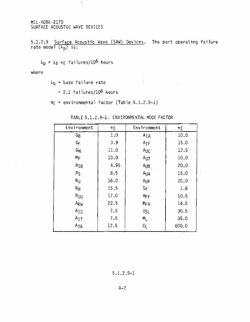
MIL-HDBK-217D SURFACE ACOUSTIC WAVE DEVICES
5.1.2.9 Surface Acoustic Wave (SAW) Devices. The part operating failure rate model (Xp) is:
^p = ^b ^E failures/106 hours
where
Xb = base failure rate
= 2.1 failures/106 hours
TT£ = environmental factor (Table 5.1.2.9-1)
TABLE 5.1.2.9-1. ENVIRONMENTAL MODE FACTOR
Environment
SB
6F GM Mp
NSB Ns
Nu NH NUU ARW
AlC AIT
AlB
TTE
1.0 3.9
11.0
10.0
4.95
8.5
16.0
15.5
17.0
22.5
7.5 7.5
12.5
Environment
AlA
AlF
AUC AUT
ALIB
AUA
AUF
SF MFF
MFA
USL ML
CL
TTE
10.0
15.0
12.5
10.0
20.0
15.0
20.0
1.6 10.5
14.5
30.5
35.0
600.0
5.1.2.9-1

MIL-HDBK-217D SEMICONDUCTOR LASER DEVICES
5.1.3.11 Semiconductor Laser Devices
SPECIFICATION DESCRIPTION
None Aluminum gallium arsenide (AlGaAs), Double Hetero-junction (DH), Stripe-geometry, Proton-isolated or Oxide-isolated structure
None Gallium Arsenide (GaAs), Single Heterojunction (SH), Stripe-geometry, Proton-isolated or Oxide-isolated structure
None Indium gallium arsenide/Indium gallium arsenide phosphorus (InGaAs/InGaAsP), DH, Stripe-geometry, Proton-isolated or Oxide-isolated structures
The part failure rate model Xp is:
Xp = Xb iTE
where
X p = total device.failure rate (F/106 hours)
Xb = average failure rate (F/106 hours)
iTE = environmental factor (Table 5.1.3.11-1)
The failure rate prediction procedure is as follows:
Step 1: Calculate the average failure rate (Xb)
Step 1A: Calculate the average optical power output degradation rate using the following equation:
TP = T b ITT 7TI TTC 7TA 7TF
where
Tp = semiconductor laser optical power output degradation rate (%/1000 hours)
xb = base degradation rate (56/1000 hours) (Table 5.1.3.11-2)
A-3
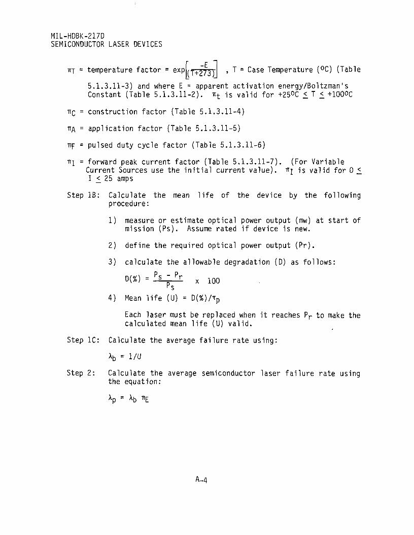
MIL-HDBK-217D SEMICONDUCTOR LASER DEVICES
•wj = temperature factor = exp (T+273~T ' T = ^ase T e m P e r a t u r e (°C) (Table
5.1.3.11-3) and where E = apparent activation energy/Boltzman's Constant (Table 5.1.3.11-2). irt is valid for +25°C < T < +100OC
TTQ = construction factor (Table 5.1.3.11-4)
TTA = application factor (Table 5.1.3.11-5)
Trp = pulsed duty cycle factor (Table 5.1.3.11-6)
Tq = forward peak current factor (Table 5.1.3.11-7). (For Variable Current Sources use the initial current value), ifj is valid for 0 £ I £ 25 amps
Step IB: Calculate the mean life of the device by the following procedure:
1) measure or estimate optical power output (mw) at start of mission (Ps). Assume rated if device is new.
2) define the required optical power output (Pr).
3) calculate the allowable degradation (D) as follows:
D(X) = fs_z_Pr x 1Q0 *s
4) Mean life (U) = D(%)/xp
Each laser must be replaced when it reaches Pr to make the calculated mean life (U) valid.
Step 1C: Calculate the average failure rate using:
Xb = 1/U
Step 2: Calculate the average semiconductor laser failure rate using the equation:
Xp = Xb TTE
A-4
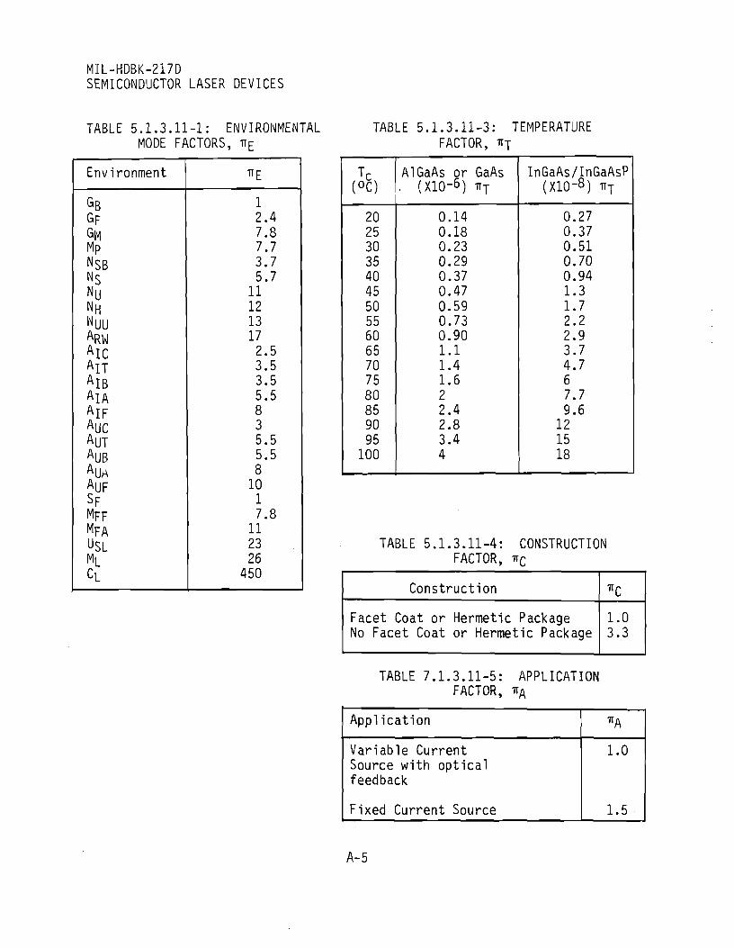
MIL-HDBK-217D SEMICONDUCTOR LASER DEVICES
TABLE 5.1.3.11-1: ENVIRONMENTAL MODE FACTORS, TTE
Environment
sB GF GM Mp NSB NS Ny NH NUU ARW AlC AIT AIB AlA AlF AUC AUT AUB AUA AUF SF MFF MFA USL ML cL
7TE
1 2.4 7.8 7.7 3.7 5.7 11 12 13 17 2.5 3.5 3.5 5.5 8 3 5.5 5.5 8 10 1 7.8 11 23 26 450
TABLE 5.1.3.11-3: TEMPERATURE FACTOR, TTJ
TC (°C)
20 25 30 35 40 45 50 55 60 65 70 75 80 85 90 95 100
AIGaAs or GaAs . (X10-6) TTT
0.14 0.18 0.23 0.29 0.37 0.47 0.59 0.73 0.90 1.1 1.4 1.6 2 2.4 2.8 3.4 4
InGaAs/InGaAsP (X10-8) TTT
0.27 0.37 0.51 0.70 0.94 1.3 1.7 2.2 2.9 3.7 4.7 6 1.1 9.6 12 15 18
TABLE 5.1.3.11-4: CONSTRUCTION FACTOR, TIC
Construction TTQ
Facet Coat or Hermetic Package 1.0 No Facet Coat or Hermetic Package 3.3
TABLE 7.1.3.11-5: APPLICATION FACTOR, TTA
Application
Variable Current Source with optical feedback
Fixed Current Source
*A
1.0
1.5
A-5

MIL-HDBK-217D SEMICONDUCTOR LASER DEVICES
TABLE 5.1.3.11-2: DEGRADATION TABLE 7.1.3.11-6: PULSED DUTY EQUATION PARAMETERS CYCLE FACTOR, TTF
Duty Cycle
1.0 0.9 0.8 0.7 0.6 0.5 0.4 0.3 0.2 0.1
Tip*
1.00 0.95 0.90 0.85 0.75 0.70 0.65 0.55 0.45 0.30
*TTp = /^Jduty cycle
Device Type
AIGaAs GaAs InGaAs/InGaAsP
E
4635 4635 5784
( X105)
2.21 2.81
188
TABLE 5.1.3.11-7: FORWARD CURRENT FACTOR, T^
Forward Current, I (Ma)
25,000 20,000 15,000 10,000 9,000 8,000 7,000 6,000 5,000 4,000 3,000 2,000 1,000 900 800 700 600 500 400 300 200 100
1 50
TTj*
978 841 691 525 488 451 412 371 328 281 231 176 110 102 94 86 77 68 59 48 37 23 14 |
**! = I 0' 6 8
A-6
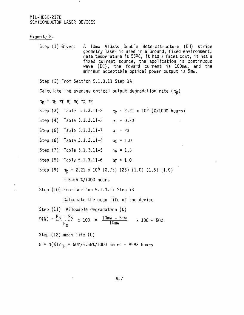
MIL-HDBK-217D SEMICONDUCTOR LASER DEVICES
Example 8.
Step (1) Given: A lOmw AlGaAs Double Heterostructure (DH) stripe geometry laser is used in a Ground, fixed environment, case temperature is 55°C, it has a facet coat, it has a fixed current source, the application is continuous wave (DC), the foward current is lOOma, and the minimum acceptable optical power output is 5mw.
Step (2) From Section 5.1.3.11 Step 1A
Calculate the average optical output degradation rate (Tn)
T p = T b TIJ TTI TTC TTA TTF
Step (3) Table 5.1.3.11-2 rp = 2.21 x 10⁵ (%/1000 hours)
Step (4) Table 5.1.3.11-3 TIT = 0.73
Step (5) Table 5.1.3.11-7 jq = 23
Step (6) Table 5.1.3.11-4 TTC = 1.0
Step (7) Table 5.1.3.11-5 TTA = 1.5
Step (8) Table 5.1.3.11-6 up = 1.0
Step (9) T P = 2.21 x 10⁵ (0.73) (23) (1.0) (1.5) (1.0)
= 5.56 %/1000 hours
Step (10) From Section 5.1.3.11 Step IB
Calculate the mean life of the device
Step (11) Allowable degradation (D)
D(%) = f i _ i i s x 1 0 0 = lOmw^Smw x m = 5Q%
"s
Step (12) mean life (U)
U = D(%)/ip = 50%/5.56%/1000 hours = 8993 hours
A-7

MIL-HDBK-217D SEMICONDUCTOR LASER DEVICES
Step (13) From Section 5.1.3.11 Step 1C
Calculate the average failure rate (X^)
xb = 1/U = 111 F/106 hours
Step (14) From Section 5.1.3.11 Step 2
Calculate the average semiconductor laser failure rate (k)
Xp = b^E = H I F/106 hours (2.4) = 266.4 F/106 hours
A-8

MIL-HDBK-217D TUBES
5.1.4 Tubes, Electronic Vacuum
5.1.4.1 All Types Except Traveling VJave Tubes and Magnetrons. The operating failure rate model (Xp) is:
X p = Xj-, X TTE X TT|_
where
Xp = tube operating failure rate in failures/106 hr. X^ = base failure rate in failures/106 hr and is a function of tube
type and operating parameters (see Table 5.1.4.1-1). TT£ = environmental factor (see Table 5.1.4.1-4). TT[_ = learning factor (see Table 5.1.4.1-5).
TABLE 5.1.4.1-1: b, BASE FAILURE RATE FOR TUBES (includes both random and wearout failures)
TUBE TYPE
RECEIVER Triode, Tetrode, Pentode Power Rectifier
CRT
THYRATRON
CROSSED FIELD AMPLIFIER QK681 SFD261
PULSED GRIDDED 2041 6952 7835
TRANSMITTING Triode ~] peak Pwr<200 kW, Freq<200 MHz, Tetrode & Pentode] [J\ver Pwr£2kW If any of above limits are exceeded
VIDICONS Antimony trisulfide (Sb2S3) photoconductive material Silicon diode array photoconductive material
5.1.4.1-1
Xb (f./106 hrs.)
5 10
9.6
50
260 150
140 390 140
75 100 250
51 48
A-9
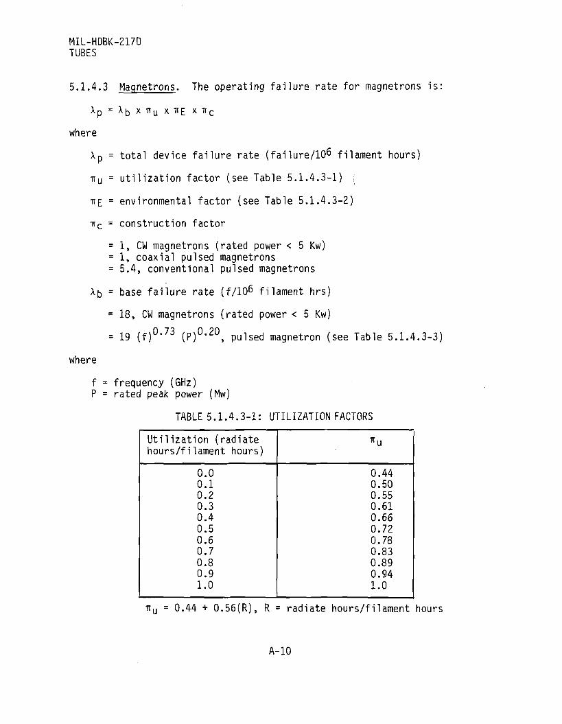
MIL-HDBK-217D TUBES
5.1.4.3 Magnetrons. The operating failure rate for magnetrons is:
Xp = X b x TTU x TTE x TTC
where
Xp = total device failure rate (failure/106 filament hours)
TTU = utilization factor (see Table 5.1.4.3-1)
TTE = environmental factor (see Table 5.1.4.3-2)
TTC = construction factor
= 1, CW magnetrons (rated power < 5 Kw) = 1, coaxial pulsed magnetrons
= 5.4, conventional pulsed magnetrons
X5 = base failure rate (f/106 filament hrs)
= 18, CW magnetrons (rated power < 5 Kw)
= 19 (f) 0- 7 3 (P) 0- 2 0, pulsed magnetron (see Table 5.1.4.3-3)
where
f = frequency (GHz) P = rated peak power (Mw)
TABLE 5.1.4.3-1: UTILIZATION FACTORS
Utilization (radiate hours/filament hours)
0.0 0.1 0.2 0.3 0.4 0.5 0.6 0.7 0.8 0.9 1.0
*u
0.44 0.50 0.55 0.61 0.66 0.72 0.78 0.83 0.89 0.94 1.0
TTU = 0.44 + 0.56(R), R = radiate hours/filament hours
A-10
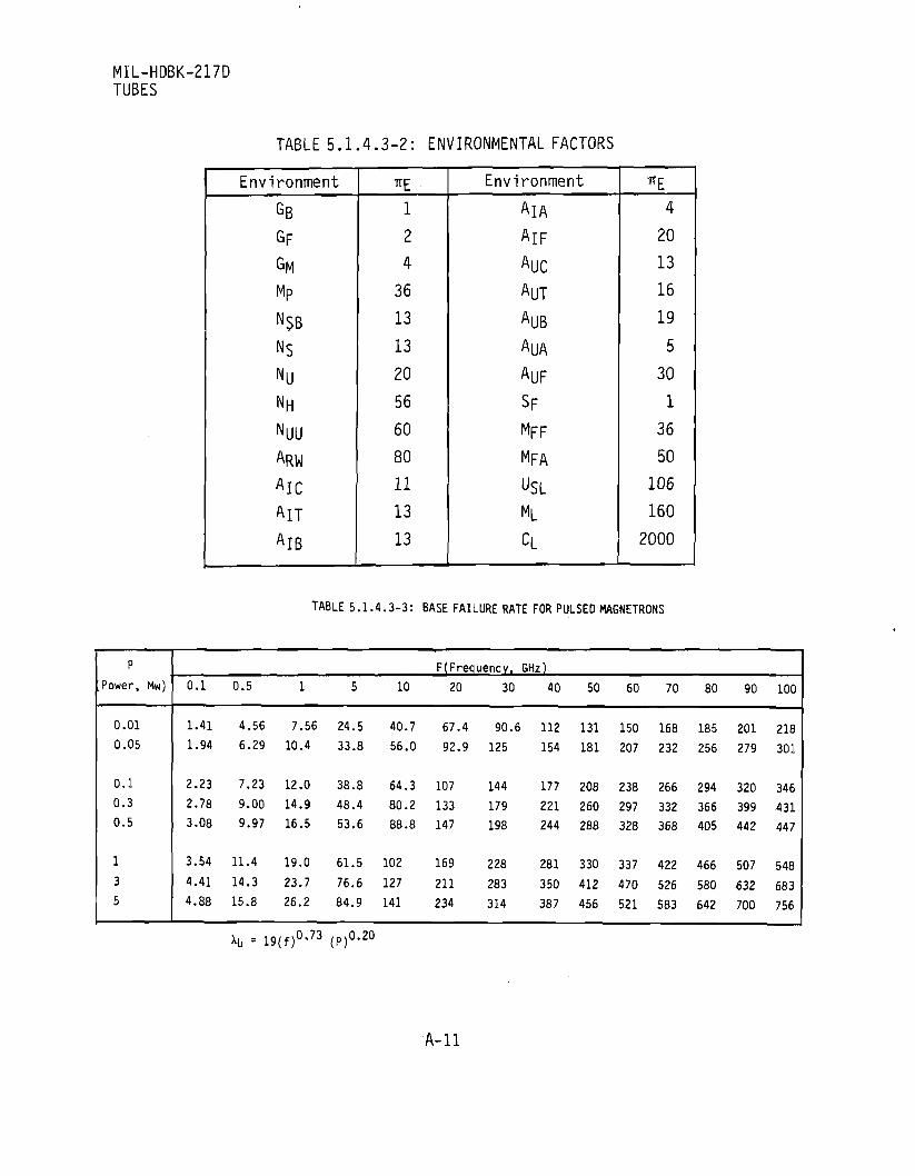
MIL-HDBK-217D TUBES
TABLE 5.1.4.3-2: ENVIRONMENTAL FACTORS
Environment
GB
GF
GM Mp
N$B NS
Nu NH
NUU
ARW
AlC
AIT
AlB
TTE
1
2
4
36
13
13
20
56
60
80
11
13
13
Environment
AlA
AlF
AUC
AUT
AUB
AUA
AUF
SF
MFF
MFA
USL ML
C L
7TE
4
20
13
16
19
5
30
1
36
50
106
160
2000
TABLE 5.1.4.3-3: BASE FAILURE RATE FOR PULSED MAGNETRONS
p
Power, Mw)
0.01
0.05
0.1 0.3
0.5
1
3
5
0.1
1.41
1.94
2.23
2.78
3.08
3.54
4.41
4.88
0.5
4.56
6.29
7.23
9.00 9.97
11.4
14.3
15.8
1
7.56
10.4
12.0
14.9 16.5
19.0
23.7
26.2
5
24.5
33.8
38.8 48.4
53.6
61.5
76.6 84.9
10
40.7
56.0
64.3
80.2
88.8
102
127
141
F(Frequencv, 20
67.4
92.9
107
133 147
169
211 234
30
90.6
125
144
179
198
228
283 314
GHz)
40
112
154
177
221 244
281
350 387
50
131
181
208
260 288
330
412
456
60
150
207
238
297 328
337
470
521
70
168
232
266
332 368
422
526
583
80
185
256
294
366 405
466
580
642
90
201
279
320 399
442
507
632
700
100
218
301
346
431 447
548
683
756
Xb = 19(f)0' 7 3 (P) 0- 2 0
A-ll

Section Section Section Section Section Section
5.1.5.1 5.1.5.2 5.1.5.3 5.1.5.4 5.1.5.5 5.1.5.6
MIL-HDBK-217D LASERS
5.1.5 Lasers. This section presents failure rate models for laser peculiar items used in the following six major classes of laser equipment (see Bibliography Item 40):
Helium/Neon & Helium/Cadmium Argon Ion CO2 Sealed CO2 Flowing Solid State, Nd:YAG Rod Solid State, Ruby Rod
The models and failure rates presented in this section apply to the laser peculiar items only, i.e., those items wherein the lasing action is generated and controlled. In addition to the laser peculiar items, there are other assemblies used with lasers that contain electronic parts and mechanical devices (pumps, valves, hoses, etc.). The failure rates for these parts should be determined with the same procedures as used for other electronic and mechanical devices in the equipment or system or which the laser is a part. The electronic device failure rates are in other parts of this Handbook and the mechanical device failure rates are in Bibliography Item 47.
The laser failure rate models have been developed at the "functional," rather than "piece part" level because the available data were not sufficient for "piece part" model development. Nevertheless, the laser functional models are included in this Handbook in the interests of completeness. These laser models will be revised to include piece part models and other laser types when the data become available.
Because each laser family can be designed using a variety of approaches, the failure rate models have been structured on three basic laser functions which are common to most laser families, but may differ in the hardware implementation of a given function. These functions are the lasing media, the laser pumping mechanism (or pump), and the coupling method.
The general laser failure rate model is:
XLASER = XMEDIA + XPUMP + xC0UPLING
Examples of media-related hardware and influence factors are the solid state rod, gas, gas pressure, vacuum integrity, gas mix, outgassing, and tube diameter. The electrical discharge, the flashlamp, and energy level are examples of pump-related hardware and influence factors. The coupling function contributors are the "Q" switch, mirrors, windows, crystals, substrates, coatings, and level of dust protection provided.
A-12
MIL-HDBK-217D LASERS
The ^puMP term in the ^LASER equation is zero for helium/neon, helium/cadmium argon ion, CO2 sealed and CO2 flowing lasers because the pumping mechanisms for these lasers contain no laser peculiar items. Pumping is accomplished with electronic parts and circuitry. Failure rates for these parts are not included in this section but they should be included in the reliability analysis of the system or equipment containing the laser. Also, some of the terms in the above general ^LASER equation have modifying factors depending upon the laser type. These factors are shown in the following subsections.
A-13

MIL-HDBK-217D LASERS
5.1.5.1 Helium/Neon and Helium/Cadmium Lasers
xp = *E XMEDIA + ^E ^COUPLING
where
^p = the laser failure rate in failures/10^ operating hours.
TE = the environmental application factor, and its value is determined from Table 5.1.5.7-1.
•MEDIA = the failure rate contribution of the lasing media, and its value is 84 failures/10^ operating hours for helium/ neon lasers, and 228 failures/10^ operating hours for helium/cadmium lasers.
^•COUPLING = ">s the failure rate contribution of the laser coupling hardware, and its value is 0.1 failures/10^ operating hours.
It should be noted that the laser failure rate prediction model can be simplified and rewritten as:
XHe/Ne = 84.1 TTE
^He/Cd = 228.1 TTE
5.1.5-2
A-14
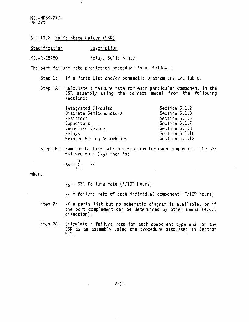
MIL-HDBK-217D RELAYS
5.1.10.2 Solid State Relays (SSR)
Specification Description
MIL-R-28750 Relay, Solid State
The part failure rate prediction procedure is as follows:
Step 1: If a Parts List and/or Schematic Diagram are available.
Step 1A: Calculate a failure rate for each particular component in the SSR assembly using the correct model from the following sections:
Integrated Circuits Section 5.1.2 Discrete Semiconductors Section 5.1.3 Resistors Section 5.1.6 Capacitors Section 5.1.7 Inductive Devices Section 5.1.8 Relays Section 5.1.10 Printed Wiring Assemblies Section 5.1.13
Step IB: Sum the failure rate contribution for each component. The SSR failure rate (xp) then is:
n Xp -.1^ Xi
where
Xp = SSR failure rate (F/106 hours)
Xi = failure rate of each individual component (F/10^ hours)
Step 2: If a parts list but no schematic diagram is available, or if the part complement can be determined by other means (e.g., disection).
Step 2A: Calculate a failure rate for each component type and for the SSR as an assembly using the procedure discussed in Section 5.2.
A-15
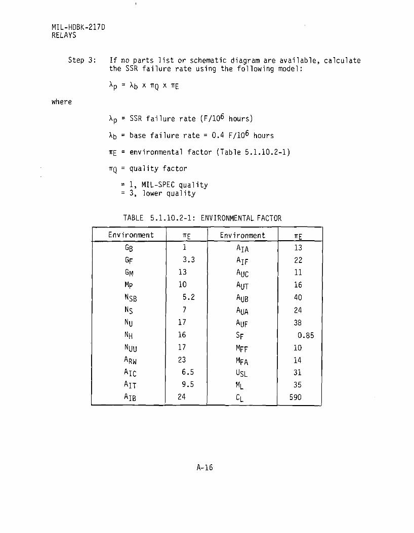
MIL-HDBK-217D RELAYS
Step 3: If no parts list or schematic diagram are available, calculate the SSR failure rate using the following model:
where
Xp = SSR failure rate (F/106 hours)
Xb = base failure rate = 0.4 F/10^ hours
TTE = environmental factor (Table 5.1.10.2-1)
TTQ = quality factor
= 1, MIL-SPEC quality = 3, lower quality
TABLE 5.1.10.2-1: ENVIRONMENTAL FACTOR
Environment
GB
GF
GM Mp
NSB NS Nu NH
NUU ARW
AlC AIT
AlB — — _ _ _ — — — ^ — —
7TE
1
3.3
13
10
5.2
7
17
16 17
23
6.5 9.5 24
Environment
AlA
AlF
AUC AUT
AUB
AUA
AUF
SF MFF
MFA USL ML
cL
TTE
13
22 11
16
40
24
38
0.85
10 14 31
35
590
A-16

MIL-HDBK-217D RELAYS
5.1.10.3 Hybrid and Solid State Time Delay Relays (TDR)
Specification Description
MIL-R-83726 Relay, Time Delay, Hybrid and Solid State
The part failure rate prediction procedure is as follows:
Step 1: If a Parts List and/or Schematic Diagram are available.
Step 1A: Calculate a failure rate for each particular component in the TDR assembly using the correct model from the following sections:
Integrated Circuits Section 5.1.2 Discrete Semiconductors Section 5.1.3 Resistors Section 5.1.6 Capacitors Section 5.1.7 Inductive Devices Section 5.1.8 Relays Section 5.1.10 Printed Wiring Assemblies Section 5.1.13
Step IB: Sum the failure rate contribution for each component. The TDR failure rate (Xp) then is:
n •p ~ .2, Xi
i=l where
Xp = TDR failure rate (F/106 hours)
Xi = failure rate of each individual component (F/IO^ hours)
Step 2: If a parts list but no schematic diagram is available, or if the part complement can be determined by other means (e.g. disection).
Step 2A: Calculate a failure rate for each component type and for the TDR as an assembly using the procedure discussed in Section 5.2.
Step 3: If no parts list or schematic diagram are available and the TDR is a hybrid electronic TDR, calculate the TDR failure rate using the current model for electronic time delay relays (Section 5.1.10).
A-17

MIL-HDBK-217D RELAYS
Step 4: If no parts list or schematic diagram are available and the TDR is an all solid state TDR, calculate the TDR failure rate using the model:
xp = XD + XR
where
xp = TDR failure rate (F/106 hours) l.
^D = delay circuit failure rate (F/10^ hours)
X R = relay circuit failure rate (F/10^ hours)
Step 4A: Calculate the delay circuit failure rate ( XD)
XD = xb x ^E x ^Q
where
^b = base failure rate = 0.5 F/10^ hours
ffE = environmental factor (Table 5.1.10.3-1)
ffn = quality factor = 1 , MIL-SPEC quality = 4, lower quality
Step 4B: Calculate the relay circuit failure rate ( XR) using the procedure given in Section 5.1.10.2.
Step 4C: Calculate the total TDR failure rate ( xp).
*p = XD + *R
A-18

MIL-HDBK-217D RELAYS
TABLE 5.1.10.3-1: ENVIRONMENTAL FACTORS
Environment
GB GF
GM
Mp
NSB Ns
Nu NH NUU ARW
AlC AIT
AlB
TTE
1
4.5
16
12 8.4
8.8 20
18
20
26
8.8 12
35
Environment
AlA
AlF
AUC AUT
AUB AUA
AUF SF
MFF
MFA
USL ML
CL
TTE
18
30
15 21
58
33
52
0.58
12
17
35
40
680
A-19
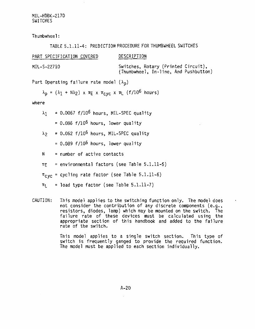
MIL-HDBK-217D SWITCHES
Thumbwheel:
TABLE 5.1.11-4: PREDICTION PROCEDURE FOR THUMBWHEEL SWITCHES
PART SPECIFICATION COVERED DESCRIPTION
MIL-S-22710 Switches, Rotary (Printed Circuit),
(Thumbwheel, In-line, And Pushbutton)
Part Operating failure rate model (Xp)
Xp = ( M + NA2) x TT[: x iTCyC x TT|_ ( f / 1 0 6 hours)
where
Xi = 0.0067 f/106 hours, MIL-SPEC quality
= 0.086 f/106 hours, lower quality
X2 = 0.062 f/106 hours, MIL-SPEC quality
= 0.089 f/106 hours, lower quality
N = number of active contacts
TTE = environmental factors (see Table 5.1.11-5)
7rCyC = cycling rate factor (see Table 5.1.11-6)
TT[_ = load type factor (see Table 5.1.11-7)
CAUTION: This model applies to the switching function only. The model does not consider the contribution of any discrete components (e.g., resistors, diodes, lamp) which may be mounted on the switch. The failure rate of these devices must be calculated using the appropriate section of this handbook and added to the failure rate of the switch.
This model applies to a single switch section. This type of switch is frequently ganged to provide the required function. The model must be applied to each section individually.
A-20
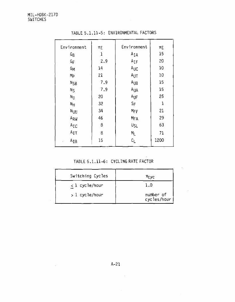
MIL-HDBK-217D SWITCHES
TABLE 5.1.11-5: ENVIRONMENTAL FACTORS
Environment
GB
GF
GM
Mp
NSB NS Ny
NH
NlJU
ARW
AlC AIT
AlB
TTE
1
2.9 14
21
7.9
7.9
20
32
34
46
8
8
15
Environment
AlA
AlF AUC AUT
AUB AUA
AUF
SF MFF MFA
USL
ML
cL
TTE
15
20
10
10
15
15 25
1
21
29
63
71
1200
TABLE 5.1.11-6: CYCLING RATE FACTOR
Switching Cycles
< 1 cycle/hour
> 1 cycle/hour
" cyc
1.0
number of cycles/hour
A-21

TABLE 5.1.11-7: LOAD TYPE FACTOR
Stress
S
0.05
0.1
0.2
0.3
0.4
0.5
0.6
0.7
0.8
0.9
1.0
Resistive
1.00
1.02
1.06
1.15
1.28
1.48
1.76
2.15
2.72
3.55
4.77
Load Type
Inductive
1.02
1.06
1.28
1.76
2.72
4.77
9.49
21.4
Lamp
1.06
1.28
2.72
9.49
54.6
where
r = operating load current rated resistive load
2 n _ (S/.8) for resistive.
2 = e(S/-4) for inductive.
= e(S/.2)2 for lamp.
A-22

MIL-HDBK-217D SWITCHES
Example 3
Given: A MIL-SPEC 2AMP resistive rated thumbwheel switch is installed in an airborne inhabited, cargo environment at a 40°C ambient temperature. The switch has five active contacts. It is cycled an average of 2 cycles per hour, and the load current is 5% of rated current and is resistive. The switch has four %watt, 10 ohm class M carbon composition (RCR) resistors mounted on the switch printed circuit card. The resistors are an integral part of the switch and cannot be removed and replaced if they fail.
Find: The failure rate of the switch as an assembly.
Step 1: Calculate Switch Failure Rate
^1 = 0.0067 f/106 hours
X 2 = 0.062 f/106 hours
N = 5
TTE = 8
71 eye = 2
ffL = 1-02
X p = (Xl + NX 2) X TTE X TT C y C X *L
Xp = (0.0067 + (5 x 0.062)) x 8 x 2 x 1.00
X p = 5.067 f/106 hours
Step 2: Calculate Resistors Failure Rate
From section 5.1.6.1.
Xp = X b x T E x T R x TTQ (f/106 hours)
X b = 0.00055 f/106 hours (40°C, 0.4 stress)
TTE = 3
*R = 1
"Q = 1
A-23

MIL-HDBK-217D SWITCHES
Xp = .00055 x 3 x 1 x 1
= 0.0016 f/106 hours
Step 3: Calculate total switch assembly failure rate
^ = ^switch + 4 x ^resistors
X = 5.067 f/106 hours + 0.006 f/106 hours
X = 5.073 f/106 hours
A-24

MIL-HDBK-217D SWITCHES
5.1.11.2 Circuit Breakers
Specification Description
MIL-C-55629 Circuit Breakers, Magnetic, Unsealed, Trip-Free
MIL-C-83383 Circuit Breakers, Remote Control, Thermal, Trip-Free
MIL-C-39019 Circuit Breakers, Magnetic, Low Power, Sealed, Trip-Free Service
W-C-375 Circuit Breakers, Molded Case; Branch Circuit and
Service
5.1.11.2.1 Prediction Procedure For Circuit Breakers
The part operating failure rate model (Xp) is:
xp = xb x irc x TfQ x TIE
where
Xp = circuit breaker failure rate (F/106 hours)
Xb = base failure rate
= 0.020 failures/106 hours, magnetic circuit breakers = 0.038 failures/106 hours, thermal circuit breakers = 0.038 failures/106 hours, thermal-magnetic circuit breakers
TTC = configuration factor (see Table 5.1.11.2-1)
TTQ = quality factor
= 1.0, MIL-SPEC quality = 8.4, lower quality
TT£ = environmental factor (see Table 5.1.11.2-2)
A-25
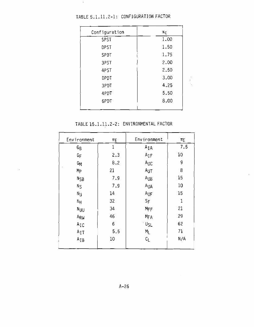
TABLE 5.1.11.2-1: CONFIGURATION FACTOR
Configuration
SPST
DP ST
SPDT
3PST
4PST
DPDT
3PDT
4PDT
6PDT
TTC
1.00
1.50
1.75
2.00
2.50
3.00
4.25
5.50
8.00
TABLE 15.1.11.2-2: ENVIRONMENTAL FACTOR
Environment
GB
GF
GM Mp
NSB NS Ny
NH NUU ARW
AlC AIT
AlB
TTE
1
2.3
8.2
21
7.9
7.9 14
32
34
46 6
5.5 10
Environment
AlA
AlF
AUC AUT
AUB AUA
AUF
SF
MFF
MFA
USL ML
CL
E 7.5
10
9
8 15
10
15
1 21
29
62 71 N/A
A-26

MIL-HDBK-217D INTEGRATED CIRCUIT (IC) SOCKETS
5.1.12.3 Integrated Circuit (IC) Socket Prediction Procedure.
SPECIFICATION DESCRIPTION
MIL-S-83734 Sockets, Plug-in Electronic Components
The part failure rate model is:
X p = Xb x N x TIE
where
X p = total failure rate (f/106 hours)
Xb = base failure rate = 0.000091 f/106 hours N = number of active contacts (active indicates electrical current
flow through the contact) TTE = environmental factor (Table 5.1.12.3-1) and where except for the
environments noted in Table 5.1.12.3-1 socketed device must be restrained
TABLE 5.1.12.3-1: ENVIRONMENTAL FACTORS
Environment
GB
GF
GM
Mp
NSB NS Nil NH NlIU
ARW
AlC
AIT
AlB
TTE
1.0
3.1 17*
11*
5.4
7.3*
18*
17*
19*
25* 6.7*
6.7*
10*
Environment
AlA
AlF AUC AUT
AUB
AUA
AUF SF MFF
MFA
USL
ML
CL
TTE
10*
13*
10*
10*
13*
13*
20* 1.0
11*
16* 33*
39*
650*
* should only be used in this environment if socketed device is restrained.
A-27

MIL-HDBK-217D METERS, PANEL
5.1.15 Meters
5.1.15.1 Prediction Procedure For Meters, Electrical Indicating
Specification Description
MIL-M-10304 Meter, Electrical Indicating, Panel Type, Ruggedized.
The part operating failure rate model (Xp) is:
Xp = Xb(TTA X TTF X TTQ X TT£)
where
Xp = meter failure rate in failures/10^ hours
X5 = base failure rate = 0.090 F/106 hours
TTA = application factor = 1.0, DC Current = 1.7, AC Current
Tip = function factor = 1.0, Ammeter = 2.2, Voltmeter = 2.8, Other (meters whose basic meter movement construction is an
ammeter with associated internal conversion elements)
TTQ = quality factor = 1.0, MIL-SPEC quality = 3.4, lower quality
ff£ = environmental factor (see Table 5.1.15.1-1)
A-28
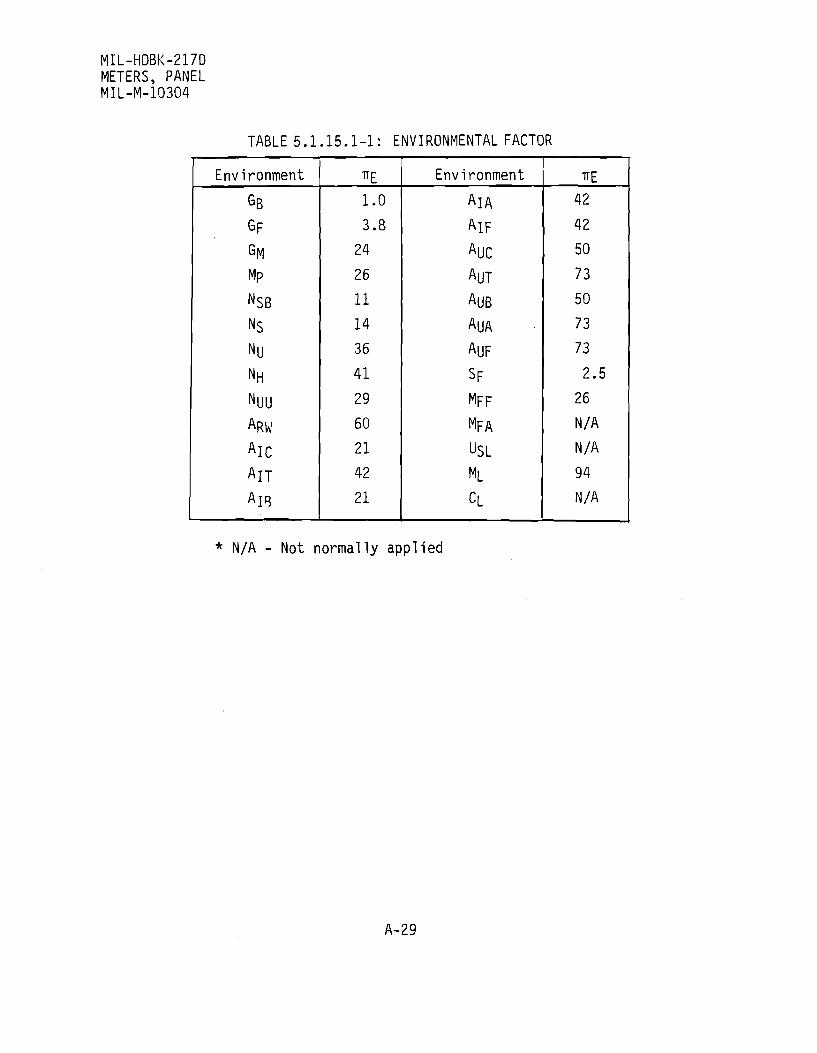
MIL-HDBK-217D METERS, PANEL MIL-M-10304
TABLE 5.1.15.1-1: ENVIRONMENTAL FACTOR
Environment
GB GF GM
Mp NSB NS
Nu NH
NUU ARW
AlC AIT
AlB
TTE
1.0 3.8
24
26
11 14
36
41
29
60
21
42
21
Environment
AlA
AlF
AUC AUT
AUB AUA
AUF
SF
MFF
MFA
USL ML
CL
TTE
42
42
50
73
50
73
73
2.5
26
N/A
N/A
94
N/A
* N/A - Not normally applied
A-29

MIL-HDBK-217D METERS, PANEL
5.1.15.2 Example Failure Rate Calculations
Example 1.
Given: A MIL-M-10304 panel AC ammeter used in an airborne cargo inhabited environment.
Step 1.
The failure rate of the meter is found by substituting the values of Xb, TTA, TTF, TTQ and TTE into the part failure rate model:
Xp = XbUA x TTF x TTQ x TT E) failures/106 hours
X p = 0.90(1.7 x 1.0 x 1.0 x 21) failures/106 hours
X p = 3.213 F/106 hours
Example 2.
Given: A commercial panel type frequency meter with a construction similar to MIL-M-10304 panel meters. The meter operates the same as a DC ammeter. It is used in a ground, mobile application.
Step 1.
The failure rate of the meter is found by substituting the values of Xb» TTA». TTF» U Q and TTE into the part failure rate model:
Xp = XD(TTA X TTF X TTQ x TTE) failures/106 hours
X p = 0.90(1.0 x 2.8 x 3.4 x 24) failures/106 hours
X p = 20.563 F/106 hours
A-30
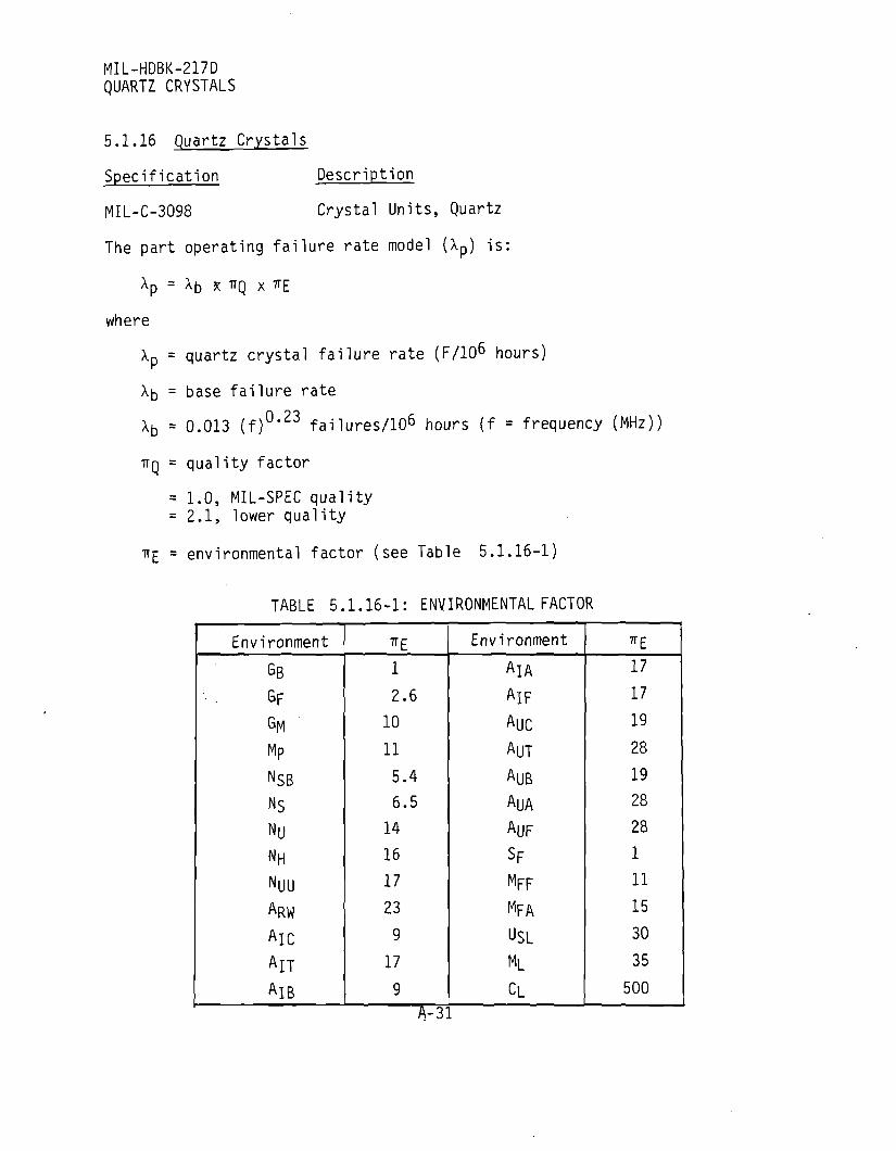
MIL-HDBK-217D QUARTZ CRYSTALS
5.1.16 Quartz Crystals
Specification Description
MIL-C-3098 Crystal Units, Quartz
The part operating failure rate model (Xp) is:
^p = ^b x TTQ x E
where
Ap = quartz crystal failure rate (F/106 hours)
Xb = base failure rate
Ab = 0.013 ( f ) 0 , 2 3 failures/106 hours (f = frequency (MHz))
TTQ = quality factor
= 1.0, MIL-SPEC quality = 2.1, lower quality
fiE = environmental factor (see Table 5.1.16-1)
TABLE 5.1.16-1: ENVIRONMENTAL FACTOR
Environment
GB GF
GM
Mp
NSB
NS Nu NH NUU
ARW
AlC
AIT
AlB
E 1
2.6 10
11 5.4 6.5 14 16 17
23
9
17
9 A-3]
Environment
AlA
AlF AUC
AUT
AUB AUA AUF
SF
MFF
MFA
USL ML
CL
TTE
17
17
19
28
19
28 28 1 11
15
30
35
500

MIL-HDBK-217D LAMPS
5.1.17.1 Lamps, Incandescent
SPECIFICATION
MIL-L-6363
W-L-lll
DESCRIPTION
Lamps, Incandescent, Aviation Service
Lamp, Incandescent, (Electric, Miniature, Tungsten-Filament)
5.1.17.1.1 Prediction Procedure For Incandescent Lamps
The part operating failure rate model (Xp) is:
Xp = Xb X 1TU X TT/\ X 1T£
where
Xp = incandescent lamp failure rate (F/10^ hours)
Xb = base failure rate
Xb = 0.074(Vr)1,29 f/106 hrs. (Vr = rated voltage (volts))
TTU = utilization factor (see Table 5.1.17.1.1-1)
TTA = application factor
= 1.0, AC applications = 3.3, DC applications
TIE = environmental factor (see Table 5.1.17.1.1-2)
TABLE 5.1.17.1.1-1: UTILIZATION FACTORS
Utilization (Illuminate hours/
equipment operate hours)
< 0.10 0.10 to 0.90
> 0.90
u
0.10 0.72 1.0
A-32

MIL-HDBK-217D LAMPS
TABLE 5.1.17.1.1-2: ENVIRONMENTAL FACTORS
Environment
GB
GF
GM
Mp
NSB NS Nu NH
NUU ARW
AlC
AIT
AlB
TTE
1
1.6
3.4
3.5
2.4
2.7 4.1
4.4
4.5 5.3
3.2
4.4
3.2
Environment
AlA
AlF
AUC AUT
AUB
AUA
AUF
SF MFF
MFA
USL ML
CL
TIE
4.4
4.4
4.8
5.8
4.8
5.8
5.8
1.4
3.5 4.2
6.1
6.5
27
A-33

MIL-HDBK-217D LAMPS
5.1.17.3 Examples For Use of Lamp Models
Example 1:
Given:
Step 1
Step 2
Step 3
Step 4
Step 5
Example 2:
Given:
Step 1:
Step 2
Step 3
Step 4
A 6.3 volt incandescent lamp, used as a tail warning radar indicator in the inhabited portion of a fighter aircraft. The voltage source is AC. The ratio of illuminate hours to equipment operate hours is less than 5%.
Calculate the base failure rate (AD)
Ab = 0.074 (6.3)1 , 2 9 = 0.795 F/106 hours
From Table 5.1.17.1.1-1, TTU = 0.10
From Table 5.1.17.1.1-2 Ajp service, TTE = 4.4
Application factor AC service, ir/\ = 1.0
Calculate the total lamp failure rate (An)
A p = A b X T T | j X T T E X T T A
A p = (0.795 x 0.10 x 4.4 x 1.0) F/106 hours
A D = 0.350 F/106 hours
A 12 volt incandescent lamp, used as a power indicator in a ground, fixed environment. The voltage source is DC. The ratio of illuminate hours to equipment operate hours is 1.0.
Calculate the base failure rate (At>)
Ab = 0.074 (12) 1 , 2 9 = 1.83 F/106 hours
From Table 5.1.17.1.1-1, TTU = 1.0
From Table 5.1.17.1.1-2 Gp service, TTE = 1.6
Application factor DC service, TTA = 3.3
A-34

MIL-HDBK-217D LAMPS
Step 5: Calculate the total lamp failure rate (Xp)
Xp = Xb X 1TU X TTE X TTA
Xp = (1.83 x 1.0 x 1.6 x 3.3) F/106 hours
Xp = 9.66 F/106 hours
A-35

MIL-HDBK-217D ELECTRONIC FILTERS
5.1.18 Electronic Filters (Non-tunable) Prediction Procedure
Specification Description
MIL-F-15733 Filters, Radio Frequency Interference MIL-F-18327 Filters; High Pass, Low Pass, Band Pass, Band
Suppression, and Dual Functioning (Non-tunable)
The part failure rate prediction procedure is as follows:
Step 1: If a Parts List and/or Schematic Diagram are available.
Step 1A: Calculate a failure rate for each particular component in the filter assembly using the correct model from the following sections:
Integrated Circuits Section 5.1.2 Discrete Semiconductors Section 5.1.3 Resistors Section 5.1.6 Capacitors Section 5.1.7 Inductive Devices Section 5.1.8 Printed Wiring Assemblies Section 5.1.13 Crystals Section 5.1.16
Step IB: Sum the failure rate contribution for each component. The filter failure rate (Xp) then is:
n Xp =.Z1 Xi
where
Xp = filter failure rate (F/10^ hours)
Xi = failure rate of each individual component (F/10^ hours)
Step 2: If a parts list but no schematic diagram is available, or if the part complement can be determined by other means (e.g. disection).
Step 2A: Calculate a failure rate for each component type and for the filter as an assembly using the procedure discussed in Section 5.2.
A-36

MIL-HDBK-217D ELECTRONIC FILTERS
Step 3: If no parts list or schematic diagram are available, calculate the filter failure rate using the following model:
where
Xp = Xb x TTQ x TTE
Xp = filter failure rate (F/106 hours)
\ = base failure rate
= 0.0219 F/106 hours for MIL-F-15733, ceramic-ferrite construction (styles FL 10-16, 22, 24, 30-32, 34, 35, 38, 41-43, 45, 47-50, 61-65, 70, 81-93, 95, 96)
= 0.120 F/106 hours for MIL-F-15733, discrete LC components (styles FL 37, 53, 74)
= 0.120 F/106 hours for MIL-F-18327, discrete LC components (composition 1)
= 0.265 F/106 hours for MIL-F-18327, discrete LC and crystal components (composition 2)
^E = environmental factor (Table 5.1.18-1)
TTQ = quality factor
= 1, MIL-SPEC quality = 2.9, lower quality
A-37

MIL-HDBK-217D ELECTRONIC FILTERS
TABLE 5.1.18-1: ENVIRONMENTAL FACTOR
Environment
%
GF
GM Mp NSB
NS Nu NH
Nuu
ARW
AlC
AIT
AlB
E 1
2.1
6
6.4
3.7
4.3
7.9
8.7
9.2
11
5.5
8.8
5.5
Environment
AlA AlF
AUC
AUT
AUB AUA
AUF
SF
MFF
MFA
USL ML
CL
TTE
8.8
8.8
10
13
10
13
13
1.7
6.4
8.2 14
16
120
A-38
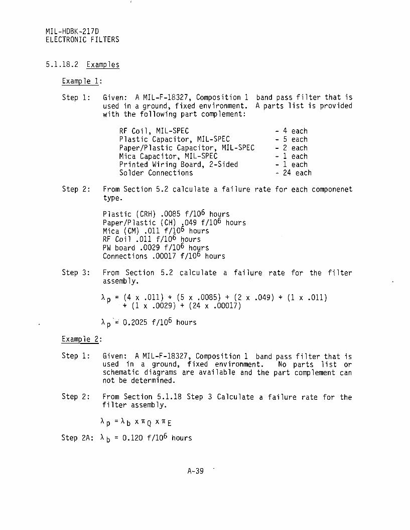
MIL-HDBK-217D ELECTRONIC FILTERS
5.1.18.2 Examples
Example 1:
Step 1: Given: A MIL-F-18327, Composition 1 band pass filter that is used in a ground, fixed environment. A parts list is provided with the following part complement:
RF Coil, MIL-SPEC - 4 each Plastic Capacitor, MIL-SPEC - 5 each Paper/Plastic Capacitor, MIL-SPEC - 2 each Mica Capacitor, MIL-SPEC - 1 each Printed Wiring Board, 2-Sided - 1 each Solder Connections - 24 each
Step 2: From Section 5.2 calculate a failure rate for each componenet type.
Plastic (CRH) .0085 f/106 hours Paper/Plastic (CH) .049 f/106 hours Mica (CM) .011 f/106 hours RF Coil .011 f/106 hours PW board .0029 f/106 hours Connections .00017 f/106 hours
Step 3: From Section 5.2 calculate a failure rate for the filter assembly.
Xp = (4 x .011) + (5 x .0085) + (2 x .049) + (1 x .011) + (1 x .0029) + (24 x .00017)
Xp = 0.2025 f/106 hours
Example 2:
Step 1: Given: A MIL-F-18327, Composition 1 band pass filter that is used in a ground, fixed environment. No parts list or schematic diagrams are available and the part complement can not be determined.
Step 2: From Section 5.1.18 Step 3 Calculate a failure rate for the filter assembly.
X p = X b XTTQ X T T E
Step 2A: X b = 0.120 f/106 hours
A-39

MIL-HDBK-217D ELECTRONIC FILTERS
Step 2B
Step 2C
Step 2D
TTQ = 1
Table 5.1.18-1 TTE = 2 . 1 , GF
Xp = 0.120 f/106 hours x 1 x 2.1
Xp = 0.252 F/106 hours
A-40
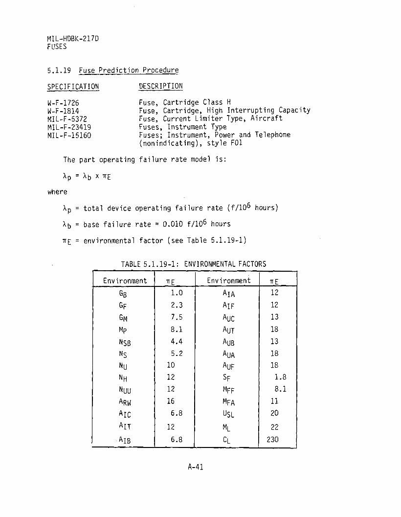
MIL-HDBK-217D FUSES
5.1.19 Fuse Prediction Procedure
SPECIFICATION DESCRIPTION
W-F-1726 W-F-1814 MIL-F-5372 MIL-F-23419 MIL-F-15160
Fuse, Cartridge Class H Fuse, Cartridge, High Interrupting Capaci Fuse, Current Limiter Type, Aircraft Fuses, Instrument Type Fuses; Instrument, Power and Telephone (nonindicating), style F01
The part operating failure rate model is:
X p = X b x TTE
where
X p = total device operating failure rate (f/lO^ hours)
Xb = base failure rate = 0.010 f/106 hours
TTf_ = environmental factor (see Table 5.1.19-1)
TABLE 5.1.19-1: ENVIRONMENTAL FACTORS
Environment
GB GF
GM
Mp
NSB NS Nu NH NUU
ARW
AlC AIT
• A l B
E 1.0
2.3
7.5
8.1
4.4 5.2 10
12 12
16
6.8
12
6.8
Environment
AlA
AlF
AUC AUT
AUB
AUA AUF
sF
MFF
MFA
USL
ML
CL
TTE
12
12
13
18
13
18 18
1.8 8.1
11 20
22
230
A-41