2D MODELLING OF TURBULENT TRANSPORT OF COHESIVE SEDIMENTS IN SHALLOW RESERVOIRS JWL DE VILLIERS A THESIS SUBMITTED IN PARTIAL FULFILMENT OF THE REQUIREMENTS FOR THE DEGREE OF MASTER OF SCIENCE IN ENGINEERING DEPARTMENT OF CIVIL ENGINEERING UNIVERSITY OF STELLENBOSCH DECEMBER 2006

DECLARATION

I declare that this thesis is my own work and that it has not been submitted for a degree at

another university.

JWL de Villiers, 08 / 03 / 2006

ii

ABSTRACT

Modelling of the transport of fine cohesive sediments, as found in most South African

reservoirs, has not been well developed. This is because the transport processes that are

involved are complex and the theories not as implicit as the traditional equilibrium

transport theories for coarse non-cohesive sediment. Advection and dispersion are found to

be the processes that best describe the transport of fine sediments in turbulent flow

conditions.

A two-dimensional modelling tool, MIKE 21C, which simulates reservoir hydrodynamics

and cohesive sediment transport processes with an advection-dispersion model, was

evaluated in this thesis. The creation of such a numerical model involves the setting up of

a suitable curvilinear grid and requires data on the bathymetry, recorded inflows as well as

water levels. It also requires sediment characteristic parameters and transport parameters.

These parameters have to be specified by the user based on previous studies and field

measurement data.

MIKE 21C was applied to laboratory flume tests and reservoir case studies in the field in

order to determine the effects that these parameters have on the sediment transport in a

series of sensitivity studies. Ranges were determined within which these parameter values

should fall. A procedure was also developed through which reservoir sedimentation

models can be calibrated.

iii

OPSOMMING

Die modellering van die vervoer van fyn, kohesiewe sedimente, soos aangetref in Suid

Afrikaanse reservoirs, is nie goed ontwikkel nie. Dit is as gevolg van die komplekse

sedimentvervoerprosesse en teorieë wat nie so implisiet is soos die tradisionele

vervoerteorieë vir growwe, nie-kohesiewe sediment nie. Adveksie en dispersie is die

prosesse wat die vervoer van fyn sediment in turbulente vloei die beste beskryf.

‘n Twee-dimensionele modelleringsagtewarepakket, MIKE 21C, wat reservoirhidro-

dinamika en kohesiewe sedimentvervoerprosesse deur middel van ‘n adveksie-

dispersiemodel simuleer, is in hierdie tesis geëvalueer. Om so ‘n numeriese model op te

stel word ‘n geskikte kurwe-lineêre rooster, opmeetdata van die topografie en gemete data

van die invloeie asook watervlakke benodig. Dit verg ook parameters van die

sedimenteienskappe asook sedimentvervoerparameters. Hierdie parameters moet deur die

gebruiker gespesifiseer word, gebaseer op vorige navorsing en gemete velddata.

Die MIKE 21C sagteware is gebruik om laboratoriumkanaaltoetse en reservoirgevalle-

studies te simuleer en sodoende die invloed wat die parameters op die gesimuleerde

sedimentvervoer het te bepaal in ‘n reeks sensitiwiteitstudies. Sodoende is grense vasgestel

waarbinne die parameterwaardes moet val. ‘n Prosedure is ook ontwikkel waarmee hierdie

reservoirsedimentasiemodelle gekalibreer kan word.

iv

ACKNOWLEDGEMENTS I gratefully acknowledge my study leader, Professor GR Basson of the Department of

Civil Engineering at the University of Stellenbosch, who provided me with assistance and

guidance during the execution of this thesis. I would also like to thank my parents, John

and Elmari, for their tremendous support.

v

TABLE OF CONTENTS

DECLARATION ii ABSTRACT iii OPSOMMING iv

ACKNOWLEDGEMENTS v 1. INTRODUCTION 1 1.1 Background 1 1.2 Domain of this Research 2 1.3 Objectives of this Research 3 1.4 Research Methodology 3 1.5 Limitations of this Research 5

2. RESERVOIR SEDIMENTATION 7 2.1 Background 7 2.2 Sedimentation Measurement Techniques 8 2.2.1 Stream Sampling 10 2.2.2 Reservoir Surveys 11 2.3 Implications of Reservoir Sedimentation 12 2.4 Measures to Deal with Reservoir Sedimentation 14 3. SEDIMENT TRANSPORT AND MATHEMATICAL MODELLING 16 3.1 Background 16 3.2 Turbulent Sediment Transport 17 3.2.1 Incipient Motion 17 3.2.2 The Applied Unit Stream Power Theory 19 3.2.3 Incipient Motion Criteria with the Stream Power Theory 21 3.2.4 Suspended Load and Bed Load 24 3.3 Traditional Equilibrium Sediment Transport Theories 25 3.4 Non-equilibrium Sediment Transport 31 3.4.1 Cohesive Sediment 31 3.4.2 Non-equilibrium Sediment Transport Background 32 3.4.3 Non-equilibrium Sediment Transport Theories for Steady Flow 33 3.5 Advection and Dispersion 38

vi

3.6 Integrated Mathematical Modelling of Unsteady Flow Suspended Sediment Transport and Morphological Change 40 3.6.1 Background 40 3.6.2 Mathematical Model Assumptions 43 3.6.3 One-dimensional Mathematical Modelling 43 3.6.4 The Non-equilibrium Adaptation Length 45 3.6.5 One-dimensional RESSASS Model: Tarbela Reservoir, Pakistan 46 3.6.6 Two-dimensional Mathematical Modelling 48 3.6.7 The Quasi-2D Stream Tube Concept 49 3.6.8 Quasi-2D GSTARS Model: Tarbela Reservoir, Pakistan 52 3.6.9 Three-dimensional Mathematical Modelling 59 3.6.10 Three-dimensional Model: Three Gorges Reservoir Project, China 61 3.7 Density Currents 67 4. THE MIKE 21C MATHEMATICAL SEDIMENTATION MODEL 69 4.1 Background 69 4.2 Basic Setup Parameters 70 4.2.1 Generation of the Curvilinear Grid 70 4.2.2 Bathymetry Development 71 4.2.3 Simulation Period 72 4.2.4 Boundary Specifications 72 4.2.5 Source and Sink 73 4.2.6 Flood and Dry Conditions 73 4.3 Hydrodynamic Parameters 74 4.3.1 Initial Surface Elevation 74 4.3.2 Eddy Viscosity 74 4.3.3 Resistance 75 4.3.4 Helical Flow 75 4.4 Hydrodynamic Integration 77 4.4.1 The Fully Hydrodynamic Module 79 4.4.2 The Quasi-Steady Hydrodynamic Module 81 4.5 Traditional Equilibrium Transport Equations for Non-cohesive Sediments 83 4.5.1 Implementing the Equilibrium Transport Theories 87 4.5.2 The Bed Load Model 88 4.5.3 The Suspended Load Model 88 4.6 The Cohesive Sediment Transport Model 90 4.6.1 The Advection-Dispersion Equation 90 4.6.2 Limitations of the Cohesive Sediment Model 92

vii

4.7 Morphological Change Models 93 4.7.1 Planform Model 93 4.7.2 Alluvial Resistance Model 94 4.7.3 Large-scale Morphological Model 94 4.8 The Selection of Hydrodynamic Module and Models to be Implemented 95 4.8.1 Calibration 95 5. MIKE 21C MODEL VARIABLES 96 5.1 Sensitivity Study Numerical Model Setup 96 5.2 Sediment Particle Size 97 5.3 Sediment Relative Density 97 5.4 Sediment Porosity 98 5.5 Bed Roughness 98 5.6 Settling Velocity 98 5.7 The Stream Wise Advection Constant 100 5.8 Critical Shear Stress for Deposition 101 5.9 Critical Shear Stress for Erosion 103 5.10 Erosion Constant 104 5.11 Exponent of Erosion 106 5.12 Dispersion 107 6. LABORATORY TESTS 108 6.1 Objectives 108 6.2 Design and Methodology 108 6.3 Test Setup 110 6.4 Test Procedure 112 6.5 Calibration 113 6.6 Determining the Sediment Particle Size 115 6.7 Sampling Procedure 116 6.8 Determining the Roughness of the Channel 117 6.9 The Vertical Velocity Profiles for the Test Conditions 118 6.10 Results from the Laboratory Tests 121 7. MIKE 21C SIMULATIONS OF LABORATORY TESTS 122 7.1 Numerical Model Setup 122 7.2 Laboratory Test Model Calibrations 123 7.3 Findings 128

viii

8. LONG TERM NUMERICAL STUDIES OF SEDIMENTATION 130 8.1 Background 130 8.2 Welbedacht Reservoir Model 130 8.2.1 Calibration: 1973 – 1976 132 8.2.2 Validation: 2000 – 2002 141 8.2.3 Long Term Sedimentation Simulations 145 8.3 Vaal Reservoir Model 147 8.3.1 Calibration: 1988 – 2003 148 8.3.2 Validation 161 8.4 Winam Gulf Model, Lake Victoria, Kenya 163 8.4.1 Calibration: 1950 – 2004 165 8.4.2 Validation: the Sediment Core Dating Study 167 9. CONCLUSIONS AND RECOMMENDATIONS 173 9.1 Modelling with MIKE 21C 173 9.1.1 Small Scale Flume Modelling 173 9.1.2 Large Scale Reservoir Modelling 174 9.2 Recommended Parameter Calibration Procedure 177 9.2.1 Sediment Size 177 9.2.2 Settling Velocity 177 9.2.3 Critical Shear Stress for Deposition 177 9.2.4 Critical Shear Stress for Erosion 178 9.2.5 Stream Wise Advection Constant 179 9.2.6 Calibration Data 179 9.3 Research Recommendations 180 10. REFERENCES 181 APPENDICES 189 Appendix A: Laboratory Test Calculations 190 Appendix B: ASTM Method for Determining Particle Size Distribution 194 Appendix C: Laboratory Results 197 Appendix D: Determining the Roughness of the Laboratory Channel 200 Appendix E: Laboratory Test Velocity Distribution Calculations 202 Appendix F: Welbedacht Reservoir Sediment Data 206 Appendix G: Welbedacht Sediment Load Calculations 208 Appendix H: Vaal Reservoir Sediment Data 210

ix

Appendix I: Vaal Reservoir Suspended Sediment Data 215 Appendix J: Nyando River Suspended Sediment Data 218 Appendix K: Nyando Inflow Time-series and Sediment Concentrations 219 LIST OF TABLES xi LIST OF FIGURES xii LIST OF SYMBOLS xv

x

LIST OF TABLES

Table 3-1: Comparison between the calculated and measured deposits for different reaches 64 Table 5-1: Sensitivity study model parameters 96 Table 6-1: The laboratory test flow parameters 109 Table 6-2: Test flow and sediment parameters 112 Table 6-3: Time measurements of the drawdown intervals 114 Table 7-1: The simulation model constants 122 Table 7-2: The simulation model variables and input concentrations 122 Table 7-3: Attempted calibration parameters for Test 1 123 Table 7-4: Attempted calibration parameters for Test 2 124 Table 7-5: Attempted calibration parameters for Test 3 126 Table 7-6: Attempted calibration parameters for Test 4 127 Table 8.2-1: Calibration model variables 135 Table 8.2-2: Validation model variables 142 Table 8.3-1: Model calibration variables 153 Table 8.4-1: Calibration model variables 166 Table 8.4-2: Measured Cs-137 in the cores analysed 170 Table 9-1: The laboratory test and simulation parameters 173 Table 9-2: The reservoir model parameters 176

xi

LIST OF FIGURES

Figure 2-1: Historical growth in storage capacity and sediment deposition worldwide 7 Figure 2-2: Sedimentation of reservoirs in South Africa 9 Figure 3-1: Shields’ diagram 18 Figure 3-2: Variation in power input and applied power 19 Figure 3-3: Critical conditions for cohesionless particles 23 Figure 3-4: Simulated and surveyed longitudinal profile of 48 Tarbela Reservoir Figure 3-5: Tarbela Dam and Reservoir 55 Figure 3-6: Hydrology and dam operation for Tarbela Reservoir 55 Figure 3-7: Two reservoir cross-sections showing uniform sedimentation 56 Figure 3-8: Results of the simulation of the Tarbela delta advancement over a period of 22 years 57 Figure 3-9: Comparison of measurements and GSTARS3 computation for two cross sections in the upstream region of Tarbela Reservoir 58 Figure 3-10: Comparison of measurements and GSTARS3 computation for two cross-sections in the reservoir region of the study reach 58 Figure 3-11: Relative error of the thalweg elevation predictions 59 Figure 3-12: River Configuration in the Dam Area of Three Gorges Project 63 Figure 3-13: Development of the deposition of the entire and near dam reaches 66 Figure 3-14: The plunge line with floating debris where the Nzoia River flows into Lake Victoria, Kenya. 68 Figure 4-1: A curvilinear grid created for a river and reservoir system 71 Figure 4-2: The grid with complete interpolated bathymetry 72 Figure 4-3: Typical time-series of measured reservoir water levels and inflow 73 Figure 4-4: Helical flow in river bends 75 Figure 4-5: The vertical distributions of primary flow and helical flow 76 Figure 4-6: The curvilinear flow parameters 79 Figure 5-1: Sediment concentrations for different settling velocities 99 Figure 5-2: Deposited layer thickness for different settling velocities 99 Figure 5-3: Sediment concentrations for different stream wise constants 100 Figure 5-4: Deposited layer thickness for different stream wise constants 100 Figure 5-5: Sediment concentrations for different shear stresses for deposition 101 Figure 5-6: Deposited layer thickness for different shear stresses for deposition 102 Figure 5-7: Sediment concentrations for different shear stresses for erosion 103 Figure 5-8: Deposited layer thickness for different shear stresses for erosion 103 Figure 5-9: Sediment concentrations for different erosion constants 105 Figure 5-10: Deposited layer thickness for different erosion constants 105 Figure 5-11: Sediment concentrations for different erosion exponents 106 Figure 5-12: Deposited layer thickness for different erosion exponents 106

xii

Figure 6-1: The dry laboratory channel 108 Figure 6-2: A schematic drawing of the laboratory setup 110 Figure 6-3: The sediment dispersing pipe 111 Figure 6-4: The laboratory test setup 111 Figure 6-5: The magnetic flow meter voltage versus pipe discharge 113 Figure 6-6: The particle size distribution of laboratory sediment 115 Figure 6-7: The suspended sediment samplers at their three different measuring depths 116 Figure 6-8: Sampling in progress 117 Figure 6-9: The velocity profile for tests 1 and 2, with an average velocity of 0.1 m/s 120 Figure 6-10: The velocity profile for tests 3 and 4, with an average velocity of 0.05 m/s 120 Figure 6-11: The results from the laboratory tests 121 Figure 7-1: Concentration results of the calibration runs for Test 1 124 Figure 7-2: Concentration results of the calibration runs for Test 2 125 Figure 7-3: Concentration results of the calibration runs for Test 3 126 Figure 7-4: Concentration results of the calibration runs for Test 4 127 Figure 7-5: The vertical velocity profiles of turbulent flow and a density current 128 Figure 8.2-1: The observed loss in storage capacity of Welbedacht Reservoir 131 Figure 8.2-2: The longitudinal profiles of Welbedacht Reservoir 131 Figure 8.2-3: An aerial photo of Welbedacht Reservoir 132 Figure 8.2-4: The curvilinear grid (in plan) used in the Welbedacht model 132 Figure 8.2-5: The 1973 bathymetry (in plan) used in the Welbedacht model 133 Figure 8.2-6: Median particle sizes of bed grab samples taken along Welbedacht reservoir 134 Figure 8.2-7: The 1973 to 1976 time-series for the model’s inflow and downstream water level based on observed data 135 Figure 8.2-8: Deposited sediment layers at section 41 for different settling velocities 136 Figure 8.2-9: Deposited sediment layers at section 26 for different settling velocities 137 Figure 8.2-10: Deposited sediment layers at section 9 for different settling velocities 137 Figure 8.2-11: Deposited sediment layers at section 41 for different shear stresses for deposition 138 Figure 8.2-12: Deposited sediment layers at section 26 for different shear stresses for deposition 139 Figure 8.2-13: Deposited sediment layers at section 9 for different shear stresses for deposition 139 Figure 8.2-14: Deposited sediment layers at section 41 for different stream wise constants 140 Figure 8.2-15: Deposited sediment layers at section 26 for different stream wise constants 140 Figure 8.2-16: Deposited sediment layers at section 9 for different stream wise constants 141 Figure 8.2-17: The 2000 survey bathymetry used for the validation 142 Figure 8.2-18: The 2000 to 2002 time-series for the model’s inflow and downstream water level 143 Figure 8.2-19: Deposited sediment layers at section 41 for the validation simulation 143

xiii

Figure 8.2-20: Deposited sediment layers at section 26 for the validation simulation 144 Figure 8.2-21: Deposited sediment layers at section 9 for the validation simulation 144 Figure 8.2-22: Historic longitudinal bed profiles with future sedimentation levels 145 Figure 8.2-23: The simulated 2029 bathymetry in plan 146 Figure 8.2-24: Section 41 profile and flood levels 147 Figure 8.3-1: An aerial photo of Vaal Reservoir 148 Figure 8.3-2: The curvilinear grid used for the Vaal Reservoir model 149 Figure 8.3-3: The original 1988 surveyed bathymetry 149 Figure 8.3-4: The grab sediment sampler with a typical load of cohesive sediment from Vaal Reservoir 150 Figure 8.3-5: The bed sediment particle size distribution 150 Figure 8.3-6: 1993-1995 Measured suspended sediment yield/discharge data and the trendline 151 Figure 8.3-7: The 1988 to 2003 time-series for the model’s inflow and water level based on observed data 153 Figure 8.3-8: The upstream input sediment concentration time series 154 Figure 8.3-9: Deposited sediment layers at section 51 for different settling velocities 155 Figure 8.3-10: Deposited sediment layers at section 30 for different settling velocities 155 Figure 8.3-11: Deposited sediment layers at section 2 for different settling velocities 155 Figure 8.3-12: Deposited sediment layers at section 51 for different shear stresses for deposition 156 Figure 8.3-13: Deposited sediment layers at section 30 for different shear stresses for deposition 157 Figure 8.3-14: Deposited sediment layers at section 2 for different shear stresses for deposition 157 Figure 8.3-15: Deposited sediment layers at section 51 for different stream wise constants 158 Figure 8.3-16: Deposited sediment layers at section 30 for different stream wise constants 159 Figure 8.3-17: Deposited sediment layers at section 2 for different stream wise constants 159 Figure 8.3-18: Deposited sediment layers at section 51 for the parameter variations 160 Figure 8.3-19: Deposited sediment layers at section 30 for the parameter variations 160 Figure 8.3-20: Deposited sediment layers at section 2 for the parameter variations 160 Figure 8.3-21: Simulated and measured concentrations versus discharge upstream of Vaal Marina 161 Figure 8.3-22: Vaal Reservoir Inflow Time-series 161 Figure 8.4-1: A satellite image of the Winam Gulf study area 163 Figure 8.4-2: The curvilinear grid of the Winam Gulf study area 164 Figure 8.4-3: The 2005 surveyed bathymetry superimposed on the grid 164 Figure 8.4-4: Nyando river measured concentrations versus discharge 165 Figure 8.4-5: The 1950 to 2004 time-series for the Nyando River inflow and the Rusinga Channel water level based on observed data 166 Figure 8.4-6: The original locations of the core samples 168 Figure 8.4-7: Historical Cs-137 fallout 169 Figure 8.4-8: The simulated 54 year accumulated sediment layer thickness 172 Figure 8.4-9: A satellite image showing the movement of sediment laden water through the gulf 172

xiv

LIST OF SYMBOLS A flow cross-section A Ackers and White equation coefficient α coefficient by Yang (1984) α adjustment coefficient (Falconer and Owens, 1990) α non-equilibrium adaptation or recovery coefficient α helical flow calibration constant a calibration parameter that can be interpreted as mean settling depth a reference level at which the bed concentration is determined

1α coefficient by Rooseboom (1975) 2α coefficient by Rooseboom (1975)

01α stream wise advection constant

02α secondary flow advection constant

1a - bed load coefficients by Meyer-Peter and Muller (1947) 8a

3α 4α coefficients by Yang (1973)

5α 6α coefficients by Yang (1973)

bxα , byα direction cosines of the bed shear stresses a ,b alluvial resistance model calibration coefficients β parameter by Rozovskii β constant by Yang (1984)

iβ percentage of a sediment fraction in the bed composition by de Silvio (1995) C Chezy friction factor

bC bed load concentration

eqC constant equilibrium concentration *eqC ratio of relative equilibrium concentration

aC reference concentration

dC drag coefficient

oC maximum bed concentration (van Rijn, 1984)

oC initial value of sediment concentration (Mehta and Partheniades, 1973) C total load sediment concentration

*ciC the transporting capacity of a sediment fraction

tkC section averaged sediment concentration

*tkC the suspended load transport capacity

tkC depth-averaged sediment concentration *C equilibrium sediment transport kC depth-averaged suspended load concentration

*kC suspended load transport capacity *kC potential transport capacity of size class k of suspended load

xv

* jCT average concentration of sediment transporting capacity c concentration ca bed layer concentration (Falconer and Owens, 1990)

'c Ackers and White equation coefficient bc the reference concentration near the bed

ec equilibrium concentration

kc local concentration of the k-th size class of suspended sediment load

*b kc equilibrium concentration at the reference level z.

bkc average concentration of bed load at the bed load zone D depth of flow DL grain size of a sediment group

*D dimensionless particle diameter

TxxD turbulence coefficients in x direction

TyyD turbulence coefficients in y direction

TxyD turbulence coefficients in the transverse direction xxD dispersion in the x-direction (includes advection and turbulent diffusion) yyD dispersion in the y-direction (includes advection and turbulent diffusion)

Dxx, Dxy, dispersion terms due to the effect of secondary flow Dyx, Dyy dispersion terms due to the effect of secondary flow

bkD deposition rate

50d median particle diameter

grd Ackers and White dimensionless sediment particle size dj Soares sediment particle diameter d particle diameter Δ step height for the vertical velocity profile

bδ saltation height δs deviation in stream direction due to helical flow δ bed load layer thickness

3jδ Kronecker delta E eddy viscosity

bkE entrainment rate E erosion rate

0E erosion constant ∈ coefficient of turbulent exchange

1ξ sediment transport under non-equilibrium conditions for deposition

2ξ sediment transport under non-equilibrium conditions for erosion

sε Turbulence diffusivity coefficient of sediment F van Rijn coefficient Fr Froude number Fi external forces including gravity per unit volume Fs entrainment function

grF Ackers and White a mobility number

cf Coriolis coefficient

xvi

grG Ackers and White sediment transport function g gravitational acceleration

sγ specific weight of sediment γ specific weight of water H water level h water depth I bed slope or slope of water surface si helical flow intensity

3K empirical coefficient by Zhang (1959)

4 K empirical coefficient by Zhang (1959)

5K empirical coefficient by Zhang (1959) k representative sediment size class κ Von Karman constant

sk absolute bed roughness *i

L adaptation length for a sediment fraction l mixing length

bλ linear sediment concentration M Manning’s roughness M m coefficient of erosion m Ackers and White equation coefficient m parameter related to sediment concentration by Zhang (1959) μ dynamic viscosity of water

dμ dynamic friction coefficient (Engelund and Fredsoe, 1976) N total number of size classes n Ackers and White equation coefficient n sediment porosity n secondary orthogonal coordinate axis n Manning’s roughness n η non-dimensional vertical coordinate of the velocity profile

oη no slip level P wetted perimeter PL percentage by weight of the sediment group p pressure p probability of a moving sediment particle

'p bed material porosity

bkp availability factor of sediment

bkp bed material gradation at the mixing layer ,p q flux field of curvilinear n and s axis 'p , modified curvilinear flux field 'q

ψ suspension parameter correction coefficient φ coefficient used in Engelund Hansen equation (1976) φ depth integrated transport capacity Q discharge

sQ sediment flux

xvii

tkQ actual sediment transport rate

*t kQ sediment transport capacity or the so-called equilibrium transport rate

lkq side inflow or outflow sediment discharge from bank or tributary streams per unit channel length

sq suspended sediment unit flux

bq bed load sediment unit flux q unit flux

sq sediment discharge per unit width at the exit

stq sediment carrying capacity

0sq sediment discharge per unit width at the entrance *bkq potential transport capacity of size class k of bed load j

dq , jeq fluxes of deposition and erosion of sediment

tkxq , components of the total load sediment transport in the x- and y- directions tkyqΦ section averaged transport capacity

blΦ non-dimensional bed load transport rate

slΦ suspended sediment load

sR , nR radius of curvature of s- and n-line, respectively R hydraulic radius Re Reynold’s number

0R radius of eddies formed against bed ρ density of water

sρ particle density

blS bed load transport rate

slS suspended load transport rate tlS total sediment transport load xS , dispersion terms to account for the effect of the non-uniform distributions of yS

flow velocity and sediment concentrations s slope s primary orthogonal coordinate axis ss source/sink term for advection-dispersion equation T width of flow (Soares, 1982) Txx, Txy, depth-averaged turbulent stresses Tyx, Tyy depth-averaged turbulent stresses T transport stage parameter t time τ bed shear stress

cdτ critical shear stress for deposition

ijτ turbulent stresses determined by a turbulence model

ceτ critical shear stress for erosion

cmeτ critical shear stress for mass erosion

minbτ threshold value of bed shear stress

xviii

bxτ , byτ bed shear stresses in the x- and y- directions

sxτ , syτ shear stresses on the water surface caused by wind θ Shield’s parameter θ coefficient used in Engelund Hansen equation (1976)

'θ non dimensional skin shear stress tanα ratio of tangential shear to normal force tan δs limiting angle between average and helical flow shear stress directions

vτ stream power U depth-averaged flow velocity

'fU friction velocity related to skin friction

gu bed shear velocity u mean flow velocity ui- velocity components (i = 1, 2, 3)

*u friction velocity 'fu friction velocity related to skin friction

bsu particle velocity

,f cru Shield’s critical bed shear velocity V volume V section-averaged flow velocity

vV volume of voids in a material Vss settling velocity v velocity v average velocity

crvs the critical input stream power for incipient motion υ kinematic viscosity of water w settling velocity x cartesian coordinate y cartesian coordinate y vertical distance from the bed

0y distance from bed where velocity mathematically equals zero

1y rotational point distance from the bed Z Rouse suspension parameter Z’ modified suspension number z Cartesian coordinate

1z suspension theory coefficient as derived by Rooseboom (1975) 'z suspension theory coefficient

zs water surface elevation

xix

1

1. INTRODUCTION

1.1 Background

Sediment is any particulate matter that can be transported by fluid flow and which is

eventually deposited as a layer of solid particles on the bed of a body of water.

Sedimentation is the deposition by settling of suspended material. Sedimentation

occupies an important position in the field of civil engineering because it determines

the life span and affects the function of many hydraulic projects. Studying reservoir

sedimentation is important to determine capacity loss, the useful life of the reservoir,

and the impact that dam operations have on the reservoir’s deposition pattern.

Sediments in reservoirs are heterogeneous mixtures of soil particles and rock

fragments, detached from the earth’s crust, transported and deposited in the reservoir

basin. Mineral sediments are predominant as either cohesive or non-cohesive solid

materials, coming into the reservoir from the river-catchment system, as a result of the

erosive action of water, air, ice and human activities on the Earth’s surface.

Damming created by the construction of a dam causes reduced sediment transport

capacity in the waters upstream of the dam and the result is therefore sediment

deposition. This causes a gradual loss of live storage capacity as well as a reduced

firm abstraction yield from the reservoir.

The cohesive sediments are relatively homogeneous conglomerates of very fine clay

and silt particles, which are bound by electro-chemical forces (cohesion). The non-

cohesive sediments are non-homogeneous mixtures of sand, gravel, and fractions of

rock. The ratio between cohesive and non-cohesive sediments in a reservoir depends

mainly on the climatic conditions, geological structure, vegetation growth and human

activities in the region.

The percentage fine material found in the bed sediments can have a profound effect

on the sediment transport characteristics of the bed sediments. It has been found that

as little as 7% clay and silt in sediment means that the sediment will effectively have

2

the properties of cohesive sediments (Beck and Basson, 2003). This means that the

sediments are much more resistant to erosion, especially after they have been allowed

to consolidate.

Although many models have been developed for suspended sediment transport,

modelling of the transport of cohesive sediment as found in most South African

reservoirs, is still not well developed.

1.2 Domain of this Research

Turbulent suspended sediment and density current sediment transport have been

identified as the main sediment transport processes for fine sediment through most

South African reservoirs. The occurrence of density currents are very seldom and only

exists under very specific circumstances while turbulence is the mechanism for 96%

of all sediment transport (Rooseboom, 1992).

Numerous theories and equations have been developed for the calculation of

equilibrium sediment transport in turbulent flow. These were developed and calibrated

for the transport of coarse sediments only. Various theories for non-equilibrium

transport have also been established for steady flow conditions. Because of the highly

dynamic nature of sedimentation processes within reservoirs, this research

investigates the calibration of an unsteady two-dimensional (2D) advection-dispersion

equation as implemented by the MIKE 21C software. MIKE 21C is a 2D curvilinear

modelling tool for the simulation of the hydrodynamics and morphological changes in

rivers and reservoirs, developed by the Danish Hydraulic Institute (DHI).

MIKE 21C simultaneously solves the fully dynamic 2D St.Venants equations of

continuity and momentum and the 2D advection-dispersion equation for sediment

transport. The advection-dispersion equation is solved continuously with the dynamic

output of two-dimensional flux, water level and bed level from the hydrodynamic

module. The MIKE 21C modelling tool requires that various transport calibration

parameters are specified. It also requires that detailed sediment characteristics are

specified by the user.

3

This study is therefore directed at the calibration of non-equilibrium dynamic

modelling of turbulent sediment transport of cohesive sediment in reservoirs.

Basson (1996) calibrated the one-dimensional (1D) unsteady advection-dispersion

equation for various sediment types using measured flume data and the 1D MIKE 11

simulation model. This study aims to calibrate a 2D advection-dispersion equation as

implemented in the MIKE 21C software for flume and large scale reservoir

applications. Calibration of a numerical model comprises the adjustment for a

particular situation by making use of some measured data. The parameters of flow,

sediment characteristics and sediment transport will be investigated and calibrated for

varying laboratory and reservoir case studies.

1.3 Objectives of this Research

This research investigates the 2D modelling of cohesive sediment transport using the

MIKE 21C software.

The calibration process for the MIKE 21C hydrodynamic and morphologic model

involves the tuning of a number of calibration factors for each simulation. All the

calibration factors have physical meanings and should not be arbitrarily given values

outside their realistic ranges to obtain agreement with observed data.

These parameters include the sediment characteristics, the flow parameters as well as

the parameters of sediment transport, as required by the advection-dispersion model.

It is the aim of this research to produce insight into the modelling of cohesive

sediment transport in reservoirs so that accurate predictions of sedimentation can be

made which can be used in the design and operation of reservoirs.

1.4 Research Methodology

A study into the traditional equilibrium theories for coarse, non-cohesive sediment

transport was carried out. This is considered as necessary background as it gives

insight into the hydraulic processes that causes sediment deposition and entrainment.

4

The non-equilibrium sediment transport theories for cohesive sediments are then

investigated in detail. Recent developments in this field can be simplified to the

following three modelling methods:

One-dimensional modelling of turbulent transport with advection and

dispersion as implemented in MIKE 11

Two-dimensional modelling of turbulent transport with advection and

dispersion as implemented in MIKE 21C

Three dimensional modelling of turbulent transport with advection and

dispersion.

Examples of numerical models for each of these methods are discussed. MIKE 21C is

then applied on a small scale to model flow in a laboratory flume before it is applied

to model the sedimentation in large bodies of water.

Firstly a straight rectangular glass flume with steady uniform turbulent flow

conditions was modelled. A constant sediment concentration was added at the

upstream boundary. A sensitivity study was then conducted to investigate the working

of the transport parameters and also to establish likely ranges of their values.

Four laboratory tests were then carried out in a rectangular glass flume for varying

conditions of turbulent flow and different initial upstream sediment concentrations.

The concentrations were measured at regular intervals along the flume to monitor the

decreasing suspended sediment concentration. Numerical models were then created in

MIKE 21C to simulate these laboratory conditions. The model’s sediment and

transport parameters were then calibrated so that the numerical models produced

similar results to the laboratory tests.

The field where the MIKE 21C software is most likely to be used is reservoir

sedimentation. Numerical models were created for two South African reservoirs,

Welbedacht Reservoir and Vaal Reservoir. These two are considered very different

regarding size, hydraulics, sediment load and transport characteristics. The purpose

was to calibrate both of these models and thereby determine the suitability of the

software for the modelling of South African reservoirs.

5

Another model was created for Winam Gulf of Lake Victoria in Kenya. The sediment

processes within the gulf are considered to be the same as in a shallow reservoir, and

can therefore be modelled in the same way. All three bodies of water are experiencing

sedimentation of fine cohesive particles.

As part of this research, field work was conducted during 2004 and 2005 at these

three locations to gain information on sediment characteristics. Bed grab samples and

suspended sediment samples were taken throughout these bodies of water to calibrate

their numerical models’ sediment characteristics. Measured flow and water level data

were obtained from different water authorities.

1.5 Limitations of this Research

The version of MIKE 21C that was available for this research was specifically

designed by DHI for the modelling of cohesive sediment in reservoirs using

the advection-dispersion equation. It allows the user to model the transport of

one sediment size fraction only during a simulation. This particle size has to

be representative of the real sediment size distribution. In the latest MIKE 21C

package as well as the one-dimensional MIKE 11, a number of representative

size fractions of clay and silt can be modelled simultaneously.

This MIKE 21C version incorporates a number of shortcuts. Only some of the

sediment transport parameters can be defined by the user. The others, such as

the horizontal dispersion coefficients are calculated by the model itself based

on the flow profiles. This creates a limitation to this methodology in that these

parameters cannot be calibrated. It also greatly simplifies the research.

The computational time for some simulations exceeded a week, while others

needed only a few minutes. The average run time for the reservoir models was

around 15 hours. This limited the number of calibration runs that could be

completed in the allowed research time.

6

The MIKE 21C package does require of the user to build up experience in the

usage of the software before attempting large scale applications such as

reservoirs. Creating a suitable curvilinear grid, for instance, can take a

considerable amount of time and experience.

7

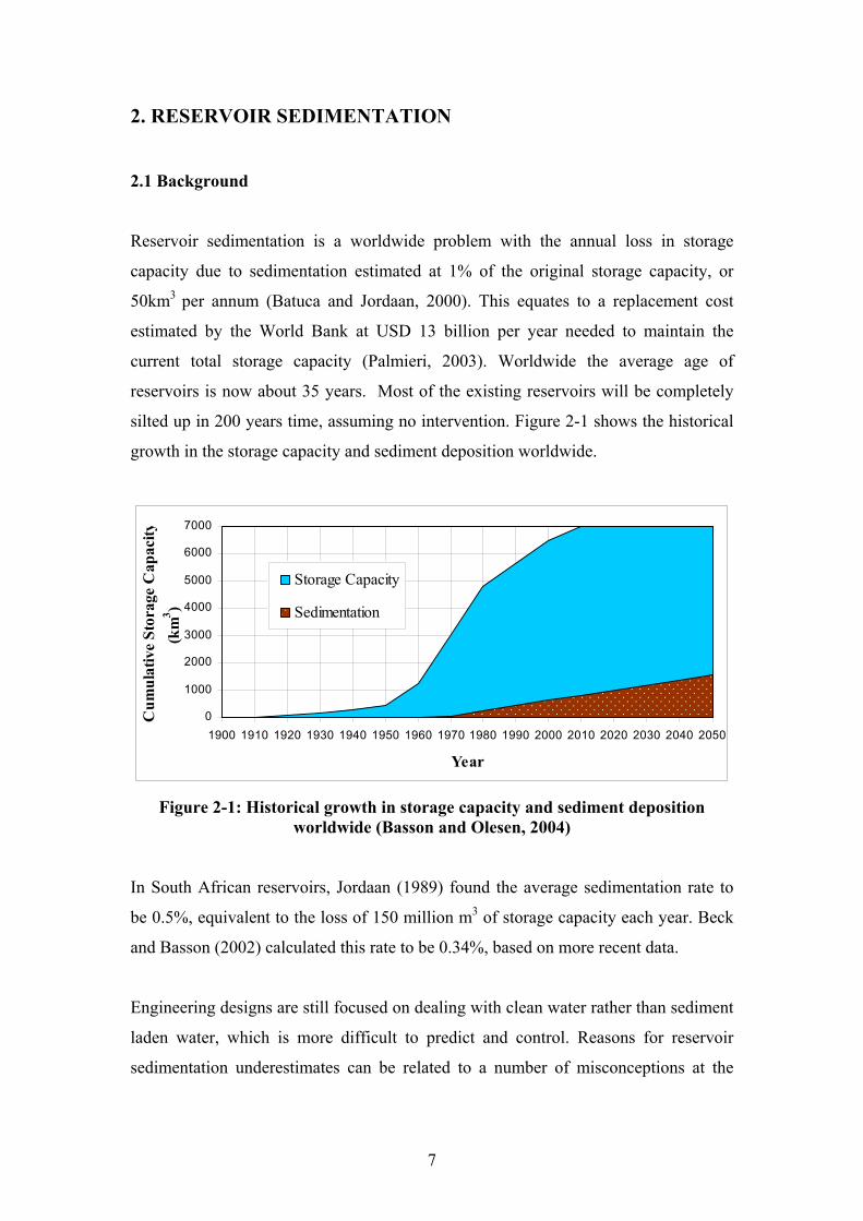
2. RESERVOIR SEDIMENTATION 2.1 Background Reservoir sedimentation is a worldwide problem with the annual loss in storage

capacity due to sedimentation estimated at 1% of the original storage capacity, or

50km3 per annum (Batuca and Jordaan, 2000). This equates to a replacement cost

estimated by the World Bank at USD 13 billion per year needed to maintain the

current total storage capacity (Palmieri, 2003). Worldwide the average age of

reservoirs is now about 35 years. Most of the existing reservoirs will be completely

silted up in 200 years time, assuming no intervention. Figure 2-1 shows the historical

growth in the storage capacity and sediment deposition worldwide.

0

1000

2000

3000

4000

5000

6000

7000

1900 1910 1920 1930 1940 1950 1960 1970 1980 1990 2000 2010 2020 2030 2040 2050

Year

Cum

ulat

ive

Stor

age

Cap

acity

(km

3 )

Storage Capacity

Sedimentation

Figure 2-1: Historical growth in storage capacity and sediment deposition

worldwide (Basson and Olesen, 2004) In South African reservoirs, Jordaan (1989) found the average sedimentation rate to

be 0.5%, equivalent to the loss of 150 million m3 of storage capacity each year. Beck

and Basson (2002) calculated this rate to be 0.34%, based on more recent data.

Engineering designs are still focused on dealing with clean water rather than sediment

laden water, which is more difficult to predict and control. Reasons for reservoir

sedimentation underestimates can be related to a number of misconceptions at the

8

time of reservoir design, and can be grouped into sediment yield misjudgements and

engineering problems (Basson and Rooseboom, 1997):

The sediment yield misjudgements are due to:

Small or short data bases of river sediment transport data or reservoir surveys

Limited information on regional sediment yields linked to soil types,

topography and climatic variables

Land-use changes and increased erosion and sediment yields.

Engineering problems have occurred due to incorrect prediction of reservoir sediment

trap efficiency resulting from:

Overestimation of sediment transporting capacity through reservoirs

Overestimation of the efficiency of outlet structures to sluice/flush sediment

from the reservoirs

Changed operation during the life of reservoirs

Overestimation of the effectiveness of soil conservation schemes in the

catchment.

Worldwide there are many cases where extreme sedimentation has reduced a

reservoir’s lifespan to only a few years. A well known example of where these

problems have occurred in South Africa is Welbedacht Reservoir on the Caledon

River in the Free State Province. This dam was constructed in 1973 with the purpose

of supplying water to the city of Bloemfontein via the 115 km long Caledon-

Bloemfontein pipeline. By 1988, 15 years after construction, it had already lost 73.2

% of the original storage capacity at an average annual sedimentation rate of 4.5 %

(Clarke, 1990).

Flushing operations were carried out but with limited success. The reduction in

storage created problems in meeting the city of Bloemfontein’s demand at an

acceptable level of reliability and as a result, the 50m high off-channel Knellpoort

Dam had to be constructed in 1988. By 2002 Welbedacht Reservoir had lost 89.9% of

it’s original storage capacity (DWAF, 2006). It can be seen in Figure 2-2 that

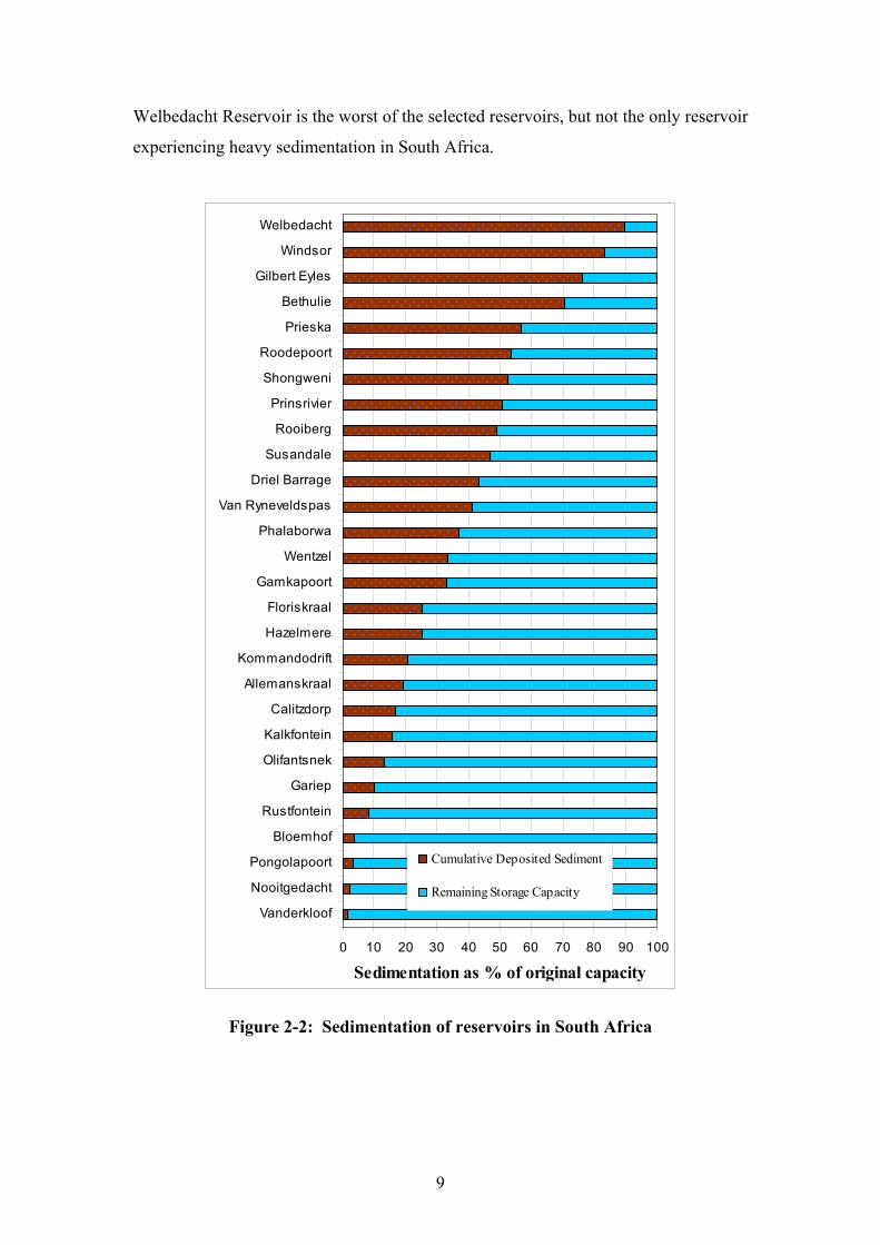
9

Welbedacht Reservoir is the worst of the selected reservoirs, but not the only reservoir

experiencing heavy sedimentation in South Africa.

0 10 20 30 40 50 60 70 80 90 100

Vanderkloof

Nooitgedacht

Pongolapoort

Bloemhof

Rustfontein

Gariep

Olifantsnek

Kalkfontein

Calitzdorp

Allemanskraal

Kommandodrift

Hazelmere

Floriskraal

Gamkapoort

Wentzel

Phalaborwa

Van Ryneveldspas

Driel Barrage

Susandale

Rooiberg

Prinsrivier

Shongweni

Roodepoort

Prieska

Bethulie

Gilbert Eyles

Windsor

Welbedacht

Sedimentation as % of original capacity

Cumulative Deposited Sediment

Remaining Storage Capacity

Figure 2-2: Sedimentation of reservoirs in South Africa

10

2.2 Sedimentation Measurement Techniques

There are basically two techniques to measure sedimentation rates. These are stream

sampling and reservoir surveys.

2.2.1 Stream Sampling

In South Africa, river sediment sampling was initiated in 1919 and daily sampling

programmes were initiated up until the 1970’s. The sampling was mostly done by

filling bottles just below the surface of the stream. The question arises whether these

daily samples can be representative of the daily sediment load of a deep and wide

river.

Studies by Rooseboom (1975) showed that concentrations varied little with depth and

only slightly across a stream. He also found that a correction factor of 1.25 provides

for the tendency of bottled samples to under-represent actual concentrations and it

also brings into account the bed load sediment and changes in concentrations with

depth and width. In the 1950’s depth integrated and bed load sediment samplers were

developed with which the total load can be determined with greater accuracy.

Available data of sediment concentrations upstream of a reservoir can be compared to

the measured discharge into the reservoir at the time that the sample was taken and a

relationship can be established between the two in the form of a simple dependency

equation. Using this equation, sediment concentrations can then be found for any

discharge. The sediment flux, sQ , is found by multiplying the concentrations with the

measured discharges. The total sediment volume that flowed into the reservoir over a

certain period can then be derived by integrating a time-series graph of the sediment

flux.

Even with very low flow velocities within South African reservoirs, concentrations

are rarely lower than 0.001% by mass. During flood conditions this value vary

between 0.1% and 3%, with the high values of 6.5% recorded at Jammersdrift, just

upstream of Welbedacht Reservoir (Rooseboom, 1992), and 9.6% recorded on the

Olifants River (Limpopo Province) in 1996 (Basson, 1996).

11

2.2.2 Reservoir Surveys

Since the 1970’s the emphasis in monitoring of sediment loads has shifted from daily

stream sampling to regular resurveying of existing reservoirs to record sediment

accumulation rates.

Historically, hydrographic surveys of rivers and reservoirs were often completed

using line-of-sight techniques to survey a section of river or reservoir. Reservoir

surveys have been carried out using conventional equipment e.g. theodolite, plane

table, range finders, sounding rods, echo-sounders and slow moving boats. The

surveys conducted by this method are time consuming and sometimes it takes up to

three years to complete a survey of a major reservoir such as Vaal Reservoir. During

such a long time of surveying, the bed levels can also change.

Updating of sediment measurement techniques and introducing the latest technology

available in the field substantially reduced the difficulties faced with conventional

methods, especially in major reservoirs. It drastically reduced the time required for

surveys and also increased the quality of data. Automatic data collection systems

comprising of computers, global positioning systems and echo-sounders are now

being used for conducting hydrographic surveys. The development of the global

positioning system has revolutionised the way hydrographic surveys are carried out.

By using GPS it is feasible to collect enough coordinate data to effectively map the

entire reservoir bed. This data can then be used to develop a digital terrain model as

required for 2D numerical modelling tools such as MIKE 21C. With such a terrain

model, changes in reservoir sedimentation levels from one survey to the next are

easily and accurately calculated and mapped.

Reservoir re-surveys are necessary to obtain reliable data regarding the rate of

sedimentation as well as for studying the impact of annual losses of storage over a

period of time on the reduction of intended benefits in the form of irrigation,

hydropower, flood absorption capacity and water supply for domestic and industrial

uses. The results are also used in the estimation of loss of storage capacity in planned

12

reservoirs, as well as evaluating the effectiveness of soil conservation measures

carried out in a catchment area.

Proper monitoring can determine:

storage losses caused by sediment deposition

annual sediment yield rates

current location of sediment deposition

sediment densities

lateral and longitudinal distribution of deposited sediment

reservoir trap efficiencies

It is important that reservoir surveys also include the areas above the full supply level

of the reservoir, since up to 20% of the total sediment deposit can occur above this

level (Rooseboom, 1992). After each survey has been completed, the remaining

storage volume is calculated. The total volume of sediments deposited in the reservoir

between successive surveys is the difference between the remaining storage volumes

of the successive surveys. As the average densities of deposits vary with time, this

needs to be taken into consideration when deposit volumes are converted into

sediment deposit masses.

2.3 Implications of Reservoir Sedimentation

Hydropower now accounts for 21% of the world’s electricity output, while storage

reservoirs augment the cultivation of 17% of the world’s irrigated crop land (Le

Moine, 1990; Postel, 1989).

Sediment deposition in reservoirs causes not only loss of water storage capacity, but

also impairment of navigation, loss of flood control benefits, increased flooding

upstream, sediment entrainment in hydropower equipment, blockage of control gates

etc. It also causes serious economic, environmental and social problems. These

impacts were defined by Basson and Rooseboom (1997).

13

The economic impacts include:

increased maintenance costs of irrigation schemes and power stations

water losses due to reduced storage capacity

additional chemical treatment due to higher turbidity levels

costs of repairing agricultural land after degradation, deposition of infertile

material and impairment of natural drainage

impacts on infrastructure such as roads, bridges and water distribution systems

higher energy costs due to the use of alternative sources of power

remedial measures such as reconstruction of outlets.

Environmental impacts include:

detrimental impacts on fish, bird and animal habitats due to degradation of the

original river bed both upstream and downstream of a dam

reduced nutrient loads related to reduced sediment loads downstream of the

dam can impact seriously on the local fishing industry

toxic chemicals can build up in reservoirs and with events such as flushing,

high concentrations of toxic material might be flushed downstream.

increased phosphorus and nitrogen accumulation can affect the water quality

and eventually lead to algal growth and eutrophic conditions

the downstream discharge regime modification causes erosion of the

downstream channel, undercutting of the banks and eventual widening of the

river channel.

Social impacts include:

land expropriation and relocation of people due to increased flooding levels

upstream of the dam

impacts on the water rights of riparian farmers.

The construction of dams and irrigation schemes also lead to rapid economic

development. Industries and communities become dependant on a reservoir for power

supply, which could eventually become less reliable as a result of sedimentation.

14

2.4 Measures to Deal with Reservoir Sedimentation

In the planning and design of a reservoir, engineers must make provision for

sedimentation problems and include in their design measures to regulate sediment

accumulation within the reservoir, such as adequately sized deep bottom sluice gates

for sediment flushing. Sedimentation control techniques are necessary to minimize the

impacts of reservoir sedimentation, thereby ensuring a longer lifespan for a reservoir.

There are various options for reservoir sediment control (Basson and Rooseboom,

1997):

a) Minimize sediment loads entering the reservoir through:

soil and water conservation programmes

upstream trapping of sediment

bypassing of heavy sediment loads

b) Minimize deposition of sediment within a reservoir through:

sluicing: passing of floods with high sediment loads through the reservoir by

means of water level drawdown

density current venting

controlling the location of sediment deposits for later dry excavation

c) Remove accumulated sediment deposits through:

flushing by means of water level drawdown during the rainy season when

excess water is available

excavation by dredging

d) Compensate for reservoir sedimentation by:

maintaining storage capacity by raising the dam

decommissioning the reservoir and constructing a new reservoir

or water scheme

Sluicing, flood flushing and venting of density currents are costly in terms of water

releases and the effectiveness of such measures needs to be predicted and monitored.

For these types of operations, water to be released is the major constraint. In practice,

15

the most efficient passing through of sediment is obtained when the reservoir capacity

is less than 5% of the mean annual runoff.

16

3. SEDIMENT TRANSPORT AND MATHEMATICAL MODELLING 3.1 Background

It is evident from the previous chapter that reservoir sedimentation problems can only

be analyzed with knowledge of the sedimentation and hydraulic processes involved. It

is not possible to understand the transportation of sediment without a proper

understanding of the hydraulic flow processes within rivers and reservoirs.

In South African rivers, the sediment transport rate is often not limited by the

hydraulic conditions, but rather by the sediment availability from the catchment.

Within reservoirs though, this changes, and it is possible to quantify sediment

transport capacity in terms of hydraulic conditions.

While coarser sediment is generally deposited in the upstream part of a storage

reservoir, fine sediments (silt and clay fractions, d < 0.065mm) are transported much

further into the reservoir. The three main mechanisms of transportation of sediments

in reservoirs can be identified, namely turbulent suspended sediment transport,

density currents and colloidal suspension (Rooseboom, 1992):

• Turbulent suspension sediment transport is the dominant mechanism of

sediment transport through most reservoirs and accounts for roughly 96% of

the sediment being transported. This mechanism will be discussed thoroughly

in this chapter.

Density currents occur primarily on the steep slopes of the deposits within

the delta areas of very large reservoirs. They develop where a layer of fluid

moves in beneath a layer of lower density (or lower sediment concentration).

This mostly occurs during flood events when inflow volumes and sediment

concentrations into a reservoir are high and are likely to penetrate deep into

the reservoir.

17

Colloidal suspensions are due to electrostatic forces on very small clay

particles, and their transport is therefore not related to the effect of gravity.

They fall within the size range of 10-3 to 1 micron, between particles that are

dissolved and particles that are in turbulent suspension. Colloidal suspension

makes a small contribution to total sediment transport through a reservoir

(maximum 3%) and is not dealt with in this research.

3.2 Turbulent Sediment Transport

3.2.1 Incipient Motion

The particles on an erosive bed are not perfectly round and they lie on a surface which

may be rough and may not be horizontal. The force of the flowing water will only

cause motion if the force is sufficient to overcome the natural resistance to motion of

the particle. At the interface, the moving water will apply a shear force on the exposed

surface of a particle. If this force is gradually increased, a point will be reached where

particle movements can be observed. The ‘threshold of motion’ occurs when

widespread sediment motion occurs. The particles will begin to roll along the bed.

This type of sediment transport is referred to as bed load. With further increments in

the shear force, another point is reached at which the finer particles are swept up from

the bed. This defines the inception of a suspended load (Rooseboom, 1992).

Several theories exist for the relationship between the major parameters of the

transport processes namely Froude number, sediment properties, fluid properties,

shear stress, bed roughness or bed form size and rate of sediment transport.

Shields (1936) showed that particle entrainment was related to a form of Reynolds’

number, based on the friction velocity *u , as shown below. The friction velocity *u is

a reference value that is a function of the fluctuating horizontal components of

velocity in turbulent flow, according to Prandtl’s model of turbulence.

**Re u dρ

μ= (3-1)

18

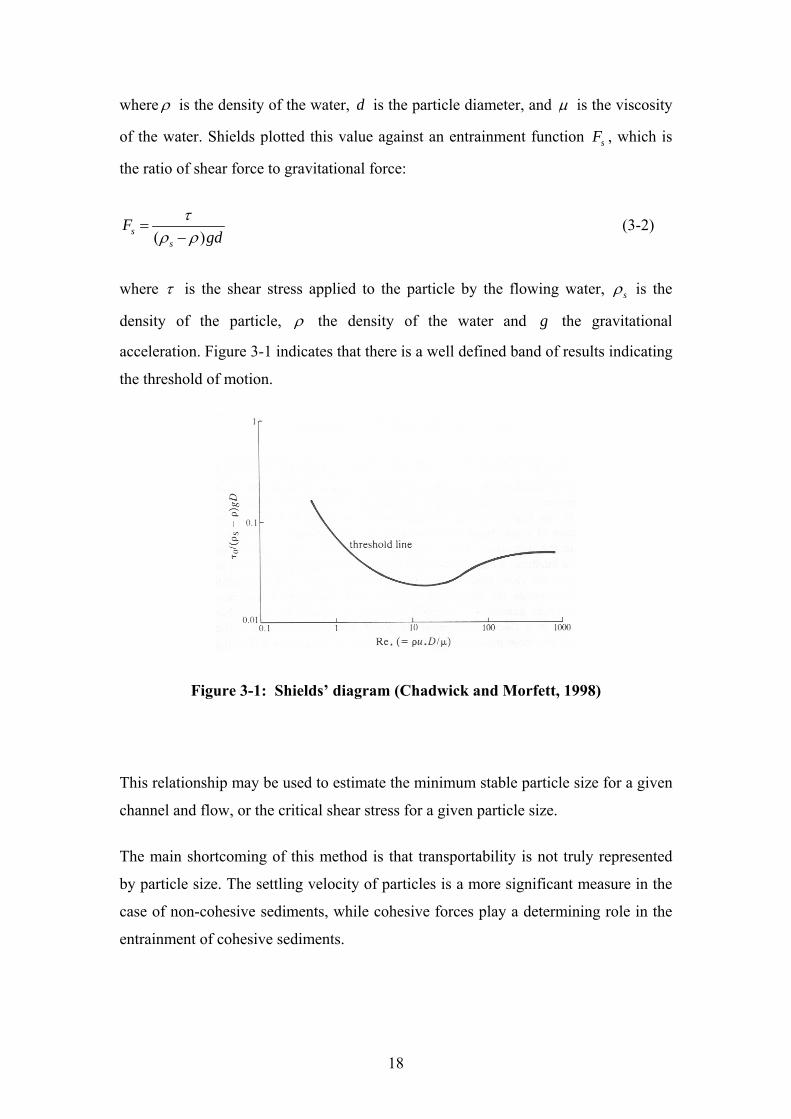
where ρ is the density of the water, d is the particle diameter, and μ is the viscosity

of the water. Shields plotted this value against an entrainment function sF , which is

the ratio of shear force to gravitational force:

( )ss

Fgd

τρ ρ

=−

(3-2)

where τ is the shear stress applied to the particle by the flowing water, sρ is the

density of the particle, ρ the density of the water and g the gravitational

acceleration. Figure 3-1 indicates that there is a well defined band of results indicating

the threshold of motion.

Figure 3-1: Shields’ diagram (Chadwick and Morfett, 1998)

This relationship may be used to estimate the minimum stable particle size for a given

channel and flow, or the critical shear stress for a given particle size.

The main shortcoming of this method is that transportability is not truly represented

by particle size. The settling velocity of particles is a more significant measure in the

case of non-cohesive sediments, while cohesive forces play a determining role in the

entrainment of cohesive sediments.

19

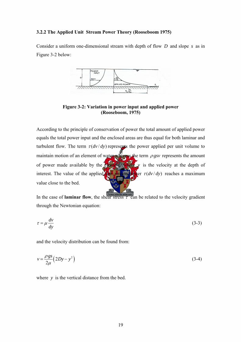
3.2.2 The Applied Unit Stream Power Theory (Rooseboom 1975)

Consider a uniform one-dimensional stream with depth of flow D and slope s as in

Figure 3-2 below:

Figure 3-2: Variation in power input and applied power (Rooseboom, 1975)

According to the principle of conservation of power the total amount of applied power

equals the total power input and the enclosed areas are thus equal for both laminar and

turbulent flow. The term ( / )dv dyτ represents the power applied per unit volume to

maintain motion of an element of water whereas the term gsvρ represents the amount

of power made available by the element, where v is the velocity at the depth of

interest. The value of the applied unit stream power ( / )dv dyτ reaches a maximum

value close to the bed.

In the case of laminar flow, the shear stress τ can be related to the velocity gradient

through the Newtonian equation:

dvdy

τ μ= (3-3)

and the velocity distribution can be found from:

( )222gsv Dy yρμ

= − (3-4)

where y is the vertical distance from the bed.

20

In the case of turbulent flow, the shear stress is given by:

22

dvldy

τ ρ⎛ ⎞

= ⎜ ⎟⎝ ⎠

(3-5)

where l is the mixing length expressed as l yκ= where κ is the Von Karman

dimensionless constant (equal to 0.4). The velocity at a vertical distance y from the

bed for turbulent flow is given by the log-deficiency equation:

0

2 .ln ygDsy

v π⎛ ⎞⎜ ⎟⎝ ⎠

= (3-6)

where 0y is the distance from the bed at which the velocity is mathematically zero,

found by:

00 14.8 29.6

sR ky ≈ ≈ (3-7)

0R is the radius of the eddies formed against the bed and sk is the absolute roughness

of the bed.

In turbulent flow it is not possible for turbulent fluid layers to slide over one another

as in the case of laminar flow. A thin sectional element over the depth of the fluid

therefore has to move as a unit. Since the velocity near the bed equals zero, the only

means of movement is through rotation of the element around a point near the bed.

Fluid movement in a canal is translational and such movement is only possible if there

is a rotation centre point that also translates.

According to the concept of least applied power, flow near a boundary will be either

turbulent or laminar, depending upon which type of flow requires the smallest amount

of power per unit volume, ( / )dv dyτ to maintain it. This means that where the two

alternative modes of flow exist, there will be a laminar sublayer next to a smooth

boundary below the turbulent flow zone.

21

By setting the applied stream power of laminar and turbulent flows equal for a given

value of τ , the distance 1y of this rotational point from the bed, is found by:

12 .vygDsπ

= (3-8)

This is also the depth of the transition between laminar and turbulent flow. At this

level the velocity of laminar flow would be:

2v gDsπ= (3-9)

which is the required translatory velocity of the centre of rotation for turbulent flow.

3.2.3 Incipient Motion Criteria with the Stream Power Theory (Rooseboom, 1992)

For non-cohesive sediments, incipient motion is determined according to the sediment

transport model used. The power approach provides us with the ability to define both

the transporting capacity of a stream and the effort required to transport material in

directly comparable terms.

Critical Conditions for Cohesionless Sediment

The applied power required per unit volume to suspend a particle with density sρ and

settling velocity, w , in a fluid with density ρ equals:

( )sdv gwdy

τ ρ ρ⎛ ⎞

= −⎜ ⎟⎝ ⎠ (3-10)

where

12( )s

d

gdwC

ρ ρρ

⎡ ⎤−∝ ⎢ ⎥⎣ ⎦

(3-11)

22

For rough turbulent conditions, the value of the applied unit stream power to maintain

motion along the bed is:

gsD gDsdvdy d

ρτ⎛ ⎞

=⎜ ⎟⎝ ⎠

(3-12)

Setting these two equations equal, and assuming that the value of the drag coefficient

dC for determining w is a constant (which is true for large diameters), then the

condition of incipient motion under rough turbulent flow conditions is given by:

constant 0.12gDsw

= = (3-13)

For smaller particles where the value of .

13gDs d

v< the relationship for incipient

motion is found to be:

1.6.

gDsw gDs d

v

= (3-14)

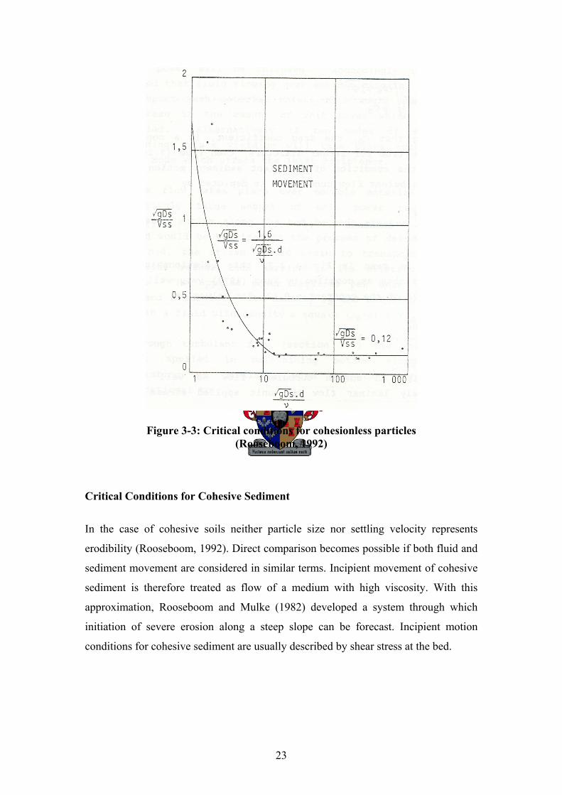
Figure 3-3 shows the critical conditions for cohesionless sediment particles according

to the applied stream power principle. Note that Vss in Figure 3-3 equals w , the

settling velocity.

23

Figure 3-3: Critical conditions for cohesionless particles (Rooseboom, 1992)

Critical Conditions for Cohesive Sediment

In the case of cohesive soils neither particle size nor settling velocity represents

erodibility (Rooseboom, 1992). Direct comparison becomes possible if both fluid and

sediment movement are considered in similar terms. Incipient movement of cohesive

sediment is therefore treated as flow of a medium with high viscosity. With this

approximation, Rooseboom and Mulke (1982) developed a system through which

initiation of severe erosion along a steep slope can be forecast. Incipient motion

conditions for cohesive sediment are usually described by shear stress at the bed.

24

In the MIKE 21C software that will be used to model the transport of fine sediment in

this research, a critical shear stress for erosion is specified. Erosion will commence at

a rate of erosion, E, as soon as the bed shear stress exceeds this value, according to the

erosion function:

0 1 , > m

cece

E E τ τ ττ⎛ ⎞

= −⎜ ⎟⎝ ⎠

(3-15)

where 0E and m are the dimensionless coefficient and exponent and ceτ is the user

specified critical shear stress for erosion. Very little information is available on

estimating a value for this parameter. The higher the percentage of fine material on

the bed, the higher stresses will be required to erode the bed because of the

cohesiveness. Throughout this research, a critical shear stress value of 1.04 N/m2 is

used for a cohesive bed.

3.2.4 Suspended Load and Bed Load

If water is flowing, it can carry suspended particles. The settling velocity of a

suspended particle, w, is given by Stoke's Law (Chadwick and Morfett, 1998):

2( )18

s gdw ρ ρμ

−= (3-16)

As there will always be a range of different particle sizes in the flow, some will have

sufficiently large diameters that they settle on the river or stream bed, but still move

downstream. This is known as bed load and the particles are transported via

mechanisms such as saltation, rolling and sliding.

25

3.3 Traditional Equilibrium Sediment Transport Theories

Equilibrium in this case refers to actual sediment transport being equal to the transport

capacity at a section. This is a realistic approach only when coarse sediments are

transported without any constraints of sediment availability.

These sediment transport equations have thus been tested and calibrated for sand

transport only and not for fine sediment. These equations basically consists of two

groups: the equations that predict bed load and suspended load separately and those

that predict a total sediment load. Traditionally, the equations of hydraulics and

sediment transport are based on the conservation of mass, energy and momentum.

Most of these are for river applications and not for reservoir applications. Four

existing theories are presented in the following paragraphs as described by Basson

and Rooseboom (1997):

a) Engelund and Hansen (1967)

Engelund and Hansen related input power per unit area of channel boundary to

sediment discharge using dimensional analysis and proposed the following

relationship:

5/ 22

2 0.1gDsv

φ θ= ⋅ (3-17)

The Engelund and Hansen coefficients,φ and θ , are described by:

3

s

s

Q

gd

φγ γγ

=⎛ ⎞−⎜ ⎟⎝ ⎠

and ( )s

gDsd

ρθγ γ

=−

The total sediment discharge in then given by:

( )

5/ 22

3

20s

ss

v gDsQ gdgDs d

γ γ ργ γ γ

⎛ ⎞⎛ ⎞−= ⋅⎜ ⎟⎜ ⎟ ⎜ ⎟−⎝ ⎠ ⎝ ⎠

(3-18)

26

where:

D = Flow depth g = Gravitational acceleration v = Flow velocity s = Slope

sQ = Total sediment discharge γ = Specific weight of water

sγ = Specific weight of sediment d = sediment diameter

b) Ackers and White (1973)

Also by using dimensional analysis, Ackers and White derived an equation

representing total sediment discharge in terms of three dimensionless numbers; a

sediment transport function grG , a mobility number grF and a dimensionless sediment

particle size grd :

'' 1/

nmgr

grs

F gDsc DG cA d vγ γ

⎛ ⎞⎛ ⎞= − = ⎜ ⎟⎜ ⎟ ⎜ ⎟⎝ ⎠ ⎝ ⎠

(3-19)

( )( )

1

32 log(10 / )/ 1

n n

grs

gDs vFD dgd γ γ

−⎛ ⎞

= ⎜ ⎟− ⎝ ⎠

(3-20)

( ) 1/3

2

/ 1sgr

gd

γ γυ

⎛ ⎞−= ⎜ ⎟⎝ ⎠

(3-21)

where υ = kinematic viscosity, equal to 10-6 m2/s. The coefficients 'c , A , m and n

are functions of sediment particle size and have the following values for coarse

sediment where grd > 60: n =0, A =0.170, m =1.50 and 'c =0.025. For values of grd <

60, their values are given by these equations:

1 0.56 log( )grn d= − ⋅ , 0.23 0.14gr

Ad

= + , 9.66 1.34gr

md

= + and

2log ' 2.86 log( ) log ( ) 3.53gr grc d d= ⋅ − −

27

c) Van Rijn (1984)

In this transport model the sediment load is divided between bed load and suspended

load according to the relative magnitudes of the bed shear velocity, and the particle

falling velocity. When the bed shear velocity exceeds the falling velocity, sediment is

transported as both suspended and bed load.

Van Rijn Bed Load

Bed load is considered to be transported by rolling and saltation and the rate is

described as a function of saltation height. The reference concentration is determined

from the bed load transport. Bed load is computed from the product of particle

velocity, bsu , saltation height, bδ , and the bed load concentration, bC :

b bs b bq u Cδ= (3-22)

Expressions for the particle velocity and saltation height were obtained by numerical

solving of the equations of motion applied to a solitary particle. These expressions are

given in terms of two dimensionless parameters which are considered to adequately

describe bed load transport; a dimensionless particle diameter, *D , and a transport

stage parameter, T , as defined below:

1/ 3

* 50 2

( 1)sD d gv−⎡ ⎤= ⎢ ⎥⎣ ⎦

(3-23)

( ) ( )( )

2 2

,2

,

g f cr

f cr

u uT

u

−= (3.24)

where gu is the bed shear velocity, related to grains, u is the mean flow velocity, ,f cru

is the Shields critical bed shear velocity and 50d is the median particle diameter. gu is

the effective bed shear and is so defined in order to eliminate the influence of bed

forms since form drag was not considered to contribute to bed load transport.

28

Extensive analysis of flume measurements of bed load transport yielded the following

expression for the bed load concentration:

0*

0.18bTC CD

= (3.25)

where 0C is the maximum bed concentration.

Combining equations for particle mobility and saltation height with equation 3.25

gives the following expression for bed load transport, bq , valid for particles in the

range of 0.2mm to 2.0mm.

2.13500.3

*

0.053 ( 1)bTq s gd

D⋅

= − (3.26)

Van Rijn Suspended Load

The suspended load is determined from the depth-integration of the product of the

local concentration and flow velocity. The suspended load method is based on the

computation of a reference concentration determined from the bed load transport, thus

the reference concentration, aC , is described as a function of *D and T .

1.550

0.3*

0.015ad TCaD

= (3.27)

where the reference level, a, at which the bed concentration is determined is given by:

50

0.01max

2h

ad

⎛ ⎞= ⎜ ⎟

⎝ ⎠

where h is the water depth.

Van Rijn (1984) derived the following expression for the suspended load:

s aq FuDC= (3.28)

29

in which [ ]

' 1.2

'

1 1.2 '

z

Z

a aD DF

a ZD

⎡ ⎤ ⎡ ⎤−⎢ ⎥ ⎢ ⎥⎣ ⎦ ⎣ ⎦=⎡ ⎤− −⎢ ⎥⎣ ⎦

(3.29)

where the modified Rouse suspension number is given by 'Z z ψ= + , and the

correction factor, ψ , is given by: 0.8 0.4

0

2.5 a

g

Cwu C

ψ⎡ ⎤ ⎡ ⎤

= ⎢ ⎥ ⎢ ⎥⎢ ⎥ ⎣ ⎦⎣ ⎦

for values of ψ between

0.1 and 1.0 with z the Rouse suspension parameter and ug the bed shear velocity.

The Van Rijn equations are based on several empirical relationships and draws the

distinction between bed load and suspended transport which cannot be justified from

fundamental theory. The equations do however provide for changes in bed roughness

and energy dissipation for different flow regimes and sediment transport modes.

d) Unit (input) stream power (Yang, 1973, Rooseboom, 1975)

The basic principles of this approach were proven in South Africa in 1974 and has

since been used in the planning and design of various reservoir sedimentation studies.

Rooseboom (1975) found that the suspension theory (Rouse, 1937) can be used to

describe both bed and suspended load and the incipient motion criteria, and is

therefore well suited to analysis of total carrying capacity.

Sediment transport capacity per unit width in terms of flow parameters can be

calculated if it is assumed that sediment particles are transported at the same velocity

as the fluid:

0

D

s yq Cv dy= ⋅∫ (3-30)

where:

zdvCdy

τ⎛ ⎞

∝ ⎜ ⎟⎝ ⎠

and dvdy

τ the applied power,:

30

C = Sediment concentration τ = Bed shear stress w = Settling velocity κ = Von Karman coefficient

wzgDsκ

= is the suspension theory coefficient and 0y the distance from the bed

where v = 0 mathematically, which after integration leads to an equation of the form

(Rooseboom, 1975):

( ) 1

1 2 01

0

log log log2

sz

q Cvsq sD gDs

y

α ααπ

⎛ ⎞⎜ ⎟⎜ ⎟

= + ⎜ ⎟⎜ ⎟⎜ ⎟⎜ ⎟⎝ ⎠

(3-31)

where:

1α , 2α = Coefficients

1z = The suspension theory coefficient as derived by Rooseboom (1975)

0C = Sediment concentration at the bed where v = 0 at y = 0y

v = Average flow velocity

Yang (1972) found that equation 3-31 described sediment transporting capacity

particularly well. Yang used a slightly different approach by including a critical

stream power value for incipient motion in equation 3-32 below. The equation by

Yang was, however, only calibrated with laboratory data.

3 4log log( )scr

q vs vsq

α α⎛ ⎞

= + ⋅ −⎜ ⎟⎝ ⎠

(3-32)

with 3α , 4α a constant and coefficient, crvs the critical input stream power for

incipient motion. Yang (1973) then also defined sediment transport capacity in terms

of the settling velocity, w:

5 6log logs crq vs vsq w

α α⎛ ⎞⎛ ⎞ −

= + ⋅ ⎜ ⎟⎜ ⎟⎝ ⎠ ⎝ ⎠

(3-33)

31

with 5α and 6α the constant and coefficient respectively and w the settling velocity.

The last term in equation 3-31 was found not to vary considerably and can be equated

to the 5α coefficient of Yang.

In 1984, Yang proposed a gravel transport equation with an incipient motion term.

The maximum sediment transport capacity of a stream can therefore be determined by

an equation of the type:

log logsq vsq

α β= ⋅ + (3-34)

where vs represents the average input unit stream power at a cross-section in a

reservoir or river, and α = coefficient and β = constant.

3.4 Non-equilibrium Sediment Transport

3.4.1 Cohesive Sediment

Cohesive sediments are very fine (d < 0.065mm) negatively charged clay minerals

which have a certain capacity to absorb cations. Small particles (d < 0.002mm) can

remain in colloidal suspension for a long time because of the repulsive magnetic

forces between them. Cohesive sediments are normally transported as suspended load.

Deposits of cohesive sediment are held together by the bonding force of positive and

negative ionic charges of the clay minerals. Cohesive sediments are characterized by

two main properties: plasticity and cohesion, due to surface physico-chemical forces

on the sediment particles smaller than 2 microns. Under the influence of these and

fluvial conditions, colliding fine particles stick to each other forming agglomerations

known as flocks, with sizes and settling velocities exceeding by orders of magnitude

those of the individual particles.

The boundary between cohesive and cohesionless sediment is not clearly defined and

generally varies with the type of sediment. Dominance of interparticle cohesion over

32

gravitational force increases with decreasing particle size. Thus the effect of cohesion

on the behaviour of clays (< 0.004mm) is much more pronounced than on silts (0.004-

0.065mm). Beck and Basson (2003) found that with as little as 7% clay and silt in

sediment mixtures the sediments will effectively have the properties of cohesive

sediments. For reservoir conditions, it is of utmost importance to forecast the transport

of fine sediments (silt and clay), since in most South African impoundments they

form the main sediment body. In practice, the prediction of the transport of fine

sediments within reservoirs is based on different approaches:

Use of the diffusion equation by Zhang (1980) as discussed in section 3.4.3

Use of the equilibrium sediment transport equations which were recalibration

with fine sediment transport data

Combinations of sediment transport equations for sand fractions and diffusion

equations for fine sediments

Use of computational models such as DHI’s 2-dimensional MIKE 21C with an

advection-dispersion model for the transport of fine sediment.

3.4.2 Non-equilibrium Sediment Transport Background

With the equilibrium transport equations, a state of sediment equilibrium is reached

within each time step of the calculation. Equilibrium refers to actual sediment

transport being equal to the transport capacity at a section. It is assumed that the

sediment load at the next section is equal to the capacity at that section for the same

time-step and that the difference in sediment between the two sections will either

deposit or erode during that time-step. This assumption is called instantaneous

adaptation and is only valid for the transport of coarse sediment.

With fine sediments, however, the adjustment to the saturated sediment transport

capacity is not instantaneous and time and distance lags are associated with the

change in sediment transport, until equilibrium is reached. This lag, often called

“adaptation length”, is due to the extremely small settling velocities of the fine

sediments (Basson and Rooseboom, 1997).

33

Two types of non-equilibrium sediment transport modes can be identified (Batuca and

Jordaan, 2000):

Undersaturated transport occurs when the availability of the sediment from

surface erosion is limited and the actual sediment concentration is less than the

transport capacity.

Oversaturated transport occurs as the sediment concentration exceeds the

transport capacity. Adaptation lengths can even be longer than the reservoir

itself in the case of very fine sediments in deep reservoirs.

3.4.3 Non-equilibrium Sediment Transport Theories for Steady Flow (Rooseboom and Basson, 1997)

a) Mehta and Partheniades (1973) showed that suspended sediment concentration in

reservoirs diminishes rapidly from an initial value, oC , to a constant equilibrium

concentration value, eqC . The value of eqC decreases with decreasing bed shear stress,

τ , becoming zero at a threshold value of minbτ . It was shown that the ratio of relative

equilibrium concentration, * /eq eq oC C C= , remained constant, independent of the

initial concentration, oC , but dependant on the bed shear stress, τ .

This adjustment to a single equilibrium concentration is attributed to the adjustment of

the stream power to minimize energy dissipation. This equilibrium is not the

maximum equilibrium sediment transport, but rather an undersaturated transport due

to limited sediment availability.

b) Han and He (1990) calibrated non-equilibrium equations with field data and

established criteria for non-equilibrium sediment transport calibration coefficients for

rivers and reservoirs. Most of these equations have the format of a steady advection-

dispersion equation.

34

Sediment transport estimations were until recently done by using an equilibrium

transport equation, although sediment transport is often in non-equilibrium.

Equilibrium formulae based on uniform flow experiments in hydraulic laboratories

are no longer considered as a satisfactory component of a mobile-bed modelling

system. Time and space lags between actual and equilibrium transported sediment

load should therefore be considered (Cunge, 1989).

c) Zhang (1980) found the basic equation of 2D diffusion to be of the form:

2

2

C C Cv wx z z

∂ ∂ ∂=∈ +

∂ ∂ ∂ (3-35)

with:

C = Sediment concentration ∈ = Coefficient of turbulent exchange w = Settling velocity of sediment particles v = Flow velocity

Zhang determined the analytical solution for deposition as:

( ) ( ) /cp

Kp Cp

dC xw C C x q

dx⎡ ⎤= ∝ −⎣ ⎦ (3-36)

with the following boundary conditions:

at the water surface: , 0Cz D wCz

∂= ∈ + =

∂

on the reservoir bed: ,00, constantKC wz Cz

∂= = − =

∂ ∈

at the entrance to the reservoir: 00, C = C ( )x f z= ⋅

By substituting initial conditions, 00, ( )cpx C x C= = , the final expression of the rate

of change in sediment concentration along the reservoir is:

( / )

0( )wx qs st s stq q e q q−∝= + − (3-37)

35

with:

sq = Sediment discharge per unit width at the exit

stq = Sediment carrying capacity

0sq = Sediment discharge per unit width at the entrance In the case of erosion, the same equation can be derived:

( / )

0( )wx qs st s stq q e q q−∝= + − (3-38)

If ( / )wx qeξ −∝= denotes sediment transport under non-equilibrium conditions, the final

expression for ξ , with the inclusion of the empirical coefficients ( 3 4 5, and K K K )

reads:

For deposition: 41 3exp ( (0.41 0.77 / ) ( / ))KK C gC x qξ = − − ⋅ (3-39)

For erosion: 0.3 0.52 5exp ( ( / ))K Q s x qξ = − ⋅ (3-40)

d) Soares (1982) derived equations for non-equilibrium suspended sediment

transport, similar to those of Zhang (1980). The mass balance of sediment of a given

size jd is:

( )j

j jd e

CQ x q q T xx

⎛ ⎞∂Δ = − + Δ⎜ ⎟∂⎝ ⎠

(3-41)

jdq , j

eq = Fluxes of deposition and erosion of sediment Q = Flow rate T = Width

( Ct

∂∂

is neglected in this equation)

36

Let * jCT = average concentration of sediment transporting capacity, then if *1 (deposition)j j

i iCT CT +> , the rate of deposition:

*( )j j j

d jq w C CT= − − and equation 3-41 becomes:

*( ) /j

j jj

C w C CT T Qx

∂= − −

∂ (3-42)

Integrating between two sections:

*

1 1( ) exp ( / )j ji i i jC C CT w xT Q+ += − − Δ (3-43)

if *1

ji iC CT +≤ (erosion will occur depending on the availability of sediment of the

given size, jd , on the stream bed.

The rate of erosion: ( )j j je bq C Cλ= − (3-44)

Erosion is proportional to the difference between the availability on the bed and the

concentration carried by the flow. Although erosion is dominant, deposition will still

occur at rate jjw C and equation 3-41 becomes:

( ) ( )j

jj jb j j

j j

C TC C wx w Q

λλ

λ∂

= − − +∂ +

(3-45)

Integration of equation 3-45 between sections i and 1i + yields:

( )1 exp j jj j j ji i b j j b

j j j j

T xC C C w Cw Q w

λ λλ

λ λ+

⎛ ⎞ ⎡ ⎤Δ= − − + +⎜ ⎟ ⎢ ⎥⎜ ⎟+ +⎣ ⎦⎝ ⎠

(3-46)

When x is large, flow in section ( 1i + ) will approach it’s transport capacity *1

jiCT + :

37

*1

jj ji b

j j

CT Cw

λλ+ =

+ (3-47)

and the final equation is:

* *1 1 1( ) exp ( )j j j j

i i i i j jT xC CT C CT w

Qλ+ + +

⎡ ⎤Δ= + − − +⎢ ⎥

⎣ ⎦ (3-48)

which is similar to the equations presented by Karanshev (1963) and Zhang (1980).

e) Di Silvio (1995) proposed the use of the following non-equilibrium transport

equation:

**

1 ( )i

ii ci i

C C Cx L

β∂= −

∂ (3-49)

where:

iC = the actual sediment transport per fraction

iβ = the percentage of i-th fraction in the bed composition *i

L = the adaptation length for each fraction *ciC = the transport capacity of the i-th fraction

For fine particles, * /i iL vD w→ , which means that the adaptation length of silt and

clay may be even larger than the length of the reservoir.

All the non-equilibrium sediment transport theories and equations that have been

discussed in the preceding paragraphs were derived for steady flow conditions.

Reservoir sedimentation processes are highly dynamic and it has therefore been

decided to describe them by using an unsteady advection-dispersion equation.

38

3.5 Advection and Dispersion

Terminology on the subject of advection and dispersion frequently differs from

engineering to chemical and geological literature. For the remainder of this research,

the processes of advection and dispersion will be defined as follows:

When a fluid of higher sediment concentration is injected at a point into a turbulent

flow it will be subjected to two distinct processes: (a) it will be swept along

(advected) with a velocity comparable to that of the flow and (b) it will be mixed

(diffused) due to turbulence and molecular diffusion. Diffusion due to turbulence is

normally two or more orders of magnitude larger than molecular diffusion, so the

latter will be omitted from further consideration. Dispersion is then the combination

of advection and diffusion (Chadwick and Morfett, 1998).

The 1D unsteady advection-dispersion equation has the following form (Basson and

Rooseboom, 1997):

2

2

C C Cu D sst x x

δ δ δδ δ δ

+ − = (3-50)

where:

D = The one-dimensional dispersion coefficient u = Flow velocity t = Time x = Distance in the direction of flow The source/sink (ss) term represents the increase in suspended sediment concentration

as a result of erosion and also the decrease in the concentration due to deposition of

the suspended sediment.

In the case of non-cohesive sediments the source/sink term is represented by:

*( )C CssaT−

= (3-51)

39

where:

*C = The equilibrium sediment transport calculated with a sediment transport

formula T = The time scale defined as settling time (water depth divided by settling velocity) a = A calibration parameter and can be interpreted as a mean settling depth

Basson and Rooseboom (1997) used suspended sediment concentration data from a

series of channel tests to calibrate the parameter a for non-equilibrium transport of

sediments using the MIKE 11 software for one-dimensional modelling. Thereby

certain value ranges for a were established for the finer fractions of various sediment

types.

For cohesive sediment fractions the source/sink term should be represented by:

0 ; cess τ τ= < (No erosion)

1 ; m

ce cmece

ss E τ τ τ ττ⎛ ⎞

= − < <⎜ ⎟⎝ ⎠

(Surface erosion)

( )*

; cme

C Css

tτ τ

−= >

Δ (Mass erosion, no lag)

where:

τ = Bed shear stress ceτ = Critical shear stress for erosion

cmeτ = Critical shear stress for mass erosion E = Erosion rate

The source/sink term usually includes a deposition function that is implemented once

the bed shear stress has exceeded the critical shear stress for deposition, deτ (DHI,

2003):

40

1scd

D w c ττ

⎛ ⎞= −⎜ ⎟

⎝ ⎠ , cdτ τ< (3-52)

where:

sw = Settling velocity cdτ = Critical shear stress for deposition

c = Concentration 3.6 Integrated Mathematical Modelling of Unsteady Flow, Suspended Sediment

Transport and Morphological Change

3.6.1 Background

Reservoir sedimentation and morphological processes are amongst the most complex

and least understood phenomena in nature. In early times, the sedimentation research

methodologies were primarily based on field observation and physical modelling.

This chapter is focused on the methodologies of mathematical modelling, more

precisely numerical-empirical modelling which is sometimes referred to as

computational modelling. Although sedimentation, as a science, only has a sixty-year

history and some of the fundamental problems are still unclear, it is nevertheless

possible to predict sediment transport through mathematical modelling (Wang and

Wu, 2004).

The initial attempts in application of mathematical models in conjunction with

empirical functions obtained from laboratory experiments to the investigation of river

sedimentation and morphological processes can be found in the 1950’s.

The basic equation for non-equilibrium sediment transport was first obtained by Dou

(1963) using a heuristic approach in his study of tidal flows. It was later elaborated

and derived mathematically by Han (1980), Lin and Shen (1984) and Lin et al. (1983)

for both 1D and 2D cases.

41

The three-dimensional transport of suspended sediment is governed by the equation

(Zhou et al. 2004):

3

( 1, 2,3) i si i i

c c cu c v w it x x x x∂ ∂ ∂ ∂ ∂

+ − = =∂ ∂ ∂ ∂ ∂

(3-53)

where c is the sediment concentration, xi the spatial coordinates, ui the flow velocities,

vs the coefficients of diffusion, w the settling velocity of sediment particles and t the

time duration. The transport equation for one- and two-dimensional problems may be

obtained by integrating equation 3.53 over a cross-section (1D) or a depth (2D) with

suitable conditions imposed at the loose bed. Thus the following depth- and section-

integrated equations are obtained for 2D and 1D cases, respectively (Zhou and Lin,

1998):

2D) ( 1, 2)( )

i

i

U CC w it x h C

αφ

∂∂+ = − =

∂ ∂ − (3-54)

1D) 1

( )s sS S wV St x D

β α∂ ∂+ = − −Φ

∂ ∂ (3-55)

where C and U are respectively the depth-averaged sediment concentration and flow-

velocity, S the section-averaged sediment concentration, V the section-averaged flow

velocity and, h the depth of flow for the 2D case. D the section-averaged depth of

water for the 1D case, and φ and Φ the depth–integrated and section averaged

transport capacities, respectively. Falconer and Owens (1990) defined the adjustment

coefficient as the ratio of the bed layer concentration to the depth-averaged

concentration; /ac Cα = .

Equation 3.53 is free from any empirical parameters. The equations for 2D and 1D

cases however contain parameters α , φ and Φ that must be determined before these

equations may be solved. For 3D computations, properly imposed boundary

conditions over the bed must be given. There are several possible ways to accomplish

this. For example, one may adopt the concentration at a reference level (Dirichlet

42

condition), or a gradient bed layer concentration (Neumann condition), or a

combination of the two (mixed condition) (Zhou et al., 2004)

This branch of research was intensified and broadened in the 1970’s. Since then a

number of 1D models (eg. Cunge et al.,1980; Thomas, 1982; Rahuel and Holly, 1989;

Wu and Vieira, 2002) were applied to sedimentation studies in rivers and reservoirs.

More recently, numerous 2D and 3D numerical-empirical (eg. Sheng, 1983; Wang

and Adeff, 1986; Spasojevic and Holly, 1993; Jia and Wang, 1999; Wu et al., 2000)

have been developed to simulate sediment transport processes and morphological

changes in channels with mobile bed and banks, both in the laboratory and in nature.

In the early development stage, the sediment transport model only considered either

bed load or suspended load with a single representative size. Realistically, sediments

in rivers are often heterogeneous (non-uniform) in size, not to mention that they have

variable shape and density. Furthermore, the transport mode changes from bed load to

suspended load and vice versa with flow conditions.

Traditionally, the transport of sediment, especially bed load, was simulated based on

the assumption of local instantaneous equilibrium. Due to the observed spatial and

temporal lags between the sediment motion and water flow, it was found that the

traditional equilibrium transport models need to be improved to take into account the

non-equilibrium features of sediment transport, especially under unsteady flow

conditions (Wang and Wu, 2004).

To meet the needs in engineering practice, the capability of river and reservoir

sedimentation modelling have been further advanced remarkably in recent years.

Many established models are capable of simulating non-cohesive and cohesive

sediment transport, local scouring, channel widening and meandering.

43

3.6.2 Mathematical Model Assumptions

The phenomena of flow and sediment transport in rivers are characterised by

turbulence, free-surface variation, bed change, phase interaction, etc. A model capable

of including all of these effects accurately has yet to be developed. At the present,

most sediment transport models have adopted the following assumptions (Wang and

Wu, 2004):

Sediment concentration is so low that the interaction between flow and

sediment movement can be neglected. Therefore, the clear-water flow and the

sediment transport equations can be solved separately.

Bed change is much slower than flow movement. Therefore, at each time-step

the flow can be calculated assuming a “fixed” bed.

The hiding and exposure mechanism in bed material is considered through the

introduction of correction factors in the non-uniform sediment transport

capacity formulas. The interactions among different size classes of moving

sediment are ignored. Thus the transport of each size class of sediment can be

handled individually.

Based upon the above assumptions, 1D, 2D and 3D governing equations of flow,

sediment transport and morphological changes have been developed. These equations

will be discussed in detail in the following sections.

3.6.3 One-dimensional Mathematical Modelling

One-dimensional models are mostly used in river and reservoir applications around

the world, although computationally “heavy” two-dimensional and even 3D models

have been developed. With 1D modelling, conditions are averaged over the width and

depth, so that variations are limited to the x direction i.e. the direction of the mean

velocity of flow. It must be emphasized that the concentration is assumed to be fully

mixed over the cross section.

44

With laterally integrated 1D models, the shallow water flow is governed by the well-

known St.Venant equations. The sediment transport can be separated as bed load and

suspended load according to sediment transport models. The governing equation for

the non-equilibrium transport of non-uniform sediments is (Wang and Wu, 2004):

( )*( ) 1 ( 1, 2,..., )tk tk

tk t k lks

AC Q Q Q q k Nt x L

∂ ∂+ + − = =

∂ ∂ (3-56)

where:

t = Time A= Flow cross-section x = Longitudinal coordinate

tkC = Section averaged sediment concentration

tkQ = Actual sediment transport rate

*t kQ = Sediment transport capacity or the so-called equilibrium transport rate

sL = Non-equilibrium adaptation length

lkq = Side inflow or outflow sediment discharge from bank or tributary streams per unit channel length k = Representative sediment size class N= Total number of size classes This equation can be applied to bed load or suspended load depending on how the

sediment transport rate and the adaptation length are defined. For example,

defining * */( ), and s sk tk tk tk tkL Uh w Q QC Q QCα= = = , one can rewrite equation 3-56

as the commonly used suspended load transport equation with the exchange term

*( )sk tk tkw C Cα − . Here, U is the section averaged velocity, h is the flow depth, wsk is

the settling velocity of sediment particles, α is the non-equilibrium adaptation or

recovery coefficient, and *tkC is the suspended load transport capacity. When equation

3-56 is applied to the bed load, the transport rate tkQ is the sum of bed load and

suspended load transport rates. The bed deformation due to size class k is determined

by means of:

*1(1 ') ( ) ( 1, 2,..., )b

tk tkk s

Ap Q Q k Nt L

∂⎛ ⎞− = − =⎜ ⎟∂⎝ ⎠ (3-57)

45

where 'p is the bed material porosity and ( / )bA t∂ ∂ is the bed deformation rate caused

by size class k. Combining equations 3-56 and 3-57 leads to the sediment continuity

equation, which could also be used to calculate the bed deformation.

It should be noted that as the sediment size increases, the adaptation length sL

reduces. As a result, the exchange term becomes dominant in equation 3-56. In such a

case, equation 3-56 reduces to *tk tkQ Q= , which is the traditional assumption of local

equilibrium. Therefore, the equilibrium sediment transport model is a special case of

the non-equilibrium transport model.

The sediment transport capacity can be written in a general form as:

*

*tk bk tkQ p Q= (3-58) where bkp is the availability factor of sediment, which is defined here as the bed

material gradation in the mixing layer and *tkQ is the potential sediment transport

capacity for size class k, which can be determined with the help of empirical

relationships.

3.6.4 The Non-equilibrium Adaptation Length The non-equilibrium adaptation length Ls, which characterises the distance required

for sediment to adjust from a non-equilibrium state to an equilibrium state, is a very

important parameter in the non-equilibrium transport model. Traditionally, the non-

equilibrium adaptation length of suspended load is given with /( )s skL Uh wα= .The

coefficient α can be calculated with the method of Armanini and Di Silvio (1988) or

other semi-empirical methods. Values of α calculated from these methods are usually

larger than 1. However, in practice, α has been given different values by many

researchers, most of them being less than 1. It has been suggested that α =1 for the

case of strong erosion, α = 0.25 for strong deposition and α = 0.5 for weak deposition

and erosion (Wang and Wu, 2004).

46

3.6.5 One-dimensional RESSASS Model: Tarbela Reservoir, Pakistan

(HR Wallingford, 1998)

a) Background

Tarbela Dam was built between 1970 and 1975 and is located on the Indus River. The

dam is vital to Pakistan’s economy as it provides 40% of the country’s water storage,

crucially important for irrigation during the dry season, and 35% of the country’s

energy requirements from hydroelectric generation. About 25% of the original live

storage had been lost and the sediment delta was approaching the dam by 1997.

b) Description of the Model

The mathematical model RESSASS of HR Wallingford was used to simulate reservoir

sedimentation in Tarbela Reservoir. The model is one-dimensional in the sense that all

hydraulic variables are considered constant at any cross-section at any particular time.

The model is based on the equations that describe flow and sediment movement.

Within the model, sediment transport calculations are carried out for a range of

different sediment sizes. The model is a time-stepping one, that is, initial conditions

are input to equations which predict water levels and bed levels a short time later,

typically one day. These predictions then provide the input conditions for the next

time step. The process is repeated many times to make predictions over the required

time period. Cross-sections are used to specify the geometry of the reservoir. The

model then predicts revised bed levels and the location and composition of sediment

deposits.

The model runs on a 60 year sequence of sediment and water inflows. The sequence

consists of the 1967 to 1996 inflows to Tarbela repeated once to give the required 60

year sequence. The inflows are based on the flow records at Besham Qila, located

upstream of the reservoir. The sediment inflows were calculated using the sediment

rating equation on these inflows together with the Ackers and White equation. For the

model verification runs, the model water levels were matched to the observed levels

since the first impoundment of the reservoir.

47

The model operates with the following boundary conditions:

Variations of incoming flow with time

Corresponding variations of incoming sediments with time

Variations of water level at the dam as defined by the operating policy

This means that, at any particular time, the model computes the outflow through the

dam (the model does not take into account where that outflow occurs or whether the

infrastructure at Tarbela is capable of delivering that discharge). It also computes the

outflow of sediments at any particular time based on flow conditions immediately

upstream of the dam.

c) Verification of the Model Performance

The model was verified by simulating the observed sediment deposition from the date

of impoundment to 1996. The observed flow sequence at Besham Qila from 1975 was

used together with the appropriate sediment rating curve. Observed historic reservoir

water levels were used for the downstream boundary conditions. Based on field

observations, the model was set up with two sand sizes, 0.155mm and 0,200mm, and

five silt sizes giving a range of settling velocities between 0.000002m/s and

0.0036m/s. With these realistic parameters the model gave good agreement between

observed and predicted bed levels and volumes of deposition. Figure 3-4 shows the

predicted and observed stage-storage curves for 1996, respectively.

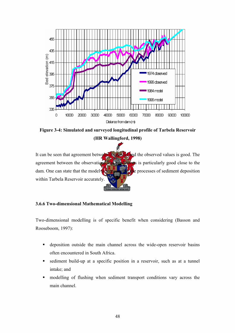
48

Figure 3-4: Simulated and surveyed longitudinal profile of Tarbela Reservoir

(HR Wallingford, 1998)

It can be seen that agreement between the model and the observed values is good. The

agreement between the observations and predictions is particularly good close to the

dam. One can state that the model is representing the processes of sediment deposition

within Tarbela Reservoir accurately.

3.6.6 Two-dimensional Mathematical Modelling

Two-dimensional modelling is of specific benefit when considering (Basson and

Rooseboom, 1997):

deposition outside the main channel across the wide-open reservoir basins

often encountered in South Africa.

sediment build-up at a specific position in a reservoir, such as at a tunnel

intake; and

modelling of flushing when sediment transport conditions vary across the

main channel.

49

3.6.7 The Quasi-2D Stream Tube Concept

A simple approach to two-dimensional modelling may be used for reservoirs. In this

the reservoir is assumed to be sub-divided into a series of stream-tubes (Batuca and

Jordaan, 2000).

Lopez (1978) most probably developed the first quasi two-dimensional models for

reservoir sedimentation, based on the stream tube concept of Holly and Cunge (1975).

The river-reservoir system was divided for modeling purposes into three distinct

zones: a) the river zone, upstream of the reservoir, where one-dimensional unsteady

flow and sediment transport were assumed, b) the transition zone from the river to the

reservoir, where the flow was simulated by means of jet theory, and c) the reservoir

zone, where the flow and sediment transport were simulated by means of the stream-

tube concept in order to obtain the longitudinal and transverse distribution of sediment

within the reservoir.

The discharge through each stream-tube is assumed to be constant. The initial

conditions are established for the starting (upstream) section. The cross-sectional

areas are not constant, but vary in such a way as to maintain constant discharge in

each stream-tube. The dispersion process is broken down into:

a) the streamwise advection in each tube:

[ ] 0CA AuCt x

∂ ∂+ =

∂ ∂ (3-59)

b) the streamwise diffusion in each tube:

xxC CA ADt x x

∂ ∂ ∂⎡ ⎤= ⎢ ⎥∂ ∂ ∂⎣ ⎦ (3-60)

c) and the transverse diffusion between neighbouring stream-tubes:

Txy Txyavg avg

C C CA y D y Dt y y

⎡ ⎤ ⎡ ⎤∂ ∂ ∂= ⋅ − ⋅⎢ ⎥ ⎢ ⎥∂ ∂ ∂⎣ ⎦ ⎣ ⎦

(3-61)

50

where y is the depth of the flow and TxyD is the coefficient of turbulence in the

transverse direction. The terms within brackets in the above equation represent the

mean conditions within a stream-tube.

It is assumed that the transverse velocities are small compared to the streamwise

velocities. Holly and Cunge (1975) used the following equations for the turbulence

coefficients: 5.93TxxD u y= ⋅ ⋅ and 0.23TyyD u y= ⋅ ⋅ . These approximations are

sufficient for river and reservoir applications, but for coastal and estuarial problems

the turbulent flow field is often more complex than this.

Generally 2D modelling is either depth-integrated or width-integrated. The depth-

integrated model is more often used in river and reservoir engineering analysis. This

model applies to simulating shallow water flow and is governed by the depth-

integrated continuity and Navier-Stokes equations (Wang and Wu, 2004):

( ) ( ) 0h hU hV

t x y∂ ∂ ∂

+ + =∂ ∂ ∂

(3-62)

( )( )( ) ( ) ( ) 1 1

1 ( )

xy xys xx xx

sx bx c

hT Dz hT DhU hUU hVU ght x y x x y x y

f hV

ρ ρ

τ τρ

∂ ∂∂ ∂ ∂∂ ∂ ∂+ + = − + + + +

∂ ∂ ∂ ∂ ∂ ∂ ∂ ∂

+ − +

(3-63)

( ) ( )( ) ( ) ( ) 1 1

1 ( )

yx yy yx yys

sy by c

hT hT D DzhV hUV hVV ght x y y x y x y

f hU

ρ ρ

τ τρ

∂ ∂ ∂ ∂∂∂ ∂ ∂+ + = − + + + +

∂ ∂ ∂ ∂ ∂ ∂ ∂ ∂

+ − +

(3-64)

where:

x, y= Horizontal Cartesian coordinates h= Flow depth U,V= Depth averaged flow velocities in the x- and y- directions zs= Water surface elevation g= Gravitational acceleration ρ = Density of fluid

51

cf = Coriolis coefficient

bxτ , byτ = Bed shear stresses in the x- and y- directions

sxτ , syτ = Shear stresses on the water surface caused by wind Txx, Txy, Tyx, Tyy= Depth-averaged turbulent stresses Dxx, Dxy, Dyx, Dyy= Dispersion terms due to the effect of secondary flow The depth-averaged 2D transport equation for suspended sediment is (Wang and Wu,

2004):

*

( ) ( ) ( )

( ) ( =1,2,..., )

yk k k k k xs s

sk k k

ShC UhC VhC C C Sh ht x y x x y y x y

w C C k N

ε ε

α

∂⎛ ⎞∂ ∂ ∂ ∂ ∂ ∂∂ ∂⎛ ⎞+ + = + + +⎜ ⎟⎜ ⎟∂ ∂ ∂ ∂ ∂∂ ∂ ∂ ∂ ∂⎝ ⎠ ⎝ ⎠

+ − (3-65)

where:

kC = Depth-averaged suspended load concentration

*kC = Suspended load transport capacity

sε = Turbulence diffusivity coefficient of sediment determined by /s t cvε σ= in which cσ is the turbulent Prandtl-Schmidt number, usually in the order of 0.5 to 1.0.

α = Non-equilibrium adaptation coefficient xS , yS = Dispersion terms to account for the effect of the non-uniform distributions of

flow velocity and sediment concentrations

The bed deformation can be calculated using the overall sediment balance equation or

the following equation:

'* *(1 ) ( ) ( ) / ( 1, 2,..., ) b

m sk k k bk b k sk

zp w C C q q L k Nt

α∂⎛ ⎞− = − + − =⎜ ⎟∂⎝ ⎠ (3-66)

The formulas for the suspended load and bed load can be written as:

*

*k bk kC p C= **b k bk bkq p q= ( 1, 2,..., )k N= (3-67)

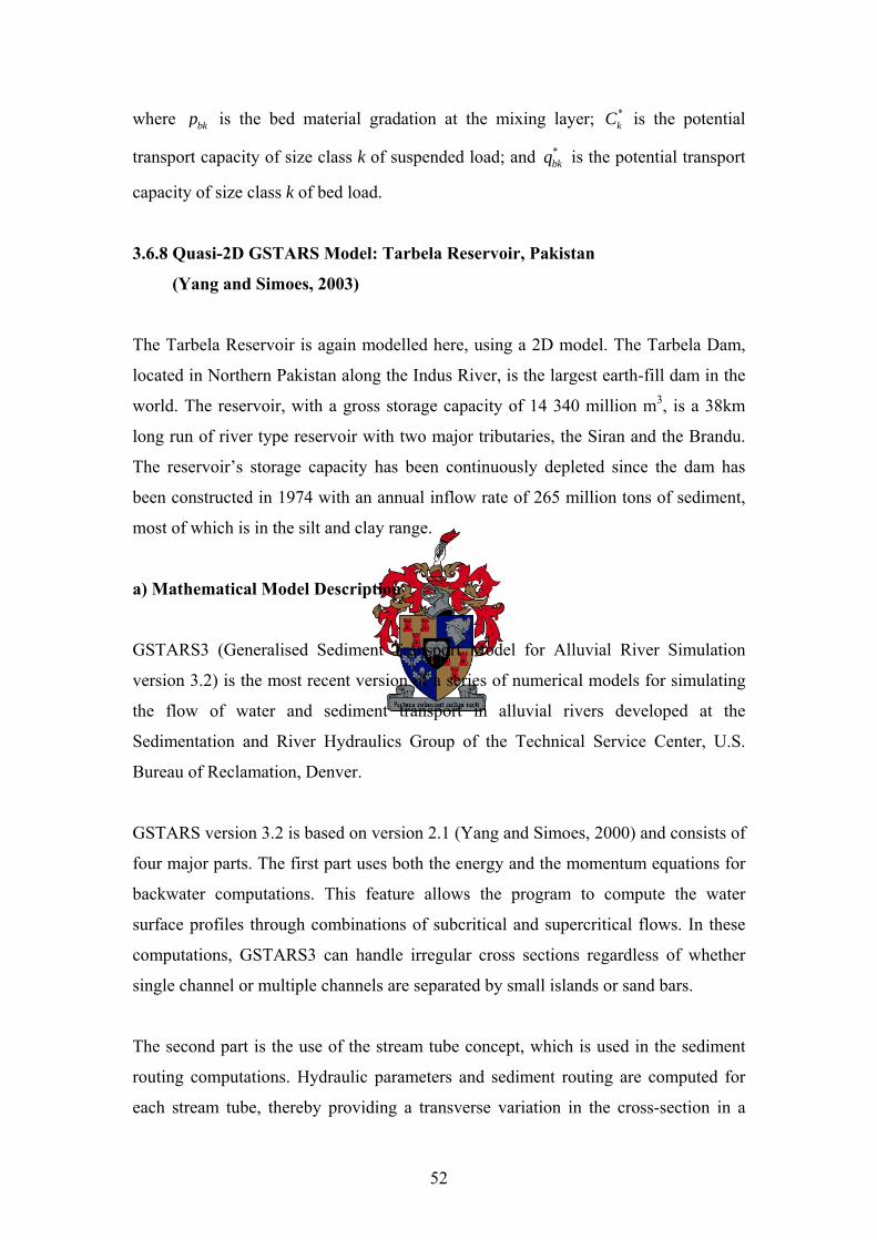
52

where bkp is the bed material gradation at the mixing layer; *kC is the potential

transport capacity of size class k of suspended load; and *bkq is the potential transport

capacity of size class k of bed load.

3.6.8 Quasi-2D GSTARS Model: Tarbela Reservoir, Pakistan

(Yang and Simoes, 2003)

The Tarbela Reservoir is again modelled here, using a 2D model. The Tarbela Dam,

located in Northern Pakistan along the Indus River, is the largest earth-fill dam in the

world. The reservoir, with a gross storage capacity of 14 340 million m3, is a 38km

long run of river type reservoir with two major tributaries, the Siran and the Brandu.

The reservoir’s storage capacity has been continuously depleted since the dam has

been constructed in 1974 with an annual inflow rate of 265 million tons of sediment,

most of which is in the silt and clay range.

a) Mathematical Model Description

GSTARS3 (Generalised Sediment Transport Model for Alluvial River Simulation

version 3.2) is the most recent version of a series of numerical models for simulating

the flow of water and sediment transport in alluvial rivers developed at the

Sedimentation and River Hydraulics Group of the Technical Service Center, U.S.

Bureau of Reclamation, Denver.

GSTARS version 3.2 is based on version 2.1 (Yang and Simoes, 2000) and consists of

four major parts. The first part uses both the energy and the momentum equations for

backwater computations. This feature allows the program to compute the water

surface profiles through combinations of subcritical and supercritical flows. In these

computations, GSTARS3 can handle irregular cross sections regardless of whether

single channel or multiple channels are separated by small islands or sand bars.

The second part is the use of the stream tube concept, which is used in the sediment

routing computations. Hydraulic parameters and sediment routing are computed for

each stream tube, thereby providing a transverse variation in the cross-section in a

53

semi two-dimensional manner. Although no flow should be transported across the

boundary of a stream tube, transverse bed slopes and secondary flows are phenomena

accounted for in GSTARS3 that contribute to the exchange of sediments between

stream tubes. The position and width of each stream tube may change after each step

of computation. The scour or deposition computed in each stream tube gives the

variation of channel geometry in the vertical (or lateral) direction. The water surface

profiles are computed first. The channel is then divided into a selected number of

stream tubes with the following characteristics: (1) the total discharge carried by the

channel is distributed equally among the stream tubes; (2) stream tubes are bounded

by channel boundaries and by imaginary walls; (3) the discharge along each stream

tube is constant (i.e., there is no exchange of water through stream tube boundaries).

The third part is the use of the theory of minimum energy dissipation rate (Yang,

1976; Yang and Song, 1986) in it’s simplified version of minimum total stream power

to compute channel width and depth adjustments. The use of this theory allows the

channel to be treated as an unknown variable, which is one of the most important

capabilities of GSTARS3. Whether a channel width or depth is adjusted at a given

time step depends on which condition results in less total stream power.

The fourth part is the inclusion of a channel bank side stability criteria based on the

angle of repose of bank materials and sediment continuity. GSTARS is a general

mathematical model developed for a personal computer to simulate and predict river

and reservoir morphological changes caused by natural and engineering events.

Although GSTARS3 is intended to be used as a general engineering tool for solving

fluvial hydraulic problems, it does have the following limitations from a theoretical

point of view (Yang and Simoes, 2003):

a) GSTARS3 is a quasi-steady flow model. Water discharge hydrographs are

approximated by bursts of constant discharges. Consequently , GSTARS3 should

not be applied to rapid, varied, unsteady flow conditions.

b) GSTARS3 is a semi-two-dimensional model for flow simulation and a semi-three-

dimensional model for simulation of channel geometry change. It should not be

54

applied to situations where a truly two-dimensional or truly three-dimensional

model is needed for detailed simulation of local conditions.

c) GSTARS3 is based on the stream tube concept. Secondary currents are

empirically accounted for. The phenomena of diffusion and super elevation are

ignored.

d) Many of the methods and concepts used in GSTARS3 are simplified

approximations of real phenomena. Those approximations and their limits of

validity are therefore embedded in the model.

b) Model Setup

In this example, GSTARS3 is used to simulate 22 years of reservoir sedimentation

(from 1974 through 1996) for a reach that spans nearly 95 kilometres upstream from

the Tarbela Dam (see Figure 3-5). The hydrology of the system is depicted in Figure

3-6, together with dam operation information. The tributaries make a relatively small

contribution when compared to the main stem discharge, therefore they are not

included in Figure 3-6 (they are however included in the computations).

There is a percentage of silt and clay in the sediments being transported, but there is

no data to simulate them using the Krone/Ariathurai methods. Secondly, analysis of

the 1996 cross-sectional data suggests that deposition occurs in the form of a

horizontal fill as can be observed in Figure 3-7.

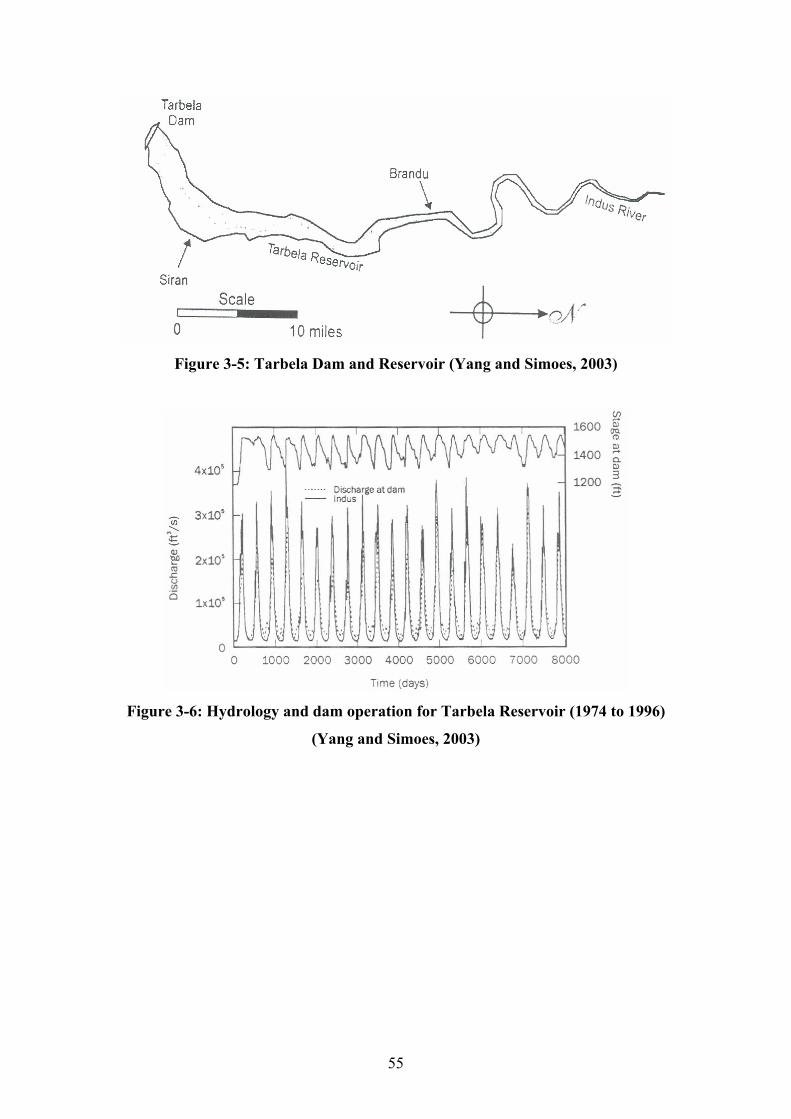
55

Figure 3-5: Tarbela Dam and Reservoir (Yang and Simoes, 2003)

Figure 3-6: Hydrology and dam operation for Tarbela Reservoir (1974 to 1996)

(Yang and Simoes, 2003)

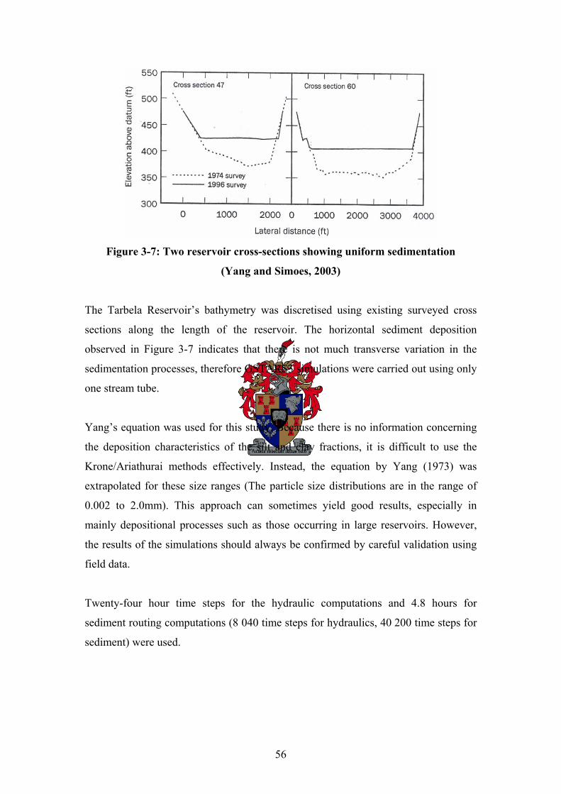
56

Figure 3-7: Two reservoir cross-sections showing uniform sedimentation

(Yang and Simoes, 2003)

The Tarbela Reservoir’s bathymetry was discretised using existing surveyed cross

sections along the length of the reservoir. The horizontal sediment deposition

observed in Figure 3-7 indicates that there is not much transverse variation in the

sedimentation processes, therefore GSTARS3 simulations were carried out using only

one stream tube.

Yang’s equation was used for this study. Because there is no information concerning

the deposition characteristics of the silt and clay fractions, it is difficult to use the

Krone/Ariathurai methods effectively. Instead, the equation by Yang (1973) was

extrapolated for these size ranges (The particle size distributions are in the range of

0.002 to 2.0mm). This approach can sometimes yield good results, especially in

mainly depositional processes such as those occurring in large reservoirs. However,

the results of the simulations should always be confirmed by careful validation using

field data.

Twenty-four hour time steps for the hydraulic computations and 4.8 hours for

sediment routing computations (8 040 time steps for hydraulics, 40 200 time steps for

sediment) were used.

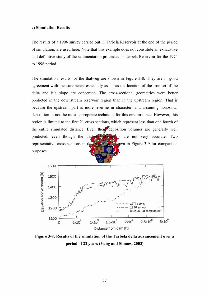
57

c) Simulation Results

The results of a 1996 survey carried out in Tarbela Reservoir at the end of the period

of simulation, are used here. Note that this example does not constitute an exhaustive

and definitive study of the sedimentation processes in Tarbela Reservoir for the 1974

to 1996 period.

The simulation results for the thalweg are shown in Figure 3-8. They are in good

agreement with measurements, especially as far as the location of the frontset of the

delta and it’s slope are concerned. The cross-sectional geometries were better

predicted in the downstream reservoir region than in the upstream region. That is

because the upstream part is more riverine in character, and assuming horizontal

deposition in not the most appropriate technique for this circumstance. However, this

region is limited to the first 21 cross sections, which represent less than one fourth of

the entire simulated distance. Even then, deposition volumes are generally well

predicted, even though the thalweg elevations are not very accurate. Two

representative cross-sections in this region are shown in Figure 3-9 for comparison

purposes.

Figure 3-8: Results of the simulation of the Tarbela delta advancement over a

period of 22 years (Yang and Simoes, 2003)

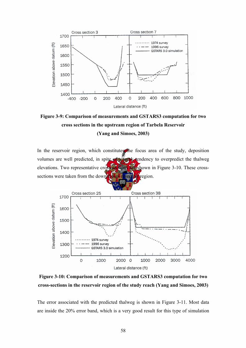
58

Figure 3-9: Comparison of measurements and GSTARS3 computation for two

cross sections in the upstream region of Tarbela Reservoir

(Yang and Simoes, 2003)

In the reservoir region, which constitutes the focus area of the study, deposition

volumes are well predicted, in spite of a weak tendency to overpredict the thalweg

elevations. Two representative cross sections are shown in Figure 3-10. These cross-

sections were taken from the downstream reservoir region.

Figure 3-10: Comparison of measurements and GSTARS3 computation for two

cross-sections in the reservoir region of the study reach (Yang and Simoes, 2003)

The error associated with the predicted thalweg is shown in Figure 3-11. Most data

are inside the 20% error band, which is a very good result for this type of simulation

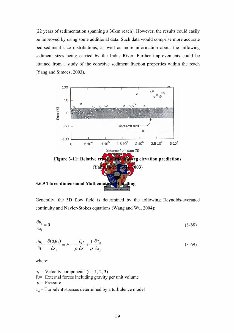
59

(22 years of sedimentation spanning a 36km reach). However, the results could easily

be improved by using some additional data. Such data would comprise more accurate

bed-sediment size distributions, as well as more information about the inflowing

sediment sizes being carried by the Indus River. Further improvements could be

attained from a study of the cohesive sediment fraction properties within the reach

(Yang and Simoes, 2003).

Figure 3-11: Relative error of the thalweg elevation predictions

(Yang and Simoes, 2003)

3.6.9 Three-dimensional Mathematical Modelling

Generally, the 3D flow field is determined by the following Reynolds-averaged

continuity and Navier-Stokes equations (Wang and Wu, 2004):

0i

i

ux∂

=∂

(3-68)

( ) 1 1i j iji i

ij i j

u uu pFt x x x

τρ ρ

∂ ∂∂ ∂+ = − +

∂ ∂ ∂ ∂ (3-69)

where: ui-= Velocity components (i = 1, 2, 3) Fi= External forces including gravity per unit volume p = Pressure

ijτ = Turbulent stresses determined by a turbulence model

60

For shallow water flow, the pressure variation can be assumed to be hydrostatic and

all the vertical components of fluid acceleration can be ignored, thus yielding the

quasi-3D governing equation (Wang and Wu, 2004):

0u v wx y z∂ ∂ ∂

+ + =∂ ∂ ∂

(3-70)

( ) ( ) ( ) 1 1 1xys xx xzzu uu vu wu g fv

t x y z x x y zττ τ

ρ ρ ρ∂∂ ∂ ∂∂ ∂ ∂ ∂

+ + + = − + + + +∂ ∂ ∂ ∂ ∂ ∂ ∂ ∂

(3-71)

( ) ( ) ( ) 1 1 1yx yy yzszv uv vv wv g fu

t x y z y x y zτ τ τ

ρ ρ ρ∂ ∂ ∂∂∂ ∂ ∂ ∂

+ + + = − + + + −∂ ∂ ∂ ∂ ∂ ∂ ∂ ∂

(3-72)

where f is the Coriolis coefficient. The hydrostatic pressure variation assumption brings significant simplification to the

full 3D equations 3-68 and 3-69. However, this simplification is valid only for

gradually varying open-channel flows. A full 3D model without this simplification

should be used in regions of rapidly varying flows.

Sediment transport is sub-divided into a suspended load and a bed load and hence the

flow domain is divided into a bed-load layer with thickness δ and the suspended load

layer above it with thickness h -δ . The exchange of sediment between the two layers

is through deposition (downward sediment flux) at a rate of bkD and the entrainment

from the bed load layer (upward flux) at a rate of bkE . The distribution of the sediment

concentration in the upper layer is governed by the following advection-dispersion

equation:

3[( ) ]j sk j kk t k

j j c j

u w cc v ct x x x

δσ⎛ ⎞∂ −∂ ∂∂

+ = ⎜ ⎟⎜ ⎟∂ ∂ ∂ ∂⎝ ⎠ (3-73)

where kc is the local concentration of the k-th size class of suspended sediment load;

3jδ is the Kronecker delta with j=3 indicating the vertical direction. At the free

surface, the vertical sediment flux is zero and hence the condition applied is:

61

0t ksk k

c

v c w czσ

∂+ =

∂ (3-74)

At the lower boundary of the suspended sediment layer, the deposition rate is

bk sk bkD w c= , while the entrainment rate, bkE equals:

*t k

bk sk b kc

v cE w czσ

∂= − =

∂ (3-75)

where *b kc is the equilibrium concentration at the reference level bz z δ= + , which

needs to be determined by using an empirical relation. In the 3D model, the bed load

transport is simulated by using the equation:

*

( )( ) ( ) 1 ( ) 0 ( 1, 2,..., )by bkb bk bx bkbk b k

qc q q q k Nt x y L

αδ α ∂∂ ∂+ + + − = =

∂ ∂ ∂ (3-76)

where bkc is the average concentration of bed load in the bed load zone, bkq is the bed

load transport rate of the k-th size class and *b kq is the corresponding bed load

transport capacity. bxα and byα are the direction cosines of the bed shear stresses,

known from the flow calculation.

The bed change can be determined by either the exchange equation:

*1(1 ' ) ( )b

m bk bk bk b kk s

zp D E q qt L

∂⎛ ⎞− = − + −⎜ ⎟∂⎝ ⎠ (3-77)

or the overall sediment mass-balance equation integrated over the water depth h:

( )(1 ' ) 0tkyb tk tkxm

k

qz hC qpt t x y

∂∂ ∂ ∂⎛ ⎞− = + + =⎜ ⎟∂ ∂ ∂ ∂⎝ ⎠ (3-78)

where tkC is the depth-averaged sediment concentration and tkxq and tkyq are the

components of the total load sediment transport in the x- and y- directions:

62

; h h

t k t ktkx bx bk k tky by bk k

c c

v c v cq q uc z q q vc zx xδ δ

α ασ σ

⎛ ⎞ ⎛ ⎞∂ ∂= + − ∂ = + − ∂⎜ ⎟ ⎜ ⎟∂ ∂⎝ ⎠ ⎝ ⎠

∫ ∫ (3-79)

3.6.10 Three-dimensional Model: Three Gorges Reservoir Project, China (Dou et al., 2004) This study applies a 3D mathematical model for suspended load motion in turbulent

flows and is based on the following new components:

• A new stress model based on the stochastic theory of turbulent flows by

Dou (1980)

• Refined wall function for treatment of solid walls

• Introduction of traditional equations of suspended load motion and sorting

of bed material into a 3D model

• Orthogonal curvilinear grid system, with horizontal layers employed over

the water depth

The equation system is solved by using the SIMPLE–C algorithmic. The above model is

first validated using hydrological data collected before and after the construction of the

existing Gezhouba Dam. The model is then applied to the sedimentation problem of the

much larger Three Gorges Project (located upstream of the Gezhouba Dam) and

predictions are made of the sediment deposition pattern, the size distribution of the

deposits and the flow fields.

a) Background

The dam area of the Three Gorges Project is located within Xiling Gorge on the

Yangtze River. A 16km long river reach was simulated between Miaohe and the dam

axis at Sandouping, a deep valley of heavily weathered anticline diorite and granite,

with low mountains and hills on both sides. The width of the river in this section is

usually 600m to 700m during a flooding period. The maximum width of 1 400m is

found near Sandouping. The river reach under investigation contains slight bends. The

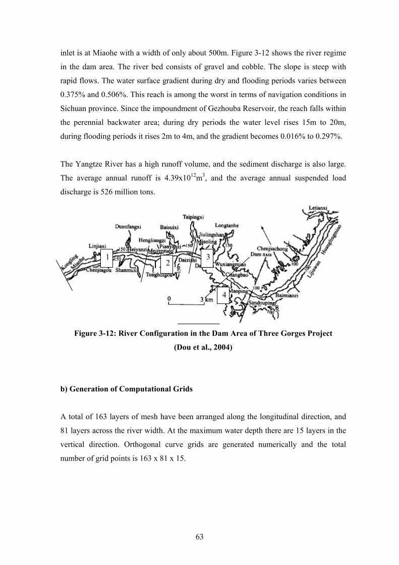
63

inlet is at Miaohe with a width of only about 500m. Figure 3-12 shows the river regime

in the dam area. The river bed consists of gravel and cobble. The slope is steep with

rapid flows. The water surface gradient during dry and flooding periods varies between

0.375% and 0.506%. This reach is among the worst in terms of navigation conditions in

Sichuan province. Since the impoundment of Gezhouba Reservoir, the reach falls within

the perennial backwater area; during dry periods the water level rises 15m to 20m,

during flooding periods it rises 2m to 4m, and the gradient becomes 0.016% to 0.297%.

The Yangtze River has a high runoff volume, and the sediment discharge is also large.

The average annual runoff is 4.39x1012m3, and the average annual suspended load

discharge is 526 million tons.

Figure 3-12: River Configuration in the Dam Area of Three Gorges Project

(Dou et al., 2004)

b) Generation of Computational Grids A total of 163 layers of mesh have been arranged along the longitudinal direction, and

81 layers across the river width. At the maximum water depth there are 15 layers in the

vertical direction. Orthogonal curve grids are generated numerically and the total

number of grid points is 163 x 81 x 15.

1 2

3

4

64

c) Verification of Deposition in the Three Gorges Dam Site Area Due to Gezhouba

Reservoir

A period of three years was selected for the reservoir sedimentation verification (from

June 1981, after the impoundment of the existing Gezhouba Reservoir to December

1984) Calculation time steps were 3 to 4 days on average. Calculation of sediment

concentration of suspended load was performed for 7 grain size groups, and the average

values during the period 1981 to 1984 were used for the percentage of each grain size.

Table 3-1 provides a comparison between calculated and measured amounts of

deposition for the reaches numbered 1 to 4 on Figure 3-12. It can be seen from Table 3

that the predictions were quite close to the measured values.

Table 3-1: Comparison between the calculated and measured deposits for different

reaches (104 m3) (Dou et al., 2004)

Reach 1 2 3 4 Total Calculated 271.2 231.9 300.4 432.6 1236.1 Measured 310.5 224.6 240.4 418 1193.5 Error (%) -12.7 3.2 25 3.5 3.6

d) Calculation Conditions for Predictions of the Three Gorges Project

The incoming hydrographs of runoff and graded suspended load entering Three Gorges

Project dam area have been provided by the Yangtze River Scientific Research Institute

based on a 1D model.

During initial operation of the reservoir both the amount of suspended load and the grain

sizes will be small. After 90 year of operation, most suspended load will reach the dam

area and the median diameter will be increased to 0.027mm, close to the average annual

median diameter of natural suspended load, i.e. 0.031mm, For large discharges, the

median diameter could be larger than 0.031mm.

Though the grain size distribution of suspended sediment entering the dam area may

vary with time and discharge, it is assumed that the size distribution is related to D50.

65

In this model study, the following equation by Zhou (1997) was used. It is based on

statistical analysis of data from the Yangtze River Scientific Research Institute:

500.639

1LD

dLP e

⎛ ⎞− ⎜ ⎟

⎝ ⎠= − (3-80)

where DL is the representative grain size (mm), PL the percentage by weight of the

sediment interval in question. The above equation is used for determining the size

distribution of suspended load. A total of 7 intervals for suspended load were used in the

calculation.

e) Hydrological Series in the Simulation

The hydrological series adopted for the calculation is a 10-year series, based on

observed data during the period 1961 to 1970. The average incoming water and

sediment loads during the 10 years is close to the annual averaged amounts, and are

considered to be representative. In order to take into consideration the impact of extra-

large flood and sediment years during long-term simulation, it has been suggested that

after 30 years of operation of the reservoir an extra high- flood-high-sediment year,

1954, be inserted into the hydrological series. In total, a period of 76 years was

simulated.

f) Sediment Deposition at the Upper Reach of the Dam Area

Figure 3-13 depicts deposition development of the entire 16km reach compared to that

of the 6.8km near dam reach.

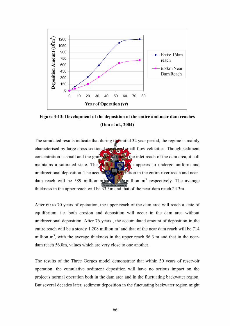
66

0

150

300

450

600

750

900

1050

1200

0 10 20 30 40 50 60 70 80

Year of Operation (yr)

Dep

ositi

on A

mou

nt (1

06 m3 )

Entire 16kmreach

6.8km NearDam Reach

Figure 3-13: Development of the deposition of the entire and near dam reaches

(Dou et al., 2004)

The simulated results indicate that during the initial 32 year period, the regime is mainly

characterised by large cross-sectional areas and small flow velocities. Though sediment

concentration is small and the grain size is fine at the inlet reach of the dam area, it still

maintains a saturated state. The entire river reach appears to undergo uniform and

unidirectional deposition. The accumulated deposition in the entire river reach and near-

dam reach will be 589 million m3 and 312 million m3 respectively. The average

thickness in the upper reach will be 33.3m and that of the near-dam reach 24.3m.

After 60 to 70 years of operation, the upper reach of the dam area will reach a state of

equilibrium, i.e. both erosion and deposition will occur in the dam area without

unidirectional deposition. After 76 years , the accumulated amount of deposition in the

entire reach will be a steady 1.208 million m3 and that of the near dam reach will be 714

million m3, with the average thickness in the upper reach 56.3 m and that in the near-

dam reach 56.0m, values which are very close to one another.

The results of the Three Gorges model demonstrate that within 30 years of reservoir

operation, the cumulative sediment deposition will have no serious impact on the

project's normal operation both in the dam area and in the fluctuating backwater region.

But several decades later, sediment deposition in the fluctuating backwater region might

67

affect the navigation and harbour operation during extremely dry years when the

reservoir's water surface drops down to it’s lowest level.

g) Sediment Concentration Field

The largest difference between 3D and 2D models is that 2D models can only simulate

depth-averaged flow fields and sediment concentration fields, while 3D models can

predict flow fields and sediment concentration fields at different water depths or

elevations. The 3D simulated results however show that the distribution of sediment

concentrations over the depth is relatively uniform. Sediment concentration at the

riverbed is slightly larger than that in the middle and near the surface.

h) Bed Material Constituents

The simulated results show that the average bed grain size after 76 years of operation

is between 0.057mm and 0.062mm.

3.7 Density Currents

Apart from turbulent suspended sediment transport, which is the dominant mechanism

by which sediment is transported through most reservoirs, density currents in certain

reservoirs provide an additional mechanism to transport sediment.

Density differences often exist between discharges in tributaries and receiving

reservoirs. These inflows tend to plunge when their densities are greater than those of

the surface layer in the receiving system, entering as density currents or turbidity

currents. If the density of the inflow is less than that of the surface layer, the inflow

will tend to travel along the surface, thus entering as an overflow. If local mixing is

inadequate in the region of the inflow to eliminate density differences, the density or

turbidity current will plunge and travel along the sloping bottom as an underflow.

These processes are accompanied by entrainment of ambient water. If a depth is

encountered where the density of the underflow equals that of the water column, the

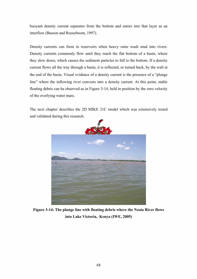
68

buoyant density current separates from the bottom and enters into that layer as an

interflow (Basson and Rooseboom, 1997).

Density currents can form in reservoirs when heavy rains wash mud into rivers.

Density currents commonly flow until they reach the flat bottom of a basin, where

they slow down, which causes the sediment particles to fall to the bottom. If a density

current flows all the way through a basin, it is reflected, or turned back, by the wall at

the end of the basin. Visual evidence of a density current is the presence of a “plunge

line” where the inflowing river converts into a density current. At this point, stable

floating debris can be observed as in Figure 3-14, held in position by the zero velocity

of the overlying water mass.

The next chapter describes the 2D MIKE 21C model which was extensively tested

and validated during this research.

Figure 3-14: The plunge line with floating debris where the Nzoia River flows

into Lake Victoria, Kenya (IWE, 2005)

69

4. THE MIKE 21C MATHEMATICAL SEDIMENTATION MODEL

4.1 Background

MIKE 21C is a 2D curvilinear modelling tool for the simulation of morphological

changes in rivers and reservoirs. It incorporates a varying size mesh design with state-

of-the-art hydrodynamic and morphological technology.

The model components can run simultaneously, thus incorporating dynamic feedback

from changing hydraulic resistance, bed topography and bank lines affecting the

hydro-dynamic behaviour of the river or reservoir (DHI, 2003).

Creating a hydrodynamic river or reservoir model using MIKE 21C involves the

following four steps:

The extent of the modeling area is selected and the computational grid is

designed for the river or reservoir area.

The bathymetry is entered onto the computational grid, i.e. bed levels are

specified in each computational grid point. This is done by creating a data

input file of coordinates and their heights above sea level. The processes used

to determine this data typically involves conversions, interpolation and

extrapolation of coordinates and their heights from survey data.

Specification of the boundary conditions for instance a time series of discharge

at the inflow boundary, and a time series of water level at the downstream

model boundary.

Either of the two simulation modules is chosen. The first option is

‘Hydrodynamics only’ which only gives the output of water depth, surface

elevation, unit discharges and velocities throughout the model. The other

option is ‘Hydrodynamics and river morphology’ which in addition gives as

output the changes in the bed levels due to sediment transport, deposition and

erosion.

70

The complete modelling procedure is described in the following section, including

grid generation, bathymetry development, choice of hydrodynamic and sediment

transport models. The order of the topics is as it is found on the MIKE 21C

Curvilinear Flow Model setup interface.

4.2 Basic Setup Parameters

4.2.1 Generation of the Curvilinear Grid

MIKE 21C is designed to function on an orthogonal curvilinear grid. The numerical

grid is created by means of the Grid Generator utility program. To do this an accurate

description of the bank lines is required within which the grid is drawn. The

coordinates of bank lines can be derived from orthophotos or survey data. The

amount of grid cells in the flow direction and also across the flow is then chosen after

which the grid is automatically generated with an anisotropic conformal mapping

method by the Grid Generator. Often the shape of the generated gridlines and cells

does not accurately describe the topography or expected flow pattern and the cells

must then be reshaped by hand.

Generation of an orthogonal curvilinear grid is an iterative process in which gridlines

are smoothened until the computational grid is acceptable and without unacceptably

large gradients in grid cell spacing and curvature of grid lines. This is the most time

consuming part of setting up any model and also the most important since it forms the

basis of a reliable simulation model. It is important to keep in mind that the size of the

grid determines the run time of the simulation since the calculations of

hydrodynamics and sediment transport are done at every single grid point at every

time-step. Therefore with more cells the output will be more detailed, but the

computational time will increase.

Initial hydrodynamic simulations may still reveal the need for further refinements and

adjustments of the grid. It is preferable to use cells that are elongated in the flow

direction for these types of models. To keep the simulation from becoming unstable,

the water should not be allowed to flow through the length of one grid cell within one

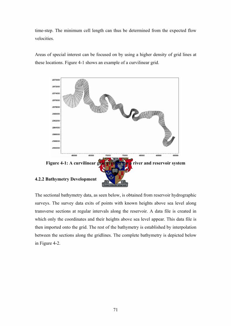
71

time-step. The minimum cell length can thus be determined from the expected flow

velocities.

Areas of special interest can be focused on by using a higher density of grid lines at

these locations. Figure 4-1 shows an example of a curvilinear grid.

Figure 4-1: A curvilinear grid created for a river and reservoir system

4.2.2 Bathymetry Development

The sectional bathymetry data, as seen below, is obtained from reservoir hydrographic

surveys. The survey data exits of points with known heights above sea level along

transverse sections at regular intervals along the reservoir. A data file is created in

which only the coordinates and their heights above sea level appear. This data file is

then imported onto the grid. The rest of the bathymetry is established by interpolation

between the sections along the gridlines. The complete bathymetry is depicted below

in Figure 4-2.

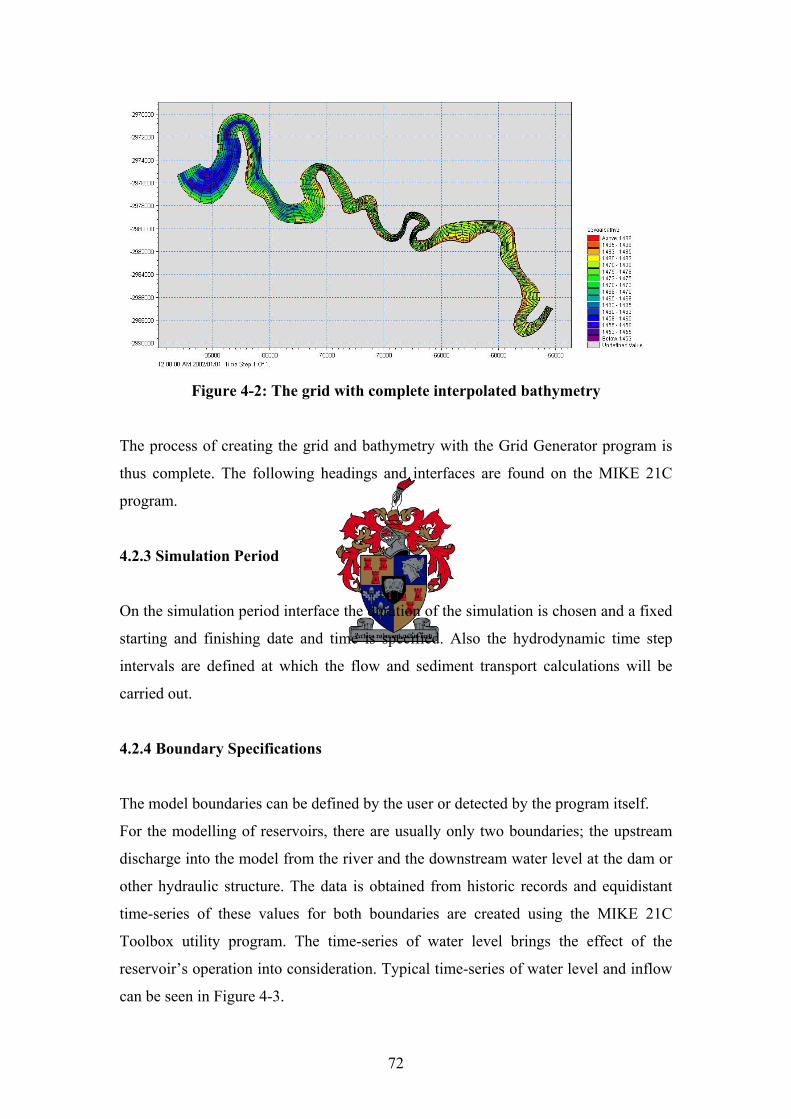
72

Figure 4-2: The grid with complete interpolated bathymetry

The process of creating the grid and bathymetry with the Grid Generator program is

thus complete. The following headings and interfaces are found on the MIKE 21C

program.

4.2.3 Simulation Period

On the simulation period interface the duration of the simulation is chosen and a fixed

starting and finishing date and time is specified. Also the hydrodynamic time step

intervals are defined at which the flow and sediment transport calculations will be

carried out.

4.2.4 Boundary Specifications

The model boundaries can be defined by the user or detected by the program itself.

For the modelling of reservoirs, there are usually only two boundaries; the upstream

discharge into the model from the river and the downstream water level at the dam or

other hydraulic structure. The data is obtained from historic records and equidistant

time-series of these values for both boundaries are created using the MIKE 21C

Toolbox utility program. The time-series of water level brings the effect of the

reservoir’s operation into consideration. Typical time-series of water level and inflow

can be seen in Figure 4-3.

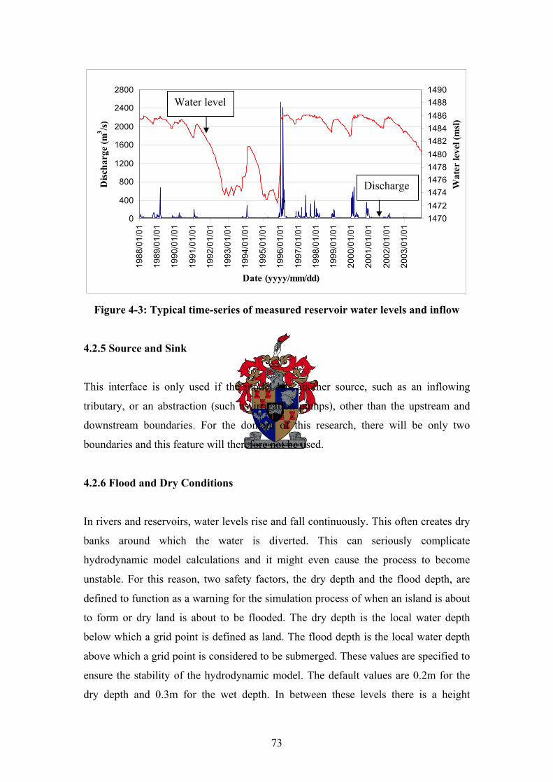
73

0

400

800

1200

1600

2000

2400

2800

1988

/01/

01

1989

/01/

01

1990

/01/

01

1991

/01/

01

1992

/01/

01

1993

/01/

01

1994

/01/

01

1995

/01/

01

1996

/01/

01

1997

/01/

01

1998

/01/

01

1999

/01/

01

2000

/01/

01

2001

/01/

01

2002

/01/

01

2003

/01/

01

Date (yyyy/mm/dd)

Disc

harg

e (m

3 /s)

14701472147414761478148014821484148614881490

Wat

er le

vel (

msl)

Figure 4-3: Typical time-series of measured reservoir water levels and inflow

4.2.5 Source and Sink

This interface is only used if the model has another source, such as an inflowing

tributary, or an abstraction (such as irrigation pumps), other than the upstream and

downstream boundaries. For the domain of this research, there will be only two

boundaries and this feature will therefore not be used.

4.2.6 Flood and Dry Conditions

In rivers and reservoirs, water levels rise and fall continuously. This often creates dry

banks around which the water is diverted. This can seriously complicate

hydrodynamic model calculations and it might even cause the process to become

unstable. For this reason, two safety factors, the dry depth and the flood depth, are

defined to function as a warning for the simulation process of when an island is about

to form or dry land is about to be flooded. The dry depth is the local water depth

below which a grid point is defined as land. The flood depth is the local water depth

above which a grid point is considered to be submerged. These values are specified to

ensure the stability of the hydrodynamic model. The default values are 0.2m for the

dry depth and 0.3m for the wet depth. In between these levels there is a height

Water level

Discharge

74

difference to avoid alternative swapping, which can lead to instability of the

hydrodynamic calculations (DHI, 2003).

For the reservoir models described in this research, the entire model domain will

remain wet. These models are not expected to experience wetting and drying, but

because of changing bed levels due to sedimentation, it can occur. The default values

are used throughout this research.

4.3 Hydrodynamic Parameters

4.3.1 Initial Surface Elevation

This is the initial surface level at the start of the simulation. This can either be a

constant horizontal level throughout the whole model domain or it can have an initial

hydraulic gradient as defined by an input data file. All the reservoirs that were

modelled in this research had an initial hydraulic gradient merely to initiate flow in

the right direction. Some model simulations, mostly those with low discharges and

water levels, even became unstable when this technique was not implemented.

4.3.2 Eddy Viscosity

The eddy viscosity is taken as constant throughout the model. If the model is applied

to a reservoir system, this value can be taken as 0.01m2/s. For small scale models such

as flumes with small grid spacing relative to the depth, the eddy viscosity may be

neglected. Eddy viscosity becomes important when the horizontal grid spacing of a

model is much larger than the water depth, as in the case of reservoir models (DHI,

2003).

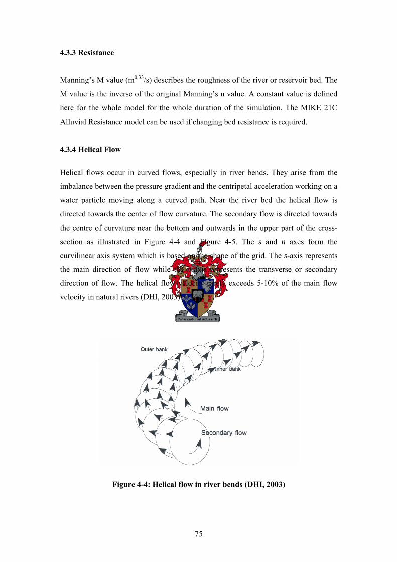
75

4.3.3 Resistance

Manning’s M value (m0.33/s) describes the roughness of the river or reservoir bed. The

M value is the inverse of the original Manning’s n value. A constant value is defined

here for the whole model for the whole duration of the simulation. The MIKE 21C

Alluvial Resistance model can be used if changing bed resistance is required.

4.3.4 Helical Flow

Helical flows occur in curved flows, especially in river bends. They arise from the

imbalance between the pressure gradient and the centripetal acceleration working on a

water particle moving along a curved path. Near the river bed the helical flow is

directed towards the center of flow curvature. The secondary flow is directed towards

the centre of curvature near the bottom and outwards in the upper part of the cross-

section as illustrated in Figure 4-4 and Figure 4-5. The s and n axes form the

curvilinear axis system which is based on the shape of the grid. The s-axis represents

the main direction of flow while the n-axis represents the transverse or secondary

direction of flow. The helical flow velocity rarely exceeds 5-10% of the main flow

velocity in natural rivers (DHI, 2003).

Figure 4-4: Helical flow in river bends (DHI, 2003)

76

Figure 4-5: The vertical distributions of primary flow and helical flow (DHI, 2003)

The magnitude of the secondary flow can be shown to be proportional to the main

flow velocity, the depth of flow and the curvature of the main flow stream lines. The

intensity of the helical flow is the magnitude of the transverse velocity component (n-

axis) and is defined by de Vriend (1981) as:

ss

hi uR

= (4-1)

where:

u = Main flow velocity sR = Radius of curvature of streamlines

si = Helical flow intensity h = Water depth

The strength of the helical flow is used when determining the direction of both bed

and suspended load sediment transport. Secondary flow due to curving streamlines

causes a small deviation δs in the flow direction near the bed, away from the main

stream direction. This also causes a deviation in the bed shear stress direction. The

angle between bed shear stress and depth averaged shear stress (in the main flow

direction) is given by the logarithmic model by Rozovskii (1957):

77

tan ss

hR

δ β= − (4-2)

The parameter β is defined as:

2 1gC

β ακ κ2

⎛ ⎞= −⎜ ⎟⎜ ⎟

⎝ ⎠ (4-3)

where:

κ = Von Karman’s constant (0.4) g = Acceleration due to gravity (9.81 m/s2) C = Chezy friction factor α = Calibration constant

Helical flow is a principal secondary flow phenomenon in rivers and has a significant

influence on the sediment transport direction and hence the morphological changes in

the river channel. Helical flow is therefore analyzed in sediment transport simulations

when larger scale morphology is modeled. More detail about the sediment transport

and morphology models will be given in subsequent paragraphs.

Helical flow is included via the calibration constant α. This is entered either as a

constant value throughout the model domain, or as a spatially varying value from a

data file. The default value is 1.0. A limiting angle (tan δs), between the depth

averaged flow shear stress direction and the helical flow shear stress direction must

also be specified (DHI, 2003).

4.4 Hydrodynamic Integration

The hydrodynamic module simulates the water level and flow variation throughout

the model. On this menu the type of hydrodynamic integration module is chosen. It

can be either one of the following:

Fully Dynamic

Scaled Dynamic

78

Quasi-Steady

Steady

The hydrodynamics of rivers and reservoirs are characterised by complex three

dimensional flow patterns. This has to be taken into account when these systems are

modelled. However to apply a fully three dimensional model for long term

simulations of river morphology requires excessive computational efforts. By

introducing simplifications to the Navier-Stokes equations, the governing

hydrodynamic equations can be reduced to two-dimensional equations representing

conservation of momentum and mass in the two horizontal directions of a curvilinear

coordinate system (DHI, 2003).

The curvilinear coordinate system is based on the shape of the grid with the s-axis in

the main direction of flow while the n-axis represents the transverse direction of flow.

Three dimensional effects are maintained in the depth-averaged model by introducing

a separate model of the helical flow (secondary flow) component and by assuming

similarity of the vertical distribution of the main flow velocities at all computational

points. Three main approximations are adopted (DHI, 2003):

Shallow water approximation where lateral exchange of momentum due to

friction in the fluid is neglected.

In the hydrostatic pressure distribution the component of vertical velocity is

neglected

The Rigid lid approximation implies that the water surface is considered as

being a rigid impermeable and shear stress free plate.

To summarise, the flow model is valid for shallow, gently varying topography and

mild curved and wide channels with small Froude numbers. The following effects are

included in the equations when used for river and reservoir applications (DHI, 2003):

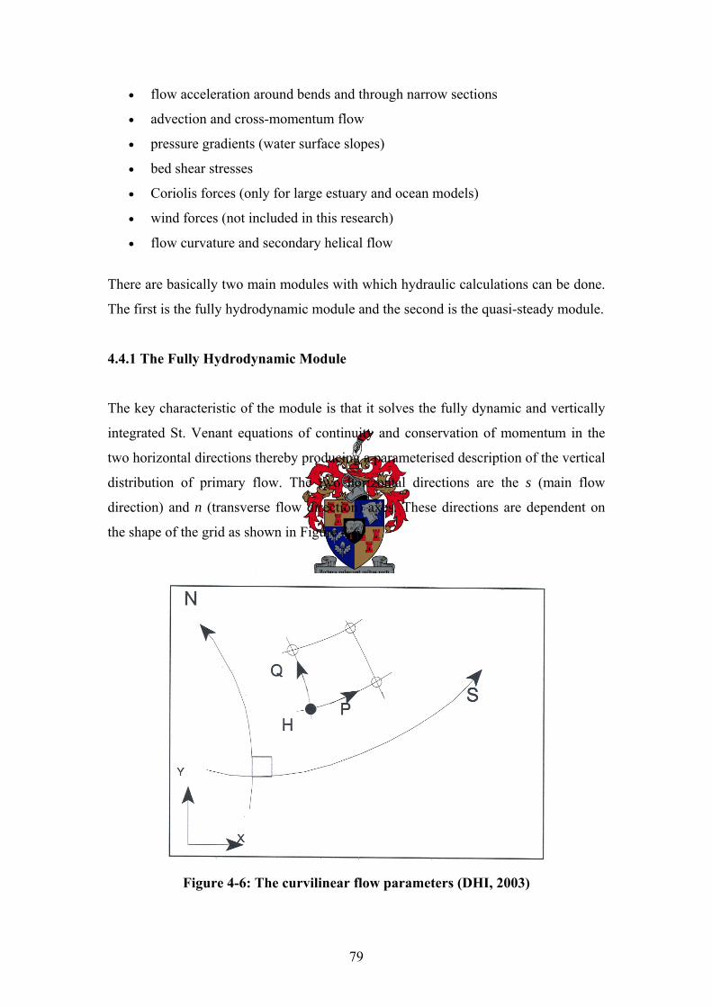
79

• flow acceleration around bends and through narrow sections

• advection and cross-momentum flow

• pressure gradients (water surface slopes)

• bed shear stresses

• Coriolis forces (only for large estuary and ocean models)

• wind forces (not included in this research)

• flow curvature and secondary helical flow

There are basically two main modules with which hydraulic calculations can be done.

The first is the fully hydrodynamic module and the second is the quasi-steady module.

4.4.1 The Fully Hydrodynamic Module

The key characteristic of the module is that it solves the fully dynamic and vertically

integrated St. Venant equations of continuity and conservation of momentum in the

two horizontal directions thereby producing a parameterised description of the vertical

distribution of primary flow. The two horizontal directions are the s (main flow

direction) and n (transverse flow direction) axes. These directions are dependent on

the shape of the grid as shown in Figure 4-6.

Figure 4-6: The curvilinear flow parameters (DHI, 2003)

80

The two horizontal axes (s and n) are described in a curvilinear orthogonal coordinate

system, where one axis follows the bank lines of the river or reservoir. This makes the

mathematical and numerical description substantially simpler. Q and P are the mass

fluxes in the s and n directions respectively, while H is the flow depth at the specific

grid point under consideration.

The curvature of the grid lines gives rise to additional terms in the partial differential

equations for the flow. The dynamic equations solved are (DHI, 2003):

2 22 2 2

2 22n s

p p qp p pq pq p q H ggh RHSt s h n h hR hR s C h

⎛ ⎞ +∂ ∂ ∂ − ∂⎛ ⎞+ + − + + + =⎜ ⎟ ⎜ ⎟∂ ∂ ∂ ∂⎝ ⎠⎝ ⎠ (4-4)

2 22 2 2

2 22s n

q p qq pq q pq q p H ggh RHSt s h n h hR hR n C h

⎛ ⎞ +∂ ∂ ∂ − ∂⎛ ⎞+ + − + + + =⎜ ⎟⎜ ⎟∂ ∂ ∂ ∂⎝ ⎠ ⎝ ⎠ (4-5)

with: 0s n

H p q q pt s n R R

∂ ∂ ∂+ + − + =

∂ ∂ ∂ (4-6)

where:

s , n = Coordinates in the curvilinear coordinate system p , q = Mass fluxes in the s- and n-directions respectively H = Water level h = Water depth g = Gravitational acceleration C = Chezy roughness coefficient

sR , nR = Radius of curvature of s- and n-line, respectively RHS = The right hand side describing a.o. Reynold stresses, Coriolis force, wind friction and atmospheric pressure

These equations can also be written in terms of the cartesian rectangular co-ordinate

system (DHI, 2003):

( ) ( )2 2 2

2 2

/ / ( / )

( / )

p h pq h gp p qp s p hgh h Et x y C h x x x

p hh Ey y

∂ ∂ +∂ ∂ ∂ ∂⎛ ⎞+ + + + = ⎜ ⎟∂ ∂ ∂ ∂ ∂ ∂⎝ ⎠⎛ ⎞∂ ∂

+ ⎜ ⎟∂ ∂⎝ ⎠

(4-7)

81

( ) ( )2 2 2

2 2

// ( / )

( / )

q hpq h gp p qq s q hgh h Et x y C h y x x

q hh Ey y

∂∂ +∂ ∂ ∂ ∂⎛ ⎞+ + + + = ⎜ ⎟∂ ∂ ∂ ∂ ∂ ∂⎝ ⎠⎛ ⎞∂ ∂

+ ⎜ ⎟∂ ∂⎝ ⎠

(4-8)

where: 0h p qt x y

∂ ∂ ∂+ + =

∂ ∂ ∂ (4-9)

and E is the eddy viscosity.

4.4.2 The Quasi-steady Hydrodynamic Module

This solver is a predictor-corrector algorithm that originates from methods for

incompressible fluid flow. It is mostly used for reservoir applications.

Quasi-steady flow is suitable for slowly varying flow conditions. An example of this

is a long term flood that occurs over weeks or even months, where gradual changes in

flow occurs. A dynamic solver has restrictions limiting the length of the time step,

which can make long term simulations computationally unfeasible. The quasi-steady

solver is designed to perform simulations using a much longer time step than a

dynamic solver, thus reducing computational effort. The solver uses a semi-implicit

method for the continuity equation. Increasing the time step also means that the

computational speed is substantially increased.

The reason why this solver can function in the way that it does, is the dynamic term in

the continuity equation. With the fully hydrodynamic solver for unchanged flow

conditions, the term is zero, but the dynamic term is still taken into account because it

is the only link between the pressure and the continuity equation. In incompressible

flows, the dynamic term is removed from the continuity equation. If the term is

removed, it becomes difficult to use the continuity equation for obtaining the pressure.

82

It demands the use of a completely different solution strategy, namely one that allows

the pressure to be determined from the continuity equation. For incompressible flow,

advanced solution methods such as SIMPLE or PISO are used to determine the

pressure. The pressure is thus not determined by the equations of continuity. The

result is that the calculations at every time-step are much simpler and more stable and

the quasi-steady solver can therefore run at an increased time-step, which effectively

reduces the simulation time.

The governing equations of the quasi-steady module in terms of a Cartesian,

rectangular coordinate system are (DHI, 2003):

( ) ( )2 2

2 2

/ /p h p hgp p qp sgh h E h Et x C h x x y y

∂ ∂⎛ ⎞ ⎛ ⎞+∂ ∂ ∂ ∂+ + = +⎜ ⎟ ⎜ ⎟∂ ∂ ∂ ∂ ∂ ∂⎝ ⎠ ⎝ ⎠

and (4-10)

( ) ( )2 2

2 2

/ /q h q hgp p qq sgh h E h Et y C h x x y y

∂ ∂⎛ ⎞ ⎛ ⎞+∂ ∂ ∂ ∂+ + = +⎜ ⎟ ⎜ ⎟∂ ∂ ∂ ∂ ∂ ∂⎝ ⎠ ⎝ ⎠

(4-11)

with: 0h p qt x y

∂ ∂ ∂+ + =

∂ ∂ ∂ (4-12)

The total time derivative is given by:

d p qdt t x h y h

∂ ∂ ∂= + +∂ ∂ ∂

(4-13)

where x and y are the coordinates in the Cartesian rectangular co-ordinate system.

The only difference between the quasi-steady governing equations and the fully

hydrodynamic equations is that the dynamic terms are left out. These terms are

important in the fully hydrodynamic equations of continuity since they are used to

determine the pressure.

83

The dynamic terms that are left out are:

( ) ( )2 / /p h pq hx y

∂ ∂+

∂ ∂ on the left hand side of equation 4-7, and

( ) ( )2 // q hpq hx y

∂∂+

∂ ∂ on the left hand side of equation 4-8.

The output from both these basic hydrodynamic modules are the water flux and flow

velocities in two directions, water depth and water surface elevation at all

computational points at all time steps.

For both of these hydrodynamic modules any combination of the models listed below

can be implemented simultaneously.

4.5 Traditional Equilibrium Transport Equations for Non-cohesive Sediments

Four equilibrium sediment transport theories are presently available in MIKE 21C.

These were specifically formulated for the transport of coarse or non-cohesive

sediments. They are:

Engelund and Hansen (1967)

Van Rijn (1984)

Engelund and Fredsoe (1976)

Meyer-Peter and Muller (1947)

The sediment transport models developed by Engelund & Fredsoe, 1976, and van

Rijn, 1984, which distinguish between bed and suspended load, form the basis for the

sediment transport description in MIKE 21C. It is also possible to use the formulas of

Engelund-Hansen and Meyer-Peter and Muller (DHI, 2003).

84

In 2D mathematical modeling of sediment transport and morphology in rivers with

large suspended load transports, it is necessary to distinguish between bed and

suspended load in order to:

• simulate the dynamic development of bed dimensions and deposited layer

thicknesses

• account for the effect of helical flow as well as the bed slope on the sediment

transport direction

The theories of Engelund and Hansen (1967) and van Rijn (1984) have been discussed

previously. The remaining two theories of Engelund and Fredsoe(1976) and Meyer-

Peter and Muller (1947) will now be discussed.

a) Engelund and Fredsoe (1976)

The bed load transport rate is estimated from:

( ) ( ) 3505 ' 0.7 1bl cS p s gdθ θ= − − (4-14)

where p, the probability of a sediment grain moving, can be determined by the

expression:

14 4

61'

d

c

p

π μ

θ θ

−⎡ ⎤⎛ ⎞⎢ ⎥⎜ ⎟⎢ ⎥= + ⎜ ⎟−⎢ ⎥⎜ ⎟⎢ ⎥⎝ ⎠⎣ ⎦

, ' cθ θ> (4-15)

with the dynamic friction coefficient dμ equal to 0.51. The non dimensional skin

shear stress is defined by:

( )

' 2

50

'1

fus gd

θ =−

(4-16)

and the friction velocity related to skin friction is calculated from the assumption of a

logarithmic velocity profile as follows:

85

'

50

6 2.5ln2.5

fuu

hd

=⎛ ⎞

+ ⎜ ⎟⎝ ⎠

(4-17)

The suspended load transport rate is obtained from:

( ) ( )1

0sl bS c uh u c dη η ζ= ⋅∫ (4-18)

where bc , the reference concentration near the bed, is calculated from:

30.65

11b

b

c

λ

=⎡ ⎤+⎢ ⎥

⎣ ⎦

(4-19)

with the linear sediment concentration bλ , calculated from:

'

0.020 '

c

b

p

s

πθ θ βλ

θ

− −6= (4-20)

The velocity profile is assumed to be:

0

( ) ln0.4

gu

Cηηη⎛ ⎞

= ⎜ ⎟⎝ ⎠

(4-21)

where the non-dimensional vertical coordinate η , is determined from:

1j jη η −= + Δ (4-22)

with the step height Δ determined from:

99

11 1.05 11 1.05

Δ =⎛ ⎞−

−⎜ ⎟−⎝ ⎠

(4-23)

86

The no slip level oη , is obtained from:

0.4exp 1o oCg

η η⎛ ⎞

= − −⎜ ⎟⎜ ⎟⎝ ⎠

(4-24)

The normalized vertical profile is specified in the following way:

1( )1

zac

aηη

η⎛ ⎞−

= ⋅⎜ ⎟−⎝ ⎠ (4-25)

The reference level a is defined by:

502dah

= (4-26)

The equilibrium mass concentration ec is determined from:

610sle

Sc suh

= ⋅ (4-27)

b) Meyer-Peter and Muller (1947)

A number of different sediment transport formulas can be encompassed by a common

formula with flexible coefficients. The empirical expression for the sediment transport

of bed load and suspended load is formulated to be generally acceptable. It can be

defined using eight flexible coefficients. The general empirical bed load formula

yields:

83 4 5 7901 6

30

2aa a a a

bl c

ada I C ad

θ θ θ⎡ ⎤⎛ ⎞⎢ ⎥⎡ ⎤Φ = ⋅ ⋅ −⎜ ⎟ ⎣ ⎦⎢ ⎥⎝ ⎠⎣ ⎦

(4-28)

where:

blΦ = Non-dimensional bed load transport rate I = Bed slope or slope of water surface θ = Shields parameter for either total or skin friction

87

The Meyer-Peter & Muller formula is specified with the following set of coefficients

for bed load calculations: 1a = 8.0, 2a = 0.0, 3a = 0.0, 4a = 0.0, 5a = 0.0, 6a = 1.0, 7a =

1.0, 8a = 1.5.

The same formula can be used to determine the suspended sediment load by only

using other coefficients.

83 4 5 7901 6

30

2aa a a a

sl c

ada I C ad

θ θ θ⎡ ⎤⎛ ⎞⎢ ⎥⎡ ⎤Φ = ⋅ ⋅ −⎜ ⎟ ⎣ ⎦⎢ ⎥⎝ ⎠⎣ ⎦

(4-29)

The equilibrium concentration is then given by:

610sle

Sc suh

= ⋅ (4-30)

4.5.1 Implementing the Equilibrium Transport Theories (DHI, 2003)

A feature of MIKE 21C is that the transport of different sediment fractions can be

modeled, each with its own grain size, porosity, critical Shields parameter and initial

concentration. Each of these fractions can then be defined as either sediment

transported as bed load or suspended load or a combination of both by allocating load

factors. With this model it is possible to simulate the sorting in space and time of

graded sediment.

The total load sediment transport formulas, such as that of Engelund & Hansen (1967)

can therefore not be used for river applications with consideration of helical flow and

bed slope without a separate specification of how the sediment is distributed between

bed load and suspended load. It is possible though to run simulations with MIKE 21C

with a total transport formula only by disregarding the effect of helical flow and bed

slope.

If the suspended sediment transport is negligible compared to the bed load transport,

the suspended sediment model can be switched off, so only a bed load model (or a

88

total load model) is employed. Either one or both of the transport mechanisms can be

implemented in a model.

4.5.2 The Bed Load Model

For bed load, a bed load factor can be applied to the selected transport formula for the

specific fraction. The default value is 1.0, and values can vary between 0.5 and 2.0.

In MIKE 21C, the bed load transport is calculated explicitly from one of the selected

formulas, eg. Engelund & Fredsoe, Van Rijn, or Meyer-Peter & Muller. These

formulas relate the transport rate to the bed shear stress and the grain diameter.

On a horizontal bed, the transport direction will coincide with the direction of the bed

shear stress. The direction of the bed shear stress may, however, deviate from the

direction of the depth-averaged main flow due to the helical flow as described

previously. On sloping beds, the gravity will have influence on the transport direction.

This is brought into account by the bed slope calculations.

The output from the bed load model is the bed load transport rate and direction at

every computational grid point.

4.5.3 The Suspended Load Model

For suspended load a suspended load factor can be applied to the selected transport

formula for a specific fraction. As for bed load the default value is 1, and values can

vary between 0.5 and 2.0. The maximum concentration or suspended sediment

transport capacity must be specified by the user.

These standard methods for calculations of suspended load are not applicable in the

case of detailed modeling (including cohesive sediment) of rivers and reservoirs. It is

necessary to include the time and space lag in the sediment transport response to

changes in local hydraulic conditions. This is because the suspended load is not only a

89

function of changing hydraulic conditions, it is also a function of what takes place

upstream and earlier in time.

A relevant time scale for the time lag is the settling time for a sediment grain in the

water column. Correspondingly, a length scale for the space lag is the horizontal

distance traveled by the grain during settlement.

The space lag effect is modeled here by means of a depth-averaged advection-

dispersion model which represents the transport and the vertical distribution of

suspended solids and flow. This model is an extension of the two dimensional model

by Wang (1989). The model by Wang, however, did not include the effect of helical

flow. This effect is essential in the case of river and reservoir applications because the

suspended load direction will be different from the main flow direction due to helical

flow.

The secondary flow profile is computed in MIKE 21C and used together with the

primary flow profile and the concentration profile when the suspended load is

integrated over the depth. As the concentration is highest near the river bed, the

suspended load transport will be deflected towards the center of flow curvature.

In contrast to bed load, the transverse river bed slope does not influence the direction

of suspended load transport.

The depth-averaged advection-dispersion model requires an expression for the

equilibrium concentration. The models by Engelund & Fredsoe (1982) or Van Rijn

(1984) can be used for that purpose. The empirical formulas implemented in MIKE

21C can also be used assuming that the equilibrium concentration equals the

suspended load divided by the water flux.

The output from the suspended load model is the concentration of suspended sediment

as well as the suspended load transport direction at every computational grid point.

90

4.6 The Cohesive Sediment Transport Model

MIKE 21C was originally designed only to model non-cohesive sediment transport in

two dimensions. Recently though, DHI also developed a special version for cohesive

sediment transport with the advection-dispersion model. Cohesive Sediment transport

can now also be modeled using the fully hydrodynamic or the Quasi-steady

hydrodynamic modules. This feature does not appear on the main MIKE 21C program

interface and needs to be implemented in the programming code itself. Throughout

this research, simulations will be carried out using this added feature.

This module describes the erosion, transport and deposition of cohesive sediments

(mud, silt and clay). The transport of mud is entirely based on the advection

dispersion module for very fine sediments as described in the preceding paragraphs.

The advection-dispersion model brings into account the effects of time and space lag

in the transport processes of the fine sediment. This model also takes into account the

consolidation of the river bed.

4.6.1 The Advection-Dispersion Equation

Mass transport is controlled by two mechanisms: advection and dispersion. As

previously stated, advection accounts for the movement of the solute, linked to the

fluid, with the average water velocity. Diffusion accounts for mixing caused by

turbulence or by the random particle movement from a higher concentration to a

lower concentration. The combination of advection and diffusion is termed dispersion.

The advection-dispersion model is used to describe the transport, dispersion, erosion

and deposition of suspended fine sediments. The transport of the suspended sediments

is described by an advection-dispersion (AD) equation:

' 'xx yy

hc p c q c c chD hD E Dt x y x x y y

⎛ ⎞⎛ ⎞⎜ ⎟⎜ ⎟

⎝ ⎠ ⎝ ⎠

∂ ∂ ∂ ∂ ∂ ∂ ∂+ + = + + −∂ ∂ ∂ ∂ ∂ ∂ ∂

(4-31)

where:

91

'p , 'q = Modified flux field (m2/s) according to equation 4-32 below c = Concentration (mg/ l )

xxD = Dispersion in the x-direction (includes advection and turbulent diffusion) yyD = Dispersion in the y-direction (includes advection and turbulent diffusion)

E = Erosion function D = Deposition function

The dispersion in the equation originates from the flow profile functions. The

dispersion coefficients are therefore determined by the model itself. Additional

molecular diffusion can be added although no molecular diffusion function is

activated in the simulations in this research.

The modified flux field that describes the transport of the suspended sediments is

derived from the depth integrated flux field in the manner (DHI, 2003):

2''

p p qhq q pR

α α01 0−⎛ ⎞ ⎛ ⎞ ⎛ ⎞

= +⎜ ⎟ ⎜ ⎟ ⎜ ⎟⎝ ⎠ ⎝ ⎠ ⎝ ⎠

(4-32)

Where α01 and α02 are functions of the distribution of momentum and sediment over

the water column. The term h/R is the water depth divided by the streamline radius of

curvature; the latter derived from the flow field. The modified flux field calculations

arise from the three-dimensional character of the flow.

α01 modifies the steam wise advection, and represents the fact that the sediment

concentration rises towards the bed, while the velocity rises towards the surface. The

stream wise advection of the sediment is hence not as effective, as α01 =1 would

imply. A value of α01 =1 is found for uniformly distributed sediment i.e. very fine

material. Though we are dealing with fine sediments, it should nonetheless be

remembered that the velocities in the reservoir are small, so the sediment will be

located close to the bed. The value of α01 can be calculated from the logarithmic

velocity profile and the distribution of sediment.

α02 represents the impact of secondary flow, and reflects advection across the

streamlines. α02 is calculated from the helical flow taken from standard theory and the

distribution of sediment.

92

The α01 and α02 parameters are calculated from local values of the flow velocity, flow

resistance and settling velocity. The calculation is done for each morphological time-

step in describing the change in sediment concentration and sedimentation in time.

An implicit scheme is applied for the AD equation in which the local availability of

sediment is accounted for by limiting erosion to the available sediment volume in the

cell. The implicit solution of the AD equation furthermore allows for implicit

updating of the local sediment layer thickness, which is done through the source/sink

terms of the equation (sediment entering the water column comes from the bed, and

vice versa). The implicit AD scheme is unconditionally stable for any choice of time

step.

As previously stated in chapter 2, a standard cohesive model gives the erosion and

deposition rates via the following functions (DHI, 2003):

1oce

m

E E ττ⎛ ⎞

= −⎜ ⎟⎝ ⎠

, ceτ τ> and (4-33)

1scd

D w c ττ

⎛ ⎞= −⎜ ⎟

⎝ ⎠ , cdτ τ< (4-34)

4.6.2 Limitations of the Cohesive Sediment Model

One of the limiting factors of the specific MIKE 21C version that was available for

this research is that the user is unable to specify the magnitude of the helical flow and

therefore 02α . The effects of secondary helical flow is however still included in the

computations, only without lag-effects, i.e. it is assumed that the secondary flow

adapts instantaneously to flow curvature of the mean flow.

Full advection and turbulent diffusion is implemented by the AD equation. The

dispersion coefficients in the two horizontal directions are determined by the model

itself according to the flow profiles and are also not specified by the user. Additional

molecular diffusion can be added if it is required, but it has very little effect on the

overall dispersion of the sediments.

93

The model does require that a value of between 0 and 1 for α01, the stream wise

constant for advection, is specified by the user. Another limitation is that the transport

of only one size particle at a time can be simulated with this model. This is done by

specifying the representative settling velocity w .

Other parameters of the sediment and transport that need to be specified are:

critical shear stress for erosion

critical shear stress for deposition

erosion constant

erosion exponent

sediment porosity

sediment density

4.7 Morphological Change Models

The models below are available in the MIKE 21C program, but will not be

implemented further in this research:

4.7.1 Planform Model

Bank erosion is a very important morphological process and it’s appropriate

description is vital to get the full picture of the overall morphological change of the

area. In MIKE 21C, the bank erosion is simply simulated simultaneously with the

sediment transport and hydrodynamic simulations. This is done by a simple equation

that calculates the bank erosion rate in meter per second. The extra sediment which is

removed from the bank is included in the sediment continuity equation.

On the program interface the number of eroding banks is specified, usually 2 for a

river or reservoir model. The erosion characteristics of each bank are specified. The

maximum bank erosion rate is also specified by the user as a limiting factor.

94

4.7.2 Alluvial Resistance Model

It is extremely difficult to determine the hydraulic resistance in alluvial rivers because

it largely depends on the form of the bed. The bed forms are determined by the

sediment transport and flow and therefore continuously change with time. There are

basically two components; form friction (caused by the drag on the bed form) and

skin friction (caused by shear forces on the bed). The models of Engelund-Hansen and

Ackers and White are semi-empirical and link the alluvial resistance to the

instantaneous hydraulic conditions. There can however be a significant time lag

between bed form development and the hydraulic conditions.

For most applications though, the differences in bed resistance due to rapidly

changing bed levels may be more important than the differences in bed resistance due

to the increase or decrease in the flow rate.

Thus a simpler alluvial bed resistance model as in equation 4-48 was found to be used

in most cases:

bC ah= (4-35)

where C is the Chezy friction factor, h is the local depth and a and b are calibration

constants.

The two calibration constants are defined by the user when implementing the model.

The default values of the coefficient and the exponent are 30 and 0 respectively. The

upper and lower limits of computed bed resistance are also specified.

4.7.3 Large-scale Morphological Model

This model incorporates bed level changes and plan form changes due to bank

erosion. The change of bed level is quite easily determined by integrating the net

inflow and outflow within a control volume and thus a much larger time step than the

hydrodynamic time step can be applied without the model becoming unsteady.

95

Three kinds of boundary conditions can be specified for the morphological model at

the upstream boundary: total sediment transport, bed level changes, or concentration

of suspended sediment.

For this model the number of deposited sediment layers below the existing bed level

has to be specified. If this value is set to zero, it means that the bed is an infinitely

deep layer of sediment. This model has as output bed level and bed level changes.

The output from the large-scale morphological model is sediment transport (bed load

as well as suspended load), the bed level and bed level changes at every grid point and

at every time step. Also accumulated bank erosion and new grid co-ordinates are

output from the model if the bank erosion and grid update modules are activated

(DHI, 2003).

4.8 The Selection of Hydrodynamic Module and Models to be Implemented

When modelling the transport of cohesive sediments in large reservoirs the changes in

water level and discharge into the model vary relatively slowly and therefore longer

time steps can be used between hydrodynamic calculations. Longer periods can thus

be simulated for the same computational effort. Long sedimentation simulation

periods are necessary before significant changes in the bed level of a reservoir can be

observed. The quasi-steady hydrodynamic solver is perfectly suited for this type of

model. The velocities are also smaller in reservoirs than in rivers and thus non-

cohesive sediments could be deposited at the upstream boundary already. The

cohesive sediment on the other hand tends to be carried further into the reservoir. The

available special version of MIKE 21C with the advection-dispersion model for

cohesive sediment transport is used to simulate the transport processes of these fine

particles.

4.8.1 Calibration

The calibration process for the MIKE 21C hydrodynamic and morphologic model

involves tuning of a few calibration parameters. All the calibration factors have a

physical meaning and should be given values inside realistic ranges to obtain

agreement with observed data.

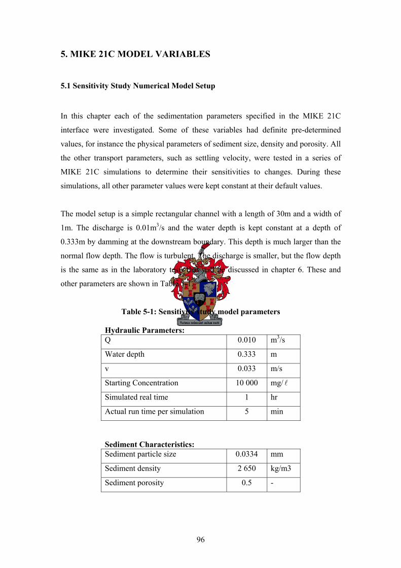
96

5. MIKE 21C MODEL VARIABLES

5.1 Sensitivity Study Numerical Model Setup

In this chapter each of the sedimentation parameters specified in the MIKE 21C

interface were investigated. Some of these variables had definite pre-determined

values, for instance the physical parameters of sediment size, density and porosity. All

the other transport parameters, such as settling velocity, were tested in a series of

MIKE 21C simulations to determine their sensitivities to changes. During these

simulations, all other parameter values were kept constant at their default values.

The model setup is a simple rectangular channel with a length of 30m and a width of

1m. The discharge is 0.01m3/s and the water depth is kept constant at a depth of

0.333m by damming at the downstream boundary. This depth is much larger than the

normal flow depth. The flow is turbulent. The discharge is smaller, but the flow depth

is the same as in the laboratory tests that will be discussed in chapter 6. These and

other parameters are shown in Table 5-1.

Table 5-1: Sensitivity study model parameters

Hydraulic Parameters: Q 0.010 m3/s

Water depth 0.333 m

v 0.033 m/s

Starting Concentration 10 000 mg/ l

Simulated real time 1 hr

Actual run time per simulation 5 min

Sediment Characteristics:

Sediment particle size 0.0334 mm

Sediment density 2 650 kg/m3

Sediment porosity 0.5 -

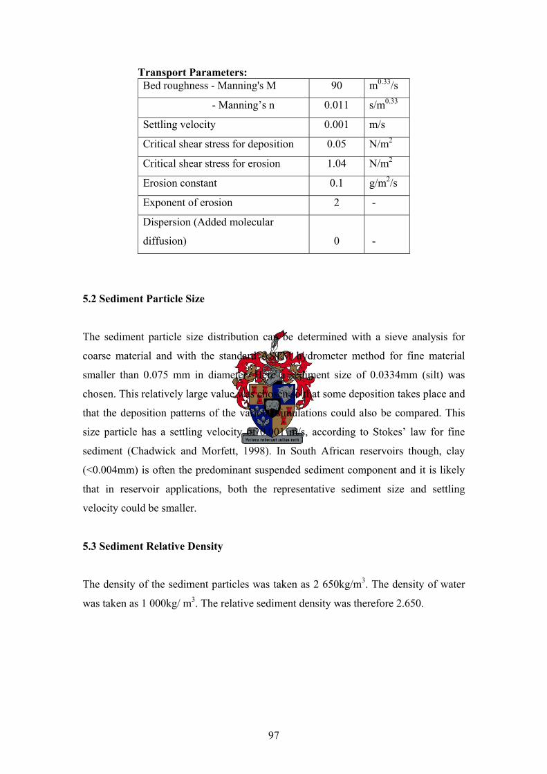
97

Transport Parameters: Bed roughness - Manning's M 90 m0.33/s

- Manning’s n 0.011 s/m0.33

Settling velocity 0.001 m/s

Critical shear stress for deposition 0.05 N/m2

Critical shear stress for erosion 1.04 N/m2

Erosion constant 0.1 g/m2/s

Exponent of erosion 2 -

Dispersion (Added molecular

diffusion) 0 -

5.2 Sediment Particle Size

The sediment particle size distribution can be determined with a sieve analysis for

coarse material and with the standard ASTM hydrometer method for fine material

smaller than 0.075 mm in diameter. Here a sediment size of 0.0334mm (silt) was

chosen. This relatively large value was chosen so that some deposition takes place and

that the deposition patterns of the various simulations could also be compared. This

size particle has a settling velocity of 0.001 m/s, according to Stokes’ law for fine

sediment (Chadwick and Morfett, 1998). In South African reservoirs though, clay

(<0.004mm) is often the predominant suspended sediment component and it is likely

that in reservoir applications, both the representative sediment size and settling

velocity could be smaller.

5.3 Sediment Relative Density

The density of the sediment particles was taken as 2 650kg/m3. The density of water

was taken as 1 000kg/ m3. The relative sediment density was therefore 2.650.

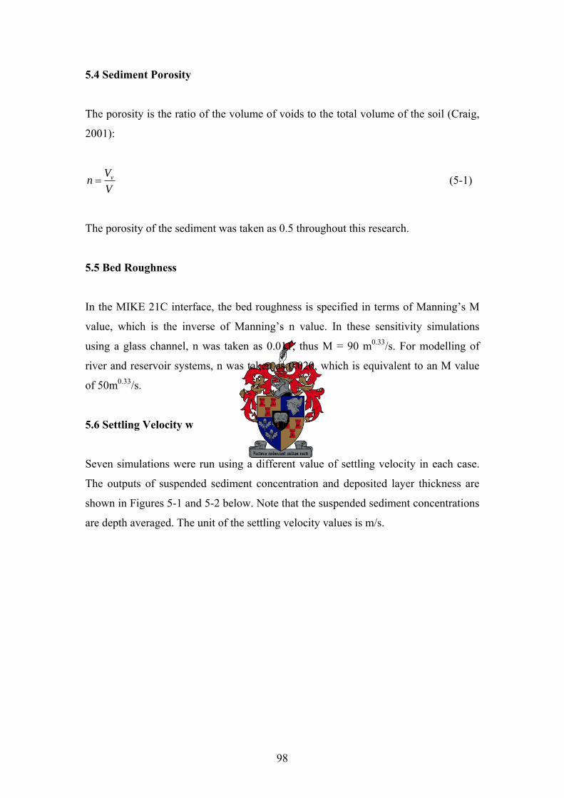
98

5.4 Sediment Porosity

The porosity is the ratio of the volume of voids to the total volume of the soil (Craig,

2001):

vVnV

= (5-1)

The porosity of the sediment was taken as 0.5 throughout this research.

5.5 Bed Roughness

In the MIKE 21C interface, the bed roughness is specified in terms of Manning’s M

value, which is the inverse of Manning’s n value. In these sensitivity simulations

using a glass channel, n was taken as 0.011, thus M = 90 m0.33/s. For modelling of

river and reservoir systems, n was taken as 0.020, which is equivalent to an M value

of 50m0.33/s.

5.6 Settling Velocity w

Seven simulations were run using a different value of settling velocity in each case.

The outputs of suspended sediment concentration and deposited layer thickness are

shown in Figures 5-1 and 5-2 below. Note that the suspended sediment concentrations

are depth averaged. The unit of the settling velocity values is m/s.

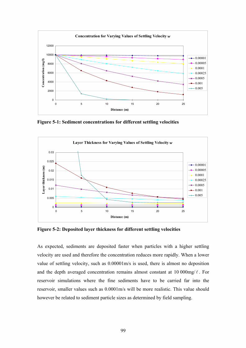
99

Concentration for Varying Values of Settling Velocity w

0

2000

4000

6000

8000

10000

12000

0 5 10 15 20 25

Distance (m)

Con

cent

ratio

n (m

g/l) 0.00001

0.000050.00010.000250.00050.0010.005

Figure 5-1: Sediment concentrations for different settling velocities

Layer Thickness for Varying Values of Settling Velocity w

0

0.005

0.01

0.015

0.02

0.025

0.03

0 5 10 15 20 25

Distance (m)

Lay

er th

ickn

ess (

m) 0.00001

0.000050.00010.000250.00050.0010.005

Figure 5-2: Deposited layer thickness for different settling velocities

As expected, sediments are deposited faster when particles with a higher settling

velocity are used and therefore the concentration reduces more rapidly. When a lower

value of settling velocity, such as 0.00001m/s is used, there is almost no deposition

and the depth averaged concentration remains almost constant at 10 000mg/ l . For

reservoir simulations where the fine sediments have to be carried far into the

reservoir, smaller values such as 0.0001m/s will be more realistic. This value should

however be related to sediment particle sizes as determined by field sampling.

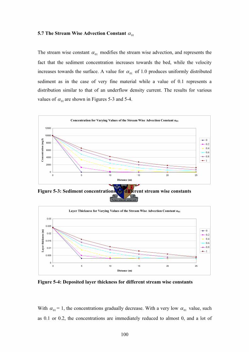
100

5.7 The Stream Wise Advection Constant 01α

The stream wise constant 01α modifies the stream wise advection, and represents the

fact that the sediment concentration increases towards the bed, while the velocity

increases towards the surface. A value for 01α of 1.0 produces uniformly distributed

sediment as in the case of very fine material while a value of 0.1 represents a

distribution similar to that of an underflow density current. The results for various

values of 01α are shown in Figures 5-3 and 5-4.

Concentration for Varying Values of the Stream Wise Advection Constant α01

0

2000

4000

6000

8000

10000

12000

0 5 10 15 20 25

Distance (m)

Con

cent

ratio

n (m

g/l) 0

0.20.40.60.81

Figure 5-3: Sediment concentrations for different stream wise constants

Layer Thickness for Varying Values of the Stream Wise Advection Constant α01

0

0.005

0.01

0.015

0.02

0.025

0.03

0 5 10 15 20 25

Distance (m)

Lay

er th

ickn

ess (

m) 0

0.20.40.60.81

Figure 5-4: Deposited layer thickness for different stream wise constants

With 01α = 1, the concentrations gradually decrease. With a very low 01α value, such

as 0.1 or 0.2, the concentrations are immediately reduced to almost 0, and a lot of

101

deposition is found at the upstream boundary (not so clear from the figure). It is

evident that for reservoir applications, a value for 01α of 1.0 is appropriate to ensure

that fine sediment is carried uniformly into the reservoir as far as possible.

5.8 Critical Shear Stress for Deposition cdτ

Deposition takes place as soon as the bed shear stress reduces to this critical shear

stress value or lower. The value of this parameter can determine whether deposition

will take place in large quantities (smaller value) or not at all (too large a value)

according to the deposition function (DHI, 2003):

1scd

D w c ττ

⎛ ⎞= ⋅ −⎜ ⎟

⎝ ⎠ (5-2)

The results for various values of cdτ are shown in Figures 5-5 and 5-6.

Concentration for Varying Values of Critical Shear Stress for Deposition

0

2000

4000

6000

8000

10000

12000

0 5 10 15 20 25

Distance (m)

Con

cent

ratio

n (m

g/l)

0.0060.0080.010.0250.050.0750.10.2

Figure 5-5: Sediment concentrations for different shear stresses for deposition

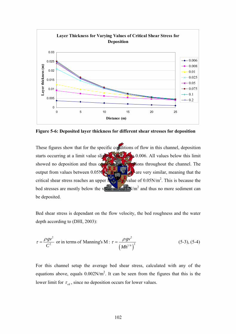
102

Layer Thickness for Varying Values of Critical Shear Stress for Deposition

0

0.005

0.01

0.015

0.02

0.025

0.03

0 5 10 15 20 25

Distance (m)

Lay

er th

ickn

ess (

m)

0.0060.0080.010.0250.050.0750.10.2

Figure 5-6: Deposited layer thickness for different shear stresses for deposition

These figures show that for the specific conditions of flow in this channel, deposition

starts occurring at a limit value slightly lower than 0.006. All values below this limit

showed no deposition and thus constant concentrations throughout the channel. The

output from values between 0.05N/m2 and 0.2N/m2 are very similar, meaning that the

critical shear stress reaches an upper limit at a value of 0.05N/m2. This is because the

bed stresses are mostly below the value of 0.05 N/m2 and thus no more sediment can

be deposited.

Bed shear stress is dependant on the flow velocity, the bed roughness and the water

depth according to (DHI, 2003):

( )2 2

22 1/ 6 or in terms of Manning's M : gv gv

C Mh

ρ ρτ τ= = (5-3), (5-4)

For this channel setup the average bed shear stress, calculated with any of the

equations above, equals 0.002N/m2. It can be seen from the figures that this is the

lower limit for cdτ , since no deposition occurs for lower values.

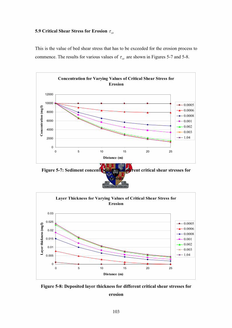
103

5.9 Critical Shear Stress for Erosion ceτ

This is the value of bed shear stress that has to be exceeded for the erosion process to

commence. The results for various values of ceτ are shown in Figures 5-7 and 5-8.

Concentration for Varying Values of Critical Shear Stress for Erosion

0

2000

4000

6000

8000

10000

12000

0 5 10 15 20 25

Distance (m)

Con

cent

ratio

n (m

g/l) 0.0005

0.00060.00080.0010.0020.0031.04

Figure 5-7: Sediment concentrations for different critical shear stresses for

erosion

Layer Thickness for Varying Values of Critical Shear Stress for Erosion

0

0.005

0.01

0.015

0.02

0.025

0.03

0 5 10 15 20 25

Distance (m)

Lay

er th

ickn

ess (

mg/

l) 0.00050.00060.00080.0010.0020.0031.04

Figure 5-8: Deposited layer thickness for different critical shear stresses for

erosion

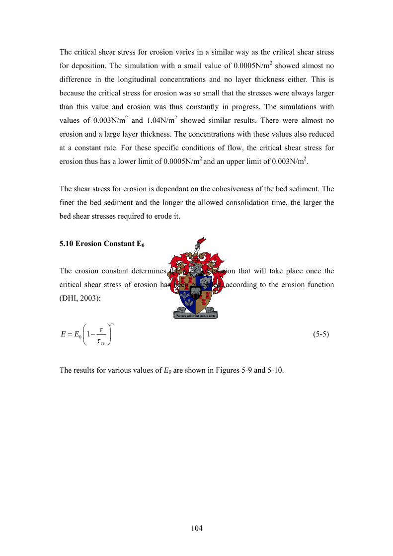
104

The critical shear stress for erosion varies in a similar way as the critical shear stress

for deposition. The simulation with a small value of 0.0005N/m2 showed almost no

difference in the longitudinal concentrations and no layer thickness either. This is

because the critical stress for erosion was so small that the stresses were always larger

than this value and erosion was thus constantly in progress. The simulations with

values of 0.003N/m2 and 1.04N/m2 showed similar results. There were almost no

erosion and a large layer thickness. The concentrations with these values also reduced

at a constant rate. For these specific conditions of flow, the critical shear stress for

erosion thus has a lower limit of 0.0005N/m2 and an upper limit of 0.003N/m2.

The shear stress for erosion is dependant on the cohesiveness of the bed sediment. The

finer the bed sediment and the longer the allowed consolidation time, the larger the

bed shear stresses required to erode it.

5.10 Erosion Constant E0

The erosion constant determines the scale of erosion that will take place once the

critical shear stress of erosion has been exceeded, according to the erosion function

(DHI, 2003):

0 1m

ce

E E ττ

⎛ ⎞= −⎜ ⎟

⎝ ⎠ (5-5)

The results for various values of E0 are shown in Figures 5-9 and 5-10.

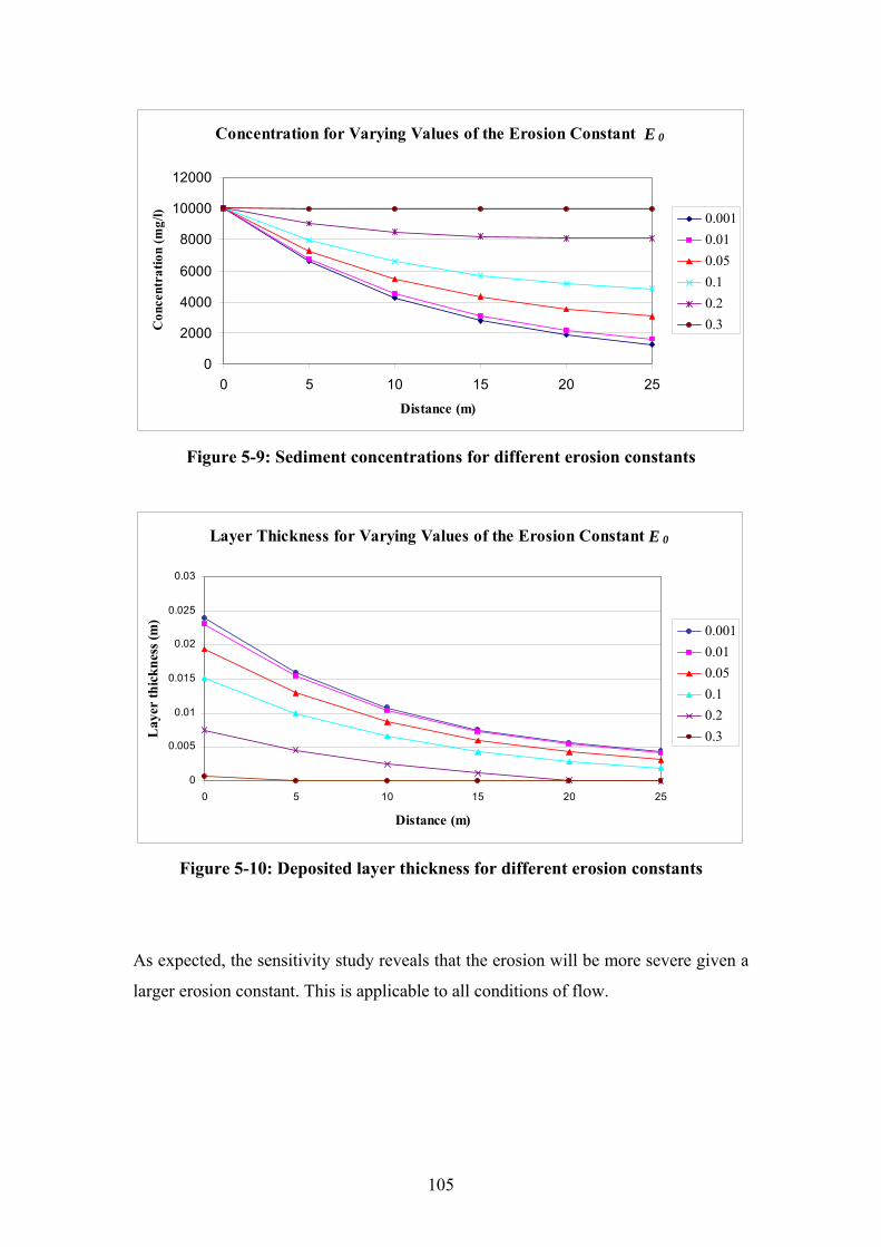
105

Concentration for Varying Values of the Erosion Constant E 0

0

2000

4000

6000

8000

10000

12000

0 5 10 15 20 25

Distance (m)

Con

cent

ratio

n (m

g/l) 0.001

0.010.050.10.20.3

Figure 5-9: Sediment concentrations for different erosion constants

Layer Thickness for Varying Values of the Erosion Constant E 0

0

0.005

0.01

0.015

0.02

0.025

0.03

0 5 10 15 20 25

Distance (m)

Lay

er th

ickn

ess (

m)

0.0010.010.050.10.20.3

Figure 5-10: Deposited layer thickness for different erosion constants

As expected, the sensitivity study reveals that the erosion will be more severe given a

larger erosion constant. This is applicable to all conditions of flow.

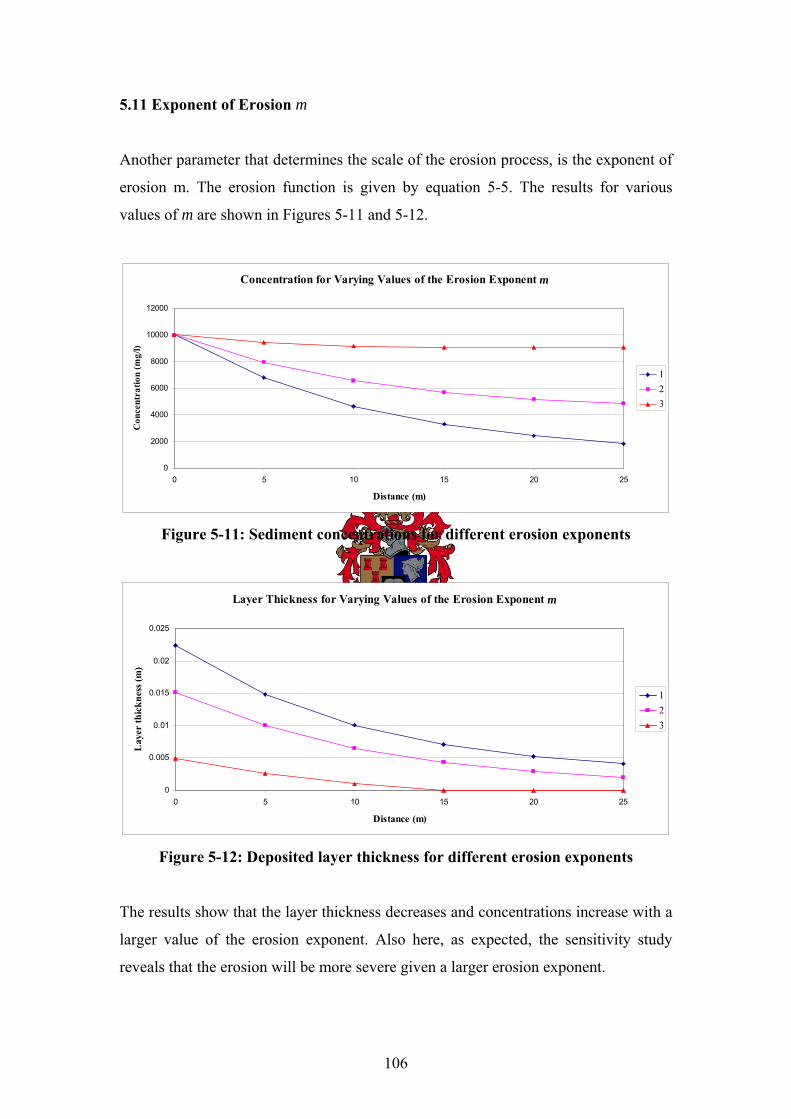
106

5.11 Exponent of Erosion m

Another parameter that determines the scale of the erosion process, is the exponent of

erosion m. The erosion function is given by equation 5-5. The results for various

values of m are shown in Figures 5-11 and 5-12.

Concentration for Varying Values of the Erosion Exponent m

0

2000

4000

6000

8000

10000

12000

0 5 10 15 20 25

Distance (m)

Con

cent

ratio

n (m

g/l)

123

Figure 5-11: Sediment concentrations for different erosion exponents

Layer Thickness for Varying Values of the Erosion Exponent m

0

0.005

0.01

0.015

0.02

0.025

0 5 10 15 20 25

Distance (m)

Lay

er th

ickn

ess (

m)

123

Figure 5-12: Deposited layer thickness for different erosion exponents

The results show that the layer thickness decreases and concentrations increase with a

larger value of the erosion exponent. Also here, as expected, the sensitivity study

reveals that the erosion will be more severe given a larger erosion exponent.

107

5.12 Dispersion

This parameter specifies the amount of added molecular diffusion required for the

simulation. For all simulations in this research, this parameter is kept at a constant

value of 0. The molecular diffusion has very little effect on the overall dispersion. The

x and y horizontal dispersion coefficients are determined by the model itself (DHI,

2003).

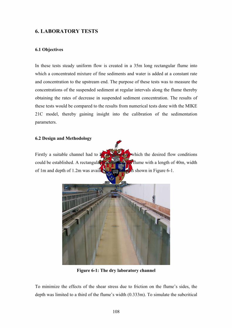
108

6. LABORATORY TESTS

6.1 Objectives

In these tests steady uniform flow is created in a 35m long rectangular flume into

which a concentrated mixture of fine sediments and water is added at a constant rate

and concentration to the upstream end. The purpose of these tests was to measure the

concentrations of the suspended sediment at regular intervals along the flume thereby

obtaining the rates of decrease in suspended sediment concentration. The results of

these tests would be compared to the results from numerical tests done with the MIKE

21C model, thereby gaining insight into the calibration of the sedimentation

parameters.

6.2 Design and Methodology

Firstly a suitable channel had to be identified in which the desired flow conditions

could be established. A rectangular horizontal glass flume with a length of 40m, width

of 1m and depth of 1.2m was available. The flume is shown in Figure 6-1.

Figure 6-1: The dry laboratory channel

To minimize the effects of the shear stress due to friction on the flume’s sides, the

depth was limited to a third of the flume’s width (0.333m). To simulate the subcritical

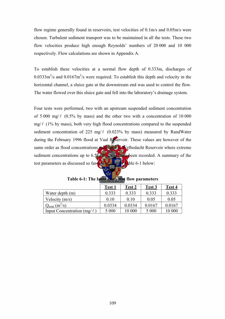
109

flow regime generally found in reservoirs, test velocities of 0.1m/s and 0.05m/s were

chosen. Turbulent sediment transport was to be maintained in all the tests. These two

flow velocities produce high enough Reynolds’ numbers of 20 000 and 10 000

respectively. Flow calculations are shown in Appendix A.

To establish these velocities at a normal flow depth of 0.333m, discharges of

0.0333m3/s and 0.0167m3/s were required. To establish this depth and velocity in the

horizontal channel, a sluice gate at the downstream end was used to control the flow.

The water flowed over this sluice gate and fell into the laboratory’s drainage system.

Four tests were performed, two with an upstream suspended sediment concentration

of 5 000 mg/ l (0.5% by mass) and the other two with a concentration of 10 000

mg/ l (1% by mass), both very high flood concentrations compared to the suspended

sediment concentration of 225 mg/ l (0.023% by mass) measured by RandWater

during the February 1996 flood at Vaal Reservoir. These values are however of the

same order as flood concentrations measured at Welbedacht Reservoir where extreme

sediment concentrations up to 6.5% by mass have been recorded. A summary of the

test parameters as discussed so far can be seen in Table 6-1 below:

Table 6-1: The laboratory test flow parameters

Test 1 Test 2 Test 3 Test 4 Water depth (m) 0.333 0.333 0.333 0.333 Velocity (m/s) 0.10 0.10 0.05 0.05 Qtotal (m3/s) 0.0334 0.0334 0.0167 0.0167 Input Concentration (mg/ l ) 5 000 10 000 5 000 10 000

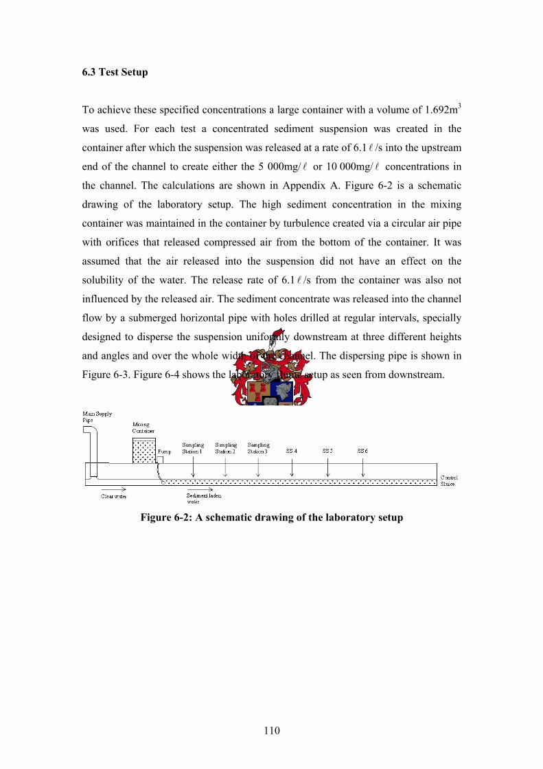
110

6.3 Test Setup

To achieve these specified concentrations a large container with a volume of 1.692m3

was used. For each test a concentrated sediment suspension was created in the

container after which the suspension was released at a rate of 6.1l /s into the upstream

end of the channel to create either the 5 000mg/ l or 10 000mg/ l concentrations in

the channel. The calculations are shown in Appendix A. Figure 6-2 is a schematic

drawing of the laboratory setup. The high sediment concentration in the mixing

container was maintained in the container by turbulence created via a circular air pipe

with orifices that released compressed air from the bottom of the container. It was

assumed that the air released into the suspension did not have an effect on the

solubility of the water. The release rate of 6.1 l /s from the container was also not

influenced by the released air. The sediment concentrate was released into the channel

flow by a submerged horizontal pipe with holes drilled at regular intervals, specially

designed to disperse the suspension uniformly downstream at three different heights

and angles and over the whole width of the channel. The dispersing pipe is shown in

Figure 6-3. Figure 6-4 shows the laboratory flume setup as seen from downstream.

Figure 6-2: A schematic drawing of the laboratory setup

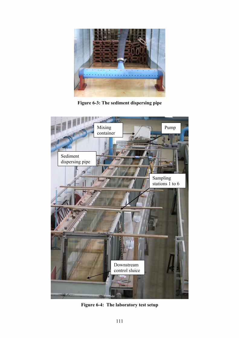
111

Figure 6-3: The sediment dispersing pipe

Figure 6-4: The laboratory test setup

Mixing container

Downstream control sluice

Sampling stations 1 to 6

Pump

Sediment dispersing pipe

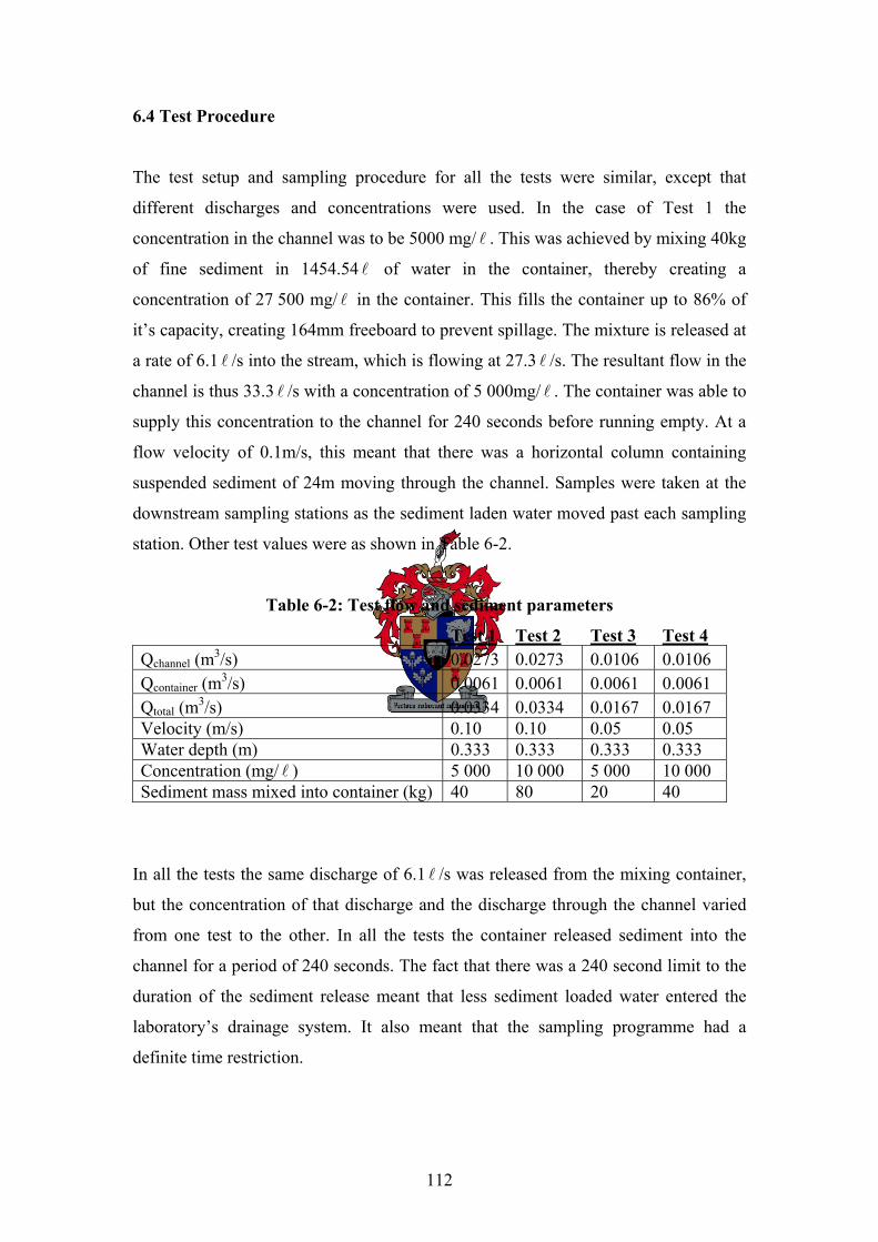
112

6.4 Test Procedure

The test setup and sampling procedure for all the tests were similar, except that

different discharges and concentrations were used. In the case of Test 1 the

concentration in the channel was to be 5000 mg/ l . This was achieved by mixing 40kg

of fine sediment in 1454.54 l of water in the container, thereby creating a

concentration of 27 500 mg/ l in the container. This fills the container up to 86% of

it’s capacity, creating 164mm freeboard to prevent spillage. The mixture is released at

a rate of 6.1 l /s into the stream, which is flowing at 27.3 l /s. The resultant flow in the

channel is thus 33.3 l /s with a concentration of 5 000mg/ l . The container was able to

supply this concentration to the channel for 240 seconds before running empty. At a

flow velocity of 0.1m/s, this meant that there was a horizontal column containing

suspended sediment of 24m moving through the channel. Samples were taken at the

downstream sampling stations as the sediment laden water moved past each sampling

station. Other test values were as shown in Table 6-2.

Table 6-2: Test flow and sediment parameters

Test 1 Test 2 Test 3 Test 4 Qchannel (m3/s) 0.0273 0.0273 0.0106 0.0106 Qcontainer (m3/s) 0.0061 0.0061 0.0061 0.0061 Qtotal (m3/s) 0.0334 0.0334 0.0167 0.0167 Velocity (m/s) 0.10 0.10 0.05 0.05 Water depth (m) 0.333 0.333 0.333 0.333 Concentration (mg/ l ) 5 000 10 000 5 000 10 000 Sediment mass mixed into container (kg) 40 80 20 40

In all the tests the same discharge of 6.1l /s was released from the mixing container,

but the concentration of that discharge and the discharge through the channel varied

from one test to the other. In all the tests the container released sediment into the

channel for a period of 240 seconds. The fact that there was a 240 second limit to the

duration of the sediment release meant that less sediment loaded water entered the

laboratory’s drainage system. It also meant that the sampling programme had a

definite time restriction.

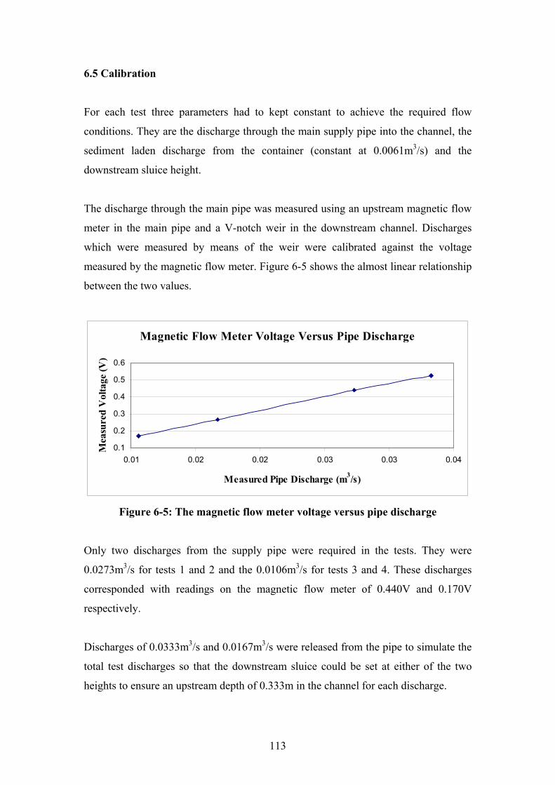
113

6.5 Calibration

For each test three parameters had to kept constant to achieve the required flow

conditions. They are the discharge through the main supply pipe into the channel, the

sediment laden discharge from the container (constant at 0.0061m3/s) and the

downstream sluice height.

The discharge through the main pipe was measured using an upstream magnetic flow

meter in the main pipe and a V-notch weir in the downstream channel. Discharges

which were measured by means of the weir were calibrated against the voltage

measured by the magnetic flow meter. Figure 6-5 shows the almost linear relationship

between the two values.

Magnetic Flow Meter Voltage Versus Pipe Discharge

0.1

0.2

0.3

0.4

0.5

0.6

0.01 0.02 0.02 0.03 0.03 0.04

Measured Pipe Discharge (m3/s)

Mea

sure

d V

olta

ge (V

)

Figure 6-5: The magnetic flow meter voltage versus pipe discharge

Only two discharges from the supply pipe were required in the tests. They were

0.0273m3/s for tests 1 and 2 and the 0.0106m3/s for tests 3 and 4. These discharges

corresponded with readings on the magnetic flow meter of 0.440V and 0.170V

respectively.

Discharges of 0.0333m3/s and 0.0167m3/s were released from the pipe to simulate the

total test discharges so that the downstream sluice could be set at either of the two

heights to ensure an upstream depth of 0.333m in the channel for each discharge.

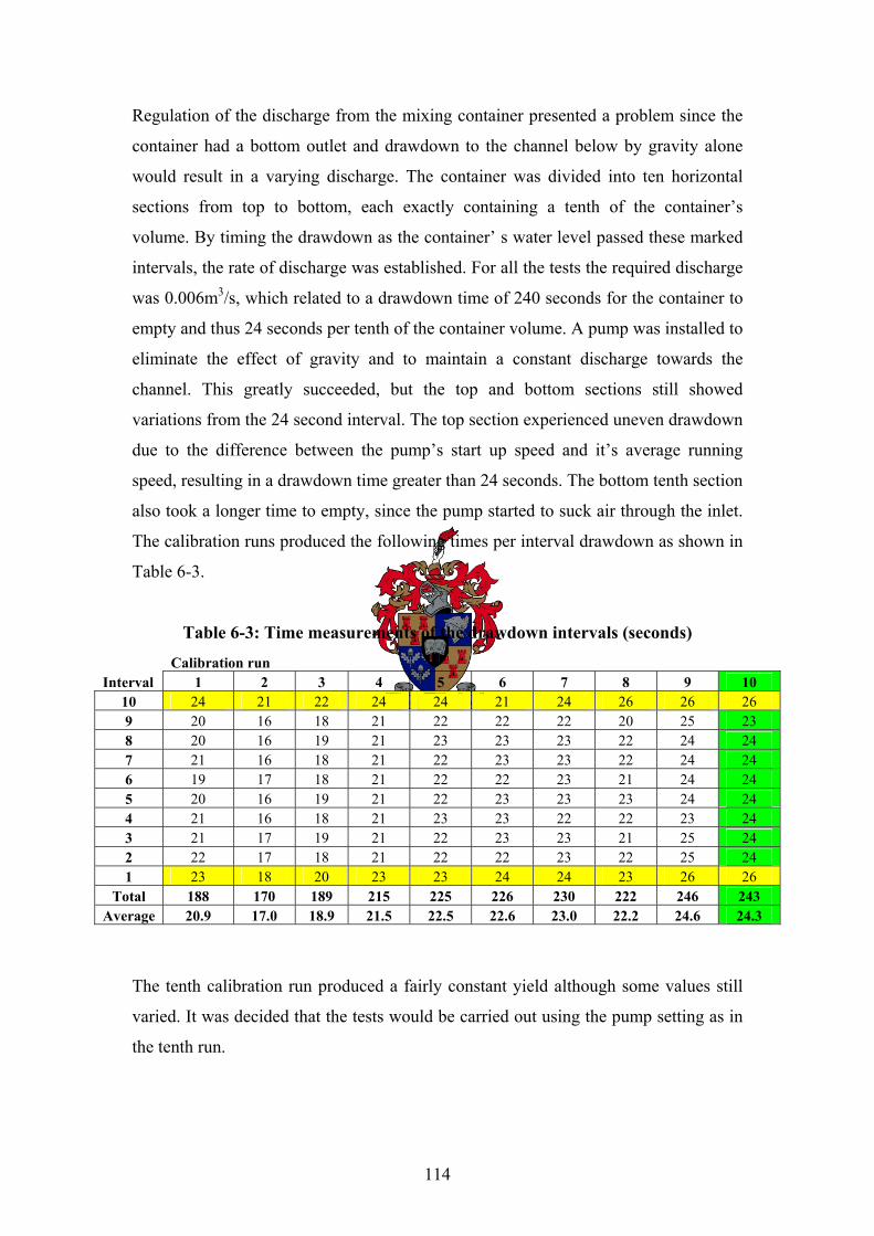
114

Regulation of the discharge from the mixing container presented a problem since the

container had a bottom outlet and drawdown to the channel below by gravity alone

would result in a varying discharge. The container was divided into ten horizontal

sections from top to bottom, each exactly containing a tenth of the container’s

volume. By timing the drawdown as the container’ s water level passed these marked

intervals, the rate of discharge was established. For all the tests the required discharge

was 0.006m3/s, which related to a drawdown time of 240 seconds for the container to

empty and thus 24 seconds per tenth of the container volume. A pump was installed to

eliminate the effect of gravity and to maintain a constant discharge towards the

channel. This greatly succeeded, but the top and bottom sections still showed

variations from the 24 second interval. The top section experienced uneven drawdown

due to the difference between the pump’s start up speed and it’s average running

speed, resulting in a drawdown time greater than 24 seconds. The bottom tenth section

also took a longer time to empty, since the pump started to suck air through the inlet.

The calibration runs produced the following times per interval drawdown as shown in

Table 6-3.

Table 6-3: Time measurements of the drawdown intervals (seconds)

Calibration run Interval 1 2 3 4 5 6 7 8 9 10

10 24 21 22 24 24 21 24 26 26 26 9 20 16 18 21 22 22 22 20 25 23 8 20 16 19 21 23 23 23 22 24 24 7 21 16 18 21 22 23 23 22 24 24 6 19 17 18 21 22 22 23 21 24 24 5 20 16 19 21 22 23 23 23 24 24 4 21 16 18 21 23 23 22 22 23 24 3 21 17 19 21 22 23 23 21 25 24 2 22 17 18 21 22 22 23 22 25 24 1 23 18 20 23 23 24 24 23 26 26

Total 188 170 189 215 225 226 230 222 246 243 Average 20.9 17.0 18.9 21.5 22.5 22.6 23.0 22.2 24.6 24.3

The tenth calibration run produced a fairly constant yield although some values still

varied. It was decided that the tests would be carried out using the pump setting as in

the tenth run.

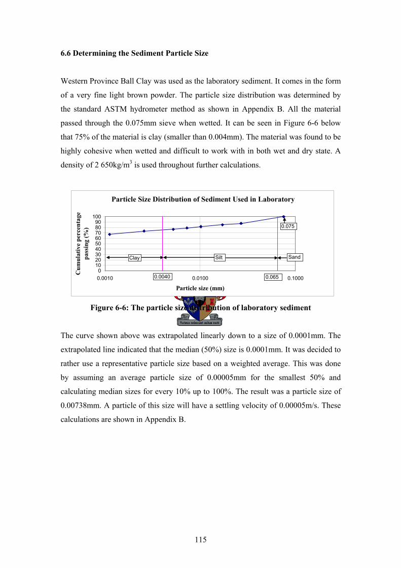
115

6.6 Determining the Sediment Particle Size

Western Province Ball Clay was used as the laboratory sediment. It comes in the form

of a very fine light brown powder. The particle size distribution was determined by

the standard ASTM hydrometer method as shown in Appendix B. All the material

passed through the 0.075mm sieve when wetted. It can be seen in Figure 6-6 below

that 75% of the material is clay (smaller than 0.004mm). The material was found to be

highly cohesive when wetted and difficult to work with in both wet and dry state. A

density of 2 650kg/m3 is used throughout further calculations.

Figure 6-6: The particle size distribution of laboratory sediment

The curve shown above was extrapolated linearly down to a size of 0.0001mm. The

extrapolated line indicated that the median (50%) size is 0.0001mm. It was decided to

rather use a representative particle size based on a weighted average. This was done

by assuming an average particle size of 0.00005mm for the smallest 50% and

calculating median sizes for every 10% up to 100%. The result was a particle size of

0.00738mm. A particle of this size will have a settling velocity of 0.00005m/s. These

calculations are shown in Appendix B.

Particle Size Distribution of Sediment Used in Laboratory

0102030405060708090

100

0.0010 0.0100 0.1000

Particle size (mm)

Cum

ulat

ive

perc

enta

ge

pass

ing

(%)

SiltClay

0.0040

Sand

0.065

0.075

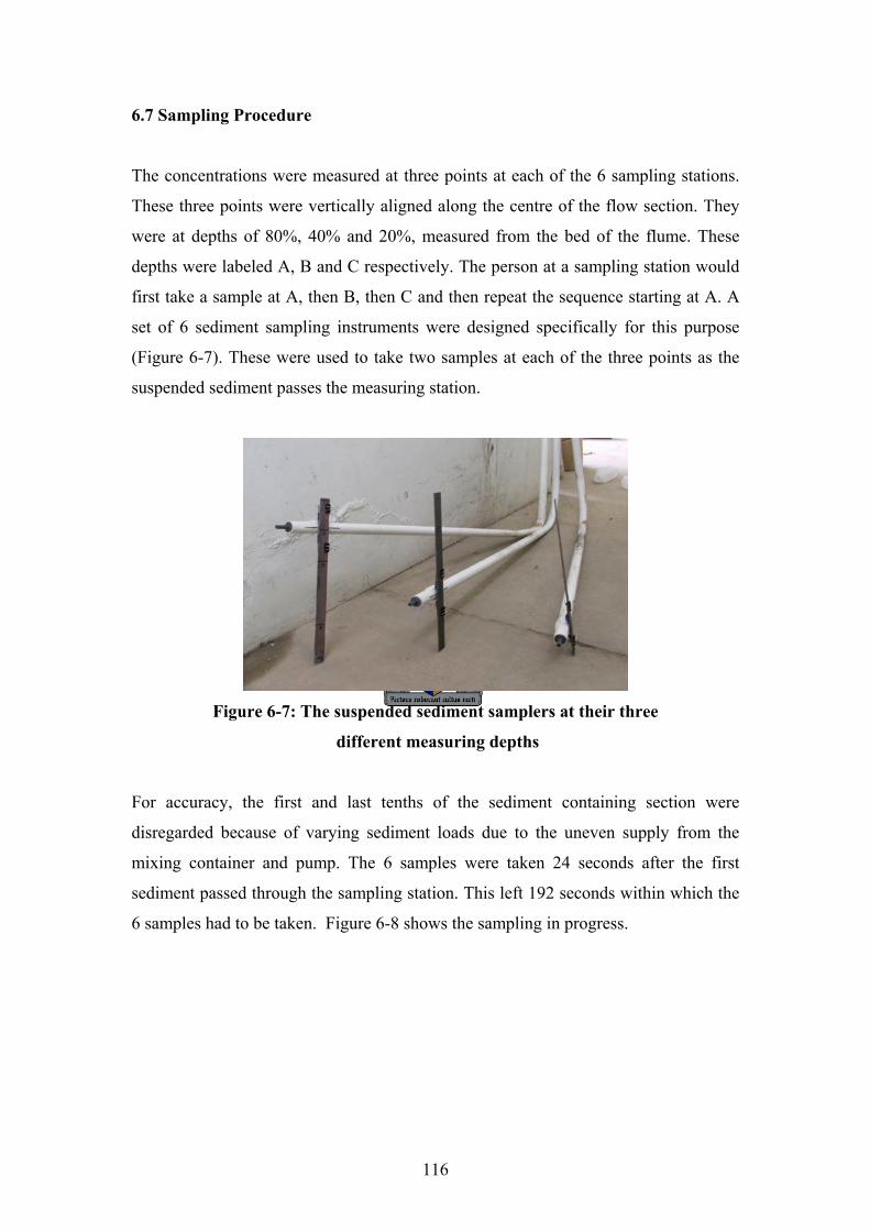
116

6.7 Sampling Procedure

The concentrations were measured at three points at each of the 6 sampling stations.

These three points were vertically aligned along the centre of the flow section. They

were at depths of 80%, 40% and 20%, measured from the bed of the flume. These

depths were labeled A, B and C respectively. The person at a sampling station would

first take a sample at A, then B, then C and then repeat the sequence starting at A. A

set of 6 sediment sampling instruments were designed specifically for this purpose

(Figure 6-7). These were used to take two samples at each of the three points as the

suspended sediment passes the measuring station.

Figure 6-7: The suspended sediment samplers at their three

different measuring depths

For accuracy, the first and last tenths of the sediment containing section were

disregarded because of varying sediment loads due to the uneven supply from the

mixing container and pump. The 6 samples were taken 24 seconds after the first

sediment passed through the sampling station. This left 192 seconds within which the

6 samples had to be taken. Figure 6-8 shows the sampling in progress.

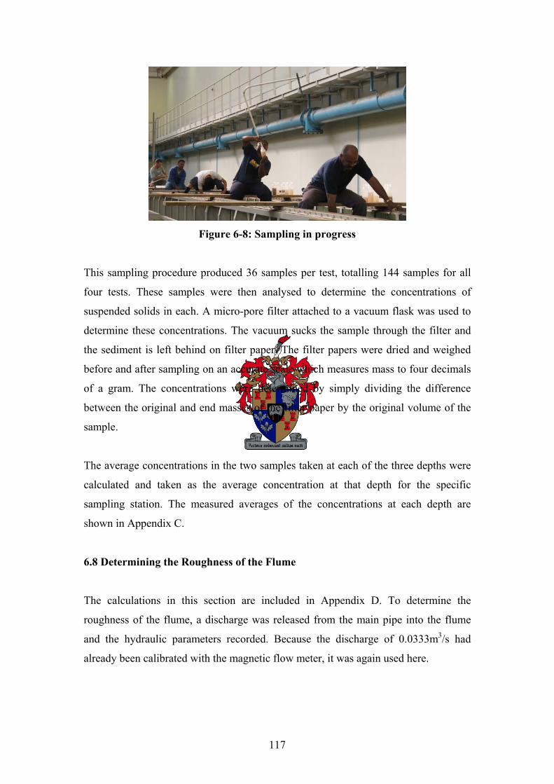
117

Figure 6-8: Sampling in progress

This sampling procedure produced 36 samples per test, totalling 144 samples for all

four tests. These samples were then analysed to determine the concentrations of

suspended solids in each. A micro-pore filter attached to a vacuum flask was used to

determine these concentrations. The vacuum sucks the sample through the filter and

the sediment is left behind on filter paper. The filter papers were dried and weighed

before and after sampling on an accurate scale which measures mass to four decimals

of a gram. The concentrations were determined by simply dividing the difference

between the original and end masses of the filter paper by the original volume of the

sample.

The average concentrations in the two samples taken at each of the three depths were

calculated and taken as the average concentration at that depth for the specific

sampling station. The measured averages of the concentrations at each depth are

shown in Appendix C.

6.8 Determining the Roughness of the Flume

The calculations in this section are included in Appendix D. To determine the

roughness of the flume, a discharge was released from the main pipe into the flume

and the hydraulic parameters recorded. Because the discharge of 0.0333m3/s had

already been calibrated with the magnetic flow meter, it was again used here.

118

With a discharge at 0.0333m3/s, the upstream and downstream flow depths varied by

25mm over a length of 30m. The Reynold’s number for these conditions was

calculated as 28 800, which meant that the flow was turbulent.

The channel’s Manning n value was found to be 0.0114 by using frictional energy loss

equations. This value was substituted into Manning’s equation and the discharge,

which uniform flow at this average depth would produce, was calculated. To solve for

the absolute roughness coefficient ks, this discharge was set equal to the equation for

discharge of turbulent flow, shown below. The value of ks was found to be 0.00038m.

125.75 log 3.3s

RQ A gRsk

gRsυ

⎡ ⎤⎢ ⎥⎢ ⎥= ⋅⎢ ⎥+⎢ ⎥⎣ ⎦

(6-1)

9.32 30gRs kυ

⋅= < (6-2)

The value of the parameter above was calculated to be smaller than 30. This meant

that the flow was smooth turbulent, and that in fact it was necessary to calculate the

values of n and ks with the methods above, and not by direct methods such as Figure

3-8 (Rooseboom and van Zyl, 1978) of the SANRAL Road Drainage Manual.

6.9 The Vertical Velocity Profiles for the Test Conditions

The Reynolds’ numbers for all the test conditions were found to be larger than 2 000,

thus the flow conditions in all the laboratory tests were turbulent.

3

1000*0.2*0.1Test 1&2) Re 20008 20001.003*10

RVρμ −= = = > (6-3)

3

1000*0.2*0.05Test 3&4) Re 10004 20001.003*10

RVρμ −= = = > (6-4)

119

The vertical velocity profile for turbulent flow is given by:

0

2 .ln ygDsy

v π⎛ ⎞⎜ ⎟⎝ ⎠

= (6-5)

For all the tests, 0y was found to be 1.296 *10-5 by the equation:

00 29.6 14.8

sk Ry = = (6-6)

where: sk = 0.000384 and thus 0R = 0.000192. Laboratory test conditions required significant damming of the flow. The differences

in water levels between the upstream and downstream channel ends were too small to

be measured. Energy principles could thus not be used to determine the energy slope

accurately. Values of s , the energy slope, were determined through trial and error

until the average velocity for the tests was reached. The average velocity for turbulent

flow is given by:

0

5.55.75 log Dv gDsR

⎛ ⎞= ⋅ ⋅ ⎜ ⎟

⎝ ⎠ (6-7)

For Tests 1 and 2, a value of 0.00000584m/m was used for s in the equation for the

velocity profile. For Tests 3 and 4, the value of s was 0.00000146m/m. These values

corresponded with average velocities of 0.1 and 0.05 m/s respectively. The

calculations are shown in Appendix E. The calculated velocity profiles are shown in

Figures 6-9 and 6-10.

120

Turbulent Vertical Velocity Distribution for Tests 1 and 2

0.000.050.100.150.200.250.300.35

0.04 0.06 0.08 0.10 0.12

Velocity (m/s)

Hei

ght f

rom

bed

(m)

Velocity profileDepth ADepth BDepth CSurface

Figure 6-9: The calculated velocity profile for Tests 1 and 2, with an average

velocity of 0.1 m/s

Turbulent Vertical Velocity Distribution for Tests 3 and 4

0.000.050.100.150.200.250.300.35

0.01 0.02 0.03 0.04 0.05 0.06

Velocity (m/s)

Hei

ght f

rom

bed

(m)

Velocity profileDepth ADepth BDepth CSurface

Figure 6-10: The calculated velocity profile for Tests 3 and 4, with an average

velocity of 0.05 m/s

The velocities at each of the three depths were also calculated and these velocities

were used to calculate a single value of concentration at each of the sampling stations

on a weighted average basis. Each of the sampling stations was thus linked to only

one depth integrated value of sediment concentration. This made the results of the

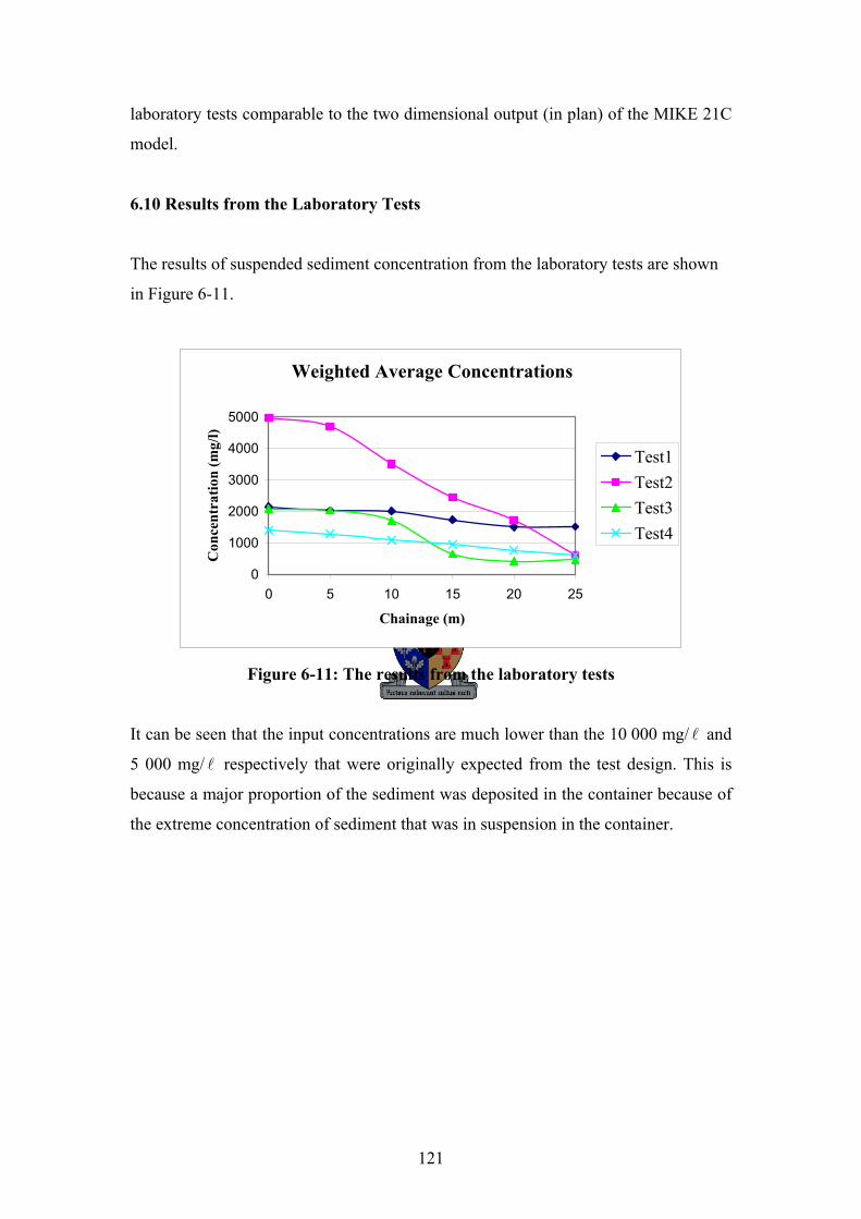
121

laboratory tests comparable to the two dimensional output (in plan) of the MIKE 21C

model.

6.10 Results from the Laboratory Tests The results of suspended sediment concentration from the laboratory tests are shown

in Figure 6-11.

Weighted Average Concentrations

0

1000

2000

3000

4000

5000

0 5 10 15 20 25

Chainage (m)

Con

cent

ratio

n (m

g/l)

Test1Test2Test3Test4

Figure 6-11: The results from the laboratory tests

It can be seen that the input concentrations are much lower than the 10 000 mg/ l and

5 000 mg/ l respectively that were originally expected from the test design. This is

because a major proportion of the sediment was deposited in the container because of

the extreme concentration of sediment that was in suspension in the container.

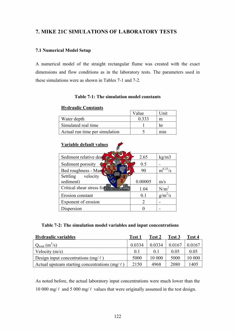
122

7. MIKE 21C SIMULATIONS OF LABORATORY TESTS

7.1 Numerical Model Setup

A numerical model of the straight rectangular flume was created with the exact

dimensions and flow conditions as in the laboratory tests. The parameters used in

these simulations were as shown in Tables 7-1 and 7-2.

Table 7-1: The simulation model constants

Hydraulic Constants Value Unit Water depth 0.333 m Simulated real time 1 hr Actual run time per simulation 5 min Variable default values Sediment relative density 2.65 kg/m3 Sediment porosity 0.5 - Bed roughness - Manning's M 90 m0.33/s Settling velocity (laboratory sediment) 0.00005 m/s Critical shear stress for erosion ceτ 1.04 N/m2 Erosion constant 0.1 g/m2/s Exponent of erosion 2 - Dispersion 0 -

Table 7-2: The simulation model variables and input concentrations Hydraulic variables Test 1 Test 2 Test 3 Test 4

Qtotal (m3/s) 0.0334 0.0334 0.0167 0.0167Velocity (m/s) 0.1 0.1 0.05 0.05 Design input concentrations (mg/ l ) 5000 10 000 5000 10 000Actual upsteam starting concentrations (mg/ l ) 2150 4968 2080 1405 As noted before, the actual laboratory input concentrations were much lower than the

10 000 mg/ l and 5 000 mg/ l values that were originally assumed in the test design.

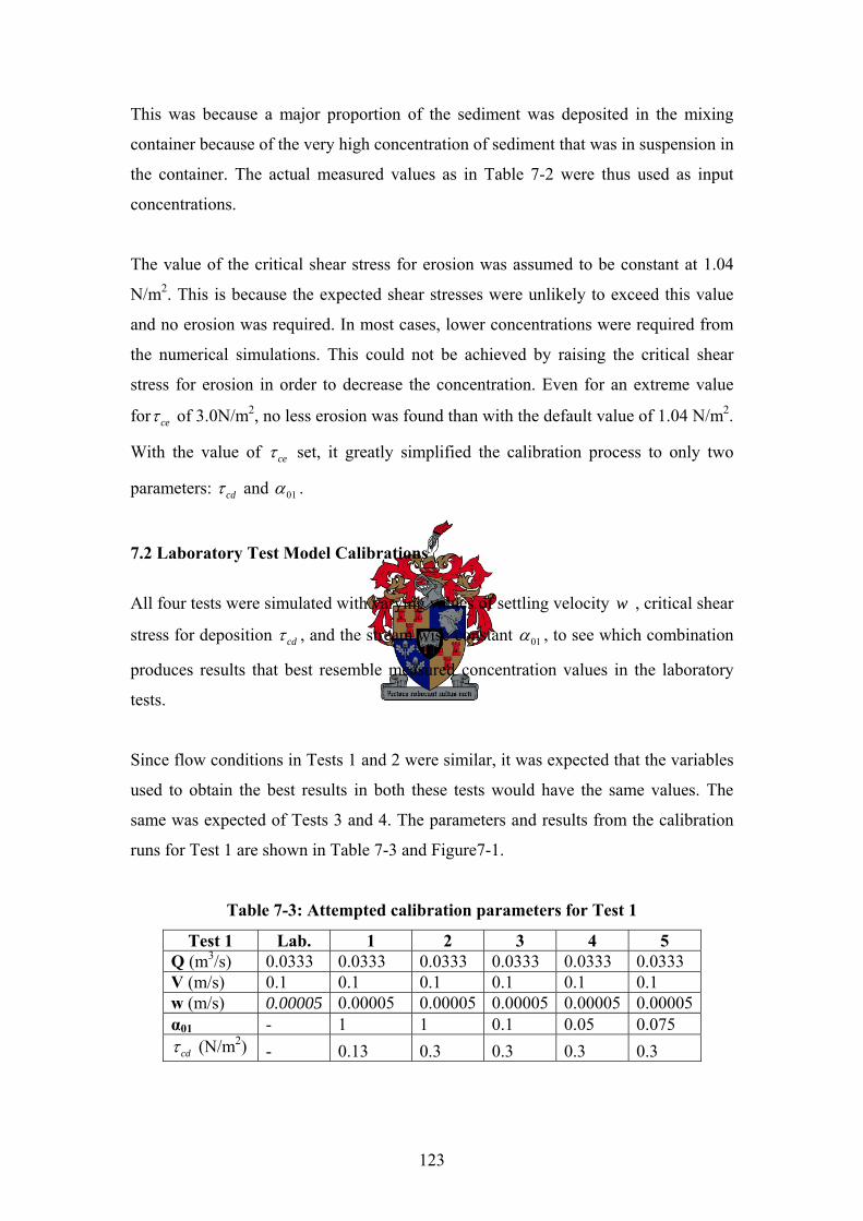
123

This was because a major proportion of the sediment was deposited in the mixing

container because of the very high concentration of sediment that was in suspension in

the container. The actual measured values as in Table 7-2 were thus used as input

concentrations.

The value of the critical shear stress for erosion was assumed to be constant at 1.04

N/m2. This is because the expected shear stresses were unlikely to exceed this value

and no erosion was required. In most cases, lower concentrations were required from

the numerical simulations. This could not be achieved by raising the critical shear

stress for erosion in order to decrease the concentration. Even for an extreme value

for ceτ of 3.0N/m2, no less erosion was found than with the default value of 1.04 N/m2.

With the value of ceτ set, it greatly simplified the calibration process to only two

parameters: cdτ and 01α .

7.2 Laboratory Test Model Calibrations

All four tests were simulated with varying values of settling velocity w , critical shear

stress for deposition cdτ , and the stream wise constant 01α , to see which combination

produces results that best resemble measured concentration values in the laboratory

tests.

Since flow conditions in Tests 1 and 2 were similar, it was expected that the variables

used to obtain the best results in both these tests would have the same values. The

same was expected of Tests 3 and 4. The parameters and results from the calibration

runs for Test 1 are shown in Table 7-3 and Figure7-1.

Table 7-3: Attempted calibration parameters for Test 1

Test 1 Lab. 1 2 3 4 5 Q (m3/s) 0.0333 0.0333 0.0333 0.0333 0.0333 0.0333 V (m/s) 0.1 0.1 0.1 0.1 0.1 0.1 w (m/s) 0.00005 0.00005 0.00005 0.00005 0.00005 0.00005 α01 - 1 1 0.1 0.05 0.075

cdτ (N/m2) - 0.13 0.3 0.3 0.3 0.3

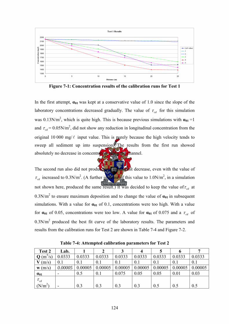
124

Test 1 Results

1300

1400

1500

1600

1700

1800

1900

2000

2100

2200

0 5 10 15 20 25

Distance (m)

Con

cent

ratio

n (m

g/l) Lab values

12345

Figure 7-1: Concentration results of the calibration runs for Test 1

In the first attempt, α01 was kept at a conservative value of 1.0 since the slope of the

laboratory concentrations decreased gradually. The value of cdτ for this simulation

was 0.13N/m2, which is quite high. This is because previous simulations with α01 =1

and cdτ = 0.05N/m2, did not show any reduction in longitudinal concentration from the

original 10 000 mg/ l input value. This is purely because the high velocity tends to

sweep all sediment up into suspension. The results from the first run showed

absolutely no decrease in concentration along the channel.

The second run also did not produce any significant decrease, even with the value of

cdτ increased to 0.3N/m2. (A further increase of this value to 1.0N/m2, in a simulation

not shown here, produced the same result.) It was decided to keep the value of cdτ at

0.3N/m2 to ensure maximum deposition and to change the value of α01 in subsequent

simulations. With a value for α01 of 0.1, concentrations were too high. With a value

for α01 of 0.05, concentrations were too low. A value for α01 of 0.075 and a cdτ of

0.3N/m2 produced the best fit curve of the laboratory results. The parameters and

results from the calibration runs for Test 2 are shown in Table 7-4 and Figure 7-2.

Table 7-4: Attempted calibration parameters for Test 2

Test 2 Lab. 1 2 3 4 5 6 7 Q (m3/s) 0.0333 0.0333 0.0333 0.0333 0.0333 0.0333 0.0333 0.0333 V (m/s) 0.1 0.1 0.1 0.1 0.1 0.1 0.1 0.1 w (m/s) 0.00005 0.00005 0.00005 0.00005 0.00005 0.00005 0.00005 0.00005α01 - 0.5 0.1 0.075 0.05 0.05 0.01 0.03

cdτ (N/m2) - 0.3 0.3 0.3 0.3 0.5 0.5 0.5

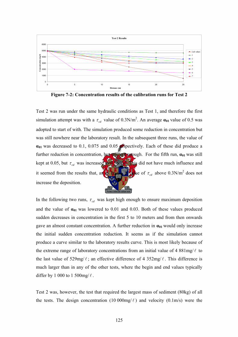
125

Test 2 Results

0

1000

2000

3000

4000

5000

6000

0 5 10 15 20 25

Distance (m)

Con

cent

ratio

n (m

g/l)

Lab values

1

2

3

4

5

6

7

Figure 7-2: Concentration results of the calibration runs for Test 2

Test 2 was run under the same hydraulic conditions as Test 1, and therefore the first

simulation attempt was with a cdτ value of 0.3N/m2. An average α01 value of 0.5 was

adopted to start of with. The simulation produced some reduction in concentration but

was still nowhere near the laboratory result. In the subsequent three runs, the value of

α01 was decreased to 0.1, 0.075 and 0.05 respectively. Each of these did produce a

further reduction in concentration, but still not enough. For the fifth run, α01 was still

kept at 0.05, but cdτ was increased to 0.5N/m2. This did not have much influence and

it seemed from the results that, as in Test 1, a value of cdτ above 0.3N/m2 does not

increase the deposition.

In the following two runs, cdτ was kept high enough to ensure maximum deposition

and the value of α01 was lowered to 0.01 and 0.03. Both of these values produced

sudden decreases in concentration in the first 5 to 10 meters and from then onwards

gave an almost constant concentration. A further reduction in α01 would only increase

the initial sudden concentration reduction. It seems as if the simulation cannot

produce a curve similar to the laboratory results curve. This is most likely because of

the extreme range of laboratory concentrations from an initial value of 4 881mg/ l to

the last value of 529mg/ l ; an effective difference of 4 352mg/ l . This difference is

much larger than in any of the other tests, where the begin and end values typically

differ by 1 000 to 1 500mg/ l .

Test 2 was, however, the test that required the largest mass of sediment (80kg) of all

the tests. The design concentration (10 000mg/ l ) and velocity (0.1m/s) were the

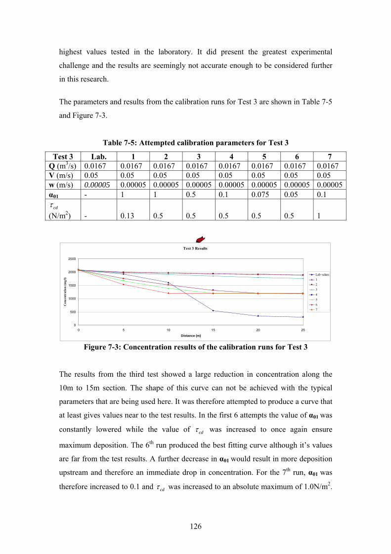
126

highest values tested in the laboratory. It did present the greatest experimental

challenge and the results are seemingly not accurate enough to be considered further

in this research.

The parameters and results from the calibration runs for Test 3 are shown in Table 7-5

and Figure 7-3.

Table 7-5: Attempted calibration parameters for Test 3

Test 3 Lab. 1 2 3 4 5 6 7 Q (m3/s) 0.0167 0.0167 0.0167 0.0167 0.0167 0.0167 0.0167 0.0167 V (m/s) 0.05 0.05 0.05 0.05 0.05 0.05 0.05 0.05 w (m/s) 0.00005 0.00005 0.00005 0.00005 0.00005 0.00005 0.00005 0.00005α01 - 1 1 0.5 0.1 0.075 0.05 0.1

cdτ (N/m2) - 0.13 0.5 0.5 0.5 0.5 0.5 1

Test 3 Results

0

500

1000

1500

2000

2500

0 5 10 15 20 25

Distance (m)

Con

cent

ratio

n (m

g/l)

Lab values1234567

Figure 7-3: Concentration results of the calibration runs for Test 3

The results from the third test showed a large reduction in concentration along the

10m to 15m section. The shape of this curve can not be achieved with the typical

parameters that are being used here. It was therefore attempted to produce a curve that

at least gives values near to the test results. In the first 6 attempts the value of α01 was

constantly lowered while the value of cdτ was increased to once again ensure

maximum deposition. The 6th run produced the best fitting curve although it’s values

are far from the test results. A further decrease in α01 would result in more deposition

upstream and therefore an immediate drop in concentration. For the 7th run, α01 was

therefore increased to 0.1 and cdτ was increased to an absolute maximum of 1.0N/m2.

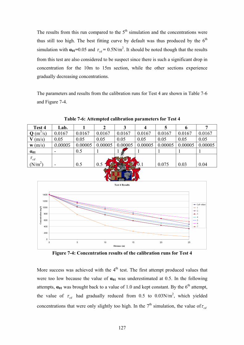
127

The results from this run compared to the 5th simulation and the concentrations were

thus still too high. The best fitting curve by default was thus produced by the 6th

simulation with α01=0.05 and cdτ = 0.5N/m2. It should be noted though that the results

from this test are also considered to be suspect since there is such a significant drop in

concentration for the 10m to 15m section, while the other sections experience

gradually decreasing concentrations.

The parameters and results from the calibration runs for Test 4 are shown in Table 7-6

and Figure 7-4.

Table 7-6: Attempted calibration parameters for Test 4

Test 4 Lab. 1 2 3 4 5 6 7 Q (m3/s) 0.0167 0.0167 0.0167 0.0167 0.0167 0.0167 0.0167 0.0167 V (m/s) 0.05 0.05 0.05 0.05 0.05 0.05 0.05 0.05 w (m/s) 0.00005 0.00005 0.00005 0.00005 0.00005 0.00005 0.00005 0.00005α01 - 0.5 1 1 1 1 1 1

cdτ (N/m2) - 0.5 0.5 0.4 0.1 0.075 0.03 0.04

Test 4 Results

0

200

400

600

800

1000

1200

1400

0 5 10 15 20 25

Distance (m)

Con

cent

ratio

n (m

g/l)

Lab values1234567

Figure 7-4: Concentration results of the calibration runs for Test 4

More success was achieved with the 4th test. The first attempt produced values that

were too low because the value of α01 was underestimated at 0.5. In the following

attempts, α01 was brought back to a value of 1.0 and kept constant. By the 6th attempt,

the value of cdτ had gradually reduced from 0.5 to 0.03N/m2, which yielded

concentrations that were only slightly too high. In the 7th simulation, the value of cdτ

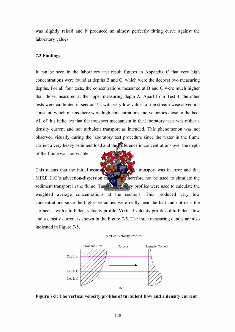
128

was slightly raised and it produced an almost perfectly fitting curve against the

laboratory values.

7.3 Findings

It can be seen in the laboratory test result figures in Appendix C that very high

concentrations were found at depths B and C, which were the deepest two measuring

depths. For all four tests, the concentrations measured at B and C were much higher

than those measured at the upper measuring depth A. Apart from Test 4, the other

tests were calibrated in section 7.2 with very low values of the stream wise advection

constant, which means there were high concentrations and velocities close to the bed.

All of this indicates that the transport mechanism in the laboratory tests was rather a

density current and not turbulent transport as intended. This phenomenon was not

observed visually during the laboratory test procedure since the water in the flume

carried a very heavy sediment load and the difference in concentrations over the depth

of the flume was not visible.

This means that the initial assumption of turbulent transport was in error and that

MIKE 21C’s advection-dispersion model can therefore not be used to simulate the

sediment transport in the flume. Turbulent velocity profiles were used to calculate the

weighted average concentrations at the sections. This produced very low

concentrations since the higher velocities were really near the bed and not near the

surface as with a turbulent velocity profile. Vertical velocity profiles of turbulent flow

and a density current is shown in the Figure 7-5. The three measuring depths are also

indicated in Figure 7-5.

Figure 7-5: The vertical velocity profiles of turbulent flow and a density current

129

The laboratory tests therefore produced averaged concentrations that were far too low

and these results were therefore deemed unreliable.

130

8. LONG TERM NUMERICAL STUDIES OF SEDIMENTATION

8.1 Background

In this chapter, MIKE 21C is used to model the transport of fine sediment for three

case-studies; Welbedacht Reservoir, Vaal Reservoir and Winam Gulf in Lake

Victoria. All of these three bodies of water experience silting of cohesive sediments

from their main tributaries. The three are, however, very different in size, catchment

area, annual runoff and sediment load. Welbedacht Reservoir is a narrow river

channel that experiences extremely large sediment loads. Vaal Reservoir is considered

to be a very large, wide and shallow reservoir with relatively low inflowing sediment

loads. Vaal Reservoir has in the past experienced some heavy sediment loads during

flood events.

These two reservoirs are thus extreme cases. Successful modelling of both with MIKE

21C will establish this software package as a powerful tool that can be used for all

South African reservoir sedimentation studies.

The third case study is Winam Gulf, a massive body of water with a small channel

that connects it to the main lake. The gulf is deep and wide and the water velocities

are very low. The gulf experiences varying water levels and is modelled in the same

way as the reservoirs. Application of the software to this case study is discussed in

section 8.4.

8.2 Welbedacht Reservoir Model

Welbedacht Dam was completed in 1973 on the Caledon River, draining a high

sediment yield region. During the first three years of operation the reservoir had lost

36 million m3 of it’s original 114 million m3 storage capacity due to sedimentation.

Figure 8.2-1 shows the losses in storage capacity over the years. Figure 8.2-2 shows

the longitudinal profile of the reservoir bed determined by survey data. Also shown in

Figure 8.2-2 is the future equilibrium sedimentation level of the reservoir as

calculated by Rooseboom et al. (1986).

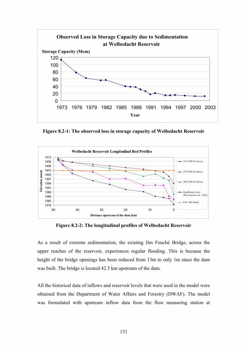
131

Figure 8.2-1: The observed loss in storage capacity of Welbedacht Reservoir

Welbedacht Reservoir Longitudinal Bed Profiles

137913821385138813911394139714001403140614091412

01020304050

Distance upstream of the dam (km)

Ele

vatio

n (m

asl)

1973 DWAF Survey

1976 DWAF Survey

2002 DWAF Survey

Equilibrium Level(Rooseboom et al., 1986)

FSL 1402.9masl

Figure 8.2-2: The longitudinal profiles of Welbedacht Reservoir

As a result of extreme sedimentation, the existing Jim Fouché Bridge, across the

upper reaches of the reservoir, experiences regular flooding. This is because the

height of the bridge openings has been reduced from 13m to only 1m since the dam

was built. The bridge is located 42.5 km upstream of the dam.

All the historical data of inflows and reservoir levels that were used in the model were

obtained from the Department of Water Affairs and Forestry (DWAF). The model

was formulated with upstream inflow data from the flow measuring station at

Observed Loss in Storage Capacity due to Sedimentation at Welbedacht Reservoir

0 20 40 60 80

100 120

1973 1976 1979 1982 1985 1988 1991 1994 1997 2000 2003Year

Storage Capacity (Mcm)

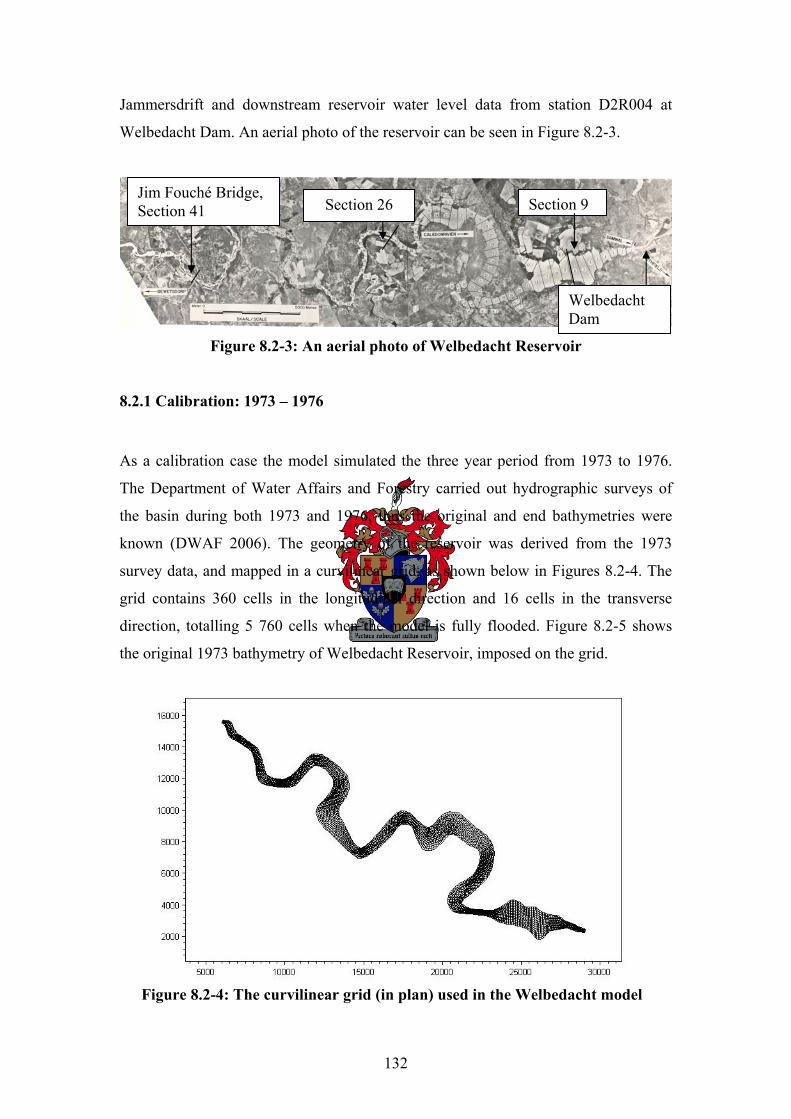
132

Jammersdrift and downstream reservoir water level data from station D2R004 at

Welbedacht Dam. An aerial photo of the reservoir can be seen in Figure 8.2-3.

Figure 8.2-3: An aerial photo of Welbedacht Reservoir

8.2.1 Calibration: 1973 – 1976

As a calibration case the model simulated the three year period from 1973 to 1976.

The Department of Water Affairs and Forestry carried out hydrographic surveys of

the basin during both 1973 and 1976, thus the original and end bathymetries were

known (DWAF 2006). The geometry of the reservoir was derived from the 1973

survey data, and mapped in a curvilinear grid, as shown below in Figures 8.2-4. The

grid contains 360 cells in the longitudinal direction and 16 cells in the transverse

direction, totalling 5 760 cells when the model is fully flooded. Figure 8.2-5 shows

the original 1973 bathymetry of Welbedacht Reservoir, imposed on the grid.

Figure 8.2-4: The curvilinear grid (in plan) used in the Welbedacht model

Welbedacht Dam

Jim Fouché Bridge, Section 41 Section 26 Section 9

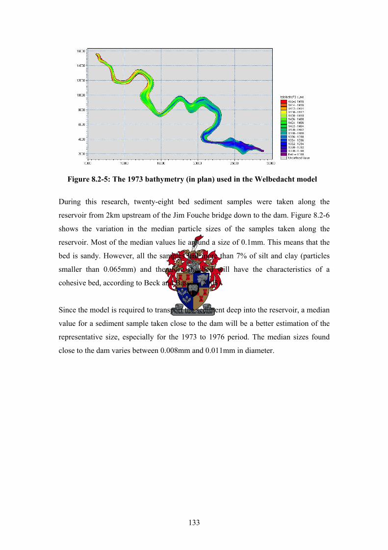
133

Figure 8.2-5: The 1973 bathymetry (in plan) used in the Welbedacht model

During this research, twenty-eight bed sediment samples were taken along the

reservoir from 2km upstream of the Jim Fouche bridge down to the dam. Figure 8.2-6

shows the variation in the median particle sizes of the samples taken along the

reservoir. Most of the median values lie around a size of 0.1mm. This means that the

bed is sandy. However, all the samples had more than 7% of silt and clay (particles

smaller than 0.065mm) and therefore the bed will have the characteristics of a

cohesive bed, according to Beck and Basson (2003).

Since the model is required to transport the sediment deep into the reservoir, a median

value for a sediment sample taken close to the dam will be a better estimation of the

representative size, especially for the 1973 to 1976 period. The median sizes found

close to the dam varies between 0.008mm and 0.011mm in diameter.

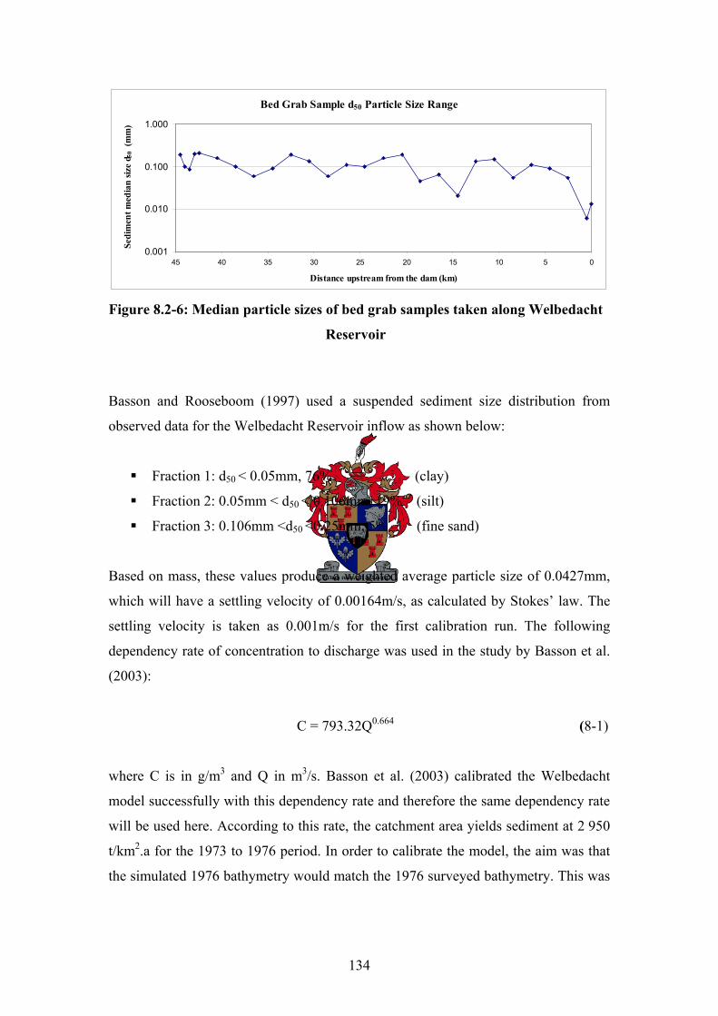
134

Bed Grab Sample d50 Particle Size Range

0.001

0.010

0.100

1.000

051015202530354045

Distance upstream from the dam (km)

Sedi

men

t med

ian

size

d 50

(mm

)

Figure 8.2-6: Median particle sizes of bed grab samples taken along Welbedacht

Reservoir

Basson and Rooseboom (1997) used a suspended sediment size distribution from

observed data for the Welbedacht Reservoir inflow as shown below:

Fraction 1: d50 < 0.05mm, 76% (clay)

Fraction 2: 0.05mm < d50 < 0.106mm, 19% (silt)

Fraction 3: 0.106mm <d50 <0.25mm, 5% (fine sand)

Based on mass, these values produce a weighted average particle size of 0.0427mm,

which will have a settling velocity of 0.00164m/s, as calculated by Stokes’ law. The

settling velocity is taken as 0.001m/s for the first calibration run. The following

dependency rate of concentration to discharge was used in the study by Basson et al.

(2003):

C = 793.32Q0.664 (8-1)

where C is in g/m3 and Q in m3/s. Basson et al. (2003) calibrated the Welbedacht

model successfully with this dependency rate and therefore the same dependency rate

will be used here. According to this rate, the catchment area yields sediment at 2 950

t/km2.a for the 1973 to 1976 period. In order to calibrate the model, the aim was that

the simulated 1976 bathymetry would match the 1976 surveyed bathymetry. This was

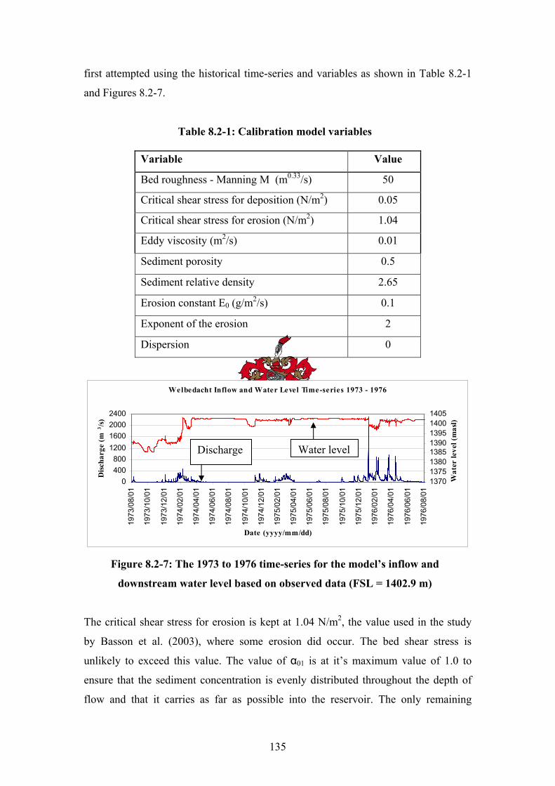
135

first attempted using the historical time-series and variables as shown in Table 8.2-1

and Figures 8.2-7.

Table 8.2-1: Calibration model variables

Variable Value

Bed roughness - Manning M (m0.33/s) 50

Critical shear stress for deposition (N/m2) 0.05

Critical shear stress for erosion (N/m2) 1.04

Eddy viscosity (m2/s) 0.01

Sediment porosity 0.5

Sediment relative density 2.65

Erosion constant E0 (g/m2/s) 0.1

Exponent of the erosion 2

Dispersion 0

Welbedacht Inflow and Water Level Time-series 1973 - 1976

0400800

1200160020002400

1973

/08/

01

1973

/10/

01

1973

/12/

01

1974

/02/

01

1974

/04/

01

1974

/06/

01

1974

/08/

01

1974

/10/

01

1974

/12/

01

1975

/02/

01

1975

/04/

01

1975

/06/

01

1975

/08/

01

1975

/10/

01

1975

/12/

01

1976

/02/

01

1976

/04/

01

1976

/06/

01

1976

/08/

01

Date (yyyy/mm/dd)

Disc

harg

e (m

3 /s)

13701375138013851390139514001405

Wat

er le

vel (

mas

l)

Figure 8.2-7: The 1973 to 1976 time-series for the model’s inflow and

downstream water level based on observed data (FSL = 1402.9 m)

The critical shear stress for erosion is kept at 1.04 N/m2, the value used in the study

by Basson et al. (2003), where some erosion did occur. The bed shear stress is

unlikely to exceed this value. The value of α01 is at it’s maximum value of 1.0 to

ensure that the sediment concentration is evenly distributed throughout the depth of

flow and that it carries as far as possible into the reservoir. The only remaining

Water levelDischarge

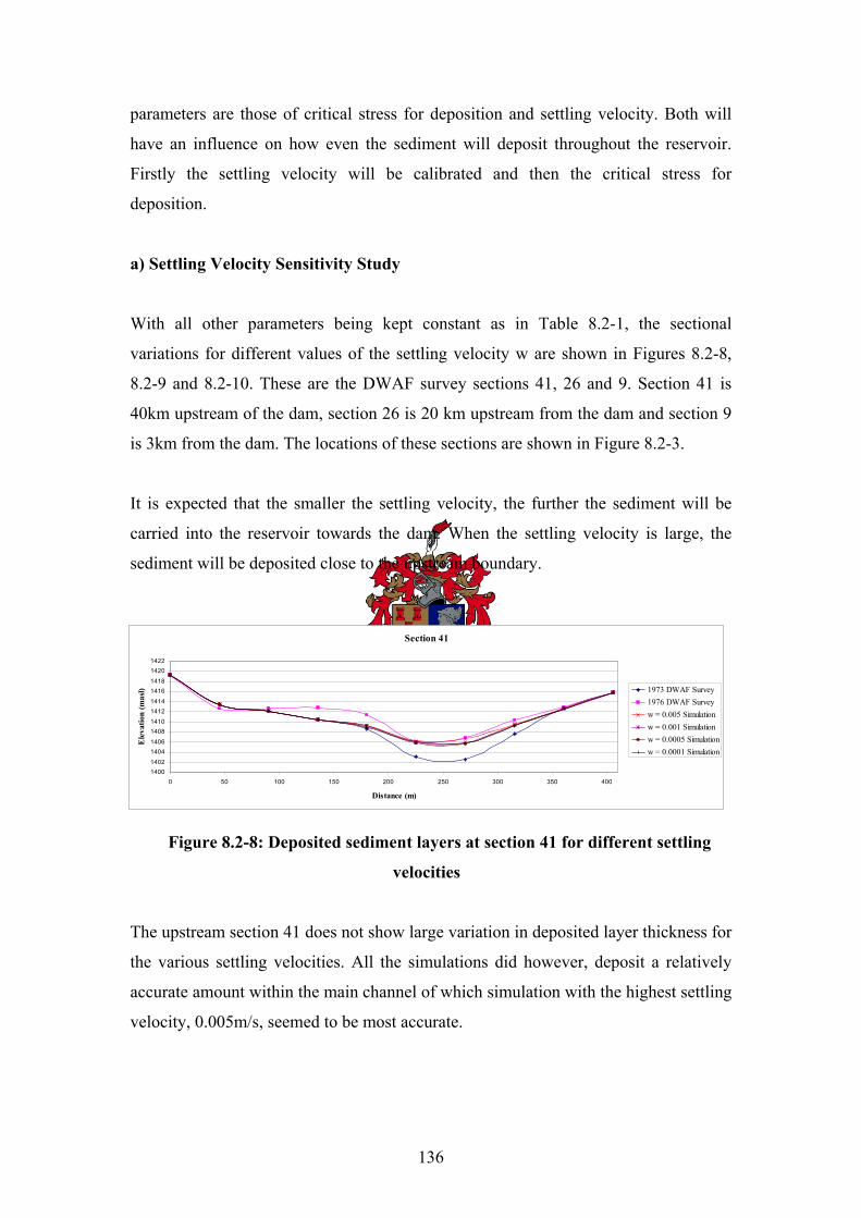
136

parameters are those of critical stress for deposition and settling velocity. Both will

have an influence on how even the sediment will deposit throughout the reservoir.

Firstly the settling velocity will be calibrated and then the critical stress for

deposition.

a) Settling Velocity Sensitivity Study

With all other parameters being kept constant as in Table 8.2-1, the sectional

variations for different values of the settling velocity w are shown in Figures 8.2-8,

8.2-9 and 8.2-10. These are the DWAF survey sections 41, 26 and 9. Section 41 is

40km upstream of the dam, section 26 is 20 km upstream from the dam and section 9

is 3km from the dam. The locations of these sections are shown in Figure 8.2-3.

It is expected that the smaller the settling velocity, the further the sediment will be

carried into the reservoir towards the dam. When the settling velocity is large, the

sediment will be deposited close to the upstream boundary.

Section 41

14001402

14041406

14081410141214141416141814201422

0 50 100 150 200 250 300 350 400

Distance (m)

Ele

vatio

n (m

asl) 1973 DWAF Survey

1976 DWAF Surveyw = 0.005 Simulationw = 0.001 Simulationw = 0.0005 Simulationw = 0.0001 Simulation

Figure 8.2-8: Deposited sediment layers at section 41 for different settling

velocities

The upstream section 41 does not show large variation in deposited layer thickness for

the various settling velocities. All the simulations did however, deposit a relatively

accurate amount within the main channel of which simulation with the highest settling

velocity, 0.005m/s, seemed to be most accurate.

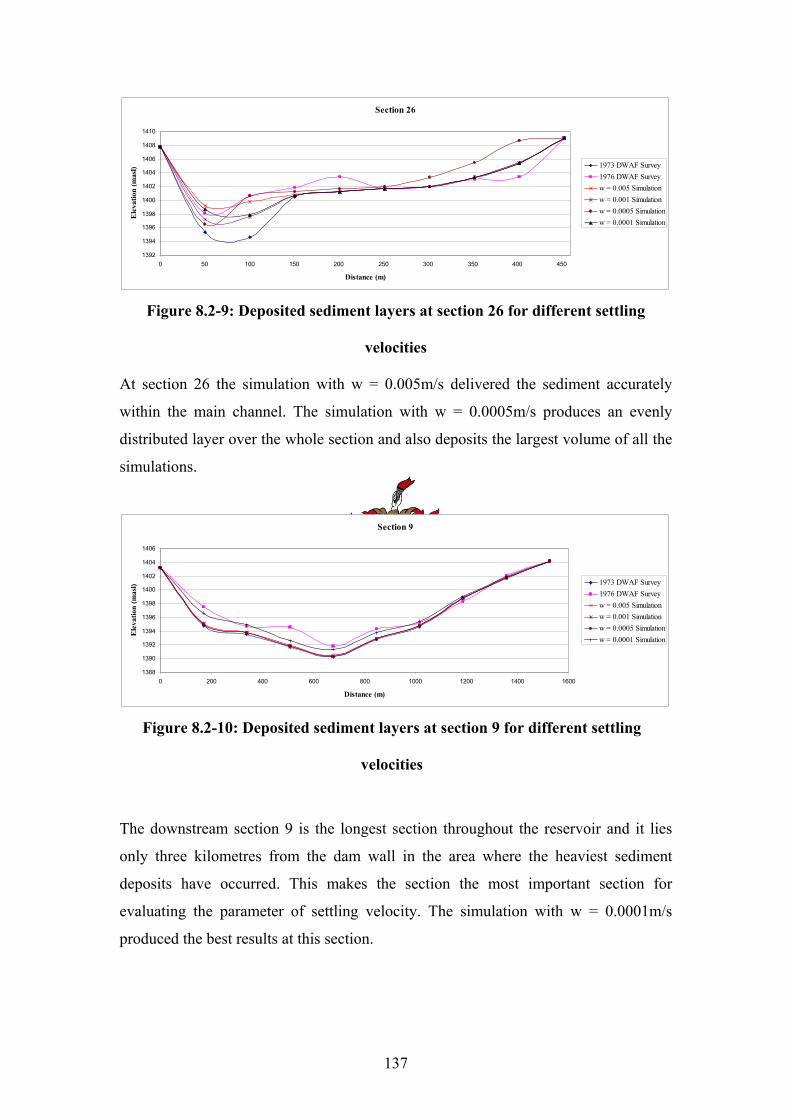
137

Section 26

1392

1394

1396

1398

1400

1402

1404

1406

1408

1410

0 50 100 150 200 250 300 350 400 450

Distance (m)

Ele

vatio

n (m

asl) 1973 DWAF Survey

1976 DWAF Surveyw = 0.005 Simulationw = 0.001 Simulationw = 0.0005 Simulationw = 0.0001 Simulation

Figure 8.2-9: Deposited sediment layers at section 26 for different settling

velocities

At section 26 the simulation with w = 0.005m/s delivered the sediment accurately

within the main channel. The simulation with w = 0.0005m/s produces an evenly

distributed layer over the whole section and also deposits the largest volume of all the

simulations.

Section 9

1388

1390

1392

1394

1396

1398

1400

1402

1404

1406

0 200 400 600 800 1000 1200 1400 1600

Distance (m)

Ele

vatio

n (m

asl) 1973 DWAF Survey

1976 DWAF Surveyw = 0.005 Simulationw = 0.001 Simulationw = 0.0005 Simulationw = 0.0001 Simulation

Figure 8.2-10: Deposited sediment layers at section 9 for different settling

velocities

The downstream section 9 is the longest section throughout the reservoir and it lies

only three kilometres from the dam wall in the area where the heaviest sediment

deposits have occurred. This makes the section the most important section for

evaluating the parameter of settling velocity. The simulation with w = 0.0001m/s

produced the best results at this section.

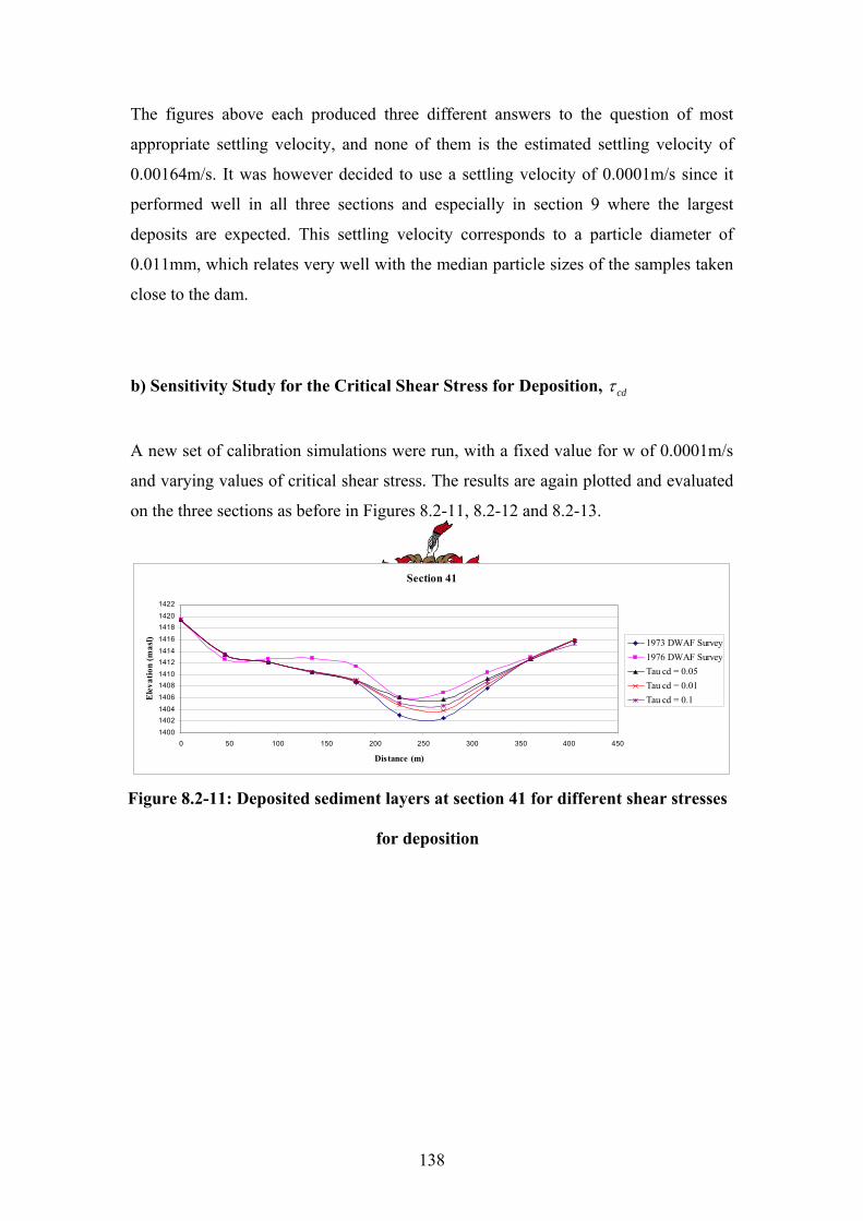
138

The figures above each produced three different answers to the question of most

appropriate settling velocity, and none of them is the estimated settling velocity of

0.00164m/s. It was however decided to use a settling velocity of 0.0001m/s since it

performed well in all three sections and especially in section 9 where the largest

deposits are expected. This settling velocity corresponds to a particle diameter of

0.011mm, which relates very well with the median particle sizes of the samples taken

close to the dam.

b) Sensitivity Study for the Critical Shear Stress for Deposition, cdτ

A new set of calibration simulations were run, with a fixed value for w of 0.0001m/s

and varying values of critical shear stress. The results are again plotted and evaluated

on the three sections as before in Figures 8.2-11, 8.2-12 and 8.2-13.

Section 41

1400

14021404

140614081410141214141416

14181420

1422

0 50 100 150 200 250 300 350 400 450

Distance (m)

Ele

vatio

n (m

asl) 1973 DWAF Survey

1976 DWAF SurveyTau cd = 0.05Tau cd = 0.01Tau cd = 0.1

Figure 8.2-11: Deposited sediment layers at section 41 for different shear stresses

for deposition

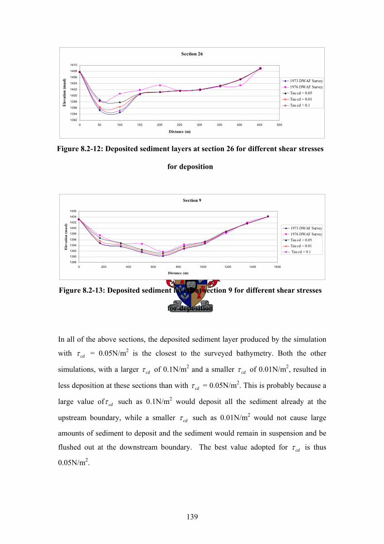
139

Section 26

1392

1394

1396

1398

1400

1402

1404

1406

1408

1410

0 50 100 150 200 250 300 350 400 450 500

Distance (m)

Ele

vatio

n (m

asl) 1973 DWAF Survey

1976 DWAF SurveyTau cd = 0.05Tau cd = 0.01Tau cd = 0.1

Figure 8.2-12: Deposited sediment layers at section 26 for different shear stresses

for deposition

Section 9

1388

1390

1392

1394

1396

1398

1400

1402

1404

1406

0 200 400 600 800 1000 1200 1400 1600

Distance (m)

Ele

vatio

n (m

asl)

1973 DWAF Survey1976 DWAF SurveyTau cd = 0.05Tau cd = 0.01 Tau cd = 0.1

Figure 8.2-13: Deposited sediment layers at section 9 for different shear stresses

for deposition

In all of the above sections, the deposited sediment layer produced by the simulation

with cdτ = 0.05N/m2 is the closest to the surveyed bathymetry. Both the other

simulations, with a larger cdτ of 0.1N/m2 and a smaller cdτ of 0.01N/m2, resulted in

less deposition at these sections than with cdτ = 0.05N/m2. This is probably because a

large value of cdτ such as 0.1N/m2 would deposit all the sediment already at the

upstream boundary, while a smaller cdτ such as 0.01N/m2 would not cause large

amounts of sediment to deposit and the sediment would remain in suspension and be

flushed out at the downstream boundary. The best value adopted for cdτ is thus

0.05N/m2.

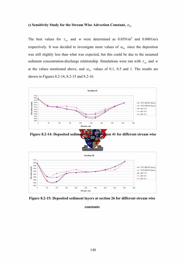
140

c) Sensitivity Study for the Stream Wise Advection Constant, 01α

The best values for cdτ and w were determined as 0.05N/m2 and 0.0001m/s

respectively. It was decided to investigate more values of 01α since the deposition

was still slightly less than what was expected, but this could be due to the assumed

sediment concentration-discharge relationship. Simulations were run with cdτ and w

at the values mentioned above, and 01α values of 0.1, 0.5 and 1. The results are

shown in Figures 8.2-14, 8.2-15 and 8.2-16.

Section 41

14001402

14041406

14081410

14121414

14161418

14201422

0 50 100 150 200 250 300 350 400 450

Distance (m)

Ele

vatio

n (m

asl) 1973 DWAF Survey

1976 DWAF Surveyα01=1.0α01=0.5α01=0.1

Figure 8.2-14: Deposited sediment layers at section 41 for different stream wise

constants

Section 26

1392

1394

1396

1398

1400

1402

1404

1406

1408

1410

0 50 100 150 200 250 300 350 400 450 500

Distance (m)

Ele

vatio

n (m

asl) 1973 DWAF Survey

1976 DWAF Surveyα01=1.0α01=0.5α01=0.1

Figure 8.2-15: Deposited sediment layers at section 26 for different stream wise

constants

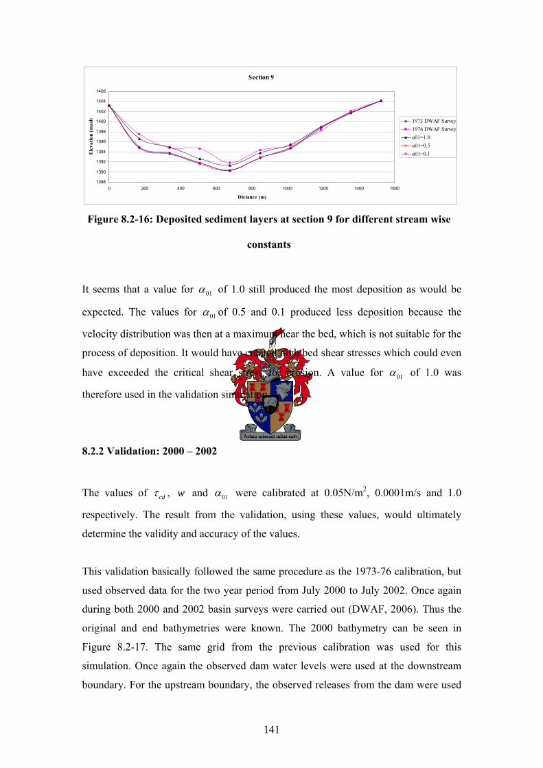
141

Section 9

1388

1390

1392

1394

1396

1398

1400

1402

1404

1406

0 200 400 600 800 1000 1200 1400 1600

Distance (m)

Ele

vatio

n (m

asl) 1973 DWAF Survey

1976 DWAF Surveyα01=1.0α01=0.5α01=0.1

Figure 8.2-16: Deposited sediment layers at section 9 for different stream wise

constants

It seems that a value for 01α of 1.0 still produced the most deposition as would be

expected. The values for 01α of 0.5 and 0.1 produced less deposition because the

velocity distribution was then at a maximum near the bed, which is not suitable for the

process of deposition. It would have created high bed shear stresses which could even

have exceeded the critical shear stress for erosion. A value for 01α of 1.0 was

therefore used in the validation simulation.

8.2.2 Validation: 2000 – 2002

The values of cdτ , w and 01α were calibrated at 0.05N/m2, 0.0001m/s and 1.0

respectively. The result from the validation, using these values, would ultimately

determine the validity and accuracy of the values.

This validation basically followed the same procedure as the 1973-76 calibration, but

used observed data for the two year period from July 2000 to July 2002. Once again

during both 2000 and 2002 basin surveys were carried out (DWAF, 2006). Thus the

original and end bathymetries were known. The 2000 bathymetry can be seen in

Figure 8.2-17. The same grid from the previous calibration was used for this

simulation. Once again the observed dam water levels were used at the downstream

boundary. For the upstream boundary, the observed releases from the dam were used

142

since the upstream Jammersdrift gauging station was no longer operational during this

period.

Figure 8.2-17: The 2000 survey bathymetry (in plan) used for the validation

Due to the high silt content the cohesive modelling approach adopted for the 1973-

1976 simulation was again used for the 2000 to 2002 period. No upstream sediment

concentrations have been monitored since 1976, and the original concentration-

discharge relationship for 1973 to 1976 was again used for the sediment yield. The

variables and historical time-series are shown in Table 8.2-2 and Figure 8.2-18:

Table 8.2-2: Validation model variables

Variable Value

Bed roughness - Manning M (m0.33/s) 50

Critical shear stress for deposition (N/m2) 0.05

Critical shear stress for erosion (N/m2) 1.04

Eddy viscosity (m2/s) 0.01

Fall velocity (m/s) 0.0001

Stream wise constant α01 1.0

Sediment porosity 0.5

Sediment relative density 2.65

Erosion constant E0 (g/m2/s) 0.1

Exponent of the erosion 2

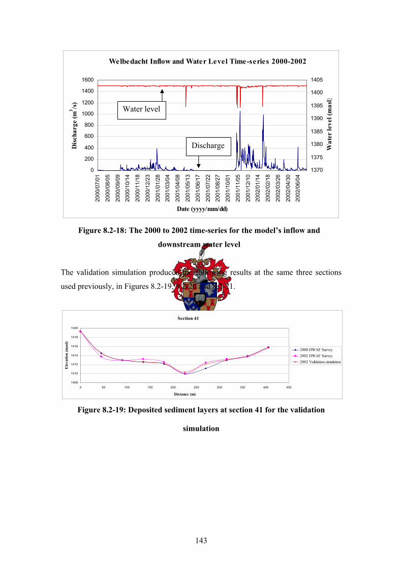
143

Welbedacht Inflow and Water Level Time-series 2000-2002

0

200

400

600

800

1000

1200

1400

1600

2000

/07/

01

2000

/08/

05

2000

/09/

09

2000

/10/

14

2000

/11/

18

2000

/12/

23

2001

/01/

28

2001

/03/

04

2001

/04/

08

2001

/05/

13

2001

/06/

17

2001

/07/

22

2001

/08/

27

2001

/10/

01

2001

/11/

05

2001

/12/

10

2002

/01/

14

2002

/02/

18

2002

/03/

26

2002

/04/

30

2002

/06/

04

Date (yyyy/mm/dd)

Dis

char

ge (m

3 /s)

1370

1375

1380

1385

1390

1395

1400

1405

Wat

er le

vel (

mas

l)

Figure 8.2-18: The 2000 to 2002 time-series for the model’s inflow and

downstream water level

The validation simulation produced the following results at the same three sections

used previously, in Figures 8.2-19, 8.2-20 and 8.2-21.

Section 41

1408

1410

1412

1414

1416

1418

1420

0 50 100 150 200 250 300 350 400 450

Distance (m)

Ele

vatio

n (m

asl)

2000 DWAF Survey2002 DWAF Survey2002 Validation simulation

Figure 8.2-19: Deposited sediment layers at section 41 for the validation

simulation

Water level

Discharge

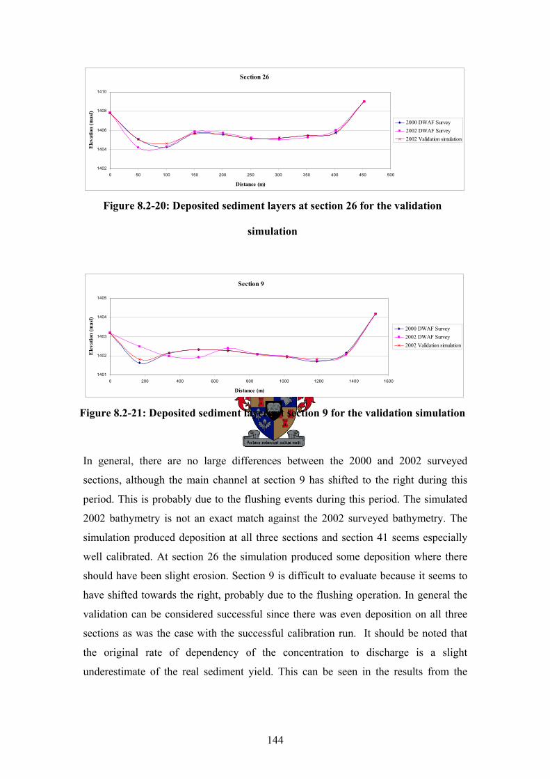
144

Section 26

1402

1404

1406

1408

1410

0 50 100 150 200 250 300 350 400 450 500

Distance (m)

Ele

vatio

n (m

asl)

2000 DWAF Survey2002 DWAF Survey2002 Validation simulation

Figure 8.2-20: Deposited sediment layers at section 26 for the validation

simulation

Section 9

1401

1402

1403

1404

1405

0 200 400 600 800 1000 1200 1400 1600

Distance (m)

Ele

vatio

n (m

asl)

2000 DWAF Survey2002 DWAF Survey2002 Validation simulation

Figure 8.2-21: Deposited sediment layers at section 9 for the validation simulation

In general, there are no large differences between the 2000 and 2002 surveyed

sections, although the main channel at section 9 has shifted to the right during this

period. This is probably due to the flushing events during this period. The simulated

2002 bathymetry is not an exact match against the 2002 surveyed bathymetry. The

simulation produced deposition at all three sections and section 41 seems especially

well calibrated. At section 26 the simulation produced some deposition where there

should have been slight erosion. Section 9 is difficult to evaluate because it seems to

have shifted towards the right, probably due to the flushing operation. In general the

validation can be considered successful since there was even deposition on all three

sections as was the case with the successful calibration run. It should be noted that

the original rate of dependency of the concentration to discharge is a slight

underestimate of the real sediment yield. This can be seen in the results from the

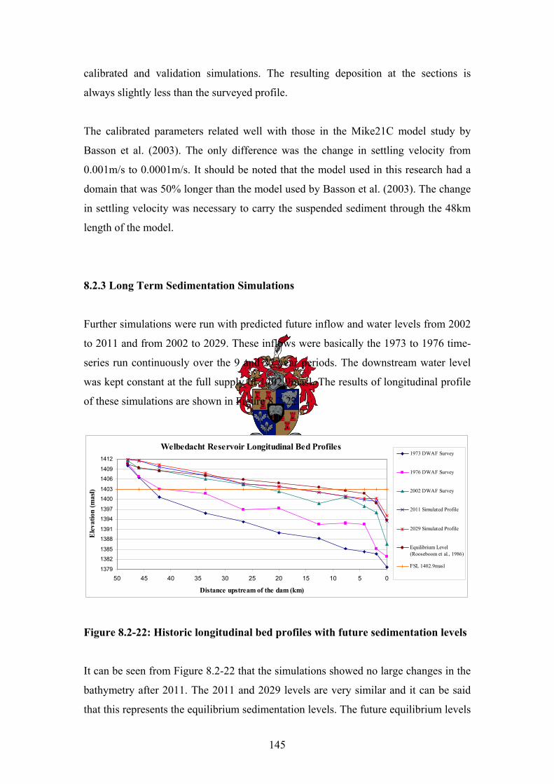
145

calibrated and validation simulations. The resulting deposition at the sections is

always slightly less than the surveyed profile.

The calibrated parameters related well with those in the Mike21C model study by

Basson et al. (2003). The only difference was the change in settling velocity from

0.001m/s to 0.0001m/s. It should be noted that the model used in this research had a

domain that was 50% longer than the model used by Basson et al. (2003). The change

in settling velocity was necessary to carry the suspended sediment through the 48km

length of the model.

8.2.3 Long Term Sedimentation Simulations

Further simulations were run with predicted future inflow and water levels from 2002

to 2011 and from 2002 to 2029. These inflows were basically the 1973 to 1976 time-

series run continuously over the 9 and 27 year periods. The downstream water level

was kept constant at the full supply of 1402.9masl. The results of longitudinal profile

of these simulations are shown in Figure 8.2-22.

Welbedacht Reservoir Longitudinal Bed Profiles

1379

1382

1385

1388

1391

1394

1397

1400

1403

1406

1409

1412

05101520253035404550

Distance upstream of the dam (km)

Ele

vatio

n (m

asl)

1973 DWAF Survey

1976 DWAF Survey

2002 DWAF Survey

2011 Simulated Profile

2029 Simulated Profile

Equilibrium Level(Rooseboom et al., 1986)

FSL 1402.9masl

Figure 8.2-22: Historic longitudinal bed profiles with future sedimentation levels

It can be seen from Figure 8.2-22 that the simulations showed no large changes in the

bathymetry after 2011. The 2011 and 2029 levels are very similar and it can be said

that this represents the equilibrium sedimentation levels. The future equilibrium levels

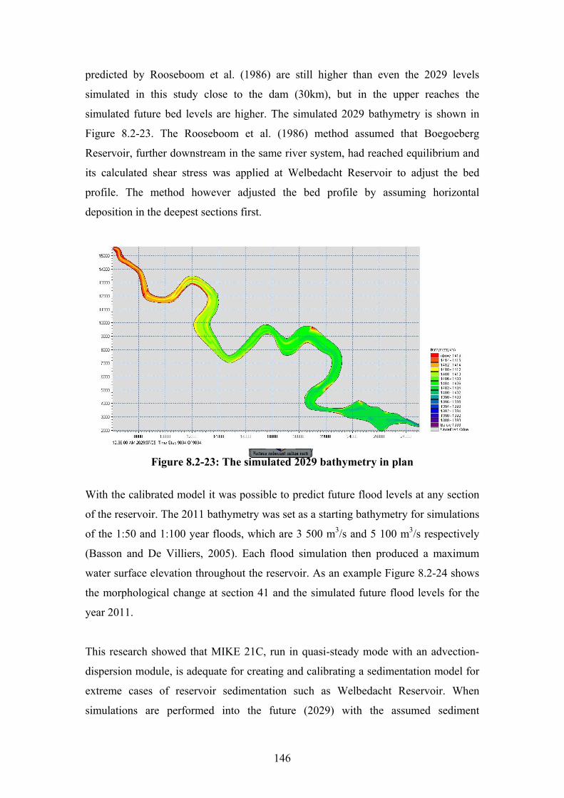
146

predicted by Rooseboom et al. (1986) are still higher than even the 2029 levels

simulated in this study close to the dam (30km), but in the upper reaches the

simulated future bed levels are higher. The simulated 2029 bathymetry is shown in

Figure 8.2-23. The Rooseboom et al. (1986) method assumed that Boegoeberg

Reservoir, further downstream in the same river system, had reached equilibrium and

its calculated shear stress was applied at Welbedacht Reservoir to adjust the bed

profile. The method however adjusted the bed profile by assuming horizontal

deposition in the deepest sections first.

Figure 8.2-23: The simulated 2029 bathymetry in plan

With the calibrated model it was possible to predict future flood levels at any section

of the reservoir. The 2011 bathymetry was set as a starting bathymetry for simulations

of the 1:50 and 1:100 year floods, which are 3 500 m3/s and 5 100 m3/s respectively

(Basson and De Villiers, 2005). Each flood simulation then produced a maximum

water surface elevation throughout the reservoir. As an example Figure 8.2-24 shows

the morphological change at section 41 and the simulated future flood levels for the

year 2011.

This research showed that MIKE 21C, run in quasi-steady mode with an advection-

dispersion module, is adequate for creating and calibrating a sedimentation model for

extreme cases of reservoir sedimentation such as Welbedacht Reservoir. When

simulations are performed into the future (2029) with the assumed sediment

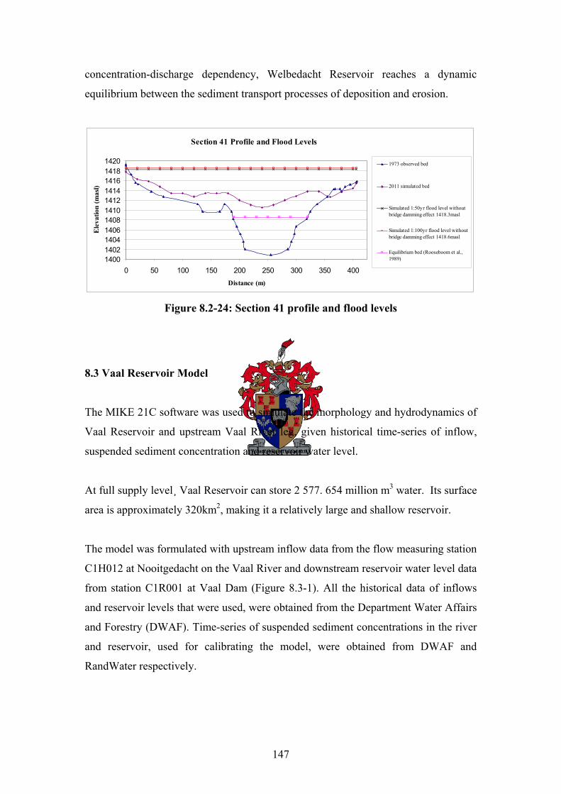
147

concentration-discharge dependency, Welbedacht Reservoir reaches a dynamic

equilibrium between the sediment transport processes of deposition and erosion.

Section 41 Profile and Flood Levels

14001402140414061408141014121414141614181420

0 50 100 150 200 250 300 350 400

Distance (m)

Ele

vatio

n (m

asl)

1973 observed bed

2011 simulated bed

Simulated 1:50yr flood level withoutbridge damming effect 1418.3masl

Simulated 1:100yr flood level withoutbridge damming effect 1418.6masl

Equilibrium bed (Rooseboom et al.,1989)

Figure 8.2-24: Section 41 profile and flood levels

8.3 Vaal Reservoir Model

The MIKE 21C software was used to simulate the morphology and hydrodynamics of

Vaal Reservoir and upstream Vaal River leg, given historical time-series of inflow,

suspended sediment concentration and reservoir water level.

At full supply level¸ Vaal Reservoir can store 2 577. 654 million m3 water. Its surface

area is approximately 320km2, making it a relatively large and shallow reservoir.

The model was formulated with upstream inflow data from the flow measuring station

C1H012 at Nooitgedacht on the Vaal River and downstream reservoir water level data

from station C1R001 at Vaal Dam (Figure 8.3-1). All the historical data of inflows

and reservoir levels that were used, were obtained from the Department Water Affairs

and Forestry (DWAF). Time-series of suspended sediment concentrations in the river

and reservoir, used for calibrating the model, were obtained from DWAF and

RandWater respectively.

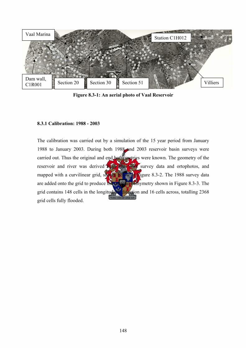
148

Figure 8.3-1: An aerial photo of Vaal Reservoir

8.3.1 Calibration: 1988 - 2003

The calibration was carried out by a simulation of the 15 year period from January

1988 to January 2003. During both 1988 and 2003 reservoir basin surveys were

carried out. Thus the original and end bathymetries were known. The geometry of the

reservoir and river was derived from the 1988 survey data and ortophotos, and

mapped with a curvilinear grid, shown below in Figure 8.3-2. The 1988 survey data

are added onto the grid to produce the original bathymetry shown in Figure 8.3-3. The

grid contains 148 cells in the longitudinal direction and 16 cells across, totalling 2368

grid cells fully flooded.

Villiers Dam wall, C1R001

Vaal Marina Station C1H012

Section 20 Section 30 Section 51

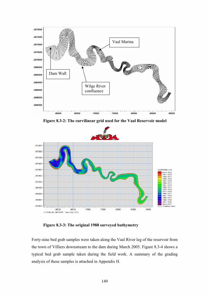
149

Figure 8.3-2: The curvilinear grid used for the Vaal Reservoir model

Figure 8.3-3: The original 1988 surveyed bathymetry

Forty-nine bed grab samples were taken along the Vaal River leg of the reservoir from

the town of Villiers downstream to the dam during March 2005. Figure 8.3-4 shows a

typical bed grab sample taken during the field work. A summary of the grading

analysis of these samples is attached in Appendix H.

Dam Wall

Wilge River confluence

Vaal Marina

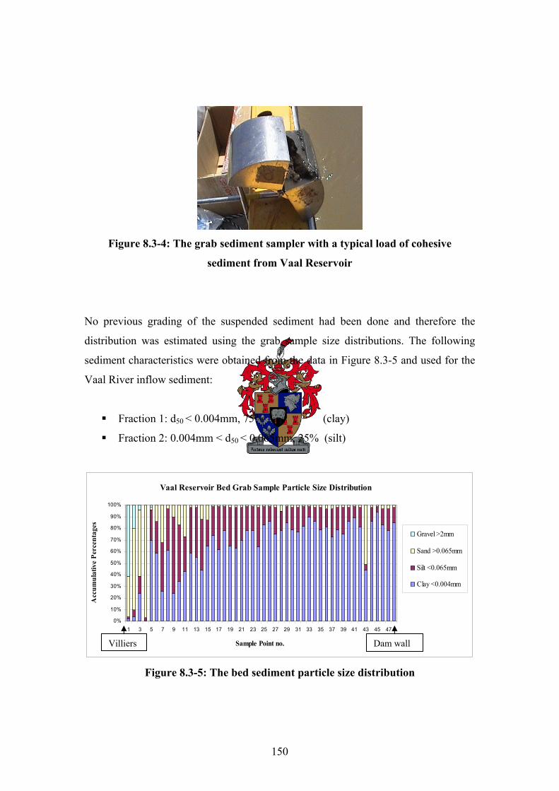
150

Figure 8.3-4: The grab sediment sampler with a typical load of cohesive

sediment from Vaal Reservoir

No previous grading of the suspended sediment had been done and therefore the

distribution was estimated using the grab sample size distributions. The following

sediment characteristics were obtained from the data in Figure 8.3-5 and used for the

Vaal River inflow sediment:

Fraction 1: d50 < 0.004mm, 75% (clay)

Fraction 2: 0.004mm < d50 < 0.065mm, 25% (silt)

Vaal Reservoir Bed Grab Sample Particle Size Distribution

0%

10%

20%

30%

40%

50%

60%

70%

80%

90%

100%

1 3 5 7 9 11 13 15 17 19 21 23 25 27 29 31 33 35 37 39 41 43 45 47

Sample Point no.

Acc

umul

ativ

e Pe

rcen

tage

s

Gravel >2mm

Sand >0.065mm

Silt <0.065mm

Clay <0.004mm

Figure 8.3-5: The bed sediment particle size distribution

Dam wall Villiers

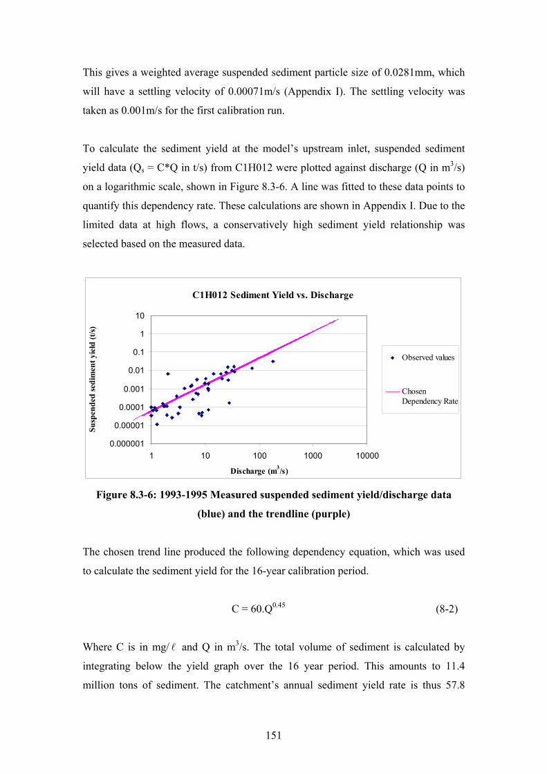
151

This gives a weighted average suspended sediment particle size of 0.0281mm, which

will have a settling velocity of 0.00071m/s (Appendix I). The settling velocity was

taken as 0.001m/s for the first calibration run.

To calculate the sediment yield at the model’s upstream inlet, suspended sediment

yield data (Qs = C*Q in t/s) from C1H012 were plotted against discharge (Q in m3/s)

on a logarithmic scale, shown in Figure 8.3-6. A line was fitted to these data points to

quantify this dependency rate. These calculations are shown in Appendix I. Due to the

limited data at high flows, a conservatively high sediment yield relationship was

selected based on the measured data.

C1H012 Sediment Yield vs. Discharge

0.000001

0.00001

0.0001

0.001

0.01

0.1

1

10

1 10 100 1000 10000

Discharge (m3/s)

Susp

ende

d se

dim

ent y

ield

(t/s)

Observed values

ChosenDependency Rate

Figure 8.3-6: 1993-1995 Measured suspended sediment yield/discharge data

(blue) and the trendline (purple)

The chosen trend line produced the following dependency equation, which was used

to calculate the sediment yield for the 16-year calibration period.

C = 60.Q0.45 (8-2)

Where C is in mg/ l and Q in m3/s. The total volume of sediment is calculated by

integrating below the yield graph over the 16 year period. This amounts to 11.4

million tons of sediment. The catchment’s annual sediment yield rate is thus 57.8

152

ton/km2.a considering an effective catchment area downstream of Grootdraai Dam of

12 276 km2. (Appendix I). This value is a lot less than the rate of 193 ton/km2.a

predicted by Rooseboom and Maas (1974) and the maximum observed regional yield

of 150 t/km2.a (Rooseboom et al., 1992).

To calibrate the model, the aim was that the simulated 2003 bathymetry matched the

2003 surveyed bathymetry. Also the output time series data of suspended sediment

concentrations had to compare with the data from RandWater.

This was attempted using the following historical time series and variables as shown

in Table 8.2-1 and Figures 8.2-7 and 8.2-8. All the measured values of discharge

lower than 10m3/s, were taken as 10m3/s. This made it easier for the program to run

the simulation, as lower flows can make the calculations unstable. This time series

contained the 1:100 year flood of February 1996, for which the model’s side

boundaries had to be lifted by 10m so that the extreme flow would not overtop the

model’s sides and cause the simulation to become unstable. Very little or no erosion is

expected to take place and therefore the critical shear stress for erosion is kept

sufficiently high (1.04N/m2) as was calibrated previously for Welbedacht Reservoir

by DHI (2003). The bed shear stress is unlikely to exceed this value.

From the Welbedacht study it was clear that the value of α01 can not be any less than

1.0 for reservoir applications. A value for α01 of 1.0 was again used here. The other

parameters were as shown in Table 8.3-1. The model’s inflow and water level time-

series are shown in Figure 8.3-7.

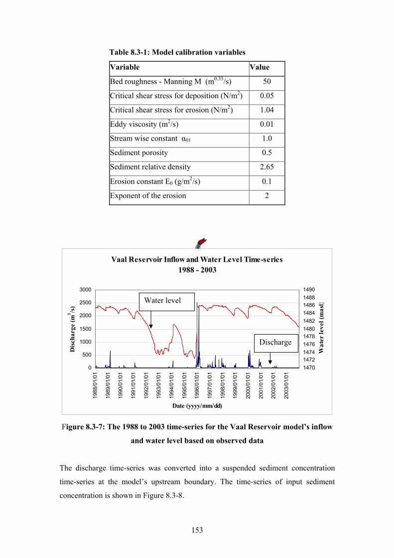
153

Table 8.3-1: Model calibration variables

Variable Value

Bed roughness - Manning M (m0.33/s) 50

Critical shear stress for deposition (N/m2) 0.05

Critical shear stress for erosion (N/m2) 1.04

Eddy viscosity (m2/s) 0.01

Stream wise constant α01 1.0

Sediment porosity 0.5

Sediment relative density 2.65

Erosion constant E0 (g/m2/s) 0.1

Exponent of the erosion 2

Vaal Reservoir Inflow and Water Level Time-series 1988 - 2003

0

500

1000

1500

2000

2500

3000

1988

/01/

01

1989

/01/

01

1990

/01/

01

1991

/01/

01

1992

/01/

01

1993

/01/

01

1994

/01/

01

1995

/01/

01

1996

/01/

01

1997

/01/

01

1998

/01/

01

1999

/01/

01

2000

/01/

01

2001

/01/

01

2002

/01/

01

2003

/01/

01

Date (yyyy/mm/dd)

Dis

char

ge (m

3 /s)

14701472147414761478148014821484148614881490

Wat

er le

vel (

mas

l)

Figure 8.3-7: The 1988 to 2003 time-series for the Vaal Reservoir model’s inflow

and water level based on observed data

The discharge time-series was converted into a suspended sediment concentration

time-series at the model’s upstream boundary. The time-series of input sediment

concentration is shown in Figure 8.3-8.

Water level

Discharge

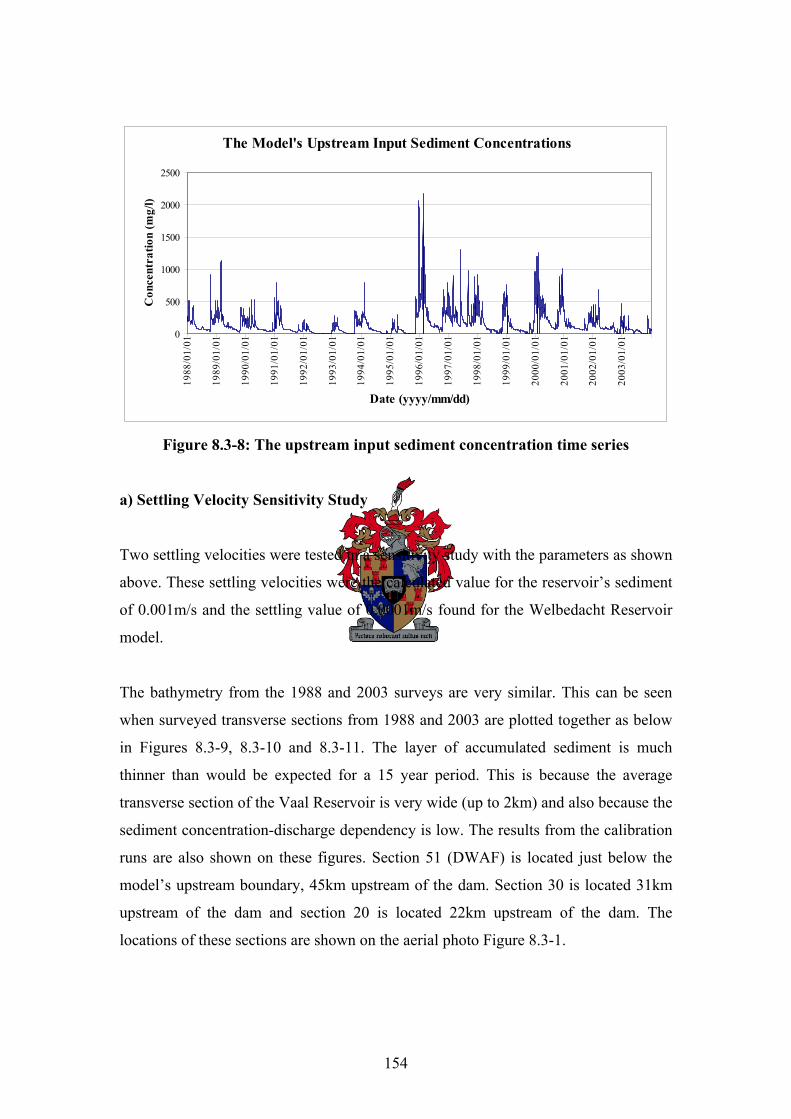
154

The Model's Upstream Input Sediment Concentrations

0

500

1000

1500

2000

250019

88/0

1/01

1989

/01/

01

1990

/01/

01

1991

/01/

01

1992

/01/

01

1993

/01/

01

1994

/01/

01

1995

/01/

01

1996

/01/

01

1997

/01/

01

1998

/01/

01

1999

/01/

01

2000

/01/

01

2001

/01/

01

2002

/01/

01

2003

/01/

01

Date (yyyy/mm/dd)

Con

cent

ratio

n (m

g/l)

Figure 8.3-8: The upstream input sediment concentration time series

a) Settling Velocity Sensitivity Study

Two settling velocities were tested in a sensitivity study with the parameters as shown

above. These settling velocities were the calculated value for the reservoir’s sediment

of 0.001m/s and the settling value of 0.0001m/s found for the Welbedacht Reservoir

model.

The bathymetry from the 1988 and 2003 surveys are very similar. This can be seen

when surveyed transverse sections from 1988 and 2003 are plotted together as below

in Figures 8.3-9, 8.3-10 and 8.3-11. The layer of accumulated sediment is much

thinner than would be expected for a 15 year period. This is because the average

transverse section of the Vaal Reservoir is very wide (up to 2km) and also because the

sediment concentration-discharge dependency is low. The results from the calibration

runs are also shown on these figures. Section 51 (DWAF) is located just below the

model’s upstream boundary, 45km upstream of the dam. Section 30 is located 31km

upstream of the dam and section 20 is located 22km upstream of the dam. The

locations of these sections are shown on the aerial photo Figure 8.3-1.

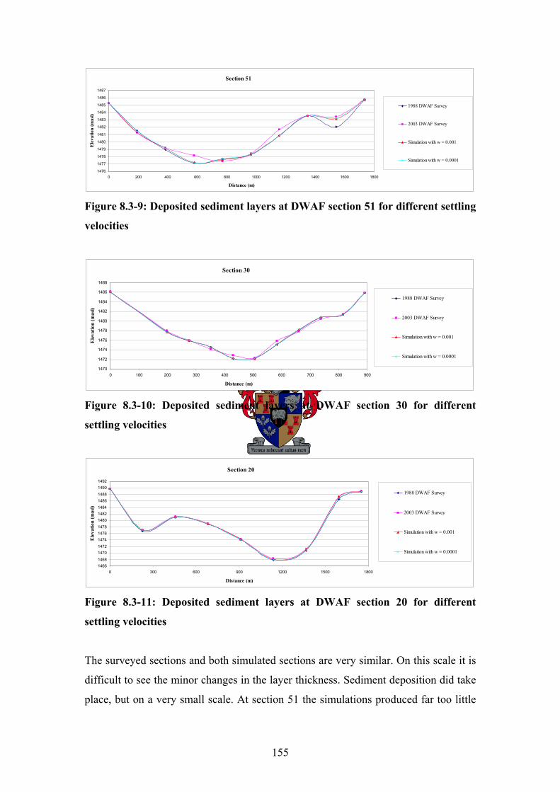
155

Section 51

1476

1477

1478

1479

1480

1481

1482

1483

1484

1485

1486

1487

0 200 400 600 800 1000 1200 1400 1600 1800

Distance (m)

Ele

vatio

n (m

asl)

1988 DWAF Survey

2003 DWAF Survey

Simulation with w = 0.001

Simulation with w = 0.0001

Figure 8.3-9: Deposited sediment layers at DWAF section 51 for different settling

velocities

Section 30

1470

1472

1474

1476

1478

1480

1482

1484

1486

1488

0 100 200 300 400 500 600 700 800 900

Distance (m)

Ele

vatio

n (m

asl)

1988 DWAF Survey

2003 DWAF Survey

Simulation with w = 0.001

Simulation with w = 0.0001

Figure 8.3-10: Deposited sediment layers at DWAF section 30 for different

settling velocities

Section 20

14661468147014721474147614781480148214841486148814901492

0 300 600 900 1200 1500 1800

Distance (m)

Ele

vatio

n (m

asl)

1988 DWAF Survey

2003 DWAF Survey

Simulation with w = 0.001

Simulation with w = 0.0001

Figure 8.3-11: Deposited sediment layers at DWAF section 20 for different

settling velocities

The surveyed sections and both simulated sections are very similar. On this scale it is

difficult to see the minor changes in the layer thickness. Sediment deposition did take

place, but on a very small scale. At section 51 the simulations produced far too little

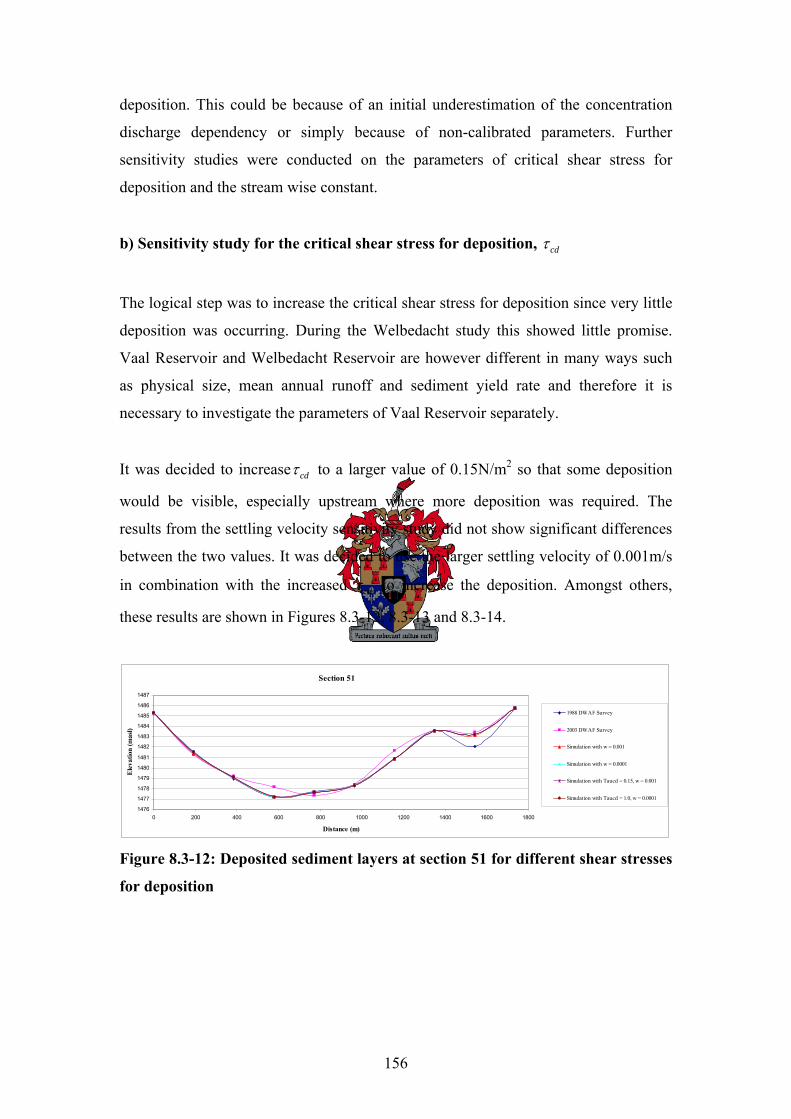
156

deposition. This could be because of an initial underestimation of the concentration

discharge dependency or simply because of non-calibrated parameters. Further

sensitivity studies were conducted on the parameters of critical shear stress for

deposition and the stream wise constant.

b) Sensitivity study for the critical shear stress for deposition, cdτ

The logical step was to increase the critical shear stress for deposition since very little

deposition was occurring. During the Welbedacht study this showed little promise.

Vaal Reservoir and Welbedacht Reservoir are however different in many ways such

as physical size, mean annual runoff and sediment yield rate and therefore it is

necessary to investigate the parameters of Vaal Reservoir separately.

It was decided to increase cdτ to a larger value of 0.15N/m2 so that some deposition

would be visible, especially upstream where more deposition was required. The

results from the settling velocity sensitivity study did not show significant differences

between the two values. It was decided to use the larger settling velocity of 0.001m/s

in combination with the increased cdτ to increase the deposition. Amongst others,

these results are shown in Figures 8.3-12, 8.3-13 and 8.3-14.

Section 51

1476

1477

1478

1479

1480

1481

1482

1483

1484

1485

1486

1487

0 200 400 600 800 1000 1200 1400 1600 1800

Distance (m)

Ele

vatio

n (m

asl)

1988 DWAF Survey

2003 DWAF Survey

Simulation with w = 0.001

Simulation with w = 0.0001

Simulation with Taucd = 0.15, w = 0.001

Simulation with Taucd = 1.0, w = 0.0001

Figure 8.3-12: Deposited sediment layers at section 51 for different shear stresses

for deposition

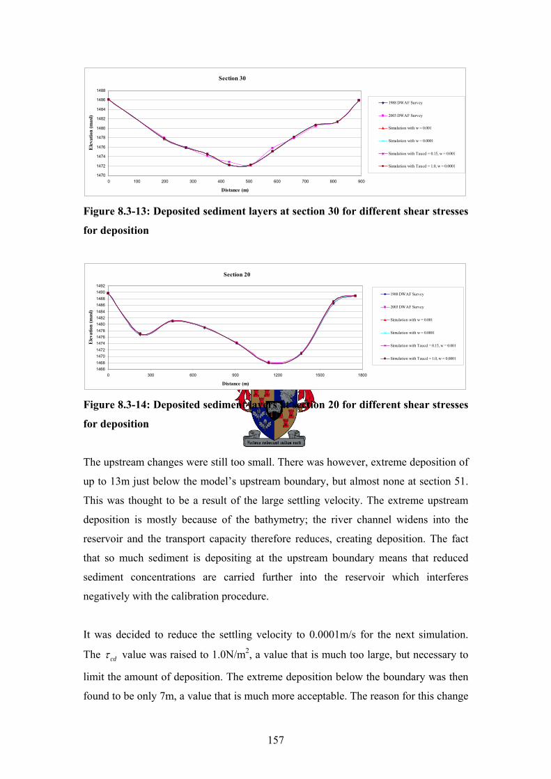
157

Section 30

1470

1472

1474

1476

1478

1480

1482

1484

1486

1488

0 100 200 300 400 500 600 700 800 900

Distance (m)

Ele

vatio

n (m

asl)

1988 DWAF Survey

2003 DWAF Survey

Simulation with w = 0.001

Simulation with w = 0.0001

Simulation with Taucd = 0.15, w = 0.001

Simulation with Taucd = 1.0, w = 0.0001

Figure 8.3-13: Deposited sediment layers at section 30 for different shear stresses

for deposition

Section 20

14661468147014721474147614781480148214841486148814901492

0 300 600 900 1200 1500 1800

Distance (m)

Ele

vatio

n (m

asl)

1988 DWAF Survey

2003 DWAF Survey

Simulation with w = 0.001

Simulation with w = 0.0001

Simulation with Taucd = 0.15, w = 0.001

Simulation with Taucd = 1.0, w = 0.0001

Figure 8.3-14: Deposited sediment layers at section 20 for different shear stresses

for deposition

The upstream changes were still too small. There was however, extreme deposition of

up to 13m just below the model’s upstream boundary, but almost none at section 51.

This was thought to be a result of the large settling velocity. The extreme upstream

deposition is mostly because of the bathymetry; the river channel widens into the

reservoir and the transport capacity therefore reduces, creating deposition. The fact

that so much sediment is depositing at the upstream boundary means that reduced

sediment concentrations are carried further into the reservoir which interferes

negatively with the calibration procedure.

It was decided to reduce the settling velocity to 0.0001m/s for the next simulation.

The cdτ value was raised to 1.0N/m2, a value that is much too large, but necessary to

limit the amount of deposition. The extreme deposition below the boundary was then

found to be only 7m, a value that is much more acceptable. The reason for this change

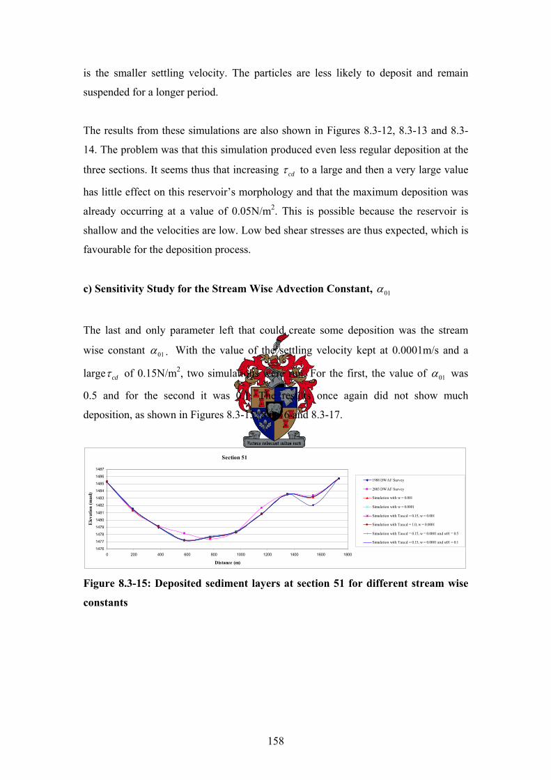
158

is the smaller settling velocity. The particles are less likely to deposit and remain

suspended for a longer period.

The results from these simulations are also shown in Figures 8.3-12, 8.3-13 and 8.3-

14. The problem was that this simulation produced even less regular deposition at the

three sections. It seems thus that increasing cdτ to a large and then a very large value

has little effect on this reservoir’s morphology and that the maximum deposition was

already occurring at a value of 0.05N/m2. This is possible because the reservoir is

shallow and the velocities are low. Low bed shear stresses are thus expected, which is

favourable for the deposition process.

c) Sensitivity Study for the Stream Wise Advection Constant, 01α

The last and only parameter left that could create some deposition was the stream

wise constant 01α . With the value of the settling velocity kept at 0.0001m/s and a

large cdτ of 0.15N/m2, two simulations were run. For the first, the value of 01α was

0.5 and for the second it was 0.1. The results once again did not show much

deposition, as shown in Figures 8.3-15, 8.3-16 and 8.3-17.

Section 51

1476

1477

1478

1479

1480

1481

1482

1483

1484

1485

1486

1487

0 200 400 600 800 1000 1200 1400 1600 1800

Distance (m)

Ele

vatio

n (m

asl)

1988 DWAF Survey

2003 DWAF Survey

Simulation with w = 0.001

Simulation with w = 0.0001

Simulation with Taucd = 0.15, w = 0.001

Simulation with Taucd = 1.0, w = 0.0001

Simulation with Taucd = 0.15, w = 0.0001 and α01 = 0.5

Simulation with Taucd = 0.15, w = 0.0001 and α01 = 0.1

Figure 8.3-15: Deposited sediment layers at section 51 for different stream wise

constants

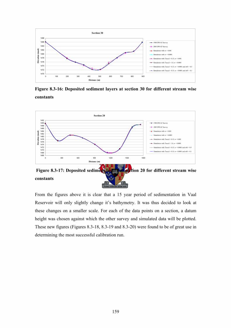
159

Section 30

1470

1472

1474

1476

1478

1480

1482

1484

1486

1488

0 100 200 300 400 500 600 700 800 900

Distance (m)

Ele

vatio

n (m

asl)

1988 DWAF Survey

2003 DWAF Survey

Simulation with w = 0.001

Simulation with w = 0.0001

Simulation with Taucd = 0.15, w = 0.001

Simulation with Taucd = 1.0, w = 0.0001

Simulation with Taucd = 0.15, w = 0.0001 and α01 = 0.5

Simulation with Taucd = 0.15, w = 0.0001 and α01 = 0.1

Figure 8.3-16: Deposited sediment layers at section 30 for different stream wise

constants

Section 20

14661468147014721474147614781480148214841486148814901492

0 300 600 900 1200 1500 1800

Distance (m)

Ele

vatio

n (m

asl)

1988 DWAF Survey

2003 DWAF Survey

Simulation with w = 0.001

Simulation with w = 0.0001

Simulation with Taucd = 0.15, w = 0.001

Simulation with Taucd = 1.0, w = 0.0001

Simulation with Taucd = 0.15, w = 0.0001 and α01 = 0.5

Simulation with Taucd = 0.15, w = 0.0001 and α01 = 0.1

Figure 8.3-17: Deposited sediment layers at section 20 for different stream wise

constants

From the figures above it is clear that a 15 year period of sedimentation in Vaal

Reservoir will only slightly change it’s bathymetry. It was thus decided to look at

these changes on a smaller scale. For each of the data points on a section, a datum

height was chosen against which the other survey and simulated data will be plotted.

These new figures (Figures 8.3-18, 8.3-19 and 8.3-20) were found to be of great use in

determining the most successful calibration run.

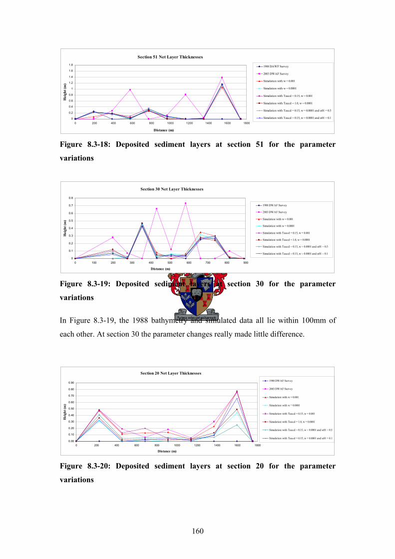
160

Section 51 Net Layer Thicknesses

0

0.2

0.4

0.6

0.8

1

1.2

1.4

1.6

1.8

0 200 400 600 800 1000 1200 1400 1600 1800

Distance (m)

Hei

ght (

m)

1988 DAWF Survey

2003 DWAF Survey

Simulation with w = 0.001

Simulation with w = 0.0001

Simulation with Taucd = 0.15, w = 0.001

Simulation with Taucd = 1.0, w = 0.0001

Simulation with Taucd = 0.15, w = 0.0001 and α01 = 0.5

Simulation with Taucd = 0.15, w = 0.0001 and α01 = 0.1

Figure 8.3-18: Deposited sediment layers at section 51 for the parameter

variations

Section 30 Net Layer Thicknesses

0

0.1

0.2

0.3

0.4

0.5

0.6

0.7

0.8

0 100 200 300 400 500 600 700 800 900

Distance (m)

Hei

ght (

m)

1988 DWAF Survey

2003 DWAF Survey

Simulation with w = 0.001

Simulation with w = 0.0001

Simulation with Taucd = 0.15, w = 0.001

Simulation with Taucd = 1.0, w = 0.0001

Simulation with Taucd = 0.15, w = 0.0001 and α01 = 0.5

Simulation with Taucd = 0.15, w = 0.0001 and α01 = 0.1

Figure 8.3-19: Deposited sediment layers at section 30 for the parameter

variations

In Figure 8.3-19, the 1988 bathymetry and simulated data all lie within 100mm of

each other. At section 30 the parameter changes really made little difference.

Section 20 Net Layer Thicknesses

0.00

0.10

0.20

0.30

0.40

0.50

0.60

0.70

0.80

0.90

0 200 400 600 800 1000 1200 1400 1600 1800

Distance (m)

Hei

ght (

m)

1988 DWAF Survey

2003 DWAF Survey

Simulation with w = 0.001

Simulation with w = 0.0001

Simulation with Taucd = 0.15, w = 0.001

Simulation with Taucd = 1.0, w = 0.0001

Simulation with Taucd = 0.15, w = 0.0001 and α01 = 0.5

Simulation with Taucd = 0.15, w = 0.0001 and α01 = 0.1

Figure 8.3-20: Deposited sediment layers at section 20 for the parameter

variations

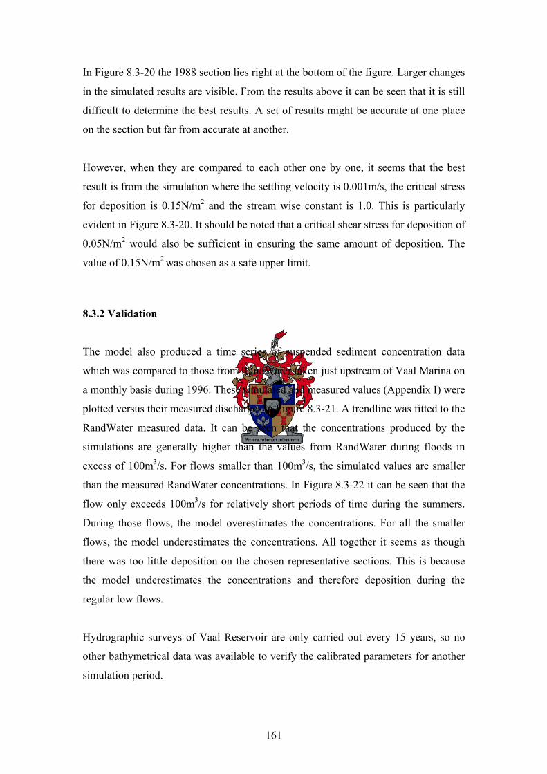
161

In Figure 8.3-20 the 1988 section lies right at the bottom of the figure. Larger changes

in the simulated results are visible. From the results above it can be seen that it is still

difficult to determine the best results. A set of results might be accurate at one place

on the section but far from accurate at another.

However, when they are compared to each other one by one, it seems that the best

result is from the simulation where the settling velocity is 0.001m/s, the critical stress

for deposition is 0.15N/m2 and the stream wise constant is 1.0. This is particularly

evident in Figure 8.3-20. It should be noted that a critical shear stress for deposition of

0.05N/m2 would also be sufficient in ensuring the same amount of deposition. The

value of 0.15N/m2 was chosen as a safe upper limit.

8.3.2 Validation The model also produced a time series of suspended sediment concentration data

which was compared to those from RandWater taken just upstream of Vaal Marina on

a monthly basis during 1996. These simulated and measured values (Appendix I) were

plotted versus their measured discharges in Figure 8.3-21. A trendline was fitted to the

RandWater measured data. It can be seen that the concentrations produced by the

simulations are generally higher than the values from RandWater during floods in

excess of 100m3/s. For flows smaller than 100m3/s, the simulated values are smaller

than the measured RandWater concentrations. In Figure 8.3-22 it can be seen that the

flow only exceeds 100m3/s for relatively short periods of time during the summers.

During those flows, the model overestimates the concentrations. For all the smaller

flows, the model underestimates the concentrations. All together it seems as though

there was too little deposition on the chosen representative sections. This is because

the model underestimates the concentrations and therefore deposition during the

regular low flows.

Hydrographic surveys of Vaal Reservoir are only carried out every 15 years, so no

other bathymetrical data was available to verify the calibrated parameters for another

simulation period.

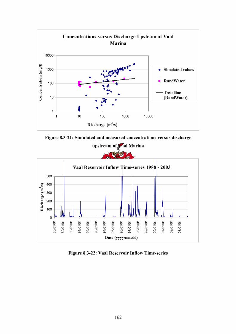
162

Concentrations versus Discharge Upsteam of Vaal Marina

1

10

100

1000

10000

1 10 100 1000 10000

Discharge (m3/s)

Con

cent

ratio

n (m

g/l)

Simulated values

RandWater

Trendline(RandWater)

Figure 8.3-21: Simulated and measured concentrations versus discharge

upstream of Vaal Marina

Vaal Reservoir Inflow Time-series 1988 - 2003

0

100

200

300

400

500

88/0

1/01

89/0

1/01

90/0

1/01

91/0

1/01

92/0

1/01

93/0

1/01

94/0

1/01

95/0

1/01

96/0

1/01

97/0

1/01

98/0

1/01

99/0

1/01

00/0

1/01

01/0

1/01

02/0

1/01

03/0

1/01

Date (yyyy/mm/dd)

Disc

harg

e (m

3 /s)

Figure 8.3-22: Vaal Reservoir Inflow Time-series

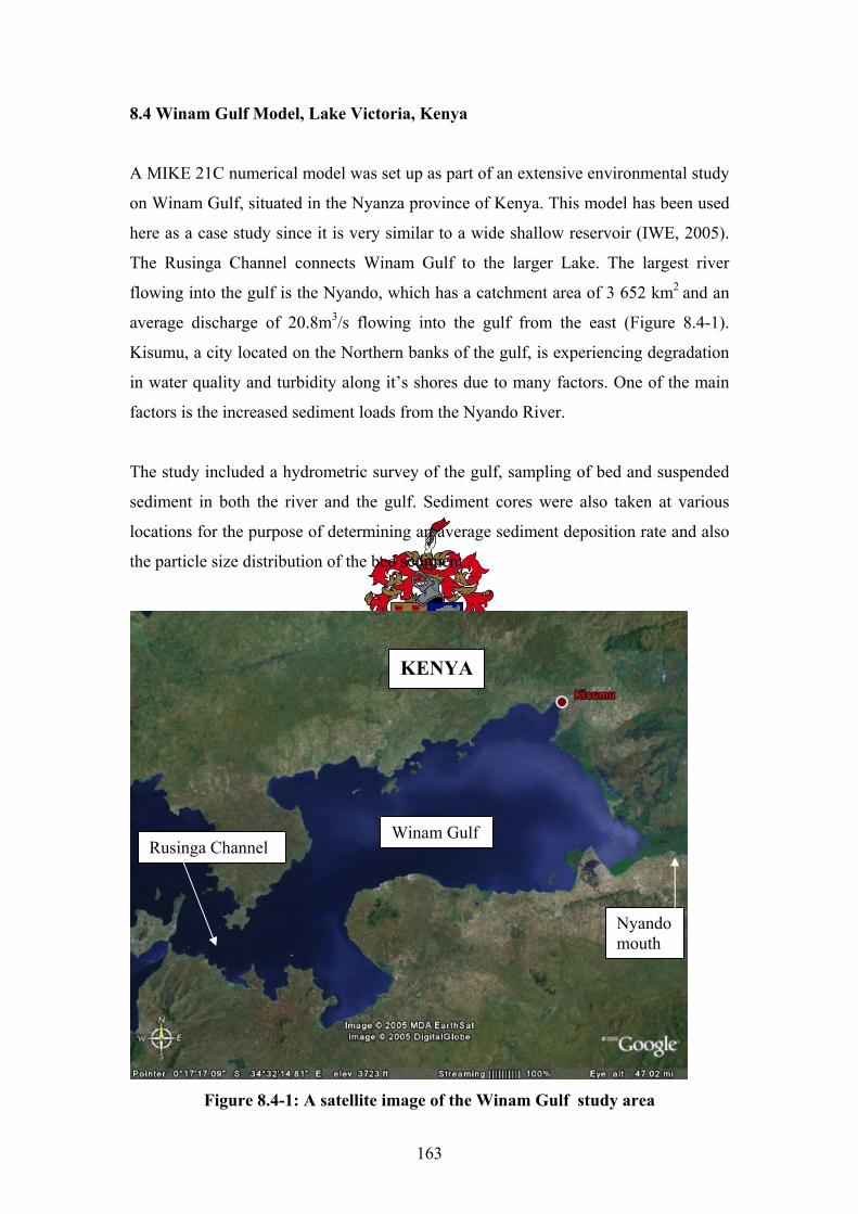
163

8.4 Winam Gulf Model, Lake Victoria, Kenya

A MIKE 21C numerical model was set up as part of an extensive environmental study

on Winam Gulf, situated in the Nyanza province of Kenya. This model has been used

here as a case study since it is very similar to a wide shallow reservoir (IWE, 2005).

The Rusinga Channel connects Winam Gulf to the larger Lake. The largest river

flowing into the gulf is the Nyando, which has a catchment area of 3 652 km2 and an

average discharge of 20.8m3/s flowing into the gulf from the east (Figure 8.4-1).

Kisumu, a city located on the Northern banks of the gulf, is experiencing degradation

in water quality and turbidity along it’s shores due to many factors. One of the main

factors is the increased sediment loads from the Nyando River.

The study included a hydrometric survey of the gulf, sampling of bed and suspended

sediment in both the river and the gulf. Sediment cores were also taken at various

locations for the purpose of determining an average sediment deposition rate and also

the particle size distribution of the bed sediment.

Figure 8.4-1: A satellite image of the Winam Gulf study area

Winam Gulf

Nyando mouth

Rusinga Channel

KENYA

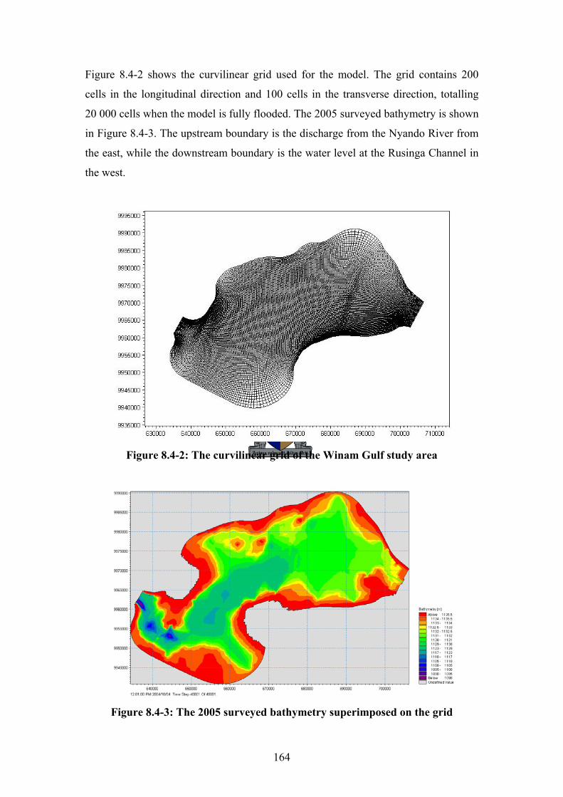
164

Figure 8.4-2 shows the curvilinear grid used for the model. The grid contains 200

cells in the longitudinal direction and 100 cells in the transverse direction, totalling

20 000 cells when the model is fully flooded. The 2005 surveyed bathymetry is shown

in Figure 8.4-3. The upstream boundary is the discharge from the Nyando River from

the east, while the downstream boundary is the water level at the Rusinga Channel in

the west.

Figure 8.4-2: The curvilinear grid of the Winam Gulf study area

Figure 8.4-3: The 2005 surveyed bathymetry superimposed on the grid

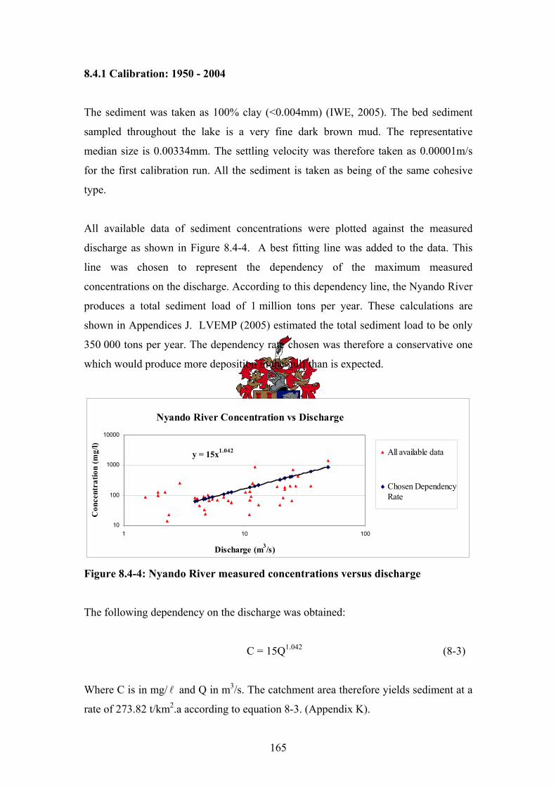
165

8.4.1 Calibration: 1950 - 2004

The sediment was taken as 100% clay (<0.004mm) (IWE, 2005). The bed sediment

sampled throughout the lake is a very fine dark brown mud. The representative

median size is 0.00334mm. The settling velocity was therefore taken as 0.00001m/s

for the first calibration run. All the sediment is taken as being of the same cohesive

type.

All available data of sediment concentrations were plotted against the measured

discharge as shown in Figure 8.4-4. A best fitting line was added to the data. This

line was chosen to represent the dependency of the maximum measured

concentrations on the discharge. According to this dependency line, the Nyando River

produces a total sediment load of 1 million tons per year. These calculations are

shown in Appendices J. LVEMP (2005) estimated the total sediment load to be only

350 000 tons per year. The dependency rate chosen was therefore a conservative one

which would produce more deposition in the gulf than is expected.

Nyando River Concentration vs Discharge

y = 15x1.042

10

100

1000

10000

1 10 100

Discharge (m3/s)

Con

cent

ratio

n (m

g/l)

All available data

Chosen DependencyRate

Figure 8.4-4: Nyando River measured concentrations versus discharge

The following dependency on the discharge was obtained:

C = 15Q1.042 (8-3)

Where C is in mg/ l and Q in m3/s. The catchment area therefore yields sediment at a

rate of 273.82 t/km2.a according to equation 8-3. (Appendix K).

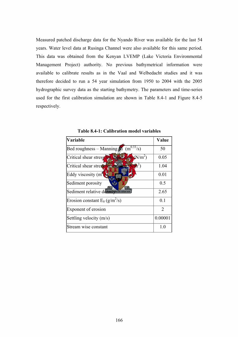
166

Measured patched discharge data for the Nyando River was available for the last 54

years. Water level data at Rusinga Channel were also available for this same period.

This data was obtained from the Kenyan LVEMP (Lake Victoria Environmental

Management Project) authority. No previous bathymetrical information were

available to calibrate results as in the Vaal and Welbedacht studies and it was

therefore decided to run a 54 year simulation from 1950 to 2004 with the 2005

hydrographic survey data as the starting bathymetry. The parameters and time-series

used for the first calibration simulation are shown in Table 8.4-1 and Figure 8.4-5

respectively.

Table 8.4-1: Calibration model variables

Variable Value

Bed roughness – Manning M (m0.33/s) 50

Critical shear stress for deposition (N/m2) 0.05

Critical shear stress for erosion (N/m2) 1.04

Eddy viscosity (m2/s) 0.01

Sediment porosity 0.5

Sediment relative density 2.65

Erosion constant E0 (g/m2/s) 0.1

Exponent of erosion 2

Settling velocity (m/s) 0.00001

Stream wise constant 1.0

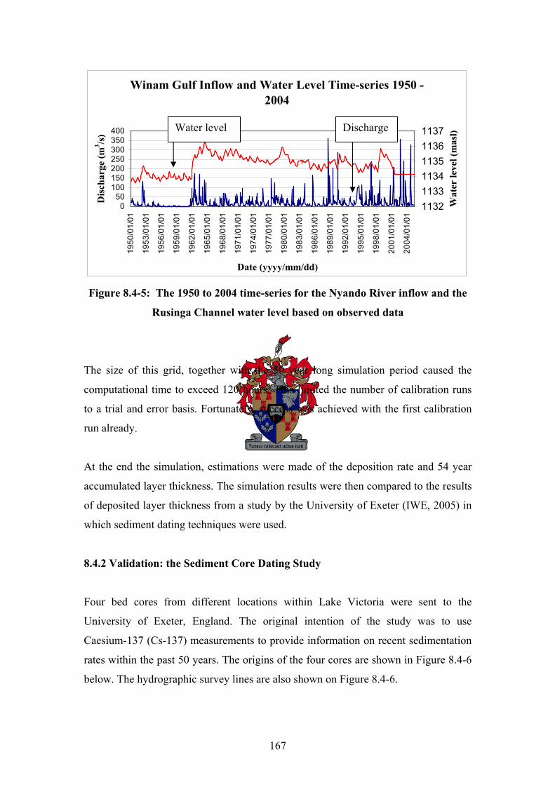
167

Winam Gulf Inflow and Water Level Time-series 1950 - 2004

050

100150200250300350400

1950

/01/

01

1953

/01/

01

1956

/01/

01

1959

/01/

01

1962

/01/

01

1965

/01/

01

1968

/01/

01

1971

/01/

01

1974

/01/

01

1977

/01/

01

1980

/01/

01

1983

/01/

01

1986

/01/

01

1989

/01/

01

1992

/01/

01

1995

/01/

01

1998

/01/

01

2001

/01/

01

2004

/01/

01

Date (yyyy/mm/dd)

Disc

harg

e (m

3 /s)

113211331134113511361137

Wat

er le

vel (

mas

l)

Figure 8.4-5: The 1950 to 2004 time-series for the Nyando River inflow and the

Rusinga Channel water level based on observed data

The size of this grid, together with the 50 year long simulation period caused the

computational time to exceed 120 hours. This limited the number of calibration runs

to a trial and error basis. Fortunately, success was achieved with the first calibration

run already.

At the end the simulation, estimations were made of the deposition rate and 54 year

accumulated layer thickness. The simulation results were then compared to the results

of deposited layer thickness from a study by the University of Exeter (IWE, 2005) in

which sediment dating techniques were used.

8.4.2 Validation: the Sediment Core Dating Study

Four bed cores from different locations within Lake Victoria were sent to the

University of Exeter, England. The original intention of the study was to use

Caesium-137 (Cs-137) measurements to provide information on recent sedimentation

rates within the past 50 years. The origins of the four cores are shown in Figure 8.4-6

below. The hydrographic survey lines are also shown on Figure 8.4-6.

Discharge Water level

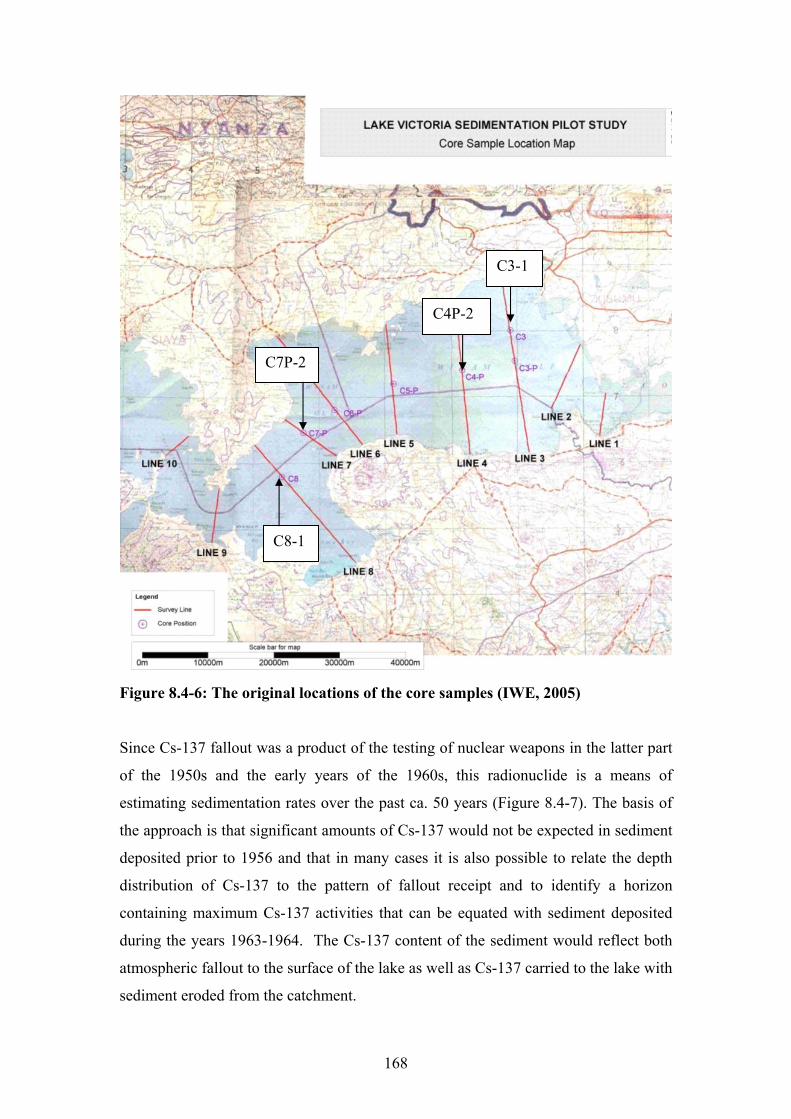
168

Figure 8.4-6: The original locations of the core samples (IWE, 2005)

Since Cs-137 fallout was a product of the testing of nuclear weapons in the latter part

of the 1950s and the early years of the 1960s, this radionuclide is a means of

estimating sedimentation rates over the past ca. 50 years (Figure 8.4-7). The basis of

the approach is that significant amounts of Cs-137 would not be expected in sediment

deposited prior to 1956 and that in many cases it is also possible to relate the depth

distribution of Cs-137 to the pattern of fallout receipt and to identify a horizon

containing maximum Cs-137 activities that can be equated with sediment deposited

during the years 1963-1964. The Cs-137 content of the sediment would reflect both

atmospheric fallout to the surface of the lake as well as Cs-137 carried to the lake with

sediment eroded from the catchment.

C8-1

C3-1

C4P-2

C7P-2

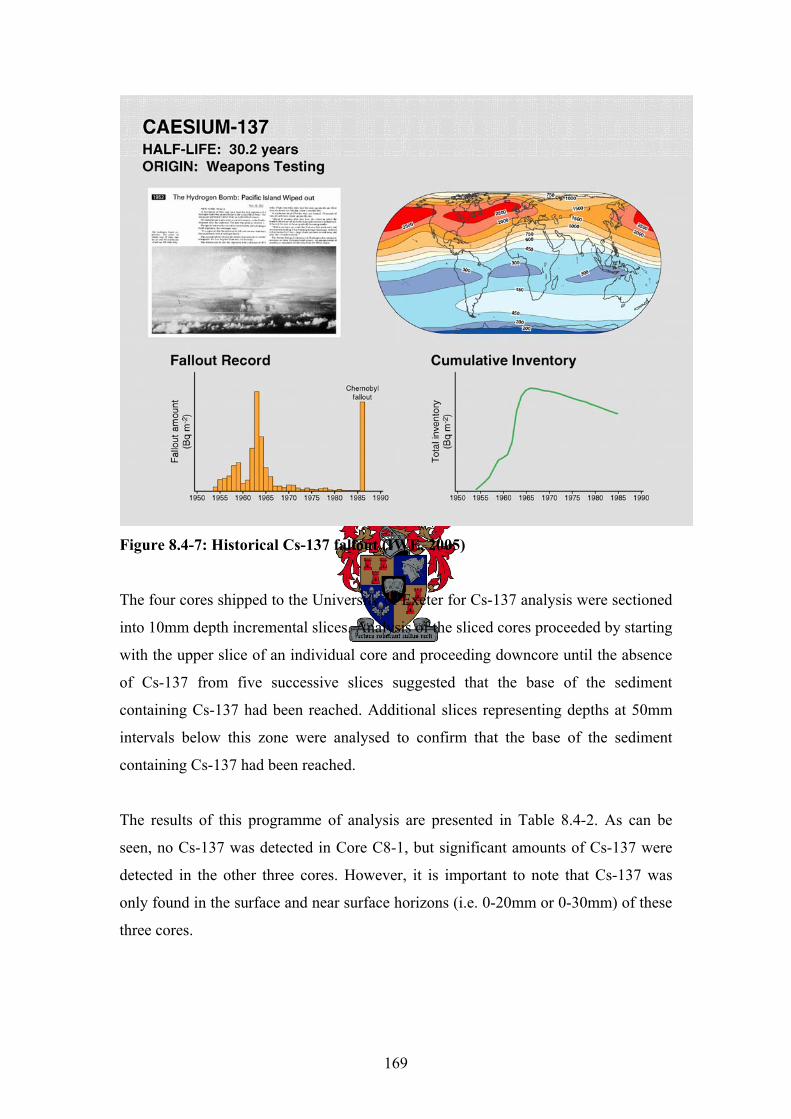
169

Figure 8.4-7: Historical Cs-137 fallout (IWE, 2005)

The four cores shipped to the University of Exeter for Cs-137 analysis were sectioned

into 10mm depth incremental slices. Analysis of the sliced cores proceeded by starting

with the upper slice of an individual core and proceeding downcore until the absence

of Cs-137 from five successive slices suggested that the base of the sediment

containing Cs-137 had been reached. Additional slices representing depths at 50mm

intervals below this zone were analysed to confirm that the base of the sediment

containing Cs-137 had been reached.

The results of this programme of analysis are presented in Table 8.4-2. As can be

seen, no Cs-137 was detected in Core C8-1, but significant amounts of Cs-137 were

detected in the other three cores. However, it is important to note that Cs-137 was

only found in the surface and near surface horizons (i.e. 0-20mm or 0-30mm) of these

three cores.

170

The data presented in Table 8.4-2 can be used to make a number of inferences

regarding sedimentation rates at the sites from which the cores were collected. These

are as follows:

a) Sedimentation rates are relatively low, with the rates estimated for the four

cores containing Cs-137 lying in the range 20-30cm in 50 years.

b) The absence of measurable Cs-137 from core C8-1 suggests that little or no

sediment accumulation has occurred at this site in the past 50 years.

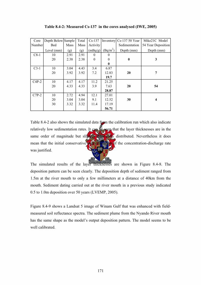
171

Table 8.4-2: Measured Cs-137 in the cores analysed (IWE, 2005)

Core Depth Below Sample Total Cs-137 Inventory Cs-137 50 Year Mike21C Model Number Bed Mass Mass Activity Sedimentation 54 Year Deposition

Level (mm) (g) (g) (mBq/g) (Bq/m2) Depth (mm) Depth (mm)C8-1 10 2.91 2.91 0 0

20 2.38 2.38 0 0 0 30

C3-1 10 3.04 4.43 3.4 6.8720 3.92 3.92 7.2 12.83 20 7

19.7C4P-2 10 4.17 4.17 11.2 21.25

20 4.33 4.33 3.9 7.63 20 5428.87

C7P-2 10 2.72 4.94 12.1 27.0120 3.04 3.04 9.1 12.52 30 430 3.32 3.32 11.4 17.19

56.71

Table 8.4-2 also shows the simulated data from the calibration run which also indicate

relatively low sedimentation rates. It can be seen that the layer thicknesses are in the

same order of magnitude but slightly differently distributed. Nevertheless it does

mean that the initial conservative overestimation of the concentration-discharge rate

was justified.

The simulated results of the layer thicknesses are shown in Figure 8.4-8. The

deposition pattern can be seen clearly. The deposition depth of sediment ranged from

1.5m at the river mouth to only a few millimeters at a distance of 40km from the

mouth. Sediment dating carried out at the river mouth in a previous study indicated

0.5 to 1.0m deposition over 50 years (LVEMP, 2005).

Figure 8.4-9 shows a Landsat 5 image of Winam Gulf that was enhanced with field-

measured soil reflectance spectra. The sediment plume from the Nyando River mouth

has the same shape as the model’s output deposition pattern. The model seems to be

well calibrated.

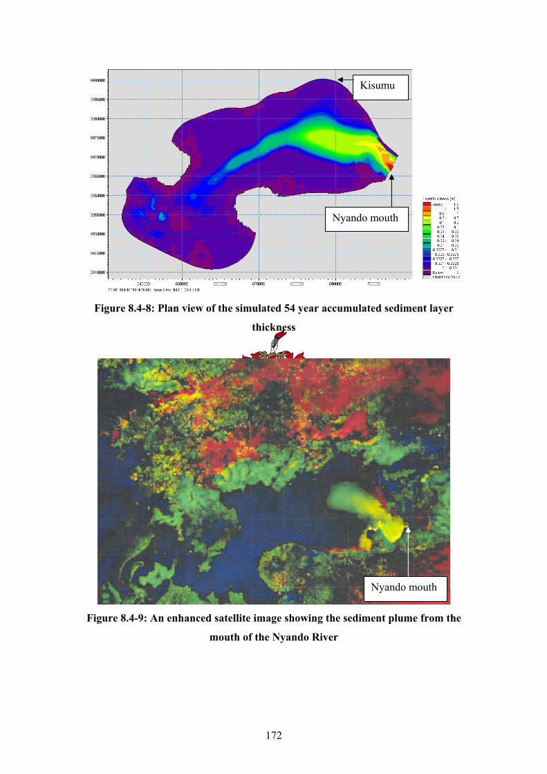
172

Figure 8.4-8: Plan view of the simulated 54 year accumulated sediment layer

thickness

Figure 8.4-9: An enhanced satellite image showing the sediment plume from the

mouth of the Nyando River

Kisumu

Nyando mouth

Nyando mouth

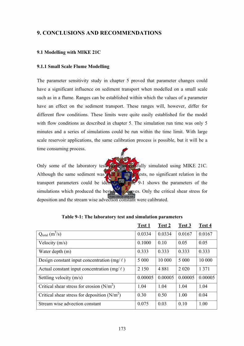
173

9. CONCLUSIONS AND RECOMMENDATIONS

9.1 Modelling with MIKE 21C

9.1.1 Small Scale Flume Modelling

The parameter sensitivity study in chapter 5 proved that parameter changes could

have a significant influence on sediment transport when modelled on a small scale

such as in a flume. Ranges can be established within which the values of a parameter

have an effect on the sediment transport. These ranges will, however, differ for

different flow conditions. These limits were quite easily established for the model

with flow conditions as described in chapter 5. The simulation run time was only 5

minutes and a series of simulations could be run within the time limit. With large

scale reservoir applications, the same calibration process is possible, but it will be a

time consuming process.

Only some of the laboratory tests were successfully simulated using MIKE 21C.

Although the same sediment was used in all the tests, no significant relation in the

transport parameters could be identified. Table 9-1 shows the parameters of the

simulations which produced the best fitting curves. Only the critical shear stress for

deposition and the stream wise advection constant were calibrated.

Table 9-1: The laboratory test and simulation parameters

Test 1 Test 2 Test 3 Test 4

Qtotal (m3/s) 0.0334 0.0334 0.0167 0.0167

Velocity (m/s) 0.1000 0.10 0.05 0.05

Water depth (m) 0.333 0.333 0.333 0.333

Design constant input concentration (mg/ l ) 5 000 10 000 5 000 10 000

Actual constant input concentration (mg/ l ) 2 150 4 881 2 020 1 371

Settling velocity (m/s) 0.00005 0.00005 0.00005 0.00005

Critical shear stress for erosion (N/m2) 1.04 1.04 1.04 1.04

Critical shear stress for deposition (N/m2) 0.30 0.50 1.00 0.04

Stream wise advection constant 0.075 0.03 0.10 1.00

174

It was decided to disregard the results from Test 3 because of the drastic fall in

sediment concentration between the distances of 10m and 15m. The results are

unrealistic and there probably was as error in the sampling or analysis procedures for

this test. The critical shear stress for deposition for this test was also found to be much

too high compared to the other tests.

It must be borne in mind that Tests 1 and 2 have the same flow depth, but double the

discharge of Test 4. It is therefore unlikely that a single set of values for the two

adjusted parameters will be identified that could create numerical results for all 4 tests

that compares to the lab results.

The resultant curves from the simulations do compare to the curves from the

laboratory tests, especially for Tests 1 and 4. The parameter values, however, do not

compare.

It can be seen that the two parameters that were adjusted, cdτ and 01α , vary

significantly between Tests 1, 2 and 4. These values for Test 1 and 2 are comparable.

The low values of 01α used in both Tests 1 and 2 indicate that the transport

mechanism could well have been a density current and not turbulent suspension after

all. This can also be seen in the drastic changes between the design constant input

concentrations and the measured laboratory upstream concentrations. The sediment

probably formed a density current which dived underneath the sampling instruments.

The result was that lower weighted average concentrations were calculated at each

sampling station for each test due to the assumed turbulent velocity distribution,

producing unreliable results.

9.1.2 Large Scale Reservoir Modelling

When narrow reservoirs with relatively fast flowing water and high sediment loads

are modelled, the effects of parameter changes are immediately visible when sections

are plotted. This was the case with the Welbedacht Reservoir model.

175

Initially it seemed as though changes of the sediment transport parameters became

almost insignificant for a large reservoir with a low average sediment load. This was

really because the sediment layer is spread out over the width and length of the

reservoir and the layer is thus much thinner and less visible. Changes of the transport

parameters will cause differences in the sedimentation. These will however be less

visible and they can sometimes only be observed and analysed on a smaller scale.

When large reservoirs, such as Vaal Reservoir, are modelled, large sediment deposits

are found at the upstream boundary already. This is because the sediment enters into a

flow with a low sediment transport capacity and thus is deposited. This low transport

capacity is because of the low flow velocities caused by the damming and the sudden

increase in width and depth of the flow area as the river enters the reservoir. This can

be prevented by changing the bathymetry at the upstream boundary to a channel with

an increasing sectional area so that the widening towards the reservoir is more

gradual. The sediment will then deposit more gradually along the channel and into the

reservoir. It must be kept in mind that the channel must still be able to handle the

largest expected flood without the banks being overtopped. This will cause the

simulation to become unstable. The parameters that were used in the reservoir models

are shown in Table 9-2.

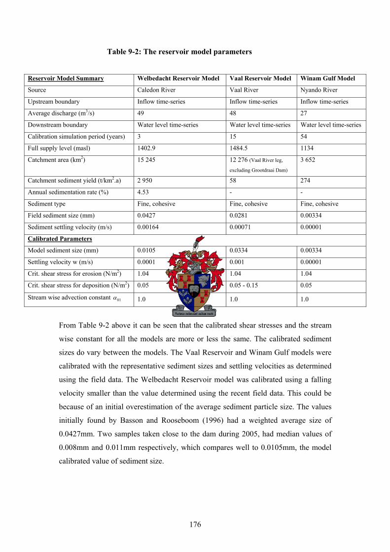
176

Table 9-2: The reservoir model parameters

Reservoir Model Summary Welbedacht Reservoir Model Vaal Reservoir Model Winam Gulf Model

Source Caledon River Vaal River Nyando River

Upstream boundary Inflow time-series Inflow time-series Inflow time-series

Average discharge (m3/s) 49 48 27

Downstream boundary Water level time-series Water level time-series Water level time-series

Calibration simulation period (years) 3 15 54

Full supply level (masl) 1402.9 1484.5 1134

Catchment area (km2) 15 245 12 276 (Vaal River leg,

excluding Grootdraai Dam) 3 652

Catchment sediment yield (t/km2.a) 2 950 58 274

Annual sedimentation rate (%) 4.53 - -

Sediment type Fine, cohesive Fine, cohesive Fine, cohesive

Field sediment size (mm) 0.0427 0.0281 0.00334

Sediment settling velocity (m/s) 0.00164 0.00071 0.00001

Calibrated Parameters

Model sediment size (mm) 0.0105 0.0334 0.00334

Settling velocity w (m/s) 0.0001 0.001 0.00001

Crit. shear stress for erosion (N/m2) 1.04 1.04 1.04

Crit. shear stress for deposition (N/m2) 0.05 0.05 - 0.15 0.05

Stream wise advection constant 01α 1.0 1.0 1.0

From Table 9-2 above it can be seen that the calibrated shear stresses and the stream

wise constant for all the models are more or less the same. The calibrated sediment

sizes do vary between the models. The Vaal Reservoir and Winam Gulf models were

calibrated with the representative sediment sizes and settling velocities as determined

using the field data. The Welbedacht Reservoir model was calibrated using a falling

velocity smaller than the value determined using the recent field data. This could be

because of an initial overestimation of the average sediment particle size. The values

initially found by Basson and Rooseboom (1996) had a weighted average size of

0.0427mm. Two samples taken close to the dam during 2005, had median values of

0.008mm and 0.011mm respectively, which compares well to 0.0105mm, the model

calibrated value of sediment size.

177

9.2 Recommended Parameter Calibration Procedure 9.2.1 Sediment Size

The particle size grading of the sediment must be determined by sieve and hydrometer

analyses of field samples. These samples should be taken close to the dam especially

when the reservoir is silted up and operates like a run-of-river scheme, as proven in

the case for the Welbedacht Reservoir model. A representative particle size (median

or weighted average) is then used to calculate an expected average particle settling

velocity.

9.2.2 Settling Velocity In the case of reservoir models, the settling velocity calculated for a field sample’s

median or weighted average particle size can serve as a reliable parameter, as shown

by the reservoir models.

9.2.3 Critical Shear Stress for Deposition

Calculating Expected Minimum Bed Shear Stress It is recommended that firstly the reservoir model simulation is run for only

hydrodynamics and no morphological changes. The results from this simulation will

produce a minimum velocity at a certain time and place during the simulation. The

depth as that point can also be determined from the hydrodynamic output.

With this information available, the bed shear stress at that point can then be

calculated using the following equation:

( )2

21/ 6

gv

Mh

ρτ = (9-1)

where M is the user specified bed roughness.

178

The used values of velocity and depth should actually be from the point of which the

combination of velocity and depth produces the lowest bed stress, and not the point

with the minimum velocity. To determine the point with the real minimum bed stress,

however, could be problematic, since MIKE 21C does not give bed stress as output.

This method will however still give a good approximation.

Knowing the expected minimum bed stress, the critical shear stress for deposition can

be set around this value and evaluated in a sensitivity study format as done in this

research. Any value larger than the expected minimum stress will produce some

deposition.

The sensitivity studies in chapter 8 however, started out using a critical shear stress

for deposition value that was recommended by Basson et al. (2003).

The minimum bed shear stress will, in effect, actually be 0N/m2. Some deposition will

always occur where suspended sediment is available and the bed stresses are very

low. The method to determine the minimum bed shear stress, as described above,

should only be applied to points within the main channel of the reservoir.

9.2.4 The Critical Shear Stress for Erosion

Calculating Expected Maximum Bed Stress There is still uncertainty about the parameter of critical shear stress for erosion. What

is recommended is that firstly the reservoir model simulation is run for only

hydrodynamics and no morphological changes, as described in the method to

determine the minimum bed shear stress. The results from this simulation will

produce a maximum velocity at a certain time and place during the simulation. The

depth as that point can also be determined from the hydrodynamic output.

With this information available, the bed shear stress at that point can then be

calculated using equation 9-1.

179

The used values of velocity and depth should actually be from the point of which the

combination of velocity and depth produces the largest bed stress, and not the point

with the largest velocity. To determine the point with the real maximum bed stress,

however, could be problematic, since MIKE 21C does not give bed stress as output.

As stated before, this method will however still give a good approximation.

This stress can then be accepted as the maximum limit stress for erosion to occur. Any

set value of the critical erosion stress below this value will produce erosion to a

certain extent. Any value set above this, will limit erosion. For the models used in this

research, little or no erosion was required and therefore the critical stress for erosion

was kept at a value larger than the expected bed stresses. Further studies are needed so

that the critical stress for erosion can be directly linked to cohesive bed sediment

characteristics.

9.2.5 Stream Wise Advection Constant

The stream wise constant should be 1.0 for reservoir models. This ensures uniform

distribution of the fine sediment over the depth and width of the section. It allows the

sediment to be transported deep into the reservoir, as is expected from fine cohesive

sediment. Reducing the value of 01α in reservoir models did not bring about more

deposition since the maximum velocities are then brought closer to the bed, creating

unfavourable conditions for deposition. In effect, erosion can occur because of the

increased flow velocities close the bed.

9.2.6 Calibration Data

It is recommended that as much as possible field data are collected prior to the

modelling of reservoir sedimentation. Any data related to the sedimentation can be of

use in creating a reliable model. This includes data from various hydrographic

surveys, measured data of discharge and water level, measured sediment

concentration data, measured field data, laboratory flume data and even satellite

images.

180

9.3 Research Recommendations

The recommended further research topics in this field that are:

Calibration of the latest MIKE 21C software with the fully adjustable

parameters of sediment transport and multi-fraction simulation capabilities.

Calibration of MIKE 21C flume model with the use of reliable laboratory data.

It is recommended to use lower sediment concentrations to prevent the

formation of a density current. Higher flow velocities will help create

turbulent transport.

Research into the determination of critical shear stresses for erosion of

cohesive sediments beds.

181

10. REFERENCES Armanini, A. and Di Silvio, G. (1988). A One-dimensional Model for the Transport of

a Sediment Mixture in Non-equilibrium Conditions. Journal of Hydraulic Research,

26 (3).

Arrifin, J. (2002). Evaluation of Equations on Total Bed Material Load. International

Conference on Urban Hydrology for the 21st Century, October 2002, Kuala Lumpur.

Basson, G.R. and de Villiers, J.W.L. (2005). New Bridge Across Caledon River:

Welbedacht Reservoir Sedimentation and Flood Level Study. ASP Technology (Pty)

Ltd.

Basson, G.R.; Havno, K.; Tjerry, S. and Olesen, K.W. (2003). Modelling

Sedimentation, Sluicing and Flushing in Shallow Reservoirs.

Basson, G.R., Melvill, J. and de Villiers, J.W.L. (2005). Vaal River Eastern Sub-

System Augmentation Project (VRESAP): Abstraction Works Hydraulic Model

Study. University of Stellenbosch Hydraulic Laboratory & ASP Technology (Pty)

Ltd.

Basson, G.R. and Olesen, K.W. (2004). Control of Reservoir Sedimentation by Flood

Flushing: Impacts, Operation and Mathematical Modelling.

Basson, G.R. and Rooseboom, A. (1997). Dealing with Reservoir Sedimentation.

Water Research Commission Report No. TT 91/97.

Batuca, D.G. and Jordaan, J.M. (2000). Silting and Desilting of Reservoirs. Balkema

Publishers, Rotterdam.

Beck, J.S. and Basson, G.R. (2003). The Hydraulics of the Impacts of Dam

Development on the River Morphology. Water Research Commission Report No.

1102/1/03.

182

Beck, J.S. and Basson, G.R. (2002). Morphological Impacts and Mitigation Measures:

Control of Reservoir Sedimentation and Environmental Flood Releases Short Course,

Department of Civil Engineering, University of Stellenbosch, South Africa.

Chadwick, A. and Morfett, J. (1998). Hydraulics in Civil and Environmental

Engineering - Third Edition. Spon Press, London.

Clark, J. (1990). Department of Water Affairs and Forestry - Vaal Dam Capacity

Determination 1986 – 1990. Report No. C120-01.

Clark, J. (1990). Department of Water Affairs and Forestry – Welbedacht Dam

Capacity Determination 1990. Report No. D200-01.

Craig, R.F. (2001). Soil Mechanics – Sixth Edition. Spon Press, London.

Cunge (1989). In Delft Hydraulics, 1992.

Cunge, J.A.; Holly, F.M. and Verwey, A. (1980). Practical Aspects of Computational

River Hydraulics. Pitman Publishing Inc., Boston, USA.

Di Silvio, G. (1995). River Modelling. UNESCO IHP-IV Project H-1-2, Working

Group on Erosion, Riverbed Deformation and Sediment Transport in River Basins as

Related to National and Manmade Changes.

Delft Hydraulics (1992). The Control of Reservoir Sedimentation – A Literature

Review. Ministry of Development Co-operation, Government of the Netherlands,

Delft Hydraulics.

De Vriend, H.J. (1981). Steady Flow in Shallow Channel Bends. Communications on

Hydraulics, 81-3. Delft University of Technology, The Netherlands.

Dou, G.R. (1963) Sediment Transport Theory. Nanjing Hydraulic Institute, China.

183

Dou, G.R. (1980). The Stochastic Theory and the General Law of all Flow Regions

for Turbulent Open Channel Flows. Proceedings of the First International Symposium

on River Sedimentation, China. Guanghua Press.

Dou, G.R.; Lu, Y.; Han, L.; Shao, X. and Yang, X. (2004). 3D Numerical Simulation

for Water Flows and Sediment Deposition in Dam Area of the Three Gorges Project.

Proceedings of the Ninth International Symposium on River Sedimentation, China.

DHI Water & Environment. (2001). MIKE 11, A Modelling System for Rivers and

Channels – User Guide.

DHI Water & Environment. (2003). MIKE 21C River Hydrodynamics and

Morphology – User Guide.

DHI Water & Environment. (2003). MIKE 21C River Morphology - A Short

Description.

DWAF (2006). www.dwaf.gov.za. Home Page of the Department of Water Affairs

and Forestry, South Africa.

Falconer, R.A. and Owens, P.H. (1990). Numerical Modelling of Suspended Sediment

Fluxes in Estuarine Waters. Estuarine, Coastal and Shelf Science Vol. 31.

Han, Q. (1980). A Study on the Non-equilibrium Transport of Suspended Sediment.

Proceedings of the First International Symposium on River Sedimentation, China.

Han, Q. and He, M. (1990). A Mathematical Model for Reservoir Sedimentation and

Fluvial Processes. International Journal of Sediment Research., IRTCES.

H.R. Wallingford (1998). Reservoir Sedimentation Management, Tarbela Dam. Water

and Power Development Authority.

184

Holly, F.M. and Cunge, J.A. (1975). Time Dependant Mass Dispersion in Natural

Streams. Proceedings of the Symposium on Modelling Techniques. American Society

of Civil Engineers, San Francisco.

IWE (2005). Pilot Study on Sedimentation and Sediment Characteristics on Nyando

and Nzoia River Mouths and Winam Gulf of Lake Victoria. Institute for Water and

Environmental Engineering, University of Stellenbosch.

Jia, Y. and Wang, S.S.Y. (1999). Numerical Model for Channel Flow and

Morphological Change Studies. Journal of Hydraulic Engineering, ASCE, Vol. 125

No. 9.

Jordaan, J.M. (1989). The Sediment Problem in South African Reservoirs.

Proceedings of the International Symposium on Sediment Transport Modelling, USA.

Karanshev (1963). In Delft Hydraulics, 1992.

Le Moigne, G. (1990). Dam Safety and the Environment. World Bank Technical

Paper No. 115.

Lin, B.N.; Huang, J. and Li, X. (1983). Unsteady Transport of Suspended Load at

Small Concentration. Journal of Hydraulic Engineering, ASCE, Vol. 109, No. 1.

Lin, B.N. and Shen, H. (1984). Two-dimensional Flow with Sediment by

Characteristics Method. Journal of Hydraulic Engineering, ASCE, Vol. 110, No. 5.

Lopez, J.L. (1978). Mathematical Modelling of Sediment Deposition in Reservoirs.

Ph.D. Dissertation . Colorado State University, USA.

LVEMP (2005). Lake Victoria Regional Water Quality Synthesis Report. October

2005.

185

Mehta, A.J. and Partheniades, E. (1973). Effects of Physico-chemical Properties of

Fine Suspended Sediment on the Degree of Deposition. Paper A-41. Proceedings of

the International Symposium on River Mechanics, Bangkok.

Olesen, K.W. and Basson, G.R. (2004). 1D and 2D Modelling of Sedimentation and

Flushing in Shallow Reservoirs. Proceedings of the Ninth International Symposium

on River Sedimentation, Yichang, China.

Palmieri, A. (2003). Social and Economic Aspects of Reservoir Conservation. World

Water Forum, Kyoto, Japan.

Postel, S. (1989). Water for Agriculture, Facing the Limits. World Watch Paper 93.

Rahuel, J.L. and Holly, F.M. (1989). Modelling of Riverbed Evolution for Bedload

Sediment Mixtures. Journal of Hydraulic Engineering, ASCE, 115 (11).

Rooseboom, A. (1975). Sediment Transport in Rivers and Reservoirs. D.Eng

Dissertation, University of Pretoria, (In Afrikaans). (Later Published by Water

Research Commission, South Africa, Report No. 297/1/92, English).

Rooseboom, A. (1992). Sediment Transport in Rivers and Reservoirs – A South

African Perspective. Water Research Commission Report No. 297/1/92.

Rooseboom, A. and Maas, N.F. (1974). Sedimentafvoer in die Oranje-, Tugela- en

Pongolariviere. Technical Report No. 59, Department of Water Affairs and Forestry.

Rooseboom, A. and Mulke, F.J. (1982). Recent Developments in the Explanation and

Prediction of Erosion and Sediment Yield - Erosion Initiation. Proceedings of the

Exeter Symposium, July 1982. IAHS Publishers.

Rooseboom, A.; Alexander, W.R.J. and Van Vuuren, S.J. (1986). Welbedacht

Reservoir: The Effect of Different Operating Rules on the Sedimentation Rate and

Reservoir Yield with Reference to Off-channel Storage in the Knellpoort Reservoir.

186

A Report to the Department of Water Affairs and Forestry by Sigma Beta Consulting

Engineers, Pretoria.

Rouse, H. (1937). Modern Concept of the Mechanics of Turbulence. Transactions,

ASCE 102.

Rozowskii, I.L. (1957). Flow of Water in Bends of Open Channels.

Sheng, Y.P. (1983). Mathematical Modelling of Three-dimensional Coastal Currents

and Sediment Dispersion: Model Development and Application, Technical Report

CERC-83-2, Aeronautical Research Associates of Princeton Inc., USA.

Shields, A. (1936). Anwendung der Aehnlichkeits-mechanic und der Turbulenz for

schung auf die Geschliebe beweging. Mitteilungen der Preuss. Versuchsanstalt fur

Wasserbau und Schiffsbau, Berlin.

Soares et al. (1982). In Delft Hydraulics, 1992.

Spasojevic, M. and Holly, F.M. (1993). Three-dimensional Numerical Simulation of

Mobile-bed Hydrodynamics. Technical Report No. 367. Iowa Institute of Hydraulic

Research, University of Iowa, USA.

Thomas, W.A. (1982). Mathematical Modelling of Sediment Movement, Gravel Bed

Rivers. John Wiley and Sons, Ltd., USA.

Wang, S.S.Y. and Adeff, S.E. (1986). Three-dimensional Modelling of River

Sedimentation Processes. Proceedings of the Third International Symposium on River

Sedimentation. University of Mississippi, USA.

Wang, S.S.Y. and Wu, W. (2004). River Sedimentation and Morphology Modelling –

The State of the Art and Future Development. Proceedings of the Ninth International

Symposium on River Sedimentation, China.

187

Wu, W. and Vieira, D.A. (2002). One-dimensional Channel Network Model

CCHE1D 3.0, Technical Manual. Technical Report No.NCCHE-TR-2002-1. National

Centre for Computational Hydroscience and Engineering. University of Mississippi.

Wu, W.; Wang, S.S.Y. and Jia, Y. (2000). Non-uniform Sediment Transport in

Alluvial Rivers. Journal of Hydraulic Research, IAHR, 38 (6).

Yang, C.T. (1972). Unit Stream Power and Sediment Transport. Proceedings of the

American Society of Civil Engineers.

Yang, C.T. (1973). Incipient Motion and Sediment Transport, Journal of Hydraulics

Division, ASCE, 99 (HY10), 1979-1704.

Yang, C.T. (1976). Minimum Unit Stream Power and Fluvial Hydraulics. Journal of

Hydraulics Division, ASCE 102 (7).

Yang, C.T. (1984). Unit Stream Power Equation for Gravel. Journal of the Hidraulics

Division, ASCE, Vol. 110. (HY12).

Yang, C.T. and Simoes, F.J.M. (2000). Users Manual for GSTARS2 Version 2.1.

USBR Technical Service Centre, USA.

Yang, C.T. and Simoes, F.J.M. (2003). Application of GSTARS to River

Sedimentation Studies. Proceedings of the Ninth International Symposium on River

Sedimentation, China.

Yang, C.T. and Song, C. (1986). Theory of Minimum Energy and Energy Dissipation

Rate. Encyclopedia of Fluid Mechanics Vol. 1, Chapter 11. Gulf Publishing

Company.

Zhang, Q. (1980). Sediment Problems of Sanmexia Reservoir, Proceedings of

the International Symposium on River Sedimentation, China.

188

Zhou, J. (1997). Research Report of Calculation of 2D Sediment Mathematical Model

of the Dam Area of the Three Gorges Project. Collection of Sediment Research

Reports for the Dam Area of Three Gorges Project on Yangtze River, Vol. 1. Patent

Literature Press.

Zhou, J. and Lin, B. (1995). 2D Mathematical Model for Suspended Sediment, Part 1:

Model Theory and Validations. Journal of Basic Science and Engineering, Vol. 3, No.

1.

Zhou, J. and Lin, B. (1998). One-dimensional Mathematical Model for Suspended

Sediment by Lateral Integration. Journal of Hydraulic Engineering, ASCE, Vol. 124,

No. 7.

Zhou, J.; Lin, B. and Lin, B. (2004). Rational Basis for Suspended Sediment

Modelling. Proceedings of the Ninth International Symposium on River

Sedimentation, China.

Zhou, J.; Spork, V.; Koengeter, J.; and Rouve, G. (1997). Bed Conditions of Non-

equilibrium Transport of Suspended Sediment. International Journal of Sediment

Research, Vol. 12, No. 3.

189

APPENDICES

Appendix A: Laboratory Test Calculations

Appendix B: ASTM Method for Determining Particle Size Distribution Appendix C: Laboratory Results

Appendix D: Determining the Roughness of the Laboratory Channel

Appendix E: Laboratory Test Velocity Distribution Calculations

Appendix F: Welbedacht Reservoir Sediment Data

Appendix G: Welbedacht Sediment Load Calculations

Appendix H: Vaal Reservoir Sediment Data

Appendix I: Vaal Reservoir Suspended Sediment Data

Appendix J: Nyando River Suspended Sediment Data

Appendix K: Nyando Inflow Time-series and Sediment Concentrations

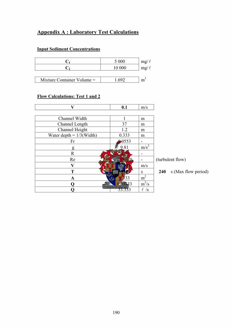
190

Appendix A : Laboratory Test Calculations Input Sediment Concentrations

C1 5 000 mg/ l C2 10 000 mg/ l

Mixture Container Volume = 1.692 m3

Flow Calculations: Test 1 and 2

V 0.1 m/s

Channel Width 1 m Channel Length 37 m Channel Height 1.2 m

Water depth = 1/3(Width) 0.333 m Fr 0.0553 - g 9.81 m/s2 R 0.20 - Re 20008.0 - (turbulent flow) V 0.100 m/s T 370 s 240 s (Max flow period) A 0.333 m2 Q 0.03333 m3/s Q 33.333 l /s

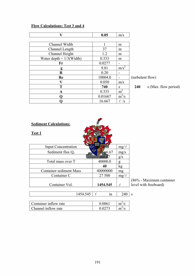
191

Flow Calculations: Test 3 and 4

V 0.05 m/s

Channel Width 1 m Channel Length 37 m Channel Height 1.2 m

Water depth = 1/3(Width) 0.333 m Fr 0.0277 - g 9.81 m/s2 R 0.20 - Re 10004.0 - (turbulent flow) V 0.050 m/s T 740 s 240 s (Max. flow period) A 0.333 m2 Q 0.01667 m3/s Q 16.667 l /s

Sediment Calculations:

Test 1

Input Concentration 5 000 mg/ l Sediment flux Qs 166666.67 mg/s

166.67 g/s Total mass over T 40000.0 g

40 kg Container sediment Mass 40000000 mg

Container C 27 500 mg/ l

Container Vol. 1454.545 l (86% - Maximum container level with freeboard)

1454.545 l in 240 s

Container inflow rate 0.0061 m3/s Channel inflow rate 0.0273 m3/s

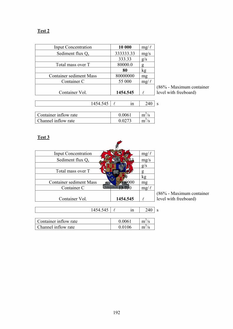
192

Test 2

Input Concentration 10 000 mg/ l Sediment flux Qs 333333.33 mg/s

333.33 g/s Total mass over T 80000.0 g

80 kg Container sediment Mass 80000000 mg

Container C 55 000 mg/ l

Container Vol. 1454.545 l (86% - Maximum container level with freeboard)

1454.545 l in 240 s

Container inflow rate 0.0061 m3/s Channel inflow rate 0.0273 m3/s Test 3

Input Concentration 5 000 mg/ l Sediment flux Qs 83333.33 mg/s

83.33 g/s Total mass over T 20000.0 g

20 kg Container sediment Mass 20000000 mg

Container C 13 750 mg/ l

Container Vol. 1454.545 l (86% - Maximum container level with freeboard)

1454.545 l in 240 s

Container inflow rate 0.0061 m3/s Channel inflow rate 0.0106 m3/s

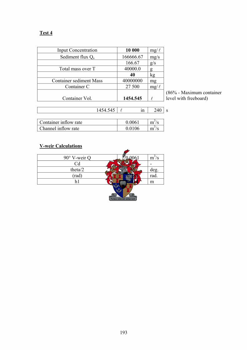
193

Test 4

Input Concentration 10 000 mg/ l Sediment flux Qs 166666.67 mg/s

166.67 g/s Total mass over T 40000.0 g

40 kg Container sediment Mass 40000000 mg

Container C 27 500 mg/ l

Container Vol. 1454.545 l (86% - Maximum container level with freeboard)

1454.545 l in 240 s

Container inflow rate 0.0061 m3/s Channel inflow rate 0.0106 m3/s V-weir Calculations

90° V-weir Q 0.0061 m3/s Cd 0.59 -

theta/2 45 deg. (rad) 0.785 rad. h1 0.114 m

194

Appendix B : ASTM Method for Determining Particle Size Distribution Sediment used in laboratory experiments: Western Province Ball Clay (a very fine light brown powder) A sieve analysis showed that all the particles were smaller than 0.075mm (75μm), thus the ASTM hydrometer method was used to determine the size distribution of the particles In this method a 60g (w) sample of particles smaller than 2.36mm is mixed into 120ml of sodium hexametaphosphate solution (40g/ l ) and left for 16 hours. Afterwards it is poured into a 1000ml sedimentation cylinder which is then filled up with distilled water and placed in a constant temperature bath until the suspension reaches 20°C. The cylinder is then taken out of the bath and turned upside down and back for 60 seconds, and placed back in the bath. Readings are taken with an ASTM 152H hydrometer at increasing time intervals. The temperature of the suspension is also measured after every reading. Hydrometer Readings Time (min) Reading *Corrected reading Temp (°C) 2 57.5 52.5 20 5 56 51 20 15 54 49 19.7 30 52.5 47.5 19.7 60 51 46 19.5 250 49 44 21 1440 45.5 40.5 19.5 * The correction is made to bring the density of the sodium hexametaphosphate and distilled water solution into account. (subtracting it's hydrometer reading of 5)

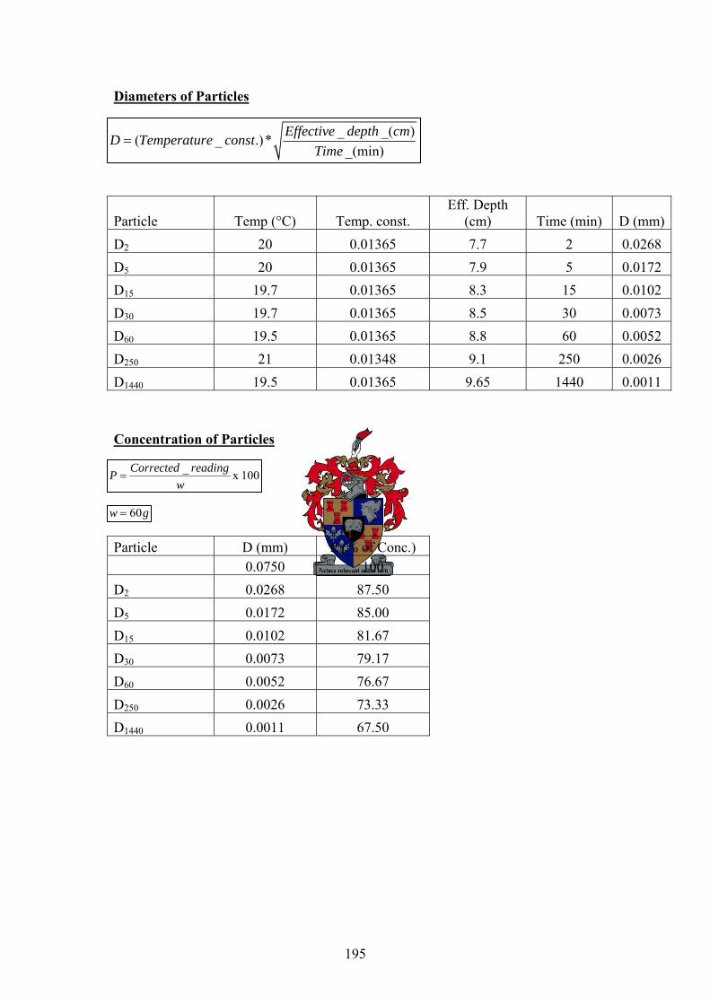
195

Diameters of Particles

Particle Temp (°C) Temp. const. Eff. Depth

(cm) Time (min) D (mm) D2 20 0.01365 7.7 2 0.0268 D5 20 0.01365 7.9 5 0.0172 D15 19.7 0.01365 8.3 15 0.0102 D30 19.7 0.01365 8.5 30 0.0073 D60 19.5 0.01365 8.8 60 0.0052 D250 21 0.01348 9.1 250 0.0026 D1440 19.5 0.01365 9.65 1440 0.0011 Concentration of Particles Particle D (mm) P (% of Conc.) 0.0750 100

D2 0.0268 87.50

D5 0.0172 85.00

D15 0.0102 81.67

D30 0.0073 79.17

D60 0.0052 76.67

D250 0.0026 73.33

D1440 0.0011 67.50

_ x 100Corrected readingPw

=

60w g=

_ _( )( _ .)*_(min)

Effective depth cmD Temperature constTime

=

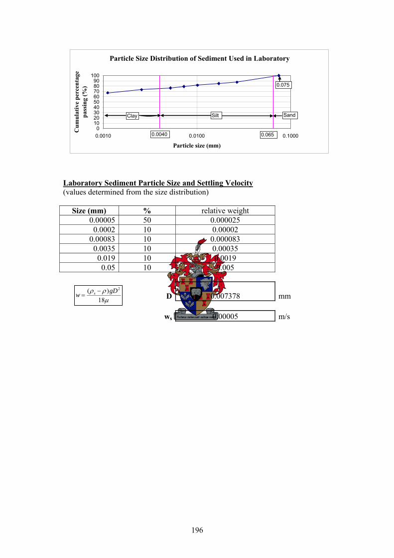
196

Particle Size Distribution of Sediment Used in Laboratory

0102030405060708090

100

0.0010 0.0100 0.1000

Particle size (mm)

Cum

ulat

ive

perc

enta

ge

pass

ing

(%)

SiltClay

0.0040

Sand

0.065

0.075

Laboratory Sediment Particle Size and Settling Velocity (values determined from the size distribution)

Size (mm) % relative weight 0.00005 50 0.000025 0.0002 10 0.00002

0.00083 10 0.000083 0.0035 10 0.00035 0.019 10 0.0019 0.05 10 0.005

D 0.007378 mm ws 0.00005 m/s

2( )18

s gDw ρ ρμ

−=

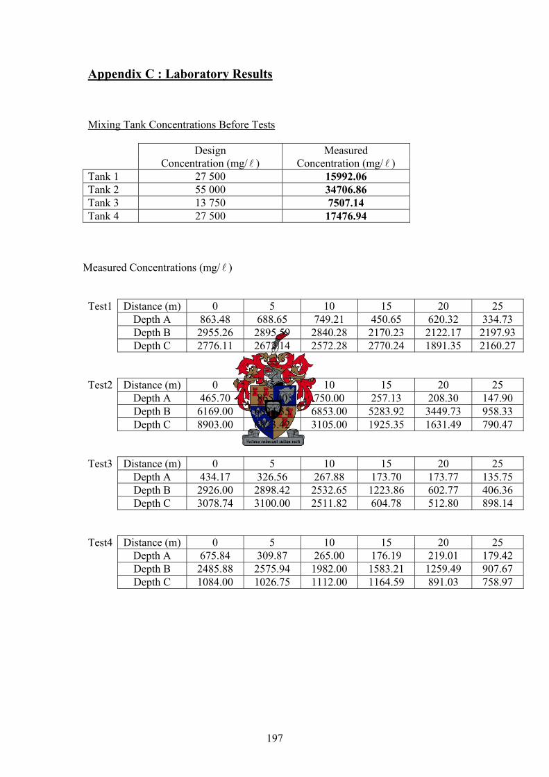
197

Appendix C : Laboratory Results Mixing Tank Concentrations Before Tests Design Measured Concentration (mg/ l ) Concentration (mg/ l ) Tank 1 27 500 15992.06 Tank 2 55 000 34706.86 Tank 3 13 750 7507.14 Tank 4 27 500 17476.94

Measured Concentrations (mg/ l )

Test1 Distance (m) 0 5 10 15 20 25

Depth A 863.48 688.65 749.21 450.65 620.32 334.73 Depth B 2955.26 2895.59 2840.28 2170.23 2122.17 2197.93 Depth C 2776.11 2672.14 2572.28 2770.24 1891.35 2160.27

Test2 Distance (m) 0 5 10 15 20 25

Depth A 465.70 865.00 750.00 257.13 208.30 147.90 Depth B 6169.00 6824.35 6853.00 5283.92 3449.73 958.33 Depth C 8903.00 6823.42 3105.00 1925.35 1631.49 790.47

Test3 Distance (m) 0 5 10 15 20 25 Depth A 434.17 326.56 267.88 173.70 173.77 135.75 Depth B 2926.00 2898.42 2532.65 1223.86 602.77 406.36 Depth C 3078.74 3100.00 2511.82 604.78 512.80 898.14

Test4 Distance (m) 0 5 10 15 20 25

Depth A 675.84 309.87 265.00 176.19 219.01 179.42 Depth B 2485.88 2575.94 1982.00 1583.21 1259.49 907.67 Depth C 1084.00 1026.75 1112.00 1164.59 891.03 758.97

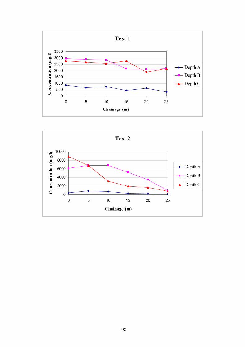
198

Test 1

0500

100015002000250030003500

0 5 10 15 20 25

Chainage (m)

Con

cent

ratio

n (m

g/l)

Depth ADepth B

Depth C

Test 2

0

2000

4000

6000

8000

10000

0 5 10 15 20 25

Chainage (m)

Con

cent

ratio

n (m

g/l)

Depth A

Depth B

Depth C

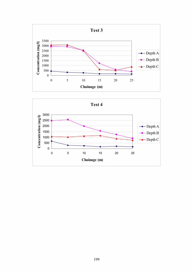
199

Test 3

0500

100015002000250030003500

0 5 10 15 20 25

Chainage (m)

Con

cent

ratio

n (m

g/l)

Depth A

Depth B

Depth C

Test 4

0

500

1000

1500

2000

2500

3000

0 5 10 15 20 25

Chainage (m)

Con

cent

ratio

n (m

g/l)

Depth A

Depth B

Depth C

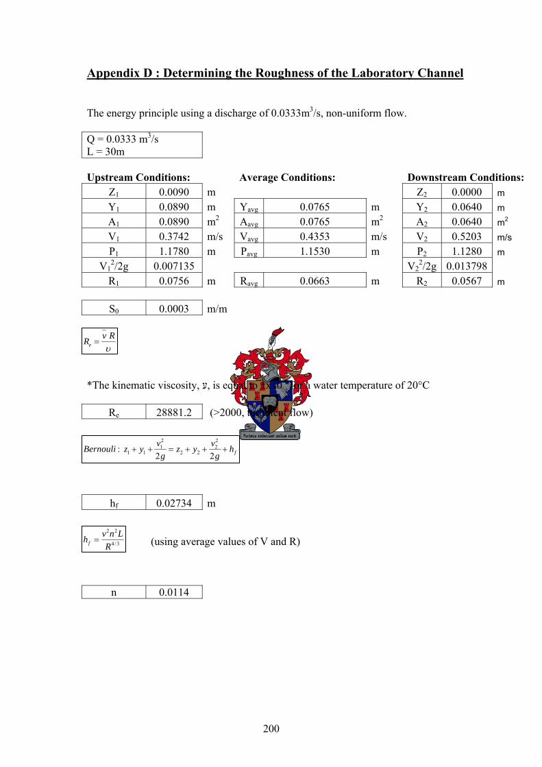
200

Appendix D : Determining the Roughness of the Laboratory Channel The energy principle using a discharge of 0.0333m3/s, non-uniform flow. Q = 0.0333 m3/s L = 30m Upstream Conditions: Average Conditions: Downstream Conditions:

Z1 0.0090 m Z2 0.0000 m Y1 0.0890 m Yavg 0.0765 m Y2 0.0640 m A1 0.0890 m2 Aavg 0.0765 m2 A2 0.0640 m2 V1 0.3742 m/s Vavg 0.4353 m/s V2 0.5203 m/s P1 1.1780 m Pavg 1.1530 m P2 1.1280 m

V12/2g 0.007135 V2

2/2g 0.013798 R1 0.0756 m Ravg 0.0663 m R2 0.0567 m

S0 0.0003 m/m

*The kinematic viscosity, ע, is equal to 1x10-6 for a water temperature of 20°C

Re 28881.2 (>2000, turbulent flow)

hf 0.02734 m (using average values of V and R)

n 0.0114

2 21 2

1 1 2 2: 2 2 fv vBernouli z y z y hg g

+ + = + + +

e

v RRυ

=

2 2

4/3fv n LhR

=

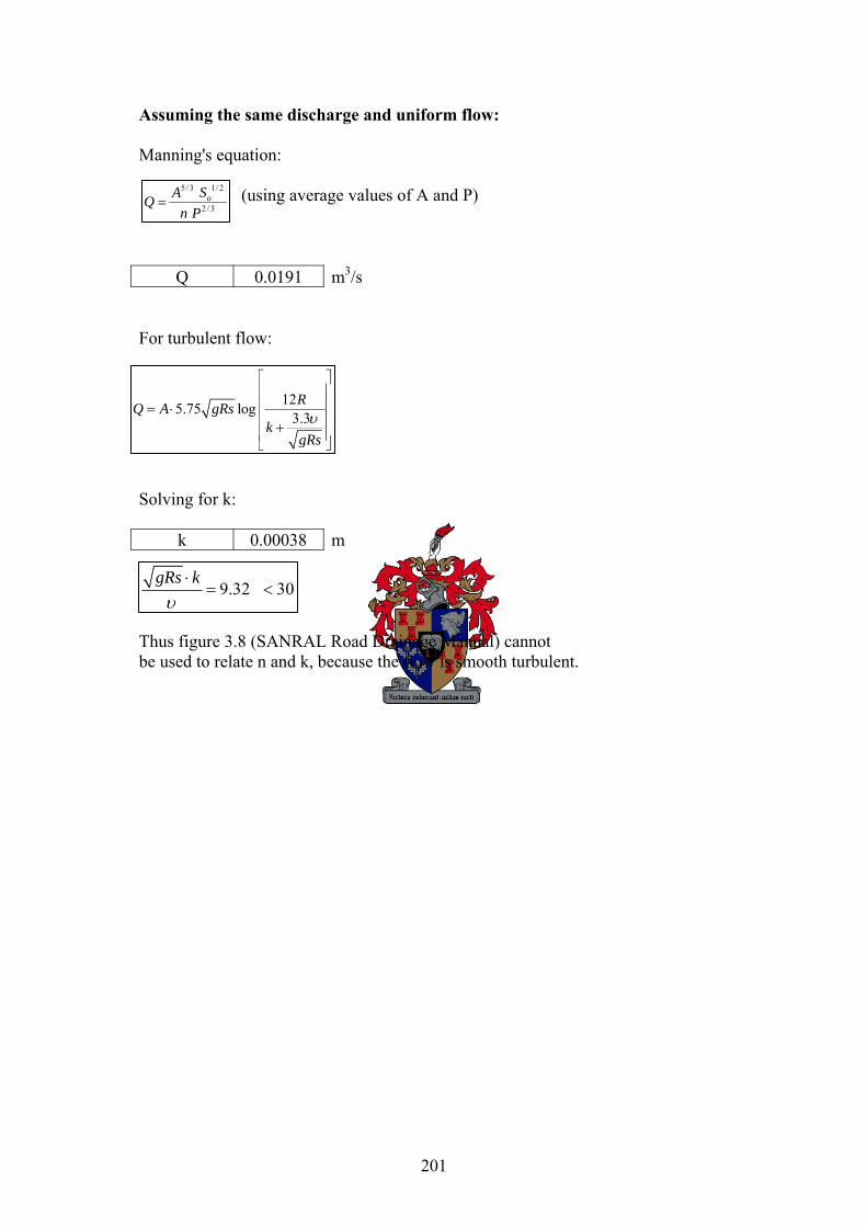
201

Assuming the same discharge and uniform flow: Manning's equation: (using average values of A and P)

Q 0.0191 m3/s For turbulent flow: Solving for k:

k 0.00038 m Thus figure 3.8 (SANRAL Road Drainage Manual) cannot be used to relate n and k, because the flow is smooth turbulent.

5/3 1/ 2

2 / 3

oA SQn P

=

125.75 log 3.3RQ A gRs

kgRsυ

⎡ ⎤⎢ ⎥⎢ ⎥= ⋅⎢ ⎥+⎢ ⎥⎣ ⎦

9.32 30gRs kυ

⋅= <

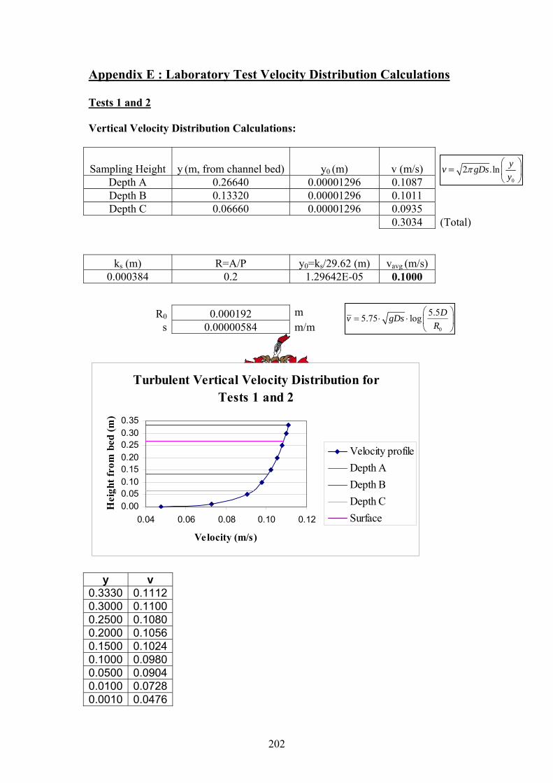
202

Appendix E : Laboratory Test Velocity Distribution Calculations Tests 1 and 2 Vertical Velocity Distribution Calculations:

Sampling Height y (m, from channel bed) y0 (m) v (m/s)

Depth A 0.26640 0.00001296 0.1087 Depth B 0.13320 0.00001296 0.1011 Depth C 0.06660 0.00001296 0.0935

0.3034 (Total)

ks (m) R=A/P y0=ks/29.62 (m) vavg (m/s) 0.000384 0.2 1.29642E-05 0.1000

R0 0.000192 m

s 0.00000584 m/m

Turbulent Vertical Velocity Distribution for Tests 1 and 2

0.000.050.100.150.200.250.300.35

0.04 0.06 0.08 0.10 0.12

Velocity (m/s)

Hei

ght f

rom

bed

(m)

Velocity profileDepth ADepth BDepth CSurface

y v 0.3330 0.11120.3000 0.11000.2500 0.10800.2000 0.10560.1500 0.10240.1000 0.09800.0500 0.09040.0100 0.07280.0010 0.0476

0

2 .ln ygDsy

v π⎛ ⎞⎜ ⎟⎝ ⎠

=

0

5.55.75 log Dv gDsR

⎛ ⎞= ⋅ ⋅ ⎜ ⎟

⎝ ⎠

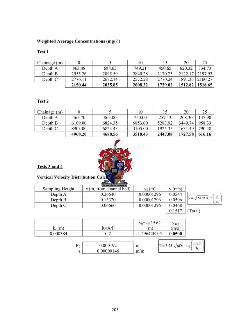
203

Weighted Average Concentrations (mg/ l ) Test 1 Chainage (m) 0 5 10 15 20 25

Depth A 863.48 688.65 749.21 450.65 620.32 334.73 Depth B 2955.26 2895.59 2840.28 2170.23 2122.17 2197.93Depth C 2776.11 2672.14 2572.28 2770.24 1891.35 2160.27

2150.44 2035.85 2008.32 1739.02 1512.82 1518.65 Test 2

Chainage (m) 0 5 10 15 20 25

Depth A 465.70 865.00 750.00 257.13 208.30 147.90 Depth B 6169.00 6824.35 6853.00 5283.92 3449.74 958.33 Depth C 8903.00 6823.43 3105.00 1925.35 1631.49 790.48

4968.20 4688.56 3510.43 2447.08 1727.58 616.16

Tests 3 and 4 Vertical Velocity Distribution Calculations:

Sampling Height y (m, from channel bed) y0 (m) v (m/s) Depth A 0.26640 0.00001296 0.0544 Depth B 0.13320 0.00001296 0.0506

Depth C 0.06660 0.00001296 0.0468 0.1517 (Total)

ks (m) R=A/P y0=ks/29.62

(m) vavg

(m/s)

0.000384 0.2 1.29642E-05 0.0500

R0 0.000192 m

s 0.00000146 m/m

0

2 .ln ygDsy

v π⎛ ⎞⎜ ⎟⎝ ⎠

=

0

5.55.75 log Dv gDsR

⎛ ⎞= ⋅ ⋅ ⎜ ⎟

⎝ ⎠

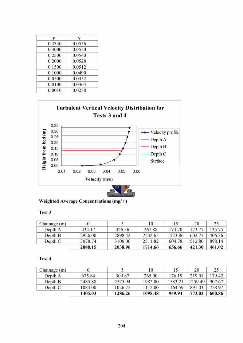
204

y v

0.3330 0.0556 0.3000 0.0550 0.2500 0.0540 0.2000 0.0528 0.1500 0.0512 0.1000 0.0490 0.0500 0.0452 0.0100 0.0364 0.0010 0.0238

Turbulent Vertical Velocity Distribution for Tests 3 and 4

0.000.050.100.150.200.250.300.35

0.01 0.02 0.03 0.04 0.05 0.06

Velocity (m/s)

Hei

ght f

rom

bed

(m)

Velocity profileDepth ADepth BDepth CSurface

Weighted Average Concentrations (mg/ l ) Test 3

Chainage (m) 0 5 10 15 20 25

Depth A 434.17 326.56 267.88 173.70 173.77 135.75 Depth B 2926.00 2898.42 2532.65 1223.86 602.77 406.36 Depth C 3078.74 3100.00 2511.82 604.78 512.80 898.14

2080.15 2038.96 1714.66 656.66 421.30 461.02 Test 4 Chainage (m) 0 5 10 15 20 25

Depth A 675.84 309.87 265.00 176.19 219.01 179.42 Depth B 2485.88 2575.94 1982.00 1583.21 1259.49 907.67 Depth C 1084.00 1026.75 1112.00 1164.59 891.03 758.97

1405.03 1286.26 1098.48 949.94 773.03 600.86

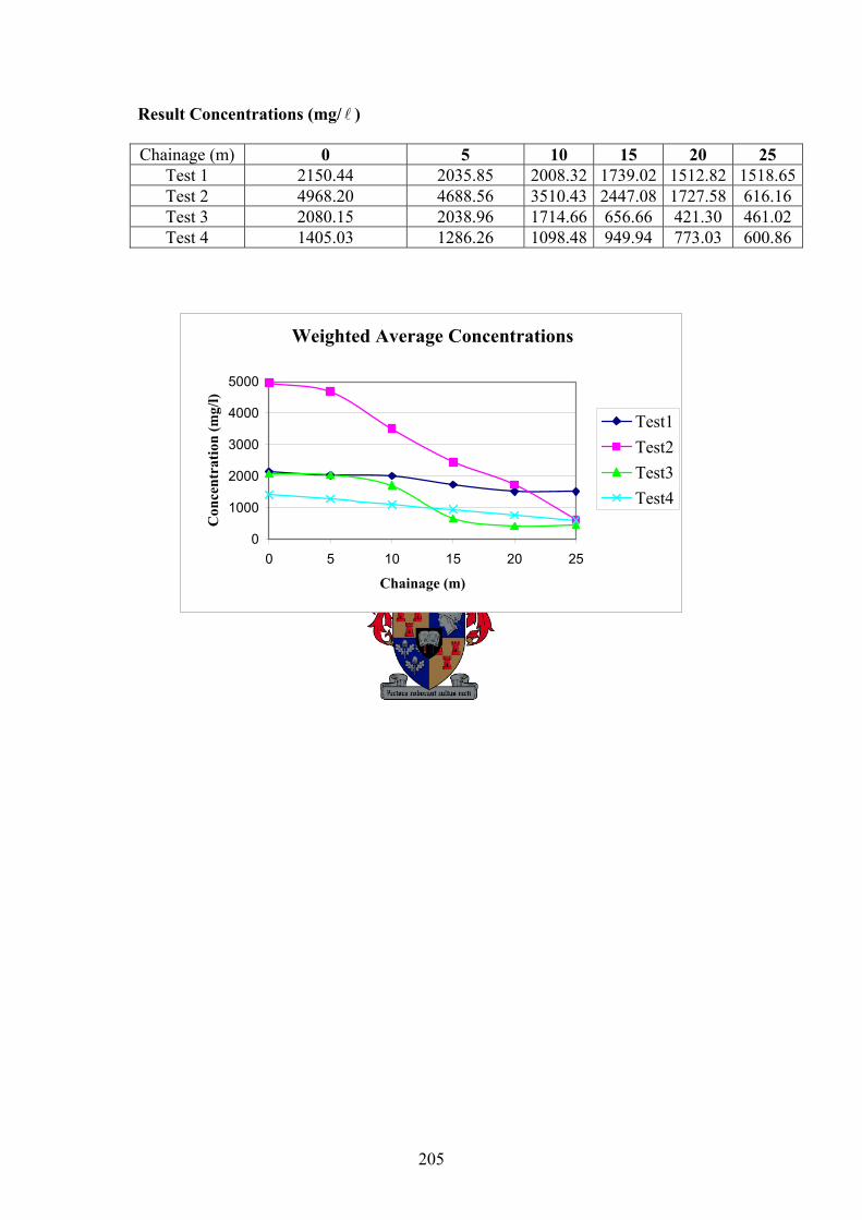
205

Result Concentrations (mg/ l )

Chainage (m) 0 5 10 15 20 25 Test 1 2150.44 2035.85 2008.32 1739.02 1512.82 1518.65Test 2 4968.20 4688.56 3510.43 2447.08 1727.58 616.16 Test 3 2080.15 2038.96 1714.66 656.66 421.30 461.02 Test 4 1405.03 1286.26 1098.48 949.94 773.03 600.86

Weighted Average Concentrations

0

1000

2000

3000

4000

5000

0 5 10 15 20 25

Chainage (m)

Con

cent

ratio

n (m

g/l)

Test1Test2Test3Test4

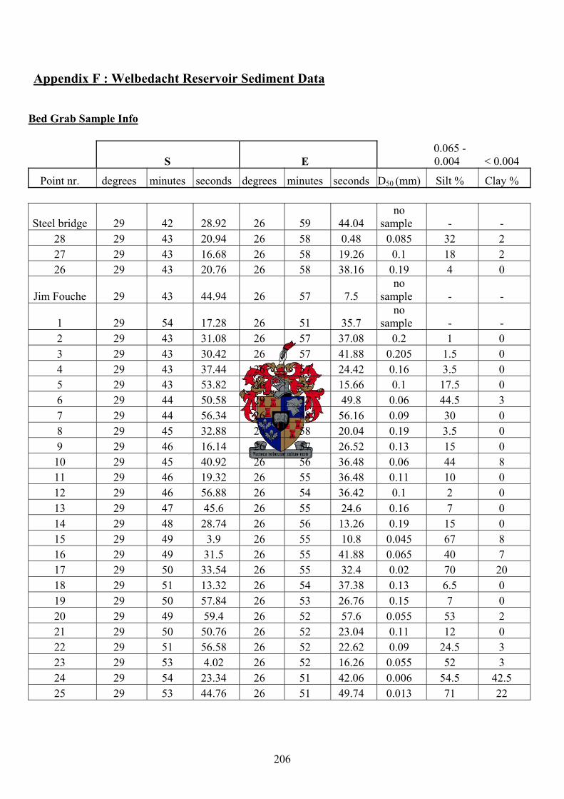
206

Appendix F : Welbedacht Reservoir Sediment Data Bed Grab Sample Info

S E 0.065 - 0.004 < 0.004

Point nr. degrees minutes seconds degrees minutes seconds D50 (mm) Silt % Clay %

Steel bridge 29 42 28.92 26 59 44.04 no

sample - - 28 29 43 20.94 26 58 0.48 0.085 32 2 27 29 43 16.68 26 58 19.26 0.1 18 2 26 29 43 20.76 26 58 38.16 0.19 4 0

Jim Fouche 29 43 44.94 26 57 7.5 no

sample - -

1 29 54 17.28 26 51 35.7 no

sample - - 2 29 43 31.08 26 57 37.08 0.2 1 0 3 29 43 30.42 26 57 41.88 0.205 1.5 0 4 29 43 37.44 26 57 24.42 0.16 3.5 0 5 29 43 53.82 26 57 15.66 0.1 17.5 0 6 29 44 50.58 29 57 49.8 0.06 44.5 3 7 29 44 56.34 26 58 56.16 0.09 30 0 8 29 45 32.88 26 58 20.04 0.19 3.5 0 9 29 46 16.14 26 57 26.52 0.13 15 0 10 29 45 40.92 26 56 36.48 0.06 44 8 11 29 46 19.32 26 55 36.48 0.11 10 0 12 29 46 56.88 26 54 36.42 0.1 2 0 13 29 47 45.6 26 55 24.6 0.16 7 0 14 29 48 28.74 26 56 13.26 0.19 15 0 15 29 49 3.9 26 55 10.8 0.045 67 8 16 29 49 31.5 26 55 41.88 0.065 40 7 17 29 50 33.54 26 55 32.4 0.02 70 20 18 29 51 13.32 26 54 37.38 0.13 6.5 0 19 29 50 57.84 26 53 26.76 0.15 7 0 20 29 49 59.4 26 52 57.6 0.055 53 2 21 29 50 50.76 26 52 23.04 0.11 12 0 22 29 51 56.58 26 52 22.62 0.09 24.5 3 23 29 53 4.02 26 52 16.26 0.055 52 3 24 29 54 23.34 26 51 42.06 0.006 54.5 42.5 25 29 53 44.76 26 51 49.74 0.013 71 22

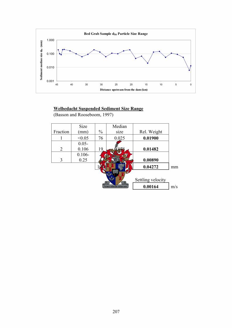
207

Bed Grab Sample d50 Particle Size Range

0.001

0.010

0.100

1.000

051015202530354045

Distance upstream from the dam (km)

Sedi

men

t med

ian

size

d 50

(mm

)

Welbedacht Suspended Sediment Size Range (Basson and Rooseboom, 1997)

FractionSize (mm) %

Median size Rel. Weight

1 <0.05 76 0.025 0.01900

2 0.05-0.106 19 0.078 0.01482

3 0.106-0.25 5 0.178 0.00890

100 0.04272 mm Settling velocity 0.00164 m/s

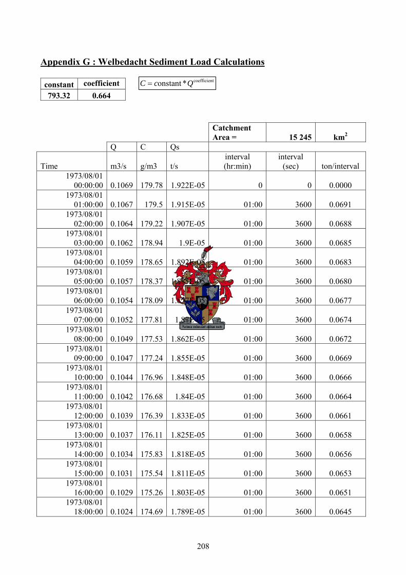
208

Appendix G : Welbedacht Sediment Load Calculations constant coefficient 793.32 0.664

Catchment Area = 15 245 km2

Q C Qs

Time m3/s g/m3 t/s interval (hr:min)

interval (sec) ton/interval

1973/08/01 00:00:00 0.1069 179.78 1.922E-05 0 0 0.0000

1973/08/01 01:00:00 0.1067 179.5 1.915E-05 01:00 3600 0.0691

1973/08/01 02:00:00 0.1064 179.22 1.907E-05 01:00 3600 0.0688

1973/08/01 03:00:00 0.1062 178.94 1.9E-05 01:00 3600 0.0685

1973/08/01 04:00:00 0.1059 178.65 1.892E-05 01:00 3600 0.0683

1973/08/01 05:00:00 0.1057 178.37 1.885E-05 01:00 3600 0.0680

1973/08/01 06:00:00 0.1054 178.09 1.877E-05 01:00 3600 0.0677

1973/08/01 07:00:00 0.1052 177.81 1.87E-05 01:00 3600 0.0674

1973/08/01 08:00:00 0.1049 177.53 1.862E-05 01:00 3600 0.0672

1973/08/01 09:00:00 0.1047 177.24 1.855E-05 01:00 3600 0.0669

1973/08/01 10:00:00 0.1044 176.96 1.848E-05 01:00 3600 0.0666

1973/08/01 11:00:00 0.1042 176.68 1.84E-05 01:00 3600 0.0664

1973/08/01 12:00:00 0.1039 176.39 1.833E-05 01:00 3600 0.0661

1973/08/01 13:00:00 0.1037 176.11 1.825E-05 01:00 3600 0.0658

1973/08/01 14:00:00 0.1034 175.83 1.818E-05 01:00 3600 0.0656

1973/08/01 15:00:00 0.1031 175.54 1.811E-05 01:00 3600 0.0653

1973/08/01 16:00:00 0.1029 175.26 1.803E-05 01:00 3600 0.0651

1973/08/01 18:00:00 0.1024 174.69 1.789E-05 01:00 3600 0.0645

coefficientonstant *C c Q=

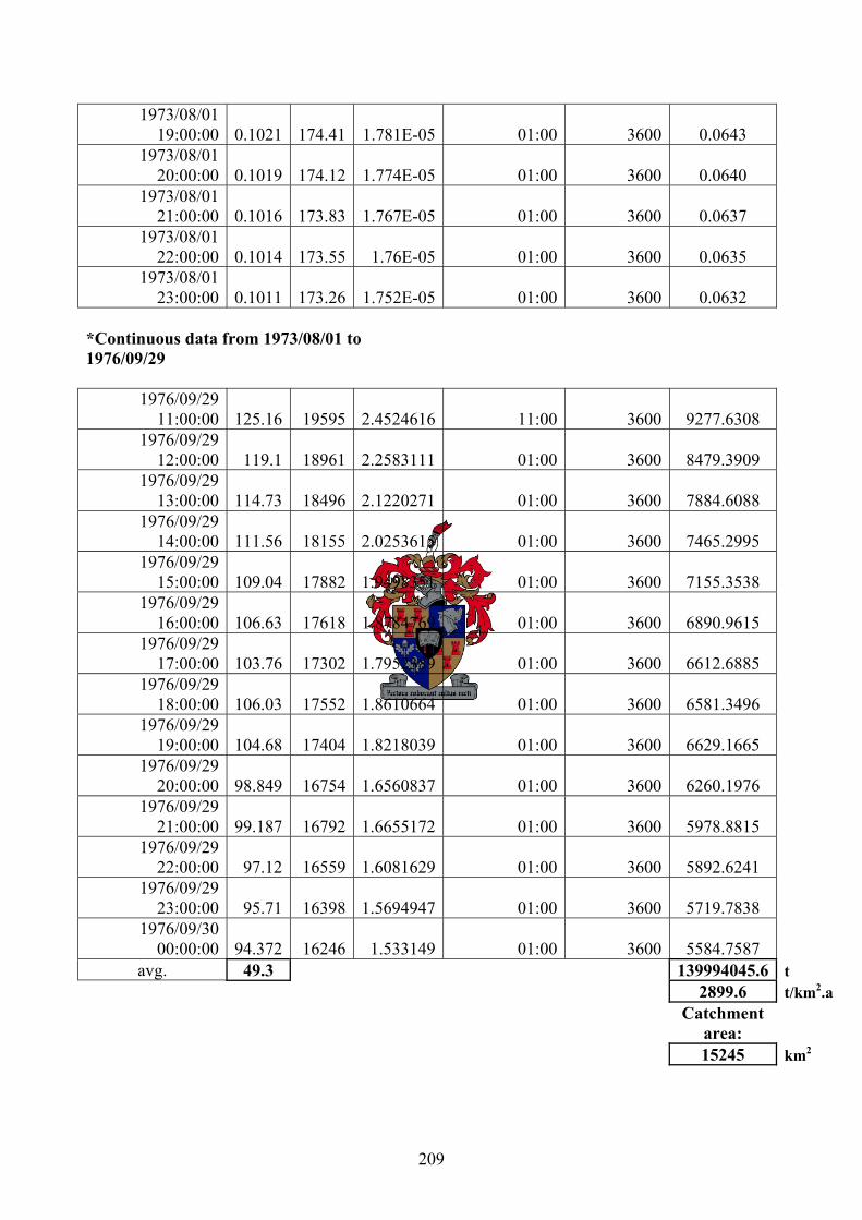
209

1973/08/01 19:00:00 0.1021 174.41 1.781E-05 01:00 3600 0.0643

1973/08/01 20:00:00 0.1019 174.12 1.774E-05 01:00 3600 0.0640

1973/08/01 21:00:00 0.1016 173.83 1.767E-05 01:00 3600 0.0637

1973/08/01 22:00:00 0.1014 173.55 1.76E-05 01:00 3600 0.0635

1973/08/01 23:00:00 0.1011 173.26 1.752E-05 01:00 3600 0.0632

*Continuous data from 1973/08/01 to 1976/09/29

1976/09/29 11:00:00 125.16 19595 2.4524616 11:00 3600 9277.6308

1976/09/29 12:00:00 119.1 18961 2.2583111 01:00 3600 8479.3909

1976/09/29 13:00:00 114.73 18496 2.1220271 01:00 3600 7884.6088

1976/09/29 14:00:00 111.56 18155 2.0253615 01:00 3600 7465.2995

1976/09/29 15:00:00 109.04 17882 1.9498351 01:00 3600 7155.3538

1976/09/29 16:00:00 106.63 17618 1.8784769 01:00 3600 6890.9615

1976/09/29 17:00:00 103.76 17302 1.7952389 01:00 3600 6612.6885

1976/09/29 18:00:00 106.03 17552 1.8610664 01:00 3600 6581.3496

1976/09/29 19:00:00 104.68 17404 1.8218039 01:00 3600 6629.1665

1976/09/29 20:00:00 98.849 16754 1.6560837 01:00 3600 6260.1976

1976/09/29 21:00:00 99.187 16792 1.6655172 01:00 3600 5978.8815

1976/09/29 22:00:00 97.12 16559 1.6081629 01:00 3600 5892.6241

1976/09/29 23:00:00 95.71 16398 1.5694947 01:00 3600 5719.7838

1976/09/30 00:00:00 94.372 16246 1.533149 01:00 3600 5584.7587

avg. 49.3 139994045.6 t 2899.6 t/km2.a

Catchment

area: 15245 km2

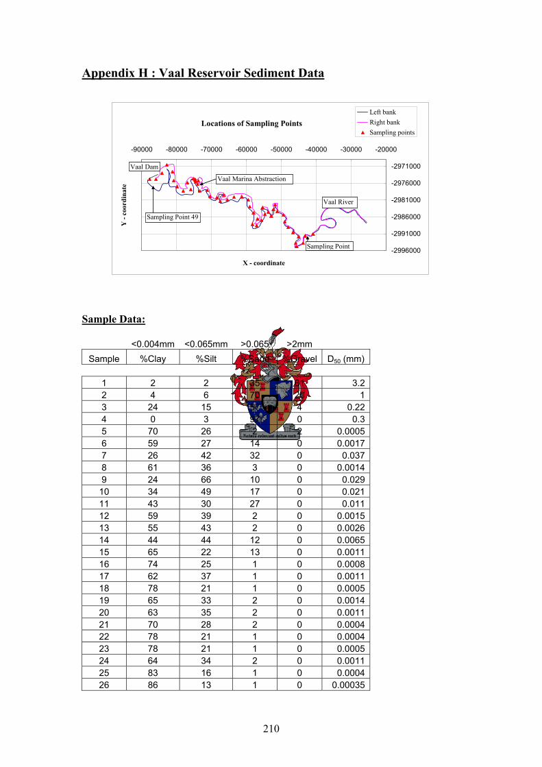
210

Appendix H : Vaal Reservoir Sediment Data

Locations of Sampling Points

-2996000

-2991000

-2986000

-2981000

-2976000

-2971000

-90000 -80000 -70000 -60000 -50000 -40000 -30000 -20000

X - coordinate

Y -

coor

dina

te

Left bankRight bankSampling points

Sampling Point 49

Sampling Point

Vaal Dam

Vaal Marina Abstraction

Vaal River

Sample Data:

<0.004mm <0.065mm >0.065 >2mm Sample %Clay %Silt %Sand %Gravel D50 (mm)

1 2 2 35 61 3.2 2 4 6 70 20 1 3 24 15 57 4 0.22 4 0 3 97 0 0.3 5 70 26 2 2 0.0005 6 59 27 14 0 0.0017 7 26 42 32 0 0.037 8 61 36 3 0 0.0014 9 24 66 10 0 0.029

10 34 49 17 0 0.021 11 43 30 27 0 0.011 12 59 39 2 0 0.0015 13 55 43 2 0 0.0026 14 44 44 12 0 0.0065 15 65 22 13 0 0.0011 16 74 25 1 0 0.0008 17 62 37 1 0 0.0011 18 78 21 1 0 0.0005 19 65 33 2 0 0.0014 20 63 35 2 0 0.0011 21 70 28 2 0 0.0004 22 78 21 1 0 0.0004 23 78 21 1 0 0.0005 24 64 34 2 0 0.0011 25 83 16 1 0 0.0004 26 86 13 1 0 0.00035

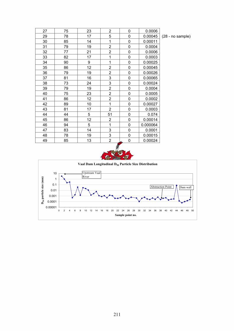
211

27 75 23 2 0 0.0006 29 78 17 5 0 0.00045 (28 - no sample) 30 85 14 1 0 0.00011 31 79 19 2 0 0.0004 32 77 21 2 0 0.0006 33 82 17 1 0 0.0003 34 90 9 1 0 0.00025 35 86 12 2 0 0.00045 36 79 19 2 0 0.00026 37 81 16 3 0 0.00065 38 73 24 3 0 0.00024 39 79 19 2 0 0.0004 40 75 23 2 0 0.0005 41 86 12 2 0 0.0002 42 89 10 1 0 0.00027 43 81 17 2 0 0.0003 44 44 5 51 0 0.074 45 86 12 2 0 0.00014 46 94 5 1 0 0.000064 47 83 14 3 0 0.0001 48 78 19 3 0 0.00015 49 85 13 2 0 0.00024

Vaal Dam Longitudinal D50 Particle Size Distribution

0.00001

0.0001

0.001

0.01

0.1

1

10

0 2 4 6 8 10 12 14 16 18 20 22 24 26 28 30 32 34 36 38 40 42 44 46 48 50

Sample point no.

D50

par

ticle

size

(mm

)

Abstraction Point

Upstream Vaal River

Dam wall

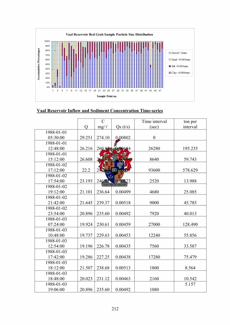
212

Vaal Reservoir Bed Grab Sample Particle Size Distribution

0%

10%

20%

30%

40%

50%

60%

70%

80%

90%

100%

1 3 5 7 9 11 13 15 17 19 21 23 25 27 29 31 33 35 37 39 41 43 45 47

Sample Point no.

Acc

umul

ativ

e Pe

rcen

tage

s

Gravel >2mm

Sand >0.065mm

Silt <0.065mm

Clay <0.004mm

Vaal Reservoir Inflow and Sediment Concentration Time-series

Q C

mg/ l Qs (t/s) Time interval

(sec) ton per interval

1988-01-01 05:30:00 29.251 274.10 0.00802 0

1988-01-01 12:48:00 26.216 260.92 0.00684 26280 195.235

1988-01-01 15:12:00 26.608 262.67 0.00699 8640 59.743

1988-01-02 17:12:00 22.2 242.11 0.00537 93600 578.629

1988-01-02 17:54:00 23.193 246.92 0.00573 2520 13.988

1988-01-02 19:12:00 21.101 236.64 0.00499 4680 25.085

1988-01-02 21:42:00 21.645 239.37 0.00518 9000 45.785

1988-01-02 23:54:00 20.896 235.60 0.00492 7920 40.013

1988-01-03 07:24:00 19.924 230.61 0.00459 27000 128.490

1988-01-03 10:48:00 19.737 229.63 0.00453 12240 55.856

1988-01-03 12:54:00 19.196 226.78 0.00435 7560 33.587

1988-01-03 17:42:00 19.286 227.25 0.00438 17280 75.479

1988-01-03 18:12:00 21.507 238.68 0.00513 1800 8.564

1988-01-03 18:48:00 20.023 231.12 0.00463 2160 10.542

1988-01-03 19:06:00 20.896 235.60 0.00492 1080

5.157

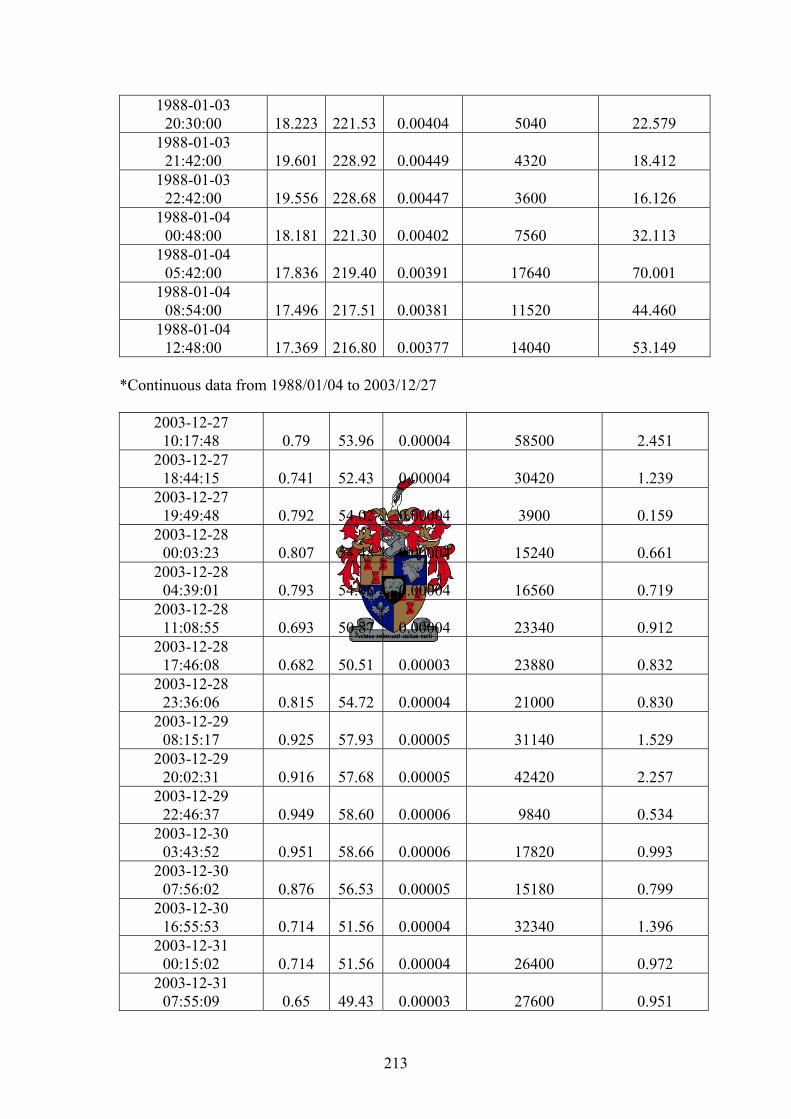
213

1988-01-03 20:30:00 18.223 221.53 0.00404 5040 22.579

1988-01-03 21:42:00 19.601 228.92 0.00449 4320 18.412

1988-01-03 22:42:00 19.556 228.68 0.00447 3600 16.126

1988-01-04 00:48:00 18.181 221.30 0.00402 7560 32.113

1988-01-04 05:42:00 17.836 219.40 0.00391 17640 70.001

1988-01-04 08:54:00 17.496 217.51 0.00381 11520 44.460

1988-01-04 12:48:00 17.369 216.80 0.00377 14040 53.149

*Continuous data from 1988/01/04 to 2003/12/27

2003-12-27 10:17:48 0.79 53.96 0.00004 58500 2.451

2003-12-27 18:44:15 0.741 52.43 0.00004 30420 1.239

2003-12-27 19:49:48 0.792 54.02 0.00004 3900 0.159

2003-12-28 00:03:23 0.807 54.48 0.00004 15240 0.661

2003-12-28 04:39:01 0.793 54.05 0.00004 16560 0.719

2003-12-28 11:08:55 0.693 50.87 0.00004 23340 0.912

2003-12-28 17:46:08 0.682 50.51 0.00003 23880 0.832

2003-12-28 23:36:06 0.815 54.72 0.00004 21000 0.830

2003-12-29 08:15:17 0.925 57.93 0.00005 31140 1.529

2003-12-29 20:02:31 0.916 57.68 0.00005 42420 2.257

2003-12-29 22:46:37 0.949 58.60 0.00006 9840 0.534

2003-12-30 03:43:52 0.951 58.66 0.00006 17820 0.993

2003-12-30 07:56:02 0.876 56.53 0.00005 15180 0.799

2003-12-30 16:55:53 0.714 51.56 0.00004 32340 1.396

2003-12-31 00:15:02 0.714 51.56 0.00004 26400 0.972

2003-12-31 07:55:09 0.65 49.43 0.00003 27600 0.951

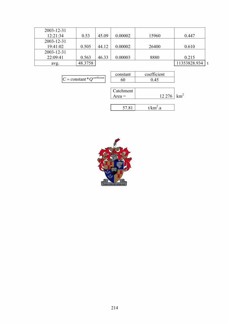
214

2003-12-31 12:21:34 0.53 45.09 0.00002 15960 0.447

2003-12-31 19:41:02 0.505 44.12 0.00002 26400 0.610

2003-12-31 22:09:41 0.563 46.33 0.00003 8880 0.215

avg. 48.3758 11353828.934 t constant coefficient 60 0.45

Catchment Area = 12 276 km2

57.81 t/km2.a

coefficientonstant *C c Q=

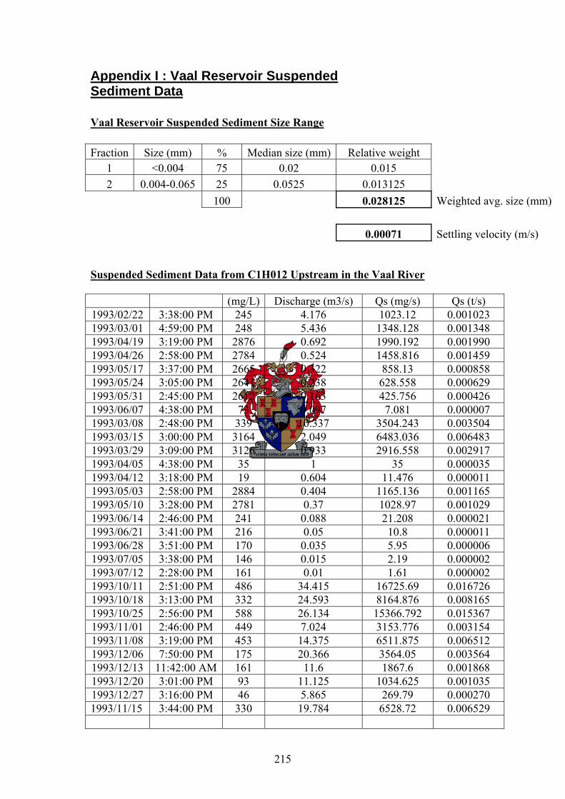
215

Appendix I : Vaal Reservoir Suspended Sediment Data Vaal Reservoir Suspended Sediment Size Range Fraction Size (mm) % Median size (mm) Relative weight

1 <0.004 75 0.02 0.015 2 0.004-0.065 25 0.0525 0.013125

100 0.028125 Weighted avg. size (mm) 0.00071 Settling velocity (m/s)

Suspended Sediment Data from C1H012 Upstream in the Vaal River

(mg/L) Discharge (m3/s) Qs (mg/s) Qs (t/s) 1993/02/22 3:38:00 PM 245 4.176 1023.12 0.001023 1993/03/01 4:59:00 PM 248 5.436 1348.128 0.001348 1993/04/19 3:19:00 PM 2876 0.692 1990.192 0.001990 1993/04/26 2:58:00 PM 2784 0.524 1458.816 0.001459 1993/05/17 3:37:00 PM 2665 0.322 858.13 0.000858 1993/05/24 3:05:00 PM 2641 0.238 628.558 0.000629 1993/05/31 2:45:00 PM 2612 0.163 425.756 0.000426 1993/06/07 4:38:00 PM 73 0.097 7.081 0.000007 1993/03/08 2:48:00 PM 339 10.337 3504.243 0.003504 1993/03/15 3:00:00 PM 3164 2.049 6483.036 0.006483 1993/03/29 3:09:00 PM 3126 0.933 2916.558 0.002917 1993/04/05 4:38:00 PM 35 1 35 0.000035 1993/04/12 3:18:00 PM 19 0.604 11.476 0.000011 1993/05/03 2:58:00 PM 2884 0.404 1165.136 0.001165 1993/05/10 3:28:00 PM 2781 0.37 1028.97 0.001029 1993/06/14 2:46:00 PM 241 0.088 21.208 0.000021 1993/06/21 3:41:00 PM 216 0.05 10.8 0.000011 1993/06/28 3:51:00 PM 170 0.035 5.95 0.000006 1993/07/05 3:38:00 PM 146 0.015 2.19 0.000002 1993/07/12 2:28:00 PM 161 0.01 1.61 0.000002 1993/10/11 2:51:00 PM 486 34.415 16725.69 0.016726 1993/10/18 3:13:00 PM 332 24.593 8164.876 0.008165 1993/10/25 2:56:00 PM 588 26.134 15366.792 0.015367 1993/11/01 2:46:00 PM 449 7.024 3153.776 0.003154 1993/11/08 3:19:00 PM 453 14.375 6511.875 0.006512 1993/12/06 7:50:00 PM 175 20.366 3564.05 0.003564 1993/12/13 11:42:00 AM 161 11.6 1867.6 0.001868 1993/12/20 3:01:00 PM 93 11.125 1034.625 0.001035 1993/12/27 3:16:00 PM 46 5.865 269.79 0.000270 1993/11/15 3:44:00 PM 330 19.784 6528.72 0.006529

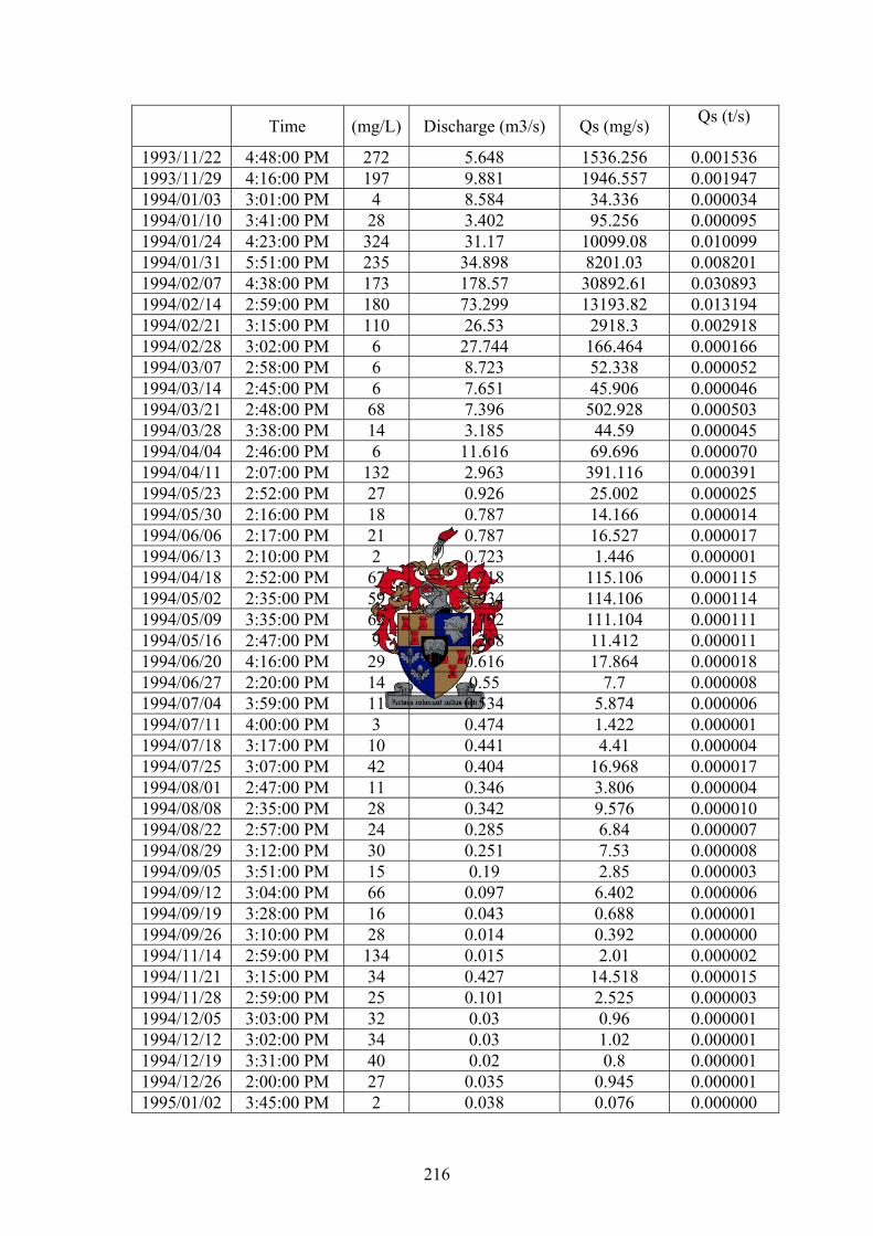
216

Time (mg/L) Discharge (m3/s) Qs (mg/s) Qs (t/s)

1993/11/22 4:48:00 PM 272 5.648 1536.256 0.001536 1993/11/29 4:16:00 PM 197 9.881 1946.557 0.001947 1994/01/03 3:01:00 PM 4 8.584 34.336 0.000034 1994/01/10 3:41:00 PM 28 3.402 95.256 0.000095 1994/01/24 4:23:00 PM 324 31.17 10099.08 0.010099 1994/01/31 5:51:00 PM 235 34.898 8201.03 0.008201 1994/02/07 4:38:00 PM 173 178.57 30892.61 0.030893 1994/02/14 2:59:00 PM 180 73.299 13193.82 0.013194 1994/02/21 3:15:00 PM 110 26.53 2918.3 0.002918 1994/02/28 3:02:00 PM 6 27.744 166.464 0.000166 1994/03/07 2:58:00 PM 6 8.723 52.338 0.000052 1994/03/14 2:45:00 PM 6 7.651 45.906 0.000046 1994/03/21 2:48:00 PM 68 7.396 502.928 0.000503 1994/03/28 3:38:00 PM 14 3.185 44.59 0.000045 1994/04/04 2:46:00 PM 6 11.616 69.696 0.000070 1994/04/11 2:07:00 PM 132 2.963 391.116 0.000391 1994/05/23 2:52:00 PM 27 0.926 25.002 0.000025 1994/05/30 2:16:00 PM 18 0.787 14.166 0.000014 1994/06/06 2:17:00 PM 21 0.787 16.527 0.000017 1994/06/13 2:10:00 PM 2 0.723 1.446 0.000001 1994/04/18 2:52:00 PM 67 1.718 115.106 0.000115 1994/05/02 2:35:00 PM 59 1.934 114.106 0.000114 1994/05/09 3:35:00 PM 62 1.792 111.104 0.000111 1994/05/16 2:47:00 PM 9 1.268 11.412 0.000011 1994/06/20 4:16:00 PM 29 0.616 17.864 0.000018 1994/06/27 2:20:00 PM 14 0.55 7.7 0.000008 1994/07/04 3:59:00 PM 11 0.534 5.874 0.000006 1994/07/11 4:00:00 PM 3 0.474 1.422 0.000001 1994/07/18 3:17:00 PM 10 0.441 4.41 0.000004 1994/07/25 3:07:00 PM 42 0.404 16.968 0.000017 1994/08/01 2:47:00 PM 11 0.346 3.806 0.000004 1994/08/08 2:35:00 PM 28 0.342 9.576 0.000010 1994/08/22 2:57:00 PM 24 0.285 6.84 0.000007 1994/08/29 3:12:00 PM 30 0.251 7.53 0.000008 1994/09/05 3:51:00 PM 15 0.19 2.85 0.000003 1994/09/12 3:04:00 PM 66 0.097 6.402 0.000006 1994/09/19 3:28:00 PM 16 0.043 0.688 0.000001 1994/09/26 3:10:00 PM 28 0.014 0.392 0.000000 1994/11/14 2:59:00 PM 134 0.015 2.01 0.000002 1994/11/21 3:15:00 PM 34 0.427 14.518 0.000015 1994/11/28 2:59:00 PM 25 0.101 2.525 0.000003 1994/12/05 3:03:00 PM 32 0.03 0.96 0.000001 1994/12/12 3:02:00 PM 34 0.03 1.02 0.000001 1994/12/19 3:31:00 PM 40 0.02 0.8 0.000001 1994/12/26 2:00:00 PM 27 0.035 0.945 0.000001 1995/01/02 3:45:00 PM 2 0.038 0.076 0.000000

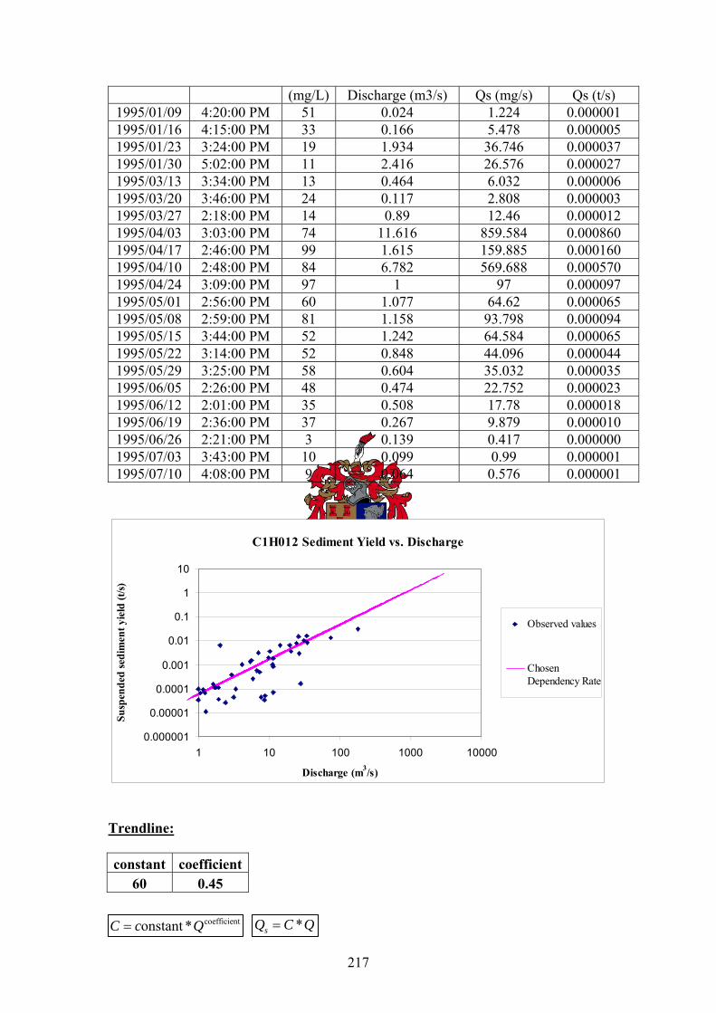
217

(mg/L) Discharge (m3/s) Qs (mg/s) Qs (t/s) 1995/01/09 4:20:00 PM 51 0.024 1.224 0.000001 1995/01/16 4:15:00 PM 33 0.166 5.478 0.000005 1995/01/23 3:24:00 PM 19 1.934 36.746 0.000037 1995/01/30 5:02:00 PM 11 2.416 26.576 0.000027 1995/03/13 3:34:00 PM 13 0.464 6.032 0.000006 1995/03/20 3:46:00 PM 24 0.117 2.808 0.000003 1995/03/27 2:18:00 PM 14 0.89 12.46 0.000012 1995/04/03 3:03:00 PM 74 11.616 859.584 0.000860 1995/04/17 2:46:00 PM 99 1.615 159.885 0.000160 1995/04/10 2:48:00 PM 84 6.782 569.688 0.000570 1995/04/24 3:09:00 PM 97 1 97 0.000097 1995/05/01 2:56:00 PM 60 1.077 64.62 0.000065 1995/05/08 2:59:00 PM 81 1.158 93.798 0.000094 1995/05/15 3:44:00 PM 52 1.242 64.584 0.000065 1995/05/22 3:14:00 PM 52 0.848 44.096 0.000044 1995/05/29 3:25:00 PM 58 0.604 35.032 0.000035 1995/06/05 2:26:00 PM 48 0.474 22.752 0.000023 1995/06/12 2:01:00 PM 35 0.508 17.78 0.000018 1995/06/19 2:36:00 PM 37 0.267 9.879 0.000010 1995/06/26 2:21:00 PM 3 0.139 0.417 0.000000 1995/07/03 3:43:00 PM 10 0.099 0.99 0.000001 1995/07/10 4:08:00 PM 9 0.064 0.576 0.000001

C1H012 Sediment Yield vs. Discharge

0.000001

0.00001

0.0001

0.001

0.01

0.1

1

10

1 10 100 1000 10000

Discharge (m3/s)

Susp

ende

d se

dim

ent y

ield

(t/s)

Observed values

ChosenDependency Rate

Trendline: constant coefficient

60 0.45 coefficientonstant *C c Q= *sQ C Q=

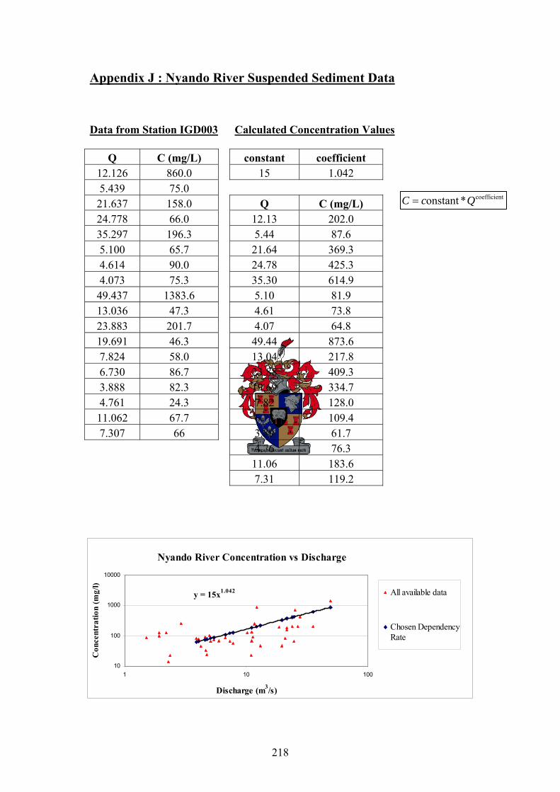
218

Appendix J : Nyando River Suspended Sediment Data Data from Station IGD003 Calculated Concentration Values

Q C (mg/L) constant coefficient 12.126 860.0 15 1.042 5.439 75.0 21.637 158.0 Q C (mg/L) 24.778 66.0 12.13 202.0 35.297 196.3 5.44 87.6 5.100 65.7 21.64 369.3 4.614 90.0 24.78 425.3 4.073 75.3 35.30 614.9 49.437 1383.6 5.10 81.9 13.036 47.3 4.61 73.8 23.883 201.7 4.07 64.8 19.691 46.3 49.44 873.6 7.824 58.0 13.04 217.8 6.730 86.7 23.88 409.3 3.888 82.3 19.69 334.7 4.761 24.3 7.82 128.0 11.062 67.7 6.73 109.4 7.307 66 3.89 61.7

4.76 76.3 11.06 183.6 7.31 119.2

Nyando River Concentration vs Discharge

y = 15x1.042

10

100

1000

10000

1 10 100

Discharge (m3/s)

Con

cent

ratio

n (m

g/l)

All available data

Chosen DependencyRate

coefficientonstant *C c Q=

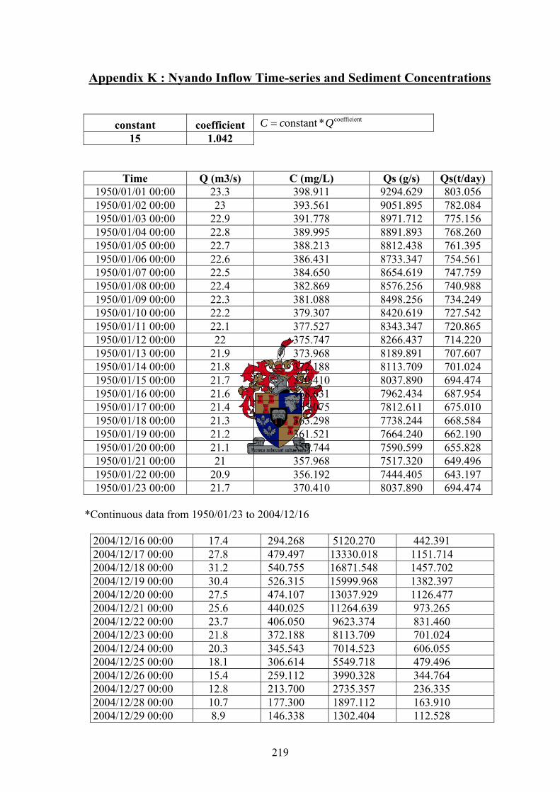
219

Appendix K : Nyando Inflow Time-series and Sediment Concentrations

constant coefficient coefficientonstant *C c Q= 15 1.042

Time Q (m3/s) C (mg/L) Qs (g/s) Qs(t/day) 1950/01/01 00:00 23.3 398.911 9294.629 803.056 1950/01/02 00:00 23 393.561 9051.895 782.084 1950/01/03 00:00 22.9 391.778 8971.712 775.156 1950/01/04 00:00 22.8 389.995 8891.893 768.260 1950/01/05 00:00 22.7 388.213 8812.438 761.395 1950/01/06 00:00 22.6 386.431 8733.347 754.561 1950/01/07 00:00 22.5 384.650 8654.619 747.759 1950/01/08 00:00 22.4 382.869 8576.256 740.988 1950/01/09 00:00 22.3 381.088 8498.256 734.249 1950/01/10 00:00 22.2 379.307 8420.619 727.542 1950/01/11 00:00 22.1 377.527 8343.347 720.865 1950/01/12 00:00 22 375.747 8266.437 714.220 1950/01/13 00:00 21.9 373.968 8189.891 707.607 1950/01/14 00:00 21.8 372.188 8113.709 701.024 1950/01/15 00:00 21.7 370.410 8037.890 694.474 1950/01/16 00:00 21.6 368.631 7962.434 687.954 1950/01/17 00:00 21.4 365.075 7812.611 675.010 1950/01/18 00:00 21.3 363.298 7738.244 668.584 1950/01/19 00:00 21.2 361.521 7664.240 662.190 1950/01/20 00:00 21.1 359.744 7590.599 655.828 1950/01/21 00:00 21 357.968 7517.320 649.496 1950/01/22 00:00 20.9 356.192 7444.405 643.197 1950/01/23 00:00 21.7 370.410 8037.890 694.474

*Continuous data from 1950/01/23 to 2004/12/16

2004/12/16 00:00 17.4 294.268 5120.270 442.391 2004/12/17 00:00 27.8 479.497 13330.018 1151.714 2004/12/18 00:00 31.2 540.755 16871.548 1457.702 2004/12/19 00:00 30.4 526.315 15999.968 1382.397 2004/12/20 00:00 27.5 474.107 13037.929 1126.477 2004/12/21 00:00 25.6 440.025 11264.639 973.265 2004/12/22 00:00 23.7 406.050 9623.374 831.460 2004/12/23 00:00 21.8 372.188 8113.709 701.024 2004/12/24 00:00 20.3 345.543 7014.523 606.055 2004/12/25 00:00 18.1 306.614 5549.718 479.496 2004/12/26 00:00 15.4 259.112 3990.328 344.764 2004/12/27 00:00 12.8 213.700 2735.357 236.335 2004/12/28 00:00 10.7 177.300 1897.112 163.910 2004/12/29 00:00 8.9 146.338 1302.404 112.528

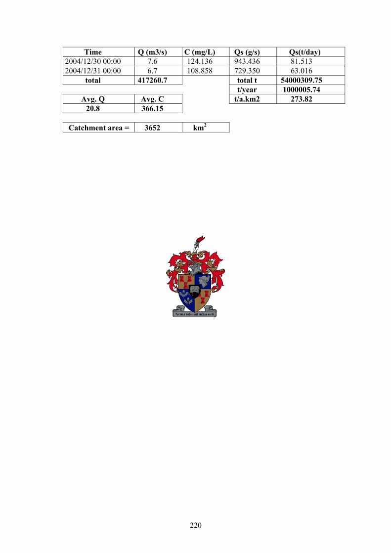
220

Time Q (m3/s) C (mg/L) Qs (g/s) Qs(t/day) 2004/12/30 00:00 7.6 124.136 943.436 81.513 2004/12/31 00:00 6.7 108.858 729.350 63.016

total 417260.7 total t 54000309.75 t/year 1000005.74

Avg. Q Avg. C t/a.km2 273.82 20.8 366.15

Catchment area = 3652 km2