IOP PUBLISHING and INTERNATIONAL ATOMIC ENERGY AGENCY NUCLEAR FUSION

Nucl. Fusion 49 (2009) 045011 (15pp) doi:10.1088/0029-5515/49/4/045011

2D characterization of core thermaltopology changes in controlledRFX-mod QSH statesFederica Bonomo, Alberto Alfier, Marco Gobbin, FulvioAuriemma, Paolo Franz, Lionello Marrelli, Roberto Pasqualotto,Gianluca Spizzo and David Terranova

Consorzio RFX, Euratom-ENEA Association, Corso Stati Uniti, 4 35127 Padova, Italy

E-mail: federica.bonomo@igi.cnr.it

Received 14 October 2008, accepted for publication 9 February 2009Published 20 March 2009Online at stacks.iop.org/NF/49/045011

AbstractIn the reversed field pinch RFX-mod device, the achievement of high plasma currents (Ip � 1.3 MA) has allowed theappearance of a new kind of large thermal structures emerging in the plasma core during the so-called quasi-singlehelicity (QSH) regimes. These structures correspond to a helical equilibrium established in the plasma, which hasbeen dubbed as the single helical axis (SHAx) state. The topological features of this new type of thermal structurescovering most of the plasma core have been experimentally investigated here. Analyses have been performed bymeans of three diagnostics, simultaneously and routinely running on RFX-mod: the soft x-ray (SXR) camera, theThomson scattering diagnostic for the electron temperature (Te) profile estimation and the SXR tomography. Inparticular, a 2D map reconstruction of Te has been performed: the core electron temperature asymmetries mostlyaccount for the ones in the reconstructed SXR emissivity. The magnetic topology of these QSH thermal structureshas also been analysed and numerically investigated by the Hamiltonian guiding centre code ORBIT: magnetic andthermal structures have been identified, in position and topological features. Also the Te profile temporal evolution,provided by the tomographic diagnostic and the SXR camera, has been investigated, showing that the transition toSHAx does not develop in a unique way.

PACS numbers: 52.25.Xz, 52.25.Tx, 52.30.Cv, 52.38.Ph, 52.55.Tn, 52.70.La

(Some figures in this article are in colour only in the electronic version)

1. Introduction

In the reversed field pinch (RFP), the presence of chaos inthe plasma core has long been considered to be intrinsic forsustaining the magnetic configuration. The broad spectrumof m = 1 MHD kink-tearing modes, with different n

(m and n being the poloidal and the toroidal mode numbers,respectively) and the Chirikov overlap of the associatedmagnetic islands, lead to a regime characterized by chaos,the so-called multiple helicity (MH) state. This view wassupported by the idea that the RFP dynamo, required tosustain the toroidal field in the core, implied as a necessitythe presence of a broad spectrum of m = 1 modes, witha turbulent cascade from low to high |n| numbers [1] (n isnegative for internal resonant modes). The theoretical effortshowing that the dynamo, in principle, can be sustained byonly one m = 1 mode (single helicity (SH)) [2, 3], togetherwith experimental observations of helical structures appearing

inside the plasma [4], has led to the confidence that the RFPcan exist in an ordered state which has been called quasi-singlehelicity (QSH).

In QSH, an m = 1, n0 mode dominates the magneticspectrum (|n0| ≈ R0/a, with R0 and a the major and minorradii of the torus), while a residual level of secondary modes(|n| > |n0|) is still present: this fact distinguishes the QSHwith respect to the pure, theoretical SH state, where nosecondary modes are present. The QSH regime has beenobserved to appear spontaneously in the RFX-mod experiment.The frequency of appearance of helical states-QSH, theirpersistence, their purity (i.e. the residual level of secondarymodes), the volume occupied by the island, and its temperatureare all aspects that have been improved by using a systemof feedback-controlled active coils, installed on RFX-mod in2005 [5]. This system consists of 192 saddle coils, uniformlycovering the external surface of the toroidal vessel, withindependent power supplies and real time controlled. This

0029-5515/09/045011+15$30.00 1 © 2009 IAEA, Vienna Printed in the UK

Nucl. Fusion 49 (2009) 045011 F. Bonomo et al

-0.4 -0.2 0.0 0.2 0.4r (m)

0.0

0.2

0.4

0.6

0.8

1.0

1.2

Te

(keV

)

#22090 (a)

-0.4 -0.2 0.0 0.2 0.4r (m)

#24932 (b)

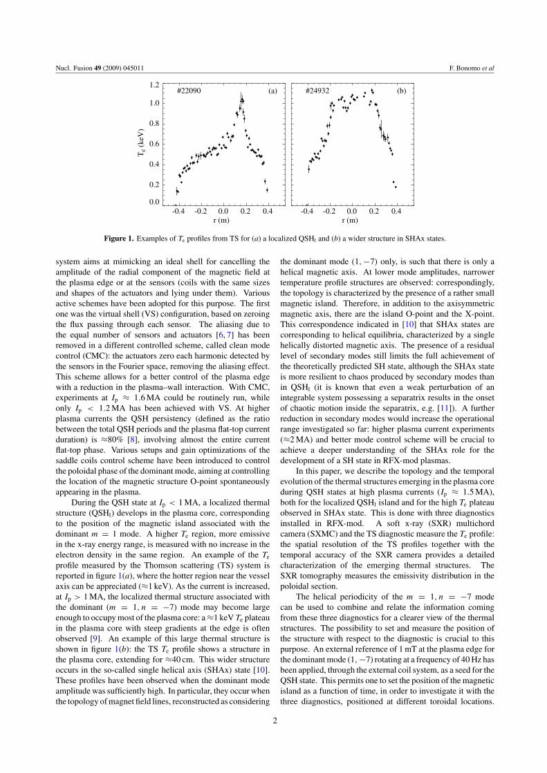
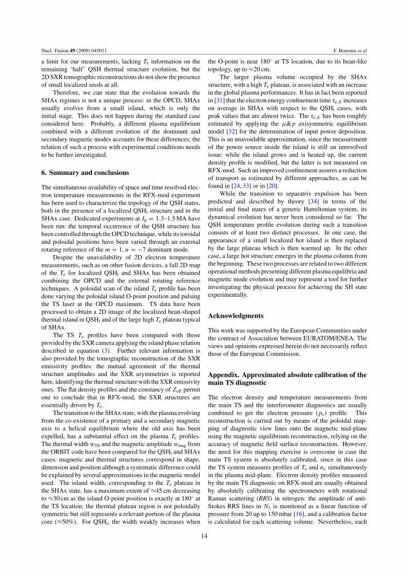
Figure 1. Examples of Te profiles from TS for (a) a localized QSHl and (b) a wider structure in SHAx states.

system aims at mimicking an ideal shell for cancelling theamplitude of the radial component of the magnetic field atthe plasma edge or at the sensors (coils with the same sizesand shapes of the actuators and lying under them). Variousactive schemes have been adopted for this purpose. The firstone was the virtual shell (VS) configuration, based on zeroingthe flux passing through each sensor. The aliasing due tothe equal number of sensors and actuators [6, 7] has beenremoved in a different controlled scheme, called clean modecontrol (CMC): the actuators zero each harmonic detected bythe sensors in the Fourier space, removing the aliasing effect.This scheme allows for a better control of the plasma edgewith a reduction in the plasma–wall interaction. With CMC,experiments at Ip ≈ 1.6 MA could be routinely run, whileonly Ip < 1.2 MA has been achieved with VS. At higherplasma currents the QSH persistency (defined as the ratiobetween the total QSH periods and the plasma flat-top currentduration) is ≈80% [8], involving almost the entire currentflat-top phase. Various setups and gain optimizations of thesaddle coils control scheme have been introduced to controlthe poloidal phase of the dominant mode, aiming at controllingthe location of the magnetic structure O-point spontaneouslyappearing in the plasma.

During the QSH state at Ip < 1 MA, a localized thermalstructure (QSHl) develops in the plasma core, correspondingto the position of the magnetic island associated with thedominant m = 1 mode. A higher Te region, more emissivein the x-ray energy range, is measured with no increase in theelectron density in the same region. An example of the Te

profile measured by the Thomson scattering (TS) system isreported in figure 1(a), where the hotter region near the vesselaxis can be appreciated (≈1 keV). As the current is increased,at Ip > 1 MA, the localized thermal structure associated withthe dominant (m = 1, n = −7) mode may become largeenough to occupy most of the plasma core: a ≈1 keV Te plateauin the plasma core with steep gradients at the edge is oftenobserved [9]. An example of this large thermal structure isshown in figure 1(b): the TS Te profile shows a structure inthe plasma core, extending for ≈40 cm. This wider structureoccurs in the so-called single helical axis (SHAx) state [10].These profiles have been observed when the dominant modeamplitude was sufficiently high. In particular, they occur whenthe topology of magnet field lines, reconstructed as considering

the dominant mode (1, −7) only, is such that there is only ahelical magnetic axis. At lower mode amplitudes, narrowertemperature profile structures are observed: correspondingly,the topology is characterized by the presence of a rather smallmagnetic island. Therefore, in addition to the axisymmetricmagnetic axis, there are the island O-point and the X-point.This correspondence indicated in [10] that SHAx states arecorresponding to helical equilibria, characterized by a singlehelically distorted magnetic axis. The presence of a residuallevel of secondary modes still limits the full achievement ofthe theoretically predicted SH state, although the SHAx stateis more resilient to chaos produced by secondary modes thanin QSHl (it is known that even a weak perturbation of anintegrable system possessing a separatrix results in the onsetof chaotic motion inside the separatrix, e.g. [11]). A furtherreduction in secondary modes would increase the operationalrange investigated so far: higher plasma current experiments(≈2 MA) and better mode control scheme will be crucial toachieve a deeper understanding of the SHAx role for thedevelopment of a SH state in RFX-mod plasmas.

In this paper, we describe the topology and the temporalevolution of the thermal structures emerging in the plasma coreduring QSH states at high plasma currents (Ip ≈ 1.5 MA),both for the localized QSHl island and for the high Te plateauobserved in SHAx state. This is done with three diagnosticsinstalled in RFX-mod. A soft x-ray (SXR) multichordcamera (SXMC) and the TS diagnostic measure the Te profile:the spatial resolution of the TS profiles together with thetemporal accuracy of the SXR camera provides a detailedcharacterization of the emerging thermal structures. TheSXR tomography measures the emissivity distribution in thepoloidal section.

The helical periodicity of the m = 1, n = −7 modecan be used to combine and relate the information comingfrom these three diagnostics for a clearer view of the thermalstructures. The possibility to set and measure the position ofthe structure with respect to the diagnostic is crucial to thispurpose. An external reference of 1 mT at the plasma edge forthe dominant mode (1,−7) rotating at a frequency of 40 Hz hasbeen applied, through the external coil system, as a seed for theQSH state. This permits one to set the position of the magneticisland as a function of time, in order to investigate it with thethree diagnostics, positioned at different toroidal locations.

2

Nucl. Fusion 49 (2009) 045011 F. Bonomo et al

For a typical 1.5 MA plasma discharge, lasting about 0.4 s,the structure crosses the region observed by each diagnostic6–7 times.

In addition, the need to investigate the QSH structures insimilar conditions (i.e. at the same instant in the QSH cycle)has led to the use of the oscillating poloidal current drive(OPCD) [12]. During OPCD operation, the toroidal field atthe edge is modulated with a given frequency and amplitude:this pinches the toroidal flux in the core and reduces the needfor the natural dynamo, allowing for a reduction in magneticfluctuations. In this work, the OPCD has been adopted becauseof the high QSH reproducibility.

The paper is organized as follows. In the next section, ashort description of the method used for the analyses presentedhere is provided. In section 2, the diagnostics used for thiswork are described. How the experimental measurementsfrom different diagnostics can be linked and compared isreported in section 3, followed by a detailed description of theexperimental operations in section 4. The more relevant resultsare described in section 5, where the 2D map of the thermalstructures and their temporal evolution are presented anddiscussed, for the QSHl states and the SHAx states. Finally,the main features of the thermal structures are summarized insection 6.

1.1. Method

We aim at characterizing the topological and temporalevolution of the thermal structure both in the QSH and inthe SHAx regimes. Measurements are taken from variousdiagnostics (see the next section for details): a SXMC anda TS diagnostic for Te estimation and the SXR tomographicsystem for SXR measurements. Their different toroidallocation requires inducing QSH states and forcing the structureinto a pre-defined poloidal position for being detectedsimultaneously by all the diagnostics. QSH states can beinduced by means of OPCD, while the structure positionis determined by adding an external reference magneticperturbation as seed to the magnetic boundary control system,making the seed rotate with an appropriate frequency. Moredetails on the method to induce QSH states and on controllingthe structure position can be found in section 4.

Measurements for the three diagnostics are then gatheredand correlated. Thanks to the reproducibility of the OPCDoscillation and of the externally introduced rotation, a largenumber of shots were performed, allowing one to gather TSTe profiles for a sufficient number of QSH and SHAx stateensembles. By modifying the external perturbation phase, wemanaged to measure theTe profiles along the plane diameters ofdifferent angles with respect to the O-point, thereby obtaininga 2D electron temperature map of the plasma core. Differentprocesses for achieving the SHAx state have been observedand investigated, thanks to the temporal resolution of the SXRdiagnostics.

2. Diagnostics

The thermal characterization of the QSH states in RFX-modtakes advantage of the availability of using diagnosticswith either high spatial or accurate temporal resolution,

simultaneously and routinely operating in RFX-mod: theSXMC and the TS for Te profile determination and the SXRtomography for plasma emissivity distribution reconstruction.Their different characteristics have allowed one to investigateand characterize the thermal content of the plasma column,identifying thermal structures and their evolution during QSHperiods.

The SXMC for Te determination [13] consists of fourgroups of five photodiodes each, measuring the SXR plasmaemissivity through four pinholes, and it is installed at 262.5toroidal degrees in a vacuum vessel upper port. Each pinholehouses a beryllium filter with different thicknesses (36, 47, 72and 96 µm), acting as the energy selector. The 20 lines of sightdefined by the diodes and the pinholes look at the same poloidalsection, being coupled two by two. This results in a fan of tenpairs of chords covering the outboard section of the RFX-modplasma. The current generated in the detectors is of the order ofnanoamperes, and it is proportional to the absorbed SXR powerimpinging on it. The two-foil technique [14, 15] is appliedto the brightness of each pair of chords to estimate Te. It isderived from the ratio between the SXR brightnesses measuredthrough different beryllium foils but facing the same plasmaregion: the ratio depends mainly on the peak temperature alongthe considered lines of sight [14]. Considering the 10 pairsof chords, a 10 points Te profile is obtained. The diagnosticdetects detailed features of the Te profiles (up to 4.5 cm) with atime accuracy of a few kilohertz. There are several sources oferrors that affect these measurements: the intrinsic noise of thediodes, the global noise caused by the electronic components,the uncertainties of the silicon detector effective areas and ofthe beryllium foil thickness. Considering all these sources, theconsequent error in the temperature estimation is of the orderof 8% at a temperature of about 500 eV [13].

The TS system [16], installed at 82.5 toroidal degrees ofthe RFX-mod vessel, provides Te profiles with 84 points and0.7 cm resolution along almost an entire equatorial diameter(−0.96 to 0.84 r/a). The custom built Nd : YLF laser(1053 nm) produces a fast (�50 Hz) burst of 10 high energypulses suitable for measuring the profile evolution in theplasma discharge of RFX-mod. The TS signal is collectedat ≈90◦ scattering angle from the incident beam throughthree objective lenses which image the laser beam onto a rowof 84 pairs of optical fibres. Fibres are then arranged intobundles, fed to 28 spectrometers. Each bundle is made ofthree different length pairs of fibres. Such a bundle serves as amultiplexing system which allocates 3 scattering volumes perpolychromator by means of optical delay lines: the differentlengths of the fibres (14 m difference) produce three pulsesseparated by the time required to run the extra length (70 ns).In each spectrometer, the TS signal is cascaded through fourspectral channels in a zigzag path, using a series of relaylenses, with four APD detectors optimized for the IR (3 mmdiameter active area). The collection efficiency of the systemallows measuring Te profiles at an electron density as lowas 1 × 1019 m−3. Signal waveforms are finally recorded bywaveform digitizers, so that the three time separated TS pulsesare distinguished. As a further advantage, the known pulseshape can be fitted to the measured waveform at a fixed time,recovering well even the weak signals from high noise.

The SXR tomographic diagnostic (SXT) measures thex-ray radiation emitted from the plasma poloidal cross-section

3

Nucl. Fusion 49 (2009) 045011 F. Bonomo et al

Top view of RFX-mod vessel

-3 -2 -1 0 1 2 3R (m)

-3

-2

-1

0

1

2

3

R (

m)

SXT

TS

SXMC

(a)

82.5 º

-0.6 -0.4 -0.2 0.0 0.2 0.4 0.6R (m)

-0.6

-0.4

-0.2

0.0

0.2

0.4

0.6

R (

m)

(b)TS

262.5 º

-0.6 -0.4 -0.2 0.0 0.2 0.4 0.6R (m)

-0.6

-0.4

-0.2

0.0

0.2

0.4

0.6

R (

m)

(d)SXMC

202.5 º

-0.6 -0.4 -0.2 0.0 0.2 0.4 0.6R (m)

-0.6

-0.4

-0.2

0.0

0.2

0.4

0.6

R (

m)

(c)SXT

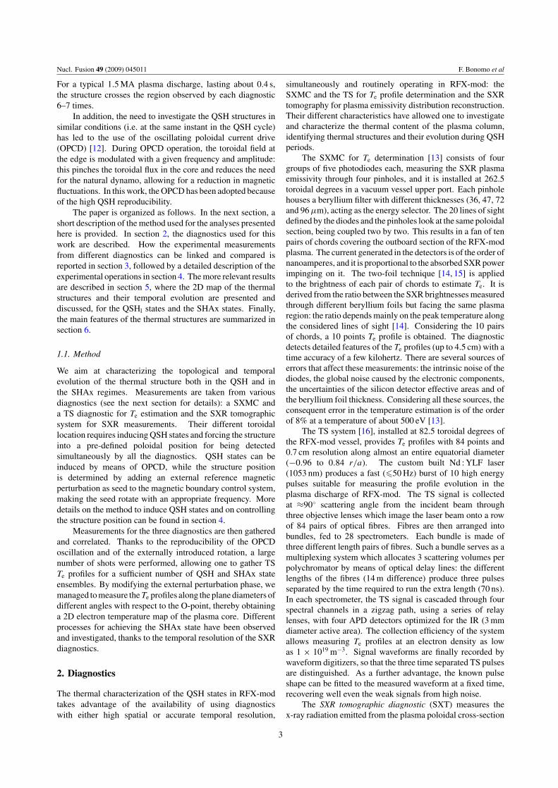
Figure 2. (a) Top view of the RFX-mod toroidal vessel, with the three diagnostic locations highlighted: TS, SXT and SXMC. Lines of sightof (b) TS, (c) SXT and (d) SXMC.

at 202.5 toroidal degrees along 78 collimated lines of sight,permitting reconstruction of the plasma emissivity by meansof tomographic algorithms [17]. The lines of sight, emanatedby four cameras set in different portholes, uniformly coverthe RFX-mod cross-section. Beryllium filters of 31 µm areused to select only the bremsstrahlung component of the SXRemissivity spectrum. All the Be foils are mounted on curvedsupports, installed in 2007 in order to avoid the systematic errorreported in [17]: in this way, all the lines of sight look at theplasma through Be filters with exactly the same thickness, andno corrections are needed to render all the experimental datauniform. The algorithms used for tomographic reconstructionsare those based on Fourier–Bessels series expansions [17]: thebrightness and the emissivity are expanded in a truncated (dueto the finite number of measurements) Fourier series; then theFourier components are radially expanded over a truncated setof Bessel polynomials. The reconstructions are traced back toa matrix inversion, and a map of the SXR plasma emissivitydistribution is obtained. The spatial resolution is limited by thenumber of lines of sight and their distribution in the RFX-modvessel: localized structures larger than the distance betweentwo adjacent chords, and with poloidal mode number up tom = 2, can be identified. The temporal resolution is insteaddictated by the electronic chain of the signal processing andcan be up to hundreds of kilohertz at medium amplifying gainsettings.

The different toroidal locations of the three diagnosticsin the RFX-mod vessel are reported in the top view of theRFX-mod vessel in figure 2(a). The scattering volume of the

TS diagnostic in the mid-plane is shown in frame (b); thelines of sight of the SXR tomography (SXT) are illustratedin (c) and the 10 pairs of chords of the SXR camera (SXMC)are displayed in (d). The diagnostics measure differentplasma regions but combining together their results, the mainthermal features of RFX-mod plasmas can be identified.Asymmetric structures such as those emerging during QSHcan be investigated: as an example, in correspondence tothe magnetic island, at the toroidal location of SXT a bean-shaped more emissive localized region is observed (centralred region in the contour plot of figure 3(a)) and a hotterlocalized region emerges in the core of the Te profile measuredby TS (figure 3(b)) and SXMC (figure 3(c)). The way allthese measurements are gathered and analysed together as ifcollected at the same toroidal position is described in section 3.

3. Comparison of thermal profiles in helicalcoordinates

The interpretation of the measurements provided by thethree systems is not fully straightforward during QSH statebecause of several factors: (1) different toroidal locations ofdiagnostics, (2) intrinsic limit of integrated measurementsand (3) dependence of measurements on different plasmaparameters (e.g. density or impurities content). The firsttwo aspects are mainly related to the helical feature of theQSH state. The nth helicity of the dominant m = 1 modedetermines the poloidal positions of the O-point of the QSH

4

Nucl. Fusion 49 (2009) 045011 F. Bonomo et al

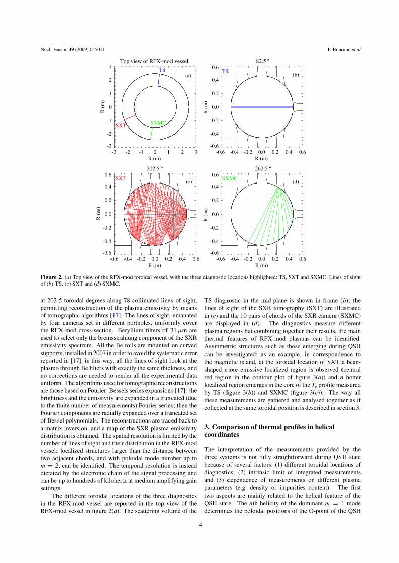
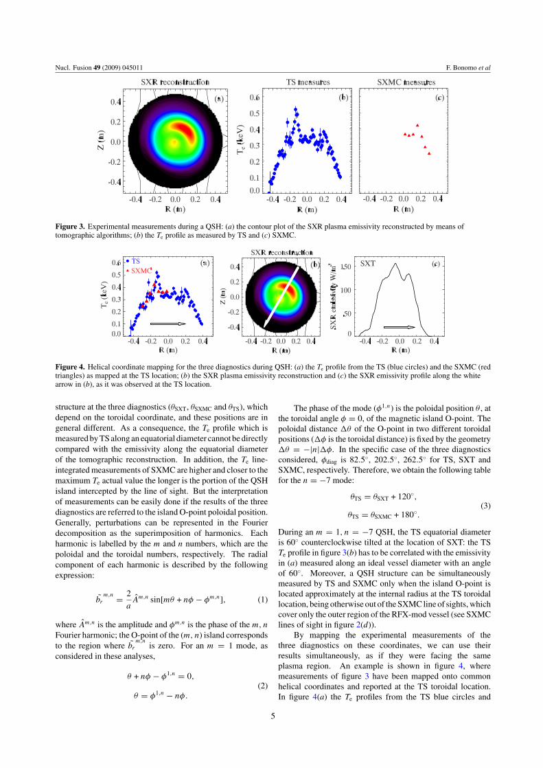
Figure 3. Experimental measurements during a QSH: (a) the contour plot of the SXR plasma emissivity reconstructed by means oftomographic algorithms; (b) the Te profile as measured by TS and (c) SXMC.

Figure 4. Helical coordinate mapping for the three diagnostics during QSH: (a) the Te profile from the TS (blue circles) and the SXMC (redtriangles) as mapped at the TS location; (b) the SXR plasma emissivity reconstruction and (c) the SXR emissivity profile along the whitearrow in (b), as it was observed at the TS location.

structure at the three diagnostics (θSXT, θSXMC and θTS), whichdepend on the toroidal coordinate, and these positions are ingeneral different. As a consequence, the Te profile which ismeasured by TS along an equatorial diameter cannot be directlycompared with the emissivity along the equatorial diameterof the tomographic reconstruction. In addition, the Te line-integrated measurements of SXMC are higher and closer to themaximum Te actual value the longer is the portion of the QSHisland intercepted by the line of sight. But the interpretationof measurements can be easily done if the results of the threediagnostics are referred to the island O-point poloidal position.Generally, perturbations can be represented in the Fourierdecomposition as the superimposition of harmonics. Eachharmonic is labelled by the m and n numbers, which are thepoloidal and the toroidal numbers, respectively. The radialcomponent of each harmonic is described by the followingexpression:

br

m,n = 2

aAm,n sin[mθ + nφ − φm,n], (1)

where Am,n is the amplitude and φm,n is the phase of the m, n

Fourier harmonic; the O-point of the (m, n) island correspondsto the region where br

m,nis zero. For an m = 1 mode, as

considered in these analyses,

θ + nφ − φ1,n = 0,

θ = φ1,n − nφ.

(2)

The phase of the mode (φ1,n) is the poloidal position θ , atthe toroidal angle φ = 0, of the magnetic island O-point. Thepoloidal distance �θ of the O-point in two different toroidalpositions (�φ is the toroidal distance) is fixed by the geometry�θ = −|n|�φ. In the specific case of the three diagnosticsconsidered, φdiag is 82.5◦, 202.5◦, 262.5◦ for TS, SXT andSXMC, respectively. Therefore, we obtain the following tablefor the n = −7 mode:

θTS = θSXT + 120◦,

θTS = θSXMC + 180◦.(3)

During an m = 1, n = −7 QSH, the TS equatorial diameteris 60◦ counterclockwise tilted at the location of SXT: the TSTe profile in figure 3(b) has to be correlated with the emissivityin (a) measured along an ideal vessel diameter with an angleof 60◦. Moreover, a QSH structure can be simultaneouslymeasured by TS and SXMC only when the island O-point islocated approximately at the internal radius at the TS toroidallocation, being otherwise out of the SXMC line of sights, whichcover only the outer region of the RFX-mod vessel (see SXMClines of sight in figure 2(d)).

By mapping the experimental measurements of thethree diagnostics on these coordinates, we can use theirresults simultaneously, as if they were facing the sameplasma region. An example is shown in figure 4, wheremeasurements of figure 3 have been mapped onto commonhelical coordinates and reported at the TS toroidal location.In figure 4(a) the Te profiles from the TS blue circles and

5

Nucl. Fusion 49 (2009) 045011 F. Bonomo et al

from the SXMC red triangles are illustrated: the SXMCTe estimates correspond to measurements in the internalregion of the RFX-mod vessel and are well superimposedto TS measurements. The localized hotter region, whichcorresponds to the island O-point of the m = 1, n = −7dominant mode, observed by both systems, is detected indetail. The SXR emissivity reconstruction (b) shows amore emissive bean-shaped structure in correspondence to themagnetic island. The superimposed white arrow is obtainedfrom equation (3) and corresponds to the radial coordinate ofthe TS profile (e.g. the laser path) with respect to the n = −7mode at the SXT location. The SXR reconstructed emissivityalong this arrow is shown in figure 4(c). As a result, a detailedspatial and topological characterization of the QSH thermalstructure can be done.

To summarize, the TS system gives information on Te

in the magnetic island, its maximum value and the thermalisland shape, which are supported and confirmed by SXMCmeasurements. The latter measures the temporal evolutionof the structure: the way the island heats up and the way itevolves during QSH. The SXR structure associated with themagnetic island gives information on the plasma topology,such as its radial and poloidal extension (as in figure 4(b))and its evolution.

Additional issues in measurement comparison have to beconsidered, mostly based on the different plasma parameters onwhich these experimental measurements depend. Their signal-to-noise level may be reduced or even corrupted, e.g. [16]by an intense plasma light level, which is typically higherthan usual in case of strong localized plasma–wall interaction(e.g. at the locked mode location, that is when the magneticmodes are phase-locked and locked to the wall, resulting in aplasma column deformation which intercepts the first wall): theconsequent limitation is that all three measurements could notbe simultaneously available. Moreover, SXR measurementsalso depend on the electron density (ne) and the plasmaimpurity content (the effective charge, Zeff ): for RFX-mod itis reasonable to assume a constant Zeff in the plasma coreas in [18], while no evidence of impurity entrapment has yetbeen found in the QSH structures [19]. Considerations on theelectron density and its profiles are reported in section 5.3.

4. QSH control for diagnostic purpose

Due to the different locations of the diagnostics, the laserrepetition rate of TS and the fact that QSH is unpredictable ina standard plasma discharge, the thermal QSH investigationwould require a large number of discharges. A relevantimprovement has been added by combining OPCD with anexternal rotating reference for the dominant mode, in order totrigger the QSH onset at the right time with the right O-pointposition.

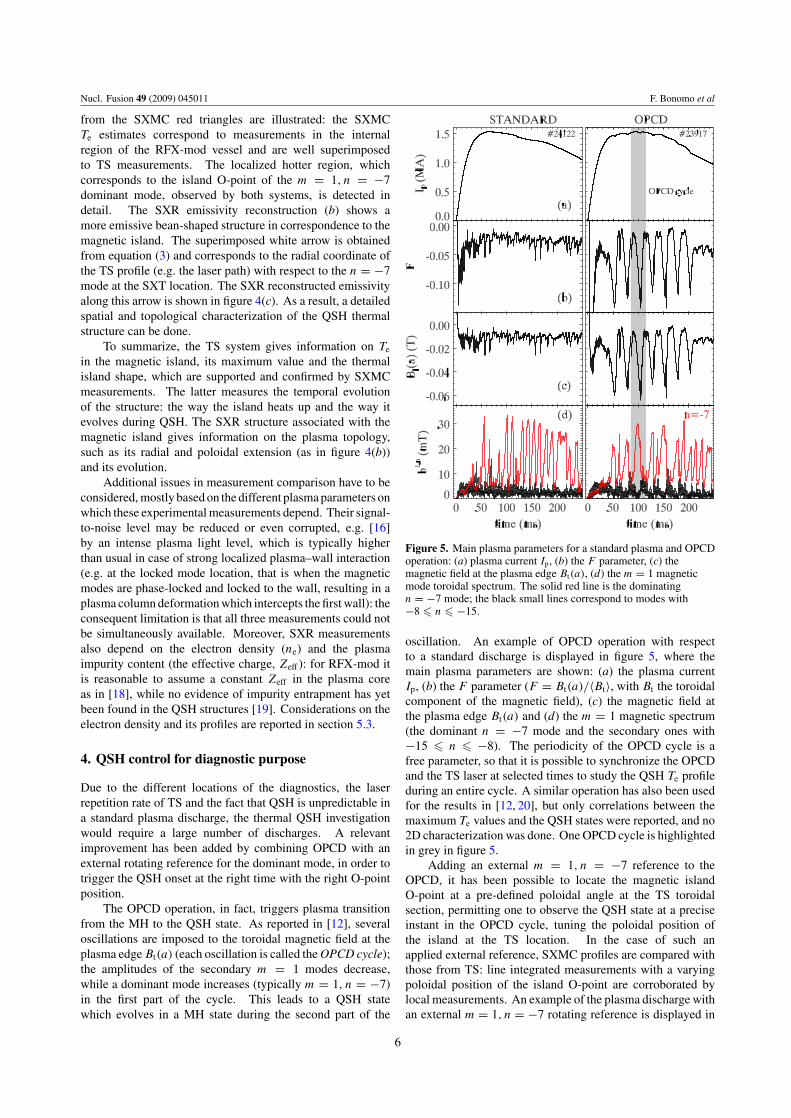
The OPCD operation, in fact, triggers plasma transitionfrom the MH to the QSH state. As reported in [12], severaloscillations are imposed to the toroidal magnetic field at theplasma edge Bt(a) (each oscillation is called the OPCD cycle);the amplitudes of the secondary m = 1 modes decrease,while a dominant mode increases (typically m = 1, n = −7)in the first part of the cycle. This leads to a QSH statewhich evolves in a MH state during the second part of the

Figure 5. Main plasma parameters for a standard plasma and OPCDoperation: (a) plasma current Ip, (b) the F parameter, (c) themagnetic field at the plasma edge Bt(a), (d) the m = 1 magneticmode toroidal spectrum. The solid red line is the dominatingn = −7 mode; the black small lines correspond to modes with−8 � n � −15.

oscillation. An example of OPCD operation with respectto a standard discharge is displayed in figure 5, where themain plasma parameters are shown: (a) the plasma currentIp, (b) the F parameter (F = Bt(a)/〈Bt〉, with Bt the toroidalcomponent of the magnetic field), (c) the magnetic field atthe plasma edge Bt(a) and (d) the m = 1 magnetic spectrum(the dominant n = −7 mode and the secondary ones with−15 � n � −8). The periodicity of the OPCD cycle is afree parameter, so that it is possible to synchronize the OPCDand the TS laser at selected times to study the QSH Te profileduring an entire cycle. A similar operation has also been usedfor the results in [12, 20], but only correlations between themaximum Te values and the QSH states were reported, and no2D characterization was done. One OPCD cycle is highlightedin grey in figure 5.

Adding an external m = 1, n = −7 reference to theOPCD, it has been possible to locate the magnetic islandO-point at a pre-defined poloidal angle at the TS toroidalsection, permitting one to observe the QSH state at a preciseinstant in the OPCD cycle, tuning the poloidal position ofthe island at the TS location. In the case of such anapplied external reference, SXMC profiles are compared withthose from TS: line integrated measurements with a varyingpoloidal position of the island O-point are corroborated bylocal measurements. An example of the plasma discharge withan external m = 1, n = −7 rotating reference is displayed in

6

Nucl. Fusion 49 (2009) 045011 F. Bonomo et al

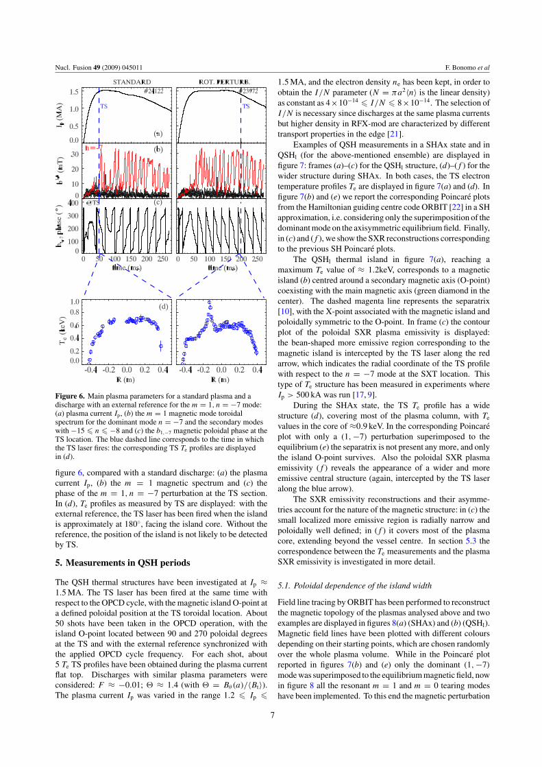
Figure 6. Main plasma parameters for a standard plasma and adischarge with an external reference for the m = 1, n = −7 mode:(a) plasma current Ip, (b) the m = 1 magnetic mode toroidalspectrum for the dominant mode n = −7 and the secondary modeswith −15 � n � −8 and (c) the b1,−7 magnetic poloidal phase at theTS location. The blue dashed line corresponds to the time in whichthe TS laser fires: the corresponding TS Te profiles are displayedin (d).

figure 6, compared with a standard discharge: (a) the plasmacurrent Ip, (b) the m = 1 magnetic spectrum and (c) thephase of the m = 1, n = −7 perturbation at the TS section.In (d), Te profiles as measured by TS are displayed: with theexternal reference, the TS laser has been fired when the islandis approximately at 180◦, facing the island core. Without thereference, the position of the island is not likely to be detectedby TS.

5. Measurements in QSH periods

The QSH thermal structures have been investigated at Ip ≈1.5 MA. The TS laser has been fired at the same time withrespect to the OPCD cycle, with the magnetic island O-point ata defined poloidal position at the TS toroidal location. About50 shots have been taken in the OPCD operation, with theisland O-point located between 90 and 270 poloidal degreesat the TS and with the external reference synchronized withthe applied OPCD cycle frequency. For each shot, about5 Te TS profiles have been obtained during the plasma currentflat top. Discharges with similar plasma parameters wereconsidered: F ≈ −0.01; � ≈ 1.4 (with � = Bθ(a)/〈Bt〉).The plasma current Ip was varied in the range 1.2 � Ip �

1.5 MA, and the electron density ne has been kept, in order toobtain the I/N parameter (N = πa2〈n〉 is the linear density)as constant as 4×10−14 � I/N � 8×10−14. The selection ofI/N is necessary since discharges at the same plasma currentsbut higher density in RFX-mod are characterized by differenttransport properties in the edge [21].

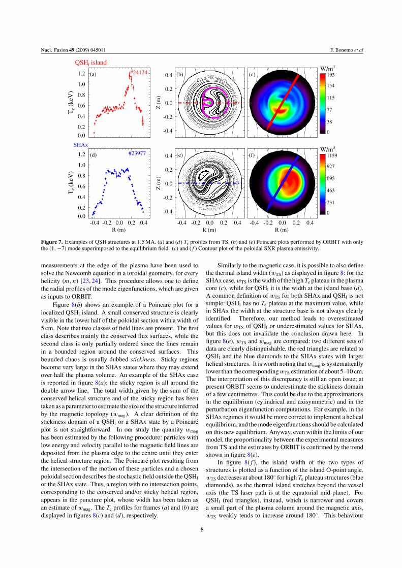
Examples of QSH measurements in a SHAx state and inQSHl (for the above-mentioned ensemble) are displayed infigure 7: frames (a)–(c) for the QSHl structure, (d)–( f ) for thewider structure during SHAx. In both cases, the TS electrontemperature profiles Te are displayed in figure 7(a) and (d). Infigure 7(b) and (e) we report the corresponding Poincare plotsfrom the Hamiltonian guiding centre code ORBIT [22] in a SHapproximation, i.e. considering only the superimposition of thedominant mode on the axisymmetric equilibrium field. Finally,in (c) and ( f ), we show the SXR reconstructions correspondingto the previous SH Poincare plots.

The QSHl thermal island in figure 7(a), reaching amaximum Te value of ≈ 1.2keV, corresponds to a magneticisland (b) centred around a secondary magnetic axis (O-point)coexisting with the main magnetic axis (green diamond in thecenter). The dashed magenta line represents the separatrix[10], with the X-point associated with the magnetic island andpoloidally symmetric to the O-point. In frame (c) the contourplot of the poloidal SXR plasma emissivity is displayed:the bean-shaped more emissive region corresponding to themagnetic island is intercepted by the TS laser along the redarrow, which indicates the radial coordinate of the TS profilewith respect to the n = −7 mode at the SXT location. Thistype of Te structure has been measured in experiments whereIp > 500 kA was run [17, 9].

During the SHAx state, the TS Te profile has a widestructure (d), covering most of the plasma column, with Te

values in the core of ≈0.9 keV. In the corresponding Poincareplot with only a (1, −7) perturbation superimposed to theequilibrium (e) the separatrix is not present any more, and onlythe island O-point survives. Also the poloidal SXR plasmaemissivity ( f ) reveals the appearance of a wider and moreemissive central structure (again, intercepted by the TS laseralong the blue arrow).

The SXR emissivity reconstructions and their asymme-tries account for the nature of the magnetic structure: in (c) thesmall localized more emissive region is radially narrow andpoloidally well defined; in ( f ) it covers most of the plasmacore, extending beyond the vessel centre. In section 5.3 thecorrespondence between the Te measurements and the plasmaSXR emissivity is investigated in more detail.

5.1. Poloidal dependence of the island width

Field line tracing by ORBIT has been performed to reconstructthe magnetic topology of the plasmas analysed above and twoexamples are displayed in figures 8(a) (SHAx) and (b) (QSHl).Magnetic field lines have been plotted with different coloursdepending on their starting points, which are chosen randomlyover the whole plasma volume. While in the Poincare plotreported in figures 7(b) and (e) only the dominant (1, −7)

mode was superimposed to the equilibrium magnetic field, nowin figure 8 all the resonant m = 1 and m = 0 tearing modeshave been implemented. To this end the magnetic perturbation

7

Nucl. Fusion 49 (2009) 045011 F. Bonomo et al

-0.4 -0.2 0.0 0.2 0.4R (m)

0.0

0.2

0.4

0.6

0.8

1.0

1.2

Te (

keV

)

(d) #23977

SHAx

0.0

0.2

0.4

0.6

0.8

1.0

1.2T

e (ke

V)

(a) #24124

QSHl island

-0.4 -0.2 0.0 0.2 0.4R (m)

-0.4

-0.2

0.0

0.2

0.4Z

(m

)(e)

-0.4

-0.2

0.0

0.2

0.4

Z (

m)

(b)

(c) W/m3

0

38

77

115

154

193

-0.4 -0.2 0.0 0.2 0.4R (m)

(f) W/m3

0

231

463

695

927

1159

Figure 7. Examples of QSH structures at 1.5 MA. (a) and (d) Te profiles from TS. (b) and (e) Poincare plots performed by ORBIT with onlythe (1, −7) mode superimposed to the equilibrium field. (c) and ( f ) Contour plot of the poloidal SXR plasma emissivity.

measurements at the edge of the plasma have been used tosolve the Newcomb equation in a toroidal geometry, for everyhelicity (m, n) [23, 24]. This procedure allows one to definethe radial profiles of the mode eigenfunctions, which are givenas inputs to ORBIT.

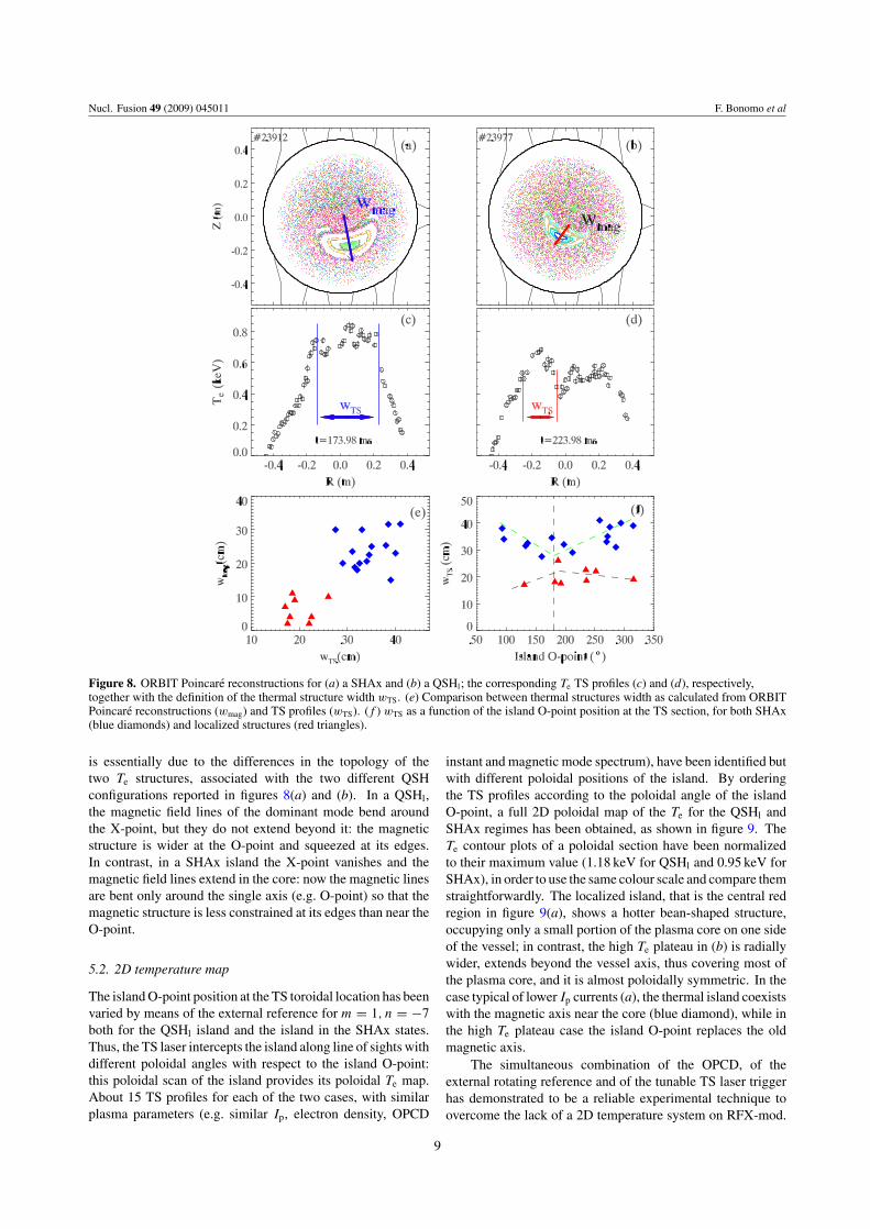
Figure 8(b) shows an example of a Poincare plot for alocalized QSHl island. A small conserved structure is clearlyvisible in the lower half of the poloidal section with a width of5 cm. Note that two classes of field lines are present. The firstclass describes mainly the conserved flux surfaces, while thesecond class is only partially ordered since the lines remainin a bounded region around the conserved surfaces. Thisbounded chaos is usually dubbed stickiness. Sticky regionsbecome very large in the SHAx states where they may extendover half the plasma volume. An example of the SHAx caseis reported in figure 8(a): the sticky region is all around thedouble arrow line. The total width given by the sum of theconserved helical structure and of the sticky region has beentaken as a parameter to estimate the size of the structure inferredby the magnetic topology (wmag). A clear definition of thestickiness domain of a QSHl or a SHAx state by a Poincareplot is not straightforward. In our study the quantity wmag

has been estimated by the following procedure: particles withlow energy and velocity parallel to the magnetic field lines aredeposited from the plasma edge to the centre until they enterthe helical structure region. The Poincare plot resulting fromthe intersection of the motion of these particles and a chosenpoloidal section describes the stochastic field outside the QSHl

or the SHAx state. Thus, a region with no intersection points,corresponding to the conserved and/or sticky helical region,appears in the puncture plot, whose width has been taken asan estimate of wmag. The Te profiles for frames (a) and (b) aredisplayed in figures 8(c) and (d), respectively.

Similarly to the magnetic case, it is possible to also definethe thermal island width (wTS) as displayed in figure 8: for theSHAx case, wTS is the width of the high Te plateau in the plasmacore (c), while for QSHl it is the width at the island base (d).A common definition of wTS for both SHAx and QSHl is notsimple: QSHl has no Te plateau at the maximum value, whilein SHAx the width at the structure base is not always clearlyidentified. Therefore, our method leads to overestimatedvalues for wTS of QSHl or underestimated values for SHAx,but this does not invalidate the conclusion drawn here. Infigure 8(e), wTS and wmag are compared: two different sets ofdata are clearly distinguishable, the red triangles are related toQSHl and the blue diamonds to the SHAx states with largerhelical structures. It is worth noting that wmag is systematicallylower than the corresponding wTS estimation of about 5–10 cm.The interpretation of this discrepancy is still an open issue; atpresent ORBIT seems to underestimate the stickiness domainof a few centimetres. This could be due to the approximationsin the equilibrium (cylindrical and axisymmetric) and in theperturbation eigenfunction computations. For example, in theSHAx regimes it would be more correct to implement a helicalequilibrium, and the mode eigenfunctions should be calculatedon this new equilibrium. Anyway, even within the limits of ourmodel, the proportionality between the experimental measuresfrom TS and the estimates by ORBIT is confirmed by the trendshown in figure 8(e).

In figure 8( f ), the island width of the two types ofstructures is plotted as a function of the island O-point angle.wTS decreases at about 180◦ for high Te plateau structures (bluediamonds), as the thermal island stretches beyond the vesselaxis (the TS laser path is at the equatorial mid-plane). ForQSHl (red triangles), instead, which is narrower and coversa small part of the plasma column around the magnetic axis,wTS weakly tends to increase around 180◦. This behaviour

8

Nucl. Fusion 49 (2009) 045011 F. Bonomo et al

º

Figure 8. ORBIT Poincare reconstructions for (a) a SHAx and (b) a QSHl; the corresponding Te TS profiles (c) and (d), respectively,together with the definition of the thermal structure width wTS. (e) Comparison between thermal structures width as calculated from ORBITPoincare reconstructions (wmag) and TS profiles (wTS). ( f ) wTS as a function of the island O-point position at the TS section, for both SHAx(blue diamonds) and localized structures (red triangles).

is essentially due to the differences in the topology of thetwo Te structures, associated with the two different QSHconfigurations reported in figures 8(a) and (b). In a QSHl,the magnetic field lines of the dominant mode bend aroundthe X-point, but they do not extend beyond it: the magneticstructure is wider at the O-point and squeezed at its edges.In contrast, in a SHAx island the X-point vanishes and themagnetic field lines extend in the core: now the magnetic linesare bent only around the single axis (e.g. O-point) so that themagnetic structure is less constrained at its edges than near theO-point.

5.2. 2D temperature map

The island O-point position at the TS toroidal location has beenvaried by means of the external reference for m = 1, n = −7both for the QSHl island and the island in the SHAx states.Thus, the TS laser intercepts the island along line of sights withdifferent poloidal angles with respect to the island O-point:this poloidal scan of the island provides its poloidal Te map.About 15 TS profiles for each of the two cases, with similarplasma parameters (e.g. similar Ip, electron density, OPCD

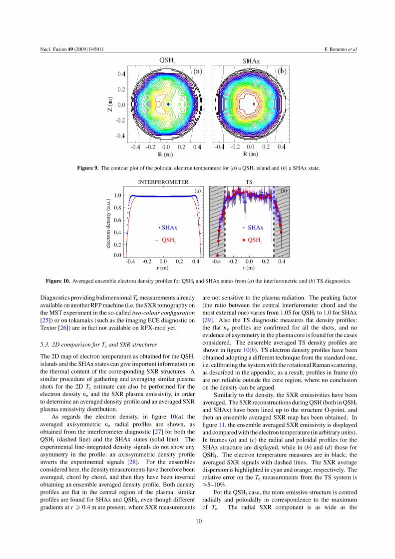
instant and magnetic mode spectrum), have been identified butwith different poloidal positions of the island. By orderingthe TS profiles according to the poloidal angle of the islandO-point, a full 2D poloidal map of the Te for the QSHl andSHAx regimes has been obtained, as shown in figure 9. TheTe contour plots of a poloidal section have been normalizedto their maximum value (1.18 keV for QSHl and 0.95 keV forSHAx), in order to use the same colour scale and compare themstraightforwardly. The localized island, that is the central redregion in figure 9(a), shows a hotter bean-shaped structure,occupying only a small portion of the plasma core on one sideof the vessel; in contrast, the high Te plateau in (b) is radiallywider, extends beyond the vessel axis, thus covering most ofthe plasma core, and it is almost poloidally symmetric. In thecase typical of lower Ip currents (a), the thermal island coexistswith the magnetic axis near the core (blue diamond), while inthe high Te plateau case the island O-point replaces the oldmagnetic axis.

The simultaneous combination of the OPCD, of theexternal rotating reference and of the tunable TS laser triggerhas demonstrated to be a reliable experimental technique toovercome the lack of a 2D temperature system on RFX-mod.

9

Nucl. Fusion 49 (2009) 045011 F. Bonomo et al

Figure 9. The contour plot of the poloidal electron temperature for (a) a QSHl island and (b) a SHAx state.

INTERFEROMETER

-0.4 -0.2 0.0 0.2 0.4r (m)

0.0

0.2

0.4

0.6

0.8

1.0

elec

tron

den

sity

(a.

u.)

SHAx

QSHl

(a)

TS

-0.4 -0.2 0.0 0.2 0.4r (m)

SHAx

QSHl

(b)

Figure 10. Averaged ensemble electron density profiles for QSHl and SHAx states from (a) the interferometric and (b) TS diagnostics.

Diagnostics providing bidimensional Te measurements alreadyavailable on another RFP machine (i.e. the SXR tomography onthe MST experiment in the so-called two-colour configuration[25]) or on tokamaks (such as the imaging ECE diagnostic onTextor [26]) are in fact not available on RFX-mod yet.

5.3. 2D comparison for Te and SXR structures

The 2D map of electron temperature as obtained for the QSHl

islands and the SHAx states can give important information onthe thermal content of the corresponding SXR structures. Asimilar procedure of gathering and averaging similar plasmashots for the 2D Te estimate can also be performed for theelectron density ne and the SXR plasma emissivity, in orderto determine an averaged density profile and an averaged SXRplasma emissivity distribution.

As regards the electron density, in figure 10(a) theaveraged axisymmetric ne radial profiles are shown, asobtained from the interferometer diagnostic [27] for both theQSHl (dashed line) and the SHAx states (solid line). Theexperimental line-integrated density signals do not show anyasymmetry in the profile: an axissymmetric density profileinverts the experimental signals [28]. For the ensemblesconsidered here, the density measurements have therefore beenaveraged, chord by chord, and then they have been invertedobtaining an ensemble averaged density profile. Both densityprofiles are flat in the central region of the plasma: similarprofiles are found for SHAx and QSHl, even though differentgradients at r � 0.4 m are present, where SXR measurements

are not sensitive to the plasma radiation. The peaking factor(the ratio between the central interferometer chord and themost external one) varies from 1.05 for QSHl to 1.0 for SHAx[29]. Also the TS diagnostic measures flat density profiles:the flat ne profiles are confirmed for all the shots, and noevidence of asymmetry in the plasma core is found for the casesconsidered. The ensemble averaged TS density profiles areshown in figure 10(b). TS electron density profiles have beenobtained adopting a different technique from the standard one,i.e. calibrating the system with the rotational Raman scattering,as described in the appendix; as a result, profiles in frame (b)are not reliable outside the core region, where no conclusionon the density can be argued.

Similarly to the density, the SXR emissivities have beenaveraged. The SXR reconstructions during QSH (both in QSHl

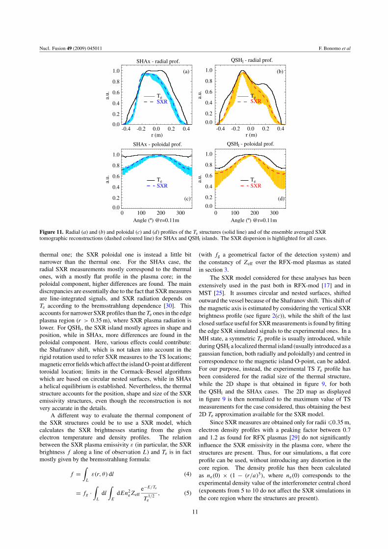
and SHAx) have been lined up to the structure O-point, andthen an ensemble averaged SXR map has been obtained. Infigure 11, the ensemble averaged SXR emissivity is displayedand compared with the electron temperature (in arbitrary units).In frames (a) and (c) the radial and poloidal profiles for theSHAx structure are displayed, while in (b) and (d) those forQSHl. The electron temperature measures are in black; theaveraged SXR signals with dashed lines. The SXR averagedispersion is highlighted in cyan and orange, respectively. Therelative error on the Te measurements from the TS system is≈5–10%.

For the QSHl case, the more emissive structure is centredradially and poloidally in correspondence to the maximumof Te. The radial SXR component is as wide as the

10

Nucl. Fusion 49 (2009) 045011 F. Bonomo et al

SHAx - radial prof.

-0.4 -0.2 0.0 0.2 0.4r (m)

0.0

0.2

0.4

0.6

0.8

1.0

a.u. Te

SXR

(a)

QSHl - radial prof.

-0.4 -0.2 0.0 0.2 0.4r (m)

0.0

0.2

0.4

0.6

0.8

1.0

a.u. Te

SXR

(b)

SHAx - poloidal prof.

0 100 200 300Angle (º) @r=0.11m

0.0

0.2

0.4

0.6

0.8

1.0

a.u. Te

SXR

(c)

QSHl - poloidal prof.

0 100 200 300Angle (º) @r=0.11m

0.0

0.2

0.4

0.6

0.8

1.0

a.u. Te

SXR

(d)

Figure 11. Radial (a) and (b) and poloidal (c) and (d) profiles of the Te structures (solid line) and of the ensemble averaged SXRtomographic reconstructions (dashed coloured line) for SHAx and QSHl islands. The SXR dispersion is highlighted for all cases.

thermal one; the SXR poloidal one is instead a little bitnarrower than the thermal one. For the SHAx case, theradial SXR measurements mostly correspond to the thermalones, with a mostly flat profile in the plasma core; in thepoloidal component, higher differences are found. The maindiscrepancies are essentially due to the fact that SXR measuresare line-integrated signals, and SXR radiation depends onTe according to the bremsstrahlung dependence [30]. Thisaccounts for narrower SXR profiles than the Te ones in the edgeplasma region (r > 0.35 m), where SXR plasma radiation islower. For QSHl, the SXR island mostly agrees in shape andposition, while in SHAx, more differences are found in thepoloidal component. Here, various effects could contribute:the Shafranov shift, which is not taken into account in therigid rotation used to refer SXR measures to the TS locations;magnetic error fields which affect the island O-point at differenttoroidal location; limits in the Cormack–Bessel algorithmswhich are based on circular nested surfaces, while in SHAxa helical equilibrium is established. Nevertheless, the thermalstructure accounts for the position, shape and size of the SXRemissivity structures, even though the reconstruction is notvery accurate in the details.

A different way to evaluate the thermal component ofthe SXR structures could be to use a SXR model, whichcalculates the SXR brightnesses starting from the givenelectron temperature and density profiles. The relationbetween the SXR plasma emissivity ε (in particular, the SXRbrightness f along a line of observation L) and Te is in factmostly given by the bremsstrahlung formula:

f =∫

L

ε(r, θ) dl (4)

= fg ·∫

L

dl

∫E

dEn2eZeff

e−E/Te

T1/2

e

, (5)

(with fg a geometrical factor of the detection system) andthe constancy of Zeff over the RFX-mod plasmas as statedin section 3.

The SXR model considered for these analyses has beenextensively used in the past both in RFX-mod [17] and inMST [25]. It assumes circular and nested surfaces, shiftedoutward the vessel because of the Shafranov shift. This shift ofthe magnetic axis is estimated by considering the vertical SXRbrightness profile (see figure 2(c)), while the shift of the lastclosed surface useful for SXR measurements is found by fittingthe edge SXR simulated signals to the experimental ones. In aMH state, a symmetric Te profile is usually introduced, whileduring QSHl a localized thermal island (usually introduced as agaussian function, both radially and poloidally) and centred incorrespondence to the magnetic island O-point, can be added.For our purpose, instead, the experimental TS Te profile hasbeen considered for the radial size of the thermal structure,while the 2D shape is that obtained in figure 9, for boththe QSHl and the SHAx cases. The 2D map as displayedin figure 9 is then normalized to the maximum value of TSmeasurements for the case considered, thus obtaining the best2D Te approximation available for the SXR model.

Since SXR measures are obtained only for radii �0.35 m,electron density profiles with a peaking factor between 0.7and 1.2 as found for RFX plasmas [29] do not significantlyinfluence the SXR emissivity in the plasma core, where thestructures are present. Thus, for our simulations, a flat coreprofile can be used, without introducing any distortion in thecore region. The density profile has then been calculatedas ne(0) × (1 − (r/a)5), where ne(0) corresponds to theexperimental density value of the interferometer central chord(exponents from 5 to 10 do not affect the SXR simulations inthe core region where the structures are present).

11

Nucl. Fusion 49 (2009) 045011 F. Bonomo et al

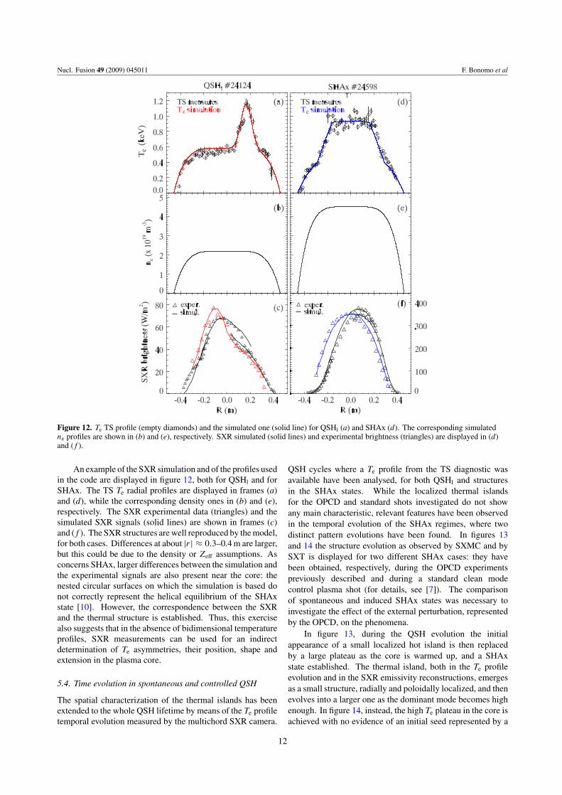
Figure 12. Te TS profile (empty diamonds) and the simulated one (solid line) for QSHl (a) and SHAx (d). The corresponding simulatedne profiles are shown in (b) and (e), respectively. SXR simulated (solid lines) and experimental brightness (triangles) are displayed in (d)and ( f ).

An example of the SXR simulation and of the profiles usedin the code are displayed in figure 12, both for QSHl and forSHAx. The TS Te radial profiles are displayed in frames (a)and (d), while the corresponding density ones in (b) and (e),respectively. The SXR experimental data (triangles) and thesimulated SXR signals (solid lines) are shown in frames (c)and ( f ). The SXR structures are well reproduced by the model,for both cases. Differences at about |r| ≈ 0.3–0.4 m are larger,but this could be due to the density or Zeff assumptions. Asconcerns SHAx, larger differences between the simulation andthe experimental signals are also present near the core: thenested circular surfaces on which the simulation is based donot correctly represent the helical equilibrium of the SHAxstate [10]. However, the correspondence between the SXRand the thermal structure is established. Thus, this exercisealso suggests that in the absence of bidimensional temperatureprofiles, SXR measurements can be used for an indirectdetermination of Te asymmetries, their position, shape andextension in the plasma core.

5.4. Time evolution in spontaneous and controlled QSH

The spatial characterization of the thermal islands has beenextended to the whole QSH lifetime by means of the Te profiletemporal evolution measured by the multichord SXR camera.

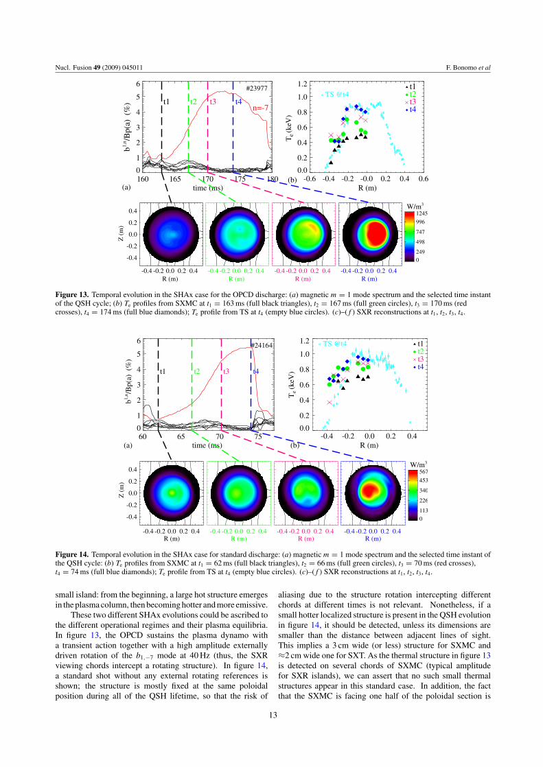
QSH cycles where a Te profile from the TS diagnostic wasavailable have been analysed, for both QSHl and structuresin the SHAx states. While the localized thermal islandsfor the OPCD and standard shots investigated do not showany main characteristic, relevant features have been observedin the temporal evolution of the SHAx regimes, where twodistinct pattern evolutions have been found. In figures 13and 14 the structure evolution as observed by SXMC and bySXT is displayed for two different SHAx cases: they havebeen obtained, respectively, during the OPCD experimentspreviously described and during a standard clean modecontrol plasma shot (for details, see [7]). The comparisonof spontaneous and induced SHAx states was necessary toinvestigate the effect of the external perturbation, representedby the OPCD, on the phenomena.

In figure 13, during the QSH evolution the initialappearance of a small localized hot island is then replacedby a large plateau as the core is warmed up, and a SHAxstate established. The thermal island, both in the Te profileevolution and in the SXR emissivity reconstructions, emergesas a small structure, radially and poloidally localized, and thenevolves into a larger one as the dominant mode becomes highenough. In figure 14, instead, the high Te plateau in the core isachieved with no evidence of an initial seed represented by a

12

Nucl. Fusion 49 (2009) 045011 F. Bonomo et al

-0.6 -0.4 -0.2 -0.0 0.2 0.4 0.6R (m)

0.0

0.2

0.4

0.6

0.8

1.0

1.2

Te (

keV

)

TS @t4t1t2t3t4

160 165 170 175 180time (ms)

0

1

2

3

4

5

6

b1,n /B

p(a)

(%

)

#23977

t1 t2 t3 t4n=-7

-0.4 -0.2 0.0 0.2 0.4R (m)

-0.4

-0.2

0.0

0.2

0.4

Z (

m)

-0.4 -0.2 0.0 0.2 0.4R (m)

-0.4 -0.2 0.0 0.2 0.4R (m)

-0.4 -0.2 0.0 0.2 0.4R (m)

W/m3

0249

498

747

996

1245

(a)(b)

Figure 13. Temporal evolution in the SHAx case for the OPCD discharge: (a) magnetic m = 1 mode spectrum and the selected time instantof the QSH cycle; (b) Te profiles from SXMC at t1 = 163 ms (full black triangles), t2 = 167 ms (full green circles), t3 = 170 ms (redcrosses), t4 = 174 ms (full blue diamonds); Te profile from TS at t4 (empty blue circles). (c)–( f ) SXR reconstructions at t1, t2, t3, t4.

-0.4 -0.2 0.0 0.2 0.4R (m)

0.0

0.2

0.4

0.6

0.8

1.0

1.2

Te (

keV

)

TS @t4 t1t2t3t4

60 65 70 75time (ms)

0

1

2

3

4

5

6

b1,n /B

p(a)

(%

)

#24164

t1 t2 t3 t4

-0.4 -0.2 0.0 0.2 0.4R (m)

-0.4

-0.2

0.0

0.2

0.4

Z (

m)

-0.4 -0.2 0.0 0.2 0.4R (m)

-0.4 -0.2 0.0 0.2 0.4R (m)

-0.4 -0.2 0.0 0.2 0.4R (m)

W/m3

0113

226

340

453

567

(a) (b)

Figure 14. Temporal evolution in the SHAx case for standard discharge: (a) magnetic m = 1 mode spectrum and the selected time instant ofthe QSH cycle: (b) Te profiles from SXMC at t1 = 62 ms (full black triangles), t2 = 66 ms (full green circles), t3 = 70 ms (red crosses),t4 = 74 ms (full blue diamonds); Te profile from TS at t4 (empty blue circles). (c)–( f ) SXR reconstructions at t1, t2, t3, t4.

small island: from the beginning, a large hot structure emergesin the plasma column, then becoming hotter and more emissive.

These two different SHAx evolutions could be ascribed tothe different operational regimes and their plasma equilibria.In figure 13, the OPCD sustains the plasma dynamo witha transient action together with a high amplitude externallydriven rotation of the b1,−7 mode at 40 Hz (thus, the SXRviewing chords intercept a rotating structure). In figure 14,a standard shot without any external rotating references isshown; the structure is mostly fixed at the same poloidalposition during all of the QSH lifetime, so that the risk of

aliasing due to the structure rotation intercepting differentchords at different times is not relevant. Nonetheless, if asmall hotter localized structure is present in the QSH evolutionin figure 14, it should be detected, unless its dimensions aresmaller than the distance between adjacent lines of sight.This implies a 3 cm wide (or less) structure for SXMC and≈2 cm wide one for SXT. As the thermal structure in figure 13is detected on several chords of SXMC (typical amplitudefor SXR islands), we can assert that no such small thermalstructures appear in this standard case. In addition, the factthat the SXMC is facing one half of the poloidal section is

13

Nucl. Fusion 49 (2009) 045011 F. Bonomo et al

a limit for our measurements, lacking Te information on theremaining ‘half’ QSH thermal structure evolution, but the2D SXR tomographic reconstructions do not show the presenceof small localized seeds at all.

Therefore, we can state that the evolution towards theSHAx regimes is not a unique process: in the OPCD, SHAxusually evolves from a small island, which is only theinitial stage. This does not happen during the standard caseconsidered here. Probably, a different plasma equilibriumcombined with a different evolution of the dominant andsecondary magnetic modes accounts for these differences; therelation of such a process with experimental conditions needsto be further investigated.

6. Summary and conclusions

The simultaneous availability of space and time resolved elec-tron temperature measurements in the RFX-mod experimenthas been used to characterize the topology of the QSH states,both in the presence of a localized QSHl structure and in theSHAx case. Dedicated experiments at Ip = 1.3–1.5 MA havebeen run: the temporal occurrence of the QSH structure hasbeen controlled through the OPCD technique, while its toroidaland poloidal positions have been varied through an externalrotating reference of the m = 1, n = −7 dominant mode.

Despite the unavailability of 2D electron temperaturemeasurements, such as on other fusion devices, a full 2D mapof the Te for localized QSHl and SHAx has been obtainedcombining the OPCD and the external rotating referencetechniques. A poloidal scan of the island Te profile has beendone varying the poloidal island O-point position and pulsingthe TS laser at the OPCD maximum. TS data have beenprocessed to obtain a 2D image of the localized bean-shapedthermal island in QSHl and of the large high Te plateau typicalof SHAx.

The TS Te profiles have been compared with thoseprovided by the SXR camera applying the island phase relationdescribed in equation (3). Further relevant information isalso provided by the tomographic reconstruction of the SXRemissivity profiles: the mutual agreement of the thermalstructure amplitudes and the SXR asymmetries is reportedhere, identifying the thermal structure with the SXR emissivityones. The flat density profiles and the constancy of Zeff permitone to conclude that in RFX-mod, the SXR structures areessentially driven by Te.

The transition to the SHAx state, with the plasma evolvingfrom the co-existence of a primary and a secondary magneticaxis to a helical equilibrium where the old axis has beenexpelled, has a substantial effect on the plasma Te profiles.The thermal width wTS and the magnetic amplitude wmag fromthe ORBIT code have been compared for the QSHl and SHAxcases: magnetic and thermal structures correspond in shape,dimension and position although a systematic difference couldbe explained by several approximations in the magnetic modelused. The island width, corresponding to the Te plateau inthe SHAx state, has a maximum extent of ≈45 cm decreasingto ≈30 cm as the island O-point position is exactly at 180◦ atthe TS location: the thermal plateau region is not poloidallysymmetric but still represents a relevant portion of the plasmacore (≈50%). For QSHl, the width weakly increases when

the O-point is near 180◦ at TS location, due to its bean-liketopology, up to ≈20 cm.

The larger plasma volume occupied by the SHAxstructure, with a high Te plateau, is associated with an increasein the global plasma performances. It has in fact been reportedin [31] that the electron energy confinement time τe,E increaseson average in SHAx with respect to the QSHl cases, withpeak values that are almost twice. The τe,E has been roughlyestimated by applying the µ&p axisymmetric equilibriummodel [32] for the determination of input power deposition.This is an unavoidable approximation, since the measurementof the power source inside the island is still an unresolvedissue: while the island grows and is heated up, the currentdensity profile is modified, but the latter is not measured onRFX-mod. Such an improved confinement assures a reductionof transport as estimated by different approaches, as can befound in [24, 33] or in [20].

While the transition to separatrix expulsion has beenpredicted and described by theory [34] in terms of theinitial and final states of a generic Hamiltonian system, itsdynamical evolution has never been considered so far. TheQSH temperature profile evolution during such a transitionconsists of at least two distinct processes. In one case, theappearance of a small localized hot island is then replacedby the large plateau which is then warmed up. In the othercase, a large hot structure emerges in the plasma column fromthe beginning. These two processes are related to two differentoperational methods presenting different plasma equilibria andmagnetic mode evolution and may represent a tool for furtherinvestigating the physical process for achieving the SH stateexperimentally.

Acknowledgments

This work was supported by the European Communities underthe contract of Association between EURATOM/ENEA. Theviews and opinions expressed herein do not necessarily reflectthose of the European Commission.

Appendix. Approximated absolute calibration of themain TS diagnostic

The electron density and temperature measurements fromthe main TS and the interferometer diagnostics are usuallycombined to get the electron pressure (pe) profile. Thisreconstruction is carried out by means of the poloidal map-ping of diagnostic view lines onto the magnetic mid-planeusing the magnetic equilibrium reconstruction, relying on theaccuracy of magnetic field surface reconstruction. However,the need for this mapping exercise is overcome in case themain TS system is absolutely calibrated, since in this casethe TS system measures profiles of Te and ne simultaneouslyin the plasma mid-plane. Electron density profiles measuredby the main TS diagnostic on RFX-mod are usually obtainedby absolutely calibrating the spectrometers with rotationalRaman scattering (RRS) in nitrogen: the amplitude of anti-Stokes RRS lines in N2 is monitored as a linear function ofpressure from 20 up to 150 mbar [16], and a calibration factoris calculated for each scattering volume. Nevertheless, each

14

Nucl. Fusion 49 (2009) 045011 F. Bonomo et al

absolute calibration is valid only for a limited series of a fewhundred shots as the maximum or even less if wall condition-ing discharges are performed (e.g. in boron or helium). Themain issue is represented by plasma deposition on the inter-nal face of the collection windows, which degrades the opticaltransmission of the collection windows and causes a slight dis-tortion of the spectral transmission curve. The modificationof the collection optics spectral response represents a threatto measurement accuracy since it decreases the signal ampli-tude and introduces systematic errors in data analysis. Whilethe effect on Te in RFX-mod is negligible [35], it seriouslyaffects the absolute calibration stability. To cope with thisproblem, the transmission of TS collection windows should beroutinely monitored by scanning the available internal dc lightsource along the scattering volume and, when required, theRaman calibration should be performed. For operative con-straints, this cannot be done, and the absolute calibration ishence not always available. An alternative solution has beenadopted to overcome this problem. Electron density profilesare flat in the core of RFX-mod during MH states, withoutany density structure being wider than the accuracy of themain TS system (10 mm): in this case, the absolute calibra-tion factors of core scattering volumes can be derived from acomparison with the density profile obtained from inversionof the interferometer measurements. A more approximativecross-calibration approach consists of calculating the calibra-tion factors from the relative variations to an analytical fit ofthe density profile in a MH plasma: the imposed density profileis ne(r) = ne,0 · (1 − (r/a)8)), where ne,0 is the core densityfrom the central cord of the interferometer diagnostic. Thislatter method is obviously too rough to study the edge region,where density gradients can vary in a wide range, but bothmethods are reliable for detecting the presence of core densitystructures along the TS temperature profile. Both have beenapplied to the plasma discharges used in this paper, and theyconfirm that the density profiles are flat in the core during theQSHl and SHAx states considered for the analysis.

CONSORZIO RFX–EURATOM/ENEA Association© 2009.

References

[1] Taylor J.B. 1974 Phys. Rev. Lett. 33 1139[2] Bonfiglio D., Cappello S. and Escande D.F. 2005 Phys. Rev.

Lett. 94 145001[3] Cappello S. et al 2008 Theory of fusion plasmas AIP Conf.

Proc. 1069 27–39[4] Martin P. et al and the RFX-mod team 2007 Plasma Phys.

Control. Fusion 49 A177[5] Sonato P. et al 2003 Fusion Eng. Des. 66–68 161–8[6] Zanca P., Marrelli L. and Manduchi G. 2007 Nucl. Fusion

47 1425[7] Marrelli L. et al 2007 Plasma Phys. Control. Fusion

49 B359

[8] Valisa M. and the RFX-mod Team 2008 Plasma Phys. Control.Fusion 50 124031

[9] Alfier A., Pasqualotto R., Spizzo G., Canton A., Fassina A.and Frassinetti L. 2008 Plasma Phys. Control. Fusion50 035013

[10] Lorenzini R., Terranova D., Alfier A., Innocente P.,Martines E., Roberto P. and Zanca P. 2008 Phys. Rev. Lett.101 025005

[11] Lichtenberg A.J. and Lieberman M.A. 1992 Regular andChaotic Dynamics 2nd edn (New York: Springer)

[12] Terranova D., Alfier A., Bonomo F., Franz P., Innocente P. andPasqualotto R. 2007 Phys. Rev. Lett. 99 095001

[13] Bonomo F., Franz P., Murari A., Gadani G., Alfier A. andPasqualotto R. 2006 Rev. Sci. Instrum. 77 10F313

[14] Donaldson T.P. 1978 Plasma Phys. 20 1279[15] Kiraly J. 1987 Nucl. Fusion 27 397[16] Alfier A. and Pasqualotto R. 2007 Rev. Sci. Instrum. 78 013505[17] Franz P., Marrelli L., Murari A., Spizzo G. and Martin P. 2001

Nucl. Fusion 41 695–709[18] Carraro L., Puiatti M.E., Sattin F., Scarin P., Valisa M. and

Mattioli M. 1996 Nucl. Fusion 36 1623[19] Carraro L. et al 2008 Proc. 35th EPS Conf. on Plasma Physics

(Crete, Greece, 9–13 June 2008) ECA vol 32D P4.019http://epsppd.epfl.ch/Hersonissos/pdf/P4 019.pdf/

[20] Annibaldi S.V., Bonomo F., Pasqualotto R., Spizzo G.,Alfier A., Buratti P., Piovesan P. and Terranova D. 2007Phys. Plasmas 14 112515

[21] Puiatti M.E. and the RFX-mod Team 2008 Proc. 22nd IAEAFusion Energy Conf. (Geneva, Switzerland, 13–18 October2008) EX/P5–22 http://www-pub.iaea.org/MTCD/Meetings/FEC2008/EX P5-22.pdf

[22] White R.B. and Chance M.S. 1984 Phys. Fluids 27 2455[23] Zanca P. and Terranova D. 2004 Plasma Phys. Control. Fusion

46 1115[24] Gobbin M. et al 2007 Proc. 34th EPS Conf. on Plasma Physics

(Warsaw, Poland, 2–6 July 2007) ECA vol 31F P1.107http://epsppd.epfl.ch/Warsaw/pdf/P1 107.pdf

[25] Franz P. et al 2006 Rev. Sci. Instrum. 77 10F318[26] Park H. et al 2004 Rev. Sci. Instrum. 75 3875[27] Innocente P., Martini S. and Schio A. 1990 Rev. Sci. Instrum.

61 2885[28] Gregoratto D., Garzotti L., Innocente P., Martini S. and

Canton A. 1998 Nucl. Fusion 38 1199[29] Lorenzini R., Terranova D., Auriemma F., Cavazzana R.,

Innocente P., Martini S., Serianni G. and Zuin M. 2007Nucl. Fusion 47 1468–75

[30] Wesson J.A. 1995 Plasma Phys. Control. Fusion 37 A337[31] Piovesan P. et al 2008 Proc. 35th EPS Conf. on Plasma

Physics (Hersonissos,Crete, 9–13 June 2008) ECA vol 32DO4.029 http://epsppd.epfl.ch/Hersonissos/pdf/O4 029.pdf

[32] Ortolani S. 1984 Proc. Int. School of Plasma Physics, Courseon Mirror-based and Field-reversed Approaches toMagnetic Fusion (Varenna, Italy, 1983) vol 2 ed G.G.Leotta et al (Citta di Castello: Franchi) p 513

[33] Gobbin M., Guo S.C., Cappello S., Sattin F., Marrelli L. andGarzotti L. 2008 Proc. 35th EPS Conf. on ControlledFusion and Plasma Physics (Hersonissos, Crete, 9–13 June2008) ECA vol 32D P5.035 http://epsppd.epfl.ch/Hersonissos/pdf/P5 035.pdf

[34] Escande D.F., Paccagnella R., Cappello S., D’Angelo F. andMarchetto C. 2000 Phys. Rev. Lett. 85 3169

[35] Alfier A., Barison S., Danieli T., Giudicotti L., Pagura C. andPasqualotto R. 2008 Rev. Sci. Instrum. 79 10F338

15