204456: Machine Learning - Ch02 - Maths refresher
41
. . . . . . . . . . . . . . . . . . . . . . . . . . . . . . . . . . . . . . . . 204456: Machine Learning Ch02 - Maths refresher Jakramate Bootkrajang Department of Computer Science Chiang Mai University Based on materials for CSS490 by Prof. Jeff Howbert Jakramate Bootkrajang 204456: Machine Learning 1 / 41
-
Upload
khangminh22 -
Category
Documents
-
view
0 -
download
0
Transcript of 204456: Machine Learning - Ch02 - Maths refresher

...
.
...
.
...
.
...
.
...
.
...
.
...
.
...
.
...
.
...
.
204456: Machine LearningCh02 - Maths refresher
Jakramate Bootkrajang
Department of Computer ScienceChiang Mai University
Based on materials for CSS490 by Prof. Jeff Howbert
Jakramate Bootkrajang 204456: Machine Learning 1 / 41

...
.
...
.
...
.
...
.
...
.
...
.
...
.
...
.
...
.
...
.
Objective
To look at essential maths concepts for this course Linear algebra
Statistics
Optimisation
Jakramate Bootkrajang 204456: Machine Learning 2 / 41

...
.
...
.
...
.
...
.
...
.
...
.
...
.
...
.
...
.
...
.
Area of maths essential to ML
Linear algebra A study of vector/matrix
Data in ML is represented in vector/matrix form
Statistics Some say ‘Machine learning is part of both statistics and CS’
Probability, statistical inference, validation
Optimisation theory The ‘learning’ part in machine learning
Rely hugely on calculus
Jakramate Bootkrajang 204456: Machine Learning 3 / 41

...
.
...
.
...
.
...
.
...
.
...
.
...
.
...
.
...
.
...
.
Why worry about the maths ?
You will know how to apply ML packages after this course
However to get really useful results, you need
to have good mathmatical intuition of ML principles
to understand the working of those algorithms so that know how to choose the right algorithm
know how to set hyper-parameters
troubleshoot poor results
Jakramate Bootkrajang 204456: Machine Learning 4 / 41

...
.
...
.
...
.
...
.
...
.
...
.
...
.
...
.
...
.
...
.
Notations
a ∈ A set membership: a is a member of set A|B| cardinality: number of items in set B||v|| norm: length of vector v∑
summation∫integral
R the set of real numberRd real number space of dimension d
Jakramate Bootkrajang 204456: Machine Learning 5 / 41

...
.
...
.
...
.
...
.
...
.
...
.
...
.
...
.
...
.
...
.
Notations
x,u, v vector (bold, lower case)X,B matrix (bold, upper case)y = f(x) function: assign unique value in set Y to each value in set Xdydx derivative of y with respect to single variable xy = f(x) function in d-space∂y∂xi
partial derivative of y with respect to element i of x
Jakramate Bootkrajang 204456: Machine Learning 6 / 41

...
.
...
.
...
.
...
.
...
.
...
.
...
.
...
.
...
.
...
.
Linear algebra
Jakramate Bootkrajang 204456: Machine Learning 7 / 41

...
.
...
.
...
.
...
.
...
.
...
.
...
.
...
.
...
.
...
.
Applications
Operations on or between vectors and matrices
Dimensionality reduction
Linear regression
Support Vector Machine
Jakramate Bootkrajang 204456: Machine Learning 8 / 41

...
.
...
.
...
.
...
.
...
.
...
.
...
.
...
.
...
.
...
.
Why vector and matrices ?
Most common form of data organisation for ML is 2D arry rows represent samples (datapoints)
columns represent attributes (features)
Natural to think of each sample as a vector of attributes and wholearray as a matrix
Jakramate Bootkrajang 204456: Machine Learning 9 / 41

...
.
...
.
...
.
...
.
...
.
...
.
...
.
...
.
...
.
...
.
Data matrix
Jakramate Bootkrajang 204456: Machine Learning 10 / 41
...
.
...
.
...
.
...
.
...
.
...
.
...
.
...
.
...
.
...
.
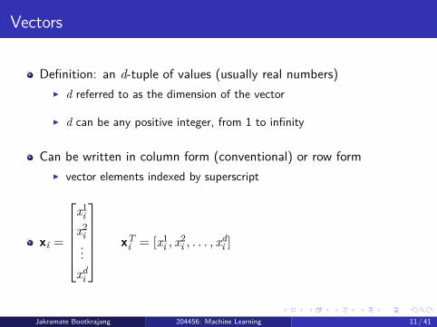
Vectors
Definition: an d-tuple of values (usually real numbers) d referred to as the dimension of the vector
d can be any positive integer, from 1 to infinity
Can be written in column form (conventional) or row form vector elements indexed by superscript
xi =
x1
ix2
i...
xdi
xTi = [x1
i , x2i , . . . , xd
i ]
Jakramate Bootkrajang 204456: Machine Learning 11 / 41

...
.
...
.
...
.
...
.
...
.
...
.
...
.
...
.
...
.
...
.
Vectors
can think of a vector as a point in space
Jakramate Bootkrajang 204456: Machine Learning 12 / 41

...
.
...
.
...
.
...
.
...
.
...
.
...
.
...
.
...
.
...
.
Vector arithmetic
Addition of two vectors add corresponding elements
z = x + y = (x1 + y1, · · · , xd + yd)T
result is a vector
Scalar multiplication multiply each element by scalar
y = ax = (ax1, · · · , axd)T
result is a vector
Jakramate Bootkrajang 204456: Machine Learning 13 / 41

...
.
...
.
...
.
...
.
...
.
...
.
...
.
...
.
...
.
...
.
Vector arithmetic
Dot product of two vectors multiply corresponding elements, then add products
a = x · y =∑d
i=1 xiyi
result is scalar
Jakramate Bootkrajang 204456: Machine Learning 14 / 41

...
.
...
.
...
.
...
.
...
.
...
.
...
.
...
.
...
.
...
.
Matrices
Definition: an n × d two-dimensional array of values (usually realnumbers)
n rows, d columns
Matrix referenced by two-element subscript first element in subscript is row
second element is column
A13 or a13 is element in the first row, third column of A
Jakramate Bootkrajang 204456: Machine Learning 15 / 41
...
.
...
.
...
.
...
.
...
.
...
.
...
.
...
.
...
.
...
.
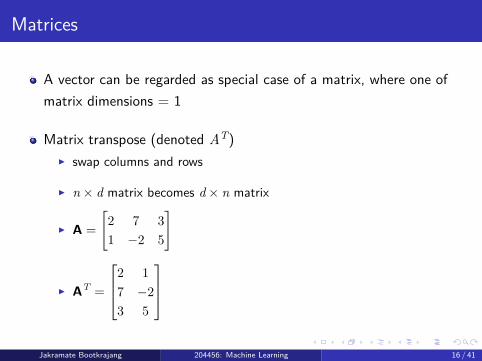
Matrices
A vector can be regarded as special case of a matrix, where one ofmatrix dimensions = 1
Matrix transpose (denoted AT) swap columns and rows
n × d matrix becomes d × n matrix
A =
[2 7 31 −2 5
]
AT =
2 17 −23 5
Jakramate Bootkrajang 204456: Machine Learning 16 / 41
...
.
...
.
...
.
...
.
...
.
...
.
...
.
...
.
...
.
...
.
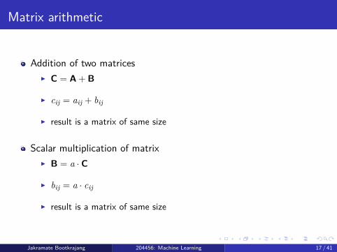
Matrix arithmetic
Addition of two matrices C = A + B
cij = aij + bij
result is a matrix of same size
Scalar multiplication of matrix B = a · C
bij = a · cij
result is a matrix of same size
Jakramate Bootkrajang 204456: Machine Learning 17 / 41

...
.
...
.
...
.
...
.
...
.
...
.
...
.
...
.
...
.
...
.
Matrix multiplication
TO THE BOARD
Multiplication is associative: A · (B · C) = (A · B) · C
Not commutative: A · B = B · A
Transposition rule: (AB)T = BTAT
Jakramate Bootkrajang 204456: Machine Learning 18 / 41

...
.
...
.
...
.
...
.
...
.
...
.
...
.
...
.
...
.
...
.
Matrix multiplication
RULE: In any chain of matrix multiplications, the column dimensionof one matrix in the chain must match the row dimension of thefollowing matrix in the chain.
Example: A 3 × 5, B 5 × 5, C 3 × 1
Right: A · B · AT
Wrong: C · A · B
Jakramate Bootkrajang 204456: Machine Learning 19 / 41

...
.
...
.
...
.
...
.
...
.
...
.
...
.
...
.
...
.
...
.
Statistics
Jakramate Bootkrajang 204456: Machine Learning 20 / 41

...
.
...
.
...
.
...
.
...
.
...
.
...
.
...
.
...
.
...
.
Concept of probability
In some process, several outcomes are possible. When the process isrepeated a large number of times, each outcome occurs with a
characteristic relative frequency or probability. If a outcome happens moreoften than another outcome we say it is more probable.
Jakramate Bootkrajang 204456: Machine Learning 21 / 41

...
.
...
.
...
.
...
.
...
.
...
.
...
.
...
.
...
.
...
.
Probability spaces
A probability space is a random process or experiment with threecomponents:
Ω, the set of possible outcomes⋆ number of possible outcomes = |Ω| = N
F, the set of possible events E⋆ an event comprises 0 to N outcomes⋆ think of as a dichotomy of outcomes⋆ number of possible events = |F| = 2N
P, the probability distribution⋆ function mapping each outcome and event to real number between 0
and 1
Jakramate Bootkrajang 204456: Machine Learning 22 / 41

...
.
...
.
...
.
...
.
...
.
...
.
...
.
...
.
...
.
...
.
Axioms of probability
1 Non-negativity p(E) ≥ 0 for all E ∈ F
2 All possible outcomes p(Ω) = 1
3 Additivity of disjoint events: for all events E,E′ ∈ F whereE ∩ E′ = ∅, p(E ∪ E′) = p(E) + p(E′)
Jakramate Bootkrajang 204456: Machine Learning 23 / 41
...
.
...
.
...
.
...
.
...
.
...
.
...
.
...
.
...
.
...
.
Types of probability spaces
Discrete space |Ω| is finite
Continuous space |Ω| is infinite
Jakramate Bootkrajang 204456: Machine Learning 24 / 41

...
.
...
.
...
.
...
.
...
.
...
.
...
.
...
.
...
.
...
.
Example of discrete probability space
Single roll of a six-sided die (singular of dice)6 possible outcomes: O = 1, 2, 3, 4, 5, 6
26 = 64 possible events E = O ∈ 1, 3, 5 outcome is odd
If die if fair, p(1) = p(2) = p(3) = p(4) = p(5) = p(6) = 1/6
Jakramate Bootkrajang 204456: Machine Learning 25 / 41
...
.
...
.
...
.
...
.
...
.
...
.
...
.
...
.
...
.
...
.
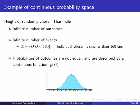
Example of continuous probability space
Height of randomly chosen Thai maleInfinite number of outcomes
Infinite number of events E = O|O < 160 individual chosen is smaller than 160 cm.
Probabilities of outcomes are not equal, and are described by acontinuous function, p(O)
Jakramate Bootkrajang 204456: Machine Learning 26 / 41

...
.
...
.
...
.
...
.
...
.
...
.
...
.
...
.
...
.
...
.
Example of continuous probability space
Height of randomly chosen Thai male
p(O) is relative not absolute
p(O = 175) = 0
but we can still make comparison p(O = 170) > p(O = 180) ?
Jakramate Bootkrajang 204456: Machine Learning 27 / 41

...
.
...
.
...
.
...
.
...
.
...
.
...
.
...
.
...
.
...
.
Random variables
A random variable X is a function that associates a number (label) xwith each outcome O of a process
Basically a way to redefine (usually simplify) a probability space to anew probability space
Example X = number of heads in three coin flips possible values of X are 0,1,2,3
Example X = region of car manufacturer Original outcomes could be a set of countries
possible values of X are 1=European, 2=Asia, 3=America
Jakramate Bootkrajang 204456: Machine Learning 28 / 41

...
.
...
.
...
.
...
.
...
.
...
.
...
.
...
.
...
.
...
.
Multivariate probability distribution
Scenario Several random processes occur
Want to know probabilities for each possible combination of outcomes.
Can describe as joint probability of random variables two processes whose outcomes are represented by random variables X
and Y, Probability that process X has outcome x and process Y hasoutcome y is denoted as: p(X = x,Y = y)
Jakramate Bootkrajang 204456: Machine Learning 29 / 41

...
.
...
.
...
.
...
.
...
.
...
.
...
.
...
.
...
.
...
.
Example of multivariate distribution
Jakramate Bootkrajang 204456: Machine Learning 30 / 41

...
.
...
.
...
.
...
.
...
.
...
.
...
.
...
.
...
.
...
.
Multivariate probability distributionMarginal probability
Probability distribution of a single variable in a joint distribution
p(X = x) =∑
y p(X = x,Y = y)
Jakramate Bootkrajang 204456: Machine Learning 31 / 41

...
.
...
.
...
.
...
.
...
.
...
.
...
.
...
.
...
.
...
.
Multivariate probability distribution
Conditional probability Probability distribution of one variable given that another variable
takes a certain value
p(X = x|Y = y) = p(X = x,Y = y)/p(Y = y)
Jakramate Bootkrajang 204456: Machine Learning 32 / 41

...
.
...
.
...
.
...
.
...
.
...
.
...
.
...
.
...
.
...
.
Continuous probability distribution
Same concepts of joint, marginal, and conditional probabilities apply(except use integrals)
Jakramate Bootkrajang 204456: Machine Learning 33 / 41

...
.
...
.
...
.
...
.
...
.
...
.
...
.
...
.
...
.
...
.
Expected value
GivenA discrete random variable X, with possible values x = x1, x2, . . . , xn
Probability p(X = xi)
A function yi = f(xi) defined on XExpected value is the probability-weighted “average” of f(xi)
E(f) =∑
ip(xi) · f(xi) (1)
Jakramate Bootkrajang 204456: Machine Learning 34 / 41
...
.
...
.
...
.
...
.
...
.
...
.
...
.
...
.
...
.
...
.
Calculus
Jakramate Bootkrajang 204456: Machine Learning 35 / 41

...
.
...
.
...
.
...
.
...
.
...
.
...
.
...
.
...
.
...
.
Derivative
A derivative of function at x0 is the rate of change of function values asinput changes near x0
dydx =
df(xo)
dx = limh→0
f(x0 + h)− f(x0)
h
Jakramate Bootkrajang 204456: Machine Learning 36 / 41
...
.
...
.
...
.
...
.
...
.
...
.
...
.
...
.
...
.
...
.
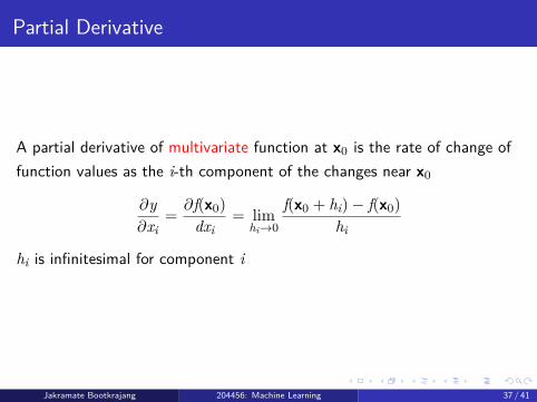
Partial Derivative
A partial derivative of multivariate function at x0 is the rate of change offunction values as the i-th component of the changes near x0
∂y∂xi
=∂f(x0)
dxi= lim
hi→0
f(x0 + hi)− f(x0)
hi
hi is infinitesimal for component i
Jakramate Bootkrajang 204456: Machine Learning 37 / 41

...
.
...
.
...
.
...
.
...
.
...
.
...
.
...
.
...
.
...
.
Common derivatives
daf(x)dx = adf(x)
dx
dxk
dx = kxk−1
df(x)+g(x)dx = df(x)
dx + dg(x)dx
df(x)g(x)dx = f(x)dg(x)
dx + g(x)df(x)dx
dex
dx = ex
d log(x)dx = 1
x
Jakramate Bootkrajang 204456: Machine Learning 38 / 41

...
.
...
.
...
.
...
.
...
.
...
.
...
.
...
.
...
.
...
.
Gradient
A vector of partial derivatives
∇f(x) =
∂f(x)dx1∂f(x)dx2...∂f(x)dxd
Jakramate Bootkrajang 204456: Machine Learning 39 / 41

...
.
...
.
...
.
...
.
...
.
...
.
...
.
...
.
...
.
...
.
Hessian
A matrix of second partial derivatives
Jakramate Bootkrajang 204456: Machine Learning 40 / 41
...
.
...
.
...
.
...
.
...
.
...
.
...
.
...
.
...
.
...
.
References
Math for Machine learning by Hal Daume III http://users.umiacs.umd.edu/~hal/courses/2013S_ML/math4ml.pdf
Machine learning math essentials by Jeff Howberthttp://courses.washington.edu/css490/2012.Winter/lecture_slides/02_math_essentials.pdf
Jakramate Bootkrajang 204456: Machine Learning 41 / 41