Everything Maths Grade 11
238
Transcript of Everything Maths Grade 11


Everything Maths
Grade 11 Mathematics
Version 0.9 – NCS
by Siyavula and volunteers

Copyright notice
Your freedom to legally copy this book
You are allowed and encouraged to freely copy this book. You can photocopy, print anddistribute it as often as you like. You can download it onto your mobile phone, iPad, PC orflash drive. You can burn it to CD, e-mail it around or upload it to your website.
The only restriction is that you have to keep this book, its cover and short-codes unchanged.
For more information about the Creative Commons Attribution-NoDerivs 3.0 Unported (CCBY-ND 3.0) license see http://creativecommons.org/licenses/by-nd/3.0/

Authors List
This book is based upon the original Free High School Science Text which was entirely writtenby volunteer academics, educators and industry professionals. Their vision was to see a cur-riculum aligned set of mathematics and physical science textbooks which are freely availableto anybody and exist under an open copyright license.
Siyavula core team
Neels van der Westhuizen; Alison Jenkin; Marina van Zyl; Helen Robertson; Carl Scheffler; Nicola du Toit; Leonard Gumani
Mudau;
Original Free High School Science Texts core team
Mark Horner; Samuel Halliday; Sarah Blyth; Rory Adams; Spencer Wheaton
Original Free High School Science Texts editors
Jaynie Padayachee; Joanne Boulle; Diana Mulcahy; Annette Nell; Ren Toerien; Donovan Whitfield
Siyavula and Free High School Science Texts contributors
Sarah Abel; Dr. Rory Adams; Andrea Africa; Matthew Amundsen; Ben Anhalt; Prashant Arora; Amos Baloyi; Bongani Baloyi;
Raymond Barbour; Caro-Joy Barendse; Richard Baxter; Tara Beckerling; Dr. Sarah Blyth; Sebastian Bodenstein; Martin Bongers;
Gareth Boxall; Stephan Brandt; Hannes Breytenbach; Alex Briell; Wilbur Britz; Graeme Broster; Craig Brown; Richard Burge;
Bianca Bhmer; George Calder-Potts; Eleanor Cameron; Richard Case; Sithembile Cele; Alice Chang; Richard Cheng; Fanny
Cherblanc; Dr. Christine Chung; Brett Cocks; Stefaan Conradie; Rocco Coppejans; Tim Craib; Andrew Craig; Tim Crombie;
Dan Crytser; Dr. Anne Dabrowski; Laura Daniels; Gareth Davies; Jennifer de Beyer; Jennifer de Beyer; Deanne de Bude; Mia
de Vos; Sean Dobbs; Buhle Donga; William Donkin; Esmi Dreyer; Nicola du Toit; Matthew Duddy; Fernando Durrell; Dr.
Dan Dwyer; Alex Ellis; Tom Ellis; Andrew Fisher; Giovanni Franzoni; Nina Gitau Muchunu; Lindsay Glesener; Kevin Godby;
Dr. Vanessa Godfrey; Terence Goldberg; Dr. Johan Gonzalez; Saaligha Gool; Hemant Gopal; Dr. Stephanie Gould; Umeshree
Govender; Heather Gray; Lynn Greeff; Carine Grobbelaar; Dr. Tom Gutierrez; Brooke Haag; Kate Hadley; Alex Hall; Dr. Sam
Halliday; Asheena Hanuman; Dr. Nicholas Harrison; Neil Hart; Nicholas Hatcher; Jason Hayden; Laura Hayward; Cho Hee
Shrader; Dr. Fritha Hennessy; Shaun Hewitson; Millie Hilgart; Grant Hillebrand; Nick Hobbs; Chris Holdsworth; Dr. Benne
Holwerda; Dr. Mark Horner; Robert Hovden; Mfandaidza Hove; Jennifer Hsieh; Laura Huss; Dr. Matina J. Rassias; Rowan
Jelley; Grant Jelley; Clare Johnson; Luke Jordan; Tana Joseph; Dr. Fabian Jutz; Brian Kamanzi; Dr. Lutz Kampmann; Simon
Katende; Natalia Kavalenia; Nothando Khumalo; Paul Kim; Dr. Jennifer Klay; Lara Kruger; Sihle Kubheka; Andrew Kubik;
Dr. Jannie Leach; Nkoana Lebaka; Dr. Tom Leinster; Henry Liu; Christopher Loetscher; Mike Loseby; Amandla Mabona;
Malothe Mabutho; Stuart Macdonald; Dr. Anton Machacek; Tshepo Madisha; Batsirai Magunje; Dr. Komal Maheshwari;
Michael Malahe; Masoabi Malunga; Masilo Mapaila; Bryony Martin; Nicole Masureik; John Mathew; Dr. Will Matthews;
Chiedza Matuso; JoEllen McBride; Dr Melanie Dymond Harper; Nikolai Meures; Riana Meyer; Filippo Miatto; Jenny Miller;
Abdul Mirza; Mapholo Modise; Carla Moerdyk; Tshwarelo Mohlala; Relebohile Molaoa; Marasi Monyau; Asogan Moodaly;
Jothi Moodley; Robert Moon; Calvin Moore; Bhavani Morarjee; Kholofelo Moyaba; Kate Murphy; Emmanuel Musonza; Tom
Mutabazi; David Myburgh; Kamie Naidu; Nolene Naidu; Gokul Nair; Vafa Naraghi; Bridget Nash; Tyrone Negus; Huw
Newton-Hill; Buntu Ngcebetsha; Dr. Markus Oldenburg; Thomas ODonnell; Dr. William P. Heal; Dr. Jaynie Padayachee;
Poveshen Padayachee; Masimba Paradza; Dave Pawson; Justin Pead; Nicolette Pekeur; Sirika Pillay; Jacques Plaut; Barry
Povey; Barry Povey; Andrea Prinsloo; Joseph Raimondo; Sanya Rajani; Alastair Ramlakan; Dr. Jocelyn Read; Jonathan Reader;
Jane Reddick; Dr. Matthew Reece; Razvan Remsing; Laura Richter; Max Richter; Sean Riddle; Dr. David Roberts; Christopher
Roberts; Helen Robertson; Evan Robinson; Raoul Rontsch; Dr. Andrew Rose; Katie Ross; Jeanne-Mari Roux; Mark Roux;
Bianca Ruddy; Nitin Rughoonauth; Katie Russell; Steven Sam; Dr. Carl Scheffler; Nathaniel Schwartz; Duncan Scott; Helen
Seals; Relebohile Sefako; Prof. Sergey Rakityansky; Sandra Serumaga-Zake; Paul Shangase; Cameron Sharp; Ian Sherratt; Dr.
James Short; Roger Sieloff; Brandon Sim; Bonga Skozana; Clare Slotow; Bradley Smith; Greg Solomon; Nicholas Spaull; Dr.
Andrew Stacey; Dr. Jim Stasheff; Mike Stay; Mike Stringer; Masixole Swartbooi; Tshenolo Tau; Tim Teatro; Ben Tho.epson;
Shen Tian; Xolani Timbile; Robert Torregrosa; Jimmy Tseng; Tim van Beek; Neels van der Westhuizen; Frans van Eeden; Pierre
van Heerden; Dr. Marco van Leeuwen; Marina van Zyl; Pieter Vergeer; Rizmari Versfeld; Mfundo Vezi; Mpilonhle Vilakazi;
Ingrid von Glehn; Tamara von Glehn; Kosma von Maltitz; Helen Waugh; Leandra Webb; Dr. Dawn Webber; Michelle Wen;
Dr. Alexander Wetzler; Dr. Spencer Wheaton; Vivian White; Dr. Gerald Wigger; Harry Wiggins; Heather Williams; Wendy
Williams; Julie Wilson; Timothy Wilson; Andrew Wood; Emma Wormauld; Dr. Sahal Yacoob; Jean Youssef; Ewald Zietsman

Everything MathsMathematics is commonly thought of as being about numbers but mathematics is actually a language!
Mathematics is the language that nature speaks to us in. As we learn to understand and speak this lan-
guage, we can discover many of nature’s secrets. Just as understanding someone’s language is necessary
to learn more about them, mathematics is required to learn about all aspects of the world – whether it
is physical sciences, life sciences or even finance and economics.
The great writers and poets of the world have the ability to draw on words and put them together in ways
that can tell beautiful or inspiring stories. In a similar way, one can draw on mathematics to explain and
create new things. Many of the modern technologies that have enriched our lives are greatly dependent
on mathematics. DVDs, Google searches, bank cards with PIN numbers are just some examples. And
just as words were not created specifically to tell a story but their existence enabled stories to be told, so
the mathematics used to create these technologies was not developed for its own sake, but was available
to be drawn on when the time for its application was right.
There is in fact not an area of life that is not affected by mathematics. Many of the most sought after
careers depend on the use of mathematics. Civil engineers use mathematics to determine how to best
design new structures; economists use mathematics to describe and predict how the economy will react
to certain changes; investors use mathematics to price certain types of shares or calculate how risky
particular investments are; software developers use mathematics for many of the algorithms (such as
Google searches and data security) that make programmes useful.
But, even in our daily lives mathematics is everywhere – in our use of distance, time and money.
Mathematics is even present in art, design and music as it informs proportions and musical tones. The
greater our ability to understand mathematics, the greater our ability to appreciate beauty and everything
in nature. Far from being just a cold and abstract discipline, mathematics embodies logic, symmetry,
harmony and technological progress. More than any other language, mathematics is everywhere and
universal in its application.
See introductory video by Dr. Mark Horner: VMiwd at www.everythingmaths.co.za

More than a regular textbook
Everything Maths is not just a Mathematics textbook. It has everything you expect from your regular
printed school textbook, but comes with a whole lot more. For a start, you can download or read it
on-line on your mobile phone, computer or iPad, which means you have the convenience of accessing
it wherever you are.
We know that some things are hard to explain in words. That is why every chapter comes with video
lessons and explanations which help bring the ideas and concepts to life. Summary presentations at
the end of every chapter offer an overview of the content covered, with key points highlighted for easy
revision.
All the exercises inside the book link to a service where you can get more practice, see the full solution
or test your skills level on mobile and PC.
We are interested in what you think, wonder about or struggle with as you read through the book and
attempt the exercises. That is why we made it possible for you to use your mobile phone or computer
to digitally pin your question to a page and see what questions and answers other readers pinned up.

Everything Maths on your mobile or PCYou can have this textbook at hand wherever you are – whether at home, on the the train or at school.
Just browse to the on-line version of Everything Maths on your mobile phone, tablet or computer. To
read it off-line you can download a PDF or e-book version.
To read or download it, go to www.everythingmaths.co.za on your phone or computer.
Using the icons and short-codesInside the book you will find these icons to help you spot where videos, presentations, practice tools
and more help exist. The short-codes next to the icons allow you to navigate directly to the resources
on-line without having to search for them.
(A123) Go directly to a section
(V123) Video, simulation or presentation
(P123) Practice and test your skills
(Q123) Ask for help or find an answer
To watch the videos on-line, practise your skills or post a question, go to the Everything Maths website
at www.everythingmaths.co.za on your mobile or PC and enter the short-code in the navigation box.

Video lessonsLook out for the video icons inside the book. These will take you to video lessons that help bring the
ideas and concepts on the page to life. Get extra insight, detailed explanations and worked examples.
See the concepts in action and hear real people talk about how they use maths and science in their
work.
See video explanation (Video: V123)
Video exercisesWherever there are exercises in the book you will see icons and short-codes for video solutions, practice
and help. These short-codes will take you to video solutions of select exercises to show you step-by-step
how to solve such problems.
See video exercise (Video: V123)

You can get these videos by:
• viewing them on-line on your mobile or computer
• downloading the videos for off-line viewing on your phone or computer
• ordering a DVD to play on your TV or computer
• downloading them off-line over Bluetooth or Wi-Fi from select outlets
To view, download, or for more information, visit the Everything Maths website on your phone or
computer at www.everythingmaths.co.za
Practice and test your skillsOne of the best ways to prepare for your tests and exams is to practice answering the same kind of
questions you will be tested on. At every set of exercises you will see a practice icon and short-code.
This on-line practice for mobile and PC will keep track of your performance and progress, give you
feedback on areas which require more attention and suggest which sections or videos to look at.
See more practice (QM123)
To practice and test your skills:
Go to www.everythingmaths.co.za on your mobile phone or PC and enter the short-code.

Answers to your questionsHave you ever had a question about a specific fact, formula or exercise in your textbook and wished
you could just ask someone? Surely someone else in the country must have had the same question at
the same place in the textbook.
Database of questions and answers
We invite you to browse our database of questions and answer for every sections and exercises in the
book. Find the short-code for the section or exercise where you have a question and enter it into the
short-code search box on the web or mobi-site at www.everythingmaths.co.za or
www.everythingscience.co.za. You will be directed to all the questions previously asked and answered
for that section or exercise.
(A123) Visit this section to post or view questions
(Q123) Questions or help with a specific question
Ask an expert
Can’t find your question or the answer to it in the questions database? Then we invite you to try our
service where you can send your question directly to an expert who will reply with an answer. Again,
use the short-code for the section or exercise in the book to identify your problem area.

Contents
1 Introduction to the Book 2
1.1 The Language of Mathematics . . . . . . . . . . . . . . . . . . . . . . . . . . . . . . . . . . . . . . . . . . . . 2
2 Exponents 3
2.1 Introduction . . . . . . . . . . . . . . . . . . . . . . . . . . . . . . . . . . . . . . . . . . . . . . . . . . . . . 3
2.2 Laws of Exponents . . . . . . . . . . . . . . . . . . . . . . . . . . . . . . . . . . . . . . . . . . . . . . . . . . 3
2.3 Exponentials in the Real World . . . . . . . . . . . . . . . . . . . . . . . . . . . . . . . . . . . . . . . . . . . 6
3 Surds 9
3.1 Introduction . . . . . . . . . . . . . . . . . . . . . . . . . . . . . . . . . . . . . . . . . . . . . . . . . . . . . 9
3.2 Surd Calculations . . . . . . . . . . . . . . . . . . . . . . . . . . . . . . . . . . . . . . . . . . . . . . . . . . 9
4 Error Margins 18
4.1 Introduction . . . . . . . . . . . . . . . . . . . . . . . . . . . . . . . . . . . . . . . . . . . . . . . . . . . . . 18
4.2 Rounding Off . . . . . . . . . . . . . . . . . . . . . . . . . . . . . . . . . . . . . . . . . . . . . . . . . . . . 18
5 Quadratic Sequences 22
5.1 Introduction . . . . . . . . . . . . . . . . . . . . . . . . . . . . . . . . . . . . . . . . . . . . . . . . . . . . . 22
5.2 What is a Quadratic Sequence? . . . . . . . . . . . . . . . . . . . . . . . . . . . . . . . . . . . . . . . . . . . 22
6 Finance 30
6.1 Introduction . . . . . . . . . . . . . . . . . . . . . . . . . . . . . . . . . . . . . . . . . . . . . . . . . . . . . 30
6.2 Depreciation . . . . . . . . . . . . . . . . . . . . . . . . . . . . . . . . . . . . . . . . . . . . . . . . . . . . . 30
6.3 Simple Decay or Straight-line depreciation . . . . . . . . . . . . . . . . . . . . . . . . . . . . . . . . . . . . . 31
6.4 Compound Decay or Reducing-balance depreciation . . . . . . . . . . . . . . . . . . . . . . . . . . . . . . . 34
6.5 Present and Future Values of an Investment or Loan . . . . . . . . . . . . . . . . . . . . . . . . . . . . . . . . 37
6.6 Finding i . . . . . . . . . . . . . . . . . . . . . . . . . . . . . . . . . . . . . . . . . . . . . . . . . . . . . . . 38
6.7 Finding n — Trial and Error . . . . . . . . . . . . . . . . . . . . . . . . . . . . . . . . . . . . . . . . . . . . . 40
6.8 Nominal and Effective Interest Rates . . . . . . . . . . . . . . . . . . . . . . . . . . . . . . . . . . . . . . . . 41
6.9 Formula Sheet . . . . . . . . . . . . . . . . . . . . . . . . . . . . . . . . . . . . . . . . . . . . . . . . . . . . 46
7 Solving Quadratic Equations 49
7.1 Introduction . . . . . . . . . . . . . . . . . . . . . . . . . . . . . . . . . . . . . . . . . . . . . . . . . . . . . 49
7.2 Solution by Factorisation . . . . . . . . . . . . . . . . . . . . . . . . . . . . . . . . . . . . . . . . . . . . . . 49
7.3 Solution by Completing the Square . . . . . . . . . . . . . . . . . . . . . . . . . . . . . . . . . . . . . . . . . 53
7.4 Solution by the Quadratic Formula . . . . . . . . . . . . . . . . . . . . . . . . . . . . . . . . . . . . . . . . . 56
7.5 Finding an Equation When You Know its Roots . . . . . . . . . . . . . . . . . . . . . . . . . . . . . . . . . . . 61
8 Solving Quadratic Inequalities 66
8.1 Introduction . . . . . . . . . . . . . . . . . . . . . . . . . . . . . . . . . . . . . . . . . . . . . . . . . . . . . 66
8.2 Quadratic Inequalities . . . . . . . . . . . . . . . . . . . . . . . . . . . . . . . . . . . . . . . . . . . . . . . . 66
12

CONTENTS CONTENTS
9 Solving Simultaneous Equations 72
9.1 Introduction . . . . . . . . . . . . . . . . . . . . . . . . . . . . . . . . . . . . . . . . . . . . . . . . . . . . . 72
9.2 Graphical Solution . . . . . . . . . . . . . . . . . . . . . . . . . . . . . . . . . . . . . . . . . . . . . . . . . . 72
9.3 Algebraic Solution . . . . . . . . . . . . . . . . . . . . . . . . . . . . . . . . . . . . . . . . . . . . . . . . . . 74
10 Mathematical Models 78
10.1 Introduction . . . . . . . . . . . . . . . . . . . . . . . . . . . . . . . . . . . . . . . . . . . . . . . . . . . . . 78
10.2 Mathematical Models . . . . . . . . . . . . . . . . . . . . . . . . . . . . . . . . . . . . . . . . . . . . . . . . 78
10.3 Real-World Applications . . . . . . . . . . . . . . . . . . . . . . . . . . . . . . . . . . . . . . . . . . . . . . . 79
11 Quadratic Functions and Graphs 87
11.1 Introduction . . . . . . . . . . . . . . . . . . . . . . . . . . . . . . . . . . . . . . . . . . . . . . . . . . . . . 87
11.2 Functions of the Form y = a(x+ p)2 + q . . . . . . . . . . . . . . . . . . . . . . . . . . . . . . . . . . . . . . 87
12 Hyperbolic Functions and Graphs 96
12.1 Introduction . . . . . . . . . . . . . . . . . . . . . . . . . . . . . . . . . . . . . . . . . . . . . . . . . . . . . 96
12.2 Functions of the Form y = ax+p
+ q . . . . . . . . . . . . . . . . . . . . . . . . . . . . . . . . . . . . . . . . . 96
13 Exponential Functions and Graphs 103
13.1 Introduction . . . . . . . . . . . . . . . . . . . . . . . . . . . . . . . . . . . . . . . . . . . . . . . . . . . . . 103
13.2 Functions of the Form y = ab(x+p) + q for b > 0 . . . . . . . . . . . . . . . . . . . . . . . . . . . . . . . . . . 103
14 Gradient at a Point 109
14.1 Introduction . . . . . . . . . . . . . . . . . . . . . . . . . . . . . . . . . . . . . . . . . . . . . . . . . . . . . 109
14.2 Average Gradient . . . . . . . . . . . . . . . . . . . . . . . . . . . . . . . . . . . . . . . . . . . . . . . . . . 109
15 Linear Programming 113
15.1 Introduction . . . . . . . . . . . . . . . . . . . . . . . . . . . . . . . . . . . . . . . . . . . . . . . . . . . . . 113
15.2 Terminology . . . . . . . . . . . . . . . . . . . . . . . . . . . . . . . . . . . . . . . . . . . . . . . . . . . . . 113
15.3 Example of a Problem . . . . . . . . . . . . . . . . . . . . . . . . . . . . . . . . . . . . . . . . . . . . . . . . 115
15.4 Method of Linear Programming . . . . . . . . . . . . . . . . . . . . . . . . . . . . . . . . . . . . . . . . . . . 115
15.5 Skills You Will Need . . . . . . . . . . . . . . . . . . . . . . . . . . . . . . . . . . . . . . . . . . . . . . . . . 116
16 Geometry 127
16.1 Introduction . . . . . . . . . . . . . . . . . . . . . . . . . . . . . . . . . . . . . . . . . . . . . . . . . . . . . 127
16.2 Right Pyramids, Right Cones and Spheres . . . . . . . . . . . . . . . . . . . . . . . . . . . . . . . . . . . . . 127
16.3 Similarity of Polygons . . . . . . . . . . . . . . . . . . . . . . . . . . . . . . . . . . . . . . . . . . . . . . . . 131
16.4 Triangle Geometry . . . . . . . . . . . . . . . . . . . . . . . . . . . . . . . . . . . . . . . . . . . . . . . . . . 133
16.5 Co-ordinate Geometry . . . . . . . . . . . . . . . . . . . . . . . . . . . . . . . . . . . . . . . . . . . . . . . . 142
16.6 Transformations . . . . . . . . . . . . . . . . . . . . . . . . . . . . . . . . . . . . . . . . . . . . . . . . . . . 147
17 Trigonometry 154
17.1 Introduction . . . . . . . . . . . . . . . . . . . . . . . . . . . . . . . . . . . . . . . . . . . . . . . . . . . . . 154
17.2 Graphs of Trigonometric Functions . . . . . . . . . . . . . . . . . . . . . . . . . . . . . . . . . . . . . . . . . 154
17.3 Trigonometric Identities . . . . . . . . . . . . . . . . . . . . . . . . . . . . . . . . . . . . . . . . . . . . . . . 163
17.4 Solving Trigonometric Equations . . . . . . . . . . . . . . . . . . . . . . . . . . . . . . . . . . . . . . . . . . 175
17.5 Sine and Cosine Identities . . . . . . . . . . . . . . . . . . . . . . . . . . . . . . . . . . . . . . . . . . . . . . 188
13

CONTENTS CONTENTS
18 Statistics 198
18.1 Introduction . . . . . . . . . . . . . . . . . . . . . . . . . . . . . . . . . . . . . . . . . . . . . . . . . . . . . 198
18.2 Standard Deviation and Variance . . . . . . . . . . . . . . . . . . . . . . . . . . . . . . . . . . . . . . . . . . 198
18.3 Graphical Representation of Measures of Central Tendency and Dispersion . . . . . . . . . . . . . . . . . . . 204
18.4 Distribution of Data . . . . . . . . . . . . . . . . . . . . . . . . . . . . . . . . . . . . . . . . . . . . . . . . . 208
18.5 Scatter Plots . . . . . . . . . . . . . . . . . . . . . . . . . . . . . . . . . . . . . . . . . . . . . . . . . . . . . 210
18.6 Misuse of Statistics . . . . . . . . . . . . . . . . . . . . . . . . . . . . . . . . . . . . . . . . . . . . . . . . . . 213
19 Independent and Dependent Events 218
19.1 Introduction . . . . . . . . . . . . . . . . . . . . . . . . . . . . . . . . . . . . . . . . . . . . . . . . . . . . . 218
19.2 Definitions . . . . . . . . . . . . . . . . . . . . . . . . . . . . . . . . . . . . . . . . . . . . . . . . . . . . . . 218
1

Introduction to the Book 1
1.1 The Language of Mathematics EMBA
The purpose of any language, like English or Zulu, is to make it possible for people to communicate.
All languages have an alphabet, which is a group of letters that are used to make up words. There are
also rules of grammar which explain how words are supposed to be used to build up sentences. This
is needed because when a sentence is written, the person reading the sentence understands exactly
what the writer is trying to explain. Punctuation marks (like a full stop or a comma) are used to further
clarify what is written.
Mathematics is a language, specifically it is the language of Science. Like any language, mathematics
has letters (known as numbers) that are used to make up words (known as expressions), and sentences
(known as equations). The punctuation marks of mathematics are the different signs and symbols that
are used, for example, the plus sign (+), the minus sign (−), the multiplication sign (×), the equals sign(=) and so on. There are also rules that explain how the numbers should be used together with the
signs to make up equations that express some meaning.
See introductory video: VMinh at www.everythingmaths.co.za
2

Exponents 2
2.1 Introduction EMBB
In Grade 10 we studied exponential numbers and learnt that there are six laws that make working
with exponential numbers easier. There is one law that we did not study in Grade 10. This will be
described here.
See introductory video: VMeac at www.everythingmaths.co.za
2.2 Laws of Exponents EMBC
In Grade 10, we worked only with indices that were integers. What happens when the index is not an
integer, but is a rational number? This leads us to the final law of exponents,
amn = n
√am (2.1)
Exponential Law 7: amn = n
√am EMBD
We say that x is an nth root of b if xn = b and we write x = n√b. nth roots written with the radical
symbol,√
, are referred to as surds. For example, (−1)4 = 1, so −1 is a 4th root of 1. Using Law 6
from Grade 10, we notice that
(amn )n = a
mn
×n = am (2.2)
therefore amn must be an nth root of am. We can therefore say
amn = n
√am (2.3)
For example,
22
3 =3√22
A number may not always have a real nth root. For example, if n = 2 and a = −1, then there is no
real number such that x2 = −1 because x2 ≥ 0 for all real numbers x.
3
2.2 CHAPTER 2. EXPONENTS
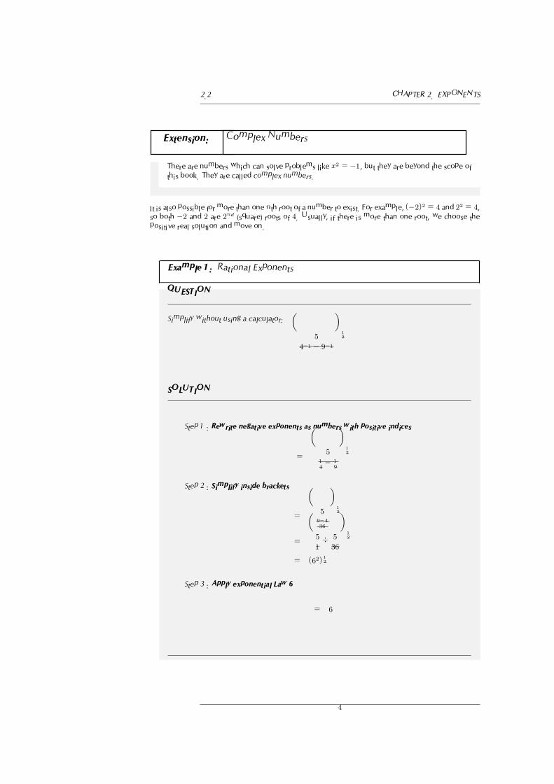
Extension: Complex Numbers
There are numbers which can solve problems like x2 = −1, but they are beyond the scope of
this book. They are called complex numbers.
It is also possible for more than one nth root of a number to exist. For example, (−2)2 = 4 and 22 = 4,so both −2 and 2 are 2nd (square) roots of 4. Usually, if there is more than one root, we choose the
positive real solution and move on.
Example 1: Rational Exponents
QUESTION
Simplify without using a calculator:
�
5
4−1 − 9−1
� 1
2
SOLUTION
Step 1 : Rewrite negative exponents as numbers with positive indices
=
�
514− 1
9
� 1
2
Step 2 : Simplify inside brackets
=
�
59−436
� 1
2
=
�
5
1÷ 5
36
� 1
2
= (62)1
2
Step 3 : Apply exponential Law 6
= 6
4

CHAPTER 2. EXPONENTS 2.2
Example 2: More rational Exponents
QUESTION
Simplify:
(16x4)3
4
SOLUTION
Step 1 : Convert the number coefficient to a product of it’s prime factors
= (24x4)3
4
Step 2 : Apply exponential laws
= 24×3
4 .x4× 3
4
= 23.x3
= 8x3
See video: VMebb at www.everythingmaths.co.za
Exercise 2 - 1
Use all the laws to:
1. Simplify:
(a) (x0) + 5x0 − (0,25)−0,5 + 82
3
(b) s1
2 ÷ s1
3
(c) (64m6)2
3
(d)12m
7
9
8m− 11
9
2. Re-write the following expression as a power of x:
x
�
x
�
x
�
x√x
5

2.3 CHAPTER 2. EXPONENTS
More practice video solutions or help at www.everythingmaths.co.za
(1.) 016e (2.) 016f
2.3 Exponentials in the Real World EMBE
In Grade 10 Finance, you used exponentials to calculate different types of interest, for example on a
savings account or on a loan and compound growth.
Example 3: Exponentials in the Real world
QUESTION
A type of bacteria has a very high exponential growth rate at 80% every hour. If there are 10bacteria, determine how many there will be in five hours, in one day and in one week?
SOLUTION
Step 1 : Population = Initial population × (1 + growth percentage)time period in hours
Therefore, in this case:
Population = 10(1,8)n, where n = number of hours
Step 2 : In 5 hours
Population = 10(1,8)5 = 189
Step 3 : In 1 day = 24 hours
Population = 10(1,8)24 = 13 382 588
Step 4 : in 1 week = 168 hours
Population = 10(1,8)168 = 7,687 × 1043Note this answer is given in scientific notation as it is a very big number.
6

CHAPTER 2. EXPONENTS 2.3
Example 4: More Exponentials in the Real world
QUESTION
A species of extremely rare, deep water fish has an very long lifespan and rarely has children.
If there are a total 821 of this type of fish and their growth rate is 2% each month, how many
will there be in half of a year? What will the population be in ten years and in one hundred
years?
SOLUTION
Step 1 : Population = Initial population × (1+ growth percentage)time period in months
Therefore, in this case:
Population = 821(1,02)n, where n = number of months
Step 2 : In half a year = 6 months
Population = 821(1,02)6 = 925
Step 3 : In 10 years = 120 months
Population = 821(1,02)120 = 8 838
Step 4 : in 100 years = 1 200 months
Population = 821(1,02)1 200 = 1,716× 1013Note this answer is also given in scientific notation as it is a very big number.
Chapter 2 End of Chapter Exercises
1. Simplify as far as possible:
(a) 8−2
3
(b)√16 + 8−
2
3
2. Simplify:
a. (x3)4
3
b. (s2)1
2
c. (m5)5
3
d. (−m2)4
3
e. −(m2)4
3
f. (3y4
3 )4
3. Simplify as much as you can:
3a−2b15c−5
(a−4b3c)−5
2
7

2.3 CHAPTER 2. EXPONENTS
4. Simplify as much as you can:�
9a6b4�
1
2
5. Simplify as much as you can:�
a3
2 b3
4
�16
6. Simplify:
x3√x
7. Simplify:3√x4b5
8. Re-write the following expression as a power of x:
x
�
x
�
x�
x√x
3√x
More practice video solutions or help at www.everythingmaths.co.za
(1.) 016g (2.) 016h (3.) 016i (4.) 016j (5.) 016k (6.) 016m
(7.) 016n (8.) 016p
8

Surds 3
3.1 Introduction EMBF
In the previous chapter on exponents, we saw that rational exponents are directly related to surds.
We will discuss surds and the laws that govern them further here. While working with surds, always
remember that they are directly related to exponents and that you can use your knowledge of one to
help with understanding the other.
See introductory video: VMebn at www.everythingmaths.co.za
3.2 Surd Calculations EMBG
There are several laws that make working with surds (or roots) easier. We will list them all and then
explain where each rule comes from in detail.
n√a
n√b =
n√ab (3.1)
n
�
a
b=
n√a
n√b
(3.2)
n√am = a
mn (3.3)
Surd Law 1: n√a
n√b = n
√ab EMBH
It is often useful to look at a surd in exponential notation as it allows us to use the exponential laws we
learnt in Grade 10. In exponential notation, n√a = a
1
n andn√b = b
1
n . Then,
n√a
n√b = a
1
n b1
n (3.4)
= (ab)1
n
=n√ab
Some examples using this law:
1. 3√16× 3
√4
= 3√64
= 4
2.√2×
√32
=√64
= 8
9

3.2 CHAPTER 3. SURDS
3.√a2b3 ×
√b5c4
=√a2b8c4
= ab4c2
Surd Law 2: n�
ab=
n√a
n√b
EMBI
If we look at n�
abin exponential notation and apply the exponential laws then,
n
�
a
b=
�a
b
� 1
n(3.5)
=a
1
n
b1
n
=n√a
n√b
Some examples using this law:
1.√12÷
√3
=√4
= 2
2. 3√24÷ 3
√3
= 3√8
= 2
3.√a2b13 ÷
√b5
=√a2b8
= ab4
Surd Law 3: n√am = a
mn EMBJ
If we look at n√am in exponential notation and apply the exponential laws then,
n√am = (am)
1
n (3.6)
= amn
For example,
6√23 = 2
3
6
= 21
2
=√2
10

CHAPTER 3. SURDS 3.2
Like and Unlike Surds EMBK
Two surds m√a and
n√b are called like surds if m = n, otherwise they are called unlike surds. For
example√2 and
√3 are like surds, however
√2 and 3
√2 are unlike surds. An important thing to
realise about the surd laws we have just learnt is that the surds in the laws are all like surds.
If we wish to use the surd laws on unlike surds, then we must first convert them into like surds. In
order to do this we use the formula
n√am =
bn√abm (3.7)
to rewrite the unlike surds so that bn is the same for all the surds.
Example 1: Like and Unlike Surds
QUESTION
Simplify to like surds as far as possible, showing all steps: 3√3× 5
√5
SOLUTION
Step 1 : Find the common root
=15√35 × 15
√53
Step 2 : Use surd Law 1
=15√35.53
= 15√243× 125
=15√30375
11

3.2 CHAPTER 3. SURDS
Simplest Surd Form EMBL
In most cases, when working with surds, answers are given in simplest surd form. For example,
√50 =
√25× 2
=√25×
√2
= 5√2
5√2 is the simplest surd form of
√50.
Example 2: Simplest surd form
QUESTION
Rewrite√18 in the simplest surd form:
SOLUTION
Step 1 : Convert the number 18 into a product of it’s prime factors
√18 =
√2× 9
=√2×
√32
Step 2 : Square root all squared numbers:
= 3√2
Example 3: Simplest surd form
12

CHAPTER 3. SURDS 3.2
QUESTION
Simplify:√147 +
√108
SOLUTION
Step 1 : Simplify each square root by converting each number to a product of it’s prime
factors
√147 +
√108 =
√49× 3 +
√36× 3
=�
72 × 3 +�
62 × 3
Step 2 : Square root all squared numbers
= 7√3 + 6
√3
Step 3 : The exact same surds can be treated as ”like terms” and may be added
= 13√3
See video: VMecu at www.everythingmaths.co.za
Rationalising Denominators EMBM
It is useful to work with fractions, which have rational denominators instead of surd denominators. It is
possible to rewrite any fraction, which has a surd in the denominator as a fraction which has a rational
denominator. We will now see how this can be achieved.
Any expression of the form√a+
√b (where a and b are rational) can be changed into a rational number
by multiplying by√a−
√b (similarly
√a−
√b can be rationalised by multiplying by
√a+
√b). This
is because
(√a+
√b)(
√a−
√b) = a− b (3.8)
which is rational (since a and b are rational).
If we have a fraction which has a denominator which looks like√a+
√b, then we can simply multiply
the fraction by√a−
√b
√a−
√bto achieve a rational denominator. (Remember that
√a−
√b
√a−
√b= 1)
c√a+
√b
=
√a−
√b
√a−
√b× c
√a+
√b
(3.9)
=c√a− c
√b
a− b
13

3.2 CHAPTER 3. SURDS
or similarly
c√a−
√b
=
√a+
√b
√a+
√b× c
√a−
√b
(3.10)
=c√a+ c
√b
a− b
Example 4: Rationalising the Denominator
QUESTION
Rationalise the denominator of: 5x−16√x
SOLUTION
Step 1 : Rationalise the denominator
To get rid of√x in the denominator, you can multiply it out by another
√x. This
rationalises the surd in the denominator. Note that√x√x= 1, thus the equation
becomes rationalised by multiplying by 1 (although its’ value stays the same).
5x− 16√x
×√x√x
Step 2 : Multiply out the numerators and denominators
The surd is expressed in the numerator which is the preferred way to write ex-
pressions. (That’s why denominators get rationalised.)
5x√x− 16√x
x
=(√x)(5x− 16)
x
Example 5: Rationalising the Denominator
QUESTION
Rationalise the following: 5x−16√y−10
SOLUTION
Step 1 : Rationalise the denominator
14

CHAPTER 3. SURDS 3.2
5x− 16√y − 10 ×
√y + 10
√y + 10
Step 2 : Multiply out the numerators and denominators
5x√y − 16√y + 50x− 160
y − 100
All the terms in the numerator are different and cannot be simplified and the
denominator does not have any surds in it anymore.
Example 6: Rationalise the denominator
QUESTION
Simplify the following: y−25√y+5
SOLUTION
Step 1 : Rationalise the denominator
y − 25√y + 5
×√y − 5
√y − 5
Step 2 : Multiply out the numerators and denominators
y√y − 25√y − 5y + 125
y − 25 =
√y(y − 25)− 5(y − 25)
(y − 25)
=(y − 25)(√y − 25)
(y − 25)=
√y − 25
See video: VMeea at www.everythingmaths.co.za
Chapter 3 End of Chapter Exercises
15

3.2 CHAPTER 3. SURDS
1. Expand:
(√x−
√2)(
√x+
√2)
2. Rationalise the denominator:10√x− 1
x
3. Write as a single fraction:3
2√x+
√x
4. Write in simplest surd form:
(a)√72
(b)√45 +
√80
(c)
√48√12
(d)
√18÷
√72√
8
(e)4
(√8÷
√2)
(f)16
(√20÷
√12)
5. Expand and simplify:
(2 +√2)2
6. Expand and simplify:
(2 +√2)(1 +
√8)
7. Expand and simplify:
(1 +√3)(1 +
√8 +
√3)
8. Simplify, without use of a calculator:√5(√45 + 2
√80)
9. Simplify: √98x6 +
√128x6
10. Write the following with a rational denominator:√5 + 2√5
11. Simplify, without use of a calculator:√98−
√8√
50
12. Rationalise the denominator:y − 4√y − 2
13. Rationalise the denominator:2x− 20
√y −
√10
14. Evaluate without using a calculator:
�
2−√7
2
�
12
�
2 +
√7
2
�
12
15. Prove (without the use of a calculator) that:�
8
3+ 5
�
5
3−
�
1
6=10
√15 + 3
√6
6
16

CHAPTER 3. SURDS 3.2
16. The use of a calculator is not permissible in this question. Simplify completely by
showing all your steps: 3−12
�√12 + 3
�
(3√3)
�
17. Fill in the blank surd-form number on the right hand side of the equation which will
make the following a true statement: −3√6×−2
√24 = −
√18× . . . . . .
More practice video solutions or help at www.everythingmaths.co.za
(1.) 016q (2.) 016r (3.) 016s (4.) 016t (5.) 016u (6.) 016v
(7.) 016w (8.) 016x (9.) 016y (10.) 016z (11.) 0170 (12.) 0171
(13.) 0172 (14.) 0173 (15.) 0174 (16.) 0175 (17.) 0176
17
Error Margins 4
4.1 Introduction EMBN
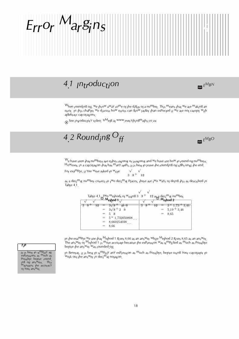
When rounding off, we throw away some of the digits of a number. This means that we are making an
error. In this chapter we discuss how errors can grow larger than expected if we are not careful with
algebraic calculations.
See introductory video: VMefg at www.everythingmaths.co.za
4.2 Rounding Off EMBO
We have seen that numbers are either rational or irrational and we have see how to round off numbers.
However, in a calculation that has many steps, it is best to leave the rounding off right until the end.
For example, if you were asked to write
3√3 +
√12
as a decimal number correct to two decimal places, there are two ways of doing this as described in
Table 4.1.
Table 4.1: Two methods of writing 3√3 +
√12 as a decimal number.
� Method 1 � Method 2
3√3 +
√12 = 3
√3 +
√4 . 3 3
√3 +
√12 = 3× 1,73 + 3,46
= 3√3 + 2
√3 = 5,19 + 3,46
= 5√3 = 8,65
= 5× 1,732050808 . . .= 8,660254038 . . .= 8,66
In the example we see that Method 1 gives 8,66 as an answer while Method 2 gives 8,65 as an answer.The answer of Method 1 is more accurate because the expression was simplified as much as possible
before the answer was rounded-off.
In general, it is best to simplify any expression as much as possible, before using your calculator to
work out the answer in decimal notation.
Tip
It is best to simplify allexpressions as much aspossible before round-ing off answers. Thismaintains the accuracyof your answer.
18

CHAPTER 4. ERROR MARGINS 4.2
Example 1: Simplification and Accuracy
QUESTION
Calculate 3√54 + 3
√16. Write the answer to three decimal places.
SOLUTION
Step 1 : Simplify the expression
3√54 +
3√16 =
3√27 . 2 +
3√8 . 2
=3√27 .
3√2 +
3√8 .
3√2
= 33√2 + 2
3√2
= 53√2
Step 2 : Convert any irrational numbers to decimal numbers
53√2 = 6,299605249 . . .
Step 3 : Write the final answer to the required number of decimal places.
6,299605249 . . . = 6,300 (to three decimal places)
∴3√54 + 3
√16 = 6,300 (to three decimal places).
Example 2: Simplification and Accuracy 2
QUESTION
Calculate√x+ 1+ 1
3
�
(2x+ 2)− (x+ 1) if x = 3,6. Write the answer to two decimal places.
SOLUTION
Step 1 : Simplify the expression
19

4.2 CHAPTER 4. ERROR MARGINS
√x+ 1 +
1
3
�
(2x+ 2)− (x+ 1) =√x+ 1 +
1
3
√2x+ 2− x− 1
=√x+ 1 +
1
3
√x+ 1
=4
3
√x+ 1
Step 2 : Substitute the value of x into the simplified expression
4
3
√x+ 1 =
4
3
�
3,6 + 1
=4
3
�
4,6
= 2,859681412 . . .
Step 3 : Write the final answer to the required number of decimal places.
2,859681412 . . . = 2,86 (To two decimal places)
∴√x+ 1 + 1
3
�
(2x+ 2)− (x+ 1) = 2,86 (to two decimal places) if x = 3,6.
Extension: Significant Figures
In a number, each non-zero digit is a significant figure. Zeroes are only counted if they are
between two non-zero digits or are at the end of the decimal part. For example, the number
2000 has one significant figure (the 2), but 2000,0 has five significant figures. Estimating a
number works by removing significant figures from your number (starting from the right) until
you have the desired number of significant figures, rounding as you go. For example 6,827has four significant figures, but if you wish to write it to three significant figures it would mean
removing the 7 and rounding up, so it would be 6,83. It is important to know when to estimate
a number and when not to. It is usually good practise to only estimate numbers when it is
absolutely necessary, and to instead use symbols to represent certain irrational numbers (such
as π); approximating them only at the very end of a calculation. If it is necessary to approximate
a number in the middle of a calculation, then it is often good enough to approximate to a few
decimal places.
Chapter 4 End of Chapter Exercises
1. Calculate:
(a)√16
√72 to three decimal places
(b)√25 +
√2 to one decimal place
(c)√48
√3 to two decimal places
(d)√64 +
√18
√12 to two decimal places
20

CHAPTER 4. ERROR MARGINS 4.2
(e)√4 +
√20
√18 to six decimal places
(f)√3 +
√5√6 to one decimal place
2. Calculate:
(a)√x2 , if x = 3,3. Write the answer to four decimal places.
(b)√4 + x , if x = 1,423. Write the answer to two decimal places.
(c)√x+ 3 +
√x , if x = 5,7. Write the answer to eight decimal places.
(d)√2x5 + 1
2
√x+ 1 , if x = 4,91. Write the answer to five decimal places.
(e)�
3x1 + (4x+ 3)√x+ 5 , if x = 3,6. Write the answer to six decimal places.
(f)�
2x+ 5(x1) + (5x+ 2) + 14
√4 + x, if x = 1,09. Write the answer to one
decimal place
More practice video solutions or help at www.everythingmaths.co.za
(1.) 02sf (2.) 02sg
21

Quadratic Sequences 5
5.1 Introduction EMBP
In Grade 10 you learned about arithmetic sequences, where the difference between consecutive terms
is constant. In this chapter we learn about quadratic sequences, where the difference between consec-
utive terms is not constant, but follows its own pattern.
See introductory video: VMeka at www.everythingmaths.co.za
5.2 What is a Quadratic Sequence? EMBQ
DEFINITION: Quadratic Sequence
A quadratic sequence is a sequence of numbers in which the second difference be-
tween each consecutive term is constant. This called a common second difference.
For example,
1; 2; 4; 7; 11; . . . (5.1)
is a quadratic sequence. Let us see why.
The first difference is calculated by finding the difference between consecutive terms:
1 2 4 7 11
+1 +2 +3 +4
We then work out the second differences, which are simply obtained by taking the difference between
the consecutive differences {1; 2; 3; 4; . . .} obtained above:
1 2 3 4
+1 +1 +1
We then see that the second differences are equal to 1. Thus, Equation (5.1) is a quadratic sequence.
Note that the differences between consecutive terms (that is, the first differences) of a quadratic se-
quence form a sequence where there is a constant difference between consecutive terms. In the above
example, the sequence of {1; 2; 3; 4; . . .}, which is formed by taking the differences between consec-utive terms of Equation (5.1), has a linear formula of the kind ax+ b.
Exercise 5 - 1
The following are examples of quadratic sequences:
22

CHAPTER 5. QUADRATIC SEQUENCES 5.2
1. 3; 6; 10; 15; 21; . . .
2. 4; 9; 16; 25; 36; . . .
3. 7; 17; 31; 49; 71; . . .
4. 2; 10; 26; 50; 82; . . .
5. 31; 30; 27; 22; 15; . . .
Calculate the common second difference for each of the above examples.
More practice video solutions or help at www.everythingmaths.co.za
(1.-5.) 01zm
General Case
If the sequence is quadratic, the nth term should be Tn = an2 + bn+ c
TERMS a+ b+ c 4a+ 2b+ c 9a+ 3b+ c 16a+ 4b+ c
1st difference 3a+ b 5a+ b 7a+ b
2nd difference 2a 2a
In each case, the second difference is 2a. This fact can be used to find a, then b then c.
Example 1: Quadratic sequence
QUESTION
Write down the next two terms and find a formula for the nth term of the sequence 5; 12; 23; 38; . . .
SOLUTION
Step 1 : Find the first differences between the terms
5 12 23 38
+7 +11 +15
i.e. 7; 11; 15.
23

5.2 CHAPTER 5. QUADRATIC SEQUENCES
Step 2 : Find the second differences between the terms
7 11 15
+4 +4
So the second difference is 4.Continuing the sequence, the differences between each term will be:
...15 19 23...
+4 +4
Step 3 : Finding the next two terms
The next two terms in the sequence will be:
...38 57 80...
+19 +23
So the sequence will be: 5; 12; 23; 38; 57; 80.
Step 4 : Determine values for a, b and c
2a = 4
which gives a = 2
And 3a+ b = 7
∴ 3(2) + b = 7
b = 7− 6b = 1
And a+ b+ c = 5
∴ (2) + (1) + c = 5
c = 5− 3c = 2
Step 5 : Find the rule by substitution
Tn = ax2 + bx+ c
∴ Tn = 2n2 + n+ 2
Example 2: Quadratic Sequence
24

CHAPTER 5. QUADRATIC SEQUENCES 5.2
QUESTION
The following sequence is quadratic: 8; 22; 42; 68; . . . Find the rule.
SOLUTION
Step 1 : Assume that the rule is an2 + bn+ c
TERMS 8 22 42 68
1st difference +14 +20 +26
2nd difference +6 +6
Step 2 : Determine values for a, b and c
2a = 6
which gives a = 3
And 3a+ b = 14
∴ 9 + b = 14
b = 5
And a+ b+ c = 8
∴ 3 + 5 + c = 8
c = 0
Step 3 : Find the rule by substitution
Tn = ax2 + bx+ c
∴ Tn = 3n2 + 5n
Step 4 : Check answer
For
n = 1, T1 = 3(1)2 + 5(1) = 8
n = 2, T2 = 3(2)2 + 5(2) = 22
n = 3, T3 = 3(3)2 + 5(3) = 42
Extension: Derivation of the nth-term of a Quadratic Sequence
Let the nth-term for a quadratic sequence be given by
Tn = an2 + bn+ c (5.2)
25

5.2 CHAPTER 5. QUADRATIC SEQUENCES
where a, b and c are some constants to be determined.
Tn = an2 + bn+ c
T1 = a(1)2 + b(1) + c
= a+ b+ c (5.3)
T2 = a(2)2 + b(2) + c
= 4a+ 2b+ c (5.4)
T3 = a(3)2 + b(3) + c
= 9a+ 3b+ c (5.5)
The first difference (d) is obtained from
Let d ≡ T2 − T1
∴ d = 3a+ b
⇒ b = d− 3a (5.6)
The common second difference (D) is obtained from
D = (T3 − T2)− (T2 − T1)
= (5a+ b)− (3a+ b)
= 2a
⇒ a =D
2(5.7)
Therefore, from (5.6),
b = d− 3
2. D (5.8)
From (5.3),
c = T1 − (a+ b) = T1 −D
2− d+
3
2. D
∴ c = T1 +D − d (5.9)
Finally, the general equation for the nth-term of a quadratic sequence is given by
Tn =D
2. n2 + (d− 3
2D) . n+ (T1 − d+D) (5.10)
Example 3: Using a set of equations
QUESTION
Study the following pattern: 1; 7; 19; 37; 61; . . .
1. What is the next number in the sequence?
2. Use variables to write an algebraic statement to generalise the pattern.
3. What will the 100th term of the sequence be?
26

CHAPTER 5. QUADRATIC SEQUENCES 5.2
SOLUTION
Step 1 : The next number in the sequence
The numbers go up in multiples of 61 + 6(1) = 7, then 7 + 6(2) = 1919 + 6(3) = 37, then 37 + 6(4) = 61Therefore 61 + 6(5) = 91The next number in the sequence is 91.
Step 2 : Generalising the pattern
TERMS 1 7 19 37 61
1st difference +6 +12 +18 +24
2nd difference +6 +6 +6
The pattern will yield a quadratic equation since the second difference is
constant
Therefore Tn = an2 + bn+ cFor the first term: n = 1, then T1 = 1For the second term: n = 2, then T2 = 7For the third term: n = 3, then T3 = 19etc.
Step 3 : Setting up sets of equations
a+ b+ c = 1 ...eqn(1)
4a+ 2b+ c = 7 ...eqn(2)
9a+ 3b+ c = 19 ...eqn(3)
Step 4 : Solve the sets of equations
eqn(2)− eqn(1) : 3a+ b = 6 ...eqn(4)
eqn(3)− eqn(2) : 5a+ b = 12 ...eqn(5)
eqn(5)− eqn(4) : 2a = 6
∴ a = 3, b = −3 and c = 1
Step 5 : Final answer
The general formula for the pattern is Tn = 3n2 − 3n+ 1
Step 6 : Term 100
Substitute n with 100:3(100)2 − 3(100) + 1 = 29 701The value for term 100 is 29 701.
27

5.2 CHAPTER 5. QUADRATIC SEQUENCES
Extension: Plotting a graph of terms of a quadratic sequence
Plotting Tn vs. n for a quadratic sequence yields a parabolic graph.
Given the quadratic sequence,
3; 6; 10; 15; 21; . . .
If we plot each of the terms vs. the corresponding index, we obtain a graph of a parabola.
�
�
�
�
�
�
�
�
�
�
Term
:Tn
y-intercept: T1
1 2 3 4 5 6 7 8 9 10
Index: n
a1
a2
a3
a4
a5
a6
a7
a8
a9
a10
Chapter 5 End of Chapter Exercises
1. Find the first five terms of the quadratic sequence defined by:
an = n2 + 2n+ 1
2. Determine which of the following sequences is a quadratic sequence by calculating
the common second difference:
(a) 6; 9; 14; 21; 30; . . .
(b) 1; 7; 17; 31; 49; . . .
(c) 8; 17; 32; 53; 80; . . .
(d) 9; 26; 51; 84; 125; . . .
(e) 2; 20; 50; 92; 146; . . .
(f) 5; 19; 41; 71; 109; . . .
(g) 2; 6; 10; 14; 18; . . .
28

CHAPTER 5. QUADRATIC SEQUENCES 5.2
(h) 3; 9; 15; 21; 27; . . .
(i) 10; 24; 44; 70; 102; . . .
(j) 1; 2,5; 5; 8,5; 13; . . .
(k) 2,5; 6; 10,5; 16; 22,5; . . .
(l) 0,5; 9; 20,5; 35; 52,5; . . .
3. Given Tn = 2n2, find for which value of n, Tn = 242
4. Given Tn = (n− 4)2, find for which value of n, Tn = 36
5. Given Tn = n2 + 4, find for which value of n, Tn = 85
6. Given Tn = 3n2, find T11
7. Given Tn = 7n2 + 4n, find T9
8. Given Tn = 4n2 + 3n− 1, find T5
9. Given Tn = 1,5n2, find T10
10. For each of the quadratic sequences, find the common second difference, the formula
for the general term and then use the formula to find a100.
(a) 4; 7; 12; 19; 28; . . .
(b) 2; 8; 18; 32; 50; . . .
(c) 7; 13; 23; 37; 55; . . .
(d) 5; 14; 29; 50; 77; . . .
(e) 7; 22; 47; 82; 127; . . .
(f) 3; 10; 21; 36; 55; . . .
(g) 3; 7; 13; 21; 31; . . .
(h) 3; 9; 17; 27; 39; . . .
More practice video solutions or help at www.everythingmaths.co.za
(1.) 0177 (2.) 0178 (3.) 0179 (4.) 017a (5.) 017b (6.) 017c
(7.) 017d (8.) 017e (9.) 017f (10.) 017g
29

Finance 6
6.1 Introduction EMBR
In Grade 10, the concepts of simple and compound interest were introduced. Here we will extend
those concepts, so it is a good idea to revise what you’ve learnt. After you have mastered the techniques
in this chapter, you will understand depreciation and will learn how to determine which bank is
offering the best interest rate.
See introductory video: VMemn at www.everythingmaths.co.za
6.2 Depreciation EMBS
It is said that when you drive a new car out of the dealership, it loses 20% of its value, because it is
now “second-hand”. And from there on the value keeps falling, or depreciating. Second hand cars are
cheaper than new cars, and the older the car, usually the cheaper it is. If you buy a second-hand (or
should we say pre-owned!) car from a dealership, they will base the price on something called book
value.
The book value of the car is the value of the car taking into account the loss in value due to wear, age
and use. We call this loss in value depreciation, and in this section we will look at two ways of how
this is calculated. Just like interest rates, the two methods of calculating depreciation are simple and
compound methods.
The terminology used for simple depreciation is straight-line depreciation and for compound depre-
ciation is reducing-balance depreciation. In the straight-line method the value of the asset is reduced
by the same constant amount each year. In compound depreciation or reducing-balance the value of
the asset is reduced by the same percentage each year. This means that the value of an asset does not
decrease by a constant amount each year, but the decrease is most in the first year, then by a smaller
amount in the second year and by an even smaller amount in the third year, and so on.
Extension: Depreciation
You may be wondering why we need to calculate depreciation. Determining the value of assets
(as in the example of the second hand cars) is one reason, but there is also a more financial
reason for calculating depreciation — tax! Companies can take depreciation into account as
an expense, and thereby reduce their taxable income. A lower taxable income means that the
company will pay less income tax to the Revenue Service.
30

CHAPTER 6. FINANCE 6.3
6.3 Simple Decay or Straight-linedepreciation
EMBT
Let us return to the second-hand cars. One way of calculating a depreciation amount would be to
assume that the car has a limited useful life. Simple depreciation assumes that the value of the car
decreases by an equal amount each year. For example, let us say the limited useful life of a car is 5
years, and the cost of the car today is R60 000. What we are saying is that after 5 years you will have
to buy a new car, which means that the old one will be valueless at that point in time. Therefore, the
amount of depreciation is calculated:
R60 000
5 years= R12 000 per year.
The value of the car is then:
End of Year 1 R60 000− 1× (R12 000) = R48 000End of Year 2 R60 000− 2× (R12 000) = R36 000End of Year 3 R60 000− 3× (R12 000) = R24 000End of Year 4 R60 000− 4× (R12 000) = R12 000End of Year 5 R60 000− 5× (R12 000) = R0
This looks similar to the formula for simple interest:
Total Interest after n years = n× (P × i)
where i is the annual percentage interest rate and P is the principal amount.
If we replace the word interest with the word depreciation and the word principal with the words
initial value we can use the same formula:
Total depreciation after n years = n× (P × i)
Then the book value of the asset after n years is:
Initial Value – Total depreciation after n years = P − n× (P × i)
A = P (1− n× i)
For example, the book value of the car after two years can be simply calculated as follows:
Book Value after 2 years = P (1− n× i)
= R60 000(1− 2× 20%)= R60 000(1− 0,4)= R60 000(0,6)
= R36 000
as expected.
Note that the difference between the simple interest calculations and the simple decay calculations is
that while the interest adds value to the principal amount, the depreciation amount reduces value!
31

6.3 CHAPTER 6. FINANCE
Example 1: Simple Decay method
QUESTION
A car is worth R240 000 now. If it depreciates at a rate of 15% p.a. on a straight-line depreci-
ation, what is it worth in 5 years’ time?
SOLUTION
Step 1 : Determine what has been provided and what is required
P = R240 000
i = 0,15
n = 5
A is required
Step 2 : Determine how to approach the problem
A = P (1− i× n)
A = 240 000(1− (0,15× 5))
Step 3 : Solve the problem
A = 240 000(1− 0,75)= 240 000× 0,25= 60 000
Step 4 : Write the final answer
In 5 years’ time the car is worth R60 000
Example 2: Simple Decay
QUESTION
A small business buys a photocopier for R12 000. For the tax return the owner depreciates thisasset over 3 years using a straight-line depreciation method. What amount will he fill in on
32

CHAPTER 6. FINANCE 6.3
his tax form after 1 year, after 2 years and then after 3 years?
SOLUTION
Step 1 : Understanding the question
The owner of the business wants the photocopier to depreciate to R0 after 3
years. Thus, the value of the photocopier will go down by 12 000 ÷ 3 = R4 000per year.
Step 2 : Value of the photocopier after 1 year
12 000− 4 000 = R8 000
Step 3 : Value of the machine after 2 years
8 000− 4 000 = R4 000
Step 4 : Write the final answer
4 000− 4 000 = 0After 3 years the photocopier is worth nothing
Extension: Salvage Value
Looking at the same example of our car with an initial value of R60 000, what if we supposethat we think we would be able to sell the car at the end of the 5 year period for R10 000? We
call this amount the “Salvage Value”.
We are still assuming simple depreciation over a useful life of 5 years, but now instead
of depreciating the full value of the asset, we will take into account the salvage value, and
will only apply the depreciation to the value of the asset that we expect not to recoup, i.e.
R60 000−R10 000 =R50 000.The annual depreciation amount is then calculated as (R60 000−R10 000)/5 =R10000In general, the formula for simple (straight line) depreciation:
Annual Depreciation =Initial Value – Salvage Value
Useful Life
Exercise 6 - 1
1. A business buys a truck for R560 000. Over a period of 10 years the value of the truck depreciatesto R0 (using the straight-line method). What is the value of the truck after 8 years?
2. Shrek wants to buy his grandpa’s donkey for R800. His grandpa is quite pleased with the offer,
seeing that it only depreciated at a rate of 3% per year using the straight-line method. Grandpa
bought the donkey 5 years ago. What did grandpa pay for the donkey then?
3. Seven years ago, Rocco’s drum kit cost him R12 500. It has now been valued at R2 300. What
rate of simple depreciation does this represent?
4. Fiona buys a DStv satellite dish for R3 000. Due to weathering, its value depreciates simply at
15% per annum. After how long will the satellite dish be worth nothing?
33

6.4 CHAPTER 6. FINANCE
More practice video solutions or help at www.everythingmaths.co.za
(1.) 017h (2.) 017i (3.) 017j (4.) 017k
6.4 Compound Decay orReducing-balance depreciation
EMBU
The second method of calculating depreciation is to assume that the value of the asset decreases at a
certain annual rate, but that the initial value of the asset this year, is the book value of the asset at the
end of last year.
For example, if our second hand car has a limited useful life of 5 years and it has an initial value of
R60 000, then the interest rate of depreciation is 20% (100%/5 years). After 1 year, the car is worth:
Book Value after first year = P (1− n× i)
= R60 000(1− 1× 20%)= R60 000(1− 0,2)= R60 000(0,8)
= R48 000
At the beginning of the second year, the car is now worth R48 000, so after two years, the car is worth:
Book Value after second year = P (1− n× i)
= R48 000(1− 1× 20%)= R48 000(1− 0,2)= R48 000(0,8)
= R38 400
We can tabulate these values.
End of first year R60 000(1− 1× 20%) =R60 000(1− 1× 20%)1 = R48 000,00End of second year R48 000(1− 1× 20%) =R60 000(1− 1× 20%)2 = R38 400,00End of third year R38 400(1− 1× 20%) =R60 000(1− 1× 20%)3 = R30 720,00End of fourth year R30 720(1− 1× 20%) =R60 000(1− 1× 20%)4 = R24 576,00End of fifth year R24 576(1− 1× 20%) =R60 000(1− 1× 20%)5 = R19 608,80
We can now write a general formula for the book value of an asset if the depreciation is compounded.
Initial Value – Total depreciation after n years = P (1− i)n (6.1)
For example, the book value of the car after two years can be simply calculated as follows:
Book Value after 2 years: A = P (1− i)n
= R60 000(1− 20%)2
= R60 000(1− 0,2)2
= R60 000(0,8)2
= R38 400
as expected.
Note that the difference between the compound interest calculations and the compound depreciation
calculations is that while the interest adds value to the principal amount, the depreciation amount
reduces value!
34

CHAPTER 6. FINANCE 6.4
Example 3: Compound Depreciation
QUESTION
The flamingo population of the Berg river mouth is depreciating on a reducing balance at a
rate of 12% p.a. If there are now 3 200 flamingos in the wetlands of the Berg river mouth, howmany will there be in 5 years’ time? Answer to three significant figures.
SOLUTION
Step 1 : Determine what has been provided and what is required
P = 3 200
i = 0,12
n = 5
A is required
Step 2 : Determine how to approach the problem
A = P (1− i)n
A = 3 200(1− 0,12)5
Step 3 : Solve the problem
A = 3 200(0,88)5
= 1688,742134
Step 4 : Write the final answer
There would be approximately 1 690 flamingos in 5 years’ time.
Example 4: Compound Depreciation
QUESTION
Farmer Brown buys a tractor for R250 000 which depreciates by 20% per year using the com-
pound depreciation method. What is the depreciated value of the tractor after 5 years?
35

6.4 CHAPTER 6. FINANCE
SOLUTION
Step 1 : Determine what has been provided and what is required
P = R250 000
i = 0,2
n = 5
A is required
Step 2 : Determine how to approach the problem
A = P (1− i)n
A = 250 000(1− 0,2)5
Step 3 : Solve the problem
A = 250 000(0,8)5
= 81 920
Step 4 : Write the final answer
Depreciated value after 5 years is R81 920
Exercise 6 - 2
1. On January 1, 2008 the value of my Kia Sorento is R320 000. Each year after that, the cars valuewill decrease 20% of the previous years value. What is the value of the car on January 1, 2012?
2. The population of Bonduel decreases at a reducing-balance rate of 9,5% per annum as people
migrate to the cities. Calculate the decrease in population over a period of 5 years if the initial
population was 2 178 000.
3. A 20 kg watermelon consists of 98% water. If it is left outside in the sun it loses 3% of its water
each day. How much does it weigh after a month of 31 days?
4. A computer depreciates at x% per annum using the reducing-balance method. Four years ago
the value of the computer was R10 000 and is now worth R4 520. Calculate the value of x correct
to two decimal places.
More practice video solutions or help at www.everythingmaths.co.za
(1.) 017m (2.) 017n (3.) 017p (4.) 017q
36

CHAPTER 6. FINANCE 6.5
6.5 Present and Future Values ofan Investment or Loan
EMBV
Now or Later EMBW
When we studied simple and compound interest we looked at having a sum of money now, and
calculating what it will be worth in the future. Whether the money was borrowed or invested, the
calculations examined what the total money would be at some future date. We call these future
values.
It is also possible, however, to look at a sum of money in the future, and work out what it is worth
now. This is called a present value.
For example, if R1 000 is deposited into a bank account now, the future value is what that amount willaccrue to by some specified future date. However, if R1 000 is needed at some future time, then the
present value can be found by working backwards — in other words, how much must be invested to
ensure the money grows to R1 000 at that future date?
The equation we have been using so far in compound interest, which relates the open balance (P ), theclosing balance (A), the interest rate (i as a rate per annum) and the term (n in years) is:
A = P . (1 + i)n (6.2)
Using simple algebra, we can solve for P instead of A, and come up with:
P = A . (1 + i)−n (6.3)
This can also be written as follows, but the first approach is usually preferred.
P =A
(1 + i)n(6.4)
Now think about what is happening here. In Equation 6.2, we start off with a sum of money and we
let it grow for n years. In Equation 6.3 we have a sum of money which we know in n years time, and
we “unwind” the interest — in other words we take off interest for n years, until we see what it is worth
right now.
We can test this as follows. If I have R1 000 now and I invest it at 10% for 5 years, I will have:
A = P . (1 + i)n
= R1 000(1 + 10%)5
= R1 610,51
at the end. BUT, if I know I have to have R1610,51 in 5 years time, I need to invest:
P = A . (1 + i)−n
= R1 610,51(1 + 10%)−5
= R1 000
We end up with R1 000 which — if you think about it for a moment — is what we started off with. Do
you see that?
Of course we could apply the same techniques to calculate a present value amount under simple
interest rate assumptions — we just need to solve for the opening balance using the equations for
simple interest.
37

6.6 CHAPTER 6. FINANCE
A = P (1 + i× n) (6.5)
Solving for P gives:
P =A
(1 + i× n)(6.6)
Let us say you need to accumulate an amount of R1 210 in 3 years time, and a bank
account pays simple interest of 7%. How much would you need to invest in this bank
account today?
P =A
1 + n . i
=R1 210
1 + 3× 7%= R1 000
Does this look familiar? Look back to the simple interest worked example in Grade 10.
There we started with an amount of R1 000 and looked at what it would grow to in 3 years’
time using simple interest rates. Now we have worked backwards to see what amount we
need as an opening balance in order to achieve the closing balance of R1 210.
In practise, however, present values are usually always calculated assuming compound interest. So
unless you are explicitly asked to calculate a present value (or opening balance) using simple interest
rates, make sure you use the compound interest rate formula!
Exercise 6 - 3
1. After a 20-year period Josh’s lump sum investment matures to an amount of R313 550. How
much did he invest if his money earned interest at a rate of 13,65% p.a. compounded half yearly
for the first 10 years, 8,4% p.a. compounded quarterly for the next five years and 7,2% p.a.
compounded monthly for the remaining period?
2. A loan has to be returned in two equal semi-annual instalments. If the rate of interest is 16% per
annum, compounded semi-annually and each instalment is R1 458, find the sum borrowed.
More practice video solutions or help at www.everythingmaths.co.za
(1.) 017r (2.) 017s
6.6 Finding i EMBX
By this stage in your studies of the mathematics of finance, you have always known what interest rate
to use in the calculations, and how long the investment or loan will last. You have then either taken
a known starting point and calculated a future value, or taken a known future value and calculated a
present value.
But here are other questions you might ask:
1. I want to borrow R2 500 from my neighbour, who said I could pay back R3 000 in 8 months
time. What interest is she charging me?
38
CHAPTER 6. FINANCE 6.6
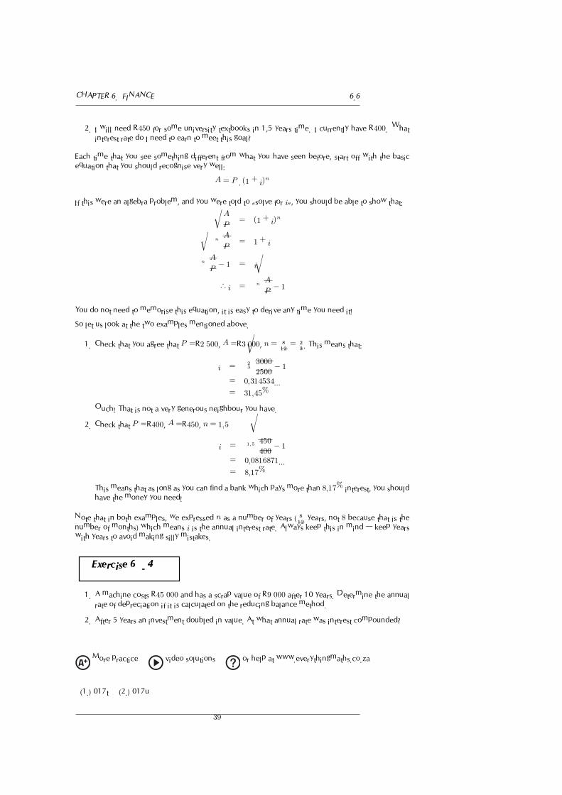
2. I will need R450 for some university textbooks in 1,5 years time. I currently have R400. What
interest rate do I need to earn to meet this goal?
Each time that you see something different from what you have seen before, start off with the basic
equation that you should recognise very well:
A = P . (1 + i)n
If this were an algebra problem, and you were told to “solve for i”, you should be able to show that:
A
P= (1 + i)n
n
�
A
P= 1 + i
n
�
A
P− 1 = i
∴ i =n
�
A
P− 1
You do not need to memorise this equation, it is easy to derive any time you need it!
So let us look at the two examples mentioned above.
1. Check that you agree that P =R2 500, A =R3 000, n = 812= 2
3. This means that:
i =2
3
�
3000
2500− 1
= 0,314534...
= 31,45%
Ouch! That is not a very generous neighbour you have.
2. Check that P =R400, A =R450, n = 1,5
i =1,5
�
450
400− 1
= 0,0816871...
= 8,17%
This means that as long as you can find a bank which pays more than 8,17% interest, you should
have the money you need!
Note that in both examples, we expressed n as a number of years ( 812
years, not 8 because that is thenumber of months) which means i is the annual interest rate. Always keep this in mind — keep years
with years to avoid making silly mistakes.
Exercise 6 - 4
1. A machine costs R45 000 and has a scrap value of R9 000 after 10 years. Determine the annual
rate of depreciation if it is calculated on the reducing balance method.
2. After 5 years an investment doubled in value. At what annual rate was interest compounded?
More practice video solutions or help at www.everythingmaths.co.za
(1.) 017t (2.) 017u
39
6.7 CHAPTER 6. FINANCE
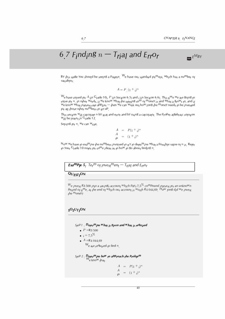
6.7 Finding n — Trial and Error EMBY
By this stage you should be seeing a pattern. We have our standard formula, which has a number of
variables:
A = P . (1 + i)n
We have solved for A (in Grade 10), P (in Section 6.5) and i (in Section 6.6). This time we are going to
solve for n. In other words, if we know what the starting sum of money is and what it grows to, and if
we know what interest rate applies — then we can work out how long the money needs to be invested
for all those other numbers to tie up.
This section will calculate n by trial and error and by using a calculator. The proper algebraic solution
will be learnt in Grade 12.
Solving for n, we can write:
A = P (1 + i)n
A
P= (1 + i)n
Now we have to examine the numbers involved to try to determine what a possible value of n is. Refer
to your Grade 10 notes for some ideas as to how to go about finding n.
Example 5: Term of Investment — Trial and Error
QUESTION
We invest R3 500 into a savings account which pays 7,5% compound interest for an unknown
period of time, at the end of which our account is worth R4 044,69. How long did we invest
the money?
SOLUTION
Step 1 : Determine what is given and what is required
• P =R3 500
• i = 7,5%
• A =R4 044,69
We are required to find n.
Step 2 : Determine how to approach the problem
We know that:
A = P (1 + i)n
A
P= (1 + i)n
40

CHAPTER 6. FINANCE 6.8
Step 3 : Solve the problem
R4 044,69
R3 500= (1 + 7,5%)n
1,156 = (1,075)n
We now use our calculator and try a few values for n.
Possible n 1,075n
1,0 1,0751,5 1,1152,0 1,1562,5 1,198
We see that n is close to 2.
Step 4 : Write final answer
The R3 500 was invested for about 2 years.
Exercise 6 - 5
1. A company buys two types of motor cars: The Acura costs R80 600 and the Brata R101 700,V.A.T. included. The Acura depreciates at a rate, compounded annually, of 15,3% per year and
the Brata at 19,7%, also compounded annually, per year. After how many years will the book
value of the two models be the same?
2. The fuel in the tank of a truck decreases every minute by 5,5% of the amount in the tank at that
point in time. Calculate after how many minutes there will be less than 30 l in the tank if it
originally held 200 l.
More practice video solutions or help at www.everythingmaths.co.za
(1.) 017v (2.) 017w
6.8 Nominal and Effective InterestRates
EMBZ
So far we have discussed annual interest rates, where the interest is quoted as a per annum amount.
Although it has not been explicitly stated, we have assumed that when the interest is quoted as a per
annum amount it means that the interest is paid once a year.
Interest however, may be paid more than just once a year, for example we could receive interest on a
monthly basis, i.e. 12 times per year. So how do we compare a monthly interest rate, say, to an annual
interest rate? This brings us to the concept of the effective annual interest rate.
One way to compare different rates and methods of interest payments would be to compare the closing
balances under the different options, for a given opening balance. Another, more widely used, way is
41

6.8 CHAPTER 6. FINANCE
to calculate and compare the effective annual interest rate on each option. This way, regardless of the
differences in how frequently the interest is paid, we can compare apples-with-apples.
For example, a savings account with an opening balance of R1 000 offers a compound interest rate of
1% per month which is paid at the end of every month. We can calculate the accumulated balance
at the end of the year using the formulae from the previous section. But be careful our interest rate
has been given as a monthly rate, so we need to use the same units (months) for our time period of
measurement.
Tip
Remember, the trick tousing the formulae is todefine the time period,and use the interest raterelevant to the time pe-riod.
So we can calculate the amount that would be accumulated by the end of 1-year as follows:
Closing Balance after 12 months = P × (1 + i)n
= R1 000× (1 + 1%)12
= R1 126,83
Note that because we are using a monthly time period, we have used n = 12 months to calculate the
balance at the end of one year.
The effective annual interest rate is an annual interest rate which represents the equivalent per annum
interest rate assuming compounding.
It is the annual interest rate in our Compound Interest equation that equates to the same accumulated
balance after one year. So we need to solve for the effective annual interest rate so that the accumulated
balance is equal to our calculated amount of R1 126,83.
We use i12 to denote the monthly interest rate. We have introduced this notation here to distinguish
between the annual interest rate, i. Specifically, we need to solve for i in the following equation:
P × (1 + i)1 = P × (1 + i12)12
(1 + i) = (1 + i12)12
divide both sides by P
i = (1 + i12)12 − 1 subtract 1 from both sides
For the example, this means that the effective annual rate for a monthly rate i12 = 1% is:
i = (1 + i12)12 − 1
= (1 + 1%)12 − 1= 0,12683
= 12,683%
If we recalculate the closing balance using this annual rate we get:
Closing Balance after 1 year = P × (1 + i)n
= R1 000× (1 + 12,683%)1
= R1 126,83
which is the same as the answer obtained for 12 months.
Note that this is greater than simply multiplying the monthly rate by (12×1% = 12%) due to the effectsof compounding. The difference is due to interest on interest. We have seen this before, but it is an
important point!
The General Formula EMBAA
So we know how to convert a monthly interest rate into an effective annual interest. Similarly, we can
convert a quarterly or semi-annual interest rate (or an interest rate of any frequency for that matter) into
an effective annual interest rate.
42

CHAPTER 6. FINANCE 6.8
For a quarterly interest rate of say 3% per quarter, the interest will be paid four times per year (every
three months). We can calculate the effective annual interest rate by solving for i:
P (1 + i) = P (1 + i4)4
where i4 is the quarterly interest rate.
So (1 + i) = (1,03)4 , and so i = 12,55%. This is the effective annual interest rate.
In general, for interest paid at a frequency of T times per annum, the follow equation holds:
P (1 + i) = P (1 + iT )T
(6.7)
where iT is the interest rate paid T times per annum.
Decoding the Terminology EMBAB
Market convention however, is not to state the interest rate as say 1% per month, but rather to express
this amount as an annual amount which in this example would be paid monthly. This annual amount
is called the nominal amount.
The market convention is to quote a nominal interest rate of “12% per annum paid monthly” instead
of saying (an effective) 1% per month. We know from a previous example, that a nominal interest
rate of 12% per annum paid monthly, equates to an effective annual interest rate of 12,68%, and the
difference is due to the effects of interest-on-interest.
So if you are given an interest rate expressed as an annual rate but paid more frequently than annual,
we first need to calculate the actual interest paid per period in order to calculate the effective annual
interest rate.
monthly interest rate =Nominal interest Rate per annum
number of periods per year(6.8)
For example, the monthly interest rate on 12% interest per annum paid monthly, is:
monthly interest rate =Nominal interest Rate per annum
number of periods per year
=12%
12 months= 1% per month
The same principle applies to other frequencies of payment.
Example 6: Nominal Interest Rate
QUESTION
Consider a savings account which pays a nominal interest at 8% per annum, paid quarterly.
Calculate (a) the interest amount that is paid each quarter, and (b) the effective annual interest
rate.
43

6.8 CHAPTER 6. FINANCE
SOLUTION
Step 1 : Determine what is given and what is required
We are given that a savings account has a nominal interest rate of 8% paid
quarterly. We are required to find:
• the quarterly interest rate, i4
• the effective annual interest rate, i
Step 2 : Determine how to approach the problem
We know that:
quarterly interest rate =Nominal interest Rate per annum
number of quarters per year
and
P (1 + i) = P (1 + iT )T
where T is 4 because there are 4 payments each year.
Step 3 : Calculate the monthly interest rate
quarterly interest rate =Nominal interest rate per annum
number of periods per year
=8%
4 quarters
= 2% per quarter
Step 4 : Calculate the effective annual interest rate
The effective annual interest rate (i) is calculated as:
(1 + i) = (1 + i4)4
(1 + i) = (1 + 2%)4
i = (1 + 2%)4 − 1= 8,24%
Step 5 : Write the final answer
The quarterly interest rate is 2% and the effective annual interest rate is 8,24%,for a nominal interest rate of 8% paid quarterly.
44

CHAPTER 6. FINANCE 6.8
Example 7: Nominal Interest Rate
QUESTION
On their saving accounts, Echo Bank offers an interest rate of 18% nominal, paid monthly. If
you save R100 in such an account now, how much would the amount have accumulated to in
3 years’ time?
SOLUTION
Step 1 : Determine what is given and what is required
Interest rate is 18% nominal paid monthly. There are 12 months in a year. We
are working with a yearly time period, so n = 3. The amount we have saved is
R100, so P = 100. We need the accumulated value, A.
Step 2 : Recall relevant formulae
We know that
monthly interest rate =Nominal interest Rate per annum
number of periods per year
for converting from nominal interest rate to effective interest rate, we have
1 + i = (1 + iT )T
and for calculating accumulated value, we have
A = P × (1 + i)n
Step 3 : Calculate the effective interest rate
There are 12 month in a year, so
i12 =Nominal annual interest rate
12
=18%
12= 1,5% per month
and then, we have
1 + i = (1 + i12)12
i = (1 + i12)12 − 1
= (1 + 1,5%)12 − 1= (1,015)12 − 1= 19,56%
Step 4 : Reach the final answer
A = P × (1 + i)n
= 100× (1 + 19,56%)3
= 100× 1,7091= 170,91
45

6.9 CHAPTER 6. FINANCE
Step 5 : Write the final answer
The accumulated value is R170,91. (Remember to round off to the the nearest
cent.)
Exercise 6 - 6
1. Calculate the effective rate equivalent to a nominal interest rate of 8,75% p.a. compounded
monthly.
2. Cebela is quoted a nominal interest rate of 9,15% per annum compounded every four months
on her investment of R85 000. Calculate the effective rate per annum.
More practice video solutions or help at www.everythingmaths.co.za
(1.) 017x (2.) 017y
6.9 Formula Sheet EMBAC
As an easy reference, here are the key formulae that we derived and used during this chapter. While
memorising them is nice (there are not many), it is the application that is useful. Financial experts are
not paid a salary in order to recite formulae, they are paid a salary to use the right methods to solve
financial problems.
Definitions EMBAD
P Principal (the amount of money at the starting point of the calculation)
i interest rate, normally the effective rate per annum
n period for which the investment is made
iT the interest rate paid T times per annum, i.e. iT =Nominal Interest Rate
T
46

CHAPTER 6. FINANCE 6.9
Equations EMBAE
Simple Increase : A = P (1 + i× n)
Compound Increase : A = P (1 + i)n
Simple Decay : A = P (1− i× n)
Compound Decay : A = P (1− i)n
Effective Annual Interest Rate(i) : (1 + i) = (1 + iT )T
Chapter 6 End of Chapter Exercises
1. Shrek buys a Mercedes worth R385 000 in 2007. What will the value of the Mercedes
be at the end of 2013 if:
(a) the car depreciates at 6% p.a. straight-line depreciation
(b) the car depreciates at 12% p.a. reducing-balance depreciation.
2. Greg enters into a 5-year hire-purchase agreement to buy a computer for R8 900. Theinterest rate is quoted as 11% per annum based on simple interest. Calculate the
required monthly payment for this contract.
3. A computer is purchased for R16000. It depreciates at 15% per annum.
(a) Determine the book value of the computer after 3 years if depreciation is calcu-
lated according to the straight-line method.
(b) Find the rate, according to the reducing-balance method, that would yield the
same book value as in 3a) after 3 years.
4. Maggie invests R12 500,00 for 5 years at 12% per annum compounded monthly for
the first 2 years and 14% per annum compounded semi-annually for the next 3 years.
How much will Maggie receive in total after 5 years?
5. Tintin invests R120000. He is quoted a nominal interest rate of 7,2% per annum
compounded monthly.
(a) Calculate the effective rate per annum correct to three decimal places.
(b) Use the effective rate to calculate the value of Tintin’s investment if he invested
the money for 3 years.
(c) Suppose Tintin invests his money for a total period of 4 years, but after 18 months
makes a withdrawal of R20 000, how much will he receive at the end of the 4
years?
6. Paris opens accounts at a number of clothing stores and spends freely. She gets herself
into terrible debt and she cannot pay off her accounts. She owes Hilton Fashion world
R5 000 and the shop agrees to let Paris pay the bill at a nominal interest rate of 24%compounded monthly.
(a) How much money will she owe Hilton Fashion World after two years?
(b) What is the effective rate of interest that Hilton Fashion World is charging her?
47

6.9 CHAPTER 6. FINANCE
More practice video solutions or help at www.everythingmaths.co.za
(1.) 017z (2.) 0180 (3.) 0181 (4.) 0182 (5.) 0183 (6.) 0184
48

Solving Quadratic Equations 7
7.1 Introduction EMBAF
In Grade 10, the basics of solving linear equations, quadratic equations, exponential equations and
linear inequalities were studied. This chapter extends that work by looking at different methods for
solving quadratic equations.
See introductory video: VMemp at www.everythingmaths.co.za
7.2 Solution by Factorisation EMBAG
How to solve quadratic equations by factorisation was discussed in Grade 10. Here is an example to
remind you of what is involved.
Example 1: Solution of Quadratic Equations
QUESTION
Solve the equation 2x2 − 5x− 12 = 0.
SOLUTION
Step 1 : Determine whether the equation has common factors
This equation has no common factors.
Step 2 : Determine if the equation is in the form ax2 + bx+ c with a > 0The equation is in the required form, with a = 2, b = −5 and c = −12.
Step 3 : Factorise the quadratic
2x2 − 5x− 12 has factors of the form:
(2x+ s)(x+ v)
with s and v constants to be determined. This multiplies out to
2x2 + (s+ 2v)x+ sv
49

7.2 CHAPTER 7. SOLVING QUADRATIC EQUATIONS
We see that sv = −12 and s+ 2v = −5. This is a set of simultaneous equationsin s and v, but it is easy to solve numerically. All the options for s and v are
considered below.
s v s+ 2v
2 −6 −10−2 6 103 −4 − 5
−3 4 54 −3 − 2
−4 3 26 −2 2
−6 2 − 2
We see that the combination s = 3 and v = −4 gives s+ 2v = −5.
Step 4 : Write the equation with factors
(2x+ 3)(x− 4) = 0
Step 5 : Solve the equation
If two brackets are multiplied together and give 0, then one of the brackets must
be 0, therefore
2x+ 3 = 0
or
x− 4 = 0Therefore, x = − 3
2or x = 4
Step 6 : Write the final answer
The solutions to 2x2 − 5x− 12 = 0 are x = − 32or x = 4.
It is important to remember that a quadratic equation has to be in the form ax2 + bx + c = 0 beforeone can solve it using the factorisation method.
Example 2: Solving quadratic equation by factorisation
QUESTION
Solve for a: a(a− 3) = 10
SOLUTION
Step 1 : Rewrite the equation in the form ax2 + bx+ c = 0Remove the brackets and move all terms to one side.
50
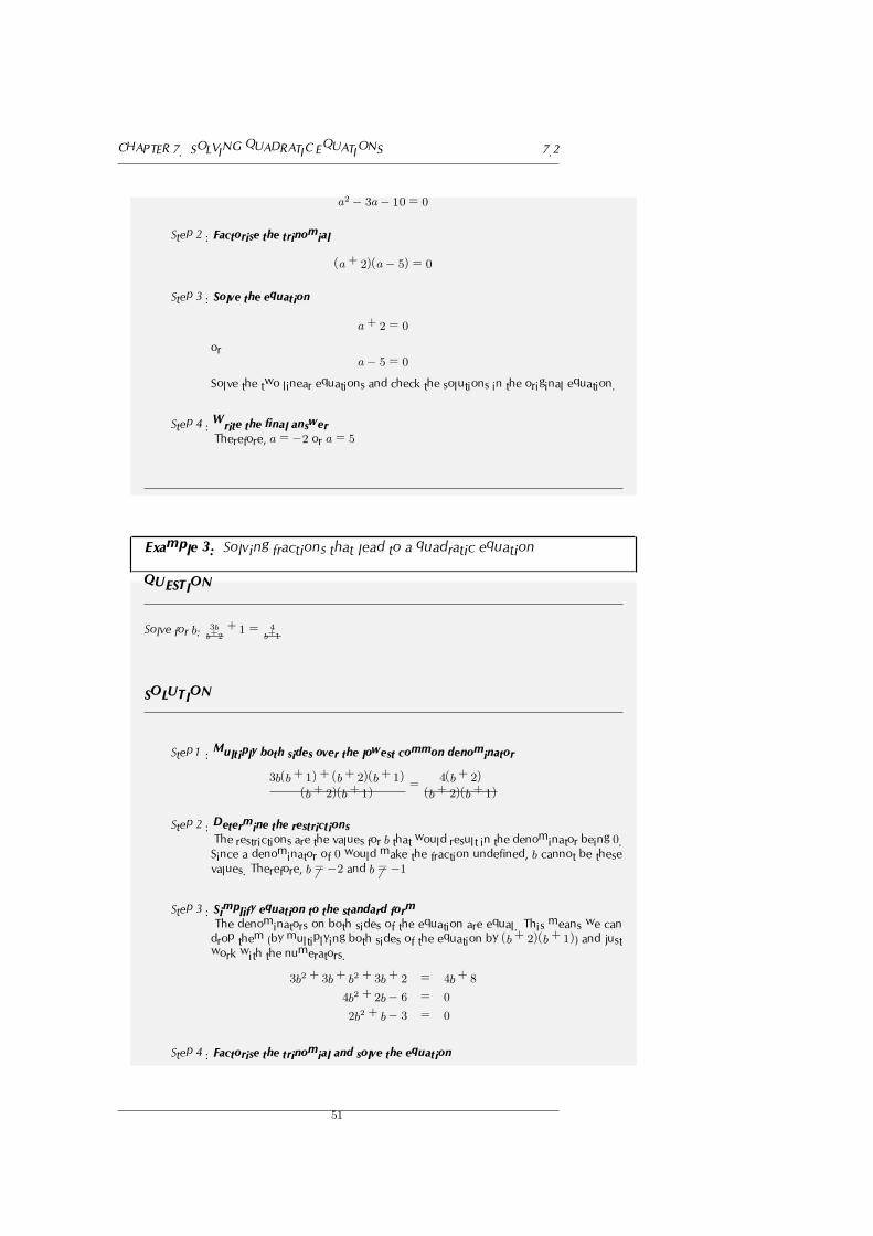
CHAPTER 7. SOLVING QUADRATIC EQUATIONS 7.2
a2 − 3a− 10 = 0
Step 2 : Factorise the trinomial
(a+ 2)(a− 5) = 0
Step 3 : Solve the equation
a+ 2 = 0
or
a− 5 = 0Solve the two linear equations and check the solutions in the original equation.
Step 4 : Write the final answer
Therefore, a = −2 or a = 5
Example 3: Solving fractions that lead to a quadratic equation
QUESTION
Solve for b: 3bb+2
+ 1 = 4b+1
SOLUTION
Step 1 : Multiply both sides over the lowest common denominator
3b(b+ 1) + (b+ 2)(b+ 1)
(b+ 2)(b+ 1)=
4(b+ 2)
(b+ 2)(b+ 1)
Step 2 : Determine the restrictions
The restrictions are the values for b that would result in the denominator being 0.Since a denominator of 0 would make the fraction undefined, b cannot be thesevalues. Therefore, b �= −2 and b �= −1
Step 3 : Simplify equation to the standard form
The denominators on both sides of the equation are equal. This means we can
drop them (by multiplying both sides of the equation by (b + 2)(b + 1)) and just
work with the numerators.
3b2 + 3b+ b2 + 3b+ 2 = 4b+ 8
4b2 + 2b− 6 = 0
2b2 + b− 3 = 0
Step 4 : Factorise the trinomial and solve the equation
51

7.2 CHAPTER 7. SOLVING QUADRATIC EQUATIONS
(2b+ 3)(b− 1) = 0
2b+ 3 = 0 or b− 1 = 0b =
−32
or b = 1
Step 5 : Check solutions in original equation
Both solutions are valid
Therefore, b = −32
or b = 1
Exercise 7 - 1
Solve the following quadratic equations by factorisation. Some answers may be left in surd form.
1. 2y2 − 61 = 101
2. 2y2 − 10 = 0
3. y2 − 4 = 10
4. 2y2 − 8 = 28
5. 7y2 = 28
6. y2 + 28 = 100
7. 7y2 + 14y = 0
8. 12y2 + 24y + 12 = 0
9. 16y2 − 400 = 0
10. y2 − 5y + 6 = 0
11. y2 + 5y − 36 = 0
12. y2 + 2y = 8
13. −y2 − 11y − 24 = 0
14. 13y − 42 = y2
15. y2 + 9y + 14 = 0
16. y2 − 5ky + 4k2 = 0
17. y(2y + 1) = 15
18. 5yy−2
+ 3y+ 2 = −6
y2−2y
19. y−2y+1
= 2y+1y−7
More practice video solutions or help at www.everythingmaths.co.za
(1.) 0185 (2.) 0186 (3.) 0187 (4.) 0188 (5.) 0189 (6.) 018a
(7.) 018b (8.) 018c (9.) 018d (10.) 018e (11.) 018f (12.) 018g
(13.) 018h (14.) 018i (15.) 018j (16.) 018k (17.) 018m (18.) 018n
(19.) 018p
52

CHAPTER 7. SOLVING QUADRATIC EQUATIONS 7.3
7.3 Solution by Completing theSquare
EMBAH
We have seen that expressions of the form:
a2x2 − b2
are known as differences of squares and can be factorised as follows:
(ax− b)(ax+ b).
This simple factorisation leads to another technique to solve quadratic equations known as completing
the square.
We demonstrate with a simple example, by trying to solve for x in:
x2 − 2x− 1 = 0. (7.1)
We cannot easily find factors of this term, but the first two terms look similar to the first two terms of
the perfect square:
(x− 1)2 = x2 − 2x+ 1.However, we can cheat and create a perfect square by adding 2 to both sides of the equation in (7.1)
as:
x2 − 2x− 1 = 0
x2 − 2x− 1 + 2 = 0 + 2
x2 − 2x+ 1 = 2
(x− 1)2 = 2
(x− 1)2 − 2 = 0
Now we know that:
2 = (√2)2
which means that:
(x− 1)2 − 2is a difference of squares. Therefore we can write:
(x− 1)2 − 2 = [(x− 1)−√2][(x− 1) +
√2] = 0.
The solution to x2 − 2x− 1 = 0 is then:
(x− 1)−√2 = 0
or
(x− 1) +√2 = 0.
This means x = 1 +√2 or x = 1−
√2. This example demonstrates the use of completing the square
to solve a quadratic equation.
Method: Solving Quadratic Equations by Completing the Square
1. Write the equation in the form ax2 + bx+ c = 0. e.g. x2 + 2x− 3 = 0
2. Take the constant over to the right hand side of the equation, e.g. x2 + 2x = 3
3. Make the coefficient of the x2 term = 1, by dividing through by the existing coefficient.
4. Take half the coefficient of the x term, square it and add it to both sides of the equation, e.g. in
x2 + 2x = 3, half of the coefficient of the x term is 1 and 12 = 1. Therefore we add 1 to both
sides to get: x2 + 2x+ 1 = 3 + 1.
53

7.3 CHAPTER 7. SOLVING QUADRATIC EQUATIONS
5. Write the left hand side as a perfect square: (x+ 1)2 − 4 = 0
6. You should then be able to factorise the equation in terms of difference of squares and then solve
for x:
[(x+ 1)− 2][(x+ 1) + 2)] = 0
(x− 1)(x+ 3) = 0
∴ x = 1 or x = −3
Example 4: Solving Quadratic Equations by Completing the Square
QUESTION
Solve by completing the square:
x2 − 10x− 11 = 0
SOLUTION
Step 1 : Write the equation in the form ax2 + bx+ c = 0
x2 − 10x− 11 = 0
Step 2 : Take the constant over to the right hand side of the equation
x2 − 10x = 11
Step 3 : Check that the coefficient of the x2 term is 1.The coefficient of the x2 term is 1.
Step 4 : Take half the coefficient of the x term, square it and add it to both sides
The coefficient of the x term is −10. Therefore, half of the coefficient of the xterm will be
(−10)2
= −5 and the square of it will be (−5)2 = 25. Therefore:
x2 − 10x+ 25 = 11 + 25
Step 5 : Write the left hand side as a perfect square
(x− 5)2 − 36 = 0
Step 6 : Factorise equation as difference of squares
(x− 5)2 − 36 = 0[(x− 5) + 6][(x− 5)− 6] = 0
Step 7 : Solve for the unknown value
54

CHAPTER 7. SOLVING QUADRATIC EQUATIONS 7.3
(x+ 1)(x− 11) = 0
∴ x = −1 or x = 11
Example 5: Solving Quadratic Equations by Completing the Square
QUESTION
Solve by completing the square:
2x2 − 8x− 16 = 0
SOLUTION
Step 1 : Write the equation in the form ax2 + bx+ c = 0
2x2 − 8x− 16 = 0
Step 2 : Take the constant over to the right hand side of the equation
2x2 − 8x = 16
Step 3 : Check that the coefficient of the x2 term is 1.The coefficient of the x2 term is 2. Therefore, divide both sides by 2:
x2 − 4x = 8
Step 4 : Take half the coefficient of the x term, square it and add it to both sides
The coefficient of the x term is −4; (−4)2= −2 and (−2)2 = 4. Therefore:
x2 − 4x+ 4 = 8 + 4
Step 5 : Write the left hand side as a perfect square
(x− 2)2 − 12 = 0
Step 6 : Factorise equation as difference of squares
[(x− 2) +√12][(x− 2)−
√12] = 0
Step 7 : Solve for the unknown value
[x− 2 +√12][x− 2−
√12] = 0
∴ x = 2−√12 or x = 2 +
√12
Step 8 : The last three steps can also be done in a different way
55

7.4 CHAPTER 7. SOLVING QUADRATIC EQUATIONS
Leave the left hand side written as a perfect square
(x− 2)2 = 12
Step 9 : Take the square root on both sides of the equation
x− 2 = ±√12
Step 10 : Solve for xTherefore x = 2−
√12 or x = 2 +
√12
Compare to answer in step 7.
See video: VMeyf at www.everythingmaths.co.za
Exercise 7 - 2
Solve the following equations by completing the square:
1. x2 + 10x− 2 = 0
2. x2 + 4x+ 3 = 0
3. x2 + 8x− 5 = 0
4. 2x2 + 12x+ 4 = 0
5. x2 + 5x+ 9 = 0
6. x2 + 16x+ 10 = 0
7. 3x2 + 6x− 2 = 0
8. z2 + 8z − 6 = 0
9. 2z2 − 11z = 0
10. 5 + 4z − z2 = 0
More practice video solutions or help at www.everythingmaths.co.za
(1.) 018q (2.) 018r (3.) 018s (4.) 018t (5.) 018u (6.) 018v
(7.) 018w (8.) 018x (9.) 018y (10.) 018z
7.4 Solution by the QuadraticFormula
EMBAI
It is not always possible to solve a quadratic equation by factorising and sometimes it is lengthy and
tedious to solve a quadratic equation by completing the square. In these situations, you can use the
quadratic formula that gives the solutions to any quadratic equation.
56

CHAPTER 7. SOLVING QUADRATIC EQUATIONS 7.4
Consider the general form of the quadratic function:
f(x) = ax2 + bx+ c.
Factor out the a to get:
f(x) = a
�
x2 +b
ax+
c
a
�
. (7.2)
Now we need to do some detective work to figure out how to turn (7.2) into a perfect square plus some
extra terms. We know that for a perfect square:
(m+ n)2 = m2 + 2mn+ n2
and
(m− n)2 = m2 − 2mn+ n2
The key is the middle term on the right hand side, which is 2× the first term × the second term of the
left hand side. In (7.2), we know that the first term is x so 2× the second term is ba. This means that
the second term is b2a. So,
�
x+b
2a
�2
= x2 + 2b
2ax+
�
b
2a
�2
.
In general if you add a quantity and subtract the same quantity, nothing has changed. This means if we
add and subtract�
b2a
�2from the right hand side of Equation (7.2) we will get:
f(x) = a
�
x2 +b
ax+
c
a
�
(7.3)
= a
�
x2 +b
ax+
�
b
2a
�2
−�
b
2a
�2
+c
a
�
(7.4)
= a
�
�
x+
�
b
2a
��2
−�
b
2a
�2
+c
a
�
(7.5)
= a
�
x+
�
b
2a
��2
− b2
4a+ c (7.6)
We set f(x) = 0 to find its roots, which yields:
a
�
x+b
2a
�2
=b2
4a− c (7.7)
Now dividing by a and taking the square root of both sides gives the expression
x+b
2a= ±
�
b2
4a2− c
a(7.8)
Finally, solving for x implies that
x = − b
2a±
�
b2
4a2− c
a
= − b
2a±
�
b2 − 4ac4a2
which can be further simplified to:
x =−b±
√b2 − 4ac2a
(7.9)
These are the solutions to the quadratic equation. Notice that there are two solutions in general, but
these may not always exists (depending on the sign of the expression b2 − 4ac under the square root).These solutions are also called the roots of the quadratic equation.
57

7.4 CHAPTER 7. SOLVING QUADRATIC EQUATIONS
Example 6: Using the quadratic formula
QUESTION
Find the roots of the function f(x) = 2x2 + 3x− 7.
SOLUTION
Step 1 : Determine whether the equation can be factorised
The expression cannot be factorised. Therefore, the general quadratic formula
must be used.
Step 2 : Identify the coefficients in the equation for use in the formula
From the equation:
a = 2
b = 3
c = −7
Step 3 : Apply the quadratic formula
Always write down the formula first and then substitute the values of a, b and c.
x =−b±
√b2 − 4ac2a
(7.10)
=−(3)±
�
(3)2 − 4(2)(−7)2(2)
(7.11)
=−3±
√65
4(7.12)
=−3±
√65
4(7.13)
Step 4 : Write the final answer
The two roots of f(x) = 2x2 + 3x− 7 are x = −3+√65
4and −3−
√65
4.
Example 7: Using the quadratic formula but no solution
QUESTION
Find the solutions to the quadratic equation x2 − 5x+ 8 = 0.
58

CHAPTER 7. SOLVING QUADRATIC EQUATIONS 7.4
SOLUTION
Step 1 : Determine whether the equation can be factorised
The expression cannot be factorised. Therefore, the general quadratic formula
must be used.
Step 2 : Identify the coefficients in the equation for use in the formula
From the equation:
a = 1
b = −5c = 8
Step 3 : Apply the quadratic formula
x =−b±
√b2 − 4ac2a
(7.14)
=−(−5)±
�
(−5)2 − 4(1)(8)2(1)
(7.15)
=5±
√−7
2(7.16)
(7.17)
Step 4 : Write the final answer
Since the expression under the square root is negative these are not real solutions
(√−7 is not a real number). Therefore there are no real solutions to the quadratic
equation x2 − 5x + 8 = 0. This means that the graph of the quadratic function
f(x) = x2 − 5x + 8 has no x-intercepts, but that the entire graph lies above the
x-axis.
See video: VMezc at www.everythingmaths.co.za
Exercise 7 - 3
Solve for t using the quadratic formula.
1. 3t2 + t− 4 = 0
2. t2 − 5t+ 9 = 0
3. 2t2 + 6t+ 5 = 0
4. 4t2 + 2t+ 2 = 0
5. −3t2 + 5t− 8 = 0
6. −5t2 + 3t− 3 = 0
7. t2 − 4t+ 2 = 0
59

7.4 CHAPTER 7. SOLVING QUADRATIC EQUATIONS
8. 9t2 − 7t− 9 = 0
9. 2t2 + 3t+ 2 = 0
10. t2 + t+ 1 = 0
More practice video solutions or help at www.everythingmaths.co.za
(1.) 0190 (2.) 0191 (3.) 0192 (4.) 0193 (5.) 0194 (6.) 0195
(7.) 0196 (8.) 0197 (9.) 0198 (10.) 0199
Tip
• In all the ex-amples done sofar, the solutionswere left in surdform. Answerscan also begiven in decimalform, using thecalculator. Readthe instructionswhen answeringquestions in a testor exam whetherto leave answersin surd form, orin decimal formto an appropri-ate number ofdecimal places.
• Completingthe square as amethod to solvea quadratic equa-tion is only donewhen specificallyasked.
Exercise 7 - 4
Solve the quadratic equations by either factorisation, completing the square or by using the quadratic
formula:
• Always try to factorise first, then use the formula if the trinomial cannot be factorised.
• Do some of them by completing the square and then compare answers to those done using the
other methods.
1. 24y2 + 61y − 8 = 0
2. −8y2 − 16y + 42 = 0
3. −9y2 + 24y − 12 = 0
4. −5y2 + 0y + 5 = 0
5. −3y2 + 15y − 12 = 0
6. 49y2 + 0y − 25 = 0
7. −12y2 + 66y − 72 = 0
8. −40y2 + 58y − 12 = 0
9. −24y2 + 37y + 72 = 0
10. 6y2 + 7y − 24 = 0
11. 2y2 − 5y − 3 = 0
12. −18y2 − 55y − 25 = 0
13. −25y2 + 25y − 4 = 0
14. −32y2 + 24y + 8 = 0
15. 9y2 − 13y − 10 = 0
16. 35y2 − 8y − 3 = 0
17. −81y2 − 99y − 18 = 0
18. 14y2 − 81y + 81 = 0
19. −4y2 − 41y − 45 = 0
20. 16y2 + 20y − 36 = 0
21. 42y2 + 104y + 64 = 0
22. 9y2 − 76y + 32 = 0
23. −54y2 + 21y + 3 = 0
24. 36y2 + 44y + 8 = 0
25. 64y2 + 96y + 36 = 0
26. 12y2 − 22y − 14 = 0
27. 16y2 + 0y − 81 = 0
28. 3y2 + 10y − 48 = 0
29. −4y2 + 8y − 3 = 0
30. −5y2 − 26y + 63 = 0
31. x2 − 70 = 11
32. 2x2 − 30 = 2
33. x2 − 16 = 2− x2
34. 2y2 − 98 = 0
35. 5y2 − 10 = 115
36. 5y2 − 5 = 19− y2
More practice video solutions or help at www.everythingmaths.co.za
(1.) 01zs (2.) 01zt (3.) 01zu (4.) 01zv (5.) 01zw (6.) 01zx
(7.) 01zy (8.) 01zz (9.) 0200 (10.) 0201 (11.) 0202 (12.) 0203
(13.) 0204 (14.) 0205 (15.) 0206 (16.) 0207 (17.) 0208 (18.) 0209
(19.) 020a (20.) 020b (21.) 020c (22.) 020d (23.) 020e (24.) 020f
(25.) 020g (26.) 020h (27.) 020i (28.) 020j (29.) 020k (30.) 020m
(31.) 020n (32.) 020p (33.) 020q (34.) 020r (35.) 020s (36.) 020t
60

CHAPTER 7. SOLVING QUADRATIC EQUATIONS 7.5
7.5 Finding an Equation When YouKnow its Roots
EMBAJ
We have mentioned before that the roots of a quadratic equation are the solutions or answers you get
from solving the quadratic equation. Working back from the answers, will take you to an equation.
Example 8: Find an equation when roots are given
QUESTION
Find an equation with roots 13 and −5
SOLUTION
Step 1 : Write down as the product of two brackets
The step before giving the solutions would be:
(x− 13)(x+ 5) = 0
Notice that the signs in the brackets are opposite of the given roots.
Step 2 : Remove brackets
x2 − 8x− 65 = 0Of course, there would be other possibilities as well when each term on each
side of the equals sign is multiplied by a constant.
Example 9: Fraction roots
QUESTION
Find an equation with roots − 32and 4
SOLUTION
61

7.5 CHAPTER 7. SOLVING QUADRATIC EQUATIONS
Step 1 : Product of two brackets
Notice that if x = − 32then 2x+ 3 = 0
Therefore the two brackets will be:
(2x+ 3)(x− 4) = 0
Step 2 : Remove brackets
The equation is:
2x2 − 5x− 12 = 0
Extension: Theory of Quadratic Equations - Advanced
This section is not in the syllabus, but it gives one a good understanding about some of the
solutions of the quadratic equations.
What is the Discriminant of a QuadraticEquation?
EMBAK
Consider a general quadratic function of the form f(x) = ax2 + bx + c. The discriminant isdefined as:
Δ = b2 − 4ac. (7.18)
This is the expression under the square root in the formula for the roots of this function. We
have already seen that whether the roots exist or not depends on whether this factor Δ is
negative or positive.
The Nature of the Roots EMBAL
Real Roots (Δ ≥ 0)
Consider Δ ≥ 0 for some quadratic function f(x) = ax2 + bx + c. In this case there are
solutions to the equation f(x) = 0 given by the formula
x =−b±
√b2 − 4ac2a
=−b±
√Δ
2a(7.19)
If the expression under the square root is non-negative then the square root exists. These are
the roots of the function f(x).There various possibilities are summarised in the figure below.
62

CHAPTER 7. SOLVING QUADRATIC EQUATIONS 7.5
Δ
Δ < 0 : imaginary roots Δ ≥ 0 : real roots
Δ = 0equal roots
Δ > 0unequal roots
Δ a per-
fect square :
rational roots
Δ not a perfect
square : irra-
tional roots
Equal Roots (Δ = 0)
If Δ = 0, then the roots are equal and, from the formula, these are given by
x = − b
2a(7.20)
Unequal Roots (Δ > 0)
There will be two unequal roots if Δ > 0. The roots of f(x) are rational if Δ is a perfect
square (a number which is the square of a rational number), since, in this case,√Δ is rational.
Otherwise, if Δ is not a perfect square, then the roots are irrational.
Imaginary Roots (Δ < 0)
If Δ < 0, then the solution to f(x) = ax2 + bx+ c = 0 contains the square root of a negativenumber and therefore there are no real solutions. We therefore say that the roots of f(x) areimaginary (the graph of the function f(x) does not intersect the x-axis).
See video: VMfba at www.everythingmaths.co.za
Extension: Theory of Quadratics - advanced exercises
Exercise 7 - 5
1. [IEB, Nov. 2001, HG] Given: x2 + bx− 2 + k(x2 + 3x+ 2) = 0, (k �= −1)(a) Show that the discriminant is given by:
Δ = k2 + 6bk + b2 + 8
(b) If b = 0, discuss the nature of the roots of the equation.
(c) If b = 2, find the value(s) of k for which the roots are equal.
2. [IEB, Nov. 2002, HG] Show that k2x2+2 = kx− x2 has non-real roots for all real values
for k.
3. [IEB, Nov. 2003, HG] The equation x2 + 12x = 3kx2 + 2 has real roots.
(a) Find the largest integral value of k.
(b) Find one rational value of k, for which the above equation has rational roots.
4. [IEB, Nov. 2003, HG] In the quadratic equation px2 + qx+ r = 0, p, q and r are positivereal numbers and form a geometric sequence. Discuss the nature of the roots.
63

7.5 CHAPTER 7. SOLVING QUADRATIC EQUATIONS
5. [IEB, Nov. 2004, HG] Consider the equation:
k =x2 − 42x− 5 where x �= 5
2
(a) Find a value of k for which the roots are equal.
(b) Find an integer k for which the roots of the equation will be rational and unequal.
6. [IEB, Nov. 2005, HG]
(a) Prove that the roots of the equation x2 − (a+ b)x+ ab− p2 = 0 are real for all realvalues of a, b and p.
(b) When will the roots of the equation be equal?
7. [IEB, Nov. 2005, HG] If b and c can take on only the values 1; 2 or 3, determine all pairs(b; c) such that x2 + bx+ c = 0 has real roots.
More practice video solutions or help at www.everythingmaths.co.za
(1.) 019a (2.) 019b (3.) 019c (4.) 019d (5.) 019e (6.) 019f
(7.) 019g
Chapter 7 End of Chapter Exercises
1. Solve: x2 − x− 1 = 0 (Give your answer correct to two decimal places.)
2. Solve: 16(x+ 1) = x2(x+ 1)
3. Solve: y2 + 3 +12
y2 + 3= 7 (Hint: Let y2 + 3 = k and solve for k first and use the
answer to solve y.)
4. Solve for x: 2x4 − 5x2 − 12 = 05. Solve for x:
(a) x(x− 9) + 14 = 0(b) x2 − x = 3 (Show your answer correct to one decimal place.)
(c) x+ 2 =6
x(correct to two decimal places)
(d)1
x+ 1+
2x
x− 1 = 1
6. Solve for x in terms of p by completing the square: x2 − px− 4 = 07. The equation ax2+ bx+ c = 0 has roots x = 2
3and x = −4. Find one set of possible
values for a, b and c.
8. The two roots of the equation 4x2 + px− 9 = 0 differ by 5. Calculate the value of p.9. An equation of the form x2 + bx + c = 0 is written on the board. Saskia and Sven
copy it down incorrectly. Saskia has a mistake in the constant term and obtains
the solutions −4 and 2. Sven has a mistake in the coefficient of x and obtains the
solutions 1 and −15. Determine the correct equation that was on the board.
10. Bjorn stumbled across the following formula to solve the quadratic equation ax2 +bx+ c = 0 in a foreign textbook.
x =2c
−b±√b2 − 4ac
64

CHAPTER 7. SOLVING QUADRATIC EQUATIONS 7.5
(a) Use this formula to solve the equation:
2x2 + x− 3 = 0
(b) Solve the equation again, using factorisation, to see if the formula works for this
equation.
(c) Trying to derive this formula to prove that it always works, Bjorn got stuck along
the way. His attempt his shown below:
ax2 + bx+ c = 0
a+b
x+
c
x2= 0 Divided by x2 where x �= 0
c
x2+
b
x+ a = 0 Rearranged
1
x2+
b
cx+
a
c= 0 Divided by c where c �= 0
1
x2+
b
cx= −a
cSubtracted
a
cfrom both sides
∴1
x2+
b
cx+ . . . Got stuck
Complete his derivation.
More practice video solutions or help at www.everythingmaths.co.za
(1.) 019h (2.) 019i (3.) 019j (4.) 019k (5.) 019m (6.) 019n
(7.) 019p (8.) 019q (9.) 019r (10.) 019s
65

Solving QuadraticInequalities 8
8.1 Introduction EMBAM
Now that you know how to solve quadratic equations, you are ready to move on to solving quadratic
inequalities. As with linear inequalities (which were covered in Grade 10) your solutions will be
intervals on the number line, rather than single numbers.
See introductory video: VMfdy at www.everythingmaths.co.za
8.2 Quadratic Inequalities EMBAN
A quadratic inequality is an inequality in one of the following forms:
ax2 + bx+ c > 0
ax2 + bx+ c ≥ 0
ax2 + bx+ c < 0
ax2 + bx+ c ≤ 0
Solving a quadratic inequality corresponds to working out in what region the graph of a quadratic
function lies above or below the x-axis.
Example 1: Quadratic Inequality
QUESTION
Solve the inequality 4x2 − 4x+ 1 ≤ 0 and interpret the solution graphically.
SOLUTION
Step 1 : Factorise the quadratic
Let f(x) = 4x2 − 4x + 1. Factorising this quadratic function gives f(x) =(2x− 1)2.
Step 2 : Re-write the original equation with factors
66

CHAPTER 8. SOLVING QUADRATIC INEQUALITIES 8.2
(2x− 1)2 ≤ 0
Step 3 : Solve the equation
f(x) = 0 only when x = 12.
Step 4 : Write the final answer
This means that the graph of f(x) = 4x2 − 4x + 1 touches the x-axis at x = 12,
but there are no regions where the graph is below the x-axis.
Step 5 : Graphical interpretation of solution
−2 −1 0 1 2
�
x = 12
Example 2: Solving Quadratic Inequalities
QUESTION
Find all the solutions to the inequality x2 − 5x+ 6 ≥ 0.
SOLUTION
Step 1 : Factorise the quadratic
The factors of x2 − 5x+ 6 are (x− 3)(x− 2).
Step 2 : Write the inequality with the factors
x2 − 5x+ 6 ≥ 0
(x− 3)(x− 2) ≥ 0
Step 3 : Determine which ranges correspond to the inequality
We need to figure out which values of x satisfy the inequality. From the answers
we have five regions to consider.
� �
1 2 3 4
A B C D E
Step 4 : Determine whether the function is negative or positive in each of the regions
Let f(x) = x2 − 5x + 6. For each region, choose any point in the region and
evaluate the function.
67

8.2 CHAPTER 8. SOLVING QUADRATIC INEQUALITIES
f(x) sign of f(x)Region A x < 2 f(1) = 2 +
Region B x = 2 f(2) = 0 +
Region C 2 < x < 3 f(2,5) = −2,5 -
Region D x = 3 f(3) = 0 +
Region E x > 3 f(4) = 2 +
We see that the function is positive for x ≤ 2 and x ≥ 3.
Step 5 : Write the final answer and represent on a number line
We see that x2 − 5x+ 6 ≥ 0 is true for x ≤ 2 and x ≥ 3.
� �
1 2 3 4
Example 3: Solving Quadratic Inequalities
QUESTION
Solve the quadratic inequality −x2 − 3x+ 5 > 0.
SOLUTION
Step 1 : Determine how to approach the problem
Let f(x) = −x2 − 3x + 5. f(x) cannot be factorised so, use the quadratic
formula to determine the roots of f(x). The x-intercepts are solutions to the
quadratic equation
−x2 − 3x+ 5 = 0
x2 + 3x− 5 = 0
∴ x =−3±
�
(3)2 − 4(1)(−5)2(1)
=−3±
√29
2
x1 =−3−
√29
2= −4,2
x2 =−3 +
√29
2= 1,2
Step 2 : Determine which ranges correspond to the inequality
We need to figure out which values of x satisfy the inequality. From the answers
we have five regions to consider.
� �A B
−4,2C D
1,2
E
68

CHAPTER 8. SOLVING QUADRATIC INEQUALITIES 8.2
Step 3 : Determine whether the function is negative or positive in each of the regions
We can use another method to determine the sign of the function over differ-
ent regions, by drawing a rough sketch of the graph of the function. We know
that the roots of the function correspond to the x-intercepts of the graph. Let
g(x) = −x2−3x+5. We can see that this is a parabola with a maximum turning
point that intersects the x-axis at −4,2 and 1,2.
1
2
3
4
5
6
7
−11−1−2−3−4
x1 x2
It is clear that g(x) > 0 for x1 < x < x2
Step 4 : Write the final answer and represent the solution graphically
−x2 − 3x+ 5 > 0 for −4,2 < x < 1,2
−4,2 1,2
When working with an inequality in which the variable is in the denominator, a different approach is
needed.
Example 4: Non-linear inequality with the variable in the denominator
QUESTION
Solve2
x+ 3≤ 1
x− 3
SOLUTION
69

8.2 CHAPTER 8. SOLVING QUADRATIC INEQUALITIES
Step 1 : Subtract 1x−3
from both sides
2
x+ 3− 1
x− 3 ≤ 0
Step 2 : Simplify the fraction by finding LCD
2(x− 3)− (x+ 3)(x+ 3)(x− 3) ≤ 0
x− 9(x+ 3)(x− 3) ≤ 0
Step 3 : Draw a number line for the inequality
undef undef
−3 3 9
+0−+−
We see that the expression is negative for x < −3 or 3 < x ≤ 9.
Step 4 : Write the final answer
x < −3 or 3 < x ≤ 9
See video: VMfeu at www.everythingmaths.co.za
Chapter 8 End of Chapter Exercises
Solve the following inequalities and show your answer on a number line:
1. Solve: x2 − x < 12.
2. Solve: 3x2 > −x+ 4
3. Solve: y2 < −y − 24. Solve: −t2 + 2t > −35. Solve: s2 − 4s > −66. Solve: 0 ≥ 7x2 − x+ 8
7. Solve: 0 ≥ −4x2 − x
8. Solve: 0 ≥ 6x2
9. Solve: 2x2 + x+ 6 ≤ 0
10. Solve for x if:x
x− 3 < 2 and x �= 3.
11. Solve for x if:4
x− 3 ≤ 1.
70

CHAPTER 8. SOLVING QUADRATIC INEQUALITIES 8.2
12. Solve for x if:4
(x− 3)2 < 1.
13. Solve for x:2x− 2x− 3 > 3
14. Solve for x:−3
(x− 3)(x+ 1) < 0
15. Solve: (2x− 3)2 < 4
16. Solve: 2x ≤ 15− x
x
17. Solve for x:x2 + 3
3x− 2 ≤ 0
18. Solve: x− 2 ≥ 3
x
19. Solve for x:x2 + 3x− 45 + x4
≤ 0
20. Determine all real solutions:x− 23− x
≥ 1
More practice video solutions or help at www.everythingmaths.co.za
(1.) 019t (2.) 019u (3.) 019v (4.) 019w (5.) 019x (6.) 019y
(7.) 019z (8.) 01a0 (9.) 01a1 (10.) 01a2 (11.) 01a3 (12.) 01a4
(13.) 01a5 (14.) 01a6 (15.) 01a7 (16.) 01a8 (17.) 01a9 (18.) 01aa
(19.) 01ab (20.) 01ac
71

Solving SimultaneousEquations 9
9.1 Introduction EMBAO
In Grade 10, you learnt how to solve sets of simultaneous equations where both equations were linear
(i.e. had the highest power equal to 1). In this chapter, you will learn how to solve sets of simultaneous
equations where one is linear and one is quadratic. As in Grade 10, the solution will be found both
algebraically and graphically.
The only difference between a system of linear simultaneous equations and a system of simultaneous
equations with one linear and one quadratic equation, is that the second system will have at most two
solutions.
An example of a system of simultaneous equations with one linear equation and one quadratic equa-
tion is:
y − 2x = −4 (9.1)
x2 + y = 4
See introductory video: VMfwh at www.everythingmaths.co.za
9.2 Graphical Solution EMBAP
The method of graphically finding the solution to one linear and one quadratic equation is identical to
systems of linear simultaneous equations.
Method: Graphical solution to a system ofsimultaneous equations with one linear andone quadratic equation
EMBAQ
1. Make y the subject of each equation.
2. Draw the graphs of each equation as defined above.
3. The solution of the set of simultaneous equations is given by the intersection points of the two
graphs.
For this example, making y the subject of each equation, gives:
y = 2x− 4y = 4− x2
Plotting the graph of each equation, gives a straight line for the first equation and a parabola for the
second equation.
72

CHAPTER 9. SOLVING SIMULTANEOUS EQUATIONS 9.2
2
4
6
−2−4−6−8
−10−12−14
2 4 6−2−4−6
y=2x−4
y=
4−
x2
(−4;−12)
(2; 0)
�
�
The parabola and the straight line intersect at two points: (2; 0) and (−4;−12). Therefore, the solutionsto the system of equations in (9.1) is x = 2; y = 0 and x = −4; y = 12
Example 1: Simultaneous Equations
QUESTION
Solve graphically:
y − x2 + 9 = 0
y + 3x− 9 = 0
SOLUTION
Step 1 : Make y the subject of the equation
For the first equation:
y − x2 + 9 = 0
y = x2 − 9
and for the second equation:
y + 3x− 9 = 0
y = −3x+ 9
Step 2 : Draw the graphs corresponding to each equation.
73

9.3 CHAPTER 9. SOLVING SIMULTANEOUS EQUATIONS
10
20
30
40
2 4 6 8−2−4−6−8
y = −3x+9
y=x2−9
�
�
(−6; 27)
(3; 0)
Step 3 : Find the intersection of the graphs.
The graphs intersect at (−6; 27) and at (3; 0).
Step 4 : Write the solution of the system of simultaneous equations as given by the
intersection of the graphs.
The first solution is x = −6 and y = 27. The second solution is x = 3 and y = 0.
Exercise 9 - 1
Solve the following systems of equations graphically. Leave your answer in surd form, where appropri-
ate.
1. b2 − 1− a = 0; a+ b− 5 = 0
2. x+ y − 10 = 0;x2 − 2− y = 0
3. 6− 4x− y = 0; 12− 2x2 − y = 0
4. x+ 2y − 14 = 0;x2 + 2− y = 0
5. 2x+ 1− y = 0; 25− 3x− x2 − y = 0
More practice video solutions or help at www.everythingmaths.co.za
(1.) 01ad (2.) 01ae (3.) 01af (4.) 01ag (5.) 01ah
9.3 Algebraic Solution EMBAR
The algebraic method of solving simultaneous equations is by substitution.
74

CHAPTER 9. SOLVING SIMULTANEOUS EQUATIONS 9.3
For example the solution of
y − 2x = −4 (9.2)
x2 + y = 4 (9.3)
is:
In (9.2)
y = 2x− 4 (9.4)
Substitute (9.4) into (9.3):
x2 + (2x− 4) = 4
x2 + 2x− 8 = 0
Factorise to get:
(x+ 4)(x− 2) = 0
∴ x = −4 and x = 2
Substitute the values of x into (9.4) to find y:
y = 2(−4)− 4 y = 2(2)− 4y = −12 y = 0
(−4;−12) (2; 0)
As expected, these solutions are identical to those obtained by the graphical solution.
Example 2: Simultaneous Equations
QUESTION
Solve algebraically:
y − x2 + 9 = 0 (9.5)
y + 3x− 9 = 0 (9.6)
SOLUTION
Step 1 : Make y the subject of the linear equation
In (9.5):
y + 3x− 9 = 0
y = −3x+ 9 (9.7)
Step 2 : Substitute into the quadratic equation
75

9.3 CHAPTER 9. SOLVING SIMULTANEOUS EQUATIONS
Substitute (9.7) into (9.5):
(−3x+ 9)− x2 + 9 = 0
x2 + 3x− 18 = 0
Factorise to get:
(x+ 6)(x− 3) = 0
∴ x = −6 and x = 3
Step 3 : Substitute the values for x into the first equation to calculate the corresponding
y-values.Substitute x into 9.5:
y = −3(−6) + 9 y = −3(3) + 9= 27 = 0
(−6; 27) (3; 0)
Step 4 : Write the solution of the system of simultaneous equations.
The first solution is x = −6 and y = 27. The second solution is x = 3 and y = 0.
Chapter 9 End of Chapter Exercises
Solve the following systems of equations algebraically. Leave your answer in surd form,
where appropriate.
1. a+ b = 5 ; a− b2 + 3b− 5 = 02. a− b+ 1 = 0 ; a− b2 + 5b− 6 = 03. a− (2b+2)
4= 0 a− 2b2 + 3b+ 5 = 0
4. a+ 2b− 4 = 0 ; a− 2b2 − 5b+ 3 = 05. a− 2 + 3b = 0 ; a− 9 + b2 = 0
6. a− b− 5 = 0 ; a− b2 = 0
7. a− b− 4 = 0 ; a+ 2b2 − 12 = 08. a+ b− 9 = 0 ; a+ b2 − 18 = 09. a− 3b+ 5 = 0 ; a+ b2 − 4b = 0
10. a+ b− 5 = 0 ; a− b2 + 1 = 0
11. a− 2b− 3 = 0 ; a− 3b2 + 4 = 012. a− 2b = 0 ; a− b2 − 2b+ 3 = 013. a− 3b = 0 ; a− b2 + 4 = 0
14. a− 2b− 10 = 0 ; a− b2 − 5b = 015. a− 3b− 1 = 0 ; a− 2b2 − b+ 3 = 0
16. a− 3b+ 1 = 0 ; a− b2 = 0
17. a+ 6b− 5 = 0 ; a− b2 − 8 = 0
76

CHAPTER 9. SOLVING SIMULTANEOUS EQUATIONS 9.3
18. a− 2b+ 1 = 0 ; a− 2b2 − 12b+ 4 = 019. 2a+ b− 2 = 0 ; 8a+ b2 − 8 = 020. a+ 4b− 19 = 0 ; 8a+ 5b2 − 101 = 021. a+ 4b− 18 = 0 ; 2a+ 5b2 − 57 = 0
More practice video solutions or help at www.everythingmaths.co.za
(1.) 020u (2.) 020v (3.) 020w (4.) 020x (5.) 020y (6.) 020z
(7.) 0210 (8.) 0211 (9.) 0212 (10.) 0213 (11.) 0214 (12.) 0215
(13.) 0216 (14.) 0217 (15.) 0218 (16.) 0219 (17.) 021a (18.) 021b
(19.) 021c (20.) 021d (21.) 021e
77

Mathematical Models 10
10.1 Introduction EMBAS
Up until now, you have only learnt how to solve equations and inequalities, but there has not been
much application of what you have learnt. This chapter builds on this knowledge and introduces you
to the idea of a mathematical model, which uses mathematical concepts to solve real-world problems.
See introductory video: VMfjh at www.everythingmaths.co.za
10.2 Mathematical Models EMBAT
DEFINITION: Mathematical Model
A mathematical model is a method of using the mathematical language to describe
the behaviour of a physical system. Mathematical models are used particularly in the
natural sciences and engineering disciplines (such as physics, biology, and electrical
engineering) but also in the social sciences (such as economics, sociology and political
science); physicists, engineers, computer scientists, and economists use mathematical
models most extensively.
A mathematical model is an equation (or a set of equations for the more difficult problems) that de-
scribes a particular situation. For example, if Anna receives R3 for each time she helps her mother
wash the dishes and R5 for each time she helps her father cut the grass, how much money will Anna
earn if she helps her mother to wash the dishes five times and helps her father to wash the car twice?
The first step to modelling is to write the equation, that describes the situation. To calculate how much
Anna will earn we see that she will earn :
5 × R3 for washing the dishes
+ 2 × R5 for cutting the grass
= R15 + R10
= R25
If however, we ask: ”What is the equation if Anna helps her mother x times and her father y times?”,
then we have:
Total earned = (x× R3) + (y × R5)
78

CHAPTER 10. MATHEMATICAL MODELS 10.3
10.3 Real-World Applications EMBAU
Some examples of where mathematical models are used in the real-world are:
1. To model population growth
2. To model effects of air pollution
3. To model effects of global warming
4. In computer games
5. In the sciences (e.g. physics, chemistry, biology) to understand how the natural world works
6. In simulators that are used to train people in certain jobs, like pilots, doctors and soldiers
7. In medicine to track the progress of a disease
Activity: Simple Models
In order to get used to the idea of mathematical models, try the following simple models.
Write an equation that describes the following real-world situations, mathematically:
1. Jack and Jill both have colds. Jack sneezes twice for each sneeze of Jill’s. If Jill sneezes xtimes, write an equation describing how many times they both sneezed?
2. It rains half as much in July as it does in December. If it rains y mm in July, write an
expression relating the rainfall in July and December.
3. Zane can paint a room in 4 hours. Billy can paint a room in 2 hours. How long will it
take both of them to paint a room together?
4. 25 years ago, Arthur was 5 more than 13as old as Lee was. Today, Lee is 26 less than
twice Arthur’s age. How old is Lee?
5. Kevin has played a few games of ten-pin bowling. In the third game, Kevin scored 80more than in the second game. In the first game Kevin scored 110 less than the third
game. His total score for the first two games was 208. If he wants an average score of
146, what must he score on the fourth game?
6. Erica has decided to treat her friends to coffee at the Corner Coffee House. Erica paid
R54,00 for four cups of cappuccino and three cups of filter coffee. If a cup of cappuccinocosts R3,00 more than a cup of filter coffee, calculate how much each type of coffee
costs?
7. The product of two integers is 95. Find the integers if their total is 24.
79

10.3 CHAPTER 10. MATHEMATICAL MODELS
Example 1: Mathematical Modelling of Falling Objects
QUESTION
When an object is dropped or thrown downward, the distance, d, that it falls in time, t isdescribed by the following equation:
s = 5t2 + v0t
In this equation, v0 is the initial velocity, in m · s−1. Distance is measured in meters and time
is measured in seconds. Use the equation to find how far an object will fall in 2 s if it isthrown downward at an initial velocity of 10 m · s−1.
SOLUTION
Step 1 : Identify what is given for each problem
We are given an expression to calculate distance travelled by a falling object in
terms of initial velocity and time. We are also given the initial velocity and time
and are required to calculate the distance travelled.
Step 2 : List all known and unknown information
• v0 = 10 m · s−1
• t = 2 s
• s =? m
Step 3 : Substitute values into expression
s = 5t2 + v0t
= 5(2)2 + (10)(2)
= 5(4) + 20
= 20 + 20
= 40
Step 4 : Write the final answer
The object will fall 40 m in 2 s if it is thrown downward at an initial velocity of
10 m · s−1.
80

CHAPTER 10. MATHEMATICAL MODELS 10.3
Example 2: Another Mathematical Modelling of Falling Objects
QUESTION
When an object is dropped or thrown downward, the distance, d, that it falls in time, t isdescribed by the following equation:
s = 5t2 + v0t
In this equation, v0 is the initial velocity, in m · s−1. Distance is measured in meters and time
is measured in seconds. Use the equation find how long it takes for the object to reach the
ground if it is dropped from a height of 2000m. The initial velocity is 0 m · s−1.
SOLUTION
Step 1 : Identify what is given for each problem
We are given an expression to calculate distance travelled by a falling object
in terms of initial velocity and time. We are also given the initial velocity and
distance travelled and are required to calculate the time it takes the object to
travel the distance.
Step 2 : List all known and unknown information
• v0 = 0m · s−1
• t =? s
• s = 2000 m
Step 3 : Substitute values into expression
s = 5t2 + v0t
2000 = 5t2 + (0)(2)
2000 = 5t2
t2 =2000
5= 400
∴ t = 20 s
Step 4 : Write the final answer
The object will take 20 s to reach the ground if it is dropped from a height of
2 000 m.
Activity: Mathematical Modelling
The graph below shows how the distance travelled by a car depends on time. Use the
graph to answer the following questions.
81

10.3 CHAPTER 10. MATHEMATICAL MODELS
0
100
200
300
400
0 10 20 30 40
Time (s)
Distance
(m)
1. How far does the car travel in 20 s?
2. How long does it take the car to travel 300 m?
Example 3: More Mathematical Modelling
QUESTION
A researcher is investigating the number of trees in a forest over a period of n years. After
investigating numerous data, the following data model emerged:
Year Number of trees (in hundreds)
1 1
2 3
3 9
4 27
1. How many trees, in hundreds, are there in the sixth year if this pattern is continued?
2. Determine an algebraic expression that describes the number of trees in the nth year inthe forest.
3. Do you think this model, which determines the number of trees in the forest, will con-
tinue indefinitely? Give a reason for your answer.
SOLUTION
Step 1 : Find the pattern
The pattern is 30; 31; 32; 33; . . .Therefore, three to the power one less than the year.
Step 2 : Trees in year 6
Year 6 : 35 hundred = 243 hundred = 24300
Step 3 : Algebraic expression for year n
Number of trees = 3n−1hundred
82

CHAPTER 10. MATHEMATICAL MODELS 10.3
Step 4 : Conclusion
No, the number of trees will not increase indefinitely. The number of trees will
increase for some time. Yet, eventually the number of trees will not increase
any more. It will be limited by factors such as the limited amount of water and
nutrients available in the ecosystem.
Example 4: Setting up an equation
QUESTION
Currently the subscription to a gym for a single member is R1 000 annually while familymembership is R1 500. The gym is considering raising all memberships fees by the same
amount. If this is done then the single membership will cost 57of the family membership.
Determine the proposed increase.
SOLUTION
Step 1 : Summarise the information in a table
Let the proposed increase be x.
Now After increase
Single 1 000 1 000 + x
Family 1 500 1 500 + x
Step 2 : Set up an equation
1 000 + x =5
7(1 500 + x)
Step 3 : Solve the equation.
7 000 + 7x = 7 500 + 5x
2x = 500
x = 250
Step 4 : Write down the answer
Therefore the increase is R250.
83

10.3 CHAPTER 10. MATHEMATICAL MODELS
Extension: Simulations
A simulation is an attempt to model a real-life situation on a computer so that it can be stud-
ied to see how the system works. By changing variables, predictions may be made about the
behaviour of the system. Simulation is used in many contexts, including the modelling of nat-
ural systems or human systems in order to gain insight into their functioning. Other contexts
include simulation of technology for performance optimisation, safety engineering, testing,
training and education. Simulation can be used to show the eventual real effects of alternative
conditions and courses of action.
Simulation in education Simulations in education are somewhat like training simulations. They
focus on specific tasks. In the past, video has been used for teachers and education students to
observe, problem solve and role play; however, a more recent use of simulations in education
is that of animated narrative vignettes (ANV). ANVs are cartoon-like video narratives of hypo-
thetical and reality-based stories involving classroom teaching and learning. ANVs have been
used to assess knowledge, problem solving skills and dispositions of children and pre-service
and in-service teachers.
Chapter 10 End of Chapter Exercises
1. When an object is dropped or thrown downward, the distance, d, that it falls in time,t, is described by the following equation:
s = 5t2 + v0t
In this equation, v0 is the initial velocity, in m · s−1. Distance is measured in meters
and time is measured in seconds. Use the equation to find how long it takes a tennis
ball to reach the ground if it is thrown downward from a hot-air balloon that is 500 mhigh. The tennis ball is thrown at an initial velocity of 5 m · s−1.
2. The table below lists the times that Sheila takes to walk the given distances.
Time (minutes) 5 10 15 20 25 30
Distance (km) 1 2 3 4 5 6
Plot the points.
If the relationship between the distances and times is linear, find the equation of the
straight line, using any two points. Then use the equation to answer the following
questions:
(a) How long will it take Sheila to walk 21 km?
(b) How far will Sheila walk in 7 minutes?
If Sheila were to walk half as fast as she is currently walking, what would the graph
of her distances and times look like?
3. The power P (in watts) supplied to a circuit by a 12 volt battery is given by the
formula P = 12I − 0,5I2 where I is the current in amperes.
(a) Since both power and current must be greater than 0, find the limits of the currentthat can be drawn by the circuit.
(b) Draw a graph of P = 12I − 0,5I2 and use your answer to the first question, to
define the extent of the graph.
(c) What is the maximum current that can be drawn?
84

CHAPTER 10. MATHEMATICAL MODELS 10.3
(d) From your graph, read off how much power is supplied to the circuit when the
current is 10 Amperes. Use the equation to confirm your answer.
(e) At what value of current will the power supplied be a maximum?
4. You are in the lobby of a business building waiting for the lift. You are late for a
meeting and wonder if it will be quicker to take the stairs. There is a fascinating
relationship between the number of floors in the building, the number of people in
the lift and how often it will stop:
If N people get into a lift at the lobby and the number of floors in the
building is F , then the lift can be expected to stop
F − F
�
F − 1F
�N
times.
(a) If the building has 16 floors and there are 9 people who get into the lift, how
many times is the lift expected to stop?
(b) How many people would you expect in a lift, if it stopped 12 times and there are17 floors?
5. A wooden block is made as shown in the diagram. The ends are right-angled triangles
having sides 3x, 4x and 5x. The length of the block is y. The total surface area of theblock is 3600 cm2.
y
3x 4x
5x
Show that
y =300− x2
x
6. A stone is thrown vertically upwards and its height (in metres) above the ground at
time t (in seconds) is given by:
h(t) = 35− 5t2 + 30t
Find its initial height above the ground.
7. After doing some research, a transport company has determined that the rate at which
petrol is consumed by one of its large carriers, travelling at an average speed of x km
per hour, is given by:
P (x) =55
2x+
x
200litres per kilometre
Assume that the petrol costs R4,00 per litre and the driver earns R18,00 per hour
85

10.3 CHAPTER 10. MATHEMATICAL MODELS
(travelling time). Now deduce that the total cost, C, in Rands, for a 2 000 km trip is
given by:
C(x) =256000
x+ 40x
8. During an experiment the temperature T (in degrees Celsius), varies with time t (inhours), according to the formula:
T (t) = 30 + 4t− 1
2t2 t ∈ [1; 10]
(a) Determine an expression for the rate of change of temperature with time.
(b) During which time interval was the temperature dropping?
9. In order to reduce the temperature in a room from 28◦ C, a cooling system is allowed
to operate for 10 minutes. The room temperature, T after t minutes is given in ◦ Cby the formula:
T = 28− 0,008t3 − 0,16t where t ∈ [0; 10]
(a) At what rate (rounded off to two decimal places) is the temperature falling when
t = 4 minutes?
(b) Find the lowest room temperature reached during the 10 minutes for which the
cooling system operates, by drawing a graph.
10. A washing powder box has the shape of a rectangular prism as shown in the diagram
below. The box has a volume of 480 cm3, a breadth of 4 cm and a length of x cm.
Washing powder
Show that the total surface area of the box (in cm2) is given by:
A = 8x+ 960x−1 + 240
More practice video solutions or help at www.everythingmaths.co.za
(1.) 010w (2.) 010x (3.) 010y (4.) 010z (5.) 0110 (6.) 0111
(7.) 0112 (8.) 0113 (9.) 0114 (10.) 0115
86

Quadratic Functions andGraphs 11
11.1 Introduction EMBAV
In Grade 10, you studied graphs of many different forms. Here you will learn how to sketch and
interpret more general quadratic functions.
See introductory video: VMfkg at www.everythingmaths.co.za
11.2 Functions of the Formy = a(x + p)2 + q
EMBAW
This form of the quadratic function is slightly more complex than the form studied in Grade 10, y =ax2+ q. The general shape and position of the graph of the function of the form f(x) = a(x+ p)2+ qis shown in Table 11.1.
1
2
3
−1
−2
−3
1 2 3 4 5−1−2−3−4−5
Figure 11.1: Graph of f(x) = 12(x+ 2)2 − 1
Activity: Functions of the Form y = a(x+ p)2 + q
1. On the same set of axes, plot the following graphs:
(a) a(x) = (x− 2)2(b) b(x) = (x− 1)2(c) c(x) = x2
87
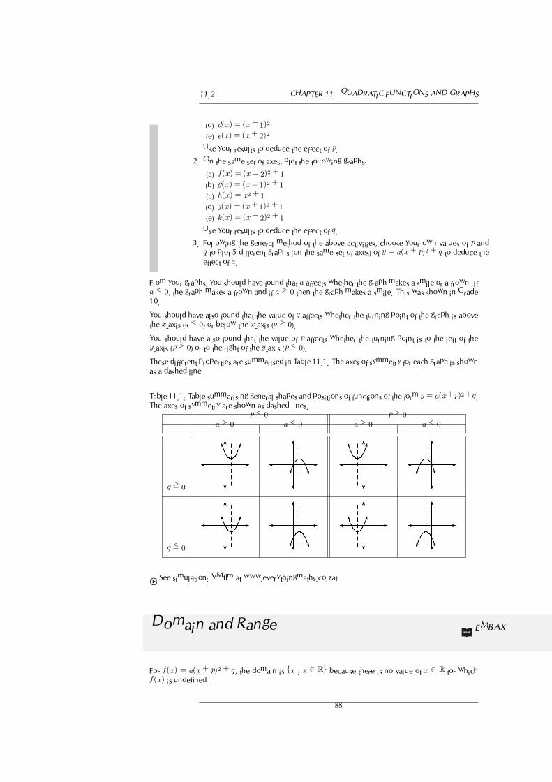
11.2 CHAPTER 11. QUADRATIC FUNCTIONS AND GRAPHS
(d) d(x) = (x+ 1)2
(e) e(x) = (x+ 2)2
Use your results to deduce the effect of p.
2. On the same set of axes, plot the following graphs:
(a) f(x) = (x− 2)2 + 1(b) g(x) = (x− 1)2 + 1(c) h(x) = x2 + 1
(d) j(x) = (x+ 1)2 + 1
(e) k(x) = (x+ 2)2 + 1
Use your results to deduce the effect of q.
3. Following the general method of the above activities, choose your own values of p and
q to plot 5 different graphs (on the same set of axes) of y = a(x + p)2 + q to deduce the
effect of a.
From your graphs, you should have found that a affects whether the graph makes a smile or a frown. If
a < 0, the graph makes a frown and if a > 0 then the graph makes a smile. This was shown in Grade
10.
You should have also found that the value of q affects whether the turning point of the graph is above
the x-axis (q < 0) or below the x-axis (q > 0).
You should have also found that the value of p affects whether the turning point is to the left of the
y-axis (p > 0) or to the right of the y-axis (p < 0).
These different properties are summarised in Table 11.1. The axes of symmetry for each graph is shown
as a dashed line.
Table 11.1: Table summarising general shapes and positions of functions of the form y = a(x+p)2+q.The axes of symmetry are shown as dashed lines.
p < 0 p > 0
a > 0 a < 0 a > 0 a < 0
q ≥ 0
q ≤ 0
See simulation: VMflm at www.everythingmaths.co.za)
Domain and Range EMBAX
For f(x) = a(x + p)2 + q, the domain is {x : x ∈ R} because there is no value of x ∈ R for which
f(x) is undefined.
88

CHAPTER 11. QUADRATIC FUNCTIONS AND GRAPHS 11.2
The range of f(x) = a(x+ p)2+ q depends on whether the value for a is positive or negative. We will
consider these two cases separately.
If a > 0 then we have:
(x+ p)2 ≥ 0 (The square of an expression is always positive)
a(x+ p)2 ≥ 0 (Multiplication by a positive number maintains the nature of the inequality)
a(x+ p)2 + q ≥ q
f(x) ≥ q
This tells us that for all values of x, f(x) is always greater than or equal to q. Therefore if a > 0, therange of f(x) = a(x+ p)2 + q is {f(x) : f(x) ∈ [q,∞)}.
Similarly, it can be shown that if a < 0 that the range of f(x) = a(x+p)2+q is {f(x) : f(x) ∈ (−∞,q]}.This is left as an exercise.
For example, the domain of g(x) = (x− 1)2 + 2 is {x : x ∈ R} because there is no value of x ∈ R for
which g(x) is undefined. The range of g(x) can be calculated as follows:
(x− p)2 ≥ 0
(x+ p)2 + 2 ≥ 2
g(x) ≥ 2
Therefore the range is {g(x) : g(x) ∈ [2,∞)}.
Exercise 11 - 1
1. Given the function f(x) = (x− 4)2 − 1. Give the range of f(x).
2. What is the domain of the equation y = 2x2 − 5x− 18?
More practice video solutions or help at www.everythingmaths.co.za
(1.) 0116 (2.) 0117
Intercepts EMBAY
For functions of the form, y = a(x+ p)2 + q, the details of calculating the intercepts with the x and yaxes is given.
The y-intercept is calculated as follows:
y = a(x+ p)2 + q (11.1)
yint = a(0 + p)2 + q (11.2)
= ap2 + q (11.3)
If p = 0, then yint = q.
89

11.2 CHAPTER 11. QUADRATIC FUNCTIONS AND GRAPHS
For example, the y-intercept of g(x) = (x− 1)2 + 2 is given by setting x = 0 to get:
g(x) = (x− 1)2 + 2yint = (0− 1)2 + 2
= (−1)2 + 2= 1 + 2
= 3
The x-intercepts are calculated as follows:
y = a(x+ p)2 + q (11.4)
0 = a(xint + p)2 + q (11.5)
a(xint + p)2 = −q (11.6)
xint + p = ±�
− q
a(11.7)
xint = ±�
− q
a− p (11.8)
However, (11.8) is only valid if − q
a> 0 which means that either q < 0 or a < 0 but not both. This
is consistent with what we expect, since if q > 0 and a > 0 then − q
ais negative and in this case the
graph lies above the x-axis and therefore does not intersect the x-axis. If however, q > 0 and a < 0,then − q
ais positive and the graph is hat shaped with turning point above the x-axis and should have
two x-intercepts. Similarly, if q < 0 and a > 0 then − q
ais also positive, and the graph should intersect
with the x-axis twice.
For example, the x-intercepts of g(x) = (x− 1)2 + 2 are given by setting y = 0 to get:
g(x) = (x− 1)2 + 20 = (xint − 1)2 + 2
−2 = (xint − 1)2
which has no real solutions. Therefore, the graph of g(x) = (x−1)2+2 does not have any x-intercepts.
Exercise 11 - 2
1. Find the x- and y-intercepts of the function f(x) = (x− 4)2 − 1.
2. Find the intercepts with both axes of the graph of f(x) = x2 − 6x+ 8.
3. Given: f(x) = −x2 + 4x− 3. Calculate the x- and y-intercepts of the graph of f .
More practice video solutions or help at www.everythingmaths.co.za
(1.) 0118 (2.) 0119 (3.) 011a
Turning Points EMBAZ
The turning point of the function of the form f(x) = a(x+ p)2 + q is given by examining the range of
the function. We know that if a > 0 then the range of f(x) = a(x+ p)2 + q is {f(x) : f(x) ∈ [q,∞)}and if a < 0 then the range of f(x) = a(x+ p)2 + q is {f(x) : f(x) ∈ (−∞,q]}.
90

CHAPTER 11. QUADRATIC FUNCTIONS AND GRAPHS 11.2
So, if a > 0, then the lowest value that f(x) can take on is q. Solving for the value of x at which
f(x) = q gives:
q = a(x+ p)2 + q
0 = a(x+ p)2
0 = (x+ p)2
0 = x+ p
x = −p
∴ x = −p at f(x) = q. The co-ordinates of the (minimal) turning point are therefore (−p; q).
Similarly, if a < 0, then the highest value that f(x) can take on is q and the co-ordinates of the
(maximal) turning point are (−p; q).
Exercise 11 - 3
1. Determine the turning point of the graph of f(x) = x2 − 6x+ 8.
2. Given: f(x) = −x2 + 4x− 3. Calculate the co-ordinates of the turning point of f .
3. Find the turning point of the following function:
y = 12(x+ 2)2 − 1.
More practice video solutions or help at www.everythingmaths.co.za
(1.) 011b (2.) 011c (3.) 011d
Axes of Symmetry EMBBA
There is only one axis of symmetry for the function of the form f(x) = a(x+ p)2 + q. This axis passesthrough the turning point and is parallel to the y-axis. Since the x-coordinate of the turning point is
x = −p, this is the axis of symmetry.
Exercise 11 - 4
1. Find the equation of the axis of symmetry of the graph y = 2x2 − 5x− 18.
2. Write down the equation of the axis of symmetry of the graph of
y = 3(x− 2)2 + 1.
3. Write down an example of an equation of a parabola where the y-axis is the axis of symmetry.
More practice video solutions or help at www.everythingmaths.co.za
(1.) 011e (2.) 011f (3.) 011g
91

11.2 CHAPTER 11. QUADRATIC FUNCTIONS AND GRAPHS
Sketching Graphs of the Form f (x) = a(x +p)2 + q
EMBBB
In order to sketch graphs of the form f(x) = a(x+ p)2 + q, we need to determine five characteristics:
1. sign of a
2. domain and range
3. turning point
4. y-intercept
5. x-intercept (if appropriate)
For example, sketch the graph of g(x) = − 12(x+ 1)2 − 3. Mark the intercepts, turning point and axis
of symmetry.
Firstly, we determine that a < 0. This means that the graph will have a maximal turning point.
The domain of the graph is {x : x ∈ R} because f(x) is defined for all x ∈ R. The range of the graph
is determined as follows:
(x+ 1)2 ≥ 0
−12(x+ 1)2 ≤ 0
−12(x+ 1)2 − 3 ≤ −3
∴ f(x) ≤ −3
Therefore the range of the graph is {f(x) : f(x) ∈ (−∞,− 3]}.Using the fact that the maximum value that f(x) achieves is −3, then the y-coordinate of the turningpoint is −3. The x-coordinate is determined as follows:
−12(x+ 1)2 − 3 = −3
−12(x+ 1)2 − 3 + 3 = 0
−12(x+ 1)2 = 0
Divide both sides by − 12: (x+ 1)2 = 0
Take square root of both sides: x+ 1 = 0
∴ x = −1
The coordinates of the turning point are: (−1;−3).The y-intercept is obtained by setting x = 0. This gives:
yint = −12(0 + 1)2 − 3
= −12(1)− 3
= −12− 3
= −12− 3
= −72
92

CHAPTER 11. QUADRATIC FUNCTIONS AND GRAPHS 11.2
The x-intercept is obtained by setting y = 0. This gives:
0 = −12(xint + 1)
2 − 3
3 = −12(xint + 1)
2
−3 . 2 = (xint + 1)2
−6 = (xint + 1)2
which has no real solutions. Therefore, there are no x-intercepts.
We also know that the axis of symmetry is parallel to the y-axis and passes through the turning point.
−1
−2
−3
−4
−5
−6
−7
1 2 3 4−1−2−3−4
�
� (0;−3.5)
(−1;−3)
Figure 11.2: Graph of the function f(x) = − 12(x+ 1)2 − 3
See video: VMfkk at www.everythingmaths.co.za
Exercise 11 - 5
1. Draw the graph of y = 3(x − 2)2 + 1 showing all the intercepts with the axes as well as the
coordinates of the turning point.
2. Draw a neat sketch graph of the function defined by y = ax2 + bx+ c if a > 0; b < 0; b2 = 4ac.
More practice video solutions or help at www.everythingmaths.co.za
(1.) 011h (2.) 011i
93

11.2 CHAPTER 11. QUADRATIC FUNCTIONS AND GRAPHS
Writing an Equation of a Shifted Parabola EMBBC
Given a parabola with equation y = x2 − 2x− 3. The graph of the parabola is shifted one unit to the
right. Or else the y-axis shifts one unit to the left i.e. x becomes x − 1. Therefore the new equation
will become:
y = (x− 1)2 − 2(x− 1)− 3= x2 − 2x+ 1− 2x+ 2− 3= x2 − 4x
If the given parabola is shifted 3 units down i.e. y becomes y + 3. The new equation will be:
(Notice the x-axis then moves 3 units upwards)
y + 3 = x2 − 2x− 3y = x2 − 2x− 6
Chapter 11 End of Chapter Exercises
1. Show that if a < 0, then the range of f(x) = a(x+p)2+q is {f(x) : f(x) ∈ (−∞,q]}.2. If (2; 7) is the turning point of f(x) = −2x2−4ax+k, find the values of the constants
a and k.
3. The graph in the figure is represented by the equation f(x) = ax2 + bx. The coordi-nates of the turning point are (3; 9). Show that a = −1 and b = 6.
� (3; 9)
4. Given: y = x2 − 2x+ 3. Give the equation of the new graph originating if:
(a) The graph of f is moved three units to the left.
(b) The x-axis is moved down three units.
5. A parabola with turning point (−1;−4) is shifted vertically by 4 units upwards. What
are the coordinates of the turning point of the shifted parabola?
94

CHAPTER 11. QUADRATIC FUNCTIONS AND GRAPHS 11.2
More practice video solutions or help at www.everythingmaths.co.za
(1.) 011j (2.) 011k (3.) 011m (4.) 011n (5.) 011p
95

Hyperbolic Functions andGraphs 12
12.1 Introduction EMBBD
In the previous chapter, we discussed the graphs of general quadratic functions. In this chapter we will
learn more about sketching and interpreting the graphs of general hyperbolic functions.
See introductory video: VMfmc at www.everythingmaths.co.za
12.2 Functions of the Formy = a
x+p+ q EMBBE
This form of the hyperbolic function is slightly more complex than the form studied in Grade 10.
1
2
3
4
5
−1
−2
−3
−4
−5
1 2 3 4 5−1−2−3−4−5
Figure 12.1: General shape and position of the graph of a function of the form f(x) = ax+p
+ q. Theasymptotes are shown as dashed lines.
Activity: Functions of the Form y = ax+p
+ q
96

CHAPTER 12. HYPERBOLIC FUNCTIONS AND GRAPHS 12.2
1. On the same set of axes, plot the following graphs:
(a) a(x) = −2x+1
+ 1
(b) b(x) = −1x+1
+ 1
(c) c(x) = 0x+1
+ 1
(d) d(x) = 1x+1
+ 1
(e) e(x) = 2x+1
+ 1
Use your results to deduce the effect of a.
2. On the same set of axes, plot the following graphs:
(a) f(x) = 1x−2
+ 1
(b) g(x) = 1x−1
+ 1
(c) h(x) = 1x+0
+ 1
(d) j(x) = 1x+1
+ 1
(e) k(x) = 1x+2
+ 1
Use your results to deduce the effect of p.
3. Following the general method of the above activities, choose your own values of a and pto plot five different graphs of y = a
x+p+ q to deduce the effect of q.
You should have found that the sign of a affects whether the graph is located in the first and third
quadrants, or the second and fourth quadrants of Cartesian plane.
You should have also found that the value of p affects whether the x-intercept is negative (p > 0) orpositive (p < 0).
You should have also found that the value of q affects whether the graph lies above the x-axis (q > 0)or below the x-axis (q < 0).
These different properties are summarised in Table 12.1. The axes of symmetry for each graph is shown
as a dashed line.
Table 12.1: Table summarising general shapes and positions of functions of the form y = ax+p
+q. Theaxes of symmetry are shown as dashed lines.
p < 0 p > 0
a > 0 a < 0 a > 0 a < 0
q > 0
q < 0
97
12.2 CHAPTER 12. HYPERBOLIC FUNCTIONS AND GRAPHS
Domain and Range EMBBF
For y = ax+p
+ q, the function is undefined for x = −p. The domain is therefore
{x : x ∈ R,x �= −p}.We see that y = a
x+p+ q can be re-written as:
y =a
x+ p+ q
y − q =a
x+ p
If x �= −p then: (y − q)(x+ p) = a
x+ p =a
y − q
This shows that the function is undefined at y = q. Therefore the range of f(x) = ax+p
+ q is
{f(x) : f(x) ∈ R, f(x) �= q}.For example, the domain of g(x) = 2
x+1+ 2 is {x : x ∈ R, x �= −1} because g(x) is undefined at
x = −1.
y =2
x+ 1+ 2
(y − 2) =2
x+ 1
(y − 2)(x+ 1) = 2
(x+ 1) =2
y − 2We see that g(x) is undefined at y = 2. Therefore the range is {g(x) : g(x) ∈ (−∞; 2) ∪ (2;∞)}.
Exercise 12 - 1
1. Determine the range of y = 1x+ 1.
2. Given:f(x) = 8x−8
+ 4. Write down the domain of f .
3. Determine the domain of y = − 8x+1
+ 3
More practice video solutions or help at www.everythingmaths.co.za
(1.) 01za (2.) 01zb (3.) 01zc
Intercepts EMBBG
For functions of the form, y = ax+p
+ q, the intercepts with the x and y axis are calculated by setting
x = 0 for the y-intercept and by setting y = 0 for the x-intercept.
98

CHAPTER 12. HYPERBOLIC FUNCTIONS AND GRAPHS 12.2
The y-intercept is calculated as follows:
y =a
x+ p+ q (12.1)
yint =a
0 + p+ q (12.2)
=a
p+ q (12.3)
For example, the y-intercept of g(x) = 2x+1
+ 2 is given by setting x = 0 to get:
y =2
x+ 1+ 2
yint =2
0 + 1+ 2
=2
1+ 2
= 2 + 2
= 4
The x-intercepts are calculated by setting y = 0 as follows:
y =a
x+ p+ q (12.4)
0 =a
xint + p+ q (12.5)
a
xint + p= −q (12.6)
a = −q(xint + p) (12.7)
xint + p =a
−q(12.8)
xint =a
−q− p (12.9)
For example, the x-intercept of g(x) = 2x+1
+ 2 is given by setting x = 0 to get:
y =2
x+ 1+ 2
0 =2
xint + 1+ 2
−2 =2
xint + 1
−2(xint + 1) = 2
xint + 1 =2
−2xint = −1− 1xint = −2
Exercise 12 - 2
1. Given: h(x) = 1x+4
− 2. Determine the coordinates of the intercepts of h with the x- and y-axes.
2. Determine the x-intercept of the graph of y = 5x+2. Give the reason why there is no y-intercept
for this function.
99

12.2 CHAPTER 12. HYPERBOLIC FUNCTIONS AND GRAPHS
More practice video solutions or help at www.everythingmaths.co.za
(1.) 011q (2.) 011r
Asymptotes EMBBH
There are two asymptotes for functions of the form y = ax+p
+ q. They are determined by examining
the domain and range.
We saw that the function was undefined at x = −p and for y = q. Therefore the asymptotes are
x = −p and y = q.
For example, the domain of g(x) = 2x+1
+ 2 is {x : x ∈ R;x �= −1} because g(x) is undefinedat x = −1. We also see that g(x) is undefined at y = 2. Therefore the range is {g(x) : g(x) ∈(−∞; 2) ∪ (2;∞)}.From this we deduce that the asymptotes are at x = −1 and y = 2.
Exercise 12 - 3
1. Given: h(x) = 1x+4
− 2.Determine the equations of the asymptotes of h.
2. Write down the equation of the vertical asymptote of the graph y = 1x−1
.
More practice video solutions or help at www.everythingmaths.co.za
(1.) 01zd (2.) 01ze
Sketching Graphs of the Form f (x) = ax+p
+q EMBBI
In order to sketch graphs of functions of the form, f(x) = ax+p
+ q, we need to calculate four charac-
teristics:
1. domain and range
2. asymptotes
3. y-intercept
4. x-intercept
100

CHAPTER 12. HYPERBOLIC FUNCTIONS AND GRAPHS 12.2
For example, sketch the graph of g(x) = 2x+1
+ 2. Mark the intercepts and asymptotes.
We have determined the domain to be {x : x ∈ R, x �= −1} and the range to be {g(x) : g(x) ∈(−∞; 2) ∪ (2;∞)}. Therefore the asymptotes are at x = −1 and y = 2. The y-intercept = 4 and the
x-intercept = −2.
1
2
3
4
5
6
−1
−2
−3
1 2 3 4−1−2−3−4
Figure 12.2: Graph of g(x) = 2x+1
+ 2.
Exercise 12 - 4
1. Draw the graph of y = 1x+ 2. Indicate the horizontal asymptote.
2. Given: h(x) = 1x+4
−2. Sketch the graph of h showing clearly the asymptotes and ALL intercepts
with the axes.
3. Draw the graph of y = 1xand y = − 8
x+1+ 3 on the same system of axes.
4. Draw the graph of y = 5x−2,5
+ 2. Explain your method.
5. Draw the graph of the function defined by y = 8x−8
+ 4. Indicate the asymptotes and intercepts
with the axes.
101

12.2 CHAPTER 12. HYPERBOLIC FUNCTIONS AND GRAPHS
More practice video solutions or help at www.everythingmaths.co.za
(1.) 011s (2.) 011t (3.) 011u (4.) 011v (5.) 011w
Chapter 12 End of Chapter Exercises
1. Plot the graph of the hyperbola defined by y = 2xfor −4 ≤ x ≤ 4. Suppose the
hyperbola is shifted 3 units to the right and 1 unit down. What is the new equation
then?
2. Based on the graph of y = 1x, determine the equation of the graph with asymptotes
y = 2 and x = 1 and passing through the point (2; 3).
More practice video solutions or help at www.everythingmaths.co.za
(1.) 011x (2.) 011y
102

Exponential Functions andGraphs 13
13.1 Introduction EMBBJ
Building on the previous two chapters, we will discuss the sketching and interpretation of the graphs
of general exponential functions in this chapter.
See introductory video: VMfmg at www.everythingmaths.co.za
13.2 Functions of the Formy = ab(x+p) + q for b > 0
EMBBK
This form of the exponential function is slightly more complex than the form studied in Grade 10.
1
2
3
4
1 2 3 4−1−2−3−4
Figure 13.1: General shape and position of the graph of a function of the form f(x) = ab(x+p) + q.
Activity: Functions of the Form y = ab(x+p) + q
1. On the same set of axes, plot the following graphs:
(a) a(x) = −2(x+1) + 1
(b) b(x) = −1(x+1) + 1
(c) d(x) = 1(x+1) + 1
(d) e(x) = 2(x+1) + 1
Use your results to deduce the effect of a.
2. On the same set of axes, plot the following graphs:
(a) f(x) = 2(x+1) − 2
103

13.2 CHAPTER 13. EXPONENTIAL FUNCTIONS AND GRAPHS
(b) g(x) = 2(x+1) − 1(c) h(x) = 2(x+1) + 0
(d) j(x) = 2(x+1) + 1
(e) k(x) = 2(x+1) + 2
Use your results to deduce the effect of q.
3. Following the general method of the above activities, choose your own values of a and qto plot five different graphs of y = ab(x+p) + q to deduce the effect of p.
You should have found that the value of a affects whether the graph is above the asymptote (a > 0) orbelow the asymptote (a < 0).
You should have also found that the value of p affects the position of the x-intercept.
You should have also found that the value of q affects the position of the y-intercept.
These different properties are summarised in Table 13.1. The axes of symmetry for each graph is shown
as a dashed line.
Table 13.1: Table summarising general shapes and positions of functions of the formy = ab(x+p) + q.
p < 0 p > 0
a > 0 a < 0 a > 0 a < 0
q > 0
q < 0
Domain and Range EMBBL
For y = ab(x+p) + q, the function is defined for all real values of x. Therefore, the domain is {x : x ∈R}.
The range of y = ab(x+p) + q is dependent on the sign of a.
If a > 0 then:
b(x+p) > 0
a . b(x+p) > 0
a . b(x+p) + q > q
f(x) > q
Therefore, if a > 0, then the range is {f(x) : f(x) ∈ [q;∞)}.
104

CHAPTER 13. EXPONENTIAL FUNCTIONS AND GRAPHS 13.2
If a < 0 then:
b(x+p) > 0
a . b(x+p) < 0
a . b(x+p) + q < q
f(x) < q
Therefore, if a < 0, then the range is {f(x) : f(x) ∈ (−∞; q]}.For example, the domain of g(x) = 3 . 2x+1 + 2 is {x : x ∈ R}. For the range,
2x+1 > 0
3 . 2x+1 > 0
3 . 2x+1 + 2 > 2
Therefore the range is {g(x) : g(x) ∈ [2;∞)}.
Exercise 13 - 1
1. Give the domain of y = 3x.
2. What is the domain and range of f(x) = 2x?
3. Determine the domain and range of y = (1,5)x+3.
More practice video solutions or help at www.everythingmaths.co.za
(1.) 011z (2.) 0120 (3.) 0121
Intercepts EMBBM
For functions of the form, y = ab(x+p) + q, the intercepts with the x- and y-axis are calculated by
setting x = 0 for the y-intercept and by setting y = 0 for the x-intercept.
The y-intercept is calculated as follows:
y = ab(x+p) + q (13.1)
yint = ab(0+p) + q (13.2)
= abp + q (13.3)
For example, the y-intercept of g(x) = 3 . 2x+1 + 2 is given by setting x = 0 to get:
y = 3 . 2x+1 + 2
yint = 3 . 20+1 + 2
= 3 . 21 + 2
= 3 . 2 + 2
= 8
105

13.2 CHAPTER 13. EXPONENTIAL FUNCTIONS AND GRAPHS
The x-intercepts are calculated by setting y = 0 as follows:
y = ab(x+p) + q (13.4)
0 = ab(xint+p) + q (13.5)
ab(xint+p) = −q (13.6)
b(xint+p) = − q
a(13.7)
Which only has a real solution if either a < 0 or q < 0 and a �= 0. Otherwise, the graph of the functionof form y = ab(x+p) + q does not have any x-intercepts.
For example, the x-intercept of g(x) = 3 . 2x+1 + 2 is given by setting y = 0 to get:
y = 3 . 2x+1 + 2
0 = 3 . 2xint+1 + 2
−2 = 3 . 2xint+1
2xint+1 =−23
which has no real solution. Therefore, the graph of g(x) = 3 . 2x+1 + 2 does not have a x-intercept.
Exercise 13 - 2
1. Give the y-intercept of the graph of y = bx + 2.
2. Give the x- and y-intercepts of the graph of y = 12(1,5)x+3 − 0,75.
More practice video solutions or help at www.everythingmaths.co.za
(1.) 0122 (2.) 0123
Asymptotes EMBBN
The asymptote is the place at which the function is undefined. For functions of the form y = ab(x+p)+qthis is along the line where y = q.
For example, the asymptote of g(x) = 3 . 2x+1 + 2 is y = 2.
Exercise 13 - 3
1. Give the equation of the asymptote of the graph of y = 3x − 2.
2. What is the equation of the horizontal asymptote of the
graph of y = 3(0,8)x−1 − 3?
More practice video solutions or help at www.everythingmaths.co.za
(1.) 0124 (2.) 0125
106

CHAPTER 13. EXPONENTIAL FUNCTIONS AND GRAPHS 13.2
Sketching Graphs of the Form f (x) =ab(x+p) + q
EMBBO
In order to sketch graphs of functions of the form, f(x) = ab(x+p) + q, we need to determine four
characteristics:
1. domain and range
2. y-intercept
3. x-intercept
For example, sketch the graph of g(x) = 3 . 2x+1 + 2. Mark the intercepts.
We have determined the domain to be {x : x ∈ R} and the range to be {g(x) : g(x) ∈ (2;∞)}.The y-intercept is yint = 8 and there is no x-intercept.
1
2
3
4
5
6
7
8
9
10
11
1 2 3 4−1−2−3−4
Figure 13.2: Graph of g(x) = 3 . 2x+1 + 2.
Exercise 13 - 4
1. Draw the graphs of the following on the same set of axes. Label the horizontal asymptotes and
y-intercepts clearly.
(a) y = 2x + 2
(b) y = 2x+2
107

13.2 CHAPTER 13. EXPONENTIAL FUNCTIONS AND GRAPHS
(c) y = 2 . 2x
(d) y = 2 . 2x+2 + 2
2. Draw the graph of f(x) = 3x.
3. Explain where a solution of 3x = 5 can be read off the graph.
More practice video solutions or help at www.everythingmaths.co.za
(1.) 01zf (2.) 01zg (3.) 01zh
Chapter 13 End of Chapter Exercises
1. The following table of values has columns giving the y-values for the graph y = ax,y = ax+1 and y = ax + 1. Match a graph to a column.
x A B C
−2 7,25 6,25 2,5
−1 3,5 2,5 1
0 2 1 0,4
1 1,4 0,4 0,16
2 1,16 0,16 0,064
2. The graph of f(x) = 1 + a.2x (a is a constant) passes through the origin.
(a) Determine the value of a.
(b) Determine the value of f(−15) correct to five decimal places.(c) Determine the value of x, if P (x; 0,5) lies on the graph of f .
(d) If the graph of f is shifted 2 units to the right to give the function h, write downthe equation of h.
3. The graph of f(x) = a.bx (a �= 0) has the point P (2; 144) on f .
(a) If b = 0,75, calculate the value of a.
(b) Hence write down the equation of f .
(c) Determine, correct to two decimal places, the value of f(13).
(d) Describe the transformation of the curve of f to h if h(x) = f(−x).
More practice video solutions or help at www.everythingmaths.co.za
(1.) 0127 (2.) 0128 (3.) 0129
108

Gradient at a Point 14
14.1 Introduction EMBBP
In Grade 10, we investigated the idea of average gradient and saw that the gradients of most functions
varied over different intervals. In Grade 11, we discuss the concept of average gradient further, and
introduce the idea of the gradient of a curve at a point.
See introductory video: VMfns at www.everythingmaths.co.za
14.2 Average Gradient EMBBQ
We saw that the average gradient between two points on a curve is the gradient of the straight line
passing through the two points.
y
x
�
�
A(−3; 7)
C(−1;−1)
Figure 14.1: The average gradient between two points on a curve is the gradient of the straight line
that passes through the points.
What happens to the gradient if we fix the position of one point and move the second point closer to
the fixed point?
Activity: Gradient at a Single Point on a Curve
The curve shown below is defined by y = −2x2−5. PointB is fixed at coordinates (0;−5).The position of point A varies. Complete the table below by calculating the y-coordinates ofpoint A for the given x-coordinates and then calculate the average gradient between points Aand B.
109

14.2 CHAPTER 14. GRADIENT AT A POINT
xA yA average gradient
−2−1.5−1
−0.50
0.5
1
1.5
2
y x
�
�
A
B
What happens to the average gradient as A moves towards B? What happens to the average
gradient as A moves away from B? What is the average gradient when A overlaps with B?
In Figure 14.2, the gradient of the straight line that passes through points A and C changes as A moves
closer to C. At the point when A and C overlap, the straight line only passes through one point on the
curve. Such a line is known as a tangent to the curve.
(a)
y
x
�
�
A
C
(b)
y
x
�
�
A
C
(c)
y
x�� AC
(d)
y
x�
�
AC
Figure 14.2: The gradient of the straight line between A and C changes as the point A moves along
the curve towards C. There comes a point when A and C overlap (as shown in (c)). At this point the
line is a tangent to the curve.
We therefore introduce the idea of a gradient at a single point on a curve. The gradient at a point on a
curve is simply the gradient of the tangent to the curve at the given point.
110

CHAPTER 14. GRADIENT AT A POINT 14.2
Example 1: Average Gradient
QUESTION
Find the average gradient between two points P (a; g(a)) and Q(a + h; g(a + h)) on a curveg(x) = x2. Then find the average gradient between P (2; g(2)) andQ(4; g(4)). Finally, explainwhat happens to the average gradient if P moves closer to Q.
SOLUTION
Step 1 : Label x points
x1 = a
x2 = a+ h
Step 2 : Determine y coordinates
Using the function g(x) = x2, we can determine:
y1 = g(a) = a2
y2 = g(a+ h)
= (a+ h)2
= a2 + 2ah+ h2
Step 3 : Calculate average gradient
y2 − y1x2 − x1
=(a2 + 2ah+ h2)− (a2)
(a+ h)− (a)
=a2 + 2ah+ h2 − a2
a+ h− a
=2ah+ h2
h
=h(2a+ h)
h= 2a+ h (14.1)
The average gradient between P (a; g(a)) and Q(a + h; g(a + h)) on the
curve g(x) = x2 is 2a+ h.
Step 4 : Calculate the average gradient between P (2; g(2)) and Q(4; g(4))We can use the result in (14.1), but we have to determine what a and h are. We
do this by looking at the definitions of P and Q. The x-coordinate of P is a and
the x-coordinate of Q is a+ h therefore if we assume that a = 2 and a+ h = 4,then h = 2.
Then the average gradient is:
2a+ h = 2(2) + (2) = 6
Step 5 : When P moves closer to Q
111

14.2 CHAPTER 14. GRADIENT AT A POINT
When point P moves closer to point Q, h gets smaller. This means that the
average gradient also gets smaller. When the point Q overlaps with the point Ph = 0 and the average gradient is given by 2a.
We now see that we can write the equation to calculate average gradient in a slightly different manner.
If we have a curve defined by f(x) then for two points P andQwith P (a; f(a)) andQ(a+h; f(a+h)),then the average gradient between P and Q on f(x) is:
y2 − y1x2 − x1
=f(a+ h)− f(a)
(a+ h)− (a)
=f(a+ h)− f(a)
h
This result is important for calculating the gradient at a point on a curve and will be explored in greater
detail in Grade 12.
Chapter 14 End of Chapter Exercises
1. (a) Determine the average gradient of the curve f(x) = x(x + 3) between x = 5and x = 3.
(b) Hence, state what you can deduce about the function f between x = 5 and
x = 3.
2. A(1;3) is a point on f(x) = 3x2.
(a) Determine the gradient of the curve at point A.
(b) Hence, determine the equation of the tangent line at A.
3. Given: f(x) = 2x2.
(a) Determine the average gradient of the curve between x = −2 and x = 1.
(b) Determine the gradient of the curve of f where x = 2.
More practice video solutions or help at www.everythingmaths.co.za
(1.) 012a (2.) 012b (3.) 012c
112

Linear Programming 15
15.1 Introduction EMBBR
In everyday life people are interested in knowing the most efficient way of carrying out a task or
achieving a goal. For example, a farmer might want to know how many crops to plant during a season
in order to maximise yield (produce) or a stock broker might want to know how much to invest in
stocks in order to maximise profit. These are examples of optimisation problems, where by optimising
we mean finding the maxima or minima of a function.
See introductory video: VMfnt at www.everythingmaths.co.za
15.2 Terminology EMBBS
There are some basic terms which you need to become familiar with for the linear programming
chapters.
Decision Variables EMBBT
The aim of an optimisation problem is to find the values of the decision variables. These values are
unknown at the beginning of the problem. Decision variables usually represent things that can be
changed, for example the rate at which water is consumed or the number of birds living in a certain
park.
Objective Function EMBBU
The objective function is a mathematical combination of the decision variables and represents the
function that we want to optimise (i.e. maximise or minimise). We will only be looking at objective
functions which are functions of two variables. For example, in the case of the farmer, the objective
function is the yield and it is dependent on the amount of crops planted. If the farmer has two crops
then the objective function f(x,y) is the yield, where x represents the amount of the first crop planted
and y represents the amount of the second crop planted. For the stock broker, assuming that there are
two stocks to invest in, the objective function f(x,y) is the amount of profit earned by investing x rand
in the first stock and y rand in the second.
113

15.2 CHAPTER 15. LINEAR PROGRAMMING
Constraints EMBBV
Constraints, or restrictions, are often placed on the variables being optimised. For the example of the
farmer, he cannot plant a negative number of crops, therefore the constraints would be:
x ≥ 0
y ≥ 0.
Other constraints might be that the farmer cannot plant more of the second crop than the first crop and
that no more than 20 units of the first crop can be planted. These constraints can be written as:
x ≥ y
x ≤ 20
Constraints that have the form
ax+ by ≤ c
or
ax+ by = c
are called linear constraints. Examples of linear constraints are:
x+ y ≤ 0
−2x = 7y ≤
√2
Feasible Region and Points EMBBW
Constraints mean that we cannot just take any x and y when looking for the x and y that optimise our
objective function. If we think of the variables x and y as a point (x,y) in the xy-plane then we call
the set of all points in the xy-plane that satisfy our constraints the feasible region. Any point in the
feasible region is called a feasible point.
Tip
The constraints are usedto create bounds of thesolution.
Tip
Points that satisfy theconstraints are calledfeasible solutions.
For example, the constraints
x ≥ 0
y ≥ 0.
mean that only values of x and y that are positive are allowed. Similarly, the constraint
x ≥ y
means that only values of x that are greater than or equal to the y values are allowed.
x ≤ 20
means that only x values which are less than or equal to 20 are allowed.
114

CHAPTER 15. LINEAR PROGRAMMING 15.3
The Solution EMBBX
Once we have determined the feasible region the solution of our problem will be the feasible point
where the objective function is a maximum / minimum. Sometimes there will be more than one
feasible point where the objective function is a maximum/minimum — in this case we have more than
one solution.
15.3 Example of a Problem EMBBY
A simple problem that can be solved with linear programming involves Mrs Nkosi and her farm.
Mrs Nkosi grows mielies and potatoes on a farm of 100 m2. She has accepted orders that
will need her to grow at least 40 m2 of mielies and at least 30 m2 of potatoes. Market
research shows that the demand this year will be at least twice as much for mielies as for
potatoes and so she wants to use at least twice as much area for mielies as for potatoes.
She expects to make a profit of R650 per m2 for her mielies and R1 500 per m2 on her
potatoes. How should she divide her land so that she can earn the most profit?
Let q represent the area of mielies grown and let p be the area of potatoes grown.
We shall see below how we can solve this problem.
15.4 Method of LinearProgramming
EMBBZ
Method: Linear Programming EMBCA
1. Identify the decision variables in the problem.
2. Write constraint equations
3. Write objective function as an equation
4. Solve the problem
115

15.5 CHAPTER 15. LINEAR PROGRAMMING
15.5 Skills You Will Need EMBCB
Writing Constraint Equations EMBCC
You will need to be comfortable with converting a word description to a mathematical description for
linear programming. Some of the words that are used is summarised in Table 15.1.
Table 15.1: Phrases and mathematical equivalents.
Words Mathematical description
x equals a x = ax is greater than a x > ax is greater than or equal to a x ≥ ax is less than a x < ax is less than or equal to a x ≤ ax must be at least a x ≥ ax must be at most a x ≤ a
Example 1: Writing constraints as equations
QUESTION
Mrs Nkosi grows mielies and potatoes on a farm of 100 m2. She has accepted orders that will
need her to grow at least 40 m2 of mielies and at least 30 m2 of potatoes. Market research
shows that the demand this year will be at least twice as much for mielies as for potatoes and
so she wants to use at least twice as much area for mielies as for potatoes.
SOLUTION
Step 1 : Identify the decision variables
There are two decision variables: the area used to plant mielies (q) and the area
used to plant potatoes (p).
Step 2 : Identify the phrases that constrain the decision variables
• grow at least 40 m2 of mielies
• grow at least 30 m2 of potatoes
• area of farm is 100 m2
• demand is at least twice as much for mielies as for potatoes
Step 3 : For each phrase, write a constraint
116

CHAPTER 15. LINEAR PROGRAMMING 15.5
• q ≥ 40
• p ≥ 30
• q + p ≤ 100
• q ≥ 2p
Exercise 15 - 1
Write the following constraints as equations:
1. Michael is registering for courses at university. Michael needs to register for at least 4 courses.
2. Joyce is also registering for courses at university. She cannot register for more than 7 courses.
3. In a geography test, Simon is allowed to choose 4 questions from each section.
4. A baker can bake at most 50 chocolate cakes in one day.
5. Megan and Katja can carry at most 400 koeksisters.
More practice video solutions or help at www.everythingmaths.co.za
(1.) 012d (2.) 012e (3.) 012f (4.) 012g (5.) 012h
Writing the Objective Function EMBCD
If the objective function is not given to you as an equation, you will need to be able to convert a word
description to an equation to get the objective function.
You will need to look for words like:
• most profit
• least cost
• largest area
117

15.5 CHAPTER 15. LINEAR PROGRAMMING
Example 2: Writing the objective function
QUESTION
The cost of hiring a small trailer is R500 per day and the cost of hiring a big trailer is R800 perday. Write down the objective function that can be used to find the cheapest cost for hiring
trailers for one day.
SOLUTION
Step 1 : Identify the decision variables
There are two decision variables:the number of small trailers (m) and the number
of big trailers (n).
Step 2 : Write the purpose of the objective function
The purpose of the objective function is to minimise cost.
Step 3 : Write the objective function
The cost of hiring m small trailers for one day is:
500×m
The cost of hiring n big trailers for one day is:
800× n
Therefore the objective function, which is the total cost of hiring m small trailers
and n big trailers for one day is:
(500×m) + (800× n)
Example 3: Writing the objective function
QUESTION
Mrs Nkosi expects to make a profit of R650 per m2 for her mielies and R1 500 per m2 on her
potatoes. How should she divide her land so that she can earn the most profit?
118

CHAPTER 15. LINEAR PROGRAMMING 15.5
SOLUTION
Step 1 : Identify the decision variables
There are two decision variables: the area used to plant mielies (q) and the area
used to plant potatoes (p).
Step 2 : Write the purpose of the objective function
The purpose of the objective function is to maximise profit.
Step 3 : Write the objective function
The profit of planting q m2 of mielies is:
650× q
The profit of planting p m2 of potatoes is:
1 500× p
Therefore the objective function, which is the total profit of planting mielies and
potatoes is:
(650× q) + (1 500× p)
Exercise 15 - 2
1. The EduFurn furniture factory manufactures school chairs and school desks. They make a profit
of R50 on each chair sold and of R60 on each desk sold. Write an equation that will show how
much profit they will make by selling the chairs and desks.
2. A manufacturer makes small screen GPS units and wide screen GPS units. If the profit on a small
screen GPS unit is R500 and the profit on a wide screen GPS unit is R250, write an equation thatwill show the possible maximum profit.
More practice video solutions or help at www.everythingmaths.co.za
(1.) 012i (2.) 012j
Solving the Problem EMBCE
The numerical method involves using the points along the boundary of the feasible region, and deter-
mining which point optimises the objective function.
119

15.5 CHAPTER 15. LINEAR PROGRAMMING
Activity: Numerical Method
Use the objective function
(650× q) + (1 500× p)
to calculate Mrs Nkosi’s profit for the following feasible solutions:
q p Profit
60 30
65 30
70 30
66 23
33 13
The question is how do you find the feasible region? We will use the graphical method of solving
a system of linear equations to determine the feasible region. We draw all constraints as graphs and
mark the area that satisfies all constraints. This is shown in Figure 15.1 for Mrs Nkosi’s farm.
10
20
30
40
50
60
70
80
90
100
10 20 30 40 50 60 70 80 90 100
p
q
A
BC
Figure 15.1: Graph of the feasible region
Vertices (singular: vertex) are the points on the graph where two or more of the constraints overlap or
cross. If the linear objective function has a minimum or maximum value, it will occur at one or more
of the vertices of the feasible region.
Now we can use the methods we learnt previously to find the points at the vertices of the feasible
region. In Figure 15.1, vertex A is at the intersection of p = 30 and q = 2p. Therefore, the coordinatesof A are (30; 60). Similarly vertex B is at the intersection of p = 30 and q = 100 − p. Therefore thecoordinates of B are (30; 70). Vertex C is at the intersection of q = 100 − p and q = 2p, which gives
(33 13; 66 2
3) for the coordinates of C.
If we now substitute these points into the objective function, we get the following:
120

CHAPTER 15. LINEAR PROGRAMMING 15.5
q p Profit
60 30 81 000
70 30 87 000
66 23
33 13
89 997
Therefore Mrs Nkosi makes the most profit if she plants 66 23m2 of mielies and 33 1
3m2 of potatoes.
Her profit is R89 997.
Example 4: Prizes!
QUESTION
As part of their opening specials, a furniture store has promised to give away at least 40 prizeswith a total value of at least R2 000. The prizes are kettles and toasters.
1. If the company decides that there will be at least 10 of each prize, write down two moreinequalities from these constraints.
2. If the cost of manufacturing a kettle is R60 and a toaster is R50, write down an objectivefunction C which can be used to determine the cost to the company of both kettles and
toasters.
3. Sketch the graph of the feasibility region that can be used to determine all the possible
combinations of kettles and toasters that honour the promises of the company.
4. How many of each prize will represent the cheapest option for the company?
5. How much will this combination of kettles and toasters cost?
SOLUTION
Step 1 : Identify the decision variables
Let the number of kettles be x and the number of toasters be y and write down
two constraints apart from x ≥ 0 and y ≥ 0 that must be adhered to.
Step 2 : Write constraint equations
Since there will be at least 10 of each prize we can write:
x ≥ 10
and
y ≥ 10
Also the store has promised to give away at least 40 prizes in total. Therefore:
x+ y ≥ 40
Step 3 : Write the objective function
The cost of manufacturing a kettle is R60 and a toaster is R50. Therefore the costthe total cost C is:
C = 60x+ 50y
Step 4 : Sketch the graph of the feasible region
121

15.5 CHAPTER 15. LINEAR PROGRAMMING
10
20
30
40
50
60
70
80
90
100
10 20 30 40 50 60 70 80 90 100
x
y
A
B
Step 5 : Determine vertices of feasible region
From the graph, the coordinates of vertex A are (30; 10) and the coordinates of
vertex B are (10; 30).
Step 6 : Calculate cost at each vertex
At vertex A, the cost is:
C = 60x+ 50y
= 60(30) + 50(10)
= 1 800 + 500
= 2 300
At vertex B, the cost is:
C = 60x+ 50y
= 60(10) + 50(30)
= 600 + 1 500
= 2 100
Step 7 : Write the final answer
The cheapest combination of prizes is 10 kettles and 30 toasters, costing the
company R2 100.
Chapter 15 End of Chapter Exercises
122

CHAPTER 15. LINEAR PROGRAMMING 15.5
1. You are given a test consisting of two sections. The first section is on algebra and
the second section is on geometry. You are not allowed to answer more than 10questions from any section, but you have to answer at least 4 algebra questions. Thetime allowed is not more than 30 minutes. An algebra problem will take 2 minutesand a geometry problem will take 3 minutes to solve.
If you answer x algebra questions and y geometry questions,
(a) Formulate the constraints which satisfy the above constraints.
(b) The algebra questions carry 5 marks each and the geometry questions carry 10marks each. If T is the total marks, write down an expression for T .
2. A local clinic wants to produce a guide to healthy living. The clinic intends to pro-
duce the guide in two formats: a short video and a printed book. The clinic needs to
decide how many of each format to produce for sale. Estimates show that no more
than 10 000 copies of both items together will be sold. At least 4 000 copies of thevideo and at least 2 000 copies of the book could be sold, although sales of the bookare not expected to exceed 4 000 copies. Let x be the number of videos sold, and ythe number of printed books sold.
(a) Write down the constraint inequalities that can be deduced from the given infor-
mation.
(b) Represent these inequalities graphically and indicate the feasible region clearly.
(c) The clinic is seeking to maximise the income, I, earned from the sales of the
two products. Each video will sell for R50 and each book for R30. Write down
the objective function for the income.
(d) What maximum income will be generated by the two guides?
3. A patient in a hospital needs at least 18 grams of protein, 0,006 grams of vitamin
C and 0,005 grams of iron per meal, which consists of two types of food, A and
B. Type A contains 9 grams of protein, 0,002 grams of vitamin C and no iron per
serving. Type B contains 3 grams of protein, 0,002 grams of vitamin C and 0,005grams of iron per serving. The energy value of A is 800 kilojoules and of B 400kilojoules per serving. A patient is not allowed to have more than 4 servings of Aand 5 servings of B. There are x servings of A and y servings of B on the patient’s
plate.
(a) Write down in terms of x and y
i. The mathematical constraints which must be satisfied.
ii. The kilojoule intake per meal.
(b) Represent the constraints graphically on graph paper. Use the scale 1 unit =20mm on both axes. Shade the feasible region.
(c) Deduce from the graphs, the values of x and y which will give the minimum
kilojoule intake per meal for the patient.
4. A certain motorcycle manufacturer produces two basic models, the Super X and the
Super Y. These motorcycles are sold to dealers at a profit of R20 000 per Super X andR10 000 per Super Y. A Super X requires 150 hours for assembly, 50 hours for paintingand finishing and 10 hours for checking and testing. The Super Y requires 60 hours forassembly, 40 hours for painting and finishing and 20 hours for checking and testing.
The total number of hours available per month is: 30 000 in the assembly department,
13 000 in the painting and finishing department and 5 000 in the checking and testingdepartment.
The above information can be summarised by the following table:
Department Hours for Super X Hours for Super Y Maximum hours avail-
able per month
Assembly 150 60 30 000
Painting and Finishing 50 40 13 000
Checking and Testing 10 20 5 000
123
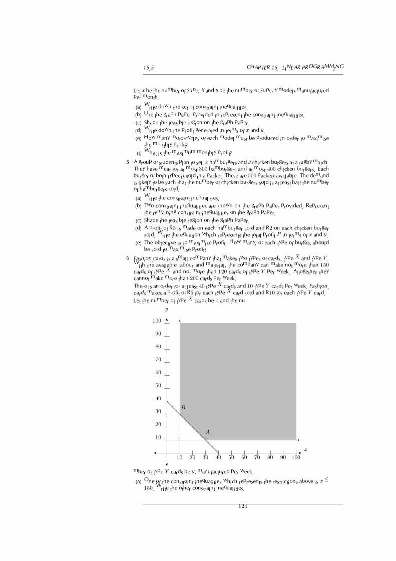
15.5 CHAPTER 15. LINEAR PROGRAMMING
Let x be the number of Super X and y be the number of Super Ymodels manufactured
per month.
(a) Write down the set of constraint inequalities.
(b) Use the graph paper provided to represent the constraint inequalities.
(c) Shade the feasible region on the graph paper.
(d) Write down the profit generated in terms of x and y.
(e) How many motorcycles of each model must be produced in order to maximise
the monthly profit?
(f) What is the maximum monthly profit?
5. A group of students plan to sell x hamburgers and y chicken burgers at a rugby match.They have meat for at most 300 hamburgers and at most 400 chicken burgers. Each
burger of both types is sold in a packet. There are 500 packets available. The demandis likely to be such that the number of chicken burgers sold is at least half the number
of hamburgers sold.
(a) Write the constraint inequalities.
(b) Two constraint inequalities are shown on the graph paper provided. Represent
the remaining constraint inequalities on the graph paper.
(c) Shade the feasible region on the graph paper.
(d) A profit of R3 is made on each hamburger sold and R2 on each chicken burger
sold. Write the equation which represents the total profit P in terms of x and y.
(e) The objective is to maximise profit. How many, of each type of burger, should
be sold to maximise profit?
6. Fashion-cards is a small company that makes two types of cards, type X and type Y .
With the available labour and material, the company can make not more than 150cards of type X and not more than 120 cards of type Y per week. Altogether they
cannot make more than 200 cards per week.
There is an order for at least 40 typeX cards and 10 type Y cards per week. Fashion-
cards makes a profit of R5 for each type X card sold and R10 for each type Y card.
Let the number of type X cards be x and the nu
10
20
30
40
50
60
70
80
90
100
10 20 30 40 50 60 70 80 90 100
x
y
A
B
mber of type Y cards be y, manufactured per week.
(a) One of the constraint inequalities which represents the restrictions above is x ≤150. Write the other constraint inequalities.
124

CHAPTER 15. LINEAR PROGRAMMING 15.5
(b) Represent the constraints graphically and shade the feasible region.
(c) Write the equation that represents the profit P (the objective function), in terms
of x and y.
(d) Calculate the maximum weekly profit.
7. To meet the requirements of a specialised diet a meal is prepared by mixing two
types of cereal, Vuka and Molo. The mixture must contain x packets of Vuka cereal
and y packets of Molo cereal. The meal requires at least 15 g of protein and at least
72 g of carbohydrates. Each packet of Vuka cereal contains 4 g of protein and 16g of carbohydrates. Each packet of Molo cereal contains 3 g of protein and 24 g of
carbohydrates. There are at most 5 packets of cereal available. The feasible region is
shaded on the attached graph paper.
(a) Write down the constraint inequalities.
(b) If Vuka cereal costs R6 per packet and Molo cereal also costs R6 per packet, usethe graph to determine how many packets of each cereal must be used for the
mixture to satisfy the above constraints in each of the following cases:
i. The total cost is a minimum.
ii. The total cost is a maximum (give all possibilities).
0 1 2 3 4 5 60
1
2
3
4
5
6
0
1
2
3
4
5
6
0 1 2 3 4 5 6Number of packets of Vuka
NumberofpacketsofMolo
8. A bicycle manufacturer makes two different models of bicycles, namely mountain
bikes and speed bikes. The bicycle manufacturer works under the following con-
straints:
No more than 5 mountain bicycles can be assembled daily.
No more than 3 speed bicycles can be assembled daily.It takes one man to assemble a mountain bicycle, two men to assemble a speed bi-
cycle and there are 8 men working at the bicycle manufacturer.Let x represent the number of mountain bicycles and let y represent the number of
speed bicycles.
(a) Determine algebraically the constraints that apply to this problem.
(b) Represent the constraints graphically on the graph paper.
(c) By means of shading, clearly indicate the feasible region on the graph.
(d) The profit on a mountain bicycle is R200 and the profit on a speed bicycle is
R600. Write down an expression to represent the profit on the bicycles.
(e) Determine the number of each model bicycle that would maximise the profit to
the manufacturer.
125

15.5 CHAPTER 15. LINEAR PROGRAMMING
More practice video solutions or help at www.everythingmaths.co.za
(1.) 012k (2.) 012m (3.) 012n (4.) 012p (5.) 012q (6.) 012r
(7.) 012s (8.) 012t
126

Geometry 16
16.1 Introduction EMBCF
Geometry is a good subject for learning not just about the mathematics of two and three-dimensional
shapes, but also about how we construct mathematical arguments. In this chapter you will learn how
to prove geometric theorems and discover some of the properties of shapes through small logical steps.
See introductory video: VMfqd at www.everythingmaths.co.za
16.2 Right Pyramids, Right Conesand Spheres
EMBCG
A pyramid is a geometric solid that has a polygon base and the base is joined to a point, called the
apex. Two examples of pyramids are shown in the left-most and centre figures in Figure 16.1. The
right-most figure has an apex which is joined to a circular base and this type of geometric solid is
called a cone. Cones are similar to pyramids except that their bases are circles instead of polygons.
Figure 16.1: Examples of a square pyramid, a triangular pyramid and a cone.
Surface Area of a Pyramid
The surface area of a pyramid is calculated by adding the area of each face together.
Example 1: Surface Area
QUESTION
If a cone has a height of h and a base of radius r, show that the surface area is πr2 +πr
√r2 + h2.
127

16.2 CHAPTER 16. GEOMETRY
SOLUTION
Step 1 : Draw a picture
r
h
r
ha
Step 2 : Identify the faces that make up the cone
The cone has two faces: the base and the walls. The base is a circle of radius rand the walls can be opened out to a sector of a circle.
a
2πr = circumference
This curved surface can be cut into many thin triangles with height close to a (a iscalled the slant height). The area of these triangles will add up to 1
2×base×height(of
a small triangle) which is 12× 2πr × a = πra
Step 3 : Calculate aa can be calculated by using the Theorem of Pythagoras. Therefore:
a =�
r2 + h2
Step 4 : Calculate the area of the circular base
Ab = πr2
Step 5 : Calculate the area of the curved walls
Aw = πra
= πr�
r2 + h2
Step 6 : Calculate surface area A
A = Ab +Aw
= πr2 + πr�
r2 + h2
128

CHAPTER 16. GEOMETRY 16.2
Volume of a Pyramid: The volume of a pyramid is found by:
V =1
3A . h
where A is the area of the base and h is the perpendicular height.
A cone is like a pyramid, so the volume of a cone is given by:
V =1
3πr2h.
A square pyramid has volume
V =1
3a2h
where a is the side length of the square base.
See video: VMfqj at www.everythingmaths.co.za
Example 2: Volume of a Pyramid
QUESTION
What is the volume of a square pyramid, 3 cm high with a side length of 2 cm?
SOLUTION
Step 1 : Determine the correct formula
The volume of a pyramid is
V =1
3A . h,
where A is the area of the base and h is the height of the pyramid. For a square
base this means
V =1
3a . a . h
where a is the length of the side of the square base.
2 cm2 cm
3 cm
�
129

16.2 CHAPTER 16. GEOMETRY
Step 2 : Substitute the given values
=1
3. 2 . 2 . 3
=1
3. 12
= 4 cm3
We accept the following formulae for volume and surface area of a sphere (ball).
Surface area = 4πr2
Volume =4
3πr3
Exercise 16 - 1
1. Calculate the volumes and surface areas of the following solids: (Hint for (e): find the perpen-
dicular height using Pythagoras).
�
�
�
�
4
6
7
14
3
513
24
24
a) b) c) d) e)
a spherea conea hemisphere
a hemisphere on
top of a cone
a pyramid with
a square base
2. Water covers approximately 71% of the Earth’s surface. Taking the radius of the Earth to be 6378km, what is the total area of land (area not covered by water)?
130

CHAPTER 16. GEOMETRY 16.3
3.
A triangular pyramid is placed on top of a triangular
prism. The prism has an equilateral triangle of side
length 20 cm as a base, and has a height of 42 cm.The pyramid has a height of 12 cm.
(a) Find the total volume of the object.
(b) Find the area of each face of the pyramid.
(c) Find the total surface area of the object.
More practice video solutions or help at www.everythingmaths.co.za
(1.) 012u (2.) 012v (3.) 012w
16.3 Similarity of Polygons EMBCH
In order for two polygons to be similar the following must be true:
1. All corresponding angles must be congruent.
2. All corresponding sides must be in the same proportion to each other. Refer to the picture below:
this means that the ratio of side AE on the large polygon to the side PT on the small polygon
must be the same as the ratio of side AB to side PQ, BC/QR etc. for all the sides.
B
D C
A
ET
S R
Q
P
If
1. A = P ; B = Q; C = R; D = S;E = Tand
2. ABPQ
= BCQR
= CDRS
= DEST
= EATP
then the polygons ABCDE and
PQRST are similar.
131

16.3 CHAPTER 16. GEOMETRY
Example 3: Similarity of Polygons
QUESTION
Polygons PQTU and PRSU are sim-
ilar. Find the value of x. P
T
S
Q
R
U
x
3−x
31
Polygons PQTU and PRSU are sim-
ilar. Find the value of x. P
T
S
Q
R
U
x
3−x
31
SOLUTION
Step 1 : Identify corresponding sides
Since the polygons are similar,
PQ
PR=
TU
SU
∴x
x+ (3− x)=
3
4
∴x
3=
3
4
∴ x =9
4
132

CHAPTER 16. GEOMETRY 16.4
16.4 Triangle Geometry EMBCI
Proportion EMBCJ
Two line segments are divided in the same proportion if the ratios between their parts are equal.
AB
BC=
x
y=
kx
ky=
DE
EF
∴ the line segments are in the same proportion
A
B
C
D
E
F
x
y
kx
ky
If the line segments are proportional, the following also hold:
1. CBAC
= FEDF
2. AC .FE = CB .DF
3. ABBC
= DEFE
and BCAB
= FEDE
4. ABAC
= DEDF
and ACAB
= DFDE
Proportionality of triangles
Triangles with equal heights have areas which are in the same proportion to each other as the bases of
the triangles.
h1 = h2
∴area �ABC
area �DEF=
12BC × h1
12EF × h2
=BC
EF
A
B C
D
E F
h1
h2
133

16.4 CHAPTER 16. GEOMETRY
• A special case of this happens when the bases of the triangles are equal:
Triangles with equal bases between the same parallel lines have the same area.
area �ABC =1
2. h . BC = area �DBC
A
B C
D
h
• Triangles on the same side of the same base, with equal areas, lie between parallel lines.
If area �ABC = area �BDC
then AD � BC
A
B C
D
Theorem 1. Proportion Theorem: A line drawn parallel to one side of a triangle divides the other two
sides proportionally.
AAA
C BBB
CC
D
D
D
E
E
E
h1
h2
Given:�ABC with line DE � BC
R.T.P.:
AD
DB=
AE
EC
Proof: Draw h1 from E perpendicular to AD, and h2 from D perpendicular to AE.
134

CHAPTER 16. GEOMETRY 16.4
Draw BE and CD.
area �ADE
area �BDE=
12AD . h1
12DB . h1
=AD
DB
area �ADE
area �CED=
12AE . h2
12EC . h2
=AE
EC
but area �BDE = area �CED (equal base and height)
∴area �ADE
area �BDE=
area �ADE
area �CED
∴AD
DB=
AE
EC∴ DE divides AB and AC proportionally.
Similarly,
AD
AB=
AE
ACAB
BD=
AC
CE
Following from Theorem 1, we can prove the midpoint theorem.
Theorem 2. Midpoint Theorem: A line joining the midpoints of two sides of a triangle is parallel to
the third side and equal to half the length of the third side.
Proof:
This is a special case of the Proportionality Theorem (Theorem 1).
If AB = BD and AC = AE,
and
AD = AB +BD = 2ABAE = AC + CB = 2ACthen DE � BC and BC = 2DE.
A
B C
D E
Theorem 3. Similarity Theorem 1: Equiangular triangles have their sides in proportion and are there-
fore similar.
A
F
H
B C
D
E
G
�
�
Given:�ABC and �DEF with A = D; B = E; C = F
R.T.P.:AB
DE=
AC
DF
Construct: G on AB, so that AG = DEH on AC, so that AH = DF
135

16.4 CHAPTER 16. GEOMETRY
Proof: In �’s AGH and DEF
AG = DE;AH = DF (constant)
A = D (given)
∴ �AGH ≡ �DEF (SAS)
∴ AGH = E = B
∴ GH � BC (corresponding ∠’s equal)
∴AG
AB=
AH
AC(proportion theorem)
∴DE
AB=
DF
AC(AG = DE; AH = DF )
∴ �ABC ||| �DEFTip
||| means “is similar to”Theorem 4. Similarity Theorem 2: Triangles with sides in proportion are equiangular and therefore
similar.
A
CB
D E
h1
h2
Given:�ABC with line DE such thatAD
DB=
AE
EC
R.T.P.: DE � BC; �ADE ||| �ABC
Proof:
Draw h1 from E perpendicular to AD, and h2 from D perpendicular to AE.
Draw BE and CD.
area �ADE
area �BDE=
12AD . h1
12DB . h1
=AD
DB
area �ADE
area �CED=
12AE . h2
12EC . h2
=AE
EC
butAD
DB=
AE
EC(given)
∴area �ADE
area �BDE=
area �ADE
area �CED
∴ area �BDE = area �CED
∴ DE � BC (same side of equal base DE, same area)
∴ ADE = ABC (corresponding ∠’s)
and AED = ACB
∴ �ADE and �ABC are equiangular
∴ �ADE ||| �ABC (AAA)
Theorem 5. Pythagoras’ Theorem: The square on the hypotenuse of a right angled triangle is equal to
the sum of the squares on the other two sides.
136

CHAPTER 16. GEOMETRY 16.4
Given:�ABC with A = 90◦
1
2
A
B CD
2
1
R.T.P.: BC2 = AB2 +AC2
Proof:
Let C = x
∴ DAC = 90◦ − x (∠’s of a � )
∴ DAB = x
ABD = 90◦ − x (∠’s of a � )
BDA = CDA = A = 90◦
∴ �ABD|||�CBA and �CAD|||�CBA (AAA)
∴AB
CB=
BD
BA=
�
AD
CA
�
andCA
CB=
CD
CA=
�
AD
BA
�
∴ AB2 = CB ×BD and AC2 = CB × CD
∴ AB2 +AC2 = CB(BD + CD)
= CB(CB)
= CB2
i.e. BC2 = AB2 +AC2
137

16.4 CHAPTER 16. GEOMETRY
Example 4: Triangle Geometry 1
QUESTION
In �GHI, GH � LJ ; GJ � LK and JKKI
= 53. Determine HJ
KI.
SOLUTION
G
H
I
J
K
L
Step 1 : Identify similar triangles
LIJ = GIH
JLI = HGI (Corresponding ∠’s)
∴ �LIJ ||| �GIH (Equiangular �’s)
LIK = GIJ
KLI = JGI (Corresponding ∠’s)
∴ �LIK ||| �GIJ (Equiangular �’s)
Step 2 : Use proportional sides
HJ
JI=
GL
LI(�LIJ ||| �GIH)
andGL
LI=
JK
KI(�LIK ||| �GIJ)
=5
3
∴HJ
JI=5
3
Step 3 : Rearrange to find the required ratio
HJ
KI=
HJ
JI× JI
KI
138

CHAPTER 16. GEOMETRY 16.4
We need to calculate JIKI
: We were given JKKI
= 53So rearranging, we have
JK = 53KI And:
JI = JK +KI
=5
3KI +KI
=8
3KI
JI
KI=
8
3
Using this relation:
=5
3× 8
3
=40
9
Example 5: Triangle Geometry 2
QUESTION
PQRS is a trapezium, with PQ � RS.Prove that PT . TR = ST . TQ.
1
21
1 12 2
2
T
P Q
R S
SOLUTION
Step 4 : Identify similar triangles
P1 = S1 (alternate ∠’s)
Q1 = R1 (alternate ∠’s)
∴ �PTQ ||| �STR (equiangular �’s)
Step 5 : Use proportional sides
PT
TQ=
ST
TR(�PTQ|||�STR)
∴ PT . TR = ST . TQ
139

16.4 CHAPTER 16. GEOMETRY
Exercise 16 - 2
1. Calculate SV
� �
S
T
U
V10
W
20
35
2. CBYB
= 32. Find DS
SB.
X
Y
Z
A
BC
D
S
3. Given the following figure with the following lengths, find AE, EC and BE.
BC = 15 cm, AB = 4 cm, CD = 18 cm, and ED = 9 cm.
A
B
C
D
E
4. Using the following figure and lengths, find IJ and KJ .HI = 26 m, KL = 13 m, JL = 9 m and HJ = 32 m.
H
I
JK
L
140
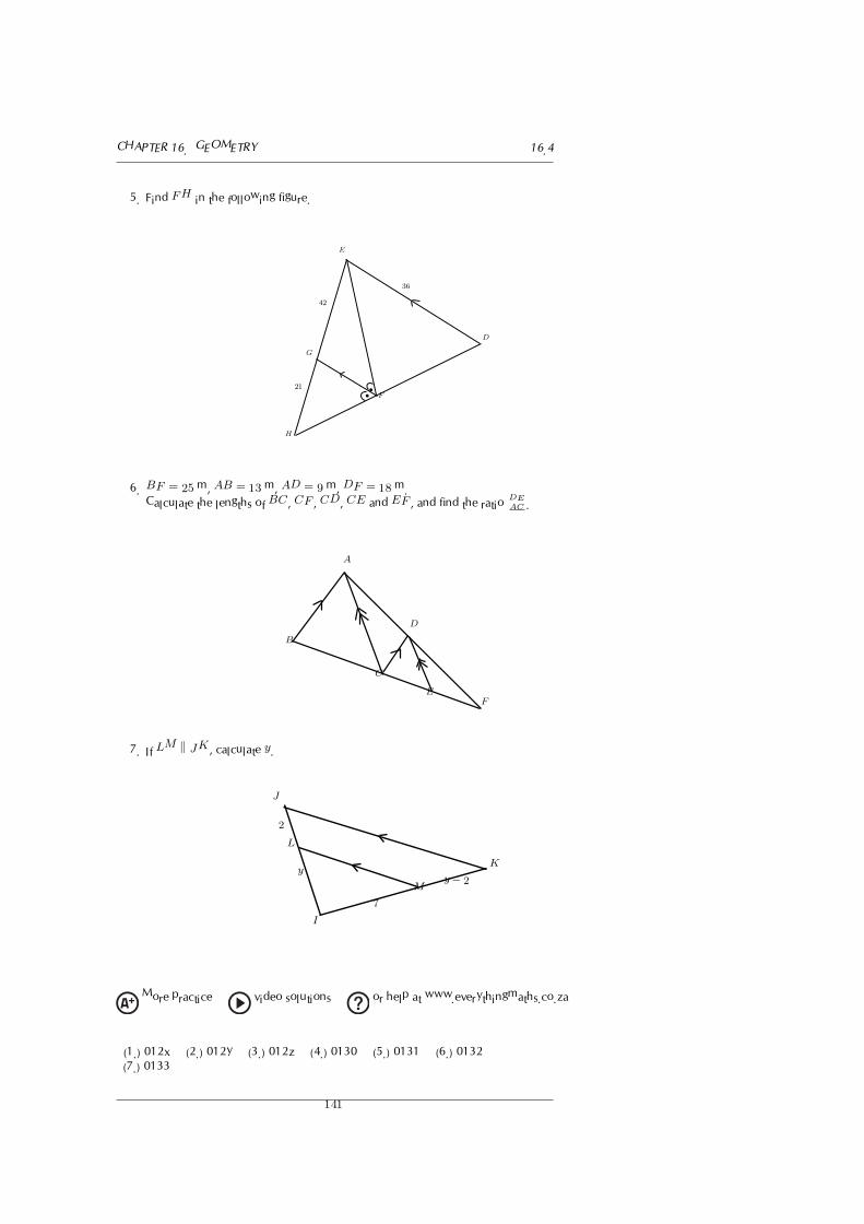
CHAPTER 16. GEOMETRY 16.4
5. Find FH in the following figure.
��
E
D
F
G
H
42
21
36
6. BF = 25 m, AB = 13 m, AD = 9 m, DF = 18 m.Calculate the lengths of BC, CF , CD, CE and EF , and find the ratio DE
AC.
A
B
C
D
EF
7. If LM � JK, calculate y.
I
J
K
L
M
yy − 2
2
7
More practice video solutions or help at www.everythingmaths.co.za
(1.) 012x (2.) 012y (3.) 012z (4.) 0130 (5.) 0131 (6.) 0132
(7.) 0133
141

16.5 CHAPTER 16. GEOMETRY
16.5 Co-ordinate Geometry EMBCK
Equation of a Line Between Two Points EMBCL
See video: VMftf at www.everythingmaths.co.za
There are many different methods of specifying the requirements for determining the equation of a
straight line. One option is to find the equation of a straight line, when two points are given.
Assume that the two points are (x1; y1) and (x2; y2), and we know that the general form of the equation
for a straight line is:
y = mx+ c (16.1)
So, to determine the equation of the line passing through our two points, we need to determine values
for m (the gradient of the line) and c (the y-intercept of the line). The resulting equation is
y − y1 = m(x− x1) (16.2)
where (x1; y1) are the co-ordinates of either given point.
Tip
If you are asked to cal-culate the equation of aline passing through twopoints, use:
m =y2 − y1
x2 − x1
to calculate m and thenuse:
y − y1 = m(x− x1)
to determine the equa-tion.
Extension: Finding the second equation for a straight line
This is an example of a set of simultaneous equations, because we can write:
y1 = mx1 + c (16.3)
y2 = mx2 + c (16.4)
We now have two equations, with two unknowns, m and c.
Subtract (16.3) from (16.4) y2 − y1 = mx2 −mx1 (16.5)
∴ m =y2 − y1x2 − x1
(16.6)
Re-arrange (16.3) to obtain c y1 = mx1 + c (16.7)
c = y1 −mx1 (16.8)
Now, to make things a bit easier to remember, substitute (16.7) into (16.1):
y = mx+ c (16.9)
= mx+ (y1 −mx1) (16.10)
which can be re-arranged to: y − y1 = m(x− x1) (16.11)
For example, the equation of the straight line passing through (−1; 1) and (2; 2) is given by first calcu-
142

CHAPTER 16. GEOMETRY 16.5
lating m
m =y2 − y1x2 − x1
=2− 1
2− (−1)
=1
3
and then substituting this value into
y − y1 = m(x− x1)
to obtain
y − y1 =1
3(x− x1).
Then substitute (−1; 1) to obtain
y − (1) =1
3(x− (−1))
y − 1 =1
3x+
1
3
y =1
3x+
1
3+ 1
y =1
3x+
4
3
So, y = 13x+ 4
3passes through (−1; 1) and (2; 2).
1
2
3
1 2 3−1−2−3
�
�
(−1; 1)
(2; 2)
y = 13x+ 4
3
x
y
Figure 16.2: The equation of the line passing through (−1; 1) and (2; 2) is y = 13x+ 4
3.
Example 6: Equation of Straight Line
QUESTION
Find the equation of the straight line passing through (−3; 2) and (5; 8).
143

16.5 CHAPTER 16. GEOMETRY
SOLUTION
Step 1 : Label the points
(x1; y1) = (−3; 2)(x2; y2) = (5; 8)
Step 2 : Calculate the gradient
m =y2 − y1x2 − x1
=8− 2
5− (−3)
=6
5 + 3
=6
8
=3
4
Step 3 : Determine the equation of the line
y − y1 = m(x− x1)
y − (2) =3
4(x− (−3))
y =3
4(x+ 3) + 2
=3
4x+
3
4. 3 + 2
=3
4x+
9
4+8
4
=3
4x+
17
4
Step 4 : Write the final answer
The equation of the straight line that passes through (−3; 2) and (5; 8) is y =34x+ 17
4.
Equation of a Line Through One Point andParallel or Perpendicular to Another Line
EMBCM
Another method of determining the equation of a straight-line is to be given one point, (x1; y1), and tobe told that the line is parallel or perpendicular to another line. If the equation of the unknown line is
144

CHAPTER 16. GEOMETRY 16.5
y = mx+ c and the equation of the second line is y = m0x+ c0, then we know the following:
If the lines are parallel, then m = m0 (16.12)
If the lines are perpendicular, then m×m0 = −1 (16.13)
Once we have determined a value for m, we can then use the given point together with:
y − y1 = m(x− x1)
to determine the equation of the line.
For example, find the equation of the line that is parallel to y = 2x−1 and that passes through (−1; 1).First we determine m, the slope of the line we are trying to find. Since the line we are looking for is
parallel to y = 2x− 1,m = 2
The equation is found by substituting m and (−1; 1) into:
y − y1 = m(x− x1)
y − 1 = 2(x− (−1)y − 1 = 2(x+ 1)
y − 1 = 2x+ 2
y = 2x+ 2 + 1
y = 2x+ 3
1
2
3
−1
−2
1 2 3−1−2−3
�(−1; 1) y = 2x− 1
y = 2x+ 3
x
y
Figure 16.3: The equation of the line passing through (−1; 1) and parallel to y = 2x−1 is y = 2x+3. Itcan be seen that the lines are parallel to each other. You can test this by using your ruler and measuring
the perpendicular distance between the lines at different points.
Inclination of a Line EMBCN
In Figure 16.4(a), we see that the line makes an angle θ with the x-axis. This angle is known as the
inclination of the line and it is sometimes interesting to know what the value of θ is.
145

16.5 CHAPTER 16. GEOMETRY
1
2
3
1 2 3
θ
Δy
Δx
x
y
1
2
3
1 2 3 4
f(x) = 4x− 4
g(x) = 2x− 2
θg θfx
y
(a) (b)
Figure 16.4: (a) A line makes an angle θ with the x-axis. (b) The angle is dependent on the gradient. Ifthe gradient of f is mf and the gradient of g is mg then mf > mg and θf > θg.
Firstly, we note that if the gradient changes, then the value of θ changes (Figure 16.4(b)), so we suspectthat the inclination of a line is related to the gradient. We know that the gradient is a ratio of a change
in the y-direction to a change in the x-direction.
m =Δy
Δx
But, in Figure 16.4(a) we see that
tan θ =Δy
Δx∴ m = tan θ
For example, to find the inclination of the line y = x, we know m = 1
∴ tan θ = 1
∴ θ = 45◦
Exercise 16 - 3
1. Find the equations of the following lines
(a) through points (−1; 3) and (1; 4)(b) through points (7;−3) and (0; 4)(c) parallel to y = 1
2x+ 3 passing through (−1; 3)
(d) perpendicular to y = − 12x+ 3 passing through (−1; 2)
(e) perpendicular to 2y + x = 6 passing through the origin
2. Find the inclination of the following lines
(a) y = 2x− 3(b) y = 1
3x− 7
(c) 4y = 3x+ 8
(d) y = − 23x+ 3 (Hint: if m is negative θ must be in the second quadrant)
(e) 3y + x− 3 = 0
3. Show that the line y = k for any constant k is parallel to the x-axis. (Hint: Show that the
inclination of this line is 0◦.)
146

CHAPTER 16. GEOMETRY 16.6
4. Show that the line x = k for any constant k is parallel to the y-axis. (Hint: Show that the
inclination of this line is 90◦.)
More practice video solutions or help at www.everythingmaths.co.za
(1.) 0134 (2.) 0135 (3.) 0136 (4.) 0137
16.6 Transformations EMBCO
Rotation of a Point EMBCP
When something is moved around a fixed point, we say that it is rotated about the point. What happens
to the coordinates of a point that is rotated by 90◦ or 180◦ around the origin?
Activity: Rotation of a Point by 90◦
Complete the table, by filling in the coordinates of the points shown in the figure.
Point x-coordinate y-coordinate
A
B
C
D
E
F
G
H
�
���
�
� ��
A
BC
D
E
FG
H
What do you notice about the x-coordinates? What do you notice about the y-coordinates?What would happen to the coordinates of point A, if it was rotated to the position of point C?
What about if point B rotated to the position of D?
Activity: Rotation of a Point by 180◦
Complete the table, by filling in the coordinates of the points shown in the figure.
147

16.6 CHAPTER 16. GEOMETRY
Point x-coordinate y-coordinate
A
B
C
D
E
F
G
H
�
���
�
� ��
A
BC
D
E
FG
H
What do you notice about the x-coordinates? What do you notice about the y-coordinates?What would happen to the coordinates of point A, if it was rotated to the position of point E?
What about point F rotated to the position of B?
From these activities you should have come to the following conclusions:
• 90◦ clockwise rotation:The image of a point P (x; y) rotated clockwise
through 90◦ around the origin is P �(y;−x).We write the rotation as (x; y)→ (y;−x).
x
y
P (x; y)
P �(y;−x)
�
�
• 90◦ anticlockwise rotation:The image of a point P (x; y) rotated anticlockwisethrough 90◦ around the origin is P �(−y;x).We write the rotation as (x; y)→ (−y;x).
x
y
P (x; y)
P ��(−y; x)
�
�
• 180◦ rotation:The image of a point P (x; y) rotated through 180◦
around the origin is P �(−x;−y).We write the rotation as (x; y)→ (−x;−y).
x
y
P (x; y)
P ���(−x;−y)
�
�
Exercise 16 - 4
1. For each of the following rotations about the origin:
(i) Write down the rule.
(ii) Draw a diagram showing the direction of rotation.
(a) OA is rotated to OA� with A(4; 2) and A�(−2; 4)(b) OB is rotated to OB� with B(−2; 5) and B�(5; 2)
148

CHAPTER 16. GEOMETRY 16.6
(c) OC is rotated to OC � with C(−1;−4) and C �(1; 4)
2. Copy ΔXY Z onto squared paper. The co-ordinates are given on the picture.
(a) Rotate ΔXY Z anti-clockwise through an angle of 90◦ about the origin to give ΔX �Y �Z �.
Give the co-ordinates of X �, Y � and Z �.
(b) Rotate ΔXY Z through 180◦ about the origin to give ΔX ��Y ��Z ��. Give the co-ordinates of
X ��, Y ��and Z ��.
X(4; 4)
Y (−1;−4)
Z(−4;−1)
More practice video solutions or help at www.everythingmaths.co.za
(1.) 0138 (2.) 0139
Enlargement of a Polygon EMBCQ
When something is made larger, we say that it is enlarged. What happens to the coordinates of a
polygon that is enlarged by a factor k?
Activity: Enlargement of a Polygon
Complete the table, by filling in the coordinates of the points shown in the figure. Assume
each small square on the plot is 1 unit.
149

16.6 CHAPTER 16. GEOMETRY
Point x-coordinate y-coordinate
A
B
C
D
E
F
G
H
EF
G H
AB
C D
��
� �
�
��
�
What do you notice about the x-coordinates? What do you notice about the y-coordinates?What would happen to the coordinates of point A, if the square ABCD was enlarged by a
factor of 2?
Activity: Enlargement of a Polygon
H
I
JK
H�
I�
J �K�
0 1 2 3 4 5 6 7 8 9
0
1
2
3
4
5
6
7
In the figure quadrilateral HIJK has been enlarged by a factor of 2 through the origin to be-
come H �I �J �K�. Complete the following table using the information in the figure.
Co-ordinate Co-ordinate’ Length Length’
H = ( ; ) H � = ( ; ) OH = OH � =
I = ( ; ) I � = ( ; ) OI = OI � =J = ( ; ) J � = ( ; ) OJ = OJ � =
K = ( ; ) K� = ( ; ) OK = OK� =
What conclusions can you draw about
1. the co-ordinates
2. the lengths when we enlarge by a factor of 2?
We conclude as follows:
Let the vertices of a triangle have co-ordinates S(x1; y1), T (x2; y2), U(x3; y3). �S�T �U � is an enlarge-
ment through the origin of �STU by a factor of c (c > 0).
• �STU is a reduction of �S�T �U � by a factor of c.
• �S�T �U � can alternatively be seen as an reduction through the origin of �STU by a factor of1c. (Note that a reduction by 1
cis the same as an enlargement by c).
• The vertices of �S�T �U � are S�(cx1; cy1), T�(cx2,cy2), U
�(cx3,cy3).
150

CHAPTER 16. GEOMETRY 16.6
• The distances from the origin are OS� = (c . OS), OT � = (c . OT ) and OU � = (c . OU).
S
T
U
S�
U �
T �
0 1 2 3 4 5 6 7 8 9 10 11
0
1
2
3
4
5
6
7
8
9
Chapter 16 End of Chapter Exercises
1. Copy polygon STUV onto squared paper and then answer the following questions.
-3 -2 -1 0 1 2 3 4 5
-3
-2
-1
0
1
2
3
S
T
U
V
(a) What are the co-ordinates of polygon STUV ?
(b) Enlarge the polygon through the origin by a constant factor of c = 2. Draw this
on the same grid. Label it S�T �U �V �.
151

16.6 CHAPTER 16. GEOMETRY
(c) What are the co-ordinates of the vertices of S�T �U �V �?
2. �ABC is an enlargement of �A�B�C � by a constant factor of k through the origin.
-5 -4 -3 -2 -1 0 1 2 3 4 5
-5
-4
-3
-2
-1
0
1
2
3
4
5
C
A
BA�
B�
C�
(a) What are the co-ordinates of the vertices of �ABC and �A�B�C �?
(b) Giving reasons, calculate the value of k.
(c) If the area of �ABC is m times the area of �A�B�C �, what is m?
3. Examine the polygon below.
-2 -1 0 1 2 3 4 5
-2
-1
0
1
2
3
4
5
M
N
Q
P
(a) What are the co-ordinates of the vertices of polygon MNPQ?
(b) Enlarge the polygon through the origin by using a constant factor of c = 3,obtaining polygon M �N �P �Q�. Draw this on the same set of axes.
152

CHAPTER 16. GEOMETRY 16.6
(c) What are the co-ordinates of the new vertices?
(d) Now draw M ��N ��P ��Q�� which is an anticlockwise rotation of MNPQ by 90◦
around the origin.
(e) Find the inclination of OM ��.
More practice video solutions or help at www.everythingmaths.co.za
(1.) 01zi (2.) 01zj (3.) 01zk
153

Trigonometry 17
17.1 Introduction EMBCR
Building on Grade 10 Trigonometry, we will look at more general forms of the the basic trigonometric
functions next. We will use graphs and algebra to analyse the properties of these functions. We will
also see that different trigonometric functions are closely related through a number of mathematical
identities.
See introductory video: VMfva at www.everythingmaths.co.za
17.2 Graphs of TrigonometricFunctions
EMBCS
Functions of the Form y = sin(kθ) EMBCT
In the equation, y = sin(kθ), k is a constant and has different effects on the graph of the function.
The general shape of the graph of functions of this form is shown in Figure 17.1 for the function
f(θ) = sin(2θ).
1
−190 180 270−90−180−270
Figure 17.1: Graph of f(θ) = sin(2θ) (solid line) and the graph of g(θ) = sin(θ) (dotted line).
Exercise 17 - 1
On the same set of axes, plot the following graphs:
1. a(θ) = sin 0,5θ
2. b(θ) = sin 1θ
3. c(θ) = sin 1,5θ
154

CHAPTER 17. TRIGONOMETRY 17.2
4. d(θ) = sin 2θ
5. e(θ) = sin 2,5θ
Use your results to deduce the effect of k.
More practice video solutions or help at www.everythingmaths.co.za
(1.) 013c
You should have found that the value of k affects the period or frequency of the graph. Notice that in
the case of the sine graph, the period (length of one wave) is given by 360◦
k.
These different properties are summarised in Table 17.1.
Table 17.1: Table summarising general shapes and positions of graphs of functions of the form
y = sin(kx). The curve y = sin(x) is shown as a dotted line.
k > 0 k < 0
Domain and Range
For f(θ) = sin(kθ), the domain is {θ : θ ∈ R} because there is no value of θ ∈ R for which f(θ) isundefined.
The range of f(θ) = sin(kθ) is {f(θ) : f(θ) ∈ [−1; 1]}.
Intercepts
For functions of the form, y = sin(kθ), the details of calculating the intercepts with the y axis are
given.
There are many x-intercepts.
The y-intercept is calculated by setting θ = 0:
y = sin(kθ)
yint = sin(0)
= 0
155

17.2 CHAPTER 17. TRIGONOMETRY
Functions of the Form y = cos(kθ) EMBCU
In the equation, y = cos(kθ), k is a constant and has different effects on the graph of the function.
The general shape of the graph of functions of this form is shown in Figure 17.2 for the function
f(θ) = cos(2θ).
1
-1
45 90 135 180 225 270 315-45-90-135-180-225-270-315
Figure 17.2: Graph of f(θ) = cos(2θ) (solid line) and the graph of g(θ) = cos(θ) (dotted line).
Exercise 17 - 2
On the same set of axes, plot the following graphs:
1. a(θ) = cos 0,5θ
2. b(θ) = cos 1θ
3. c(θ) = cos 1,5θ
4. d(θ) = cos 2θ
5. e(θ) = cos 2,5θ
Use your results to deduce the effect of k.
More practice video solutions or help at www.everythingmaths.co.za
(1.) 013h
You should have found that the value of k affects the period or frequency of the graph. The period of
the cosine graph is given by 360◦
k.
These different properties are summarised in Table 17.2.
Domain and Range
For f(θ) = cos(kθ), the domain is {θ : θ ∈ R} because there is no value of θ ∈ R for which f(θ) isundefined.
The range of f(θ) = cos(kθ) is {f(θ) : f(θ) ∈ [−1; 1]}.
156

CHAPTER 17. TRIGONOMETRY 17.2
Table 17.2: Table summarising general shapes and positions of graphs of functions of the form
y = cos(kx). The curve y = cos(x) is plotted with a dotted line.
k > 0 k < 0
Intercepts
For functions of the form, y = cos(kθ), the details of calculating the intercepts with the y axis are
given.
The y-intercept is calculated as follows:
y = cos(kθ)
yint = cos(0)
= 1
Functions of the Form y = tan(kθ) EMBCV
In the equation, y = tan(kθ), k is a constant and has different effects on the graph of the function.
The general shape of the graph of functions of this form is shown in Figure 17.3 for the function
f(θ) = tan(2θ).
5
−590 180 270 360−90−180−270−360
Figure 17.3: The graph of f(θ) = tan(2θ) (solid line) and the graph of g(θ) = tan(θ) (dotted line).
The asymptotes are shown as dashed lines.
Exercise 17 - 3
On the same set of axes, plot the following graphs:
1. a(θ) = tan 0,5θ
157

17.2 CHAPTER 17. TRIGONOMETRY
2. b(θ) = tan 1θ
3. c(θ) = tan 1,5θ
4. d(θ) = tan 2θ
5. e(θ) = tan 2,5θ
Use your results to deduce the effect of k.
More practice video solutions or help at www.everythingmaths.co.za
(1.) 013n
You should have found that, once again, the value of k affects the periodicity (i.e. frequency) of the
graph. As k increases, the graph is more tightly packed. As k decreases, the graph is more spread out.
The period of the tan graph is given by 180◦
k.
These different properties are summarised in Table 17.3.
Table 17.3: Table summarising general shapes and positions of graphs of functions of the form
y = tan(kθ).
k > 0 k < 0
Domain and Range
For f(θ) = tan(kθ), the domain of one branch is {θ : θ ∈ (− 90◦
k; 90
◦
k)} because the function is
undefined for θ = − 90◦
kand θ = 90◦
k.
The range of f(θ) = tan(kθ) is {f(θ) : f(θ) ∈ (−∞;∞)}.
Intercepts
For functions of the form, y = tan(kθ), the details of calculating the intercepts with the x and y axis
are given.
There are many x-intercepts; each one is halfway between the asymptotes.
The y-intercept is calculated as follows:
y = tan(kθ)
yint = tan(0)
= 0
Asymptotes
The graph of tan kθ has asymptotes because as kθ approaches 90◦, tan kθ approaches infinity. In otherwords, there is no defined value of the function at the asymptote values.
158

CHAPTER 17. TRIGONOMETRY 17.2
Functions of the Form y = sin(θ + p) EMBCW
In the equation, y = sin(θ + p), p is a constant and has different effects on the graph of the function.
The general shape of the graph of functions of this form is shown in Figure 17.4 for the function
f(θ) = sin(θ + 30◦).
1
-1
30 60 90 120 150 180 210 240 270 300 330-30-60-90-120-150-180-210-240-270-300-330
Figure 17.4: Graph of f(θ) = sin(θ + 30◦) (solid line) and the graph of g(θ) = sin(θ) (dotted line).
Exercise 17 - 4
On the same set of axes, plot the following graphs:
1. a(θ) = sin(θ − 90◦)
2. b(θ) = sin(θ − 60◦)
3. c(θ) = sin θ
4. d(θ) = sin(θ + 90◦)
5. e(θ) = sin(θ + 180◦)
Use your results to deduce the effect of p.
More practice video solutions or help at www.everythingmaths.co.za
(1.) 013t
You should have found that the value of p affects the position of the graph along the y-axis (i.e. they-intercept) and the position of the graph along the x-axis (i.e. the phase shift). The p value shifts the
graph horizontally. If p is positive, the graph shifts left and if p is negative the graph shifts right.
These different properties are summarised in Table 17.4.
Domain and Range
For f(θ) = sin(θ + p), the domain is {θ : θ ∈ R} because there is no value of θ ∈ R for which f(θ) isundefined.
The range of f(θ) = sin(θ + p) is {f(θ) : f(θ) ∈ [−1; 1]}.
159

17.2 CHAPTER 17. TRIGONOMETRY
Table 17.4: Table summarising general shapes and positions of graphs of functions of the form
y = sin(θ + p). The curve y = sin(θ) is plotted with a dotted line.
p > 0 p < 0
Intercepts
For functions of the form, y = sin(θ + p), the details of calculating the intercept with the y axis are
given.
The y-intercept is calculated as follows: set θ = 0◦
y = sin(θ + p)
yint = sin(0 + p)
= sin(p)
Functions of the Form y = cos(θ + p) EMBCX
In the equation, y = cos(θ + p), p is a constant and has different effects on the graph of the function.
The general shape of the graph of functions of this form is shown in Figure 17.5 for the function
f(θ) = cos(θ + 30◦).
1
-1
30 60 90 120 150 180 210 240 270 300 330-30-60-90-120-150-180-210-240-270-300-330
Figure 17.5: Graph of f(θ) = cos(θ + 30◦) (solid line) and the graph of g(θ) = cos(θ) (dotted line).
Exercise 17 - 5
On the same set of axes, plot the following graphs:
1. a(θ) = cos(θ − 90◦)
2. b(θ) = cos(θ − 60◦)
3. c(θ) = cos θ
4. d(θ) = cos(θ + 90◦)
160
CHAPTER 17. TRIGONOMETRY 17.2
5. e(θ) = cos(θ + 180◦)
Use your results to deduce the effect of p.
More practice video solutions or help at www.everythingmaths.co.za
(1.) 013y
You should have found that the value of p affects the y-intercept and phase shift of the graph. As in thecase of the sine graph, positive values of p shift the cosine graph left while negative p values shift the
graph right.
These different properties are summarised in Table 17.5.
Table 17.5: Table summarising general shapes and positions of graphs of functions of the form
y = cos(θ + p). The curve y = cos θ is plotted with a dotted line.
p > 0 p < 0
Domain and Range
For f(θ) = cos(θ + p), the domain is {θ : θ ∈ R} because there is no value of θ ∈ R for which f(θ) isundefined.
The range of f(θ) = cos(θ + p) is {f(θ) : f(θ) ∈ [−1; 1]}.
Intercepts
For functions of the form, y = cos(θ + p), the details of calculating the intercept with the y axis are
given.
The y-intercept is calculated as follows: set θ = 0◦
y = cos(θ + p)
yint = cos(0 + p)
= cos(p)
Functions of the Form y = tan(θ + p) EMBCY
In the equation, y = tan(θ + p), p is a constant and has different effects on the graph of the function.
The general shape of the graph of functions of this form is shown in Figure 17.6 for the function
f(θ) = tan(θ + 30◦).
161

17.2 CHAPTER 17. TRIGONOMETRY
5
-5
30 60 90 120 150 180 210 240 270 300 330 360 390 420-30-60-90-120-150-180-210-240-270-300-330-360-390-420
Figure 17.6: The graph of f(θ) = tan(θ + 30◦) (solid lines) and the graph of g(θ) = tan(θ) (dottedlines).
Exercise 17 - 6
On the same set of axes, plot the following graphs:
1. a(θ) = tan(θ − 90◦)
2. b(θ) = tan(θ − 60◦)
3. c(θ) = tan θ
4. d(θ) = tan(θ + 60◦)
5. e(θ) = tan(θ + 180◦)
Use your results to deduce the effect of p.
More practice video solutions or help at www.everythingmaths.co.za
(1.) 0143
You should have found that the value of p once again affects the y-intercept and phase shift of the
graph. There is a horizontal shift to the left if p is positive and to the right if p is negative.
These different properties are summarised in Table 17.6.
Table 17.6: Table summarising general shapes and positions of graphs of functions of the form y =tan(θ + p). The curve y = tan(θ) is plotted with a dotted line.
k > 0 k < 0
Domain and Range
For f(θ) = tan(θ+p), the domain for one branch is {θ : θ ∈ (−90◦−p; 90◦−p} because the functionis undefined for θ = −90◦ − p and θ = 90◦ − p.
The range of f(θ) = tan(θ + p) is {f(θ) : f(θ) ∈ (−∞;∞)}.
162

CHAPTER 17. TRIGONOMETRY 17.3
Intercepts
For functions of the form, y = tan(θ + p), the details of calculating the intercepts with the y axis are
given.
The y-intercept is calculated as follows: set θ = 0◦
y = tan(θ + p)
yint = tan(p)
Asymptotes
The graph of tan(θ + p) has asymptotes because as θ + p approaches 90◦, tan(θ + p) approachesinfinity. Thus, there is no defined value of the function at the asymptote values.
Exercise 17 - 7
Using your knowledge of the effects of p and k draw a rough sketch of the following graphs without a
table of values.
1. y = sin 3x
2. y = − cos 2x
3. y = tan 12x
4. y = sin(x− 45◦)
5. y = cos(x+ 45◦)
6. y = tan(x− 45◦)
7. y = 2 sin 2x
8. y = sin(x+ 30◦) + 1
More practice video solutions or help at www.everythingmaths.co.za
(1.) 0148 (2.) 0149 (3.) 014a (4.) 014b (5.) 014c (6.) 014d
(7.) 014e (8.) 014f
17.3 Trigonometric Identities EMBCZ
Deriving Values of Trigonometric Functionsfor 30◦, 45◦ and 60◦
EMBDA
Keeping in mind that trigonometric functions apply only to right-angled triangles, we can derive values
of trigonometric functions for 30◦, 45◦ and 60◦. We shall start with 45◦ as this is the easiest.
163

17.3 CHAPTER 17. TRIGONOMETRY
�
A�B
�C
45◦
Figure 17.7: An isosceles right angled triangle.
Take any right-angled triangle with one angle 45◦. Then, because one angle is 90◦, the third angle is
also 45◦. So we have an isosceles right-angled triangle as shown in Figure 17.7.
If the two equal sides are of length a, then the hypotenuse, h, can be calculated as:
h2 = a2 + a2
= 2a2
∴ h =√2a
So, we have:
sin(45◦) =opposite(45◦)
hypotenuse
=a√2a
=1√2
cos(45◦) =adjacent(45◦)
hypotenuse
=a√2a
=1√2
tan(45◦) =opposite(45◦)
adjacent(45◦)
=a
a= 1
We can try something similar for 30◦ and 60◦. We start with an equilateral triangle and we bisect one
angle as shown in Figure 17.8. This gives us the right-angled triangle that we need, with one angle of
30◦ and one angle of 60◦.
If the equal sides are of length a, then the base is 12a and the length of the vertical side, v, can be
calculated as:
v2 = a2 − (12a)2
= a2 − 1
4a2
=3
4a2
∴ v =
√3
2a
164

CHAPTER 17. TRIGONOMETRY 17.3
�
D
�A
�B
�C
60◦
30◦
va
12a
Figure 17.8: An equilateral triangle with one angle bisected.
So, we have:
sin(30◦) =opposite(30◦)
hypotenuse
=a2
a
=1
2
cos(30◦) =adjacent(30◦)
hypotenuse
=
√3
2a
a
=
√3
2
tan(30◦) =opposite(30◦)
adjacent(30◦)
=a2√32a
=1√3
sin(60◦) =opposite(60◦)
hypotenuse
=
√32a
a
=
√3
2
cos(60◦) =adjacent(60◦)
hypotenuse
=a2
a
=1
2
tan(60◦) =opposite(60◦)
adjacent(60◦)
=
√32a
a2
=√3
Tip
Two useful triangles toremember
30◦
60◦
1
√3
2
45◦
45◦
1
1
√2
You do not have to memorise these identities if you know how to work them out.
Alternate Definition for tan θ EMBDB
We know that tan θ is defined as:
tan θ =opposite
adjacent
This can be written as:
tan θ =opposite
adjacent× hypotenuse
hypotenuse
=opposite
hypotenuse× hypotenuse
adjacent
But, we also know that sin θ is defined as:
sin θ =opposite
hypotenuse
165

17.3 CHAPTER 17. TRIGONOMETRY
and that cos θ is defined as:
cos θ =adjacent
hypotenuse
Therefore, we can write
tan θ =opposite
hypotenuse× hypotenuse
adjacent
= sin θ × 1
cos θ
=sin θ
cos θ
Tip
tan θ can also be de-fined as:
tan θ =sin θ
cos θ
A Trigonometric Identity EMBDC
One of the most useful results of the trigonometric functions is that they are related to each other. We
have seen that tan θ can be written in terms of sin θ and cos θ. Similarly, we shall show that:
sin2 θ + cos2 θ = 1
We shall start by considering �ABC,
�
A�B
�C
θ
We see that:
sin θ =AC
BCand
cos θ =AB
BC.
We also know from the Theorem of Pythagoras that:
AB2 +AC2 = BC2.
So we can write:
sin2 θ + cos2 θ =
�
AC
BC
�2
+
�
AB
BC
�2
=AC2
BC2+
AB2
BC2
=AC2 +AB2
BC2
=BC2
BC2(from Pythagoras)
= 1
166

CHAPTER 17. TRIGONOMETRY 17.3
Example 1: Trigonometric Identities A
QUESTION
Simplify using identities:
1. tan2 θ . cos2 θ
2. 1cos2 θ
− tan2 θ
SOLUTION
Step 1 : Use known identities to replace tan θ
= tan2 θ . cos2 θ
=sin2 θ
cos2 θ. cos2 θ
= sin2 θ
Step 2 : Use known identities to replace tan θ
=1
cos2 θ− tan2 θ
=1
cos2 θ− sin2 θ
cos2 θ
=1− sin2 θcos2 θ
=cos2 θ
cos2 θ= 1
Example 2: Trigonometric Identities B
QUESTION
Prove: 1−sin xcos x
= cos x1+sin x
167

17.3 CHAPTER 17. TRIGONOMETRY
SOLUTION
LHS =1− sinxcosx
=1− sinxcosx
× 1 + sinx
1 + sinx
=1− sin2 x
cosx(1 + sinx)
=cos2 x
cosx(1 + sinx)
=cosx
1 + sinx= RHS
Exercise 17 - 8
1. Simplify the following using the fundamental trigonometric identities:
(a) cos θtan θ
(b) cos2 θ. tan2 θ + tan2 θ. sin2 θ
(c) 1− tan2 θ. sin2 θ
(d) 1− sin θ. cos θ. tan θ
(e) 1− sin2 θ
(f)�
1−cos2 θcos2 θ
�
− cos2 θ
2. Prove the following:
(a) 1+sin θcos θ
= cos θ1−sin θ
(b) sin2 θ + (cos θ − tan θ)(cos θ + tan θ) = 1− tan2 θ
(c)(2 cos2 θ−1)
1+ 1
(1+tan2 θ)= 2−tan2 θ
1+tan2 θ
(d) 1cos θ
− cos θ tan2 θ1
= cos θ
(e) 2 sin θ cos θsin θ+cos θ
= sin θ + cos θ − 1sin θ+cos θ
(f)�
cos θsin θ
+ tan θ�
. cos θ = 1sin θ
More practice video solutions or help at www.everythingmaths.co.za
(1.) 014g (2.) 014h
168

CHAPTER 17. TRIGONOMETRY 17.3
Reduction Formula EMBDD
Any trigonometric function whose argument is 90◦±θ; 180◦±θ; 270◦±θ and 360◦±θ (hence−θ) canbe written simply in terms of θ. For example, you may have noticed that the cosine graph is identical
to the sine graph except for a phase shift of 90◦. From this we may expect that sin(90◦ + θ) = cos θ.
Function Values of 180◦ ± θ
Activity: Reduction Formulae for Function Values of 180◦ ± θ
1. Function Values of (180◦ − θ)
(a) In the figure P and P � lie on the cir-
cle with radius 2. OP makes an angle
θ = 30◦ with the x-axis. P thus has coor-
dinates (√3; 1). If P � is the reflection of
P about the y-axis (or the line x = 0), usesymmetry to write down the coordinates
of P �.
(b) Write down values for sin θ, cos θ and
tan θ.
(c) Using the coordinates for P � deter-
mine sin(180◦ − θ), cos(180◦ − θ) andtan(180◦ − θ).
� P
0 x
y
θ
�
θ
180◦ − θP �
22
(d) From your results try and determine a relationship between the function values
of (180◦ − θ) and θ.
2. Function values of (180◦ + θ)
(a) In the figure P and P � lie on the cir-
cle with radius 2. OP makes an angle
θ = 30◦ with the x-axis. P thus has coor-
dinates (√3; 1). P � is the inversion of P
through the origin (reflection about both
the x- and y-axes) and lies at an angle of
180◦+ θ with the x-axis. Write down the
coordinates of P �.
(b) Using the coordinates for P � deter-
mine sin(180◦ + θ), cos(180◦ + θ) andtan(180◦ + θ).
(c) From your results try and determine a re-
lationship between the function values of
(180◦ + θ) and θ.
� P
0 x
y
θ
�
θ
180◦ + θ
P �
2
2
169

17.3 CHAPTER 17. TRIGONOMETRY
Activity: Reduction Formulae for Function Values of 360◦ ± θ
1. Function values of (360◦ − θ)
(a) In the figure P and P � lie on the cir-
cle with radius 2. OP makes an angle
θ = 30◦ with the x-axis. P thus has coor-
dinates (√3; 1). P � is the reflection of P
about the x-axis or the line y = 0. Usingsymmetry, write down the coordinates of
P �.
(b) Using the coordinates for P’ deter-
mine sin(360◦ − θ), cos(360◦ − θ) andtan(360◦ − θ).
(c) From your results try and determine a re-
lationship between the function values of
(360◦ − θ) and θ.
� P
0 x
y
θ
�
θ
360◦ − θ
P �
2
2
It is possible to have an angle which is larger than 360◦. The angle completes one revolution to give
360◦ and then continues to give the required angle. We get the following results:
sin(360◦ + θ) = sin θ
cos(360◦ + θ) = cos θ
tan(360◦ + θ) = tan θ
Note also, that if k is any integer, then
sin(k360◦ + θ) = sin θ
cos(k360◦ + θ) = cos θ
tan(k360◦ + θ) = tan θ
Example 3: Basic Use of a Reduction Formula
QUESTION
Write sin 293◦ as the function of an acute angle.
SOLUTION
We note that 293◦ = 360◦ − 67◦ thus
sin 293◦ = sin(360◦ − 67◦)= − sin 67◦
where we used the fact that sin(360◦ − θ) = − sin θ. Check, using your calculator, that these
170

CHAPTER 17. TRIGONOMETRY 17.3
values are in fact equal:
sin 293◦ = −0,92 . . .− sin 67◦ = −0,92 . . .
Example 4: More Complicated
QUESTION
Evaluate without using a calculator:
tan2 210◦ − (1 + cos 120◦) sin2 225◦
SOLUTION
tan2 210◦ − (1 + cos 120◦) sin2 225◦
= [tan(180◦ + 30◦)]2 − [1 + cos(180◦ − 60◦)] . [sin(180◦ + 45◦)]2
= (tan 30◦)2 − [1 + (− cos 60◦)] . (− sin 45◦)2
=
�
1√3
�2
−�
1− 1
2
�
.
�
− 1√2
�2
=1
3−
�
1
2
��
1
2
�
=1
3− 1
4=1
12
Exercise 17 - 9
1. Write these equations as a function of θ only:
(a) sin(180◦ − θ)
(b) cos(180◦ − θ)
(c) cos(360◦ − θ)
(d) cos(360◦ + θ)
(e) tan(180◦ − θ)
(f) cos(360◦ + θ)
2. Write the following trig functions as a function of an acute angle:
171

17.3 CHAPTER 17. TRIGONOMETRY
(a) sin 163◦
(b) cos 327◦
(c) tan 248◦
(d) cos 213◦
3. Determine the following without the use of a calculator:
(a) (tan 150◦)(sin 30◦) + cos 330◦
(b) (tan 300◦)(cos 120◦)
(c) (1− cos 30◦)(1− sin 210◦)(d) cos 780◦ + (sin 315◦)(tan 420◦)
4. Determine the following by reducing to an acute angle and using special angles. Do not use a
calculator:
(a) cos 300◦
(b) sin 135◦
(c) cos 150◦
(d) tan 330◦
(e) sin 120◦
(f) tan2 225◦
(g) cos 315◦
(h) sin2 420◦
(i) tan 405◦
(j) cos 1020◦
(k) tan2 135◦
(l) 1− sin2 210◦
More practice video solutions or help at www.everythingmaths.co.za
(1.) 014i (2.) 014j (3.) 014k (4.) 014m
Function Values of (−θ)
When the argument of a trigonometric function is (−θ) we can add 360◦ without changing the result.Thus for sine and cosine
sin(−θ) = sin(360◦ − θ) = − sin θcos(−θ) = cos(360◦ − θ) = cos θ
Function Values of 90◦ ± θ
Activity: Reduction Formulae for Function Values of 90◦ ± θ
1. Function values of (90◦ − θ)
172

CHAPTER 17. TRIGONOMETRY 17.3
(a) In the figure P and P � lie on the cir-
cle with radius 2. OP makes an angle
θ = 30◦ with the x-axis. P thus has co-
ordinates (√3; 1). P � is the reflection of
P about the line y = x. Using symmetry,
write down the coordinates of P �.
(b) Using the coordinates for P � determine
sin(90◦−θ), cos(90◦−θ) and tan(90◦−θ).
(c) From your results try and determine a re-
lationship between the function values of
(90◦ − θ) and θ.
� P
0 x
y
θ
�
θ
P �
2
2
90◦ − θ
2. Function values of (90◦ + θ)
(a) In the figure P and P � lie on the cir-
cle with radius 2. OP makes an angle
θ = 30◦ with the x-axis. P thus has co-
ordinates (√3; 1). P � is the rotation of
P through 90◦. Using symmetry, write
down the coordinates of P �. (Hint: con-
sider P � as the reflection of P about the
line y = x followed by a reflection about
the y-axis)
(b) Using the coordinates for P � determine
sin(90◦+θ), cos(90◦+θ) and tan(90◦+θ).
(c) From your results try and determine a re-
lationship between the function values of
(90◦ + θ) and θ.
θ
�P
0 x
y
θ
�P�
90◦ + θ
2
2
Complementary angles are positive acute angles that add up to 90◦. For example 20◦ and 70◦ are
complementary angles.
Sine and cosine are known as co-functions. Two functions are called co-functions if f(A) = g(B)whenever A + B = 90◦ (i.e. A and B are complementary angles). The other trig co-functions are
secant and cosecant, and tangent and cotangent.
The function value of an angle is equal to the co-function of its complement (the co-co rule).
Thus for sine and cosine we have
sin(90◦ − θ) = cos θ
cos(90◦ − θ) = sin θ
Example 5: Co-function Rule
QUESTION
Write each of the following in terms of 40◦ using sin(90◦−θ) = cos θ and cos(90◦−θ) = sin θ.
1. cos 50◦
2. sin 320◦
3. cos 230◦
173

17.3 CHAPTER 17. TRIGONOMETRY
SOLUTION
1. cos 50◦ = sin(90◦ − 50◦) = sin 40◦
2. sin 320◦ = sin(360◦ − 40◦) = − sin 40◦
3. cos 230◦ = cos(180◦ + 50◦) = − cos 50◦= − sin(90◦ − 50◦) = − sin 40◦
Function Values of (θ − 90◦)
sin(θ − 90◦) = − cos θ and cos(θ − 90◦) = sin θ.
These results may be proved as follows:
sin(θ − 90◦) = sin[−(90◦ − θ)]
= − sin(90◦ − θ)
= − cos θ
similarly, cos(θ − 90◦) = sin θ
Summary
The following summary may be made
second quadrant (180◦ − θ) or (90◦ + θ) first quadrant (θ) or (90◦ − θ)sin(180◦ − θ) = + sin θ all trig functions are positive
cos(180◦ − θ) = − cos θ sin(360◦ + θ) = sin θtan(180◦ − θ) = − tan θ cos(360◦ + θ) = cos θsin(90◦ + θ) = +cos θ tan(360◦ + θ) = tan θcos(90◦ + θ) = − sin θ sin(90◦ − θ) = sin θ
cos(90◦ − θ) = cos θ
third quadrant (180◦ + θ) fourth quadrant (360◦ − θ)sin(180◦ + θ) = − sin θ sin(360◦ − θ) = − sin θcos(180◦ + θ) = − cos θ cos(360◦ − θ) = +cos θtan(180◦ + θ) = + tan θ tan(360◦ − θ) = − tan θ
Tip
1. These reductionformulae holdfor any angle θ.For convenience,we usually workwith θ as if itis acute, i.e.0◦ < θ < 90◦.
2. When determin-ing function val-ues of 180◦ ±θ, 360◦ ± θ and−θ the functionsnever change.
3. When determin-ing function val-ues of 90◦ ± θand θ − 90◦ thefunctions changesto its co-function(co-co rule).
Extension: Function Values of (270◦ ± θ)
Angles in the third and fourth quadrants may be written as 270◦ ± θ with θ an acute angle.
Similar rules to the above apply. We get
third quadrant (270◦ − θ) fourth quadrant (270◦ + θ)sin(270◦ − θ) = − cos θ sin(270◦ + θ) = − cos θcos(270◦ − θ) = − sin θ cos(270◦ + θ) = + sin θ
174

CHAPTER 17. TRIGONOMETRY 17.4
17.4 Solving TrigonometricEquations
EMBDE
In Grade 10 and 11 we focused on the solution of algebraic equations and excluded equations that
dealt with trigonometric functions (i.e. sin and cos). In this section, the solution of trigonometric
equations will be discussed.
The methods described in previous Grades also apply here. In most cases, trigonometric identities will
be used to simplify equations, before finding the final solution. The final solution can be found either
graphically or using inverse trigonometric functions.
Graphical Solution EMBDF
As an example, to introduce the methods of solving trigonometric equations, consider
sin θ = 0,5 (17.1)
As explained in previous Grades,the solution of Equation 17.1 is obtained by examining the intersect-
ing points of the graphs of:
y = sin θ
y = 0,5
Both graphs, for −720◦ < θ < 720◦, are shown in Figure 17.9 and the intersection points of the graphsare shown by the dots.
1
−190 180 270 360 450 540 630 720−90−180−270−360−450−540−630−720
� � � �����y = 0,5
y = sin θ
Figure 17.9: Plot of y = sin θ and y = 0,5 showing the points of intersection, hence the solutions tothe equation sin θ = 0,5.
In the domain for θ of −720◦ < θ < 720◦, there are eight possible solutions for the equation sin θ =0,5. These are θ = [−690◦;−570◦;−330◦;−210◦; 30◦; 150◦; 390◦; 510◦]
175

17.4 CHAPTER 17. TRIGONOMETRY
Example 6:
QUESTION
Find θ, if tan θ + 0,5 = 1,5, with 0◦ < θ < 90◦. Determine the solution graphically.
SOLUTION
Step 1 : Write the equation so that all the terms with the unknown quantity (i.e. θ) areon one side of the equation.
tan θ + 0,5 = 1,5
tan θ = 1
Step 2 : Identify the two functions which are intersecting.
y = tan θ
y = 1
Step 3 : Draw graphs of both functions, over the required domain and identify the
intersection point.
0
1
−190
� y = 1
y = tan θ
45
The graphs intersect at θ = 45◦.
Algebraic Solution EMBDG
The inverse trigonometric functions can be used to solve trigonometric equations. These may be shown
as second functions on your calculator: sin−1, cos−1 and tan−1.
Using inverse trigonometric functions, the equation
sin θ = 0,5
176

CHAPTER 17. TRIGONOMETRY 17.4
is solved as
sin θ = 0,5
= 30◦
On your calculator you would type sin−1 ( 0,5 ) = to find the size of θ.
This step does not need to be shown in your calculations.
Example 7:
QUESTION
Find θ, if tan θ + 0,5 = 1,5, with 0◦ < θ < 90◦. Determine the solution using inverse
trigonometric functions.
SOLUTION
Step 1 : Write the equation so that all the terms with the unknown quantity (i.e. θ) areon one side of the equation. Then solve for the angle using the inverse function.
tan θ + 0,5 = 1,5
tan θ = 1
= 45◦
Trigonometric equations often look very simple. Consider solving the equation sin θ = 0,7. We can
take the inverse sine of both sides to find that θ = sin−1(0,7). If we put this into a calculator we find
that sin−1(0,7) = 44,42◦. This is true, however, it does not tell the whole story.
y
x
1
−1180 360−180−360
Figure 17.10: The sine graph. The dotted line represents y = 0,7. There are four points of intersectionon this interval, thus four solutions to sin θ = 0,7.
As you can see from Figure 17.10, there are four possible angles with a sine of 0,7 between −360◦ and360◦. If we were to extend the range of the sine graph to infinity we would in fact see that there are an
177

17.4 CHAPTER 17. TRIGONOMETRY
infinite number of solutions to this equation! This difficulty (which is caused by the periodicity of the
sine function) makes solving trigonometric equations much harder than they may seem to be.
Any problem on trigonometric equations will require two pieces of information to solve. The first is
the equation itself and the second is the range in which your answers must lie. The hard part is making
sure you find all of the possible answers within the range. Your calculator will always give you the
smallest answer (i.e. the one that lies between −90◦ and 90◦ for tangent and sine and one between 0◦and 180◦ for cosine). Bearing this in mind we can already solve trigonometric equations within these
ranges.
Example 8:
QUESTION
Find the values of x for which sin�
x2
�
= 0,5 if it is given that x < 90◦.
SOLUTION
Because we are told that x is an acute angle, we can simply apply an inverse trigonometric
function to both sides.
sin�
x2
�
= 0,5 (17.2)
⇒ x2
= arcsin 0,5 (17.3)
⇒ x2
= 30◦ (17.4)
∴ x = 60◦ (17.5)
We can, of course, solve trigonometric equations in any range by drawing the graph.
Example 9:
QUESTION
For what values of x does sinx = 0,5 when −360◦ ≤ x ≤ 360◦?
SOLUTION
Step 1 : Draw the graph
We take a look at the graph of sinx = 0,5 on the interval [−360◦; 360◦]. We
want to know when the y value of the graph is 0,5 so we draw in a line at y = 0,5.
178

CHAPTER 17. TRIGONOMETRY 17.4
y
x
1
−1180 360−180−360
Step 2 :
Notice that this line touches the graph four times. This means that there are four
solutions to the equation.
Step 3 :
Read off the x values of those intercepts from the graph as x = −330◦; −210◦;30◦ and 150◦.
y
x
1
−190 180 270 360−90−180−270−360
This method can be time consuming and inexact. We shall now look at how to solve these problems
algebraically.
Solution using CAST diagrams EMBDH
The Sign of the Trigonometric Function
The first step to finding the trigonometry of any angle is to determine the sign of the ratio for a given
angle. We shall do this for the sine function first and then do the same for the cosine and tangent.
In Figure 17.11 we have split the sine graph into four quadrants, each 90◦ wide. We call them quad-
rants because they correspond to the four quadrants of the unit circle. We notice from Figure 17.11 that
the sine graph is positive in the 1st and 2nd quadrants and negative in the 3rd and 4th. Figure 17.12shows similar graphs for cosine and tangent.
All of this can be summed up in two ways. Table 17.7 shows which trigonometric functions are positive
and which are negative in each quadrant.
A more convenient way of writing this is to note that all functions are positive in the 1st quadrant,only sine is positive in the 2nd, only tangent in the 3rd and only cosine in the 4th. We express this
179

17.4 CHAPTER 17. TRIGONOMETRY
0
1
−1
90 180 270 360◦ ◦ ◦ ◦
1st 2nd 3rd 4th
+V E +V E −V E −V E
0◦/360◦
90◦
180◦
270◦
2nd
+V E
−V E
3rd
−V E
4th
1st
+V E
Figure 17.11: The graph and unit circle showing the sign of the sine function.
0
1
−1
90 180 270 360
0
2
4
6
8
−2−4−6−8
90 180 270 360◦ ◦ ◦ ◦ ◦ ◦ ◦ ◦
1st 2nd 3rd 4th
+V E −V E −V E +V E
1st 2nd 3rd 4th
+V E −V E +V E −V E
Figure 17.12: Graphs showing the sign of the cosine and tangent functions.
1st 2nd 3rd 4th
sin +V E +V E −V E −V Ecos +V E −V E −V E +V Etan +V E −V E +V E −V E
Table 17.7: The signs of the three basic trigonometric functions in each quadrant.
180

CHAPTER 17. TRIGONOMETRY 17.4
using the CAST diagram (Figure 17.13). This diagram is known as a CAST diagram as the letters,
taken anticlockwise from the bottom right, read C-A-S-T. The letter in each quadrant tells us which
trigonometric functions are positive in that quadrant. The A in the 1st quadrant stands for all (meaning
sine, cosine and tangent are all positive in this quadrant). S, C and T, of course, stand for sine, cosine
and tangent. The diagram is shown in two forms. The version on the left shows the CAST diagram
including the unit circle. This version is useful for equations which lie in large or negative ranges. The
simpler version on the right is useful for ranges between 0◦ and 360◦. Another useful diagram shown
in Figure 17.13 gives the formulae to use in each quadrant when solving a trigonometric equation.
S A
T C
S A
T C
180◦
90◦
270◦
0◦/360◦
180◦ − θ θ
180◦ + θ 360◦ − θ
Figure 17.13: The two forms of the CAST diagram and the formulae in each quadrant.
Magnitude of the Trigonometric Functions
Now that we know in which quadrants our solutions lie, we need to know which angles in these
quadrants satisfy our equation.
Calculators give us the smallest possible answer (sometimes negative) which satisfies the equation. For
example, if we wish to solve sin θ = 0,3 we can apply the inverse sine function to both sides of the
equation to find:
sin θ = 0,3
∴ θ = 17,46◦
However, we know that this is just one of infinitely many possible answers. We get the rest of the
answers by finding relationships between this small angle, θ, and answers in other quadrants.To do this we use our small angle θ as a reference angle. We then look at the sign of the trigonometric
function in order to decide in which quadrants we need to work (using the CAST diagram) and add
multiples of the period to each, remembering that sine, cosine and tangent are periodic (repeating)
functions. To add multiples of the period we use (360◦ . n) (where n is an integer) for sine and cosine
and (180◦ . n); n ∈ Z, for the tangent.
Example 10:
QUESTION
Solve for θ:sin θ = 0,3
SOLUTION
181

17.4 CHAPTER 17. TRIGONOMETRY
Step 1 : Determine in which quadrants the solution liesWe look at the sign of the trigonometric function. sin θ is given
as a positive amount (0,3). Reference to the CAST diagram shows
that sine is positive in the first and second quadrants.
S A
T C
Step 2 : Determine the reference angle
The small angle θ is the angle returned by the calculator:
sin θ = 0,3
∴ θ = 17,46◦
Step 3 : Determine the general solutionOur solution lies in quadrants I and II. We therefore use θ and180◦ − θ, and add the (360◦ . n) for the periodicity of sine.
180◦ − θ θ
180◦ + θ 360◦ − θ
I : θ = 17,46◦ + (360◦ . n); n ∈ Z
II : θ = 180◦ − 17,46◦ + (360◦ . n); n ∈ Z
= 162,54◦ + (360◦ . n); n ∈ Z
This is called the general solution.
Step 4 : Find the specific solutions
We can then find all the values of θ by substituting n = . . .− 1; 0; 1; 2; . . .etc.For example,
If n = 0, θ = 17,46◦; 162,54◦
If n = 1, θ = 377,46◦; 522,54◦
If n = −1, θ = −342,54◦;−197,46◦We can find as many as we like or find specific solutions in a given interval by
choosing more values for n.
General Solution Using Periodicity EMBDI
Up until now we have only solved trigonometric equations where the argument (the bit after the func-
tion, e.g. the θ in cos θ or the (2x−7) in tan(2x−7)), has been θ. If there is anything more complicatedthan this we need to be a little more careful.
Let us try to solve tan(2x − 10◦) = 2,5 in the range −360◦ ≤ x ≤ 360◦. We want solutions for
positive tangent so using our CAST diagram we know to look in the 1st and 3rd quadrants. Our cal-culator tells us that 2x − 10◦ = 68,2◦. This is our reference angle. So to find the general solution we
proceed as follows:
tan(2x− 10◦) = 2,5
∴ 2x− 10◦ = 68,2◦
I : 2x− 10◦ = 68,2◦ + (180◦ . n)
2x = 78,2◦ + (180◦ . n)
x = 39,1◦ + (90◦ . n); n ∈ Z
182

CHAPTER 17. TRIGONOMETRY 17.4
This is the general solution. Notice that we added the 10◦ and divided by 2 only at the end. Notice thatwe added (180◦ . n) because the tangent has a period of 180◦. This is also divided by 2 in the last stepto keep the equation balanced. We chose quadrants I and III because tan was positive and we used
the formulae θ in quadrant I and (180◦+θ) in quadrant III. To find solutions where −360◦ < x < 360◦
we substitute integers for n:
• n = 0; x = 39,1◦; 219,1◦
• n = 1; x = 129,1◦; 309,1◦
• n = 2; x = 219,1◦; 399,1◦ (too big!)
• n = 3; x = 309,1◦; 489,1◦ (too big!)
• n = −1; x = −50,9◦; 129,1◦
• n = −2; x = −140,9◦; −39,9◦
• n = −3; x = −230,9◦; −50,9◦
• n = −4; x = −320,9◦; −140,9◦
• n = −5; x = −410,9◦; −230,9◦
• n = −6; x = −500,9◦; −320,9◦
Solution: x = −320,9◦;−230◦;−140,9◦;−50,9◦; 39,1◦; 129,1◦; 219,1◦ and 309,1◦
Linear Trigonometric Equations EMBDJ
Just like with regular equations without trigonometric functions, solving trigonometric equations can
become a lot more complicated. You should solve these just like normal equations to isolate a single
trigonometric ratio. Then you follow the strategy outlined in the previous section.
Example 11:
QUESTION
Write down the general solution for 3 cos(θ − 15◦)− 1 = −2,583
183

17.4 CHAPTER 17. TRIGONOMETRY
SOLUTION
3 cos(θ − 15◦)− 1 = −2,5833 cos(θ − 15◦) = −1,583cos(θ − 15◦) = −0,5276 . . .
reference angle: (θ − 15◦) = 58,2◦
II : θ − 15◦ = 180◦ − 58,2◦ + (360◦ . n); n ∈ Z
θ = 136,8◦ + (360◦ . n); n ∈ Z
III : θ − 15◦ = 180◦ + 58,2◦ + (360◦ . n); n ∈ Z
θ = 253,2◦ + (360◦ . n); n ∈ Z
Quadratic and Higher Order TrigonometricEquations
EMBDK
The simplest quadratic trigonometric equation is of the form
sin2 x− 2 = −1,5
This type of equation can be easily solved by rearranging to get a more familiar linear equation
sin2 x = 0,5
⇒ sinx = ±�
0,5
This gives two linear trigonometric equations. The solutions to either of these equations will satisfy the
original quadratic.
The next level of complexity comes when we need to solve a trinomial which contains trigonometric
functions. It is much easier in this case to use temporary variables. Consider solving
tan2 (2x+ 1) + 3 tan (2x+ 1) + 2 = 0
Here we notice that tan(2x + 1) occurs twice in the equation, hence we let y = tan(2x + 1) andrewrite:
y2 + 3y + 2 = 0
That should look rather more familiar. We can immediately write down the factorised form and the
solutions:
(y + 1)(y + 2) = 0
⇒ y = −1 OR y = −2
Next we just substitute back for the temporary variable:
tan (2x+ 1) = −1 or tan (2x+ 1) = −2
184

CHAPTER 17. TRIGONOMETRY 17.4
And then we are left with two linear trigonometric equations. Be careful: sometimes one of the two
solutions will be outside the range of the trigonometric function. In that case you need to discard that
solution. For example consider the same equation with cosines instead of tangents
cos2 (2x+ 1) + 3 cos (2x+ 1) + 2 = 0
Using the same method we find that
cos (2x+ 1) = −1 or cos (2x+ 1) = −2
The second solution cannot be valid as cosine must lie between −1 and 1. We must, therefore, reject
the second equation. Only solutions to the first equation will be valid.
More Complex Trigonometric Equations EMBDL
Here are two examples on the level of the hardest trigonometric equations you are likely to encounter.
They require using everything that you have learnt in this chapter. If you can solve these, you should
be able to solve anything!
Example 12:
QUESTION
Solve 2 cos2 x− cosx− 1 = 0 for x ∈ [−180◦; 360◦]
SOLUTION
Step 1 : Use a temporary variable
We note that cosx occurs twice in the equation. So, let y = cosx. Then we have2y2 − y − 1 = 0 Note that with practise you may be able to leave out this step.
Step 2 : Solve the quadratic equation
Factorising yields
(2y + 1)(y − 1) = 0∴ y = −0,5 or y = 1
Step 3 : Substitute back and solve the two resulting equations
We thus get
cosx = −0,5 or cosx = 1
Both equations are valid (i.e. lie in the range of cosine).
General solution:
185

17.4 CHAPTER 17. TRIGONOMETRY
cosx = −0,5 [60◦]
II : x = 180◦ − 60◦ + (360◦ . n);n ∈ Z
= 120◦ + (360◦ . n);n ∈ Z
III : x = 180◦ + 60◦(360◦ . n);n ∈ Z
= 240◦ + (360◦ . n);n ∈ Z
cosx = 1 [90◦]
I; IV : x = 0◦(360◦ . n);n ∈ Z
= (360◦ . n);n ∈ Z
Now we find the specific solutions in the interval [−180◦; 360◦]. Appropri-ate values of n yield
x = −120◦; 0◦; 120◦; 240◦; 360◦
Example 13:
QUESTION
Solve for x in the interval [−360◦; 360◦]:
2 sin2 x− sinx cosx = 0
SOLUTION
Step 1 : Factorise
Factorising yields
sinx(2 sinx− cosx) = 0
which gives two equations
sinx = 0 2 sin− cosx = 0
2 sinx = cosx2 sinx
cosx=
cosx
cosx2 tanx = 1
tanx = 12
Step 2 : Solve the two trigonometric equations
General solution:
sinx = 0 [0◦]
∴ x = (180◦ . n);n ∈ Z
tanx = 12
[26,57◦]
I; III : x = 26,57◦ + (180◦ . n);n ∈ Z
Specific solution in the interval [−360◦; 360◦]:
x = −360◦;−206,57◦;−180◦;−26,57◦; 0◦; 26,57◦; 180◦; 206,25◦; 360◦
186

CHAPTER 17. TRIGONOMETRY 17.4
Exercise 17 - 10
1. (a) Find the general solution of each of the following equations. Give answers to one decimal
place.
(b) Find all solutions in the interval θ ∈ [−180◦; 360◦].i. sin θ = −0,327ii. cos θ = 0,231
iii. tan θ = −1,375iv. sin θ = 2,439
2. (a) Find the general solution of each of the following equations. Give answers to one decimal
place.
(b) Find all solutions in the interval θ ∈ [0◦; 360◦].i. cos θ = 0
ii. sin θ =√
32
iii. 2 cos θ −√3 = 0
iv. tan θ = −1v. 5 cos θ = −2vi. 3 sin θ = −1,5vii. 2 cos θ + 1,3 = 0
viii. 0,5 tan θ + 2,5 = 1,7
3. (a) Write down the general solution for x if tanx = −1,12.(b) Hence determine values of x ∈ [−180◦; 180◦].
4. (a) Write down the general solution for θ if sin θ = −0,61.(b) Hence determine values of θ ∈ [0◦; 720◦].
5. (a) Solve for A if sin(A+ 20◦) = 0,53
(b) Write down the values of A ∈ [0◦; 360◦]
6. (a) Solve for x if cos(x+ 30◦) = 0,32
(b) Write down the values of x ∈ [−180◦; 360◦]
7. (a) Solve for θ if sin2(θ) + 0,5 sin θ = 0
(b) Write down the values of θ ∈ [0◦; 360◦]
More practice video solutions or help at www.everythingmaths.co.za
(1.) 014n (2.) 014p (3.) 014q (4.) 014r (5.) 014s (6.) 014t
(7.) 014u
187

17.5 CHAPTER 17. TRIGONOMETRY
17.5 Sine and Cosine Identities EMBDM
There are a few identities relating to the trigonometric functions that make working with triangles
easier. These are:
1. the sine rule
2. the cosine rule
3. the area rule
and will be described and applied in this section.
The Sine Rule EMBDN
DEFINITION: The Sine Rule
The sine rule applies to any triangle:
sin A
a=sin B
b=sin C
c
where a is the side opposite A, b is the side opposite B and c is the side opposite C.
Consider �ABC.
��A
�B
�C
hab
c
The area of �ABC can be written as:
area �ABC =1
2c . h.
However, h can be calculated in terms of A or B as:
sin A =h
b
∴ h = b . sin A
and
sin B =h
a
∴ h = a . sin B
188

CHAPTER 17. TRIGONOMETRY 17.5
Therefore the area of �ABC is:
1
2c . h
=1
2c . b . sin A
=1
2c . a . sin B
Similarly, by drawing the perpendicular between point B and line AC we can show that:
1
2c . b . sin A =
1
2a . b . sin C
Therefore the area of �ABC is:
1
2c . b . sin A =
1
2c . a . sin B =
1
2a . b . sin C
If we divide through by 12a . b . c, we get:
sin A
a=sin B
b=sin C
c
This is known as the sine rule and applies to any triangle, right-angled or not.
Example 14: Lighthouses
QUESTION
�A � B
�
C
127◦ 255◦
There is a coastline with two lighthouses, one on either side of a beach. The two lighthouses
are 0,67 km apart and one is exactly due east of the other. The lighthouses tell how close a
boat is by taking bearings to the boat (remember – a bearing is an angle measured clockwise
from north). These bearings are shown. Use the sine rule to calculate how far the boat is from
each lighthouse.
189

17.5 CHAPTER 17. TRIGONOMETRY
�A � B
�
C
127◦ 255◦
SOLUTION
We can see that the two lighthouses and the boat form a triangle. Since we know the dis-
tance between the lighthouses and we have two angles we can use trigonometry to find the
remaining two sides of the triangle, the distance of the boat from the two lighthouses.
�A � B
�
C
15◦37◦
128◦
0,67 km
We need to know the lengths of the two sides AC and BC. We can use the sine rule tofind our missing lengths.
BC
sin A=
AB
sin C
BC =AB . sin A
sin C
=(0,67) sin(37◦)
sin(128◦)
= 0,51 km
AC
sin B=
AB
sin C
AC =AB . sin B
sin C
=(0,67) sin(15◦)
sin(128◦)
= 0,22 km
190

CHAPTER 17. TRIGONOMETRY 17.5
Exercise 17 - 11
1. Show thatsin A
a=sin B
b=sin C
c
is equivalent to:a
sin A=
b
sin B=
c
sin C
Note: either of these two forms can be used.
2. Find all the unknown sides and angles of the following triangles:
(a) �PQR in which Q = 64◦; R = 24◦ and r = 3
(b) �KLM in which K = 43◦; M = 50◦ and m = 1
(c) �ABC in which A = 32,7◦; C = 70,5◦ and a = 52,3
(d) �XY Z in which X = 56◦; Z = 40◦ and x = 50
3. In �ABC, A = 116◦; C = 32◦ and AC = 23 m. Find the length of the side AB.
4. In �RST , R = 19◦; S = 30◦ and RT = 120 km. Find the length of the side ST .
5. In �KMS, K = 20◦; M = 100◦ and s = 23 cm. Find the length of the side m.
More practice video solutions or help at www.everythingmaths.co.za
(1.) 014v (2.) 014w (3.) 014x (4.) 014y (5.) 014z
The Cosine Rule EMBDO
DEFINITION: The Cosine Rule
The cosine rule applies to any triangle and states that:
a2 = b2 + c2 − 2bc cos Ab2 = c2 + a2 − 2ca cos Bc2 = a2 + b2 − 2ab cos C
where a is the side opposite A, b is the side opposite B and c is the side opposite C.
The cosine rule relates the length of a side of a triangle to the angle opposite it and the lengths of the
other two sides.
Consider �ABC which we will use to show that:
a2 = b2 + c2 − 2bc cos A.
191

17.5 CHAPTER 17. TRIGONOMETRY
�
D
�A
�B
�C
hab
c
c− dd
In �DCB:
a2 = (c− d)2 + h2(17.6)
from the theorem of Pythagoras.
In �ACD:
b2 = d2 + h2(17.7)
from the theorem of Pythagoras.
We can eliminate h2 from (17.6) and (17.7) to get:
b2 − d2 = a2 − (c− d)2
a2 = b2 + (c2 − 2cd+ d2)− d2
= b2 + c2 − 2cd+ d2 − d2
= b2 + c2 − 2cd (17.8)
In order to eliminate d we look at �ACD, where we have:
cos A =d
b.
So,
d = b cos A.
Substituting this into (17.8), we get:
a2 = b2 + c2 − 2bc cos A (17.9)
The other cases can be proved in an identical manner.
Example 15:
QUESTION
Find A:
5
7
8
A
B C
192

CHAPTER 17. TRIGONOMETRY 17.5
SOLUTION
Applying the cosine rule:
a2 = b2 + c2 − 2bc cos A
∴ cos A =b2 + c2 − a2
2bc
=82 + 52 − 722 . 8 . 5
= 0,5
∴ A = 60◦
Exercise 17 - 12
1. Solve the following triangles i.e. find all unknown sides and angles
(a) �ABC in which A = 70◦; b = 4 and c = 9
(b) �XY Z in which Y = 112◦; x = 2 and y = 3
(c) �RST in which RS = 2; ST = 3 and RT = 5
(d) �KLM in which KL = 5; LM = 10 and KM = 7
(e) �JHK in which H = 130◦; JH = 13 and HK = 8
(f) �DEF in which d = 4; e = 5 and f = 7
2. Find the length of the third side of the �XY Z where:
(a) X = 71,4◦; y = 3,42 km and z = 4,03 km
(b) ; x = 103,2 cm; Y = 20,8◦ and z = 44,59 cm
3. Determine the largest angle in:
(a) �JHK in which JH = 6; HK = 4 and JK = 3
(b) �PQR where p = 50; q = 70 and r = 60
More practice video solutions or help at www.everythingmaths.co.za
(1.) 0150 (2.) 0151 (3.) 0152
193

17.5 CHAPTER 17. TRIGONOMETRY
The Area Rule EMBDP
DEFINITION: The Area Rule
The area rule applies to any triangle and states that the area of a triangle is given by
half the product of any two sides with the sine of the angle between them.
That means that in the �DEF , the area is given by:
A =1
2DE .EF sin E
=1
2EF .FD sin F
=1
2FD .DE sin D
�D
�E
�F
In order show that this is true for all triangles, consider �ABC.
��A
�B
�C
hab
c
The area of any triangle is half the product of the base and the perpendicular height. For �ABC, thisis:
A =1
2c . h.
However, h can be written in terms of A as:
h = b sin A
So, the area of �ABC is:
A =1
2c . b sin A.
Using an identical method, the area rule can be shown for the other two angles.
194

CHAPTER 17. TRIGONOMETRY 17.5
Example 16: The Area Rule
QUESTION
Find the area of �ABC:
A
7
B C
50◦
SOLUTION
�ABC is isosceles, therefore AB = AC = 7 and C = B = 50◦. Hence A = 180◦ − 50◦ −50◦ = 80◦. Now we can use the area rule to find the area:
A =1
2cb sin A
=1
2. 7 . 7 . sin 80◦
= 24,13
Exercise 17 - 13
Draw sketches of the figures you use in this exercise.
1. Find the area of �PQR in which:
(a) P = 40◦; q = 9 and r = 25
(b) Q = 30◦; r = 10 and p = 7
(c) R = 110◦; p = 8 and q = 9
2. Find the area of:
(a) �XY Z with XY = 6 cm; XZ = 7 cm and Z = 28◦
(b) �PQR with PR = 52 cm; PQ = 29 cm and P = 58,9◦
(c) �EFG with FG = 2,5 cm; EG = 7,9 cm and G = 125◦
3. Determine the area of a parallelogram in which two adjacent sides are 10 cm and 13 cm and the
angle between them is 55◦.
4. If the area of �ABC is 5000m2 with a = 150m and b = 70m, what are the two possible sizes
of C?
195

17.5 CHAPTER 17. TRIGONOMETRY
More practice video solutions or help at www.everythingmaths.co.za
(1.) 0153 (2.) 0154 (3.) 0155 (4.) 0156
Summary of the TrigonometricRules and Identities
EMBDQ
Squares Identity Quotient Identity
cos2 θ + sin2 θ = 1 tan θ = sin θcos θ
Odd/Even Identities Periodicity Identities Cofunction Identities
sin(−θ) = − sin θ sin(θ ± 360◦) = sin θ sin(90◦ − θ) = cos θcos(−θ) = cos θ cos(θ ± 360◦) = cos θ cos(90◦ − θ) = sin θ
Sine Rule Area Rule Cosine Rule
Area = 12bc cosA a2 = b2 + c2 − 2bc cosA
sinAa
= sinBb= sinC
cArea = 1
2ac cosB b2 = a2 + c2 − 2ac cosB
Area = 12ab cosC c2 = a2 + b2 − 2ab cosC
Chapter 17 End of Chapter Exercises
Q is a ship at a point 10 km due South of another ship P . R is a
lighthouse on the coast such that P = Q = 50◦.Determine:
(a) the distance QR
(b) the shortest distance from the lighthouse to the line joining the
two ships (PQ).
10 km
P
Q
R
50◦
50◦
196

CHAPTER 17. TRIGONOMETRY 17.5
1. WXY Z is a trapezium (WX � XZ) with WX = 3 m;Y Z = 1,5 m;Z = 120◦ and W = 30◦.
Determine the distances XZ and XY .1,5 m
3 m
30◦
120◦
W
XY
Z
2. On a flight from Johannesburg to Cape Town, the pilot discovers that he has been
flying 3◦ off course. At this point the plane is 500 km from Johannesburg. The direct
distance between Cape Town and Johannesburg airports is 1 552 km. Determine, tothe nearest km:
(a) The distance the plane has to travel to get to Cape Town and hence the extra
distance that the plane has had to travel due to the pilot’s error.
(b) The correction, to one hundredth of a degree, to the plane’s heading (or direc-
tion).
3. ABCD is a trapezium (i.e. AB � CD). AB = x;BAD = a; BCD = b and BDC = c.Find an expression for the length of CD in terms of
x, a, b and c.
A B
CD
a
bc
x
4. A surveyor is trying to determine the distance between
points X and Z. However the distance cannot be de-
termined directly as a ridge lies between the two points.
From a point Y which is equidistant from X and Z, hemeasures the angle XY Z.
(a) If XY = x and XY Z = θ, show that XZ =x�
2(1− cos θ).
(b) Calculate XZ (to the nearest kilometre) if x =240 km and θ = 132◦.
Y
X Z
x θ
5. Find the area of WXY Z (to two decimal places):W
X
YZ
120◦3
4
3,5
6. Find the area of the shaded triangle in terms of x, α, β,θ and φ:
A B
CDE
x
αβθ
φ
More practice video solutions or help at www.everythingmaths.co.za
(1.) 0157 (2.) 0158 (3.) 0159 (4.) 015a (5.) 015b (6.) 015c
(7.) 015d
197

Statistics 18
18.1 Introduction EMBDR
This chapter gives you an opportunity to build on what you have learned in previous grades about
data handling and probability. The work done will be mostly of a practical nature. Through problem
solving and activities, you will end up mastering further methods of collecting, organising, displaying
and analysing data. You will also learn how to interpret data, and not always to accept the data at
face value, because data is sometimes misused and abused in order to try to falsely prove or support a
viewpoint. Measures of central tendency (mean, median and mode) and dispersion (range, percentiles,
quartiles, inter-quartile, semi-inter-quartile range, variance and standard deviation) will be investigated.
Of course, the activities involving probability will be familiar to most of you - for example, you may
have played dice or card games even before you came to school. Your basic understanding of proba-
bility and chance gained so far will deepen to enable you to come to a better understanding of how
chance and uncertainty can be measured and understood.
See introductory video: VMfvd at www.everythingmaths.co.za
18.2 Standard Deviation andVariance
EMBDS
The measures of central tendency (mean, median and mode) and measures of dispersion (quartiles,
percentiles, ranges) provide information on the data values at the centre of the data set and provide
information on the spread of the data. The information on the spread of the data is however based on
data values at specific points in the data set, e.g. the end points for range and data points that divide
the data set into four equal groups for the quartiles. The behaviour of the entire data set is therefore
not examined.
A method of determining the spread of data is by calculating a measure of the possible distances
between the data and the mean. The two important measures that are used are called the variance and
the standard deviation of the data set.
Variance EMBDT
The variance of a data set is the average squared distance between the mean of the data set and each
data value. An example of what this means is shown in Figure 18.1. The graph represents the results
of 100 tosses of a fair coin, which resulted in 45 heads and 55 tails. The mean of the results is 50. Thesquared distance between the heads value and the mean is (45− 50)2 = 25 and the squared distance
between the tails value and the mean is (55− 50)2 = 25. The average of these two squared distances
gives the variance, which is 12(25 + 25) = 25.
198

CHAPTER 18. STATISTICS 18.2
0
5
10
15
20
25
30
35
40
45
50
55
60
Heads Tails
Frequency
(%)
Face of Coin
Tails-Mean
Heads-Mean
Figure 18.1: The graph shows the results of 100 tosses of a fair coin, with 45 heads and 55 tails. Themean value of the tosses is shown as a vertical dotted line. The difference between the mean value
and each data value is shown.
Population Variance
Let the population consist of n elements {x1;x2; . . . ;xn}, with mean x (read as ”x bar”). The variance
of the population, denoted by σ2, is the average of the square of the distance of each data value from
the mean value.
σ2 =(�
(x− x))2
n. (18.1)
Since the population variance is squared, it is not directly comparable with the mean and the data
themselves.
Sample Variance
Let the sample consist of the n elements {x1,x2, . . . ,xn}, taken from the population, with mean x. Thevariance of the sample, denoted by s2, is the average of the squared deviations from the sample mean:
s2 =
�
(x− x)2
n− 1 . (18.2)
Since the sample variance is squared, it is also not directly comparable with the mean and the data
themselves.
A common question at this point is ”Why is the numerator squared?” One answer is: to get rid of the
negative signs. Numbers are going to fall above and below the mean and, since the variance is looking
for distance, it would be counterproductive if those distances factored each other out.
Difference between Population Variance and Sample Variance
As seen a distinction is made between the variance, σ2, of a whole population and the variance, s2 ofa sample extracted from the population.
When dealing with the complete population the (population) variance is a constant, a parameter which
helps to describe the population. When dealing with a sample from the population the (sample)
variance varies from sample to sample. Its value is only of interest as an estimate for the population
variance.
199

18.2 CHAPTER 18. STATISTICS
Properties of Variance
The variance is never negative because the squares are always positive or zero. The unit of variance
is the square of the unit of observation. For example, the variance of a set of heights measured in
centimetres will be given in square centimeters. This fact is inconvenient and has motivated many
statisticians to instead use the square root of the variance, known as the standard deviation, as a
summary of dispersion.
Standard Deviation EMBDU
Since the variance is a squared quantity, it cannot be directly compared to the data values or the mean
value of a data set. It is therefore more useful to have a quantity which is the square root of the variance.
This quantity is known as the standard deviation.
In statistics, the standard deviation is the most common measure of statistical dispersion. Standard
deviation measures how spread out the values in a data set are. More precisely, it is a measure of the
average distance between the values of the data in the set and the mean. If the data values are all
similar, then the standard deviation will be low (closer to zero). If the data values are highly variable,
then the standard variation is high (further from zero).
The standard deviation is always a positive number and is always measured in the same units as the
original data. For example, if the data are distance measurements in metres, the standard deviation
will also be measured in metres.
Population Standard Deviation
Let the population consist of n elements {x1;x2; . . . ;xn}, with mean x. The standard deviation of thepopulation, denoted by σ, is the square root of the average of the square of the distance of each data
value from the mean value.
σ =
�
�
(x− x)2
n(18.3)
Sample Standard Deviation
Let the sample consist of n elements {x1;x2; . . . ,xn}, taken from the population, with mean x. Thestandard deviation of the sample, denoted by s, is the square root of the average of the squared
deviations from the sample mean:
s =
�
�
(x− x)2
n− 1 (18.4)
It is often useful to set your data out in a table so that you can apply the formulae easily. For example to
calculate the standard deviation of {57; 53; 58; 65; 48; 50; 66; 51}, you could set it out in the following
way:
x =sum of items
number of items
=
�
x
n
=448
8= 56
200

CHAPTER 18. STATISTICS 18.2
Note: To get the deviations, subtract each number from the mean.
X Deviation (X − X) Deviation squared (X − X)2
57 1 153 −3 958 2 465 9 8148 −8 6450 −6 3666 10 10051 −5 25�
X = 448�
x = 0�
(X − X)2 = 320
Note: The sum of the deviations of scores about their mean is zero. This always happens; that is
(X − X) = 0, for any set of data. Why is this? Find out.
Calculate the variance (add the squared results together and divide this total by the number of items).
Variance =
�
(X − X)2
n
=320
8= 40
Standard deviation =√variance
=
�
�
(X − X)2
n
=
�
320
8
=√40
= 6.32
Difference between Population Variance and Sample Variance
As with variance, there is a distinction between the standard deviation, σ, of a whole population and
the standard deviation, s, of sample extracted from the population.
When dealing with the complete population the (population) standard deviation is a constant, a pa-
rameter which helps to describe the population. When dealing with a sample from the population the
(sample) standard deviation varies from sample to sample.
In other words, the standard deviation can be calculated as follows:
1. Calculate the mean value x.
2. For each data value xi calculate the difference xi − x between xi and the mean value x.
3. Calculate the squares of these differences.
4. Find the average of the squared differences. This quantity is the variance, σ2.
5. Take the square root of the variance to obtain the standard deviation, σ.
See video: VMfvk at www.everythingmaths.co.za
201

18.2 CHAPTER 18. STATISTICS
Example 1: Variance and Standard Deviation
QUESTION
What is the variance and standard deviation of the population of possibilities associated with
rolling a fair die?
SOLUTION
Step 1 : Determine how many outcomes make up the population
When rolling a fair die, the population consists of 6 possible outcomes. The data
set is therefore x = {1; 2; 3; 4; 5; 6}. and n = 6.
Step 2 : Calculate the population mean
The population mean is calculated by:
x =1
6(1 + 2 + 3 + 4 + 5 + 6)
= 3,5
Step 3 : Calculate the population variance
The population variance is calculated by:
σ2 =
�
(x− x)2
n
=1
6(6,25 + 2,25 + 0,25 + 0,25 + 2,25 + 6,25)
= 2,917
Step 4 : Alternately the population variance is calculated by:
X (X − X) (X − X)2
1 −2.5 6.252 −1.5 2.253 −0.5 0.254 0.5 0.255 1.5 2.256 2.5 6.25�
X = 21�
x = 0�
(X − X)2 = 17.5
Step 5 : Calculate the standard deviation
The (population) standard deviation is calculated by:
σ =�
2,917
= 1,708.
Notice how this standard deviation is somewhere in between the possible devia-
tions.
202

CHAPTER 18. STATISTICS 18.2
Interpretation and Application EMBDV
A large standard deviation indicates that the data values are far from the mean and a small standard
deviation indicates that they are clustered closely around the mean.
For example, each of the three samples (0; 0; 14; 14), (0; 6; 8; 14), and (6; 6; 8; 8) has a mean of 7. Theirstandard deviations are 8,08; 5,77 and 1,15 respectively. The third set has a much smaller standard
deviation than the other two because its values are all close to 7. The value of the standard deviation
can be considered ‘large’ or ‘small’ only in relation to the sample that is being measured. In this case,
a standard deviation of 7 may be considered large. Given a different sample, a standard deviation of 7might be considered small.
Standard deviation may be thought of as a measure of uncertainty. In physical science for example,
the reported standard deviation of a group of repeated measurements should give the precision of
those measurements. When deciding whether measurements agree with a theoretical prediction, the
standard deviation of those measurements is of crucial importance: if the mean of the measurements is
too far away from the prediction (with the distance measured in standard deviations), then we consider
the measurements as contradicting the prediction. This makes sense since they fall outside the range
of values that could reasonably be expected to occur if the prediction were correct and the standard
deviation appropriately quantified. (See prediction interval.)
Relationship Between Standard Deviationand the Mean
EMBDW
The mean and the standard deviation of a set of data are usually reported together. In a certain
sense, the standard deviation is a “natural” measure of statistical dispersion if the centre of the data is
measured about the mean.
Exercise 18 - 1
1. Bridget surveyed the price of petrol at petrol stations in Cape Town and Durban. The raw data,
in rands per litre, are given below:
Cape Town 3,96 3,76 4,00 3,91 3,69 3,72Durban 3,97 3,81 3,52 4,08 3,88 3,68
(a) Find the mean price in each city and then state which city has the lowest mean.
(b) Assuming that the data is a population find the standard deviation of each city’s prices.
(c) Assuming the data is a sample find the standard deviation of each city’s prices.
(d) Giving reasons which city has the more consistently priced petrol?
2. The following data represents the pocket money of a sample of teenagers.
150; 300; 250; 270; 130; 80; 700; 500; 200; 220; 110; 320; 420; 140.What is the standard deviation?
3. Consider a set of data that gives the weights of 50 cats at a cat show.
(a) When is the data seen as a population?
(b) When is the data seen as a sample?
203

18.3 CHAPTER 18. STATISTICS
4. Consider a set of data that gives the results of 20 pupils in a class.
(a) When is the data seen as a population?
(b) When is the data seen as a sample?
More practice video solutions or help at www.everythingmaths.co.za
(1.) 015e (2.) 015f (3.) 015g (4.) 015h
18.3 Graphical Representation of Measures
of Central Tendency and DispersionEMBDX
The measures of central tendency (mean, median, mode) and the measures of dispersion (range, semi-
inter-quartile range, quartiles, percentiles, inter-quartile range) are numerical methods of summarising
data. This section presents methods of representing the summarised data using graphs.
Five Number Summary EMBDY
One method of summarising a data set is to present a five number summary. The five numbers are:
minimum, first quartile, median, third quartile and maximum.
Box and Whisker Diagrams EMBDZ
A box and whisker diagram is a method of depicting the five number summary, graphically.
The main features of the box and whisker diagram are shown in Figure 18.2. The box can lie horizon-
tally (as shown) or vertically. For a horizontal diagram, the left edge of the box is placed at the first
quartile and the right edge of the box is placed at the third quartile. The height of the box is arbitrary,
as there is no y-axis. Inside the box there is some representation of central tendency, with the median
shown with a vertical line dividing the box into two. Additionally, a star or asterix is placed at the
mean value, centred in the box in the vertical direction. The whiskers which extend to the sides reach
the minimum and maximum values.
204

CHAPTER 18. STATISTICS 18.3
minimum
data value
maximum
data value
first
quartile
third
quartile
median
Data Values
0 2-2 4-4
Figure 18.2: Main features of a box and whisker diagram
Example 2: Box and Whisker Diagram
QUESTION
Draw a box and whisker diagram for the data set
x = {1,25; 1,5; 2,5; 2,5; 3,1; 3,2; 4,1; 4,25; 4,75; 4,8; 4,95; 5,1}.
SOLUTION
Step 1 : Determine the five number summary
Minimum = 1,25Maximum = 5,10Position of first quartile = between 3 and 4Position of second quartile = between 6 and 7Position of third quartile = between 9 and 10
Data value between 3 and 4 = 12(2,5 + 2,5) = 2,5
Data value between 6 and 7 = 12(3,2 + 4,1) = 3,65
Data value between 9 and 10 = 12(4,75 + 4,8) = 4,775
The five number summary is therefore: 1,25; 2,5; 3,65; 4,775; 5,10.
Step 2 : Draw a box and whisker diagram and mark the positions of the minimum,
maximum and quartiles.
minimum maximum
first
quartile
third
quartile
median
Data Values
1 2 3 4 5
205

18.3 CHAPTER 18. STATISTICS
See video: VMfzi at www.everythingmaths.co.za
Exercise 18 - 2
1. Lisa works as a telesales person. She keeps a record of the number of sales she makes each
month. The data below show how much she sells each month.
49; 12; 22; 35; 2; 45; 60; 48; 19; 1; 43; 12Give a five number summary and a box and whisker plot of her sales.
2. Jason is working in a computer store. He sells the following number of computers each month:
27; 39; 3; 15; 43; 27; 19; 54; 65; 23; 45; 16Give a five number summary and a box and whisker plot of his sales,
3. The number of rugby matches attended by 36 season ticket holders is as follows:
15; 11; 7; 34; 24; 22; 31; 12; 912; 9; 1; 3; 15; 5; 8; 11; 225; 2; 6; 18; 16; 17; 20; 13; 1714; 13; 11; 5; 3; 2; 23; 26; 40
(a) Sum the data.
(b) Using an appropriate graphical method (give reasons) represent the data.
(c) Find the median, mode and mean.
(d) Calculate the five number summary and make a box and whisker plot.
(e) What is the variance and standard deviation?
(f) Comment on the data’s spread.
(g) Where are 95% of the results expected to lie?
4. Rose has worked in a florists shop for nine months. She sold the following number of wedding
bouquets:
16; 14; 8; 12; 6; 5; 3; 5; 7
(a) What is the five-number summary of the data?
(b) Since there is an odd number of data points what do you observe when calculating the
five-numbers?
More practice video solutions or help at www.everythingmaths.co.za
(1.) 015i (2.) 015j (3.) 015k (4.) 015m
Cumulative Histograms EMBEA
Cumulative histograms, also known as ogives, are a plot of cumulative frequency and are used to
determine how many data values lie above or below a particular value in a data set. The cumulative
frequency is calculated from a frequency table, by adding each frequency to the total of the frequencies
of all data values before it in the data set. The last value for the cumulative frequency will always be
206

CHAPTER 18. STATISTICS 18.3
equal to the total number of data values, since all frequencies will already have been added to the
previous total. The cumulative frequency is plotted at the upper limit of the interval.
For example, the cumulative frequencies for Data Set 2 are shown in Table 18.2 and is drawn in
Figure 18.3.
Intervals 0 < n ≤ 1 1 < n ≤ 2 2 < n ≤ 3 3 < n ≤ 4 4 < n ≤ 5 5 < n ≤ 6
Frequency 30 32 35 34 37 32
Cumulative
Frequency
30 30 + 32 30+32+35 30 + 32 +35 + 34
30 + 32 +35+34+37
30 + 32 +35 + 34 +37 + 32
30 62 97 131 168 200
Table 18.1: Cumulative Frequencies for Data Set 2.
0
40
80
120
160
0 1 2 3 4 5
�
�
�
�
�
�
f
Intervals
Figure 18.3: Example of a cumulative histogram for Data Set 2.
Notice the frequencies plotted at the upper limit of the intervals, so the points (30; 1) (62; 2) (97; 3),etc have been plotted. This is different from the frequency polygon where we plot frequencies at the
midpoints of the intervals.
Exercise 18 - 3
1. Use the following data of peoples ages to answer the questions.
2; 5; 1; 76; 34; 23; 65; 22; 63; 45; 53; 384; 28; 5; 73; 80; 17; 15; 5; 34; 37; 45; 56
(a) Using an interval width of 8 construct a cumulative frequency distribution
(b) How many are below 30?
(c) How many are below 60?
(d) Giving an explanation state below what value the bottom 50% of the ages fall
(e) Below what value do the bottom 40% fall?
(f) Construct a frequency polygon and an ogive.
(g) Compare these two plots
2. The weights of bags of sand in grams is given below (rounded to the nearest tenth):
50.1; 40.4; 48.5; 29.4; 50.2; 55.3; 58.1; 35.3; 54.2; 43.560.1; 43.9; 45.3; 49.2; 36.6; 31.5; 63.1; 49.3; 43.4; 54.1
207

18.4 CHAPTER 18. STATISTICS
(a) Decide on an interval width and state what you observe about your choice.
(b) Give your lowest interval.
(c) Give your highest interval.
(d) Construct a cumulative frequency graph and a frequency polygon.
(e) Compare the cumulative frequency graph and frequency polygon.
(f) Below what value do 53% of the cases fall?
(g) Below what value of 60% of the cases fall?
More practice video solutions or help at www.everythingmaths.co.za
(1.) 015n (2.) 015p
18.4 Distribution of Data EMBEB
Symmetric and Skewed Data EMBEC
The shape of a data set is important to know.
DEFINITION: Shape of a data set
This describes how the data is distributed relative to the mean and median.
• Symmetrical data sets are balanced on either side of the median.
• Skewed data is spread out on one side more than on the other. It can be skewed right or skewed
left.
skewed right
skewed left
208

CHAPTER 18. STATISTICS 18.4
Relationship of the Mean, Median, andMode
EMBED
The relationship of the mean, median, and mode to each other can provide some information about
the relative shape of the data distribution. If the mean, median, and mode are approximately equal
to each other, the distribution can be assumed to be approximately symmetrical. With both the mean
and median known, the following can be concluded:
• (mean - median) ≈ 0 then the data is symmetrical
• (mean - median) > 0 then the data is positively skewed (skewed to the right). This means that
the median is close to the start of the data set.
• (mean - median) < 0 then the data is negatively skewed (skewed to the left). This means that themedian is close to the end of the data set.
Exercise 18 - 4
1. Three sets of 12 pupils each had test score recorded. The test was out of 50. Use the given data
to answer the following questions.
Set A Set B Set C
25 32 4347 34 4715 35 1617 32 4316 25 3826 16 44c 24 38 4227 47 5022 43 5024 29 4412 18 4331 25 42
Table 18.2: Cumulative Frequencies for Data Set 2.
(a) For each of the sets calculate the mean and the five number summary.
(b) For each of the classes find the difference between the mean and the median. Make box
and whisker plots on the same set of axes.
(c) State which of the three are skewed (either right or left).
(d) Is set A skewed or symmetrical?
(e) Is set C symmetrical? Why or why not?
2. Two data sets have the same range and interquartile range, but one is skewed right and the other
is skewed left. Sketch the box and whisker plots and then invent data (6 points in each set) that
meets the requirements.
More practice video solutions or help at www.everythingmaths.co.za
(1.) 015q (2.) 015r
209

18.5 CHAPTER 18. STATISTICS
18.5 Scatter Plots EMBEE
A scatter-plot is a graph that shows the relationship between two variables. We say this is bivariate data
and we plot the data from two different sets using ordered pairs. For example, we could have mass on
the horizontal axis (first variable) and height on the second axis (second variable), or we could have
current on the horizontal axis and voltage on the vertical axis.
Ohm’s Law is an important relationship in physics. Ohm’s law describes the relationship between
current and voltage in a conductor, like a piece of wire. When we measure the voltage (dependent
variable) that results from a certain current (independent variable) in a wire, we get the data points as
shown in Table 18.3.
Table 18.3: Values of current and voltage measured in a wire.
Current Voltage Current Voltage
0 0.4 2.4 1.4
0.2 0.3 2.6 1.6
0.4 0.6 2.8 1.9
0.6 0.6 3 1.9
0.8 0.4 3.2 2
1 1 3.4 1.9
1.2 0.9 3.6 2.1
1.4 0.7 3.8 2.1
1.6 1 4 2.4
1.8 1.1 4.2 2.4
2 1.3 4.4 2.5
2.2 1.1 4.6 2.5
When we plot this data as points, we get the scatter plot shown in Figure 18.4.
1
2
1 2 3 4
� �� �
�
� ��� �
����� � � �
� �� � � � �
Voltage
Current
Figure 18.4: Example of a scatter plot
If we are to come up with a function that best describes the data, we would have to say that a straight
line best describes this data.
210

CHAPTER 18. STATISTICS 18.5
Extension: Ohm’s Law
Ohm’s Law describes the relationship between current and voltage in a conductor. The gradi-
ent of the graph of voltage vs. current is known as the resistance of the conductor.
Activity: Scatter Plot
The function that best describes a set of data can take any form. We will restrict ourselves
to the forms already studied, that is, linear, quadratic or exponential. Plot the following sets of
data as scatter plots and deduce the type of function that best describes the data. The type of
function can either be quadratic or exponential.
1.
x y x y x y x y
−5 9.8 0 14.2 −2.5 11.9 2.5 49.3
−4.5 4.4 0.5 22.5 −2 6.9 3 68.9
−4 7.6 1 21.5 −1.5 8.2 3.5 88.4
−3.5 7.9 1.5 27.5 −1 7.8 4 117.2
−3 7.5 2 41.9 −0.5 14.4 4.5 151.4
2.
x y x y x y x y
−5 75 0 5 −2.5 27.5 2.5 7.5
−4.5 63.5 0.5 3.5 −2 21 3 11
−4 53 1 3 −1.5 15.5 3.5 15.5
−3.5 43.5 1.5 3.5 −1 11 4 21
−3 35 2 5 −0.5 7.5 4.5 27.5
3.
Height (cm) 147 150 152 155 157 160 163 165168 170 173 175 178 180 183
Weight (kg) 52 53 54 56 57 59 60 6163 64 66 68 70 72 74
DEFINITION: outlier
A point on a scatter plot which is widely separated from the other points or a result
differing greatly from others in the same sample is called an outlier.
See video: VMgao at www.everythingmaths.co.za
Exercise 18 - 5
1. A class’s results for a test were recorded along with the amount of time spent studying for it. The
results are given below.
211

18.5 CHAPTER 18. STATISTICS
Score (percent) Time spent studying (minutes)
67 10055 8570 15090 18045 7075 16050 8060 9084 11030 6066 9696 200
(a) Draw a diagram labelling horizontal and vertical axes.
(b) State with reasons, the cause or independent variable and the effect or dependent variable.
(c) Plot the data pairs
(d) What do you observe about the plot?
(e) Is there any pattern emerging?
2. The rankings of eight tennis players is given along with the time they spend practising.
Practise time (min) Ranking
154 5390 1130 670 8240 3280 2175 4103 7
(a) Construct a scatter plot and explain how you chose the dependent (cause) and independent
(effect) variables.
(b) What pattern or trend do you observe?
3. Eight children’s sweet consumption and sleep habits were recorded. The data is given in the
following table.
Number of sweets (per week) Average sleeping time (per day)
15 412 4.55 83 8.518 323 211 54 8
(a) What is the dependent (cause) variable?
(b) What is the independent (effect) variable?
(c) Construct a scatter plot of the data.
(d) What trend do you observe?
More practice video solutions or help at www.everythingmaths.co.za
(1.) 015s (2.) 015t (3.) 015u
212

CHAPTER 18. STATISTICS 18.6
18.6 Misuse of Statistics EMBEF
Statistics can be manipulated in many ways that can be misleading. Graphs need to be carefully anal-
ysed and questions must always be asked about “the story behind the figures.” Potential manipulations
are:
1. Changing the scale to change the appearance of a graph
2. Omissions and biased selection of data
3. Focus on particular research questions
4. Selection of groups
Activity: Misuse of statistics
1. Examine the following graphs and comment on the effects of changing scale.
0
2
4
6
8
10
12
14
16
2002 2003 2004
�
�
�
earnings
years
0
10
20
30
40
50
60
70
80
2002 2003 2004
�
�
�
earnings
years
213

18.6 CHAPTER 18. STATISTICS
2. Examine the following three plots and comment on omission, selection and bias. Hint:
What is wrong with the data and what is missing from the bar and pie charts?
Activity Hours
Sleep 8Sports 2School 7Visit friend 1Watch TV 2Studying 3
0
1
2
3
4
5
6
7
8
9
10
.
school
sleep
studying
sports
visit
friend
watch
TV
school
sleep
studying
sports
visitfriend
watch TV
214

CHAPTER 18. STATISTICS 18.6
Exercise 18 - 6
The bar graph below shows the results of a study that looked at the cost of food compared to the
income of a household in 1994.
0
2
4
6
8
10
12
.
<5
5-10
10-15
15-20
20-30
30-40
40-50
>50
Income in 1994 (in thousands of rands)
Foodbill(in
thousan
dsofran
ds)
Income (thousands of rands) Food bill (thousands of rands)
< 5 25− 10 210− 15 415− 20 420− 30 830− 40 640− 50 10> 50 12
1. What is the dependent variable? Why?
2. What conclusion can you make about this variable? Why? Does this make sense?
3. What would happen if the graph was changed from food bill in thousands of rands to percentage
of income?
4. Construct this bar graph using a table. What conclusions can be drawn?
5. Why do the two graphs differ despite showing the same information?
6. What else is observed? Does this affect the fairness of the results?
215

18.6 CHAPTER 18. STATISTICS
More practice video solutions or help at www.everythingmaths.co.za
(1.) 015v
Chapter 18 End of Chapter Exercises
1. Many accidents occur during the holidays between Durban and Johannesburg. A
study was done to see if speeding was a factor in the high accident rate. Use the
results given to answer the following questions.
Speed (km/h) Frequency
60 < x ≤ 70 370 < x ≤ 80 280 < x ≤ 90 690 < x ≤ 100 40100 < x ≤ 110 50110 < x ≤ 120 30120 < x ≤ 130 15130 < x ≤ 140 12140 < x ≤ 150 3150 < x ≤ 160 2
(a) Draw a graph to illustrate this information.
(b) Use your graph to find the median speed and the interquartile range.
(c) What percent of cars travel more than 120 km/h on this road?
(d) Do cars generally exceed the speed limit?
2. The following two diagrams (showing two schools contribution to charity) have been
exaggerated. Explain how they are misleading and redraw them so that they are not
misleading.
R100
R100
R100
R200.00
R200.00
3. The monthly income of eight teachers are given as follows:
R10 050; R14 300; R9 800; R15 000; R12 140; R13 800; R11 990; R12 900.
216

CHAPTER 18. STATISTICS 18.6
(a) What is the mean income and the standard deviation?
(b) How many of the salaries are within one standard deviation of the mean?
(c) If each teacher gets a bonus of R500 added to their pay what is the new mean
and standard deviation?
(d) If each teacher gets a bonus of 10% on their salary what is the new mean and
standard deviation?
(e) Determine for both of the above, how many salaries are within one standard
deviation of the mean.
(f) Using the above information work out which bonus is more beneficial financially
for the teachers.
More practice video solutions or help at www.everythingmaths.co.za
(1.) 0161 (2.) 0162 (3.) 0163
217

Independent and DependentEvents 19
19.1 Introduction EMBEG
In probability theory events are either independent or dependent. This chapter discusses the differ-
ences between these two categories of events and will show that we use different sets of mathematical
rules for handling them.
See introductory video: VMgdw at www.everythingmaths.co.za
19.2 Definitions EMBEH
Two events are independent if knowing something about the value of one event does not give any
information about the value of the second event. For example, the event of getting a ”1” when a die isrolled and the event of getting a ”1” the second time it is thrown are independent.
The probability of two independent events occurring, P (A ∩B), is given by:
P (A ∩B) = P (A)× P (B) (19.1)
DEFINITION: Independent events
Events are said to be independent if the result or outcome of one event does not
affect the result or outcome of the other event. So P (A/C) = P (A), where P (A/C)represents the probability of event A after event C has occurred.
Example 1: Independent Events
QUESTION
What is the probability of rolling a 1 and then rolling a 6 on a fair die?
SOLUTION
218

CHAPTER 19. INDEPENDENT AND DEPENDENT EVENTS 19.2
Step 1 : Identify the two events and determine whether the events are independent or
not
Event A is rolling a 1 and event B is rolling a 6. Since the outcome of the
first event does not affect the outcome of the second event, the events are inde-
pendent.
Step 2 : Determine the probability of the specific outcomes occurring, for each event
The probability of rolling a 1 is 16and the probability of rolling a 6 is 1
6.
Therefore, P (A) = 16and P (B) = 1
6.
Step 3 : Use equation 19.1 to determine the probability of the two events occurring
together.
P (A ∩B) = P (A)× P (B)
=1
6× 1
6
=1
36
The probability of rolling a 1 and then rolling a 6 on a fair die is 136.
Consequently, two events are dependent if the outcome of the first event affects the outcome of the
second event.
DEFINITION: Dependent events
Two events are dependent if the outcome of one event is affected by the outcome of
the other event i.e. P (A/C) �= P (A).
Example 2: Dependent Events
QUESTION
A cloth bag has four coins, one R1 coin, two R2 coins and one R5 coin. What is the probabilityof first selecting a R1 coin and then selecting a R2 coin?
SOLUTION
219

19.2 CHAPTER 19. INDEPENDENT AND DEPENDENT EVENTS
Step 1 : Identify the two events and determine whether the events are independent or
not
Event A is selecting a R1 coin and event B is next selecting a R2. Since theoutcome of the first event affects the outcome of the second event (because there
are less coins to choose from after the first coin has been selected), the events are
dependent.
Step 2 : Determine the probability of the specific outcomes occurring, for each event
The probability of first selecting a R1 coin is 14and the probability of next
selecting a R2 coin is 23(because after the R1 coin has been selected, there are
only three coins to choose from).
Therefore, P (A) = 14and P (B) = 2
3.
Step 3 : Use equation 19.1 to determine the probability of the two events occurring
together.
The same equation as for independent events are used, but the probabilities
are calculated differently.
P (A ∩B) = P (A)× P (B)
=1
4× 2
3
=2
12
=1
6
The probability of first selecting a R1 coin followed by selecting a R2 coin is16.
Identification of Independent and Depen-dent Events
EMBEI
Use of a Contingency Table
A two-way contingency table (studied in an earlier grade) can be used to determine whether events are
independent or dependent.
DEFINITION: two-way contingency table
A two-way contingency table is used to represent possible outcomes when two events
are combined in a statistical analysis.
220

CHAPTER 19. INDEPENDENT AND DEPENDENT EVENTS 19.2
For example we can draw and analyse a two-way contingency table to solve the following problem.
Example 3: Contingency Tables
QUESTION
A medical trial into the effectiveness of a new medication was carried out. 120 males and90 females responded. Out of these 50 males and 40 females responded positively to themedication.
1. Was the medication’s success independent of gender? Explain.
2. Give a table for the independence of gender results.
SOLUTION
Step 1 : Draw a contingency table
Male Female Totals
Positive result 50 40 90No Positive result 70 50 120
Totals 120 90 210
Step 2 : Work out probabilities
P(male).P(positive result) =120
210= 0,57
P(female).P(positive result) =90
210= 0,43
P(male and positive result) =50
210= 0,24
Step 3 : Draw conclusion
P(male and positive result) is the observed probability and P(male).P(positive
result) is the expected probability. These two are quite different. So there is no
evidence that the medication’s success is independent of gender.
Step 4 : Gender-independent results
To get gender independence we need the positive results in the same ratio as the
gender. The gender ratio is: 120 : 90, or 4 : 3, so the number in the male and
positive column would have to be 47of the total number of patients responding
positively which gives 51,4. This leads to the following table:
Male Female Totals
Positive result 51,4 38,6 90No Positive result 68,6 51,4 120
Totals 120 90 210
221

19.2 CHAPTER 19. INDEPENDENT AND DEPENDENT EVENTS
Use of a Venn Diagram
We can also use Venn diagrams to check whether events are dependent or independent.
Also note that P (A/C) = P (A∩C)P (C)
. For example, we can draw a Venn diagram and a contingency
table to illustrate and analyse the following example.
Example 4: Venn diagrams and events
QUESTION
A school decided that its uniform needed upgrading. The colours on offer were beige or
blue or beige and blue. 40% of the school wanted beige, 55% wanted blue and 15%said acombination would be fine. Are the two events independent?
SOLUTION
Step 1 : Draw a Venn diagram
Beige Blue
0,25 0,15 0,4
0,2
S
Step 2 : Draw up a contingency table
Beige Not Beige Totals
Blue 0,15 0,4 0,55Not Blue 0,25 0,2 0,35
Totals 0,40 0,6 1
Step 3 : Work out the probabilities
P (Blue)= 0,4; P (Beige)= 0,55; P (Both)= 0,15; P (Neither)= 0,20Probability of choosing beige after blue is:
222

CHAPTER 19. INDEPENDENT AND DEPENDENT EVENTS 19.2
P
�
Beige
Blue
�
=P (Beige ∩ Blue)
P (Blue)
=0,15
0,55
= 0,27
Step 4 : Solve the problem
Since P�
BeigeBlue
�
the events are statistically dependent.
Extension: Applications of Probability Theory
Two major applications of probability theory in everyday life are in risk assessment and in trade
on commodity markets. Governments typically apply probability methods in environmental
regulation where it is called “pathway analysis”, and are often measuring well-being using
methods that are stochastic in nature, and choosing projects to undertake based on statistical
analyses of their probable effect on the population as a whole. It is not correct to say that
statistics are involved in the modelling itself, as typically the assessments of risk are one-time
and thus require more fundamental probability models, e.g. “the probability of another 9/11”.
A law of small numbers tends to apply to all such choices and perception of the effect of such
choices, which makes probability measures a political matter.
A good example is the effect of the perceived probability of any widespread Middle East
conflict on oil prices - which have ripple effects in the economy as a whole. An assessment by
a commodity trade that a war is more likely vs. less likely sends prices up or down, and signals
other traders of that opinion. Accordingly, the probabilities are not assessed independently nor
necessarily very rationally. The theory of behavioural finance emerged to describe the effect
of such groupthink on pricing, on policy, and on peace and conflict.
It can reasonably be said that the discovery of rigorous methods to assess and combine
probability assessments has had a profound effect on modern society. A good example is the
application of game theory, itself based strictly on probability, to the Cold War and the mutual
assured destruction doctrine. Accordingly, it may be of some importance to most citizens
to understand how odds and probability assessments are made, and how they contribute to
reputations and to decisions, especially in a democracy.
Another significant application of probability theory in everyday life is reliability. Many
consumer products, such as automobiles and consumer electronics, utilise reliability theory in
the design of the product in order to reduce the probability of failure. The probability of failure
is also closely associated with the product’s warranty.
Chapter 19 End of Chapter Exercises
1. In each of the following contingency tables give the expected numbers for the events
to be perfectly independent and decide if the events are independent or dependent.
223

19.2 CHAPTER 19. INDEPENDENT AND DEPENDENT EVENTS
(a)
Brown eyes Not Brown eyes Totals
Black hair 50 30 80Red hair 70 80 150
Totals 120 110 230
(b)
Point A Point B Totals
Busses left late 15 40 55Buses left on time 25 20 45
Totals 40 60 100
(c)
Durban Bloemfontein Totals
Liked living there 130 30 160Did not like living there 140 200 340
Totals 270 230 500
(d)
Multivitamin A Multivitamin B Totals
Improvement in health 400 300 700No improvement in health 140 120 260
Totals 540 420 960
2. A study was undertaken to see how many people in Port Elizabeth owned either a
Volkswagen or a Toyota. 3% owned both, 25% owned a Toyota and 60% owned a
Volkswagen. Draw a contingency table to show all events and decide if car owner-
ship is independent.
3. Jane invested in the stock market. The probability that she will not lose all her money
is 0,32. What is the probability that she will lose all her money? Explain.
4. If D and F are mutually exclusive events, with P (D�) = 0,3 and P (D or F ) = 0,94,find P (F ).
5. A car sales person has pink, lime-green and purple models of car A and purple,
orange and multicolour models of car B. One dark night a thief steals a car.
(a) What is the experiment and sample space?
(b) Draw a Venn diagram to show this.
(c) What is the probability of stealing either a model of A or a model of B?
(d) What is the probability of stealing both a model of A and a model of B?
6. The probability of Event X is 0,43 and the probability of Event Y is 0,24. The prob-ability of both occurring together is 0,10. What is the probability that X or Y will
occur (this includes X and Y occurring simultaneously)?
7. P (H) = 0,62; P (J) = 0,39 andP (H and J) = 0,31. Calculate:
(a) P (H �)
(b) P (H or J)
(c) P (H � or J �)
(d) P (H � or J)
(e) P (H � and J �)
8. The last ten letters of the alphabet were placed in a hat and people were asked to
pick one of them. Event D is picking a vowel, Event E is picking a consonant and
Event F is picking the last four letters. Calculate the following probabilities:
(a) P (F �)
(b) P (F or D)
(c) P (neither E nor F )
(d) P (D and E)
(e) P (E and F )
(f) P (E and D�)
9. At Dawnview High there are 400 Grade 12’s. 270 do Computer Science, 300 do
English and 50 do Typing. All those doing Computer Science do English, 20 take
Computer Science and Typing and 35 take English and Typing. Using a Venn diagramcalculate the probability that a pupil drawn at random will take:
(a) English, but not Typing or Computer Science
224

CHAPTER 19. INDEPENDENT AND DEPENDENT EVENTS 19.2
(b) English but not Typing
(c) English and Typing but not Computer Science
(d) English or Typing
More practice video solutions or help at www.everythingmaths.co.za
(1.) 0164 (2.) 0165 (3.) 0166 (4.) 0167 (5.) 0168 (6.) 0169
(7.) 016a (8.) 016b (9.) 016c
225