
2018-goldstein-ricco-jfm-receptivity.pdf - White Rose ...
42
This is a repository copy of Non-localized boundary layer instabilities resulting from leading edge receptivity at moderate supersonic Mach numbers . White Rose Research Online URL for this paper: http://eprints.whiterose.ac.uk/127662/ Version: Accepted Version Article: Goldstein, M.E. and Ricco, P. (2018) Non-localized boundary layer instabilities resulting from leading edge receptivity at moderate supersonic Mach numbers. Journal of Fluid Mechanics, 838. pp. 435-477. ISSN 0022-1120 https://doi.org/10.1017/jfm.2017.889 This article has been published in a revised form in Journal of Fluid Mechanics [https://doi.org/10.1017/jfm.2017.889]. This version is free to view and download for private research and study only. Not for re-distribution, re-sale or use in derivative works. © Cambridge University Press 2018. [email protected] https://eprints.whiterose.ac.uk/ Reuse This article is distributed under the terms of the Creative Commons Attribution-NonCommercial-NoDerivs (CC BY-NC-ND) licence. This licence only allows you to download this work and share it with others as long as you credit the authors, but you can’t change the article in any way or use it commercially. More information and the full terms of the licence here: https://creativecommons.org/licenses/ Takedown If you consider content in White Rose Research Online to be in breach of UK law, please notify us by emailing [email protected] including the URL of the record and the reason for the withdrawal request.
-
Upload
khangminh22 -
Category
Documents
-
view
3 -
download
0
Transcript of 2018-goldstein-ricco-jfm-receptivity.pdf - White Rose ...

This is a repository copy of Non-localized boundary layer instabilities resulting from leading edge receptivity at moderate supersonic Mach numbers.
White Rose Research Online URL for this paper:http://eprints.whiterose.ac.uk/127662/
Version: Accepted Version
Article:
Goldstein, M.E. and Ricco, P. (2018) Non-localized boundary layer instabilities resulting from leading edge receptivity at moderate supersonic Mach numbers. Journal of Fluid Mechanics, 838. pp. 435-477. ISSN 0022-1120
https://doi.org/10.1017/jfm.2017.889
This article has been published in a revised form in Journal of Fluid Mechanics [https://doi.org/10.1017/jfm.2017.889]. This version is free to view and download for privateresearch and study only. Not for re-distribution, re-sale or use in derivative works. © Cambridge University Press 2018.
[email protected]://eprints.whiterose.ac.uk/
Reuse
This article is distributed under the terms of the Creative Commons Attribution-NonCommercial-NoDerivs (CC BY-NC-ND) licence. This licence only allows you to download this work and share it with others as long as you credit the authors, but you can’t change the article in any way or use it commercially. More information and the full terms of the licence here: https://creativecommons.org/licenses/
Takedown
If you consider content in White Rose Research Online to be in breach of UK law, please notify us by emailing [email protected] including the URL of the record and the reason for the withdrawal request.

Accepted for publication in J. Fluid Mech. 1
Non-localized boundary layer instabilitiesresulting from leading edge receptivity at
moderate supersonic Mach numbers
M.E. Goldstein1† and Pierre Ricco2
1National Aeronautics and Space Administration, Glenn Research Centre, Cleveland OH44135, USA
2Department of Mechanical Engineering, The University of Sheffield, S1 3JD Sheffield, UK
(Received 17 January 2018)
2018 Goldstein, M.E. Ricco, P. Non-localized instabilities resulting fromleading-edge receptivity at moderate supersonic Mach numbers, J. FluidMech., 838, pp. 435-477.
This paper uses matched asymptotic expansions to study the non-localized (which werefer to as global) boundary layer instabilities generated by free-stream acoustic andvortical disturbances at moderate supersonic Mach numbers. The vortical disturbancesproduce an unsteady boundary layer flow that develops into oblique instability waveswith a viscous triple-deck structure in the downstream region. The acoustic disturbances(which for reasons given herein are assumed to have obliqueness angles that are close to acertain critical angle) generate slow boundary layer disturbances which eventually developinto oblique stable disturbances with inviscid triple-deck structure in a region that liesdownstream of the viscous triple-deck region. The paper shows that both the vortically-generated instabilities and the acoustically generated oblique disturbances instabilitiesultimately develop into modified Rayleigh-type instabilities (which can either grow ordecay) further downstream.
Key words: boundary-layer receptivity, stability, compressible flow
1. Introduction
It is well known that laminar to turbulent transition in boundary layers is strongly in-fluenced by unsteady disturbances in the free stream. This is often the result of a sequenceof events beginning with the excitation of spatially growing instability waves by the free-stream disturbances. This so-called receptivity problem differs from classical instabilitytheory in that it leads to a boundary value problem rather than an eigenvalue problemfor the Orr-Sommerfeld or Rayleigh equations, which only apply in a region where themean flow is nearly parallel (refer to review article by Reshotko 1976). But the relevantboundary conditions cannot be imposed on the Orr-Sommerfeld or Rayleigh equations inthe infinite Reynolds number limit being considered here. The free-stream disturbancescan, however, produce unsteady boundary layer disturbances near the leading edge ofthe boundary layer which eventually become unstable further downstream.
Goldstein (1983) used a low frequency parameter matched asymptotic expansion toshow that there is an overlap domain where appropriate asymptotic solutions to the forced
† Email address for correspondence: [email protected]
2 M.E. Goldstein and P. Ricco
ǫ
ǫ 1 ǫ−2 ǫ−2(1+2r) ǫ−(4+2r) ǫ−6
x
Viscous triple-deck
region regionregion
region
Inviscid triple-deck Short wave inviscid
Mack mode emerges
from triple-deck
Order-one wavenumber
inviscid mode emerges
from F/K solution
Leading-edge
δ = O(ǫ2)δ = O(ǫ3) δ = O(ǫ1−r)
Continuous generationof order-one wavelength
slow mode
O(1)
δ = O(1)
Overlap domain
ǫ−3 ≪ x ≪ ǫ−6
Convected gust
Acoustic disturbance
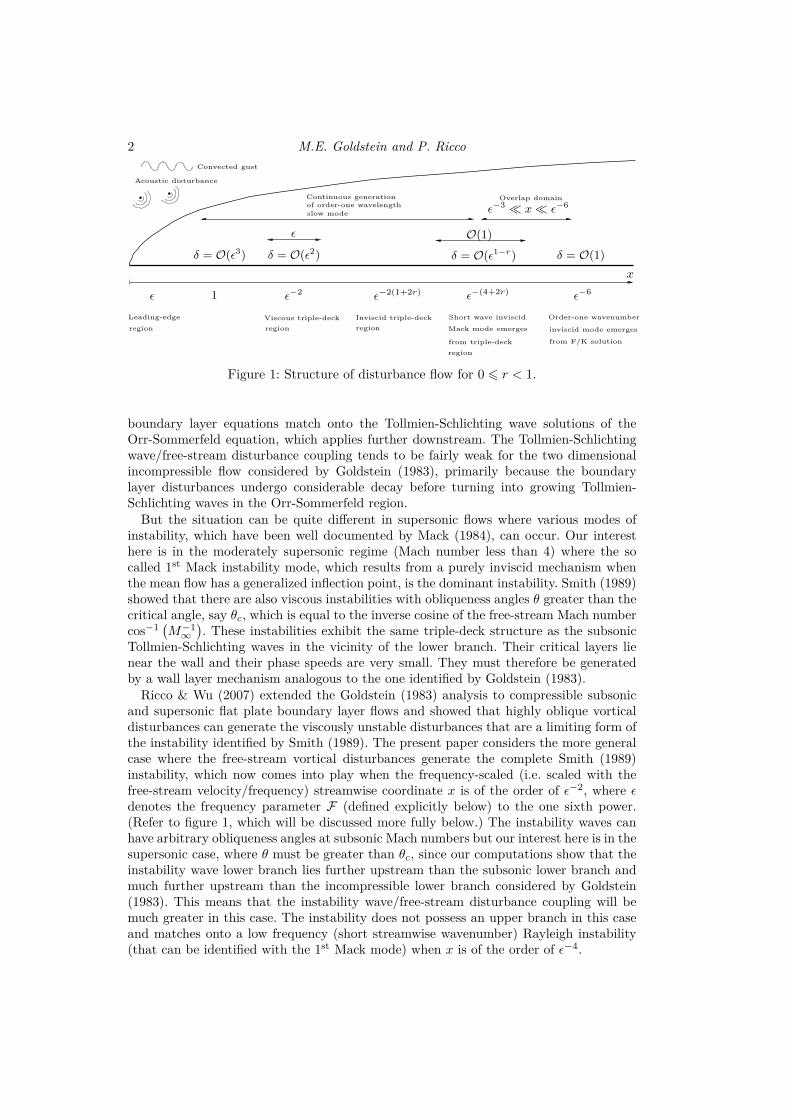
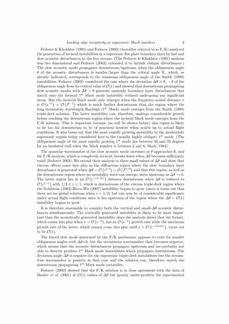
Figure 1: Structure of disturbance flow for 0 6 r < 1.
boundary layer equations match onto the Tollmien-Schlichting wave solutions of theOrr-Sommerfeld equation, which applies further downstream. The Tollmien-Schlichtingwave/free-stream disturbance coupling tends to be fairly weak for the two dimensionalincompressible flow considered by Goldstein (1983), primarily because the boundarylayer disturbances undergo considerable decay before turning into growing Tollmien-Schlichting waves in the Orr-Sommerfeld region.
But the situation can be quite different in supersonic flows where various modes ofinstability, which have been well documented by Mack (1984), can occur. Our interesthere is in the moderately supersonic regime (Mach number less than 4) where the socalled 1st Mack instability mode, which results from a purely inviscid mechanism whenthe mean flow has a generalized inflection point, is the dominant instability. Smith (1989)showed that there are also viscous instabilities with obliqueness angles θ greater than thecritical angle, say θc, which is equal to the inverse cosine of the free-stream Mach numbercos−1
(M−1
∞
). These instabilities exhibit the same triple-deck structure as the subsonic
Tollmien-Schlichting waves in the vicinity of the lower branch. Their critical layers lienear the wall and their phase speeds are very small. They must therefore be generatedby a wall layer mechanism analogous to the one identified by Goldstein (1983).
Ricco & Wu (2007) extended the Goldstein (1983) analysis to compressible subsonicand supersonic flat plate boundary layer flows and showed that highly oblique vorticaldisturbances can generate the viscously unstable disturbances that are a limiting form ofthe instability identified by Smith (1989). The present paper considers the more generalcase where the free-stream vortical disturbances generate the complete Smith (1989)instability, which now comes into play when the frequency-scaled (i.e. scaled with thefree-stream velocity/frequency) streamwise coordinate x is of the order of ǫ−2, where ǫdenotes the frequency parameter F (defined explicitly below) to the one sixth power.(Refer to figure 1, which will be discussed more fully below.) The instability waves canhave arbitrary obliqueness angles at subsonic Mach numbers but our interest here is in thesupersonic case, where θ must be greater than θc, since our computations show that theinstability wave lower branch lies further upstream than the subsonic lower branch andmuch further upstream than the incompressible lower branch considered by Goldstein(1983). This means that the instability wave/free-stream disturbance coupling will bemuch greater in this case. The instability does not possess an upper branch in this caseand matches onto a low frequency (short streamwise wavenumber) Rayleigh instability(that can be identified with the 1st Mack mode) when x is of the order of ǫ−4.
Leading edge receptivity at supersonic Mach numbers 3
Fedorov & Khokhlov (1991) and Fedorov (2003) (hereafter referred to as F/K) analyzedthe generation of inviscid instabilities in a supersonic flat plate boundary layer by fast andslow acoustic disturbances in the free stream. (The Fedorov & Khokhlov (1991) analysiswas two dimensional and Fedorov (2003) extended it to include oblique disturbances.)The slow acoustic mode propagates downstream/upstream when the obliqueness angleθ of the acoustic disturbances is smaller/larger than the critical angle θc, which, asalready indicated, corresponds to the minimum obliqueness angle of the Smith (1989)instabilities. Fedorov (2003) considered the case where the deviation ∆θ ≡ θc − θ of theobliqueness angle from its critical value is O(1) and showed that downstream propagatingslow acoustic modes with ∆θ > 0 generate unsteady boundary layer disturbances thatmatch onto the inviscid 1st Mack mode instability without undergoing any significantdecay. But the inviscid Mack mode only emerges when the frequency-scaled distance xis O
(ǫ−6)
= O(F−1
)which is much further downstream than the region where the
long streamwise wavelength Rayleigh (1st Mack) mode emerges from the Smith (1989)triple-deck solution. The latter instability can, therefore, undergo considerable growthbefore reaching the downstream region where the inviscid Mack mode emerges from theF/K solution. This is important because (as will be shown below) this region is likelyto lie too far downstream to be of practical interest when scaled up to actual flightconditions. It also turns out that the most rapidly growing instability in the moderatelysupersonic regime being considered here is the (usually highly oblique) 1st mode. (Theobliqueness angle of the most rapidly growing 1st mode lies between 50 and 70 degreesfor an insulated wall when the Mach number is between 2 and 6, Mack, 1984).
The spanwise wavenumber of the slow acoustic mode increases as θ approaches θc andthe F/K analysis, which is completely inviscid, breaks down when ∆θ becomes sufficientlysmall (Fedorov 2003). We extend their analysis to these small values of ∆θ and show thatviscous effects come into play in the diffraction region where the slow boundary layerdisturbance is generated when ∆θ = O
(ǫ2/3
)= O
(F1/9
)and that this region, as well as
the downstream region where an instability wave can emerge, move upstream as ∆θ → 0.The latter region lies at an O
(ǫ−(4+2r)
)distance downstream when ∆θ is reduced to
O(ǫ1−r
)with 1/3 6 r < 1, which is downstream of the viscous triple-deck region where
the Goldstein (1983)-Ricco-Wu (2007) instability begins to grow (since it turns out thatthere are no global solutions when r < 1/3) but can now be of considerable significanceunder actual flight conditions since it lies upstream of the region where the ∆θ = O(1)instability begins to grow.
It is therefore reasonable to consider both the vortical and small-∆θ acoustic distur-bances simultaneously. The vortically generated instability is likely to be more impor-tant than the acoustically generated instability since the analysis shows that the former,which comes into play when x = O
(ǫ−2), has an O
(ǫ−1)
growth rate while the maximum
growth rate of the latter, which cannot come into play until x = O(ǫ−(4+2r)
), turns out
to be O(1).
The forced slow mode generated by the F/K mechanism appears to exist for smallerobliqueness angles with ∆θ<0, but the streamwise wavenumber then becomes negative,which means that the acoustic disturbances propagate upstream and are probably notable to directly produce 1st Mack mode instabilities which propagate downstream. Thedeviation angle ∆θ is negative for the supersonic triple-deck instabilities but the stream-wise wavenumber is positive in that case and the solution can, therefore, match thedownstream propagating 1st Mack mode instability.
Fedorov (2003) showed that the F/K solution is in close agreement with the data ofMaslov et al. (2001) at O(1) values of ∆θ but greatly under-predicts the experimental
4 M.E. Goldstein and P. Ricco
receptivity coefficient when ∆θ is close to zero, which could be due the additional inviscidinstability that evolves from the viscous triple-deck solution.
As noted above, the present paper is concerned with the unsteady flow in a flat plateboundary layer generated by mildly oblique vortical disturbance and small-∆θ acousticdisturbances in a moderate supersonic Mach number free stream. It shows, among otherthings, that the vortical disturbances generate a viscous instability that can exhibit muchless decay upstream of its lower branch than the corresponding two dimensional subsonicmodes considered by Goldstein (1983) even when the frequency parameter is small andthat the resulting instabilities could, therefore, dominate over those generated by theacoustic disturbances. The relevant experiments are usually conducted with a trailingedge flap that tends to move the leading edge stagnation point to the lower surface of theplate, which could certainly cause the leading edge boundary layer to be slightly differentfrom the Blasius boundary layer considered in the paper and thereby slightly modify theleading edge receptivity. But the present paper is meant to explain the relevant physicsand we believe that this is best done by analyzing the ideal situation that the experimentsare meant to simulate.
The outline of the paper is as follows. The imposed upstream disturbance environ-ment is discussed in §2 and the upstream boundary layer flow generated by the imposedvortical disturbances is analyzed in §3.1. Section 3.2 describes the resulting asymptoticeigensolutions produced by this flow. The slow boundary layer disturbances generated byacoustic disturbances with obliqueness angles close to the critical angle are analyzed in§4. Section 5 shows that the vortically-generated asymptotic eigensolutions evolve intooblique instability waves with viscous triple-deck structure when, as noted above, thescaled streamwise coordinate is O(ǫ−2) while the acoustically-generated slow boundarydisturbances do not evolve into oblique instability waves in this region and eventually de-velop into oblique stable disturbances with inviscid triple-deck structure when the scaledstreamwise coordinate becomes O
(ǫ−(2+4r)
), 1/3 6 r < 1. Section 6 shows that both the
vortically-generated instability and the acoustically generated oblique disturbance even-tually evolve into modified Rayleigh-type instabilities at larger downstream distances.The numerical procedures are described in §7. The numerical results are presented in §8and their physical implications are discussed. Some final conclusions are given in §9.
2. Formulation
We consider a supersonic flow of an ideal gas with uniform free-stream velocity U∗∞,
temperature T ∗∞, dynamic viscosity µ∗
∞, and density ρ∗∞ past an infinitely thin flat plate
and suppose that a small amplitude harmonic distortion with angular frequency ω∗ issuperimposed on the flow. We also suppose that the time t is normalized by ω∗, thevelocities by U∗
∞, the pressure fluctuation by ρ∗∞ (U∗
∞)2, the temperature by T ∗
∞, and thedynamic viscosity by µ∗
∞. We let {x, y, z} denote Cartesian coordinates normalized byL∗ ≡ U∗
∞/ω∗ with the coordinate y being perpendicular to the surface of the plate.
As indicated in the introduction the present paper assumes the Reynolds numberρ∗U∗
∞L∗/µ∗∞ to be large and uses asymptotic theory to explain how the imposed har-
monic distortion generates oblique instabilities at large downstream distances in theviscous boundary layer that forms on the surface of the plate. The distortion will there-fore be inviscid at lowest approximation and, as is well known (Kovasznay 1953), canbe decomposed into an acoustic component that carries no vorticity, and vortical andentropic components that produce no pressure fluctuations.
Leading edge receptivity at supersonic Mach numbers 5
We only consider the first two for simplicity. The vortical velocity uv is given by
uv = {uv, vv, wv} = δ{u∞, v∞, w∞} exp [i(x − t + γy + βz)] , (2.1)
where δ ≪ 1 and u∞, v∞, w∞ satisfy the continuity condition
u∞ + γv∞ + βw∞ = 0 (2.2)
but are otherwise arbitrary constants while the acoustic component is governed by thelinear wave equation which has a fundamental plane wave solution
{ua, pa} = {ua, va, wa, pa} =δp∞
1 − α{α, γ, β, 1 − α} exp [i(αx + γy + βz − t)] , (2.3)
for the velocity and pressure perturbation where
γ =√
(M2∞ − 1) (α − α1)(α − α2), α1,2 =
M2∞ ±
√M2
∞ + β2 (M2∞ − 1)
M2∞ − 1
, (2.4)
where, as noted in the introduction, M∞ denotes the free-stream Mach number.The leading edge interaction will produce large scattered fields when the incidence
angle tan−1(va/ua) = tan−1(γ/α) of the acoustic wave and tan−1(vv/uv) of the vorticaldisturbance are O(1). And, in order to avoid this complication, we only consider the casewhere the incidence angle of the vortical disturbance is small, which requires that
v∞
u∞
≪ 1 (2.5)
and the case where the incidence angle of the acoustic disturbance is zero, which requiresthat
α = α∓ =M∞ cos θ
M∞ cos θ ∓ 1, θ ≡ tan−1
(β
α
), (2.6)
where the subscripts −/+ refer to the slow/fast acoustic modes. Equation (2.6) showsthat the slow mode wavenumber becomes infinite when the obliqueness angle is equal tothe critical angle referred to in the introduction.
As indicated above our interest here is in explaining how the incident harmonic distor-tions generate oblique instabilities at large downstream distances in the viscous boundarylayer where the mean temperature, density, and streamwise velocity, say T , ρ, U , respec-tively, can be expressed as functions of the Dorodnitsyn-Howarth variable
η ≡ 1
ǫ3√
2x
∫ y
0
ρ (x, y) dy (2.7)
and determined from the similarity equations (Stewartson 1964)
U = F ′(η), (2.8)
(µF ′′
T
)′
+ FF ′′ = 0, (2.9)
Pr−1
(µT ′
T
)′
+ FT ′ + (γr − 1) M2∞(F ′′)2 = 0, (2.10)
ρT = 1, (2.11)
F (0) = F ′(0) = 0, T ′(0) = 0; F ′ → 1, T → 1 as η → ∞, (2.12)
where γr is the specific heat ratio and the mean viscosity µ is assumed to depend on the

6 M.E. Goldstein and P. Ricco
temperature. The prime is used to denote differentiation with respect to η and Pr is usedto denote the Prandtl number.
The natural small parameter for the asymptotic expansion turns out to be
ǫ ≡ F1/6, (2.13)
where, as indicated in the introduction,
F ≡ ω∗µ∗∞
ρ∗∞ (U∗
∞)2 (2.14)
denotes the frequency parameter. We begin by considering the unsteady flow generatedby the upstream vorticity.
3. Boundary layer disturbances generated by free-stream vorticity
3.1. Leading edge region
Our interest here is in boundary layer disturbances that generate oblique viscous insta-bilities in a triple-deck region that lies at an O
(ǫ−2)
distance downstream, which, as will
be shown below, will have O(ǫ−1)
spanwise wavenumbers. And we therefore require that
β ≡ ǫβ = O(1) (3.1)
since the spanwise wavenumber must remain constant as the disturbances propagatedownstream. The continuity condition (2.2) will then require that
w∞ ≡ w∞
ǫ= O(1) (3.2)
and the obliqueness requirement (2.5) can be satisfied if we require that
v∞ ≡ v∞
ǫ= O(1). (3.3)
Equation (2.2) then becomes
u∞ + γ v∞ + βw∞ = 0, (3.4)
where
γ ≡ ǫγ = O(1). (3.5)
The vortical velocity (2.1) will then interact with the plate to produce the followinginviscid velocity field (Ricco & Wu 2007)
uv(x, y, z) =δ
{u∞eiγy/ǫ + iǫ2 v∞
ge−gy/ǫ, ǫv∞
(eiγy/ǫ − e−gy/ǫ
),
ǫ
(w∞eiγy/ǫ + iv∞
β
ge−gy/ǫ
)}ei(x−t+βz/ǫ),
(3.6)
g ≡ ǫ
√
1 +
(β
ǫ
)2
= β +ǫ2
2β+ ... (3.7)
when the streamwise coordinate x is assumed to be large enough so that the leading edgerefraction effects have decayed.
As noted above the free-stream disturbance (2.1) generates a slip velocity at the surfaceof the plate that must be brought to zero in a thin viscous boundary layer whose meanvelocity and temperature are given by (2.7)-(2.12). We begin by considering the flow in

Leading edge receptivity at supersonic Mach numbers 7
the vicinity of the leading edge where the streamwise length scale is x = O(1). Since(3.6) depends on the streamwise coordinate only through this relatively long streamwiselength scale, the solution {u, v, w, ϑ} for the velocity and temperature in this region isgiven by (Ricco & Wu 2007)
{u, v, w, ϑ} =
{F ′(η),
ǫ3T√2x
(ηcF ′ − F ) , 0, T
}+
δ{
u0(x, η), ǫ3√
2xv0(x, η), ǫw0(x, η), ϑ0(x, η)}
ei(βz/ǫ−t),
(3.8)
where
ηc ≡ 1
T (η)
∫ η
0
T (η)dη (3.9)
and{
u0(x, η), ǫ3√
2xv0(x, η), ǫw0(x, η), ϑ0(x, η)}
is determined by the linearized bound-
ary layer equations. The solution{
u0, v0, w0, ϑ0
}to these equations can be divided into
the following two components (Gulyaev et al. 1989)
{u0, v0, w0, ϑ0
}=
(u∞eiγy/ǫ + iǫ2 v∞
ge−gy/ǫ
){u, v, 0, ϑ
}+
iβ
(w∞eiγy/ǫ + iv∞
β
ge−gy/ǫ
){u(0), v(0), w(0), ϑ
(0)}
,
(3.10)
where{
u(0), v(0), w(0), ϑ(0)}
satisfy the three-dimensional compressible linearized bound-
ary layer equations subject to the boundary conditions (Ricco & Wu 2007)
u(0) → 0, w(0) → eix, ϑ(0) → 0 as η → ∞, (3.11)
while the two-dimensional solution {u, v, 0, ϑ} satisfies the two-dimensional linearizedboundary layer equations
−iu+F ′ ∂u
∂x− F
2x
∂u
∂η−ηcF ′′
2xu+
F ′′
Tv+
1
2x
(F − ∂µ′
∂η
)(F ′′
Tϑ
)=
1
2x
∂
∂η
(µ
T
∂u
∂η
), (3.12)
∂u
∂x− ηcT
2x
∂
∂η
(u
T
)+
∂
∂η
(v
T
)+
(i − F ′ ∂
∂x+
F
2x
∂
∂η
)(ϑ
T
)= 0, (3.13)
− ηcT ′
2xu − 2M2
∞(γr − 1)F ′′
2x
∂u
∂η+
T ′v
T−[
i − T ′F
2xT+
1
2xPr
(µ′T ′
T
)′
+M2
∞(γr − 1)(F ′′)2
2xT
]ϑ +
[F ′ ∂
∂x− 1
2x
(F +
µ′T ′
PrT
)∂
∂η
]ϑ − 1
2xPr
∂
∂η
(µ
T
∂ϑ
∂η
)= 0
(3.14)
(where µ′ denotes dµ/dT ) subject to the boundary conditions
u → eix, w, ϑ → 0 as η → ∞. (3.15)
The estimate (5.18) below suggests that the lowest order triple-deck solution consideredin §5 will match onto the viscous quasi-two dimensional solution {u, v, 0, ϑ}, where thespanwise dependence only enters parametrically through the exponential factor in (3.8).
8 M.E. Goldstein and P. Ricco
3.2. Asymptotic eigensolutions
Prandtl (1938), Glauert (1956), and Lam & Rott (1960) showed that
u(x, η) = −B(x)F ′′(η)√2xT
, v(x, η) = iB(x) +dB
dxF ′(η) − B(x)ηcF ′′(η)
2x, (3.16)
ϑ(x, η) = −B(x)T ′(η)√2xT
(3.17)
is an exact eigensolution of the two-dimensional linearized unsteady boundary layer equa-tions (3.12)-(3.14) that satisfies the homogeneous boundary conditions u, w, ϑ → 0 asη → ∞ for all B(x), but does not necessarily satisfy the no-slip condition at the wall.Lam & Rott (1960) showed that (3.12)-(3.14) also possess asymptotic eigensolutions thatemerge at large values of x and satisfy a no-slip condition at the wall but only consideredthe incompressible limit. These solutions have a double layer structure which consists ofan outer region that encompasses the main part of the boundary layer and a thin viscouswall layer. They showed that the solution in the outer region is still given by (3.16) and(3.17) but with the arbitrary function B(x) determined by matching with the flow in theviscous wall layer. Ricco & Wu (2007) pointed out that their analysis will also apply tothe compressible case provided the full compressible solution (3.16) and (3.17) is used inthe outer region and the solution in the viscous wall layer is slightly modified to accountfor the temperature and viscosity variations. The end result is that the function B(x)will now be given by
B(x) = x3/2Bn exp
[−23/2eiπ/4
3λζ3/2n
(Tw
µw
)1/2
x3/2
]+ ... (3.18)
where ζn is a root of
Ai′ (ζn) = 0, for n = 0, 1, 2, 3... (3.19)
and
λ ≡ F ′′(0). (3.20)
The only difference from the Lam-Rott result is the (Tw/µw)1/2
factor in the exponent.The asymptotic solution to the full inhomogeneous boundary value problem (3.12)-(3.15)can now be expressed as the sum of a Stokes layer solution plus a number of theseasymptotic eigensolutions. Goldstein (1983) and Goldstein et al. (1983) showed how themultiplicative constants Bn can be determined from the full numerical solution to theboundary layer problem. But our primary interest here is in the lowest order n = 0solution because, as will be shown below, this is the one that will match onto a spa-tially growing oblique instability wave further downstream. The final result can then beused to relate the instability wave amplitude to the initial amplitude of the free-streamdisturbance, i.e. to solve the receptivity problem.
The three-dimensional linearized boundary layer equations could also have quasi-two dimensional asymptotic eigensolutions which satisfy equations (3.12)-(3.14) and thepresent result will apply to those solutions as well. Both sets of eigensolutions will haveto be considered when the full receptivity problem is solved. These boundary layer dis-turbances will, as already noted, eventually evolve into a spatially growing instability ina region that lies further downstream. But we first consider the boundary layer distur-bances generated by the free-stream acoustic waves.
Leading edge receptivity at supersonic Mach numbers 9
4. Boundary layer disturbances generated by the Fedorov/Khokhlovmechanism for obliqueness angles close to critical angle
F/K analyzed the generation of Mack mode instabilities in flat plate boundary layersby oblique acoustic waves of the form (2.3) where the wavenumbers α and β satisfythe dispersion relation (2.6) when the incidence angle γ is equal to zero, which, forreasons given in §2, is the case of interest here. The focus of the present paper is onthe moderate supersonic regime (the Mach number is less than about 4) where the mostrapidly growing disturbances are usually highly oblique 1st Mack modes. (As indicatedabove, the obliqueness angle of the most rapidly growing 1st mode lies between 50 and70 degrees for an insulated wall when the Mach number is between 2 and 6, Mack1984). F/K showed that diffraction of the slow acoustic wave by the nonparallel meanboundary layer flow can produce a 1st Mack mode instability in the downstream regionwhere x = O
(ǫ−6)
when its obliqueness angle theta is less than the critical angle
cos θc ≡ 1
M∞
(4.1)
and the deviation
∆θ ≡ θc − θ (4.2)
is O(1). Their analysis shows that the diffraction occurs in the downstream region wherex = O
(ǫ−3)
and the unsteady flow has a three layer structure: a passive Stokes layer nearthe wall, a main boundary layer region that fills the mean boundary layer and an outerdiffraction region of thickness O
(ǫ−3/2
). The instability emerges from the downstream
limit of the solution in this region.As noted above our interest here is in comparing the unstable flow produced by this
mechanism with that produced by the vortical disturbances. It is natural to do thiscomparison at the same scaled spanwise wavenumber and scaled time (and, therefore,the same period for the periodic motion being considered here). But, as noted above, thevortical disturbances must have large spanwise wavenumber β in order to produce obliqueinstability waves in the downstream region. The corresponding acoustic disturbances willonly have large spanwise wavenumbers when their obliqueness angles θ are close to thecritical angle θc, i.e. when ∆θ ≪ 1. And since
cos (θc − ∆θ) = cos θc + ∆θ sin θc + O(
(∆θ)2)
, (4.3)
tan (θc − ∆θ) = tan θc − ∆θ
cos θc+ O
((∆θ)
2)
, (4.4)
when ∆θ ≪ 1, it follows from (2.6) that
β = β1 =β
∆θ(4.5)
and
α =α
∆θ+ α1 + ..., (4.6)
where
α =1
tan θc, β = 1, α1 =
1
sin2θc(4.7)
are O(1) constants when this occurs. This shows that α also becomes large when ∆θ ≪ 1and that α will expand in powers of ∆θ as indicated in (4.6), if β is fixed at (4.5) toall orders in ∆θ (which we now assume to be the case). But the F/K diffraction region
10 M.E. Goldstein and P. Ricco
equations do not provide an appropriate asymptotic balance when ∆θ ≪ 1 and newequations have to be derived before that analysis can be extended into the small-∆θregime. The relevant equations are derived in this section.
We begin by rescaling the F/K diffraction region equations. F/K showed that the∆θ = O(1) solution, say {u, v, w, ϑ, p}, for the velocity, temperature and pressure in theouter diffraction region (region 2 in their notation) is of the form
{u, v, w, ϑ, p} ={1, 0, 0, 1, 1} + δ{
u2(x2, y2), ǫ3/2v2(x2, y2), w2(x2, y2), ϑ2(x2, y2),
p2(x2, y2)} exp
{i
[(α
∆θ+ α1
)x +
βz
∆θ− t
]},
(4.8)
where
x2 ≡ xǫ3 = O(1), y2 ≡ yǫ3/2 = O(1) (4.9)
and the pressure is determined by
∂2p2
∂y22
= 2i[M2
∞(α − 1) − α] ∂p2
∂x2, (4.10)
subject to the boundary conditions
p2(x2, ∞) = p2(0, y2) = 1, (4.11)
∂p2
∂y2= −i(α − 1)v1(x2, ∞), p2 = p1(x2) at y2 = 0, (4.12)
where the wall normal velocity v1(x2, ∞)=limη→∞ v1(x2, η) is determined by the solutionin the boundary layer where η = O(1). This solution shows that v1(x2, ∞) is related tothe boundary layer pressure p1 by
v1(x2, ∞) =iαk
cos2 θ
√x2p1, (4.13)
where k is a constant.Equations (4.10) and (4.12) become
∂2p2
∂y22
= 2iα(M2
∞ − 1) ∂p2
∂x2, (4.14)
∂p2
∂y2= −iαv1(x2, ∞), p2 = p1(x2) at y2 = 0 (4.15)
when the obliqueness angle is close to the critical angle. But, as noted above, theseequations have to be rescaled in order to obtain an asymptotically balanced result becausenow α ≫ 1. Appendix A shows that they will remain unchanged, i.e. they can be writtenas
∂2p2
∂ ˜y22
= 2iα(M2
∞ − 1) ∂p2
∂ ˜x2, (4.16)
∂p2
∂ ˜y2
= −iαv1
(˜x2, ∞
), p2 = p1
(˜x2
)at ˜y2 = 0, (4.17)
v1
(˜x2, ∞
)=
iαk(˜x2
)
cos2 θ
√˜x2p2, (4.18)
Leading edge receptivity at supersonic Mach numbers 11
if we put
˜x2 ≡ x2
(∆θ)3/2
∆ϕ=
xǫ3
(∆θ)3/2
∆ϕ,
˜y2 ≡ y2
(∆ϕ)5/4
(∆θ)1/2
= O(1), k(˜x2
)≡ k∆ϕ,
(4.19)
where we now allow the rescaled proportionality constant k(˜x2
)to depend on ˜x2 in
order to accommodate the altered boundary layer flow which determines (4.18). Thescale factor ∆ϕ ≪ 1 is introduced to account for the fact this flow now develops a doublelayer structure below the outer diffraction region when ∆θ → 0: a main boundary layerwhere η = O(1) and a wall layer where
η ≡ η
∆ϕ= O(1). (4.20)
The solution to (4.16), which is essentially the same as that in F/K, implies that the wallboundary condition (4.17) can be written as
p2
(˜x2, 0
)= 1 −
˜x2√2πiα (M2
∞ − 1)
∫ 1
0
i√
σ√σ − 1
α
[v1
(˜x2σ, ∞
)√
˜x2σ
]dσ. (4.21)
It turns out that the wall layer flow can be balanced if the lowest order solution {u, v, w, p}in the main boundary layer behaves like
{u, v, w, p} ={U(η), 0, 0, 1} + δ
u1
(˜x2, η
)
∆ϕ,
[ǫ3
(∆θ)1/2
∆ϕ
]1/2
v1
(˜x2, η
), w1
(˜x2, η
),
p1
(˜x2
)}exp
{i
[(α
∆θ+ α1
)x + βz − t
]},
(4.22)
with
v1 = iαU(η)A(˜x2
)√2˜x2 and u1 = −U ′(η)A
(˜x2
)
T (η). (4.23)
The wall layer flow will be completely viscous when the convective and viscous terms inthe wall layer equations, which are proportional to αη and (2x)−1∂2/∂η2 respectively,are of the same order. This occurs when
α
(∆ϕ
∆θ
)= O
(1
2x (∆ϕ)2
)(4.24)
or
x = O(
∆θ
(∆ϕ)3
)(4.25)
and, since ˜x2 = O(1), it follows from (4.19) that this occurs when
∆ϕ =
[ǫ3
(∆θ)1/2
]1/4
(4.26)
12 M.E. Goldstein and P. Ricco
or equivalently when
∆ϕ
∆θ=
(ǫ2/3
∆θ
)9/8
. (4.27)
Inserting (4.26) into (4.19) shows that
˜x2 ≡ x2
ǫ3/4 (∆θ)11/8
=xǫ9/4
(∆θ)11/8
= xǫ4/3
(ǫ2/3
∆θ
)11/8
= x
[ǫ6
(∆θ)11/3
]3/8
,
˜y2 ≡ y2
(∆θ)31/64
ǫ15/16.
(4.28)
The distinguished limit corresponds to the case where the wall layer flow is also timedependent. This occurs when ∆ϕ = ∆θ or, in view of equation (4.27), when ∆θ =O(ǫ2/3
). The corresponding wall layer solution, which is given in Appendix B, shows that
the wall normal velocity v1
(˜x2, ∞
)=limη→∞ v1(˜x2, η) is given in terms of the integral∫∞
ξ0Ai(ξ)dξ and the derivative Ai′(ξ0) of the Airy function Ai(ξ0) by
v1
(˜x2, ∞
)√
2˜x2
= ip1
(˜x2
) (α2 + β2)
T 2wξ0
λAi′ (ξ0)
∫ ∞
ξ0
Ai (ξ) dξ, (4.29)
which behaves like
v1
(˜x2, ∞
)√
2˜x2
∼ − ip1
(˜x2
) (α2 + β2
)T 2
w
λ(4.30)
as ˜x2 → ∞ since (Abramowitz & Stegun 1964, pp. 446-447)
Ai′(ξ0)∫∞
ξ0Ai(q)dq
→ −ξ0 as ξ0 → ∞. (4.31)
Inserting (4.17) and (4.30) into (4.21) shows that
p1
(˜x2
)= 1 − γ0
∫ 1
0
√σ√
1 − σp(σ ˜x2
)dσ, (4.32)
where
γ0 ≡˜x2
(α2 + β2
)α1/2T 2
w
λ√
2πi (M2∞ − 1)
, (4.33)
which is formally the same as the equation considered by F/K who showed that thesolution is given by
p1
(˜x2
)∼ exp
[γ2
0π(˜x2
)2]
as ˜x2 → ∞. (4.34)
This result also applies when
ǫ2/3
∆θ= ǫr, 0 < r < 2/3. (4.35)
But the wall layer flow will be inviscid when ∆θ > ǫ2/3 and the time dependent termmust again balance the convective term in the wall layer equations, which means thatthe wall layer scale factor ∆ϕ must also be set equal to ∆θ in this case. Equation (4.19)then becomes
˜x2 ≡ x2
(∆θ)5/2
=xǫ3
(∆θ)5/2
= O(1), ˜y2 ≡ y2
(∆θ)7/4
= O(1), k ≡ k∆θ, (4.36)
Leading edge receptivity at supersonic Mach numbers 13
which is consistent with equation (4.28) when ∆θ = ǫ2/3 and shows that the diffractionregion moves upstream when ∆θ → 0. The expansion breaks down when the length of the
diffraction region x = (∆θ)5/2 ˜x2ǫ−3 is equal to the wavelength ∆θ when ∆θǫ−2 = O(1).
Equation (4.27) shows that ∆ϕ (∆θ)−1 ≫ 1 when ǫ2/3 (∆θ)
−1 ≫ 1. This implies that
the time dependent terms will drop out of the wall layer equations when ǫ2/3 (∆θ)−1 ≫ 1,
which occurs when ξ is replaced by ξ in the analysis of Appendix B. The relevant solutionfor the wall normal velocity v1 can therefore be obtained from equation (4.29) by takingthe limit ξ0 → 0, with p1, ξ0 held fixed. And, since (Abramowitz & Stegun 1964, pp.448-449)
∫∞
ξ0Ai (ξ) dξ
Ai′ (ξ0)→ −Γ(1/3)
32/3as ξ0 → 0, (4.37)
where Γ(x) denotes the Gamma function, it follows that
v1
(˜x2, ∞
)√
2˜x2
= − ip1
(˜x2
) (α2 + β2)
T 2wξ0Γ(1/3)
32/3λ= ip1
(˜x2
) (α2 + β2
)
× T 2wi1/3
[Γ(1/3)
32/3λ
](√2˜x2
αλ
)2/3(Tw
µw
)1/3
.
(4.38)
And inserting (4.17) and (4.38) into (4.21) shows that
p2 = 1 −(˜x2
)4/3γ1
∫ 1
0
√σ
1 − σσ1/3p2
(˜x2σ)
dσ, (4.39)
where
γ1 ≡(α2 + β2
)T 2
w
21/3Γ(1/3)
λ5/332/3√
iπα (M2∞ − 1)
(iTwα
µw
)1/3
(4.40)
is a constant.Equation (4.39) possesses a power series solution of the form
p2 =∞∑
n=0
anZn, (4.41)
where
Z ≡ γ1
(˜x2
)4/3 √π, (4.42)
which is somewhat different from the corresponding solution obtained by F/K. Inserting(4.42) into (4.39), equating coefficients of like powers of Z, summing the resulting recur-rence relation and using equation 6.1.8, 6.2.1 and 6.2.2 of Abramowitz & Stegun (1964)shows that
an =
n∏
j=1
Γ(4j/3 + 1/2)
Γ(4j/3 + 1). (4.43)
It therefore follows from equations (4.42) and (C.5) that
p1 ∼ 3
4A(8π)1/4
√πγ1
(˜x2
)4/3exp
[3γ2
1π(˜x2
)8/3
8
]as ˜x2 → ∞, (4.44)
where γ1 is given by (4.40). Equations (4.17) and (4.22) show that the pressure p(˜x2
)in

14 M.E. Goldstein and P. Ricco
the main boundary layer is given by
p(˜x2
)− 1 = δp1
(˜x2
)exp
{i
[(α
∆θ+ α1
)x +
βz
∆θ− t
]}. (4.45)
The acoustically generated boundary layer disturbance considered in this section aswell as the vortically generated disturbance considered in §3 will eventually evolve intopropagating eigensolutions in regions that lie further downstream. The resulting flowwill have a triple-deck structure of the type considered by Smith (1989), Wu (1999),and Ricco & Wu (2007) in the latter (i.e. vortically generated) case. But the acousticallygenerated disturbance considered in the present section can also potentially have a triple-deck structure when ∆θ = O(ǫ). We therefore begin by considering the flow in this regionand show that the resulting triple-deck solution will match onto the compressible Lam-Rott eigensolutions (3.16) and (3.17). We then further investigate whether an analogousmatching occurs for the acoustically generated small-∆θ F/K solution.
5. The triple-deck region
As shown by Smith (1989), Wu (1999), and Ricco & Wu (2007) the linearized Navier-Stokes equations possess an eigensolution of the form
{u, v, w, p} = δΦ(y, ǫ) exp
{i
[1
ǫ3
∫ x1
0
κ (x1, ǫ) dx1 + βz − t
]}(5.1)
in the triple-deck region where
x1 ≡ ǫ2x = O(1) (5.2)
and
z ≡ z
ǫ=
z∗ω∗
ǫU∗∞
(5.3)
is a scaled transverse coordinate and, as noted in Goldstein (1983), κ has the expansion
κ (x1, ǫ) = κ0 (x1) + ǫκ1 (x1) + ǫ2κ2 (x1) + ..., (5.4)
where the lowest order term in this expansion satisfies the following dispersion relation
κ20 + β
2=
1
(iκ0)1/3
(λ√2x1
)5/3(µw
T 7w
)1/3
[β
2 −(M2
∞ − 1)
κ20
]1/2
Ai′ (ξ0)∫∞
ξ0Ai (q) dq
(5.5)
and
ξ0 = −i1/3
(√2x1
κ0λ
)2/3(Tw
µw
)1/3
, (5.6)
which is easily obtained by rewriting equation (5.2) of Ricco & Wu (2007) or equation(3.17) of Wu (1999) in the present notation.
The solution in the main boundary layer where η = O(1) is given by
{u, v, w, p} =δ
{A (x1) U ′(η)
T (η), −iκ0A (x1) U (η)
√2x1, −ǫ2β PT (η)
κ0U(η), ǫ2P
}
× exp
{i
[1
ǫ
∫ x
0
κ (x1, ǫ) dx + βz − t
]},
(5.7)
where δ ≪ 1 is the common scale factor used in (3.6).

Leading edge receptivity at supersonic Mach numbers 15
The solution in the upper deck where
y ≡ y
ǫ=
y∗ω∗
ǫU∗∞
= O(1) (5.8)
is given by
p = δp(2) exp
{−[β
2 −(M2
∞ − 1)
κ20
]1/2
y
}exp
{i
[1
ǫ
∫ x
0
κ (x1, ǫ) dx + βz − t
]},
(5.9)when the branch of the square root is chosen so that
ℜ{[
β2 −
(M2
∞ − 1)
κ20
]1/2}
> 0 (5.10)
in order to exclude solutions exhibiting unphysical wall normal exponential growth.Continuity of pressure and wall normal velocity requires that
p(2) = P ,∂p(2)
∂y= −
√2x1κ2
0A for y = 0 (5.11)
which implies that P and A are related by
[β
2 −(M2
∞ − 1)
κ20
]1/2
P = κ20
√2x1 A. (5.12)
The equation for w can be written as
w = δǫ2 κ0β√
2x1 AT (η)[β
2 − (M2∞ − 1) κ2
0
]1/2
U(η)
exp
{i
[1
ǫ
∫ x
0
κ (x1, ǫ) dx + βz − t
]}. (5.13)
As expected these equations reduce to equations (5.2) and (5.3) of Goldstein (1983) withH defined by the right hand side of (4.52) of that reference when β and M∞ are set tozero.
5.1. Matching with the Lam-Rott solution
Equations (5.5) and (5.6) can be satisfied at small values of x1 if κ0 ∼ √x1 and
ξ0 → ζn, for n = 0, 1, 2, ... as x1 → 0, (5.14)
where ζn is the nth root of (3.19). Inserting (5.14) into (5.5) shows that
κ0 → 1
λζ3/2n
(2Twx1
iµw
)1/2
as x1 → 0. (5.15)
Inserting (5.15) into (5.4) shows that (5.1) matches onto (3.16)-(3.19). Equation (5.13)then implies that
w ∼ δǫ2 2x1TA
Uas x1 → 0. (5.16)
It therefore follows from (5.7) that
w
u∼ ǫ2x1
λas x1 → 0 (5.17)
and, therefore, thatw
u= O
(ǫ4)
for x = O(1). (5.18)

16 M.E. Goldstein and P. Ricco
This shows that w drops out and the flow in the main deck becomes two dimensional asx1 → 0 and is therefore compatible with the quasi-two dimensional Lam-Rott solution(3.16)-(3.18).
5.2. Matching with the small-∆θ Fedorov/Khokhlov solution
As explained at the end of §4 it is necessary to investigate whether the acoustically-driven small-∆θ F/K solution matches onto the triple-deck instability downstream. Tothis end we note that the triple-deck dispersion relation (5.5)-(5.6) also has a solutionthat behaves like
κ0 → β
(M2∞ − 1)
1/2− β
11/3[α0(0)]
2x
5/31 + O
(x2
1
)as x1 → 0, (5.19)
where
α0(x) ≡ M2∞T 2
w(2i)1/3∫∞
xAi (q) dq
Ai′(x)λ5/3 (M2∞ − 1)
17/12(µw/Tw)
1/3=
(α2 + β2
)T 2
w(2iα)1/3∫∞
xAi (q) dq
Ai′(x)λ5/3 [α (M2∞ − 1)]
1/2(µw/Tw)
1/3
(5.20)and α is given by (4.6) and (4.7). It, therefore, follows that
1
ǫ3
∫ x1
0
[κ0 (x1) + ǫκ1 (x1)] dx1 → αx
∆θ− 3ǫ6 [α0(0)]
2x8/3
8 (∆θ)11/3
=
αx
∆θ− 3 [α0(0)]
2
8
x
[ǫ6
(∆θ)11/3
]3/8
8/3
=αx
∆θ− 3 [α0(0)]
2
8˜x
8/32
(5.21)
when β is set equal to ǫ/∆θ = O(1) and ˜x2 is given by (4.28), which shows that theF/K solution (4.44), (4.45) and (4.40) matches onto the pressure component of theouter triple-deck solution (5.7) when ∆θ = ǫ/β = O(ǫ) with the lowest order termin the expansion (5.4) determined by the Smith-Ricco-Wu dispersion relation (5.5),
which is only valid when[β
2 − (M2∞ − 1)κ2
0
]1/2
satisfies (5.10). But inserting (5.19)
into[β
2 − (M2∞ − 1)κ2
0
]1/2
shows that the real part of this quantity is less than zero,
which means that (5.10) is not satisfied and therefore that (5.5) is invalid. This showsthat there are no global solutions with obliqueness angles close to the critical angle thatextend (4.44) and (4.45) into the downstream region since these solutions would exhibitunphysical exponential growth in the wall normal direction.
It is therefore necessary to increase the magnitude of the critical angle deviation ∆θin the F/K solution (given in (4.22)) in order to construct a non-local solution that canbe extended downstream. This can be accomplished by putting ǫ/∆θ = O (ǫr) where ris required to lie in the range
0 < r < 1 (5.22)
since (as explained above) we want the deviation ∆θ of the obliqueness angle from thecritical angle to remain small in order to compare the result with the viscous triple-decksolution. Inserting the rescaled variables
β = β/ǫr, κ0 = κ0/ǫr, x1 = x1ǫ4r (5.23)
into (5.5), using (4.31) and taking the limit as ǫ → 0 with β, κ0 and x1 held fixed, shows

Leading edge receptivity at supersonic Mach numbers 17
that the rescaled wavenumber κ0 satisfies the inviscid dispersion relation
κ02 + β
2=
λ
[β
2−(M2
∞ − 1)
κ20
]1/2
κ0
√2x1T 2
w
(5.24)
when the square root
[β
2− (M2
∞ − 1)κ20
]1/2
is required to remain finite as ǫ → 0. It can
then be shown by direct substitution that the solution κ0 behaves like
κ0 → β
(M2∞ − 1)
1/2− β
5α2
0x1 as x1 → 0, (5.25)
where
α0 ≡ M2∞T 2
w
(M2∞ − 1)
7/4λ
. (5.26)
The square root
[β
2− (M2
∞ − 1)κ20
]1/2
now satisfies the inequality (5.10) when x1 → 0
and (5.24) therefore remains valid in this limit.The pressure component of the resulting solution (5.7) will then match onto the
downstream limit (4.33), (4.34) and (4.45) of the F/K diffraction region solution when
β = O(ǫ1−r/∆θ
)with 1/36r<1 and ˜x2 is given by (4.36) since it follows from (3.1),
(5.2), (5.23) that
1
ǫ3
∫ x1
0
κ0 (x1) dx1 =1
ǫ3(r+1)
∫ x1
0
κ0 (x1) dx1 →
αx
∆θ− ǫβ
5α2
0x2/2 =αx
∆θ− β
5α2
0
(ǫ3x)2
/2 =αx
∆θ− α2
0˜x
22/2.
(5.27)
We can investigate the remaining range ǫ < O (∆θ) < ǫ2/3 of ∆θ by noting that adifferent limiting form of equations (5.5) and (5.6) can be obtained when κ0 is allowed
to approach β/(M2
∞ − 1)1/2
as ǫ → 0. Inserting the first two of the rescaled variables(5.23) into these equations and putting
κ0 =β
(M2∞ − 1)1/2
− ǫ6r [a (x1)]2
(5.28)
where
x1 ≡ x1/ǫ2r (5.29)
shows that the resulting rescaled equations will be satisfied to lowest order in ǫ if we put
a (x1) ≡ M2∞β
11/6
(M2∞ − 1)
5/4
(√x1
λ
)5/3(iT 7
w
µw
)1/3∫∞
ξ0Ai (q) dq
Ai′ (ξ0)(5.30)
where
ξ0 = −i1/3
[√2 (M2
∞ − 1) x1
βλ
]2/3(Tw
µw
)1/3
. (5.31)
The asymptotic behavior of the upstream diffraction layer solution is given by (4.40),(4.44), and (4.45) when ∆θ < O
(ǫ2/3
). The resulting pressure component of the inviscid

18 M.E. Goldstein and P. Ricco
triple-deck solution (5.7) will match onto these equations when κ0 is given by (5.28)-(5.31) with β set equal to ǫ/∆θ since
a → M2∞β
11/6
(M2∞ − 1)
5/4
(√x1
λ
)5/3(iT 7
w
µw
)1/3 ∫∞
0Ai (q) dq
Ai′ (0)as x1 → 0 (5.32)
and it therefore follows that
1
ǫ3
∫ x1
0
κ0 (x1) dx1 =1
ǫ3+r
∫ x1
0
κ0 (x1) dx1 →
xα
∆θ− 3α2
0
8
{x[ǫ6/ (∆θ)
11/3]3/8
}8/3
=xα
∆θ− 3α2
0
8
(∆θ ˜x2
∆ϕ
)8/3
,
(5.33)
where α is given by (4.6) and (4.7) and α0 is an O(1) constant. But it follows from
(5.28) that the square root
[β
2−(M2
∞ − 1)
κ20
]1/2
does not satisfy (5.10) in this case,
which shows that a global solution does not exist when ∆θ = o(ǫ2/3
). The results of
this section therefore show that the small-∆θ F/K solution (4.45) only matches ontoa physically realizable inviscid triple solution when ǫ2/3 6 O (∆θ) < 1. This implies,among other things, that the former solution can only be continued downstream whenthe unsteady and convective terms both appear in the wall layer equations.
6. The next stage of evolution
It follows from (4.31), (5.5) and (5.6) that
β → 1
κ1/30 T 2
w
(λ√2x1
)5/3(√2x1
κ0λ
)2/3
=λ
κ0T 2w
√2x1
(6.1)
when x1 → ∞ and, therefore, that
κ0 → λ
βT 2w
√2x1
(6.2)
when κ0 is allowed to approach zero when x1 → ∞, and that
κ0 = ±iβ +c√2x1
+ ... (6.3)
when it is not. Substituting this latter result into (5.5) shows that the constant c is givenby
c = −λM∞
2βT 2w
. (6.4)
But we exclude this latter case because it does not seem to match onto a nontrivialsolution downstream.
It is easy to show that the solution to the reduced dispersion relation (5.24) satisfiesthe rescaled version
κ0 → λ
βT 2w
√2x1
as x1 → ∞ (6.5)
of (6.2), which can be considered to be a special case of this result if we allow r to lie inthe half closed interval 06r< 1 instead of the open interval (5.22). (The subset 0<r<1/3
Leading edge receptivity at supersonic Mach numbers 19
will be of little interest since there are no global solutions in this range.) The expansion(5.4) then generalizes to
κ (x1, ǫ) = κ0 (x1) + ǫ1−rκ1 (x1) + ǫ2(1−r)κ2 (x1) + ..., (6.6)
where
κ, κ1, κ2... = κ/ǫr, κ1, κ2ǫr... (6.7)
and x1 is defined in (5.23).Equation (6.5) implies that the streamwise wavenumber goes to zero as the distur-
bance propagates downstream. Its growth rate approaches or is equal to zero but doesnot become negative. The spanwise length scale remains constant at O
(ǫ1−r
), but the
boundary layer thickness continues to increase and the triple-deck scaling breaks downwhen the boundary layer thickness, which is of O
(ǫ3
√x), becomes of the order of the
spanwise length scale. This occurs when
x1 = xǫ4+2r = O(1), (6.8)
which is upstream of the location where the unsteady flow is governed by the full Rayleighequation considered in F/K. The instability wave becomes more oblique in this limit andit follows from (5.4) and (5.23) that
exp
{i
[1
ǫ3
∫ x1
0
κ (x1, ǫ) dx1 + βz − t
]}= exp
{i
[1
ǫ3(1+r)
∫ x1
0
κ0 (x1, ǫ) dx1
+1
ǫ2+4r
∫ x1
0
κ1 (x1, ǫ) dx1 +1
ǫ1+5r
∫ x1
0
κ2 (x1, ǫ) dx1 + O(ǫ−4r
)+ ǫrβz − t
]}
→ exp
{i
[1
ǫ4+2r
∫ x1
0
α (x1, ǫ) dx1 + βz − t
]}as x1 → ∞,
(6.9)
where α (x1) is an O(1) function of x1 (given by (6.8)) and
z ≡ ǫrz =z
ǫ1−r, (6.10)
which means that the solution should be proportional to exp{
i[ǫ−(4+2r)
∫ x1
0α (x1, ǫ) dx1 + βz − t
]},
where α (x1) is an O(1) function of x1 that behaves like
α → λ
βT 2w
√2x1
+ ... as x1 → 0, (6.11)
in this next stage and should exhibit a double layer structure consisting of an inviscidregion whose thickness is of the order of the boundary layer thickness and a completelypassive viscous wall layer (i.e. a Stokes layer). The scaled variable
Y ≡ ǫ3y√2x1
(6.12)
will be O(1) in the latter region and the scaled variable
y ≡ y
ǫ1−r(6.13)
will be O(1) in the former region since the boundary layer thickness is now of the orderof the spanwise length scale, O
(ǫ1−r
). It therefore follows from (6.8) and (6.13) that
20 M.E. Goldstein and P. Ricco
the transverse pressure gradients are expected to come into play and the solution in thisregion should expand like
{u, v, w, p} ={U, 0, 0, 0} + δA (x1){
u(y; x1), ǫ1−rv(y; x1), ǫ1−rw(y; x1), ǫ2(1−r)p(y; x1)}
× exp
{i
[ǫ−(4+2r)
∫ x1
0
α (x1, ǫ) dx1 + βz − t
]}+ ...,
(6.14)
where A (x1) is a function of the slow variable x1. Substituting this into the linearizedNavier-Stokes equations shows that
iα u +∂v
∂y+ iβw = iǫ2(1−r)M2
∞ (1 − αU) p + O(
ǫ4(1−r))
, (6.15)
−i (1 − αU) u +dU
dyv = −ǫ2(1−r)iαTp + O
(ǫ4(1−r)
), (6.16)
−i (1 − αU) v = −T∂p
∂y, (6.17)
(1 − αU) w = Tβp, (6.18)
since the density and temperature fluctuations can be eliminated between the energyequation and continuity equations to obtain a single equation for the pressure and veloc-ity fluctuations at this order of approximation (Goldstein 1976, 2003). Eliminating thevelocity between (6.15)-(6.18) leads to the incompressible reduced Rayleigh equation
(1 − αU)2
T
d
dy
[T
(1 − αU)2
dp
dy
]− β
2p = O
(ǫ2(1−r)
)(6.19)
for a variable temperature mean flow. Equation (6.19) is a limiting form of the full(compressible) reduced Rayleigh equation
(1 − αU)2
T
d
dy
[T
(1 − αU)2
dp
dy
]−{
β2
+ ǫ2(1−r)
[α2 − M2
∞ (1 − αU)2
T
]}p = 0. (6.20)
It is well known that the incompressible Rayleigh equation can also be expressed in termsof the wall normal velocity v. In fact, substituting (6.17) into (6.20) and differentiatingwith respect to y shows that
Td
dy
{(1 − αU)
2
T
d
dy
[v
1 − αU
]}−(
β2
+ ǫ2α2
)(1 − αU) v =
− ǫ2(1−r)Td
dy
[M2
∞ (1 − αU)2
Tp
] (6.21)
and therefore that
Td
dy
(1
T
dv
dy
)+
[Tα
1 − αU
d
dy
(1
T
dU
dy
)−(
β2
+ ǫ2(1−r)α2
)]v =
− ǫ2(1−r) T
(1 − αU)2
d
dy
[M2
∞ (1 − αU)2
Tp
],
(6.22)
Leading edge receptivity at supersonic Mach numbers 21
whose solution must satisfy the following boundary conditions
v ∼ e−βy for y → ∞, (6.23)
v = 0 at y = 0. (6.24)
Matching with the upstream solution (5.1) and (5.4) requires that α (x1) satisfy thematching condition (6.11) as x1 → 0.
Inserting (2.7), (2.11) and (6.13) into (6.22) and using (6.24) shows that
d
dη
(1
T 2
dv
dη
)+
[α
1 − αU
(U ′
T 2
)′
−(
β√
2x1
)2]
v = O(
ǫ2(1−r))
, (6.25)
v = 0 at η = 0, (6.26)
which means that
α = f(
β)
, (6.27)
where
β ≡ β√
2x1 (6.28)
clearly approaches zero when
x1 → 0, (6.29)
which means α that will be consistent with the matching condition (6.9) if we requirethat it behave like
α = α0/β + α1 + α2β + ... as x1 → 0, (6.30)
where α0 = λ/T 2w and α1, α2... are (in general complex) constants such that
α1 = limx1→∞
κ1 (x1) (6.31)
and
α2 = limx1→∞
κ1 (x1)
β√
2x1
. (6.32)
We, therefore, need to consider the expansion (6.30) in order to show that the solutionmatches with the triple-deck solution. Substituting (6.30) into (6.25) shows that
d
dη
(1
T 2
dv
dη
)− 1
U
(U ′
T 2
)′[
1 − β
Uα0+
β2 (1 − α1U) (2 − α1U)
(Uα0)2 + ...
]v − β2v = 0,
(6.33)which suggests that v should expand like
v = v0 + βv1 + β2v2 + ... (6.34)
when η = O(1). Inserting (6.34) into (6.33) and equating coefficients of like powers of βyields
d
dη
[U2
T 2
d
dη
(v0
U
)]= 0, (6.35)
d
dη
[U2
T 2
d
dη
(v1
U
)]− 1
Uα0
(U ′
T 2
)′
v0 = 0 (6.36)
and (6.24) implies that
v0 = v1 = 0 at η = 0. (6.37)
22 M.E. Goldstein and P. Ricco
But equation (6.25) also shows that
d2v
dη2− v = 0 (6.38)
when
η ≡ ηβ = O(1), (6.39)
which means that
v = e−η = e−βη (6.40)
in this region. And, since expanding (6.40) for small η shows that
v = 1 − βη +(
βη)2
/2 + ... as η → 0, (6.41)
matching the inner solution (6.34), (6.35) and (6.37) to this result implies that
v0 = U. (6.42)
Inserting (6.42) into (6.36) and integrating the result yields
v1 = − 1
α0− c1U
[∫ ∞
η
(T 2
U2− 1
)dη − η
]+ c1U, (6.43)
where c and c1 are integration constants. Matching (6.43) with (6.41) and imposing theboundary condition (6.37) shows that
c1 = −1, c1 = 1/α0, α0 = λ/T 2w, (6.44)
and it therefore follows from (6.30) and (6.32) that
α =λ
T 2wβ
√2x1
+ α1 + α2β + ..., (6.45)
which is consistent with the matching condition (6.11). Notice that (6.42) is consistentwith (5.7).
While α is initially real it can eventually become complex and thereby produce expo-nential growth or decay because
(U ′/T 2
)′can equal zero at some finite value of η and
equation (6.25) can, therefore, have the equivalent of a generalized inflection point there.
7. Numerical procedures
The Newton-Raphson method was used to solve the dispersion relation (5.5). Thecomplex eigenvalue κ0 was first computed at small-x1 values, where quick numericalconvergence was achieved by using the asymptotic formula (5.15) as an initial guessfor the iterative procedure. The numerically computed κ0 values at the two previousx1 locations were interpolated to construct the initial guess for the κ0 calculations atlarger x1 locations. The same procedure was used to solve (5.24). The Airy function wascomputed with an in-house code based on the method developed by Gil et al. (2001).
An implicit second-order finite-difference scheme was used to solve the modified Rayleighboundary value problem (6.23), (6.25), and (6.26). The eigenvalue α was computed bysetting dv/dη|η=0 to an order-one constant and using the Newton-Raphson method toiteratively update the computed value of α until |v(0)| was smaller than 10−8, and thedifference between the absolute values of two successively computed values of α was alsosmaller than 10−8. The computation was first performed at small β values, where quicknumerical convergence was achieved by using the asymptotic formula (6.11) as an initial
Leading edge receptivity at supersonic Mach numbers 23
guess for the iterative procedure. The numerically computed α values at the two smallerβ values were interpolated to construct the initial guess for the α calculations at thelarger β values.
8. Results and discussion
This paper uses asymptotic analysis to compare the generation of oblique 1st Mackmode instabilities by free-stream acoustic disturbances with those generated by elongatedvortical disturbances. The focus is on explaining the relevant physics and not on obtainingaccurate numerical predictions. The appropriate small expansion parameter turns out tobe ǫ = F1/6, where F denotes the frequency parameter defined in (2.14).
The free-stream vortical disturbances generate unsteady flows in the leading edge re-gion that produce short spanwise wavelength instabilities in a viscous triple-deck regionwhich lies at an O
(ǫ−2)
distance downstream. The mechanism is analogous to the oneconsidered by Goldstein (1983) in incompressible flows, but the instability onset occursmuch further upstream in the present supersonic case and is, therefore, much more ro-bust. The triple-deck instability does not possess an upper branch and evolves into aninviscid 1st Mack mode instability with short spanwise wavelength at an O
(ǫ−4)
distancedownstream.
Slow free-stream acoustic waves whose obliqueness angles differ from the critical an-gle θc by an O(1) amount generate slow boundary layer disturbances over a relativelylong region of length O
(ǫ−3). And these latter disturbances then produce O(1) spanwise
wavelength inviscid 1st Mack mode instabilities at a much larger O(ǫ−6)
distance down-
stream. But the physical streamwise distance x∗ = (U∗∞)
3/[(ω∗)
2ν∗
∞
]corresponding to
this scaled downstream location is at least equal to about 7 meters for the typical super-sonic flight conditions at M∞=3 (U∗
∞ = 888 m/s, ν∗∞ = 0.000264 m2/s) at an altitude of
20 km, with an upper bound of 100 kHz for typical “low” characteristic frequency. Thismeans that this instability occurs too far downstream to be any practical interest.
However, the present results show that the slow boundary layer disturbances are gener-ated over shorter streamwise length scales and produce (possibly unstable) eigensolutionsin a region that lies at an O
(ǫ−(4+2r)
)distance downstream when the deviation ∆θ of
the acoustic wave obliqueness angle from its critical angle θc is reduced to O(ǫ1−r
),
with 1/36r<1. This region lies closer to the leading edge and the latter eigensolutionsare therefore more likely to be of practical interest than the ∆θ = O(1) 1st Mack modeinstabilities that appear in the F/K analysis. The relevant flow structure is depicted infigure 1.
The dispersion relation (5.5), which determines the complex wavenumber of the triple-deck instabilities, is expected to have at least one root corresponding to each of theinfinitely many roots of the Lam-Rott dispersion relation (3.19). But only the lowestorder n = 0 root of (3.19) can produce the spatially growing modes of (5.5). The walltemperature Tw and viscosity µw can be scaled out of this equation by introducing therescaled variables
κ†0 = κ0T 1/2
w µ1/6w , x†
1 = x1T 2w/µ2/3
w , β†
= βT 1/2w µ1/6
w . (8.1)
Figures 2 and 3 are plots of the real and negative imaginary parts, respectively, of thescaled wavenumber κ†
0 as a function of the scaled streamwise coordinate x†1 calculated
from (5.5) together with the n = 0 Lam-Rott initial condition (5.15) for M∞ = 2, 3, 4 and
three values of the frequency scaled transverse wavenumber β†> 2. The dashed curves
in the main plot of figure 2 show the re-scaled large-x†1 asymptote (6.2). The insets are

24 M.E. Goldstein and P. Ricco
0 0.5 1 1.5 2 2.5 3 3.50
0.04
0.08
0.12
0.16
0.2
0.24
0.28
0 0.01 0.02 0.03 0.040
0.05
0.1
0.15
0.2
0.25
β†=2
β†=3
β†=5
ℜ( κ
† 0
)
ℜ( κ
† 0
)
x†1
x†1
Figure 2: ℜ(
κ†0
)as a function of the scaled streamwise coordinate x†
1 calculated from the
dispersion relation (5.5) together with the Lam-Rott initial condition (5.15) for M∞ =2, 3, 4 (double dot dashed, dot dashed, and solid lines, respectively) and three values of
the frequency scaled transverse wavenumber β†> 2. In the main graph, the dashed curve
is the rescaled large-x†1 asymptote (6.5).
included to more clearly show the changes at small x†1. The dashed curves in the in-
sets denote the real and imaginary parts of the small-x†1 asymptotic formula (5.15). The
composite Lam-Rott triple-deck eigensolution can undergo a significant amount of damp-ing before it turns into a spatially growing instability wave at the lower branch with theamount of damping determined by the upstream behavior of the triple-deck solution (5.1)since this solution actually contains the Lam-Rott solution as an upstream limit. Equa-tion (5.1) shows that the exponential damping factor is proportional to ℑ
[∫ xLB
0κ (x1) dx
]
= ǫ−2 ℑ[∫ (x1)
LB
0κ (x1) dx
], where xLB denotes the streamwise location of the lower
branch of the neutral stability curve and (x1)LB denotes the scaled streamwise locationof that curve. In other words it is proportional to the area under the growth rate curvein figure (3) between zero and the lower branch. The inset in figure 3 is particularly
relevant because it shows that the length ∆x†1 = 0.01 of this upstream region is very
short and thefore that the amount of damping is relatively small. The supersonic leadingedge receptivity mechanism is therefore expected to be much more relevant than in theincompressible case considered by Goldstein (1983).
The rapid changes allow small changes in x†1 to produce order-one changes in κ†
0 which
means that the asymptotic expansion will not be accurate in the region where x†1 ∈ ∆x†
1
unless the small expansion parameter ǫ is much smaller than ∆x†1 (though it is still likely

Leading edge receptivity at supersonic Mach numbers 25
0 0.25 0.5 0.75 1 1.25 1.5
-0.1
-0.075
-0.05
-0.025
0
0.025
0.05
0 0.01 0.02 0.03 0.04-0.15
-0.12
-0.09
-0.06
-0.03
0
β†=2
β†=3β
†=5
−ℑ( κ
† 0
)−ℑ( κ
† 0
)
x†1
x†1
Figure 3: −ℑ(
κ†0
)as a function of the scaled streamwise coordinate x†
1 calculated from
the dispersion relation (5.5) together with the Lam-Rott initial condition (5.15) for M∞ =2, 3, 4 (double dot dashed, dot dashed, and solid lines, respectively) and three values of
the frequency scaled transverse wavenumber β†> 2.
to be accurate in the region where x†1 = O(1)). This requirement will probably not be
satisfied at realistic values of ǫ and the full linearized Navier-Stokes equations will thenhave to be used to obtain accurate results in this upstream region. This was done byWanderley & Corke (2001) for the incompressible case considered by Goldstein (1983).Analogous calculations were carried out by Ricco & Wu (2007) who solved the boundaryregion equations driven by highly oblique free-stream disturbances and obtained expo-nentially growing (i.e. unstable) solutions which exactly correspond to the large β limit ofthe triple- deck dispersion relation (5.5). But the full linearized Navier-Stokes equationswould have to be used in the present case in order to account for the streamwise pressuregradients that enter into the β = O(1) triple-deck solutions.
Since these results show that the complex wavenumber κ†0 is nearly independent of the
Mach number for the Mach number range being considered here, the remaining discussionof the triple-deck regime is restricted to the M∞ = 3 case.
Realistic values of the actual unscaled streamwise location of the triple-deck region can
be estimated by first selecting the characteristic scaled spanwise wavenumber β†
and tak-ing x†
1 to be the streamwise coordinate of the downstream location of maximum growth
rate. It follows from figure 3 that typical values of β†
and x†1 are β
†= 2 and x†
1 = 0.25,
which satisfies the requirement, alluded to above, that the scaled streamwise location x†1
be significantly larger than the short streamwise region of length ∆x†1 = 0.01 where the
26 M.E. Goldstein and P. Ricco
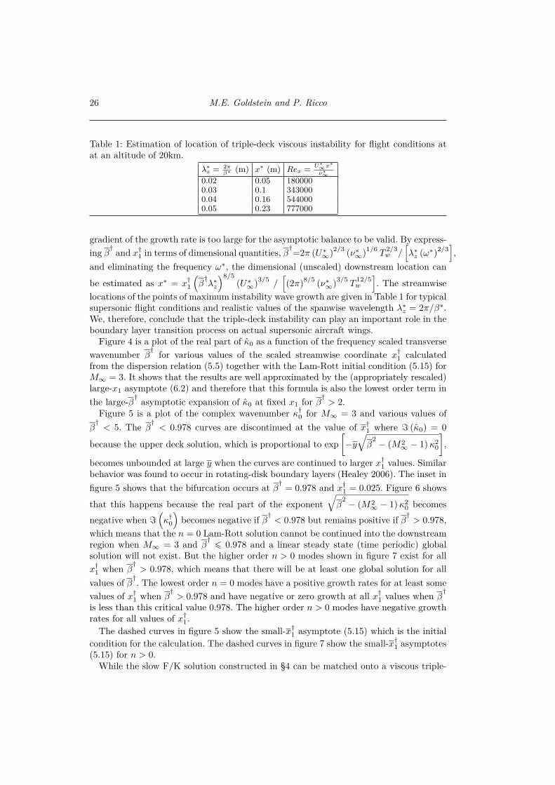
Table 1: Estimation of location of triple-deck viscous instability for flight conditions atat an altitude of 20km.
λ∗z = 2π
β∗ (m) x∗ (m) Rex =U∗
∞x∗
ν∗∞
0.02 0.05 1800000.03 0.1 3430000.04 0.16 5440000.05 0.23 777000
gradient of the growth rate is too large for the asymptotic balance to be valid. By express-
ing β†
and x†1 in terms of dimensional quantities, β
†=2π (U∗
∞)2/3
(ν∗∞)
1/6T
2/3w /
[λ∗
z (ω∗)2/3],
and eliminating the frequency ω∗, the dimensional (unscaled) downstream location can
be estimated as x∗ = x†1
(β
†λ∗
z
)8/5
(U∗∞)
3/5/[(2π)
8/5(ν∗
∞)3/5
T12/5w
]. The streamwise
locations of the points of maximum instability wave growth are given in Table 1 for typicalsupersonic flight conditions and realistic values of the spanwise wavelength λ∗
z = 2π/β∗.We, therefore, conclude that the triple-deck instability can play an important role in theboundary layer transition process on actual supersonic aircraft wings.
Figure 4 is a plot of the real part of κ0 as a function of the frequency scaled transverse
wavenumber β†
for various values of the scaled streamwise coordinate x†1 calculated
from the dispersion relation (5.5) together with the Lam-Rott initial condition (5.15) forM∞ = 3. It shows that the results are well approximated by the (appropriately rescaled)large-x1 asymptote (6.2) and therefore that this formula is also the lowest order term in
the large-β†
asymptotic expansion of κ0 at fixed x1 for β†
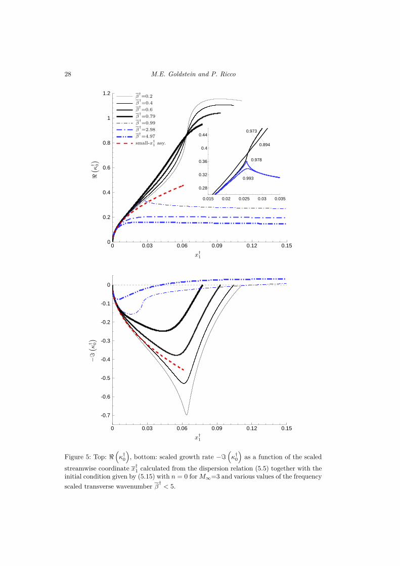
> 2.Figure 5 is a plot of the complex wavenumber κ†
0 for M∞ = 3 and various values of
β†
< 5. The β†
< 0.978 curves are discontinued at the value of x†1 where ℑ (κ0) = 0
because the upper deck solution, which is proportional to exp
[−y
√β
2 − (M2∞ − 1) κ2
0
],
becomes unbounded at large y when the curves are continued to larger x†1 values. Similar
behavior was found to occur in rotating-disk boundary layers (Healey 2006). The inset in
figure 5 shows that the bifurcation occurs at β†
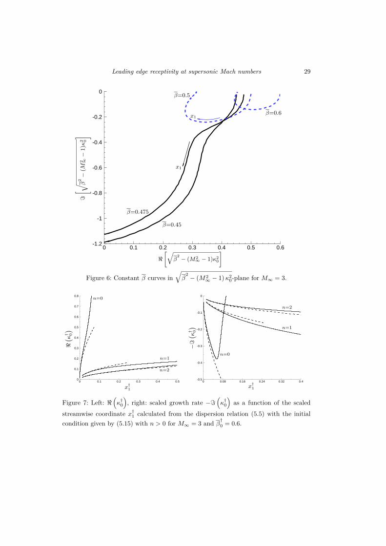
= 0.978 and x†1 = 0.025. Figure 6 shows
that this happens because the real part of the exponent
√β
2 − (M2∞ − 1) κ2
0 becomes
negative when ℑ(
κ†0
)becomes negative if β
†< 0.978 but remains positive if β
†> 0.978,
which means that the n = 0 Lam-Rott solution cannot be continued into the downstreamregion when M∞ = 3 and β
†6 0.978 and a linear steady state (time periodic) global
solution will not exist. But the higher order n > 0 modes shown in figure 7 exist for all
x†1 when β
†> 0.978, which means that there will be at least one global solution for all
values of β†. The lowest order n = 0 modes have a positive growth rates for at least some
values of x†1 when β
†> 0.978 and have negative or zero growth at all x†
1 values when β†
is less than this critical value 0.978. The higher order n > 0 modes have negative growthrates for all values of x†
1.
The dashed curves in figure 5 show the small-x†1 asymptote (5.15) which is the initial
condition for the calculation. The dashed curves in figure 7 show the small-x†1 asymptotes
(5.15) for n > 0.While the slow F/K solution constructed in §4 can be matched onto a viscous triple-

Leading edge receptivity at supersonic Mach numbers 27
1 2 3 4 5 6 7 80
0.04
0.08
0.12
0.16
0.2
0.24
0.28x†
1=0.496
x†1=1.984
x†1=9.922
β†
ℜ( κ
† 0
)
Figure 4: ℜ(
κ†0
)as a function of the frequency scaled transverse wavenumber β
†for three
values of the scaled streamwise coordinate x†1 calculated from the dispersion relation (5.5)
together with the Lam-Rott initial condition (5.15) for M∞=3. The dashed curve is the
rescaled large-x†1 asymptote (6.5), which shows that this result is also valid when β → ∞
and x†1=O(1).
deck solution when β ≡ ǫ/∆θ = O(1), we have shown (after equation (5.21)) that thisresult is unphysical because it does not remain bounded at large wall normal distancesfrom the plate. This means that a global triple-deck solution can only exist at larger ∆θ,which corresponds to the scaling
β =ǫ1−r
∆θ= O(1) (8.2)
with 0<r<1. But §5 shows that the resulting solution can only be matched onto theslow F/K solution when 1/3 6 r < 1, which means that the F/K solution cannot becontinued into the downstream region when 0 6 r < 1/3. The minimum ∆θ, which is
determined by β = ǫ2/3/∆θ = O(1) in (8.2), corresponds to an upstream diffractionregion solution that matches onto an inviscid triple-deck solution in the downstreamregion where x1 = x1ǫ4/3 = O(1), which is still further downstream than the viscoustriple-deck region where x1 = O(1) but upstream of the full Rayleigh equation regionwhere the ∆θ = O(1) solution becomes unstable.
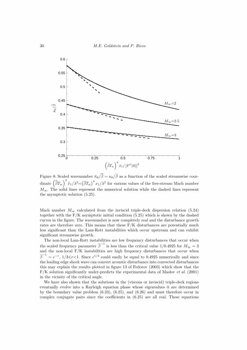
Figure 8 is a plot of the scaled wavenumber κ0/β = κ0/β as a function of the scaled
streamwise coordinate(
βTw
)4
x1/λ2=(βTw
)4x1/λ2 for various values of the free-stream
28 M.E. Goldstein and P. Ricco
0 0.03 0.06 0.09 0.12 0.150
0.2
0.4
0.6
0.8
1
1.2
0.015 0.02 0.025 0.03 0.035
0.28
0.32
0.36
0.4
0.440.973
0.894
0.978
0.993
β†=0.2
β†=0.4
β†=0.6
β†=0.79
β†=0.99
β†=2.98
β†=4.97
small-x†1 asy.
ℜ( κ
† 0
)
x†1
0 0.03 0.06 0.09 0.12 0.15
-0.7
-0.6
-0.5
-0.4
-0.3
-0.2
-0.1
0
−ℑ( κ
† 0
)
x†1
Figure 5: Top: ℜ(
κ†0
), bottom: scaled growth rate −ℑ
(κ†
0
)as a function of the scaled
streamwise coordinate x†1 calculated from the dispersion relation (5.5) together with the
initial condition given by (5.15) with n = 0 for M∞=3 and various values of the frequency
scaled transverse wavenumber β†
< 5.
Leading edge receptivity at supersonic Mach numbers 29
0 0.1 0.2 0.3 0.4 0.5 0.6-1.2
-1
-0.8
-0.6
-0.4
-0.2
0
β=0.45
β=0.475
β=0.5
β=0.6
ℜ
[√β
2− (M2
∞ − 1)κ20
]
ℑ
[ √β
2−
(M2 ∞
−1)κ
2 0
]
x1
x1
Figure 6: Constant β curves in
√β
2 − (M2∞ − 1) κ2
0-plane for M∞ = 3.
0 0.1 0.2 0.3 0.4 0.50
0.1
0.2
0.3
0.4
0.5
0.6
0.7
0.8n=0
n=1
n=2
ℜ( κ
† 0
)
x†1
0 0.08 0.16 0.24 0.32 0.4-0.5
-0.4
-0.3
-0.2
-0.1
0
n=0
n=1
n=2
−ℑ( κ
† 0
)
x†1
Figure 7: Left: ℜ(
κ†0
), right: scaled growth rate −ℑ
(κ†
0
)as a function of the scaled
streamwise coordinate x†1 calculated from the dispersion relation (5.5) with the initial
condition given by (5.15) with n > 0 for M∞ = 3 and β†
0 = 0.6.
30 M.E. Goldstein and P. Ricco
0 0.25 0.5 0.75 10.25
0.3
0.35
0.4
0.45
0.5
0.55
0.6
M∞=2
M∞=2.5
M∞=3
κ0/
¯ β
(¯βTw
)4
x1/ [F ′′(0)]2
Figure 8: Scaled wavenumber κ0/β = κ0/β as a function of the scaled streamwise coor-
dinate(
βTw
)4
x1/λ2=(βTw
)4x1/λ2 for various values of the free-stream Mach number
M∞. The solid lines represent the numerical solution while the dashed lines representthe asymptotic solution (5.25).
Mach number M∞ calculated from the inviscid triple-deck dispersion relation (5.24)together with the F/K asymptotic initial condition (5.25) which is shown by the dashedcurves in the figure. The wavenumber is now completely real and the disturbance growthrates are therefore zero. This means that these F/K disturbances are potentially muchless significant than the Lam-Rott instabilities which occur upstream and can exhibitsignificant streamwise growth.
The non-local Lam-Rott instabilities are low frequency disturbances that occur when
the scaled frequency parameter β−1
is less than the critical value 1/0.4925 for M∞ = 3and the non-local F/K instabilities are high frequency disturbances that occur when
β−1
= ǫ−r, 1/36r<1. Since ǫ1/3 could easily be equal to 0.4925 numerically and sincethe leading edge shock wave can convert acoustic disturbance into convected disturbancesthis may explain the results plotted in figure 13 of Fedorov (2003) which show that theF/K solution significantly under-predicts the experimental data of Maslov et al. (2001)in the vicinity of the critical angle.
We have also shown that the solutions in the (viscous or inviscid) triple-deck regionseventually evolve into a Rayleigh equation phase whose eigenvalues α are determinedby the boundary value problem (6.23), (6.25), and (6.26) and must therefore occur incomplex conjugate pairs since the coefficients in (6.25) are all real. These equations
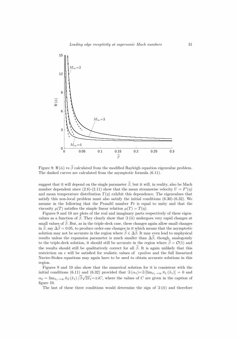
Leading edge receptivity at supersonic Mach numbers 31
0.01 0.02 0.03
10
20
0 0.05 0.1 0.15 0.2 0.25 0.30
3
6
9
12
15
M∞=2
M∞=3
M∞=4
β
ℜ(α
)
Figure 9: ℜ (α) vs β calculated from the modified Rayleigh equation eigenvalue problem.The dashed curves are calculated from the asymptotic formula (6.11).
suggest that α will depend on the single parameter β, but it will, in reality, also be Machnumber dependent since (2.8)-(2.11) show that the mean streamwise velocity U = F ′(η)and mean temperature distribution T (η) exhibit this dependence. The eigenvalues thatsatisfy this non-local problem must also satisfy the initial conditions (6.30)-(6.32). Weassume in the following that the Prandtl number Pr is equal to unity and that theviscosity µ(T ) satisfies the simple linear relation µ(T ) = T (η).
Figures 9 and 10 are plots of the real and imaginary parts respectively of these eigen-values as a function of β. They clearly show that ℑ (α) undergoes very rapid changes at
small values of β. But, as in the triple-deck case, these changes again allow small changesin β, say ∆β = 0.05, to produce order-one changes in α which means that the asymptoticsolution may not be accurate in the region where β ∈ ∆β. It may even lead to unphysicalresults unless the expansion parameter is much smaller than ∆β, though, analogouslyto the triple-deck solution, it should still be accurate in the region where β = O(1) and
the results should still be qualitatively correct for all β. It is again unlikely that thisrestriction on ǫ will be satisfied for realistic values of epsilon and the full linearizedNavier-Stokes equations may again have to be used to obtain accurate solutions in thisregion.
Figures 9 and 10 also show that the numerical solution for α is consistent with theinitial conditions (6.11) and (6.32) provided that ℑ (α1)=ℑ [limx1→∞ κ1 (x1)] = 0 and
α2 = limx1→∞ κ2 (x1) /β√
2x1=±iC, where the values of C are given in the caption offigure 10.
The last of these three conditions would determine the sign of ℑ (α) and therefore
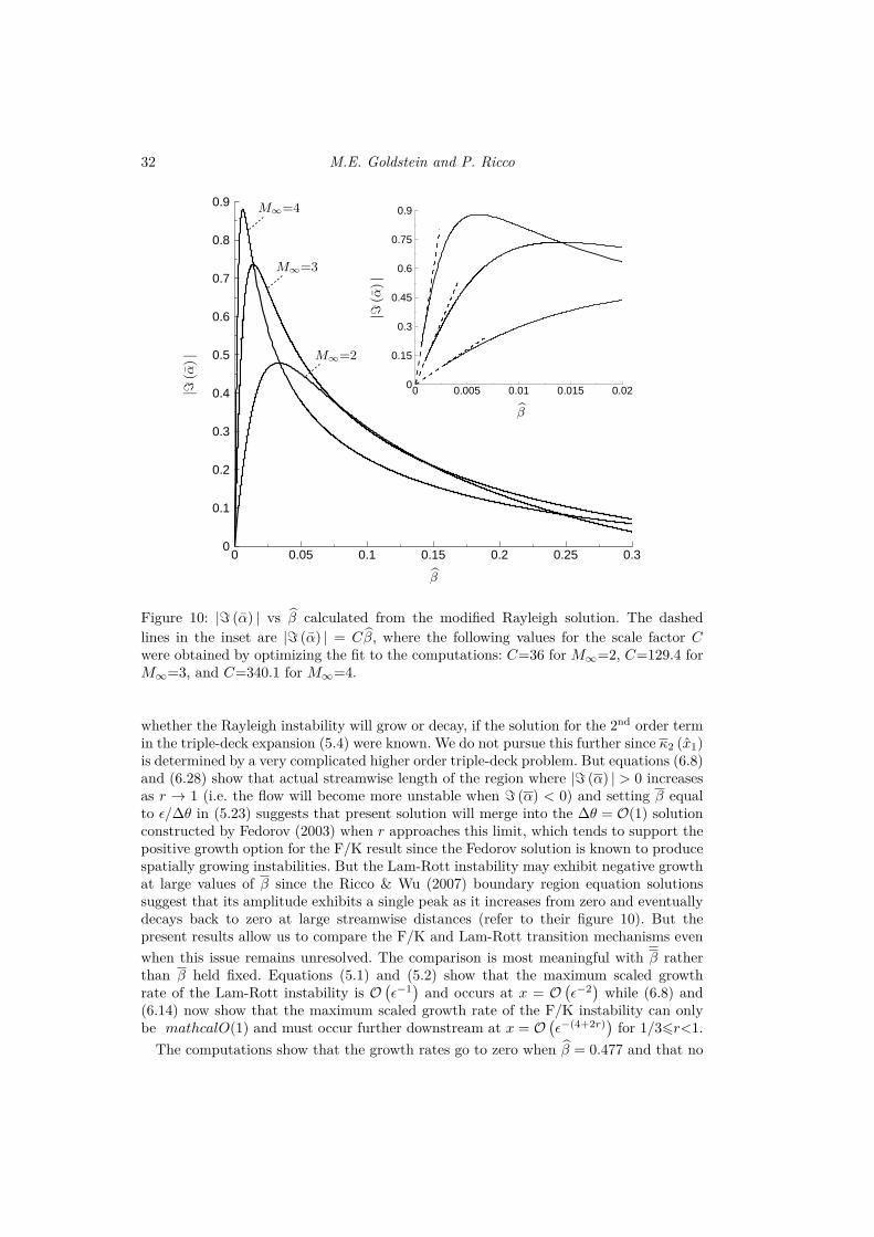
32 M.E. Goldstein and P. Ricco
0 0.05 0.1 0.15 0.2 0.25 0.30
0.1
0.2
0.3
0.4
0.5
0.6
0.7
0.8
0.9
0 0.005 0.01 0.015 0.020
0.15
0.3
0.45
0.6
0.75
0.9
M∞=2
M∞=3
M∞=4
β
β
|ℑ(α
)|
|ℑ(α
)|
Figure 10: |ℑ (α) | vs β calculated from the modified Rayleigh solution. The dashed
lines in the inset are |ℑ (α) | = Cβ, where the following values for the scale factor Cwere obtained by optimizing the fit to the computations: C=36 for M∞=2, C=129.4 forM∞=3, and C=340.1 for M∞=4.
whether the Rayleigh instability will grow or decay, if the solution for the 2nd order termin the triple-deck expansion (5.4) were known. We do not pursue this further since κ2 (x1)is determined by a very complicated higher order triple-deck problem. But equations (6.8)and (6.28) show that actual streamwise length of the region where |ℑ (α) | > 0 increasesas r → 1 (i.e. the flow will become more unstable when ℑ (α) < 0) and setting β equalto ǫ/∆θ in (5.23) suggests that present solution will merge into the ∆θ = O(1) solutionconstructed by Fedorov (2003) when r approaches this limit, which tends to support thepositive growth option for the F/K result since the Fedorov solution is known to producespatially growing instabilities. But the Lam-Rott instability may exhibit negative growthat large values of β since the Ricco & Wu (2007) boundary region equation solutionssuggest that its amplitude exhibits a single peak as it increases from zero and eventuallydecays back to zero at large streamwise distances (refer to their figure 10). But thepresent results allow us to compare the F/K and Lam-Rott transition mechanisms even
when this issue remains unresolved. The comparison is most meaningful with β ratherthan β held fixed. Equations (5.1) and (5.2) show that the maximum scaled growthrate of the Lam-Rott instability is O
(ǫ−1)
and occurs at x = O(ǫ−2)
while (6.8) and(6.14) now show that the maximum scaled growth rate of the F/K instability can onlybe mathcalO(1) and must occur further downstream at x = O
(ǫ−(4+2r)
)for 1/36r<1.
The computations show that the growth rates go to zero when β = 0.477 and that no

Leading edge receptivity at supersonic Mach numbers 33
solutions, other than the trivial solution
{u, v, w, p} = {0, 0, 0, 0}, (8.3)
exist beyond this point, which might suggest that there are no global solutions to thereceptivity problem. But equation (6.25) has a critical layer at the point where U(η) =α−1 when α is real. The Rayleigh equation solution will be regular (i.e. analytic) there
since this point coincides with the generalized inflection point where(U ′/T 2
)′= 0. But
viscous effects must be taken into account within a thin critical layer surrounding thispoint before continuing the solution into the downstream region because the streamwiseand spanwise velocity perturbations still become singular there.
The viscous effects actually come into play in a thin critical layer at the point, say xc,where ℑ (α)=O
(ǫ4/3
)which lies slightly upstream of the neutral stability point xn.s..
The difference between the corresponding scaled streamwise coordinates, say x1c − xn.s.,will also be O
(ǫ4/3
)at this point, but its actual location can otherwise be arbitrarily
specified. The critical layer flow can only be balanced by allowing the unsteady flow toevolve on the relatively fast streamwise length scale
x1 ≡ ǫ4/3 (x − xc) (8.4)
which can be done by changing the amplitude function in (6.14) and using (6.16) to showthat the streamwise velocity outside of the critical layer should expand like
u =U(η) + δ
{A(x1
)v(η; x1c)U ′(η)
iT (η)√
2x1c [1 − αcU(η)]+ ǫ4/3u1
(η, x1
)+ ...
}
× exp
{i
[1
ǫ4+2r
∫ x1
0
α (x1, ǫ) dx1 + β z − t
]},
(8.5)
where x1c denotes the scaled streamwise coordinate x1 at the location of the critical point
αc = αR + iǫ4/3κ ≡ α (x1c) (8.6)
and v (η; x1) denotes the solution to the Rayleigh equation (6.25) described in §6. Thesecond order solution can be determined from (6.15)-(6.18) with α replaced by the oper-ator αc +ǫ4/3∂/∂x1 but the O
(ǫ2(1−r)
)terms have to be included when 1/36r61, which
is the range of r-values associated with the F/K solutions.
Since (6.8) and (8.4) show that x1 ≡ ǫ4/3 (x1 − x1c) /ǫ4+2r and since x1c − x1n.s. mustbe O
(ǫ4/3
)the relatively short streamwise distance x1 can be as large as ǫ−(2r+4/3) and
still lie in the upstream region where the Rayleigh problem can be solved, which meansthat the limit x1 → ∞ will also lie in this region in a strict asymptotic sense. The outersolution (8.5) will therefore still exist and be compatible with the trivial solution (8.3)if the, as yet undetermined, amplitude function A
(x1
)goes to zero as x1 → ∞. But it
now has a singularity at the critical point which must be eliminated by accounting forviscous effects.
Balancing the viscous and convective terms shows that the streamwise velocity withinthe critical layer should expand like
u = Uc+δ{
ǫ−4/3u0
(η, x1
)+ u1
(η, x1
)+ ...
}exp
{i
[1
ǫ4+2r
∫ x1
0
α (x1, ǫ) dx1 + β z − t
]},
(8.7)
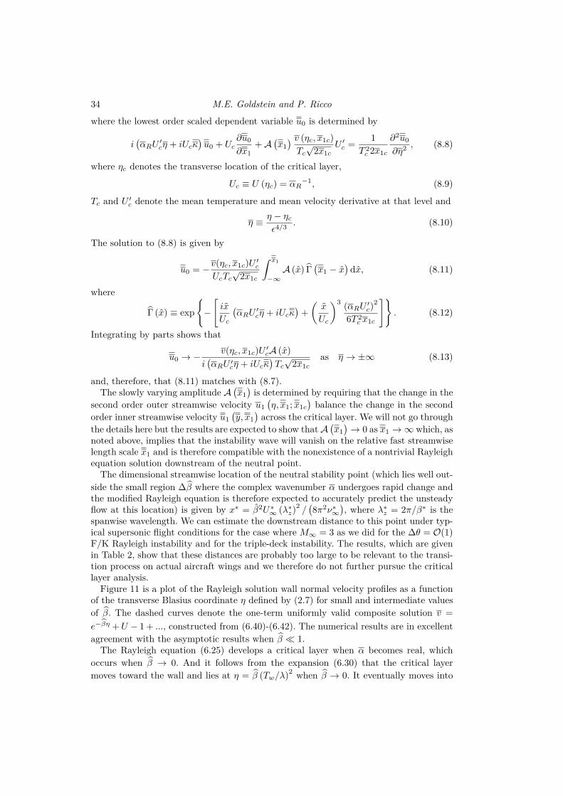
34 M.E. Goldstein and P. Ricco
where the lowest order scaled dependent variable u0 is determined by
i(αRU ′
cη + iUcκ)
u0 + Uc∂u0
∂x1+ A
(x1
) v (ηc, x1c)
Tc
√2x1c
U ′c =
1
T 2c 2x1c
∂2u0
∂η2 , (8.8)
where ηc denotes the transverse location of the critical layer,
Uc ≡ U (ηc) = αR−1, (8.9)
Tc and U ′c denote the mean temperature and mean velocity derivative at that level and
η ≡ η − ηc
ǫ4/3. (8.10)
The solution to (8.8) is given by
u0 = −v(ηc, x1c)U ′c
UcTc
√2x1c
∫ x1
−∞
A (x) Γ(x1 − x
)dx, (8.11)
where
Γ (x) ≡ exp
{−[
ix
Uc
(αRU ′
cη + iUcκ)
+
(x
Uc
)3(αRU ′
c)2
6T 2c x1c
]}. (8.12)
Integrating by parts shows that
u0 → − v(ηc, x1c)U ′cA (x)
i(αRU ′
cη + iUcκ)
Tc
√2x1c
as η → ±∞ (8.13)
and, therefore, that (8.11) matches with (8.7).The slowly varying amplitude A
(x1
)is determined by requiring that the change in the
second order outer streamwise velocity u1
(η, x1; x1c
)balance the change in the second
order inner streamwise velocity u1
(y, x1
)across the critical layer. We will not go through
the details here but the results are expected to show that A(x1
)→ 0 as x1 → ∞ which, as
noted above, implies that the instability wave will vanish on the relative fast streamwiselength scale x1 and is therefore compatible with the nonexistence of a nontrivial Rayleighequation solution downstream of the neutral point.
The dimensional streamwise location of the neutral stability point (which lies well out-
side the small region ∆β where the complex wavenumber α undergoes rapid change andthe modified Rayleigh equation is therefore expected to accurately predict the unsteadyflow at this location) is given by x∗ = β2U∗
∞ (λ∗z)
2/(8π2ν∗
∞
), where λ∗
z = 2π/β∗ is thespanwise wavelength. We can estimate the downstream distance to this point under typ-ical supersonic flight conditions for the case where M∞ = 3 as we did for the ∆θ = O(1)F/K Rayleigh instability and for the triple-deck instability. The results, which are givenin Table 2, show that these distances are probably too large to be relevant to the transi-tion process on actual aircraft wings and we therefore do not further pursue the criticallayer analysis.
Figure 11 is a plot of the Rayleigh solution wall normal velocity profiles as a functionof the transverse Blasius coordinate η defined by (2.7) for small and intermediate values
of β. The dashed curves denote the one-term uniformly valid composite solution v =
e−βη + U − 1 + ..., constructed from (6.40)-(6.42). The numerical results are in excellent
agreement with the asymptotic results when β ≪ 1.The Rayleigh equation (6.25) develops a critical layer when α becomes real, which
occurs when β → 0. And it follows from the expansion (6.30) that the critical layer
moves toward the wall and lies at η = β (Tw/λ)2
when β → 0. It eventually moves into
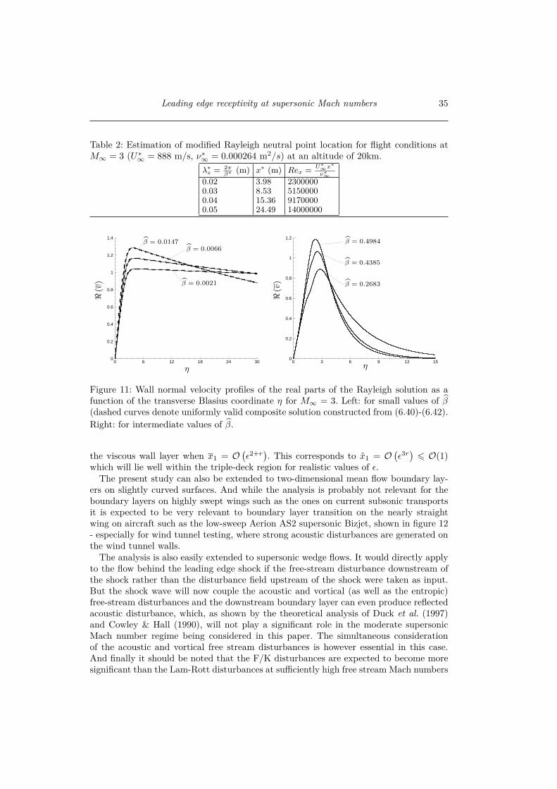
Leading edge receptivity at supersonic Mach numbers 35
Table 2: Estimation of modified Rayleigh neutral point location for flight conditions atM∞ = 3 (U∗
∞ = 888 m/s, ν∗∞ = 0.000264 m2/s) at an altitude of 20km.
λ∗z = 2π
β∗ (m) x∗ (m) Rex =U∗
∞x∗
ν∗∞
0.02 3.98 23000000.03 8.53 51500000.04 15.36 91700000.05 24.49 14000000
0 6 12 18 24 300
0.2
0.4
0.6
0.8
1
1.2
1.4
η
ℜ(v
) β = 0.0021
β = 0.0066β = 0.0147
0 3 6 9 12 150
0.2
0.4
0.6
0.8
1
1.2
η
ℜ(v
) β = 0.2683
β = 0.4385
β = 0.4984
Figure 11: Wall normal velocity profiles of the real parts of the Rayleigh solution as afunction of the transverse Blasius coordinate η for M∞ = 3. Left: for small values of β(dashed curves denote uniformly valid composite solution constructed from (6.40)-(6.42).
Right: for intermediate values of β.
the viscous wall layer when x1 = O(ǫ2+r
). This corresponds to x1 = O
(ǫ3r)6 O(1)
which will lie well within the triple-deck region for realistic values of ǫ.The present study can also be extended to two-dimensional mean flow boundary lay-
ers on slightly curved surfaces. And while the analysis is probably not relevant for theboundary layers on highly swept wings such as the ones on current subsonic transportsit is expected to be very relevant to boundary layer transition on the nearly straightwing on aircraft such as the low-sweep Aerion AS2 supersonic Bizjet, shown in figure 12- especially for wind tunnel testing, where strong acoustic disturbances are generated onthe wind tunnel walls.
The analysis is also easily extended to supersonic wedge flows. It would directly applyto the flow behind the leading edge shock if the free-stream disturbance downstream ofthe shock rather than the disturbance field upstream of the shock were taken as input.But the shock wave will now couple the acoustic and vortical (as well as the entropic)free-stream disturbances and the downstream boundary layer can even produce reflectedacoustic disturbance, which, as shown by the theoretical analysis of Duck et al. (1997)and Cowley & Hall (1990), will not play a significant role in the moderate supersonicMach number regime being considered in this paper. The simultaneous considerationof the acoustic and vortical free stream disturbances is however essential in this case.And finally it should be noted that the F/K disturbances are expected to become moresignificant than the Lam-Rott disturbances at sufficiently high free stream Mach numbers
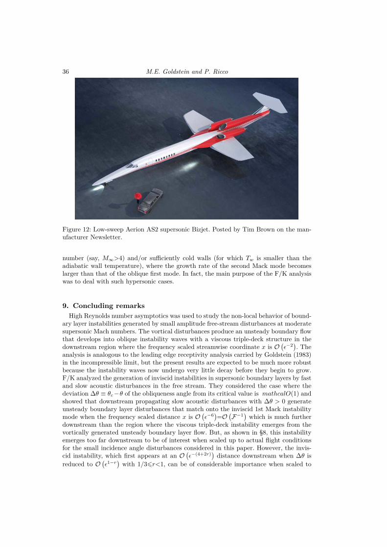
36 M.E. Goldstein and P. Ricco
Figure 12: Low-sweep Aerion AS2 supersonic Bizjet. Posted by Tim Brown on the man-ufacturer Newsletter.
number (say, M∞>4) and/or sufficiently cold walls (for which Tw is smaller than theadiabatic wall temperature), where the growth rate of the second Mack mode becomeslarger than that of the oblique first mode. In fact, the main purpose of the F/K analysiswas to deal with such hypersonic cases.
9. Concluding remarks
High Reynolds number asymptotics was used to study the non-local behavior of bound-ary layer instabilities generated by small amplitude free-stream disturbances at moderatesupersonic Mach numbers. The vortical disturbances produce an unsteady boundary flowthat develops into oblique instability waves with a viscous triple-deck structure in thedownstream region where the frequency scaled streamwise coordinate x is O
(ǫ−2). The
analysis is analogous to the leading edge receptivity analysis carried by Goldstein (1983)in the incompressible limit, but the present results are expected to be much more robustbecause the instability waves now undergo very little decay before they begin to grow.F/K analyzed the generation of inviscid instabilities in supersonic boundary layers by fastand slow acoustic disturbances in the free stream. They considered the case where thedeviation ∆θ ≡ θc −θ of the obliqueness angle from its critical value is mathcalO(1) andshowed that downstream propagating slow acoustic disturbances with ∆θ > 0 generateunsteady boundary layer disturbances that match onto the inviscid 1st Mack instabilitymode when the frequency scaled distance x is O
(ǫ−6)=O
(F−1
)which is much further
downstream than the region where the viscous triple-deck instability emerges from thevortically generated unsteady boundary layer flow. But, as shown in §8, this instabilityemerges too far downstream to be of interest when scaled up to actual flight conditionsfor the small incidence angle disturbances considered in this paper. However, the invis-cid instability, which first appears at an O
(ǫ−(4+2r)
)distance downstream when ∆θ is
reduced to O(ǫ1−r
)with 1/36r<1, can be of considerable importance when scaled to
Leading edge receptivity at supersonic Mach numbers 37
flight conditions. It is therefore appropriate to compare the vortically-generated instabil-ities with the instabilities generated by oblique acoustic disturbances with obliquenessangles in this range as is done in this paper. These acoustic disturbances generate slowboundary layer disturbances which eventually develop into oblique stable disturbanceswith inviscid triple-deck structure in a region that lies downstream of the viscous triple-deck region. The acoustically generated oblique F/K disturbances are therefore likelyto be insignificant compared to the vortically-generated Lam-Rott instabilities. The pa-per shows that both of these instabilities eventually develop into modified Rayleigh-typeinstabilities (which can either grow or decay) further downstream.
The global Lam-Rott instabilities are low frequency disturbances that occur when the
scaled frequency parameter 1/β†
is less than the critical value 1/0.978 and the global F/Kinstabilities are high frequency disturbances that occur when 1/β = 1/ǫr, 1/3 6 r < 1.Since ǫ1/3 could easily be equal to 0.978 numerically and since the leading edge shockwave can convert acoustic disturbance into convected disturbances this may explain theresults given in Fedorov (2003) which show that the F/K solution significantly under-predicts the experimental data of Maslov et al. (2001) in the vicinity of the critical angle.
This research was sponsored by NASA’s Transformational Tools and Technologies(TTT) Project of the Transformative Aeronautics Concepts Program under the Aero-nautics Research Mission Directorate. PR acknowledges the financial support by the AirForce Office of Scientific Research award number AFOSR Grant FA9550-15-1-0248. Theauthors would also like to thank Dr. Meelan Choudhari for making them aware of thephotograph in figure 12.
Appendix A. Rescaling of F/K solution for ∆θ ≪ 1
Inserting
˜x2 ≡ x2
(∆θ)a
(∆ϕ)a1
= O(1) (A 1)
and
˜y2 ≡ y2
(∆θ)b
(∆ϕ)b1
= O(1), k ≡ k∆ϕ (A 2)
into (4.12)-(4.15) yields
1
(∆θ)2b
(∆ϕ)2b1
∂2p2
∂ ˜y22
=2iα
(M2
∞ − 1)
(∆ϕ)a1 (∆θ)
a+1
∂p2
∂ ˜x2, (A 3)
1
(∆ϕ)b1 (∆θ)
b−1
∂p2
∂ ˜y2
= −iαv1(∞), p2 = p1(x2) at y2 = 0, (A 4)
v1(∞) =iαk (∆θ)
a/2(∆ϕ)
a1/2
∆ϕ∆θ cos2 θ
(√2˜x2
αλ
)2/3√˜x2p2. (A 5)
These equations will therefore remain unchanged if we put
2b = a + 1, 2b1 = a1, b1 = 1 − a1/2, b − 1 = 1 − a/2 (A 6)
and it follows that
a =3
2, b =
5
4, b1 =
1
2, a1 = 1 (A 7)
and therefore that ˜x2 and ˜y2 are given by (4.28).
38 M.E. Goldstein and P. Ricco
Appendix B. Solution for the ∆θ = O
(ǫ2/3
)viscous wall layer
The solution in the main boundary layer is given by (4.22) and (4.26). The solution inwall layer where
η ≡ η
∆ϕ=
y
ǫ3∆ϕTw
√2x
=y
Twǫ15/8 (∆θ)27/16
√2˜x2
= O(1), (B 1)
Y ≡ y
ǫ3[∆θ/ǫ2/3
]27/16(B 2)
expands like
{u, v, w, p} =∆θλη
Tw
√2˜x2
+δ
∆θ
U
(˜x2, η
),
[ǫ3
(∆θ)1/2
]7/8
V(˜x2, η
), W
(˜x2, η
),
∆θ p1
(˜x2
)}ei(αx+βz−t).
(B 3)
Inserting (B 3) along with (4.19) into the Navier-Stokes equations shows that U(˜x2, η
),
V(˜x2, η
), W
(˜x2, η
)satisfy
iαU +∂V
∂Y+ iβ W = 0, (B 4)
−i
(1 − α
λY
Tw
√2˜x2
)U +
λ
Tw
√2˜x2
V = −iαTwp1 + µwTw∂2U
∂Y 2, (B 5)
−i
(1 − α
λY
Tw
√2˜x2
)W = −iβTwp1 + µwTw
∂2W
∂Y 2, (B 6)
subject to the boundary conditions
U → −λA
Tw+
T 2w
√2˜x2β2p1
α2λY, W → − βp1T 2
w
√2˜x2
αλYas Y → ∞, (B 7)
U(0), V (0), W (0) = 0 (B 8)
which upon introducing the variable
ξ ≡ ξ0 + ξ (B 9)
where
ξ ≡ Y
(iλαTw
µw
√2˜x2
)1/3
(B 10)
and
ξ0 = −i1/3
(√2˜x2
αλ
)2/3(Tw
µw
)1/3
(B 11)
becomes
ξW = βTwξ0p1 +∂2W
∂ξ2, (B 12)
ξ∂U
∂ξ=
β
αW +
∂3U
∂ξ3, (B 13)

Leading edge receptivity at supersonic Mach numbers 39
U = 0, W = 0,∂2U
∂ξ2= −αTwξ0p1 at ξ = ξ0. (B 14)
The solution to this problem, which is now pretty standard, is
W = −πβTwξ0p1Gi (ξ0)
[Ai (ξ)
Ai (ξ0)− Gi (ξ)
Gi (ξ0)
], (B 15)
U =πβ2Twξ0p1
αGi (ξ0)
[Ai (ξ)
Ai (ξ0)− Gi (ξ)
Gi (ξ0)
]− p1Tw
(α2 + β2
)ξ0
αAi′(ξ0)
∫ ξ
ξ0
Ai (q) dq, (B 16)
where Ai and Gi denote the Airy function and Airy function integral defined on pp. 446and 448 of Abramowitz & Stegun (1964).
Matching with (4.22) and (4.23) shows that
Aλ = p1T 2w
(α2 + β2
)ξ0
αAi′(ξ0)
∫ ∞
ξ0
Ai(ξ)dξ (B 17)
and, therefore, that the wall normal velocity v(˜x2, ∞) ≡ limη→∞ v1
(˜x2, η
)is given by
(4.29).
Appendix C. Asymptotic solution to the diffraction region problem
Since the dominant contribution to the sum
ln an =n∑
j=1
lnΓ(4j/3 + 1/2)
Γ(4j/3 + 1)(C 1)
(obtained by taking the logarithm of (4.43)) comes from the terms with j > j0 where1 6 j0 6 n when n ≫ 1 it follows from equation 6.1.40 of Abramowitz & Stegun (1964)that
ln an ∼n∑
j=j0
lnΓ(4j/3 + 1/2)
Γ(4j/3 + 1)∼ −1
2
n∑
j=j0
ln
(4j
3
)∼ −1
2
∫ n
j0
ln
(4η
3
)dη
∼ −n
2
[ln
(4n
3
)− 1
] (C 2)
and, therefore, that
an ∼ A
(3e
4n
)n/2
, (C 3)
where A is a constant. Then since the main contribution to the series (4.41) comes fromits infinite tail when Z → ∞ it follows that (Bender & Orszag 1999, pp. 376-379).
p1 =
∞∑
n=0
anZn ∼ A
(2π)1/4
∞∑
n=N
(e1/2Z
)n
(4n/3)n/2
∼ A
(2π)1/4
∫ ∞
T
(Z
√3e
4t
)t
dt
∼ 3AZ2
4(2π)1/4
∫ ∞
4T/3Z2
( e
τ
)3τZ2/8
dτ ∼ 3AZ2
4(2π)1/4
∫ ∞
0
e−(3τZ2/8)(ln τ−1)dτ.
(C 4)
Then since the dominant contribution to this integral comes from the saddle point atln τ = 0, applying the method of steepest descent shows that p1 behaves like
p1 ∼ 3A
4(2π)1/4
√4π
Z2Z2e3Z2/8 =
3AZ
2
(π
2
)1/4
e3Z2/8. (C 5)

40 M.E. Goldstein and P. Ricco
Appendix D. Comparison with Ricco-Wu-2007 solution
Ricco & Wu (2007) show that
∫ ∞
ξ0
Ai(q)dq = (iα)−1/3
[F ′′(0)√
2x1
]5/3(µw
T 7w
)1/3
[1 −
(M2
∞ − 1)
(α1s)2]1/2
1 + (α1s)2 Ai′ (ξ0) ,
(D 1)
x1 =k3x
k1
√k1
R∆, ξ0 = −i1/3
[ √2x1
α1F ′′(0)
]2/3(Tw
µw
)1/3
(D 2)
and
s ≡ k5/41 R
1/4∆
k3/23
, k1 ≡ ω∗∆∗
U∗∞
, (D 3)
where ∆∗ denotes their spanwise scale factor, k3 denotes a scaled spanwise wavenumberand it follows from (2.13) and (2.14) that
R∆ ≡ U∗∞∆∗
ν∗∞
→ k1
ǫ6. (D 4)
Comparing (D 2)-(D 4) with (3.6), (4.6), and (5.12) of Ricco & Wu (2007) shows that
k3
k1→ β
ǫ, α1 →
√βκ0. (D 5)
And it, therefore, follows that
sα1 → κ0
β, x1 → βx1. (D 6)
REFERENCES
Abramowitz, M. & Stegun, I. A. 1964 Handbook of Mathematical Functions. Nat. BureauStand. Appl. Math. Ser. 55.
Bender, M. & Orszag, S. A. 1999 Advanced Mathematical Methods for Scientists and Engi-neers - Asymptotic methods and perturbation theory. Springer.
Cowley, S.J. & Hall, P. 1990 On the instability of hypersonic flow past a wedge. J. FluidMech. 214, 17–42.
Duck, P.W., Lasseigne, D.G. & Hussaini, M.Y. 1997 The effect of three-dimensionalfreestream disturbances on the supersonic flow past a wedge. Physics of Fluids 9 (2),456–467.
Fedorov, A.V. 2003 Receptivity of a high-speed boundary layer to acoustic disturbances. J.Fluid Mech. 491, 101–129.
Fedorov, A.V. & Khokhlov, A.P. 1991 Excitation of unstable modes in a supersonic bound-ary layer by acoustic waves. Fluid Dynamics 26 (4), 531–537.
Gil, A., Segura, J. & Temme, N.M. 2001 Computing complex Airy functions by numericalquadrature. Modelling, Analysis and Simulation Report MAS-R0117, November 30th, 2001- Centrum voor Wiskunde en Informatica - Amsterdam .
Glauert, M.B. 1956 The laminar boundary layer on oscillating plates and cylinders. J. FluidMech. 1, 97–110.
Goldstein, M.E. 1976 Aeroacoustics. New York, McGraw-Hill Int. Book Co., 1976. .Goldstein, M.E. 1983 The evolution of Tollmien-Schlichting waves near a leading edge. J.
Fluid Mech. 127, 59–81.Goldstein, M.E. 2003 A generalized acoustic analogy. J. Fluid Mech. 488, 315 – 333.Goldstein, M.E., Sockol, P.M. & Sanz, J. 1983 The evolution of Tollmien-Schlichting waves
near a leading edge. Part 2. Numerical determination of amplitudes. J. Fluid Mech. 129,443–453.
Leading edge receptivity at supersonic Mach numbers 41
Gulyaev, A.N., Kozlov, V.E., Kuzenetsov, V.R., Mineev, B.I. & Sekundov, A.N. 1989Interaction of a laminar boundary layer with external turbulence. Fluid Dynamics. Trans-lated from Izv, Akad. Navk. SSSR Mekh. Zhid. Gaza 6, vol. 5, pp. 55-65. 24 (5), 700–710.
Healey, J.J. 2006 A new convective instability of the rotating-disk boundary layer with growthnormal to the disk. J. Fluid Mech. 560, 279–310.
Kovasznay, L.S.G. 1953 Turbulence in supersonic flow. J. Aero. Sc. 20 (10), 657–682.Lam, S. H. & Rott, N. 1960 Theory of linearized time-dependent boundary layers. Cornell
University Grad. School of Aero. Engineering Dept. - AFOSR TN-60-1100 .Mack, L.M. 1984 Boundary-layer linear stability theory. Special Course on Stability and Tran-
sition of Laminar flow. AGARD Report 709 pp. 1–81.Maslov, A.A., Shiplyuk, A.N., Sidorenko, A.A. & Arnal, D. 2001 Leading-edge recep-
tivity of a hypersonic boundary layer on a flat plate. J. Fluid Mech. 426, 73–94.Prandtl, L. 1938 Zur berechnung der grenzschichten. ZAMM-J. Appl. Math. and Mechanic-
s/Zeitschrift fur Angewandte Mathematik und Mechanik 18 (1), 77–82.Reshotko, E. 1976 Boundary-layer stability and transition. Ann. Rev. Fluid Mech. 8 (1), 311–
349.Ricco, P. & Wu, X. 2007 Response of a compressible laminar boundary layer to free-stream
vortical disturbances. J. Fluid Mech. 587, 97–138.Smith, F.T. 1989 On the first-mode instability in subsonic, supersonic or hypersonic boundary
layers. J. Fluid Mech. 198, 127–153.Stewartson, K. 1964 The theory of laminar boundary layers in compressible fluids. Oxford,
Claredon Press.Wanderley, J.B.V. & Corke, T.C. 2001 Boundary layer receptivity to free-stream sound on
elliptic leading edges of flat plates. J. Fluid Mech. 429, 1–21.Wu, X. 1999 Generation of Tollmien-Schlichting waves by convecting gusts interacting with
sound. J. Fluid Mech. 397, 285–316.