2009 - Improving Malware Detection by Applying Multi-Inducer Ensemble (journal)
12
Computational Statistics and Data Analysis 53 (2009) 1483–1494 Contents lists available at ScienceDirect Computational Statistics and Data Analysis journal homepage: www.elsevier.com/locate/csda Improving malware detection by applying multi-inducer ensemble Eitan Menahem, Asaf Shabtai, Lior Rokach * , Yuval Elovici Duetsche Telekom Laboratories, Ben-Gurion University of the Negev, Be’er Sheva, 84105, Israel article info Article history: Received 23 July 2008 Accepted 4 October 2008 Available online 19 October 2008 abstract Detection of malicious software (malware) using machine learning methods has been explored extensively to enable fast detection of new released malware. The performance of these classifiers depends on the induction algorithms being used. In order to benefit from multiple different classifiers, and exploit their strengths we suggest using an ensemble method that will combine the results of the individual classifiers into one final result to achieve overall higher detection accuracy. In this paper we evaluate several combining methods using five different base inducers (C4.5 Decision Tree, Naïve Bayes, KNN, VFI and OneR) on five malware datasets. The main goal is to find the best combining method for the task of detecting malicious files in terms of accuracy, AUC and Execution time. © 2008 Elsevier B.V. All rights reserved. 1. Introduction Modern computer and communication infrastructure are highly susceptible to various types of attacks. A common way of launching these attacks is using malware (malicious software) such as worm, virus, Trojan or spyware (Kienzle and Elder, 2003; Heidari, 2004). A spreading malicious software might generate great damage to private users, commercial companies and governments. A single malware in a computer, which is a part of a computer network, can result in the loss, or unauthorized utilization or modification, of large amount of data and cause users to question the reliability of all of the information on the network. Detection of known malware is commonly performed by using anti-virus tools. These tools detect the known malware using signature detection methods (White, 1999; Dikinson, 2005). When a new malware is released, the anti-virus vendors need to catch an instance of the new malware, analyze it, create a new signature and update their clients. During the period between the appearance of a new unknown malware and the update of the signature-base of the anti-virus clients, millions of computers are vulnerable to the new malware. Therefore, although signature-based detection methods eventually yield high detection rate, they cannot cope with new, unseen before, malware (White, 1998). High-speed communication channels enable malware to propagate and infect hosts quickly and so it is essential to detect and eliminate new (unknown) spreading malware at early stages of the attack. Recent studies have proposed methods for detecting malicious executables using Machine Learning (ML) tech- niques (Kabiri and Ghorbani, 2005). Given a training set of malicious and benign executable binary codes, a classifier is trained to identify and classify unknown malicious executables as being malicious. Some of the methods are inspired by text categorization techniques, in which words are analogous to sequences in the binary code. Malicious and benign files are represented by a vector of features, extracted from the PE-header and the binary code of the executable. These files are used to train a classifier. During the detection phase, based on the generalization capability of the classifier, an unknown file can be classified as malicious or benign. Some of the studies applying machine learning methods on content-based features are mentioned below. * Corresponding author. E-mail addresses: [email protected] (E. Menahem), [email protected] (A. Shabtai), [email protected] (L. Rokach), [email protected] (Y. Elovici). 0167-9473/$ – see front matter © 2008 Elsevier B.V. All rights reserved. doi:10.1016/j.csda.2008.10.015
Transcript of 2009 - Improving Malware Detection by Applying Multi-Inducer Ensemble (journal)

Computational Statistics and Data Analysis 53 (2009) 1483–1494
Contents lists available at ScienceDirect
Computational Statistics and Data Analysis
journal homepage: www.elsevier.com/locate/csda
Improving malware detection by applying multi-inducer ensembleEitan Menahem, Asaf Shabtai, Lior Rokach ∗, Yuval EloviciDuetsche Telekom Laboratories, Ben-Gurion University of the Negev, Be’er Sheva, 84105, Israel
a r t i c l e i n f o
Article history:Received 23 July 2008Accepted 4 October 2008Available online 19 October 2008
a b s t r a c t
Detection of malicious software (malware) using machine learning methods has beenexplored extensively to enable fast detection of new releasedmalware. The performance ofthese classifiers depends on the induction algorithms being used. In order to benefit frommultiple different classifiers, and exploit their strengths we suggest using an ensemblemethod that will combine the results of the individual classifiers into one final result toachieve overall higher detection accuracy. In this paper we evaluate several combiningmethods using five different base inducers (C4.5 Decision Tree, Naïve Bayes, KNN, VFI andOneR) on five malware datasets. The main goal is to find the best combining method forthe task of detecting malicious files in terms of accuracy, AUC and Execution time.
© 2008 Elsevier B.V. All rights reserved.
1. Introduction
Modern computer and communication infrastructure are highly susceptible to various types of attacks. A common wayof launching these attacks is using malware (malicious software) such as worm, virus, Trojan or spyware (Kienzle andElder, 2003; Heidari, 2004). A spreading malicious software might generate great damage to private users, commercialcompanies and governments. A single malware in a computer, which is a part of a computer network, can result in theloss, or unauthorized utilization or modification, of large amount of data and cause users to question the reliability of all ofthe information on the network.Detection of known malware is commonly performed by using anti-virus tools. These tools detect the known malware
using signature detection methods (White, 1999; Dikinson, 2005). When a newmalware is released, the anti-virus vendorsneed to catch an instance of the newmalware, analyze it, create a new signature and update their clients. During the periodbetween the appearance of a new unknownmalware and the update of the signature-base of the anti-virus clients, millionsof computers are vulnerable to the new malware. Therefore, although signature-based detection methods eventually yieldhighdetection rate, they cannot copewithnew, unseenbefore,malware (White, 1998). High-speed communication channelsenablemalware to propagate and infect hosts quickly and so it is essential to detect and eliminate new (unknown) spreadingmalware at early stages of the attack.Recent studies have proposed methods for detecting malicious executables using Machine Learning (ML) tech-
niques (Kabiri and Ghorbani, 2005). Given a training set of malicious and benign executable binary codes, a classifier istrained to identify and classify unknown malicious executables as being malicious. Some of the methods are inspired bytext categorization techniques, in which words are analogous to sequences in the binary code. Malicious and benign filesare represented by a vector of features, extracted from the PE-header and the binary code of the executable. These files areused to train a classifier. During the detection phase, based on the generalization capability of the classifier, an unknown filecan be classified as malicious or benign. Some of the studies applying machine learning methods on content-based featuresare mentioned below.
∗ Corresponding author.E-mail addresses: [email protected] (E. Menahem), [email protected] (A. Shabtai), [email protected] (L. Rokach), [email protected] (Y. Elovici).
0167-9473/$ – see front matter© 2008 Elsevier B.V. All rights reserved.doi:10.1016/j.csda.2008.10.015

1484 E. Menahem et al. / Computational Statistics and Data Analysis 53 (2009) 1483–1494
In Schultz et al. (2001), ML techniques were applied for detection of unknown malicious code based on binary codecontent. Three different feature extraction methods are used: program header, printable string features and byte Sequencefeatures, on which they applied four classifiers: Signature-based method (anti-virus), Ripper — a rule-based learner, NaïveBayes and Multi-Naïve Bayes. The experiments conducted using 4301 programs in Win32 PE format (3301 maliciousprograms and 1000 benign programs) and the results show that all ML methods outperform the signature-based classifier.The study in Abou-Assaleh et al. (2004) used n-gram features extracted from the binary code of the file. The L most
frequent n-grams of each class in the training set are chosen and represent the profile of the class. A new instance isassociated to a class with the closest profile using KNN algorithm. The experiment conducted on a small set of 65 maliciousand benign files achieved 98% accuracy. Caia et al. (2007) and Moskovitch et al. (2008) have compared different featureselection methods for building a single classifier.Kolter and Maloof (2006) extracted n-grams from the executables. Most relevant n-gram attributes were chosen using
Info-Gain ratio and the datasets were evaluated using several inducers: IBK, Naïve Bayes, Support Vector Machines (SVMs),Decision Trees, Boosted Naïve Bayes, Boosted SVMs, and Boosted Decision Tree algorithms. Since costs of misclassificationerror are usually unknown, the methods were evaluated using receiver operating characteristic (ROC) analysis. Whenclassifying new instances into two optional classes ‘Benign’ and ‘Malicious’, Boosted decision trees outperformed othermethodswith an area under the ROC curve of 0.996.When classifying new instances intomulti-class (such as Virus, Backdooretc.), the area under the ROC curve reaches an average of 0.9.By its nature, the measured performance (e.g., accuracy) of a machine learning classifier is influenced by two main
factors: (1) the inducer algorithm that is used to generate the classifier (e.g., Artificial Neural Network, Decision Tree, NaïveBayes); and (2) the types of features that are used to represent the instances. Thus, various types of classifiers have different‘‘inductive biases’’. When generating multiple classifiers using different inducers and various features (that are extractedfrom the same set of instances) each classifier will perform differently. It might be the case that a certain classifier will bespecialized in classifying instances into a subset of classes (for example, a classifier that classifies an executable file as benignor Wormwith high accuracy but with low accuracy when classifying into other malicious classes such as Trojan and Virus).The outcome of this observation is that one should use multiple different classifiers that will classify a new instance
predicting its real class (like a group of experts) and then combining all the results, using an intelligent combinationmethod,into one final result. Hopefully, this ‘‘super-classifier’’ will outperform each of the individual classifiers and classify newinstances with higher accuracy by learning the strength and weakness of each classifier.In this paper we introduce three main contributions: (1) we show that multi-inducer ensembles are capable of detecting
malwares; (2) we introduce an innovative combining method, called Troika (Menahem, 2008) which extends Stacking andshows its superiority in the malware detection tasks; and (3) we present empirical results from an extensive real worldstudy of various malwares using different types of features.The rest of the paper is organized as follows. In Section 2 we describe related work in the field of ensemble application
in the security domain. Section 3 presents the experimental setup and in Section 4 we present the evaluation results.Conclusions and future work are discussed in Section 5.
2. Related work
In this sectionwe present studies inwhich ensemblemethods are used to aid inmalicious code detection and in intrusiondetection. We also describe the six ensemble methods used in our experiments.
2.1. Malware detection using ensemble methods
The main idea of an ensemble methodology is to combine a set of classifiers in order to obtain a better composite globalclassifier. Ensemble methodology imitates our second nature to seek several opinions before making any crucial decision.We weigh the individual opinions, and combine them to reach a final decision. Recent studies evaluated the improvementin performance (in terms of accuracy, false-positive rate and area under the ROC graph) when using ensemble algorithmsto combine the individual classifiers.Several researchers examined the applicability of ensemble methods in detecting malicious code. Zhang et al. (2007)
classifies new malicious code based on n-gram features extracted from binary code of the file. First, n-gram-basedfeatures are extracted and the best n-grams are chosen by applying the Information-Gain feature selection method. Then,probabilistic neural network (PNN) is used to construct several classifiers for detection. Finally, the individual decisions of thePNN classifiers are combined by using the Dempster–Shafer theory to create the combining rules. Themethodwas evaluatedon a set ofmalicious executables that were downloaded from thewebsite VXHeavens (http://www.vx.netlux.org) and cleanprograms gathered from aWindows 2000 server machine: total of 423 benign programs and 450 malicious executable files(150 Viruses, 150 Trojans and 150Worms) all in Windows PE format. The results show a better ROC curve for the ensembleof PNNs when compared to the individual best PNN of each of the three malware classes.Ensemble of classifiers was evaluated on intrusion detection tasks as well. Mukkamalaa et al. (2005) used the Majority
Voting schema to ensemble the results of multiple classifiers trained to detected intrusions within network traffic. Theperformance of the ensemble results was compared to the performance of the individual classifiers: SVM, MARS and threetypes of ANNs (RP, SCG and OSS) and it was evaluated using DARPA dataset which is considered as an IDS evaluation

E. Menahem et al. / Computational Statistics and Data Analysis 53 (2009) 1483–1494 1485
benchmark. The classifiers were trained to detect normal traffic as well as four classes of attacks (probing, DOS, user toroot and remote to user). It is shown that the simple majority voting schema improves the accuracy of the detection.The ensemble approach in Kelly et al. (2006) was evaluated using two anomaly network intrusion detection systems,
LERAD (Mahoney, 2003) and PAYL (Wang and Stolfo, 2004). LERAD’s normal behavior is composed of rule sets of expected(normal) user behavior, and PAYL uses byte distributions derived from normal packets. Based on the classification of the twosystems as produced on a training set, an ensemble probability classification matrix (EPCM) is generated using conditionalprobability. The method was evaluated on DARPA dataset and results show an increase in the rate of detecting attacks andthe accuracy in determining their exact classes.In order to make the ensemble more effective, there should be some sort of diversity between the classifiers (Kuncheva,
2005). In multi-inducer strategy, diversity is obtained by using different types of inducers. Each inducer contains an explicitor implicit bias that leads it to prefer certain generalizations over others. Ideally, this multi-inducer strategy would alwaysperform aswell as the best of its ingredients. Evenmore ambitiously, there is hope that this combination of paradigmsmightproduce synergistic effects, leading to levels of accuracy that neither atomic approach by itself would be able to achieve.In this study we compare several methods for combining various classifiers in order to understand which of these
methods (if any) best improves the detection accuracy.
2.2. Methods for combining ensemble’s members
In the Majority Voting combining scheme (Kittler et al., 1998), a classification of an unlabeled instance is performedaccording to the class that obtains the highest number of votes (the most frequent vote). This method is also known as theplurality vote (PV) or the basic ensemble method (BEM). This approach has frequently been used as a combiningmethod forcomparing to newly proposed methods. Mathematically it can be written as:
class(x) = argmaxci∈dom(y)
(∑k
g(yk(x), ci)
)(1)
where yk(x) is the classification of the kth classifier and g(y, c) is an indicator function defined as:
g(y, c) ={1, y = c0, y 6= c. (2)
Note that in the case of a probabilistic classifier, the crisp classification yk(x) is usually obtained as follows:
yk(x) = argmaxci∈dom(y)
P̂Mk(y = ci|x) (3)
whereMk denotes classifier k and P̂Mk(y = ci|x) denotes the probability of y obtaining the value c given an instance x.In Performance Weighting, the weight of each classifier is set proportional to its accuracy performance on a validation set
(Opitz and Shavlik, 1996):
αi =(1− Ei)t∑j=1(1− Ei)
(4)
where Ei is a normalization factor which is based on the performance evaluation of classifier i on a validation set.The idea of Distribution Summation combining method is to sum up the conditional probability vector obtained from
each classifier (Clark and Boswell, 1991). The selected class is chosen according to the highest value in the total vector.Mathematically, it can be written as:
Class(x) = argmaxci∈dom(y)
∑k
P̂Mk(y = ci|x). (5)
In the Bayesian Combinationmethod theweight associatedwith each classifier is the posterior probability of the classifiergiven the training set (Buntine, 1990).
Class(x) = argmaxci∈dom(y)
∑k
P(Mk|S) · P̂Mk(y = ci|x) (6)
where P(Mk|S) denotes the probability that the classifier Mk is correct given the training set S. The estimation of P(Mk|S)depends on the classifier’s representation. To estimate this value for decision trees the reader is referred to Buntine (1990).Using Bayes’ rule, one can extend the Naïve-Bayes idea for combining various classifiers (John and Langley, 1995):
Class(x) = arg maxcj∈dom(y)
P̂(y=cj)>0
P̂(y = cj) ·∏k=1
P̂Mk(y = cj|x)
P̂(y = cj). (7)

1486 E. Menahem et al. / Computational Statistics and Data Analysis 53 (2009) 1483–1494
Fig. 1. TroikaArchitecture reveals three layers of combining classifiers; the Specialist classifiers combine the outputs of the base-classifiers,Meta-classifierscombine the Specialist classifier outputs, and finally, the Super-classifier, combines all Meta-classifier outputs. The Super-classifier is responsible for theoutput of Troika’s prediction.
Stacking is a technique whose purpose is to achieve the highest generalization accuracy (Wolpert, 1992). By using ameta-learner, this method tries to induce which classifiers are reliable and which are not. Stacking is usually employedto combine models built by different inducers. The idea is to create a meta-dataset containing a tuple for each tuple inthe original dataset. However, instead of using the original input attributes, it uses the predicted classifications by theclassifiers as the input attributes. The target attribute remains as in the original training set. A test instance is first classifiedby each of the base-classifiers. These classifications are fed into a meta-level training set from which a meta-classifier isproduced.This classifier (Meta-classifier) combines the different predictions into a final one. It is recommended that the original
dataset should be partitioned into two subsets. The first subset is reserved to form the meta-dataset and the second subsetis used to build the base-level classifiers. Consequently the meta-classifier predictions reflect the true performance of base-level learning algorithms. Stacking performance can be improved by using output probabilities for every class label fromthe base-level classifiers. It has been shown that with stacking, the ensemble performs (at best) comparably to selecting thebest classifier from the ensemble by cross-validation (Dzeroski and Zenko, 2004).Troika (Menahem, 2008) was designed to address Stacking problems, namely, the poor performance on multi-class
problems (Seewald, 2003). Troika’s ensemble scheme is general purpose which may be used to combine any types ofclassifiers which were trained on any subgroup of possible classes of a problem’s domain. In other words, it is possiblewith Troika to combine models (classifiers) that were trained on, and therefore may later predict, non-congruent datasets,in terms of instance classes. Troika uses three layers of combining classifiers (Fig. 1), rather than one, as with Stacking.The result is a better ensemble scheme, usually with multi-class problems where there are enough instances (Menahem,2008). In Menahem (2008) the writer shows that Troika, on average, is better than using the best classifier selected usingcross-validation.

E. Menahem et al. / Computational Statistics and Data Analysis 53 (2009) 1483–1494 1487
3. Evaluation description
In this section we specify the conditions in which all combination methods had been tested. Our goal was to create aground onwhich all combinationmethods could be correctly compared. Firstwe indicate the algorithms compared. Thenwedescribe the training process and the datasets we had used. Next, we show themetrics we used tomeasure the performanceof the ensemble schemes, and finally, we display and review the results of the experiments in detail.
3.1. Base-classifiers and combination methods
In the experiment we had used five different inducers as our base-classifiers: C4.5 (Quinlan, 1993), KNN (Kibler, 1991),VFI (Guvenir, 1997), OneR (Holte, 1993) and Naïve Bayes (John and Langley, 1995). Each inducer belongs to different familyof classifiers. For example, C4.5 is related to Decision Trees, KNN belongs to Lazy classifiers, OneR to Rules, Naïve-Bayesto Bayes classifiers and VFI to general. We have chosen those five inducers because (1) they are from different classifierfamilies, therefore, may yield different models that eventually will classify differently on some inputs. In an ensemble, thecombination of the output of several classifiers is only useful if they disagree about some inputs (Tumer and Ghosh, 1996),and (2) there is a difference in classification accuracy among the inducers; preliminary experiments on our datasets showthat C4.5 and KNN are relatively accurate (have better than 80% accuracy) while OneR and Naïve Bayes are not. This propertymay differentiate between a good ensemble and a bad one, because we expect that a good ensemble will mostly use theinformation made by the good inducers, while ignoring most of the poor inducers.In this study, we compared the following combination methods: best classifier (classifier which outperforms all
the others, selected using cross-validation), Majority Voting, Performance Weighting, Distribution Summation, BayesianCombination, Naïve Bayes, Stacking and Troika. The examined ensemble schemes were implemented in WEKA (Witten andFrank, 2005) in the JAVA programming language.
3.2. Datasets
We collected a large set of 22,735 benign files and 7690malware that were identified asWin32 executable and DLLs. Foreach file three types of features were extracted: n-grams, Portable Executable (PE) features and Function-based features asdescribed bellow.We developed a tool that extracts n-grams from the binary representation of a file. The tool parsed the files using a sliding
window producing n-grams of varying lengths (denoted by n). We extracted vocabularies of 16,777,216, 1,084,793,035,1,575,804,954 and 1,936,342,220, for 3-gram, 4-gram, 5-gram and 6-gram respectively. Next, each n-gram term wasrepresented using its Term Frequency (TF) and its Inverse Document Frequency (TF–IDF). The TF measure is the numberof its appearances in the file, divided by the term with the maximal appearances. IDF is the log value of the number of filesin thewhole repository, divided by the number of files that includes the term. The TF–IDFmeasure is obtained bymultiplyingTF by IDF.In ML applications, the large number of features in many domains presents a huge problem in that some features might
not contribute (possibly even harm) to the classification accuracy. Moreover, in our case, trimming the number of featuresis crucial; however, this should be done without diminishing classification accuracy. The reason for this constraint is that,as shown above, the vocabulary size may exceed billions of features, far more than the processing capacity of any abundantfeature selection tool. Moreover, it is important to identify those terms that appear most frequently in files in order to avoidvectors that contain many zeros. Thus, we first extracted the top features based on the Document Frequency (DF) measure,which is the number of files the term was found in. We selected the top 0–5500 features which appear in most of thefiles, (those with highest DF scores) and the top 1000–6500 features. Finally, we used three methods of feature selection:Document Frequency, Fisher Score (Golub et al., 1999), and Gain Ratio (Mitchell, 1997) in order to choose the top 50, top100, top 200 and top 300 n-grams, out of the 5500 n-grams, to be used for the evaluation.After performing rigorous experiments in which we evaluated several inducers on the 192 different n-gram datasets,
we chose the top 300 5-grams with TF–IDF values, top 300 6-grams with TF–IDF and top 300 6-grams, with TF datasetsproviding the best results.Certain parts of EXE files might indicate that a file is affected by a virus. This may be an inconsistency between different
parts of version numbers or internal/external name of a file; some patterns in imported DLLs may be typical of a virus. Toverify our hypothesis, we statically extracted different Portable Executable (PE) format features that represented informationcontainedwithin eachWin32 PE binary (EXE orDLL). For this purpose, the tool namedPE Feature Extractorwas implementedin C++. Feature Extractor parses an EXE\DLL file according to PE Format rules. The information extracted by this tool is asfollows (total of 88 attributes):
- Information extracted from the PE-header that describes the details about physical structure of a PE binary(e.g., creation\modification time, machine type and file size)- Optional PE-header information describing the logical structure of a PE binary (e.g., linker version, section alignment,code size and debug flags)- Import Section: which DLLs were imported and which functions from the imported DLLs that were used

1488 E. Menahem et al. / Computational Statistics and Data Analysis 53 (2009) 1483–1494
Table 1Properties of the datasets we used in our experiment.
Dataset #Classes #Instances #Attributes
6-grams TF-2C 2 9914 316-grams TF–IDF-2C 2 9914 315-grams TF–IDF-2C 2 9914 31PE-2C 2 8247 30FD-2C 2 9914 176-grams TF-8C 8 9914 316-grams TF–IDF-8C 8 9914 315-grams TF–IDF-8C 8 9914 31PE-8C 2 8247 30FD-8C 2 9914 17
- Export Section: which functions were exported (if the file being examined is a DLL)- Resource Directory: resources used by a given file (e.g., dialogs and cursors)- Version Information: (e.g., internal and external name of a file, version number).
A new method for extracting features from the binary code of the files was implemented and extracted for theexperiment. In this method (hereby Function Detector method) we use a J48 decision tree classifier in order to mark thebeginning and ending of functions residing in the binary representation of the files. Using those marks we extract thefunction from each file and generate the following attributes (total of 17 attributes):
- Size of file- File’s entropy value- Total number of detected functions- Size of the longest function that was detected- Size of the shortest function that was detected- Average size of detected functions- Standard deviation of the size of detected functions- Number of functions divided into fuzzy groups by its length in bytes (16, 24, 40, 64, 90, 128 and 256 bytes)- Function ratio — the proportion of number of detected functions from the overall size of the file- Code ratio — the proportion of the size (in bytes) of detected functions from the overall size of the file.
Unfortunately, due to processing power and memory limitations we could not run our ensemble experiments on theentire datasets and we had to reduce the datasets in order to complete the experiments in reasonable time.Therefore, for the evaluation process we had produced a new dataset from the original dataset by choosing randomly
33% of the instances (i.e., files) in the original datasets and we applied the Gain Ratio feature selection method (Mitchell,1997) on the n-gram-based and PE datasets.As a result, each ensemble scheme in our experiment was tested upon 10 datasets. Table 1 shows the properties of the
datasets we had used in our experiment. We had 5 different datasets, and each dataset had two versions. The first versioncontained binary classification (each instance has a ‘benign’ or a ‘malicious’ label) and the second, which contained the sameinstances and attributes, had 8 classes sincewe had split up the class ‘malicious’ into 7 sub-classes: ‘Virus’, ‘Worm’, ‘ Flooder’,‘Trojan’, ‘Backdoor’, ‘Constructor’ and ‘Nuker’. The instances that got the ‘Benign’ label in the first version had the same labelsin the second version.
3.3. The training process
The training process includes the training of the base-classifiers (the classifiers we later combine) and may include thetraining of themeta-dataset if required. Fig. 2 shows the dataset partitioning for each ensemblemethod. Troika and Stackingtraining sets have more partitions due to their inner k-fold cross-validation training process. Troika and Stacking traintheir base-classifiers using the same percentage of dataset instances, which is 80% of the original train-set (which is 72%of the entire dataset) while the rest 20% of the training instances are reserved for the training of the combining classifier(s).Weighting methods, like voting and Distribution summation, on the other hand, use 100% of the train-set (which is 90% ofthe original dataset) for the training of the base-classifiers.In order to estimate the generalized accuracy, a 10-fold cross-validation procedure was repeated 5 times. In each of
the cross-validation iteration, the training set was randomly partitioned into 10 disjoint instance subsets. Each subsetwas utilized once in a test set and nine times in a training set. The same cross-validation folds were implemented for allalgorithms.
3.4. Measured metrics
In order to evaluate the performance of individual classifiers and ensemble combinationmethods, we used the followingcommon metrics: Accuracy, Area Under the ROC curve, and Training time.

E. Menahem et al. / Computational Statistics and Data Analysis 53 (2009) 1483–1494 1489
Fig. 2. Cross-validation scheme for training and testing ensemble methods.
Accuracy is the rate of correct (incorrect) predictions made by a model over a dataset. Since the mean accuracy is arandom variable, the confidence interval was estimated by using the normal approximation of the binomial distribution.Furthermore, the one-tailed paired t-testwith a confidence level of 95% verifiedwhether the differences in accuracy betweena tested ensemble pair were statistically significant. In order to conclude which ensemble performs best over multipledatasets,we followed the procedure proposed inDemsar (2006). In the case of amultiple ensemble of classifierswe first usedthe adjusted Friedman test in order to reject the null hypothesis and then the Bonferroni–Dunn test to examine whether aspecific ensemble performs significantly better than other ensembles.The ROC (Receiver Operating Characteristic) curve is a graph produced by plotting the fraction of true positives (TPR =
True-Positive Rate) versus the fraction of false positives (FPR= False-Positive Rate) for a binary classifier as its discriminationthreshold varies. The best possible classifier would thus yield a point in the upper left corner or coordinate (0, 1) of the ROCspace, representing 0% false positives and 100% true positives. We will use the Area Under the ROC Curve (AUC) measurein the evaluation process. The AUC value of the best possible classifier will be equal to 1, which means that we can find adiscrimination threshold underwhich the classifierwill obtain 0% false positives and 100% true positives. A higher AUC valuemeans that the ROC graph is closer to the optimal threshold. ROC analysis provides tools to select possibly optimal modelsand to discard suboptimal ones independently from (and prior to specifying) the cost context or the class distribution. ROCanalysis is related in a direct and naturalway to cost/benefit analysis of diagnostic decisionmaking.Widely used inmedicine,radiology, psychology and other areas for many decades, it has been introduced relatively recently in other areas such asmachine learning and data mining.The Execution time (Training time) measure is an applicative one. It has two significances; first, and most logical, heavy
time consumption is bad. We would prefer a fast learning ensemble that will yield the best accuracy or area under ROC.Second, the longer the time the training of an ensemble takes, the more the CPU time it requires, and thus, the more energyit consumes. This is very important on mobile platforms that may be using an ensemble for various reasons.
4. Evaluation results and analysis
Tables 2–4, present the results obtained using 9 inducers — the 10-fold cross-validation procedure which was repeatedfive times.
4.1. Result analysis — accuracy
As can be seen from Table 2, there is some variability among the ensembles’ mean predictive accuracy. We can see thattwo ensembles (Troika and Stacking) excel the best base-classifier by cross-validation, two other ensembles (Distributionsummation and Bayesian combination) are close to the best base-classifier from below and the rest three (Voting, NaïveBayes and Performance weighting) got the lowest results, away below the best base-classifier. A question arises: is thisaccuracy variability statistically significant? If the answer is positive, then we would like to know which of the ensemblesis better than the others.We had used the adjusted non-parametric Friedman test in order to check the first hypothesis, that all combination
methods perform similarly, and the result was that the null-hypothesis could be rejected with a confidence level of 95%. The

1490 E. Menahem et al. / Computational Statistics and Data Analysis 53 (2009) 1483–1494
Table 2Comparing the accuracies of the ensemble algorithms using C4.5, OneR, VFI, KNN and Naïve-Bayes inducers.
Dataset Voting Distributionsummation
Naïve-Bayescombination
Bayesiancombination
Performanceweighting
Stacking Troika Best B.C. B.C.Name
FD-8C 80.13±0.88 81.53±0.93 12.42±1.45 81.71±0.75 39.72±3.73 81.27±1.16 82.20±0.81 79.87±0.85 C4.5FD-2C 83.12±0.81 84.43±0.81 78.60±1.25 84.55±0.96 81.33±0.87 85.83±1.09 83.70±0.96 84.63±1.09 C4.5PE-8C 89.96±1.44 90.44±1.52 79.39±1.66 90.51±1.56 88.58±1.73 90.87±1.52 91.56±1.38 91.82±1.46 KNNPE-2C 93.89±0.82 94.01±0.73 94.82±0.75 94.83±0.67 87.79±1.53 95.99±0.76 96.30±0.61 96.10±0.59 KNN6-gram TF-8C 81.15±0.93 83.35±0.88 42.17±1.46 83.13±0.82 70.64±1.93 83.08±1.02 83.42±1.03 83.48±1.03 KNN6-gram TF-2C 91.57±0.93 91.19±0.93 67.12±1.57 91.39±0.87 67.57±1.67 93.26±0.81 93.31±0.76 93.26±0.77 KNN5-gram TF–IDF-8C 81.39±0.89 83.90±0.86 36.09±1.55 83.81±0.80 45.23±3.65 83.40±0.97 84.16±0.96 84.12±0.97 KNN5-gram TF–IDF-2C 94.00±0.78 92.13±0.83 64.28±1.36 93.96±0.88 64.43±1.36 94.03±0.86 94.10±0.78 94.08±0.82 KNN6-gram TF–IDF-8C 80.48±0.96 83.29±0.89 59.86±1.38 83.11±0.91 46.64±4.47 82.27±1.09 83.08±0.97 83.00±0.98 KNN6-gram TF–IDF-2C 94.24±0.69 92.73±0.83 53.47±1.97 94.63±0.65 60.54±1.93 94.53±0.65 94.55±0.66 94.53±0.66 KNNAverage 87.76±0.92 88.38±0.92 53.47±1.3 88.16±0.89 65.25±2.29 89.25±0.97 89.35± 0.9 88.49±0.92
Table 3Comparing the area under the ROC curve (AUC) of the ensemble algorithms using C4.5, OneR, VFI, KNN and Naïve-Bayes inducers.
Dataset Voting Distributionsummation
Naïve-Bayescombination
Bayesiancombination
Performanceweighting
Stacking Troika Best B.C. B.C.Name
FD-8C 0.83±0.01 0.85± 0.02 0.55± 0.01 0.85± 0.02 0.79± 0.02 0.86±0.01 0.86±0.01 0.79±0.02 C4.5FD-2C 0.82±0.01 0.84± 0.02 0.76± 0.02 0.83± 0.02 0.81± 0.02 0.86±0.02 0.86±0.02 0.8±0.02 C4.5PE-8C 0.99±0.01 0.99± 0.01 0.95± 0.02 0.99± 0.01 0.99± 0.01 0.98±0.01 0.99±0.01 0.95±0.01 C4.5PE-2C 0.98±0.01 0.98± 0.00 0.94± 0.01 0.98± 0.00 0.96± 0.01 0.99±0.01 0.99±0.00 0.98±0.0 C4.56-gram TF-8C 0.97±0.01 0.97± 0.01 0.77± 0.01 0.97± 0.01 0.97± 0.01 0.94±0.01 0.95±0.02 0.95±0.01 KNN6-gram TF-2C 0.97±0.01 0.97± 0.01 0.77± 0.01 0.97± 0.01 0.95± 0.01 0.96±0.01 0.97±0.01 0.96±0.01 C4.55-gram TF-IDF-8C 0.97±0.01 0.97± 0.01 0.73± 0.01 0.97± 0.01 0.96± 0.01 0.94±0.01 0.96±0.01 0.96±0.01 C4.55-gram TF-IDF-2C 0.97±0.01 0.97± 0.01 0.75± 0.01 0.97± 0.01 0.95± 0.01 0.96±0.02 0.98±0.01 0.95±0.01 C4.56-gram TF-IDF-8C 0.96±0.01 0.97± 0.01 0.50± 0.00 0.97± 0.01 0.95± 0.01 0.95±0.01 0.95±0.02 0.94±0.01 C4.56-gram TF-IDF-2C 0.97±0.01 0.97± 0.01 0.80± 0.02 0.97± 0.01 0.94± 0.01 0.97±0.01 0.98±0.01 0.95±0.01 C4.5Average 0.95±0.01 0.96± 0.01 0.75± 0.01 0.95± 0.01 0.93± 0.01 0.95±0.01 0.96±0.01 0.92±0.01
Table 4Comparing the Execution (training) time of the ensemble algorithms using C4.5, OneR, VFI, KNN and Naïve-Bayes inducers.
Dataset Voting Distributionsummation
Naïve-Bayescombination
Bayesiancombination
Performanceweighting
Stacking Troika
FD-8C 8.3± 0.2 8.3± 0.2 2.1± 0.1 24.7± 0.2 24.6± 0.3 278.6± 1.8 4693.1± 96.4FD-2C 0.4± 0.0 0.4± 0.1 1.4± 0.1 21.8± 0.8 22.1± 1.7 285.4±48.4 170.6± 1.5PE-8C 5.6± 0.7 5.7± 0.7 1.2± 0.1 10.6± 0.3 10.8± 0.4 273.3± 8.6 1676.7± 94.1PE-2C 0.9± 0.1 0.9± 0.1 0.2± 0.0 18.8± 0.2 18.7± 0.4 160.7± 3.8 403.9± 4.06-gram TF-8C 0.9± 0.2 0.9± 0.2 2.3± 0.1 26.7± 0.8 27.0± 1.1 179.3± 3.3 5136.6± 165.06-gram TF-2C 0.6± 0.1 0.7± 0.1 1.3± 0.1 23.3± 1.0 23.4± 2.2 162.9± 3.2 353.9± 12.05-gram TF-IDF-8C 0.9± 0.1 0.8± 0.1 2.4± 0.1 31.3± 0.4 31.3± 0.7 190.8±16.5 5805.2± 141.25-gram TF-IDF-2C 0.7± 0.1 0.7± 0.1 1.5± 0.1 25.3± 0.4 25.3± 0.7 175.2± 1.7 409.9± 5.36-gram TF-IDF-8C 0.9± 0.2 0.9± 0.1 3.2± 0.1 35.8± 1.0 37.2± 1.2 183.5± 3.2 19267.7± 331.86-gram TF-IDF-2C 0.6± 0.1 0.6± 0.1 1.6± 0.1 25.0± 0.3 26.0± 0.6 162.3± 3.1 388.4± 2.2Average 2.0± 0.2 2.0± 0.2 1.7± 0.1 24.3± 0.5 24.6± 0.9 205.2± 9.4 3830.6± 85.3
next step, then, is to decide which of the ensembles, if any, performs best. For that purpose we used the Bonferroni–Dunntest on each pair of ensembles. In Table 5 we show the pairs’ test results.In order to identify the ensemble method that predicts with best accuracy we summarized the result of Table 5 in yet
another table, Table 6. This time we calculated a score to each ensemble scheme:
score = #better/#worse+ ε (8)
where #better is the number of cases where the ensemble was better than the other ensemble and #worse is the numberof cases where the ensemble was worse than the other ensemble.Eq. (8) ensures that the ensemble with maximum #better and minimum #worse will get the highest score.
4.2. Result analysis — AUC
Fig. 3 shows ROC graphs of all eight competitive ensemble combination methods on ‘5-gram TFIDF-2C’. It can be seenthat Troika, in the strong line, excels its opponents when false positive is higher than 0.1. Table 3 shows the AUC results

E. Menahem et al. / Computational Statistics and Data Analysis 53 (2009) 1483–1494 1491
Table 5Showing the significance of the difference of the ensembles’ accuracies. The ‘‘N’’ symbol indicates that the degree of accuracy of the Row’s ensemble schemewas significantly higher than the Column’s ensemble scheme at a confidence level of 95%. For example, as can be seen in the table below, Troika’s accuracyis higher than PerformanceWeighting. The ‘‘J’’ symbol, on the contrary, indicates that the accuracy of the Row’s ensemble scheme was significantly lowerand the ‘‘�’’ symbol indicates no significant difference.
Ensemble method Stacking Performanceweighting
Bayesiancombination
Naïve-Bayescombination
Distributionsummation
Voting Best base-classifier
Troika � N � N � N �
Stacking N � N � � �
Performance weighting J � J � JBayesian combination � � N �
Naïve-Bayes combination � J JDistribution summation � �
Voting J
Table 6Score of each ensemble scheme ordered from most successful at top, to worse at bottom. For the score calculation we added a small number (ε = 0.001)to the denominator in order to avoid cases of division by zero.
Ensemble method #Worse #Better Score Rank
Troika 0 3 3001 1Best base-classifier 0 3 3001 1Stacking 0 2 2001 2Bayesian combination 0 2 2001 2Distribution summation 1 2 1.999 3Voting 2 0 0.0005 4Performance weighting 5 0 0.0002 5Naïve-Bayes combination 5 0 0.0002 5
Fig. 3. ROC graphs of all eight competitive ensemble combination methods. In spite of the load in the graph above, it still can be easily seen that Troika,in the strong line, excels its opponents when false positive is higher than 0.1. For producing this graph, we tested all ensemble combination methods on‘‘5-gram TF–IDF-2C’’.
of all examined ensembles. We can see that all ensembles except Naïve Bayes excel the best base-classifier by cross-validation. Two ensembles (Distribution summation and Troika) got the best result, which seems significantly better thanbest-classifier’s. All other ensembles’ AUC results are in the area of 93%–95%. Again, we would like to check if the change inensembles’ AUC is significant and if it is, then we would like to know which is the best ensembles.We had used the adjusted non-parametric Friedman test in order to check the first hypothesis, that all ensemble AUCs
are the same, and the result was that the null-hypothesis could be rejected with a confidence level of 95%. Next, we used the
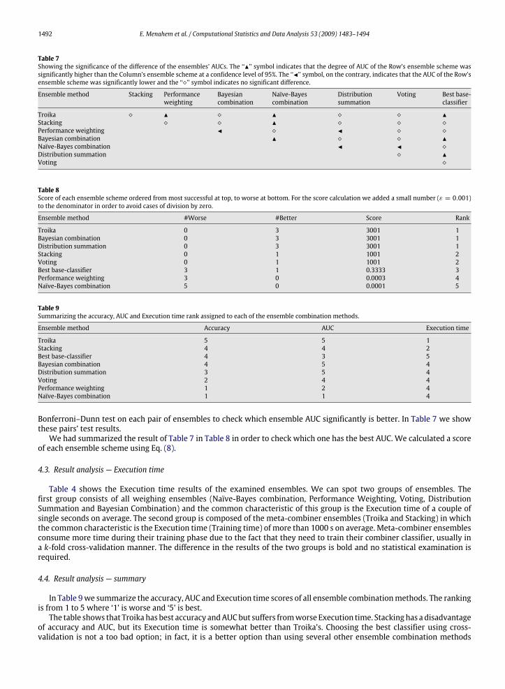
1492 E. Menahem et al. / Computational Statistics and Data Analysis 53 (2009) 1483–1494
Table 7Showing the significance of the difference of the ensembles’ AUCs. The ‘‘N’’ symbol indicates that the degree of AUC of the Row’s ensemble scheme wassignificantly higher than the Column’s ensemble scheme at a confidence level of 95%. The ‘‘J’’ symbol, on the contrary, indicates that the AUC of the Row’sensemble scheme was significantly lower and the ‘‘�’’ symbol indicates no significant difference.
Ensemble method Stacking Performanceweighting
Bayesiancombination
Naïve-Bayescombination
Distributionsummation
Voting Best base-classifier
Troika � N � N � � NStacking � � N � � �
Performance weighting J � J � �
Bayesian combination N � � NNaïve-Bayes combination J J �
Distribution summation � NVoting �
Table 8Score of each ensemble scheme ordered from most successful at top, to worse at bottom. For the score calculation we added a small number (ε = 0.001)to the denominator in order to avoid cases of division by zero.
Ensemble method #Worse #Better Score Rank
Troika 0 3 3001 1Bayesian combination 0 3 3001 1Distribution summation 0 3 3001 1Stacking 0 1 1001 2Voting 0 1 1001 2Best base-classifier 3 1 0.3333 3Performance weighting 3 0 0.0003 4Naïve-Bayes combination 5 0 0.0001 5
Table 9Summarizing the accuracy, AUC and Execution time rank assigned to each of the ensemble combination methods.
Ensemble method Accuracy AUC Execution time
Troika 5 5 1Stacking 4 4 2Best base-classifier 4 3 5Bayesian combination 4 5 4Distribution summation 3 5 4Voting 2 4 4Performance weighting 1 2 4Naïve-Bayes combination 1 1 4
Bonferroni–Dunn test on each pair of ensembles to check which ensemble AUC significantly is better. In Table 7 we showthese pairs’ test results.We had summarized the result of Table 7 in Table 8 in order to check which one has the best AUC. We calculated a score
of each ensemble scheme using Eq. (8).
4.3. Result analysis — Execution time
Table 4 shows the Execution time results of the examined ensembles. We can spot two groups of ensembles. Thefirst group consists of all weighing ensembles (Naïve-Bayes combination, Performance Weighting, Voting, DistributionSummation and Bayesian Combination) and the common characteristic of this group is the Execution time of a couple ofsingle seconds on average. The second group is composed of the meta-combiner ensembles (Troika and Stacking) in whichthe common characteristic is the Execution time (Training time) of more than 1000 s on average. Meta-combiner ensemblesconsume more time during their training phase due to the fact that they need to train their combiner classifier, usually ina k-fold cross-validation manner. The difference in the results of the two groups is bold and no statistical examination isrequired.
4.4. Result analysis — summary
In Table 9we summarize the accuracy, AUC and Execution time scores of all ensemble combinationmethods. The rankingis from 1 to 5 where ‘1’ is worse and ‘5’ is best.The table shows that Troika has best accuracy andAUCbut suffers fromworse Execution time. Stackinghas a disadvantage
of accuracy and AUC, but its Execution time is somewhat better than Troika’s. Choosing the best classifier using cross-validation is not a too bad option; in fact, it is a better option than using several other ensemble combination methods
E. Menahem et al. / Computational Statistics and Data Analysis 53 (2009) 1483–1494 1493
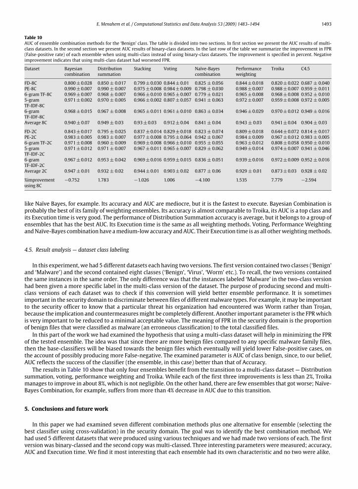
Table 10AUC of ensemble combination methods for the ‘Benign’ class. The table is divided into two sections. In first section we present the AUC results of multi-class datasets. In the second section we present AUC results of binary-class datasets. In the last row of the table we summarize the improvement in FPR(False-positive rate) of each ensemble when using multi-class instead of using binary-class datasets. The improvement is specified in percent. Negativeimprovement indicates that using multi-class dataset had worsened FPR.
Dataset Bayesiancombination
Distributionsummation
Stacking Voting Naïve-Bayescombination
Performanceweighting
Troika C4.5
FD-8C 0.800±0.028 0.850± 0.017 0.799±0.030 0.844±0.01 0.825± 0.056 0.844±0.018 0.820±0.022 0.687± 0.040PE-8C 0.990±0.007 0.990± 0.007 0.975±0.008 0.984±0.009 0.798± 0.030 0.988±0.007 0.988±0.007 0.959± 0.0116-gram TF-8C 0.969±0.007 0.968± 0.007 0.966±0.010 0.965±0.007 0.779± 0.021 0.965±0.008 0.968±0.008 0.952± 0.0105-gramTF-IDF-8C
0.971±0.002 0.970± 0.005 0.966±0.002 0.807±0.057 0.941± 0.063 0.972±0.007 0.959±0.008 0.972± 0.005
6-gramTF-IDF-8C
0.968±0.015 0.967± 0.008 0.965±0.011 0.961±0.010 0.863± 0.034 0.946±0.029 0.970±0.012 0.949± 0.016
Average 8C 0.940± 0.07 0.949± 0.03 0.93±0.03 0.912±0.04 0.841± 0.04 0.943± 0.03 0.941±0.04 0.904± 0.03
FD-2C 0.843±0.017 0.795± 0.025 0.837±0.014 0.829±0.018 0.823± 0.074 0.809±0.018 0.644±0.072 0.814± 0.017PE-2C 0.983±0.005 0.983± 0.007 0.977±0.008 0.795±0.064 0.942± 0.067 0.984±0.009 0.967±0.012 0.983± 0.0056-gram TF-2C 0.971±0.008 0.960± 0.009 0.969±0.008 0.966±0.010 0.955± 0.055 0.963±0.012 0.808±0.058 0.950± 0.0105-gramTF-IDF-2C
0.971±0.012 0.971± 0.007 0.967±0.011 0.965±0.007 0.829± 0.062 0.949±0.014 0.974±0.007 0.941± 0.046
6-gramTF-IDF-2C
0.967±0.012 0.953± 0.042 0.969±0.016 0.959±0.015 0.836± 0.051 0.939±0.016 0.972±0.009 0.952± 0.016
Average 2C 0.947± 0.01 0.932± 0.02 0.944±0.01 0.903±0.02 0.877± 0.06 0.929± 0.01 0.873±0.03 0.928± 0.02
%improvementusing 8C
−0.752 1.783 −1.026 1.006 −4.100 1.535 7.779 −2.594
like Naïve Bayes, for example. Its accuracy and AUC are mediocre, but it is the fastest to execute. Bayesian Combination isprobably the best of its family of weighting ensembles. Its accuracy is almost comparable to Troika, its AUC is a top class andits Execution time is very good. The performance of Distribution Summation accuracy is average, but it belongs to a group ofensembles that has the best AUC. Its Execution time is the same as all weighting methods. Voting, Performance WeightingandNaïve-Bayes combination have amedium-lowaccuracy andAUC. Their Execution time is as all otherweightingmethods.
4.5. Result analysis — dataset class labeling
In this experiment, we had 5 different datasets each having two versions. The first version contained two classes (‘Benign’and ‘Malware’) and the second contained eight classes (‘Benign’, ‘Virus’, ‘Worm’ etc.). To recall, the two versions containedthe same instances in the same order. The only difference was that the instances labeled ‘Malware’ in the two-class versionhad been given a more specific label in the multi-class version of the dataset. The purpose of producing second and multi-class versions of each dataset was to check if this conversion will yield better ensemble performance. It is sometimesimportant in the security domain to discriminate between files of differentmalware types. For example, it may be importantto the security officer to know that a particular threat his organization had encountered was Worm rather than Trojan,because the implication and countermeasuresmight be completely different. Another important parameter is the FPRwhichis very important to be reduced to a minimal acceptable value. The meaning of FPR in the security domain is the proportionof benign files that were classified as malware (an erroneous classification) to the total classified files.In this part of the work we had examined the hypothesis that using a multi-class dataset will help in minimizing the FPR
of the tested ensemble. The idea was that since there are more benign files compared to any specific malware family files,then the base-classifiers will be biased towards the benign files which eventually will yield lower False-positive cases, onthe account of possibly producing more False-negative. The examined parameter is AUC of class benign, since, to our belief,AUC reflects the success of the classifier (the ensemble, in this case) better than that of Accuracy.The results in Table 10 show that only four ensembles benefit from the transition to a multi-class dataset — Distribution
summation, voting, performance weighting and Troika. While each of the first three improvements is less than 2%, Troikamanages to improve in about 8%, which is not negligible. On the other hand, there are few ensembles that got worse; Naïve-Bayes Combination, for example, suffers from more than 4% decrease in AUC due to this transition.
5. Conclusions and future work
In this paper we had examined seven different combination methods plus one alternative for ensemble (selecting thebest classifier using cross-validation) in the security domain. The goal was to identify the best combination method. Wehad used 5 different datasets that were produced using various techniques and we had made two versions of each. The firstversion was binary-classed and the second copy was multi-classed. Three interesting parameters were measured; accuracy,AUC and Execution time. We find it most interesting that each ensemble had its own characteristic and no two were alike.
1494 E. Menahem et al. / Computational Statistics and Data Analysis 53 (2009) 1483–1494
From the results we learn that in terms of accuracy, and AUC, Troika is probably the best choice; it is better than Stacking,the only other ensemble in the group ofmeta-classifier ensembles. It is also better than the best classifier chosen using cross-validation. The benefit of using Troika is double; first, its AUC and accuracy are very high. Second, when using a multi-classdataset, its AUC improves in about 8%, producing a model with lower FPR and a nice capability of identifying the malware’sspecific class. Bayesian combination, for instance, being the second best in accuracy and AUC, had had a fall of 1% in its AUCperformance when tested on amulti-class dataset. If Execution time is a big concern, then Bayesian Combination will be thebest choice, being second only to Troika in terms of accuracy and AUC.We do not recommend using the Naïve-Bayes ensemble method.We can also see that the Naïve-Bayes ensemble method’s only good property is its fast Execution time which is the same
as all weighting methods. Its accuracy and AUC are fairly bad compared to all other ensembles. One explanation for its poorperformance is the fact that its assumptions are probably not taking place; for example, the assumption of independentbase-classifier does not exist in practice.Future work may include the involvement of more inducers for base-classifiers (we had only used 5, while there are
plentymore to choose from), some different methods of training the base-classifiers — in this researchwe had used only thetrivial trainingmethodwhile there aremany othermethods that use binarization of datasets (for example—One against Oneor One against All) which may yield better accuracy and AUC performance. In addition, in the hereby described experiment,we evaluated different inducers on the same datasets. In future experiments we would like to evaluate the performance ofinducers that are trained on different features.
Acknowledgment
This research is supported by Deutsche Telecom AG.
References
Abou-Assaleh, T., Cercone, N., Keselj, V., Sweidan, R., 2004. N-gram based detection of new malicious code. In: Proc. of the Annual International ComputerSoftware and Applications Conference, COMPSAC’04.
Buntine, W., 1990. A theory of learning classification rules. Doctoral Dissertation. School of Computing Science, University of Technology, Sydney.Caia, D.M., Gokhaleb,M., Theilerc, J., 2007. Comparison of feature selection and classification algorithms in identifyingmalicious executables. ComputationalStatistics and Data Analysis 51, 3156–3172.
Clark, P., Boswell, R., 1991. Rule induction with CN2: Some recent improvements. In: Proc. of the European Working Session on Learning, pp. 151–163.Demsar, J., 2006. Statistical comparisons of classifiers over multiple data sets. Journal of Machine Learning Research 7, 1–30.Dikinson, J., 2005. The new anti-virus formula. http://www.solunet.com/wp/security/How-to-use-multrd-security.pdf.Dzeroski, S., Zenko, B., 2004. Is combining classifiers with stacking better than selecting the best one? Machine Learning 54 (3), 255–273.Golub, T., et al., 1999. Molecular classification of cancer: Class discovery and class prediction by gene expression monitoring. Science 286, 531–537.Guvenir, G.D., 1997. Classification by voting feature intervals. In: Proc. of the European Conference on Machine Learning, pp. 85–92.Heidari, M., 2004. Malicious codes in depth. http://www.securitydocs.com/pdf/2742.pdf.Holte, R., 1993. Very simple classification rules perform well on most commonly used datasets. Machine Learning 11, 63–91.John, G.H., Langley, P., 1995. Estimating continuous distributions in Bayesian classifiers. In: Proc. of the Conference on Uncertainty in Artificial Intelligence,San Mateo, pp. 338–345.
Kabiri, P., Ghorbani, A.A., 2005. Research on intrusion detection and response: A survey. International Journal of Network Security 1 (2), 84–102.Kelly, C., Spears, D., Karlsson, C., Polyakov, P., 2006. An ensemble of anomaly classifiers for identifying cyber attacks. In: Proc. of the International SIAMWorkshop on Feature Selection for Data Mining.
Kibler, D.A., 1991. Instance-based learning algorithms. Machine Learning 37–66.Kienzle, D.M., Elder, M.C., 2003. Internet WORMS: Past, present, and future: Recent worms: A survey and trends. In: ACM Workshop on Rapid Malcode(WORM03).
Kittler, J., Hatef, M., Duin, R., Matas, J., 1998. On combining classifiers. IEEE Transactions on Pattern Analysis and Machine Intelligence 20 (3), 226–239.Kolter, J., Maloof, M., 2006. Learning to detect and classify malicious executables in the wild. Journal of Machine Learning Research 7, 2721–2744.Kuncheva, L.I., 2005. Diversity in multiple classifier systems (editorial). Information Fusion 6 (1), 3–4.Mahoney, M.V., 2003. A machine learning approach to detecting attacks by identifying anomalies in network traffic. Ph.D. Dissertation, Florida Tech.Menahem, E., 2008. Troika - An improved stacking schema for classification tasks. M.Sc. Thesis in Information System Engineering dep., Ben-GurionUniversity of the Negev, Israel.
Mitchell, T., 1997. Machine Learning. McGraw-Hill.Moskovitch, R., Elovici, Y., Rokach, L., 2008. Detection of unknown computer worms based on behavioral classification of the host. Computational Statisticsand Data Analysis 52 (9), 4544–4566.
Mukkamalaa, S., Sunga, A.H., Abrahamb, A., 2005. Intrusion detection using an ensemble of intelligent paradigms. Journal of Network and ComputerApplications 28, 167–182.
Opitz, D., Shavlik, J., 1996. Generating accurate and diverse members of a neural network ensemble. Advances in Neural Information Processing Systems8, 535–541.
Quinlan, R., 1993. C4.5: Programs for Machine Learning. Morgan Kaufmann Publishers.Schultz,M., Eskin, E., Zadok, E., Stolfo, S., 2001. Dataminingmethods for detection of newmalicious executables. In: Proc. of the IEEE Symposiumon Securityand Privacy, pp. 178–184.
Seewald, A.K., 2003. Towards understanding stacking — Studies of a general ensemble learning scheme. Ph.D. Thesis, TU Wien.Tumer, K., Ghosh, J., 1996. Error correlation and error reduction in ensemble classifiers. Connection Science 8, 385–404.Wang, K., Stolfo, S.J., 2004. Anomalous payload-based network intrusion detection. In: Proc. of International Symposium on Recent Advances in IntrusionDetection, RAID, pp. 1–12.
White, S., 1998. Open problems in computer virus research. IBM Research Center.White, S., 1999. Anatomy of a commercial-grade immune system. IBM Research Center.Witten, I.H., Frank, E., 2005. Data Mining: Practical Machine Learning Tools and Techniques, 2nd edition. Morgan Kaufmann, San Francisco. Retrieved on2007-06-25.
Wolpert, D.H., 1992. Stacked generalization. Neural Networks 5, 241–259.Zhang, B., Yin, J., Hao, J., Zhang, D., Wang, S., 2007. Malicious codes detection based on ensemble learning. Autonomic and Trusted Computing, 277–468.