18 : Theory of Production - NPTEL

1

18 : Theory of Production

Prof. Trupti Mishra, School of Management, IIT Bombay

Recap from last session Defining Input, Output, Production Production function Short Run Production Function Law of Diminishing Return


Session Outline Long Run Production Analysis Return to Scale Isoquants, Isocost Choice of input combination Expansion path Economic Region of Production

Returns to Scale

• The law of production describes the technically possible ways of increasing the level of output by changing all factors of production, which is possible only in the long run.

• Law of return to scale refers to long run analysis of production.


Returns to Scale

• It refers to the effects of scale relationship which implies that is long run output can be increased by changing all factors by the same or different proportion.


• If all inputs are increased by a factor of p & output goes up by a factor of z then, in general, a producer experiences:

Q = F (L,K)

ZQ = f(pL, pK)

Returns to Scale


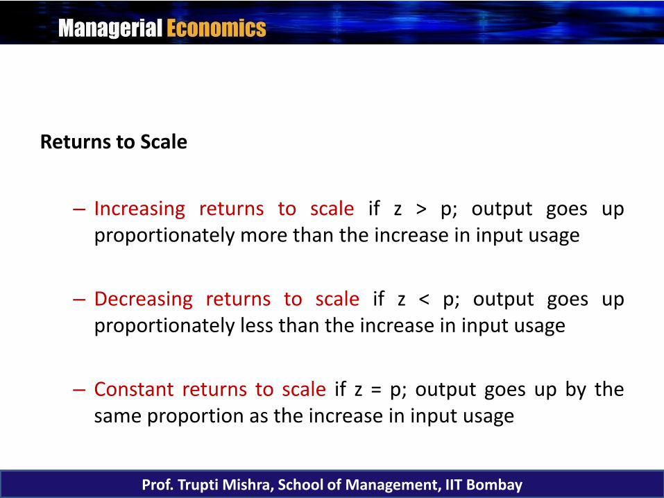
– Increasing returns to scale if z > p; output goes up proportionately more than the increase in input usage

– Decreasing returns to scale if z < p; output goes up proportionately less than the increase in input usage

– Constant returns to scale if z = p; output goes up by the same proportion as the increase in input usage

Returns to Scale


Returns to Scale and Homogeneity of the Production Function

If p can be factored out , then the new level of output can be expressed as ZQ = p v f(L, K) or ZQ = p v Q

This is called as homogeneous production function.

Q = F (L,K)

ZQ = f(pL, pK)


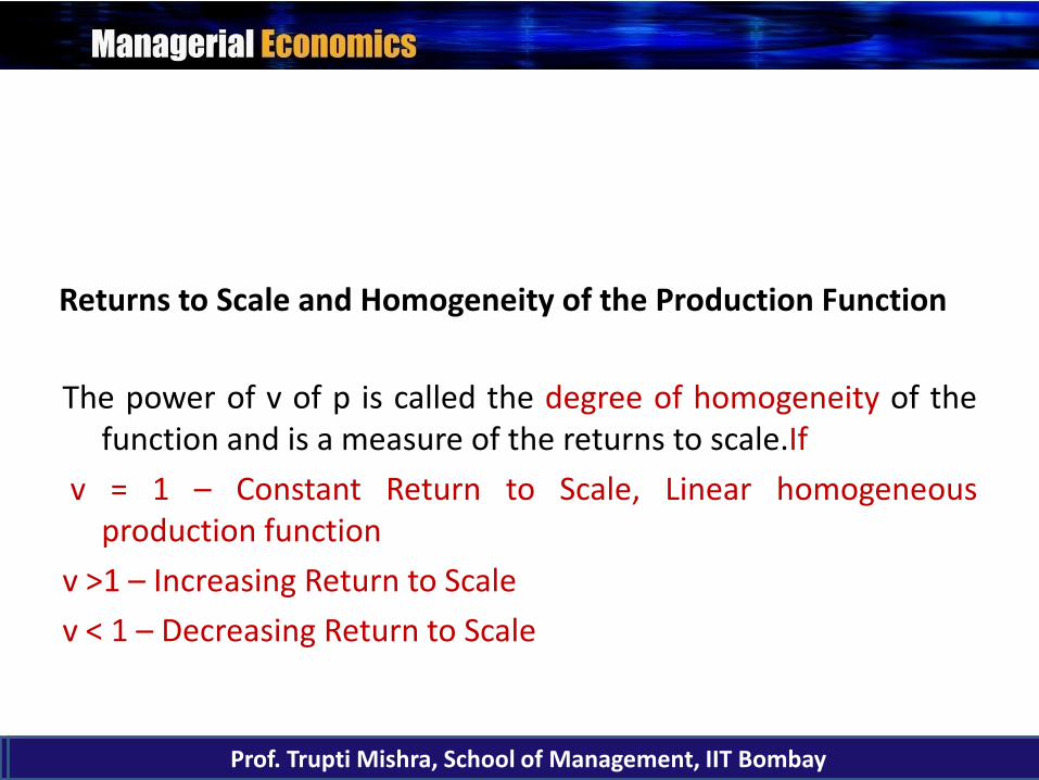
Returns to Scale and Homogeneity of the Production Function

The power of v of p is called the degree of homogeneity of the function and is a measure of the returns to scale.If

v = 1 – Constant Return to Scale, Linear homogeneous production function

v >1 – Increasing Return to Scale

v < 1 – Decreasing Return to Scale


Returns to Scale -Example

• Q = K0.25L0.50

If K and L are multiplied by k, and output increases by a multiple of h, then hQ = (kK)0.25(kL)0.50.

factoring out k, hQ = k0.25 + 0.50[K0.25L0.50]

• = k0.75[K0.25L0.50]

h = k0.75 and r = 0.75, implying that r < 1, and, h < k. It follows that the production function shows decreasing returns to scale.


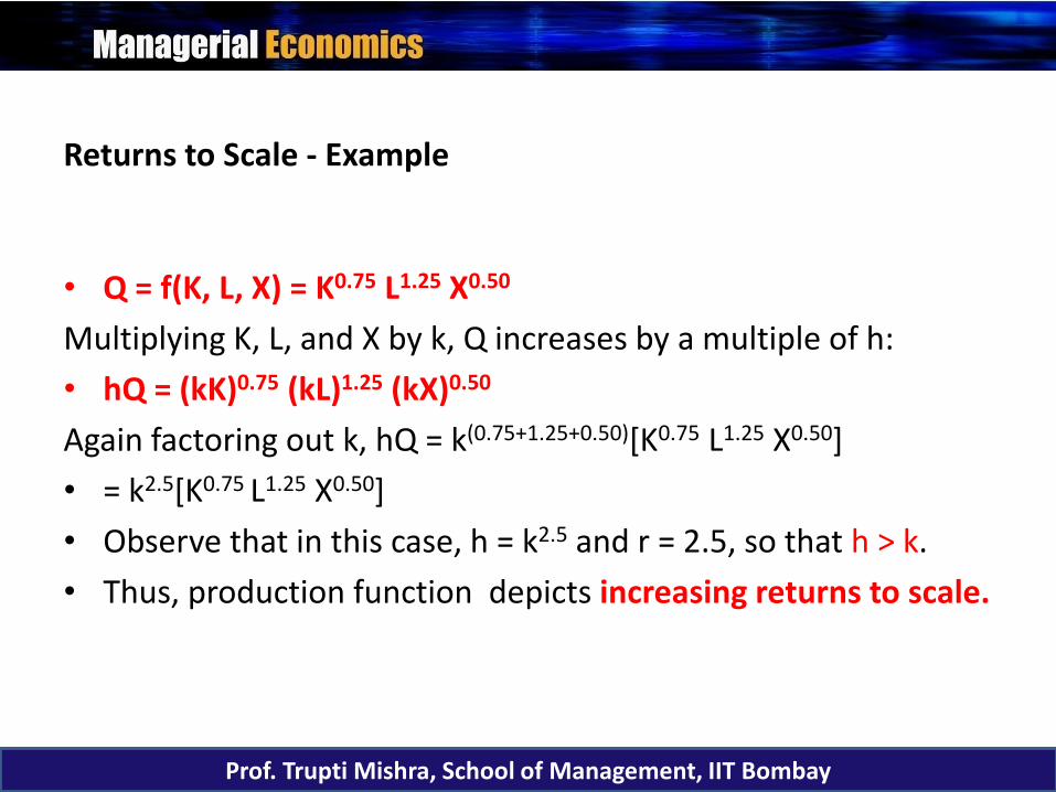
Returns to Scale - Example

• Q = f(K, L, X) = K0.75 L1.25 X0.50

Multiplying K, L, and X by k, Q increases by a multiple of h:

• hQ = (kK)0.75 (kL)1.25 (kX)0.50

Again factoring out k, hQ = k(0.75+1.25+0.50)[K0.75 L1.25 X0.50]

• = k2.5[K0.75 L1.25 X0.50]

• Observe that in this case, h = k2.5 and r = 2.5, so that h > k.

• Thus, production function depicts increasing returns to scale.


• In the long run, all inputs are variable & Isoquant are used to study production decisions

- An Isoquant is the firm’s counterpart of the consumer’s indifference curve.

Isoquant


– An Isoquant is a curve showing all possible input combinations capable of producing a given level of output

– Isoquant are downward sloping; if greater amounts of labor are used, less capital is required to produce a given output

Isoquant


Typical Isoquants


• The MRTS is the slope of an Isoquant & measures the rate at which the two inputs can be substituted for one another while maintaining a constant level of output

KMRTS

L

Marginal Rate of Technical Substitution


• If the law of diminishing marginal product operates, the Isoquant will be convex to the origin.

• A convex Isoquant means that the MRTS between L and k decreases as L is substituted for K.



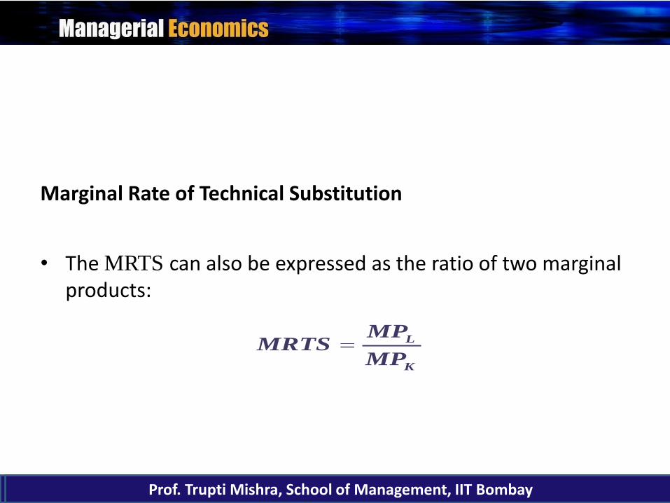
• The MRTS can also be expressed as the ratio of two marginal products:

L

K

MPMRTS

MP



L

K

MP

MP MRTS

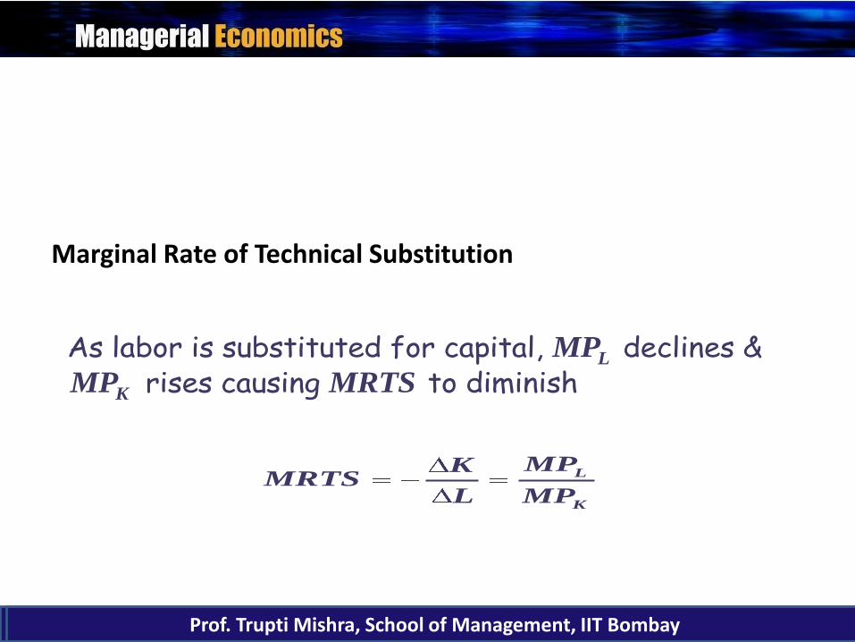
As labor is substituted for capital, declines &rises causing to diminish

L

K

MPKMRTS

L MP



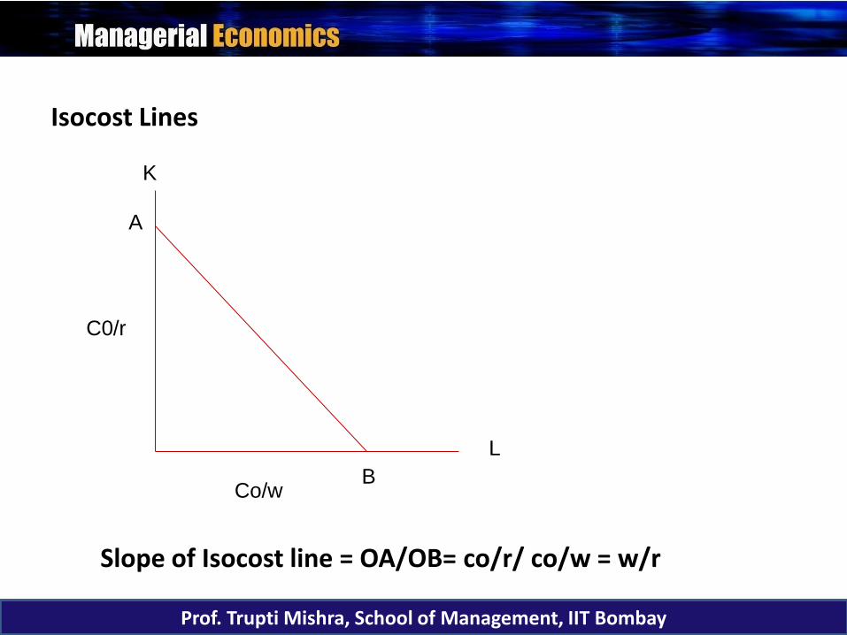
Isocost Lines

• Shows various combination of inputs which may be purchased for given level of cost and price of inputs.

• Co = w.L + r.K

• This equation will be satisfied by different combinations of L and K. the locus of all such combinations is called equal cost line/ or isocost line.


Isocost Lines

Co/w

C0/r

A

B

K

L

Slope of Isocost line = OA/OB= co/r/ co/w = w/r


Q

Q

Minimize total cost of producing by

choosing the input combination on the

isoquant for which is just tangent to an

isocost curve

•

Optimal Combination of Inputs


– Two slopes are equal in equilibrium

– Implies marginal product per dollar spent on last unit of each input is the same

L L K

K

MP MP MPw

MP r w ror

Optimal Combination of Inputs


• The expansion path is locus of all input combinations for which the MRTS is equal to the factor price ratio.

• The locus of all such points of tangencies between the Isoquant and the parallel Isocost lines is the expansion path for the firm.

Expansion path


• Expansion path gives the efficient (least-cost) input combinations for every level of output

• Along expansion path, input-price ratio is constant & equal to the marginal rate of technical substitution

Expansion path


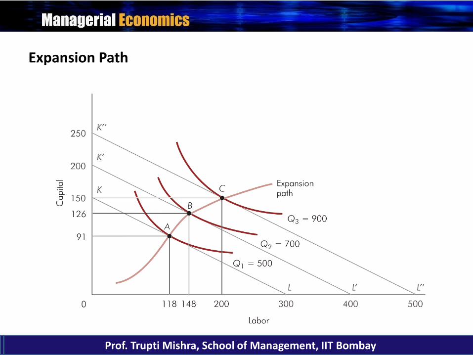
Expansion Path


Expansion path

• If both the factors of production are non-inferior, the expansion path will be upward rising. In this case more of both the factors will be required for producing more of output.


Expansion path

• If the production function is homogeneous the expansion path will be a straight line through the origin whose slope depends on the ratio of factor prices.

• If the production function is non-homogeneous then the optimal expansion path will not be a straight line , even if the ratio of factor prices remain constant.


Economic Region of Production

• There exist a range over which one input can be substituted for the other, within that range isoquants are negatively sloped.

• Efficient range of output: the range over which the marginal products of the factors are diminishing but positive.



• Production does not take place when MP of the factor is negative.

• The locus of points of isoquants where the marginal products are zero form the Ridge line.



• Production techniques are technically efficient inside the ridge line. Outside the ridge lines the marginal products of the factors are negative and the method of production are inefficient as they require more quantity of both the factors for producing a given level of output.

• The range of isoquants over which they are convex to origin defines the range of efficient production.



• The upper ridge line implies that MP of capital is zero and lower ridge line implies MP of labor is zero.

• In isoquant Q0, A1 and A2 be the point where tangents are drawn are parallel to the vertical and horizontal axes respectively.



• That portion of the isoquant which lies between A1 and A2 , is the portion within which substitution takes place.

• Between A1 and A3, at A3 more of both factors required to produce the same level of output .



• Along the isoquant Qo, proceeding downwards, the marginal product of labor will decrease and MP of capital will increase, and vice versa.

• At the point of A1 and A2, the slope of isoquant Qo is infinity and Zero respectively.



• Slope = - MPL/MPK. This means that at point A1, MPK= 0, and at point A2 , MPL = 0.

• So the portion A1A2 lies within the ridge lines and called the economic region of production.


• It is only within A1 and A2 that both MPL and MPK are positive and the isoquant is downward sloping.

• The equation of upper ridge line is given by MPK = 0, and the equation of the lower ridge line is given by MPL =0



Session References

36

Managerial Economics; D N Dwivedi, 7th Edition Managerial Economics – Christopher R Thomas, S Charles Maurice and Sumit Sarkar Micro Economics : ICFAI University Press


18 : Theory of Production - NPTEL

Documents

Transcript of 18 : Theory of Production - NPTEL