1 23

Theoretical and Applied Climatology ISSN 0177-798X Theor Appl ClimatolDOI 10.1007/s00704-013-0947-4

Differences between two climatologicalperiods (2001–2010 vs. 1971–2000)and trend analysis of temperature andprecipitation in Central Brazil

Pablo de Amorim Borges, JohannesFranke, Fabrício Daniel do Santos Silva,Holger Weiss & Christian Bernhofer

1 23

Your article is protected by copyright and

all rights are held exclusively by Springer-

Verlag Wien. This e-offprint is for personal

use only and shall not be self-archived

in electronic repositories. If you wish to

self-archive your article, please use the

accepted manuscript version for posting on

your own website. You may further deposit

the accepted manuscript version in any

repository, provided it is only made publicly

available 12 months after official publication

or later and provided acknowledgement is

given to the original source of publication

and a link is inserted to the published article

on Springer's website. The link must be

accompanied by the following text: "The final

publication is available at link.springer.com”.

ORIGINAL PAPER

Differences between two climatological periods (2001–2010vs. 1971–2000) and trend analysis of temperatureand precipitation in Central Brazil

Pablo de Amorim Borges & Johannes Franke &

Fabrício Daniel do Santos Silva & Holger Weiss &

Christian Bernhofer

Received: 22 November 2012 /Accepted: 3 June 2013# Springer-Verlag Wien 2013

Abstract In the framework of the IWAS/Água-DF project,this study focuses on changes in mean surface air tempera-ture and accumulated precipitation in Central Brazil over thepast 40 years. It has two main objectives: (1) comparisonbetween two climatological periods (2001–2010 and 1971–2000) and (2) trend analysis of climate variables. Time seriesof meteorological and rain gauge stations from CentralBrazil have been organized in a databank, which containstools for homogeneity tests. From that, 4 temperature and 55precipitation time series were sufficient homogeneous, while1 temperature and 5 precipitation time series were identifiedas inhomogeneous. Reliable spatial distribution was pro-duced using proper interpolation method. Trends and signif-icance levels were calculated by Rapp’s estimator of slopeand Mann–Kendall test, respectively. The most importantresults of the comparisons and trend analysis in the last fourdecades are: (1) marked increase in annual and seasonalmean surface air temperature, (2) evident decreases of accu-mulated rainfall in winter and autumn, and (3) apparentincrease of precipitation amounts in the rainy season.

1 Introduction

As a consequence of accelerated nonplanned urbanization,changes in land use, and predicted impacts of climatechange, the capital city of Brazil is suffering an increasingstress on its water resources. Predictions of the local watersupplier (i.e., Environmental Sanitation Company of theFederal District—CAESB) state that water demand will ex-ceed the systems supply capability already at the beginning ofthe second decade of the twenty-first century. Facing theurgency to take action that will guarantee the water supplyof Brasilia, the project called IWAS/Água-DF (InternationalWater Research Alliance Saxony) aims to develop an integrat-ed water resources management system, which considers nat-ural boundary conditions (i.e., climate, hydrological cycle,and land use), water supply systems (i.e., drinking and sewagewater treatment and distribution system), and managementissues. In order to achieve this goal, the project is organizedin a toolbox concept with climate data as an essential input(Lorz et al. 2012). Up to now, global circulation models(GCMs) are the most preferential tools to simulate the re-sponse of a climate system to increasing global anthropogenicactivities, for instance land use and greenhouse gas concen-trations (Lu 2006; Dobler et al. 2012). However, the climateinformation required for water resources management is of aspatial scale much finer than that provided by global models,and, therefore, regional climate models are often required(Bárdossy and Pegram 2011; Wilby and Dawson 2012).Although many regionalization techniques such as dynamicand statistical downscaling are available, all of them rely in theprinciple that GCM output is used as initial and lateral bound-ary conditions (Pavlik et al. 2012). Nevertheless, downscalingmethods demand a recent and spatially detailed climate

P. A. Borges (*) : J. Franke :C. BernhoferInstitute of Hydrology and Meteorology, Technische UniversitätDresden (TU Dresden), 01737, Tharandt, Germanye-mail: pablo.borges@ufz.de

F. D. do Santos SilvaCoordenação Geral de Desenvolvimento e Pesquisa—CDP,Instituto Nacional de Meteorologia—INMET, 70680-900, Brasília,Federal District, Brazil

H. WeissDepartment Groundwater Remediation, Helmholtz Center forEnvironmental, Research GmbH—UFZ, 04318, Leipzig, Germany

Theor Appl ClimatolDOI 10.1007/s00704-013-0947-4

Author's personal copy

diagnosis of the region, either for calibration and validationpurposes or as a benchmark for comparisons (IPCC-TGCIA1999).Moreover, the study region is under the influence of theSouth American monsoon system (SAMS) (Zhou and Lau1998; Vera et al. 2006). A systematic analysis of observedclimatic variability can contribute to a better understanding ofthe components of the SAMS and its influence over CentralBrazil during the period considered in this study. Likewise,available historical and current climate studies in CentralBrazil do not provide the necessary spatial and temporalresolution for detailed climate diagnosis, as they do not satisfythe requirements for developing regional climate scenarios.

In this framework, this study focuses on changes in meansurface air temperature and accumulated precipitation inCentral Brazil in the last four decades. It has three specificobjectives: (1) perform quality and homogeneity tests of allavailable daily data in the study region, (2) develop spatialdistribution maps of mean surface air temperature and rainfall,(3) investigate regional climate variability through compari-sons between two periods (2001–2010 and 1971–2000), and(4) perform long-term trend analysis and test the significance.

2 Database

The databank comprises daily values of two climate variables:mean surface air temperature (in degrees Celsius) and accumu-lated precipitation (in millimeter). Additional data in the data-base, but not used in the study, include relative humidity, solar

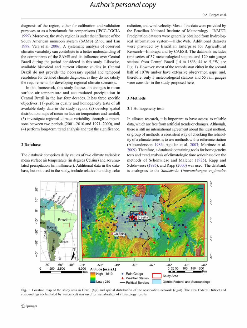
radiation, and wind velocity. Most of the data were provided bythe Brazilian National Institute of Meteorology—INMET.Precipitation datasets were generally obtained from hydrolog-ical information system—HidroWeb. Additional datasetswere provided by Brazilian Enterprise for AgriculturalResearch—Embrapa and by CAESB. The databank includestime series of 37 meteorological stations and 120 rain gaugestations from Central Brazil (14 to 18°S; 44 to 51°W, seeFig. 1). However, most of the records start either in the secondhalf of 1970s and/or have extensive observation gaps, and,therefore, only 5 meteorological stations and 55 rain gaugeswere consider in the study proposed here.

3 Methods

3.1 Homogeneity tests

In climate research, it is important to have access to reliabledata, which are free from artificial trends or changes. Although,there is still no international agreement about the ideal method,or group of methods, a consistent way of checking the reliabil-ity of a climate series is to use methods with a reference station(Alexandersson 1986; Aguilar et al. 2003; Martínez et al.2009). Therefore, a databank containing tools for homogeneitytests and trend analysis of climatologic time series based on themethods of Schönwiese and Malcher (1985), Rapp andSchönwiese (1995), and Rapp (2000) was used. The databankis analogous to the Statistische Untersuchungen regionaler

Fig. 1 Location map of the study area in Brazil (left) and spatial distribution of the observation network (right). The area Federal District andsurroundings (delimitated by watershed) was used for visualization of climatology results

P.A. Borges et al.

Author's personal copy

Klimatrends in Sachsen—CLISAX databank, which is a rela-tional database system consisting of three sub-databanks,where all procedures (i.e., data assimilation, data analysis,and data readout) are performed by modules, as described byFranke et al. (2004) and applied in Bernhofer et al. (2008a) andBernhofer et al. (2008b). At the first step, the tool assimilatesdata of climate values, import related information of eachstation, and calculates several statistical parameters of the timeseries. The tool is able to check for suspicious values, errors,and outliers by a one- or two-tailed test after Dixon (1950).Next, the homogeneity of the data is represented by graphical(i.e., Craddock test, double sum analysis, quotient criteria, anddifference in limits) and numerical tests (i.e., Abbe, Buishand,and standard normal homogeneity test—SNHT) (Craddock1956; Buishand 1982; Alexandersson 1986; Dahmen andHall 1990; Herzog and Müller-Westermeier 1998). The ap-proach has a limit concerning to gaps, and therefore, a timeseries is neglected if missing values excess 25 % of the data ina regarding month. Considering the spatial distribution of theclimate stations, the homogeneity tests were performed startingfrom a known homogeneous station, for instance the mainstation of INMET in Brasília, in which metadata are well-documented. This station was used as reference for near-neighbor stations. Once the homogeneity was tested, thenear-neighbor stations were used as a reference for furtherneighbor stations, and so on until all stations in the domainarea were tested. In case of inhomogeneity of a time series,metadata is checked, homogenization procedure is performed,and complete test cycle is repeated until homogeneity isreached.

3.2 Climatological normals

Climatological normals are basic information to classify aregion’s climate and are recommended as a description of theaverage climatic conditions of a certain region (Trewin2007). Therefore, climatological periods (i.e., 30-year nor-mals, as 1971–2000 and decades, as 2001–2010) were cal-culated according to the suggestions of WMO (1989), whichestablishes general procedures to be used for the calculationof monthly and annual 30-year standard and provisionalnormals for climate data. Before calculating monthly andannual climatologies and trend analysis, an estimation ofmissing monthly mean temperature and total precipitation,using difference and ratio criterion respectively, wasperformed according to Bernhofer (2004). Following the“3/5 rule” for missing data in climatology calculation(WMO 1989; Trewin 2007), some stations starting after1971 may also be useful for the 1971–2000 climatology. Inorder to increase the number of stations used, the monthlyfill-gaps method was also applied for observations startinguntil 1974 that agree with the “3/5 rule”.

3.3 Spatial interpolation

Since observations are taken from single points, interpola-tion is an important task in the development of spatial distri-bution representations. A large variety of interpolationmethods are available. Before selecting the proper one, it isnecessary to consider the purpose of the interpolation, thecharacteristics of the phenomena to be analyzed, and theconstraints and assumptions of the technique (Wackernagel2003; Dyras et al. 2005; Renard and Comby 2006). Manyapplications for establishing reliable spatial representationsof temperature and precipitation rely on the principle ofresidual interpolation, or detrended interpolation, where theinfluence of different terrain characteristics in addition to afew other external parameters are used to describe the globaltrend expression (Nalder and Wein 1998; Tveito and Førland1999; Lhotellier 2005). Borges et al. (2013) compared withseveral spatial interpolation methods for seasonal and annual30-year precipitation in Central Brazil. Between most com-monly used methods, such as universal Kriging and inversedistance weighting (IDW), the multivariate regression modelusing altitude, latitude, and longitude as explanatoryvariables, with interpolation of residuals by IDW (i.e.,MRegIDW), performed the most reliable and detailedpredictions according to visual analysis and statisticalcriteria such as mean square error, correlation coeffi-cient, and Nash–Sutcliffe criterion (Nash and Sutcliffe1970). In order to reduce the interpolation uncertaintiesin the boundaries of the study region, the data obtainedfrom Central Brazil region are illustrated only for thedomain area of Federal District and surroundings.

3.4 Trend analysis

Last but not least, the detection of trend is of a remark-able interest in climate impact studies. This is essentialinformation to drive decisions in water resource man-agement (Helsel and Hirsch 2002; Karpouzos et al.2010). As demonstrated by many authors (Rapp 2000;Franke et al. 2004; Bernhofer et al. 2008a, b), thisstudy investigates the variability of mean surface airtemperature, as well as precipitation, at seasonal andannual time scale. Linear trends in the temporal struc-ture of long-term time series were detected by applyingRapp (2000), for calculation of the slope, and Mann–Kendall (Mann 1945; Kendall 1970) method to assessthe significance of the trends. In order to identify lineartrends from the statistic variability of time series, theregression form was obtained:

y tð Þ ¼ aþ β ⋅ t ð1Þ

Differences between two climatological periods

Author's personal copy

Where the slope β was calculated by:

β ¼

12

N⋅XN

n¼1

tn⋅ynð Þ− N þ 1

2

XN

n¼1

yn

!

N 2−1ð2Þ

With n=1,…,N and the concerning value yn at the time tn.The absolute trend Tabs results from the difference of the firstand last ordinate of the regression line, and it is given as:

Tabs ¼ yn−y1 ¼ β ⋅ N−1ð Þ ð3ÞThe relative trend Trel is a normalization of Tabs with the

mean of the values yover the considered time interval and isindicated as (percent).

Trel ¼ Tabs

yð4Þ

Trend liability cannot be interpreted without informa-tion about the statistical trustworthiness. In statistics,security is interpreted as significance level, and, in thiscontext, means that the trend should explicitly lay be-yond the time series normal variability (Bernhofer et al.2008a). The Mann–Kendall test is a robust nonparamet-ric test for monotonic trends, which compares the rela-tive amount of sample data rather than the data valuesthemselves (Helsel and Hirsch 2002; Birsan et al. 2005).The major advantages are: (1) It can be applied in caseof data containing outliers, and (2) time series do notneed to conform to any particular distribution, such asnormally distributed data and linear trends (Salas 1993;Helsel and Hirsch 2002; Birsan et al. 2005). To test thesignificance of the trends, this study applied the signif-icance level (SIG) as follows:

Q ¼

XN−1

i¼1

XN

j¼iþ1

sgn y j − yi� �

ffiffiffiffiffiffiffiffiffiffiffiffiffiffiffiffiffiffiffiffiffiffiffiffiffiffiffiffiffiffiffiffiffiffiffiffiffiffiffiffiffiffiffiffiffiffiffiffiffiffiffiffiffiffiffiffiffiffiffiffiffiffiffiffiffiffiffiffiffiffiffiffiffiffiffiffiffiffiffiffiffiffiffiffiffiffiffiffiffiffiffiffiffiffiffiffiffiffiffiffiffiffiffiffiffiffiffiffiffiffiffiffiffiffiffiffiffiffiffiffiffiffiffiffiffiffiffiffiffiffi1

18N N − 1ð Þ ⋅ 2N þ 5ð Þ −

X

I

bI bI − 1ð Þ ⋅ 2bI þ 5ð Þ" #vuut

ð5Þ

Where N is the length of the analyzed time series, yi and yjare the observation values to be compared, sgn is the direc-tional information, and bI means the number of values of theobservation value yI. The summation in Eq. (5) over allpossible pairs (yi, yj) is possible when i< j. This form pro-vides the Mann–Kendall test numbers Q, where the signifi-cance can be specified as significance levels SIG (Table 1).

4 Results

4.1 Homogeneity tests

The homogeneity of the data used in this study was testedusing a complex algorithm set (Franke et al. 2004). Theapproach has a limit concerning to gaps, and therefore, a time

series is neglected if missing values excess 25 % of the data ina regarding month. Since the purpose here is to investigatedifferences and trends of the period from beginning of 70suntil 2010, observations starting later than 1974 were exclud-ed. In order to not distort the values for subsequent work, thehomogenization of time series was very conservative. In allcases of homogenization, non-homogeneities were very ex-plicit, especially by SNHT. Causes were confirmed in themetadata of the stations, either by station relocation or mea-surement device alteration. Table 2 shows an overview of thehomogeneity tests. From 37mean surface air temperature timeseries, 4 were considered satisfactorily homogeneous, while 1was inhomogeneous, and 32 could not be tested due to insuf-ficient data. Moreover, precipitation time series were consid-ered homogeneous in 55 cases, whereas 5 were recognized asinhomogeneous and 97 are over the gap limit or observationsstarted later than 1974.

4.2 Mean surface air temperature

4.2.1 Spatial variability

The spatial distribution of mean surface air temperature de-pends mainly on geographic position and topography, varyingfrom low regions, which register high temperatures, to elevat-ed region—such as the Goiás highlands—where milder

Table 1 Significance level SIG of trends

Q SIG Q SIG From Schönwiese (2000)

>1 >68.3 % >1.28 >80 %

>1.5 >86.6 % >1.65 >90 % Significant

>2 >95.4 % >1.96 >95 % Very significant

>3 >99.7 % >2.58 >99 % Highly significant

>4 >99.99 % >3.29 >99.9 % Extremely significant

P.A. Borges et al.

Author's personal copy

temperatures are observed (Alves 2009). Results show a gra-dient in annual mean temperature of about 0.7 °C/100m. OverFederal District and surroundings, the annual mean tempera-ture for the normal climatological period (i.e., 1971–2000) is22.2 °C. Nevertheless, rates vary between approximately 19.4and 24.5 °C (Fig. 2a). Generally, the warmest regions are thelowlands in northwest, northeast, and southeast. While thehighlands in Federal District and Goiás plateaus (i.e., north)have milder temperatures. The warmest season registered wasspring (SON), with average temperature of 23.2 °C, followedby summer (DJF) 22.6 °C, and autumn (MAM) 22.0 °C(Fig. 3d, a and b, respectively). This phenomenon is explaineddue to maximum solar radiation incidence over Central Brazilfrom the spring equinox (September) until the summer solstice(December) associated with the influence of a monsoon re-gime (Zhou and Lau 1998). Low-level jets (LLJ) bring in-creasing temperature and humidity from the Amazon toCentral Brazil starting in September. From that untilFebruary prevails trade winds from the North Tropical

Atlantic, which converges to Central Brazil due to AndesCordillera (Gan et al. 2004). Around April, LLJ flows overCentral Brazil changes the direction due to the decrease oftrade winds and intensification of the northwest flux associat-ed with the South Atlantic subtropical anticyclone (Marengoet al. 2009). In addition, due to less solar radiation and ingressof cold air masses from south, average temperature in winter(JJA) is milder 21.2 °C. At the same season, mean temperaturein high areas can reach 17.9 °C (Fig. 3c).

Comparisons between the climatological period 2001–2010and the normal 1971–2000 describe considerable increase inmean temperature. In average, the difference in annual meantemperature rely on +0.7 °C (Fig. 2b). The highest divergences(>+1.0 °C) were observed in southeast parts of the study area.Concerning the seasons, spring recorded the highest increasesin mean temperature of about +1.0 °C (Fig. 4d) in average. Thesecond most relevant variation was observed in summer, +0.7 °C (Fig. 4a). Differences in autumn and winter are 0.6 and0.4 °C (Fig. 4b and c), respectively. However, due to the lack of

Table 2 Status of the databank concerning to the homogeneity of the time series (number of stations) for the period from 1971 to 2010

Climate variable Status

Homogeneous Inhomogeneous Insufficient dataa Total

Mean surface air temperature 4 1 32 37

Precipitation 55 5 97 157

Bold number stations used; Italic number of stations neglecteda Insufficient data due either to excess of missing data or records starting after 1974

Fig. 2 a Annual mean surface air temperature over the Federal District and surroundings for the normal period 1971–2000 and b the differences ofthe period 2001–2010

Differences between two climatological periods

Author's personal copy

observations in the east and southeast, the uncertainty of thespatial interpolation method is the highest in this region, andtherefore results must be careful interpreted (Borges et al.2013).

4.2.2 Long-term trends

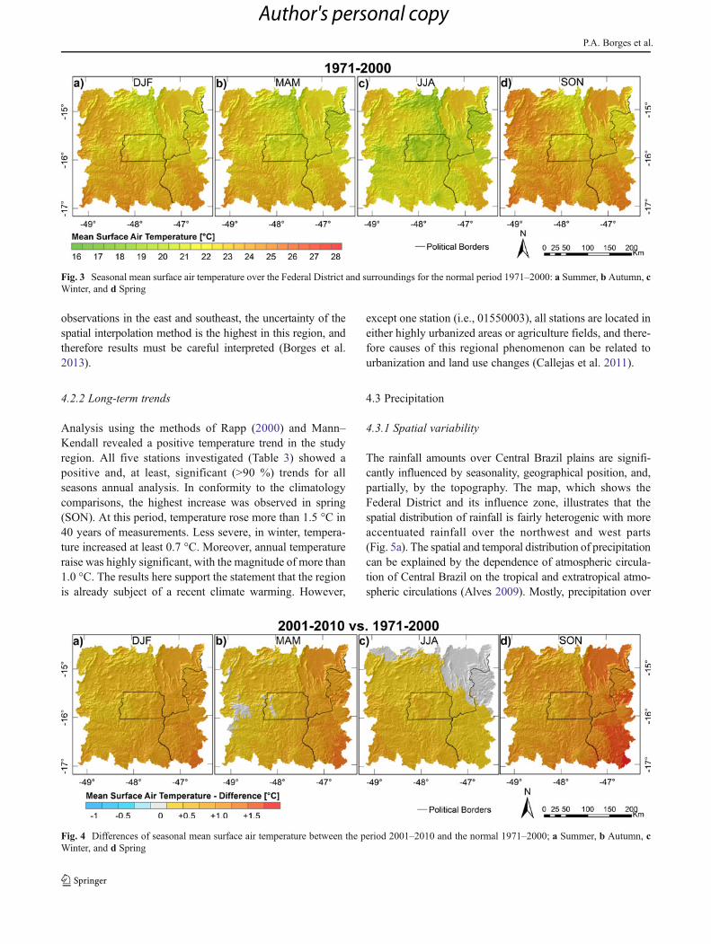
Analysis using the methods of Rapp (2000) and Mann–Kendall revealed a positive temperature trend in the studyregion. All five stations investigated (Table 3) showed apositive and, at least, significant (>90 %) trends for allseasons annual analysis. In conformity to the climatologycomparisons, the highest increase was observed in spring(SON). At this period, temperature rose more than 1.5 °C in40 years of measurements. Less severe, in winter, tempera-ture increased at least 0.7 °C. Moreover, annual temperatureraise was highly significant, with the magnitude of more than1.0 °C. The results here support the statement that the regionis already subject of a recent climate warming. However,

except one station (i.e., 01550003), all stations are located ineither highly urbanized areas or agriculture fields, and there-fore causes of this regional phenomenon can be related tourbanization and land use changes (Callejas et al. 2011).

4.3 Precipitation

4.3.1 Spatial variability

The rainfall amounts over Central Brazil plains are signifi-cantly influenced by seasonality, geographical position, and,partially, by the topography. The map, which shows theFederal District and its influence zone, illustrates that thespatial distribution of rainfall is fairly heterogenic with moreaccentuated rainfall over the northwest and west parts(Fig. 5a). The spatial and temporal distribution of precipitationcan be explained by the dependence of atmospheric circula-tion of Central Brazil on the tropical and extratropical atmo-spheric circulations (Alves 2009). Mostly, precipitation over

Fig. 3 Seasonal mean surface air temperature over the Federal District and surroundings for the normal period 1971–2000: a Summer, b Autumn, cWinter, and d Spring

Fig. 4 Differences of seasonal mean surface air temperature between the period 2001–2010 and the normal 1971–2000; a Summer, b Autumn, cWinter, and d Spring

P.A. Borges et al.

Author's personal copy

Central Brazil is a result of the convergent flow of humidity atthe low troposphere coming from the Amazon region (Kousky1988). In the Equatorial Atlantic region, low-level east windsare deviated from northwest toward southeast due to theAndes barrier, bringing intensive rainfall over Central Brazil,especially between December and February (Gan et al. 2004;Vera et al. 2006). Rainfall events can be intensified due to theSouth Atlantic convergence zone (SACZ), which is a band ofcloudiness and rainfall which extends over Amazon region tothe subtropical Atlantic ocean with orientation northeast–southwest (Carvalho and Jones 2009). This circulation canaffect the regional climate in many manners, including ex-treme events associated to mesoscale convective systems(MCS) (Maddox 1980). Topography also assists rainfallmechanisms by forcing the air lift in higher areas, as in westof the Federal District, creating greater convective activitycompared to areas downwind of these natural highs. It is

expected that the high areas in northwest and west are undermore influence of the moisture coming from the Amazon thansoutheast low part, where rainfall is less.

Considering the climatological normal period (i.e., 1971–2000), the average in accumulated annual precipitation overall the study area is about 1,418 mm. However, differencesdue to geographic position can reach more than 500 mm.Substantial differences were also observed in DistritoFederal. The western part shows annual precipitations ofaround 1,500 mm, while 50 km eastern, precipitations canbe less than 1,350 mm.

Similar spatial distribution is observed in summer and lessapparent in autumn and spring (Fig. 6a, b, and d) due to thefact that the SACZ occurs from mid-October until end ofMarch (Carvalho et al. 2004). From December to February,when the MCS are more common due to the LLJ insertion,accentuated precipitation associated with extreme events is

Table 3 Trend analysis of seasonal and annual mean surface air temperature

Station ID DJF MAM JJA SON Annual

Abs (°C) SIG (%) Abs (°C) SIG (%) Abs (°C) SIG (%) Abs (°C) SIG (%) Abs (°C) SIG (%)

01547004 +0.7 >99 +0.8 >99 +0.7 >95.4 +1.5 >99.7 +1.1 >99.7

01547016 +1.6 >99.9 +0.8 >95.4 +0.7 >95.4 +2.1 >99.99 +1.3 >99.99

01548014 +1.1 >99.9 +1.3 >99.9 +1.0 >99 +1.9 >99.99 +1.3 >99.99

01550003 +1.0 >99 +0.9 >95.4 +0.8 >90 +1.7 >99.9 +1.1 >99.9

01649013 +1.0 >99.7 +1.2 >99.7 +1.5 >99.7 +1.9 >99.99 +1.6 >99.7

SIG level >86.6 % = significant, >95.4 % = very significant, >99.7 % = highly significant and NS not significant (after Schönwiese 2000)

Fig. 5 a Annual accumulated precipitation over the Federal District and surroundings for the normal period 1971–2000 and b the differences of theperiod 2001–2010

Differences between two climatological periods

Author's personal copy

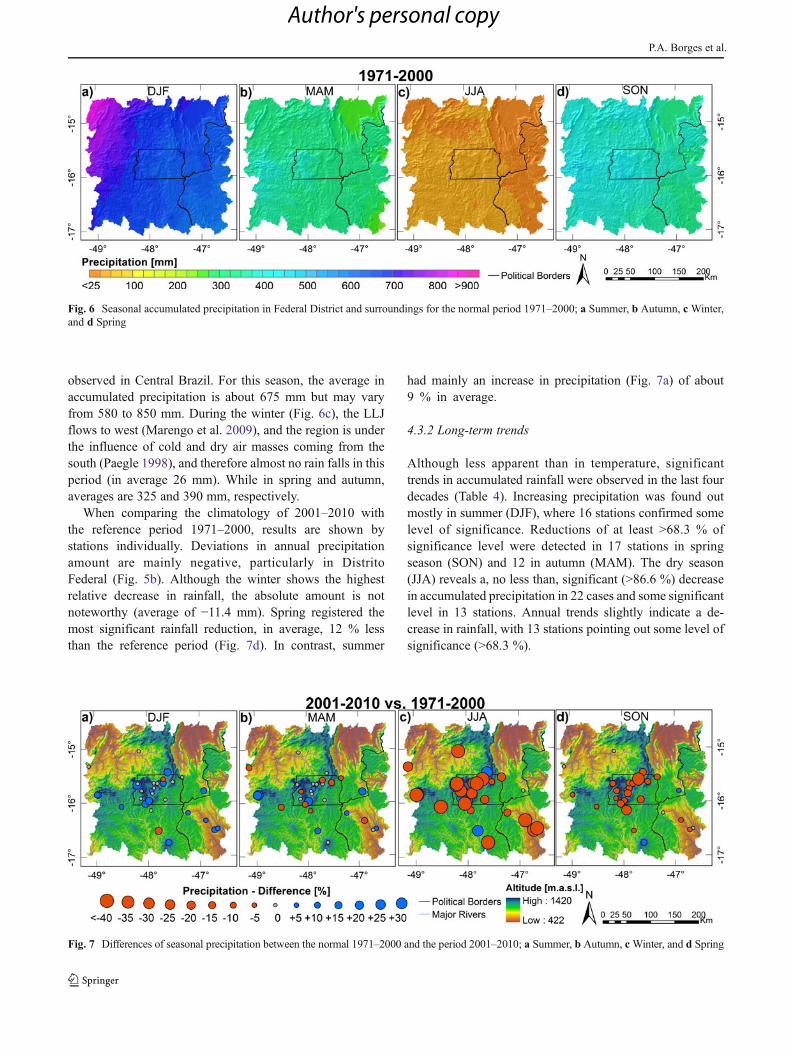
observed in Central Brazil. For this season, the average inaccumulated precipitation is about 675 mm but may varyfrom 580 to 850 mm. During the winter (Fig. 6c), the LLJflows to west (Marengo et al. 2009), and the region is underthe influence of cold and dry air masses coming from thesouth (Paegle 1998), and therefore almost no rain falls in thisperiod (in average 26 mm). While in spring and autumn,averages are 325 and 390 mm, respectively.

When comparing the climatology of 2001–2010 withthe reference period 1971–2000, results are shown bystations individually. Deviations in annual precipitationamount are mainly negative, particularly in DistritoFederal (Fig. 5b). Although the winter shows the highestrelative decrease in rainfall, the absolute amount is notnoteworthy (average of −11.4 mm). Spring registered themost significant rainfall reduction, in average, 12 % lessthan the reference period (Fig. 7d). In contrast, summer

had mainly an increase in precipitation (Fig. 7a) of about9 % in average.

4.3.2 Long-term trends

Although less apparent than in temperature, significanttrends in accumulated rainfall were observed in the last fourdecades (Table 4). Increasing precipitation was found outmostly in summer (DJF), where 16 stations confirmed somelevel of significance. Reductions of at least >68.3 % ofsignificance level were detected in 17 stations in springseason (SON) and 12 in autumn (MAM). The dry season(JJA) reveals a, no less than, significant (>86.6 %) decreasein accumulated precipitation in 22 cases and some significantlevel in 13 stations. Annual trends slightly indicate a de-crease in rainfall, with 13 stations pointing out some level ofsignificance (>68.3 %).

Fig. 6 Seasonal accumulated precipitation in Federal District and surroundings for the normal period 1971–2000; a Summer, b Autumn, c Winter,and d Spring

Fig. 7 Differences of seasonal precipitation between the normal 1971–2000 and the period 2001–2010; a Summer, b Autumn, cWinter, and d Spring

P.A. Borges et al.

Author's personal copy

Tab

le4

Trend

analysisof

season

alandannu

alprecipitatio

n

Statio

nID

DJF

MAM

JJA

SON

Ann

ual

Abs

(mm)

Rel(%

)SIG

(%)

Abs

(mm)

Rel(%

)SIG

(%)

Abs

(mm)

Rel(%

)SIG

(%)

Abs

(mm)

Rel(%

)SIG

(%)

Abs

(mm)

Rel(%

)SIG

(%)

0154

6000

46.12

7.64

NS

−37

.39

−14

.16

NS

−18

.46

−10

6.91

>95

.4−14

5.93

−43

.47

>90

−15

5.66

−12

.76

NS

0154

6005

b10

5.49

14.62

NS

74.33

21.07

NS

1.65

8.34

NS

38.29

10.01

NS

219.76

14.88

>68

.3

0154

7002

140.96

23.74

>90

−26

.05

−8.41

NS

1.9

8.24

>68

.3−12

8.95

−36

.86

>68

.3−12

.14

−0.95

NS

0154

7003

b−37

.18

−5.14

NS

−57

.63

−17

.54

NS

−6.59

−35

.42

NS

−30

.37

−8.57

NS

−13

1.77

−9.25

NS

0154

7004

−68

.87

−10

.41

NS

71.67

19.56

>68

.3−8.53

−24

.03

NS

−62

.22

−14

.14

NS

−67

.96

−4.52

NS

0154

7008

−43

.78

−7.47

NS

39.79

12.01

NS

−8.37

−35

.54

NS

−118.34

−28

.76

>68

.3−13

0.71

−9.67

NS

0154

7009

−73

.03

−12

.2NS

46.24

13.99

NS

3.52

13.33

NS

−82

.02

−20

.63

>68

.3−10

5.29

−7.78

NS

0154

7010

−4.09

−0.58

NS

−61

.93

−16

.12

NS

−5.01

−18

.27

NS

−10

1.76

−23

.41

NS

−17

2.79

−11.17

>68

.3

0154

7011

91.04

14.99

>80

3.39

1.05

NS

−5.39

−18

.11

>68

.3−47

.76

−12

.89

NS

41.28

3.1

NS

0154

7012

−9.68

−1.56

NS

−13

.85

−4.67

NS

−3.43

−13

.99

NS

−99

.3−25

.03

>68

.3−12

6.27

−9.43

NS

0154

7013

56.85

9.39

NS

−44

.41

−14

.33

NS

−5.21

−21

.79

>86

.6−62

.19

−16

.99

NS

−54

.96

−4.21

NS

0154

7014

a83

.93

12.73

NS

120.19

33.34

>68

.317

.24

64.6

NS

−65

.16

−15

.41

NS

156.19

10.63

NS

0154

7015

a−75

.36

−11.45

NS

−46

.85

−13

.53

NS

−10

.28

−38

.53

NS

−61

.29

−16

.14

NS

−19

3.77

−13

.73

>68

.3

0154

7016

b−23

6.11

−36

.27

>90

−40

.45

−14

.15

NS

−8.09

−33

.14

>68

.3−13

2.74

−38

.62

>86

.6−41

7.39

−31

.98

>95

.4

0154

8000

b49

.56.78

NS

−44

.84

−12

.2NS

−16

.81

−68

.95

>86

.6−31

.31

−7.64

NS

−43

.48

−2.84

NS

0154

8001

b−10

2.37

−15

.94

NS

−24

.22

−8.12

NS

−25

.62

−16

9.83

>99

−8.21

−2.3

NS

−16

0.41

−12

.23

>68

.3

0154

8003

133.46

16.93

>68

.310

3.54

26.96

>86

.6−13

.5−50

.23

NS

−65

.04

−15

.23

NS

158.46

9.74

>68

.3

0154

8004

156.75

19.2

>80

110.65

27.69

>95

−13

.3−45

.98

NS

−33

.01

−7.59

NS

221.09

13.16

>86

.6

0154

8005

149.28

20.55

>80

−49

.33

−13

.26

NS

−11.06

−33

.79

NS

−52

.76

−11.42

NS

36.13

2.27

NS

0154

8006

15.28

2.2

NS

−70

.28

−19

.43

>68

.3−10

.45

−37

.22

NS

−60

.86

−14

.39

NS

−12

6.31

−8.38

NS

0154

8007

52.03

7.34

NS

−30

.98

−8.2

NS

−38

.58

−118.08

>90

−62

.95

−15

.25

NS

−80

.48

−5.25

NS

0154

8014

199.14

28.29

>86

.665

.62

17.29

NS

9.04

29.68

NS

−26

.74

−6.12

NS

247.06

15.93

NS

0154

9000

22.12

2.97

NS

−10

2.64

−36

.49

>90

−13

.34

−73

.14

>86

.6−115

−29

.06

>95

.4−20

8.85

−14

.52

>80

0154

9001

−28

.27

−3.65

NS

−61

.91

−19

.16

>80

0.48

2.13

NS

−24

.64

−6.19

NS

−114.33

−7.53

NS

0154

9002

11.25

1.36

NS

−84

.57

−23

.29

>80

−17

.39

−74

.67

>95

−10

8.02

−26

.55

>86

.6−19

8.73

−12

.25

>80

0154

9003

90.67

10.32

>68

.3−10

1.09

−26

.9>86

.6−21

.43

−80

.54

>95

.4−10

8.09

−25

.29

>86

.6−13

9.94

−8.19

NS

0154

9004

b−11.38

−1.25

NS

−74

.78

−20

.06

>68

.3−20

.12

−93

.43

>95

−33

.58

−8.12

NS

−13

9.86

−8.13

NS

0154

9009

87.1

11.24

>68

.3−37

.63

−11.17

NS

−10

.39

−43

.24

>68

.3−52

.59

−13

.02

NS

−13

.51

−0.88

NS

0155

0000

b−44

.67

−5.46

NS

−43

.63

−13

.83

NS

−16

.47

−76

.78

>80

−28

.71

−7.77

NS

−13

3.47

−8.75

>68

.3

0155

0001

b−12

9.95

−13

.4NS

−14

5.61

−41

.29

>95

.4−10

.12

−53

.28

>86

.621

.07

5.19

NS

−26

4.6

−15

.15

>68

.3

0155

0002

b33

.43

4.21

NS

28.07

8.66

NS

−0.15

−1.11

NS

87.87

25.38

>80

149.22

10.1

>68

.3

0155

0003

123.89

13.1

NS

−48

.67

−12

.54

NS

0.53

2.13

NS

−17

.84

−4.07

NS

57.92

3.22

NS

0164

5000

113.98

21.38

>80

43.74

21.78

>68

.3−9.22

−77

.17

>95

.4−15

0.02

−52

.46

>95

.4−1.53

−0.15

NS

0164

5002

−90

.18

−18

.01

NS

−47

.4−23

.47

NS

−8.47

−65

.87

>99

.99

−17

4.1

−62

.59

>99

−32

0.15

−32

.22

>90

Differences between two climatological periods

Author's personal copy

Tab

le4

(con

tinued)

Statio

nID

DJF

MAM

JJA

SON

Ann

ual

Abs

(mm)

Rel(%

)SIG

(%)

Abs

(mm)

Rel(%

)SIG

(%)

Abs

(mm)

Rel(%

)SIG

(%)

Abs

(mm)

Rel(%

)SIG

(%)

Abs

(mm)

Rel(%

)SIG

(%)

0164

5003

67.75

12.46

>68

.3−42

.26

−20

.61

NS

−2.44

−17

.29

NS

−61

.7−21

.58

NS

−38

.64

−3.69

NS

0164

5005

−28

.47

−5.18

NS

−19

.81

−9.24

NS

−16

.71

−83

.52

>95

.4−59

.41

−19

.99

NS

−12

4.4

−11.5

NS

0164

5007

−2.26

−0.42

NS

−20

.54

−10

.59

NS

−4.63

−34

.32

>95

.4−13

2.8

−41

.08

>80

−16

0.23

−14

.97

NS

0164

5009

96.25

18.42

>68

.3−1.18

−0.59

NS

−6.76

−55

.65

NS

−70

.14

−25

.2NS

18.16

1.79

NS

0164

6000

147.86

25.52

>80

−5.78

−2.81

NS

1.48

7.66

NS

31.92

10.2

NS

175.48

15.7

>68

.3

0164

6001

53.09

8.42

>68

.3−55

.26

−18

.64

NS

−11.89

−58

.59

>86

.6−28

.92

−8.32

NS

−42

.98

−3.32

NS

0164

6003

104.65

16.46

NS

−28

.72

−9.82

NS

−11.67

−47

.27

>80

−35

.85

−11.1

NS

28.4

2.23

NS

0164

6004

b79

.69

13NS

17.36

6.01

NS

−14

.74

−85

.72

>68

.3−56

.01

−17

.18

NS

26.3

2.11

NS

0164

7001

150.44

22.33

NS

−4.87

−1.67

NS

−2.42

−11.76

NS

69.58

19.01

NS

212.73

15.73

NS

0164

7002

b28

5.21

39.86

>95

.430

.26

8.78

NS

−12

.07

−53

.17

NS

176.26

46.37

>95

.447

9.66

32.78

>95

.4

0164

7003

b−58

.13

−8.11

NS

−23

.98

−6.6

NS

−9.7

−32

.3NS

−37

.83

−10

.12

NS

−12

9.64

−8.74

NS

0164

7008

b−17

.36

−2.69

NS

−47

.75

−15

.35

NS

−5.87

−28

.23

>68

.318

.05

5.58

NS

−52

.92

−4.07

NS

0164

8001

57.63

8.33

NS

−64

.7−17

.68

NS

−15

.04

−56

.42

>90

−49

.93

−12

.44

NS

−72

.03

−4.85

NS

0164

9000

a14

9.81

22.41

>86

.6−8.21

−2.54

NS

−16

.96

−75

.62

>86

.6−72

.51

−19

.18

NS

52.13

3.74

NS

0164

9001

b−55

.52

−7.25

NS

18.58

5.16

NS

−14

.3−54

.69

>68

.3−13

.63

−3.47

NS

−64

.88

−4.2

NS

0164

9004

b−5.91

−0.82

NS

−24

.04

−6.64

NS

−20

.99

−94

.81

NS

40.43

10.08

NS

−10

.51

−0.7

NS

0164

9006

17.61

3.6

NS

−16

5.33

−54

.84

>99

−12

.13

−72

.08

>90

−16

4.27

−45

.23

>95

.4−32

4.11

−27

.69

>99

0164

9007

b35

.65

3.86

NS

−54

.89

−14

.92

>68

.3−17

.53

−84

.15

>99

44.39

9.69

NS

7.63

0.43

NS

0164

9009

b12

0.11

15.22

NS

−98

.92

−25

.03

>68

.3−11.22

−44

.14

>80

−18

6.17

−44

.74

>95

.4−17

6.19

−10

.84

>68

.3

0164

9010

16.41

2.53

NS

−36

.49

−12

.26

NS

−3.38

−15

.91

>68

.3−93

.03

−25

.09

NS

−116.48

−8.7

NS

0164

9012

b−26

7.02

−37

.03

>95

.4−18

2.65

−53

.57

>95

.4−23

.18

−87

.08

>86

.6−76

.03

−24

.61

>86

.6−54

8.89

−39

.27

>99

0164

9013

48.79

6.52

NS

28.32

7NS

−21

.89

−70

.25

>80

−60

.03

−13

.95

>68

.3−4.81

−0.3

NS

0165

0000

b10

3.5

13.86

>68

.3−80

.4−24

.19

NS

−12

.79

−52

.69

>68

.322

.42

6.37

NS

32.72

2.25

NS

0165

0001

b−32

6.6

−39

.77

>90

−23

3.62

−63

.73

>99

−17

.4−73

.38

>95

.4−17

0.42

−48

.27

>95

.4−74

8.03

−47

.81

>99

.9

0165

0002

b53

.23

6.19

NS

−63

.91

−18

.92

NS

−17

.49

−74

.13

>95

.4−48

.63

−12

.94

NS

−76

.8−4.81

NS

0165

0003

b−53

.61

−7.47

NS

−13

.27

−3.8

NS

−6.78

−26

.92

>68

.3−47

.26

−11.87

NS

−12

0.92

−8.11

NS

SIG

level;>86

.6%

=sign

ificant,>95

.4%

=very

sign

ificant,>99

.7%

=high

lysign

ificant,andNSno

tsignificant

(after

Schön

wiese

2000

).aCalculatio

nstartin

gfrom

01/12/19

72bCalculatio

nstartin

gfrom

01/12/19

73

P.A. Borges et al.

Author's personal copy

5 Conclusion

As frequency of data absence and network density play animportant role in the trustworthiness of the tests performed, acareful time series and spatial analysis of data quality is aprerequisite of any regional climate study. The tool used hereshows to be reliable in testing the homogeneity of climatetime series in the concerning region and could provide asatisfactory homogeneous database for performing climatol-ogy and trend analysis.

Maps using appropriated spatial interpolation techniquewere able to illustrate the spatial and temporal distribution oftemperature and rainfall over Federal District and surroundings,as well as the association of annual variability with tropical andextratropical atmospheric circulations. Comparisons betweentwo periods (i.e., 2001–2010 and 1971–2010) and analysis oflong-term trends of mean surface air temperature support thestatement that the region is already a subject of a recent climatewarming. Concerning the accumulated precipitation, the resultsof temporal variability demonstrated alterations in the seasonalrainfall rather than in the annual average. Decreases wereobserved mostly in winter and spring, while the summer facedan increase in precipitation amounts. Similarly, the long-termtrends analysis shows significant decrease in rainfall in winter,spring, and autumn; whereas in summer, trends were positive.Although beyond the topic addressed here, causes of thisregional phenomenon might be related to changes in land use,urbanization, or even global and local increase of anthropogen-ic emission of greenhouse gases.

In order to confirm significant precipitation variabilityover Federal District, we conclude that more detailed analy-sis is needed, for instance, statistical analysis of length andfrequency of dry/wet periods and extreme events. Moreover,other climate variables like relative humidity, solar radiation,and wind speed should be included.

Acknowledgments The author wishes to thank the International Wa-ter Research Alliance Saxony—IWAS initiative and the InternationalPostgraduate Studies in Water Technologies—IPSWaT scholarship pro-gram (both funded by the German Federal Ministry of Education andResearch, BMBF) for the opportunity given.

References

Aguilar E, Auer I, Brunet M, Peterson TC, Wieringa J (2003) Guidanceon metadata and homogenization. WMO TD N. 1186 (WCDMPN. 53), WMO, Geneva

Alexandersson H (1986) A homogeneity test to precipitation data. Int JClimatol 6:661–675

Alves LM (2009) Clima da Região Centro-Oeste do Brasil. In:Cavalcanti IFA, Ferreira NJ, Da Silva MGAJ, Silva Dias MAF(eds) Tempo e Clima no Brasil. Oficina de Textos, São Paulo, pp235–241

Bárdossy A, Pegram G (2011) Downscaling precipitation using region-al climate models and circulation patterns toward hydrology.Water Resour Res 47, W04505. doi:10.1029/2010WR009689

Bernhofer C (2004) Grundlagen der Meteorologie und Hydrologie.Script, Chair of Meteorology. TUD, Tharandt

Bernhofer C, Goldberg V, Franke J, Surke M, Adam J (2008a)REKLI—Sachsen-Anhalt II Regionale Klimadiagnose fürSachsen-Anhalt. Abschlussbericht zum Forschungsvorhaben desLandesamt für Umweltschutz. Sachsen-Anhalt, Dresden

Bernhofer C, Goldberg V, Franke J, Häntzschel J, Harmansa S, PluntkeT, Geidel K, Surke M, Prasse H, Freydank E, Hänsel S, MellentinU, Küchler W (2008b) Sachsen im Klimawandel, Eine Analyse.Sächsisches Staatsministerium für Umwelt und Landwirtschaft(Hrsg.), Dresden

BirsanM-V,Molnar P, Burlando P (2005) Streamflow trends in Switzerland.J Hydrol 314(1–4):312–329. doi:10.1016/j.jhydrol.2005.06.008

Borges P, Franke J, Tanaka M, Weiss H, Bernhofer C (2013) Spatialinterpolation of climatological information: comparison of methodsfor the development of precipitation distribution in Distrito Federal,Brazil. Atmos Clim Sci 3(2):208–217. doi:10.4236/acs.2013.32022

Buishand TA (1982) Some methods for testing the homogeneity ofrainfall records. J Hydrol 58(1-2):11–27. doi:10.1016/0022-1694(82)90066-X

Callejas IJA, de Oliveira AS, Santos FMD, Durante LC, NogueiraMCDA, Zeilhofer P (2011) Relationship between land use/coverand surface temperatures in the urban agglomeration of Cuiabá-Várzea Grande, Central Brazil. J App Remote Sens 5(1).doi:10.1117/1.3666044

Carvalho LMV, Jones C (2009) Zona de Convergência do Atlântico Sul.In: Cavalcanti IFA, Ferreira NJ, Da Silva MGAJ, Silva Dias MAF(eds) Tempo e Clima noBrasil. Oficina de Textos, São Paulo, pp 95–109

Carvalho LMV, Jones C, Liebmann B (2004) The South Atlanticconvergence zone: persistence, intensity, form, extreme precipita-tion and relationships with intraseasonal activity. J Climate 17:88–108

Craddock JM (1956) The representation of the annual temperature varia-tion over Central and northern Europe by a two-term harmonic form.Q.J.R. Meteorol Soc 82:275–288. doi:10.1002/qj.49708235304

Dahmen ER, Hall MJ (1990) Screening of Hydrological Data: Tests forStationarity and Relative Consistency. Publication No. 49,International Institute for Land Reclamation and Improvement(ILRI), Wageningen

Dixon WJ (1950) Analysis of extreme values. Ann Math Statist 21:488–506

Dobler C, Hagemann S, Wilby RL, Stötter J (2012) Quantifying differ-ent sources of uncertainty in hydrological projections in an Alpinewatershed. Hydrol Earth Syst Sci 16:4343–4360. doi:10.5194/hess-16-4343-2012

Dyras I, Dobesch H, Grueter E, Perdigao A, Tveito OE, Thornes JE,Fvd W, Bottai L (2005) The use of geographic information sys-tems in climatology and meteorology: COST 719. Met Apps,Brussels

Franke J, Goldberg V, Eichelmann U, Freydank E, Bernhofer C (2004)Statistical analysis of regional climate trends in Saxony, Germany.Clim Res 27:145–150

Gan MA, Kousky VE, Ropelewski CF (2004) The South Americamonsoon circulation and its relationship to rainfall over West-Central Brazil. J Climate 17:47–66. doi:10.1175/1520-0442(2004)017<0047:TSAMCA>2.0.CO;2

Helsel DR, Hirsch RM (2002) Statistical methods in water resourcestechniques of water resources investigations. U.S. GeologicalSurvey, USA

Herzog J, Müller-Westermeier G (1998) Homogenitätsprüfung undHomogenisierung klimatologischer Messreihen im DeutschenWetterdienst. Deutsch Wetterdienst, Offenbach

Differences between two climatological periods

Author's personal copy

IPCC-TGCIA (1999) Guidelines on the Use of Scenario Data forClimate Impact and Adaptation Assessment. Version 1. Preparedby Carter, T.R., M. Hulme, and M. Lal. Intergovernmental Panelon Climate Change, Task Group on Scenarios for Climate ImpactAssessment, Geneva

Karpouzos DK, Kavalieratou S, Babajimopoulos C (2010) Trend anal-ysis of precipitation data in Pieria Region (Greece). EuropeanWater 30:31–40

Kendall MG (1970) Rank correlation methods, 4th edn. Griffin,London

Kousky VE (1988) Pentad outgoing longwave radiation climatology forthe South American sector. Rev Brasileira de Meteorologia 3:217–231

Lhotellier R (2005) Spatialisation des températures en zone demontagne alpine. Université Joseph Fourier, Dissertation

Lorz C, Abbt-Braun G, Bakker F, Borges P, Börnick H, Fortes L,Frimmel F, Gaffron A, Hebben N, Höfer R, Makeschin F, NederK, Roig HL, Steiniger B, StrauchM,Walde DH,Weiß H,Worch E,Wummel J (2012) Challenges of an integrated water resourcemanagement for the Distrito Federal, Western Central Brazil:climate, land-use, and water resources. Environ Earth Sci65(5):1363–1366. doi:10.1007/s12665-011-1219-1

Lu X (2006) Guidance on the Development of Regional ClimateScenarios for Application in Climate Change Vulnerability andAdaptation Assessments. Within the Framework of NationalCommunications from Parties not Included in Annex I to theUnited Nations Framework Convention on Climate Change,National Communications Support Program. UNDP-UNEP-GEF,New York

Maddox RA (1980) Mesoscale convective complexes. Bull AmMeteorol Soc 61:1374–1387. doi:10.1175/1520-0477(1980)061<1374:MCC>2.0.CO;2

Mann HB (1945) Nonparametric test against trends. Econometrica13(3):245–259

Marengo JA, Ambrizzi T, Soares WR (2009) Jatos de Baixos Níveis aolongo dos Andes. In: Cavalcanti IFA, Ferreira NJ, Da Silva MGAJ,Silva Dias MAF (eds) Tempo e Clima no Brasil. Oficina de Textos,São Paulo, pp 169–180

Martínez MD, Serra C, Burgueño A, Lana X (2009) Time trends ofdaily maximum and minimum temperatures in Catatonia (NESpain) for the period 1975–2004. Int J Climatol 30(2):267–290.doi:10.1002/joc.1884

Nalder IA, Wein RW (1998) Spatial interpolation of climatic normals:test of a new method in the Canadian boreal forest. Agric Meteorol92:211–225

Nash JE, Sutcliffe JV (1970) River flow forecasting through conceptualmodels part I – A discussion of principles. J Hydrol 10(39):282–290. doi:10.1016/0022-1694(70)90255-6

Paegle J (1998) A comparative review of South American low level jets.Meteorologica 3:73–82

Pavlik D, Söhl D, Pluntke T, Mykhnovych A, Bernhofer C (2012)Dynamic downscaling of global climate projections for easternEurope with a horizontal resolution of 7 km. Environ. Earth Sci65:1475–1482. doi:10.1007/s12665-011-1081-1

Rapp J (2000) Konzeption, Problematik und Ergebnisse klimatologischerTrendanalysen für Europa und Deutschland. Bericht Nr.212,Deutsch Wetterdienst, Offenbach

Rapp J, Schönwiese CD (1995) Klimatrend-Atlas Deutschland 1891–1990. Frankfurt Geowiss Arb 5, University of Frankfurt (Main)

Renard F, Comby J (2006) Evaluation of rainfall spatial interpolationmethods in urban area for a better management of extreme rainyevents: the case of the urban area of Greater Lyon. Le HouileBlanche 6:75–78. doi:10.1051/lhb:2006104

Salas D (1993) Analysis and modeling of hydrologic time series(Chapter 19). In: Maidment DR (ed) Handbook of Hydrology.McGraw Hill, New York

Schönwiese CD (2000) Praktische Statistik für Meteorologen undGeowissenschaftler. Gebrüder Borntaeger 3, Berlin

Schönwiese CD,Malcher J (1985) Nicht Stationarität oder Inhomogenität?Ein Beitrag zur statistischen Analyse klimatologischer Zeitreihen.Wetter Leben 37:181–193

Trewin B (2007) The role of climatological normals in a changingclimate Tech. Rep. WDMCP-No. 61 World MeteorologicalOrganization, Geneva

Tveito OE, Førland EJ (1999) Mapping temperatures in Norway apply-ing terrain information, geostatistics, and GIS. Norsk geogrTidsskr 53:202–212. doi:10.1080/002919599420794

Vera C, Higgins W, Amador J, Ambrizzi T, Garreaud R, Gochis D,Gutzler D, Lettenmaier D, Marengo J, Mechoso CR, Nogues-Paegle J, Silva Diaz PL, Zhang C (2006) Towards a unified viewof the American monsoon system. J Climate 19:4977–5000

Wackernagel H (2003) Multivariate Geostatistics. Springer, BerlinWilby R, Dawson CW (2012) The statistical downscalingmodel: insights

from one decade of application. Int J Climatol. doi:10.1002/joc.3544WMO (1989) World Climate Data Program: Calculation of Monthly

and Annual 30-year Standard Normals, WCDP-No.10, WMO-TD/No. 341, Prepared by a meeting of experts, Washington

Zhou J, Lau KM (1998) Does a Monsoon Climate Exist over SouthAmerica? J Climate 11:1020–1040. doi:10.1175/1520-0442(1998)011<1020:DAMCEO>2.0.CO;2

P.A. Borges et al.

Author's personal copy