(0206) FACULTY NAME: Mr. Mukesh Kumar Assistant

DARBHANGA COLLEGE OF ENGINEERING

COURSE FILE

OF

_____ENGINEERING MATERIAL ______

(0206)

FACULTY NAME:

Mr. Mukesh Kumar

Assistant Professor

DEPARTMENT OF Mechanical engineering

Time/Day MONDAY TUESDAY WEDNESDAY

THURSDAY FRIDAY SATURDAY

9:00am- 10:00am

ENGINEERING MATERIAL

10:00am-11:am

INDUSTRIALPOLLUTION(IP)

INDUSTRIALPOLLUTION

(IP)


ENGINEERINGMATERIAL(T)

11:00am-12:00pm

ENGINEERINGMATERIAL

INDUSTRIALPOLLUTION

(IP)

12:00pm-01:00pm

INDUSTRIALPOLLUTION

IP(T)

INDUSTRIALPOLLUTION

IP(T)

1:00pm-2:00pm

LUNCH

2:00PM-3:00PM

WORKSHOP WORKSHOP WORKSHOP WORKSHOP3:00PM-4:00PM

4:00PM-5:00PM

TIME TABLE

FACULTY NAME: Mr. Mukesh kumar

MECHANICAL ENGINEERING DEPARTMENT

VISION

To bring forth quality engineers embodying societal ethics to serve national and multinational

organisations as well as harping on higher studies.

MISSION

1. To create a modern teaching-learning ambience focusing on advanced pedagogy and tools for mechanical engineers

2. To collaborate with domain industry and research institutes to enhance the skills and knowledge of the graduates.

3. To inject necessary professional skills to serve the industry and the nation4. To inculcate humanitarian ethical values in graduates through various social-cultural activities

Program educational objectives(PEO’s)

1. The graduates will be able to demonstrate the knowledge and skills of mechanical engineeringto obtain solutions to engineering problems.

2. The graduates will be able to apply mechanical engineering concepts while pursuingacademic and research activities.

3. The graduates will be able to showcase professional skill and expertise.

Program specific outcomes(PSOs)

1. Students should be oriented towards research in engineering technologies like Advancemanufacturing, 3D Printing, Alternative fuels to contribute the evolving research anddevelopment in the field of Mechanical Engineering.

2. Students should be able to learn and apply software like AutoCAD, Ansys, Catia for variousapplications.

SYLLABUS

B. Tech. 3rd Semester (MECHANICAL)ME- 0206 Engineering Material

L T P/D Total Max Marks: 100 3-1-0 4 Final Exams: 70 Marks

Internals: 30 Marks

UNIT-I

Crystal Structure: Unit cells, Metallic crystal structures, Ceramics. Imperfection in solids: Point, line,

interfacial and volume defects; dislocation strengthening mechanisms and slip systems, critically

resolved shear stress.

UNIT-II

Alloys, substitutional and interstitial solid solutions- Phase diagrams: Interpretation of binary phasediagrams and microstructure development; eutectic, peritectic, peritectoid and monotectic reactions.Iron Iron-carbide phase diagram and microstrctural aspects of ledeburite, austenite, ferrite andcementite, cast iron.

UNIT-III

Mechanical Property measurement: Tensile, compression and torsion tests; Young’s modulus,relations between true and engineering stress-strain curves, generalized Hooke’s law, yielding andyield strength, ductility, resilience, toughness and elastic recovery; Hardness: Rockwell, Brinell andVickers and their relation to strength, Introduction to non-destructive testing (NDT).

UNIT-IV

Heat treatment of Steel: Annealing, tempering, normalising and spheroidising, isothermal

transformation diagrams for Fe-C alloys and microstructure development. Continuous cooling curves,

T-T-T diagram and interpretation of final microstructures and properties- austempering, martempering,

case hardening, carburizing, nitriding, cyaniding, carbo-nitriding, flame and induction hardening,

vacuum and plasma hardening.

UNIT-V

Alloying of steel, properties of stainless steel and tool steels, maraging steels- cast irons; grey, white,malleable and spheroidal cast irons- copper and copper alloys; brass, bronze and cupronickel;Aluminium and Al-Cu – Mg alloys- Nickel based superalloys and Titanium alloys.

Books:1. Material Science and Engineering: An Introduction by William D Callistor,

2. Material Science and Engineering: An Introduction by V. Raghavn

COURSE HANDOUT

Institute / College Name : Darbhanga College of EngineeringProgram Name B.Tech Mechanical EngineeringCourse Code ME0206Course Name Engineering MaterialLecture / Lab (per week): 3/0 Course Credits 4Course Coordinator Name MR. Mukesh Kumar

Course Description

The course is designed to provide a basic understanding of science behind materials. Introduce the

concept of structure property relations. Lay the groundwork for studies in fields such as solid-state

physics, mechanical behavior of materials, phase & phase diagram, heat treatment, failure of

materials & their protection, applications of Recent materials. Through lectures, demonstrations, and

firsthand laboratory exposure, the student is given the theory and applications of different materials.

The following are covered: engineering materials, iron carbon system, phase and phase diagram, heat

treatment, cast iron, composite materials.

Course Objectives

1. To expose the students to a variety of materials with comparable properties including theirapplications.

2. To teach the crystal structure, crystal imperfections and important effects.3. To teach behaviour of iron and iron carbon equilibrium diagram.4. To study different phase and phase diagram.5. Explain the different types of heat treatment (TTT & CCT) Process.6. To teach properties and types of composites materials.

Course Outcomes

1. Analyze the Structure of materials at different levels, basic concepts of crystalline materials like

unit cell, FCC, BCC, HCP, APF (Atomic Packing Factor), Co-ordination Number etc.

2. Understand concept of mechanical behavior of materials and calculations of same using

appropriate equations.

3. Explain the concept of phase & phase diagram & understand the basic terminologies associated

with metallurgy. Construction and identification of phase diagrams and reactions.

4. Understand and suggest the heat treatment process & types. Significance of properties Vs

microstructure. Surface hardening & its types. Introduce the concept of hardenability &

demonstrate the test used to find hardenability of steels.

5. Explain features, classification, applications of composite materials and influence of fiber

orientation.

DARBHANGA COLLEGE OF ENGINEERING, DARBHANGA


SEMESTER: 4th A.Y. - 2020

SUBJECT: Engineering Material

SUBJECT CODE: 0206

ASSIGNMENTS

SR.

NO.QUESTIONS

CHAPTER 1- Introduction to Material Science

1. Explain the structure-property-performance relationship with suitable example.

2. Explain the requirement of engineering materials.

3. Classify the engineering materials. Explain any two of them.

4. Explain Criteria for Selection of Engineering Material

CHAPTER 2 - Crystal geometry and Crystal Imperfections

5. Differentiate between Edge and Screw dislocation with sketch.

6. Explain imperfections in crystal with neat sketches.

7. Draw a unit cell and show the following planes (a) (113) (b) (102) (c) (111) and (d) (001).

8.What is critical nucleus? In case of crystallization of metals, what is the difference between an embryo and a nucleus? What is the significance of critical radius of a solidifying particle?

9.Explain with neat sketches the arrangement of atoms, in S.C, B.C.C, F.C.C. and H.C.P. lattice. And Also write Effective Number of atom, Atomic Packing Factor, Co-ordination Number for all Lattices. Define unit cell.

10. What are the various levels of structure? Explain in detail

CHAPTER 3- Phase and Phase equilibrium

11.What is Gibb’s phase rule? Calculate the degree of freedom, for eutectic composition in binary phase diagram.

12.Draw the phase diagram of isomorphous system of binary alloy A and B. explain the equilibriumcooling of 30A-70B composition from liquid to solid state (up to room temperature).

13. Explain the “Hune-Rothery Rules” for solid solution, with suitable case study.

14.Compare cooling curves for pure metal, isomorphous and non-isomorphous alloys. State the information revealed by these cooling curves.

15. Explain substitutional and interstitial solid solution.

16. What is phase diagram? Explain Lever rule.

17. Explain thermal equilibrium diagram of binary alloys.

18.Derive the lever rule for the amount in wt. percent of each phase in two phase regions of binary phase diagram.

19.

Bismuth(Bi) and cadmium(Cd) with melting points of 270 and 320 respectively are incomplete solubility in solid state. They form a eutectic of composition 40% Bi at 145 temperatures.Find a) an alloy containing 80% Bi, sketch the corresponding cooling curve taking necessary points from the phase diagram.b)calculate the amount of proeutectic & eutectic constituents obtained upon slow cooling temperature for this alloy.

20.Calculate the percentage of ferrite, carbide and pearlite at room temperature in iron-iron carbide diagram for the alloy containing:a).5% carbon b) .8% carbon c) 1.5percent carbon

CHAPTER 4- Iron-Iron-Carbide equilibrium system

21. Explain the allotropic behaviour of Iron with sketch.

22. Draw and explain microstructure of eutectoid steel.

23.Draw iron – iron carbide equilibrium diagram. Explain important phases in it. Discuss the phase transformation takes place for the 0.6 % carbon steel from liquid to room

24.Draw iron – iron carbide equilibrium diagram with all necessary details. Briefly explain cooling of 1.2 % carbon steel from liquid state to room temperature.

25. Draw microstructure of (i) 04 % carbon steel and (ii) eutectoid steel at room temperature.

CHAPTER5- CAST IRON

26.State composition, specific properties and applications of Grey Cast Iron

27.Differentiate between white cast iron and grey cast iron

28.Classify different types of cast iron. Why silicon is added to cast iron? Explain the effects of any four alloying elements on the properties of cast iron

29. Explain the graphitization process. Also enlist the factors affecting the graphitization in cast iron.

CHAPTER 6- HEAT TREATMENT OF STEELS

30. Explain tempering and compare austempering and martempering.

31.Why is heat treatment needed? Compare annealing and normalizing

Process as regards to their objectives, applications, process limitations and process merits.32. Differentiate flame hardening and induction hardening process on the basis of parametric

control, process features, operational safety and productivity.

33.Compare and contrast carburizing and nitriding process with reference to parametric controls,

process features, process limitations and applications.

34.

Compare the hardenability curves obtained from Jominy endquench test for plain carbon steels

with hypoeutectoid and hypereutectoid composition and comment on the hardenability of these

two steels.

35. Draw TTT diagram for eutectoid steel. Explain briefly by cooling few cooling rates.

36.

What is the purpose of heat treatment? Differentiate Annealing and Normalizing on the basis

of : (I) Rate of cooling (II) Microstructure after cooling (III) Grain size distribution (IV)

Internal Stresses (V) Mechanical properties (VI) Application

37.Explain the effects of grain size, heat treatment and alloying elements on properties of single

phase material

CHAPTER 7 COMPOSITES

38.

Derive the rule of mixture for calculating Young's Modulus of an aligned fiber reinforced

composite loaded parallel to the direction of fiber orientation and perpendicular to fiber

alignment.

39. Explain difference between fibers and whiskers?

40. Define composite material. Give examples use of composite materials

41. What are hybrid composites? Give one example.

42.

A continuous and aligned fiber-reinforced composite is to be produced consisting of 30 vol%

aramid fibers in polycarbonate matrix. Mechanical properties are as follows: modulus of

elasticity for aramid fiber = 131 GPa modulus of elasticity for polycarbonate = 2.4 GPa

Assume that the composite has a cross-sectional area of 320 mm2 and is subjected to a

longitudinal load of 44500 N. Calculate:

1.The fiber-matrix load ratio

2.The actual loads carried by both fiber and matrix

3.The magnitude of the stress on each of the fiber and matrix

4.What strain is experienced by the composite?

43. Write short notes on GFRP,CFRC,AFRC.

TUTORIAL-I

Give the answer of following questions:Choose one of the correct options for following questions

1. Gibbs phase rule for general system: a) P+F=C-1 b) P+F=C+1c) P+F=C-2 d) P+F=C+2

2. Above the following line, liquid phase exists for all compositions in a phase diagram. a) Tie-line b) Solvus c) Solidus d) Liquidus

3. Following is wrong about a phase diagram. a) It gives information on transformation rates. b) Relative amount of different phases can be found under given equilibrium

conditions. c) It indicates the temperature at which different phases start to melt. d) Solid solubility limits are depicted by it.

4. The boundary line between (alpha) and (alpha+beta) regions must be part of a) Solvus b) Solidus c) Liquidusd) Tie-line

5. An invariant reaction that produces a solid up on cooling two liquids: a) 0 b) 1 c) 2 d) 3

6. In a single-component condensed system, if degree of freedom is zero, maximum number of phases that can co-exist _________ a) Eutecticb) Peritecticc) Monotecticd) Syntectic

7. Classify engineering materials. Explain any two of them with examples

8. Bismuth (Bi) and Antimony are completely soluble in both liquid and solidstates. Bismuth melts at 270°C and antimony at 630°C.An alloy containing50% Bi starts to solidify at 505°C by separating crystals of 90%Sb. An alloycontaining 80%Bi starts to solidify at 400°C by separating crystals of 75% Sb.a) Draw the equilibrium phase diagram for the system and level all points,

lines and phase fields.b) For an alloy containing 40%Sb, find the phases present at 400°C and draw

the cooling curve for the same alloy.

TUTORIAL-II

1. The eutectic mixture of austenite (γ) and cementite (Fe3C) is called

a) Ledeburite b) Pearlite c) Hyper and hypo eutectoid steel d) Cast

iron

2. Compositions right and left of 0.8% C of Pearlite are called

a) Ledeburite b) Ferrit c) Hyper and Hypo eutectoid steel

d) Cast iron

3. What is Eutectic reaction at 1146°C?

a) L (0.53% C) + δ(0.09% C) → γ(0.17% C)

b) L (4.3% C) → γ(2.1 % C) + Fe3C (6.67% C)

c) γ (0.8 % C) → α (0.025% C) + Fe3C (6.67% C)

d) L (0.53% C) + δ(0.09% C) → γ (0.8 % C)

4. Compositions above 2.1% C is called as

a) Ledeburite b) Ferrite c) Hyper and Hypo eutectoid steel d) Cast

iron

5. Silicon percentage in white cast iron is

a) <1% b) 1-3% c) >1% d) none of these

6. A eutectoid steel is slowly cooled from temperature of 750°C to a temperature just

below 727°C. Calculate the percentage of ferrite and cementite.

TUTORIAL-III

Give the answer of the following questions:

1. Explain the annealing and normalizing heat treatment process

2. Gove the difference between Pearlite & Bainite structure of steel

3. Explain TTT Diagram

4. What is tempering and why it is required

TUTORIAL-IV

Write the answer of the following question:

1. Draw iron – iron carbide equilibrium diagram and write the reactions involve in it.

2. Explain the microstructure of hypoeutetoid steel containing 0.6% carbon

3. Differentiate between gray cast iron (G.C.I) and white cast iron (W.C.I)

TUTORIAL-V

Write the Answers of following questions:

1. Explain Austempering and Martempering.

2. Give the difference between Fiber and Whisker.

3. What is structural composites?

4. Give the difference between Fiber and Matrix.

5. Find modulus of elasticity of transverse Fiber composites.

MID SEMESTER QUESTION PAPER

Enroll. No. _____________


B. Tech – SEMESTER-III • MID SEMESTER- EXAMINATION

SUBJECT: MATERIAL SCIENCE (021305)

DATE: 05-04-2019 TIME: 11:00 am to 01:00 pm TOTAL MARKS: 20

Instructions: 1. All the questions are compulsory.

2. Figures to the right indicate full marks. 3. Assume suitable data if required.

Q.1 (a) Platinum (Pt) and Gold(Au) with melting points of 1775°C and 1062°C respectively

are complete solubility in liquid & solid state. An alloy containing 70% gold starts

to solidify at 1385°C by separating crystals of 37% gold. Determine the relative

amounts of solid and liquid phases of an alloy containing 50% gold at 1385°C.

[05]

(b) Explain the allotropic transformation of iron with neat sketch. [02]

Q.2 (a) Classify different types of material with their properties and applications. [02]

(b) Draw iron carbon equilibrium diagram and write the reactions involve in it. [05]

OR

Q.2 (a) What is solid solution? Explain the Hume Rothery’s rule for the formation of

substitutional solid solution with examples. [02]

(b) A continuous and aligned fiber-reinforced composite is to be produced consisting of

30 vol% aramid fibers in polycarbonate matrix. Mechanical properties are as

follows: modulus of elasticity for aramid fiber = 131 GPa modulus of elasticity for

polycarbonate = 2.4 GPa.Assume that the composite has a cross-sectional area of

320 mm2 and is subjected to a longitudinal load of 44500 N. Calculate:

a) The actual loads carried by both fiber and matrix.

b) The magnitude of the stress on each of the fiber and matrix.

[05]

Q.3 (a) Derive the rule of mixture for calculating Young's Modulus of an aligned fiber

reinforced composite loaded parallel to the direction of fiber orientation and

perpendicular to fiber alignment.

[04]

(b) Differentiate between white cast iron and gray cast iron in respect of microstructure,

composition and mechanical properties. [02]

OR

Q.3 (a) Define heat treatment. Draw TTT diagram for eutectoid steel. Explain briefly by

cooling few cooling rates. [04]

(b) Derive the lever rule for the amount in wt. percent of each phase in two phase

regions of a binary phase diagram. [02]

Enroll. No. _____________


B.Tech – SEMESTER-IV • MID SEMESTER- EXAMINATION

SUBJECT: ENGINEERING MATERIALS (ME)

DATE: 19-03-2020 TIME: 11:00 AM to 01:00 PM TOTAL MARKS: 20

Instructions: 1. All the questions are compulsory.

2. Figures to the right indicate full marks. 3. Assume suitable data if required.

Q.1 Define dislocation and differentiate between edge dislocation and screw

dislocation with neat sketch.

[04]

Q.2 Define the following terms

1. unit cell,

2.coordination number

3. Grain boundary

4. Atomic packing fraction

[03]

Q.3 Enlist and explain various point defects.

[03]

Q.4 State the types of solid solution and explain Hume Rothery’s rule for the

formation of solid solution.

[03]

Q.5 Sketch within the unit cubic cell the following planes.

1. (101) 2. (001) 3. (010) 4. (110)

[03]

Q.6 What is critical resolved shear stress and derive the equation of it. [04]

DARBHANGA COLLEGE OF ENGINEERING, DARBHANGA


Subject: Engineering Material

Name of Faculty Mr. Mukesh kumar

Semester: 4th

Subject code: 0206

QUESTION BANK

SR.

NO.QUESTIONS

UNIT 1

1. Differentiate between Edge and Screw dislocation with sketch.

2. Explain imperfections in crystal with neat sketches.

3. Draw a unit cell and show the following planes (a) (113) (b) (102) (c) (111) and (d) (001).

4.Explain with neat sketches the arrangement of atoms, in S.C, B.C.C, F.C.C. and H.C.P. lattice. And Also write Effective Number of atom, Atomic Packing Factor, Co-ordination Number for all Lattices. Define unit cell.

5. What are the various levels of structure? Explain in detail

6. Define critical resolved shear stress and derive the equation of same

7. Differentiate between slip and twinning.

8. Enlist various surface defects & explain any two of them.

9. What are the various strengthening mechanism for materials.? Explain any two of them.

10. Derive Schmid’s law wih usual notations.

11. Why FCC metals are more ductile as compared to BCC Metals. Explain it.?

12.What are the slip bands and slip lines.? Draw required sketches. What causes the formation of such bands on a metal surface.

13. Mention the significance of dislocations.

14. Define grain boundary and justify grain boundary is a surface imperfection.

15. State the difference between a space lattice and crystal structure.

16.

A single crystal of aluminium is oriented for tensile test such that its slip plane normal makes an angle of 28.1° with the tensile axis. three possible slip directions make an angles of 62.4°, 72°, and 81.1° with the same tensile axis.

(1) Which of these three slips is most favoured.(2) If plastic deformation begins at a stress of 1.95MPa, determine the critical resolved shear

stress for this crystal.

17. What is burger vector and explain its significance.

18. Edge dislocations result into generation of stress field around dislocation. justify it.?

19. What is plastic deformation.? Explain the mechanism of plastic deformation.

20. What is small angle boundaries(tilt boundaries) and high angle grain boundaries.?

21.

Iron is(a) paramagnetic(b) ferromagnetic(c) ferroelectric(d) dielectric

22.

A specimen of aluminium metal when observed under microscope shows(a) B.C.C. crystalline structure(b) F.C.C. crystal structure(c) H.C.P. structure(d) a complex cubic structure

23.

Body centered cubic structure has an atomic packing factor equal toa. 0.74b. 0.68c. 0.52d. None of the above

24.

In which type of point defect, positive and negative ions are missing from the crystal?a. Vacancy defectb. Interstitial defectc. Schottky defectd. Substitutional defect

25.

What is meant by Frenkel defect?a. defect in which interstitial position is occupied by missing atomsb. defect in which positive and negative ions are missingc. defect in which interstitial position is occupied by extra atom in the crystal without disorganizing the parent atomd. none of the above

UNIT 2

26. What is an alloy? What is the importance of forming alloys.?

27. How are alloys classified.?

28. Draw the cooling curve of pure metal and alloy.

29. What is solid solution.? Explain types of solid solution.

30. Differentiate between interstitial and substitution solid solution.

31. Explain the allotropic behaviour of Iron with sketch.

32. Draw and explain microstructure of eutectoid steel.

33.Draw iron – iron carbide equilibrium diagram. Explain important phases in it. Discuss the phase transformation takes place for the 0.6 % carbon steel from liquid to room temperature.

34.Draw iron – iron carbide equilibrium diagram with all necessary details. Briefly explain cooling of 1.2 % carbon steel from liquid state to room temperature.

35.What is Gibb’s phase rule? Calculate the degree of freedom, for eutectic composition in binary phase diagram.

36.Draw the phase diagram of isomorphous system of binary alloy A and B. explain the equilibriumcooling of 30A-70B composition from liquid to solid state (up to room temperature).

37. Explain the “Hume-Rothery Rules” for solid solution, with suitable case study.

38.Compare cooling curves for pure metal, isomorphous and non-isomorphous alloys. State the information revealed by these cooling curves.

39. Explain substitutional and interstitial solid solution.

40. What is phase diagram? Explain Lever rule.

41. Explain thermal equilibrium diagram of binary alloys.

42.Derive the lever rule for the amount in wt. percent of each phase in two phase regions of binary phase diagram.

43.

Bismuth(Bi) and cadmium(Cd) with melting points of 270 and 320 respectively are incomplete solubility in solid state. They form a eutectic of composition 40% Bi at 145 temperatures.Find a) an alloy containing 80% Bi, sketch the corresponding cooling curve taking necessary points from the phase diagram.b)calculate the amount of proeutectic & eutectic constituents obtained upon slow cooling temperature for this alloy.

44.Calculate the percentage of ferrite, carbide and pearlite at room temperature in iron-iron carbide diagram for the alloy containing:a).5% carbon b) .8% carbon c) 1.5percent carbon

45. Draw microstructure of (i) 04 % carbon steel and (ii) eutectoid steel at room temperature.

46.

Mild steel is an alloy of iron and carbon with percentage of carbon ranging from(a) up to 0.2%(b) 0.15–0.3(c) 0.3–0.5(d) above 0.5.

47.

The strength of steel increases with increasing carbon %age in the range(a) 0–0.8%(b) 0.8–1.2%(c) 1.2–2%(d) all of these ranges.

48.

Railway rails are normally made of(a) mild steel(b) alloy steel(c) high carbon(d) tungsten steel

49.

Eutectoid steel contains following percentage of carbon(a) 0.02%(b) 0.3%(c) 0.63%(d) 0.8%

50.

Maximum percentage of carbon in ferrite is(a) 0.025%(b) 0.06%(c) 0.1%(d) 0.25%

UNIT 3

51. Define the terms brittleness and hardness.

52. What do you mean by toughness and stiffness?

53. Explain in detail Creep and resilience.

54. Differentiate between brittle and ductile fracture.

55. Describe a Brinell hardness test to determine the hardness of a metal.

56. Explain the procedure for performing the Rockwell test.

57. Explain the Izod test and charpy test to determine the impact strength of a material.

58. Describe A Tensile Test To Determine Various Tensile Properties

59. Explain The Testing Procedure Of (i) A Compression Test, And (ii) A Shear Test

60.Draw engineering stress – strain curve for mild steel, aluminium and cast iron. Discuss the tensile test and different mechanical properties obtained in tensile test.

61. Differentiate between engineering stress and true stress.

62. Derive the relationship between engineering stress and strain.

63. Derive the relationship between engineering stress and strain.

64.The ultimate tensile strength of a material is 400MPa and elongation up to maximum load is 35%. If the material obeys power law, then what will be the true stress-strain relationship. given n=€=0.3

65. Compare destructive and non-destructive testing stating benefits & limitations.

66. State the principle of magnetic particle testing and enumerates the steps for it.

67. Explain the principle of ultrasonic testing and states various inspection technique used.

68. Write the advantage and limitations of ultrasonic testing.

69. Explain liquid penetration testing (Dye Penetration testing) method.

70. Explain radiography testing method for detecting defects in metal.

71.

IZOD test measures(a) hardness(b) ductility(c) impact-strength(d) grain size.

72.

Which test measures hardness?(a) Brinell test(b) Rockwell test(c) Vicker’s test(d) All of these tests.

73.

Ductility of a material can be defined as(a) ability to undergo large permanent deformations in compression(b) ability to recover its original form(c) ability to undergo large permanent deformations in tension(d) all of the above

74.

Malleability of a material can be defined as(a) ability to undergo large permanent deformations in compression(b) ability to recover its original form(c) ability to undergo large permanent deformations in tension(d) all of the above

75.

Austenite rs a combination of(a) ferrite and cementite(b) cementite and gamma iron(c) ferrite and austenite(d) ferrite and iron graphite

UNIT 4

76. What is heat treatment of steel.? What is its objective?

77. Explain tempering and compare austempering and martempering.

78.Why is heat treatment needed? Compare annealing and normalizing process as regards to their

objectives, applications, process limitations and process merits.

79.Differentiate flame hardening and induction hardening process on the basis of parametric

control, process features, operational safety and productivity.

80.Compare and contrast carburizing and nitriding process with reference to parametric controls,

process features, process limitations and applications.

81.

Compare the hardenability curves obtained from Jominy endquench test for plain carbon steels

with hypoeutectoid and hypereutectoid composition and comment on the hardenability of these

two steels.

82. Draw TTT diagram for eutectoid steel. Explain briefly by cooling few cooling rates.

83.

What is the purpose of heat treatment? Differentiate Annealing and Normalizing on the basis

of : (I) Rate of cooling (II) Microstructure after cooling (III) Grain size distribution (IV)

Internal Stresses (V) Mechanical properties (VI) Application

84.Explain the effects of grain size, heat treatment and alloying elements on properties of single

phase material

85.Differentiate between Continuous cooling Transformation (CCT) and time temperature

transformation (TTT).

86.Explain The Following Case Hardening Process Briefly with Neat Sketch.

A. Carburising B. Nitriding C. Cyaniding D. Carbonitriding

87.Compare And Contrast The Process Of Full Annealing, Process Annealing, Stress Relief

Annealing, Recrystallisation, Annealing, And Spheroidise Annealing

88. Write factor affecting hardenability of materials.

89.What is a CCT diagram? Describe various cooling curves on CCT diagrams. How such

curves are drawn? Write short notes on critical cooling rate.

90. What are alloy steels.? How are alloy steels classified.

91. What is quenching?

92. Explain any two factors that affect hardenability of steels.

93. Explain Vacuum Hardening and plasma Hardening.

94. Discuss the method of constructing isothermal transformation diagram(TTT).

95. What is meant by recrystallisation?

96.

Which test measures hardness?(a) Brinell test(b) Rockwell test(c) Vicker’s test(d) All of these tests.

97.

The melting point of steel increases with(a) reduced carbon content(b) increased carbon content(c) none of these.

98.

The ability of a material to resist softening at high temperature is known as(a) creep(b) hot tempering(c) hot hardness(d) fatigue

99. Recrystallization temperature is one

(a) at which crystals first start forming from molten metal when it is cooled(b) at which new spherical crystals first begin to form from the old deformed one when a strainedmetal is heated(c) at which change of allotropic form takes place(d) at which crystals grow bigger in size

100.

Annealing of white cast iron results in production of(a) malleable iron(b) nodular iron(c) spheroidal iron(d) grey iron

UNIT 5

101. Explain the graphitization process. Also enlist the factors affecting the graphitization in cast iron.

102.State composition, specific properties and applications of Grey Cast Iron

103.Differentiate between white cast iron and grey cast iron

104.Classify different types of cast iron. Why silicon is added to cast iron? Explain the effects of any four alloying elements on the properties of cast iron

105. Briefly explain the effect of carbon, manganese and sulphur on the properties of steels.

106. State the properties of alloy steels which make them superior to plain carbon steels.

107. Name different type of alloy steels.

108.Write short notes on:1.high speed steel(HSS) 2. High strength low alloy steel (HSLA) 3. Maraging Steel

109. Define tool steel and write the properties of it.

110. Discuss different types of copper alloys and their properties and applications.

111.Compare white and nodular cast irons with respect to (i) composition and heat treatment,(ii) microstructure, and (iii) mechanical characteristics

112.State the effect of the following alloying elements in steel. i) Cr ii) Mb iii)Mn iv)Vd v) Wn vi) Ti

113.

Write short notes on:(i) Austenitic stainless steel (ii) Ferritic stainless steel (iii) Martensitic stainless steel

114. Enumerate the composition and applications of following alloys.(1) Cupronickel(2) Bronze

115. What are bronzes? List some use of bronzes.

116. What are Gun metals?

117. What are the types of aluminum alloys.?

118. What are self- lubrication bearings ? how do they differ from conventional bearing

119. What are the applications of magnesium and its alloys?

120.Discuss the composition, properties of any four copper alloys.

121.

Copper is used for making electrical conductors because it is(a) ductile(b) resists corrosion(c) has low resistance(d) cheap.

122.

Brass is an alloy of(a) copper and zinc(b) tin and zinc(c) copper and tin(d) copper and Al.

123.

A small amount of phosphorous is present in(a) all bronzes(b) phosphor-bronze(c) tin bronze(d) beryllium bronze.

124.

Aluminium alloys find use in aircraft industry because of(a) high strength(b) low sp. gravity(c) good corrosion resistance(d) good weldability.

125.

Basic constituents of Monel metal are(a) nickel, copper(b) nickel, molybdenum(c) zinc, tin, lead(d) nickel, lead and tin

Phase Transformation

Phase transformationPhase transformation – Formation of a new phase having a distinct physical/chemical character and/or a different structure than the parent phase.It involves two phenomena – Nucleation and Growth Nucleation – formation of a nucleus or tiny particles of the new phase.A nucleus is formed when the Gibbs free energy, G, of the system decreases i.e. G becomes negative.Two types of nucleation – Heterogeneous and HomogeneousGrowth – Increase in size of the nucleus at the expense of the parent phase.

Homogeneous nucleationIn homogeneous nucleation the probability of nucleation is same throughout the volume of the parent phase. The simplest example of nucleation is solidification of a metal.Above melting point Tm, liquid free energy, Gl < Gs (Solid free energy) and free energy change for solidification G > 0. Below Tm, G < 0 and nuclei of the solid phase form.

Homogeneous nucleationThere are two contributions to free energy change, volume free energy Gv and surface free energy, due to creation of a new surface.Taking the nucleus as a spherical particle of radius r

G = 4/3r3Gv + 4r2 ------------------ (1)The tiny particle of the solid that forms first will be stable only when it achieves a critical radius (r*). Below the critical radius it is unstable and is called embryo.Since this happens at the maximum of the G vs. r curve dG /dr = 4r2Gv + 8r = 0This yields and

vGr

2* 2

3

)(316*

vGG

Heterogeneous nucleationHere, the probability of nucleation is much higher at certain preferred sites such as mold wall, inclusions, grain boundaries, compared to rest of the parent phase. Example - Solidification of a liquid on an inclusion surface

vSLG

r

2

*

)(*)coscos32()(3

4* 32

3 SG

GG HomvHet

The small value of ensures that the energy barrier (G) is effectively lowered in heterogeneous nucleation.

With a similar approach it can be shown that and

IL = IS + SL cos

Nucleation and Growth KineticsOnce the embryo exceeds the critical size r*, the growth of the nucleus starts. Nucleation continues simultaneously.Nucleation and growth rates are function of temp. Nucleation rate increases with cooling rate and degree of undercooling (T = Tm – T). High nucleation rate and low growth – Finer grain size.The over all transformation rate is the product of nucleation and growth rates.

Fe-C Phase diagram

Phases in Fe-C system-ferrite – Interstitial solid solution of C in BCC iron. Max solubility of C is 0.025%. Exists from 273C to 910C. Austenite () - Interstitial solid solution of C in FCC iron. Max solubility of C is 2.1%. Exists from 910C - 1394C. -ferrite (BCC) exists over the temp range of 1394C to 1539C. Max solubility of C is 0.09%.Cementite, Fe3C - is an intermetallic compound. C content in Fe3C is 6.67%.Graphite, the free form of C, also exists in the Fe-C system.Bainite (B) is another phase which forms in steels at higher cooling rates.The hard phase martensite (M) forms below the bainitic temperature range at high cooling rates.

Critical temperatures in Fe-C systemThe eutectoid temperature (727C) during heating and cooling is Ac1 and Ar1 respectively. A for arrêt (arrest), c for chauffage (heating) and r for refroidissement (cooling). At normal rates of heating or cooling Ac1 > Ar1.A2 at 768 C is the currie temp above which Fe turns paramagnetic while heating.The temperatures corresponding to ( +)/ and ( +Fe3C)/phase boundaries are function of carbon content and are represented as A3 and Acm respectively. The eutectic temperature is 1146 C.The peritectic temperature is at 1495 C.

Phase transformation in Fe-C systemPeritectic reaction at 1495 C L (0.53% C) + (0.09% C) (0.17% C)Eutectic reaction at 1146CL (4.3% C) (2.1 % C) + Fe3C (6.67% C). The eutectic mixture of austenite () and cementite (Fe3C) is called Ledeburite. Compositions right and left of 4.3% are called hyper and hypoeutectic steels (Cast iron) respectively. Eutectoid reaction at 727C (0.8 % C) (0.025% C) + Fe3C (6.67% C). The eutectoid mixture of ferrite () and cementite (Fe3C) is called Pearlite. Compositions right and left of 0.8% are called hyper and hypoeutectoid steels respectively. Compositions up to 2.1% C are steels and beyond this it is considered as cast iron.

MicrostructuresA eutectoid steel (0.8% C) will have 100% pearlite (p) at room temperature (RT). The pearlite formed under equilibrium conditions consists of alternate lamellas of ferrite and Fe3C.

Schematic of Pearlite – White areas are

Hypoeutectoid steels – + p; hypereutectoid – Fe3C + p. Hypoeutectic cast irons consist of + ledeburite (Le) below the eutectic temp and p + Fe3C + Le at RT as the transforms to Fe3C and p at the eutectoid temp. Similarly hyper eutectic cast irons will have a structure of Fe3C + Le.

T-T-T diagramThe relation between temperature and time for the formation of a phase is given by T-T-T or temp – time – transformation diagrams also known as isothermal-transformation diagram. A typical T-T-T diagram is shown below. The phases formed on isothermal holding at a given temp for a certain period of time are indicated.

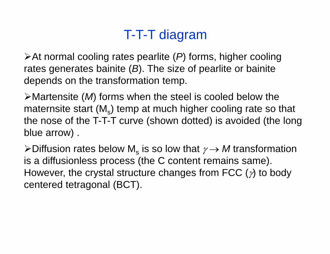
T-T-T diagramAt normal cooling rates pearlite (P) forms, higher cooling rates generates bainite (B). The size of pearlite or bainite depends on the transformation temp. Martensite (M) forms when the steel is cooled below the maternsite start (Ms) temp at much higher cooling rate so that the nose of the T-T-T curve (shown dotted) is avoided (the long blue arrow) .Diffusion rates below Ms is so low that M transformation is a diffusionless process (the C content remains same). However, the crystal structure changes from FCC () to body centered tetragonal (BCT).

C-C-T diagramIn actual practice a steel is generally cooled continuously. Continuous-cooling-transformation (C-C-T) diagrams depict this situation. The C-C-T curve (Blue) is shifted to the right of the T-T-T (dashed) curve as continuous cooling transformation occurs at lower temperature and longer time compared isothermal holding.

C-C-T diagramBainite generally does not form in steels during continuous cooling and hence the C-C-T curve ceases just below the nose.The microstructure (fine or coarse) depends on the cooling rate. Higher the cooling rate finer the microstructure is.Finer size pearlite is called sorbite and very fine size pearlite is called troostite.The critical cooling rate is the one at which the cooling curve just touches the nose of the C-C-T curve.A cooling rate higher than the critical rate is needed to form martensite.

ExamplesEx.1. A eutectoid steel is slowly cooled from 750 C to a temperature just below 727 C . Calculate the percentage of ferrite and cementite.Solution: Eutectoid composition – 0.8% C, Ferrite composition - 0.025% C and cementite – 6.67% C.Apply the lever rule to get the percentages as% Ferrite = 100* (6.67 – 0.80)/(6.67 – 0.025) = 88.3%%Cementite = 100* (0.80 – 0.025)/(6.67 – 0.025) = 11.7%

Ex.2. A carbon steel cooled from austenitic region contains 9.1% ferrite. What is the C content in the steel?

Let c be C content. Apply the lever rule0.091 = (6.67 – c)/(6.67 – 0.025) c = 0.1% C

References

http://www.ce.berkeley.edu/~paulmont/CE60New/heat_treatment.pdfhttp://www.ce.berkeley.edu/~paulmont/CE60New/transformation.pdfhttp://www.synl.ac.cn/org/non/zu1/knowledge/phase.pdfhttp://www.youtube.com/watch?v=3xP1U_oDnfU

Key words. Phase transformation; Nucleation; Homogeneous and heterogeneous nucleation; Growth; Fe-C phase diagram; Eutectoid reaction; T-T-T diagram; C-C-T diagram

Quiz1. What are the different stages of phase transformation?2. What are homogeneous and heterogeneous nucleation?3. Derive the expression for critical radius of the nucleus?4. What are the different phases present in the Fe-C system?5. How many invariants reactions are present in the Fe-C

system and what are those?6. What are microstructure of eutectoid, hypoeutectoid and

hypereuctectoid steels obtained under equilibrium conditions?

7. What are T-T-T and C-C-T diagrams? What is the fundamental difference between them?

8. What should be the conditions for forming martensite in steels?

9. Why is the martensitic transformation in steels a diffusionless process?

Quiz10. What are sorbite and troostite?11. A plain-carbon steel contains 93 wt% ferrite and 7 % Fe3C.

What is the average carbon content in the steel?12. A 0.9% C steel is slowly cooled from 900 C to a

temperature just below 727 C . Calculate the percentages of proeutectoid cementite and eutectoid ferrite?

13. A 0.4% C steel is slowly cooled from 940 C to (A) just above 727 C (B) just below 727 C.Calculate the amount of austenite and proeutectoid ferrite for case (A).Calculate the amount of proeutectoid ferrite and eutectoid ferrite and cementite for case (B).

CASE HARDENING

Introduction

Surface hardening is a process which includes a wide variety of techniques is used to improve the

wear resistance of parts without affecting the softer, tough interior of the part. This combination of

hard surface and resistance and breakage upon impact is useful in parts such as a cam or ring gear that

must have a very hard surface to resist wear, along with a tough interior to resist the impact that

occurs during operation. Further, the surface hardening of steels has an advantage over through

hardening because less expensive low-carbon and medium-carbon steels can be surface hardened

without the problems of distortion and cracking associated with the through hardening of thick

sections.

Casehardening

Casehardening produces a hard wear resistant surface or case over a strong, tough core.

Casehardening is ideal for parts which require a wear resistant surface and at the same time, must be

tough enough internally to withstand the applied loads. The steels best suited to casehardening are the

low carbon and low alloy steels. If high carbon steel is casehardened, the hardness penetrates the core

and causes brittleness. In casehardening, the surface of the metal is changed chemically by

introducing a high carbide or nitride content. The core is chemically unaffected.

When heat treated, the surface responds to hardening while the core toughens. The common forms of

casehardening are carburizing, cyaniding and nitriding.

The surface hardening by diffusion involves the chemical modification of a surface. The basic process

used is thermo-chemical because some heat is needed to enhance the diffusion of hardening species

into the surface and subsurface regions of part. The depth of diffusion exhibits time-temperature

dependence such that:

Case depth ≈ K √Time

where the diffusivity constant, K, depends on temperature, the chemical composition of the steel, and

the concentration gradient of a given hardening species. In terms of temperature, the diffusivity

constant increases exponentially as a function of absolute temperature. Concentration gradients

depend on the surface kinetics and reactions of a particular process.

Methods of hardening by diffusion include several variations of hardening species (such as carbon,

nitrogen, or boron) and of the process method used to handle and transport the hardening species to

the surface of the part. Process methods for exposure involve the handling of hardening species in

forms such as gas, liquid, or ions. These process variations naturally produce differences in typical

case depth and hardness (Table 1). Factors influencing the suitability of a particular diffusion method

include the type of steel (Table 3). It is also important to distinguish between total case depth and

effective case depth. The effective case depth is typically about two-thirds to three-fourths the total

case depth. The required effective depth must be specified so that the heat treatment can process the

parts for the correct time

at the proper temperature.

Carburizing

Carburizing is a casehardening process in which carbon is added to the surface of low carbon steel.

Thus, carburized steel has a high carbon surface and a low carbon interior. When the carburized steel

is heat treated, the case is hardened while the core remains soft and tough.

Carburizing is the addition of carbon to the surface of low-carbon steels at temperatures generally

between 850 and 950°C (1560 and 1740°F), at which austenite, with its high solubility for carbon, is

the stable crystal structure. Hardening is accomplished when the high-carbon surface layer is

quenched to form martensite so that a high-carbon martensitic case with good wear and fatigue

resistance is superimposed on a tough, low-carbon steel core.

Case hardness of carburized steels is primarily a function of carbon content. When the carbon content

of the steel exceeds about 0.50% additional carbon has no effect on hardness but does enhance

hardenability. Carbon in excess of 0.50% may not be dissolved, which would thus require

temperatures high enough to ensure carbon-austenite solid solution.

Case depth of carburized steel is a function of carburizing time and the available carbon potential at

the surface. The variation of case depth with carburizing time is shown in Figure-2.28. When

prolonged carburizing times are used for deep case depths, a high carbon potential produces a high

surface-carbon content, which may thus result in excessive retained austenite or free carbides. These

two micro structural elements both have adverse effects on the distribution of residual stress in the

case-hardened part. Consequently, a high carbon potential may be suitable for short carburizing times

but not for prolonged carburizing.

Carburizing steels for case hardening usually have base-carbon contents of about 0.2%, with the

carbon content of the carburized layer generally being controlled at between 0.8 and 1% C. However,

surface carbon is often limited to 0.9% because too high a carbon content can result in retained

austenite and brittle martensite.

Most steels that are carburized are killed steels (deoxidized by the addition of aluminum), which

maintain fine grain sizes to temperatures of about 1040°C. Steels made to coarse grain practices can

be carburized if a double quench provides grain refinement. Double quenching usually consists of a

direct quench and then a re-quench from a lower temperature.

In another method of carburizing, called "gas carburizing," some material rich in carbon is introduced

into the furnace atmosphere. The carburizing atmosphere is produced by the use of various gases or

by the burning of oil, wood, or other materials. When the steel parts are heated in this atmosphere,

carbon monoxide combines with the gamma iron to produce practically the same results as those

described under the pack carburizing process.

A third method of carburizing is that of "liquid carburizing." In this method the steel is placed in a

molten salt bath that contains the chemicals required to produce a case comparable with one resulting

from pack or gas carburizing.

Alloy steels with low carbon content as well as low carbon steels may be carburized by either of the

three processes. However, some alloys, such as nickel, tend to retard the absorption of carbon. As a

result, the time required to produce a given thickness of case varies with the composition of the metal.

Quenching:

All of the carburizing processes (pack, gas, liquid) require quenching from the carburizing

temperature or a lower temperature or reheating and quenching. Parts are then tempered to the desired

hardness.

Figure 2.28 Case depth vs. Carburizing time

Pack Carburizing

In this process, the part that is to be carburized is packed in a steel container so that it is completely

surrounded by granules of charcoal. The charcoal is treated with an activating chemical such as

Barium Carbonate (BaBO3) that promotes the formation of Carbon Dioxide (CO2). This gas in turn

reacts with the excess carbon in the charcoal to produce carbon monoxide; CO. Carbon Monoxide

reacts with the low-carbon steel surface to form atomic carbon which diffuses into the steel. Carbon

Monoxide supplies the carbon gradient that is necessary for diffusion. The carburizing process does

not harden the steel. It only increases the carbon content to some predetermined depth below the

surface to a sufficient level to allow subsequent quench hardening.

Carbon Monoxide reaction: CO2 + C ---> 2 CO

Reaction of Cementite to Carbon Monoxide: 2 CO + 3 Fe --->Fe3C + CO2

Figure 2.29 Pack carburizing process

Quenching Process:

It is difficult to quench the part immediately, as the sealed pack has to be opened and the part must be

removed from the pack. One technique that is used often is to slow cool the entire pack and

subsequently harden and temper the part after it is removed from the sealed pack.

Depth of Hardening:

There is no technical limit to the depth of hardening with carburizing techniques, but it is not common

to carburize to depths in excess of 0.050 in.

Carburizing Time: 4 to 10 hour

Gas Carburizing

Can be done with any carbonaceous gas, such as methane, ethane, propane, or natural gas. Most

carburizing gases are flammable and controls are needed to keep carburizing gas at 1700 oF from

contacting air (oxygen). The advantage of this process over pack carburizing is an improved ability to

quench from the carburizing temperature. Conveyor hearth furnaces make quenching in a controlled

atmosphere possible.

In gas carburizing, the parts are surrounded by a carbon-bearing atmosphere that can be continuously

replenished so that a high carbon potential can be maintained. While the rate of carburizing is

substantially increased in the gaseous atmosphere, the method requires the use of a multicomponent

atmosphere whose composition must be very closely controlled to avoid deleterious side effects, for

example, surface and grain-boundary oxides. In addition, a separate piece of equipment is required to

generate the atmosphere and control its composition. Despite this increased complexity, gas

carburizing has become the most effective and widely used method for carburizing steel parts in large

quantities.

In efforts required to simplify the atmosphere, carburizing in an oxygen-free environment at very low

pressure (vacuum carburizing) has been explored and developed into a viable and important

alternative. Although the furnace enclosure in some respects becomes more complex, the atmosphere

is greatly simplified. A single-component atmosphere consisting solely of a simple gaseous

hydrocarbon, for example methane, may be used. Furthermore, because the parts are heated in an

oxygen-free environment, the carburizing temperature may be increased substantially without the risk

of surface or grain-boundary oxidation. The higher temperature permitted increases not only the solid

solubility of carbon in the austenite but also its rate of diffusion, so that the time required to achieve

the case depth desired is reduced.

Although vacuum carburizing overcomes some of the complexities of gas carburizing, it introduces a

serious new problem that must be addressed. Because vacuum carburizing is conducted at very low

pressures, and the rate of flow of the carburizing gas into the furnace is very low, the carbon potential

of the gas in deep recesses and blind holes is quickly depleted. Unless this gas is replenished, a great

nonuniformity in case depth over the surface of the part is likely to occur. If, in an effort to overcome

this problem, the gas pressure is increased significantly, another problem arises, that of free-carbon

formation, or sooting.

Advantages of Gas Carburizing

It takes less time when compared with pack Carburizing method

Control is more accurate to achieve surface carbon content and case hardness

When compare with pack Carburizing, complicated shape components are carburised by this

method

Liquid Carburizing

Can be performed in internally or externally heated molten salt pots. Carburizing salt contains cyanide

compounds such as sodium cyanide (NaCN). Cycle times for liquid cyaniding is much shorter (1 to 4

hours) than gas and pack carburizing processes. Disadvantage is the disposal of salt. (Environmental

problems) and cost (safe disposal is very expensive).

In this process, the steel components are immersed in a liquefied carbon-rich bath of molten salts. The molten salt contains a mixture of sodium carbonate, sodium chloride and silicon carbide. The reaction in the bath is

This saturates the metal with carbon. The bath is replenished from time to time. The components are

immersed in the bath at a temperature of around 870 to 900oC. So that the carbon is diffused into the

surface of the steel. In this method the time required for carburising the metal surface of 0.2 to 0.3mm

in 35 to 55min. Then the metal is then undergone rapid quenching to lock the carbon inside the

structure. By this method uniform case hardening is obtained when compared with other methods.

Advantages of Liquid Carburizing

Uniform case hardening depth is obtained

Components are free from oxidation

Soot is not formed on the surface of the component

CASE HARDENING

Lecture 2 (continue)

Nitriding

Nitriding is unlike other casehardening processes in that, before nitriding, the part is heat treated to

produce definite physical properties. Thus, parts are hardened and tempered before being nitrided.

Most steels can be nitrided, but special alloys are required for best results. These special alloys

contain aluminum as one of the alloying elements and are called "nitralloys."

Principal reasons for nitriding are:

To obtain high surface hardness

To increase wear resistance and antigalling properties

To improve fatigue life

To improve corrosion resistance

To obtain a surface that is resistant to the softening effect of heat at temperatures up to the nitriding

temperature.

In nitriding, the part is placed in a special nitriding furnace and heated to a temperature of

approximately 1,000°F. With the part at this temperature, ammonia gas is circulated within the

specially constructed furnace chamber. The high temperature cracks the ammonia gas into nitrogen

and hydrogen. The ammonia which does not break down is caught in a water trap below the regions of

the other two gases. The nitrogen reacts with the iron to form nitride. The iron nitride is dispersed in

minute particles at the surface and works inward. The depth of penetration depends on the length of

the treatment. In nitriding, soaking periods as long as 72 hours are frequently required to produce the

desired thickness of case. Nitriding can be accomplished with a minimum of distortion, because of the

low temperature at which parts are casehardened and because no quenching is required after exposure

to the ammonia gas.

In this process, nitrogen is diffused into the surface of the steel being treated. The reaction of nitrogen

with the steel causes the formation of very hard iron and alloy nitrogen compounds. The resulting

nitride case is harder than tool steels or carburized steels. The advantage of this process is that

hardness is achieved without the oil, water or air quench. As an added advantage, hardening is

accomplished in a nitrogen atmosphere that prevents scaling and discoloration. Nitriding temperature

is below the lower critical temperature of the steel and it is set between 925 oF and 1050

oF. The

nitrogen source is usually Ammonia (NH3). At the nitriding temperature the ammonia dissociates into

Nitrogen and Hydrogen.

2NH3 ---> 2N + 3H

Figure 2.30 Nitriding process

The nitrogen diffuses into the steel and hydrogen is exhausted. A typical nitriding setup is illustrated

in Figure 2.30.

Figure 2.31

The white layer shown in Figure 4 has a detrimental effect on the fatigue life of nitrided parts, and it is

normally removed from parts subjected to severe service. Two stage gas-nitriding processes can be

used to prevent the formation of white layer. White layer thickness may vary between 0.0003 and

0.002 in. which depends on nitriding time. The most commonly nitrided steels are chromium-

molybdenum alloy steels and Nitralloys. Surface hardness of 55 HRC to 70 HRC can be achieved

with case depths varying from 0.005 in to 0.020 in. Nitrided steels are very hard and grinding

operations should not be performed after nitriding. White layer is removed by lapping.

Figure 2.31 Nitriding time for various types of alloy steels

CARBURISING Vs. NITRIDING

Gas nitriding is emerging as the significant surface hardening process for today's and future industry,

constituting a viable alternative to the well-established carburizing process. Most gears, shafts, hubs,

pins and other parts are carburized in mass production to various case depths with accurate carbon

potential control. Yet, carburizing is handicapped by several disadvantages. Below table compares

certain important features of the two processes.

Carbonitriding:

Carbonitriding is a modified form of gas carburizing, rather than a form of nitriding. The modification

consists of introducing ammonia into the gas carburizing atmosphere to add nitrogen to the carburized

case as it is being produced. Nascent nitrogen forms at the work surface by the dissociation of

ammonia in the furnace atmosphere; the nitrogen diffuses into the steel simultaneously with carbon.

Typically, carbonitriding is carried out at a lower temperature and for a shorter time than is gas

carburizing, producing a shallower case than is usual in production carburizing.

Carbonitriding is used primarily to impart a hard, wear-resistant case, generally from 0.075 to 0.75

mm (0.003 to 0.030 in.) deep. A carbonitrided case has better hardenability than a carburized case.

Consequently, by carbonitriding and quenching, a hardened case can be produced at less expense

within the case-depth range indicated, using either carbon or low-alloy steel. Full hardness with less

distortion can be achieved with oil quenching, or, in some instances, even gas quenching, employing a

protective atmosphere as the quenching medium.

Steels commonly carbonitrided include those in the AISI 1000, 1100, 1200, 1300, 1500, 4000, 4100,

4600, 5100, 6100, 8600, and 8700 series, with carbon contents up to about 0.25%. Also, many steels

in these same series with a carbon range of 0.30 to 0.50% are carbonitrided to case depths up to about

0.3 mm (0.01 in.) when a combination of a reasonably tough, through-hardened core and a hard, long-

wearing surface is required (shafts and transmission gears are typical examples). Steels such as 4140,

5130, 5140, 8640, and 4340 for applications like heavy-duty gearing are treated by this method at

845°C (1550°F).

Often, carburizing and carbonitriding are used together to achieve much deeper case depths and better

engineering performance for parts than could be obtained using only the carbonitriding process. This

process is applicable particularly with steels with low case hardenability, that is, the 1000, 1100, and

1200 series steels. The process generally consists of carburizing at 900 to 955°C (1650 to 1750°F) to

give the desired total case depth (up to 2.5 mm. or 0.100 in.), followed by carbonitriding for 2 to 6 h

in the temperature range of 815 to 900°C (1500 to 1650°F) to add the desired carbonitrided case

depth. The subject parts can then be oil quenched to obtain a deeper effective and thus harder case

than would have resulted from the carburizing process alone. The addition of the carbonitrided surface

increases the case residual compressive stress level and thus improves contact fatigue resistance as

well as increasing the case strength gradient.

When the carburizing/carbonitriding processes are used together, the effective case depth (50 HRC) to

total case depth ratio may vary from about 0.35 to 0.75 depending on the case hardenability, core

hardenability, section size, and quenchant used.

The fundamental problem in controlling carbonitriding processes is that the rate of nitrogen pick-up

depends on the free ammonia content of the furnace atmosphere and not the percentage of ammonia in

the inlet gas. Unfortunately, no state-of-the-art sensor for monitoring the free ammonia content of the

furnace atmosphere has yet been developed.

Case Composition. The composition of a carbonitrided case depends on the type of steel and on the

process variables of temperature, time, and atmosphere composition. In terms of steel type, the case

depth achieved during a given carbonitriding process will be lower in steels containing higher

amounts of strong nitride formers such as aluminum or titanium.

In terms of process variables, the higher the carbonitriding temperature, the less effective is the

ammonia addition to the atmosphere as a nitrogen source, because the rate of spontaneous

decomposition of ammonia to molecular nitrogen and hydrogen increases as the temperature is raised.

At a given temperature, the fraction of the ammonia addition that spontaneously decomposes is

dependent on the residence time of the atmosphere in the furnace: the higher the total flow of

atmosphere gases, the lower the fraction of the ammonia addition that decomposes to nitrogen and

hydrogen. The addition of ammonia to a carburizing atmosphere has the effect of dilution by the

following reaction:

2NH3 →N2 + 3H2

Dilution with nitrogen and hydrogen affects measurements of oxygen potential in a similar manner;

the carbon potential possible with given oxygen potential is higher in a carburizing atmosphere than in

a carbonitriding atmosphere. Water vapor content, however, is much less affected by this dilution.

Thus, the amount of dilution and its resulting effect on the atmosphere composition depends on the

processing temperature, the amount of ammonia introduced, and the ratio of the total atmosphere gas

flow rate to the volume of the furnace.

Depth of Case. Preferred case depth is governed by service application and by core hardness. Case

depths of 0.025 to 0.075 mm (0.001 to 0.003 in.) are commonly applied to thin pans that require wear

resistance under light loads. Case depths up to 0.75 mm (0.030 in.) may be applied to parts for

resisting high compressive loads. Case depths of 0.63 to 0.75 mm (0.025 to 0.030 in.) may be applied

to shafts and gears that are subjected to high tensile or compressive stresses caused by torsion,

bending, or contact loads.

Medium-carbon steels with core hardness of 40 to 45 HRC normally require less case depth than

steels with core hardness of 20 HRC or below. Low-alloy steels with medium-carbon content, such as

those used in automotive transmission gears, are often assigned minimum case depths of 0.2 mm

(0.008 in.).

Measurements of the case depths of carbonitrided parts may refer to effective case depth or total case

depth, as with reporting case depths for carburized parts. For very thin cases, usually only the total

case depth is specified. In general, it is easy to distinguish case and core microstructures in a

carbonitrided piece, particularly when the case is thin and is produced at a low carbonitriding

temperature; more difficulty is encountered in distinguishing case and core when high temperatures,

deep cases, and medium-carbon or high-carbon steels are involved. Whether or not the core has a

martensitic structure is also a contributing factor in case-depth measurements.

Hardenability of Case. One major advantage of carbonitnding is that the nitrogen absorbed during

processing lowers the critical cooling rate of the steel. That is, the hardenability of the case is

significantly greater when nitrogen is added by carbonitriding than when the same steel is only

carburized. This permits the use of steels on which uniform case hardness ordinarily could not be

obtained if they were only carburized and quenched. Where core properties are not important,

carbonitriding permits the use of low-carbon steels, which cost less and may have better machinability

or formability.

This process involves with the diffusion of both carbon and nitrogen into the steel surface. The

process is performed in a gas atmosphere furnace using a carburizing gas such as propane or methane

mixed with several percent (by volume) of ammonia. Methane or propane serve as the source of

carbon, the ammonia serves as the source of nitrogen. Quenching is done in a gas which is not as

severe as water quench. As a result of les severe quench, there is less distortion on the material to be

treated. A typical carbonitriding system is shown in the following slide. Case hardnesses of HRC 60

to 65 are achieved at the surface.( Not as high as nitrided surfaces.) Case depths of 0.003 to 0.030 in

can be accomplished by carbonitriding. One of the advantages of this process is that it can be applied

to plain carbon steels which give significant case depths. Carbonitriding gives less distortion than

carburizing. Carbonitriding is performed at temperatures above the transformation temperature of the

steels (1400 oF -to 1600

oF)

Figure 2.32

Applications. Although carbonitnding is a modified carburizing process, its applications are more

restricted than those of carburizing. As has been stated previously, carbonitriding is largely limited to

case depths of about 0.75 mm (0.03 in.) or less, while no such limitation applies to carburizing. Two

reasons for this are: carbonitriding is generally done at temperatures of 870°C (1600°F) and below,

whereas, because of the time factor involved, deeper cases are produced by processing at higher

temperatures; and the nitrogen addition is less readily controlled than is the carbon addition, a

condition that can lead to an excess of nitrogen, and, consequently, to high levels of retained austenite

and case porosity when processing times are too long.

The resistance of a carbonitrided surface to softening during tempering is markedly superior to that of

a carburized surface. Other notable differences exist in terms of residual-stress pattern, metallurgical

structure, fatigue and impact strength at for many applications, carbonitriding the less expensive steels

will provide properties equivalent to those obtained in gas carburized alloy steels.

1

ME 212 LABORATORY EXPERIMENT #3

HARDNESS TESTING AND AGE HARDENING

1. OBJECTIVE:

Our primary aim is to measure the Rockwell Hardness values for different materials and

estimate ultimate tensile strengths by the aid of conversion tables. We will also focus on

age hardening, the info on which can be found in the last part of this experiment sheet.

2. HARDNESS TESTING THEORY:

Hardness is usually defined as the resistance of a material to plastic penetration of its

surface. There are three main types of tests used to determine hardness:

• Scratch tests are the simplest form of hardness tests. In this test, various materials

are rated on their ability to scratch one another. Mohs hardness test is of this type.

This test is used mainly in mineralogy.

• In Dynamic Hardness tests, an object of standard mass and dimensions is bounced

back from a surface after falling by its own weight. The height of the rebound is

indicated. Shore hardness is measured by this method.

• Static Indentation tests are based on the relation of indentation of the specimen by

a penetrator under a given load. The relationship of total test force to the area or

depth of indentation provides a measure of hardness. The Rockwell, Brinell,

Knoop, Vickers, and ultrasonic hardness tests are of this type.

For engineering purposes, only the static indentation tests are used.

BRINELL HARDNESS TEST:

This test consists of applying a constant load, usually between 500 and 3000 kgf for a

specified time (10 to 30 s) using a 5- or 10-mm diameter hardened steel or tungsten

carbide ball on the flat surface of a workpiece.

2

Figure 1. Brinell Hardness Test Schematic

Hardness is determined by taking the mean diameter of the indentation and calculating

the Brinell hardness number (BHM or HB) by dividing the applied load by the surface

area of the indentation according to following formula :

( ) 2 2

2

PHB

D D D dπ=

− −

where P is load in kg; D ball diameter in mm; and d is the diameter of the indentation in

mm.

Calculations have already been made and are available in tabular form for various

combinations of diameters of impressions and load.

The Brinell hardness number followed by the symbol HB without any suffix numbers

denotes standard test conditions using a ball of 10 mm diameter and a load of 3,000 kg

applied for 10 to 15 s. For other conditions, the hardness number and symbol HB are

supplemented by numbers indicating the test conditions in the following order: diameter

of ball, load, and duration of loading.

For example, 75 HB 10/500/30 indicates a Brinell hardness of 75 measured with a ball of

10 mm diameter and a load of 500 kg applied for 30s.

3

However, the BHN is not a satisfactory physical concept since the above equation does

not give the mean pressure over the surface of the indentation. Meyer suggested that a

more rational definition of hardness than that proposed by Brinell, would be one based on

the projected area of the impression rather than the surface area. The mean pressure

between surface of the indenter and the indentation is equal to the load divided by the

projected area of the indentation. Meyer proposed that this mean pressure should be taken

as the measure of hardness. It is referred to as the Meyer hardness.

2

4Meyer Hardness

P

dπ=

VICKERS HARDNESS TEST:

The Vickers hardness test uses a square base diamond pyramid as the indenter. The

included angle between the opposite faces of the pyramid is l36°. The Vickers hardness

tester operates on the same basic principle as the Brinell tester, the numbers being

expressed in the terms of load and area of the impression. As a result of the indenter’s

shape, the impression on the surface of the specimen will be a square. The length of the

diagonal of the square is measured through a microscope fitted with an ocular micrometer

that contains movable knife-edges. The Vickers hardness values are calculated by the

formula:

( )( )22

2 sin2

1.8544P

PHVdd

α

= =

where P is the applied load in kg, and d is the diagonal length in mm.

Microhardness Test:

This term, unfortunately, is misleading, as it could refer to the testing of small hardness

values when it actually means the use of small indentations. Test loads are between 1 and

1,000 g. Two types of indenters are used for Microhardness testing: the 136° square-base

Vickers diamond pyramid described previously, and the elongated Knoop diamond

indenter.

4

Figure 2. Vickers Hardness Testing Schematic

ROCKWELL HARDNESS TEST:

This hardness test uses a direct reading instrument based on the principle of differential

depth measurement. Rockwell testing differs from Brinell testing in that the Rockwell

hardness number is based on an inverse relationship to the measurement of the additional

depth to which an indenter is forced by a heavy (major) load beyond the depth resulting

from a previously applied (minor) load. Initially a minor load is applied, and a zero

datum position is established. The major load is then applied for a specified period and

removed, leaving the minor load applied. The resulting Rockwell number represents the

difference in depth from zero datum position as a result of the application of major load.

The entire procedure requires only 5 to 10 s.

Use of a minor load greatly increases the accuracy of this type of test, because it

eliminates the effects of backlash in the measuring system and causes the indenter to

break through slight surface roughness.

The 1200 sphero-conical diamond indenter is used mainly for testing hard materials such

as hardened steels and cemented carbides. Hardened steel ball indenters with diameters

1/16, 1/8, 1/4, 1/2 in. are used for testing softer materials such as fully annealed steels,

softer grades of cast irons, and a wide variety of nonferrous metals.

In Rockwell testing, the minor load is 10 kgf, and the major load is 60, 100 or 150 kgf. In

superficial Rockwell testing, the minor load is 3 kgf, and major loads are 15, 30 or 45

kgf. In both tests, the indenter may be either a diamond cone or steel ball, depending

principally on the characteristics of the material being tested.

5

1. Depth of indentation under preliminary load (10 kg)

2. Increase in depth of indentation under additional load (140 kg)

3. Permanent increase of depth of indentation under preliminary load after removal of additional load, the

increase being expressed in units of 0002 mm

4. Rockwell hardness HRC = 100—e

Figure 3. Rockwell Hardness Tesing Schematic

There are 30 different Rockwell scales, defined by the combination of the indenter and

minor and major loads. The majority of applications are covered by the Rockwell C and

B scales for testing steel, brass, and other materials.

6

TEST LOCATION:

If indentation is placed too close to the edge of specimen, the workpiece edge will bulge,

and the hardness number will decrease accordingly. To ensure an accurate test, the

distance from the center of the indentation to the edge of the specimen must be at least

two and one-half diameters.

An indentation hardness test cold works the surrounding material. If another indentation

is placed within this cold worked area, the reading usually will be higher than the real

value. Generally, the softer the material, the more critical the spacing of indentations

becomes. However, a distance three diameters from the center of one indentation to

another is sufficient for most materials.

HARDNESS TESTING IN ESTIMATING OTHER MATERIAL PROPERTIES:

Hardness testing has always appeared attractive as a means of estimating other

mechanical properties of metals. There is an empirical relation between those properties

for most steels as follows:

0.35*UTS BHN= (in kg/mm2)

This equation is used to predict tensile strength of steels by means of hardness

measurement. A reasonable prediction of ultimate tensile strength may also be obtained

using the relation:

( )( )

( )

( )2

12.5 21 2

3 1 2

n

nVHNUTS n

n

−

− = − −

− −

where VHN is the Vickers Hardness number and n is the Meyer’s index.

The 0.2 percent offset yield strength can be determined with good precision from Vickers

hardness number according to the relation: (Hint: For steels, the yield strength can

generally be taken as 80% of the UTS as an approximation)

( )( )2

0.2 0.13

nVHNYS

−=

7

3. AGE HARDENING

Many Aluminum based alloys, certain steels, nickel-based superalloys and titanium

alloys are strengthened by a heat treatment process known as age hardening. The first

step in the precipitation hardening process is to solution treat the alloy to a temperature

T1 where only the primary phase α exists and then hold the sample at that temperature

until all the θ (secondary) phase dissolves in the primary phase, as in Fig. 4 seen below.

The alloy is then rapidly cooled (quenched) to a low temperature. The precipitation of the

θ -phase is thus prevented because the speed of formation of θ - phase particles cannot

reach the speed of the rapid cooling. The aging process which follows shortly thereafter

can either be applied at room temperature or at an elevated temperature T2 which is still

in the two-phase region. During aging, the intermediate phase “trapped” in the primary α

phase continously transforms into small precipitates of the secondary θ -phase through

diffusion mechanisms. The precipitate clusters formed in this way tend to strengthen the

material.

Figure 4. Age Hardening Process (image from www.farmingdale.edu)

In the early stages of aging, a large number of very small clusters of the secondary θ -

phase are formed. As the composition reaches its saturated normal state, the material

reaches its maximum hardness. The precipitates, however, continue to grow. The fine

precipitates disappear. They have grown larger, and as a result the tensile strength of the

material decreases. This is called overaging which can be seen in Fig. 5.

It must be noted that the age hardening process can only be applied on materials which

exhibit decreasing solubility with decreasing temperature.

8

Figure 5. Hardness and Tensile Strength with increasing time in age-hardened alloys

(image from www.farmingdale.edu)

4. TASKS :

1. Find Hardness Conversion Tables from the American Society for Mechanical

Engineers (ASME) Handbooks located in the References Section of the Library.

Convert following HRC's to HB and HV values using the tables : 40, 57, 62

2. Using the above converted values, calculate the UTS and YS values using the

empirical formulas given in the laboratory sheets. See the hint that is given prior

to the formula for YS0.2 .

3. Discuss the advantages and disadvantages of the Brinell, Vickers and Rockwell

Hardness Tests.

4. Which Rockwell scale would you use for testing aluminum alloys?

5. How would you measure the hardness of

a) unmovable part of a large machine which is very heavy to transport

b) an unknown alloy?

9

REFERENCES:

• ASM Metals’ Handbook

• Mechanical Testing of Materials, A. J. Fenner, Philosophical Library Inc., 1965

• Pollack, H. W., Materials Science and Metallurgy, Reston Pub. Co., Reston:1981

• Van Vlack, L. H., Materials Science for Engineers, Addison Wesly Pub. Co.,

Mass:1970

• Standards:

Conversion : ASTM E 140: 1956

Brinnell : DIN 50351, ASTM E 10-73, BS 240: Parti: 1961, TS 189

Vickers: DIN 50133, ASTM E 92-72, BS 427: Part 1: 1961, TS 207

Rockwell: DIN50103, ASTM E l8-74, BS 4175: Part 1: 1967, TS 14O

HARDNESS TESTING

1. OBJECTIVE:

Our primary aim is to measure the Rockwell Hardness values for different materials and estimate ultimate tensile strengths by the aid of conversion tables.

2. HARDNESS TESTING THEORY:

Hardness is usually defined as the resistance of a material to plastic penetration of its surface. There are three main types of tests used to determine hardness:

Scratch tests are the simplest form of hardness tests. In this test, various materials are rated on their ability to scratch one another. Mohs hardness test is of this type. This test is used mainly in mineralogy.

In Dynamic Hardness tests, an object of standard mass and dimensions is bounced

back from a surface after falling by its own weight. The height of the rebound is indicated. Shore hardness is measured by this method.

Static Indentation tests are based on the relation of indentation of the specimen by

a penetrator under a given load. The relationship of total test force to the area or depth of indentation provides a measure of hardness. The Rockwell, Brinell, Knoop, Vickers, and ultrasonic hardness tests are of this type.

For engineering purposes, only the static indentation tests are used.

BRINELL HARDNESS TEST:

This test consists of applying a constant load, usually between 500 and 3000 kgf for a specified time (10 to 30 s) using a 5- or 10-mm diameter hardened steel or tungsten carbide ball on the flat surface of a workpiece.

1

Figure 1. Brinell Hardness Test Schematic

Hardness is determined by taking the mean diameter of the indentation and calculating the Brinell hardness number (BHM or HB) by dividing the applied load by the surface area of the indentation according to following formula :

HB P

π

D 2 2

2 D − D − d

where P is load in kg; D ball diameter in mm; and d is the diameter of the indentation in mm.

Calculations have already been made and are available in tabular form for various combinations of diameters of impressions and load.

The Brinell hardness number followed by the symbol HB without any suffix numbers denotes standard test conditions using a ball of 10 mm diameter and a load of 3,000 kg applied for 10 to 15 s. For other conditions, the hardness number and symbol HB are supplemented by numbers indicating the test conditions in the following order: diameter of ball, load, and duration of loading.

For example, 75 HB 10/500/30 indicates a Brinell hardness of 75 measured with a ball of 10 mm diameter and a load of 500 kg applied for 30s.

2

However, the BHN is not a satisfactory physical concept since the above equation does not give the mean pressure over the surface of the indentation. Meyer suggested that a more rational definition of hardness than that proposed by Brinell, would be one based on the projected area of the impression rather than the surface area. The mean pressure between surface of the indenter and the indentation is equal to the load divided by the projected area of the indentation. Meyer proposed that this mean pressure should be taken as the measure of hardness. It is referred to as the Meyer hardness.

Meyer Hardness

4P

π d 2

VICKERS HARDNESS TEST:

The Vickers hardness test uses a square base diamond pyramid as the indenter. The included angle between the opposite faces of the pyramid is l36°. The Vickers hardness tester operates on the same basic principle as the Brinell tester, the numbers being expressed in the terms of load and area of the impression. As a result of the indenter’s shape, the impression on the surface of the specimen will be a square. The length of the diagonal of the square is measured through a microscope fitted with an ocular micrometer that contains movable knife-edges. The Vickers hardness values are calculated by the formula:

HV

2 P sin α 2

1.8544 P

d 2

d 2

where P is the applied load in kg, and d is the diagonal length in mm.

Microhardness Test:

This term, unfortunately, is misleading, as it could refer to the testing of small hardness values when it actually means the use of small indentations. Test loads are between 1 and 1,000 g. Two types of indenters are used for Microhardness testing: the 136° square-base Vickers diamond pyramid described previously, and the elongated Knoop diamond indenter.

3

Figure 2. Vickers Hardness Testing Schematic

ROCKWELL HARDNESS TEST:

This hardness test uses a direct reading instrument based on the principle of differential depth measurement. Rockwell testing differs from Brinell testing in that the Rockwell hardness number is based on an inverse relationship to the measurement of the additional depth to which an indenter is forced by a heavy (major) load beyond the depth resulting from a previously applied (minor) load. Initially a minor load is applied, and a zero datum position is established. The major load is then applied for a specified period and removed, leaving the minor load applied. The resulting Rockwell number represents the difference in depth from zero datum position as a result of the application of major load. The entire procedure requires only 5 to 10 s.

Use of a minor load greatly increases the accuracy of this type of test, because it eliminates the effects of backlash in the measuring system and causes the indenter to break through slight surface roughness.

The 1200 sphero-conical diamond indenter is used mainly for testing hard materials such

as hardened steels and cemented carbides. Hardened steel ball indenters with diameters 1/16, 1/8, 1/4, 1/2 in. are used for testing softer materials such as fully annealed steels, softer grades of cast irons, and a wide variety of nonferrous metals.

In Rockwell testing, the minor load is 10 kgf, and the major load is 60, 100 or 150 kgf. In superficial Rockwell testing, the minor load is 3 kgf, and major loads are 15, 30 or 45 kgf. In both tests, the indenter may be either a diamond cone or steel ball, depending principally on the characteristics of the material being tested.

4

1. Depth of indentation under preliminary load (10 kg)

2. Increase in depth of indentation under additional load (140 kg)

3. Permanent increase of depth of indentation under preliminary load after removal of additional load, the increase being expressed in units of 0002 mm

4. Rockwell hardness HRC = 100—e

Figure 3. Rockwell Hardness Tesing Schematic

There are 30 different Rockwell scales, defined by the combination of the indenter and minor and major loads. The majority of applications are covered by the Rockwell C and B scales for testing steel, brass, and other materials.

5

TEST LOCATION:

If indentation is placed too close to the edge of specimen, the workpiece edge will bulge, and the hardness number will decrease accordingly. To ensure an accurate test, the distance from the center of the indentation to the edge of the specimen must be at least two and one-half diameters.

An indentation hardness test cold works the surrounding material. If another indentation is placed within this cold worked area, the reading usually will be higher than the real value. Generally, the softer the material, the more critical the spacing of indentations becomes. However, a distance three diameters from the center of one indentation to another is sufficient for most materials.

HARDNESS TESTING IN ESTIMATING OTHER MATERIAL PROPERTIES:

Hardness testing has always appeared mechanical properties of metals. There is for most steels as follows:

attractive as a means of estimating other an empirical relation between those properties

UTS 0.35 * BHN (in kg/mm2)

This equation is used to predict tensile strength of steels by means of hardness measurement. A reasonable prediction of ultimate tensile strength may also be obtained using the relation:

n −2

UTS VHN 1 − n − 2 12.5 n − 2

3 1

− n − 2

where VHN is the Vickers Hardness number and n is the Meyer’s index.

The 0.2 percent offset yield strength can be determined with good precision from Vickers hardness number according to the relation: (Hint: For steels, the yield strength can generally be taken as 80% of the UTS as an approximation)

YS0.2

VHN 0.1 n− 2

3

6

Material Science

Prof. Satish V. Kailas Associate Professor

Dept. of Mechanical Engineering, Indian Institute of Science,

Bangalore – 560012 India

Chapter 6. Phase Diagrams

Many of the engineering materials possess mixtures of phases, e.g. steel, paints, and composites. The mixture of two or more phases may permit interaction between different phases, and results in properties usually are different from the properties of individual phases. Different components can be combined into a single material by means of solutions or mixtures. A solution (liquid or solid) is phase with more than one component; a mixture is a material with more than one phase. Solute does not change the structural pattern of the solvent, and the composition of any solution can be varied. In mixtures, there are different phases, each with its own atomic arrangement. It is possible to have a mixture of two different solutions!

A pure substance, under equilibrium conditions, may exist as either of a phase namely vapor, liquid or solid, depending upon the conditions of temperature and pressure. A phase can be defined as a homogeneous portion of a system that has uniform physical and chemical characteristics i.e. it is a physically distinct from other phases, chemically homogeneous and mechanically separable portion of a system. In other words, a phase is a structurally homogeneous portion of matter. When two phases are present in a system, it is not necessary that there be a difference in both physical and chemical properties; a disparity in one or the other set of properties is sufficient.

There is only one vapor phase no matter how many constituents make it up. For pure substance there is only one liquid phase, however there may be more than one solid phase because of differences in crystal structure. A liquid solution is also a single phase, even as a liquid mixture (e.g. oil and water) forms two phases as there is no mixing at the molecular level. In the solid state, different chemical compositions and/or crystal structures are possible so a solid may consist of several phases. For the same composition, different crystal structures represent different phases. A solid solution has atoms mixed at atomic level thus it represents a single phase. A single-phase system is termed as homogeneous, and systems composed of two or more phases are termed as mixtures or heterogeneous. Most of the alloy systems and composites are heterogeneous.

It is important to understand the existence of phases under various practical conditions which may dictate the microstructure of an alloy, thus the mechanical properties and

usefulness of it. Phase diagrams provide a convenient way of representing which state of aggregation (phase or phases) is stable for a particular set of conditions. In addition, phase diagrams provide valuable information about melting, casting, crystallization, and other phenomena.

Useful terminology:-

Component – is either pure metal and/or compounds of which an alloy is composed. The components of a system may be elements, ions or compounds. They refer to the independent chemical species that comprise the system.

System – it can either refer to a specific body of material under consideration or it may relate to the series of possible alloys consisting of the same components but without regard to alloy composition.

Solid solution – it consists of atoms of at least two different types where solute atoms occupy either substitutional or interstitial positions in the solvent lattice and the crystal structure of the solvent is maintained.

Solubility limit – for almost all alloy systems, at a specific temperature, a maximum of solute atoms can dissolve in solvent phase to form a solid solution. The limit is known as solubility limit. In general, solubility limit changes with temperature. If solute available is more than the solubility limit that may lead to formation of different phase, either a solid solution or compound.

Phase equilibrium – it refers to the set of conditions where more than one phase may exist. It can be reflected by constancy with time in the phase characteristics of a system. In most metallurgical and materials systems, phase equilibrium involves just solid phases. However the state of equilibrium is never completely achieved because of very slow rate of approach of equilibrium in solid systems. This leads to non-equilibrium or meta-stable state, which may persist indefinitely and of course, has more practical significance than equilibrium phases. An equilibrium state of solid system can be reflected in terms of characteristics of the microstructure, phases present and their compositions, relative phase amounts and their spatial arrangement or distribution.

Variables of a system – these include two external variables namely temperature and pressure along with internal variable such as composition (C) and number of phases (P). Number of independent variables among these gives the degrees of freedom (F) or variance. All these are related for a chosen system as follows:

2+=+ CFP

which is known as Gibbs Phase rule. The degrees of freedom cannot be less than zero so that we have an upper limit to the number of phases that can exist in equilibrium for a given system. For practical purpose, in metallurgical and materials field, pressure can be considered as a constant, and thus the condensed phase rule is given as follows:

1+=+ CFP

7.1 Equilibrium Phase Diagrams, Particle strengthening by precipitation and precipitation reactions

7.1.1 Equilibrium Phase Diagrams

A diagram that depicts existence of different phases of a system under equilibrium is termed as phase diagram. It is also known as equilibrium or constitutional diagram. Equilibrium phase diagrams represent the relationships between temperature and the compositions and the quantities of phases at equilibrium. In general practice it is sufficient to consider only solid and liquid phases, thus pressure is assumed to be constant (1 atm.) in most applications. These diagrams do not indicate the dynamics when one phase transforms into another. However, it depicts information related to microstructure and phase structure of a particular system in a convenient and concise manner. Important information, useful for the scientists and engineers who are involved with materials development, selection, and application in product design, obtainable from a phase diagram can be summarized as follows:

- To show phases are present at different compositions and temperatures under slow cooling (equilibrium) conditions.

- To indicate equilibrium solid solubility of one element/compound in another. - To indicate temperature at which an alloy starts to solidify and the range of

solidification. - To indicate the temperature at which different phases start to melt. - Amount of each phase in a two-phase mixture can be obtained.

A phase diagram is actually a collection of solubility limit curves. The phase fields in equilibrium diagrams depend on the particular systems being depicted. Set of solubility curves that represents locus of temperatures above which all compositions are liquid are called liquidus, while solidus represents set of solubility curves that denotes the locus of temperatures below which all compositions are solid. Every phase diagram for two or more components must show a liquidus and a solidus, and an intervening freezing range, except for pure system, as melting of a phase occurs over a range of temperature. Whether the components are metals or nonmetals, there are certain locations on the phase diagram where the liquidus and solidus meet. For a pure component, a contact point lies at the edge of the diagram. The liquidus and solidus also meet at the other invariant positions on the diagram. Each invariant point represents an invariant reaction that can occur only under a particular set of conditions between particular phases, so is the name for it!

Phase diagrams are classified based on the number of components in the system. Single component systems have unary diagrams, two-component systems have binary diagrams, three-component systems are represented by ternary diagrams, and so on. When more than two components are present, phase diagrams become extremely complicated and difficult to represent. This chapter deals mostly with binary phase diagrams.

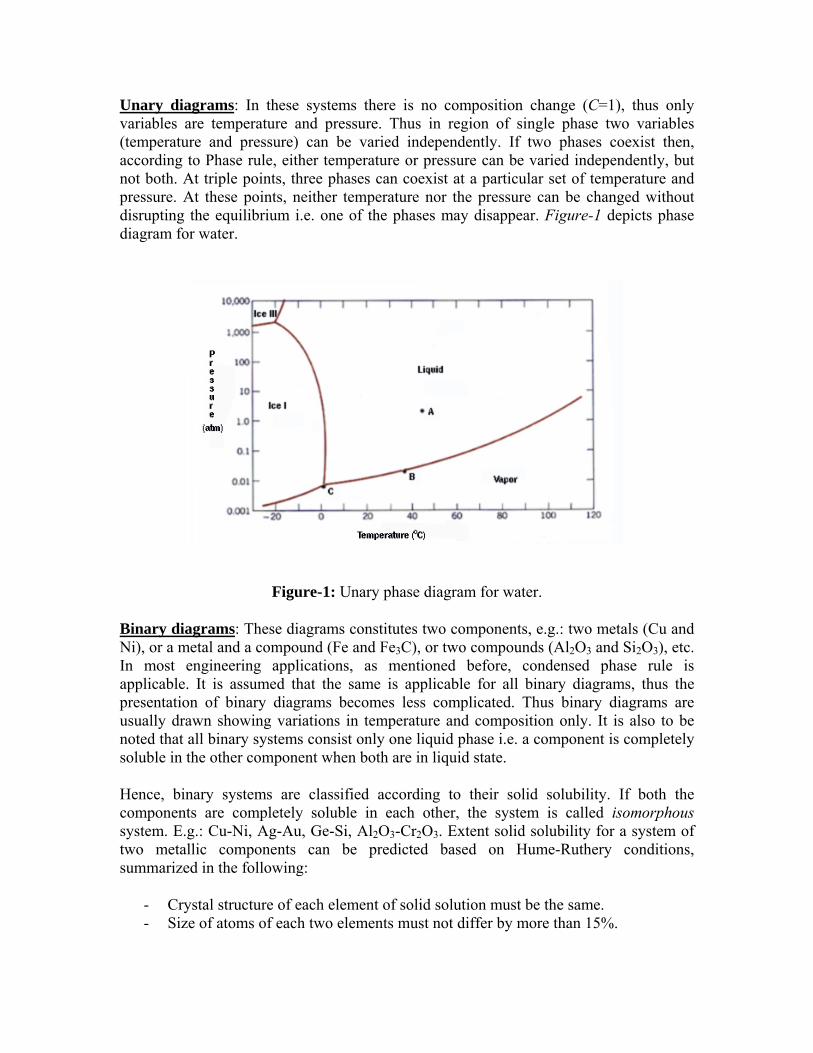
Unary diagrams: In these systems there is no composition change (C=1), thus only variables are temperature and pressure. Thus in region of single phase two variables (temperature and pressure) can be varied independently. If two phases coexist then, according to Phase rule, either temperature or pressure can be varied independently, but not both. At triple points, three phases can coexist at a particular set of temperature and pressure. At these points, neither temperature nor the pressure can be changed without disrupting the equilibrium i.e. one of the phases may disappear. Figure-1 depicts phase diagram for water.

Figure-1: Unary phase diagram for water.

Binary diagrams: These diagrams constitutes two components, e.g.: two metals (Cu and Ni), or a metal and a compound (Fe and Fe3C), or two compounds (Al2O3 and Si2O3), etc. In most engineering applications, as mentioned before, condensed phase rule is applicable. It is assumed that the same is applicable for all binary diagrams, thus the presentation of binary diagrams becomes less complicated. Thus binary diagrams are usually drawn showing variations in temperature and composition only. It is also to be noted that all binary systems consist only one liquid phase i.e. a component is completely soluble in the other component when both are in liquid state.

Hence, binary systems are classified according to their solid solubility. If both the components are completely soluble in each other, the system is called isomorphous system. E.g.: Cu-Ni, Ag-Au, Ge-Si, Al2O3-Cr2O3. Extent solid solubility for a system of two metallic components can be predicted based on Hume-Ruthery conditions, summarized in the following:

- Crystal structure of each element of solid solution must be the same. - Size of atoms of each two elements must not differ by more than 15%.

- Elements should not form compounds with each other i.e. there should be no appreciable difference in the electro-negativities of the two elements.

- Elements should have the same valence.

All the Hume-Rothery rules are not always applicable for all pairs of elements which show complete solid solubility.

In systems other than isomorphous systems i.e. in case of limited solid solubility, there exist solid state miscibility gaps; number of invariant reactions can take place; intermediate phases may exist over a range of composition (intermediate solid solutions) or only at relatively fixed composition (compound). These intermediate phases may undergo polymorphic transformations, and some may melt at a fixed temperature (congruent transformations, in which one phase changes to another of the same composition at definite temperature). A solid solution based on a pure component and extending to certain finite compositions into a binary phase diagram is called a terminal solid solution, and the line representing the solubility limit of a terminal solid solution w.r.t a two-phase solid region is called a solvus line (figure-4).

Isomorphous system: Figure-2 depicts a typical phase diagram for an isomorphous system made of two metallic elements A and B. As cited earlier, any phase diagram can be considered as a map. A set of coordinates – a temperature and a composition – is associated with each point in the diagram. If the alloy composition and temperature specified, then the phase diagram allows determination of the phase or phases that will present under equilibrium conditions. There are only two phases in the phase diagram, the liquid and the solid phases. These single-phases regions are separated by a two-phase region where both liquid and solid co-exist. The area in the figure-2 above the line marked liquidus (A’bB’) corresponds to the region of stability of the liquid phase, and the area below the solidus line (A’dB’) represents the stable region for the solid phase.

Figure-2: Phase diagram for typical isomorphous binary system.

For the interpretation of the phase diagram, let’s consider the vertical line ae drawn corresponding to composition of 50%A +50%B and assume that the system is undergoing equilibrium cooling. The point a on the line ae signifies that for that particular temperature and composition, only liquid phase is stable. This is true up to the point b which lies on the liquidus line, representing the starting of solidification. Completion of solidification of the alloy is represented by the point, d. Point e corresponds to single-phase solid region up to the room temperature. Point c lies in the two-phase region made of both liquid and solid phases. Corresponding micro-structural changes are also shown in figure-2. As shown in figure-2, above liquidus only a liquid phase exists, and below the solidus single solid phase exists as completely solidified grains. Between these two lines, system consist both solid crystals spread in liquid phase. It is customary to use L to represent liquid phase(s) and Greek alphabets (α, β, γ) for representing solid phases.

Between two extremes of the horizontal axis of the diagram, cooling curves for different alloys are shown in figure-3 as a function of time and temperature. Cooling curves shown in figure-3 represent A, U’, X, V’ and B correspondingly in figure-2. Change in slope of the cooling curve is caused by heat of fusion. In fact these changes in slope are nothing but points on either solidus or liquidus of a phase diagram. An experimental procedure where repeated cooling/heating of an alloy at different compositions, and corresponding changes in slope of cooling curves will be used to construct the phase diagram.

Figure-3: Cooling curves for isomorphous binary system.

Another important aspect of interpreting phase diagrams along with phases present is finding the relative amount of phases present and their individual composition.

Procedure to find equilibrium concentrations of phases:

- A tie-line or isotherm (UV) is drawn across two-phase region to intersect the boundaries of the region.

- Perpendiculars are dropped from these intersections to the composition axis, represented by U’ and V’ in figure-2, from which each of each phase is read. U’ represents composition of liquid phase and V’ represents composition of solid phase as intersection U meets liquidus line and V meets solidus line.

Procedure to find equilibrium relative amounts of phases (lever rule):

- A tie-line is constructed across the two phase region at the temperature of the alloy to intersect the region boundaries.

- The relative amount of a phase is computed by taking the length of tie line from overall composition to the phase boundary for the other phase, and dividing by the total tie-line length. From figure-2, relative amounts of liquid and solid phases is given respectively by

UVcVCL = ,

UVUcCS = , and it is to be noted that 1=+ SL CC .

Eutectic system: Many binary systems have components which have limited solid solubility, e.g.: Cu-Ag, Pb-Sn. The regions of limited solid solubility at each end of a phase diagram are called terminal solid solutions as they appear at ends of the diagram.

Many of the binary systems with limited solubility are of eutectic type, which consists of specific alloy composition known as eutectic composition that solidifies at a lower temperature than all other compositions. This low temperature which corresponds to the lowest temperature at which the liquid can exist when cooled under equilibrium conditions is known as eutectic temperature. The corresponding point on the phase diagram is called eutectic point. When the liquid of eutectic composition is cooled, at or below eutectic temperature this liquid transforms simultaneously into two solid phases (two terminal solid solutions, represented by α and β). This transformation is known as eutectic reaction and is written symbolically as:

Liquid (L) ↔ solid solution-1 (α) + solid solution-2 (β)

This eutectic reaction is called invariant reaction as it occurs under equilibrium conditions at a specific temperature and specific composition which can not be varied. Thus, this reaction is represented by a thermal horizontal arrest in the cooling curve of an alloy of eutectic composition. A typical eutectic type phase diagram is shown in figure-4 along with a cooling curve.

As shown in figure-4, there exist three single phase regions, namely liquid (L), α and β phases. There also exist three two phase regions: L+α, L+β and α+β. These three two phase regions are separated by horizontal line corresponding to the eutectic temperature. Below the eutectic temperature, the material is fully solid for all compositions. Compositions and relative amount of the phases can be determined using tie-lines and lever rule. Compositions that are on left-hand-side of the eutectic composition are known as hypo-eutectic compositions while compositions on right-hand-side of the eutectic composition are called hyper-eutectic compositions. Development of micro-structure and respective cooling curves for eutectic alloys are shown in figure-5, 6, 7 and 8 for different compositions. The phase that forms during cooling but before reaching eutectic temperature is called pro-eutectic phase.

Figure-4: Typical phase diagram for a binary eutectic system.

In many systems, solidification in the solid + liquid region may lead to formation of layered (cored) grains, even at very slow cooling rates. This is as a result of very slow or no-diffusion in solid state compared with very high diffusion rates in liquids. The composition of the liquid phase evolves by diffusion, following the equilibrium values that can be derived from the tie-line method. However, new layers that solidify on top of the grains have the equilibrium composition at that temperature but once they are solid their composition does not change.

Figure-5: Cooling curve and micro-structure development for eutectic alloy that passes mainly through terminal solid solution.

Figure-6: Cooling curve and micro-structure development for eutectic alloy that passes through terminal solid solution without formation of eutectic solid.

Figure-7: Cooling curve and micro-structure development for eutectic alloy that passes through hypo-eutectic region.

Figure-8: Cooling curve and micro-structure development for eutectic alloy that passes through eutectic-point.

Invariant reactions: The eutectic reaction, in which a liquid transforms into two solid phases, is just one of the possible three-phase invariant reactions that can occur in binary systems those are not isomorphous. Schematically it can be shown as in figure-9. It represents that a liquid phase, L, transforms into two different solids phases (α and β) upon cooling during the eutectic reaction.

Figure-9: Schematic of eutectic invariant reaction.

In the solid state analog of a eutectic reaction, called a eutectoid reaction, one solid phase having eutectoid composition transforms into two different solid phases. Another set of invariant reactions that occur often in binary systems are - peritectic reaction where a solid phase reacts with a liquid phase to produce a new solid phase, and in peritectoid reaction, two solid phases react to form a new solid phase. Peritectic reaction is commonly present as part of more-complicated binary diagrams, particularly if the melting points of the two components are quite different. Peritectic and peritectoid reactions do not give rise to micro-constituents as the eutectic and eutectoid reactions do. Another invariant reaction that involves liquid phase is monotectic reaction in which a liquid phase transforms into a solid phase and a liquid phase of different composition. Over a certain range of compositions the two liquids are immiscible like oil and water and so constitute individual phases, thus monotectic reaction can said to be associated with miscibility gaps in the liquid state. Example system for monotectic reaction: Cu-Pb at 954 C and 36%Pb. Analog to monotectic reaction in solid state is monotectoid reaction in which a solid phase transforms to produce two solid phases of different compositions. Another notable invariant reaction that is associated with liquid immiscibility is syntectic reaction in which two liquid phases react to form a solid phase. All the invariant reactions are summarized in the table-1 showing both symbolic reaction and schematic part of phase diagram.

Table-1: Summary of invariant reactions in binary systems.

Reaction Symbolic equation Schematic presentation Example

Eutectic L ↔ α + β

Fe-C, 4.27% C, 1147 C

Eutectoid α ↔ β + γ

Fe-C, 0.80% C, 723 C

Peritectic L + α ↔ β

Fe-C, 0.16%C, 1495 C

Peritectoid α + β ↔ γ

Monotectic L1 ↔ L2 + α

Fe-C, 0.51%C, 1495 C

Monotectoid α1 ↔ α2 + β

Syntectic L1 + L2 ↔ α

Intermediate phases: An intermediate phase may occur over a composition range (intermediate solid solution) or at a relatively fixed composition (compound) inside the phase diagram and are separated from other two phases in a binary diagram by two phase regions. Many phase diagrams contain intermediate phases whose occurrence cannot be readily predicted from the nature of the pure components. Intermediate solid solutions often have higher electrical resistivities and hardnesses than either of the two components. Intermediate compounds form relatively at a fixed composition when there exists a stoichiometric relationship between the components, for example: Mg2Ni and MgNi2 in Mg-Ni system. These are called inter-metallic compounds, and differ from other chemical compounds in that the bonding is primarily metallic rather than ionic or covalent, as would be found with compounds in certain metal-nonmetal or ceramic systems. Some metal-nonmetal compounds, Fe3C, are metallic in nature, whereas in others, MgO and Mg2Si, bonding is mainly covalent. When using the lever rules, inter-metallic compounds are treated like any other phase, except they appear not as a wide region but as a vertical line.

Number of phase transformations may takes place for each system. Phase transformations in which there are no compositional alternations are said to be congruent transformations, and during incongruent transformations at least one of the phases will experience a change in composition. Examples for (1) congruent transformations: allotropic transformations, and melting of pure materials (2) incongruent transformations: all invariant reactions, and also melting of alloy that belongs to an isomorphous system. Intermediate phases are sometimes classified on the basis of whether they melt congruently or incongruently. MgNi2, for example, melts congruently whereas Mg2Ni melts incongruently since it undergoes peritectic decomposition.

7.1.2 Particle strengthening by precipitation and precipitation reactions

As explained in an earlier chapter (chapter-6: Dislocations and Strengthening Mechanisms), by obstructing dislocation motion in different means, material’s strength can be increased. One of the methods that are applicable to multi-phase material is particle strengthening in which second phase particles are introduced into the matrix by either mixing-and-consolidation (dispersion strengthening) or precipitated in solid state (precipitation hardening).

The object of the precipitation strengthening is to create in a heat-treated alloy a dense and fine dispersion of precipitated particles in a matrix of deformable metal. The particles act as obstacles to dislocation motion. In order for an alloy system to be able to precipitation-strengthened for certain alloy compositions; there must be a terminal solid solution which has a decreasing solid solubility as the temperature decreases. For

example: Au-Cu in which maximum solid solubility of Cu in Al is 5.65% at 548 C that decreases with decreasing temperature.

The precipitation strengthening process involves the following three basic steps:

- Solutionizing (solution heat treatment), where the alloy is heated to a temperature between solvus and solidus temperatures and kept there till a uniform solid-solution structure is produced.

- Quenching, where the sample is rapidly cooled to a lower temperature (room temperature) and the cooling medium is usually water. Alloy structure in this stage consists of supersaturated solid solution.

- Aging is the last but critical step. During this heat treatment step finely dispersed precipitate particle will form. Aging the alloy at room temperature is called natural aging, whereas at elevated temperatures is called artificial aging. Most alloys require artificial aging, and aging temperature is usually between 15-25% of temperature difference between room temperature and solution heat treatment temperature.

Precipitation strengthening and reactions that occur during precipitation can be best illustrated using the Al-4%Cu (duralumin) system. Figure-10 depicts the Al-rich end of the Al-Cu phase diagram. It can be observed that the alloy with 4%Cu exists as a single phase α-solid solution at around 550 C, and at room temperature as a mixture of α (with less than 0.5%Cu) and an inter-metallic compound, CuAl2 (θ) with 52%Cu. On slow cooling α rejects excess Cu as precipitate particles of θ. These particles relatively coarse in size and can cause only moderate strengthening effect.

Figure-10: Aluminium rich end of Al-Cu phase diagram.

By rapidly cooling the alloy, a supersaturated solution can be obtained at room temperature. As a function of time at room temperature, and at higher temperatures up to 200 C, the diffusion of Cu atoms may take place and the precipitate particles can form. For this particular alloy, Al-4%Cu, five sequential structures can be identified: (a) supersaturated solid solution α, (b) GP1 zones, (c) GP2 zones (θ” phase), (d) θ’ phase and (e) θ phase, CuAl2. Not all these phases can be produced at all aging temperatures. GP1 and GP2 zones are produced at lower temperatures, and θ’ and θ phases occur at higher temperatures. The initial stages of precipitation are the most difficult to analyze because of the extremely small size of the particles and their relatively uniform distribution. GP zones meant for Guinier-Preston zones which have a definite composition and structure that is not the same as that of the final stable precipitate. Evidently these particles are easier to nucleate than the final precipitate, as a result, form first. Eventually they disappear as later more stable phases appear. θ” and θ’ are meta-stable transition precipitates with distinct crystal structure of their own, while θ is the equilibrium stable precipitate of CuAl2.

GP1 zones:- These zones are created by Cu atoms segregating in α, and the segregated regions are of disk shape with thickness of 0.4-0.6 nm, and 8-10 nm in diameter and form on the {100} cubic planes of the matrix. As Cu atoms which replace Al atoms are smaller in diameter, matrix lattice strains tetragonally. These zones are said to be coherent with the matrix lattice.

GP2 zones / θ” phase:- With additional aging, ordering of larger clumps of Cu atoms on {100} occurs. These zones have tetragonal structure which therefore introduces coherency in the lattice with {100} planes of the matrix, accompanied by further hardening. However, their size ranges from 1-4 nm thick and 10-100 nm in diameter as aging proceeds.

θ’ phase:- This phase nucleates heterogeneously especially on dislocations. It has tetragonal structure but is partially coherent with the matrix. This phase forms platelets with thickness 10-150 nm.

θ phase:- With still further aging the equilibrium phase CuAl2 or θ is formed from the transition lattice θ’ or directly from the matrix accompanied by a reduction in hardness. It has a BCT (body-centered-tetragonal) structure, and is incoherent with the matrix. As these particles are no longer coherent with the matrix, hardness is lower than at the stage when coherent was present. Over-aging continues with the growth of these particles controlled by diffusion. Variation of hardness with aging time is shown in figure-11.

The general sequence of precipitation in binary Al-Cu alloys can represented as:

Supersaturated α → GP1 zones → GP2 zones (θ” phase) → θ’ phase → θ phase (CuAl2)

Most precipitation-hardening systems operate in a similar way, peak hardness usually being attained in the later stages of coherency or at the onset of incoherency. It is quite common for a coherent precipitate to form and then lose coherency when the particle grows to a critical size. However, in some systems there is no evidence of coherency strains, and the fine particles appear to act alone as impediments to dislocation movements, for example – systems with dispersion strengthening.

Figure-11: Correlation of structures and hardness for Al-4%Cu alloy.

7.2 Kinetics of nucleation and growth

Structural changes in metallic systems usually take place by nucleation and growth whether it is just a phase change within one of the three states, or a simple structural rearrangement within a single phase, or a phase transformation. An equilibrium phase diagram presents the phases and phase changes expected under equilibrium conditions, but it provides no information about the rates of transformation. Although changes in pressure, composition, or temperature can cause phase transformations, it is temperature changes that are more important. From a micro structural standpoint, the first process to accompany a phase transformation is nucleation (i.e. the formation of very small particles or nuclei of the product phase from the parent phase) of the new phase particles which are capable of growing. The second stage is growth, in which the nucleated particles increase their size. The transformation reaches completion if growth of these new phase particles is allowed to proceed until the equilibrium fraction is attained.

Both nucleation and growth require that the accompanying free energy change be negative. Consequently, the super-heating or super-cooling that is necessary for a phase change is to be expected. That is a transformation cannot tale place precisely at the equilibrium transformation temperature because at that temperature free energies of phases are equal. In addition to temperature, two other factors that affect transformation rate – first, diffusion controlled rearrangement of atoms because of compositional and/or crystal structural differences; second, difficulty encountered in nucleating small particles via change in surface energy associated with the interface. Diffusion limits both the nucleation and growth rates in many cases.

With the nucleation of new particle, new interface is created between the particle and liquid. This interface will have positive energy that must be supplied during the transformation process. A tiny particle has a large surface area to volume ratio and therefore be unstable. Thus energy of the surface can effectively prevent the initial formation of a tiny particle. A particle said to have nucleated when it becomes stable and will not disappear due to thermal fluctuations. After a particle attained a critical size, it can grow further with a continuous decrease in energy. The surface energy is no longer a dominant factor in the growth process.

7.2.1 Nucleation kinetics

In homogeneous nucleation, the probability of nucleation occurring at any given site is identical to that at any other site within the volume of the parent phase. When a pure liquid metal is cooled below its equilibrium freezing temperature to a sufficient degree, numerous homogeneous nuclei are created by slow-moving atoms bonding together. Homogeneous nucleation usually requires a considerable amount of undercooling (cooling a material below the equilibrium temperature for a given transformation without the transformation occurring). Undercooling enhances the formation of nuclei that eventually grow. If ∆f is the free energy change accompanying the formation of a spherical new phase particle,

γππ 23 434 rgrf +Δ=Δ

where r is the radius of the particle, ∆g is the Gibbs free energy change per unit volume and γ is the surface energy of the interface. As surface energy, γ, is always positive, and ∆g is negative, passes through a maximum. From calculus, critical values can be found from the following:

gr

Δ−=

γ2* ; 23*hom )/(

316 gf Δ=Δ πγ

Particles which are smaller than the critical size are called embryos; those larger than the critical size are called nuclei. As ∆g becomes more negative with a lowering of the temperature, the critical values of ∆f and r becomes smaller as shown in figure-12. At sufficiently low temperatures, nucleation can be triggered by a few atoms statistically clustering as a nucleus, so a small critical radius is exceeded. With added growth, the new phase attains stability. Of course atom movements are sluggish at low temperatures, so growth is generally slow.

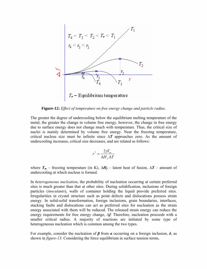
Figure-12: Effect of temperature on free energy change and particle radius.

The greater the degree of undercooling below the equilibrium melting temperature of the metal, the greater the change in volume free energy, however, the change in free energy due to surface energy does not change much with temperature. Thus, the critical size of nuclei is mainly determined by volume free energy. Near the freezing temperature, critical nucleus size must be infinite since ∆T approaches zero. As the amount of undercooling increases, critical size decreases, and are related as follows:

THT

rf

m

ΔΔ=

γ2*

where Tm – freezing temperature (in K), ∆Hf – latent heat of fusion, ∆T – amount of undercooling at which nucleus is formed.

In heterogeneous nucleation, the probability of nucleation occurring at certain preferred sites is much greater than that at other sites. During solidification, inclusions of foreign particles (inoculants), walls of container holding the liquid provide preferred sites. Irregularities in crystal structure such as point defects and dislocations possess strain energy. In solid-solid transformation, foreign inclusions, grain boundaries, interfaces, stacking faults and dislocations can act as preferred sites for nucleation as the strain energy associated with them will be reduced. The released strain energy can reduce the energy requirements for free energy change, ∆f. Therefore, nucleation proceeds with a smaller critical radius. A majority of reactions are initiated by some type of heterogeneous nucleation which is common among the two types.

For example, consider the nucleation of β from α occurring on a foreign inclusion, δ, as shown in figure-13. Considering the force equilibrium in surface tension terms,

βδαβαδ γθγγ += cos

where θ is the contact angle. An expression for ∆f can be written in terms of volume energy and surface energies as follows:

4coscos32)coscos32(

)(34 3

*hom

32

3* θθθθ

πγαβ +−Δ=+−

Δ=Δ f

gf het

Figure-13: Schematic of heterogeneous nucleation.

By comparing the free energy terms for homogeneous and heterogeneous nucleation processes for various contact conditions:

- When product particle makes only a point contact with the foreign surface, i.e. θ = 180 , the foreign particle does not play any role in the nucleation process →

*hom

* ff het Δ=Δ- If the product particle completely wets the foreign surface, i.e. θ = 0 , there is no

barrier for heterogeneous nucleation → 0* =Δ hetf- In intermediate conditions such as where the product particle attains

hemispherical shape, θ = 0 → *hom

*

21 ff het Δ=Δ

The above derivations are helpful in selecting a heterogeneous nucleation agent. It shows that a small contact angle is very helpful in heterogeneous nucleation. For a system of α –β interface, θ can be minimized by choosing δ such that energy of β- δ interface is kept to minimum. If the crystal structure two phases are similar and their lattice parameters are nearly equal, energy of the interface between those two phases will be minimum. This criterion is useful in selecting a agent for heterogeneous nucleation.

7.2.2 Growth kinetics

Many transformations occur as a result of continuous formation of critical nuclei in the parent phase and the subsequent growth of the particles. Growth is the increase in size of the particle after it has nucleated i.e. growth kinetics become important once an embryo has exceeded the critical size and become a stable nucleus. Growth may proceed in two

radically different manners. In one type of growth, individual atoms move independently from the parent to the product phase, thus it is diffusion controlled and is thermally activated. In the other type of growth that occurs in solid-solid transformations many atoms move cooperatively without thermal assistance. Growth that is diffusion controlled is more common the other.

Growth usually occurs by the thermally activated jump of atoms from the parent phase to the product phase. The unit step in the growth process thus consists of an atom leaving the parent phase and jumping across the interface to join the product phase. At the equilibrium temperature, both phases have the same free energy, hence the frequency of jumps from parent phase to product phase will be equal to that from product phase to parent phase i.e. the net growth rate is zero. At lower temperatures, product phase is expected to have lower free energy, and thus a net flow of atoms from parent phase to product phase. This net flux of atoms results in interface motion i.e. growth rate is taken as the rate of increase of a linear dimension of a growing particle. As a function of temperature, the growth rate first increases with increasing degree of supercooling, but eventually slows-down as thermal energy decreases. This is same as for nucleation; however the maximum in the growth rate usually occurs at a higher temperature than the maximum in the nucleation rate. Figure-14(a) depicts the temperature dependence of nucleation rate (U), growth rate (I) and overall transformation rate (dX/dt) that is a function of both nucleation rate and growth rate i.e. dX/dt= fn (U, I). On the other-hand, the time required for a transformation to completion has a reciprocal relationship to the overall transformation rate. Temperature dependence of this time is shown in figure-14 (b). The C-curve shown in figure-14(b) is characteristic of all thermally activated nucleation and growth transformations involving the transformation of a high-temperature phase to low-temperature phase. This curve is also known as time-temperature-transformation (TTT) curve. The nose of the C-curve corresponds to the minimum time for a specified fraction of transformation. It is also the place where overall transformation rate is a maximum.

(a) (b) Figure-14: (a) Temperature dependence of rates, (b) Time dependence of transformation

as a function of temperature.

In many investigations, the fraction of transformation that has occurred is measured as a function of time, while the temperature is maintained constant. Transformation progress

is usually ascertained by either microscopic examination or measurement of some physical property. Transformation data are plotted as the fraction of transformed material versus the logarithm of time, which results in characteristic S-curve (figure-15), largely because diffusion plays such an important role in both nucleation and growth. Conditions under which transformation may take place greatly affect the nature of the resulting microstructure. At small degrees of supercooling, where slow nucleation and rapid growth prevail, relatively coarse particles appear; at larger degrees of supercooling, relatively fine particles result. The time dependence of the transformation rate is an important consideration in the heat treatment of materials.

Figure-15: Fraction of transformation Vs the logarithm of time at constant temperature.

The other kind of growth involves congruent transformation which is considered as diffusion-less because it takes place at a rate approaching the speed of sound. It can be visualized as a cooperative type of process in which, without aid of thermal activation, atoms move into new locations because of the strain energy resulting from like movements of adjacent atoms. However the strains set-up in the parent phase may impede the further transformation, thus a lower temperature or mechanical deformation may be required to complete this martensitic transformation. The cooperative displacement of atoms here resembles a shear process during which, for example, FCC structure of Co transforms into HCP-Co or FCC-austenite into BCT-martensite. This merely requires that atoms in the FCC-phase move a fraction of an inter-atomic distance.

Because of its crystallographic nature, a martensitic transformation only occurs in the solid state. In addition, the crystal structure of the product phase must be easily generated from that of the parent phase without diffusive motion of atoms. This is true for most allotropic transformations in metals that occur at low temperatures or for high-temperature transformations of metals brought about by a quench. Reasons for martensitic transformation: (a) the free energy difference between the high-temperature phase and low-temperature phases becomes increasingly negative with decreasing temperature (b) the crystal structures of allotropes of a metal are relatively simple and share similar features with each other. It is also said that diffusion-controlled nucleation and growth and a martensitic change are competitive processes in many cases.

The martensitic transformation starts at a temperature designated Ms, which is generally below the equilibrium temperature, Te. The transformation is completed at a lower temperature, Mf. The amount of parent phase transformed into product phase depends on temperature only, and is independent of time. Furthermore, in most cases, Ms temperature and the fractional amount of product phase as a function of temperature are independent of quenching rate. Consequently, Ms and Mf are presented as horizontal lines on a TTT diagram. Catalytic effect of cold working can be used to make Ms approach Te. Martensitic transformations in Fe-C alloys and Ti are of great technological importance. Fe-C alloy transformations are dealt in detail in the following sections.

7.3 The iron – carbon system, phase transformations

A study of iron-carbon system is useful and important in many respects. This is because (1) steels constitute greatest amount of metallic materials used by man (2) solid state transformations that occur in steels are varied and interesting. These are similar to those occur in many other systems and helps explain the properties.

Iron-carbon phase diagram shown in figure-16 is not a complete diagram. Part of the diagram after 6.67 wt% C is ignored as it has little commercial significance. The 6.67%C represents the composition where an inter-metallic compound, cementite (Fe3C), with solubility limits forms. In addition, phase diagram is not true equilibrium diagram because cementite is not an equilibrium phase. However, in ordinary steels decomposition of cementite into graphite never observed because nucleation of cementite is much easier than that of graphite. Thus cementite can be treated as an equilibrium phase for practical purposes.

Figure-16: Iron – Iron carbide phase diagram.

The Fe-Fe3C is characterized by five individual phases and four invariant reactions. Five phases that exist in the diagram are: α–ferrite (BCC) Fe-C solid solution, γ-austenite (FCC) Fe-C solid solution, δ-ferrite (BCC) Fe-C solid solution, Fe3C (iron carbide) or cementite - an inter-metallic compound and liquid Fe-C solution. Four invariant reactions that cause transformations in the system are namely eutectoid, eutectic, monotectic and peritectic.

As depicted by left axes, pure iron upon heating exhibits two allotropic changes. One involves α–ferrite of BCC crystal structure transforming to FCC austenite, γ-iron, at 910

C. At 1400 C, austenite changes to BCC phase known as δ-ferrite, which finally melts at 1536 C.

Carbon present in solid iron as interstitial impurity, and forms solid solution with ferrites / austenite as depicted by three single fields represented by α, γ and δ. Carbon dissolves least in α–ferrite in which maximum amount of carbon soluble is 0.02% at 723 C. This limited solubility is attributed to shape and size of interstitial position in BCC α–ferrite. However, carbon present greatly influences the mechanical properties of α–ferrite. α–ferrite can be used as magnetic material below 768 C. Solubility of carbon in γ-iron reaches its maximum, 2.11%, at a temperature of 1147 C. Higher solubility of carbon in austenite is attributed to FCC structure and corresponding interstitial sites. Phase transformations involving austenite plays very significant role in heat treatment of different steels. Austenite itself is non-magnetic. Carbon solubility in δ-ferrite is maximum (0.1%) at 1495 C. As this ferrite exists only at elevated temperatures, it is of

no commercial importance. Cementite, Fe3C an inter-metallic compound forms when amount of carbon present exceeds its solubility limit at respective temperatures. Out of these four solid phases, cementite is hardest and brittle that is used in different forms to increase the strength of steels. α–ferrite, on the other hand, is softest and act as matrix of a composite material. By combining these two phases in a solution, a material’s properties can be varied over a large range.

For technological convenience, based on %C dissolved in it, a Fe-C solution is classified as: commercial pure irons with less than 0.008%C; steels having %C between 0.008-2.11; while cast irons have carbon in the range of 2.11%-6.67%. Thus commercial pure iron is composed of exclusively α–ferrite at room temperature. Most of the steels and cast irons contain both α–ferrite and cementite. However, commercial cast irons are not simple alloys of iron and carbon as they contain large quantities of other elements such as silicon, thus better consider them as ternary alloys. The presence of Si promotes the formation of graphite instead of cementite. Thus cast irons may contain carbon in form of both graphite and cementite, while steels will have carbon only in combined from as cementite.

As shown in figure-16, and mentioned earlier, Fe-C system constitutes four invariant reactions:

- peritectic reaction at 1495 C and 0.16%C, δ-ferrite + L ↔ γ-iron (austenite) - monotectic reaction 1495 C and 0.51%C, L ↔ L + γ-iron (austenite) - eutectic reaction at 1147 C and 4.3 %C, L ↔ γ-iron + Fe3C (cementite)

[ledeburite] - eutectoid reaction at 723 C and 0.8%C, γ-iron ↔ α–ferrite + Fe3C (cementite)

[pearlite]

Product phase of eutectic reaction is called ledeburite, while product from eutectoid reaction is called pearlite. During cooling to room temperature, ledeburite transforms into pearlite and cementite. At room temperature, thus after equilibrium cooling, Fe-C diagram consists of either α–ferrite, pearlite and/or cementite. Pearlite is actually not a single phase, but a micro-constituent having alternate thin layers of α–ferrite (~88%) and Fe3C, cementite (~12%). Steels with less than 0.8%C (mild steels up to 0.3%C, medium carbon steels with C between 0.3%-0.8% i.e. hypo-eutectoid Fe-C alloys) i.e. consists pro-eutectoid α–ferrite in addition to pearlite, while steels with carbon higher than 0.8% (high-carbon steels i.e. hyper-eutectoid Fe-C alloys) consists of pearlite and pro-eutectoid cementite. Phase transformations involving austenite i.e. processes those involve eutectoid reaction are of great importance in heat treatment of steels.

In practice, steels are almost always cooled from the austenitic region to room temperature. During the cooling upon crossing the boundary of the single phase γ-iron, first pro-eutectoid phase (either α–ferrite or cementite) forms up to eutectoid temperature. With further cooling below the eutectoid temperature, remaining austenite decomposes to eutectoid product called pearlite, mixture of thin layers of α–ferrite and cementite. Though pearlite is not a phase, nevertheless, a constituent because it has a definite

appearance under the microscope and can be clearly identified in a structure composed of several constituents. The decomposition of austenite to form pearlite occurs by nucleation and growth. Nucleation, usually, occurs heterogeneously and rarely homogeneously at grain boundaries. When it is not homogeneous, nucleation of pearlite occurs both at grain boundaries and in the grains of austenite. When austenite forms pearlite at a constant temperature, the spacing between adjacent lamellae of cementite is very nearly constant. For a given colony of pearlite, all cementite plates have a common orientation in space, and it is also true for the ferrite plates. Growth of pearlite colonies occurs not only by the nucleation of additional lamellae but also through an advance at the ends of the lamellae. Pearlite growth also involves the nucleation of new colonies at the interfaces between established colonies and the parent austenite. The thickness ratio of the ferrite and cementite layers in pearlite is approximately 8 to 1. However, the absolute layer thickness depends on the temperature at which the isothermal transformation is allowed to occur.

The temperature at which austenite is transformed has a strong effect on the inter-lamellar spacing of pearlite. The lower the reaction temperature, the smaller will be inter-lamellar spacing. For example, pearlite spacing is in order of 10-3 mm when it formed at 700 C, while spacing is in order of 10-4 mm when formed at 600 C. The spacing of the pearlite lamellae has a practical significance because the hardness of the resulting structure depends upon it; the smaller the spacing, the harder the metal. The growth rate of pearlite is also a strong function of temperature. At temperatures just below the eutectoid, the growth rate increases rapidly with decreasing temperature, reaching a maximum at 600 C, and then decreases again at lower temperatures.

Additions of alloying elements to Fe-C system bring changes (alternations to positions of phase boundaries and shapes of fields) depends on that particular element and its concentration. Almost all alloying elements causes the eutectoid concentration to decrease, and most of the alloying elements (e.g.: Ti, Mo, Si, W, Cr) causes the eutectoid temperature to increase while some other (e.g.: Ni, Mn) reduces the eutectoid temperature. Thus alloying additions alters the relative amount of pearlite and pro-eutectoid phase that form.

Fe-C alloys with more than 2.11% C are called cast irons. Phase transformations in cast irons involve formation of pro-eutectic phase on crossing the liquidus. During the further cooling, liquid of eutectic composition decomposes in to mixture of austenite and cementite, known as ledeburite. On further cooling through eutectoid temperature, austenite decomposes to pearlite. The room temperature microstructure of cast irons thus consists of pearlite and cementite. Because of presence of cementite, which is hard, brittle and white in color, product is called white cast iron. However, depending on cooling rate and other alloying elements, carbon in cast iron may be present as graphite or cementite. Gray cast iron contains graphite in form of flakes. These flakes are sharp and act as stress risers. Brittleness arising because of flake shape can be avoided by producing graphite in spherical nodules, as in malleable cast iron and SG (spheroidal graphite) cast iron. Malleable cast iron is produced by heat treating white cast iron (Si < 1%) for prolonged periods at about 900 C and then cooling it very slowly. The cementite decomposes and temper carbon appears approximately as spherical particles. SG iron is produced by

adding inoculants to molten iron. In these Si content must be about 2.5%, and no subsequent heat treatment is required.

7.4 Transformation rate effects and TTT diagrams, Microstructure and Property Changes in Fe-C Alloys

Solid state transformations, which are very important in steels, are known to be dependent on time at a particular temperature, as shown in figure-14(b). Isothermal transformation diagram, also known as TTT diagram, measures the rate of transformation at a constant temperature i.e. it shows time relationships for the phases during isothermal transformation. Information regarding the time to start the transformation and the time required to complete the transformation can be obtained from set of TTT diagrams. One such set of diagram for reaction of austenite to pearlite in steel is shown in figure-17. The diagram is not complete in the sense that the transformations of austenite that occur at temperatures below about 550 C are not shown.

Figure-17: Partial TTT diagram for a eutectoid Fe-C alloy.

As mentioned in previous section, thickness of layers in pearlite depends on the temperature at which the transformation occurred. If the transformation took place at a temperature that is just below the eutectoid temperature, relatively thick layers of α–ferrite and cementite are produced in what is called coarse pearlite. This is because of high diffusion rates of carbon atoms. Thus with decreasing transformation temperature, sluggish movement of carbon results in thinner layers α–ferrite and cementite i.e. fine pearlite is produced.

At transformation temperatures below 550 C, austenite results in different product known as bainite. Bainite also consists of α–ferrite and cementite phases i.e. transformation is again diffusion controlled but morphologically it consists of very small particles of cementite within or between fine ferrite plates. Bainite forms needles or plates, depending on the temperature of the transformation; the microstructural details of bainite are so fine that their resolution is only possible using electron microscope. It

differs from pearlite in the sense that different mechanism is involved in formation ob bainite which does not have alternating layers of α–ferrite and cementite. In addition, because of equal growth rates in all directions pearlite tends to form spherical colonies, whereas bainite grows as plates and has a characteristic acicular (needlelike) appearance. Upper bainite, formed at the upper end of the temperature range (550 C-350 C), is characterized by relatively coarse, irregular shaped cementite particles in α–ferrite plates. If the transformation is taking place at lower temperatures (350 C-250 C), the α–ferrite plates assume a more regular needlelike shape, and the transformation product is called lower bainite. At the same time carbide particles become smaller in size and appear as cross-striations making an angle of about 55 to the axis of the α–ferrite plate. Upper bainite has large rod-like cementite regions, whereas lower bainite has much finer cementite particles as a result of sluggish diffusion of carbon atoms at lower temperatures. Lower bainite is considerably harder than upper bainite. Another characteristic of bainite is that as it has crystallographic orientation that is similar to that found in simple ferrite nucleating from austenite, it is believed that bainite is nucleated by the formation of ferrite. This is in contrast to pearlite which is believed to be nucleated by formation of cementite.

Basically, bainite is a transformation product that is not as close to equilibrium as pearlite. The most puzzling feature of the bainite reaction is its dual nature. In a number of respects, it reveals properties that are typical of a nucleation and growth type of transformation such as occurs in the formation pearlite and also a mixture of α–ferrite and cementite though of quite different morphology (no alternate layers), but at the same time it differs from the Martensite as bainite formation is athermal and diffusion controlled though its microstructure is characterized by acicular (needlelike) appearance.

The time-temperature dependence of the bainite transformation can also be presented using TTT diagram. It occurs at temperatures below those at which pearlite forms i.e. it does not form until the transformation temperature falls below a definite temperature, designated as BBs. Above this temperature austenite does not form bainite except under external stresses. Below BsB , austenite does not transform completely to bainite. The amount of bainite formed increases as the isothermal reaction temperature is lowered. By reaching a lower limiting temperature, BBf, it is possible to transform austenite completely to bainite. The BsB and BBf temperatures are equivalent to the Ms and Mf temperatures for Martensite.

In simple eutectoid steels, pearlite and bainite transformations overlap, thus transition from the pearlite to bainite is smooth and continuous i.e. knees of individual pearlite and bainite curves are merged together. However each of the transformations has a characteristic C-curve, which can be distinguishable in presence of alloying elements. As shown in complete TTT diagram for eutectoid steel in figure-18, above approximately 550 C-600 C, austenite transforms completely to pearlite. Below this range up to 450

C, both pearlite and bainite are formed. Finally, between 450 C and 210 C, the reaction product is bainite only. Thus bainite transformation is favored at a high degree of supercooling, and the pearlite transformation at a low degree of supercooling. In middle region, pearlitic and bainitic transformations are competitive with each other.

Figure-18: Complete TTT (isothermal transformation) diagram for eutectoid steel.

As explained in earlier section, martensitic transformation can dominate the proceedings if steel is cooled rapid enough so that diffusion of carbon can be arrested. Transformation of austenite to Martensite is diffusion-less, time independent and the extent of transformation depends on the transformation temperature. Martensite is a meta-stable phase and decomposes into ferrite and pearlite but this is extremely slow (and not noticeable) at room temperature. Alloying additions retard the formation rate of pearlite and bainite, thus rendering the martensitic transformation more competitive. Start of the transformation is designated by Ms, while the completion is designated by Mf in a transformation diagram. Martensite forms in steels possesses a body centered tetragonal crystal structure with carbon atoms occupying one of the three interstitial sites available. This is the reason for characteristic structure of steel Martensite instead of general BCC. Tetragonal distortion caused by carbon atoms increases with increasing carbon content and so is the hardness of Martensite. Austenite is slightly denser than Martensite, and therefore, during the phase transformation upon quenching, there is a net volume increase. If relatively large pieces are rapidly quenched, they may crack as a result of internal stresses, especially when carbon content is more than about 0.5%.

Mechanically, Martensite is extremely hard, thus its applicability is limited by brittleness associated with it. Characteristics of steel Martensite render it unusable for structural applications in the as-quenched form. However, structure and thus the properties can be altered by tempering, heat treatment observed below eutectoid temperature to permit diffusion of carbon atoms for a reasonable period of time. During tempering, carbide particles attain spherical shape and are distributed in ferrite phase – structure called spheroidite. Spheroidite is the softest yet toughest structure that steel may have. At lower

tempering temperature, a structure called tempered Martensite forms with similar microstructure as that of spheroidite except that cementite particles are much, much smaller. The tempering heat treatment is also applicable to pearlitic and bainitic structures. This mainly results in improved machinability. The mechanism of tempering appears to be first the precipitation of fine particles of hexagonal ε-carbide of composition about Fe2.4C from Martensite, decreasing its tetragonality. At higher temperatures or with increasing tempering times, precipitation of cementite begins and is accompanied by dissolution of the unstable ε-carbide. Eventually the Martensite loses its tetragonality and becomes BCC ferrite, the cementite coalesces into spheres. A schematic of possible transformations involving austenite decomposition are shown in figure-19.

Figure-19: Possible transformation involving austenite decomposition.

Tempering of some steels may result in a reduction of toughness what is known as temper embrittlement. This may be avoided by (1) compositional control, and/or (2) tempering above 575 or below 375, followed by quenching to room temperature. The effect is greatest in Martensite structures, less severe in bainitic structures and least severe in pearlite structures. It appears to be associated with the segregation of solute atoms to the grain boundaries lowering the boundary strength. Impurities responsible for temper brittleness are: P, Sn, Sb and As. Si reduces the risk of embrittlement by carbide formation. Mo has a stabilizing effect on carbides and is also used to minimize the risk of temper brittleness in low alloy steels.

TTT diagrams are less of practical importance since an alloy has to be cooled rapidly and then kept at a temperature to allow for respective transformation to take place. However, most industrial heat treatments involve continuous cooling of a specimen to room temperature. Hence, Continuous Cooling Transformation (CCT) diagrams are generally more appropriate for engineering applications as components are cooled (air cooled, furnace cooled, quenched etc.) from a processing temperature as this is more economic than transferring to a separate furnace for an isothermal treatment. CCT diagrams measure the extent of transformation as a function of time for a continuously decreasing temperature. For continuous cooling, the time required for a reaction to begin and end is delayed, thus the isothermal curves are shifted to longer times and lower temperatures.

Both TTT and CCT diagrams are, in a sense, phase diagrams with added parameter in form of time. Each is experimentally determined for an alloy of specified composition. These diagrams allow prediction of the microstructure after some time period for constant temperature and continuous cooling heat treatments, respectively. Normally, bainite will not form during continuous cooling because all the austenite will have transformed to pearlite by the time the bainite transformation has become possible. Thus, as shown in figure-20, region representing austenite-pearlite transformation terminates just below the nose.

Figure-20: Superimposition of TTT and CCT diagrams for a eutectoid steel.

References

1. G. E. Dieter, Mechanical Metallurgy, Third Edition, McGraw-Hill, New York, 1986.

2. William D. Callister, Jr, Materials Science and Engineering – An introduction, sixth edition, John Wiley & Sons, Inc. 2004.

3. D. Hull, Introduction of Dislocations, Third Edition, Butterworth-Heinemann, Woburn, UK, 1984

1

1. GENERAL KNOWLEDGE

1.1. Basic principles of non-destructive testing (NDT)

1.1.1. Definition and importance of NDT

Non-destructive testing is the use of physical methods which will test materials, components and assemblies for flaws in their structure without damaging their future usefulness. NDT is concerned with revealing flaws in the structure of a product. It, however, cannot predict where flaws will develop due to the design itself.

All NDT methods have the following common characteristics:

(a) The application of a testing medium to the product to be tested.

(b) The changes in the testing medium due to the defects in the structure of the product.

(c) A means by which it detects these changes.

(d) Interpretation of these changes to obtain information about the flaws in the structure of the product.

Importance of NDT

NDT plays an important role in the quality control of a product. It is used during all the stages of manufacturing of a product. It is used to monitor the quality of the:

(a) Raw materials which are used in the construction of the product.

(b) Fabrication processes which are used to manufacture the product.

(c) Finished product before it is put into service.

Use of NDT during all stages of manufacturing results in the following benefits:

(a) It increases the safety and reliability of the product during operation.

(b) It decreases the cost of the product by reducing scrap and conserving materials, labour and energy.

(c) It enhances the reputation of the manufacturer as producer of quality goods.

All of the above factors boost the sales of the product which bring more economical benefits to the manufacturer.

NDT is also used widely for routine or periodic determination of quality of the plants and structures during service. This not only increases the safety of operation but also eliminates any forced shut down of the plants.

1.1.2. Types of NDT methods

The methods of NDT range from the simple to the complicated. Visual inspection is the simplest of all. Surface imperfections invisible to the eye may be revealed by penetrant or magnetic methods. If really serious surface defects are found, there is often little point in proceeding to more complicated examinations of the interior by ultrasonics or radiography. NDT methods may be divided into groups for the purposes of these notes: conventional and non-conventional. To the first group may belong the methods which are commonly used and include visual or optical inspection, dye penetrant testing, magnetic particle testing, eddy current testing,

2

radiographic testing and ultrasonic testing. The second group of NDT methods are those used only for specialized applications and consequently are limited in use. Some of these methods which are being mentioned here merely as a curiosity for the reader include neutron radiography, acoustic emission, thermal and infrared testing, strain sensing, microwave techniques, leak testing, holography etc. It must also be remembered that no one of these methods can give us solutions to all the possible problems, i.e. they are not optional alternatives but rather complementary to each other. The basic principles, typical applications, advantages and limitations of the methods of group one will now be briefly described.

1.1.3. Visual testing (VT)

Often overlooked in any listing of NDT methods, visual inspection is one of the most common and most powerful means of non-destructive testing. Visual testing requires adequate illumination of the test surface and proper eye-sight of the tester. To be most effective visual inspection does however, merit special attention because it requires training (knowledge of product and process, anticipated service conditions, acceptance criteria, record keeping, for example) and it has its own range of equipment and instrumentation. It is also a fact that all defects found by other NDT methods ultimately must be substantiated by visual inspection. Visual testing can be classified as direct visual testing, remote visual testing and translucent visual testing. The most common NDT methods MT and PT are indeed simply scientific ways of enhancing the indication to make it more visible. Often the equipment needed is simple Figure 1.1 a portable light, a mirror on stem, a 2× or 4× hand lens, one illuminated magnifier with magnification 5x or 10×. For internal inspection, light lens systems such as borescopes allow remote surfaces to be examined . More sophisticated devices of this nature using fibre optics permit the introduction of the device into very small access holes and channels. Most of these systems provide for the attachment of a camera to permit permanent recording.

Figure 1.1: Various optical aids used in visual inspection.

(a) Mirror on stem: may be flat for normal view or concave for limited magnification.

(b) Hand magnifying glass (magnification usually 2–3×).

(c) Illuminated magnifier; field of view more restricted than D (magnification 5–10×).

(d) Inspection glass, usually fitted with a scale for measurement; the front surface is placed in contact with the work (magnification 5–10×).

(e) Borescope or intrascope with built-in illumination (magnification 2–3×).

3

The applications of visual testing include:

(1) Checking of the surface condition of the test specimen.

(2) Checking of alignment of mating surfaces.

(3) Checking of shape of the component.

(4) Checking for evidence of leaking.

(5) Checking for internal side defects.

1.1.4. Liquid penetrant testing (PT)

This is a method which can be employed for the detection of open-to-surface discontinuities in any industrial product which is made from a non-porous material. This method is widely used for testing of non-magnetic materials. In this method a liquid penetrant is applied to the surface of the product for a certain predetermined time, after which the excess penetrant is removed from the surface. The surface is then dried and a developer is applied to it. The penetrant which remains in the discontinuity is absorbed by the developer to indicate the presence as well as the location, size and nature of the discontinuity. The process is illustrated in Figure 1.2.

Penetrants used are either visible dye penetrant or fluorescent dye penetrant. The inspection for the presence of visible dye indications is made under white light while inspection of presence of indications by fluorescent dye penetrant is made under ultraviolet (or black) light under darkened conditions. The liquid penetrant processes are further sub-divided according to the method of washing of the specimen. The penetrants can be: (i) water-washable, (ii) post-emulsifiable, i.e. an emulsifier is added to the excess penetrant on surface of the specimen to make it water-washable, and (iii) solvent removable, i.e. the excess penetrant is needed to be dissolved in a solvent to remove it from the test specimen surface. In order of decreasing sensitivity and decreasing cost, the liquid penetrant processes can be listed as:

(1) Post emulsifiable fluorescent dye penetrant.

(2) Solvent removable fluorescent dye penetrant.

(3) Water washable fluorescent dye penetrant.

(4) Post emulsifiable visible dye penetrant.

(5) Solvent removable visible dye penetrant.

(6) Water washable visible dye penetrant.

Some of the advantages of liquid penetrant testing are as follows:

(1) Relatively low cost.

(2) Highly portable NDT method.

(3) Highly sensitive to fine, tight discontinuities.

(4) Fairly simple method.

(5) Can be used on a variety of materials.

(6) All surface discontinuities are detected in one operation, regardless of orientation.

4

Figure 1.2: Different stages of liquid penetrant process.

5

Some of the limitations of liquid penetrant testing are as follows:

(1) Test surface must be free of all contaminants (dirt, oil, grease, paint, rust, etc.).

(2) Detects surface discontinuities only.

(3) Cannot be used on porous specimens and is difficult to use on very rough surfaces.

(4) Removal of all penetrant materials, following the test, is often required.

(5) There is no easy method to produce permanent record.

1.1.5. Magnetic particle testing (MT)

Magnetic particle testing is used for the testing of materials which can be easily magnetized. This method is capable of detecting open to surface and just below the surface flaws. In this method the test specimen is first magnetized either by using a permanent or an electromagnet or by passing electric current through or around the specimen. The magnetic field thus introduced into the specimen is composed of magnetic lines of force. Whenever there is a flaw which interrupts the flow of magnetic lines of force, some of these lines must exit and re-enter the specimen. These points of exit and re-entry form opposite magnetic poles. Whenever minute magnetic particles are sprinkled onto the surface of such a specimen, these particles are attracted by these magnetic poles to create a visual indication approximating the size and shape of the flaw. Figure 1.3 illustrates the basic principles of this method.

Figure 1.3: Basic principle of magnetic particle testing.

6

Depending on the application, there are different magnetization techniques used in magnetic particle testing. These techniques can be grouped into the following two categories:

(a) Direct current techniques: These are the techniques in which the current flows through the test specimen and the magnetic field produced by this flow of current is used for the detection of defects. These techniques are shown in Figure 1.4 (a, b & c).

(b) Magnetic flux flow techniques: In these techniques magnetic flux is induced into the specimen either by the use of a permanent magnet or by flowing current through a coil or a conductor. These techniques are shown in Figure 1.4 (d–g).

Figure 1.4: Different magnetizations used in magnetic particle testing.

7

Advantages of magnetic particle testing include the following:

(1) It does not need very stringent pre-cleaning operation.

(2) Best method for the detection of fine, shallow surface cracks in ferromagnetic material.

(3) Fast and relatively simple NDT method.

(4) Generally inexpensive.

(5) Will work through thin coating.

(6) Few limitations regarding the size/shape of test specimens.

(7) Highly portable NDT method.

(8) It is quicker.

Some of the limitations of magnetic particle testing include the following:

(1) Material must be ferromagnetic.

(2) Orientation and strength of magnetic field is critical.

(3) Detects surface and near-to-surface discontinuities only.

(4) Large currents sometimes required.

(5) “Burning” of test parts a possibility.

(6) Parts must often be demagnetized, which may be difficult.

1.1.6. Eddy current testing (ET)

This method is widely used to detect surface flaws, to sort materials, to measure thin walls from one surface only, to measure thin coatings and in some applications to measure case depth. This method is applicable to electrically conductive materials only. In the method eddy currents are produced in the product by bringing it close to an alternating current carrying coil. The alternating magnetic field of the coil is modified by the magnetic fields of the eddy currents. This modification, which depends on the condition of the part near to the coil, is then shown as a meter reading or cathode ray tube presentation. Figure 1.5 gives the basic principles of eddy current testing.

There are three types of probes Figure 1.6 used in eddy current testing. Internal probes are usually used for the in-service testing of heat exchanger tubes. Encircling probes are commonly used for the testing of rods and tubes during manufacturing. The uses of surface probes include the location of cracks, sorting of materials, measurement of wall and coating thickness, and case depth measurement.

This method may be used for:

(1) For the detection of defects in tubings.

(2) For sorting materials.

(3) For measurement of thin wall thickness’ from one surface only.

(4) For measuring thin coatings.

(5) For measuring case depth.

8

Figure 1.5: (a) Generation of eddy currents in the test specimen.

Figure 1.5: (b) Distortion of eddy currents due to defect.

Some of the advantages of eddy current testing include:

(1) Does not require couplant.

(2) It gives instantaneous response.

(3) Has uncomplicated steps during set-up.

(4) Is extremely sensitive to flaws.

(5) Is very repeatable.

(6) High scanning speeds can be used.

(7) Is very accurate for dimensional analysis of flaws or coating thickness.

9

(a) Internal Coil

(b) Encircling Coil

(c) Surface Probe

Figure 1.6: Types of probes used in eddy current testing.

Some of the limitations of eddy current testing include the following:

(1) The theory requires a good academic background in electrical principles and in mathematics.

(2) Extremely sensitive to surface variations and therefore requires a good surface.

(3) It is applicable to conductor materials only.

(4) Can be used on non-magnetic and magnetic material but is not reliable on carbon steel for the detection of subsurface flaws.

(5) Its depth of penetration is limited.

(6) Crack tightness and orientation of eddy current flow to a crack or linear discontinuity will affect detectability.


Unit 2

Alloys, substitutional and interstitial solid solutions- Phase diagrams: Interpretation of binary phase

diagrams

PHASE EQUILIBRIA AND PHASE DIAGRAMS

Phase diagrams are one of the most important sources of information concerning the behaviour of elements,

compounds and solutions. They provide us with the knowledge of phase composition and phase stability as a

function of temperature (T), pressure (P) and composition (C). Furthermore, they permit us to study and

control important processes such as phase separation, solidification, sintering, purification, growth and

doping of single crystals for technological and other applications. Although phase diagrams provide

information about systems at equilibrium, they can also assist in predicting phase relations, compositional

changes and structures in systems not at equilibrium

1. GASES, LIQUIDS AND SOLIDS

Any material (elemental or compound) can exist as a gas, a liquid or a solid, depending on the relative

magnitude of the attractive interatomic or intermolecular forces vs the disruptive thermal forces. It is thus

clear that the stability (existence) of the different states of aggregation, which are referred to as phases, is a

function of temperature and pressure (since with increased pressure the atoms, for example of a gas phase,

are closer spaced and thus subject to increased interatomic attraction).

In general terms, a “phase” is a homogeneous, physically distinct, mechanically separable portion of a

material with a given chemical composition. To illustrate this definition, let us look at a few examples of

common multi-phase systems. Ice cubes in water constitute a two-phase system (ice and liquid water),

unless we include the vapor above the glass in our system, which would make it a three-phase system. A

mixture of oil and water would also be a two-phase system. Just as oil and water represent two distinct

liquid phases, two regions of a solid with distinctly different composition or structure separated by

boundaries represent two solid phases.

If we look at a one-component system, such as liquid water, we recognize that because of the energy

distribution of the water molecules, some water molecules will always possess sufficient energy to overcome

the attractive forces on the surface of H2O and enter into the gas phase. If thermal energy is continuously

supplied to a liquid in an open container, the supply of high energy molecules (which leave the liquid phase)

is replenished and the temperature remains constant – otherwise the loss of high energy molecules will lower

the temperature of the system. The total quantity of heat necessary to completely “vaporize” one mole of a

liquid at its boiling point is called its molar heat of vaporization, designated by HV. Similarly, the heat

required to completely melt one mole of a solid (the heat required to break the bonds established in the solid

phase) is called the (latent) heat of fusion ( HV).

Visualize a liquid in a sealed container with some space above the liquid surface. Again, some of the most

energetic liquid molecules will leave the liquid phase and form a “gas phase” above the liquid. Since gas

molecules will thus accumulate in the gas phase (at a constant temperature), it is inevitable that as a result of

collisions in the gas phase some molecules will re-enter the liquid phase and a situation will be established

whereby the rate of evaporation will equal the rate of condensation – i.e., a dynamic equilibrium between

the liquid and gas phase will exist. The established pressure in the gas phase is referred to as the equilibrium

vapor pressure, which is normally significantly less for solids than for liquids.

For obvious reasons it is desirable to know for any given material the conditions (P, T) under which the

solid state, the liquid state and the gaseous state are stable, as well as the conditions under which the solid

and liquid phases may coexist. These conditions are graphically presented in equilibrium phase diagrams,

which can be experimentally determined.

2. THE ONE-COMPONENT PHASE DIAGRAM

Figure 1 illustrates the temperatures and pressures at which water can exist as a solid, liquid or vapor. The

curves represent the points at which two of the phases coexist in equilibrium. At the point Tt vapor, liquid

and solid coexist in equilibrium. In the fields of the diagram (phase fields) only one phase exists. Although

a diagram of this kind delineates the boundaries of the phase fields, it does not indicate the quantity of any

phase present.

It is of interest to consider the slope of the liquid/solid phase line of the H2O phase diagram. It can readily

be seen that if ice – say at –2°C – is subjected to high pressures, it will transform to liquid H2O. (An ice

skater will skate not on ice, but on water.) This particular pressure sensitivity (reflected in the slope of the

solid/liquid phase line) is characteristic for materials which have a higher coordination number in the

liquid than in the solid phase (H2O, Bi, Si, Ge). Metals, for example have an opposite slope of the

solid/liquid phase line, and the liquid phase will condense under pressure to a solid phase.

Fig. 1 Pressure/Temperature Diagram for Water.

3. PHASE RULE AND EQUILIBRIUM

The phase rule, also known as the Gibbs phase rule, relates the number of components and the number of

degrees of freedom in a system at equilibrium by the formula

F = C – P + 2 [1]

where F equals the number of degrees of freedom or the number of independent variables, C equals the

number of components in a system in equilibrium and P equals the number of phases. The digit 2 stands for

the two variables, temperature and pressure.

The number of degrees of freedom of a system is the number of variables that may be changed

independently without causing the appearance of a new phase or disappearance of an existing phase.

The number of chemical constituents that must be specified in order to describe the composition of each

phase present. For example, in the reaction involving the decomposition of calcium carbonate on heating,

there are three phases – two solid phases and one gaseous phase.

CaCO3 (s) � CaO (s) + CO2 (g) [2]

There are also three different chemical constituents, but the number of components is only two because any

two constituents completely define the system in equilibrium. Any third constituent may be determined if

the concentration of the other two is known. Substituting into the phase rule (eq. [1]) we can see that the

system is univariant, since F = C – P + 2 = 2 – 3 + 2 = 1. Therefore, only one variable, either temperature or

pressure, can be changed independently. (The number of components is not always easy to determine at first

glance, and it may require careful examination of the physical conditions of the system at equilibrium.)

The phase rule applies to dynamic and reversible processes where a system is heterogeneous and in

equilibrium and where the only external variables are temperature, pressure and concentration. For one-

component systems the maximum number of variables to be considered is two – pressure and

temperature. Such systems can easily be represented graphically by ordinary rectangular coordinates. For

two-component (or binary) systems the maximum number of variables is three – pressure, temperature

and concentration. Only one concentration is required to define the composition since the second

component is found by subtracting from unity. A graphical representation of such a system requires a

three-dimensional diagram. This, however, is not well suited to illustration and consequently separate

two-coordinate diagrams, such as pressure vs temperature, pressure vs composition and temperature vs

composition, are mostly used. Solid/liquid systems are usually investigated at constant pressure, and thus

only two variables need to be considered – the vapour pressure for such systems can be neglected. This is

called a condensed system and finds considerable application in studying phase equilibria in various

engineering materials. A condensed system will be represented by the following modified phase rule

equation:

F = C – P + 1 [3]

where all symbols are the same as before, but (because of a constant pressure) the digit 2 is replaced

by the digit 1, which stands for temperature as variable. The graphical representation of a solid/liquid

binary system can be simplified by representing it on ordinary rectangular coordinates: temperature

vs concentration or composition.

4. H vs T PHASE DIAGRAM

With the aid of a suitable calorimeter and energy reservoir, it is possible to measure the heat required to melt

and evaporate a pure substance like ice. The experimental data obtainable for a mole of ice is shown

schematically in fig. 2. As heat is added to the solid, the temperature rises along line “a” until the

temperature of fusion (Tf) is reached. The amount of heat absorbed per mole during melting is represented

by the length of line “b”, or HF. The amount of heat absorbed per mole during evaporation at the boiling

point is represented by line “d”. The reciprocal of the slope of line “a”, (dH/dT), is the heat required to

change the temperature of one mole of substance (at constant pressure) by 1°CF. (dH/dT) is the molar heat

capacity of a material, referred to as “C”. As the reciprocal of line “a” is C (solid), the reciprocals of lines

“c” and “e” are Cp (liquid) and Cp (vapour) respectively

Fig. 2 H vs T Diagram for Pure H2O.

From a thermodynamic standpoint, it is important to realize that fig. 2 illustrates the energy changes

that occur in the system during heating. Actual quantitative measurements show that 5.98 kJ of heat

are absorbed at the melting point (latent heat of fusion) and 40.5 kJ per mole (latent heat of

evaporation) at the boiling point. The latent heats of fusion and evaporation are unique characteristics

of all pure substances. Substances like Fe, Co, Ti and others, which are allotropic (exhibit different

structures at different temperatures), also exhibit latent heats of transformation as they change from

one solid state crystal modification to another.

5. ENERGY CHANGES

When heat is added from the surroundings to a material system (as described above), the energy of

the system changes. Likewise, if work is done on the surroundings by the material system, its energy

changes. The difference in energy ( E) that the system

experiences must be the difference between the heat absorbed (Q) by the system and the work (W)

done on the surroundings. The energy change may therefore be written as:

E = Q – W [4]

If heat is liberated by the system, the sign of Q is negative and work done is positive. Q and W

depend on the direction of change, but E does not. The above relation is one way of representing the

First Law of Thermodynamics which states that the energy of a system and its surroundings is

always conserved while a change in energy of the system takes place. The energy change, E, for a

process is independent of the path taken in going from the initial to the final state.

In the laboratory most reactions and phase changes are studied at constant pressure. The work is

then done solely by the pressure (P), acting through the volume change,

V.

W = P V and P = 0 [5]

Hence:

Q = E + P V [6]

Since the heat content of a system, or the enthalpy H, is defined by:

H = E + PV [7]

H = E + P V [8]

so that:

H = Q – W + P V [9]

or

H = Q [10]

Reactions in which H is negative are called exothermic since they liberate heat, whereas endothermic

reactions absorb heat. Fusion is an endothermic process, but the reverse reaction, crystallization, is an

exothermic one.

6. ENTROPY AND FREE ENERGY

When a gas condenses to form a liquid and a liquid freezes to form a crystalline solid, the degree of

internal order increases. Likewise, atomic vibrations decrease to zero when a perfect crystal is

cooled to 0°K. Since the term entropy, designated by S, is considered a measure of the degree of

disorder of a system, a perfect crystal at 0°K has zero entropy.

The product of the absolute temperature, T, and the change in entropy, S, is called the entropy factor,

T S. This product has the same units (Joules/mole) as the change in enthalpy, H, of a system. At

constant pressure, P, the two energy changes are related

to one another by the Gibbs free energy relation:

F = H – T S [11]

where

F = H – TS [12]

The natural tendency exhibited by all materials systems is to change from one of higher to one of

lower free energy. Materials systems also tend to assume a state of greater disorder whereby the

entropy factor T S is increased. The free energy change, F, expresses the balance between the two

opposing tendencies, the change in heat content (H) and the change in the entropy factor (T S).

If a system at constant pressure is in an equilibrium state, such as ice and water at 0°C, for example, at

atmospheric pressure it cannot reach a lower energy state. At

equilibrium in the ice-water system, the opposing tendencies, H and T S, equal one

another so that F = 0. At the fusion temperature, TF:

�S

F

�

�HF

[13]

TF

Similarly, at the boiling point:

�S

V

�

�HV

[14]

TV

Thus melting or evaporation only proceed if energy is supplied to the system from the

surroundings.

The entropy of a pure substance at constant pressure increases with temperature according to

the expression:

�S �

Cp�T

(since : �H � Cp�T) [15]

T

where Cp is the heat capacity at constant pressure, Cp, H, T and T are all

measurable quantities from which S and F can be calculated.

7. F vs T

Any system can change spontaneously if the accompanying free energy change is negative. This may

be shown graphically by making use of F vs T curves such as those shown in fig. 3.

Fig. 3 Free energy is a function of temperature for ice and water.

The general decrease in free energy of all the phases with increasing temperature is the result of

the increasing dominance of the temperature-entropy term. The increasingly negative slope for

phases which are stable at increasingly higher temperatures is the result of the greater entropy of

these phases.

PHASE DIAGRAMS (TWO-COMPONENT SYSTEMS)

1. SOLID SOLUTIONS

A solution can be defined as a homogeneous mixture in which the atoms or molecules of one

substance are dispersed at random into another substance. If this definition is applied to solids, we

have a solid solution. The term “solid solution” is used just as “liquid solution” is used because the

solute and solvent atoms (applying the term solvent to the element in excess) are arranged at

random. The properties and composition of a solid solution are, however, uniform as long as it is

not examined at the atomic or molecular level.

Solid solutions in alloy systems may be of two kinds: substitutional and interstitial. A substitutional

solid solution results when the solute atoms take up the positions of the solvent metal in the crystal

lattice. Solid solubility is governed by the comparative size of the atoms of the two elements, their

structure and the difference in electronegativity. If the atomic radii of a solvent and solute differ by

more than 15% of the radius of the solvent, the range of solubility is very small. When the atomic

radii of two elements are equal or differ by less than 15% in size and when they have the same

number of valency electrons, substitution of one kind of atom for another may occur with no

distortion or negligible distortion of the crystal lattice, resulting in a series of homogeneous solid

solutions. For an unlimited solubility in the solid state, the radii of the two elements must not differ

by more than 8% and both the solute and the solvent elements must have the same crystal structure.

In addition to the atomic size factor, the solid solution is also greatly affected by the electronegativity

of elements and by the relative valency factor. The greater the difference between electronegativities,

the greater is the tendency to form compounds and the smaller is the solid solubility. Regarding

valency effect, a metal of lower valency is more likely to dissolve a metal of higher valency.

Solubility usually increases with increasing temperature and decreases with decreasing temperature.

This causes precipitation within a homogeneous solid solution phase, resulting in hardening effect of

an alloy. When ionic solids are considered, the valency of ions is a very important factor.

2. CONSTRUCTION OF EQUILIBRIUM PHASE DIAGRAMS

OF TWO-COMPONENT SYSTEMS

To construct an equilibrium phase diagram of a binary system, it is a necessary and sufficient

condition that the boundaries of one-phase regions be known. In other words, the equilibrium diagram

is a plot of solubility relations between components of the system. It shows the number and

composition of phases present in any system under equilibrium conditions at any given temperature.

Construction of the diagram is often based on solubility limits determined by thermal analysis – i.e.,

using cooling curves. Changes in volume, electrical conductivity, crystal structure and dimensions

can also be used in constructing phase diagrams.

The solubility of two-component (or binary) systems can range from essential insolubility to

complete solubility in both liquid and solid states, as mentioned above. Water and oil, for

example, are substantially insoluble in each other while water and

alcohol are completely intersoluble. Let us visualize an experiment on the water-ether system in

which a series of mixtures of water and ether in various proportions is placed in test tubes. After

shaking the test tubes vigorously and allowing the mixtures to settle, we find present in them only

one phase of a few percent of ether in water or water in ether, whereas for fairly large percentages of

either one in the other there are two phases. These two phases separate into layers, the upper layer

being ether saturated with water and the lower layers being water saturated with ether. After

sufficiently increasing the temperature, we find, regardless of the proportions of ether and water, that

the two phases become one. If we plot solubility limit with temperature as ordinate and composition

as abscissa, we have an isobaric [constant pressure (atmospheric in this case)] phase diagram, as

shown in fig. 4. This system exhibits a solubility gap.

One phase

Two phases

Fig. 4 Schematic representation of the solubilities of ether and water in each other

Tem

per

ature

0 20 40 60 80 100

Composition percent, water

100 80 60 40 20 0

Composition percent, ether

3. COOLING CURVES

Fig. 5 Cooling curves: (a) pure compound; (b) binary solid solution; (c) binary

eutectic system.

SOLID SOLUTION EQUILIBRIUM DIAGRAMS

Fig. 6 Plotting equilibrium diagrams from cooling curves for Cu-Ni solid

solution alloys. (a) Cooling curves; (b) equilibrium diagram.

5. INTERPRETATION OF PHASE DIAGRAMS

From the above discussion we can draw two useful conclusions which are the only rules

necessary for interpreting equilibrium diagrams of binary systems.

Rule 1 - Phase composition: To determine the composition of phases which are stable at a given

temperature we draw a horizontal line at the given temperature. The projections (upon the abscissa) of

the intersections of the isothermal line with the liquidus and the solidus give the compositions of the

liquid and solid, respectively, which coexist in equilibrium at that temperature. For example, draw a

horizontal temperature line through temperature Te in fig. 7. The Te line intersects the solidus at f and

the liquidus at g, indicating solid composition of f% of B and (100–f)% of A. The liquid composition

at this temperature is g% of B and (100–g)% of A. This line in a two-phase region is known as a tie

line because it connects or “ties” together lines of one-fold saturation – i.e., the solid is saturated with

respect to B and the liquid is saturated with respect to A.

Rule 2 - The Lever Rule: To determine the relative amounts of the two phases, erect an ordinate at a

point on the composition scale which gives the total or overall composition of the alloy. The

intersection of this composition vertical and a given isothermal line is the fulcrum of a simple lever

system. The relative lengths of the lever arms multiplied by the amounts of the phase present must

balance. As an illustration, consider alloy � in fig. 7. The composition vertical is erected at alloy �

with a composition of e% of B and (100–e)% of A. This composition vertical intersects the

temperature horizontal (Te) at point e. The length of the line “f–e–g” indicates the total amount of the

two phases present. The length of line “e–g” indicates the amount of solid. In other words:

egfg x 100 � % of solid present

fgfg x 100 � % of liquid present

These two rules give both the composition and the relative quantity of each phase present in a two-

phase region in any binary system in equilibrium regardless of physical form of the two phases. The

two rules apply only to two-phase regions.

6. ISOMORPHOUS SYSTEMS

An isomorphous system is one in which there is complete intersolubility between the two

components in the vapor, liquid and solid phases, as shown in fig. 9. The Cu-Ni system is both a

classical and a practical example since the monels, which enjoy extensive commercial use, are

Cu-Ni alloys. Many practical materials systems are isomorphous.

Fig. 9 Schematic phase diagram for a binary system, A-B, showing complete

intersolubility (isomorphism) in all phases.

by mukesh kumar

assistant professor

darbhanga college of engineering

ENGINEERING material

2

Structures of Metals

Space lattices

Atom presents in any crystalline material are arranged in a regular three dimensional repeating pattern. this pattern is known as space lattice or crystal lattice.

Space lattices

The point of interaction of lines are called lattice point.

Unit cell

A unit cell is the smallest geometrical figure the repetition of which in three dimensions will give the actual crystal structure.

A unit cell is a building block of a crystal. the crystal consist of unit cell of stacked tightly together.

Each identical in shape, size and orientation with each other.

Unit cell

A unit cell is completely defined by

six lattice parameters.

a, b, c , a, b, g As shown in figure.

The lattice parameter of a unit cell

are its characteristics intercept

( a, b, c ) and interfacial angles

(a, b, g )

Unit Cells and Unit Cell Vectors

Crystal System

There are seven crystal systems depending upon the lattice parameters of the unit cell.

Each crystal system can be defined in terms of intercepts a, b, c and angles , a, b, g between them.

Many of the seven crystal systems have variations of the basic unit cell.

A French crystallographer A.J. Bravais showed that 14 standard unit cells could describe all possible lattice networks.

Lattice parameter relationship & Figure showing Unit cell Geometries for the seven crystal systems.

Bravais Lattices

Crystal structure for metallic elements

Most metals crystallize in relatively simple crystal structures as under.

Simple cubic Structure

Example –Polonium

Body centred cubic structure (BCC)

Examples –Cr, V, Mo, Mn etc.

Face centred cubic structure (FCC)

Examples –Al, Cu, Ni, Au, Ag, Pb etc.

Hexagonal close-packed (HCP or CPH) structure.

Examples –Mg, Zn, Co etc..

1. Simple cubic structure (SC)

One atom is located at each of the corners of the cube.

Therefore , it contains eight atoms at the corners which are shared by the adjoining eight cubes.

Hence the share of each cube=1/8 th of each corner atom

Total no. of atom/unit cell

=1/8 x 8 corners =1 atom

Atomic Radius

Considering atoms to be spherical in shape and in contact in a crystal.

Atomic radius can be defined as half the distance between the centers of two neighboring atoms.

Atomic Radius of a Simple Cubic Structure:- In fig. One atom is at each of the

corner of the cube. If ‘a’ is lattice parameter i.e. length of

the cube edge and ‘r’ is the atomic radius. Then,

a=2r r=a 2

Atomic Packing Factor:-

The packing of atoms in a unit cell of the crystal structure of a material is known as atomic packing.

APF = Volume of atoms in unit cell

Volume of unit cell

16 • APF for a simple cubic structure =p/6 = 0.52

Atomic Packing Factor of simple cubic structure:-

APF = (No. of atoms/unit cell) x (Volume of one atom)

Volume of unit cell

close-packed directions

a

R=0.5a

contains 8 x 1/8 = 1 atom/unit cell

2. Body Centred Cubic structure (BCC)

One atom is located at each of the corners of the cube and one atom at the centre of body.

Therefore , it contains nine atoms.

2 atoms/unit cell: 1 center + 8 corners x 1/8

Atomic Radius of a BCC Structure:-

If ‘a’ is lattice parameter i.e. length of the cube edge and ‘r’ is the atomic radius.

From the figure,

AE = AB +BE

= a + a

= 2a

AF = AE +EF

= 2a + a

= 3a

AF = a 3

2 2

2 2 2

2

2 2 2

2 2

2

And also,

AF =R+2R+R =4R

4R = a 3

R = a 3

4

aR

• APF for a body-centered cubic structure = p3/8 = 0.68

Unit cell contains: 1 + 8 x 1/8 = 2 atoms/unit cell

Adapted from Fig. 3.2, Callister 6e.

Atomic Packing Factor of BCC structure:-

3. Face Centred Cubic structure (FCC)

One atom is located at each of the corners of the cube and one atom at the centre of each of the six faces of the cube.

The face centred atom is located at the intersection of the diagonal of the face.

4 atoms/unit cell: 6 face x 1/2 + 8 corners x 1/8

Atomic Radius of a FCC Structure:-


Then considering a triangle,

(4R) = a +a

16R = 2a

R =

2 2 2

2 2

2 a/4

Unit cell contains: 6 x 1/2 + 8 x 1/8 = 4 atoms/unit cell

a

• APF for a body-centered cubic structure = p/(32) = 0.74

Adapted from Fig. 3.1(a), Callister 6e.

Atomic Packing Factor of FCC structure:-

3. Hexagonal close packed structure (HCP) The HCP structure consist of:-

1. One atom at each corner of the hexagon.

2. One atom each at the centers of the two hexagonal faces (basal planes)

3. Three atoms in the form of a triangle midway between the two basal planes.

3. Hexagonal close packed structure (HCP) The unit cell of the HCP contains:-

12 atoms at the corners x 1/6 =2 atoms.

2 face centred atoms x ½ = 1 atom.

3 middle layer atoms = 3 atoms.

Total atom in H.C.P. = 6 atoms.

DEFECTS IN CRYSTALS

Point defects

Line defects

Surface defects

Volume defects

0D

(Point defects)

CLASSIFICATION OF DEFECTS BASED ON DIMENSIONALITY

1D

(Line defects)

2D

(Surface / Interface)

3D

(Volume defects)

Vacancy

Impurity

Frenkel

defect

Schottky

defect

Dislocation Grain

boundary

Twin

boundary

Voids /

Cracks

Stacking

faults

0D

(Point defects)

Vacancy

Impurity

Frenkel defect

Schottky defect

Non-ionic

crystals

Ionic

crystals

Interstitial

Substitutional

Other ~

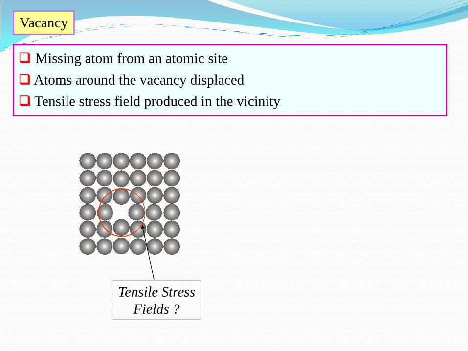
Vacancy

Missing atom from an atomic site

Atoms around the vacancy displaced

Tensile stress field produced in the vicinity

Tensile Stress

Fields ?

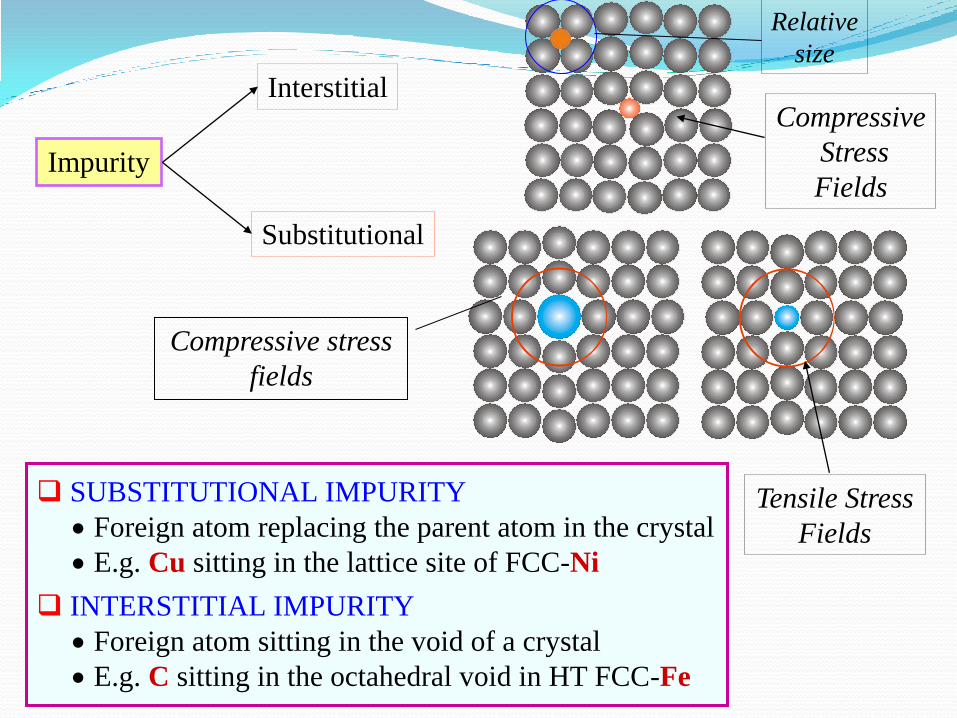
Impurity

Interstitial

Substitutional

SUBSTITUTIONAL IMPURITY

Foreign atom replacing the parent atom in the crystal

E.g. Cu sitting in the lattice site of FCC-Ni

INTERSTITIAL IMPURITY

Foreign atom sitting in the void of a crystal

E.g. C sitting in the octahedral void in HT FCC-Fe

Compressive stress

fields

Tensile Stress

Fields

Compressive

Stress

Fields

Relative

size

Frenkel defect

Cation (being smaller get displaced to interstitial voids)

Pair of anion and cation vacancies

Schottky defect

13

• cause slip between crystal plane when they move,

• produce permanent (plastic) deformation.

Schematic of a Zinc (HCP):

• before deformation • after tensile elongation

slip steps

LINE DEFECTS

Edge Dislocation

An edge dislocation results from a mismatch in the rows of atoms, as if an extra plane of atoms was inserted.

The burger’s vector, b, represents how far we would have to move an atom to bring it back into registry. The burgers vector is perpendicular to the dislocation line.

Screw Dislocation

Screw dislocations result from “shearing” in the crystal. The burgers vector, b, is parallel to the slip plane

Mixed Dislocation

TWIN BOUNDARIES

If the atomic arrangement on one side of a boundary is a mirror reflection of the

arrangement on the other side, then it is called as twin boundary.

16

Grain boundaries:

• are boundaries between crystals.

• are produced by the solidification process, for example.

• have a change in crystal orientation across them.

• impede dislocation motion.

grain boundaries

AREA DEFECTS: GRAIN BOUNDARIES

Whenever the stacking of atomic planes is not in a proper sequence throughout the

crystal, the fault caused is known as stacking fault.

For example, the stacking sequence in an ideal FCC crystal may be described as A-

B-C-A-B-C- A-B-C-……. But the stacking fault may change the sequence to A-B-

C-A-B-A-B-A-B-C. The region in which the stacking fault occurs (A-B-A-B) forms

a thin region and it becomes HCP.

VOLUME IMPERFECTIONS

Presence of a large vacancy or void space, when cluster of atoms are missed is also

considered as a volume imperfection.

STACKING FAULTS


Prepared by

Mukesh kumar

Assistant professor

Darbhanga college of engineering

2

Structures of Metals

Space lattices

Atom presents in any crystalline material are arranged in a regular three dimensional repeating pattern. this pattern is known as space lattice or crystal lattice.

Space latticesThe point of interaction of lines are called lattice point.

Unit cell

A unit cell is the smallest geometrical figure the repetition of which in three dimensions will give the actual crystal structure.

A unit cell is a building block of a crystal. the crystal consist of unit cell of stacked tightly together.

Each identical in shape, size and orientation with each other.

Unit cellA unit cell is completely defined by

six lattice parameters.

a, b, c , a, b, g As shown in figure.

The lattice parameter of a unit cell

are its characteristics intercept

( a, b, c ) and interfacial angles

(a, b, g ) Unit Cells and Unit Cell Vectors

Crystal System

There are seven crystal systems depending upon the lattice parameters of the unit cell.

Each crystal system can be defined in terms of intercepts a, b, c and angles , a, b, g between them.

Many of the seven crystal systems have variations of the basic unit cell.

A French crystallographer A.J. Bravais showed that 14 standard unit cells could describe all possible lattice networks.

Lattice parameter relationship & Figure showing Unit cell Geometries for the seven crystal systems.

Bravais Lattices

Crystal structure for metallic elements

Most metals crystallize in relatively simple crystal structures as under.

Simple cubic Structure

Example –Polonium

Body centred cubic structure (BCC)

Examples –Cr, V, Mo, Mn etc.

Face centred cubic structure (FCC)

Examples –Al, Cu, Ni, Au, Ag, Pb etc.

Hexagonal close-packed (HCP or CPH) structure.

Examples –Mg, Zn, Co etc..

1. Simple cubic structure (SC)

One atom is located at each of the corners of the cube.

Therefore , it contains eight atoms at the corners which are shared by the adjoining eight cubes.

Hence the share of each cube=1/8 th of each corner atom

Total no. of atom/unit cell

=1/8 x 8 corners =1 atom

Atomic RadiusConsidering atoms to be spherical in shape and in contact in a crystal.

Atomic radius can be defined as half the distance between the centers of two neighboring atoms.

Atomic Radius of a Simple Cubic Structure:- In fig. One atom is at each of the corner of

the cube.

If ‘a’ is lattice parameter i.e. length of the cube edge and ‘r’ is the atomic radius. Then,

a=2r

r=a

2

Atomic Packing Factor:-

The packing of atoms in a unit cell of the crystal structure of a material is known as atomic packing.

APF = Volume of atoms in unit cell

Volume of unit cell

16

Atomic Packing Factor of simple cubic structure:-

• APF for a simple cubic structure =p/6 = 0.52

APF = (No. of atoms/unit cell) x (Volume of one atom)

Volume of unit cell

APF = a3

4

3p (0.5a)31

atoms

unit cellatom

volume

unit cellvolumeclose-packed directions

a

R=0.5a

contains 8 x 1/8 = 1 atom/unit cell

2. Body Centred Cubic structure (BCC)

One atom is located at each of the corners of the cube and one atom at the centre of body.

Therefore , it contains nine atoms.2 atoms/unit cell: 1 center + 8 corners x 1/8

Atomic Radius of a BCC Structure:-


From the figure,

AE = AB +BE

= a + a

= 2a

AF = AE +EF

= 2a + a

= 3a

AF = a 3

2 2

2 22

2

2 22

2 2

2

And also,AF =R+2R+R =4R

4R = a 3

R = a 3 4

aR

• APF for a body-centered cubic structure = p3/8 = 0.68

Close-packed directions: length = 4R

= 3 a

Unit cell contains: 1 + 8 x 1/8 = 2 atoms/unit cell

Adapted fromFig. 3.2,Callister 6e.

Atomic Packing Factor of BCC structure:-

APF = a3

4

3p ( 3a/4)32

atoms

unit cell atomvolume

unit cell

volume

3. Face Centred Cubic structure (FCC)

One atom is located at each of the corners of the cube and one atom at the centre of each of the six faces of the cube.

The face centred atom is located at the intersection of the diagonal of the face. 4 atoms/unit cell: 6 face x 1/2 + 8 corners x 1/8

Atomic Radius of a FCC Structure:-


Then considering a triangle,

(4R) = a +a

16R = 2a

R =

2 22

2 2

2 a/4

APF = a3

4

3p ( 2a/4)34

atoms

unit cell atomvolume

unit cell

volume

Unit cell contains: 6 x 1/2 + 8 x 1/8 = 4 atoms/unit cell

a

• APF for a body-centered cubic structure = p/(32) = 0.74

Close-packed directions: length = 4R

= 2 a

Adapted fromFig. 3.1(a),Callister 6e.

Atomic Packing Factor of FCC structure:-

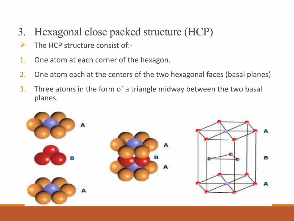
3. Hexagonal close packed structure (HCP) The HCP structure consist of:-

1. One atom at each corner of the hexagon.

2. One atom each at the centers of the two hexagonal faces (basal planes)

3. Three atoms in the form of a triangle midway between the two basal planes.

3. Hexagonal close packed structure (HCP) The unit cell of the HCP contains:-

12 atoms at the corners x 1/6 =2 atoms.

2 face centred atoms x ½ = 1 atom.

3 middle layer atoms = 3 atoms.Total atom in H.C.P. = 6 atoms.

DEFECTS IN CRYSTALS

Point defects

Line defects

Surface defects

Volume defects

0D(Point defects)

CLASSIFICATION OF DEFECTS BASED ON DIMENSIONALITY

1D(Line defects)

2D(Surface / Interface)

3D(Volume defects)

Vacancy

Impurity

Frenkeldefect

Schottkydefect

Dislocation Grainboundary

Twinboundary

Voids / Cracks

Stackingfaults

0D(Point defects)

Vacancy

Impurity

Frenkel defect

Schottky defect

Non-ioniccrystals

Ioniccrystals

Interstitial

Substitutional

Other ~

Vacancy

Missing atom from an atomic site

Atoms around the vacancy displaced

Tensile stress field produced in the vicinity

Tensile StressFields ?

Impurity

Interstitial

Substitutional

SUBSTITUTIONAL IMPURITY Foreign atom replacing the parent atom in the crystal E.g. Cu sitting in the lattice site of FCC-Ni

INTERSTITIAL IMPURITY Foreign atom sitting in the void of a crystal E.g. C sitting in the octahedral void in HT FCC-Fe

Compressive stress fields

Tensile StressFields

Compressive StressFields

Relativesize

Frenkel defect

Cation (being smaller get displaced to interstitial voids)

Pair of anion and cation vacancies

Schottky defect

13

• cause slip between crystal plane when they move,• produce permanent (plastic) deformation.

Schematic of a Zinc (HCP):

• before deformation • after tensile elongation

slip steps

LINE DEFECTS

Edge Dislocation

An edge dislocation results from a mismatch in the rows of atoms, as if an extra plane of atoms was inserted.

The burger’s vector, b, represents how far we would have to move an atom to bring it back into registry. The burgers vector is perpendicular to the dislocation line.

Screw Dislocation

Screw dislocations result from “shearing” in the crystal. The burgers vector, b, is parallel to the slip plane

Mixed Dislocation

TWIN BOUNDARIES

If the atomic arrangement on one side of a boundary is a mirror reflection of the arrangement on the other side, then it is called as twin boundary.

16

Grain boundaries:

• are boundaries between crystals. • are produced by the solidification process, for example. • have a change in crystal orientation across them.

• impede dislocation motion.

grain boundaries

AREA DEFECTS: GRAIN BOUNDARIES

Whenever the stacking of atomic planes is not in a proper sequence throughout the crystal, the fault caused is known as stacking fault.

For example, the stacking sequence in an ideal FCC crystal may be described as A-B-C-A-B-C- A-B-C-……. But the stacking fault may change the sequence to A-B-C-A-B-A-B-A-B-C. The region in which the stacking fault occurs (A-B-A-B) forms a thin region and it becomes HCP.

VOLUME IMPERFECTIONS

Presence of a large vacancy or void space, when cluster of atoms are missed is also considered as a volume imperfection.

STACKING FAULTS

S.No. Name of Student Roll No. Registration No.5

Attendance5

Assignment20

Online_ExamTotal %Marks

1 Prabhat Kumar 18-M-64 18102111001 5 5 20 30 100 Marks Result

2 Aditya Kumar 18-M-67 18102111002 4 5 20 29 96.6666667 Marks<70% 0

3 Shubham Kumar 18-M-11 18102111003 5 5 20 30 100 70%<Marks90% 7

4 Niraj Kumar Gupta 18-M-72 18102111004 5 5 20 30 100 Marks>90% 44

5 Ankush Kumar 18-M-55 18102111005 5 4 17 26 86.66666676 Priya Jha 18-M-04 18102111006 5 5 19 29 96.66666677 Ravindra Kumar Pandit 18-M-53 18102111007 4 5 19 28 93.33333338 Khushbu Kumari 18-M-63 18102111008 4 5 20 29 96.66666679 Chitranjan Kumar 18-M-74 18102111010 5 5 20 30 100

10 Amrit Jeevan 18-M-47 18102111011 5 5 20 30 10011 Indrajeet Gupta 18-M-73 18102111012 4 5 18 27 9012 Amrit Raj 18-M-59 18102111013 4 5 19 28 93.333333313 Vinay Kumar 18-M-61 18102111014 5 5 18 28 93.333333314 Anand Kumar 18-M-22 18102111015 4 5 20 29 96.666666715 Ashok Kumar Mandal 18-M-65 18102111016 4 5 20 29 96.666666716 Nageshwar Kumar 18-M-56 18102111018 5 5 19 29 96.666666717 Swetank Raj 18-M-39 18102111019 4 5 20 29 96.666666718 Vivek Kumar 18-M-12 18102111020 4 5 16 25 83.333333319 Kumar Gaurav Gawaskar 18-M-69 18102111021 4 5 20 29 96.666666720 Sachin Kumar 18-M-16 18102111022 4 5 20 29 96.666666721 Amit Kumar 18-M-15 18102111023 4 5 19 28 93.333333322 Bhaskar Jha 18-M-09 18102111025 4 5 20 29 96.666666723 Satya Kumar 18-M-51 18102111026 5 5 20 30 10024 Ashish Ranjan 18-M-50 18102111028 5 5 20 30 10025 Avkash Kumar 18-M-57 18102111029 5 5 20 30 10026 Shilpi Kumari 18-M-52 18102111032 4 5 20 29 96.666666727 Prabhash Kr. Abhishek 18-M-42 18102111033 4 5 20 29 96.666666728 Prashant Kumar 18-M-45 18102111035 4 5 20 29 96.666666729 Aditya Kumar 18-M-46 18102111036 5 5 20 30 10030 Avinash Kumar 18-M-24 18102111037 4 5 17 26 86.666666731 Aakash Deep 18-M-03 18102111038 5 5 20 30 10032 Jitendra Das 18-M-60 18102111039 5 5 18 28 93.333333333 Sonu Sharma 18-M-35 18102111040 5 5 20 30 10034 Rahul Kumar Sinha 18-M-49 18102111041 5 5 20 30 10035 Shivam Singh 18-M-41 18102111042 5 5 20 30 10036 Md. Tahsirul Ekram 18-M-26 18102111044 4 5 19 28 93.333333337 Shabbir Raza 18-M-62 18102111046 4 4 19 27 9038 Gopal Kumar Prasad 18-M-66 18102111047 4 5 20 29 96.666666739 Amresh Kumar Sahu 18-M-71 18102111048 5 5 17 27 9040 Vivek Kumar Ranjan 18-M-58 18102111049 5 5 20 30 10041 Niraj Kumar 19LEM03 19102111901 5 5 20 30 10042 Ranjan Kumar Mishra 19LEM05 19102111902 5 5 20 30 10043 Md Zakir 19LEM08 19102111903 4 5 19 28 93.333333344 Abhishek Kumar 19LEM10 19102111904 5 5 19 29 96.666666745 Vivek Kumar 19LEM07 19102111905 4 5 20 29 96.666666746 Siddharth Kumar 19LEM02 19102111906 5 5 19 29 96.666666747 Ankit Kumar 19LEM04 19102111907 4 4 19 27 9048 Adarsh Kumar 19LEM01 19102111908 5 5 19 29 96.666666749 Manish Kumar Jha 19LEM11 19102111909 4 5 20 29 96.666666750 Rajeev Ranjan 19LEM09 19102111910 5 5 20 30 10051 Samir Kumar 19LEM06 19102111911 4 5 20 29 96.6666667

Subject (Theory):-Engineering Material

RESULT ANALYSIS

RESULT ANALYSISDarbhanga College of Engineering, Darbhanga

B.Tech - 4th Semester (2018-22), Mechanical Engineering Dept.

0%14%

86%

RESULT ANALYSIS

Result

Marks<70%

70%<Marks90%

Marks>90%

LIST OF STUDENT

S.N. Registration No. Student Name

1 18102111001 Prabhat Kumar

2 18102111002 Aditya Kumar

3 18102111003 Shubham Kumar

4 18102111004 Niraj Kumar Gupta

5 18102111005 Ankush Kumar

6 18102111006 Priya Jha

7 18102111007 Ravindra Kumar Pandit

8 18102111008 Khushbu Kumari

9 18102111010 Chitranjan Kumar

10 18102111011 Amrit Jeevan

11 18102111012 Indrajeet Gupta

12 18102111013 Amrit Raj

13 18102111014 Vinay Kumar

14 18102111015 Anand Kumar

15 18102111016 Ashok Kumar Mandal

16 18102111018 Nageshwar Kumar

17 18102111019 Swetank Raj

18 18102111020 Vivek Kumar

19 18102111021 Kumar Gaurav Gawaskar

20 18102111022 Sachin Kumar

21 18102111023 Amit Kumar

22 18102111025 Bhaskar Jha

23 18102111026 Satya Kumar

24 18102111028 Ashish Ranjan

25 18102111029 Avkash Kumar

26 18102111032 Shilpi Kumari

27 18102111033 Prabhash Kr. Abhishek

28 18102111035 Prashant Kumar

29 18102111036 Aditya Kumar

30 18102111037 Avinash Kumar

31 18102111038 Aakash Deep

32 18102111039 Jitendra Das

33 18102111040 Sonu Sharma

34 18102111041 Rahul Kumar Sinha

35 18102111042 Shivam Singh

36 18102111044 Md. Tahsirul Ekram

37 18102111046 Shabbir Raza

38 18102111047 Gopal Kumar Prasad

39 18102111048 Amresh Kumar Sahu

40 18102111049 Vivek Kumar Ranjan

41 19102111901 Niraj Kumar

42 19102111902 Ranjan Kumar Mishra

43 19102111903 Md Zakir

44 19102111904 Abhishek Kumar

45 19102111905 Vivek Kumar

46 19102111906 Siddharth Kumar

47 19102111907 Ankit Kumar

48 19102111908 Adarsh Kumar

49 19102111909 Manish Kumar Jha

50 19102111910 Rajeev Ranjan

51 19102111911 Samir Kumar

(0206) FACULTY NAME: Mr. Mukesh Kumar Assistant

Documents

Transcript of (0206) FACULTY NAME: Mr. Mukesh Kumar Assistant