
© Yubo Zhou, 2017 - YorkSpace
88
WHAT’S MISSING IN YOUR SHOPPING CART? A SET BASED RECOMMENDATION METHOD FOR ”COLD-START” PREDICTION YUBO ZHOU A THESIS SUBMITTED TO THE FACULTY OF GRADUATE STUDIES IN PARTIAL FULFILMENT OF THE REQUIREMENTS FOR THE DEGREE OF MASTER OF APPLIED SCIENCE OF APPLIED SCIENCE GRADUATE PROGRAM IN ELECTRIC ENGINEERING AND COMPUTER SCIENCE YORK UNIVERSITY TORONTO, ONTARIO JULY 2017
-
Upload
khangminh22 -
Category
Documents
-
view
8 -
download
0
Transcript of © Yubo Zhou, 2017 - YorkSpace

WHAT’S MISSING IN YOUR SHOPPING CART? A SET BASED RECOMMENDATION METHOD FOR”COLD-START” PREDICTION
YUBO ZHOU
A THESIS SUBMITTED TO THE FACULTY OF GRADUATE STUDIESIN PARTIAL FULFILMENT OF THE REQUIREMENTS
FOR THE DEGREE OF
MASTER OF APPLIED SCIENCE OF APPLIED SCIENCE
GRADUATE PROGRAM IN ELECTRIC ENGINEERING AND COMPUTER SCIENCEYORK UNIVERSITY
TORONTO, ONTARIOJULY 2017
© Yubo Zhou, 2017

Abstract
Abstract
A recommendation system recommends items to users based on users’ historical behaviours. This thesis studies
the problem of predicting the missing items in the current user’s session when there is no additional side information
available. We will refer to this problem as “basket recommendation”. In basket recommendation, items belonging to
the same basket do not have spacial dependency. Because of this, temporal recommendation models such as Recurrent
Neural Network and Markov Decision Process do not apply to this type of problem. Many widely adopted basket
recommendation methods such as Matrix Factorization and Collaborative Filtering su↵er from sparsity and scalability
problems.
Furthermore, using only implicit data, many recommender systems fail in general to provide a precise set of
recommendations to users with limited interaction history. This issue is regarded as the “Cold Start” problem and
is typically resolved by switching to content-based approaches which require additional information. In this thesis,
we use a dimensionality reduction algorithm, Word2Vec (W2V, which was originally applied to Natural Language
Processing problems) under the framework of Collaborative Filtering (CF) to tackle the “Cold Start” problem using
only implicit data. We have named this combined method: Embedded Collaborative Filtering (ECF). We conducted
experiments to determine the performance of ECF on two di↵erent implicit data sets. We are able to show that the
ECF approach outperforms other popular state-of-the-art approaches in “Cold Start” scenarios by 2-10% regarding
recommendation precision. In the experiment, we also show that the proposed method is 10 times faster in generating
recommendations comparing to the Collaborative Filtering baseline method.
The experiment results show that the proposed method outperforms baseline methods in ”cold-start” scenarios. In
addition, the proposed method speeds up computation performance. The proposed method enables ”on-line” learning
capability for traditional methods such as ”Collaborative Filtering”. We also apply random sampling and hybrid
methods to further improve the proposed method’s performance. We present empirical results for the proposed method
iv
ii

on public data-sets and compare the proposed method with practical baseline methods. Additionally we also conducted
experiments to analyze hyper-parameters and shared some insights on model behaviours.
v
iii

Acknowledgements
I would first like to thank my supervisor professor Jia Xu of the Department of Electric Engineering and Computer
Science at York University. Professor Xu opened the door of machine learning and recommendation system to me. I
will not come out the idea without his inspiration and help.
I would also like to thank the experts who provided valuable insights and feebacks for this research project: Arman
Akbarian and Maria Angel Marquez Andrade. Without their passionate participation and inputs, the validation and
evaluation experiments could not have been successfully conducted.
vi
iv
Table of Contents
Abstract iv
Acknowledgements vi
Table of Contents vii
Abbreviations 1
List of Tables 2
List of Figures 3
Chapter 1: Introduction 1
Chapter 2: Data Representations And Similarity Measures 4
2.1 Data representations of user behaviours . . . . . . . . . . . . . . . . . . . . . . . . . . . . . . . . . 4
2.2 Similarity measures . . . . . . . . . . . . . . . . . . . . . . . . . . . . . . . . . . . . . . . . . . . . 6
Chapter 3: Proposed Method 8
3.1 Related Works . . . . . . . . . . . . . . . . . . . . . . . . . . . . . . . . . . . . . . . . . . . . . . . 8
3.1.1 Types of feedback . . . . . . . . . . . . . . . . . . . . . . . . . . . . . . . . . . . . . . . . 8
3.1.2 Basket Recommendation and Collaborative Filtering . . . . . . . . . . . . . . . . . . . . . . 9
3.2 Dimensionality Reduction . . . . . . . . . . . . . . . . . . . . . . . . . . . . . . . . . . . . . . . . 12
3.2.1 Item vectors and item representations . . . . . . . . . . . . . . . . . . . . . . . . . . . . . . 12
3.3 Embedded Collaborative Filtering . . . . . . . . . . . . . . . . . . . . . . . . . . . . . . . . . . . . 15
3.3.1 Methodology Overview . . . . . . . . . . . . . . . . . . . . . . . . . . . . . . . . . . . . . 15
3.3.2 System Flowchart . . . . . . . . . . . . . . . . . . . . . . . . . . . . . . . . . . . . . . . . . 16
3.3.3 System overview . . . . . . . . . . . . . . . . . . . . . . . . . . . . . . . . . . . . . . . . . 18
3.3.4 Training Embedding Model . . . . . . . . . . . . . . . . . . . . . . . . . . . . . . . . . . . 21
3.3.5 Embedding Model Inputs/Outputs . . . . . . . . . . . . . . . . . . . . . . . . . . . . . . . . 22
3.3.6 Compute Neighborhood . . . . . . . . . . . . . . . . . . . . . . . . . . . . . . . . . . . . . 23
3.3.7 Item-Item-KNN . . . . . . . . . . . . . . . . . . . . . . . . . . . . . . . . . . . . . . . . . . 23
vii
v
ii
iv
v
iix
ix
x

3.3.8 User-Item-KNN . . . . . . . . . . . . . . . . . . . . . . . . . . . . . . . . . . . . . . . . . 24
3.3.9 Random Sampling . . . . . . . . . . . . . . . . . . . . . . . . . . . . . . . . . . . . . . . . 26
3.3.10 Hybrid Model . . . . . . . . . . . . . . . . . . . . . . . . . . . . . . . . . . . . . . . . . . . 26
3.4 Section Summary . . . . . . . . . . . . . . . . . . . . . . . . . . . . . . . . . . . . . . . . . . . . . 28
Chapter 4: Experiment 29
4.1 Data Sets . . . . . . . . . . . . . . . . . . . . . . . . . . . . . . . . . . . . . . . . . . . . . . . . . 29
4.1.1 Data set properties . . . . . . . . . . . . . . . . . . . . . . . . . . . . . . . . . . . . . . . . 29
4.1.2 Data format . . . . . . . . . . . . . . . . . . . . . . . . . . . . . . . . . . . . . . . . . . . . 29
4.1.3 Online gift store shopping behaviour data set . . . . . . . . . . . . . . . . . . . . . . . . . . 30
4.1.4 MovieLens 100K . . . . . . . . . . . . . . . . . . . . . . . . . . . . . . . . . . . . . . . . . 31
4.1.5 Artificial data set . . . . . . . . . . . . . . . . . . . . . . . . . . . . . . . . . . . . . . . . . 34
4.2 Setup . . . . . . . . . . . . . . . . . . . . . . . . . . . . . . . . . . . . . . . . . . . . . . . . . . . 35
4.2.1 Baseline methods . . . . . . . . . . . . . . . . . . . . . . . . . . . . . . . . . . . . . . . . . 35
4.2.2 Data preparation . . . . . . . . . . . . . . . . . . . . . . . . . . . . . . . . . . . . . . . . . 35
4.2.3 Evaluation Criteria - Precision . . . . . . . . . . . . . . . . . . . . . . . . . . . . . . . . . . 35
4.2.4 Problem Definition . . . . . . . . . . . . . . . . . . . . . . . . . . . . . . . . . . . . . . . . 36
4.2.5 Experiment setup . . . . . . . . . . . . . . . . . . . . . . . . . . . . . . . . . . . . . . . . . 36
4.3 Results . . . . . . . . . . . . . . . . . . . . . . . . . . . . . . . . . . . . . . . . . . . . . . . . . . . 38
4.3.1 Scalability . . . . . . . . . . . . . . . . . . . . . . . . . . . . . . . . . . . . . . . . . . . . 38
4.3.2 Precision . . . . . . . . . . . . . . . . . . . . . . . . . . . . . . . . . . . . . . . . . . . . . 39
4.3.3 Hyper-parameters . . . . . . . . . . . . . . . . . . . . . . . . . . . . . . . . . . . . . . . . . 51
Chapter 5: Conclusion 59
5.1 Contributions . . . . . . . . . . . . . . . . . . . . . . . . . . . . . . . . . . . . . . . . . . . . . . . 59
5.2 Potential uses of the proposed method . . . . . . . . . . . . . . . . . . . . . . . . . . . . . . . . . . 60
5.3 Future Studies . . . . . . . . . . . . . . . . . . . . . . . . . . . . . . . . . . . . . . . . . . . . . . . 61
5.3.1 User profile de-noising . . . . . . . . . . . . . . . . . . . . . . . . . . . . . . . . . . . . . . 61
5.3.2 User embedding model for user-user Collaborative Filtering . . . . . . . . . . . . . . . . . . 62
Biography . . . . . . . . . . . . . . . . . . . . . . . . . . . . . . . . . . . . . . . . . . . . . . . . . . . . 64
Appendices 70
Chapter A: Words Embedding 71
A.1 A probability interpretation of shopping behaviours . . . . . . . . . . . . . . . . . . . . . . . . . . . 71
viii
vi

A.2 Continuous Bag of Words (CBOW) Model . . . . . . . . . . . . . . . . . . . . . . . . . . . . . . . . 72
A.3 Skip-gram (SG) Model . . . . . . . . . . . . . . . . . . . . . . . . . . . . . . . . . . . . . . . . . . 77
ix
vii

Abbreviations
CBF Content Based Filtering.
CBOW Continous Bag of Words nature language model.
CDAE Collaborative Denoising Auto-Encoder.
CF Collaborative Filtering.
ECF Embedded Collaborative Filtering.
iiKNN Item-item Collaborative Filtering.
KNN K-Nearest Neighbours.
LSTBM Long term and short term (hybrid) behaviour model.
LTBM Long term behaviour model.
MF Matrix Factorization.
NLP Nature Language Processing.
POP Popular ranking recommendation method.
SG Skip Gram nature language model.
STBM Short term behaviour model.
SVD Singular Value Decomposition.
uiKNN User-item Collaborative Filtering.
W2V Word to vector embedding method.
1
viii

List of Tables
2.1 Product rating utility matrix . . . . . . . . . . . . . . . . . . . . . . . . . . . . . . . . . . . . . . . . 6
2.2 Product purchase utility matrix . . . . . . . . . . . . . . . . . . . . . . . . . . . . . . . . . . . . . . 6
3.1 Purchase Utility Matrix . . . . . . . . . . . . . . . . . . . . . . . . . . . . . . . . . . . . . . . . . . 9
3.2 new user . . . . . . . . . . . . . . . . . . . . . . . . . . . . . . . . . . . . . . . . . . . . . . . . . . 10
3.3 Product similarity table . . . . . . . . . . . . . . . . . . . . . . . . . . . . . . . . . . . . . . . . . . 11
3.4 Example of transaction history . . . . . . . . . . . . . . . . . . . . . . . . . . . . . . . . . . . . . . 21
4.1 Data-set property . . . . . . . . . . . . . . . . . . . . . . . . . . . . . . . . . . . . . . . . . . . . . 32
4.2 Data-set property . . . . . . . . . . . . . . . . . . . . . . . . . . . . . . . . . . . . . . . . . . . . . 33
4.3 Model settings . . . . . . . . . . . . . . . . . . . . . . . . . . . . . . . . . . . . . . . . . . . . . . . 40
4.4 Model configuration for on-line gift store data-set . . . . . . . . . . . . . . . . . . . . . . . . . . . . 45
4.5 Model configuration for Movielens 100K data-set . . . . . . . . . . . . . . . . . . . . . . . . . . . . 51
4.6 Model configuration of the Movielens 100K data-set . . . . . . . . . . . . . . . . . . . . . . . . . . 53
4.7 Model configuration . . . . . . . . . . . . . . . . . . . . . . . . . . . . . . . . . . . . . . . . . . . . 54
4.8 Model configuration for the Movielens 100K data-set . . . . . . . . . . . . . . . . . . . . . . . . . . 55
4.9 Model configuration for Movielens 100K data-set . . . . . . . . . . . . . . . . . . . . . . . . . . . . 56
2
ix

List of Figures
3.1 Recommendation Flowchart . . . . . . . . . . . . . . . . . . . . . . . . . . . . . . . . . . . . . . . 17
4.1 1st order correlation of On-line gift store data-set . . . . . . . . . . . . . . . . . . . . . . . . . . . . 31
4.2 1st order correlation of Movielens 100K weekly data-set . . . . . . . . . . . . . . . . . . . . . . . . 33
4.3 Response latency for 2k queries, y axis is processing time and x axis is percentage of hidden items . . 38
4.4 Response latency for 20k queries, y axis is processing time and x axis is percentage of hidden items . 39
4.5 Precision@1 of Movielens 100k weekly 90% hidden . . . . . . . . . . . . . . . . . . . . . . . . . . 41
4.6 Precision@1 of Movielens 100k weekly 95% hidden . . . . . . . . . . . . . . . . . . . . . . . . . . 41
4.7 Precision@5 of Movielens 100k weekly 90% hidden . . . . . . . . . . . . . . . . . . . . . . . . . . 42
4.8 Precision@5 of Movielens 100k weekly 95% hidden . . . . . . . . . . . . . . . . . . . . . . . . . . 43
4.9 Precision@1 of Movielens 100k weekly . . . . . . . . . . . . . . . . . . . . . . . . . . . . . . . . . 44
4.10 Precision@3 of Movielens 100k weekly . . . . . . . . . . . . . . . . . . . . . . . . . . . . . . . . . 44
4.11 Precision@5 of Movielens 100k weekly . . . . . . . . . . . . . . . . . . . . . . . . . . . . . . . . . 45
4.12 Precision@1 of on-line gift store 90% hidden . . . . . . . . . . . . . . . . . . . . . . . . . . . . . . 46
4.13 Precision@1 of on-line gift store 95% hidden . . . . . . . . . . . . . . . . . . . . . . . . . . . . . . 47
4.14 Precision@5 of on-line gift store 90% hidden . . . . . . . . . . . . . . . . . . . . . . . . . . . . . . 48
4.15 Precision@5 of on-line gift store 95% hidden . . . . . . . . . . . . . . . . . . . . . . . . . . . . . . 48
4.16 Precision@1 of on-line gift store data-set . . . . . . . . . . . . . . . . . . . . . . . . . . . . . . . . 49
4.17 Precision@3 of on-line gift store data-set . . . . . . . . . . . . . . . . . . . . . . . . . . . . . . . . 50
4.18 Precision@5 of on-line gift store data-set . . . . . . . . . . . . . . . . . . . . . . . . . . . . . . . . 50
4.19 Precision@1 of CBOW model of di↵erent random sampling rate . . . . . . . . . . . . . . . . . . . . 52
4.20 Precision@1 of SG model of di↵erent random sampling rate . . . . . . . . . . . . . . . . . . . . . . 53
4.21 Sensitivity of di↵erent neighbourhood size . . . . . . . . . . . . . . . . . . . . . . . . . . . . . . . . 54
4.22 Precision@1 of di↵erent window sizes . . . . . . . . . . . . . . . . . . . . . . . . . . . . . . . . . . 55
3
x

4.23 Precision@1 of di↵erent models . . . . . . . . . . . . . . . . . . . . . . . . . . . . . . . . . . . . . 56
4.24 Precision@1 of di↵erent CF algorithms . . . . . . . . . . . . . . . . . . . . . . . . . . . . . . . . . 57
4.25 Precision@1 of di↵erent CF algorithms . . . . . . . . . . . . . . . . . . . . . . . . . . . . . . . . . 58
A.1 Continuous Bag of Words model (CBOW) . . . . . . . . . . . . . . . . . . . . . . . . . . . . . . . . 76
A.2 Skip Gram model . . . . . . . . . . . . . . . . . . . . . . . . . . . . . . . . . . . . . . . . . . . . . 78
4
xi

1 Introduction
We will begin by examining the system we are trying to improve. Recommendation systems have now become part
of the core infrastructure of many modern information systems. In many cases they are crucial to the success of com-
panies which base their business decisions exclusively on insights derived from user information. Recommendation
systems are commonly used to improve user experience through personalization and targeting. They are widely used
in all kinds of Internet services. For example, e-commerce platforms use recommendation systems to recommend
products to users based on user’s current and historical shopping intentions and interests; on-line media streaming
platforms, use recommendation systems to recommend movies and music based on user’s preferences; on-line news-
papers and information platforms, use recommendation systems to suggest posts and articles that best match users’
interests.
The main challenges of recommendation systems are:
Scalability Scalability is a common problem in recommendation systems. In memory based recommendation mod-
els, for example, the dimensions of the model’s inputs and outputs grow exponentially as the number of users/items
increases. In such scenarios, when dealing with a large number of items/users, a common solution is to employ a clus-
tering algorithm to section large data sets into smaller sub-clusters and thus build models for those smaller clusters.
The disadvantage of this approach is that sectioning breaks the dependencies and correlations between items from dif-
ferent sub-clusters. The models created by clustering algorithms are unable to learn the global information in the data
and produce biased results George and Merugu 2005. Let us look at an example that demonstrates this problem. If we
have 100 million items and 10 million users in a database, the recommendation system has to make recommendations
based on 100 millions items. One way to make these kind of recommendations is to recommend to users items which
the user had purchased in the past, in this case we need to store ”user bought item X also bought item Y” information
which is a 100 million by 100 million matrix. This large table has two problems, first this table can not be stored in
memory, second the table look up operation is expensive because we have to index 100 million rows or columns of the
table.
1

Sparsity When data is sparse we do not have enough information on items and users for the model to build a
connection to other users and items. A common solution for sparse data is Matrix Factorization Golub and Reinsch
1970. This approach learns the hidden representation of the data. The hidden representation is learned by minimizing
the reconstruction error of regenerated data using the hidden representation (decomposed matrices) of the original data
Koren et al. 2009. The disadvantage of this approach is scalability, as the system has to recalculate USV matrices for
any new item/user in order to compute a prediction for the new item/user. Continuing with previous example, we have
100 million items and 10 million users in the database, nevertheless, it is very unlikely that a user purchased more than
a thousand items, let us say our user only purchased 10 items, if employ the ”user bought item X also bought item Y”
method for recommendation, we would only be able to recommend another 10 items to this user based on this user’s
purchase history.
”Cold-Start” problem refers to the problem that arises when a system does not have enough information on a user
to make high quality recommendations. SVD Golub and Reinsch 1970 (Singular Value Decomposition) is the common
solution for the ”Cold-Start” problem but as mentioned above, current solutions for the ”Cold-Start” problem su↵er
from lack of scalability Golub and Reinsch 1970.
Thesis structure In this thesis we propose a basket recommendation method that addresses the above mentioned 3
problems, this thesis is organized as follows:
In Section 2 we give an introduction to recommendation systems by introducing the data structures and similarity
measures we use in this thesis. In Section 3 we go through related works, where we introduce di↵erent types of
recommendation methods and types of feedback used for recommendation methods. In Section 4 we introduce the
proposed dimensionality reduction method and explain how to apply it to behaviour modelling problems, additionally
we introduce a couple of feature engineering techniques to improve the models performance. In Section 5 we introduce
the modified Collaborative Filtering that combines the proposed dimensionality reduction method and Collaborative
Filtering, we also introduce several extensions for the proposed Collaborative Filtering method to make predictions.
In section 6 we describe the data-sets we used in the experiments and present the data-set properties. In Section 7
we explain the experiment setup and introduce the baseline methods that where compared with our proposed method.
In Section 8 we present the experiment results as well as the analysis of model hyper-parameters. In Section 9 we
summarise the contributions and share some insights of the proposed method as well as list a couple possible directions
of future studies. The details of the dimensionality reduction method are given in the appendix.
Contributions and novelties our contributions and novelties are summarized below:
2

1. The proposed method outperforms baseline methods in ”Cold Start” scenario.
2. Existing state-of-art ”Cold-Start” algorithms are not designed for real-time scenarios, because in order to calcu-
late the recommendations for a new user, existing methods such as SVD have to rebuild the latent representation
of users and items Golub and Reinsch 1970. Our proposed method is able to train the model o✏ine and update
the model online with any new user’s information without recomputing the model (explained in chapter 3.3).
3. Our work introduces a framework for computing recommendations for the ”Cold-Start” scenario where no
auxiliary information is currently available. Existing methods such as Content Based Filtering Pazzani 1999 do
not work in this case because the only information available is implicit transaction data.
4. We introduce the concept of employing existing techniques such as ”Random Sampling” and ”Hybrid Models”
(will be explained in chapter 3.3) to improve our algorithm.
3

2 Data Representations And Similarity Measures
In this section we introduce the data structure we use in the proposed behaviour modelling method. We also introduce
the similarity measures we use in the thesis.
2.1 Data representations of user behaviours
Behaviours can be categorized into two classes, one is basket representation, another class is session representation.
Basket representation stores user behaviours within the same session in an unordered set and it doesn’t preserve the
order of items appearing in the session. On the other hand, the session representation preserves the order of user
behaviours. Thus, session representation is useful for algorithms that rely on order for producing results.
In this thesis we use basket representation, since our algorithm is not time-dependent (thus there is no reliance on
order). Basket representation is a collection of sets of items, items in the same set do not have spacial order, in other
words, the order of items in the same set is ignored.
One-hot Encoding A straight forward approach to represent an item as a vector is call ”one-hot” encoding. ”One-
hot” encoding Wikipedia 2016i is employed to represent a element in the form of histograms. For example, we can
represent a item as a N dimensional vector where the non-zero entry in this N dimensional vector is the index of the
item in the item database.
Let us demonstrate the concept of ”One-hot Encoding” with an example. If we have 3 items in the database with
their names ”laptop”, ”soft drink” and ”fruit”. The indexes of product ”laptop”, ”soft drink” and ”fruit” would be 0, 1,
2 respectively. We can then represent each item as a 3 dimensional vector.
Item ”laptop” becomes:
itemlaptop =< 1, 0, 0 >
Item ”soft drink” becomes:
itemso f tdrink =< 0, 1, 0 >
4

Item ”fruit” becomes:
itemf ruit =< 0, 0, 1 >
Utility vector Now that we have a representation of items. The next step is to use this representation to describe
user behaviours.
If, for instance, the behavioral data is purchase history, let I be the set of unique products in the system, let pi
be the ”one-hot” encoding of product i, then user behaviour can be represented as the set of products this user has
purchased, in the form as a (itemid, count) tuple:
user history =n
(pi, counti), ... , (p j, count j)o
, i, j 2 <I
We can then translate the set members into one-hot encoding vectors pi, where pi is a vector with all entries set
to 0 except entry i where i is the index of item i, so a user profile can be the aggregation of all products this user has
purchased. We can sum all one-hot vectors:
u =PI
i pi
or average the one-hot vectors:
u = 1|I|PI
i pi
In this case, we call u the Utility Vector. For example if a user purchased product ”laptop” once and product ”soft
drink” twice in the past, and the index of product ”laptop” is 0, the index of product ”soft drink” is 1 and the index of
product ”fruit” is 2. Then the utility vector of this user will be:
itemlaptop + itemso f tdrink + itemso f tdrink + itemso f tdrink =< 1, 2, 0 >
Utility Matrix Item transform all user purchase histories in system into utility vectors, and append the utility vectors
together. We get a matrix UM⇥N of all existing users’ behaviors where M is the number of users and N is the number
of items, the i-th row in UM⇥N is the user utility vector, the j-th colomn in UM⇥N is the item utility vector.
We call matrix UM⇥N a Utility Matrix. The entries of a Utility Matrix can consist of purchase counts, ratings,
clicks or keywords, their values can be of two distinct information types:
1. Explicit feedback – feedback such as ratings, user comments and keyword search.
2. Implicit feedback – feedback such as purchase history, like/dislike, and clicks. Note that all implicit feedback is
in binary form.
5

An example of an explicit feedback Utility Matrix is given below:
Table 2.1: Product rating utility matrix
laptop soft drink fruitUser 1 1.0 4.0 1.0User 2 2.0 4.0 1.0
This Utility Matrix represents in the products preferences of two users. User 1 rated product ”soft drink” as 4.0,
product ”fruit” as 1.0 and product ”laptop” as 1.0; user 2 rated product ”soft drink” as 4.0, product ”laptop” as 2.0 and
product ”fruit” as 1.0.
An example of an implicit feedback Utility Matrix is given below:
Table 2.2: Product purchase utility matrix
laptop soft drink fruitUser 1 1 4 1User 2 2 4 1
This Utility Matrix describes the purchase history of 2 users, user 1 purchased 1 ”laptop” product, 1 ”fruit” product
and 4 ”soft drink” products; user 2 purchased product ”laptop” twice, product ”soft drink” 4 times and product ”fruit”
once. In this case the utility vector of user 1 is < 1, 4, 1 >, and the utility vector of user 2 is < 2, 4, 1 >, the utility
vector of product ”laptop” is < 1, 2 >, the utility vector of product ”soft drink” is < 4, 4 > and the utility vector of
product ”fruit” is < 1, 1 >.
Having the Utility Matrix, we can calculate the similarity between two users employing the user row as a feature
vector and calculating the Cosine similarities between the two user vectors. I’ll explain the Cosine similarity in next
section.
2.2 Similarity measures
Similarity measurement is a very common technique used in behaviour modelling. For example, by giving a user’s
purchase history, one can compute the most related items and/or actions based on the given user is purchase history.
The relevance between an user’s behaviour history and items/actions can be interpreted as similarities.
In memory based methods, such as Collaborative Filtering Linden et al. 2003, recommendation methods compute
similarities between items and users to use the similarity scores to calculate recommendations. Model based methods,
such as clustering, however require similarity function to compute the ”relevance score” between items and clusters in
6

order to label item.
Cosine Similarity The similarity function we use in this thesis is cosine similarity. Cosine similarity computes the
normalized dot product between two vectors. Cosine similarity is defined as follow:
s(u, v) =u · vkuk · kvk =
PNi ui · vi
q
PNi u2
i ·q
PNi v2
i
(2.1)
Where u is the utility vector of user/item u = hu1, u2, ..., uni, v is the utility vector of user/item v =
hv1, v2, ..., vni and n 2 <N where N is the number of unique products, ui and vi are the value of i-th entry
of vector u and v respectively.
Cosine similarity calculates the angle between two N-dimensional feature vectors, the result is normalized by the
L2 norm of each feature vector. For recommendation problems, we use Cosine to calculate the similarity between two
users or two items. Users and items can be represented as utility vectors (section 2.1).
Continuing with the example we have used previously, The system has three products: laptop, soft drink and fruit.
We can represent them as a 3 dimensional vector < x, y, z >. Symbols x, y, z represents the purchase behaviour of
product ”laptop”, ”soft drink” and ”fruit” respectively. The value of the i-th entry is 1 if the user purchased the product
and 0 otherwise. Since user1 and user2 purchased product laptop and fruit, the vector representations of user1 and
user2 would be < 1, 0, 1 >, user3 purchased product soft drink, then the vector representation of user3 would be
< 0, 1, 0 >.
In this case the cosine similarity between user1 and user2 would be s(user1, user2) which is 1. The cosine simi-
larity between user1 and user3 would be s(user1, user3) which is 0.
The computational complexity of Cosine is O(n), where n is the dimensions of the utility vector, which is the
number of users or number of unique items in the system. This method scales poorly because of the ”Curse of
dimensionality” Marimont and Shapiro 1979. In real-world scenarios, the dimensions of user’s feature vector may
scale to millions or billions. An online shopping ecommerce platform, for instance, can have millions of products
and users on the platform. In this case the dimension of a recommendation system will be the number of products or
number of users. Thus we need a dimensionality reduction method to reduce these high dimensional features into a
fixed, low dimensional dense features to compute the similarity in a low dimensional space. We go over this in the
”Dimensionality Reduction and Embedding” section.
7

3 Proposed Method
3.1 Related Works
In this section, we will introduce related works of our work. We first explain how do we categorise recommendation
methods. After that we introduce the set based recommendation and session based recommendation. In the end of this
section, we also present some important properties in behaviour modeling problems.
3.1.1 Types of feedback
A recommendation system learns user preferences from behavioural history. This history contains two types of data:
implicit feedback and explicit feedback. Explicit feedback directly records users’ preferences on items. Implicit
feedback requires more analysis as its value is more ambigous.
Explicit feedback Explicit feedback obtained from users indicates a user’s preference. This type of feedback is
defined as explicit only when users know that the feedback provided is interpreted as a preference indicators.
Users may indicate preference explicitly using a binary or graded feedback system. Binary feedback indicates that
a user likes or dislikes a product. Graded feedback indicates a user’s preference of a product on a scale using numbers
(ratings), or descriptions (comments).
For example if a user purchased product ”laptop”, he/she may prefer to leave positive/negative feedback for the
product such as like/dislike. He/she may also leave comments to indicate their preference on the product. Such as
”This is the best flavor I’ve ever tried in my life.” (indicates positive), ”This is the healthiest food I can find in town”
(indicates positive).
Implicit feedback Implicit feedback is inferred from user behavior, such as noting which product they purchased or
did not purchase, the number of repeated purchases, page browsing history and clicks. There are many signals during
the search process that one can use as implicit feedback.
8

For example if a user purchased product ”laptop” 3 times without leaving any explicit feedback, we only know this
user purchased ”laptop”, but we do not have any idea whether this user likes ”laptop” or not, this type of feedback is
known as Implicit Feedback.
3.1.2 Basket Recommendation and Collaborative Filtering
Behavioural models for basket based recommendations rely on the assumption of the behaviours have Markov Property
Durrett 2010. Markov Property means that the future events only depend on the current state and are independent of
the order of historical behaviours. Based on this, users and items in a basket based recommendation system can be
represented as utility vectors.
Let us look at an example that employs Markov Property, for example if an user purchased product ”laptop” 5
days ago and then purchased product ”laptop” again 3 days later. Markov Property means that the future purchase
behaviour of this user only depends on how many ”laptops” this user has purchased in the past. The future purchase
behaviour of this user is unrelated to the order of purchases.
Background The most common approach for recommendation systems is Collaborative Filtering (CF) Linden et al.
2003 which is commonly used by many recommender systems. Collaborative Filtering, also known as K-Nearest
Neighbor search (KNN) utilizes the implicit and explicit feedback given on items by users as the only source of
information. This means that CF mehods do not use any side information to compute the recommendation, examples
of side information are: item description, user meta data, social network information etc.
In this section, I’m going to introduce item-item Collaborative Filtering and explain how to apply them to behavior
modelling problems, in addition I will describe the advantages and disadvantages of CF.
CF computes 3 types of similarities: user-user similarity, item-item similarity and user-item similarity. CF makes
recommendations by predicting the missing values in the Utility Matrix. To illustrate the process, let’s look at some
examples: Scenario 1, we have a utility table of ratings for 4 users and 3 products:
Table 3.1: Purchase Utility Matrix
laptop soft drink fruitUser 1 1 3 ?User 2 ? 2 3User 3 1 3 ?User 4 ? 1 4
And we want to generate a recommendation for the user, the utility vector of this user is given below:
9

Table 3.2: new user
laptop soft drink fruitnew user ? 3 ?
In order to generate a recommendation for the new user, we need to predict the missing value in new user’s utility
vector using the utility matrix of existing users, in this case, existing users are user 1, user 2, user 3, user 4. Since the
new user has never purchased laptop and fruit before, we could recommend laptop or fruit to the new user, but which
product is best to recommend to this user? The answer can be answered by CF.
The most common Collaborative Filtering method is memory based K-Nearest Neighbor (KNN) search. KNN
has two stages, the first stage is to compute the neighborhood of a given item or user; the second stage is to make
predictions using the neighborhood information. We will explain the two stages of recommendation in the next two
sections. In the rest of this thesis, we use KNN and CF interchangeably.
First stage - compute the neighborhood In the first stage, CF computes a neighborhood for a given item, the
neighborhood of the item consists of a set of items sorted by their similarity score. The neighborhood is denoted as
N. In order to calculate the neighborhood, we need to calculate the similarity scores of the item and other items.
There are many ways to calculate similarity scores. In this thesis, we use Cosine Similarity (equation 2.1) to calculate
the similarity score. We employ an utility vector (section 2.1) to represent an item and use it to calculate Cosine
similarities. Let us look at a example that demonstrates how to compute the neighborhood of an item.
Continuing with the example used before, we have 3 products ”laptop”, ”soft drink”, ”fruit” and 4 users user1,
user2, user3 and user4 in the database. The user-product interactions are presented in Table 3.1.
By applying cosine similarity to column ”laptop”, column ”soft drink” and column ”fruit”, we calculate the similar-
ity of products. For example S (”laptop”, ”so f tdrink”) = 1 and S (”laptop”, ” f ruit”) = 0. The reason why similarity
between product ”laptop” and ”fruit” is 0 is because product ”laptop” (< 1, ?, 1, ? >) and product ”fruit” (<?, 3, ?, 4 >)
do not share any non-zero valued entries. We can understand this as: ”users who purchased product ”laptop” never
purchased product ”fruit”, but users who purchased ”laptop” also purchased product ”soft drink”. Based on this shop-
ping behaviour, product ”laptop” is similar to product ”soft drink” compared to the product ”fruit”. thus, the similarity
between product ”laptop” and ”soft drink” is higher than the similarity between product ”laptop” and ”fruit”.
Second stage - prediction In the prediction stage, we look into items that a user has purchased in the past and
then calculate a neighborhood of similar items for all items the user has purchased in the past. We then aggregate all
neighborhoods to generate recommendations. Let us look at an example to demonstrate this process.
10

For example, Table 3.2 represents the shopping history of a user we want to recommend products to. This user
only purchased one item which is product ”soft drink”. The first step is to compute a neighborhood of all purchased
items in other users history (in this case we only need to compute the neighborhood for product ”soft drink”).
Product ”soft drink” is represented as the i-th column in the utility matrix (Table 3.1) where i is the index of product
”soft drink”. In this case it correspondes to the second column in Table 3.1.
Using the utility vector representation for items, we can compute the pair-wise similarities of products in the
system. We store the pair-wise similarities in a table. The similarity table looks as follows:
Table 3.3: Product similarity table
laptop soft drink fruitlaptop 1 1 1soft drink 1 1 0.89fruit 1 0.89 1
If we only recommend 1 product to the new user, we will recommend product ”laptop” instead of product ”fruit”
because based on the behavioural model (similarity table), product ”soft drink” is more similar to product ”laptop”
than product ”fruit”.
Section Summary In this chapter, we introduced the Item-Item Collaborative Filtering method used in the this
work. A concrete description of Item-Item Collaborative Filtering is given in Chapter 3.3. In the next chapter, we will
introduce the dimensionality reduction method we use in the this work.
11

3.2 Dimensionality Reduction
Dimensionality reduction is a common technique used in information system. A dimensionality reduction method
transform vector spaces. In this work we use dimensionality reduction to transform feature vectors from high di-
mensional vector spaces into low dimensional vector spaces. In order to perform dimensionality reduction, we need
to construct a function that takes an N dimensional vector as input and outputs an n dimensional vector where N is
the dimensions of the original vector space and n is the dimension of the embedded space. The information loss is
minimized during dimensionality reduction Hastie et al. 2009. Some particular approaches are even able to learn and
encode extra information from raw data distribution Mikolov et al. 2013. Section 2 describes two representations of
user behaviours (”one-hot” encoding and utility vector) and describes the advantages and disadvantages of those two
representations. In this thesis, we apply unsupervised learning dimensionality reduction to overcome the drawbacks
of one-hot representations.
The idea behind the proposed method is borrowed from the NLP domain Wikipedia 2016h. This method is also
known as Distributive Representation of words, or Word2VecMikolov et al. 2013. This method ”embeds” a discrete
sparse vector space <N into a continuous dense vector space <n where dimensions N � n. We introduce the di-
mensionality reduction method and demonstrate how do we use this dimensionality reduction method for behavioural
modelling in this section.
3.2.1 Item vectors and item representations
Shopping behaviors can be represented as Nth order correlations. In a 1st order correlation, the shopping behaviour
data-set can be represented as a I dimensional vector where I is the number of unique items in the data-set. Each
entry in this vector is the frequency of the item, or how many times this item appears in the data-set. Using a 1st order
correlation, we can represent the shopping behaviour data-set as a I dimensional vector (histogram/utility vector).
As a 2nd order correlation, the item can be represented as an I dimensional vector where each entry of this vector
represents its pair-wise co-appearance frequency in relation to other unique items in the data-set. In this case, the
item-set in the data-set could be a matrix of pair-wise co-appearance frequencies.
As described in section 2.1, a straight forward method for encoding items is ”one-hot” encoding. A ”one-hot”
vector is a vector in a R|V |⇥1 discrete vector space, with one non-zero entry to represent the index of that item and all 0s
for others. Where |V | is the number of unique items in the data-set. The advantage of one-hot encoding is its robustness
and ease of interpretation. The disadvantages of ”one-hot” encoding is that you can not reprsent any inter-correlation
such as a 1st order correlation and a 2nd order correlation. For instance the dot product of any two distinct one-hot
12

vectors is 0. Lets say there are two items in the data-set, one of them is product ”laptop” and another one is product
”fruit”.
wlaptop =
2
6
6
6
6
6
6
6
6
6
4
1
0
3
7
7
7
7
7
7
7
7
7
5
,wf ruit =
2
6
6
6
6
6
6
6
6
6
4
0
1
3
7
7
7
7
7
7
7
7
7
5
the dot product of those two items is:
wB · wA = 0
As we can see, the one-hot encoding does not represent product correlation information. One-hot vector of product
”laptop” is orthogonal to the one-hot vector of product ”fruit”.
The question now becomes: can we transform a ”one-hot” sparse space into a dense, continuous dense space,
based on the fact that we can encode the similarity and any higher order correlation easily using a method such as
cosine similarity, Euclidean distance or Pearson correlation? This ”embedded space” should be able to encode item
correlations in a low and dense dimension space.
Having these questions in mind, we are looking for a mapping function to map a N dimensional vector U into
vector V:
V = (U, ✓), where V 2 <n, U 2 <N and n ⌧ N (3.1)
where ✓ denotes the parameters of mapping function that we are trying to estimate.
For example we have 3 products in the system and they are ”laptop”, ”soft drink” and ”fruit”. The ”one-hot”
encodings of those three products are < 1, 0, 0 >, < 0, 1, 0 > and < 0, 0, 1 > respectively.
Let’s say that mapping function embeds the ”one-hot” embedding vector into a 2-dimensional vector space. By
passing the one-hot encoding to the mapping function, we get:
laptopembed = (laptop, ✓) =< 0.1, 0.9 >
f ruitembed = ( f ruit, ✓) =< 0.3, 0.5 >
so f t drinkembed = (so f t drink, ✓) =< 0.45, 0.51 >
13

We see that the embedded representation of products is no longer ”one-hot” encoding anymore. Using this repre-
sentation, the dot product of any two products will result in a value between -1 to 1. For example, the cosine similarity
between embedlaptop and embed f ruit would be:
S (laptopembed, f ruitembed) = 0.90
Our goal in this thesis is to build the embedding function - equation (3.1) and apply it to convert a products’
”one-hot” encoding into distributive representations. There are many choices to build the embedding function, such
as Jolli↵e 2002, Koren et al. 2009. In this thesis, we choose Word2Vec (Mikolov et al. 2013) for the purpose of
embedding. The main reason we choose Word2Vec for embedding purposes are:
1. Word2Vec embedding is an unsupervised learning method LeCun et al. 2015. Since the data in an implicit
feedback recommendation system Hu et al. 2008 can be considered unlabelled data, we can choose Word2Vec
to learn the item representations from this kind of unlabelled data.
2. Word2Vec is a gradient based optimization method LeCun et al. 2015. This allows ”online learning”, which
means model weights can be updated with individual samples Saad 1998 instead of rebuild the model.
3. Word2Vec embeds items from high dimensional spaces into low dimensional spaces. While speeds up compu-
tation of KNN Keogh and Mueen 2011.
There exist two NLP models used for Word2Vec embedding: Continuous Bag of Words (CBOW) and Skip Gram
(SG). In this thesis, we refer to CBOW as Embedding CBOW and SG as Embedding SGMikolov et al. 2013.
Details about Word2Vec embedding (3.1), CBOW and SG model are given in appendix A.
14

3.3 Embedded Collaborative Filtering
In this thesis, we propose a method which we call ”Embedded Collaborative Filtering” (ECF). We employ the Collabo-
rative Filtering (CF) framework along with the dimensionality reduction method Word2vec, to create recommendations
for “Cold Start” scenarios. This combination is what we name ECF. In this section, we will introduce ECF and explain
how to train embedding models as well as how to apply embedding models in a Collaborative Filtering framework.
In addition, we also introduce several techniques to enhance the embedding model performance of recommendation
problems.
3.3.1 Methodology Overview
Collaborative Filtering has been proven to be a robust recommendation framework Hu et al. 2008. But Collaborative
Filtering su↵ers scalability and sparsity problems Grcar et al. 2005. Collaborative Filtering performs poorly in large
and/or sparse dataset (eg. ”Cold Start” problem).
Methods like Matrix Factorization (MF) Koren et al. 2009 and Singular Value Decomposition (SVD) Golub and
Reinsch 1970 do not work well in real-time scenarios, because MF and SVD calculate recommendations by approx-
imate the missing value in the target user’s transaction profile. The approximation process iterates entire dataset to
calibrate model parameters. This poses a huge computation burden Vavasis 2009 for a real-time scenario.
Another research direction is to use auxiliary information to make recommendations in ”Cold Start” scenarios
(Content Based Filtering - CBF). The limitation of CBF is that CBF calculates item-similarities using item meta data
(eg, descriptions, item features). Because of that, CBF can not make recommendations for shopping intentions. In
addition, to acquire auxiliary information incurs additional cost to the system.
In this work, we combine Collaborative Filtering with unsupervised embedding to address ”cold start” problems in
real time scenarios. The reasons for combining Collaborative Filtering with unsupervised embedding are summarized
below:
1. Collaborative Filtering works with user-item interactions and does not require any additional information
2. W2V embedding method is a gradient based method Mikolov et al. 2013 which allows online learning Bottou
2010. This ensures that the item-item similarity model is up-to-date with the latest interactions.
3. The size of the W2V embedding model is irrelevant to the number of users in the system, this means the size of
the model will not grow through time.
15

4. CF is an neighbourhood based method, the dimensionality of the data is the critical factor improving com-
putational performance. W2V embedding is a dimensionality reduction method, it embeds items from high
dimensionality vector spaces into lower dimensionality spaces. Normally the compression rate ranges between
90%-99%. For example, in the experiment we embed items from an original 3000 dimensional ”one-hot” vector
space into a dense 50 dimensional vector, in this case, the compression rate is (3000-50)/3000 = 98.3% which
significantly improves the CF computing speed.
In next section, we will present the recommendation flowchart and give an end-to-end real world example to help
the reader gain a overview of the system data flow, after that we will explain each component in the system in detail.
3.3.2 System Flowchart
In this section, we present the data flow of the system and explain each component in the system, the system flow chart
is shown in Figure 3.1:
16

Figure 3.1: Recommendation Flowchart
17

There are 8 components in the recommendation pipeline, they define the system’s inputs, outputs and processing
units:
1. System Inputs The system inputs are transaction records. The first step in the system is to convert transactions
into the user sessions (receipts) data structure.
2. Embedding The second step is to embed each item in a user session into an embedded representation. The
next step is to pass the embedded user session into the KNN method. One KNN method used in the system is
User-Item KNN and another KNN method used in the system is Item-Item KNN.
3. User-Item KNN - Aggregate User Session In User-Item KNN (details are given in Section 3.3.8), the KNN
method takes user sessions as input and output recommendations. The first state of the User-Item KNN algorithm
is to average all embedded vectors in a user session into a single embedded vector.
4. User-Item KNN - Compute neighborhood The second step of the User-Item KNN algorithm is to compute a
neighborhood of averaged vector (the details are given in section 3.3.6).
5. Item-Item KNN - Compute Neighborhood Another KNN method used in this work is Item-Item KNN. In the
first step of Item-Item KNN, the system computes a neighborhood for each item in a user session (details are
given in Section 3.3.7).
6. Item-Item KNN - Aggregate Neighborhood In the second step of Item-Item KNN, the system aggregates all
neighborhoods into a single neighborhood. The details of aggregation are given in section 3.3.7 algorithm (2)
(line 10 and line 11)
7. Sort Neighborhood We rank the items in the neighborhood by sorting them based on their similarity scores
8. System Outputs We return the top-n neighbors in the sorted neighborhood as recommendation results
3.3.3 System overview
In this section, we give an end-to-end example that demonstrates the functionality of the proposed system. Let us say
we deployed the recommendation system on an online e-commerce website, and the e-commerce website has 4 items
with 5 historical transactions.
18

Environment-Item Database Let’s define three products A, B and C. The one-hot representations of item A, B and
C are:
1. A - < 1, 0, 0, 0 >
2. B - < 0, 1, 0, 0 >
3. C - < 0, 0, 1, 0 >
4. D - < 0, 0, 0, 1 >
Environment-Historical Interactions Let’s say we have 5 historical transactions (receipts) in the database from 5
di↵erent users:
1. user1: A,C
2. user2: A,C
3. user3: A, B
4. user4: A, B,C
5. user5: A,D
We train the embedding model with receipts (explained later in this section) and embedding dimension 2. After
embedding, the vector representations of item A,B and C become:
1. A - < 0.1, 0.8 >
2. B - < 0.25, 0.91 >
3. C - < 0.35, 0.45 >
4. D - < 0.67, 0.77 >
After this step, we are done with embedding, the next step is to use the embedding model in the CF framework.
19

Aggregate items in a user profile Let’s say we have a new customer shopping on an e-commerce website and added
item A and B into the shopping cart. Once the customer added the items into the shopping cart, the system is going to
make a recommendation for this customer. The recommendation system decided to use User-Item KNN to aggregate
the user profile. In this example, we calculate the average of the embedded representations of items A and B, which
are:
avg(A, B) = avg(< 0.1, 0.8 >, < 0.25, 0.91 >) =< 0.175, 0.855 >
Generate recommendation Once we obtain the user profile vector < 0.175, 0.855 >, we can calculate the neigh-
bourhood of the averaged vector using cosine similarity as a distance function. The list of neighbours we got are
(where first column is item-id, and second column is the similarity):
1. B, 0.9978
2. A, 0.9969
3. C, 0.8964
4. D, 0.8706
From the results we can see that item A and item B are very close to the user profile vector, this makes sense because
the user profile vector is the central point of cluster A,B, which means the averaged vector is sitting in between item
A and B.
Once we get the ranked neighbourhood, we can use the results to make recommendations. Let’s say we only
want to recommend 1 item (top 1 recommendation), there are two ways to do that, if we want to recommend items
that customer already purchased, we can recommend item B because the score of item B is highest. But if we do
not want to recommend items that a customer already purchased, in this case, we will remove item A and item B
from the neighbourhood and than use the the remaining items with highest score as recommendation. Thus we should
recommend item C to this customer.
Update the embedding model with new interactions The new user has produced a new interaction (receipt) which
is item A and B. We train the model with the new receipt. After model update, the item embedded representation
becomes:
20

1. A - < 0.14, 0.85 >
2. B - < 0.27, 0.88 >
3. C - < 0.30, 0.40 >
4. D - < 0.60, 0.77 >
3.3.4 Training Embedding Model
In this section, we explain the procedure to train embedding models and introduce the data structure we use to train
the embedding model. The raw data structure used in this thesis is transaction records. Each record has transaction
related information such as ”user id”, ”item id”, ”quantity”, ”transaction date”. Since the embedding method takes
a list of item IDs as input. We need to convert the transaction history into list of item IDs. We do this by grouping
transactions by user ID. In this thesis, we call a list of itemID a “Receipt”.
Receipts An example of transaction history is given below:
Table 3.4: Example of transaction history
user ID item ID quantity timestampU269 laptop 1 2017-01-01 15:30U269 fruit 2 2017-01-01 15:30U269 soft drink 3 2017-01-01 15:30U114 laptop 1 2017-01-01 18:01U114 fruit 1 2017-01-01 18:01U269 fruit 1 2017-01-02 11:31U269 soft drink 1 2017-01-02 11:31
In this example, we have 2 users (U269, U114) and 3 products (laptop, fruit, soft drink). We also have purchase
quantity and purchase timestamp information for each record. In order to train an embedding model, we aggregate
transaction history to create ”receipts”. A receipt contains all items that are bought together by the same user. In this
case we consider that all transactions which happened at the same time, belonging to the same user and belonging to
the same receipts, as purchased together by that user.
By aggregating the transaction history, we obtain a collection of receipts:
1. laptop, f ruit, so f tdrink
2. laptop, f ruit
21

3. f ruit, so f tdrink
Each receipt is a set of items that were purchased together by the same user. Note that items belonging to the same
receipt do not have spatial orders. The orders presented in this example are arranged arbitrarily.
We use receipts as training data to train the embedding model. The embedding model takes k-items as input and
builds the embedded representation of each item. In this case, we select k items from each receipt and pass them to
the embedding model to train the model in a supervised learning way LeCun et al. 2015. There are two options for
the training objective functionsMikolov et al. 2013, one is called Continues Bag of Words (CBOW) and another one
is called Skip Gram, the detailed explanations of those two training objective functions can be found in Appendix
A.2 and Appendix A.3. The embedding model updates model parameters based on batches of training samples. This
training approach is called “mini batch stochastic gradient descent” LeCun et al. 2015.
3.3.5 Embedding Model Inputs/Outputs
As mentioned in equation (3.1), the embedding model maps a N-dimensional vector into a n-dimensional vector.
Normally n is smaller than N. This embedding model converts ”one-hot” vector representations into dense vector
representations. We define the following concepts of the embedding model:
1. Context Window The model takes k items at a time as inputs, the value k is called context window size. To
train the model using receipts, we have to select k items from a receipt and pass k items to the model at a time.
If a receipt has less than k items, we pass all items in the receipt to the embedding model.
2. Embedded Dimension Embedded Dimension defines the dimension of embedded vectors. For example if the
total number of unique items in the data base is 100, the dimension of “one-hot” encoding will be 100, and we
set the embedded dimension to 3, the embedding model will embeds the 100 dimensional “one-hot” vector into
a 3 dimensional embedded vector.
We build the embedding model with above mentioned two properties. The embedding model takes original ”one-
hot” encoding representation of products as inputs, and outputs the embedded representation.
22

3.3.6 Compute Neighborhood
In this section, we explain how to calculate the neighborhood for step 4 and step 5 in the system flow chart. We use
K-Nearest-Neighbors (KNN) with cosine similarity function (equation 2.1) to calculate the neighborhood. KNN finds
the most similar k data points of given data point, the pseudo code of KNN algorithm is presented in Algorithm 1:
Algorithm 1 KNN1: procedure KNN2: I Item set contains all items3: target The data point we need to find k nearest neighbors4: k number of neighbors5: neighborhood ; (the neighborhood of target point)6: for i in I and i , target do7: neighborhood[i] S(i, target)8: neighborhood sort(neighborhood)[:k]9: return neighborhood
where the similarity function (line 7) S (i, j) is Cosine Similarity (equation (2.1)). The KNN algorithm computes a
neighborhood of given item. The neighborhood is a sorted list of top-k similar items to the given item.
We use KNN in two approaches, one is called “Item-Item-KNN” and another one is called “User-Item-KNN”, we
will introduce these two approaches in next two sections.
3.3.7 Item-Item-KNN
The first approach is called ”Item-Item-KNN” (iiKNN). The input of iiKNN is a receipt (user session), each receipt
contains a set of items this user purchased in the past. The goal of iiKNN is to generate a set of recommendations
for given receipt. In order to do this, iiKNN generates a neighborhood for each item in receipt, once having the set
of neighborhoods, iiKNN aggregates all neighborhoods into one single neighborhood. The final recommendation is
generated from this single neighborhood.
The pseudo-code of iiKNN is presented in Algorithm 2, note that pu in the pseudo code is the receipt of user u,
which is the utility vector of user u; S (i, j) is the Cosine function (equation (2.1)); I is the set of total unique items in
the data base. This algorithm returns a ranked list of items, the items are sorted base on aggregated scores of all items
appears in neighborhoods.
We give an example to demonstrate iiKNN algorithm, for example we have 4 items in the system, ”laptop”,
”soft drink”, ”fruit” and ”bread”. A user purchased product ”soft drink” and ”fruit” in the past, we generate the
neighborhood of product ”soft drink” and ”fruit”, the neighborhood of product ”soft drink” and ”fruit” are given
23

Algorithm 2 Item-Item-KNN1: procedure ItemItemKNN2: rank ;3: n #Neighbors4: k #Recommendation5: for i in pu do6: neighbors ;7: for j in I do8: neighbors[j] S (i, j)9: neighbors sort(neighbors)[:n]
10: for j in neighbors do11: rank[j]+ = neighbors[j]
12: rank sort(rank)[:k]13: return rank
below:
1. ”soft drink”: ”bread” (0.75), ”laptop” (0.6)
2. ”fruit”: ”bread” (0.5), ”laptop” (0.1)
The numbers in the brackets are the pair-wise similarities calculated using equation (2.1). As we see both ”bread”
and ”laptop” appear in the neighborhood of two purchased products. The next step is to aggregate two neighborhoods
into one single neighborhood. To do this, we sum all scores of the same products together (line 10 and line 11). By
doing this, we have a set of products with aggregated scores:
”bread” (1.25), ”laptop” (0.7)
We sort this aggregated score and use the 1st item (top-1 recommendation in this example) for recommendation.
In this case is the product ”bread”.
3.3.8 User-Item-KNN
The second approach is called ”User-Item-KNN” (uiKNN). uiKNN takes a receipt as input. The uiKNN aggregates all
item vectors in the user profile into a single vector. After obtaining the aggregated vector of receipt, uiKNN calculates
a neighborhood of the aggregated vector and generates recommendations from the neighborhood.
There are several choices to aggregate items in a receipt, for example two possible aggregation functions can be
“Average pooling” and “Max/min pooling”.
24

Average pooling Average pooling averages a set of vectors by calculating the average value of each dimension of
given vectors. For example the average vector of two vectors a and b is:
¯a + b = a1+b12 e1 +
a2+b22 e2 + ... +
an+bn2 en
where en is the base vector of the n-th dimension. The aggregated user vector is then used as input of KNN to
calculate the neighborhood.
Max/min pooling Max/min pooling select the max/min value of each dimension in a set of vectors. For example the
max pooling of two vectors a and b is:
max(a + b) = max(a1, b1)e1 + max(a2, b2)e2 + ... + max(an, bn)en
and min pooling of two vectors a and b is:
min(a + b) = min(a1, b1)e1 + min(a2, b2)e2 + ... + min(an, bn)en
where en is the base vector of the n-th dimension. The aggregated user vector is then used as input to the model in
order to calculate the related items.
We give an example to demonstrate how to use average pooling in uiKNN. The average pooling method averages
all items in a receipt (utility vector). For example we have a utility vector < 1, 0, 1, 0 >, which represents the shopping
behaviour of a user. This user profile tells us this user purchased 2 items, one item is the 1st indexed item and another
item is the 3rd indexed item, in this case the 1st entry and 3rd entry of utility vector are set to 1. We know that 1st
indexed item is product ”laptop” and 3rd indexed item is the product ”fruit”. The embedded representation for product
”laptop” and product ”fruit” are < 0.9, 0.31 >, < 0.2, 0.35 > respectively. To represent this user, we average ”laptop”
and ”fruit” embedded vectors:
¯laptop + f ruit = pu =< 0.55, 0.33 >
pu denotes the averaged item vector of the receipt, hence, we can use pu to represent a receipt (user profile/utility
vector). To generate recommendations, we need to compute the neighborhood of pu. In order to do that, we have to
compute the similarities between pu and other products using equation (2.1):
S (pu, ”so f t drink”) = S (< 0.55, 0.33 >, < 0.1, 0.15 >) = 0.905
S (pu, ”bread”) = S (< 0.55, 0.33 >, < 0.3, 0.78) >= 0.788
25

Since product ”soft drink” has higher similarity score compare to product ”bread”, in this case, we recommend
product ”soft drink” to the user u. We have introduced the core algorithm of ECF method which is the iiKNN and
uiKNN, in next section, we will introduce the technique we use in this work to improve the recommendation perfor-
mance.
3.3.9 Random Sampling
The first technique we use to improve ECF performance is called “Random Sampling” Schervish 2012. Random
Sampling is a method to sample items from a given receipt. Since items belong to the same receipt do not have spatial
dependencies/orders. The goal of embedding is to capture all possible co-occurrence patterns of items appear in the
same receipt. There are two ways to do that, one is to use a large context window, but as will be shown in Figure 4.22
in Section 4.3, to use large context window leads to worse model performance. On the other hand, we apply Random
Sampling strategy to sample items in the receipt. The random sampling strategy is defined as follow:
Let l be the length of receipt, which is the number of items in the receipt. Let c be the size of context window used
in embedding model. We random sample c items m times from a receipt and use sampled items as inputs to train the
embedding model. The sampling strategy m is defined below:
m = � ⇤ (l � c), (3.2)
where � is the scalar to control random sampling process and the value of � is chosen empirically. The value m
tells us how many times we need to sample c-random items from the receipts and use them as model inputs to train
the embedding model.
3.3.10 Hybrid Model
n this thesis, we propose a hybrid method to improve the recommendation quality. The idea behind a hybrid method
is to combine recommendation results from di↵erent models to produce a recommendation. In this thesis we propose
the idea of creating models for capturing di↵erent kinds of behaviour. Specifically, we define two models, which we
named Long Term Behaviour Model and a Short Term Behaviour Model. In practice, we do not have to limit the
number of models to 2, we can construct multiple models and combine them as an ensemble method.
26

Long Term Behaviour Model (LTBM) A Long Term Behaviour Model (LTBM) captures users’ long term be-
haviour patterns. Building a LTBM requires training the embedding model on long term user behaviours. The long
term user behaviour data are all historical transactions belong to the same users. In Table 3.4, the long term transaction
of each user will be:
1. laptop, f ruit, so f tdring, f ruit, so f tdrink
2. laptop, f ruit
As we can see, the long term behaviour is the concatenation of all receipts belong to the same user.
Short Term Behaviour Model (LTBM) As already mentioned in section 3.3.4. Similarly, a Short Term Behaviour
Model (STBM) captures users’ short term behaviour patterns. Building a STBM requires training the encoder on short
term user behaviours.
Short term behaviours are behaviours grouped by the user in a fixed time period. For example, in online shopping
behaviour, short term behaviours can be the daily transactions or weekly transactions of a user.
Long Term and Short Term Hybrid Behaviour Model (LSTBM) LSTBM is used to enhance the model perfor-
mance by combining the recommendation results from both long and short term behaviour models. The Long Short
Term Behaviour Model (LSTBM) combines LTBM and STBM in a linear combination, as defined below:
LS T BM = ↵ ⇤ LT BM + (1 � ↵) ⇤ S T BM
where ↵ is a hyper parameter to weight the importance of the two models. In this thesis, ↵ is chosen to be 0.5
empirically. The similarity score of LSTBM becomes the linear combination of the similarity scores of the same
product given by LTBM and STBM.
We will give an example to demonstrate the hybrid model mechanism. For example we have 3 products in the
database and they are: laptop, so f tdrink and f ruit. An user purchased product laptop, we want to make a recommen-
dation to that user base on his purchase history, in this case is the product laptop. We pass the user session to Short
Term Behaviour Model and Long Term Behaviour Model separately. The short term model outputs following results:
1. ( f ruit, 0.4)
2. (so f tdrink, 0.1)
and the Long Term Behavior Model outputs following results:
27

1. ( f ruit, 0.1)
2. (so f tdrink, 0.8)
We aggregate the results using the linear combination of two results, let’s say we choose ↵ = 0.5 as the linear
combination weight, the final results will be:
f ruit = 0.5 ⇤ S T BM + 0.5 ⇤ LT BM = 0.5 ⇤ ( f ruit, 0.4) + 0.5 ⇤ ( f ruit, 0.1) = ( f ruit, 0.25)
similarly, we calculate the combined score of product so f tdrink which is (so f tdrink, 0.45). In this example, the
overall score of so f tdrink (0.45) is higher than f ruit (0.25), so we choose product so f tdrink for recommendation.
3.4 Section Summary
In this section, we introduce the proposed method Embedded Collaborative Filtering (ECF) as well as couple exten-
sions of the ECF to improve the model performance. We also give an overview of the data flow of the system in order
to help reader to gain better understanding of the proposed algorithm. In next section we will introduce the data sets
we use in the experiments.
28

4 Experiment
4.1 Data Sets
In this section we evaluate and analyse the performance of the proposed architecture for di↵erent data-sets, namely:
1. Movielens 100k data-set Harper and Konstan 2016
2. On-line gift store data-set Lichman 2013
3. Artificial data-set
4.1.1 Data set properties
Item utility Item utility is the aggregation of non-zero entries of an item vector in utility matrix. The aggregation
can be average aggregation or summation aggregation. The item utility can be interpreted as the popularity of the item
in the data-set. For example if item A is purchased 1000 times by all users in the data-set, the item utility for item A
is 1000.
User utility User utility is the aggregation of non-zero entries of an user vector in utility matrix. The aggregation
can be average aggregation or summation aggregation. The user utility can be interpreted how active this user is in the
data-set. For example if user A purchased 1000 items in the data-set, the user utility for user A is 1000.
4.1.2 Data format
The raw data are stored in .csv files. A snapshot of transaction history in on-line giftstore data-set is given below:
Listing 4.1: Transaction history example
user ID , i temID , q u a n t i t y , d a t e
101 , A1060 , 1 , 2016�01�01
29

101 , A1061 , 1 , 2016�01�01
102 , A5829 , 1 , 2016�01�01
102 , A6382 , 1 , 2016�01�01
102 , A9402 , 1 , 2016�01�01
101 , A2068 , 1 , 2016�01�02
101 , A3850 , 1 , 2016�01�02
As described in section 3.3.4, the proposed method requires “receipts” data format as inputs. In order to convert
transaction data into receipt data, we group daily transactions belong to the same user together, by doing this, we have
created a collect of receipts:
Listing 4.2: Receipts example
A1060 A1061
A5829 A6382 A9402
A2068 A3850
In the following section, we will introduce the data sets we use in the experiment and share some insights/properties
of the data sets.
4.1.3 Online gift store shopping behaviour data set
Data Set Information This is the data set of a on-line shopping platform Lichman 2013, which contains all the
transactions occurring between 01/12/2010 and 09/12/2011, for a UK-based and registered non-store online retail.
The company mainly sells unique all-occasion gifts. Many customers of the company are wholesalers.
Attribute Information The original data is in csv format, the table consists of the following columns:
1. InvoiceNo: Invoice number. Nominal, a 6-digit integral number uniquely assigned to each transaction. If this
code starts with letter ’c’, it indicates a cancellation.
2. StockCode: Product (item) code. Nominal, a 5-digit integral number uniquely assigned to each distinct product.
3. Description: Product (item) name. Nominal.
4. Quantity: The quantities of each product (item) per transaction. Numeric.
5. InvoiceDate: Invice Date and time. Numeric, the day and time when each transaction was generated.
30

6. UnitPrice: Unit price. Numeric, Product price per unit in sterling.
7. CustomerID: Customer number. Nominal, a 5-digit integral number uniquely assigned to each customer.
8. Country: Country name. Nominal, the name of the country where each customer resides.
In this thesis we use StockCode as item ID, Quantity as quantity, InvoiceDate as timestamp and CustomerID as user
ID. By defining these keys, we create receipts by grouping all SockCode which purchased by the same CustomerID
on the same day. We convert timestamp to date in “YYYY-MM-DD” format.
Item popularity The item utility distribution of this data-set is shown below:
Figure 4.1: 1st order correlation of On-line gift store data-set
from Figure 4.1 we can tell only a small portion of items are popular items (around 200 items), and other non
popular items are purchased by customers less then 200 times.
The data-set properties is given below:
4.1.4 MovieLens 100K
MovieLens data sets were collected by the GroupLens Research Project at the University of Minnesota.
31

Table 4.1: Data-set property
property name valuenumber items 3665number users 16766avg item utility 108.57380627557981avg user utility 23.733925802218778avg item density 0.029624503758684806avg user density 0.0014155985805927936avg (item utility / user utility) ratio 4.57462482946794
This data set consists of:
1. 100,000 ratings (1-5) from 943 users on 1682 movies.
2. Each user has rated at least 20 movies.
There are four columns in rating file:
1. user id
2. item id
3. rating
4. timestamp
Data pre-processing Since the data contains users ratings, it is originally an explicit data. To convert data into
implicit data, we assume that users liked the movies when they gave them rating greater than 3. Hence, we convert
the rating data to 1 if the rating is greater than 3 and remove it if the rating is less or equal to 3.Then, we create a
new data-set from this implicit data by concatenating user-id with week number of the year. By doing this, we have
converted the explicit feedback into implicit feedback and create “receipts”of weekly user behaviours.
The new data-set indicates weekly (short-term) users behaviours toward movies.
32

Item popularity The item utility distribution of this data-set is shown below:
Figure 4.2: 1st order correlation of Movielens 100K weekly data-set
from Figure 4.2 we can tell the 1st order correlation of MovieLens data set is similar to on-line gift store data set,
only a small portion of items are popular items. The most important task for the recommender system is to build the
connections from popular items to non-popular items.
Table 4.2: Data-set property
property name valuenumber items 1447number users 1817avg item utility 38.26814098134071avg user utility 30.475509080902587avg item density 0.026446538342322534avg user density 0.016772432075345397avg (item utility / user utility) ratio 1.2557014512785074
33

4.1.5 Artificial data set
In order to better understand the performance of proposed method, we implemented a simulation engine to generate
artificial data.
Configurations The simulation engine generates artificial data with the following configurations:
1. Number of users
2. Number of items
3. 1st order correlation
4. 2nd order correlation
5. Edors Renyi/Exponential/Gaussian distribution
We can generate artificial transaction data for given configurations, for example, if we want to generate a artificial
data set with 1000 users and 10000 items where 1st order correlation and 2nd order correlation in Normal Distri-
bution, we can pass these configurations to the data generator and it will generate artificial transactions base on the
configurations.
We will present the experiment setup and explain how we evaluate proposed method in the next section.
34

4.2 Setup
In order to demonstrate the advantages of the proposed behaviour modelling method, we will conduct a set of experi-
ments that compare the prediction precision between ECF and baseline methods.
4.2.1 Baseline methods
We compare the proposed method with three baseline methods, they are:
1. Collaborative De-noising Auto Encoder (CDAE) The CDAE Wu et al. 2016 is the state-of-art basket recom-
mendation method. CDAE is a deep learning based Collaborative Filtering algorithm, it uses de-noising auto
encoder architecture to learn the purchase sequence from users.
2. Item-Item Collaborative Filtering (iiCF) iiCF Sarwar et al. 2001 is the most common basket recommendation
method for both implicit feedback and explicit feedback.
3. Popularity ranking (POP) POP is the most common and simple recommendation method for ”Cold-Start”
scenario. POP constructs a popularity (1st order correlation) list of items of the data-set and use the top-k most
popular items for recommendation.
4.2.2 Data preparation
In this thesis, we only focus on predicting short-term behaviours. The short term behaviours are defined as a set
of interactions performed together. In this work, regarding to on-line shopping behaviour, we define the short-term
behaviours as a list of items purchased together by the same customer, in other words, items appear on the same receipt.
All transactions happen in the same time with the same customer ID are considered belong to the same receipt. In
movie watching behaviour, we define short term behaviour as short term movie preferences. This reflects on short
term movie rating patterns, such as weekly movie rating patterns and monthly movie rating patterns. We create the
above mentioned data by grouping interactions by the same user within a fixed time period. In on-line shopping data,
we group transactions of the same user happened in the same time together to create receipt. In MovieLens data set,
we group movie ratings rated by the same user within one week in to create weekly movie preference.
4.2.3 Evaluation Criteria - Precision
Precision indicates the size of the fraction of the retrieved information to the relevant information. The formula to
calculate precision is given below:
35

precision = |sreT
srt ||sre |
where sre is the set of relevant information and srt is the set of retrieved information.
4.2.4 Problem Definition
Precision We have created a testing scenario for the precision evaluation. The testing scenario for precision is
to predict removed items from a given user session. The user session can be receipt or movie preference. In on-line
shopping data-set, we random remove items from a receipts and use recommendation system to predict removed items;
in MovieLens data-set, we random remove movie ratings from weekly movie rating patterns and use recommendation
system to predict removed ratings.
Scalability Scalability is a way to measure how well a system performs when amount of work grows Wikipedia
2017. In order to meet real-time requirement, the system has to return the results within a given time interval. To mea-
sure the scalability of recommendation system, we test recommendation system with di↵erent work loads and record
the response time. For example, the response time to answer 2k queries and 20k queries. The scalable recommendation
method should take less time to response queries compare to baseline methods across all work loads.
4.2.5 Experiment setup
The experiment is setup as follows:
Two subsets are randomly selected from samples with a ratio r. One is selected for training and another one is
selected for testing. Let Tr denotes training set and Te denotes testing set. Ratio r is given by:
r = |Tr ||Te |+|Tr |
The models are trained with training set Tr and the results are evaluated using test set Te. In this experiment, r is set to
0.8. During the testing phase, each testing sample is shu✏ed and divided into two parts with a predefined ratio rt. Let
Tq represents the first part, let Th represents the second part. Tq is used as query to query the recommendation system,
Th is used to validate the recommendation results. We call Th hidden items.
The ratio rt is called hidden ratio and defined by:
rt =|Tq||Tq|+|Th |
.
36

In the experiment, 11 di↵erent hidden ratios are used. They are 5%, 10%, 20%. 30%, 40%, 50%, 60%, 70%, 80%,
90%, 95%; hidden ratios 95%, 90% are considered as ”Cold-Start” scenario because there are very few items available
in recommendation query. Each test scenario runs 100 times with random initialization, the experiment results are
averaged from 100 experiments results.
37

4.3 Results
In this section we compare the proposed method with baseline methods in two aspects: query time and precision.
4.3.1 Scalability
We explained how to measure system scalability in Section 4.2.4. In the scalability test, we created two artificial data
sets, the 1st data set contains 10k users and 1k items, the second data set contains 10k users and 10k items.
Figure 4.3: Response latency for 2k queries, y axis is processing time and x axis is percentage of hidden items
Figure 4.3 shows the response latency of processing 2k queries in artificial data with 10k users and 1k items.
The algorithms used in this experiment are user-item Embedded Collaborative Filtering and item-item Collaborative
Filtering.
In this experiment, we compared proposed method (ECF) with item-item Collaborative Filtering (iiCF) with re-
sponse latency metric. The result shows that the response time of proposed method doesn’t increase as much as iiCF
when the length of user profile increases. The response latency of proposed method outperforms iiCF in ”cold-start”
and non-”cold-start” scenarios (hidden ratios from 90% to 10%).
38

Figure 4.4: Response latency for 20k queries, y axis is processing time and x axis is percentage of hidden items
Figure 4.4 shows the response latency of processing 20k queries of artificial data with 10k users and 10k items.
The algorithms used in this experiment are user-item Embedded Collaborative Filtering and item-item Collaborative
Filtering. In this experiment, items are embedded into 30 dimensional embedded space.
In this experiment, we compared proposed method (ECF) with item-item Collaborative Filtering (iiCF) with re-
sponse latency metric. The result shows that the response time of proposed method doesn’t increase as much as iiCF
when the length of user profile increases. The response latency of proposed method outperforms iiCF in ”cold-start”
and non-”cold-start” scenarios (hidden ratios from 90% to 10%). The result is consistent across di↵erent size of
data-set (from 1k item-10k user to 10k item-10k user).
4.3.2 Precision
In this section we will compare The prediction precision of di↵erent methods in two data-sets introduced in Section
4.1. The test scenario is described in Section 4.2.4.
There are two options for Word2Vec objective functions, one is called Continuous Bag of Words (CBOW) and
another one is Skip Gram (SG). The di↵erence between them is they use di↵erent objectives in objective function
LeCun et al. 2015, the detailed explanations of those two training objective functions can be found in Appendix A.1.1
39

and Appendix A.1.2. We refer Embedding model trained with CBOW objective function as Embedding CBOW and
refer Embedding model trained with SG objective function as Embedding SG.
We run each experiment 100 time. During each run, the training and testing set are randomly selected from original
data. Models are trained and tested on the random generated training and testing sets.
During the testing phase, we randomly remove items from each user sessions and use remaining items as query.
We use query to predict random removed items. We will present the comparison results in the rest of this section.
Movielens 100K The settings of the SG and CBOW embedding models for Movielens 100K data-set are given in
table 4.3:
Table 4.3: Model settings
SG CBOWEmbedding model short term short termCF algorithm user-item user-itemEmbedding dimension 40 40Window size 5 5Random sampling rate 0.5 1Number neighbours 10 10
The precision@1 results of 90% hidden rates and 95% hidden rates are presented in Figure 4.5 and Figure 4.6:
40

Figure 4.5: Precision@1 of Movielens 100k weekly 90% hidden
Figure 4.6: Precision@1 of Movielens 100k weekly 95% hidden
41
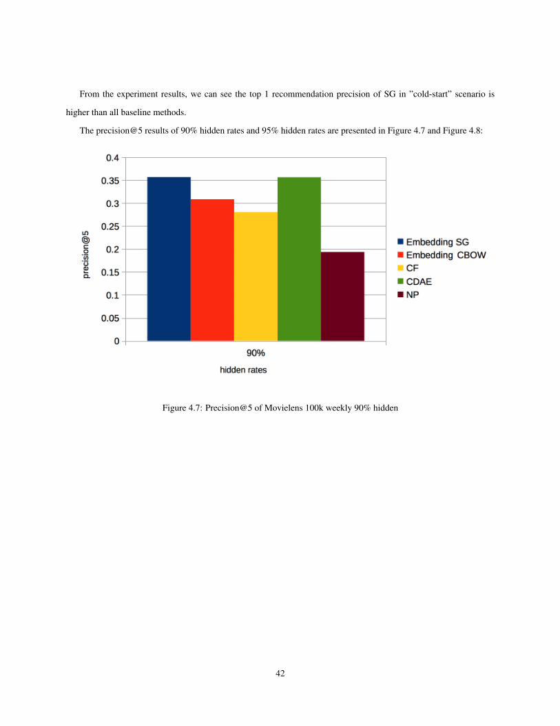
From the experiment results, we can see the top 1 recommendation precision of SG in ”cold-start” scenario is
higher than all baseline methods.
The precision@5 results of 90% hidden rates and 95% hidden rates are presented in Figure 4.7 and Figure 4.8:
Figure 4.7: Precision@5 of Movielens 100k weekly 90% hidden
42
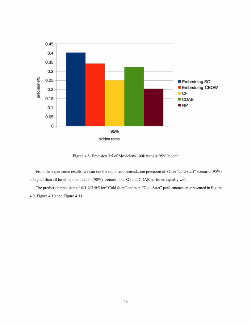
Figure 4.8: Precision@5 of Movielens 100k weekly 95% hidden
From the experiment results, we can see the top 5 recommendation precision of SG in ”cold-start” scenario (95%)
is higher than all baseline methods, in (90%) scenario, the SG and CDAE performs equally well.
The prediction precision of @1 @3 @5 for ”Cold Start” and non-”Cold Start” performance are presented in Figure
4.9, Figure 4.10 and Figure 4.11:
43

Figure 4.9: Precision@1 of Movielens 100k weekly
Figure 4.10: Precision@3 of Movielens 100k weekly
44

Figure 4.11: Precision@5 of Movielens 100k weekly
The x-axis is the percentage of removed items in a user session and the y-axis is the prediction precision.
From the results of the Movielens 100K data-set we can tell the proposed method outperforms baseline methods
in ”Cold-Start” (90%-95% hidden items) scenarios. Proposed method with Skip Gram embedding model outperforms
baseline methods when 80%-95% of items are hidden. The Skip Gram embedding model also outperforms CBOW
embedding model in overall.
On-line gift store The settings of SG and CBOW embedding models for the on-line gift store data-set are given in
Table 4.4
Table 4.4: Model configuration for on-line gift store data-set
SG CBOWEmbedding model short term short termCF algorithm user-item user-itemEmbedding dimension 70 70Window size 5 5Random sampling rate 0.5 1Number neighbours 10 10
45

The precision@1 results of 90% hidden rates and 95% hidden rates are presented in Figure 4.12 and Figure 4.13:
Figure 4.12: Precision@1 of on-line gift store 90% hidden
46

Figure 4.13: Precision@1 of on-line gift store 95% hidden
From figure 4.13 and figure 4.12 we can see that proposed method outperforms baseline method in ”cold-start”
scenario. Interestingly CF performs better than CDAE, maybe because the dataset is sparse.
The precision@5 results of 90% hidden rates and 95% hidden rates are presented in Figure 4.14 and Figure 4.15:
47

Figure 4.14: Precision@5 of on-line gift store 90% hidden
Figure 4.15: Precision@5 of on-line gift store 95% hidden
48

We see consistent results from figure 4.15 and figure 4.14. At top 5 recommendation, the proposed method out-
performs all baseline methods. CBOW outperforms SG model in this experiment.
The prediction precision of @1 @3 @5 for ”Cold Start” and non”Cold Start” are presented in Figure 4.16, Figure
4.17 and Figure 4.18:
Figure 4.16: Precision@1 of on-line gift store data-set
49

Figure 4.17: Precision@3 of on-line gift store data-set
Figure 4.18: Precision@5 of on-line gift store data-set
50

The x-axis is the percentage of removed items in a user session and the y-axis is the prediction precision.
The results of the on-line gift store data-set are consistent with Movielens 100K data-set. The ECF outperforms
baseline methods in ”Cold-Start” scenarios. Interestingly CDAE works poorly in the gift store data-set, we think the
reason for this is the user density of gift store data-set (0.001) is much lower than the Movielens 100K data-set (0.02).
This means that the gift store data-set is sparser than the Movielens 100K data-set and the auto encoder has problems
handling sparse data even though we tried L1 norm as the objective function.
4.3.3 Hyper-parameters
In this section, we present the results for di↵erent choices of hyper-parameters.
Sensitivity of Random Sampling The configurations of SG and CBOW embedding models for the Movielens 100K
data-set are given in Table 4.5:
Table 4.5: Model configuration for Movielens 100K data-set
CBOWEmbedding model short termEmbedding dimension 40Window size 5Random sampling rate -Number neighbours 10CF Algorithm user-item
The prediction precision of CBOW model with di↵erent random sampling rates are given in Figure 4.19:
51

Figure 4.19: Precision@1 of CBOW model of di↵erent random sampling rate
Numbers on right side represents the percentage of removed items, the values of x-axis are choices of random
sampling rates and the values of y-axis are prediction precision.
From figure 4.19 we can see that the recommendation performance improves when random sampling is applied.
The system performance also improves when higher sampling rates applied.
The prediction precision of SG model with di↵erent random sampling rates are given in Figure 4.20:
52
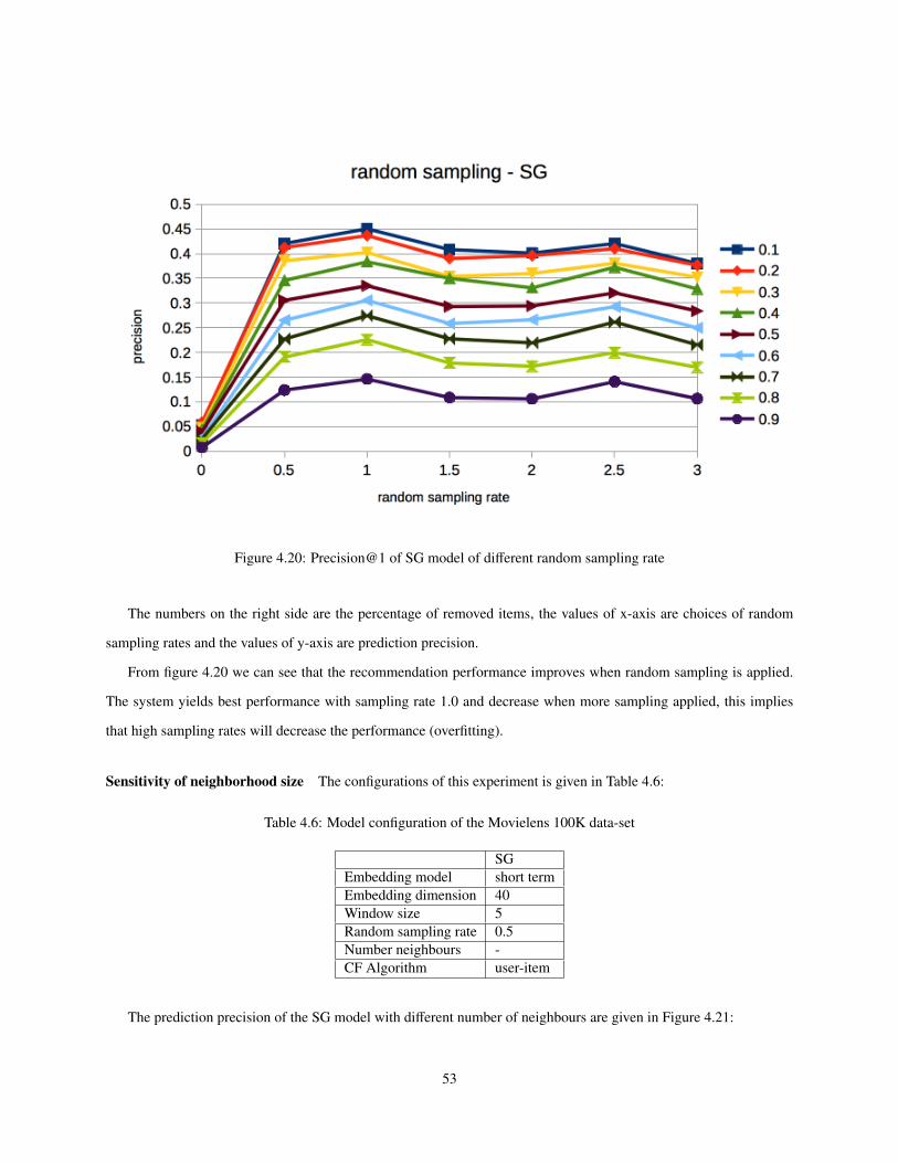
Figure 4.20: Precision@1 of SG model of di↵erent random sampling rate
The numbers on the right side are the percentage of removed items, the values of x-axis are choices of random
sampling rates and the values of y-axis are prediction precision.
From figure 4.20 we can see that the recommendation performance improves when random sampling is applied.
The system yields best performance with sampling rate 1.0 and decrease when more sampling applied, this implies
that high sampling rates will decrease the performance (overfitting).
Sensitivity of neighborhood size The configurations of this experiment is given in Table 4.6:
Table 4.6: Model configuration of the Movielens 100K data-set
SGEmbedding model short termEmbedding dimension 40Window size 5Random sampling rate 0.5Number neighbours -CF Algorithm user-item
The prediction precision of the SG model with di↵erent number of neighbours are given in Figure 4.21:
53

Figure 4.21: Sensitivity of di↵erent neighbourhood size
The values of x-axis are number of neighbours in the neighborhood (size of neighborhood) in KNN and the values
of y-axis represent the recommendation precision. From this results we can see that ECF prediction precision are
persistent with neighborhood sizes.
Sensitivity of Context Window Size The configurations for the SG embedding model with di↵erent context window
sizes are given in Table 4.7:
Table 4.7: Model configuration
SGEmbedding model short termEmbedding dimension 40Window size -Random sampling rate 0.5Number neighbours 1CF Algorithm user-item
The prediction precision of the SG model with di↵erent window sizes are presented in Figure 4.22:
54

Figure 4.22: Precision@1 of di↵erent window sizes
The x-axis is the window size and the y-axis is the prediction precision. From the results we can see both small
and large window size lead to worse performance. Window size between 3-8 yield best performance.
Table 4.8: Model configuration for the Movielens 100K data-set
SG SGEmbedding model short term long termEmbedding dimension 40 40Window size 5 10Random sampling rate 0.5 1Number neighbours 1 1CF Algorithm user-item user-item
Short term/long term models The precision comparisons between hybrid model and single model are presented in
Figure 4.23:
55

Figure 4.23: Precision@1 of di↵erent models
The x-axis is the percentage of removed items in a user session and the y-axis is the prediction precision. From the
results we can see that hybrid and long term model yield better performance in non-”Cold Start” scenarios and hybrid
model is slightly better then long term behaviour model.
Table 4.9: Model configuration for Movielens 100K data-set
user-item CF item-item CFEmbedding model short term short termEmbedding dimension 40 40Window size 5 5Random sampling rate 0.5 0.5Number neighbours 1 1Number queries 200 200
User-Item CF and Item-Item CF The prediction precision of the SG model with di↵erent CF algorithms are given
below:
56

Figure 4.24: Precision@1 of di↵erent CF algorithms
The x-axis is the percentage of removed items in a user session and the y-axis is the prediction precision. From the
result we can see that the performance of user-item CF (centroid point) is better than item-item CF.
It’s also worth mentioning the di↵erences in computation speed of the two CF algorithms:
57

Figure 4.25: Precision@1 of di↵erent CF algorithms
The x-axis is the percentage of removed items in a user session and the y-axis is the computation time (seconds)
to process queries.
Since the user-item CF is to calculate the neighbourhood of averaged vector (centroid point), the recommenda-
tion is the neighbourhood of the averaged vector, so the time to the recommendation is constant. But the time to
compute recommendation scales linearly with number of items in the user profile. Because KNN has to calculate a
neighbourhood for every item in the user profile.
58

5 Conclusion
5.1 Contributions
In this thesis, we proposed a new recommendation method called ”Embedded Collaborative Filtering” (ECF). The goal
of ECF is to improve the recommendation system’s performance in two aspects: recommendation quality (precision)
and scalability.
The main goal of this thesis is to improve recommendation quality (recommendation precision) in ”cold start”
scenarios (when no auxiliary information is available). The experimental results showed that, the recommendation
precision of the proposed is 2% - 10% higher than baseline methods.
In addition, we also experimented with ”random sampling” and the ”hybrid method” to further improve recommen-
dation performance. The ”random sampling” improves ECF recommendation performance by 1% - 5% in ”Cold-Start”
scenarios. The ”hybrid method” improves recommendation performance by 1%-3% in ”non Cold-Start” scenarios.
An additional important di↵erence between the proposed method and existing ”cold start” recommendation meth-
ods is that the proposed method is designed for real-time scenarios. Real-time environments establish constrains for
two critical operations: model updating and recommendation generation. The experiment results show that the time
taken for ECF to generate recommendation is about 10 times faster compared to Collaborative Filtering when the
embedded dimension is set to 1/10 of the original dimension.
Methods like Matrix Factorization (MF) Koren et al. 2009 and Singular Value Decomposition (SVD) Golub and
Reinsch 1970 do not work well in real-time scenarios, as MF and SVD calculate recommendations by approximating
the missing value in the target user’s transaction profile. The approximation process iterates over entire datasets to
calibrate model parameters. This places a huge computational burden Vavasis 2009 for a real-time scenario.
We can avoid this overhead by reusing the models. In ECF, we use pre-trained embedding models to embed items
belonging to a user into embedded vector spaces. After embedding, we aggregate embedded item representations and
then apply KNN on the aggregated user profile to generate recommendations.
In order to evaluate the scalability of the proposed method, we compared the time to generate recommendations
59

between the proposed method and baseline methods on two artificial data-sets. The experimental results showed that
the proposed method takes less time to process recommendation queries for both data-sets.
To summarize:
1. The proposed method is designed for a practical scenario where most of the queries are generated by new users.
This is very common in both ”online” shopping scenarios and ”o✏ine” shopping scenarios.
2. The experimental results show that recommendation quality (precision) of the proposed method outperforms
baseline methods in ”cold-start” scenarios when no auxiliary information is available.
3. The proposed method also improves the computational speed of traditional recommendation methods such as
”Collaborative Filtering”. This is due to the fact that the proposed method reduces the dimensionality of the
original data and employs the reduced dimensional spaces to calculate recommendations.
4. We proposed several techniques to improve the proposed method’s performance such as random sampling and
long/short term behaviour models.
5. We conducted experiments to analyze hyper-parameters and shared some insights on model tuning.
5.2 Potential uses of the proposed method
From the experimental results, we observed that the proposed algorithm outperforms baseline methods in ”Cold-Start”
scenarios, including state-of-art recommendation algorithms.
The proposed method has many potential use cases, Let us elaborate on a couple of possible use cases as follows:
On-line model In the context of retail and e-commerce we purchased multiple items within one shopping session,
this purchase behaviour is then reflected as purchased items in a receipt. Due to privacy issues, we cannot obtain
the user ids from the purchase history. Thus what we end up obtaining is a large volume of short term shopping
behaviours, which are the receipts. In this case we cannot use Collaborative Filtering directly, because there are too
many short term behaviours (user profiles) in the system, which significantly slows down the training process.
What we are looking for is an incremental model that is able to update the model with high volume new shopping
behaviours. By using the proposed behaviour modelling method, we can pre-train the behavioural model with existing
data and then update the model with every new receipt in 1 iteration. By doing this, we can have a on-line model that
is updated with the most recent transactions.
60

Early stage user behaviour intervention Continuing with the retail shopping example, in retail shopping, users
normally purchase a fixed amount of items for each shopping session. For instance, people who purchased 10 items
in the grocery store during one visit are more likely to purchase around 10 items on their next visit. In this case, it
is critical to identify the user’s shopping behaviours at the beginning of the shopping session. By doing this, we can
intervene early in the shopping behaviours of user’s with high conversion rates (”Cold-Start” prediction).
For example, if a shopper added ”soft drink” and ”fruit” to her/his shopping cart, we can guess that maybe the
shopper is preparing a party. In this case, the model tells us this shopper has a high probability of buying ”party
supplies”. Consequently, the business owner can recommend ”on sale” products and products with high profit to the
shoppers with high conversion rates. This early state intervention can also lead to user adoption of new products.
5.3 Future Studies
5.3.1 User profile de-noising
During the experiments, we noticed that sometimes using a sub-set of a user’s profile as query yields better results
compared to using the complete user profile. This may be the main reason why the performance of the proposed
method is worse than other baseline methods in non-”Cold Start” scenarios, since a full user profile contains noise.
We could, however, build a de-noising filter to filter the noise in a long user-profile. By employing any of the
following filters:
1. Sliding window
2. Regression
3. Non-linear regression
Sliding window is a common technique in Collaborative Filtering. A time-dependent sliding window, for instance,
only selects the most recent k transactions to build the user’s utility vector.
Regression uses a weighted vector as filter to filter out the noise. The de-noised user profile can be obtained by
computing the element-wise product between the filter vector and user profile vector.
We want to build a noise filter model for the user profile in a supervised learning fashion. In order to do that,
we need to construct the training samples for supervised learning. The training samples being de-noised user profiles.
One way to construct the training samples is finding the optimal de-noised user profile which leads to highest precision
using Collaborative Filtering.
61

We can also use an optimization method to find the optimal de-noised user profile for each user vector.
Once we obtain the de-noised user profile, we can use regression to learn the de-noising vector.
Non-linear regression employs a non-linear method to build the de-noising vector. A non-linear method could be,
for instance, de-noising Auto Encoder.
5.3.2 User embedding model for user-user Collaborative Filtering
The dimensionality reduction method used in this thesis embeds items from an original vector space to an embedded
space. The drawback of this embedding model is that when the dimension of the sparse vector space changes the
embedding function has to be recomputed. This is why we use an embedding method to embed items in this thesis,
because in a real-world scenarios the item set is less likely to change compared to the user set.
Let us say for example, that we want to build a behaviour model for a web-site to predict a web-site’s visitor
behaviours, the user-item interaction would then become user-web page interaction. The user profile would be the
browsing history of that user. If we built an embedding model from the user distribution to encode user profiles (that
means we train the embedding model on the item utilities), we would face a problem: that we cannot represent new
users using the trained embedding model. Because the embedding model only learns the embedded representation of
existing users based on their browsing history, for any new user with di↵erent browsing history, we would need to
build a new embedding model to encode the unseen browsing history.
Nevertheless, the category of web pages does not change very often. In this case we can train an embedding model
for web page categories, and then use the trained model for any new users with di↵erent browsing histories.
Sequential data and session data Di↵erent solutions have been proposed to encode sequential data with a fixed size
content window. For example Hidasi et al. 2015 formulates the recommendation problem as a sequential prediction
problem and uses a recurrent neural network to generate the prediction.
This kind sequential prediction formulation, however, does not apply to all scenarios. For example, if our problem
is to predict the next receipt using historical receipts. The items in one receipt do not have a specific order. In this case
the sequential based prediction model is hardly working because we cannot pass the unordered items to the model
with arbitrary orders. As any arbitrary ordering will destroy the order dependencies.
In order to address the above mentioned problem, we need a model that is able to process the inputs without
destroying the original orders. One candidate solution is to employ a histogram for representing an unordered set.
As we know, the utility matrix and utility vectors have a histogram structure. Instead of breaking the histogram
into ordered sequential data, we can just embed the utility matrix and utility vectors directly.
62

Embedding method An example of an embedding method is Auto Encoder. We can use the Auto Encoder architec-
ture to learn the latent representations of user profiles, by reconstructing the utility matrix and utility vectors employing
a minimized reconstruction error objective function.
By having a lower dimension representation of a user profile, we can define a new similarity function that computes
the cosine similarity of two users using the embedded representation. The next step is to compute the neighbourhood
of the user profile with the new similarity function.
Challenge of sparsity The challenge of this approach is sparsity, as the density of the utility matrix and utility vector
is very low (in most cases the density is lower then 5%). It is very hard for the auto encoder to reconstruct the inputs.
63

Bibliography
Acquire Valued Shopper Challenge (2014). url: https://www.kaggle.com/c/acquire-valued-shoppers-
challenge/data.
Acquire Valued Shoppers Challenge (2014). url: https://www.kaggle.com/c/acquire-valued-shoppers-
challenge/data.
Adams, D. (1995). The Hitchhiker’s Guide to the Galaxy. San Val. isbn: 9781417642595. url: http://books.
google.com/books?id=W-xMPgAACAAJ.
Anastasakos, T., D. Hillard, S. Kshetramade, and H. Raghavan (2009). “A collaborative filtering approach to ad rec-
ommendation using the query-ad click graph”. In: Proceedings of the 18th ACM conference on Information and
knowledge management. ACM, pp. 1927–1930.
Art of the Mix Playlist Data Statistics (2003). url: http://labrosa.ee.columbia.edu/projects/musicsim/
aotm.html.
Bottou, L. (2010). “Large-scale machine learning with stochastic gradient descent”. In: Proceedings of COMPSTAT’2010.
Springer, pp. 177–186.
Coates, A. and A. Y. Ng (2012). “Learning feature representations with k-means”. In: Neural Networks: Tricks of the
Trade. Springer, pp. 561–580.
Devooght, R. and H. Bersini (2016). “Collaborative Filtering with Recurrent Neural Networks”. In: arXiv preprint
arXiv:1608.07400.
Durrett, R. (2010). Probability: theory and examples. Cambridge university press.
Edelman, B., M. Ostrovsky, and M. Schwarz (2007). “Internet advertising and the generalized second-price auction:
Selling billions of dollars worth of keywords”. In: The American economic review 97.1, pp. 242–259.
Elkahky, A. M., Y. Song, and X. He (2015). “A multi-view deep learning approach for cross domain user modeling
in recommendation systems”. In: Proceedings of the 24th International Conference on World Wide Web. ACM,
pp. 278–288.
64

George, T. and S. Merugu (2005). “A scalable collaborative filtering framework based on co-clustering”. In: Data
Mining, Fifth IEEE international conference on. IEEE, 4–pp.
Golub, G. H. and C. Reinsch (1970). “Singular value decomposition and least squares solutions”. In: Numerische
mathematik 14.5, pp. 403–420.
Graepel, T., J. Q. Candela, T. Borchert, and R. Herbrich (2010). “Web-scale bayesian click-through rate prediction
for sponsored search advertising in microsoft’s bing search engine”. In: Proceedings of the 27th International
Conference on Machine Learning (ICML-10), pp. 13–20.
Grbovic, M., V. Radosavljevic, N. Djuric, N. Bhamidipati, and A. Nagarajan (2015). “Gender and Interest Targeting
for Sponsored Post Advertising at Tumblr”. In: Proceedings of the 21th ACM SIGKDD International Conference
on Knowledge Discovery and Data Mining. ACM, pp. 1819–1828.
Grbovic, M., V. Radosavljevic, N. Djuric, N. Bhamidipati, J. Savla, V. Bhagwan, and D. Sharp (2015). “E-commerce
in Your Inbox: Product Recommendations at Scale”. In: Proceedings of the 21th ACM SIGKDD International
Conference on Knowledge Discovery and Data Mining. ACM, pp. 1809–1818.
Grcar, M., D. Mladenic, B. Fortuna, and M. Grobelnik (2005). “Data sparsity issues in the collaborative filtering
framework”. In: International Workshop on Knowledge Discovery on the Web. Springer, pp. 58–76.
Harper, F. M. and J. A. Konstan (2016). “The movielens datasets: History and context”. In: ACM Transactions on
Interactive Intelligent Systems (TiiS) 5.4, p. 19.
Hastie, T., R. Tibshirani, and J. Friedman (2009). “Unsupervised learning”. In: The elements of statistical learning.
Springer, pp. 485–585.
He, J. and W. W. Chu (2010). A social network-based recommender system (SNRS). Springer.
Hecht-Nielsen, R. (1989). “Theory of the backpropagation neural network”. In: Neural Networks, 1989. IJCNN.,
International Joint Conference on. IEEE, pp. 593–605.
Hidasi, B., A. Karatzoglou, L. Baltrunas, and D. Tikk (2015). “Session-based Recommendations with Recurrent Neu-
ral Networks”. In: arXiv preprint arXiv:1511.06939.
Hu, Y., Y. Koren, and C. Volinsky (2008). “Collaborative filtering for implicit feedback datasets”. In: Data Mining,
2008. ICDM’08. Eighth IEEE International Conference on. Ieee, pp. 263–272.
Jaworska, J. and M. Sydow (2008). “Behavioural targeting in on-line advertising: An empirical study”. In: Interna-
tional Conference on Web Information Systems Engineering. Springer, pp. 62–76.
Johnson, M., M. Schuster, Q. V. Le, M. Krikun, Y. Wu, Z. Chen, N. Thorat, F. Viegas, M. Wattenberg, G. Corrado,
et al. (2016). “Google’s Multilingual Neural Machine Translation System: Enabling Zero-Shot Translation”. In:
arXiv preprint arXiv:1611.04558.
65

Jolli↵e, I. (2002). Principal component analysis. Wiley Online Library.
Karpathy, A. and L. Fei-Fei (2015). “Deep visual-semantic alignments for generating image descriptions”. In: Pro-
ceedings of the IEEE Conference on Computer Vision and Pattern Recognition, pp. 3128–3137.
Keogh, E. and A. Mueen (2011). “Curse of dimensionality”. In: Encyclopedia of Machine Learning. Springer, pp. 257–
258.
Koren, Y., R. Bell, and C. Volinsky (2009). “Matrix factorization techniques for recommender systems”. In: Computer
42.8.
Larose, D. T. (2005). “k-Nearest Neighbor Algorithm”. In: Discovering Knowledge in Data: An Introduction to Data
Mining, pp. 90–106.
Lauzon, D. (2012). “Introduction to Big Data”. In:
LeCun, Y., Y. Bengio, and G. Hinton (2015). “Deep learning”. In: Nature 521.7553, pp. 436–444.
Li, Y., L. Lu, and L. Xuefeng (2005). “A hybrid collaborative filtering method for multiple-interests and multiple-
content recommendation in E-Commerce”. In: Expert Systems with Applications 28.1, pp. 67–77.
Lichman, M. (2013). UCI Machine Learning Repository. url: http://archive.ics.uci.edu/ml.
Linden, G., B. Smith, and J. York (2003). “Amazon. com recommendations: Item-to-item collaborative filtering”. In:
IEEE Internet computing 7.1, pp. 76–80.
Madeira, S. C. and A. L. Oliveira (2004). “Biclustering algorithms for biological data analysis: a survey”. In: IEEE/ACM
Transactions on Computational Biology and Bioinformatics (TCBB) 1.1, pp. 24–45.
Marimont, R. and M. Shapiro (1979). “Nearest neighbour searches and the curse of dimensionality”. In: IMA Journal
of Applied Mathematics 24.1, pp. 59–70.
Mikolov, T., I. Sutskever, K. Chen, G. S. Corrado, and J. Dean (2013). “Distributed representations of words and
phrases and their compositionality”. In: Advances in neural information processing systems, pp. 3111–3119.
Mitchell, T. M. (1997). “Machine learning”. In: New York.
Mnih, V., K. Kavukcuoglu, D. Silver, A. A. Rusu, J. Veness, M. G. Bellemare, A. Graves, M. Riedmiller, A. K.
Fidjeland, G. Ostrovski, et al. (2015). “Human-level control through deep reinforcement learning”. In: Nature
518.7540, pp. 529–533.
Mohri, M., A. Rostamizadeh, and A. Talwalkar (2012). Foundations of machine learning. MIT press.
Ogawa, O., S. B. de Noyer, P. Chauvet, K. Shinohara, Y. Watanabe, H. Niizuma, T. Sasaki, and Y. Takai (2003). “A
practical approach for bus architecture optimization at transaction level”. In: Proceedings of the conference on
Design, Automation and Test in Europe: Designers’ Forum-Volume 2. IEEE Computer Society, p. 20176.
66

Pazzani, M. J. (1999). “A framework for collaborative, content-based and demographic filtering”. In: Artificial Intelli-
gence Review 13.5-6, pp. 393–408.
Reynolds, K. (2014). Are Ad Exchanges and Real Time Bidding the Next Big Thing?
Richardson, M., E. Dominowska, and R. Ragno (2007). “Predicting clicks: estimating the click-through rate for new
ads”. In: Proceedings of the 16th international conference on World Wide Web. ACM, pp. 521–530.
Saad, D. (1998). “Online algorithms and stochastic approximations”. In: Online Learning 5.
Sak, H., A. W. Senior, and F. Beaufays (2014). “Long short-term memory recurrent neural network architectures for
large scale acoustic modeling.” In: INTERSPEECH, pp. 338–342.
Sarwar, B., G. Karypis, J. Konstan, and J. Riedl (2001). “Item-based collaborative filtering recommendation algo-
rithms”. In: Proceedings of the 10th international conference on World Wide Web. ACM, pp. 285–295.
Schein, A. I., A. Popescul, L. H. Ungar, and D. M. Pennock (2002). “Methods and metrics for cold-start recommen-
dations”. In: Proceedings of the 25th annual international ACM SIGIR conference on Research and development
in information retrieval. ACM, pp. 253–260.
Schervish, M. J. (2012). Theory of statistics. Springer Science & Business Media.
Settles, B. (2010). “Active learning literature survey”. In: University of Wisconsin, Madison 52.55-66, p. 11.
Shani, G., D. Heckerman, and R. I. Brafman (2005). “An MDP-based recommender system”. In: Journal of Machine
Learning Research 6.Sep, pp. 1265–1295.
Sutskever, I., O. Vinyals, and Q. V. Le (2014). “Sequence to sequence learning with neural networks”. In: Advances in
neural information processing systems, pp. 3104–3112.
Sutton, R. S. and A. G. Barto (1998). Introduction to reinforcement learning. Vol. 135. MIT Press Cambridge.
Vapnik, V. N. and V. Vapnik (1998). Statistical learning theory. Vol. 1. Wiley New York.
Vasile, F., E. Smirnova, and A. Conneau (2016). “Meta-Prod2Vec: Product Embeddings Using Side-Information for
Recommendation”. In: Proceedings of the 10th ACM Conference on Recommender Systems. ACM, pp. 225–232.
Vavasis, S. A. (2009). “On the complexity of nonnegative matrix factorization”. In: SIAM Journal on Optimization
20.3, pp. 1364–1377.
Wang, H., N. Wang, and D.-Y. Yeung (2015). “Collaborative deep learning for recommender systems”. In: Proceedings
of the 21th ACM SIGKDD International Conference on Knowledge Discovery and Data Mining. ACM, pp. 1235–
1244.
Wang, X. (2016). “Deep Reinforcement Learning”. In:
67

Wikipedia (2016a). Extract, transform, load — Wikipedia, The Free Encyclopedia. [Online; accessed 23-November-
2016]. url: https://en.wikipedia.org/w/index.php?title=Extract,_transform,_load&oldid=
751077077.
— (2016b). High-frequency trading — Wikipedia, The Free Encyclopedia. [Online; accessed 1-November-2016]. url:
https://en.wikipedia.org/w/index.php?title=High-frequency_trading&oldid=747295885.
— (2016c). Keyword research — Wikipedia, The Free Encyclopedia. [Online; accessed 5-November-2016]. url:
https://en.wikipedia.org/w/index.php?title=Keyword_research&oldid=748016517.
— (2016d). Markov decision process — Wikipedia, The Free Encyclopedia. [Online; accessed 27-October-2016]. url:
https://en.wikipedia.org/w/index.php?title=Markov_decision_process&oldid=746460713.
— (2016e). Micromarketing — Wikipedia, The Free Encyclopedia. [Online; accessed 15-October-2016]. url: https:
//en.wikipedia.org/w/index.php?title=Micromarketing&oldid=744443449.
— (2016f). Mobile advertising — Wikipedia, The Free Encyclopedia. [Online; accessed 25-November-2016]. url:
https://en.wikipedia.org/w/index.php?title=Mobile_advertising&oldid=751430618.
— (2016g). Naive Bayes classifier — Wikipedia, The Free Encyclopedia. [Online; accessed 21-November-2016]. url:
https://en.wikipedia.org/w/index.php?title=Naive_Bayes_classifier&oldid=750728618.
— (2016h). Natural language processing — Wikipedia, The Free Encyclopedia. [Online; accessed 27-November-
2016]. url: https://en.wikipedia.org/w/index.php?title=Natural_language_processing&oldid=
751644036.
— (2016i). One-hot — Wikipedia, The Free Encyclopedia. [Online; accessed 23-February-2016]. url: https://en.
wikipedia.org/w/index.php?title=One-hot&oldid=706534152.
— (2016j). Online advertising — Wikipedia, The Free Encyclopedia. [Online; accessed 15-November-2016]. url:
https://en.wikipedia.org/w/index.php?title=Online_advertising&oldid=749649412.
— (2016k). Social network advertising — Wikipedia, The Free Encyclopedia. [Online; accessed 23-November-2016].
url: https://en.wikipedia.org/w/index.php?title=Social_network_advertising&oldid=
751175926.
— (2016l). Web banner — Wikipedia, The Free Encyclopedia. [Online; accessed 16-November-2016]. url: https:
//en.wikipedia.org/w/index.php?title=Web_banner&oldid=749916138.
— (2017). Scalability — Wikipedia, The Free Encyclopedia. url: https://en.wikipedia.org/w/index.php?
title=Scalability&oldid=787488233.
Willett, P. (2006). “The Porter stemming algorithm: then and now”. In: Program 40.3, pp. 219–223.
68

Wu, Y., C. DuBois, A. X. Zheng, and M. Ester (2016). “Collaborative denoising auto-encoders for top-n recommender
systems”. In: Proceedings of the Ninth ACM International Conference on Web Search and Data Mining. ACM,
pp. 153–162.
Yan, J., N. Liu, G. Wang, W. Zhang, Y. Jiang, and Z. Chen (2009). “How much can behavioral targeting help online
advertising?” In: Proceedings of the 18th international conference on World wide web. ACM, pp. 261–270.
69

A Words Embedding
In this section, we elaborate the method of words embedding and explain how do we map words embedding into
recommendation domain. As mentioned in Section 3.2, the mapping function 3.1 maps one-hot representation into
a continuous vector space. In this work, we choose Word2Vec embedding method as embedding function, the main
reasons we choose word to vector embedding method are:
1. Word2Vec embedding is an unsupervised learning method LeCun et al. 2015. This advantage benefit a subset
of problems in recommendation system such as implicit feedback systemHu et al. 2008.
2. Word2Vec is a gradient based optimization method LeCun et al. 2015. This allows ”online learning”, which
means model weights can be updated with individual samples Saad 1998.
3. Word2Vec embeds item from high dimensional space into low dimensional space. This also speeds up compu-
tation in KNN Keogh and Mueen 2011.
In next section, we will explain how do we model shopping behaviours.
A.1 A probability interpretation of shopping behaviours
In this thesis, we consider the objective function LeCun et al. 2015 of item embedding as a probability model. The
training objective LeCun et al. 2015 is to maximize the likelihood V. N. Vapnik and V. Vapnik 1998 of the posterior
probability of items appear in the receipt conditioned on other items appear in the same receipt.
Considering the following case, we have a collection of receipts that reflect items that people bought together in a
single shopping session, and they are:
1. A, B, D
2. A, C, D
3. A, B, D
71
70

where A,B,C,D are item IDs. from the example given above, item A,B,D appear together 2 times, item A, C, D appear
together 1 time. By giving observations, we want to estimate the probability of item B and C appear when item A
and D are presented which are P(B|A,D) and P(C|A,D). The conditioned probability is what we choose as objective
function to update the weights V. N. Vapnik and V. Vapnik 1998. In this thesis, we use two NLP models to represent
the condition probability. They are Continuous Bag Of Words and Skip Gram. We will introduce them in next two
sections.
A.2 Continuous Bag of Words (CBOW) Model
A model that would potentially fit this defination is the Continuous Bag of Words (CBOW) model Mikolov et al.
2013. This model is borrowed from the Natural Language Processing (NLP) field. This model is a probabilistic
representation of a word under its context or semantic (here we replace words with items):
P(item(i)|item(i�C), item(i�1), ..., item(i+1), item(i+C))
The ”C” is the size of the context window. Lets define items in the same transaction or receipts as words in a
sentence or paragraph. So the natural representation of each item is a ”one-hot” encoding which is represented as
item 2 R|V |. The output of the CBOW model would be y (in this case is item(i)) which is the item given context of
surrounding 2C�1 items (in this example items are item(i�C), item(i�1), ..., item(i+1), item(i+C)). Since y is only one item,
we use ”one-hot” encoding to represent y as well.
I’ll give an example to demonstrate this concept, let’s in the system we have a user purchased product ”fruit” and
”soft drink”. The probability of user purchase ”laptop” will be the conditional probability of user purchase product
”laptop” when this user already purchased ”fruit” and ”soft drink” in the past:
P(laptop|so f t drink, f ruit)
Feed forward prediction with embed vector The goal of the CBOW model is to predict item y given context C.
Since y and C are known parameters (y are labels in the training set and C are inputs in the training set), we need to
learn the parameter ✓ of the model to produce output y from inputs context C:
y = f (C, ✓) , ✓ parameters to learn
Having the idea of a CBOW model, we need to define the transformation matrices to map from many ”one-hot”
encoding vTectors (context C) to a ”one-hot” encoding vector (output ”one-hot” encoding y). We can create two
72
71

matrices W (1) 2 Rn⇥|V | and W (2) 2 R|V |⇥n. Where n is an arbitrary number denoting the number of dimensions of an
embedded dimension space. The i-th column of an input matrix W (1) is the embedded vector of item i. Similarly, the
j-th row of output matrix W (2) is the embedded vector of item j. Let u(i) denote the n ⇥ 1 length input vector which is
the i-th row of input matrix W (1) and let v( j) denote the 1 ⇥ n length output vector which is the j-th column of output
matrix W (2).
This transformation has two parts:
1. Embedded input one-hot vector into embedded space : W (1)C + b(1)
2. Project embed vector into original dimension: W (2)X + b(2)
The first transformation is the dot product of the input ”one-hot” word vector and the input matrix W (1). The
second transformation is the dot product of the embedded vector (average of all embedded vectors, will be introduced
later) and output matrix W (2). The transformation is given below:
y = W (2)(W (1)X + b(1)) + b(2) = g( f (x))
We need to learn two transformation matrices which are W (1) 2 Rn⇥|V | and W (2) 2 R|V |⇥n. I’ll break down the
process in detail:
1. Iterate the data-set and create indexes for each unique item
2. Convert the indexes to a ”one-hot” vector by mapping Item IDs to indexes
3. Create ”one-hot” vectors for an input context window of size C:
(x(i�C), ..., x(i�1), x(i+1), ..., x(i+C))
4. Calculate the embedded vectors of each item in the context window u(i�C) = W1 ⇥ x(i�C) to get the embedded
vector of context (u(i�C), ..., u(i�1), u(i+1), ..., u(i+C))
5. Aggregate the embedded vectors in the context to get the aggregate embedded vector h = aggregate(u(i�C), ..., u(i�1), u(i+1), ..., u(i+C))
6. Generate the output score vector from an embed vector h : z = W2 ⇥ h
7. Turn the score into probabilities (normalize the score): y = so f tmax(h)
8. Minimize the di↵erence between predictive probability y and true probability y
73
72

Learn transformation matrices with error back-propagation Now that we have the CBOW model to predict the
missing item in a given context, our next problem is learning the parameters of the transformation matrices W1 and
W2 from training samples. In order to do that, we need an objective function. We can use the loss in objective function
to tune the parameters we want to learn. Here we use the back-propagation algorithm to ”back propagate” the loss of
the objective function and use the error to adjust the parameters of the transformation matrices. Since the objective is
to minimize the prediction error of probabilities, we can choose to use a cross-entropy function to e↵ectively measure
the distance between two probabilities. The cross-entropy function is defined as follows:
H(y, y) = �P|V |i yilog(yi)
but since we use a ”one-hot” vector here, we can discard all zero value entries and simplify the objective function to:
H(y, y) = �yilog(yi)
in the above formula, i is the index of the missing item for the current context. Thus the objective function becomes:
minimize H(y, y) = �yilog(yi)
= �logP(item(i)|item(i�C), ..., item(i�1), item(i+1), ..., item(i+C))log(yi)
= �logP(v(i)|h)log(yi)
= �log(so f tmax(z))log(yi)
= �log(exp(v(i)T h)
P|V |j=1 exp(v( j)T u( j))
)log(yi)
= �(v(i)T h � log|V |X
j=1
exp(v( j)T u( j)))log(yi)
since the prior probability log(yi) is constant, we can simply drop the prior probability and simplify the objective
function to only compute the posterior probability:
74
73

minimize J = �yi
= �logP(item(i)|item(i�C), ..., item(i�1), item(i+1), ..., item(i+C))
= �logP(v(i)|h)
= �log(so f tmax(z))
= �log(exp(v(i)T h)
P|V |j=1 exp(v( j)T u( j))
)
= log|V |X
j=1
exp(v( j)T u( j)) � v(i)T h
75
74

Figure A.1: Continuous Bag of Words model (CBOW)
76
75

A.3 Skip-gram (SG) Model
An alternative of CBOW is Skip-gram (SG) model Mikolov et al. 2013. SG model is defined as predicting the context
words given center word. In our case, which is to predict the items appear in the same receipt from one (only one)
item that in the receipt:
P(item(i�C), ..., item(i�1), item(i+1), ..., item(i+C)|item(i))
Here the Skip-gram Model employs a very strong assumption to break the dependencies between words in the
same context, the strong assumption is called Naive Bayes Assumption Wikipedia 2016g. After applying the Naive
Bayes Assumption, the probability breaks down into:
Q
j2C, j,i P(w( j)|w(i))
Adding logarithm to the objective probability we get:
minimize J = �logP(item(i�C), ..., item(i�1), item(i+1), ..., item(i+C)|item(i))
= �logY
j2C, j,i
P(item( j)|item(i))
= �logY
j2C, j,i
P(v( j)|v(i))
= �logY
j2C, j,i
exp(v( j)T h)P
k2V exp(v(k)T h)
= �X
j2C, j,i
v( j)T h +ClogX
k2Vexp(v(k)T h)
Figure A.2 demonstrates the structure of Skip Gram model:
77
76

Figure A.2: Skip Gram model
78
77