Hubungan antar variabel
24
Hubungan antar variabel HERTANTO WAHYU SUBAGIO
Transcript of Hubungan antar variabel

Hubungan antar variabel
HERTANTO WAHYU SUBAGIO
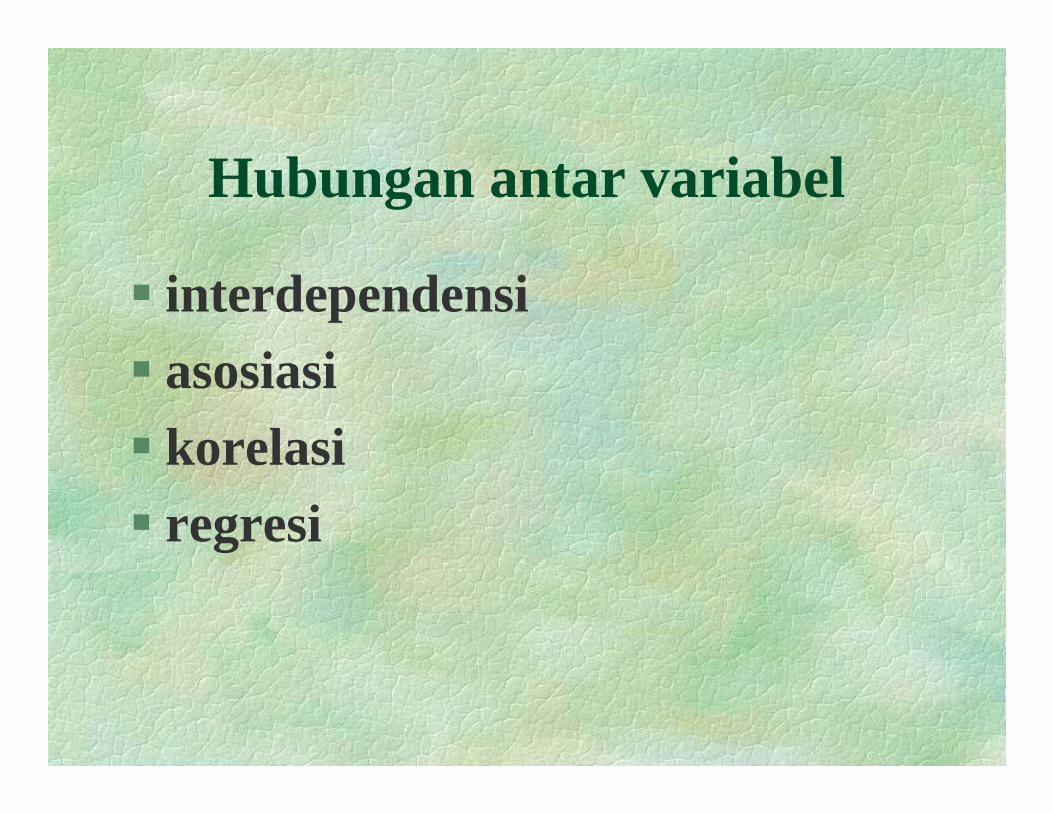
Hubungan antar variabel
interdependensi i iasosiasi
korelasikorelasiregresi
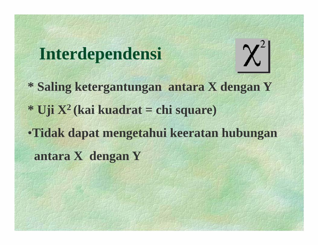
Interdependensi
* Saling ketergantungan antara X dengan Y
* Uji X2 (k i k d t hi )* Uji X2 (kai kuadrat = chi square)
•Tidak dapat mengetahui keeratan hubungan p g g
antara X dengan Y

Asosiasi* Kelanjutan dari uji interdependensi
* ji K fi i k ti i* uji : Koefisien kontingensi
Phi
Cramer’s V
* il i t 0 1 (t k d b i i )* nilai antara 0 - 1 (tak ada - berasosiasi sempurna)
* tidak menunjukkan arah hubungan (pos / neg)

Korelasi* menunjukkan arah hubungan
* Uji :
r product moment Pearsonr product moment Pearson
Spearman
Kendall
* Nilai : -1 s/d +1
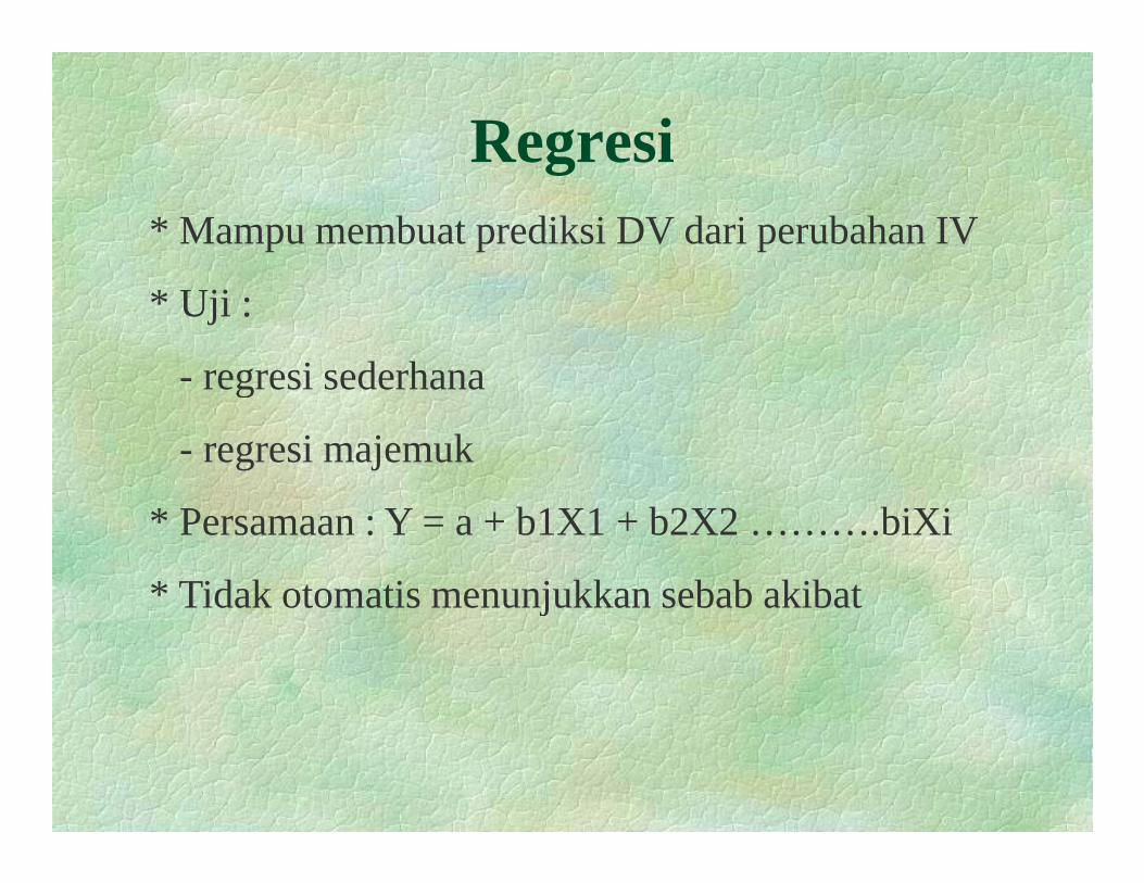
Regresig* Mampu membuat prediksi DV dari perubahan IV
* Uji :
- regresi sederhanaregresi sederhana
- regresi majemuk
* Persamaan : Y = a + b1X1 + b2X2 ……….biXi
* Tidak otomatis menunjukkan sebab akibatj

Chi squared (X2) testChi-squared (X2) testUsed to test whether there is an interdependence pbetween the row variable and the column variable.
Observed number
influenza vaccine placebo totalY 20 80 100
Observed number
Yes 20 80 100
No 220 140 360
Total 240 220 460
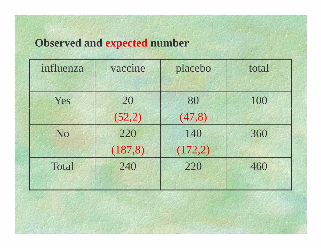
Observed and expected numberObserved and expected number
influenza vaccine placebo total
Yes 20 80 100(52,2) (47,8)
No 220 140 360(187,8) (172,2)
Total 240 220 460

Formula
X2 = (O – E)2
EE
The greater the difference between the observed andThe greater the difference between the observed and expected numbers, the larger the value of X2 and the less likely it is that the difference is due to chance

Continuity correctionY t ’ ti it ti= Yate’s continuity correction
Is always advisable although it has most effect when the expected numbers are smallpWhen they are very small the alternative is
Fi h ’ t t tFischer’s exact test
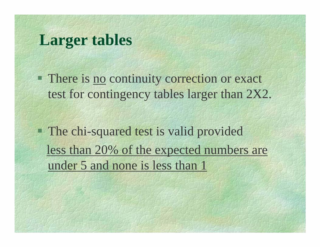
Larger tablesg
There is no continuity correction or exactThere is no continuity correction or exact test for contingency tables larger than 2X2.
The chi-squared test is valid provided less than 20% of the expected numbers are under 5 and none is less than 1
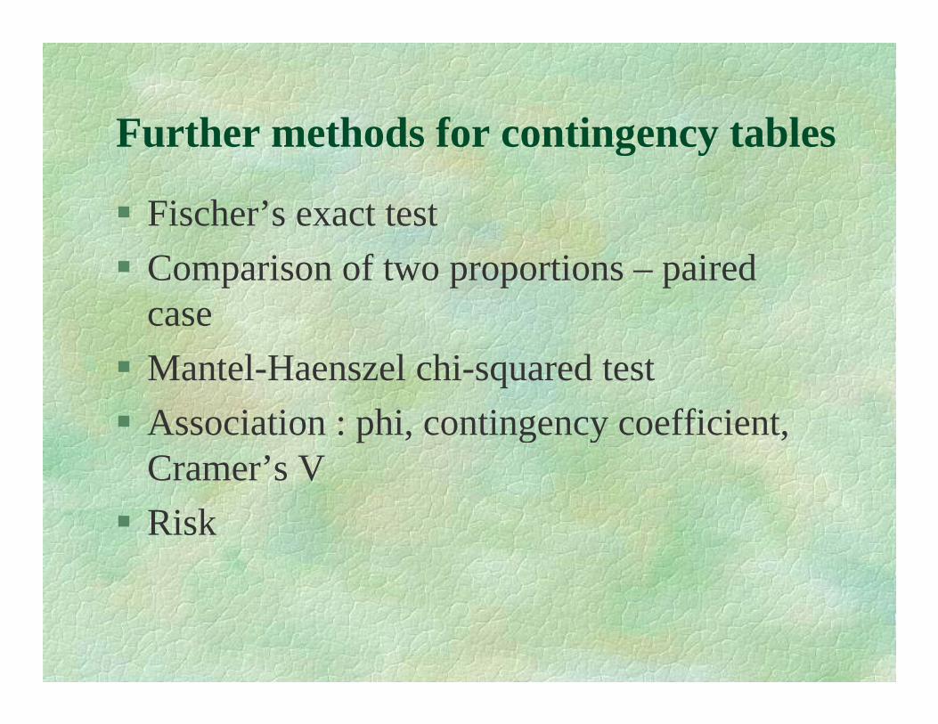
Further methods for contingency tablesFurther methods for contingency tables
Fischer’s exact testFischer s exact testComparison of two proportions – paired casecaseMantel-Haenszel chi-squared testAssociation : phi, contingency coefficient, Cramer’s VRisk
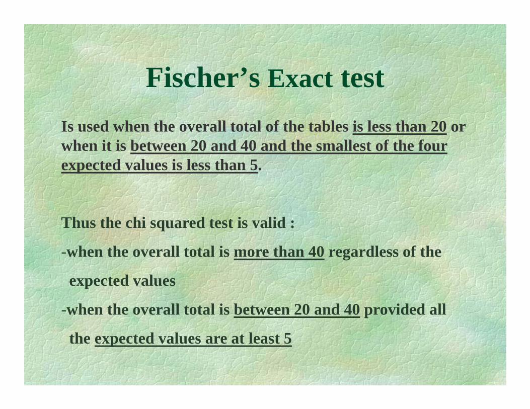
Fischer’s Exact testIs used when the overall total of the tables is less than 20 or
Fischer’s Exact testIs used when the overall total of the tables is less than 20 or when it is between 20 and 40 and the smallest of the four expected values is less than 5.
Thus the chi squared test is valid :q
-when the overall total is more than 40 regardless of the
expected valuesexpected values
-when the overall total is between 20 and 40 provided all
th t d l t l t 5the expected values are at least 5
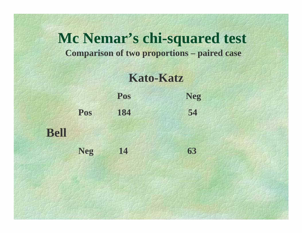
Mc Nemar’s chi-squared testc Ne a s c squa ed testComparison of two proportions – paired case
Kato-KatzPos Neg
Pos 184 54
BellBellNeg 14 63
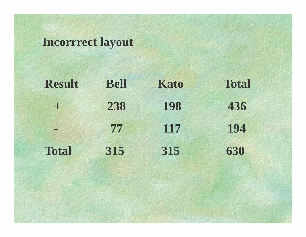
Incorrrect layoutIncorrrect layout
Result Bell Kato Total
+ 238 198 436+ 238 198 436
- 77 117 194
Total 315 315 630
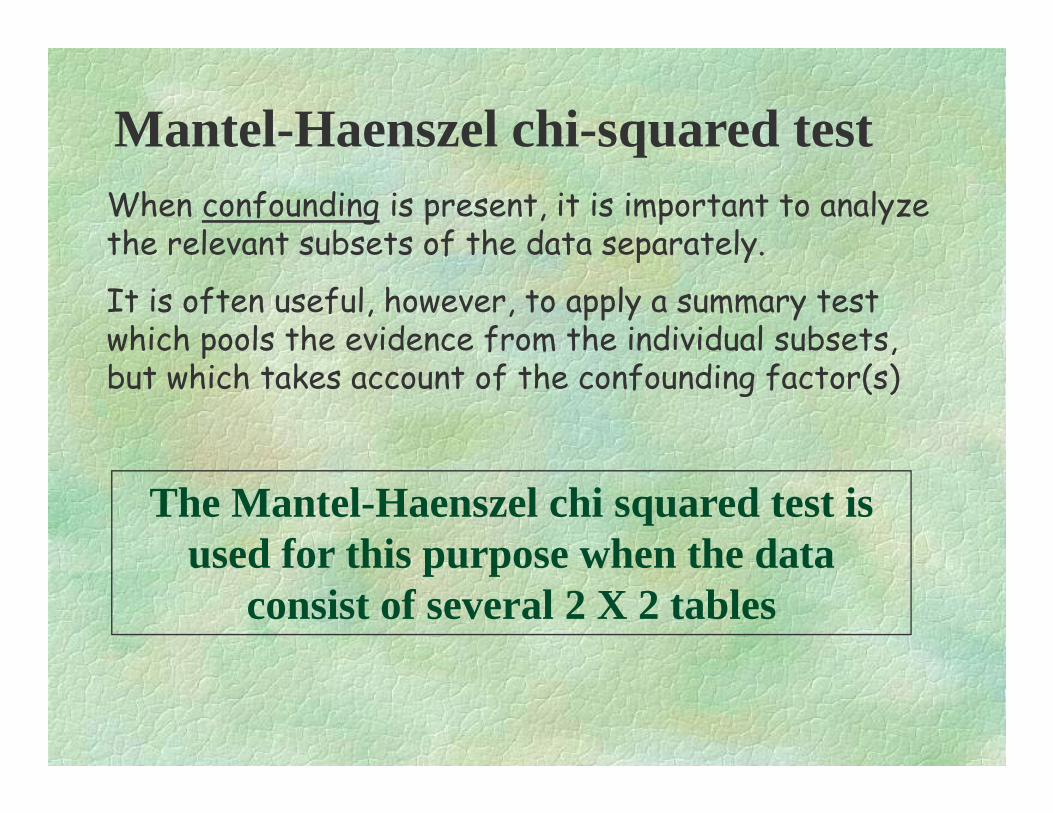
Mantel-Haenszel chi-squared testqWhen confounding is present, it is important to analyze the relevant subsets of the data separately. the relevant subsets of the data separately.
It is often useful, however, to apply a summary test which pools the evidence from the individual subsets, pbut which takes account of the confounding factor(s)
The Mantel-Haenszel chi squared test is used for this purpose when the dataused for this purpose when the data
consist of several 2 X 2 tables
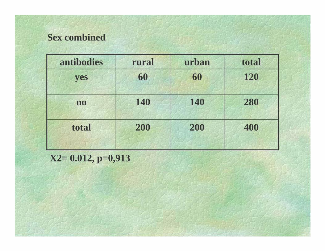
Sex combined
antibodies rural urban totalyes 60 60 120yes 60 60 120
no 140 140 280
total 200 200 400
X2= 0.012, p=0,913
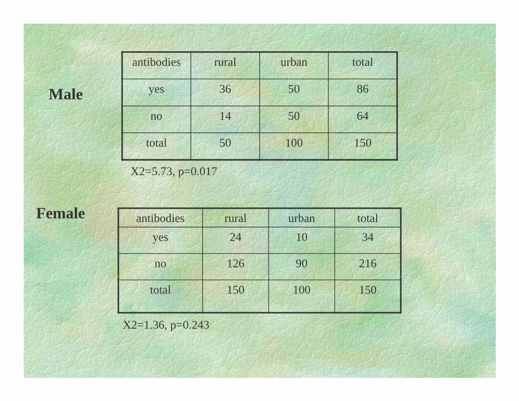
antibodies rural urban total
yes 36 50 86
no 14 50 64
Male
total 50 100 150
X2=5.73, p=0.017
antibodies rural urban totalFemale
, p
yes 24 10 34
no 126 90 216
total 150 100 150
X2=1 36 p=0 243X2 1.36, p 0.243
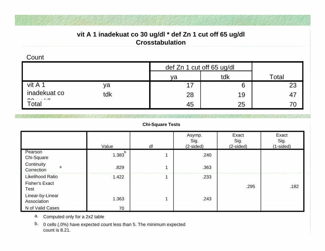
Crosstabsvit A 1 inadekuat co 30 ug/dl * def Zn 1 cut off 65 ug/dlCrosstabulation
Count
ya tdkdef Zn 1 cut off 65 ug/dl
Total17 6 2328 19 4745 25 70
yatdk
vit A 1inadekuat co30 ug/dlTotal
ya tdk Total
Asymp.Sig
ExactSig
ExactSig
Chi-Square Tests
1.383b
1 .240
.829 1 .363
PearsonChi-SquareContinuityCorrection
a
Value dfSig.
(2-sided)Sig.
(2-sided)Sig.
(1-sided)
1.422 1 .233
.295 .182
1.363 1 .243
Likelihood RatioFisher's ExactTestLinear-by-LinearAssociation
70N of Valid Cases
Computed only for a 2x2 tablea.
0 cells (.0%) have expected count less than 5. The minimum expectedcount is 8.21.
b.

Crosstabs
vit A 1 inadekuat co 30 ug/dl * def Zn 1 cut off 65 ug/dl Crosstabulation
ya tdkdef Zn 1 cut off 65 ug/dl
Total
g g
17 6 23
14.8 8.2 23.0
CountExpectedCount
yavit A 1inadekuat co30 ug/dl
28 19 47
30.2 16.8 47.0
CountExpectedCount
tdk
45 25 70
45.0 25.0 70.0
CountExpectedCount
Total
Count

Asymp.Sig
ExactSig
ExactSig
Chi-Square Tests
1.383b
1 .240
829 1 363
PearsonChi-SquareContinuity a
Value dfSig.
(2-sided)Sig.
(2-sided)Sig.
(1-sided)
.829 1 .363
1.422 1 .233
.295 .182
Correctiona
Likelihood RatioFisher's ExactTest
1.363 1 .243
70
Linear-by-LinearAssociationN of Valid Cases
Computed only for a 2x2 tablea. p y
0 cells (.0%) have expected count less than 5. The minimum expectedcount is 8.21.
b.
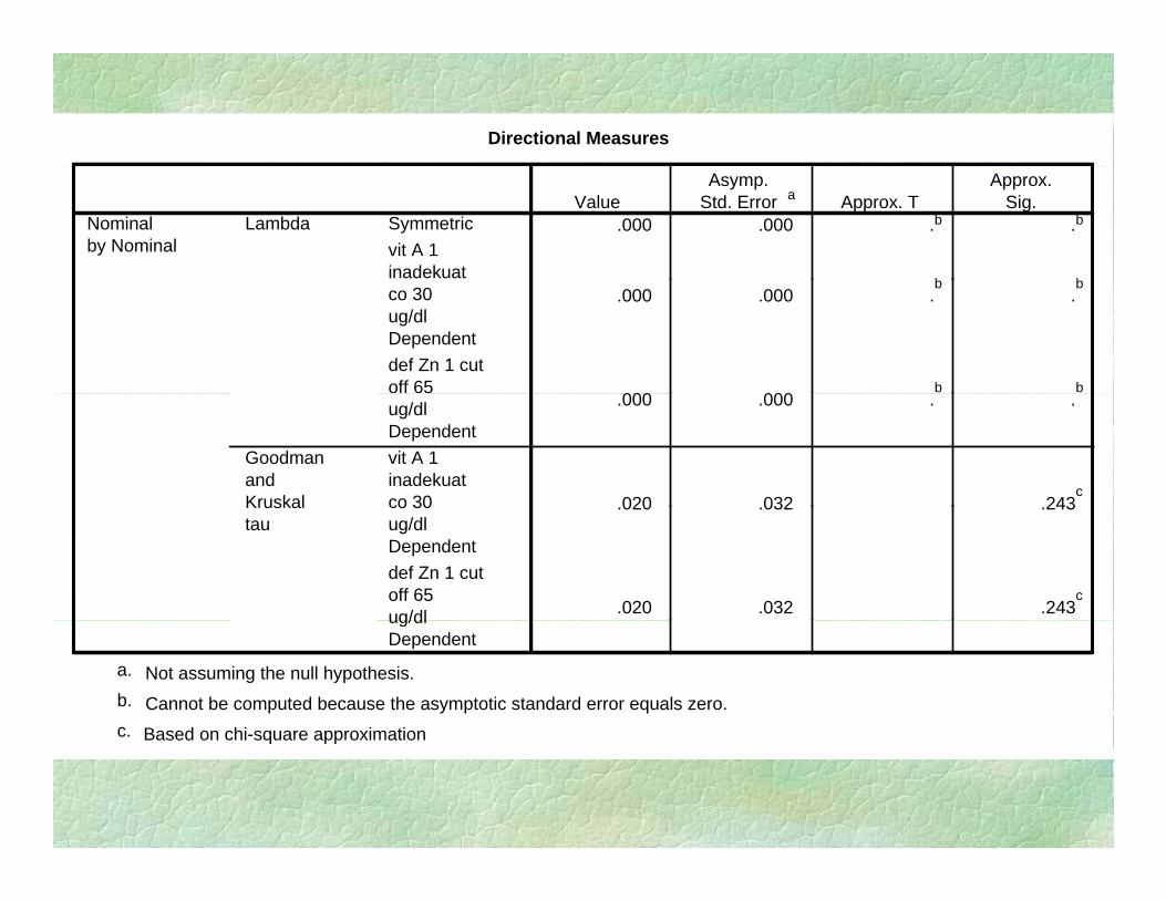
Directional Measures
.000 .000 .b .b
b b
Symmetricvit A 1inadekuat
LambdaNominalby Nominal
ValueAsymp.
Std. Error a Approx. TApprox.
Sig.
.000 .000 .b
.b
000 000b b
co 30ug/dlDependentdef Zn 1 cutoff 65
.000 .000 . .
020 032 243c
ug/dlDependentvit A 1inadekuatco 30
GoodmanandKruskal .020 .032 .243
.020 .032 .243c
co 30ug/dlDependentdef Zn 1 cutoff 65ug/dl
Kruskaltau
ug/dlDependent
Not assuming the null hypothesis.a.
Cannot be computed because the asymptotic standard error equals zero.b.
Based on chi square approximationc Based on chi-square approximationc.
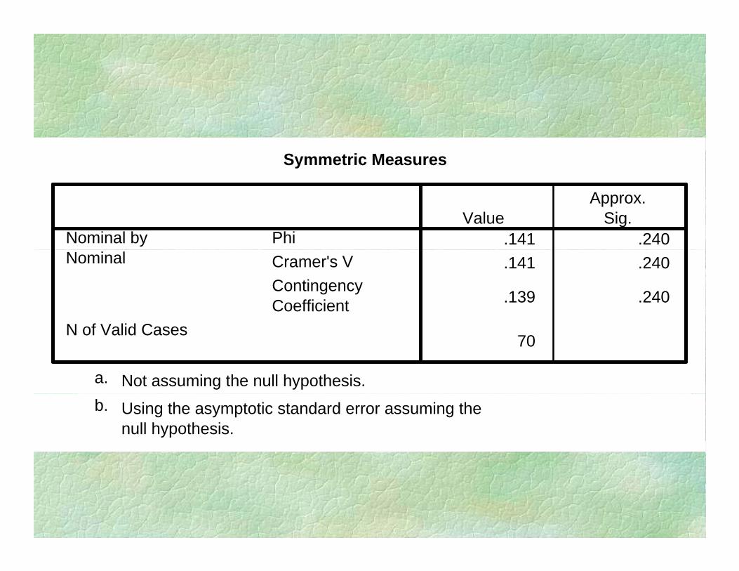
Symmetric Measures
.141 .240PhiNominal byValue
Approx.Sig.
.141 .240
.139 .240
Cramer's VContingencyCoefficient
Nominal
70N of Valid Cases
Not assuming the null hypothesis.a.
Using the asymptotic standard error assuming thenull hypothesis.
b.
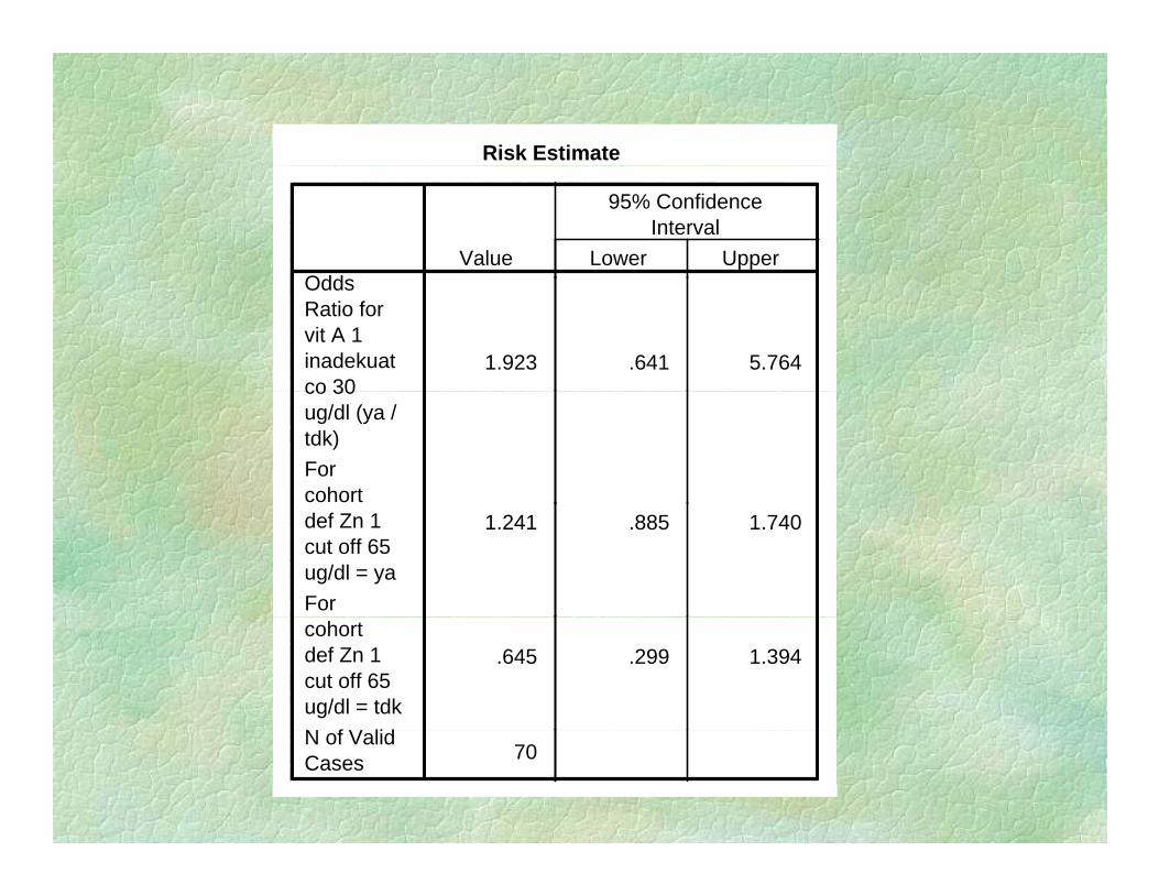
Risk Estimate
OddValue Lower Upper
95% ConfidenceInterval
1.923 .641 5.764
OddsRatio forvit A 1inadekuatco 30co 30ug/dl (ya /tdk)Forcohort
1.241 .885 1.740def Zn 1cut off 65ug/dl = yaFor
.645 .299 1.394cohortdef Zn 1cut off 65ug/dl = tdkN f V lid
70N of ValidCases