Hitung Sample Size
42
Sampling and Sample Size Calculation Authors Nick Fox Amanda Hunn Nigel Mathers This Resource Pack is one of a series produced by The NIHR RDS for the East Midl ands / The NIHR RDS for Yorkshire and the Humber. This series has been funded by The NIHR RDS EM / YH. The NIHR Research Design Service for Yorkshire & the Humber
Transcript of Hitung Sample Size
8/21/2019 Hitung Sample Size
http://slidepdf.com/reader/full/hitung-sample-size 1/41
Sampling and SampleSize Calculation
Authors
Nick Fox
Amanda Hunn
Nigel Mathers
This Resource Pack is one of a series produced by The NIHR RDS for the EastMidlands / The NIHR RDS for Yorkshire and the Humber. This series has beenfunded by The NIHR RDS EM / YH.
The NIHR Research Design Servicefor Yorkshire & the Humber
8/21/2019 Hitung Sample Size
http://slidepdf.com/reader/full/hitung-sample-size 2/41
The NIHR RDS for the East Midlands / Yorkshire & the Humber 2009 2 Sampling
This Resource Pack may be freely photocopied and distributed for the benefit ofresearchers. However it is the copyright of The NIHR RDS EM / YH and theauthors and as such, no part of the content may be altered without the priorpermission in writing, of the Copyright owner.
Reference as:Fox N., Hunn A., and Mathers N. Sampling and sample size calculationThe NIHR RDS for the East Midlands / Yorkshire & the Humber 2007.
Nick Fox School of Health and Related Research(ScHARR)University of SheffieldRegent Court30 Regent StreetSheffieldS1 4DA
Amanda Hunn Tribal Consulting, Tribal House,7 Lakeside, Calder Island WayWakefield
WF2 7AW
Nigel Mathers Academic Unit of Primary MedicalCare,Community Sciences Centre,University of Sheffield,Northern General Hospital,Herries Road,Sheffield S5 7AUUnited Kingdom
Last updated: May 2009
The NIHR RDS for the EastMidlandsDivision of Primary Care,14
th Floor, Tower building
University of NottinghamUniversity ParkNottinghamNG7 2RDTel: 0115 823 0500
www.rds-eastmidlands.nihr.ac.uk
Leicester: [email protected]
Nottingham: [email protected]
The NIHR RDS for Yorkshire & the Humber
ScHARRThe University of SheffieldRegent Court30 Regent Street SheffieldS1 4DATel: 0114 222 0828
www.rds-yh.nihr.ac.uk
Sheffield: [email protected] Leeds: [email protected] York: [email protected]
© Copyright of The NIHR RDS EM / YH
(2009)
8/21/2019 Hitung Sample Size
http://slidepdf.com/reader/full/hitung-sample-size 3/41
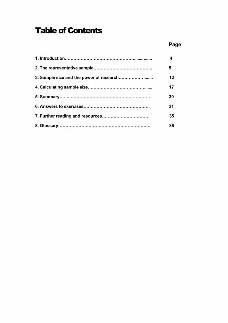
Table of Contents
Page
1. Introduction…………………………………………............... 4
2. The representative sample………………………………….. 5
3. Sample size and the power of research………………....... 12
4. Calculating sample size…………………………………....... 17
5. Summary……………………………………………………… 30
6. Answers to exercises………………………………………. 31
7. Further reading and resources…………………………… 35
8. Glossary………………………………………………………. 36
8/21/2019 Hitung Sample Size
http://slidepdf.com/reader/full/hitung-sample-size 4/41
The NIHR RDS for the East Midlands / Yorkshire & the Humber 2009 4 Sampling
1. Introduction
Sampling and sample size are crucial issues in pieces of quantitative research,which seek to make statistically based generalisations from the study results to
the wider world. To generalise in this way, it is essential that both the samplingmethod used and the sample size are appropriate, such that the results arerepresentative, and that the statistics can discern associations or differenceswithin the results of a study.
LEARNING OBJECTIVESHaving successfully completed this pack, you will be able to:
• distinguish between random and non-random methods of sample selection
• describe the advantages of random sample selection
• identify the different methods of random sample selection• match the appropriate methods of sample selection to the research question and
design
• realise the importance of estimating the optimal sample size, when designing anew study, and of seeking independent advice at this stage
• describe the factors influencing sample size
• make a preliminary estimate of the appropriate sample size.
Working through this pack
The study time involved in this pack is approximately 10 hours. In addition to the
written text, the pack includes exercises for completion. We suggest that as youwork through the pack, you establish for yourself a ‘reflective log’, linking the workin the pack to your own research interests and needs, and documenting yourreflections on the ethnographic method. Include your responses to the exercisesplus your own thoughts as you read and consider the material.
At all stages of your work, you may find the Glossary contained at the end of thisresource pack to be of assistance.
8/21/2019 Hitung Sample Size
http://slidepdf.com/reader/full/hitung-sample-size 5/41
The NIHR RDS for the East Midlands / Yorkshire & the Humber 2009 5 Sampling
2. The representative sample
It is an explicit or implicit objective of most studies in health care which ‘count’something or other (quantitative studies), to offer conclusions that aregeneralisable.
This means that the findings of a study apply to situations otherthan that of the cases in the study. To give a hypothetical example, Smith andJones’ (1997) study of consultation rates in primary care which was based ondata from five practices in differing geographic settings (urban, suburban, rural)finds higher rates in the urban environment. When they wrote it up for publication,Smith and Jones used statistics to claim their findings could be generalised: thedifferences applied not just to these five practices, but to all practices in thecountry.
For such a claim to be legitimate (technically, for the study to possess ‘externalvalidity’), the authors must persuade us that their sample was not biased: that itwas representative. Although other criteria must also be met (for instance, that
the design was both appropriate and carried out correctly - the study’s ‘internalvalidity’ and ‘reliability’), it is the representativeness of a sample which allows theresearcher to generalise the findings to the wider population. If a study has anunrepresentative or biased sample, then it may still have internal validity andreliability, but it will not be generalisable (will not possess external validity).Consequently the results of the study will be applicable only to the group understudy.
It is essential to a study’s design (assuming that study wants to generalise and isnot simply descriptive of one setting) that sampling is taken seriously. The firstpart of this pack looks at how to gather a ‘representative’ sample which gives a
study external validity and permits valid generalisation.
However, there is a second issue which must be addressed in relation tosampling, and this is predominantly a question of sample size. Generalisationsfrom data to wider population depend upon a kind of statistic which testsinferences or hypotheses . For instance, the t-test can be used to test ahypothesis that there is a difference between two populations, based on a samplefrom each. To give an example, we select 100 males and 100 females and testtheir body mass index. We find a difference in our samples, and wish to arguethat the difference found is not an accident (due to chance), but reflects an actualdifference in the wider populations from which the samples were drawn. We use
a t-test to see if we can make this claim legitimately.
Most people know that the larger a sample size, the more likely it is that a findingof a difference such as this is not due to chance, but really does mean there is adifference between men and women. Many quantitative studies undertaken and published in medical journals do not have a sufficient sample size to adequatelytest the hypothesis which the study was designed to explore. Such studies are,by themselves, of little use, and -- for example in the case of drug trials -- couldbe dangerous if their findings were generalised.We will consider these issues of sample size, and how to calculate an adequatesize for a study sample in the second half of this pack. Before that, let us think in
greater detail about what a sample is.
8/21/2019 Hitung Sample Size
http://slidepdf.com/reader/full/hitung-sample-size 6/41
The NIHR RDS for the East Midlands / Yorkshire & the Humber 2009 6 Sampling
2.1 Why do we need to select a sample anyway?In some circumstances it is not necessary to select a sample. If the subjects ofyour study are very rare, for instance a disease occurring only once in 100 000children, then you might decide to study every case you can find. More usually,however, you are likely to find yourself in a situation where the potential subjects
of your study are much more common and you cannot practically includeeverybody. For example, a study of everybody in the UK who had beendiagnosed as suffering from asthma would be impossible: it would take too longand cost too much money.
So it is necessary to find some way of reducing the number of subjects includedin the study without biasing the findings in any way. Random sampling is one wayof achieving this, and with appropriate statistics such a study can yieldgeneralisable findings at far lower cost. Samples can also be taken using non-random techniques, but in this pack we will emphasise random sampling, which --if conducted adequately -- will ensure external validity.
2.2 Random SamplingTo obtain a random (or probability) sample, the first step is to define the targetpopulation from which it is to be drawn. This population is known as the samplingframe, and can be thought of as a list of all the people / patients relevant to thestudy. For instance, you are interested in doing a study of children aged betweentwo and ten years diagnosed within the last month as having otitis media. Or youwant to study adults (aged 16-65 years) diagnosed as having asthma andreceiving drug treatment for asthma in the last six months, and living in a definedgeographical region. In each case, these limits define the sampling frame. If theresearch design is based on an experimental design, such as a randomisedcontrolled trial (RCT), with two or more groups, then the population frame mayoften be very tightly defined with strict eligibility criteria.
Within an RCT, potential subjects are randomly allocated to either theintervention (treatment) group or the control group. By randomly allocatingsubjects to each of the groups, potential differences between the comparisongroups should be much reduced. In this way confounding variables (i.e. variablesyou haven't thought of, or controlled for) will be more equally distributed betweeneach of the groups and will be less likely to influence the outcome (or dependent
variable) in either of the groups.
Randomisation within an experimental design is a way of ensuring control overconfounding variables and as such it allows the researcher to have greaterconfidence in identifying real associations between an independent variable (apotential cause or predictor) and a dependent variable (the effect or outcomemeasure).
The term random may imply to you that it is possible to take some sort ofhaphazard or ad hoc approach, for example stopping the first 20 people you meetin the street for inclusion in your study. This is not random in the true sense of the
word. To be a 'random' sample, every individual in the population must have an
8/21/2019 Hitung Sample Size
http://slidepdf.com/reader/full/hitung-sample-size 7/41
The NIHR RDS for the East Midlands / Yorkshire & the Humber 2009 7 Sampling
equal probability of being selected. In order to carry out random samplingproperly, strict procedures need to be adhered to.
Random sampling techniques can be split into simple random sampling andsystematic sampling.
2.3 Simple Random SamplingIf selections are made purely by chance this is known as simple random sampling.So, for instance, if we had a population containing 5000 people, we could allocateevery individual a different number. If we wanted to achieve a sample size of 200,we could achieve this by pulling 200 of the 5000 numbers out of a hat. This wouldbe an example of simple random sampling - sometimes also called IndependentRandom Sampling because, as the probability of a person being selected isindependent of the identity of the other people selected.
The usual method of obtaining random numbers is to use computer packagessuch as SPSS. Tables of random numbers may also be found in the appendicesof most statistical textbooks.
Simple random sampling, although technically valid, is a very laborious way ofcarrying out sampling. A simpler and quicker way is to use systematic sampling.
2.4 Systematic SamplingSystematic sampling is a more commonly employed method. After numbers areallocated to everybody in the population frame, the first individual is picked usinga random number table and then subsequent subjects are selected using a fixedsampling interval, i.e. every nth person.
Assume, for example, that we wanted to carry out a survey of patients withasthma attending clinics in one city. There may be too many to intervieweveryone, so we want to select a representative sample. If there are 3,000 peopleattending the clinics in total and we only require a sample of 200, we would needto:
• calculate the sampling interval by dividing 3,000 by 200 to give a samplingfraction of 15
• select a random number between one and 15 using a set of random tables
• if this number were 13, we select the individual allocated number 13 and thengo on to select every 15th person, i.e. numbers 28, then 43, then 58, and so on.
This will give us a total sample size of 200 as required.
Care needs to be taken when using a systematic sampling method in case there issome bias in the way that lists of individuals are compiled. For example, if all thehusbands' names precede wives' names and the sampling interval is an evennumber, then we could end up selecting all women and no men.
8/21/2019 Hitung Sample Size
http://slidepdf.com/reader/full/hitung-sample-size 8/41
The NIHR RDS for the East Midlands / Yorkshire & the Humber 2009 8 Sampling
2.5 Stratified Random SamplingStratified sampling is a way of ensuring that particular strata or categories ofindividuals are represented in the sampling process.
If, for example, we want to study consultation rates in a general practice, and we
know that approximately four per cent of our population frame is made up of a particular ethnic minority group, there is a chance that with simple randomsampling or systematic sampling we could end up with no ethnic minorities (or amuch reduced proportion) in our sample. If we wanted to ensurethat our sample was representative of the population frame, then we wouldemploy a stratified sampling method.
• First we would split the population into the different strata, in this case,separating out those individuals with the relevant ethnic background.
• We would then apply random sampling techniques to each of the two ethnicgroups separately, using the same sampling interval in each group.
• This would ensure that the final sampling frame was representative of theminority group we wanted to include, on a pro-rata basis with the actualpopulation.
2.6 Disproportionate SamplingIf our objective were to compare the results of our minority group with the largergroup, then we would have difficulty in doing so, using the proportionate stratifiedsampling just described. This is because the numbers achieved in the minority
group, although pro-rata those of the population, may not be large enough to givea reasonable chance of demonstrating statistical differences (if such differencesdo in fact exist).
To compare the survey results of the minority individuals with those of the largergroup, it is necessary to use a disproportion sampling method. Withdisproportionate sampling, the strata selected are not selected pro-rata to theirsize in the wider population. For instance, if we are interested in comparing thereferral rates for particular minority groups with other larger groups, then it isnecessary to over sample the smaller categories in order to achieve statisticalpower, that is, in order to be able to demonstrate statistically significantdifferences between groups if such differences exist.
(Note that, if subsequently we wish to refer to the total sample as a whole,representative of the wider population, then it will become necessary to re-weightthe categories back into the proportions in which they are represented in reality.For example, if we wanted to compare the views and satisfaction levels of womenwho gave birth at home compared with the majority of women who have givenbirth in hospital, a systematic or random sample, although representative of allwomen giving birth would not produce a sufficient number of women giving birthat home to be able to compare the results, unless the total sample was so bigthat it would take many years to collate. We would also end up interviewing morewomen than we needed who have given birth in hospital. In this case it would be
necessary to over-sample or over-represent those women giving birth at home tohave enough individuals in each group in order to compare them. We would
8/21/2019 Hitung Sample Size
http://slidepdf.com/reader/full/hitung-sample-size 9/41
The NIHR RDS for the East Midlands / Yorkshire & the Humber 2009 9 Sampling
therefore use disproportionate stratified random sampling to select the sample inthis instance.)
The important thing to note here about disproportionate sampling is that samplingis still taking place within each stratum or category. So we would use systematic
or simple random selection to select a sample from the ‘majority’ group and thesame process to select samples from the minority groups.
2.7 Cluster (Multistage) SamplingCluster sampling is a method frequently employed in national surveys where it isuneconomic to carry out interviews with individuals scattered across the country.Cluster sampling allows individuals to be selected in geographic batches. Forinstance, before selecting individual people at random, the researcher maydecide to focus on certain ‘areas’, e.g. towns, electoral wards or general practices
- selecting these by a method of random sampling. Once this was done, theycould either i) select all the individuals within these areas, or ii) use randomsampling to select just a proportion of the individuals within these chosen areas.
Although cluster sampling is a very valuable technique and is widely used, it isworth noting that it does not produce strictly independent samples, since theknowledge that one person in a specific cluster has been selected will increasethe probability that others in the same cluster will also be selected.Obviously care must be taken to ensure that the cluster units selected aregenerally representative of the population and are not strongly biased in any way.If, for example, all the general practices selected for a study were single-handed,
this would not be representative of all general practices.
2.8 Non-Random SamplingNon-random (or non-probability) sampling is not used very often in quantitativemedical social research surveys, but it is used increasingly in market researchand commissioned studies. The technique most commonly used is known asquota sampling.
Quota Sampling
Quota sampling is a technique for sampling whereby the researcher decides in
advance on certain key characteristics which s/he will use to stratify the sample.Interviewers are often set sample quotas in terms of age and sex. For example,consider a market research study where interviewers will stop people in the streetto ask them a series of questions on consumer preferences. The interviewermight be asked to sample 200 people, of whom 100 should be male and 100should be female - and, within each of these groups, there should be 25 people ineach of the age-groups: under-20, 20-39, 40-59 and over-60. The differencewith a stratified sample is that the respondents in a quota sample are notrandomly selected within the strata. The respondents may be selected justbecause they are accessible to the interviewer. Because random sampling is notemployed, it is not possible to
apply inferential statistics and generalise the findings to a wider population.
8/21/2019 Hitung Sample Size
http://slidepdf.com/reader/full/hitung-sample-size 10/41
The NIHR RDS for the East Midlands / Yorkshire & the Humber 2009 10 Sampling
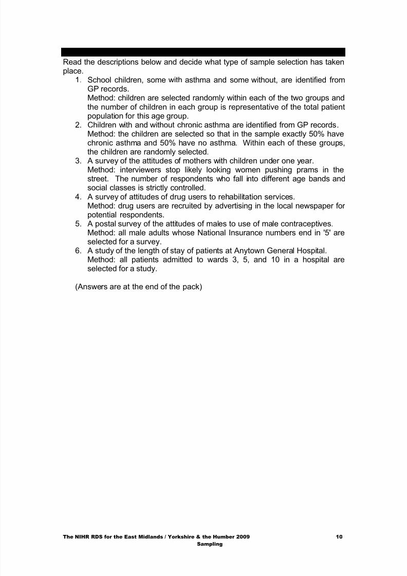
EXERCISE 1Read the descriptions below and decide what type of sample selection has takenplace.
1. School children, some with asthma and some without, are identified fromGP records.
Method: children are selected randomly within each of the two groups andthe number of children in each group is representative of the total patientpopulation for this age group.
2. Children with and without chronic asthma are identified from GP records.Method: the children are selected so that in the sample exactly 50% havechronic asthma and 50% have no asthma. Within each of these groups,the children are randomly selected.
3. A survey of the attitudes of mothers with children under one year.Method: interviewers stop likely looking women pushing prams in thestreet. The number of respondents who fall into different age bands andsocial classes is strictly controlled.
4. A survey of attitudes of drug users to rehabilitation services.Method: drug users are recruited by advertising in the local newspaper forpotential respondents.
5. A postal survey of the attitudes of males to use of male contraceptives.Method: all male adults whose National Insurance numbers end in '5' areselected for a survey.
6. A study of the length of stay of patients at Anytown General Hospital.Method: all patients admitted to wards 3, 5, and 10 in a hospital areselected for a study.
(Answers are at the end of the pack)
8/21/2019 Hitung Sample Size
http://slidepdf.com/reader/full/hitung-sample-size 11/41
The NIHR RDS for the East Midlands / Yorkshire & the Humber 2009 11 Sampling
2.9 Sampling in Qualitative ResearchSince the objective of qualitative research is to understand and give meaning to a socialprocess, rather than quantify and generalise to a wider population, it is inappropriate to
use random sampling or apply statistical tests. Sample sizes used in qualitative researchare usually very small and the application of statistical tests would be neither appropriatenor feasible.For details on this topic, please refer to the The NIHR RDS EM / YH resource pack“Qualitative Research” by Kate Windridge and Elizabeth Ockleford, 2007.
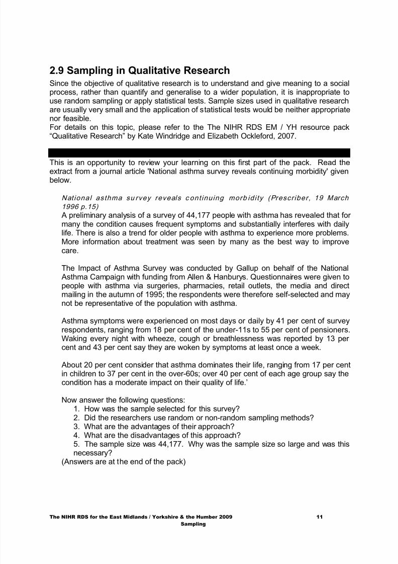
EXERCISE 2This is an opportunity to review your learning on this first part of the pack. Read theextract from a journal article 'National asthma survey reveals continuing morbidity' givenbelow.
Nat ional asthma su rvey reveals c ont inuing morb id i ty (Prescr iber, 19 March1996 p.15)
A preliminary analysis of a survey of 44,177 people with asthma has revealed that formany the condition causes frequent symptoms and substantially interferes with dailylife. There is also a trend for older people with asthma to experience more problems.More information about treatment was seen by many as the best way to improvecare.
The Impact of Asthma Survey was conducted by Gallup on behalf of the National Asthma Campaign with funding from Allen & Hanburys. Questionnaires were given topeople with asthma via surgeries, pharmacies, retail outlets, the media and direct
mailing in the autumn of 1995; the respondents were therefore self-selected and maynot be representative of the population with asthma.
Asthma symptoms were experienced on most days or daily by 41 per cent of surveyrespondents, ranging from 18 per cent of the under-11s to 55 per cent of pensioners.Waking every night with wheeze, cough or breathlessness was reported by 13 percent and 43 per cent say they are woken by symptoms at least once a week.
About 20 per cent consider that asthma dominates their life, ranging from 17 per centin children to 37 per cent in the over-60s; over 40 per cent of each age group say thecondition has a moderate impact on their quality of life.’
Now answer the following questions:1. How was the sample selected for this survey?2. Did the researchers use random or non-random sampling methods?3. What are the advantages of their approach?4. What are the disadvantages of this approach?5. The sample size was 44,177. Why was the sample size so large and was thisnecessary?
(Answers are at the end of the pack)
8/21/2019 Hitung Sample Size
http://slidepdf.com/reader/full/hitung-sample-size 12/41
The NIHR RDS for the East Midlands / Yorkshire & the Humber 2009 12 Sampling
3. Sample size and the power of research
In the previous section, we looked at methods of sampling. Now we want to turn to
another aspect of sampling: how big a sample needs to be in quantitative research toenable a study to have sufficient ‘power’ to do the job of testing a hypothesis. While thisdiscussion will necessarily take us into the realm of statistics, we will keep the ‘number-crunching’ to a minimum: what is important is that you understand the concepts (andknow a friendly statistician!).
At first glance, many pieces of research seem to choose a sample size merely on thebasis of what 'looks' about right, or what similar studies have used in the past, orperhaps simply for reasons of convenience: ten seems a bit small, and one hundredwould be difficult to obtain, so 40 is a happy compromise! Unfortunately a lot ofpublished research uses precisely this kind of logic. In the following section, we want toshow you why using such reasoning could make your research worthless. Choosing thecorrect size of sample is not a matter of preference, it is a crucial element of theresearch process without which you may well be spending months trying to investigate aproblem with a tool which is either completely useless, or over expensive in terms oftime and other resources.
3.1 The truth is out there: Hypotheses and samples As we noted earlier, most (but not all) quantitative studies aim to test a hypothesis. Ahypothesis is a kind of truth claim about some aspect of the world: for instance, the
attitudes of patients or the prevalence of a disease in a population. Research sets out totry to prove this truth claim (or, more properly, to reject the null hypothesis - a truth claimphrased as a negative).
For example, let us think about the following hypothesis:
Levels of ill-health are affected by deprivation
and the related null hypothesis:
Levels of ill-health are not affected by deprivation
Let us imagine that we have this as our research hypothesis, and we are planningresearch to test it. We will undertake a trial, comparing groups of patients in a practicewho are living in different socio-economic environments, to assess the extent of ill-healthin these different groupings. Obviously the findings of a study -- while interesting inthemselves -- only have value if they can be generalised, to discover something aboutthe topic which can be applied in other practices. If we find an association, then we willwant to do something to reduce ill-health (by reducing deprivation). So our study has tohave external validity, that is, the capacity to be generalised beyond the subjects actuallyin the study.The measurement of such generalisability of a study is done by statistical tests ofinference. You may be familiar with some such tests: tests such as the chi-squared test ,
8/21/2019 Hitung Sample Size
http://slidepdf.com/reader/full/hitung-sample-size 13/41
The NIHR RDS for the East Midlands / Yorkshire & the Humber 2009 13 Sampling
the t-test , and tests of correlation. We will not look at these tests in any detail, but weneed to understand that the purpose of these and other tests of statistical inference is toassess the extent to which the findings of a study can be accepted as valid for thepopulation from which the study sample has been drawn. If the statistics we use suggest
that the findings are 'true', then we can be happy to conclude (within certain limits ofprobability), that the study's findings can be generalised, and we can act on them (toimprove nutrition among children under five years, for instance).
From common sense, we see that the larger the sample is, the easier it is to be satisfiedthat it is representative of the population from which it is drawn: but how large does itneed to be? This is the question that we need to answer, and to do so, we need to thinka little more about the possibilities that our findings may not reflect reality: that we havecommitted an error in our conclusions.
3.2 Type 1 and Type 2 errorsWhat any researcher wants is to be right! They want to discover that there is anassociation between two variables: say, asthma and traffic pollution, but only if such anassociation really exists. If there is no such association, then they want their study tosupport the null hypothesis that the two are not related. (While the former may be moreexciting, both are important findings).
What no researcher wants is to be wrong! No-one wants to find an association whichdoes not really exist, or - just as importantly - not find an association which does exist.Both such situations can arise in any piece of research. The first (finding an association
which is not really there) is called a Type I error . It is the error of falsely rejecting a truenull hypothesis.
(Think through this carefully. What we are talking about here could also be called a false positive. An example would be a study which rejects the null hypothesis that there is noassociation between ill-health and deprivation. The findings suggest such an association,but in reality, no such relationship exists.)
The second kind of error, called a Type 2 error (usually written as Type II), occurs whena study fails to find an association which really does exist. It is then a matter of wronglyaccepting a false null hypothesis . (This is a false negative: using the ill-health and
deprivation example again, we conduct a study and find no association, missing onewhich really does exist.)
Both types of error are serious. Both have consequences: imagine the money whichmight be spent on reducing traffic pollution, and all the time it does not really affectasthma (a Type I error). Or imagine allowing traffic pollution to continue, while it really isaffecting children's health (a Type II error). Good research will minimise the chances ofcommitting both Type I and Type II errors as far as possible, although they can never beruled out absolutely.
8/21/2019 Hitung Sample Size
http://slidepdf.com/reader/full/hitung-sample-size 14/41
The NIHR RDS for the East Midlands / Yorkshire & the Humber 2009 14 Sampling
3.3 Statistical Significance and Statistical Power
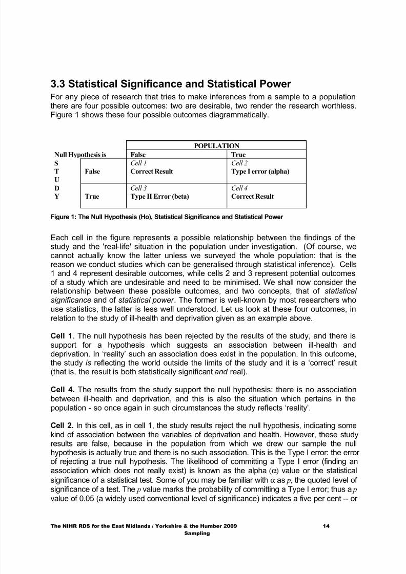
For any piece of research that tries to make inferences from a sample to a populationthere are four possible outcomes: two are desirable, two render the research worthless.Figure 1 shows these four possible outcomes diagrammatically.
POPULATION
Null Hypothesis is False True
S
T
U
False
Cell 1
Correct Result
Cell 2
Type I error (alpha)
D
Y True
Cell 3
Type II Error (beta)
Cell 4
Correct Result
Figure 1: The Null Hypothesis (Ho), Statistical Significance and Statistical Power
Each cell in the figure represents a possible relationship between the findings of thestudy and the 'real-life' situation in the population under investigation. (Of course, wecannot actually know the latter unless we surveyed the whole population: that is thereason we conduct studies which can be generalised through statistical inference). Cells1 and 4 represent desirable outcomes, while cells 2 and 3 represent potential outcomesof a study which are undesirable and need to be minimised. We shall now consider therelationship between these possible outcomes, and two concepts, that of statistical
significance and of statistical power . The former is well-known by most researchers whouse statistics, the latter is less well understood. Let us look at these four outcomes, inrelation to the study of ill-health and deprivation given as an example above.
Cell 1. The null hypothesis has been rejected by the results of the study, and there issupport for a hypothesis which suggests an association between ill-health anddeprivation. In ‘reality’ such an association does exist in the population. In this outcome,the study is reflecting the world outside the limits of the study and it is a ‘correct’ result(that is, the result is both statistically significant and real).
Cell 4. The results from the study support the null hypothesis: there is no association
between ill-health and deprivation, and this is also the situation which pertains in thepopulation - so once again in such circumstances the study reflects ‘reality’.
Cell 2. In this cell, as in cell 1, the study results reject the null hypothesis, indicating somekind of association between the variables of deprivation and health. However, these studyresults are false, because in the population from which we drew our sample the nullhypothesis is actually true and there is no such association. This is the Type I error: the errorof rejecting a true null hypothesis. The likelihood of committing a Type I error (finding anassociation which does not really exist) is known as the alpha (α) value or the statistical
significance of a statistical test. Some of you may be familiar with α as p, the quoted level ofsignificance of a test. The p value marks the probability of committing a Type I error; thus a p
value of 0.05 (a widely used conventional level of significance) indicates a five per cent -- or
8/21/2019 Hitung Sample Size
http://slidepdf.com/reader/full/hitung-sample-size 15/41
The NIHR RDS for the East Midlands / Yorkshire & the Humber 2009 15 Sampling
one in 20 -- chance of committing a Type I error . Cell 2 thus reflects an incorrect finding from
a study, and the α value represents the probability of this occurring.
Cell 3. This cell similarly reflects an undesirable outcome of a study. Here, as in Cell 4,
a study supports the null hypothesis, implying that there is no association between ill-health and deprivation in the population under investigation. But in reality, the nullhypothesis is false and there is an association in the real world which the study does notfind. This mistake is the Type II error of accepting a false null hypothesis . and is the
result of having a sample size which is too small to allow detection of the association bystatistical tests at an acceptable level of significance (say p = 0.05). The likelihood ofcommitting a Type II error is the beta (β) value of a statistical test, and the value (1 - β )is the statistical power of the test. Thus, the statistical power of a test is the likelihood ofavoiding a Type II error i.e. the probability that the test will reject the null hypothesiswhen the null hypothesis is false. Conventionally, a value of 0.80 or 80% is the targetvalue for statistical power, representing a likelihood that four times out of five a study will
reject a false null hypothesis, although values greater than 80% e.g. 90% are alsosometimes used. Outcomes of studies which fall into cell 3 are incorrect; β or its
complement (1-β) are the measures of the likelihood of such an outcome of a study.
All research should seek to avoid both Type I and Type II errors, which lead to incorrectinferences about the world beyond the study. In practice, there is a trade-off. Reducingthe likelihood of committing a Type I error by increasing the level of significance at whichone is willing to accept a positive finding reduces the statistical power of the test, thusincreasing the possibility of a Type II error (missing an association which exists).Conversely, if a researcher makes it a priority to avoid committing a Type II error, itbecomes more likely that a Type I error will occur (finding an association which does notexist). Now spend a few minutes doing this exercise to help you think about Type I andType II errors in research.
8/21/2019 Hitung Sample Size
http://slidepdf.com/reader/full/hitung-sample-size 16/41
The NIHR RDS for the East Midlands / Yorkshire & the Humber 2009 16 Sampling
EXERCISE 3
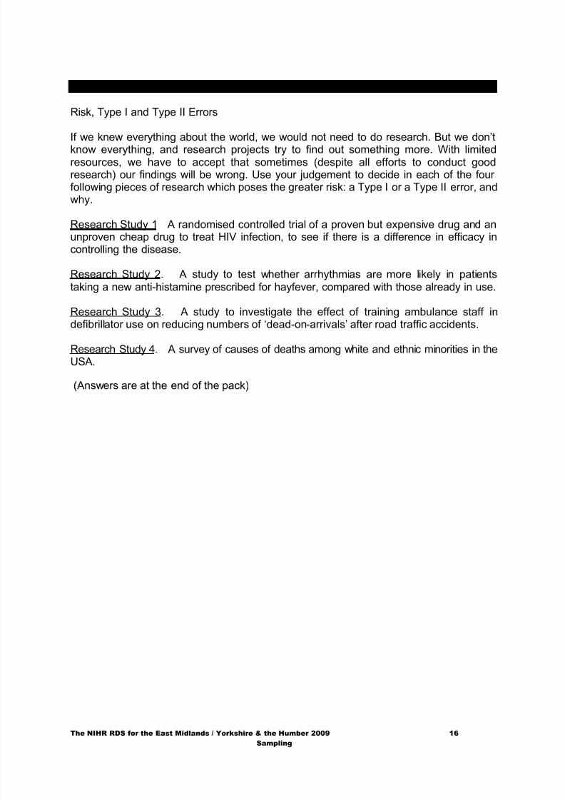
Risk, Type I and Type II Errors
If we knew everything about the world, we would not need to do research. But we don’tknow everything, and research projects try to find out something more. With limitedresources, we have to accept that sometimes (despite all efforts to conduct goodresearch) our findings will be wrong. Use your judgement to decide in each of the fourfollowing pieces of research which poses the greater risk: a Type I or a Type II error, andwhy.
Research Study 1 A randomised controlled trial of a proven but expensive drug and anunproven cheap drug to treat HIV infection, to see if there is a difference in efficacy incontrolling the disease.
Research Study 2. A study to test whether arrhythmias are more likely in patientstaking a new anti-histamine prescribed for hayfever, compared with those already in use.
Research Study 3. A study to investigate the effect of training ambulance staff indefibrillator use on reducing numbers of ‘dead-on-arrivals’ after road traffic accidents.
Research Study 4. A survey of causes of deaths among white and ethnic minorities in theUSA.
(Answers are at the end of the pack)
8/21/2019 Hitung Sample Size
http://slidepdf.com/reader/full/hitung-sample-size 17/41
The NIHR RDS for the East Midlands / Yorkshire & the Humber 2009 17 Sampling
4. Calculating sample size
In the rest of this pack, we will work through examples of the calculations needed to
determine an appropriate sample size. First, we will look at descriptive studies (which donot test a hypothesis). Then we will consider issues of statistical significance and powerin inferential, i.e. hypothesis-testing studies.
We will see that the formulae we need to use are relatively simple, and easy to calculateusing a pocket calculator or computer software - but the choice of the numbers to putinto the formulae is often not so straightforward, and the choices will often need to be justified, to the potential funding organisation and/or ethics committee who will assessingthe research proposal. We will also see that the consequences of getting these numberswrong, especially by under-estimating the required sample size - can be very seriousindeed - and have in the past often resulted in ‘hopeless’ studies being carried out,
which had no realistic chance of detecting the treatment effects or risk factors for whichthey were designed!
For these reasons, we strongly advise getting independent advice on sample size when youare designing your study - and this will usually be from either a trained statistician or from aresearcher in your field who has longstanding experience of study design. We hope that youwill be able to use the material in this resource pack for carrying out a preliminary samplesize calculation, and discussing these issues with the advisor.
4.1 Sample Size in Descriptive StudiesNot all quantitative studies involve hypothesis-testing, some studies merely seek todescribe the phenomena under examination. Whereas hypothesis testing will involvecomparing the characteristics of two or more groups, a descriptive survey may beconcerned solely with describing the characteristics of a single group. The aim of thistype of survey is often to obtain an accurate estimate of a particular figure, such as amean or a proportion. For example, we may want to know how many times, in anaverage week, that a general practitioner sees patients newly presenting with asthma. Inaddition we may also want to know what proportion of these patients admit to smokingfive or more cigarettes a day. In these circumstances, the aim is not to compare thisfigure with another group, but rather, to accurately reflect the real figure in the wider
population.
To calculate the required sample size in this situation, there are certain things that weneed to establish. We need to know:
1. The level of confidence we require concerning the true value of a mean or proportion.This is closely connected with the level of significance for statistical tests, such as a t-test.For example, we can be ‘95% confident’ that the true mean value lies somewhere within avalid 95% confidence interval, and this corresponds to significance testing at the 5% level(P < 0.05) of significance. Likewise, we can be ‘99% confident’ that the true mean value liessomewhere within a valid 99% confidence interval (which is a bit wider), and this
corresponds to significance testing at the 1% level (P < 0.01) of significance.
8/21/2019 Hitung Sample Size
http://slidepdf.com/reader/full/hitung-sample-size 18/41
The NIHR RDS for the East Midlands / Yorkshire & the Humber 2009 18 Sampling
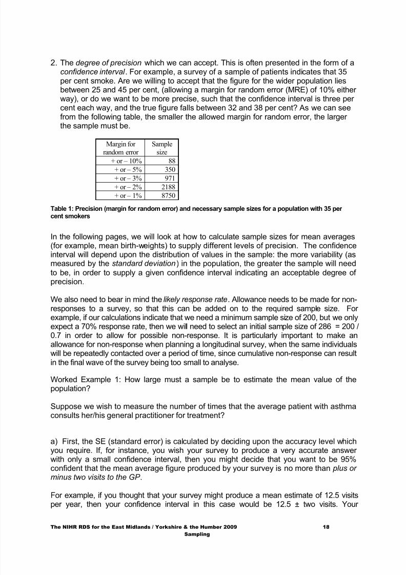
2. The degree of precision which we can accept. This is often presented in the form of aconfidence interval . For example, a survey of a sample of patients indicates that 35per cent smoke. Are we willing to accept that the figure for the wider population liesbetween 25 and 45 per cent, (allowing a margin for random error (MRE) of 10% either
way), or do we want to be more precise, such that the confidence interval is three percent each way, and the true figure falls between 32 and 38 per cent? As we can seefrom the following table, the smaller the allowed margin for random error, the largerthe sample must be.
Margin forrandom error
Samplesize
+ or – 10% 88
+ or – 5% 350
+ or – 3% 971
+ or – 2% 2188
+ or – 1% 8750
Table 1: Precision (margin for random error) and necessary sample sizes for a population with 35 percent smokers
In the following pages, we will look at how to calculate sample sizes for mean averages(for example, mean birth-weights) to supply different levels of precision. The confidenceinterval will depend upon the distribution of values in the sample: the more variability (asmeasured by the standard deviation) in the population, the greater the sample will needto be, in order to supply a given confidence interval indicating an acceptable degree ofprecision.
We also need to bear in mind the likely response rate. Allowance needs to be made for non-responses to a survey, so that this can be added on to the required sample size. Forexample, if our calculations indicate that we need a minimum sample size of 200, but we onlyexpect a 70% response rate, then we will need to select an initial sample size of 286 = 200 /0.7 in order to allow for possible non-response. It is particularly important to make anallowance for non-response when planning a longitudinal survey, when the same individualswill be repeatedly contacted over a period of time, since cumulative non-response can resultin the final wave of the survey being too small to analyse.
Worked Example 1: How large must a sample be to estimate the mean value of thepopulation?
Suppose we wish to measure the number of times that the average patient with asthmaconsults her/his general practitioner for treatment?
a) First, the SE (standard error) is calculated by deciding upon the accuracy level whichyou require. If, for instance, you wish your survey to produce a very accurate answerwith only a small confidence interval, then you might decide that you want to be 95%confident that the mean average figure produced by your survey is no more than plus orminus two visits to the GP .
For example, if you thought that your survey might produce a mean estimate of 12.5 visits
per year, then your confidence interval in this case would be 12.5 ± two visits. Your
8/21/2019 Hitung Sample Size
http://slidepdf.com/reader/full/hitung-sample-size 19/41
The NIHR RDS for the East Midlands / Yorkshire & the Humber 2009 19 Sampling
confidence interval would then tell you that you could reasonably (more detail on what‘reasonably’ means below!) expect the true average rate of visits in the population to besomewhere between 10.5 and 14.5 visits per year.
Now decide on your required significance level. If you decide on 95%, (meaning that 19times out of 20 the true population mean falls within the confidence limit of 10.5 and 14.5visits), the standard error is calculated by dividing the MRE by 1.96. So, in this case, thestandard error is 2 divided by 1.96 = 1.02.
If you want a 95% confidence interval, then divide the maximum acceptable MRE(margin for random error) by 1.96 to calculate the SE.
If instead you want a 99% confidence interval, then divide the maximumacceptable MRE by 2.56 to calculate the SE.
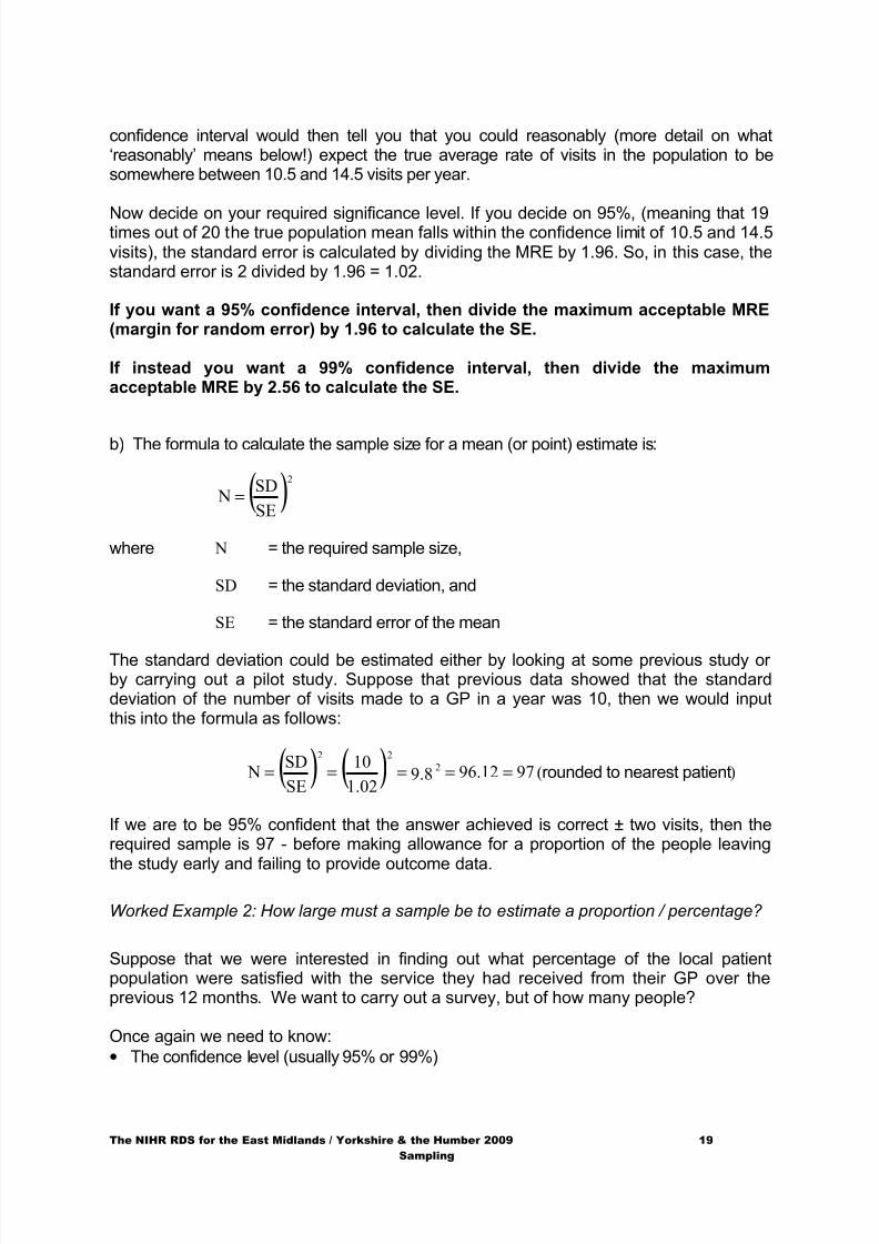
b) The formula to calculate the sample size for a mean (or point) estimate is:
( )SE
SD N
2
=
where N = the required sample size,
SD = the standard deviation, and
SE = the standard error of the mean
The standard deviation could be estimated either by looking at some previous study orby carrying out a pilot study. Suppose that previous data showed that the standarddeviation of the number of visits made to a GP in a year was 10, then we would inputthis into the formula as follows:
( ) ( ) 9712.969.81.02
10
SE
SD N 2
22
===== (rounded to nearest patient)
If we are to be 95% confident that the answer achieved is correct ± two visits, then therequired sample is 97 - before making allowance for a proportion of the people leaving
the study early and failing to provide outcome data.
Worked Example 2: How large must a sample be to estimate a proportion / percentage?
Suppose that we were interested in finding out what percentage of the local patientpopulation were satisfied with the service they had received from their GP over theprevious 12 months. We want to carry out a survey, but of how many people?
Once again we need to know:
• The confidence level (usually 95% or 99%)
8/21/2019 Hitung Sample Size
http://slidepdf.com/reader/full/hitung-sample-size 20/41
The NIHR RDS for the East Midlands / Yorkshire & the Humber 2009 20 Sampling
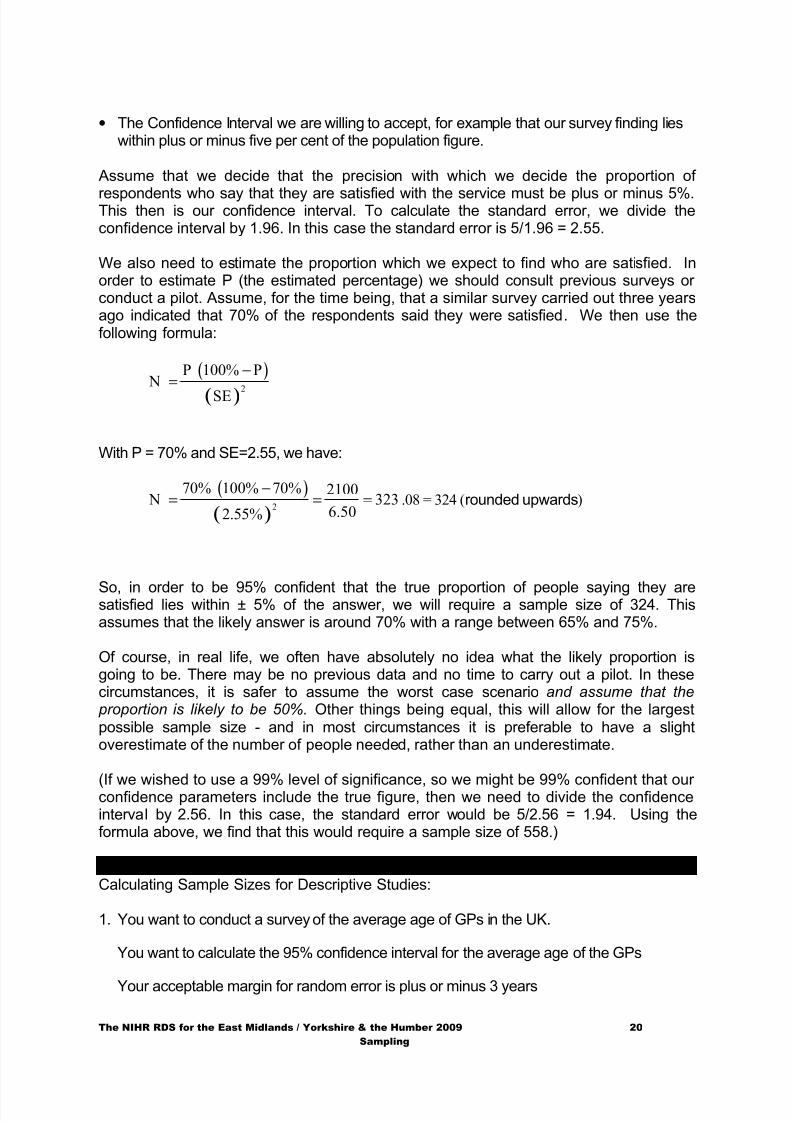
• The Confidence Interval we are willing to accept, for example that our survey finding lieswithin plus or minus five per cent of the population figure.
Assume that we decide that the precision with which we decide the proportion of
respondents who say that they are satisfied with the service must be plus or minus 5%.This then is our confidence interval. To calculate the standard error, we divide theconfidence interval by 1.96. In this case the standard error is 5/1.96 = 2.55.
We also need to estimate the proportion which we expect to find who are satisfied. Inorder to estimate P (the estimated percentage) we should consult previous surveys orconduct a pilot. Assume, for the time being, that a similar survey carried out three yearsago indicated that 70% of the respondents said they were satisfied. We then use thefollowing formula:
( )
( )2
P 100% P N
SE
−=
With P = 70% and SE=2.55, we have:
( )
( )2
70% 100% 70% 2100 N 323
6.502.55%
−= = = .08 = 324 (rounded upwards)
So, in order to be 95% confident that the true proportion of people saying they aresatisfied lies within ± 5% of the answer, we will require a sample size of 324. Thisassumes that the likely answer is around 70% with a range between 65% and 75%.
Of course, in real life, we often have absolutely no idea what the likely proportion isgoing to be. There may be no previous data and no time to carry out a pilot. In thesecircumstances, it is safer to assume the worst case scenario and assume that the proportion is likely to be 50%. Other things being equal, this will allow for the largestpossible sample size - and in most circumstances it is preferable to have a slightoverestimate of the number of people needed, rather than an underestimate.
(If we wished to use a 99% level of significance, so we might be 99% confident that ourconfidence parameters include the true figure, then we need to divide the confidenceinterval by 2.56. In this case, the standard error would be 5/2.56 = 1.94. Using theformula above, we find that this would require a sample size of 558.)
EXERCISE 4Calculating Sample Sizes for Descriptive Studies:
1. You want to conduct a survey of the average age of GPs in the UK.
You want to calculate the 95% confidence interval for the average age of the GPs
Your acceptable margin for random error is plus or minus 3 years
8/21/2019 Hitung Sample Size
http://slidepdf.com/reader/full/hitung-sample-size 21/41
The NIHR RDS for the East Midlands / Yorkshire & the Humber 2009 21 Sampling
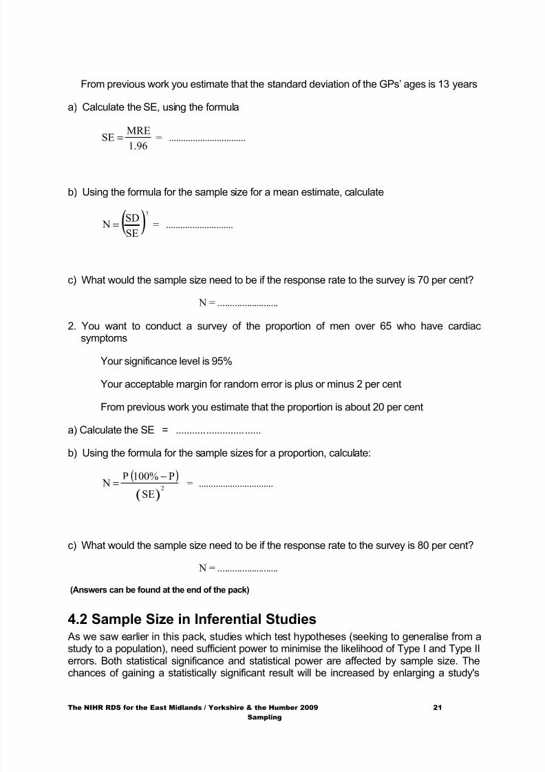
From previous work you estimate that the standard deviation of the GPs’ ages is 13 years
a) Calculate the SE, using the formula
1.96MRE SE = = ................................
b) Using the formula for the sample size for a mean estimate, calculate
( )SE
SD N
2
= = ............................
c) What would the sample size need to be if the response rate to the survey is 70 per cent?
N = .........................
2. You want to conduct a survey of the proportion of men over 65 who have cardiacsymptoms
Your significance level is 95%
Your acceptable margin for random error is plus or minus 2 per cent
From previous work you estimate that the proportion is about 20 per cent
a) Calculate the SE = ...............................
b) Using the formula for the sample sizes for a proportion, calculate:
( )
( )SE
P100%P N
2
−= = ...............................
c) What would the sample size need to be if the response rate to the survey is 80 per cent?
N = .........................
(Answers can be found at the end of the pack)
4.2 Sample Size in Inferential Studies As we saw earlier in this pack, studies which test hypotheses (seeking to generalise from astudy to a population), need sufficient power to minimise the likelihood of Type I and Type IIerrors. Both statistical significance and statistical power are affected by sample size. The
chances of gaining a statistically significant result will be increased by enlarging a study's
8/21/2019 Hitung Sample Size
http://slidepdf.com/reader/full/hitung-sample-size 22/41
The NIHR RDS for the East Midlands / Yorkshire & the Humber 2009 22 Sampling
sample. Put another way, the statistical power of a study is enhanced as sample sizeincreases. Let us look at each of these aspects of inferential research in turn. You may wishto refer back to Figure 1, on page 11.
The Statistical Significance of a StudyWhen a researcher uses a statistical test, what they are doing is testing their resultsagainst a gold standard. If the test gives a positive result (this is usually known as'achieving statistical significance'), then they can be relatively satisfied that their resultsare 'true', and that the real world situation is that discovered in the study (Cell 1 in Fig 1).If the test does not give significant results (non-significant or NS), then they can bereasonably satisfied that the results reflect Cell 4, where they have found no associationand no such association exists.
However, we can never be absolutely certain that we have a result which falls in Cells 1or 4. Statistical significance represents the likelihood of committing a Type I error (Cell 2).
Let us imagine that we have results suggesting an association between ill-health anddeprivation, and a t-test (a test to compare the results of two different groups) gives avalue which indicates that at the 5% or 0.05 level of statistical significance, there is moreill-health among a group of high scorers on the Jarman Index of deprivation than amonga group of low scorers.
What this means is that 95 per cent of the time, we can be certain that this result reflects atrue effect (Cell 1). Five per cent of the time, it is a chance result, resulting from randomassociations in the sample we chose. If the t-test value is higher, we might reach 1% or 0.01significance. Now, the result will only be a chance association one per cent of the time .
Tests of statistical significance are designed to account for sample size, thus the larger asample; the 'easier' it is for results to reach significance. A study which compares two groupsof 10 patients will have to demonstrate a much greater difference between the groups than astudy with 1000 patients in each group. This is fair: the larger study is much more likely to be'representative' of a population than the smaller one. To summarise: statistical significance isa measure of the likelihood that positive results reflect a real effect, and that the findings canbe used to make conclusions about differences which really exist.
The Statistical Power of a Study
Because of the way statistical tests are designed, as we have just seen, they build in asafety margin to avoid generalising false positive results which could have disastrous or
expensive consequences. But researchers who use small samples also run the risk ofnot being able to demonstrate differences or associations which really do exist. Thusthey are in danger of committing a Type II error (Cell 3 in Fig 1), of accepting a false nullhypothesis. Such studies are ‘under-powered’, not possessing sufficient statistical powerto detect the effects they set out to detect. Conventionally, the target is a power of 80%or 0.8 , meaning that a study has an 80 per cent likelihood of detecting a difference orassociation which really exists.
Examination of research undertaken in various fields of study suggests that manystudies do not meet this 0.8 conventional target for power (Fox and Mathers 1997).What this means is that many studies have a much reduced likelihood of being able todiscern the effects which they set out to seek: a study, with a power of 0.66 for some
8/21/2019 Hitung Sample Size
http://slidepdf.com/reader/full/hitung-sample-size 23/41
The NIHR RDS for the East Midlands / Yorkshire & the Humber 2009 23 Sampling
specified treatment effect, will only detect that effect (if true) two times out of three. Anon-significant finding of a study may thus simply reflect the inadequate power of thestudy to detect differences or associations at levels which are conventionally acceptedas statistically significant.
When a study has only small (say less than 50%) power to detect a useful result, one mustask the simple question of such research: ‘Why did you bother, when your study hadlittle chance of finding what you set out to find?’
Sample size calculations need to be undertaken prior to a study to avoid both thewasteful consequences of under-powering, (or of overpowering in which sample sizesare excessively large, with higher than necessary study costs and, perhaps, theneedless involvement of too many patients, which has ethical implications.).
Statistical power calculations are also sometimes undertaken after a study has beencompleted, to assess the likelihood of a study having discovered effects.
Statistical power is a function of three variables: sample size, the chosen level of
statistical significance (α) and effect size. While calculation of power entails recourse totables of values for these variables, the calculation is relatively straightforward in mostcases.
Effect Size and Sample Size
As was mentioned earlier, there is a trade-off between significance and power, becauseas one tries to reduce the chances of generating false negative results, the likelihood ofa false positive result increases. Researchers need to decide which is more crucial, andset the significance level accordingly. In Exercise 3 you were asked to decide, in various
situations, whether a Type I or Type II error was more serious - based on clinical andother criteria.
Fortunately both statistical significance and power are increased by increasing sample size,so increasing sample size will reduce likelihoods of both Type I and Type II errors. However,that does not mean that researchers necessarily need to vastly increase the size of theirsamples, at great expense of time and resources.
The other factor affecting the power of a study is the effect size (ES) which is underinvestigation in the study. This is a measure of ‘how wrong the null hypothesis is’. Forexample, we might compare the efficacy of two bronchodilators for treating an asthma
attack. The ES is the difference in efficacy between the two drugs. An effect size may bea difference between groups or the strength of an association between variables such asill-health and deprivation.
If an ES is small, then many studies with small sample sizes are likely to be under-powered. But if an ES is large, then a relatively small scale study could have sufficientpower to identify the effect under investigation. It is sometimes possible to increase theeffect size (for example, by making more extreme comparisons, or undertaking a longeror more powerful intervention), but usually this is the intractable element in the equation,and accurate estimation of the effect size is essential for calculating power before astudy begins, and hence the necessary sample size.
8/21/2019 Hitung Sample Size
http://slidepdf.com/reader/full/hitung-sample-size 24/41
The NIHR RDS for the East Midlands / Yorkshire & the Humber 2009 24 Sampling
An Effect Size can be estimated in two ways:
Preferably:
• One can make a decision about the smallest size of effect which it is worth identifying . Toconsider the example of two rival drugs, if we are willing to accept the two drugs asequivalent if there is no more than a ten per cent difference in their efficacy of treatment,then this effect size may be set, acknowledging that smaller effects will not be discernible.
Alternatively:
• From a review of literature or meta-analysis, which can suggest the size of ES which maybe expected.
4.3 A case study of statistical power: primary care researchPower calculations may be used as part of the critical appraisal of research papers.Unfortunately it is rare to see values for statistical power quoted for tests in researchreports, and indeed often the results reported are inadequate to calculate effect sizes. Appraisals of various scientific subjects including nursing, education, management andgeneral practice research have been undertaken by various authors.
Now read the edited extract from an article by Nick Fox and Nigel Mathers (1997).
Empowering your research: statistical power in general practice research
Fami ly Practice 14 (4) 1997
To explore the power of general practice research, we analysed all the statistical testsreported in the British Journal of General Practice (BJGP) over a period of 18 months.Power was calculated for each test based on the reported sample size. This enabledcalculation of the power of each quantitative study published during this period, toassess the adequacy of sample sizes to supply sufficient power.
Method
All original research papers published in the BJGP during the period January 1994 to
June 1995 inclusive were analysed in terms of the power of statistical tests reported.Qualitative papers were excluded, as were meta-analyses and articles which, althoughreporting quantitative data, did not report any formal statistical analysis even though insome instances such tests could have been undertaken. A further six papers wereexcluded because they did not use standard statistical tests for which power tables wereavailable. This left 85 papers, involving 1422 tests for which power could be calculatedusing power tables. Power was calculated for each test following conventions of similarresearch into statistical power. Where adequate data was available (for example detailsof group means and standard deviations, or chi-squared test results) precise effect sizescould be calculated. Where this was not possible (in particular for results simply reportedas ‘non-significant’) the following assumptions were made, all of which considerably
over-estimate the power of the test:
8/21/2019 Hitung Sample Size
http://slidepdf.com/reader/full/hitung-sample-size 25/41
The NIHR RDS for the East Midlands / Yorkshire & the Humber 2009 25 Sampling
a) For significant results, the effect size was assumed to be `medium’, which as noted earliermeans an effect `visible to the naked eye’. Non-significant results were assumed to havea ‘small’ ES.
b) Alpha values were set at the lowest possible conventional level of 0.05, and where adirectional test was used, a one-tailed alpha was used (equivalent to two-tailed alpha of0.1).
From the calculations of power for individual tests, a mean power for each paper wasderived. This strategy has been adopted in other research into statistical power: what isreported is study power, rather than test-by-test power, and offers an estimate of thequality of studies in terms of overall adequacy of statistical power.
Results
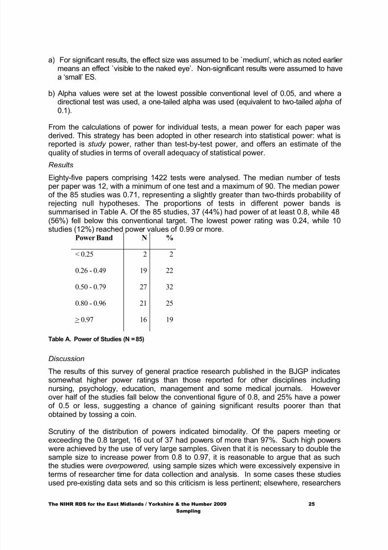
Eighty-five papers comprising 1422 tests were analysed. The median number of testsper paper was 12, with a minimum of one test and a maximum of 90. The median power
of the 85 studies was 0.71, representing a slightly greater than two-thirds probability ofrejecting null hypotheses. The proportions of tests in different power bands issummarised in Table A. Of the 85 studies, 37 (44%) had power of at least 0.8, while 48(56%) fell below this conventional target. The lowest power rating was 0.24, while 10studies (12%) reached power values of 0.99 or more.
Power Band N %
< 0.25 2 2
0.26 - 0.49 19 22
0.50 - 0.79 27 32
0.80 - 0.96 21 25
> 0.97 16 19
Table A. Power of Studies (N = 85)
Discussion
The results of this survey of general practice research published in the BJGP indicatessomewhat higher power ratings than those reported for other disciplines includingnursing, psychology, education, management and some medical journals. Howeverover half of the studies fall below the conventional figure of 0.8, and 25% have a powerof 0.5 or less, suggesting a chance of gaining significant results poorer than thatobtained by tossing a coin.
Scrutiny of the distribution of powers indicated bimodality. Of the papers meeting orexceeding the 0.8 target, 16 out of 37 had powers of more than 97%. Such high powerswere achieved by the use of very large samples. Given that it is necessary to double thesample size to increase power from 0.8 to 0.97, it is reasonable to argue that as suchthe studies were overpowered, using sample sizes which were excessively expensive interms of researcher time for data collection and analysis. In some cases these studies
used pre-existing data sets and so this criticism is less pertinent; elsewhere, researchers
8/21/2019 Hitung Sample Size
http://slidepdf.com/reader/full/hitung-sample-size 26/41
The NIHR RDS for the East Midlands / Yorkshire & the Humber 2009 26 Sampling
may have devoted far greater efforts in terms of time and obtaining goodwill fromsubjects than may strictly have been necessary to achieve adequate power. Theimportance of pre-study calculations of necessary sample size to achieve statisticalpower of 0.8 or thereabouts is relevant both for those studies demonstrated to be under-
powered and those for whom power is excessive.Conclusions
More than half of the quantitative papers published in the BJGP between January 1994 toJune 1995 were `under-powered’. This means that during the statistical analysis, there was asubstantial risk of missing significant results. Twenty five percent of papers surveyed had achance of gaining significant results (when there was a false null hypothesis) poorer than thatobtained from tossing a coin.
EXERCISE 5What was the median power of research in the papers surveyed?What proportion of papers had too high a power - of, say, at least 99% - and why is thisan issue?
(Answers can be found at the end of the pack)
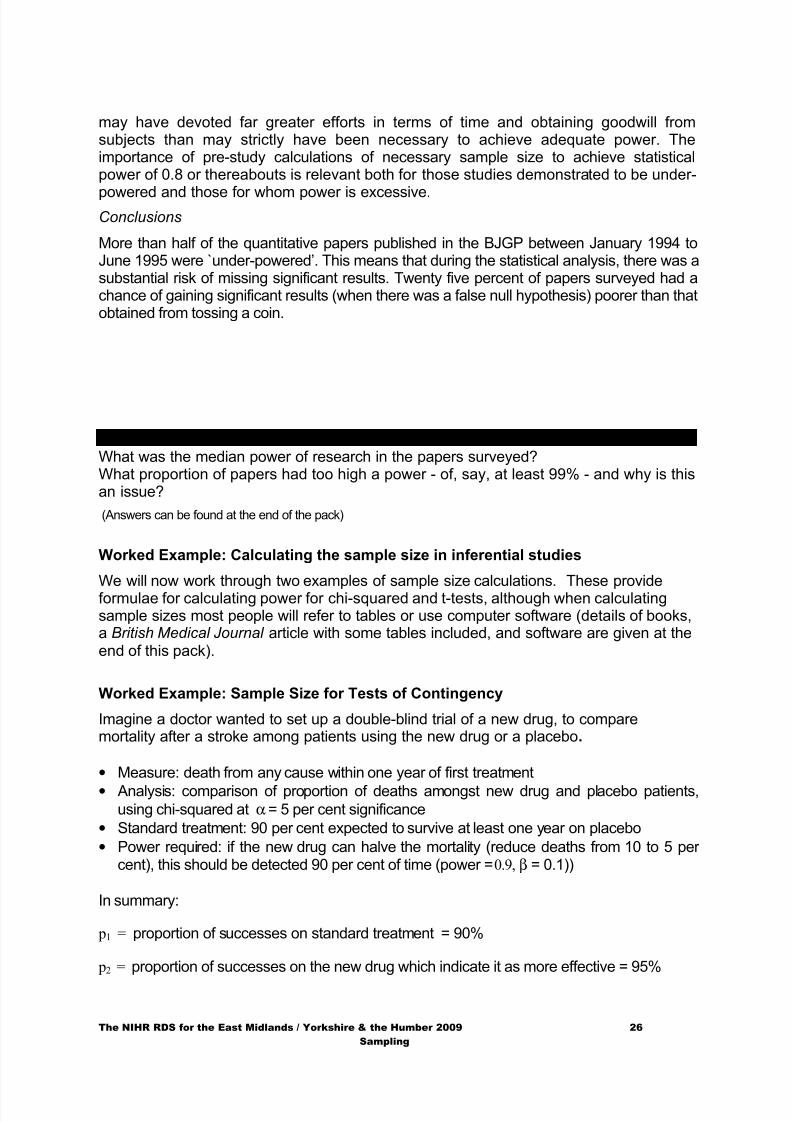
Worked Example: Calculating the sample size in inferential studies
We will now work through two examples of sample size calculations. These provideformulae for calculating power for chi-squared and t-tests, although when calculatingsample sizes most people will refer to tables or use computer software (details of books,a British Medical Journal article with some tables included, and software are given at theend of this pack).
Worked Example: Sample Size for Tests of Contingency
Imagine a doctor wanted to set up a double-blind trial of a new drug, to comparemortality after a stroke among patients using the new drug or a placebo .
• Measure: death from any cause within one year of first treatment
• Analysis: comparison of proportion of deaths amongst new drug and placebo patients,using chi-squared at α = 5 per cent significance
• Standard treatment: 90 per cent expected to survive at least one year on placebo
• Power required: if the new drug can halve the mortality (reduce deaths from 10 to 5 percent), this should be detected 90 per cent of time (power = 0.9, β = 0.1))
In summary:
p1 = proportion of successes on standard treatment = 90%
p2 = proportion of successes on the new drug which indicate it as more effective = 95%
8/21/2019 Hitung Sample Size
http://slidepdf.com/reader/full/hitung-sample-size 27/41
The NIHR RDS for the East Midlands / Yorkshire & the Humber 2009 27 Sampling
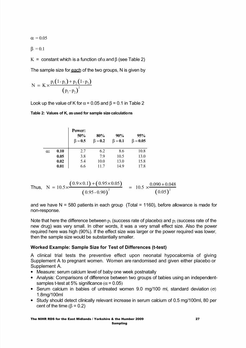
α = 0.05
β = 0.1
K = constant which is a function of α and β (see Table 2)
The sample size for each of the two groups, N is given by
( ) ( )
( ) p- p
p-1 p p-1 pK N
21
2
2211 +
×=
Look up the value of K for α = 0.05 and β = 0.1 in Table 2
Table 2: Values of K, as used for sample size calculations
Power:50% 80% 90% 95%
β = 0.5 β = 0.2 β = 0.1 β = 0.05
α: 0.10 2.7 6.2 8.6 10.8
0.05 3.8 7.9 10.5 13.0
0.02 5.4 10.0 13.0 15.8
0.01 6.6 11.7 14.9 17.8
Thus, ( ) ( )
( )0.90-0.95
05.00.950.10.9 10.5 N
2
×+××= ( )
2
0.090 0.048 10.5
0.05
+= ×
and we have N = 580 patients in each group (Total = 1160), before allowance is made fornon-response.
Note that here the difference between p1 (success rate of placebo) and p2 (success rate of thenew drug) was very small. In other words, it was a very small effect size. Also the powerrequired here was high (90%). If the effect size was larger or the power required was lower,then the sample size would be substantially smaller.
Worked Example: Sample Size for Test of Differences (t-test)
A clinical trial tests the preventive effect upon neonatal hypocalcemia of givingSupplement A to pregnant women. Women are randomised and given either placebo orSupplement A.
• Measure: serum calcium level of baby one week postnatally
• Analysis: Comparisons of difference between two groups of babies using an independent-
samples t-test at 5% significance (α = 0.05)
• Serum calcium in babies of untreated women 9.0 mg/100 ml, standard deviation (σ)
1.8mg/100ml
• Study should detect clinically relevant increase in serum calcium of 0.5 mg/100ml, 80 per
cent of the time (β = 0.2)
8/21/2019 Hitung Sample Size
http://slidepdf.com/reader/full/hitung-sample-size 28/41
The NIHR RDS for the East Midlands / Yorkshire & the Humber 2009 28 Sampling
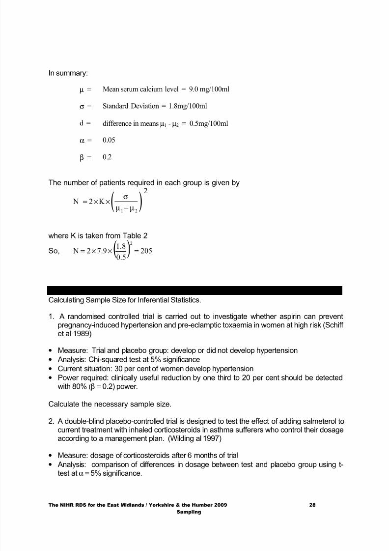
In summary:
µ = Mean serum calcium level = 9.0 mg/100ml
σ = Standard Deviation = 1.8mg/100ml
d = difference in means µ1 - µ2 = 0.5mg/100ml
α = 0.05
β = 0.2
The number of patients required in each group is given by
( )
1 2
2 N 2 K
σ
µ µ= × ×
−
where K is taken from Table 2
So, ( ) 2055.0
8.17.92 N
2
=××=
EXERCISE 6Calculating Sample Size for Inferential Statistics.
1. A randomised controlled trial is carried out to investigate whether aspirin can preventpregnancy-induced hypertension and pre-eclamptic toxaemia in women at high risk (Schiffet al 1989)
• Measure: Trial and placebo group: develop or did not develop hypertension
• Analysis: Chi-squared test at 5% significance
• Current situation: 30 per cent of women develop hypertension
• Power required: clinically useful reduction by one third to 20 per cent should be detected
with 80% (β = 0.2) power .
Calculate the necessary sample size.
2. A double-blind placebo-controlled trial is designed to test the effect of adding salmeterol tocurrent treatment with inhaled corticosteroids in asthma sufferers who control their dosageaccording to a management plan. (Wilding al 1997)
• Measure: dosage of corticosteroids after 6 months of trial
• Analysis: comparison of differences in dosage between test and placebo group using t-test at α = 5% significance.
8/21/2019 Hitung Sample Size
http://slidepdf.com/reader/full/hitung-sample-size 29/41
The NIHR RDS for the East Midlands / Yorkshire & the Humber 2009 29 Sampling
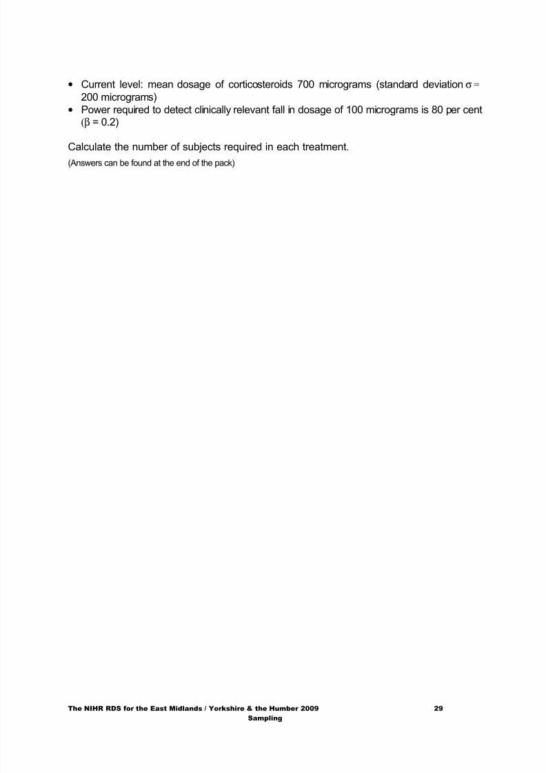
• Current level: mean dosage of corticosteroids 700 micrograms (standard deviation σ =
200 micrograms)
• Power required to detect clinically relevant fall in dosage of 100 micrograms is 80 per cent (β = 0.2)
Calculate the number of subjects required in each treatment.
(Answers can be found at the end of the pack)
8/21/2019 Hitung Sample Size
http://slidepdf.com/reader/full/hitung-sample-size 30/41
The NIHR RDS for the East Midlands / Yorkshire & the Humber 2009 30 Sampling
5. Summary
Key points to remember when deciding on sample selection are:
• Try to use a random method where possible and remember that random does notmean ‘haphazard’ or ‘arbitrary’.
• Random selection means that everybody in your sampling frame has an equalopportunity of being included in your study.
• If you need to be able to generalise about small or minority groups and to comparethose with larger groups, consider using disproportionate stratified sampling, butremember to re-weight the results afterwards if you wish to generalise to the wholepopulation.
Key points to remember when deciding on sample size are:
• We strongly recommend that researchers obtain independent advice on samplesize when designing their study - and this will usually be from either a trainedstatistician or from a researcher in your field who has longstanding experience ofstudy design.This is because sample size estimation is such a crucial aspect of the design of aquantitative study, with important ethical as well as cost implications - and oftenvery little can be done to ‘salvage’ the results from an insufficiently large sample.
• There is a trade off between committing a Type I error (false positive) and a Type IIerror (false negative), but historically science has placed the emphasis on avoidingType I errors.
• Other things being equal, increasing the sample size increases the sensitivity ofthe study to detect a difference between the groups being compared - and enables
both α and β to be set at lower levels, and so will help reduce both Type I and
Type II errors, but remember that it is costly and unethical to have too large asample size.
• To calculate statistical power, you need to estimate the effect size.
• To estimate the sample size for a descriptive study in order to estimate a mean ora proportion, it is necessary to specify the maximum acceptable margin for randomerror.
8/21/2019 Hitung Sample Size
http://slidepdf.com/reader/full/hitung-sample-size 31/41
The NIHR RDS for the East Midlands / Yorkshire & the Humber 2009 31 Sampling
6. Answers to exercises
Exercise 1
1. Stratified random sample. The sample is stratified because the sample has beenselected to ensure that two different groups are represented.
2. Disproportionate stratified random sample. This sample is stratified to ensure that
equal numbers of children from the two groups are selected - even though, in thepopulation, only a relatively small proportion of children suffer from chronic asthma.The total sample with therefore not be representative of the children in the population.
3. Quota. The sample is not randomly selected but the respondents are selected to
meet certain criteria.
4. Convenience. The sample is not randomly selected and no quotas are applied.
5. Systematic random sample.
6. Cluster sample. The patients are selected only from certain wards - and whether
this is a randomised or a convenience cluster sample depends on how these wardshad been chosen.
Exercise 2
1. The researchers used a convenience sampling approach, i.e. they selected people
on the basis that they were easy to access. Respondents were therefore self-selected.
2. The sampling method used was non-random.
3. The advantages of this approach were that they were able to obtain the views of a
large number of people very quickly and easily with little expense.
4. Unfortunately the convenience sample approach means that the sample is not
representative of the population of individuals with asthma. Because a large part ofthe survey is made up of people attending in surgery and pharmacies, the sample willtend to over-represent those individuals requiring the most treatment. It will also over-represent those individuals who are most interested in expressing their opinions.
5. The sample achieved was very large because it was self-selected, and therefore
the researchers would have had little control over how many people participated.
The sample is unnecessarily large. In order to achieve a statistically representativeview of the asthmatic population, it would not be necessary to select such a largesample. This study demonstrates the point that large samples alone do notnecessarily mean that the study can achieve representativeness. The only true wayof achieving a representative sample is to use random sampling methods. Reflect onthe sample size in this study as you now go on to study the second part of this pack.
8/21/2019 Hitung Sample Size
http://slidepdf.com/reader/full/hitung-sample-size 32/41
The NIHR RDS for the East Midlands / Yorkshire & the Humber 2009 32 Sampling
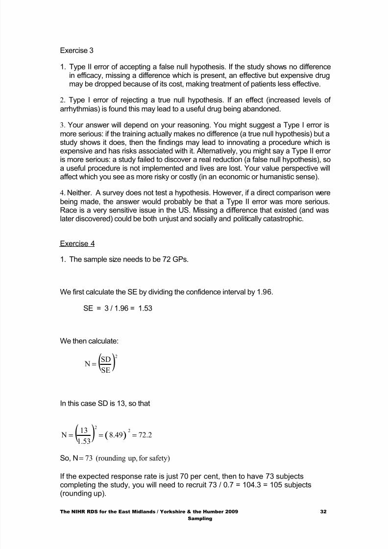
Exercise 3
1. Type II error of accepting a false null hypothesis. If the study shows no differencein efficacy, missing a difference which is present, an effective but expensive drugmay be dropped because of its cost, making treatment of patients less effective.
2. Type I error of rejecting a true null hypothesis. If an effect (increased levels of
arrhythmias) is found this may lead to a useful drug being abandoned.
3. Your answer will depend on your reasoning. You might suggest a Type I error is
more serious: if the training actually makes no difference (a true null hypothesis) but astudy shows it does, then the findings may lead to innovating a procedure which isexpensive and has risks associated with it. Alternatively, you might say a Type II erroris more serious: a study failed to discover a real reduction (a false null hypothesis), soa useful procedure is not implemented and lives are lost. Your value perspective willaffect which you see as more risky or costly (in an economic or humanistic sense).
4. Neither. A survey does not test a hypothesis. However, if a direct comparison werebeing made, the answer would probably be that a Type II error was more serious.Race is a very sensitive issue in the US. Missing a difference that existed (and waslater discovered) could be both unjust and socially and politically catastrophic.
Exercise 4
1. The sample size needs to be 72 GPs.
We first calculate the SE by dividing the confidence interval by 1.96.
SE = 3 / 1.96 = 1.53
We then calculate:
( )SE
SD N
2
=
In this case SD is 13, so that
( ) ( ) 72.28.491.53
13 N
22
===
So, N safety)forup,(rounding 73=
If the expected response rate is just 70 per cent, then to have 73 subjectscompleting the study, you will need to recruit 73 / 0.7 = 104.3 = 105 subjects(rounding up).
8/21/2019 Hitung Sample Size
http://slidepdf.com/reader/full/hitung-sample-size 33/41
The NIHR RDS for the East Midlands / Yorkshire & the Humber 2009 33 Sampling
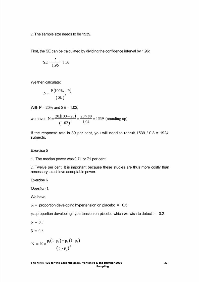
2. The sample size needs to be 1539.
First, the SE can be calculated by dividing the confidence interval by 1.96:
02.11.96
2 SE ==
We then calculate:
( )
( )SE
P100%P N
2
−=
With P = 20% and SE = 1.02,
we have: ( )
( )up)(rounding 1539
04.1
8020
1.02
2010020. N
2 =
×=
−=
If the response rate is 80 per cent, you will need to recruit 1539 / 0.8 = 1924subjects.
Exercise 5
1. The median power was 0.71 or 71 per cent.
2. Twelve per cent. It is important because these studies are thus more costly thannecessary to achieve acceptable power.
Exercise 6
Question 1.
We have:
p1 = proportion developing hypertension on placebo = 0.3
p2 = proportion developing hypertension on placebo which we wish to detect = 0.2
α = 0.5
β = 0.2
( ) ( )
( ) p- p
p-1 p p-1 pK N
21
2
2211 +
×=
8/21/2019 Hitung Sample Size
http://slidepdf.com/reader/full/hitung-sample-size 34/41
The NIHR RDS for the East Midlands / Yorkshire & the Humber 2009 34 Sampling
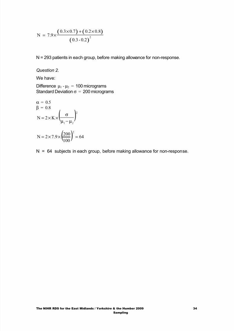
( ) ( )
( )0.2-0.3
8.00.20.70.3 7.9 N
2
×+××=
N = 293 patients in each group, before making allowance for non-response.
Question 2.
We have:
Difference µ1 - µ2 = 100 micrograms
Standard Deviation σ = 200 micrograms
α = 0.5
β = 0.8
µµ
σ
21
2
K 2 N−
××=
( ) 64100
2007.92 N
2
=××=
N = 64 subjects in each group, before making allowance for non-response.

8/21/2019 Hitung Sample Size
http://slidepdf.com/reader/full/hitung-sample-size 35/41
The NIHR RDS for the East Midlands / Yorkshire & the Humber 2009 35 Sampling
7. Further reading and resources
For details of sampling techniques
V Barnett. (2002) Sample survey - Principles and methods. 3rd edition Publ: Hodder Arnold
Bland M. (2000) An Introduction to Medical Statistics. 3rd edition. Oxford: UniversityPress
For details of power calculations
Campbell MJ, Julious SA and Altman DG (1995) ‘Estimating sample sizes for binary,ordered categorical and continuous outcomes in two group comparisons’ BMJ 311:1145-8.
Petrie A and Samib C. (2005) Medical Statistics at a Glance. 2nd edition. Oxford:Blackwell Publishing.
Machin D, Campbell MJ. (1997) Sample Size Tables for Clinical Studies. 2nd edition.Oxford: Blackwell Scientific.
The software package nQuery Advisor provides simple efficient means of calculatingpower and sample size. It may be obtained from Statistical Solutions (8 South Bank,Crosse’s Green, Cork, Ireland. Tel: 00 353 21 319629; Fax: 00 353 21 319630, e-mail: [email protected]).
More details are available from http://www.statsol.ie/html/nquery/nquery_home.html
The software Epi Info also provides information on calculating sample sizes and canbe obtained for little or no charge from either your local Public Health Department orfrom your local academic department of general practice or from your local auditadvisory group. More details are available from http://www.cdc.gov/EpiInfo/
Studies of power in different scientific disciplines
Fox NJ, Mathers NJ. (1997) ‘Empowering your research: statistical power in generalpractice research’. Family Practice 14 (4): 324-329.
Polit DF, Sherman RE. (1990) ‘Statistical power in nursing research’. Nursing
Research 39: 365-369.
Reed JF, Slaichert W. (1981) ‘Statistical proof in inconclusive “negative” trials’. Archives of Internal Medicine 141: 1307-1310.
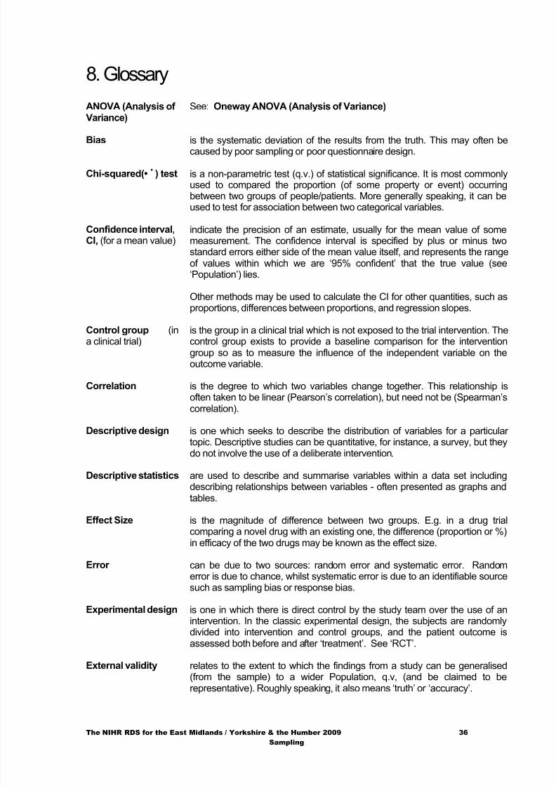
8/21/2019 Hitung Sample Size
http://slidepdf.com/reader/full/hitung-sample-size 36/41
The NIHR RDS for the East Midlands / Yorkshire & the Humber 2009 36 Sampling
8. Glossary
ANOVA (Analysis ofVariance)
See: Oneway ANOVA (Analysis of Variance)
Bias is the systematic deviation of the results from the truth. This may often becaused by poor sampling or poor questionnaire design.
Chi-squared(••) test is a non-parametric test (q.v.) of statistical significance. It is most commonly
used to compared the proportion (of some property or event) occurringbetween two groups of people/patients. More generally speaking, it can beused to test for association between two categorical variables.
Confidence interval,CI, (for a mean value)
indicate the precision of an estimate, usually for the mean value of somemeasurement. The confidence interval is specified by plus or minus twostandard errors either side of the mean value itself, and represents the rangeof values within which we are ‘95% confident’ that the true value (see
‘Population’) lies.
Other methods may be used to calculate the CI for other quantities, such asproportions, differences between proportions, and regression slopes.
Control group (ina clinical trial)
is the group in a clinical trial which is not exposed to the trial intervention. Thecontrol group exists to provide a baseline comparison for the interventiongroup so as to measure the influence of the independent variable on theoutcome variable.
Correlation is the degree to which two variables change together. This relationship isoften taken to be linear (Pearson’s correlation), but need not be (Spearman’s
correlation).
Descriptive design is one which seeks to describe the distribution of variables for a particulartopic. Descriptive studies can be quantitative, for instance, a survey, but theydo not involve the use of a deliberate intervention.
Descriptive statistics are used to describe and summarise variables within a data set includingdescribing relationships between variables - often presented as graphs andtables.
Effect Size is the magnitude of difference between two groups. E.g. in a drug trialcomparing a novel drug with an existing one, the difference (proportion or %)in efficacy of the two drugs may be known as the effect size.
Error can be due to two sources: random error and systematic error. Randomerror is due to chance, whilst systematic error is due to an identifiable sourcesuch as sampling bias or response bias.
Experimental design is one in which there is direct control by the study team over the use of anintervention. In the classic experimental design, the subjects are randomlydivided into intervention and control groups, and the patient outcome isassessed both before and after ‘treatment’. See ‘RCT’.
External validity relates to the extent to which the findings from a study can be generalised(from the sample) to a wider Population, q.v, (and be claimed to be
representative). Roughly speaking, it also means ‘truth’ or ‘accuracy’.
8/21/2019 Hitung Sample Size
http://slidepdf.com/reader/full/hitung-sample-size 37/41
The NIHR RDS for the East Midlands / Yorkshire & the Humber 2009 37 Sampling
Frame see ‘Sampling frame’
Hypothesis a statement about the relationship between the dependent (i.e. outcome) andthe independent (i.e. predictor, or explanatory) variables to be studied.Traditionally the null hypothesis is assumed to be correct, until researchdemonstrates that the null hypothesis is incorrect. See ‘null hypothesis’.
Incidence can be defined as the number of new occurrences of a phenomenon e.g.illness, in a defined population within a specified period of time. An incidencerate would be the rate at which new cases of the phenomenon occur in agiven population. Also see ‘prevalence’.
Independent variable also sometimes known as a ‘predictor’ or ‘explanatory’ variable. Our interestin a study is usually in the association between one or more independentvariables, and the ‘dependent’ or outcome variable (q.v.). In an experimentsuch as a clinical trial, the independent variable takes the form of theintervention or treatment, and is manipulated to demonstrate change in thedependent variable.
Inferential statistics is the whole family of statistical techniques used to make generalisationsfrom a sample to a population.
Internal validity relates to the validity of the study itself, including both the design and theinstruments used. Roughly speaking, this means ‘internal consistency’.
Intervention is the independent variable in an experimental design. An intervention couldtake the form of treatment, such as drug or surgical treatment. Thosesubjects selected to receive the intervention in an experiment are placed inthe ‘intervention’ group.
Mean is the ‘average’ value of a measurement. It is calculated by summing all theindividual values and dividing this figure by the total number of individualcases to produce a mean average. It is a descriptive statistic which shouldonly be applied to data on an ‘interval’ scale.
Median is another measure of central tendency. It is the mid-point or middle valuewhere all the values are placed in order. It is less susceptible to distortion byextreme values than the mean, and is a suitable descriptive statistic for bothordinal and interval data. It is the basis of nonparametric statistics (q.v.).
Mode is the most frequently occurring of a number of mutually exclusive categoriesinto which the study patients/subjects are divided. N.B. the ‘mode’ can bemisleading when applied to numerical/quantitative data.
Nominal data, also known as categorical data, is a set of unordered categories. Eachcategory may sometimes be represented using a different numerical code,but the codes or numbers are allocated on an arbitrary basis and have nonumerical meaning. See also ‘ordinal’ and ‘interval data’.
Non-parametricstatistics,
unlike parametric statistics, do not make any assumptions about theunderlying distribution of data. Non-parametric statistics are therefore suitablefor skewed data and nominal and ordinal levels of measurement.
Null hypothesis is a hypothesis (q.v.), and is usually chosen to ‘say’ that there is norelationship between the dependent and independent variables. The null
hypothesis is assumed to be correct, until research demonstrates that it is
8/21/2019 Hitung Sample Size
http://slidepdf.com/reader/full/hitung-sample-size 38/41
The NIHR RDS for the East Midlands / Yorkshire & the Humber 2009 38 Sampling
incorrect.
Oneway ANOVA (Analysis ofVariance)
is a test of statistical significance for assessing the difference between two ormore sample means. Also known as F test.
Ordinal data is composed of a set of categories which can be placed in an order. Eachcategory is represented by a numeric code which in turn represents the sameorder as the data. However, the numbers do not represent the distancebetween each category. For instance, a variable describing patientsatisfaction may be coded as follows: Dissatisfied 1, Neither 2, Satisfied 3.The code 2 cannot be interpreted as having twice the value of code 1.
Parametric statistics are generally based on the assumption that the data follows a Normaldistribution, i.e. the data when plotted follows a bell-shaped curve. Examplesof parametric statistics are t-tests and analysis of variance (ANOVA).
Panel study is another term for a longitudinal, cohort, or ‘repeated measures’ study,
where individuals are examined and assessed repeatedly over a period oftime.
Parallel design refers to the traditional experimental design where each study subject/patientis allocated to just a single study treatment. An alternative to a parallel designis a ‘crossover’ design.
Placebo is usually an inert drug or ‘sugar coated pill’ used to simulate drug treatmentin a control group in an experimental design. Placebo is Latin for ‘I willplease’.
Population is a term used in research which refers to all the potential subjects or units ofinterest who share the same characteristics which would make them eligiblefor entry into a study. The population of potential subjects is also known asthe sampling frame.
Power of a study is the probability of showing a difference between two groups,when there is a real difference of a pre-specified size between thecorresponding populations. Therefore increasing the power of a study willreduce the chance of committing a Type II error. Power calculations are usedto find out how likely we are to detect an effect for a given sample size, effectsize, and level of significance. Power is usually denoted as 1 - • . Theminimum recommended power level is 80%.
Prevalence Is the number of cases or subjects with a given condition or disease within a
specified time period. The prevalence of a condition would include all thosepeople with the condition even if the condition started prior to the start of thespecified time period. Compare with Incidence.
Prospective study is one that is planned from the beginning and takes a forward lookingapproach. Subjects are followed over time and interventions can beintroduced as appropriate. Compare with ‘Retrospective’.
Qualitative research usually dealing with the human experience and which is based onanalysis of words rather than numbers. Qualitative research methods seek toexplore rich information usually collected from fairly small samples andinclude methods such as in-depth interviews, focus groups, action research
and ethnographic studies.
8/21/2019 Hitung Sample Size
http://slidepdf.com/reader/full/hitung-sample-size 39/41
The NIHR RDS for the East Midlands / Yorkshire & the Humber 2009 39 Sampling
Quantitative research is essentially concerned with numerical measurement andnumerical data. All experimental research is based on a quantitativeapproach. Quantitative research tends to be based on larger sample sizes inorder to produce results which can be generalised to a wider population.
Quasi-experimental
design
is one in which the researcher has no control over who receives the
intervention and who does not. An alternative to randomisation as used inexperimental research, is the process of matching.
Quota sample is a form of non-random sampling and one that is commonly used in marketresearch. The sample is designed to meet certain quotas, set usually toobtain certain numbers by age, sex and social class. The sample selectedwithin each quota is selected by convenience, rather than random methods.
Randomisation is the random assignment of subjects to intervention and control groups.Randomisation is a way of ensuring that chance dictates who receives whichtreatment. In this way all extraneous variables should be controlled for.Random allocation does not mean haphazard allocation.
Random error is non-systematic bias which can negate the influence of the independentvariable. Reliability is affected by random error.
Randomised controltrial (RCT)
is seen as the ‘gold standard’ of experimental design. As the name impliessubjects are randomly allocated to either the intervention or the control group.
Ratio level data is similar to interval data in that there is an equal distance between eachvalue except that ratio data does possess a true zero. An example of ratiodata would be age.
Reliability is concerned with the extent to which a measure gives consistent results. It isalso a pre-condition for validity.
Representativeness is the extent to which a sample of subjects is representative of the widerpopulation. If a sample is not representative, then the findings may not begeneralisable.
Response rate is the proportion of people who have participated in a study, or who havecompleted a question / questionnaire. It is calculated by dividing the totalnumber of people who have participated by those who were approached orasked to participate.
Retrospective study is a study in which the ‘outcome’ (the event or characteristic recorded by the‘Independent variable’) of study subjects/patients may have already
happened before the study was planned - and is typically found from recordssuch as patient notes. Compare with ‘Prospective’.
Sample is the group or subset of the study ‘Population’ that is recruited for the study. A sample can be selected by random or non-random methods. Findings froma representative sample can be generalised to the wider population. N.B.sometimes each treatment group in a study is referred to as a ‘sample’, andso the ‘total sample’ is the combination of these treatment groups of studysubjects.
Sampling frame is the pool of potential subjects who share similar criteria for entry in to astudy. The sampling frame is also known as the ‘population’. An example
might be: all people who suffered a stroke during the calendar year 2005
8/21/2019 Hitung Sample Size
http://slidepdf.com/reader/full/hitung-sample-size 40/41
The NIHR RDS for the East Midlands / Yorkshire & the Humber 2009 40 Sampling
while resident in the UK.
Significance level usually means the highest value for ‘P-value’ in statistical test that will beconsidered to be significant. The significance level is commonly set at either0.01 (giving a one in a hundred chance of giving a ‘false positive’ test result)or 0.05 (a corresponding chance of one in twenty chance).
Significance tests may be parametric or non-parametric. A significance test is used to detectdifferences between groups or associations between variables that are toogreat to have reasonably occurred by chance. The result is recorded as a P-value - or as statistical significance, according to some pre-set Significancelevel (q.v.).
Snowballing is a non-probability method of sampling commonly employed in qualitativeresearch. Recruited subjects nominate other potential subjects for inclusion inthe study.
Spurious correlation is an apparent correlation between two variables when there is no causal link
between them. Spurious relationships are often accounted for by a thirdconfounding variable. Once this third variable is controlled, the correlationbetween the two variables disappears. Another term for this is ‘artifact’.
SPSS (Statistical Package for the Social Sciences) is a popular and easy-to-usemenu-driven software package for data analysis - its main limitation is that insome common situations, it is difficult or impossible to obtain 95% confidenceintervals for your study results.
Standard deviation is a summary measure of ‘dispersion’, i.e. of the variability of a set ofmeasurements. It is a summary of how closely clustered or dispersed thevalues are around the mean. For data that is normally distributed, 68% of allcases lay within one standard derivation either side of the mean and 95% ofall cases are within two standard deviations either side of the mean.
Standard error is the standard deviation of an estimate of some quantity.
Stratified sample is one where the sample is divided up in to a number of different strata basedon certain criteria such as age or sex or ethnic group. The sample selectionwithin each strata is however based on a random or systematic samplingmethod. A stratified sample is a way of ensuring that the sample isrepresentative rather than leaving it to chance.
Survey is a method of collecting large scale quantitative data, but it does not use anexperimental design. With a survey there is no control over e.g. who receivesa medical intervention or when - but the corresponding advantage is that theresearcher can examine the ‘real world’ and describe existing relationships.
Theoretical sampling see the RDSU Resource Pack on Qualitative Research Methods.
Type I error is the error of falsely rejecting a true null hypothesis and thereby acceptingthat there is a statistical difference when one does not exist. When designinga study, the acceptable chance of committing a Type I error is known asalpha.
Type II error is the error of failing to reject a false null hypothesis or wrongly accepting afalse null hypothesis. The likelihood of committing a Type II error, for e.g. a
8/21/2019 Hitung Sample Size
http://slidepdf.com/reader/full/hitung-sample-size 41/41
treatment of a pre-specified size, is known as beta (• ). The conventionallevel of statistical power (1- • ) and is usually set at 80% or 0.8.
t-test is a test of statistical significance for assessing the difference between twosample means. It can only be used if the data distribution for each groupfollows approximately a Normal distribution and if the two sets of data have
similar standard deviations.
Validity is the extent to which a study measures what it purports to measure. Thereare many different types of validity.
Variable is a term indicating any characteristic, assessment or measurement - i.e. arecorded item of data. It will typically be represented as a column of eithertext or numerical data in the table of ‘raw data’ from a research study.
Weighting is a correction factor which is applied to data in the analysis phase to make
the sample representative. For instance, if a disproportionate stratifiedsampling technique has been used, then the total data may need to be re-weighted to make it representative of the total population. Weighting is alsoused to correct for non-response, when the respondents are known to bebiased in a systematic way.