CEPAL Climate Change 2010
107
Economics of Climate Change in Latin America and the Caribbean Summary 2010
-
Upload
francisco-chapela -
Category
Documents
-
view
220 -
download
0
Transcript of CEPAL Climate Change 2010

8/8/2019 CEPAL Climate Change 2010
http://slidepdf.com/reader/full/cepal-climate-change-2010 1/107
Economics of Climate Change in Latin America and the Caribbean
Summary 2010
8/8/2019 CEPAL Climate Change 2010
http://slidepdf.com/reader/full/cepal-climate-change-2010 2/107
Alicia BárcenaExecutive Secretary
Antonio PradoDeputy Executive Secretary
Joseluis SamaniegoChief
Sustainable Development and Human Settlements Division
Susana Malchik Officer-in-Charge
Documents and Publications Division
The boundaries and names shown on the maps in this document do not imply official endorsement or acceptance by the United Nations.The figures and tables shown in this document were prepared by the authors, unless otherwise indicated. The ideas set forth in thisdocument are the responsibility of the authors and may not necessarily coincide with the official stances of the Governments of the countries or of the institutions or donors mentioned in the study.
United Nations publication
LC/G.2474Copyright © United Nations, November 2010. All rights reservedPrinted at United Nations, Santiago, Chile
Member States and their governmental institutions may reproduce this work without prior authorization, but are requested tomention the source and inform the United Nations of such reproduction.

8/8/2019 CEPAL Climate Change 2010
http://slidepdf.com/reader/full/cepal-climate-change-2010 3/107
Summary 2010
Economics of
Climate Changein Latin Americaand the Caribbean

8/8/2019 CEPAL Climate Change 2010
http://slidepdf.com/reader/full/cepal-climate-change-2010 4/107
This document was prepared under the supervision of Joseluis Samaniego, Chief of the Sustainable Development and HumanSettlements Division of ECLAC. Luis Miguel Galindo and Carlos de Miguel, Chief of the Climate Change Unit andEnvironmental Affairs Officer, respectively, of the Sustainable Development and Human Settlements Division, were responsiblefor the coordination and overall drafting of the document.
In the preparation of this document, valuable inputs were received from José Eduardo Alatorre, Jimy Ferrer, José JavierGómez, Julie Lennox, Karina Martínez, César Morales, Mauricio Pereira and Orlando Reyes of ECLAC, and from international
experts Daniel Bouille, Graciela Magrin, José Marengo, Lincoln Muniz and Gustavo Nagy, consultants with the Commission’sSustainable Development and Human Settlements Division.
The Division is grateful for the contributions of Francisco Brzovic and the staff of the Global Mechanism of the UnitedNations Convention to Combat Desertification, Iñigo Losada and the staff of the Environmental Hydraulics Institute of theUniversity of Cantabria of Spain, and the teams of consultants who participated in the ongoing studies on climate changeeconomics, headed by their respective national coordinators in the countries of South America: Pedro Barrenechea, LeonidasOsvaldo Girardin, Sandra Jiménez, Ana María Loboguerro, Rubén Mamani, Rossana Scribano and Sebastián Vicuña. Thanksmust also go to the members of the regional technical committee, the unit which coordinated the project and the groups of consultants and staff members who participated in the project in Central America. A large debt of gratitude is owed, for ongoingsupport of this initiative, to government officials in the countries involved and to the Inter-American Development Bank (IDB),the United Nations Development Programme (UNDP), the Southern Common Market (MERCOSUR), the Andean Communityand the Central American Commission on Environment and Development.
Thanks are also due to the focal points of the project donors for their staunch support, without which studies on the
economics of climate change in Latin America and the Caribbean could not be conducted.
This collection is complemented by the following studies:
- Economics of climate change in Latin America and the Caribbean. Summary 2009.
- La economía del cambio climático en el Uruguay. Síntesis.
- La economía del cambio climático en Chile. Síntesis.
The preparation of this document was made possible by collaboration and financing from:
MINISTERIODE ASUNTOS EXTERIORESY DE COOPERACIÓN
MINISTERIODE MEDIO AMBIENTEY MEDIO RURAL Y MARINO
8/8/2019 CEPAL Climate Change 2010
http://slidepdf.com/reader/full/cepal-climate-change-2010 5/107
5
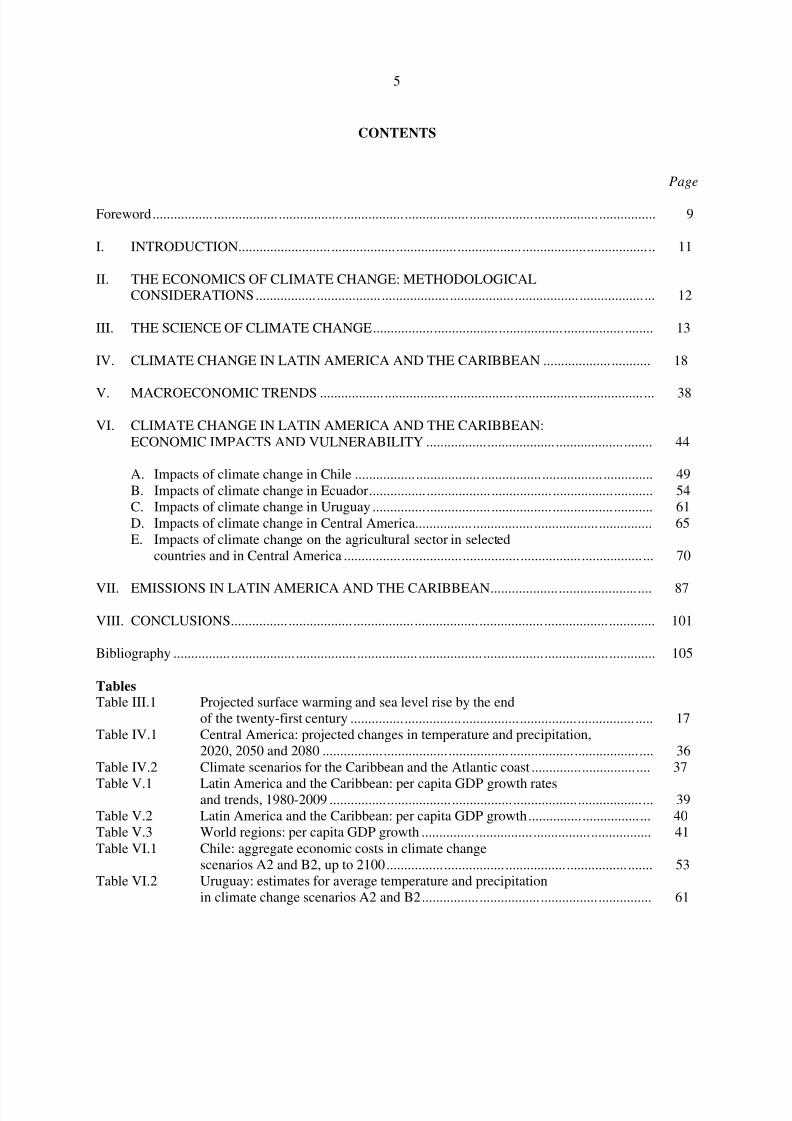
CONTENTS
Page
Foreword ............................................................................................................................................ 9
I. INTRODUCTION.................................................................................................................... 11
II. THE ECONOMICS OF CLIMATE CHANGE: METHODOLOGICALCONSIDERATIONS ............................................................................................................... 12
III. THE SCIENCE OF CLIMATE CHANGE .............................................................................. 13
IV. CLIMATE CHANGE IN LATIN AMERICA AND THE CARIBBEAN .............................. 18
V. MACROECONOMIC TRENDS ............................................................................................. 38
VI. CLIMATE CHANGE IN LATIN AMERICA AND THE CARIBBEAN:ECONOMIC IMPACTS AND VULNERABILITY ............................................................... 44
A. Impacts of climate change in Chile ................................................................................... 49B. Impacts of climate change in Ecuador ............................................................................... 54C. Impacts of climate change in Uruguay .............................................................................. 61D. Impacts of climate change in Central America .................................................................. 65E. Impacts of climate change on the agricultural sector in selected
countries and in Central America ...................................................................................... 70
VII. EMISSIONS IN LATIN AMERICA AND THE CARIBBEAN ............................................. 87
VIII. CONCLUSIONS ...................................................................................................................... 101
Bibliography ...................................................................................................................................... 105
TablesTable III.1 Projected surface warming and sea level rise by the end
of the twenty-first century .................................................................................... 17Table IV.1 Central America: projected changes in temperature and precipitation,
2020, 2050 and 2080 ............................................................................................ 36Table IV.2 Climate scenarios for the Caribbean and the Atlantic coast ................................. 37
Table V.1 Latin America and the Caribbean: per capita GDP growth ratesand trends, 1980-2009 .......................................................................................... 39
Table V.2 Latin America and the Caribbean: per capita GDP growth .................................. 40Table V.3 World regions: per capita GDP growth ................................................................ 41Table VI.1 Chile: aggregate economic costs in climate change
scenarios A2 and B2, up to 2100 .......................................................................... 53Table VI.2 Uruguay: estimates for average temperature and precipitation
in climate change scenarios A2 and B2 ................................................................ 61
8/8/2019 CEPAL Climate Change 2010
http://slidepdf.com/reader/full/cepal-climate-change-2010 6/107
6
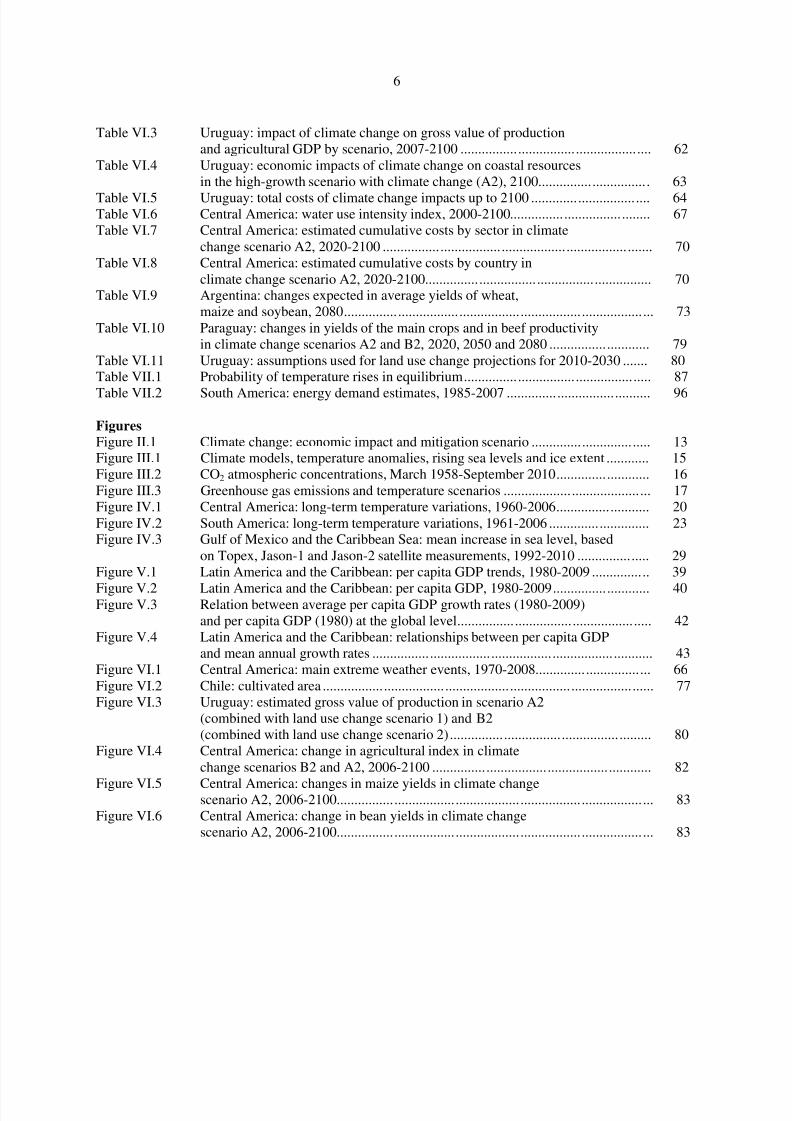
Table VI.3 Uruguay: impact of climate change on gross value of productionand agricultural GDP by scenario, 2007-2100 ..................................................... 62
Table VI.4 Uruguay: economic impacts of climate change on coastal resourcesin the high-growth scenario with climate change (A2), 2100 ............................... 63
Table VI.5 Uruguay: total costs of climate change impacts up to 2100 ................................. 64Table VI.6 Central America: water use intensity index, 2000-2100 ....................................... 67Table VI.7 Central America: estimated cumulative costs by sector in climate
change scenario A2, 2020-2100 ........................................................................... 70Table VI.8 Central America: estimated cumulative costs by country in
climate change scenario A2, 2020-2100 ............................................................... 70Table VI.9 Argentina: changes expected in average yields of wheat,
maize and soybean, 2080 ...................................................................................... 73Table VI.10 Paraguay: changes in yields of the main crops and in beef productivity
in climate change scenarios A2 and B2, 2020, 2050 and 2080 ............................ 79Table VI.11 Uruguay: assumptions used for land use change projections for 2010-2030 ....... 80Table VII.1 Probability of temperature rises in equilibrium .................................................... 87
Table VII.2 South America: energy demand estimates, 1985-2007 ........................................ 96
FiguresFigure II.1 Climate change: economic impact and mitigation scenario ................................. 13Figure III.1 Climate models, temperature anomalies, rising sea levels and ice extent ............ 15Figure III.2 CO2 atmospheric concentrations, March 1958-September 2010 .......................... 16Figure III.3 Greenhouse gas emissions and temperature scenarios ......................................... 17Figure IV.1 Central America: long-term temperature variations, 1960-2006 .......................... 20Figure IV.2 South America: long-term temperature variations, 1961-2006 ............................ 23Figure IV.3 Gulf of Mexico and the Caribbean Sea: mean increase in sea level, based
on Topex, Jason-1 and Jason-2 satellite measurements, 1992-2010 .................... 29Figure V.1 Latin America and the Caribbean: per capita GDP trends, 1980-2009 ................ 39
Figure V.2 Latin America and the Caribbean: per capita GDP, 1980-2009 ........................... 40Figure V.3 Relation between average per capita GDP growth rates (1980-2009)
and per capita GDP (1980) at the global level ...................................................... 42Figure V.4 Latin America and the Caribbean: relationships between per capita GDP
and mean annual growth rates .............................................................................. 43Figure VI.1 Central America: main extreme weather events, 1970-2008 ................................ 66Figure VI.2 Chile: cultivated area ............................................................................................ 77Figure VI.3 Uruguay: estimated gross value of production in scenario A2
(combined with land use change scenario 1) and B2(combined with land use change scenario 2) ........................................................ 80
Figure VI.4 Central America: change in agricultural index in climatechange scenarios B2 and A2, 2006-2100 ............................................................. 82
Figure VI.5 Central America: changes in maize yields in climate changescenario A2, 2006-2100 ........................................................................................ 83
Figure VI.6 Central America: change in bean yields in climate changescenario A2, 2006-2100 ........................................................................................ 83

8/8/2019 CEPAL Climate Change 2010
http://slidepdf.com/reader/full/cepal-climate-change-2010 7/107
7
Figure VI.7 Central America: change in rice yields in climate changescenario A2, 2006-2100 ........................................................................................ 84
Figure VII.1 Aggregate greenhouse gas emissions ................................................................... 88Figure VII.2 Latin America and the Caribbean: aggregate greenhouse gas emissions ............. 89
Figure VII.3 Greenhouse gas emissions, by sector, 2005 .......................................................... 91Figure VII.4 Per capita greenhouse gas emissions, 1990-2005 ................................................. 92Figure VII.5 Latin America and the Caribbean: CO2 emissions from energy
consumption and cement production, 2005 .......................................................... 92Figure VII.6 Latin America and the Caribbean: energy consumption, 1990-2007 ................... 94Figure VII.7 Energy use matrix ................................................................................................. 94Figure VII.8 Latin America and the Caribbean: energy matrix, 2007 ....................................... 95Figure VII.9 Latin America and the Caribbean: per capita energy consumption
and GDP, 2007 ..................................................................................................... 97Figure VII.10 Latin America and the Caribbean: per capita GDP and per capita
energy consumption, 2007 .................................................................................... 97Figure VII.11 Per capita GDP and energy intensity, 2007 .......................................................... 98
Figure VII.12 Latin America and the Caribbean: average annual increase in CO2 emissions and associated factors, 1990-2005 ....................................................... 99
Figure VII.13 Distribution of energy intensity and carbon intensitygrowth rates, 1990-2005 ....................................................................................... 100
MapsMap IV.1 Latin America: rising temperatures and drought .................................................. 19Map IV.2 South America: temperature projections .............................................................. 30Map IV.3 South America: precipitation projections ............................................................. 31Map IV.4 Latin America and the Caribbean: spatial patterns of extreme weather
events under the A1B scenario, based on multi-model averages ......................... 33Map IV.5 Latin America and the Caribbean: overview of projected patterns of
climate change up to 2100 .................................................................................... 34Map IV.6 Central America: climatology of mean temperatures for January, April,
July and October, 1950-2000 ................................................................................ 35Map IV.7 Central America: climatology of precipitation, January, April, July
and October, 1950-2000 ....................................................................................... 36Map VI.1 Latin America and the Caribbean: climate change hot spots ................................ 44Map VI.2 Chile: projected temperature changes in climate change
scenario A2, 2010-2099 ........................................................................................ 50Map VI.3 Chile: projected precipitation changes in climate change
scenario A2, 2010-2099 ........................................................................................ 51Map VI.4 Chile: changes in net revenues of the forestry and crop and livestock
farming sector in climate change scenario A2, 2010-2100 .................................. 52
Map VI.5 Chile: diagram of climate change impacts and their relationswith climate projections ........................................................................................ 54
Map VI.6 Ecuador: change in average temperature with respect to thebaseline in scenario A2, 2100 ............................................................................... 55
Map VI.7 Ecuador: change in precipitation with respect to thebaseline in scenario A2, 2100 ............................................................................... 56
Map VI.8 Ecuador: plant formations in protected natural areas ........................................... 58Map VI.9 Ecuador: increased risk of malaria in rural areas owing to
higher temperatures, 2009-2100 ........................................................................... 59
8/8/2019 CEPAL Climate Change 2010
http://slidepdf.com/reader/full/cepal-climate-change-2010 8/107
8
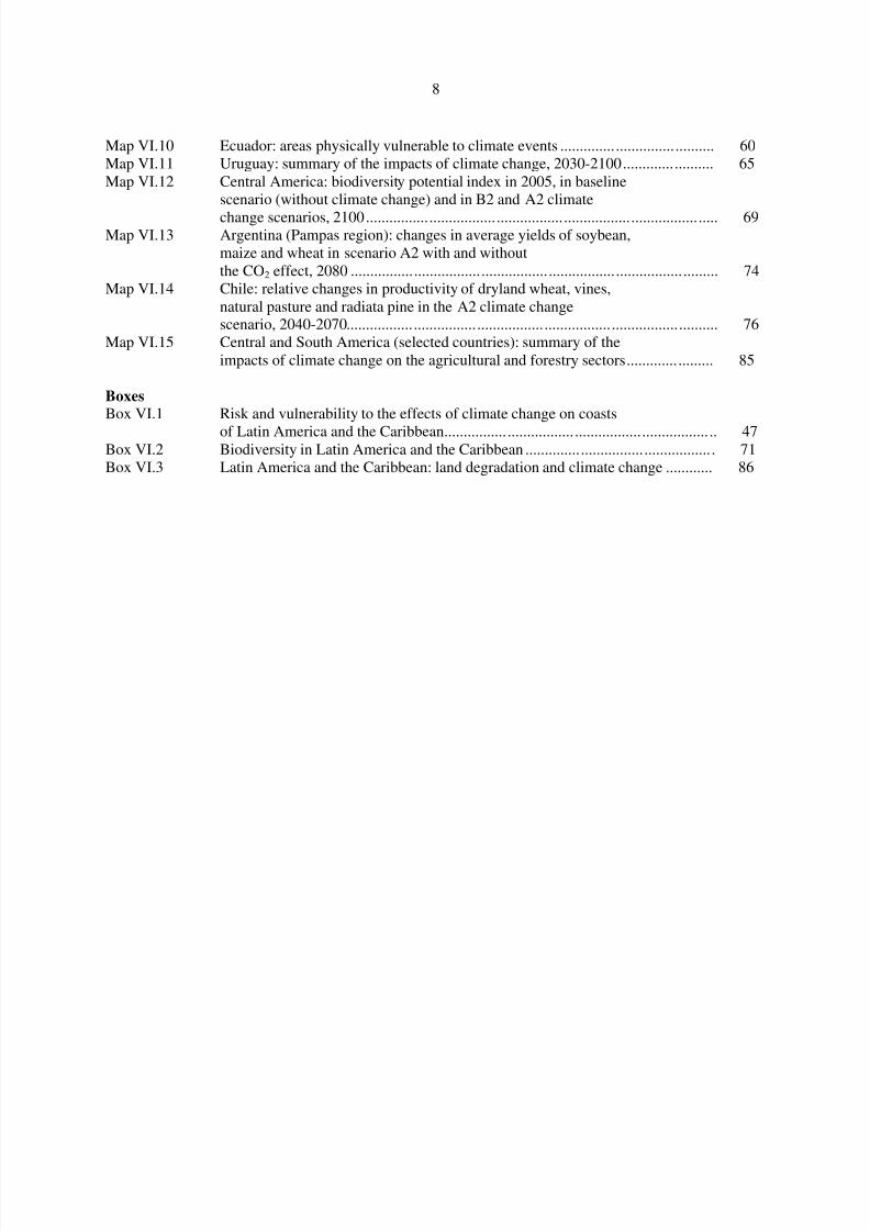
Map VI.10 Ecuador: areas physically vulnerable to climate events ....................................... 60Map VI.11 Uruguay: summary of the impacts of climate change, 2030-2100 ....................... 65Map VI.12 Central America: biodiversity potential index in 2005, in baseline
scenario (without climate change) and in B2 and A2 climate
change scenarios, 2100 ......................................................................................... 69Map VI.13 Argentina (Pampas region): changes in average yields of soybean,
maize and wheat in scenario A2 with and withoutthe CO2 effect, 2080 ............................................................................................. 74
Map VI.14 Chile: relative changes in productivity of dryland wheat, vines,natural pasture and radiata pine in the A2 climate changescenario, 2040-2070 .............................................................................................. 76
Map VI.15 Central and South America (selected countries): summary of theimpacts of climate change on the agricultural and forestry sectors ...................... 85
BoxesBox VI.1 Risk and vulnerability to the effects of climate change on coasts
of Latin America and the Caribbean ..................................................................... 47Box VI.2 Biodiversity in Latin America and the Caribbean ................................................ 71Box VI.3 Latin America and the Caribbean: land degradation and climate change ............ 86

8/8/2019 CEPAL Climate Change 2010
http://slidepdf.com/reader/full/cepal-climate-change-2010 9/107
9
FOREWORD
Climate change, which is basically manifested in rising average temperatures, changes in precipitation
patterns, rising sea levels, reduction of the ice extent, glacier melt and alterations in the pattern of extremeevents, is one of the major challenges facing humankind this century. The evidence available shows thatthese climate transformations are a global phenomenon resulting, above all, from emissions of greenhousegases generated by human activity. In turn, they are having substantial, increasing and in many casesirreversible effects on economic activities, populations and ecosystems, three areas in which the LatinAmerican and Caribbean region is particularly sensitive to climate conditions.
The challenge of adapting to the new climate conditions by cushioning the most negative effectswhile simultaneously participating in an international mitigation strategy, with common but differentiatedresponsibilities, entails economic costs and resources of such a magnitude that climate change willheavily condition the region’s economic development options and characteristics over this century. Thisbeing so, economic analysis of climate change in Latin America is vital not only to identify the main
transmission channels, the scale of climatic effects and the best ways of adapting to the new climateconditions, but also to formulate a long-term sustainable development strategy that combines a low-carbon pathway with social inclusiveness. This is one of the great challenges for the twenty-first century.
This document offers a summary of the aggregate economic analysis of climate change in LatinAmerica and the Caribbean, which was carried out on the basis of national and sectoral studies of climatechange economics in the region. The conclusions are still preliminary, but they offer importantconsiderations regarding the implications of climate change for the region’s countries, with a view toenhancing understanding of the economic dimension of climate change and contributing to the search forpossible solutions.
This study was carried out in close collaboration with the Governments of countries in the region
as well as Governments of Denmark, Germany, Spain and the United Kingdom, the European Union, theInter-American Development Bank (IDB), the Global Mechanism of the United Nations Convention toCombat Desertification and an extensive network of academic and research institutions. The EconomicCommission for Latin America and the Caribbean (ECLAC) remains firm in its commitment to pursuingthis research further and developing the knowledge and awareness needed to give all actors theopportunity to make decisions on the basis of better and fuller information about the different aspects of climate change.
Alicia BárcenaExecutive Secretary
Economic Commission for LatinAmerica and the Caribbean (ECLAC)

8/8/2019 CEPAL Climate Change 2010
http://slidepdf.com/reader/full/cepal-climate-change-2010 10/107

8/8/2019 CEPAL Climate Change 2010
http://slidepdf.com/reader/full/cepal-climate-change-2010 11/107
11
I. INTRODUCTION
Climate change is one of the greatest challenges facing humankind in the twenty-first century. In recent
years, it has attracted an unprecedented degree of public attention, and this has spurred an internationaleffort to reach agreement on mitigation measures and to boost technological innovation and efficiencygains in order to make the transition to low-carbon development paths. It has also prompted seriousconcern about the negative implications that climate change can have for economic and socialdevelopment. Together with the Millennium Development Goals, climate change is at the top of theagenda for the Secretary-General of the United Nations.
The increase in greenhouse gases (GHGs), which is fundamentally linked to various forms of human activity, is clearly bringing about changes in the climate, including gradual but unremittingincreases in temperature, alterations in precipitation patterns, the shrinkage of the cryosphere, rising sealevels and changes in the intensity and frequency of extreme weather events (IPCC, 2007a). Theimplications of climate change for economic activity, the world’s population and its ecosystems are
clearly significant. Moreover, they will increase over the course of the century and, in many cases, areunlikely to be reversed (IPCC, 2007b; Stern, 2007; ECLAC, 2009b). The efforts that will have to be madeto adapt to new climatic conditions while at the same time curbing GHG emissions in order to stabilizeclimate change will entail economic costs and substantive alterations in current production, distributionand consumption patterns, in international financial and trade flows, and in people’s lifestyles. Climatechange will play a key role in shaping the economic development process and development options in thiscentury. This is particularly true for Latin America and the Caribbean, where geographic and climateconditions, vulnerability to extreme weather events, and economic, social and even institutional factorsaccentuate the impact of climate change. The magnitude of the task calls for the formulation of a long-term strategy backed by sound science and a broad social consensus.
An analysis of the economics of climate change provides essential inputs for the identification
and development of strategies to help countries find solutions for the problems associated with climatechange and to attain sustainable development. This kind of analysis is very complex, however, because itencompasses natural, economic, social, technological, environmental and energy-related processes, aswell as certain aspects of international politics. It also deals with very long time frames and has to takeinto account planet-wide natural phenomena, non-linear impacts, specific limits, asymmetric causes andeffects, intense feedback loops, high levels of uncertainty and complex risk management issues, togetherwith significant ethical considerations. Two fundamental aspects of any analysis of the economics of climate change should be borne in mind are:
• The uncertainty margins are considerable, since such analyses must take into account thecomplex risk-management process associated with potentially catastrophic weather events.The projections based on analyses of this type are thus no more than scenarios that have a
certain probability of occurring; they are not specific forecasts. There is also an ethicalcomponent, since the relevant considerations include the well-being of future generations andmatters that have no explicit market value, such as biodiversity and human life.
• The formulation of proposals and strategies for solving problems stemming from climatechange should not be seen as an effort that runs counter to economic growth. On the contrary,it is a failure to address the issue that will have a negative impact on economic growth.Tackling the problems brought about by climate change will entail redirecting the economytowards a low-carbon growth path that is compatible with sustainable economic development.
8/8/2019 CEPAL Climate Change 2010
http://slidepdf.com/reader/full/cepal-climate-change-2010 12/107
12
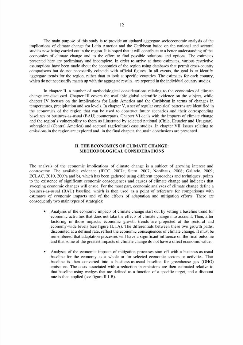
The main purpose of this study is to provide an updated aggregate socioeconomic analysis of theimplications of climate change for Latin America and the Caribbean based on the national and sectoralstudies now being carried out in the region. It is hoped that it will contribute to a better understanding of theeconomics of climate change and to the effort to find possible solutions and options. The estimates
presented here are preliminary and incomplete. In order to arrive at those estimates, various restrictiveassumptions have been made about the economies of the region using databases that permit cross-countrycomparisons but do not necessarily coincide with official figures. In all events, the goal is to identifyaggregate trends for the region, rather than to look at specific countries. The estimates for each country,which do not necessarily match up with the aggregate results, are reported in the individual country studies.
In chapter II, a number of methodological considerations relating to the economics of climatechange are discussed. Chapter III covers the available global scientific evidence on the subject, whilechapter IV focuses on the implications for Latin America and the Caribbean in terms of changes intemperatures, precipitation and sea levels. In chapter V, a set of regular empirical patterns are identified inthe economies of the region that can be used to construct future scenarios and their correspondingbaselines or business-as-usual (BAU) counterparts. Chapter VI deals with the impacts of climate change
and the region’s vulnerability to them as illustrated by selected national (Chile, Ecuador and Uruguay),subregional (Central America) and sectoral (agriculture) case studies. In chapter VII, issues relating toemissions in the region are explored and, in the final chapter, the main conclusions are presented.
II. THE ECONOMICS OF CLIMATE CHANGE:
METHODOLOGICAL CONSIDERATIONS
The analysis of the economic implications of climate change is a subject of growing interest andcontroversy. The available evidence (IPCC, 2007a; Stern, 2007; Nordhaus, 2008; Galindo, 2009;ECLAC, 2010, 2009a and b), which has been gathered using different approaches and techniques, points
to the existence of significant economic consequences and causes of climate change and indicates thatsweeping economic changes will ensue. For the most part, economic analyses of climate change define abusiness-as-usual (BAU) baseline, which is then used as a point of reference for comparisons withestimates of economic impacts and of the effects of adaptation and mitigation efforts. There areconsequently two main types of strategies:
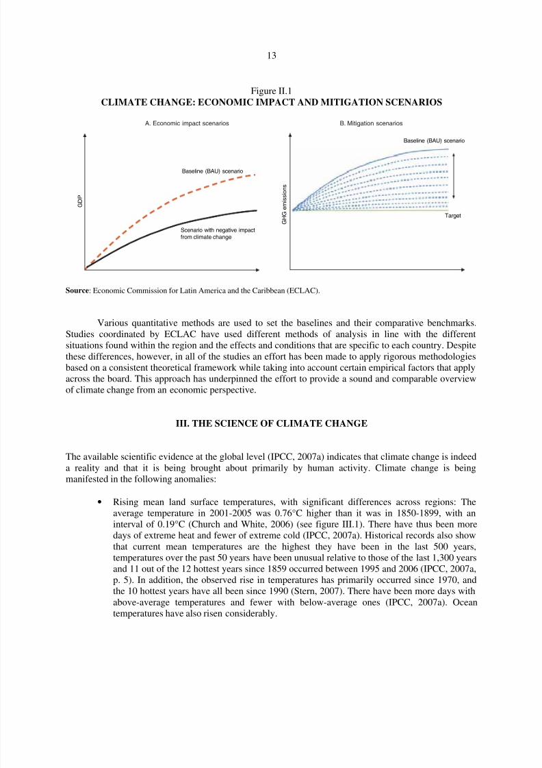
• Analyses of the economic impacts of climate change start out by setting a baseline trend foreconomic activities that does not take the effects of climate change into account. Then, afterfactoring in those impacts, economic growth trends are projected at the sectoral andeconomy-wide levels (see figure II.1.A). The differentials between these two growth paths,discounted at a defined rate, reflect the economic consequences of climate change. It must beremembered that adaptation processes will have a significant influence on the final outcome
and that some of the greatest impacts of climate change do not have a direct economic value.
• Analyses of the economic impacts of mitigation processes start off with a business-as-usualbaseline for the economy as a whole or for selected economic sectors or activities. Thatbaseline is then converted into a business-as-usual baseline for greenhouse gas (GHG)emissions. The costs associated with a reduction in emissions are then estimated relative tothat baseline using wedges that are defined as a function of a specific target, and a discountrate is then applied (see figure II.1.B).
8/8/2019 CEPAL Climate Change 2010
http://slidepdf.com/reader/full/cepal-climate-change-2010 13/107
13
Figure II.1CLIMATE CHANGE: ECONOMIC IMPACT AND MITIGATION SCENARIOS
Source: Economic Commission for Latin America and the Caribbean (ECLAC).
Various quantitative methods are used to set the baselines and their comparative benchmarks.Studies coordinated by ECLAC have used different methods of analysis in line with the differentsituations found within the region and the effects and conditions that are specific to each country. Despitethese differences, however, in all of the studies an effort has been made to apply rigorous methodologiesbased on a consistent theoretical framework while taking into account certain empirical factors that applyacross the board. This approach has underpinned the effort to provide a sound and comparable overviewof climate change from an economic perspective.
III. THE SCIENCE OF CLIMATE CHANGE
The available scientific evidence at the global level (IPCC, 2007a) indicates that climate change is indeeda reality and that it is being brought about primarily by human activity. Climate change is beingmanifested in the following anomalies:
• Rising mean land surface temperatures, with significant differences across regions: Theaverage temperature in 2001-2005 was 0.76°C higher than it was in 1850-1899, with aninterval of 0.19°C (Church and White, 2006) (see figure III.1). There have thus been more
days of extreme heat and fewer of extreme cold (IPCC, 2007a). Historical records also showthat current mean temperatures are the highest they have been in the last 500 years,temperatures over the past 50 years have been unusual relative to those of the last 1,300 yearsand 11 out of the 12 hottest years since 1859 occurred between 1995 and 2006 (IPCC, 2007a,p. 5). In addition, the observed rise in temperatures has primarily occurred since 1970, andthe 10 hottest years have all been since 1990 (Stern, 2007). There have been more days withabove-average temperatures and fewer with below-average ones (IPCC, 2007a). Oceantemperatures have also risen considerably.
G D P
G H G
e m i s s i o n s
A. Economic impact scenarios B. Mitigation scenarios
Baseline (BAU) scenario
Scenario with negative impact
from climate change
Target
Baseline (BAU) scenario
8/8/2019 CEPAL Climate Change 2010
http://slidepdf.com/reader/full/cepal-climate-change-2010 14/107
14
• Changing precipitation patterns, with significant differences across regions: It is raining morein high-precipitation areas and less in arid regions, which is resulting in more flooding andmore droughts (IPCC, 2007a). There is also a cause-and-effect cycle of higher temperatures andlower precipitation that triggers more extreme weather events (Madden and Williams, 1978).
• Rising sea levels: Sea level rose between 1.3 and 2.3 mm, with an average annual increase of 1.8 mm, between 1961 and 2003, while the increase was between 2.4 and 3.8 mm, with anannual average of 3.1 mm, for 1993-2003 (IPCC, 2007a) (see figure III.1). The melting of glaciers and the polar ice caps is one of the contributing factors.
• Shrinkage of the cryosphere: Since 1978, the ice cap has retreated by 2.7% per decade, andthe reduction is as much as 7.4% during the summer (IPCC, 2007a) (see figure III.1). InSeptember 2010, the average surface area of the ice sheet was 4.9 million square kilometres,which was 2.14 million square kilometres less than the average for 1979-2000 (NSIDC,2010). The size and number of glacial lakes has also increased (Polyak and others, 2010),while glaciers have shrunk significantly.
• Changes in the types, intensity and frequency of extreme weather events: Rising temperaturesheighten the probability of changes in the frequency and intensity of extreme events (e.g., theincrease in cyclonic activity in the North Atlantic) (Vincent and others, 2005; Aguilar andothers, 2005; Kiktev and others, 2003; IPCC, 2007a, p. 300; Marengo and others, 2009a and b).
The available evidence thus indicates that these climate changes can be properly modelled only if the natural and anthropogenic forcings associated with greenhouse gas (GHG) emissions is taken intoaccount (IPCC, 2007a). GHG emissions arise from natural processes as well as anthropogenic activitiessuch as the use of fossil fuels, industrial processes (e.g., cement production), agriculture, deforestationand land-use changes (IPCC, 2007a; Stern, 2007).1
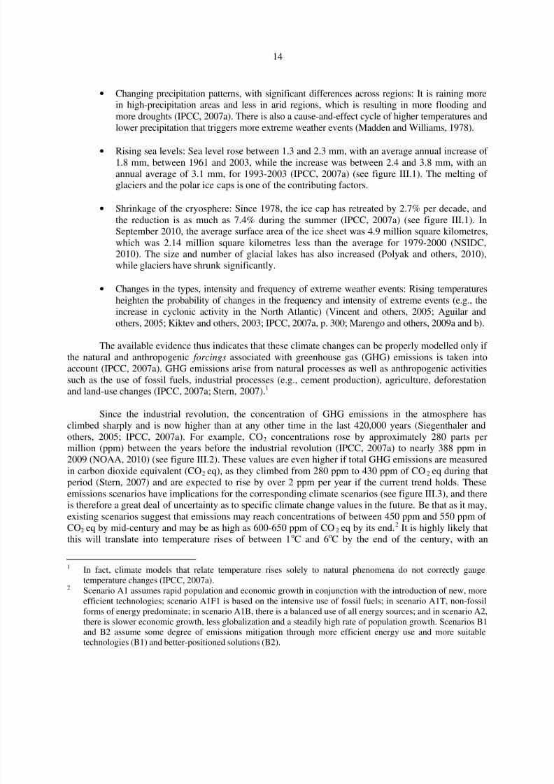
Since the industrial revolution, the concentration of GHG emissions in the atmosphere hasclimbed sharply and is now higher than at any other time in the last 420,000 years (Siegenthaler andothers, 2005; IPCC, 2007a). For example, CO2 concentrations rose by approximately 280 parts permillion (ppm) between the years before the industrial revolution (IPCC, 2007a) to nearly 388 ppm in2009 (NOAA, 2010) (see figure III.2). These values are even higher if total GHG emissions are measuredin carbon dioxide equivalent (CO2 eq), as they climbed from 280 ppm to 430 ppm of CO 2 eq during thatperiod (Stern, 2007) and are expected to rise by over 2 ppm per year if the current trend holds. Theseemissions scenarios have implications for the corresponding climate scenarios (see figure III.3), and thereis therefore a great deal of uncertainty as to specific climate change values in the future. Be that as it may,existing scenarios suggest that emissions may reach concentrations of between 450 ppm and 550 ppm of CO2 eq by mid-century and may be as high as 600-650 ppm of CO 2 eq by its end.2 It is highly likely thatthis will translate into temperature rises of between 1oC and 6oC by the end of the century, with an
1 In fact, climate models that relate temperature rises solely to natural phenomena do not correctly gaugetemperature changes (IPCC, 2007a).
2 Scenario A1 assumes rapid population and economic growth in conjunction with the introduction of new, moreefficient technologies; scenario A1F1 is based on the intensive use of fossil fuels; in scenario A1T, non-fossilforms of energy predominate; in scenario A1B, there is a balanced use of all energy sources; and in scenario A2,there is slower economic growth, less globalization and a steadily high rate of population growth. Scenarios B1and B2 assume some degree of emissions mitigation through more efficient energy use and more suitabletechnologies (B1) and better-positioned solutions (B2).

8/8/2019 CEPAL Climate Change 2010
http://slidepdf.com/reader/full/cepal-climate-change-2010 15/107
15
average of between approximately 2oC and 4oC (see table III.1). These high emissions scenarios alsopoint to feedback effects that are difficult to model and that will very likely lead to more intense and morefrequent changes in weather patterns (IPCC, 2007a). In addition, sea levels are expected to rise bybetween 18 and 59 centimetres (see table III.1), while other weather phenomena, such as changes in
global precipitation patterns, the shrinkage of the cryosphere, the retreat of the glaciers and the increase inthe number and intensity of extreme weather events, are expected to intensify (IPCC, 2007a).3
Figure III.1CLIMATE MODELS, TEMPERATURE ANOMALIES, RISING SEA LEVELS AND ICE EXTENT
Source: Intergovernmental Panel on Climate Change (IPCC), Climate Change 2007 - The Physical Science Basis. Contributionof Working Group I to the Fourth Assessment Report of the Intergovernmental Panel on Climate Change, CambridgeUniversity Press, 2007; and Economic Commission for Latin America and the Caribbean (ECLAC), on the basis of information from the National Oceanic and Atmospheric Administration (NOAA) and the National Snow and Ice DataCenter (NSIDC) of the United Sates.
a The data on altimetry came from the Laboratory for Satellite Altimetry del NOAA [on line] http://ibis.grdl.noaa.gov/ SAT/slr/LSA_SLR_timeseries_global.php. The effects of seasonal variations have been eliminated. Six-month moving averages.
3 The projections of rising sea levels prepared by IPCC (2007a) are acknowledged to be highly uncertain. The globalscenarios for average temperature ranges relative to increases in sea level differ sharply, and studies have thereforebeen undertaken in an effort to resolve the question through the use of various semi-empirical approaches (simplestatistical models relating the rise in the planet’s average temperature to rising sea levels). Vermeer andRahnmstorf (2009) have carried out studies which indicate that, by 2100, the average sea level, planet-wide, willhave risen by about one metre, which is higher than the IPCC (2007a) estimate for the same period.
−30
−20
−10
0
10
20
30
*********
******
****************************************
********************************
****************
*****************************
**********************
*******************************************
***********************
**********************
*******************************
**********************************
1992 1994 1996 1998 2000 2002 2004 2006 2008 2010
TOPEX
Jason−1
Jason−2
1980 1985 1990 1995 2000 2005 2010
4.5
5.0
5.5
6.0
6.5
7.0
7.5
8.0
Temperature changes, by climatological model
(degrees Centigrade)
Modelled using natural plus anthropogenic forcings
Modelled using natural forcings only
World Land (global) Oceans (global)
Año
Año
Año
Año
Año
Año
Año Año Año
Observations
T e m p e r a t u r e a n o m a l y ( o C )
T e m p e r a t u r e a n o m a l y ( o C )
T e m p e r a t u r e a n o m a l y ( o C )
T e m p e r a t u r e a n o m a l y ( o C )
T e m p e r a t u r e a n o m a l y ( o C )
T e m p e r a t u r e a n o m a l y ( o C )
T e
m p e r a t u r e a n o m a l y ( o C )
T e m p e r a t u r e a n o m a l y ( o C )
T e m p e r a t u r e a n o m a l y ( o C )
1.0
0.5
0.0
1.0
0.5
0.0
1.0
0.5
0.0
1.0
0.5
0.0
1.0
0.5
0.0
1.0
0.5
0.0
1.0
0.5
0.0
1.0
0.5
0.0
1.0
0.5
0.0
1880 1900 1920 1940 1960 1980 2000
−0.4
−0.2
0.0
0.2
0.4
0.6
Global temperature anomalies
(base: 1901-2000)
Average rise in sea level TOPEX, Jason-1 and Jason-2 a
satellite measurements
(millimetres)
Average minimum extent of the Arctic ice pack
(millions of square metres)
North America
South America
Africa
Europe
Asia
Australia
●
●
●
● ●
●
●
● ● ●
●
●
●
●
●
●
●
●
●●
● ●
●
●●
●
●
●
●
●
●
●
8/8/2019 CEPAL Climate Change 2010
http://slidepdf.com/reader/full/cepal-climate-change-2010 16/107
16
Figure III.2CO2 ATMOSPHERIC CONCENTRATIONS, MARCH 1958-SEPTEMBER 2010
a
(Parts per million)
Source: Economic Commission for Latin America and the Caribbean (ECLAC), on the basis of information from the NationalOceanic and Atmospheric Administration (NOAA) of the United States.
a Measurements carried out at the Mauna Loa Observatory, Hawaii.
The evidence points to a close correlation between GHG emissions and climate change and helps toidentify a number of factors to be taken into account in economic analyses of the impact of climate change:
• In economic terms, the atmosphere is a public good and, viewed from this standpoint, climatechange is the most serious conceivable externality (Stern, 2007). Its correction may entail theuse of a range of economic instruments, but, given the current sensitivity of responses to the useof such instruments, the importance of proper regulatory oversight must be borne in mind.
• Given the existence of various feedback loops, the fact that the response sensitivity of anumber of factors is unknown and the long-term nature of climate change, a high degree of uncertainty is associated with the long-term scenarios that are being constructed. Thus, theprojections that are being calculated are just that, scenarios, rather than specific predictions
(Clements and Hendry, 2004).
• Climate change may be associated with catastrophic weather events or natural disasters. Risk management for low-probability catastrophic events over a long time horizon is certainly acomplex undertaking. The first-best solutions that may be identified when taking decisionsconcerning investment in the adaptation to and prevention of potentially extreme weatherevents, for example, are a complicated matter that should be looked at as a form of “climatechange insurance”.
1960 1970 1980 1990 2000 2010
310
320
330
340
350
360
370
380
390
Monthly average Seasonally adjusted

8/8/2019 CEPAL Climate Change 2010
http://slidepdf.com/reader/full/cepal-climate-change-2010 17/107
17
Figure III.3
GREENHOUSE GAS EMISSIONS AND TEMPERATURE SCENARIOS(Annual Gt of CO2 eq and Centigrade degrees)
Source: Intergovernmental Panel on Climate Change (IPCC), Climate Change 2007 - The Physical Science Basis. Contributionof Working Group I to the Fourth Assessment Report of the Intergovernmental Panel on Climate Change, CambridgeUniversity Press, 2007.
Table III.1PROJECTED SURFACE WARMING AND SEA LEVEL RISE BY THE END
OF THE TWENTY-FIRST CENTURY
Case
Temperature changes in 2090-2099relative to1980-1999
a
(in degrees Centigrade)
Rise in sea level in 2090-2099 relative
to 1980-1999(in metres)
Best estimate Likely changeModelled intervals, excluding future
changes in ice floes
Constant concentrations as of 2000 b 0.6 0.3-0.9 Not available
Scenario B1 c 1.8 1.1-2.9 0.18-0.38
Scenario A1T c 2.4 1.4-3.8 0.20-0.45
Scenario B2 c 2.4 1.4-3.8 0.20-0.43
Scenario A1B c 2.8 1.7-4.4 0.21-0.48
Scenario A2 c 3.4 2.0-5.4 0.23-0.51
Scenario A1F1c
4.0 2.4-6.4 0.26-0.59
Source: Intergovernmental Panel on Climate Change (IPCC), Climate Change 2007 - The Physical Science Basis. Contribution
of Working Group I to the Fourth Assessment Report of the Intergovernmental Panel on Climate Change, CambridgeUniversity Press, 2007.
a These projections are assessed using a hierarchy of models that encompasses a simple climate model, several earth-systemmodels of intermediate complexity (EMICs) and a large number of atmosphere-ocean general circulation models (AOGCMs).
b The composition at constant year 2000 values is derived solely from AOGCMS.c Scenario A1 assumes rapid population and economic growth in conjunction with the introduction of new, more efficient
technologies; scenario A1F1 is based on the intensive use of fossil fuels; in scenario A1T, non-fossil forms of energypredominate; in scenario A1B, there is a balanced use of all energy sources; and in scenario A2, there is slower economicgrowth, less globalization and a steadily high rate of population growth. Scenarios B1 and B2 assume some degree of emissionsmitigation through more efficient energy use and more suitable technologies (B1) and better-positioned solutions (B2).
B 1
Year
-1
0
1
2
3
5
6
4
1900 2000 2100
Post-SRES range (80%)A1B
B1
A2
A1F1
A1T
B2
Constant year 2000 concentrations
Twentieth century
G l o b a l s u r f a c e w a r m i n g ( ° C )
Year
G l o b a l g r e e n h o u s e g a s e m i s s i o n s ( g t o f C O 2 a y e a r )
200
160
150
140
120
100
60
50
40
20
0
2000 2100
Post-SRES (max.)
Post-SRES (min.) A 1 T B 2
A 1 B A 2
A 1 F 1

8/8/2019 CEPAL Climate Change 2010
http://slidepdf.com/reader/full/cepal-climate-change-2010 18/107
18
IV. CLIMATE CHANGE IN LATIN AMERICA AND THE CARIBBEAN
The available evidence concerning climate change in Latin America and the Caribbean indicates that the
patterns are similar to those seen at the global level.1 The region is experiencing a gradual but steady rise inoverall land temperatures of approximately 0.74°C ± 0.18°C, measured as a linear trend over the past 100years (1906-2005). The trend increase nearly doubles, however, if the frame of reference is restricted to thepast 50 years (0.13°C ± 0.03°C per decade, compared to 0.07°C ± 0.02°C) (Trenberth and others, 2007).Furthermore, between 1970 and 2005, a mean increase of approximately 0.3°C–0.5°C per decade wasobserved in South and Central America, with a sharper rise in northern Mexico and Amazonia (Trenberthand others, 2007). The evidence indicates that temperatures have climbed by about 1°C in Meso-Americaand some parts of South America. In contrast, temperatures have been declining somewhat along thewestern coast of southern Peru and Chile (see map IV.1.A). The level, intensity and frequency of precipitation also changed between 1900 and 2005 (Trenberth and others, 2007). Increased precipitation has,for example, resulted in more frequent and more serious flooding in Paraguay, Uruguay, the Argentinepampas and some regions of the Plurinational State of Bolivia, whereas the north-eastern, north-western and
northern regions of South America have witnessed a decline (see map IV.1.B), as have southern Chile,south-western Argentina, southern Peru and western Central America. Changes in precipitation patterns invarious regions of the Caribbean are also expected. Glaciers in southern Latin America will continue torecede, and this will have an impact on the water supply over the long term. The weather is also becomingincreasingly variable, and this is associated with a mounting number of extreme events, such as those thatoccurred in the Bolivarian Republic of Venezuela in 1999 and 2005 and in the Argentine pampas in 2000-2002, as well as the hail and ice storms that hit the Plurinational State of Bolivia in 2002 and the BuenosAires metropolitan area in 2006, and during the 2005 hurricane season in the Caribbean.
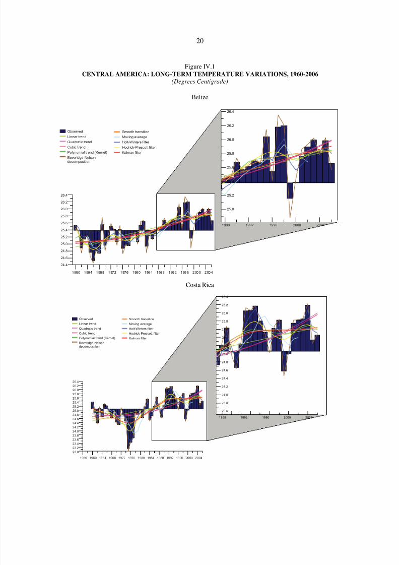
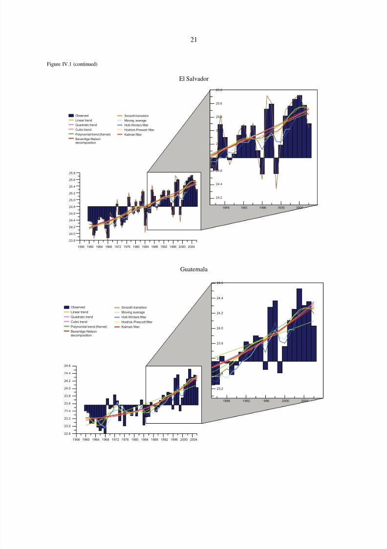
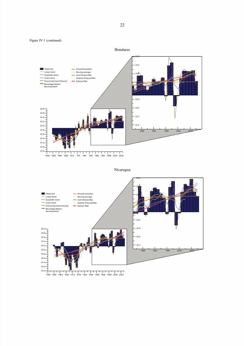
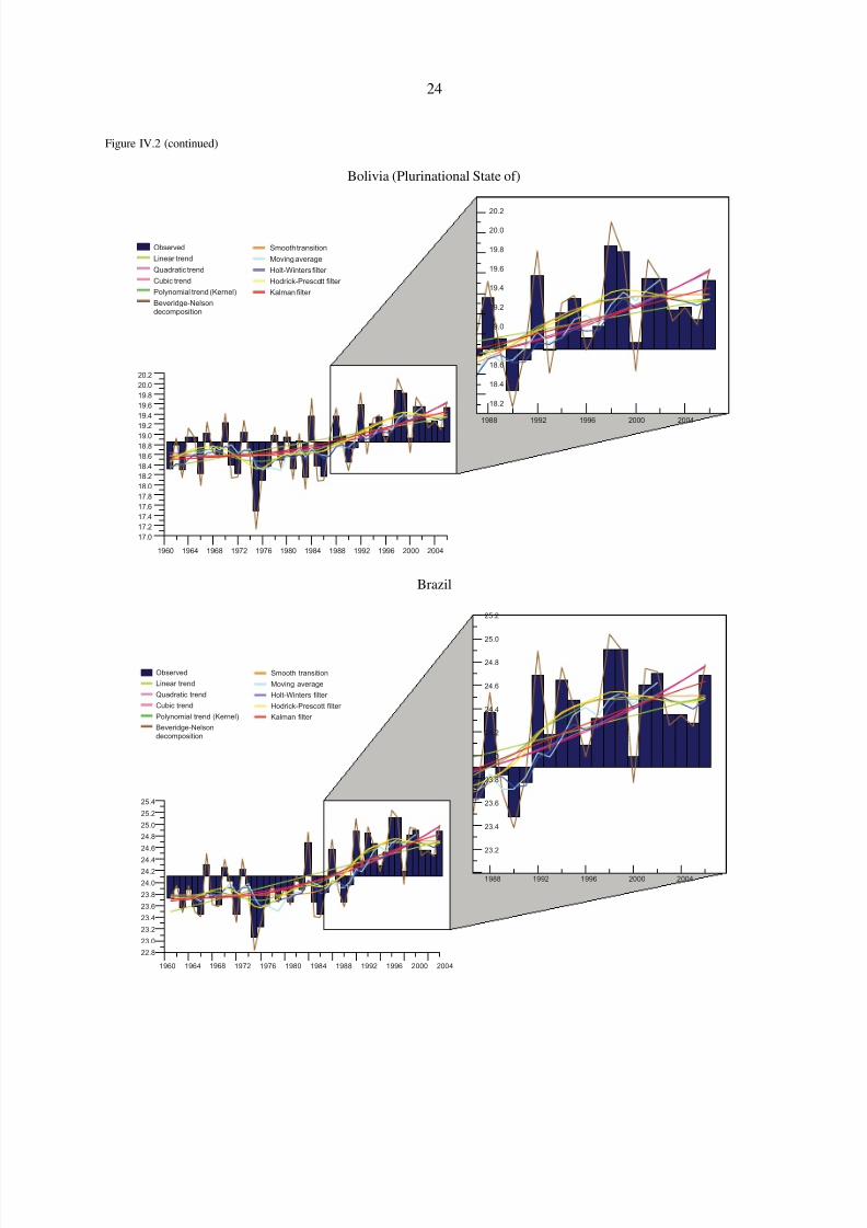
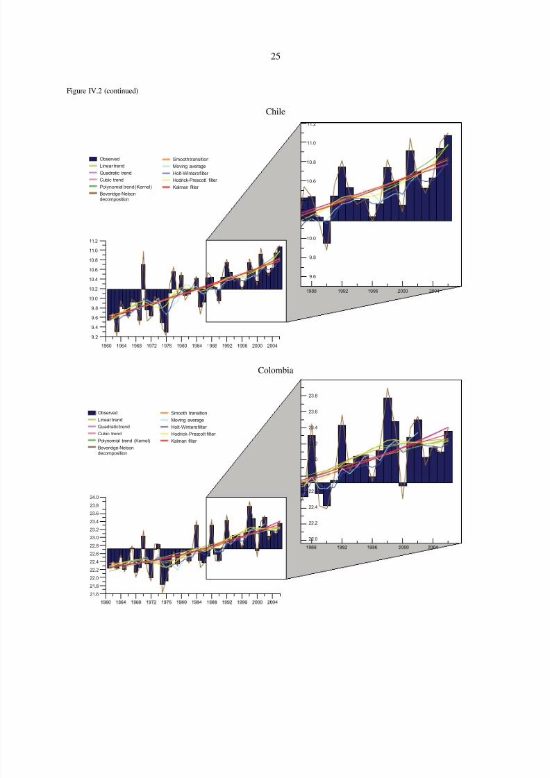
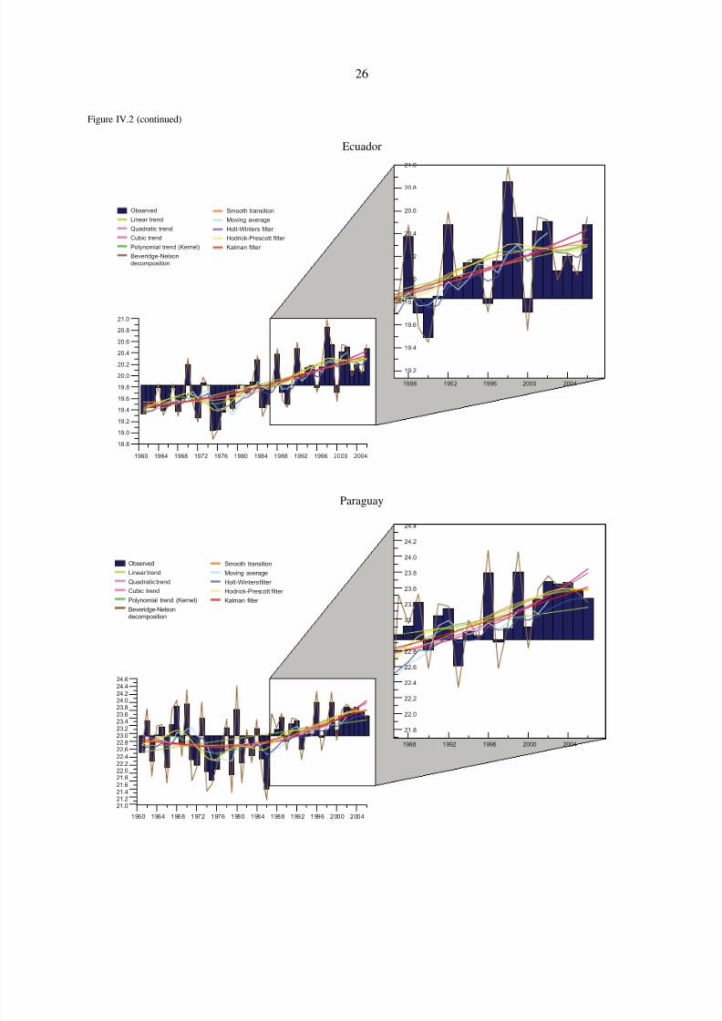
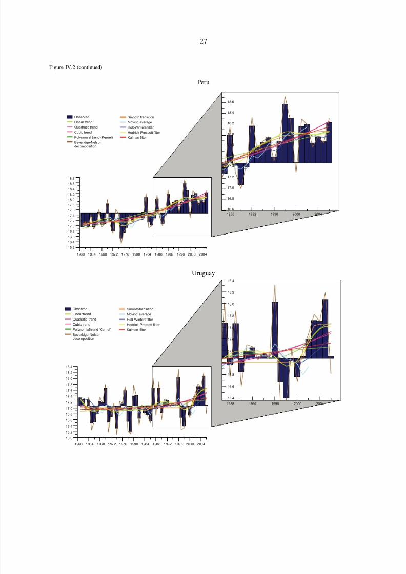
There is solid evidence that temperatures are rising in the individual Central American and SouthAmerican countries, as is demonstrated by the long-run upward trend, although the strength of this trendvaries across countries and the margin of error is significant. Climatic variables, such as temperature and
precipitation, usually follow regular patterns in which they fluctuate around a stochastic or deterministictrend or constant. An analysis of unobservable components can then be undertaken (Maravall, 1999;Mills, 2003; Canova, 2007) in order to determine which components are permanent and which aretransitory,2 with the permanent components represented as a trend or a non-stationary component and thetemporary one represented as a stationary serie.3 The simultaneous application of a broad spectrum of methods for disaggregating the series makes it possible to obtain sound evidence about these regularpatterns and particularly about the presence of an upward trend in temperature. Consequently, the analysisof unobservable components with respect to approximate changes in temperatures at the country levelpoints to the presence of an upward trend, although considerable differences are to be seen across
1 The downscaling of global climate scenarios to the regional level entails an even higher degree of uncertaintythan exists at the global level. A single global scenario generates a variety of probable regional scenarios, andregional scenarios must incorporate a larger number of specific factors relating, for example, to interactionswith different forms of land use or to different elevations (IPCC, 2007a and b).
2 Seasonal patterns have been factored out.3 Various techniques can be used to accomplish this decomposition of unobservable components, although there is
no consensus as to the best way of specifying the model or estimating the values (Maravall, 1999), nor is there anyassurance of consistency in the decomposition. In addition, different trend models generate different cyclicalcomponents and thus pose the risk of generating spurious results (Watson, 1986; Maravall, 1999; Mills, 2003).
8/8/2019 CEPAL Climate Change 2010
http://slidepdf.com/reader/full/cepal-climate-change-2010 19/107
19
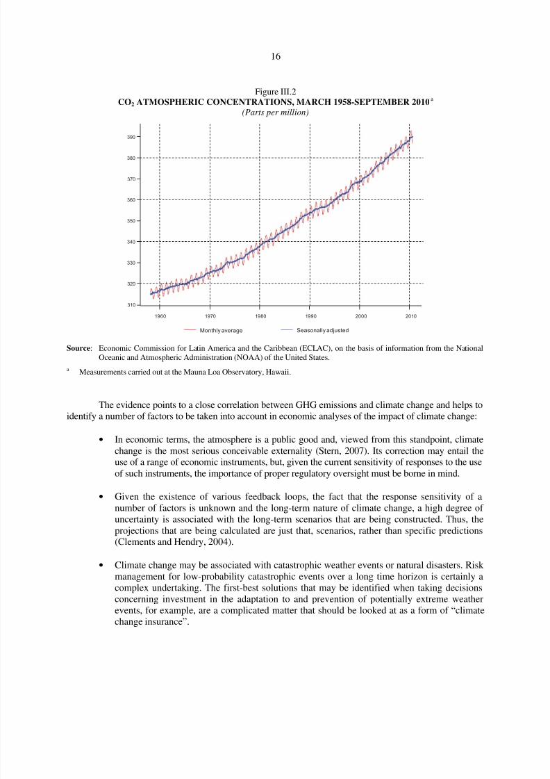
countries (see figures IV.1 and IV.2).4 Unit-root tests have been performed which substantiate this trend(Watson, 1986; Maravall, 1999; Mills, 2003).
Map IV.1LATIN AMERICA: RISING TEMPERATURES AND DROUGHT
Source: K.E. Trenberth and others, “Observations: surface and atmospheric climate change”, Climate Change 2007: ThePhysical Science Basis. Contribution of Working Group I to the Fourth Assessment Report of the IPCC, Cambridge,Cambridge University Press, 2007.
a The grey areas denote those for which there is not enough data to generate reliable trends. The trend for 1979-2005 is calculatedon the basis of 18 annual observations. An annual value is obtained if 10 valid monthly values denoting temperature anomaliesare present. The database used for this purpose was compiled by the National Climatic Data Center (NCDC) on the basis of Smith and Reynolds (2005). Trends with a 5% significance level are marked with a white plus sign (+).
b The positive (blue) and negative (red) values of the index correspond to areas that are wetter or drier than the average.
4 Hodrick-Prescott linear, quadratic and cubic trend filters, Kernel polynomials and Beveridge-Nelsondecomposition, and Holt-Winters and Kalman smooth transition models were applied (Hodrick and Prescott,1997; Maravall, 1999; Mills, 2003; Canova, 2007). Temperature estimates at the country level are difficult tocalculate because they do not correspond to climatic zones and are therefore only approximate.
<-1.3 -1.1 -0.9 -0.7 -0.5 -0.1 0 0.1 0.3 0.5 0.7 0.9 1.1 >1.3 - 4 - 2 0 2 4-0.3
A. Linear trend in annual temperatures, 1979-2005 a
(Degrees Centigrade, per decade)
B. Spatial patterns measured by the Palmer Drought
Severity Index, 1990-2002 b
<-1.3 -1.1 -0.9 -0.7 -0.5 -0.1 0 0.1 0.3 0.5 0.7 0.9 1.1 >1.3 - 4 - 2 0 2 4-0.3
8/8/2019 CEPAL Climate Change 2010
http://slidepdf.com/reader/full/cepal-climate-change-2010 20/107
20
Figure IV.1CENTRAL AMERICA: LONG-TERM TEMPERATURE VARIATIONS, 1960-2006
(Degrees Centigrade)
Belize
Costa Rica
1960 1964 1968 1972 1976 1980 1984 1988 1992 1996 2000 2004
26.4
26.2
26.0
25.8
25.6
25.4
25.2
25.0
24.8
24.6
24.4
1988 1992 1996 2000 2004
26.4
26.2
26.0
25.8
25.6
25.4
25.2
25.0
Observed
Linear trend
Quadratic trend
Cubic trend
Polynomial trend (Kernel)
Beveridge-Nelsondecomposition
Smooth transition
Moving average
Holt-Winters filter
Hodrick-Prescott filter
Kalman filter
26.4
26.2
26.0
25.8
25.6
25.4
25.2
25.0
24.8
24.6
24.4
24.2
24.0
23.8
23.6
23.4
23.2
23.0
1960 1964 1968 1972 1976 1980 1984 1988 1992 1996 2000 20041956
26.4
26.2
26.0
25.8
25.6
25.4
25.2
25.0
24.8
24.6
24.4
24.2
24.0
23.8
23.6
1988 1992 1996 2000 2004
Observed
Linear trend
Quadratic trend
Cubic trend
Polynomial trend (Kernel)
Beveridge-Nelsondecomposition
Smooth transition
Moving average
Holt-Winters filter
Hodrick-Prescott filter
Kalman filter
8/8/2019 CEPAL Climate Change 2010
http://slidepdf.com/reader/full/cepal-climate-change-2010 21/107
21
Figure IV.1 (continued)
El Salvador
Guatemala
25.8
25.6
25.4
25.2
25.0
24.8
24.6
24.4
24.2
24.0
23.8
1956 1960 1964 1968 1972 1976 1980 1984 1988 1992 1996 2000 2004
1988 1992 1996 2000 2004
25.8
25.6
25.4
25.2
25.0
24.8
24.6
24.4
24.2
Observed
Linear trend
Quadratic trend
Cubic trend
Polynomial trend (Kernel)
Beveridge-Nelsondecomposition
Smooth transition
Moving average
Holt-Winters filter
Hodrick-Prescott filter
Kalman filter
24.6
24.4
24.2
24.0
23.8
23.6
23.4
23.2
23.0
22.8
19601956 1964 1968 1972 1976 1980 1984 1988 1992 1996 2000 2004
1988 1992 1996 2000 2004
24.6
24.4
24.2
24.0
23.8
23.6
23.4
23.2
Observed
Linear trend
Quadratic trend
Cubic trend
Polynomial trend (Kernel)
Beveridge-Nelson
decomposition
Smooth transition
Moving average
Holt-Winters filter
Hodrick-Prescott filter
Kalman filter
8/8/2019 CEPAL Climate Change 2010
http://slidepdf.com/reader/full/cepal-climate-change-2010 22/107
22
Figure IV.1 (continued)
Honduras
Nicaragua
24.8
24.6
24.4
24.2
24.0
23.8
23.6
23.4
23.2
23.0
22.8
19601956 1964 1968 1972 1976 1980 1984 1988 1992 1996 2000 2004
24.8
24.6
24.4
24.2
24.0
23.8
23.6
23.4
23.2
1988 1992 1996 2000 2004
Observed
Linear trend
Quadratic trend
Cubic trend
Polynomial trend (Kernel)
Beveridge-Nelsondecomposition
Smooth transition
Moving average
Holt-Winters filter
Hodrick-Prescott filter
Kalman filter
26.0
25.8
25.6
25.4
25.2
25.0
24.8
24.6
24.4
24.2
24.0
19601956 1964 1968 1972 1976 1980 1984 1988 1992 1996 2000 2004
26.0
25.8
25.6
25.4
25.2
25.0
24.8
24.6
24.4
1988 1992 1996 2000 2004
Observed
Linear trend
Quadratic trend
Cubic trend
Polynomial trend (Kernel)
Beveridge-Nelsondecomposition
Smooth transition
Moving average
Holt-Winters filter
Hodrick-Prescott filter
Kalman filter

8/8/2019 CEPAL Climate Change 2010
http://slidepdf.com/reader/full/cepal-climate-change-2010 23/107
23
Figure IV.1 (concluded)
Panama
Source: Economic Commission for Latin America and the Caribbean (ECLAC), on the basis of Global Climate Data(WorldClim) [online database] http://www.worldclim.org
Figure IV.2SOUTH AMERICA: LONG-TERM TEMPERATURE VARIATIONS, 1961-2006
(Degrees Centigrade)
Argentina
26.2
26.0
25.8
25.6
25.4
25.2
25.024.8
24.6
24.4
24.2
24.0
23.8
19601956 1964 1968 1972 1976 1980 1984 1988 1992 1996 2000 2004
1988 1992 1996 2000 2004
26.2
26.0
25.8
25.6
25.4
25.2
25.0
24.8
24.6
24.4
24.2
Observed
Linear trend
Quadratic trend
Cubic trend
Polynomial trend (Kernel)
Beveridge-Nelsondecomposition
Smooth transition
Moving average
Holt-Winters filter
Hodrick-Prescott filter
Kalman filter
17.016.8
16.6
16.4
16.2
16.0
15.8
15.6
15.4
15.2
15.0
14.8
14.6
14.4
1960 1964 1968 1972 1976 1980 1984 1988 1992 1996 2000 2004
1988 1992 1996 2000 2004
17.0
16.8
16.6
16.4
16.2
16.0
15.8
15.6
15.4
15.2
15.0
14.8
14.6
Observed
Linear trend
Quadratic trend
Cubic trend
Polynomial trend (Kernel)
Beveridge-Nelsondecomposition
Smooth transition
Moving average
Holt-Winters filter
Hodrick-Prescott filter
Kalman filter
8/8/2019 CEPAL Climate Change 2010
http://slidepdf.com/reader/full/cepal-climate-change-2010 24/107
24
Figure IV.2 (continued)
Bolivia (Plurinational State of)
Brazil
20.2
20.0
19.8
19.6
19.4
19.2
19.0
18.8
18.6
18.4
18.2
18.0
17.8
17.6
17.4
17.2
17.0
1960 1964 1968 1972 1976 1980 1984 1988 1992 1996 2000 2004
1988 1992 1996 2000 2004
20.2
20.0
19.8
19.6
19.4
19.2
19.0
18.8
18.6
18.4
18.2
Observed
Linear trend
Quadratic trend
Cubic trend
Polynomial trend (Kernel)
Beveridge-Nelsondecomposition
Smooth transition
Moving average
Holt-Winters filter
Hodrick-Prescott filter
Kalman filter
25.4
25.2
25.0
24.8
24.6
24.424.2
24.0
23.8
23.6
23.4
23.2
23.0
22.8
1988 1992 1996 2000 2004
1960 1964 1968 1972 1976 1980 1984 1988 1992 1996 2000 2004
25.2
25.0
24.8
24.6
24.4
24.2
24.0
23.8
23.6
23.4
23.2
Observed
Linear trend
Quadratic trend
Cubic trend
Polynomial trend (Kernel)
Beveridge-Nelson
decomposition
Smooth transition
Moving average
Holt-Winters filter
Hodrick-Prescott filter
Kalman filter
8/8/2019 CEPAL Climate Change 2010
http://slidepdf.com/reader/full/cepal-climate-change-2010 25/107
25
Figure IV.2 (continued)
Chile
Colombia
11.2
11.0
10.8
10.6
10.4
10.2
10.0
9.8
9.6
9.4
9.2
1960 1964 1968 1972 1976 1980 1984 1988 1992 1996 2000 2004
1988 1992 1996 2000 2004
11.2
11.0
10.8
10.6
10.4
10.2
10.0
9.8
9.6
Observed
Linear trend
Quadratic trend
Cubic trend
Polynomial trend (Kernel)
Beveridge-Nelsondecomposition
Smooth transition
Moving average
Holt-Winters filter
Hodrick-Prescott filter
Kalman filter
Observed
Linear trend
Quadratic trend
Cubic trend
Polynomial trend (Kernel)
Beveridge-Nelsondecomposition
Smooth transition
Moving average
Holt-Winters filter
Hodrick-Prescott filter
Kalman filter
24.0
23.8
23.6
23.4
23.2
23.0
22.8
22.6
22.4
22.2
22.0
21.8
21.6
23.8
23.6
23.4
23.2
23.0
22.8
22.6
22.4
22.2
22.0
8/8/2019 CEPAL Climate Change 2010
http://slidepdf.com/reader/full/cepal-climate-change-2010 26/107
26
Figure IV.2 (continued)
Ecuador
Paraguay
21.0
20.8
20.6
20.4
20.2
20.0
19.8
19.6
19.4
19.2
19.0
18.8
1960 1964 1968 1972 1976 1980 1984 1988 1992 1996 2000 2004
1988 1992 1996 2000 2004
21.0
20.8
20.6
20.4
20.2
20.0
19.8
19.6
19.4
19.2
Observed
Linear trend
Quadratic trend
Cubic trend
Polynomial trend (Kernel)
Beveridge-Nelson
decomposition
Smooth transition
Moving average
Holt-Winters filter
Hodrick-Prescott filter
Kalman filter
24.624.424.224.023.8
23.623.423.223.022.822.622.422.222.021.821.621.421.221.0
1960 1964 1968 1972 1976 1980 1984 1988 1992 1996 2000 2004
24.4
24.2
24.0
23.8
23.6
23.4
23.2
23.0
22.8
22.6
22.4
22.2
22.0
21.8
1988 1992 1996 2000 2004
Observed
Linear trend
Quadratic trend
Cubic trend
Polynomial trend (Kernel)
Beveridge-Nelsondecomposition
Smooth transition
Moving average
Holt-Winters filter
Hodrick-Prescott filter
Kalman filter
8/8/2019 CEPAL Climate Change 2010
http://slidepdf.com/reader/full/cepal-climate-change-2010 27/107
27
Figure IV.2 (continued)
Peru
Uruguay
18.8
18.6
18.4
18.2
18.017.8
17.6
17.4
17.2
17.0
16.8
16.6
16.4
16.2
1960 1964 1968 1972 1976 1980 1984 1988 1992 1996 2000 2004
1988 1992 1996 2000 2004
18.6
18.4
18.2
18.0
17.8
17.6
17.4
17.2
17.0
16.8
16.6
Observed
Linear trend
Quadratic trend
Cubic trend
Polynomial trend (Kernel)
Beveridge-Nelsondecomposition
Smooth transition
Moving average
Holt-Winters filter
Hodrick-Prescott filter
Kalman filter
18.4
18.2
18.0
17.8
17.6
17.4
17.2
17.0
16.8
16.6
16.4
16.2
16.0
1960 1964 1968 1972 1976 1980 1984 1988 1992 1996 2000 2004
1988 1992 1996 2000 2004
18.4
18.2
18.0
17.8
17.6
17.4
17.2
17.0
16.8
16.6
16.4
Observed
Linear trend
Quadratic trend
Cubic trend
Polynomial trend (Kernel)
Beveridge-Nelsondecomposition
Smooth transition
Moving average
Holt-Winters filter
Hodrick-Prescott filter
Kalman filter

8/8/2019 CEPAL Climate Change 2010
http://slidepdf.com/reader/full/cepal-climate-change-2010 28/107
28
Figure IV.2 (concluded)
Venezuela (Bolivarian Republic of)
Source: Economic Commission for Latin America and the Caribbean (ECLAC), on the basis of information from the Institutefor Space Research of Brazil [online] http://precis.metoffice.com.
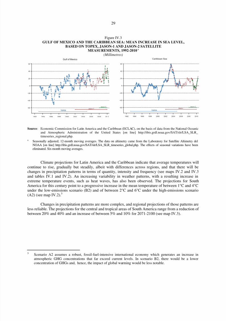
Comparisons of historical records on sea levels indicate that they have been rising in the Gulf of Mexico and the Caribbean Sea (see figure IV.3). The increase is greater for the Gulf of Mexico, witha trend of about 2.8 mm ± 0.3 mm per year, while the increase for the Caribbean Sea is 1.6 mm ± 0.4mm per year.
26.2
26.0
25.8
25.6
25.425.2
25.0
24.8
24.6
24.4
24.2
24.0
23.8
23.6
23.4
23.2
23.0
1960 1964 1968 1972 1976 1980 1984 1988 1992 1996 2000 2004
1988 1992 1996 2000 2004
26.2
26.0
25.8
25.6
25.4
25.2
25.0
24.8
24.6
24.4
24.2
24.0
23.8
23.6
Observed
Linear trend
Quadratic trend
Cubic trend
Polynomial trend (Kernel)
Beveridge-Nelsondecomposition
Smooth transition
Moving average
Holt-Winters filter
Hodrick-Prescott filter
Kalman filter
8/8/2019 CEPAL Climate Change 2010
http://slidepdf.com/reader/full/cepal-climate-change-2010 29/107
29
Figure IV.3GULF OF MEXICO AND THE CARIBBEAN SEA: MEAN INCREASE IN SEA LEVEL,
BASED ON TOPEX, JASON-1 AND JASON-2 SATELLITEMEASUREMENTS, 1992-2010
a
(Millimetres)
Source: Economic Commission for Latin America and the Caribbean (ECLAC), on the basis of data from the National Oceanicand Atmospheric Administration of the United States [on line] http://ibis.grdl.noaa.gov/SAT/slr/LSA_SLR_timeseries_regional.php.
a Seasonally adjusted; 12-month moving averages. The data on altimetry came from the Laboratory for Satellite Altimetry delNOAA [on line] http://ibis.grdl.noaa.gov/SAT/slr/LSA_SLR_timeseries_global.php. The effects of seasonal variations have beeneliminated. Six-month moving averages.
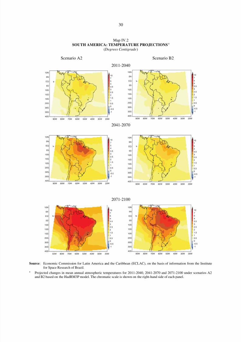
Climate projections for Latin America and the Caribbean indicate that average temperatures will
continue to rise, gradually but steadily, albeit with differences across regions, and that there will bechanges in precipitation patterns in terms of quantity, intensity and frequency (see maps IV.2 and IV.3and tables IV.1 and IV.2). An increasing variability in weather patterns, with a resulting increase inextreme temperature events, such as heat waves, has also been observed. The projections for SouthAmerica for this century point to a progressive increase in the mean temperature of between 1°C and 4°Cunder the low-emissions scenario (B2) and of between 2°C and 6°C under the high-emissions scenario(A2) (see map IV.2).5
Changes in precipitation patterns are more complex, and regional projections of those patterns areless reliable. The projections for the central and tropical areas of South America range from a reduction of between 20% and 40% and an increase of between 5% and 10% for 2071-2100 (see map IV.3).
5 Scenario A2 assumes a robust, fossil-fuel-intensive international economy which generates an increase inatmospheric GHG concentrations that far exceed current levels. In scenario B2, there would be a lowerconcentration of GHGs and, hence, the impact of global warming would be less notable.
−60
−40
−20
0
20
40
60
************************************************
**********************************************************************************
*********************************************
********************************************
************************
*************************************
***********
1992 1994 1996 1998 2000 2002 2004 2006 2008 2010
TOPEX
Jason-1Jason-2
Caribbean Sea
−60
−40
−20
0
20
40
60
***********
********************************************************
**************************
*****
**
*****
***************
*******************************************************
*******************************************
**************
************
*****************************************
*
*****
1992 1994 1996 1998 2000 2002 2004 2006 2008 2010
TOPEX
Jason-1Jason-2
Gulf of Mexico
8/8/2019 CEPAL Climate Change 2010
http://slidepdf.com/reader/full/cepal-climate-change-2010 30/107
30
Map IV.2SOUTH AMERICA: TEMPERATURE PROJECTIONS
a
( Degrees Centigrade)
Scenario A2 Scenario B22011-2040
2041-2070
2071-2100
Source: Economic Commission for Latin America and the Caribbean (ECLAC), on the basis of information from the Institutefor Space Research of Brazil.
a Projected changes in mean annual atmospheric temperatures for 2011-2040, 2041-2070 and 2071-2100 under scenarios A2and B2 based on the HadRM3P model. The chromatic scale is shown on the right-hand side of each panel.
10N
5N
EQ
5S
10S
15S
10S
25S
30S
35S
40S
10
7
5
4
3.5
3
2.5
2
1.5
1
0.5
0
-0.5
-1
90W 80W 70W 60W 50W 40W 30W 20W
10N
5N
EQ
5S
10S
15S
10S
25S
30S
35S
40S
10
7
5
4
3.5
3
2.5
2
1.5
1
0.5
0
-0.5
-1
90W 80W 70W 60W 50W 40W 30W 20W
10N
5N
EQ
5S
10S
15S
10S
25S
30S
35S
40S
10
7
5
4
3.5
3
2.5
2
1.5
1
0.5
0
-0.5
-1
90W 80W 70W 60W 50W 40W 30W 20W
10N
5N
EQ
5S
10S
15S
10S
25S
30S
35S
40S
10
7
5
4
3.5
3
2.5
2
1.5
1
0.5
0
-0.5
-1
90W 80W 70W 60W 50W 40W 30W 20W
10N
5N
EQ
5S
10S
15S
10S
25S
30S
35S
40S
10
7
5
4
3.5
3
2.5
2
1.5
1
0.5
0
-0.5
-1
90W 80W 70W 60W 50W 40W 30W 20W
10N
5N
EQ
5S
10S
15S
10S
25S
30S
35S
40S
10
7
5
4
3.5
3
2.5
2
1.5
1
0.5
0
-0.5
-1
90W 80W 70W 60W 50W 40W 30W 20W

8/8/2019 CEPAL Climate Change 2010
http://slidepdf.com/reader/full/cepal-climate-change-2010 31/107
31
Map IV.3SOUTH AMERICA: PRECIPITATION PROJECTIONS
a
(Percentages)
Scenario A2 Scenario B2
2011-2040
2041-2070
2071-2100
Source: Economic Commission for Latin America and the Caribbean (ECLAC), on the basis of information from the Institutefor Space Research of Brazil.
a Projected changes in precipitation for 2011-2040, 2041-2070, 2071-2100 under scenarios A2 and B2, based on the HadRM3Pmodel. The chromatic scale is indicated on the right-hand side of each panel.
90W40S
35S
30S
25S
20S
15S
10S
5S
EQ
5S
10S
-50
-30
-20
-15
-10
-5
0
5
10
15
20
30
50
80W 70W 60W 50W 40W 30W 20W 90W40S
35S
30S
25S
20S
15S
10S
5S
EQ
5S
10S
-50
-30
-20
-15
-10
-5
0
5
10
15
20
30
50
80W 70W 60W 5 0W 40W 30W 20W
90W40S
35S
30S
25S
20S
15S
10S
5S
EQ
5S
10S
-50
-30-20
-15
-10
-5
0
5
10
15
20
30
50
80W 70W 60W 50W 40W 30W 20W 90W40S
35S
30S
25S
20S
15S
10S
5S
EQ
5S
10S
-50
-30-20
-15
-10
-5
0
5
10
15
20
30
50
80W 70W 60W 5 0W 40W 30W 20W
90W40S
35S
30S
25S
20S
15S
10S
5S
EQ
5S
10S
-50
-30
-20
-15-10
-5
0
5
10
15
20
30
50
80W 70W 60W 50W 40W 30W 20W 90W40S
35S
30S
25S
20S
15S
10S
5S
EQ
5S
10S
-50
-30
-20
-15-10
-5
0
5
10
15
20
30
50
80W 70W 60W 5 0W 40W 30W 20W

8/8/2019 CEPAL Climate Change 2010
http://slidepdf.com/reader/full/cepal-climate-change-2010 32/107
32
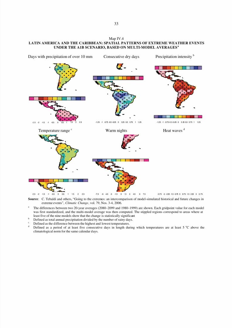
Projections indicate that there will be a steady increase in extreme weather events (see mapIV.4). Rainfall is expected to intensify by 10%, according to the average for the various climatemodels, in central Mexico, the tropics and the south-eastern regions of South America, with an upwardtrend in north-western Ecuador, Peru and south-eastern South America, and declines in Amazonia,
north-eastern Brazil, the northern central portion of Chile and most of Mexico and Central America.Projections of consecutive dry days point towards increases in Mexico, Central America and all of South America except Ecuador, north-eastern Peru and Colombia, with the upward or downwardchanges in precipitation being estimated at less than 10%. Although precipitation intensity is increasingin most of Latin America and Central America, the amount of time between one rainfall and the nexttends to be longer (more consecutive dry days), and average precipitation levels have been declining. Inaddition, temperatures have been higher in most of South and Central America. A significant increasein heat waves is projected for the entire region, and particularly the Caribbean, south-eastern SouthAmerica and Central America. A steady and considerable rise in the number of warm nights is alsoexpected for all of Latin America and especially for Mexico, Central America and the subtropicalportions of South America.
The climate-change patterns projected for Latin America up to the year 2100 are summarized inmap IV.5. The projected changes are based on variations in the projected averages and extremes, asshown in Meehl and others (2007), Christensen and others (2007) and Magrin and others (2007).
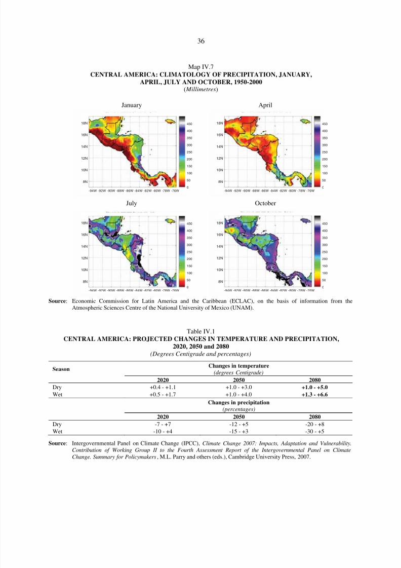
The available evidence for 1950-2000 for Central America points to higher temperatures andgreater variability (see map IV.6). Precipitation maps indicate that rainfall was generally concentrated inthe months from May to October and show the differing patterns of rainfall along the Atlantic and Pacificcoasts and in the northern and southern areas of the isthmus (see map IV.7). In addition, there is a highdegree of year-on-year variability associated with the El Niño-Southern Oscillation (ENSO). Theprojected changes are summed up in table IV.1.
8/8/2019 CEPAL Climate Change 2010
http://slidepdf.com/reader/full/cepal-climate-change-2010 33/107
33
Map IV.4LATIN AMERICA AND THE CARIBBEAN: SPATIAL PATTERNS OF EXTREME WEATHER EVENTS
UNDER THE A1B SCENARIO, BASED ON MULTI-MODEL AVERAGESa
Days with precipitation of over 10 mm Consecutive dry days Precipitation intensityb
Temperature range c Warm nights Heat waves d
Source: C. Tebaldi and others, “Going to the extremes: an intercomparison of model-simulated historical and future changes inextreme events”, Climatic Change, vol. 79, Nos. 3-4, 2006.
a The differences between two 20-year averages (2080–2099 and 1980–1999) are shown. Each gridpoint value for each modelwas first standardized, and the multi-model average was then computed. The stippled regions correspond to areas where atleast five of the nine models show that the change is statistically significant
b Defined as total annual precipitation divided by the number of rainy days.c Defined as the difference between the highest and lowest temperatures.d Defined as a period of at least five consecutive days in length during which temperatures are at least 5oC above the
climatological norm for the same calendar days.
-2-2.5 -1.5 -1 -0.5 0 0.5 1 1.5 2 2.5 -1-1.25 -0.75 -0.5 -0.25 0 0.25 0.5 0.75 1 1.25 -1-1.25 -0.75-0.5 -0.25 0 0.25 0.5 0.75 1 1.25
-3-3.75 -2.25 -1.5 -0.75 0 0.75 1.5 2.25 3 3.75-6-7.5 -4.5 -3 -1.5 0 1.5 3 4.5 6 7.5-2-2.5 -1.5 -1 -0.5 0 0.5 1 1.5 2 2.5

8/8/2019 CEPAL Climate Change 2010
http://slidepdf.com/reader/full/cepal-climate-change-2010 34/107

8/8/2019 CEPAL Climate Change 2010
http://slidepdf.com/reader/full/cepal-climate-change-2010 35/107
35
Map IV.6CENTRAL AMERICA: CLIMATOLOGY OF MEAN TEMPERATURES FOR
JANUARY, APRIL, JULY AND OCTOBER, 1950-2000( Degrees Centigrade)
January April
July October
Source: Economic Commission for Latin America and the Caribbean (ECLAC), on the basis of information from theAtmospheric Sciences Centre of the National University of Mexico (UNAM).
20N
15N
10N
5N
28
26
24
22
20
18
16
14
12
10
-95W -90W -85W -80W -75W
20N
15N
10N
5N
28
26
24
22
20
18
16
14
12
10
-95W -90W -85W -80W -75W
20N
15N
10N
5N
28
26
24
22
20
18
16
14
12
10
-95W -90W -85W -80W -75W
20N
15N
10N
5N
28
26
24
22
20
18
16
14
12
10
-95W -90W -85W -80W -75W
8/8/2019 CEPAL Climate Change 2010
http://slidepdf.com/reader/full/cepal-climate-change-2010 36/107
36
Map IV.7CENTRAL AMERICA: CLIMATOLOGY OF PRECIPITATION, JANUARY,
APRIL, JULY AND OCTOBER, 1950-2000( Millimetres)
January April
July October
Source: Economic Commission for Latin America and the Caribbean (ECLAC), on the basis of information from theAtmospheric Sciences Centre of the National University of Mexico (UNAM).
Table IV.1CENTRAL AMERICA: PROJECTED CHANGES IN TEMPERATURE AND PRECIPITATION,
2020, 2050 and 2080(Degrees Centigrade and percentages)
SeasonChanges in temperature
(degrees Centigrade) 2020 2050 2080
Dry +0.4 - +1.1 +1.0 - +3.0 +1.0 - +5.0
Wet +0.5 - +1.7 +1.0 - +4.0 +1.3 - +6.6
Changes in precipitation(percentages)
2020 2050 2080
Dry -7 - +7 -12 - +5 -20 - +8
Wet -10 - +4 -15 - +3 -30 - +5
Source: Intergovernmental Panel on Climate Change (IPCC), Climate Change 2007: Impacts, Adaptation and Vulnerability.Contribution of Working Group II to the Fourth Assessment Report of the Intergovernmental Panel on ClimateChange. Summary for Policymakers, M.L. Parry and others (eds.), Cambridge University Press, 2007.
0
50
100
150
200
250
300
350
400
450
8N
-94W -92W -90W -88W -86W -84W -82W -80W -78W -76W
10N
12N
14N
16N
18N
0
50
100
150
200
250
300
350
400
450
8N
-94W -92W -90W -88W -86W -84W -82W -80W -78W -76W
10N
12N
14N
16N
18N
0
50
100
150
200
250
300
350
400
450
8N
-94W -92W -90W -88W -86W -84W -82W -80W -78W -76W
10N
12N
14N
16N
18N
0
50
100
150
200
250
300
350
400
450
8N
-94W -92W -90W -88W -86W -84W -82W -80W -78W -76W
10N
12N
14N
16N
18N

8/8/2019 CEPAL Climate Change 2010
http://slidepdf.com/reader/full/cepal-climate-change-2010 37/107
37
The climate scenarios for the Caribbean, which are subject to a high degree of uncertainty (IPCC,2007a), and for the Atlantic are shown in table IV.2. Available evidence points to a possible increase inextreme weather events, particularly hurricanes.
Table IV.2CLIMATE SCENARIOS FOR THE CARIBBEAN AND THE ATLANTIC COAST
Climate variable Climate scenario
TemperatureA projected increase of between 0.8°C and 2.5°C by 2050 and of 0.9°C -4°C by 2080
PrecipitationA variation of from -36.3% to +34.2% is expected by 2050 and of from -49.3% to +28.9% by the end of the century
Sea level May rise by 35 cm by the end of the century
Extreme weather eventsA 5%-10% increase in the frequency of hurricanes over the course of the century
Source: Economic Commission for Latin America and the Caribbean (ECLAC), on the basis of the Intergovernmental Panel on
Climate Change (IPCC), Climate Change 2007: The Physical Science Basis. Contribution of Working Group I to theFourth Assessment Report of the Intergovernmental Panel on Climate Change, Cambridge University Press, 2007; andClimate Change 2007- Impacts, Adaptation and Vulnerability. Contribution of Working Group II to the Fourth
Assessment Report of the IPCC , Cambridge University Press, 2007.
MAIN MESSAGES
• Scientific evidence demonstrates that global warming associated with increased GHG emissionsfrom anthropogenic activities is giving rise to identifiable changes in the climate, such as risingtemperatures, altered precipitation patterns, a shrinking cryosphere, rising sea levels and shiftingpatterns of extreme weather events. The evidence concerning climate change in Latin America
and the Caribbean is in keeping with the information compiled at the international level, butnevertheless shows some significant differences between the region and the rest of the world.
• The projections calculated under a range of scenarios indicate that there is a very high probabilitythat mean temperatures will increase by between 1oC and 6oC (the greater likelihood being thatthey will climb by between 2oC and 4oC), while precipitation will rise by between 5% and 10% insome areas and decline by between 20% and 40% in others. Glaciers located in the Andeancountries are expected to continue to melt. The patterns of extreme weather events in such areasas the Caribbean, Central America and tropical and subtropical areas of South America areexpected to shift, and climatic phenomena such as El Niño may be altered as well.

8/8/2019 CEPAL Climate Change 2010
http://slidepdf.com/reader/full/cepal-climate-change-2010 38/107
38
V. MACROECONOMIC TRENDS
Over the long term, the growth of the economies of Latin America and the Caribbean is shaped by a
complex web of factors and interrelationships. Nevertheless, a set of regular empirical patterns can beidentified that serve as a basis for the construction of future scenarios and their respective baselines orbusiness-as-usual (BAU) counterparts. The fundamental characteristics of the Latin American andCaribbean economies that can be used to establish these baselines are discussed below.
(a) Taken as a group, the economies of the region, as is true of modern economies elsewhere, arewitnessing a long-run upward trend in per capita GDP, with some oscillations around the trend line(ECLAC, 2009b). This regular pattern of per capita GDP can be disaggregated into a trend component,which includes regular long-run changes, and a cyclical component, which corresponds to temporarydeviations from the long-term trend. Long-term changes are generally considered to follow adeterministic or stochastic trend, which points to the presence of non-stationary behaviour.
There are various techniques for disaggregating the unobservable components of the trend,although there is no consensus as to the best way of specifying the model or arriving at estimates or, inmost cases, of breaking down the trend’s composition. In addition, different trend models distinguishdifferent cyclical components, with the attendant risk of generating spurious results. The simultaneousapplication of a broad spectrum of methods for disaggregating the series provides a way of obtainingrobust evidence on these regular patterns, and particularly with respect to the existence of an upwardtrend in per capita GDP.
The earlier analysis of trends in per capita GDP presented by ECLAC (2009b) can besupplemented by an examination of per capita GDP valued in 2005 purchasing power parity (PPP)dollars, since the focus is on providing a clearer picture of the conditions in a given economy as comparedto those in the rest of the world.1 An analysis of unobserved components of per capita GDP in PPP terms
for Latin America and the Caribbean confirms the presence of a long-term trend, but the exact value of that trend remains quite uncertain (see figure V.1 and table V.1).
Per capita GDP growth rates have varied over time. The mean historical per capita GDP growthrate (1980-2009) for Latin America and the Caribbean is fairly low, at 0.83% per year (see figure V.2 andtable V.2), but this is the average of sharply differing annual per capita GDP growth rates of 0.68% for1980-1990 (known as the “lost decade” for Latin America), 1.55% for 1990-2000 and 1.73% for 2000-2009. These figures indicate that the pace of economic growth in the region has been on the rise, asreflected in the gradual shift to the right of the distribution of probabilities for PPP per capita GDP growthrates (see the lower left panel of figure V.2). The trend for Latin America and the Caribbean is lessfavourable than the trend for other regions of the world (see table V.3), and this would appear to indicatethat the region’s economic growth rates will be above the historic mean in the future.
1 This does not, in the aggregate, alter the results presented earlier, although some of the figures differ (e.g.,reported growth rates).
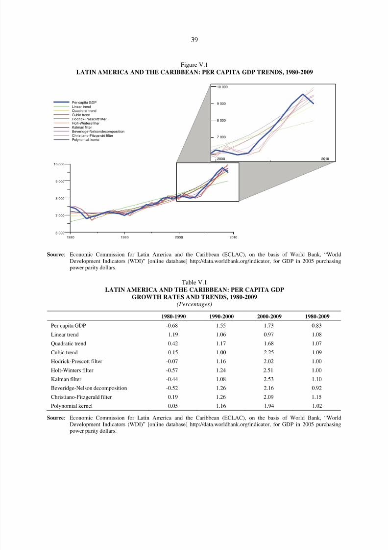
8/8/2019 CEPAL Climate Change 2010
http://slidepdf.com/reader/full/cepal-climate-change-2010 39/107
39
Figure V.1LATIN AMERICA AND THE CARIBBEAN: PER CAPITA GDP TRENDS, 1980-2009
Source: Economic Commission for Latin America and the Caribbean (ECLAC), on the basis of World Bank, “WorldDevelopment Indicators (WDI)” [online database] http://data.worldbank.org/indicator, for GDP in 2005 purchasingpower parity dollars.
Table V.1
LATIN AMERICA AND THE CARIBBEAN: PER CAPITA GDPGROWTH RATES AND TRENDS, 1980-2009
(Percentages)
1980-1990 1990-2000 2000-2009 1980-2009
Per capita GDP -0.68 1.55 1.73 0.83
Linear trend 1.19 1.06 0.97 1.08
Quadratic trend 0.42 1.17 1.68 1.07
Cubic trend 0.15 1.00 2.25 1.09
Hodrick-Prescott filter -0.07 1.16 2.02 1.00
Holt-Winters filter -0.57 1.24 2.51 1.00
Kalman filter -0.44 1.08 2.53 1.10
Beveridge-Nelson decomposition -0.52 1.26 2.16 0.92
Christiano-Fitzgerald filter 0.19 1.26 2.09 1.15
Polynomial kernel 0.05 1.16 1.94 1.02
Source: Economic Commission for Latin America and the Caribbean (ECLAC), on the basis of World Bank, “WorldDevelopment Indicators (WDI)” [online database] http://data.worldbank.org/indicator, for GDP in 2005 purchasingpower parity dollars.
1980 1990 2000 2010
10 000
9 000
8 000
7 000
7 000
6 000
10 000
9 000
8 000
2000 2010
Per capita GDP
Linear trendQuadratic trendCubic trend
Hodrick-Prescott filterHolt-Winters filterKalman filter
Beveridge-Nelson decompositionChristiano-Fitzgerald filterPolynomial kernel
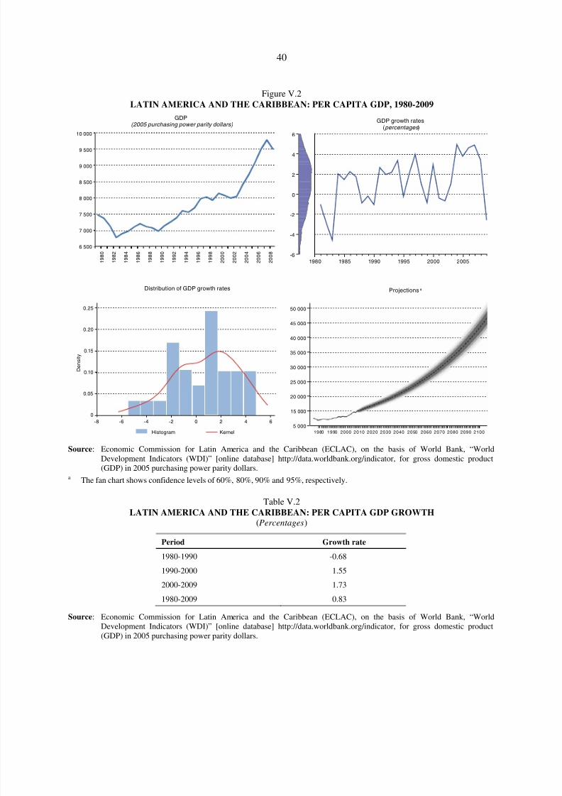
8/8/2019 CEPAL Climate Change 2010
http://slidepdf.com/reader/full/cepal-climate-change-2010 40/107
40
Figure V.2LATIN AMERICA AND THE CARIBBEAN: PER CAPITA GDP, 1980-2009
Source: Economic Commission for Latin America and the Caribbean (ECLAC), on the basis of World Bank, “WorldDevelopment Indicators (WDI)” [online database] http://data.worldbank.org/indicator, for gross domestic product(GDP) in 2005 purchasing power parity dollars.
a The fan chart shows confidence levels of 60%, 80%, 90% and 95%, respectively.
Table V.2LATIN AMERICA AND THE CARIBBEAN: PER CAPITA GDP GROWTH
(Percentages)
Period Growth rate
1980-1990 -0.681990-2000 1.55
2000-2009 1.73
1980-2009 0.83
Source: Economic Commission for Latin America and the Caribbean (ECLAC), on the basis of World Bank, “WorldDevelopment Indicators (WDI)” [online database] http://data.worldbank.org/indicator, for gross domestic product(GDP) in 2005 purchasing power parity dollars.
-6
-4
-2
0
2
4
6
1980 1985 1990 1995 2000 2005
10 000
9 500
9 000
8 500
8 000
7 500
7 000
6 500
1 9 8 0
1 9 8 2
1 9 8 4
1 9 8 6
1 9 8 8
1 9 9 0
1 9 9 2
1 9 9 4
1 9 9 6
1 9 9 8
2 0 0 0
2 0 0 2
2 0 0 4
2 0 0 6
2 0 0 8
0.25
0.20
0.15
0.10
0.05
0
D e n s i t y
-8 -6 -4 -2 0 2 4 6
Histogram Kernel
GDP(2005 purchasing power parity dollars)
GDP growth rates(percentages )
Distribution of GDP growth rates Projections a
1980 1990 2000 2010 2020 2030 2040 2050 2060 2070 2080 2090 2100
50 000
45 000
40 000
35 000
30 000
25 000
20 000
15 000
5 000

8/8/2019 CEPAL Climate Change 2010
http://slidepdf.com/reader/full/cepal-climate-change-2010 41/107
41
Table V.3WORLD REGIONS: PER CAPITA GDP GROWTH
(Percentages)
Region 1980-1990 1990-2000 2000-2009 1980-2009
Euro zone 2.12 1.88 0.55 1.55
Organisation for Economic Co-operation and Development (OECD) 2.45 2.01 0.87 1.80
North America 2.21 2.04 0.66 1.67
Latin America and the Caribbean -0.68 1.55 1.73 0.83
Middle East and West Africa -1.33 1.70 2.32 0.83
Sub-Saharan Africa -1.05 -0.30 2.51 0.30
East Asia and Asia and the Pacific 3.79 3.56 4.71 3.99
South Asia 3.19 3.26 5.30 3.86
World 1.37 1.47 2.11 1.63
Source: Economic Commission for Latin America and the Caribbean (ECLAC), on the basis of World Bank, “World
Development Indicators (WDI)” [online database] http://data.worldbank.org/indicator, for gross domestic product(GDP) in 2005 purchasing power parity dollars.
Per capita GDP trends in the region can also be gauged using an autoregressive integrated movingaverage (ARIMA) model, along with the corresponding probabilities distribution function (fan chart).2 The available information, which includes trend curves, the ARIMA model and the correspondingprobability distribution, and evidence on the recent upswing in the region’s growth and internationaltrends, suggests that, with a 60% probability, Latin America’s per capita GDP growth rate, measured inPPP terms, will range between 1.63% and 1.75% in the coming years, with a BAU mean of 1.69%. Thisprojection can be graphed directly onto the per capita GDP series (lower right panel of figure V.2).
(b) The significant differences that exist across the economies of Latin America and the Caribbeanare in keeping with international evidence. Available data indicate that the per capita GDP curves for thecountries of Latin America and the Caribbean are not on course for absolute convergence (convergence )(ECLAC, 2009b), i.e., the growth rate for countries with lower per capita GDP levels is not higher thanthe rate for countries with higher per capita GDP levels. International evidence also shows that for 1980–2009 there was no absolute convergence at the international level either (see figure V.3),3 and trendsdiffer from one region or group of countries to the next. In fact, the figures for all the regions other thanAfrica yield a negative correlation between per capita GDP growth rates and initial per capita incomelevels (see figure V.3). The trends from one world region to the next are also very uneven.
2 Figures for 2009 were not used in these calculations because of their anomalous nature, which would distort theprojections.
3 The result depends, to a great extent, on the type of per capita GDP figures that are used in the calculation,however.
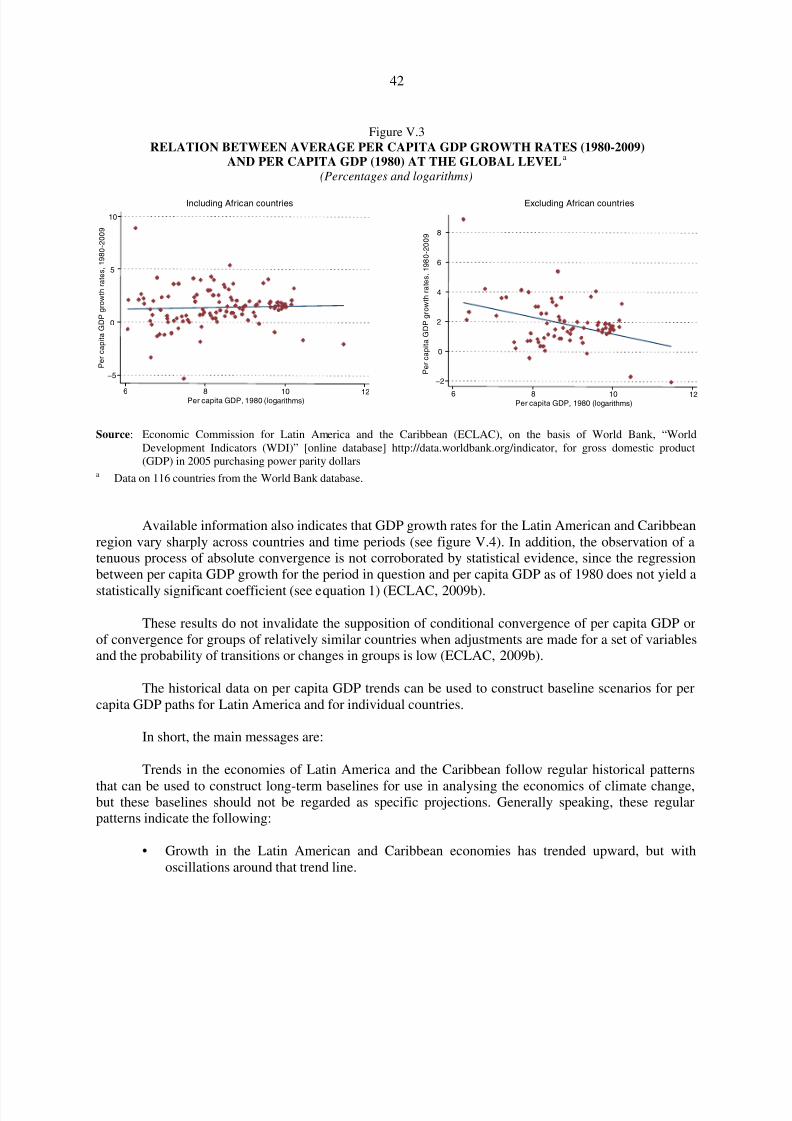
8/8/2019 CEPAL Climate Change 2010
http://slidepdf.com/reader/full/cepal-climate-change-2010 42/107
42
Figure V.3RELATION BETWEEN AVERAGE PER CAPITA GDP GROWTH RATES (1980-2009)
AND PER CAPITA GDP (1980) AT THE GLOBAL LEVELa
(Percentages and logarithms)
Source: Economic Commission for Latin America and the Caribbean (ECLAC), on the basis of World Bank, “WorldDevelopment Indicators (WDI)” [online database] http://data.worldbank.org/indicator, for gross domestic product(GDP) in 2005 purchasing power parity dollars
a Data on 116 countries from the World Bank database.
Available information also indicates that GDP growth rates for the Latin American and Caribbeanregion vary sharply across countries and time periods (see figure V.4). In addition, the observation of atenuous process of absolute convergence is not corroborated by statistical evidence, since the regressionbetween per capita GDP growth for the period in question and per capita GDP as of 1980 does not yield a
statistically significant coefficient (see equation 1) (ECLAC, 2009b).
These results do not invalidate the supposition of conditional convergence of per capita GDP orof convergence for groups of relatively similar countries when adjustments are made for a set of variablesand the probability of transitions or changes in groups is low (ECLAC, 2009b).
The historical data on per capita GDP trends can be used to construct baseline scenarios for percapita GDP paths for Latin America and for individual countries.
In short, the main messages are:
Trends in the economies of Latin America and the Caribbean follow regular historical patterns
that can be used to construct long-term baselines for use in analysing the economics of climate change,but these baselines should not be regarded as specific projections. Generally speaking, these regularpatterns indicate the following:
• Growth in the Latin American and Caribbean economies has trended upward, but withoscillations around that trend line.
−2
0
2
4
6
8
6 8 10 12Per capita GDP, 1980 (logarithms)
−5
0
5
10
P e r c
a p
i t a G D P
g r o
w t h
r a t e
s ,
1 9 8
0 - 2
0 0 9
Pe
r c a p
i t a G D P
g r o w
t h r a
t e s
, 1
9 8 0
- 2 0 0 9
6 8 10 12Per capita GDP, 1980 (logarithms)
Including African countries Excluding African countries
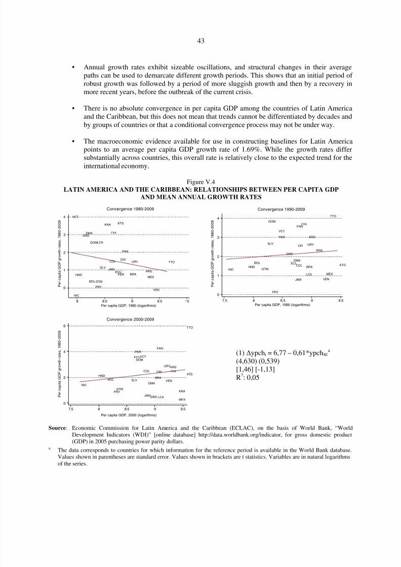
8/8/2019 CEPAL Climate Change 2010
http://slidepdf.com/reader/full/cepal-climate-change-2010 43/107
43
• Annual growth rates exhibit sizeable oscillations, and structural changes in their averagepaths can be used to demarcate different growth periods. This shows that an initial period of robust growth was followed by a period of more sluggish growth and then by a recovery inmore recent years, before the outbreak of the current crisis.
• There is no absolute convergence in per capita GDP among the countries of Latin Americaand the Caribbean, but this does not mean that trends cannot be differentiated by decades andby groups of countries or that a conditional convergence process may not be under way.
• The macroeconomic evidence available for use in constructing baselines for Latin Americapoints to an average per capita GDP growth rate of 1.69%. While the growth rates differsubstantially across countries, this overall rate is relatively close to the expected trend for theinternational economy.
Figure V.4LATIN AMERICA AND THE CARIBBEAN: RELATIONSHIPS BETWEEN PER CAPITA GDP
AND MEAN ANNUAL GROWTH RATES
(1) ypchi = 6,77 – 0,61*ypch80a
(4,630) (0,539)[1,46] [-1,13]R2: 0,05
Source: Economic Commission for Latin America and the Caribbean (ECLAC), on the basis of World Bank, “WorldDevelopment Indicators (WDI)” [online database] http://data.worldbank.org/indicator, for gross domestic product(GDP) in 2005 purchasing power parity dollars.
a The data corresponds to countries for which information for the reference period is available in the World Bank database.Values shown in parentheses are standard error. Values shown in brackets are t statistics. Variables are in natural logarithmsof the series.
ATG
ARG
BOL
BRA
CHL
COLCRI
DMA
DOM
ECU
SLV
GRD
GTM
HND
JAM
MEX
NIC
PAN
PRY
PER
KNA
LCA
VCT
TTOURY
VEN0
1
2
3
4
P e r c a p i t a G D P g r o w t h r a t e s , 1 9 8 0 - 2 0 0 9
P e r c a p i t a G D P g r o w t h r a t e s , 1 9 8 0 - 2 0 0 9
P e r c a p i t a G D P g r o w t h r a t e s , 1 9 8 0 - 2 0 0 9
8 8.5 9 9.5 10
Per capita GDP, 1980 (logarithms)
ATG
ARG
BOL
BRA
CHL
COL
CRI
DMA
DOM
ECU
SLV
GRD
GTMHND
JAM
MEX
NIC
PAN
PRY
PER
KNA
LCA
VCT
TTO
URY
VEN
0
1
2
3
4
7.5 8 8.5 9 9.5
Per capita GDP, 1990 (logarithms)
ATG
ARG
BOLBRA
CHLCOL CRI
DMA
DOMECU
SLV
GRD
GTM
HND
JAM
MEX
NIC
PAN
PRY
PER
KNA
LCA
VCT
TTO
URY
VEN
0
2
4
6
7.5 8 8.5 9 9.5
Per capita GDP, 2000 (logarithms)
Convergence 1980-2009 Convergence 1990-2009
Convergence 2000-2009
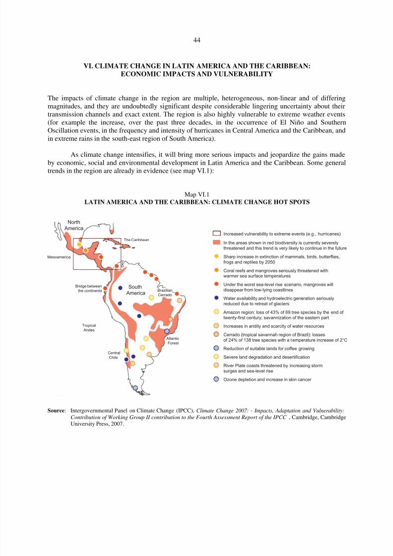
8/8/2019 CEPAL Climate Change 2010
http://slidepdf.com/reader/full/cepal-climate-change-2010 44/107
44
VI. CLIMATE CHANGE IN LATIN AMERICA AND THE CARIBBEAN:ECONOMIC IMPACTS AND VULNERABILITY
The impacts of climate change in the region are multiple, heterogeneous, non-linear and of differingmagnitudes, and they are undoubtedly significant despite considerable lingering uncertainty about theirtransmission channels and exact extent. The region is also highly vulnerable to extreme weather events(for example the increase, over the past three decades, in the occurrence of El Niño and SouthernOscillation events, in the frequency and intensity of hurricanes in Central America and the Caribbean, andin extreme rains in the south-east region of South America).
As climate change intensifies, it will bring more serious impacts and jeopardize the gains madeby economic, social and environmental development in Latin America and the Caribbean. Some generaltrends in the region are already in evidence (see map VI.1):
Map VI.1LATIN AMERICA AND THE CARIBBEAN: CLIMATE CHANGE HOT SPOTS
Source: Intergovernmental Panel on Climate Change (IPCC), Climate Change 2007: - Impacts, Adaptation and Vulnerability:Contribution of Working Group II contribution to the Fourth Assessment Report of the IPCC , Cambridge, CambridgeUniversity Press, 2007.
Central
Chile
Tropical
Andes
Bridge between
the continents
Mesoamerica
The Caribbean
Sharp increase in extinction of mammals, birds, butterflies,
frogs and reptiles by 2050
Coral reefs and mangroves seriously threatened withwarmer sea surface temperatures
Under the worst sea-level rise scenario, mangroves will
disappear from low-lying coastlinesWater availability and hydroelectric generation seriously
reduced due to retreat of glaciers
Amazon region: loss of 43% of 69 tree species by the end of
twenty-first century; savannization of the eastern part
Increases in aridity and scarcity of water resources
Cerrado (tropical savannah region of Brazil): losses
of 24% of 138 tree species with a temperature increase of 2°C
Reduction of suitable lands for coffee growing
Severe land degradation and desertification
River Plate coasts threatened by increasing storm
surges and sea-level rise
In the areas shown in red biodiversity is currently severely
threatened and this trend is very likely to continue in the future
Increased vulnerability to extreme events (e.g., hurricanes)
Ozone depletion and increase in skin cancer
South
America
North
America
Atlantic
Forest
BrazilianCerrado
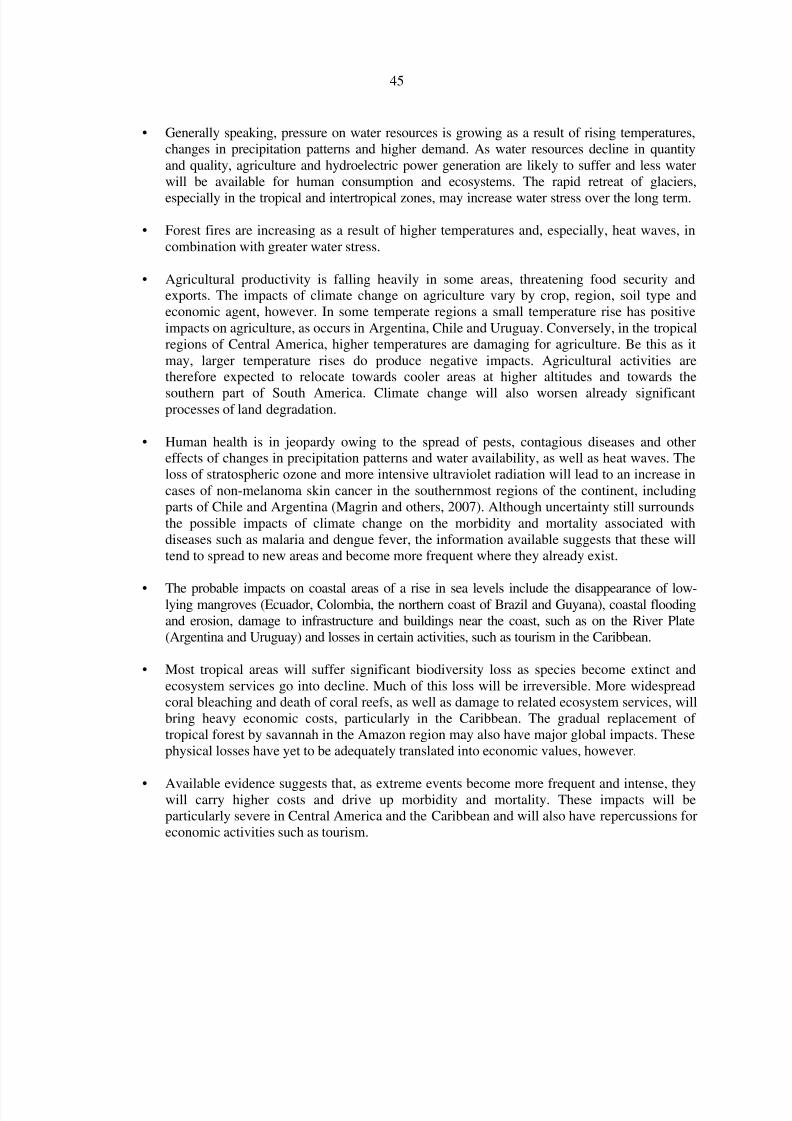
8/8/2019 CEPAL Climate Change 2010
http://slidepdf.com/reader/full/cepal-climate-change-2010 45/107
45
• Generally speaking, pressure on water resources is growing as a result of rising temperatures,changes in precipitation patterns and higher demand. As water resources decline in quantityand quality, agriculture and hydroelectric power generation are likely to suffer and less waterwill be available for human consumption and ecosystems. The rapid retreat of glaciers,
especially in the tropical and intertropical zones, may increase water stress over the long term.
• Forest fires are increasing as a result of higher temperatures and, especially, heat waves, incombination with greater water stress.
• Agricultural productivity is falling heavily in some areas, threatening food security andexports. The impacts of climate change on agriculture vary by crop, region, soil type andeconomic agent, however. In some temperate regions a small temperature rise has positiveimpacts on agriculture, as occurs in Argentina, Chile and Uruguay. Conversely, in the tropicalregions of Central America, higher temperatures are damaging for agriculture. Be this as itmay, larger temperature rises do produce negative impacts. Agricultural activities aretherefore expected to relocate towards cooler areas at higher altitudes and towards the
southern part of South America. Climate change will also worsen already significantprocesses of land degradation.
• Human health is in jeopardy owing to the spread of pests, contagious diseases and othereffects of changes in precipitation patterns and water availability, as well as heat waves. Theloss of stratospheric ozone and more intensive ultraviolet radiation will lead to an increase incases of non-melanoma skin cancer in the southernmost regions of the continent, includingparts of Chile and Argentina (Magrin and others, 2007). Although uncertainty still surroundsthe possible impacts of climate change on the morbidity and mortality associated withdiseases such as malaria and dengue fever, the information available suggests that these willtend to spread to new areas and become more frequent where they already exist.
• The probable impacts on coastal areas of a rise in sea levels include the disappearance of low-lying mangroves (Ecuador, Colombia, the northern coast of Brazil and Guyana), coastal floodingand erosion, damage to infrastructure and buildings near the coast, such as on the River Plate(Argentina and Uruguay) and losses in certain activities, such as tourism in the Caribbean.
• Most tropical areas will suffer significant biodiversity loss as species become extinct andecosystem services go into decline. Much of this loss will be irreversible. More widespreadcoral bleaching and death of coral reefs, as well as damage to related ecosystem services, willbring heavy economic costs, particularly in the Caribbean. The gradual replacement of tropical forest by savannah in the Amazon region may also have major global impacts. Thesephysical losses have yet to be adequately translated into economic values, however.
• Available evidence suggests that, as extreme events become more frequent and intense, theywill carry higher costs and drive up morbidity and mortality. These impacts will beparticularly severe in Central America and the Caribbean and will also have repercussions foreconomic activities such as tourism.

8/8/2019 CEPAL Climate Change 2010
http://slidepdf.com/reader/full/cepal-climate-change-2010 46/107
46
At the same time, changes occurring in non-climate factors make the region more vulnerable toclimate change. These include:
(i) Rising rates of deforestation;
(ii) More rapid soil degradation and desertification;(iii) Growing demographic pressure, particularly in urban areas; and(iv) Overexploitation and contamination of natural resources (water, soil and air).
Empirical evidence for Latin America and the Caribbean shows that climate change impacts onthe economies of the region are significant at the aggregate level, and will increase as time goes on. Theimpacts are also highly uneven, however, varying by climate, region, economic sector and agent, and overtime. Their patterns are nonlinear and have specific thresholds. In some cases, such as where biodiversityor human life is concerned, the consequences are irreversible.
The time horizon over which impacts are assessed can also heavily determine the outcome.Climate change may produce temporary gains for some sectors, activities, regions or geographic areas,
but heavy losses for others. In the short term, some regions of Latin America and the Caribbean maybenefit from a temperature rise of less than 2ºC. A small temperature rise in temperate zones, forexample, may push back the agricultural frontier and increase agricultural productivity. Conversely,regions with lower per capita income and poorer adaptation and prevention capacities may sustainconsiderable economic losses as a result of extreme weather events, even in the short term. This mayimpede the adoption of preventive strategies and facilitate the breaching of certain thresholds in thoseregions, thus triggering irreversible impacts on ecosystems and socioeconomic activities.
Be all this as it may, preliminary estimates of the overall economic costs and benefits forLatin America and the Caribbean based on the information available show a negative balance thatgrows over time.
On the basis of information available from the Regional Economics of Climate Change Studies(RECCS) in Latin America and the Caribbean, this chapter offers a selection of economic impacts of climate change estimated on a preliminary basis for three countries: Chile (ECLAC, 2009a), Ecuador1 andUruguay (ECLAC 2010a), and a subregion, Central America (ECLAC, 2010b). The implications for theagricultural sector are discussed for selected countries.
The climate variations associated with A2 and B2 scenarios are superposed on the baselinescenario for the economy of a region, country or sector. The resulting difference therefore represents theeconomic impact of climate change, as discussed in chapter II. The findings presented in the case studieswere obtained from analysis of climate and economic scenarios and should not be treated as preciseprojections of the respective country’s situation over the next 100 years. Estimates of climate changeimpacts on economic activities depend basically on the climate scenarios assumed, the sectors examined,
the economic valuation methodology and time horizon used and the discount rate applied. Accordingly,the valuation of these costs is still strongly debated.
1 The findings come from studies that form part of ongoing research into the economics of climate change inEcuador. The information and figures given here are preliminary and have yet to be validated by the Governmentof Ecuador, which is currently reviewing them.

8/8/2019 CEPAL Climate Change 2010
http://slidepdf.com/reader/full/cepal-climate-change-2010 47/107
47
Box VI.1RISK AND VULNERABILITY TO THE EFFECTS OF CLIMATE CHANGE ON COASTS
OF LATIN AMERICA AND THE CARIBBEAN
The Intergovernmental Panel on Climate Change (IPCC) (2001 and 2007b) has analysed the rise in average sealevels worldwide as one of the possible impacts of global warming. This exercise has provided projections of sea-level rises on the basis of different greenhouse gas (GHG) emission scenarios. Given the broad range of scenarios,recent research has sought responses using a variety of semi-empirical methods, and has observed that average sealevels could rise by approximately 1 metre by the end of the twenty-first century. Not only rising sea levels threatenthe world’s coasts, however. Variation in other coastal agents, such as swell and seawater surface temperature, mayalso embody significant risk and cause damage such as coastal erosion or coral bleaching. Coastal erosion is a globalproblem, since at least 70% of the world’s fine sediment beaches are receding.
IPCC reports have conducted global analyses of such variables as salinity and surface water temperature,but not yet of swell or meteorological tides. There is a great shortage of data on the southern hemisphere in general,and on Latin America and the Caribbean, in particular. A great effort has been made to address the informationshortage in the region by analysing existing data and generating new, high spatial and temporal resolution databaseson swell and tides. This effort pursues two specific aims: to assess the repercussions of climate change on the coastsof the Latin American and Caribbean region and to help forge a better understanding of some the major marine
dynamics at work around the continent.Recent research has also looked at the influence of various climate variables on the coasts of Latin America
and the Caribbean. El Niño and la Niña, for example, have major impacts on the region’s coastal activities, as doesthe Atlantic multidecadal oscillation (AMO), particularly in Argentina and the southern part of Brazil.
Data on the long-term trends of these phenomena and on climate in Latin America and the Caribbean feedinto an assessment of impacts on the region’s coasts. This, in turn, may be integrated with ecological andsocioeconomic vulnerability data to assess risk patterns in different countries. The risks arising from the early stagesof climate change concern beaches, port infrastructure, and coastal ecosystems and populations and are expressed asa difference over the 2010 risk assessment.
BeachesThe erosion of beaches as a result of climate change will impact two of their key functions: tourism and
coastal protection. Use of beaches for tourism purposes is at high risk, basically because of the loss of usable surfacearea, in the eastern and southern Caribbean and along the east coast of Brazil, especially the easternmost tip. Certain
areas of Argentina, Chile, Peru, Ecuador and Mexico are also considered to be at high risk in this regard.Coastal defence is at significant risk owing the landward retreat of beaches in Brazil, northern Argentina,
and virtually all of the Caribbean. On the Pacific coast, high risks are estimated for Ecuador, Peru and certain partsof Chile, Mexico and Central America.
Port infrastructurePort structure operability will be threatened by climate-driven changes in navigability and access, and by
the breaching of port defence structures owing to variations in swell and sea levels. The ports facing the greatest risk of economic losses due to access problems are, initially: Buenos Aires, San Antonio (Chile), Río Grande (Brazil)and Manzanillo (Mexico). The impact of breaching is measured in terms of port operating hours lost. The resultsshow a sharp increase in breaching owing to larger swell in the mid-twenty-first century (if maritime defencestructures remain unchanged) in southern Brazil, the north-eastern region of Mexico and southern Chile. The areasworst affected by breaching caused by higher average sea levels are northern Brazil and the entire Caribbean coast,with increases of up to 25%. The degree of security currently offered by maritime defence structures in the regionwill be heavily reduced throughout the Latin American and Caribbean region.
Flooding of ecosystems and populated areasAnother of the risks assessed is permanent flooding caused by higher sea levels. The main conclusion is
that the entire coast of Latin America and the Caribbean may be affected to a greater or lesser extent, with theresulting impacts on populations and ecosystems.
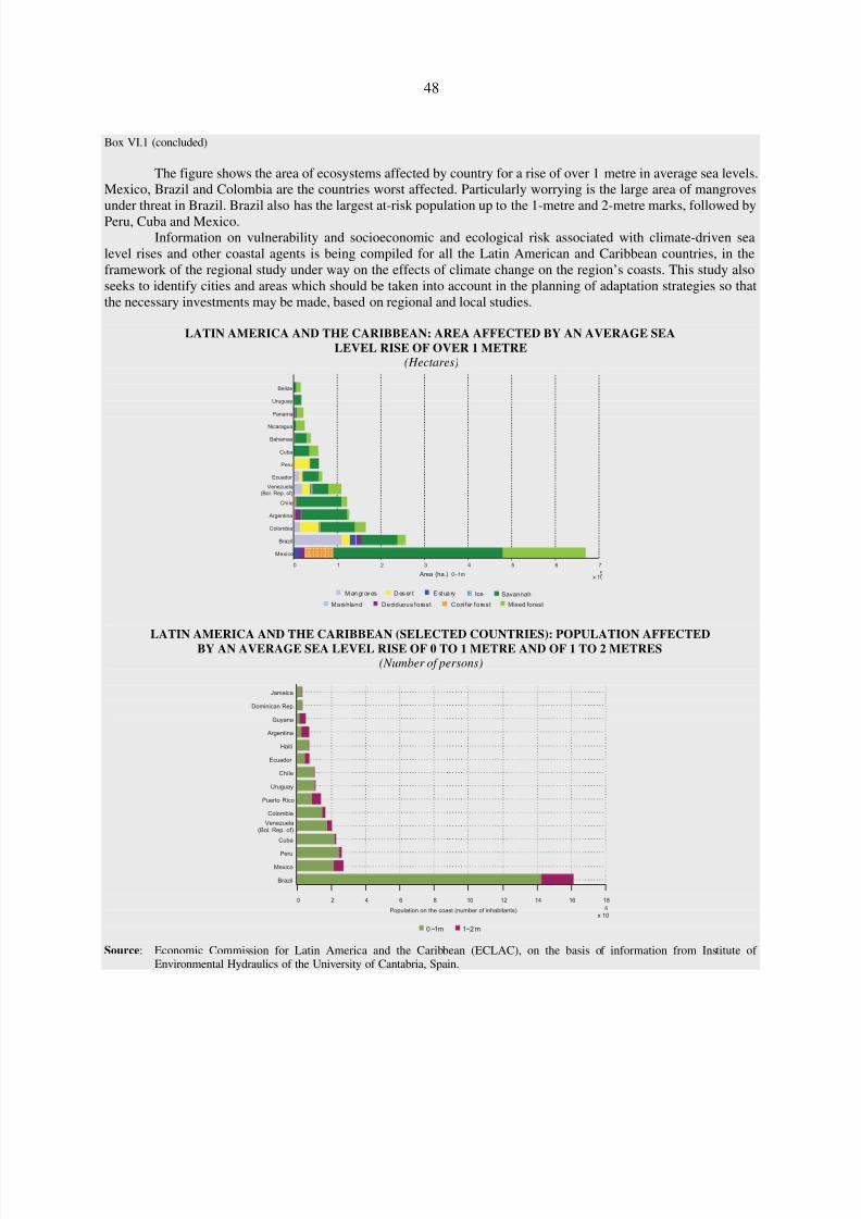
8/8/2019 CEPAL Climate Change 2010
http://slidepdf.com/reader/full/cepal-climate-change-2010 48/107
48
Box VI.1 (concluded)
The figure shows the area of ecosystems affected by country for a rise of over 1 metre in average sea levels.Mexico, Brazil and Colombia are the countries worst affected. Particularly worrying is the large area of mangrovesunder threat in Brazil. Brazil also has the largest at-risk population up to the 1-metre and 2-metre marks, followed byPeru, Cuba and Mexico.
Information on vulnerability and socioeconomic and ecological risk associated with climate-driven sealevel rises and other coastal agents is being compiled for all the Latin American and Caribbean countries, in theframework of the regional study under way on the effects of climate change on the region’s coasts. This study alsoseeks to identify cities and areas which should be taken into account in the planning of adaptation strategies so thatthe necessary investments may be made, based on regional and local studies.
LATIN AMERICA AND THE CARIBBEAN: AREA AFFECTED BY AN AVERAGE SEA
LEVEL RISE OF OVER 1 METRE(Hectares)
LATIN AMERICA AND THE CARIBBEAN (SELECTED COUNTRIES): POPULATION AFFECTED
BY AN AVERAGE SEA LEVEL RISE OF 0 TO 1 METRE AND OF 1 TO 2 METRES(Number of persons)
Source: Economic Commission for Latin America and the Caribbean (ECLAC), on the basis of information from Institute of Environmental Hydraulics of the University of Cantabria, Spain.
Area (ha.) 0−1m
0 1 2 3 4 5 6 7
x 105
Mexico
Brazil
Colombia
Argentina
Chile
Venezuela
(Bol. Rep. of)
Ecuador
Peru
Cuba
Bahamas
Nicaragua
Panama
Uruguay
Belize
Man gr ov es D es er t E st ua ry
Marshland Deciduous forest Conifer forest
Ice Savannah
Mixed forest
Population on the coast (number of inhabitants)
0 2 4 6 8 10 12 14 16 18
x 105
Brazil
Mexico
Peru
Cuba
Venezuela(Bol. Rep. of)
Colombia
Puerto Rico
Uruguay
Chile
Ecuador
Haiti
Argentina
Guyana
Dominican Rep.
Jamaica
0 −1m 1−2 m

8/8/2019 CEPAL Climate Change 2010
http://slidepdf.com/reader/full/cepal-climate-change-2010 49/107
49
A. IMPACTS OF CLIMATE CHANGE IN CHILE
Chile has many features that make it vulnerable to the effects of climate change. Much of its territory has
low precipitation levels associated with desert and semi-arid climates. Many of its water basins and theirinhabitants depend on hydrological systems that revolve around the melting of winter snows. Thecountry’s main economic activities depend directly or indirectly on weather conditions and although thelong coast provides resources, the costal infrastructure also suffers climate impacts and inclemency.Lastly, several areas boast many endemic species and are among the planet’s biodiversity hot spots.
The results provided in this report show broad evidence of the potential impacts of climatechange in Chile. Figures VI.2 and VI.3 show the expected changes in temperature and precipitation inthe A2 climate scenario for the three periods examined in the study: early (2010-2039), intermediate(2040-2069) and late (2070-2099). According to global climate modelling, for Chile climate changemeans, broadly speaking, rising temperatures throughout the country, intensifying as the twenty-firstcentury progresses (around 4°C by the end of the century) and movement away from the sea. These
models also project significant reductions in precipitation (around 30% by the end of the century) in thecentral zone of Chile (between Valparaíso and the region of Los Lagos). In the far north of the country(the regions of Arica to Atacama) the situation is uncertain. In the far south (Magallanes region), themodels indicate a gradual increase in precipitation. Lastly, the Aysen region is a transition zone, whereno major variations are expected with respect to the current situation.
These changes in weather conditions may bring a series of economic, social and environmentalproblems. Many of these will be associated with changes in water resource availability and the resultingeffects on hydroelectric power generation, drinking water supply and the use of water for irrigation andother production sector activities, including manufacturing and mining.
With regard to electric power generation, the scenarios assessed suggest losses of between 10%
and 20% with respect to the baseline situation, with an associated economic cost in the range of US$ 100 million per year. In addition, the increase in thermal power generation needed to compensate forthe loss of hydroelectric sources would increase GHG emissions by around 3 million tons of C02 eq.
With regard to drinking-water supply, the study findings indicate hydrological changes in theRiver Maipo, the main source of water for the metropolitan region, leading to a water supply deficit withrespect to the projected demand of the population. This situation is shared by other Latin American citiesthat depend on Andean snowmelt for their water supply. One of the consequences of this is that waterutilities may have to purchase rights to ensure water supply, and these costs are likely to be passed on tousers in the form of higher rates. This, moreover, would be only one component of the expected impactsof a supply shortage: the changes that would have to be made in the infrastructure to ensure adequateservice would carry other costs, as well.
Evaluation of the impacts on the mining sector suggests that, over the next 30 years, climateconditions —higher temperatures (and thus evaporation) and declining precipitation— will reduce wateravailability in all the basins where mines currently operate. The great majority of mining operations arealready hard pressed for water. The last resort for mines would be seawater desalination, which wouldsignificantly push up production costs —by between US¢ 6 and US¢ 20 per pound of copper— andincrease GHG emissions because of the electricity consumed in the desalination process.

8/8/2019 CEPAL Climate Change 2010
http://slidepdf.com/reader/full/cepal-climate-change-2010 50/107
50
Map VI.2
CHILE: PROJECTED TEMPERATURE CHANGES IN CLIMATE
CHANGE SCENARIO A2, 2010-2099(Changes in degrees Centigrade over historical base)
Source: Economic Commission for Latin America and the Caribbean (ECLAC), La economía del cambio climático en Chile.Síntesis (LC/W.288), Santiago, Chile, 2009.
0
55
50
45
40
35
L a t i t u d e
30
25
20
0.5 1 1.5 2 2.5 3 3.5 4 4.5 (°C)
2010-2039 2040-2069 2070-2099
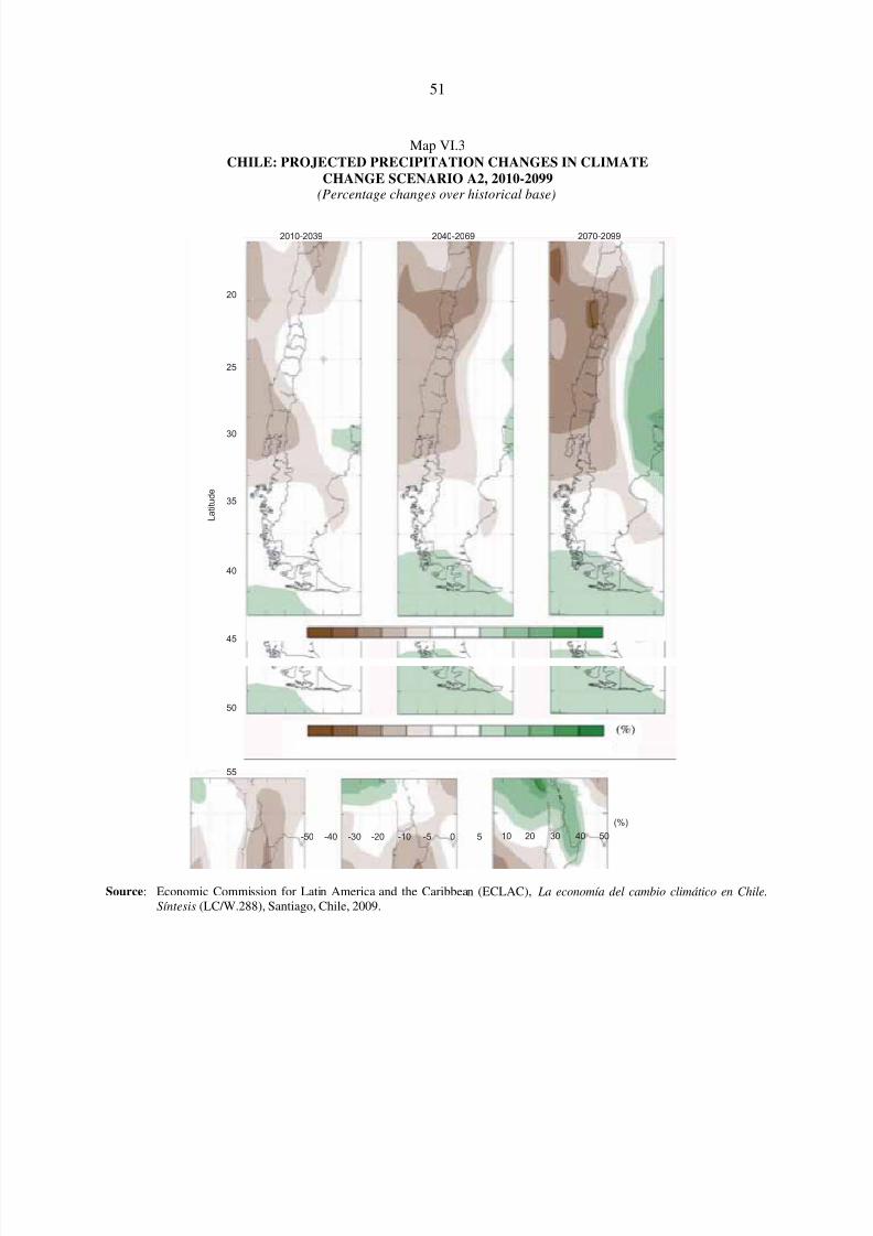
8/8/2019 CEPAL Climate Change 2010
http://slidepdf.com/reader/full/cepal-climate-change-2010 51/107
51
Map VI.3CHILE: PROJECTED PRECIPITATION CHANGES IN CLIMATE
CHANGE SCENARIO A2, 2010-2099(Percentage changes over historical base)
Source: Economic Commission for Latin America and the Caribbean (ECLAC), La economía del cambio climático en Chile.Síntesis (LC/W.288), Santiago, Chile, 2009.
L a t i t u d e
-50 -40 -30 -20 -10 -5 0 5 10 20 30 40 50
(%)
20
2010-2039 2040-2069 2070-2099
25
30
35
40
45
50
55
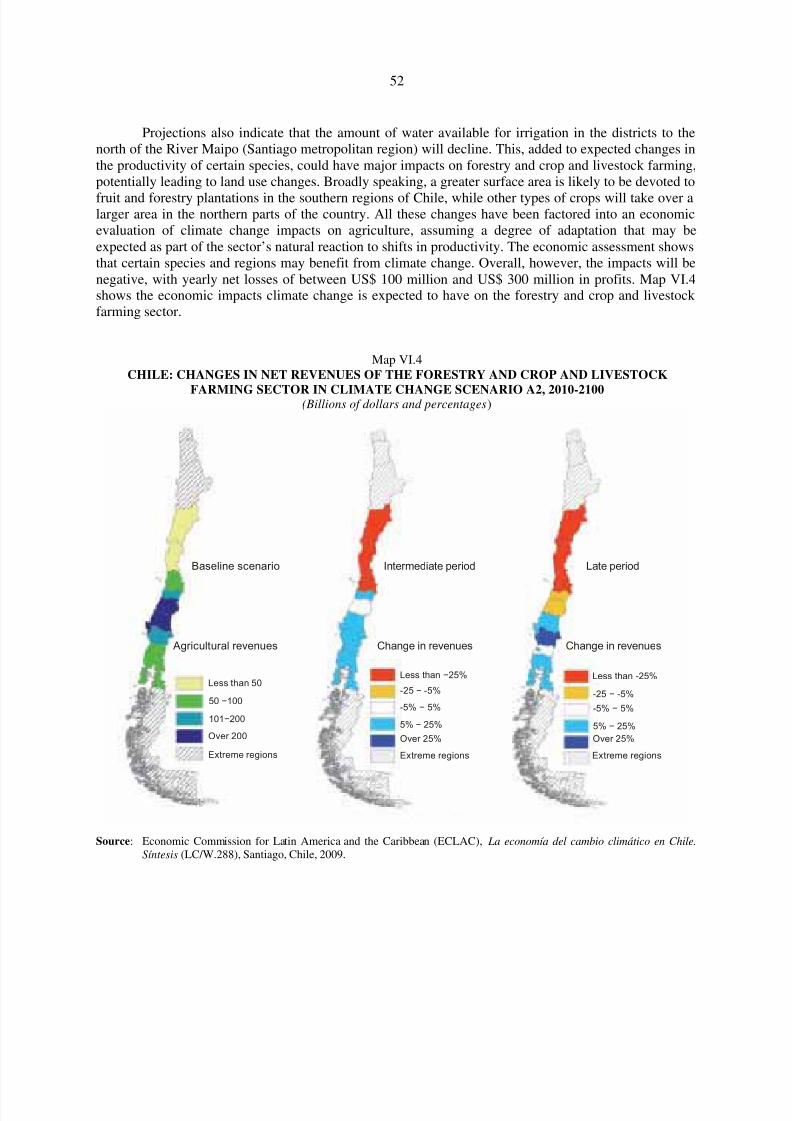
8/8/2019 CEPAL Climate Change 2010
http://slidepdf.com/reader/full/cepal-climate-change-2010 52/107
52
Projections also indicate that the amount of water available for irrigation in the districts to thenorth of the River Maipo (Santiago metropolitan region) will decline. This, added to expected changes inthe productivity of certain species, could have major impacts on forestry and crop and livestock farming,potentially leading to land use changes. Broadly speaking, a greater surface area is likely to be devoted to
fruit and forestry plantations in the southern regions of Chile, while other types of crops will take over alarger area in the northern parts of the country. All these changes have been factored into an economicevaluation of climate change impacts on agriculture, assuming a degree of adaptation that may beexpected as part of the sector’s natural reaction to shifts in productivity. The economic assessment showsthat certain species and regions may benefit from climate change. Overall, however, the impacts will benegative, with yearly net losses of between US$ 100 million and US$ 300 million in profits. Map VI.4shows the economic impacts climate change is expected to have on the forestry and crop and livestock farming sector.
Map VI.4
CHILE: CHANGES IN NET REVENUES OF THE FORESTRY AND CROP AND LIVESTOCK
FARMING SECTOR IN CLIMATE CHANGE SCENARIO A2, 2010-2100(Billions of dollars and percentages)
Source: Economic Commission for Latin America and the Caribbean (ECLAC), La economía del cambio climático en Chile.Síntesis (LC/W.288), Santiago, Chile, 2009.
Baseline scenario Intermediate period Late period
Agricultural revenues Change in revenues Change in revenues
Less than 50Less than −25% Less than -25%
50 −100-25 − -5% -25 − -5%
101−200
-5% − 5% -5% − 5%
Over 200
5% − 25% 5% − 25%
Over 25% Over 25%
Extreme regions Extreme regions Extreme regions

8/8/2019 CEPAL Climate Change 2010
http://slidepdf.com/reader/full/cepal-climate-change-2010 53/107
53
Economic evaluations of climate change impacts were conducted for all the sectors mentioned,except for mining. The impacts were projected in accordance with the economic situation expected in thefuture (based on GDP projections) then aggregated at net present value. In absolute terms, aggregation of the present value of impacts suggests that the costs associated with the A2 scenario vary from
US$ 22 billion to US$ 320 billion at 2008 prices, depending on the discount rate applied and the timehorizon considered. In the B2 scenario, the situation is more ambiguous, since the results range from a netgain of US$ 25 billion to a cost of US$ 40 billion, again depending on the discount rate applied and thetime horizon considered. By way of reference, the country’s GDP for 2008 was about US$ 120 billion.These costs imply that Chile stands to lose the equivalent of 1.1% of GDP annually throughout theanalysis period — up to 2100— in the A2 scenario. Table VI.1 shows the expected direct and indirectcosts of climate change and map VI.5 shows the consolidated impacts for the A2 scenario.
It has not yet been possible to conduct economic impact assessments in a number of other areaswhich may suffer adverse impacts from climate change, including biodiversity and ecosystem services;health; fishing and aquaculture resources; rising sea levels and coastal impacts; extreme events;infrastructure; and changes in energy demand. Assessment in these areas has been hindered by two
factors: (i) in some sectors, such as mining, scientific knowledge has progressed far enough to relateclimate change to physical variables, but the tools are still lacking to translate this into an economicevaluation; and (ii) in other sectors, such as fishing, the basic scientific knowledge still falls short of linking climate change to major biophysical variables. The values given must therefore be viewed asminimum reference values, since they do not include the economic impacts associated with those sectorswhich have not been assessed.
A great challenge lies ahead for Chile with regard to climate change. On the one hand, the country’sdevelopment contributes to causing the problems through growing GHG emissions. On the other, climatechange has economic, social and environmental impacts that threaten development, especially for the mostvulnerable inhabitants. Accordingly, adaptation schemes are needed to soften the adverse impacts. Thechallenge is to break the vicious cycle that is threatening the sustainable development of future generations.
Table VI.1CHILE: AGGREGATE ECONOMIC COSTS IN CLIMATE CHANGE
SCENARIOS A2 AND B2, UP TO 2100 (Millions of dollars)
Sector Discount rate 6% Discount rate 4% Discount rate 2% Discount rate 0,5%
A2 B2 A2 B2 A2 B2 A2 B2
Crop-growing -10 599 -9 734 -26 505 -26 639 -79 165 -86 730 -201 361 -232 875
Fruit-growing 36 104 21 037 77 902 40 248 208 685 96 459 503 568 219 311
Forestry -5 305 -4 610 -12 019 -10 738 -32 308 -29 609 -76 349 -71 068
Livestock 2 036 962 3 147 298 6 807 -2 051 16 119 -6 853Hydroelectric 7 733 6 367 15 026 12 475 35 641 29 593 78 976 65 172
Drinking water 75 88 137 144 290 253 570 400
Total impacts 30 044 14 110 57 689 15 787 139 950 7 913 321 522 -25 914
Source: Economic Commission for Latin America and the Caribbean (ECLAC), La economía del cambio climático en Chile.Síntesis (LC/W.288), Santiago, Chile, 2009.
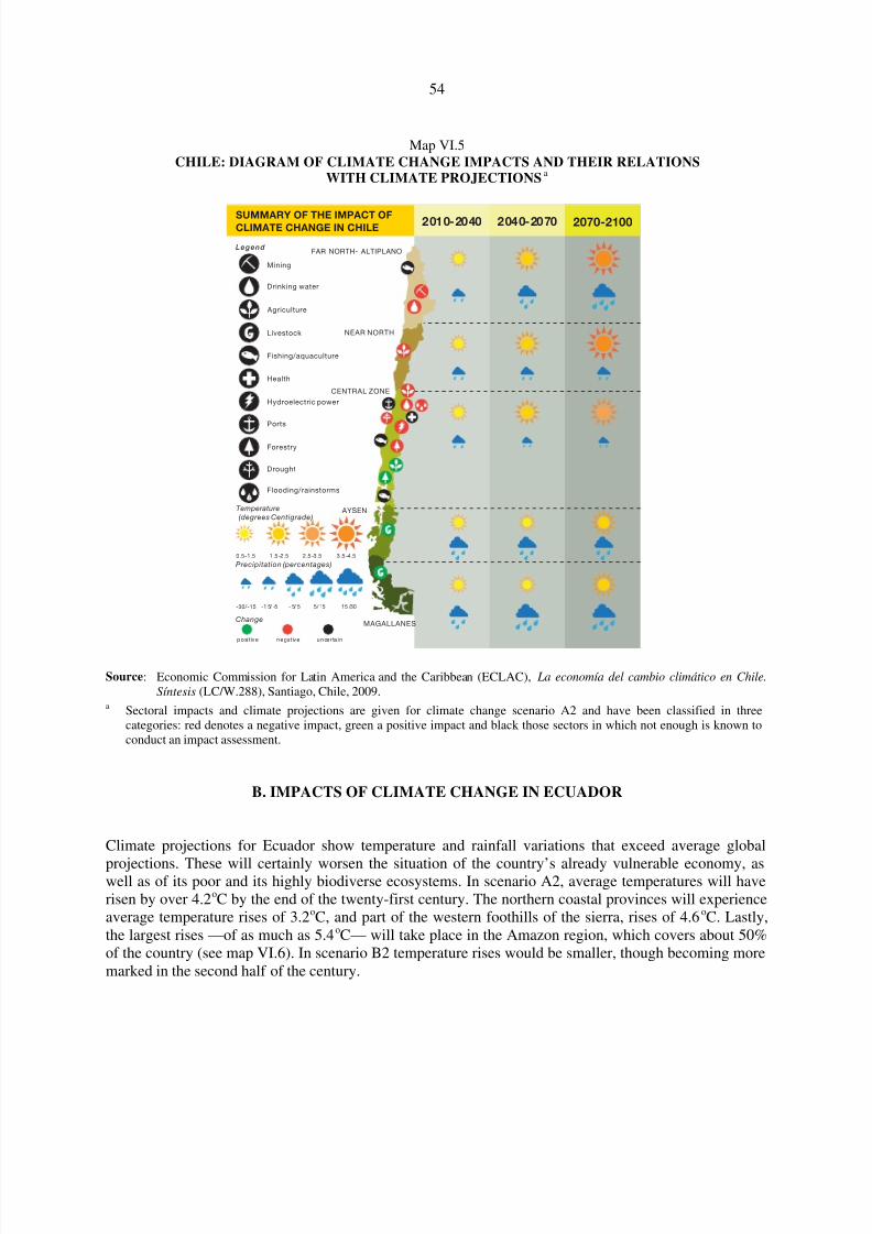
8/8/2019 CEPAL Climate Change 2010
http://slidepdf.com/reader/full/cepal-climate-change-2010 54/107
54
Map VI.5
CHILE: DIAGRAM OF CLIMATE CHANGE IMPACTS AND THEIR RELATIONSWITH CLIMATE PROJECTIONS
a
Source: Economic Commission for Latin America and the Caribbean (ECLAC), La economía del cambio climático en Chile.Síntesis (LC/W.288), Santiago, Chile, 2009.
a Sectoral impacts and climate projections are given for climate change scenario A2 and have been classified in threecategories: red denotes a negative impact, green a positive impact and black those sectors in which not enough is known toconduct an impact assessment.
B. IMPACTS OF CLIMATE CHANGE IN ECUADOR
Climate projections for Ecuador show temperature and rainfall variations that exceed average global
projections. These will certainly worsen the situation of the country’s already vulnerable economy, aswell as of its poor and its highly biodiverse ecosystems. In scenario A2, average temperatures will haverisen by over 4.2oC by the end of the twenty-first century. The northern coastal provinces will experienceaverage temperature rises of 3.2oC, and part of the western foothills of the sierra, rises of 4.6oC. Lastly,the largest rises —of as much as 5.4oC— will take place in the Amazon region, which covers about 50%of the country (see map VI.6). In scenario B2 temperature rises would be smaller, though becoming moremarked in the second half of the century.
SUMMARY OF THE IMPACT OFCLIMATE CHANGE IN CHILE
2010-2040 2040-2070 2070-2100
FAR NORTH- ALTIPLANO
NEAR NORTH
CENTRAL ZONE
AYSEN
MAGALLANES
Legend
Temperature
(degrees Centigrade)
0.5-1.5
posi t ive negative uncerta in
-30/-15 -1 5/ -5 - 5/ 5 5/ 15 15 /30
1 .5 -2 .5 2 .5 -3 .5 3 .5 -4 .5
Precipitation (percentages)
Change
Mining
Drinking water
Agriculture
Hydroelectric power
Health
Ports
Forestry
Fishing/aquaculture
Livestock
Drought
Flooding/rainstorms

8/8/2019 CEPAL Climate Change 2010
http://slidepdf.com/reader/full/cepal-climate-change-2010 55/107

8/8/2019 CEPAL Climate Change 2010
http://slidepdf.com/reader/full/cepal-climate-change-2010 56/107
56
Map VI.7ECUADOR: CHANGE IN PRECIPITATION WITH RESPECT TO THE
BASELINE IN SCENARIO A2, 2100(Millimetres per day)
Source: Economic Commission for Latin America and the Caribbean (ECLAC), on the basis of the PRECIS model.
Some of the physical and economic impacts of temperature and rainfall variations will reduceagricultural productivity in some parts of the country, damage major infrastructure works, cause majorlosses in biodiversity and carbon storage capacity, reduce the water supply and increase water demand,and drive an expansion of vector-borne epidemics. The rise in average sea levels will weaken thecapability of Ecuador’s coastal ecosystems to supply environmental services. In a unique ecosystem suchas the Galapagos Islands, the rise in sea level will have serious implications for some species.
Ecuador has a surplus supply of water resources, which will vary from 42.5 hm3 to 50.7 hm3 by2100, depending on the climate change scenario prevailing globally at that time. This balance is notevenly distributed throughout the country, however; there are differences by type of area. Higher rainfallon the northern coast could generate supply beyond the needs of economic uses. The southern and central
coastal areas, meanwhile, may come under permanent threat of water stress, the first owing to reducedsupply and the second to increased demand. The central sierra may also be exposed to intermediate levelsof water stress. This situation of overall surplus, but with areas under permanent threat of water stress,will pose massive challenges for public policy as regards territorial management.
Provincial boundary
-2 − -0.85 Mm/day
-0.84 − -0.19 Mm/day
-0.18 − 0.3 Mm/day
0.31 − 0.61 Mm/day
0.62 − 0.93 Mm/day
0.94 − 1.4 Mm/day
1.5 − 1.9 Mm/day
2 − 2.4 Mm/day
2.5 − 2.9 Mm/day
3 − 3.5 Mm/day
3.6 − 4.2 Mm/day
4.3 − 5.4 Mm/day
Variation
8/8/2019 CEPAL Climate Change 2010
http://slidepdf.com/reader/full/cepal-climate-change-2010 57/107
57
In this context, meeting rising net demand for water could represent an additional cost equivalentto US$ 47.6 million per year in the last decade of the twenty-first century. On average, the sierra wouldrepresent 60% of the losses during that period (rising gradually towards 2100), followed by the coast with38%, while costs would be marginal in the Amazon region.
Rising temperatures and rainfall will drive productivity gains in the agricultural sector up tocertain thresholds, after which yields begin to fall. By 2100, the end of the analysis period, yields of durum maize will rise by as much as 36%, and of rice by 37%, in scenario A2. All the other cropsexamined will register productivity losses. In the cases of soft maize and beans, which are grown mainlyby small farmers in the sierra, these losses (53% and 9%, respectively) could have food securityimplications. Bananas, sugarcane, coffee and cacao also show heavy losses (of 41%, 36%, 23% and 21%,respectively).
Analysis of production units by technology type suggests that subsistence farming taking place athigher altitudes and in suboptimal production temperatures could benefit from the temperature risesprojected. In intermediate units working in temperatures above the optimum production temperature,
output will fall for most crops, with the exception of rice and durum maize. Lastly, corporate agriculture,which produces mainly for export, will see the largest output declines. Overall, in scenario A2 theagricultural sector will post net losses of as much as US$ 254 million per year during the last decade of the century.
Because of their geographical location and altitudinal thresholds, Ecuador’s ecosystems areamong the most megadiverse in the world and boast some of the greatest concentrations of species inrelation to surface area in South America. Yet 2,208 species are included in different threat categories(IUCN, 2008). This natural endowment offers a number of important environmental services for thecountry, which has made major efforts to protect them. Ecuador has 40 protected natural areas, coveringan area of about 4 million hectares, or 19% of the country’s total area, distributed between the coast, thesierra, the Amazon region and the Galapagos Islands (see map VI.8).
In 2091-2100, climate change will affect mainly the cloud forest, which shows a reduction in areaof over 80% in both scenarios, while the surface area of evergreen forest will decrease by around 70%.Low-altitude forests and paramo areas will sustain only slight alternations. The loss of plant speciesthrough the alteration or replacement of plant formations will cause the extinction of numerous animalspecies owing to the disappearance of the ecosystem structures needed to segregate habitats or formniches, which must have the food, rest, nesting and shelter resources for different animals species. Theloss or transformation of continental natural ecosystems will also generate voluminous CO2 emissions.
Marine and coastal habitats in Ecuador are of continental origin, formed by constantly changingsediment deposits brought to the ocean by rivers. The result is a broad ocean platform and wetlands alongthe coast of Ecuador. The alteration of climate variables that affect the coastline would create a complex
situation, and would be likely to cause reduction in cloud cover, a 35% increase in precipitation and, as aresult, substantial increases in fresh water flows in river mouths and a rise of up to half a metre in averagesea levels. Among other multiple effects, this would cause damage to coastal species and habitats,regression of mangrove roots, replacement and loss of up to 40% of beach area in provinces such asEsmeraldas and El Oro, flooding of 191,000 hectares of arable land, and loss of economically importantbottom species, up to 22% of whose mangrove habitats will be compromised. All this will generate apartial economic cost of about US$ 45.6 million per year during the last decade of the century in lossesfrom tourism and sectors harvesting shrimp and bottom fish.

8/8/2019 CEPAL Climate Change 2010
http://slidepdf.com/reader/full/cepal-climate-change-2010 58/107
58
Map VI.8ECUADOR: PLANT FORMATIONS IN PROTECTED NATURAL AREAS
Source: Ministry of the Environment of Ecuador, National System of Protected Areas.
The Galapagos Islands are located 1,050 km from the coast of Ecuador in the Pacific Ocean. Theyconsist of 13 volcanic islands, 6 smaller islands and 107 rocks and islets. Ninety-seven per cent of theislands’ area is classified as protected as a national park. The Galapagos Islands are important since theypossess a high level of endemic species, have great aesthetic value and form part of the UNESCO WorldHeritage List. The effects of climate change are likely to change their ecosystemic zoning. The maineconomic impact is thought to be associated with the loss of income from scientific research, the intrinsicvalue of the ecosystems and the species that inhabit them, as well as the value of present and potentialusage of this unique ecosystem, principally for tourism. Economic activity in the Galapagos Islandsrepresented 0.49% of Ecuador’s total GDP in 2000-2006, and tourism and related activities represent 82%of the gross output of Galapagos. In light of this, the economic cost of climate change from tourism sectorlosses, in a scenario of a 1-metre rise in average sea levels, could be as much as US$ 25 million per yearin the last decade of the century.
Malaria and dengue fever are public health problems. Their cycles shift from endemic toepidemic, influenced by factors environmental (weather phenomena), socioeconomic and cultural. Theybring death and disease and have severe social and economic repercussions, particularly for the poorerpopulations in the tropical and subtropical areas that make up around 70% of the country.
Mangrove
Manglillo
Tidal evergreen forest (guandal)
Evergreen forest of the coastal mountain foothills
Evergreen forest of the coastal lower montane belt
Cloud forest of the coastal lower montane belt
Coastal lowland evergreen forest
Coastal foothills evergreen forest
Coastal lowland deciduous forest
Coastal foothills deciduous forest
Coastal lowland semideciduous forest
Coastal foothills semideciduous forest
Western Andes lower montane belt evergreen forest
Western Andes upper montane belt evergreen forest
Western Andes montane cloud forest
Western Andes lower montane semideciduous forest
Coastal lowland dry scrub
Shrub savannah
Lowland grassland
Southern Andes dry montane shrubland
Northern and Central Andes dry montane shrubland
Low montane dry shrubland
Southern Andes wet shrubland
Northern and Central Andes wet shrubland
Upper montane grasslandMontane grassland
Dry paramo
Herbaceous paramo
Southern Andes shrub paramo
Frailejones paramo
Almohadillas paramo
Superparamo
Permanent snow
Amazon lowlands evergreen forest
Amazon lower montane evergreen forest
South-eastern Andes lower montane evergreen forest
Eastern Andes upper montane evergreen forest
Amazon montane evergreen forest
Evergreen forest of the Amazon foothills
Eastern Andes lower montane evergreen forest
Palmas and Aguas Negras lowland forest
Aguas Negras lowland tidal forest
Eastern Andes cloud forest
Amazon montane wet scrubland
Amazon upper montane wet scrubland
Amazon lowland grasslands
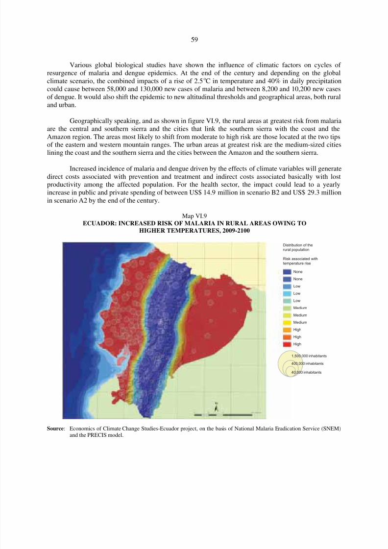
8/8/2019 CEPAL Climate Change 2010
http://slidepdf.com/reader/full/cepal-climate-change-2010 59/107
59
Various global biological studies have shown the influence of climatic factors on cycles of resurgence of malaria and dengue epidemics. At the end of the century and depending on the globalclimate scenario, the combined impacts of a rise of 2.5oC in temperature and 40% in daily precipitationcould cause between 58,000 and 130,000 new cases of malaria and between 8,200 and 10,200 new cases
of dengue. It would also shift the epidemic to new altitudinal thresholds and geographical areas, both ruraland urban.
Geographically speaking, and as shown in figure VI.9, the rural areas at greatest risk from malariaare the central and southern sierra and the cities that link the southern sierra with the coast and theAmazon region. The areas most likely to shift from moderate to high risk are those located at the two tipsof the eastern and western mountain ranges. The urban areas at greatest risk are the medium-sized citieslining the coast and the southern sierra and the cities between the Amazon and the southern sierra.
Increased incidence of malaria and dengue driven by the effects of climate variables will generatedirect costs associated with prevention and treatment and indirect costs associated basically with lostproductivity among the affected population. For the health sector, the impact could lead to a yearly
increase in public and private spending of between US$ 14.9 million in scenario B2 and US$ 29.3 millionin scenario A2 by the end of the century.
Map VI.9ECUADOR: INCREASED RISK OF MALARIA IN RURAL AREAS OWING TO
HIGHER TEMPERATURES, 2009-2100
Source: Economics of Climate Change Studies-Ecuador project, on the basis of National Malaria Eradication Service (SNEM)and the PRECIS model.
None
None
Low
Low
Low
Medium
Medium
Medium
High
High
High
Distribution of the
rural population
Risk associated with
temperature rise
1,500,000 inhabitants
400,000 inhabitants
40,000 inhabitants
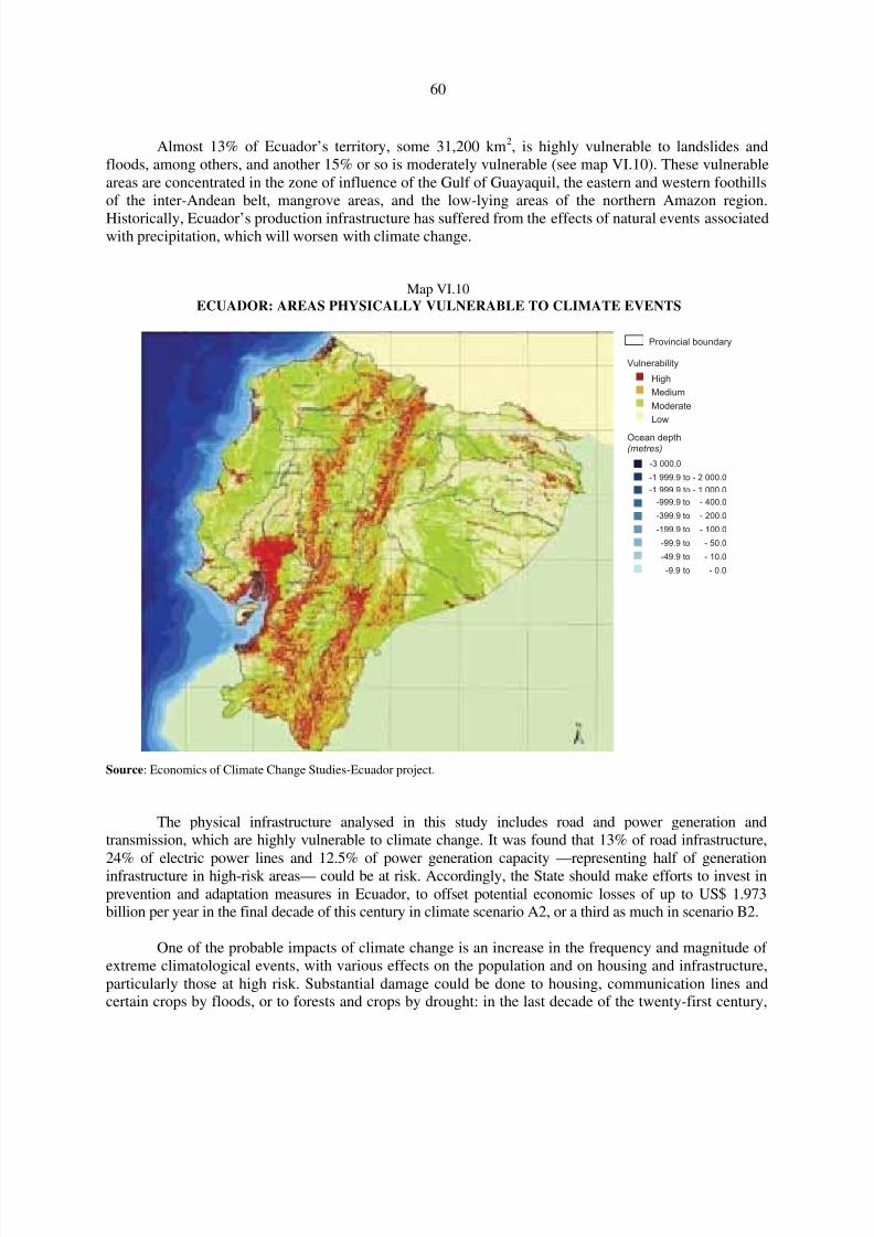
8/8/2019 CEPAL Climate Change 2010
http://slidepdf.com/reader/full/cepal-climate-change-2010 60/107
60
Almost 13% of Ecuador’s territory, some 31,200 km2, is highly vulnerable to landslides andfloods, among others, and another 15% or so is moderately vulnerable (see map VI.10). These vulnerableareas are concentrated in the zone of influence of the Gulf of Guayaquil, the eastern and western foothillsof the inter-Andean belt, mangrove areas, and the low-lying areas of the northern Amazon region.
Historically, Ecuador’s production infrastructure has suffered from the effects of natural events associatedwith precipitation, which will worsen with climate change.
Map VI.10ECUADOR: AREAS PHYSICALLY VULNERABLE TO CLIMATE EVENTS
Source: Economics of Climate Change Studies-Ecuador project.
The physical infrastructure analysed in this study includes road and power generation andtransmission, which are highly vulnerable to climate change. It was found that 13% of road infrastructure,24% of electric power lines and 12.5% of power generation capacity —representing half of generationinfrastructure in high-risk areas— could be at risk. Accordingly, the State should make efforts to invest inprevention and adaptation measures in Ecuador, to offset potential economic losses of up to US$ 1.973billion per year in the final decade of this century in climate scenario A2, or a third as much in scenario B2.
One of the probable impacts of climate change is an increase in the frequency and magnitude of extreme climatological events, with various effects on the population and on housing and infrastructure,particularly those at high risk. Substantial damage could be done to housing, communication lines andcertain crops by floods, or to forests and crops by drought: in the last decade of the twenty-first century,
Vulnerability
High
Medium
Moderate
Low
Ocean depth(metres)
-1 999.9 to - 1 000.0
-999.9 to - 400.0
-399.9 to - 200.0
-199.9 to - 100.0
-99.9 to - 50.0
-49.9 to - 10.0
-9.9 to - 0.0
-3 000.0
Provincial boundary
-1 999.9 to - 2 000.0

8/8/2019 CEPAL Climate Change 2010
http://slidepdf.com/reader/full/cepal-climate-change-2010 61/107
61
in climate scenario A2, 221,000 dwellings could be damaged or lost and almost 1.3 million hectares of cropland or forestry could suffer from excess or lack of precipitation.
The economic impact of extreme events associated with climate change —those additional to
what would be expected in normal conditions— will be perceptible as of the 2050s, when the negativeimpact could be US$ 413 million current dollars. In the last decade of the century, the damage willincrease to some US$ 1.56 billion per year.
Overall, the economic assessment of climate change impacts on the different sectors analysedgives a negative net balance for Ecuador. By the end of the century the annual costs could vary betweenUS$ 1.35 billion and US$ 2.7 billion in current figures, depending on the global emissions scenarioprevailing, B2 o A2, which could mean an annual loss of 2% of GDP for the last decade. These costs arein addition to the loss of biodiversity and ecosystems and the additional extreme events caused by climatechange, which could swell the figures considerably, particularly in scenario A2. Although all these figuresmust be treated with extreme caution, given the uncertainty associated with climate and economicprojections, the lack of knowledge of numerous impacts, and methodological limitations, the aggregate
impacts could represent several times current GDP at a 0.5% discount rate. Without doubt, policystrategies for reducing vulnerability to the impacts of climate change must make it a priority to identifyadaptation measures and the means to finance them.
C. IMPACTS OF CLIMATE CHANGE IN URUGUAY
The characteristics of the Uruguayan territory are highly relevant to the analysis of climate change. Theentire country is temperate and humid with irregular precipitation, average temperatures and no dryseason. Precipitation is generally liquid, only occasionally in the solid form of hail or snow, and highlyvariable.
In the A2 scenario, a temperature rise of just over 3ºC is projected for Uruguay by the end of theperiod. In the B2 scenario, the rise is slightly smaller. In both cases, precipitation is projected to increaseslightly, with greater year-on-year variability (see table VI.2). According to scenarios prepared by theIntergovernmental Panel on Climate Change (IPCC), the main consequences of climate change inUruguay will be greater frequency and intensity of extreme events and a rise in average sea levels.
Table VI.2URUGUAY: ESTIMATES FOR AVERAGE TEMPERATURE AND PRECIPITATION
IN CLIMATE CHANGE SCENARIOS A2 AND B2
Average temperature
(Degrees Centigrade)
Average precipitation
(Millimetres per day) Year Scenario A2 Scenario B2 Year Scenario A2 Scenario B2
2006 17.64 17.64 2006 3.41 3.41
2030 18.91 18.35 2030 3.41 3.51
2050 18.88 18.88 2050 3.43 3.52
2070 19.69 19.31 2070 3.45 3.56
2100 20.71 19.96 2100 3.63 3.70
Source: Economic Commission for Latin America and the Caribbean (ECLAC), “La economía del cambio climático enUruguay. Síntesis”, Project documents, No. 330 (LC/W.330), Santiago, Chile, 2010.

8/8/2019 CEPAL Climate Change 2010
http://slidepdf.com/reader/full/cepal-climate-change-2010 62/107
62
Climate change scenarios were used to analyse possible economic impacts in Uruguay. Twosocioeconomic scenarios were formulated for 2100, on the basis of those prepared by the Office of Planning and the Budget (OPP) for the strategy known as “Uruguay III Century”, which assume buoyantsocioeconomic growth and extensive use of natural resources, on the one hand, and more modest
economic growth and more careful use of natural resources, on the other. The two socioeconomicscenarios were used to prepare the different sectoral studies by factoring in climate change impacts (A2and B2 scenarios, respectively).
With respect to water resources, the study showed demand rising, but without threatening thecapacity of the different water basins, except for Lake Merin, which supplies water for rice irrigation. Theprojected increase in drinking water demand between 2006 and 2100 without climate change (86%)would be 5 percentage points larger in the A2 climate change scenario. Water demand would rise by 0.4%annually in the more conservative socioeconomic scenario, with climate change (B2) again producing anincrease of about 5 percentage points. The impact of higher temperatures on drinking water demandshows a fairly significant adverse economic impact.
For the energy sector, demand scenarios were analysed for 2030 using an international modeladopted for Uruguay. Results were then extrapolated to 2100 on the basis of socioeconomic scenarios andfuture energy intensity assumptions, using an econometric model to incorporate the impacts of climatechange. The energy sources that would be used to meet additional demand were then defined, taking intoaccount the fact that, with no capacity to increase the hydroelectric power supply, it would be necessaryto resort to thermal sources. A reference value of US$ 70 per barrel of petroleum was assumed to quantifythe economic impact of climate-driven rises in energy demand. This gave a significant cumulativeadditional expenditure up to 2100: US$ 3.722 billion using a discount rate of 4% per year for the high-growth scenario combined with A2 climate change, and US$ 2.283 billion for the low-growth scenariocombined with B2 climate change.
The agriculture sector is likely to benefit from increased yields owing to higher temperatures up
to a certain point, at which the process will go into reverse. Accordingly, in the A2 climate changescenario, the agricultural sector will gain in the next few decades but sustain adverse impacts in thesecond half of the century. In the B2 scenario, the outcomes will be positive for agriculture throughout thecentury, providing that the sector uses techniques which avoid degrading or desertifying land as theagricultural frontier expands, as the hypothesis suggests it will (see table VI.3).
Table VI.3URUGUAY: IMPACT OF CLIMATE CHANGE ON GROSS VALUE OF PRODUCTION AND
AGRICULTURAL GDP BY SCENARIO, 2007-2100(Millions of dollars at constant 2007 prices)
2030 2050 2070 2100
A2 B2 A2 B2 A2 B2 A2 B2Cereals and oilseeds 185 92 -194 169 -284 169 -508 169
Animal products 174 136 -80 182 -160 182 -287 182
Forestry products 15 6 39 13 52 18 19 18
Gross value of production 374 233 -235 364 -392 368 -775 368
GDP 229 152 -128 227 -224 229 -441 229
Source: Economic Commission for Latin America and the Caribbean (ECLAC), “La economía del cambio climático enUruguay. Síntesis”, Project documents, No. 330 (LC/W.330), Santiago, Chile, 2010.
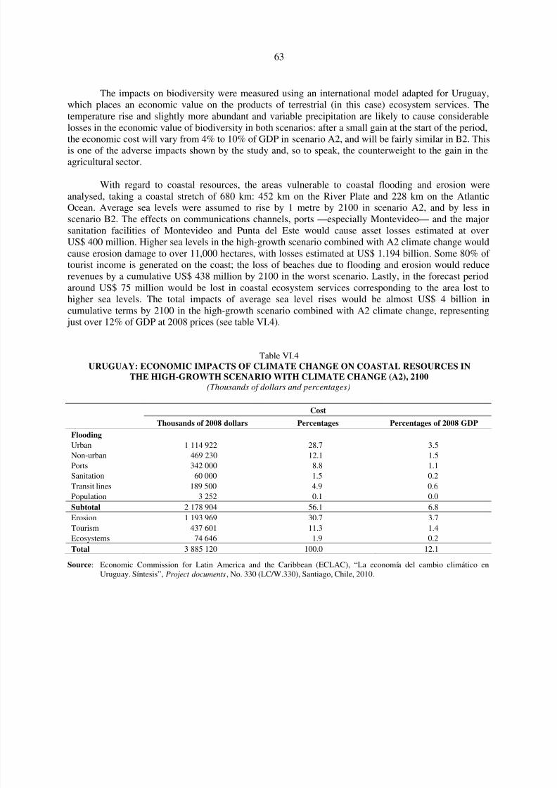
8/8/2019 CEPAL Climate Change 2010
http://slidepdf.com/reader/full/cepal-climate-change-2010 63/107
63
The impacts on biodiversity were measured using an international model adapted for Uruguay,which places an economic value on the products of terrestrial (in this case) ecosystem services. Thetemperature rise and slightly more abundant and variable precipitation are likely to cause considerablelosses in the economic value of biodiversity in both scenarios: after a small gain at the start of the period,
the economic cost will vary from 4% to 10% of GDP in scenario A2, and will be fairly similar in B2. Thisis one of the adverse impacts shown by the study and, so to speak, the counterweight to the gain in theagricultural sector.
With regard to coastal resources, the areas vulnerable to coastal flooding and erosion wereanalysed, taking a coastal stretch of 680 km: 452 km on the River Plate and 228 km on the AtlanticOcean. Average sea levels were assumed to rise by 1 metre by 2100 in scenario A2, and by less inscenario B2. The effects on communications channels, ports —especially Montevideo— and the majorsanitation facilities of Montevideo and Punta del Este would cause asset losses estimated at overUS$ 400 million. Higher sea levels in the high-growth scenario combined with A2 climate change wouldcause erosion damage to over 11,000 hectares, with losses estimated at US$ 1.194 billion. Some 80% of tourist income is generated on the coast; the loss of beaches due to flooding and erosion would reduce
revenues by a cumulative US$ 438 million by 2100 in the worst scenario. Lastly, in the forecast periodaround US$ 75 million would be lost in coastal ecosystem services corresponding to the area lost tohigher sea levels. The total impacts of average sea level rises would be almost US$ 4 billion incumulative terms by 2100 in the high-growth scenario combined with A2 climate change, representing just over 12% of GDP at 2008 prices (see table VI.4).
Table VI.4URUGUAY: ECONOMIC IMPACTS OF CLIMATE CHANGE ON COASTAL RESOURCES IN
THE HIGH-GROWTH SCENARIO WITH CLIMATE CHANGE (A2), 2100(Thousands of dollars and percentages)
CostThousands of 2008 dollars Percentages Percentages of 2008 GDP
Flooding
Urban 1 114 922 28.7 3.5
Non-urban 469 230 12.1 1.5
Ports 342 000 8.8 1.1
Sanitation 60 000 1.5 0.2
Transit lines 189 500 4.9 0.6
Population 3 252 0.1 0.0
Subtotal 2 178 904 56.1 6.8
Erosion 1 193 969 30.7 3.7
Tourism 437 601 11.3 1.4
Ecosystems 74 646 1.9 0.2
Total 3 885 120 100.0 12.1Source: Economic Commission for Latin America and the Caribbean (ECLAC), “La economía del cambio climático en
Uruguay. Síntesis”, Project documents, No. 330 (LC/W.330), Santiago, Chile, 2010.
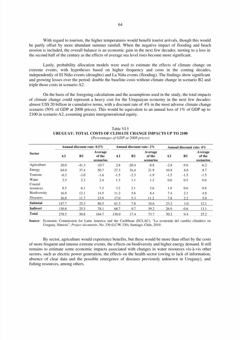
8/8/2019 CEPAL Climate Change 2010
http://slidepdf.com/reader/full/cepal-climate-change-2010 64/107
64
With regard to tourism, the higher temperatures would benefit tourist arrivals, though this wouldbe partly offset by more abundant summer rainfall. When the negative impact of flooding and beacherosion is included, the overall balance is an economic gain in the next few decades, turning to a loss inthe second half of the century as the effects of average sea level rises become more significant.
Lastly, probability allocation models were used to estimate the effects of climate change onextreme events, with hypotheses based on higher frequency and costs in the coming decades,independently of El Niño events (droughts) and La Niña events (flooding). The findings show significantand growing losses over the period: double the baseline costs without climate change in scenario B2 andtriple those costs in scenario A2.
On the basis of the foregoing calculations and the assumptions used in the study, the total impactsof climate change could represent a heavy cost for the Uruguayan economy in the next few decades:almost US$ 20 billion in cumulative terms, with a discount rate of 4% in the most adverse climate changescenario (50% of GDP at 2008 prices). This would be equivalent to an annual loss of 1% of GDP up to2100 in scenario A2, assuming greater intergenerational equity.
Table VI.5URUGUAY: TOTAL COSTS OF CLIMATE CHANGE IMPACTS UP TO 2100
(Percentages of GDP at 2008 prices)
Sector
Annual discount rate: 0.5% Annual discount rate: 2% Annual discount rate: 4%
A2 B2Average
of the
scenarios
A2 B2Average
of the
scenarios
A2 B2Average
of the
scenarios
Agriculture 20.0 -41.3 -10.7 2.8 -20.4 -8.8 -2.8 -9.6 -6.2
Energy 64.0 37.4 50.7 27.3 16.4 21.9 10.8 6.6 8.7
Tourism -0.3 -3.0 -1.6 -1.5 -2.3 -1.9 -1.5 -1.5 -1.5
Water 2.5 2.3 2.4 1.3 1.1 1.2 0.6 0.5 0.6Coastalresources 8.5 6.1 7.3 3.2 2.1 2.6 1.0 0.6 0.8
Biodiversity 16.9 12.1 14.5 11.2 5.6 8.4 7.4 2.1 4.8
Disasters 36.0 11.7 23.9 17.0 5.3 11.2 7.8 2.2 5.0
Subtotal 147.7 25.3 86.5 61.3 7.8 34.6 23.2 1.0 12.1
Indirect 130.8 25.5 78.1 68.7 9.7 39.2 26.9 -0.6 13.1
Total 278.5 50.8 164.7 130.0 17.4 73.7 50.2 0.4 25.2
Source: Economic Commission for Latin America and the Caribbean (ECLAC), “La economía del cambio climático enUruguay. Síntesis”, Project documents, No. 330 (LC/W.330), Santiago, Chile, 2010.
By sector, agriculture would experience benefits, but these would be more than offset by the costsof more frequent and intense extreme events, the effects on biodiversity and higher energy demand. It stillremains to estimate some economic impacts associated with changes in water resources vis-à-vis othersectors, such as electric power generation, the effects on the health sector (owing to lack of information,absence of clear data and the possible emergence of diseases previously unknown in Uruguay), andfishing resources, among others.
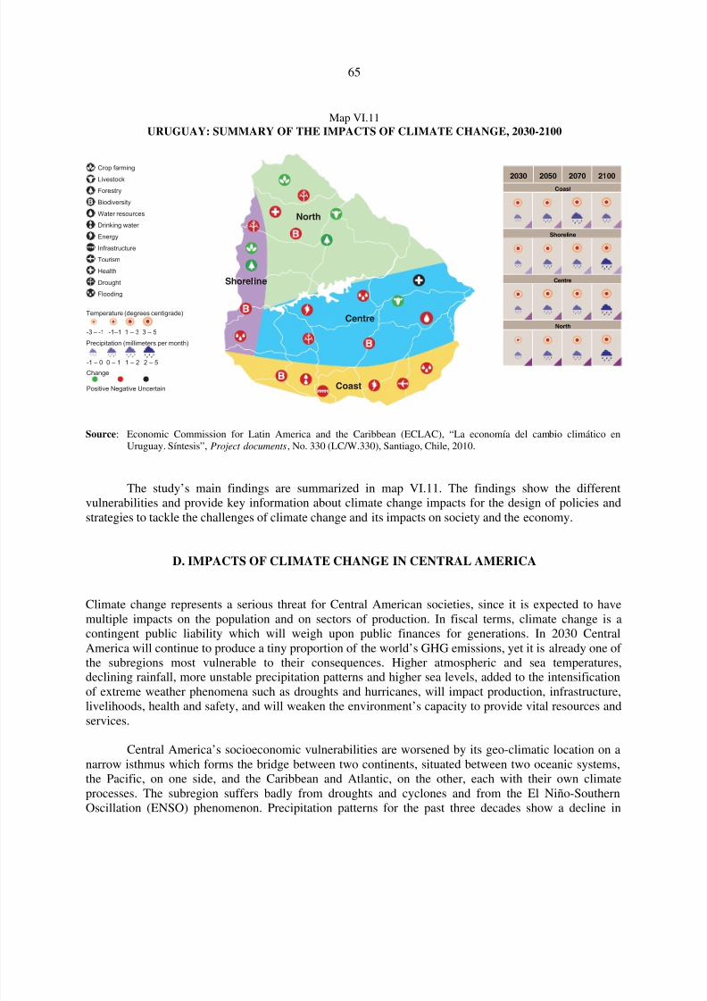
8/8/2019 CEPAL Climate Change 2010
http://slidepdf.com/reader/full/cepal-climate-change-2010 65/107
65
Map VI.11URUGUAY: SUMMARY OF THE IMPACTS OF CLIMATE CHANGE, 2030-2100
Source: Economic Commission for Latin America and the Caribbean (ECLAC), “La economía del cambio climático enUruguay. Síntesis”, Project documents, No. 330 (LC/W.330), Santiago, Chile, 2010.
The study’s main findings are summarized in map VI.11. The findings show the differentvulnerabilities and provide key information about climate change impacts for the design of policies andstrategies to tackle the challenges of climate change and its impacts on society and the economy.
D. IMPACTS OF CLIMATE CHANGE IN CENTRAL AMERICA
Climate change represents a serious threat for Central American societies, since it is expected to havemultiple impacts on the population and on sectors of production. In fiscal terms, climate change is acontingent public liability which will weigh upon public finances for generations. In 2030 CentralAmerica will continue to produce a tiny proportion of the world’s GHG emissions, yet it is already one of the subregions most vulnerable to their consequences. Higher atmospheric and sea temperatures,declining rainfall, more unstable precipitation patterns and higher sea levels, added to the intensificationof extreme weather phenomena such as droughts and hurricanes, will impact production, infrastructure,
livelihoods, health and safety, and will weaken the environment’s capacity to provide vital resources andservices.
Central America’s socioeconomic vulnerabilities are worsened by its geo-climatic location on anarrow isthmus which forms the bridge between two continents, situated between two oceanic systems,the Pacific, on one side, and the Caribbean and Atlantic, on the other, each with their own climateprocesses. The subregion suffers badly from droughts and cyclones and from the El Niño-SouthernOscillation (ENSO) phenomenon. Precipitation patterns for the past three decades show a decline in
2030 2050 2070 2100
Temperature (degrees centigrade)
Precipitation (millimeters per month)
Change
Positive Negative Uncertain
2 – 51 – 20 – 1-1 – 0
3 – 51 – 3-1–1-3 – -1
Coast
Shoreline
Centre
North
North
Shoreline
Centre
Coast
Crop farming
Livestock
Forestry
Biodiversity
Water resources
Drinking water
Energy
Infrastructure
Tourism
Health
Drought
Flooding

8/8/2019 CEPAL Climate Change 2010
http://slidepdf.com/reader/full/cepal-climate-change-2010 66/107
66
rainfall, especially in the western part of Central America, and a temperature rise of between 0.7°C and1°C. Since climate-driven factors contribute heavily to economic activities, especially agriculture, theimpact of climate change on the subregion’s economy will increase throughout this century. CentralAmerica also possesses valuable ecosystems with abundant biodiversity, including forests, coral reefs and
mangroves, which provide multiple services to the population. The existing unsustainable pattern of development is already taking a toll on these ecosystems —some of which are already severelydegraded— and climate change will only worsen these effects.
On the basis of three predictive models and in a conservative emissions scenario (B2),temperatures will rise by between 2.2°C and 2.7°C by 2100, depending on the country, with an averageregional jump of 2.5°C over the average for 1980-2000. In scenario A2, temperatures may rise bybetween 3.6°C and 4.7° C, depending on the country, with an average regional increase of 4.2°C. Thetrajectory of precipitation levels is more uncertain and shows greater differences between countries.Central America’s average precipitation is expected to decline by 11% by 2100 in the B2 globalemissions scenario, and by 28% in the A2 scenario.
Climate-change-sensitive sectors and activities were assessed taking into account climateoutcomes and trend scenarios for economic growth, population and land use change. The sectors chosenare examined in relation to the impacts of extreme events, the availability of water resources, the impactson the agricultural sector and biodiversity.
Between 1930 and 2008, Central America recorded 248 major extreme events associated withweather phenomena. There is also evidence of multiple smaller events, whose cumulative impacts havenot been assessed. The most frequent events are floods and flash floods, storms and landslides, accountingfor 85%, followed by droughts, which account for 9%.
Figure VI.1
CENTRAL AMERICA: MAIN EXTREME WEATHER EVENTS, 1970-2008(Number of events recorded)
Source: Economic Commission for Latin America and the Caribbean (ECLAC), on the basis of Regional Disaster InformationCenter (CRID), 2010, Emergency Events Database (EM-DATA) [online] http://www.emdat.be/Database/terms.html.
Bel ize Costa Rica El Salvador Guatemala
1970-1989 1990-2008 1970-1989 1990-2008
20
18
16
14
12
10
8
6
4
2
0
16
14
12
10
8
6
4
2
0
PanamaNicaraguaHonduras Belize Costa Rica El Salvador Guatemala PanamaNicaraguaHonduras
A. Floods B. Tropical storms and hurricanes
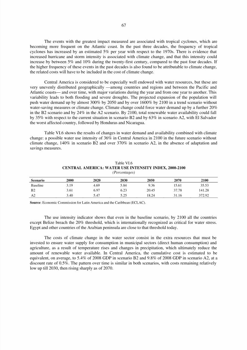
8/8/2019 CEPAL Climate Change 2010
http://slidepdf.com/reader/full/cepal-climate-change-2010 67/107
67
The events with the greatest impact measured are associated with tropical cyclones, which arebecoming more frequent on the Atlantic coast. In the past three decades, the frequency of tropicalcyclones has increased by an estimated 5% per year with respect to the 1970s. There is evidence thatincreased hurricane and storm intensity is associated with climate change, and that this intensity could
increase by between 5% and 10% during the twenty-first century, compared to the past four decades. If the higher frequency of these events in the past decades is also found to be attributable to climate change,the related costs will have to be included in the cost of climate change.
Central America is considered to be especially well endowed with water resources, but these arevery unevenly distributed geographically —among countries and regions and between the Pacific andAtlantic coasts— and over time, with major variations during the year and from one year to another. Thisvariability leads to both flooding and severe droughts. The projected expansion of the population willpush water demand up by almost 300% by 2050 and by over 1600% by 2100 in a trend scenario withoutwater-saving measures or climate change. Climate change could force water demand up by a further 20%in the B2 scenario and by 24% in the A2 scenario. By 2100, total renewable water availability could fallby 35% with respect to the current situation in scenario B2 and by 63% in scenario A2, with El Salvador
the worst affected country, followed by Honduras and Nicaragua.
Table VI.6 shows the results of changes in water demand and availability combined with climatechange: a possible water use intensity of 36% in Central America in 2100 in the future scenario withoutclimate change, 140% in scenario B2 and over 370% in scenario A2, in the absence of adaptation andsavings measures.
Table VI.6CENTRAL AMERICA: WATER USE INTENSITY INDEX, 2000-2100
(Percentages)
Scenario 2000 2020 2030 2050 2070 2100
Baseline 3.19 4.69 5.84 9.36 15.61 35.53
B2 3.61 6.97 6.23 20.45 37.78 141.28
A2 3.40 5.47 5.25 18.24 31.16 372.92
Source: Economic Commission for Latin America and the Caribbean (ECLAC).
The use intensity indicator shows that even in the baseline scenario, by 2100 all the countriesexcept Belize breach the 20% threshold, which is internationally recognized as critical for water stress.Egypt and other countries of the Arabian peninsula are close to that threshold today.
The costs of climate change in the water sector consist in the extra resources that must beinvested to ensure water supply for consumption in municipal sectors (direct human consumption) andagriculture, as a result of temperature rises and changes in precipitation, which ultimately reduce theamount of renewable water available. In Central America, the cumulative cost is estimated to beequivalent, on average, to 5.4% of 2008 GDP in scenario B2 and 9.8% of 2008 GDP in scenario A2, at adiscount rate of 0.5%. The pattern over time is similar in both scenarios, with costs remaining relativelylow up till 2030, then rising sharply as of 2070.
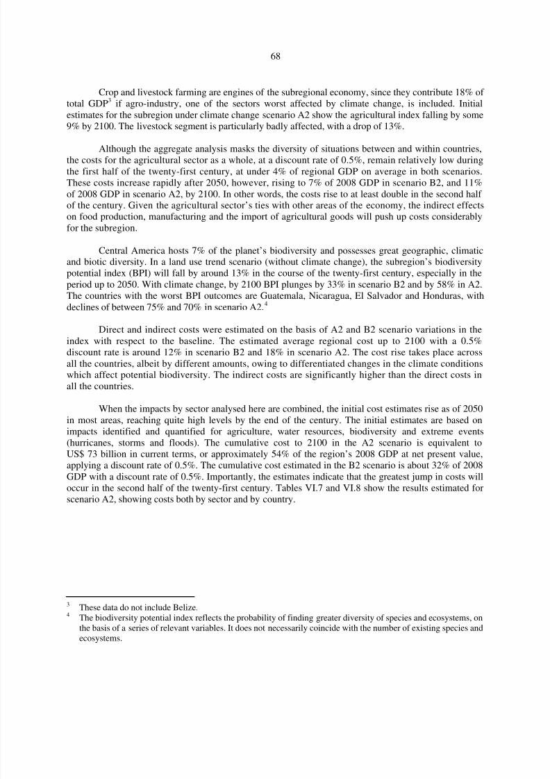
8/8/2019 CEPAL Climate Change 2010
http://slidepdf.com/reader/full/cepal-climate-change-2010 68/107
68
Crop and livestock farming are engines of the subregional economy, since they contribute 18% of total GDP3 if agro-industry, one of the sectors worst affected by climate change, is included. Initialestimates for the subregion under climate change scenario A2 show the agricultural index falling by some9% by 2100. The livestock segment is particularly badly affected, with a drop of 13%.
Although the aggregate analysis masks the diversity of situations between and within countries,the costs for the agricultural sector as a whole, at a discount rate of 0.5%, remain relatively low duringthe first half of the twenty-first century, at under 4% of regional GDP on average in both scenarios.These costs increase rapidly after 2050, however, rising to 7% of 2008 GDP in scenario B2, and 11%of 2008 GDP in scenario A2, by 2100. In other words, the costs rise to at least double in the second half of the century. Given the agricultural sector’s ties with other areas of the economy, the indirect effectson food production, manufacturing and the import of agricultural goods will push up costs considerablyfor the subregion.
Central America hosts 7% of the planet’s biodiversity and possesses great geographic, climaticand biotic diversity. In a land use trend scenario (without climate change), the subregion’s biodiversity
potential index (BPI) will fall by around 13% in the course of the twenty-first century, especially in theperiod up to 2050. With climate change, by 2100 BPI plunges by 33% in scenario B2 and by 58% in A2.The countries with the worst BPI outcomes are Guatemala, Nicaragua, El Salvador and Honduras, withdeclines of between 75% and 70% in scenario A2.4
Direct and indirect costs were estimated on the basis of A2 and B2 scenario variations in theindex with respect to the baseline. The estimated average regional cost up to 2100 with a 0.5%discount rate is around 12% in scenario B2 and 18% in scenario A2. The cost rise takes place acrossall the countries, albeit by different amounts, owing to differentiated changes in the climate conditionswhich affect potential biodiversity. The indirect costs are significantly higher than the direct costs inall the countries.
When the impacts by sector analysed here are combined, the initial cost estimates rise as of 2050in most areas, reaching quite high levels by the end of the century. The initial estimates are based onimpacts identified and quantified for agriculture, water resources, biodiversity and extreme events(hurricanes, storms and floods). The cumulative cost to 2100 in the A2 scenario is equivalent toUS$ 73 billion in current terms, or approximately 54% of the region’s 2008 GDP at net present value,applying a discount rate of 0.5%. The cumulative cost estimated in the B2 scenario is about 32% of 2008GDP with a discount rate of 0.5%. Importantly, the estimates indicate that the greatest jump in costs willoccur in the second half of the twenty-first century. Tables VI.7 and VI.8 show the results estimated forscenario A2, showing costs both by sector and by country.
3 These data do not include Belize.4 The biodiversity potential index reflects the probability of finding greater diversity of species and ecosystems, on
the basis of a series of relevant variables. It does not necessarily coincide with the number of existing species andecosystems.
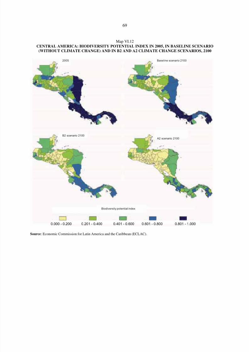
8/8/2019 CEPAL Climate Change 2010
http://slidepdf.com/reader/full/cepal-climate-change-2010 69/107
69
Map VI.12
CENTRAL AMERICA: BIODIVERSITY POTENTIAL INDEX IN 2005, IN BASELINE SCENARIO
(WITHOUT CLIMATE CHANGE) AND IN B2 AND A2 CLIMATE CHANGE SCENARIOS, 2100
Source: Economic Commission for Latin America and the Caribbean (ECLAC).
Biodiversity potential index
A2 scenario 2100
2005 Baseline scenario 2100
B2 scenario 2100
0.000 - 0.200 0.201 - 0.400 0.401 - 0.600 0.601 - 0.800 0.801 - 1.000
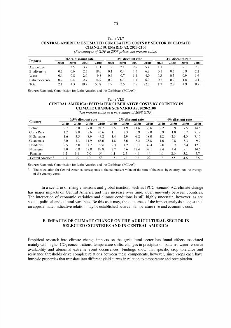
8/8/2019 CEPAL Climate Change 2010
http://slidepdf.com/reader/full/cepal-climate-change-2010 70/107
70
Table VI.7
CENTRAL AMERICA: ESTIMATED CUMULATIVE COSTS BY SECTOR IN CLIMATE
CHANGE SCENARIO A2, 2020-2100(Percentages of GDP at 2008 prices, net present value)
Impacts 0.5% discount rate 2% discount rate 4% discount rate
2020 2030 2050 2100 2020 2030 2050 2100 2020 2030 2050 2100
Agriculture 1.3 2.5 3.7 11.1 1.2 2.1 2.9 5.4 1.1 1.8 2.1 2.8
Biodiversity 0.2 0.6 2.3 18.0 0.1 0.4 1.5 6.8 0.1 0.3 0.9 2.2
Water 0.4 0.8 2.0 9.8 0.4 0.7 1.4 4.0 0.3 0.5 0.9 1.6
Extreme events 0.2 0.4 2.7 14.9 0.2 0.3 1.7 6.0 0.2 0.2 1.0 2.1
Total 2.1 4.3 10.7 53.8 1.9 3.5 7.5 22.2 1.7 2.8 4.9 8.7
Source: Economic Commission for Latin America and the Caribbean (ECLAC).
Table VI.8
CENTRAL AMERICA: ESTIMATED CUMULATIVE COSTS BY COUNTRY IN
CLIMATE CHANGE SCENARIO A2, 2020-2100(Net present value as a percentage of 2008 GDP)
Country 0.5% discount rate 2% discount rate 4% discount rate
2020 2030 2050 2100 2020 2030 2050 2100 2020 2030 2050 2100
Belize 2.7 6.0 17.0 94.7 2.5 4.9 11.6 38.6 2.2 3.9 7.5 14.5
Costa Rica 1.2 2.8 8.6 46.6 1.1 2.3 5.9 19.0 0.9 1.8 3.7 7.17
El Salvador 1.6 3.5 8.9 43.2 1.4 2.9 6.2 18.0 1.2 2.3 4.0 7.16
Guatemala 2.0 4.3 11.9 63.6 1.8 3.6 8.2 25.8 1.6 2.8 5.3 9.9
Honduras 2.5 5.0 14.7 79.6 2.3 4.2 10.1 32.4 2.0 3.3 6.4 12.3
Nicaragua 3.0 6.8 18.0 89.8 2.7 5.6 12.4 37.1 2.4 4.4 8.1 14.6
Panama 1.2 3.1 7.0 34. 1.1 2.5 4.9 14. 1.0 2.0 3.2 5.7
Central America a 1.7 3.9 10. 53. 1.5 3.2 7.2 22. 1.3 2.5 4.6 8.5
Source: Economic Commission for Latin America and the Caribbean (ECLAC).a The calculation for Central America corresponds to the net present value of the sum of the costs by country, not the average
of the country costs.
In a scenario of rising emissions and global inaction, such as IPCC scenario A2, climate changehas major impacts on Central America and they increase over time, albeit unevenly between countries.The interaction of economic variables and climate conditions is still highly uncertain, however, as aresocial, political and cultural variables. Be this as it may, the outcomes of the impact analysis suggest thatan approximate, indicative relation may be established between temperature rise and economic cost.
E. IMPACTS OF CLIMATE CHANGE ON THE AGRICULTURAL SECTOR IN
SELECTED COUNTRIES AND IN CENTRAL AMERICA
Empirical research into climate change impacts on the agricultural sector has found effects associatedmainly with higher CO2 concentrations, temperature shifts, changes in precipitation patterns, water resourceavailability and abnormal extreme event occurrences. Findings show that specific crop tolerance andresistance thresholds drive complex relations between these components, however, since crops each haveintrinsic properties that translate into different yield curves in relation to temperature and precipitation.

8/8/2019 CEPAL Climate Change 2010
http://slidepdf.com/reader/full/cepal-climate-change-2010 71/107
71
The impacts of climate change are highly uneven. The effects on the region’s agricultural outputof the expected variations in climate variables will vary in magnitude; moreover, some will be positiveand some negative. Depending on the crop and on geographical factors, yields may be optimal orsuboptimal; accordingly, projected rainfall and temperature variations may drive short-term upturns in
some yields. Over the longer term, however, the region’s agricultural output will fall, in some casesdrastically, putting food security at risk and endangering agro-industrial supply chains. The indirectimpacts of this situation will be quite substantial.
The quest for better physical conditions for agriculture will push back the agricultural frontier ineach country, which will speed deforestation processes, given the inverse relationship between forestedand agricultural areas.
Box VI.2BIODIVERSITY IN LATIN AMERICA AND THE CARIBBEAN
In terms of biodiversity, the Latin American and Caribbean region stands out not only for its great concentration of
endemic animal and plant species, but also for its large variety of climates and ecosystems. This is reflected in theextent of protected areas in the region: 4 million km2, representing 20% of total global protected areas.
Much uncertainty still surrounds the impacts of climate change on biodiversity. IPCC reports and emerginginformation point to major losses and degradation of important ecosystems, and to the likely extinction of significantnumbers of species, especially those with limited climate ranges or small populations. The documented effects onterrestrial ecosystems include movement towards the poles and towards higher altitudes.
Biodiversity protection is a key element in strategies for climate change adaptation and mitigation. On theone hand, the environmental services provided by biodiversity help to reduce the impacts of climate change.Services associated with water resources, such as storage and flow regulation, reduce the climate change impacts of changes in precipitation patterns. Other ecosystems, such as mangroves and coral reefs, play a major role inmitigating the impacts of extreme hydrometeorological events, whose frequency and intensity are likely to increase.Agricultural production provides another important service, inasmuch as the existence of diverse agricultural geneticmaterial boosts crop resilience and adaptation capacity, all these services are of great economic importance.
With respect to climate change mitigation, IPCC estimates that deforestation and land use change accountfor some 20% of global GHG emissions and a third of all emissions produced by developing countries, mainly fromtropical areas. Latin America and the Caribbean is the region which contributes most to GHG emissions throughland use change. In this connection, the region’s forests and other ecosystems act as carbon sinks and provide otherenvironmental services, whose benefits all combine.
Protected areas and biological corridors are the main tools for biodiversity conservation today. In order toadapt to the conditions created by climate change, many species will be forced to move to areas that are compatiblewith their temperature and precipitation tolerances. The changes will occur far more quickly than the rate at whichspecies can move and become established, however. Lags are therefore likely to occur between habitat availabilityand the development of climate optimums for a significant number of species. Biological corridors, which connectdifferent protected areas, facilitate the movement of species towards areas with suitable climate conditions.
Improving the management of and, possibly, expanding protected areas and biological corridors are keyelements in any adaptation strategy for biodiversity conservation. Estimates of the cost of upgrading the system of
protected areas in the ecoregion of Valdivia in Chile by buying neighbouring tracts of land vary fromUS$ 1.248 billion in scenario B2 to US$ 2.557 billion in scenario A2, which would increase the network of protected areas by 717,000 and 367,000 hectares, respectively. For Uruguay, a first estimate of the costs of adaptation measures to protect biodiversity amounts to US$ 16 million at 2008 prices. These measures include morestringent monitoring of changes in the main ecosystems and the management of protected areas and of productionprocesses. More specific measures, probably involving land purchases, would have to be designed on the basis of information as it becomes available.

8/8/2019 CEPAL Climate Change 2010
http://slidepdf.com/reader/full/cepal-climate-change-2010 72/107
72
Box VI.2 (concluded)
There are some promising areas for action at the regional level. A recent study conducted by ECLACidentified 19 transnational conservation corridors in the region. These corridors represent a total area of 797 millionhectares, of which about 430 million have yet to come under any protection category. Ways must be found to afford
real protection to these corridors in order to mitigate the impact of climate change on biodiversity, and this will requirethe creation of new protected areas. The corridors worst affected, considering the combined effects of expected changesin precipitation patterns, temperature and water availability in scenario A2, will be the La Paya-Güeppí-Cuyabenotrinational plan, the Upper Parana Atlantic Forest, the subtropical Andes and the North Andean Corridor.
LATIN AMERICA AND THE CARIBBEAN: TRANSNATIONAL CONSERVATION CORRIDORS
Source: Economic Commission for Latin America and the Caribbean (ECLAC), on the basis of World Database on ProtectedAreas (WDPA), United Nations Environment Programme (UNEP).
1. Argentina
Argentina is one of the countries in the region to have experienced sharp changes in the past three or fourdecades in the weather conditions that influence natural systems and human activities. Average annual rainfallincreased in much of the country, especially in the north-east and the western region bordering the traditionalwetlands, and extreme rains have become more frequent in much of the eastern and central areas of thecountry. Temperatures have risen in the mountainous areas of Patagonia and Cuyo, leading to glacier retreatand declining flows in rivers whose sources lie in the mountains of San Juan, Mendoza and Comahue.
Sistema arrecifal
mesoamericano
Corredor del Caribe
Chocó-ManabíNorandino
Pantepui
Frontera Brasil-Guyana
Programa trinacional de La Paya, Güeppí y
Abiseo-Cóndor Cutucú
Vilcabamba-Amboro
Gran Chaco
Corredor Biológico
Mesoamericano
Ecosistemas Costeros
Golfo de Fonseca
La Amistad
Corredor Marino del Pacífico
Este Tropical (CMAR)
Arca de Noé Norte
Arca de Noé Sur
Los Andes Subtropicales
Reserva de la Biósfera
Binacional Bosques
Templados
Bosque Atlántico
Alto Paraná
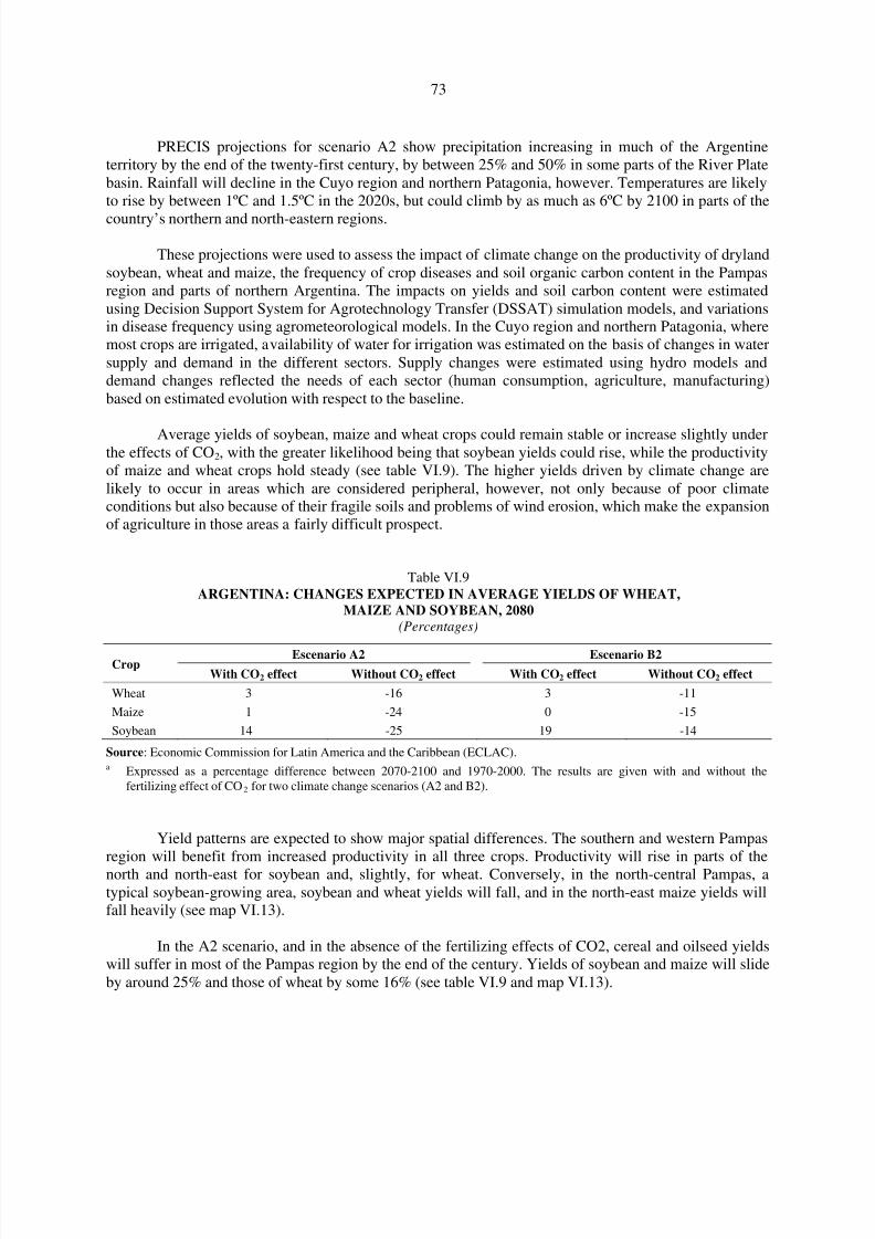
8/8/2019 CEPAL Climate Change 2010
http://slidepdf.com/reader/full/cepal-climate-change-2010 73/107
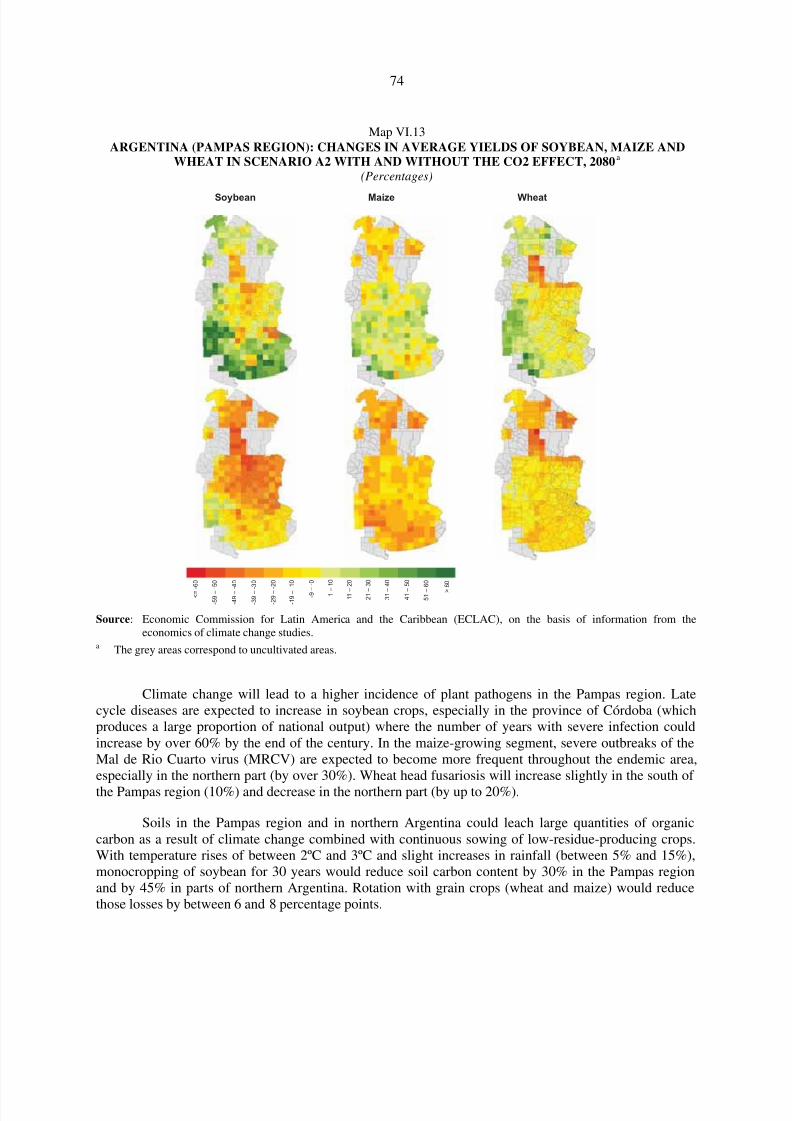
8/8/2019 CEPAL Climate Change 2010
http://slidepdf.com/reader/full/cepal-climate-change-2010 74/107
74
Map VI.13ARGENTINA (PAMPAS REGION): CHANGES IN AVERAGE YIELDS OF SOYBEAN, MAIZE AND
WHEAT IN SCENARIO A2 WITH AND WITHOUT THE CO2 EFFECT, 2080a
(Percentages)
Source: Economic Commission for Latin America and the Caribbean (ECLAC), on the basis of information from theeconomics of climate change studies.
a The grey areas correspond to uncultivated areas.
Climate change will lead to a higher incidence of plant pathogens in the Pampas region. Latecycle diseases are expected to increase in soybean crops, especially in the province of Córdoba (whichproduces a large proportion of national output) where the number of years with severe infection couldincrease by over 60% by the end of the century. In the maize-growing segment, severe outbreaks of theMal de Rio Cuarto virus (MRCV) are expected to become more frequent throughout the endemic area,especially in the northern part (by over 30%). Wheat head fusariosis will increase slightly in the south of the Pampas region (10%) and decrease in the northern part (by up to 20%).
Soils in the Pampas region and in northern Argentina could leach large quantities of organiccarbon as a result of climate change combined with continuous sowing of low-residue-producing crops.With temperature rises of between 2ºC and 3ºC and slight increases in rainfall (between 5% and 15%),monocropping of soybean for 30 years would reduce soil carbon content by 30% in the Pampas regionand by 45% in parts of northern Argentina. Rotation with grain crops (wheat and maize) would reducethose losses by between 6 and 8 percentage points.
< = - 6 0
- 5 9 – - 5 0
- 4 9 – - 4 0
- 3 9 – - 3 0
- 2 9 – - 2 0
- 1 9 – - 1 0
- 9 –
- 0
1 –
1 0
1 1 –
2 0
2 1 –
3 0
3 1 –
4 0
4 1 –
5 0
5 1 –
6 0
>
6 0
Soybean Maize Wheat
8/8/2019 CEPAL Climate Change 2010
http://slidepdf.com/reader/full/cepal-climate-change-2010 75/107
75
Fruit- and vegetable-growing will suffer in northern Patagonia. The projected drop in rainfall willreduce average flows in the River Neuquén by between 24% in scenario B2 and 35% in scenario A2,which will affect horticultural activity in the region, including the growing of pip fruits (apples andpears), vines and, to a lesser extent, stone fruits.
As of 2030, the availability of water for irrigation in the northern part of the Mendoza basin is likelyto run into difficulties. In 2000, this basin, part of the Cuyo region, accounted for 75% of Mendoza’s vineplantations and 55% of its garlic plantations. Surface water here is taken up entirely by the various users,and when it becomes scarce 70% of the cultivated area relies on underground water resources. Even in themost benevolent scenario, the projected rise in demand merely from the population growth estimated at2030 will compromise the availability of subterranean water for irrigation, pushing up irrigation costs tolevels (4,500 Argentine pesos per hectare per year) that will force many producers out of farming. Inaddition, water quality will be reduced by the worsening of existing salinization processes.
2. Chile
Since the 1970s, precipitation has declined in the central and southern parts of Chile and temperatureshave climbed in the central valley, especially in the mountainous areas. Conversely, temperatures havefallen in the coastal areas.
PRECIS projections indicate widespread temperature rises which, in the short term, will besharpest in the Altiplano. By the end of the twenty-first century, temperatures will have risen by between3ºC and 4ºC in scenario A2 and by between 2ºC and 3ºC in scenario B2 throughout Chile, including in thefar south. The further away from the ocean (by distance from the coast or altitude), the sharper thetemperature rises. In both the A2 and B2 scenarios, precipitation will drop by between 10% and 20% inthe Norte Chico region in the short term (2020-2040). In the medium term (2040-2070), precipitation willfall in the regions of Antofagasta and Los Lagos and increase in Magallanes. By 2100, precipitation
between Antofagasta and the Los Lagos region will have dwindled by up to 40% in scenario A2, butincreased in the far south and the Altiplano.
On the basis of these projections, impacts on the productivity of annual crops, fruit species(including vines), pastures and forestry plantations were estimated using the SIMPROC simulationmodel, which is capable of regulating irrigation according to existing constraints on availability of waterfor irrigated crops.
Water will be one of the main constraints on agriculture in the central and central northern partsof Chile. In basins situated between 30º and 42º latitude south (north of the River Maipo) the availabilityof irrigation water will decrease during critical periods (late spring and summer), as water flows declineand their timing shifts and as ice masses built up in glaciers gradually disappear. In the period 2010-2040
water availability will decrease by 15% in the Aconcagua basin (scenario A2) and towards the end of thecentury (2070-2100), the decline will vary between 30% in the Maipo basin (scenario B2) and 65% in theAconcagua basin (scenario A2). To the south of the River Maipo, although precipitation will decline andtemperatures will rise, there is enough spare water availability to suppose that agriculture and forestry willbe spared from major impacts. Meanwhile, in the far north of Chile (the Altiplano and landlocked basins)water availability is uncertain, but will probably decline in the near future before expanding towards theend of the century.

8/8/2019 CEPAL Climate Change 2010
http://slidepdf.com/reader/full/cepal-climate-change-2010 76/107
76
Atmospheric warming, water shortages and increased evapotranspiration will reduce productivityin northern and central Chile. Conversely, rising temperatures, more moderate frosts and more abundantwater will benefit the south. Winter crops (wheat, oats and barley), fruit, vines and radiata pineplantations will become less productive in the northern and central zones, except for certain areas of the
central valley where cereal productivity could edge up. All species will benefit in the south (see mapVI.14). Deciduous fruit trees —pomes, raspberries, blueberries and cherries— will fare worst: they willno longer have the many hours of cool they need and they are particularly sensitive to high temperatures.Conditions will be especially inclement for these fruits in the central valley from the 2050s onward. Stonefruits and vines will sustain smaller impacts, being less sensitive to the variables mentioned.
Map VI.14CHILE: RELATIVE CHANGES IN PRODUCTIVITY OF DRYLAND WHEAT, VINES, NATURAL
PASTURE AND RADIATA PINE IN THE A2 CLIMATE CHANGE SCENARIO, 2040-2070(Percentages)
Source: Centro de Agricultura y Medio Ambiente (AGRIMED), Análisis de vulnerabilidad del sector silvoagropecuario, recursos
hídricos y edáficos de Chile frente a escenarios de cambio climático. Segunda comunicación nacional de Chile, Santiago,Chile, 2008.
Forestry and agricultural activities are expected to shift towards the south (Araucanía, Los Ríosand Los Lagos), where the climate will become more apt for them (see figure VI.2). An econometricmodel developed to estimate potential land use change in response to climate-driven shifts in landprofitability found that the cultivated area would remain constant over time, but that the allocation of activities would change.
Wheat Vines Pasture Radiata pine

8/8/2019 CEPAL Climate Change 2010
http://slidepdf.com/reader/full/cepal-climate-change-2010 77/107
77
Figure VI.2CHILE: CULTIVATED AREA
(Thousands of hectares)
A. Area currently devoted to crops, B. Changes expected in area devoted
fruit trees, forestry species to each activity in A2 climateand pasture (10 regions a) change scenario, 2070-2100
Source: Economic Commission for Latin America and the Caribbean (ECLAC).a The regions appear in order of north to south.
Higher temperatures could enable the cultivation of subtropical species almost throughout Chile.Milder winters could make it possible to grow crops which are not viable today because of frost andtemperatures too low for their needs.
3. Ecuador
The changes observed in Ecuador’s climate in the past few decades consist of average temperature risesof between 0.5oC and 1.6oC, depending on the area, and irregular rainfall patterns with declines inseaward regions. Estimates carried out using the PRECIS model for scenario A2 suggests highertemperatures, especially in the sierra and the Amazon region. Temperature rises would be smaller in theB2 scenario. Precipitation will tend to increase on the coast and in the Amazon region and decline in thesierra. The study used statistical functions to quantify the impact on productivity of changes in climatevariables. The dependent variable adopted for the equations was average provincial yields during 1985-2008, and the independent variables were different combinations of temperature and precipitation andclimatic anomalies, according to the effects they would theoretically have at the most sensitive stage of each crop’s development.
Coffee, bananas, cacao and sugarcane will be the crops worst affected by climate change inEcuador. In both scenarios these crops will lose productivity, slightly in the short term (2020) and moreheavily towards the end of the century (2080), with losses of almost 20% in coffee and cacao and 40% inbananas and sugarcane. Climate change will threaten food security, given that productivity will declinefor beans and, particularly, for soft maize, which are both sown mainly by small farmers in the sierra. Thesharpest reductions (as much as 40%) occur in soft maize towards the end of the century in climatechange scenario A2. Conversely, rice and durum maize will gain from climate change and theirproductivity could hold steady or even climb by 25% or 30% by the end of the century.
0
500
1 000
1 500
2 000
2 500
3 000
3 500
-100
-75
-50
-25
0
25
50
75
100
A t a
c a m a
C o q
u i m b o
V a l p a r a í s o
R
e g i ó n
M e t r o p o
l i t a n a
O ' H
i g g i n s
M a u l e
B
í o B í o
A r a u
c a n í a
L o s R í o s
L o s
L a g o s
A t a c a m a
C o q
u i m b o
V a l p
a r a í s o
R
e g i ó n
M e t r o p o
l i t a n a
O ' H
i g g i n s
M a u l e
B
í o B í o
A r a u c a n í a
L o s R í o s
L o s L a g o s
Crops Fruit trees Forestry Pasture
8/8/2019 CEPAL Climate Change 2010
http://slidepdf.com/reader/full/cepal-climate-change-2010 78/107
78
Land availability is a key factor for production. For all the crops assessed, it was the factor mostclosely tied to productivity and was more important than availability of labour or irrigation infrastructure.Subsistence farmers working at higher altitudes, where the current temperature is below the optimumrequired for several species, could benefit from temperature rises.
4. Paraguay
Paraguay is South America’s most rural country. Its agricultural sector accounts for between 17% and20% of GDP and much of its population depends directly or indirectly on the activity. Soybean-growingis one of the largest segments within agriculture. In 2007-2008 the soybean crop contributed 17% of Paraguay’s GDP and over 45% of export revenues. The bulk of soybean (98%) is grown as a dryland cropand it is highly sensitive to yearly variations in climate, especially in rainfall.
The climate changes observed in the past few decades consist of higher temperatures and increasingprecipitation, especially in the east of the country. Climate projections derived from PRECIS modelling
indicate end-of-century temperature rises of about 4.3ºC in scenario A2 and 3.4ºC in scenario B2, and slightincreases in precipitation —larger in the A2 scenario— especially during the rainiest period.
On the basis of these climate scenarios, the impacts on the agricultural sector were analysed forfamily farms (70% of them producing sugarcane, cotton, sesame and manioc as cash crops), corporateagriculture (which produces mainly soybean, wheat, maize and sunflowers), and beef farming.Departmental statistical relations were drawn between yield or productivity (1992-2008) and variations inclimate variables. For most crops, the analysis encompassed both seasons of the growth cycle. For annualcrops (manioc and sugarcane) annual average temperatures and precipitation were used.
Temperature rises and rainfall distribution changes will do damage to some areas that areimportant for the Paraguayan economy. Yields of soybean and wheat and the productivity of beef-raising,
two key activities in the country’s agricultural sector, will both fall. Beef livestock production will be theactivity hardest hit by climate change. By the end of the twenty-first century, beef production will havefallen by around 27% in the A2 scenario or 22% in the B2 scenario (see table VI.10). In terms of 2008GDP, the decline in beef production will represent losses equivalent to 1.8% by mid-century and 6.6% atthe end of the century.
Soybean-growing will be the worst affected segment of agriculture. In scenario A2 soybeanyields will slide by 10% by mid-century and by 15% by the end of the century (see table VI.10) or, interms of 2008 GDP, by 1.9% and 3% by 2050 and 2080, respectively. Wheat productivity will alsodeteriorate, with yields expected to fall by 9% by mid-century and 13% by the end of the century inscenario A2, or 0.3% and 0.5% of 2008 GDP, respectively. Cotton-growing will suffer slightly too, withyield reductions of up to 6% by 2050.
The productivity of some crops which are important in family farming could hold steady or rise.This is the case for sesame, beans, manioc and sugarcane (see table VI.10), which are the main cash cropsfor small family farms. These outcomes are highly uncertain, however, given the low explanatory powerof climate variables in the equations performed. Family farming will be highly vulnerable to non-climatestress factors, however, which will intensify throughout the twenty-first century, such as soil degradationresulting from overexploitation and declining labour as producers age and younger population groupsmigrate to the cities.
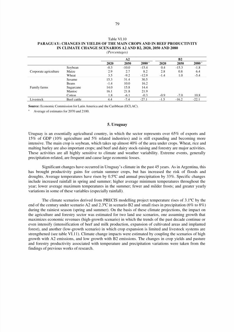
8/8/2019 CEPAL Climate Change 2010
http://slidepdf.com/reader/full/cepal-climate-change-2010 79/107
79
Table VI.10PARAGUAY: CHANGES IN YIELDS OF THE MAIN CROPS AND IN BEEF PRODUCTIVITY
IN CLIMATE CHANGE SCENARIOS A2 AND B2, 2020, 2050 AND 2080(Percentages)
A2 B22020 2050 2080 a
2020 2050 2080 a
Corporate agricultureSoybean -0.3 -10.0 -15.4 0.4 -15.3 -1.8Maize 2.9 2.7 8.2 2.8 0.8 6.4Wheat 3.5 -9.2 -12.9 -1.4 1.0 -5.4
Family farms
Sesame 15.3 31.4 30.5Beans -1.4 10.0 16.2Sugarcane 14.0 15.8 14.4Manioc 16.1 21.8 21.9Cotton 1.8 -6.1 -0.3 -0.9 -7.0 10.8
Livestock Beef cattle 4.4 -7.4 -27.1 -1.5 -16.2 -22.1
Source: Economic Commission for Latin America and the Caribbean (ECLAC).a Average of estimates for 2070 and 2100.
5. Uruguay
Uruguay is an essentially agricultural country, in which the sector represents over 65% of exports and15% of GDP (10% agriculture and 5% related industries) and is still expanding and becoming moreintensive. The main crop is soybean, which takes up almost 40% of the area under crops. Wheat, rice andmalting barley are also important crops; and beef and dairy stock-raising and forestry are major activities.These activities are all highly sensitive to climate and weather variability. Extreme events, generallyprecipitation-related, are frequent and cause large economic losses.
Significant changes have occurred in Uruguay’s climate in the past 45 years. As in Argentina, thishas brought productivity gains for certain summer crops, but has increased the risk of floods anddroughts. Average temperatures have risen by 0.5ºC and annual precipitation by 33%. Specific changesinclude increased rainfall in spring and summer; higher average minimum temperatures throughout theyear; lower average maximum temperatures in the summer; fewer and milder frosts; and greater yearlyvariations in some of these variables (especially rainfall).
The climate scenarios derived from PRECIS modelling project temperature rises of 3.1ºC by theend of the century under scenario A2 and 2.3ºC in scenario B2 and small rises in precipitation (6% to 8%)during the rainiest season (spring and summer). On the basis of these climate projections, the impact onthe agriculture and forestry sector was estimated for two land use scenarios, one assuming growth thatmaximizes economic revenues (high-growth scenario) in which the trends of the past decade continue oreven intensify (intensification of beef and milk production, expansion of cultivated areas and implantedforest), and another (low-growth scenario) in which crop expansion is limited and livestock systems are
strengthened (see table VI.11). Climate change impacts were estimated by coupling the scenarios of highgrowth with A2 emissions, and low growth with B2 emissions. The changes in crop yields and pastureand forestry productivity associated with temperature and precipitation variations were taken from thefindings of previous works of research.
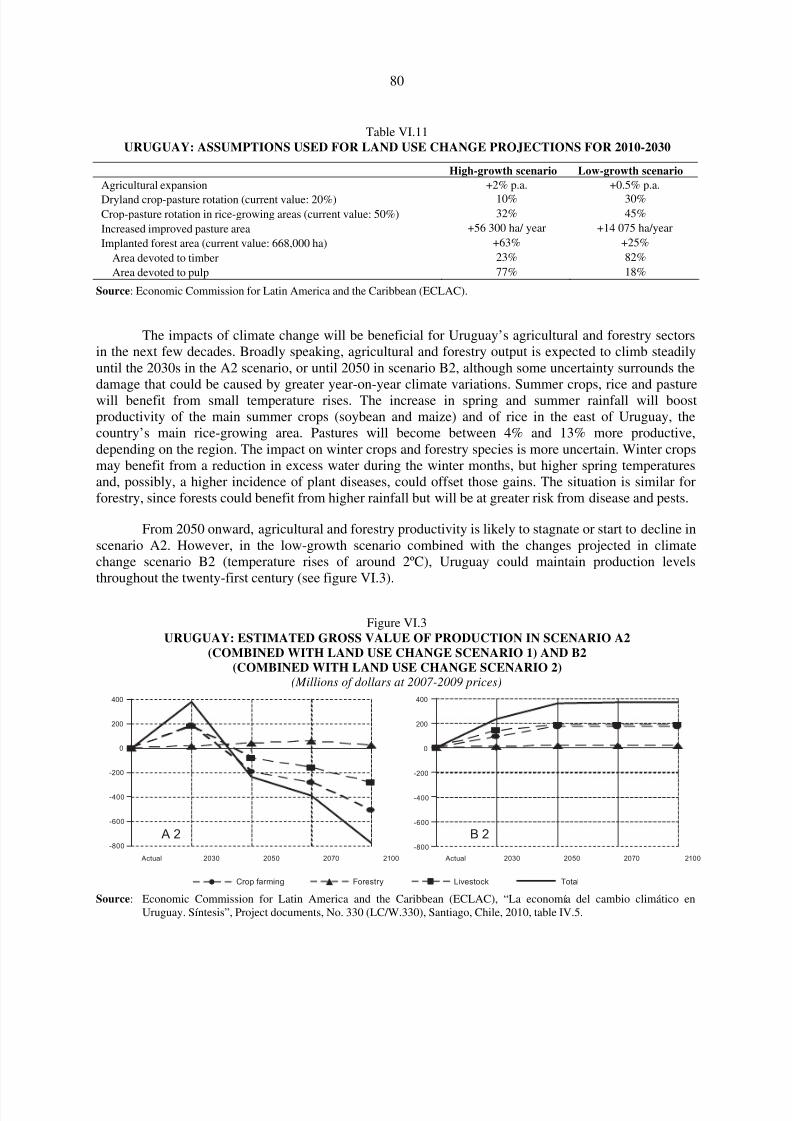
8/8/2019 CEPAL Climate Change 2010
http://slidepdf.com/reader/full/cepal-climate-change-2010 80/107
80
Table VI.11URUGUAY: ASSUMPTIONS USED FOR LAND USE CHANGE PROJECTIONS FOR 2010-2030
High-growth scenario Low-growth scenario
Agricultural expansion +2% p.a. +0.5% p.a.
Dryland crop-pasture rotation (current value: 20%) 10% 30%Crop-pasture rotation in rice-growing areas (current value: 50%) 32% 45%
Increased improved pasture area +56 300 ha/ year +14 075 ha/year
Implanted forest area (current value: 668,000 ha) +63% +25%
Area devoted to timber 23% 82%
Area devoted to pulp 77% 18%
Source: Economic Commission for Latin America and the Caribbean (ECLAC).
The impacts of climate change will be beneficial for Uruguay’s agricultural and forestry sectorsin the next few decades. Broadly speaking, agricultural and forestry output is expected to climb steadilyuntil the 2030s in the A2 scenario, or until 2050 in scenario B2, although some uncertainty surrounds thedamage that could be caused by greater year-on-year climate variations. Summer crops, rice and pasturewill benefit from small temperature rises. The increase in spring and summer rainfall will boostproductivity of the main summer crops (soybean and maize) and of rice in the east of Uruguay, thecountry’s main rice-growing area. Pastures will become between 4% and 13% more productive,depending on the region. The impact on winter crops and forestry species is more uncertain. Winter cropsmay benefit from a reduction in excess water during the winter months, but higher spring temperaturesand, possibly, a higher incidence of plant diseases, could offset those gains. The situation is similar forforestry, since forests could benefit from higher rainfall but will be at greater risk from disease and pests.
From 2050 onward, agricultural and forestry productivity is likely to stagnate or start to decline inscenario A2. However, in the low-growth scenario combined with the changes projected in climatechange scenario B2 (temperature rises of around 2ºC), Uruguay could maintain production levelsthroughout the twenty-first century (see figure VI.3).
Figure VI.3URUGUAY: ESTIMATED GROSS VALUE OF PRODUCTION IN SCENARIO A2
(COMBINED WITH LAND USE CHANGE SCENARIO 1) AND B2(COMBINED WITH LAND USE CHANGE SCENARIO 2)
(Millions of dollars at 2007-2009 prices)
Source: Economic Commission for Latin America and the Caribbean (ECLAC), “La economía del cambio climático enUruguay. Síntesis”, Project documents, No. 330 (LC/W.330), Santiago, Chile, 2010, table IV.5.
Total
0 0
400
200
-200
-400
-600
-800
Actual 2030 2050 2070 2100
400
200
-200
-400
-600
-800
Actual 2030 2050 2070 2100
A 2 B 2
Crop farming Forestry Livestock

8/8/2019 CEPAL Climate Change 2010
http://slidepdf.com/reader/full/cepal-climate-change-2010 81/107
81
6. Central America
Agriculture is one of the economic engines of Central America, representing some 11% of total GDP, or18% if agro-industry is included.5 It is also the main supplier of foodstuffs and inputs for industry, and
contributes 35% of total exports. Agriculture and the rural milieu absorb a large proportion of the laboursupply and represent a major source of income for rural households. However, production is not fast-growing and yields have stagnated, which undermines the sector’s competitiveness and growth potential.This low productivity is attributable to poor capitalization and damage caused by climate phenomena,among other factors.
Extreme events have become much more frequent in the past four decades, and especially in thelast 10 years. In particular, powerful hurricanes have wrought devastation on the agricultural sector.Between 1972 and 2007 extreme events caused losses of US$ 11 billion (5.7% of Central America’s GDPat 2007 prices), of which US$ 3.7 billion was in the agricultural sector. Around 60% of those lossesoccurred during Hurricane Mitch in 1998, in which Honduras was particularly badly hit.
Analysis of climate change impacts on agriculture in Central America was based on theproduction function and examined the effects of temperature and precipitation variables on agriculturaloutput, crop and cereal production, and livestock raising. A second strand of the analysis aimed toidentify the impacts of climate variables on average yields of staple crops of maize, beans and rice.
Past temperature patterns show a temperature rise of almost 1oC since the 1970s, except in Belize(about 0.7oC) and Panama (0.5oC). In 1980-2006 some countries recorded a slight fall in precipitationlevels, especially El Salvador and Guatemala, whose rainfall has decreased by 3.6% and 2.7%,respectively. Precipitation has also declined in Honduras, by 1.2%. Average precipitation levels havebeen fairly stable in Nicaragua and Costa Rica (down 0.4% and up 0.6%, respectively), but are rising inBelize (2.7%) and Panama (3.4%).
The climate projections used in the study are derived from the average of three widely usedmodels for scenario A2 and for scenario B2. The changes projected for the rest of the century includewidespread reductions in precipitation and higher temperatures. Rainfall declines more heavily and ismore variable, and temperatures rise further, in scenario A2 than in B2. On the basis of thesescenarios, temperature and precipitation variations were incorporated into production functions,assuming the absence of technological change and no adaptation by farmers to the effects of climatechange. Figure VI.4 shows the modelling of agricultural production indices using the averages of models for scenarios A2 and B2.
In Central America the temperatures today are close to or slightly higher than optimumtemperatures for agriculture. Accordingly, the warming expected for the rest of the twenty-first century,combined with more variable rainfall, is expected to reduce the productivity of the agricultural sector. The
findings indicate adverse effects in the final decades of the century in all indices in the A2 scenario, andin the livestock index in scenario B2. For example, by 2100 the agricultural production index drops byapproximately 9% in the A2 scenario, and by 3% in the B2. The crop farming index declines by about10% in scenario A2 and 3% in B2, whereas the livestock index falls by 13% in A2 and 5% in B2.
5 These data do not include Belize.

8/8/2019 CEPAL Climate Change 2010
http://slidepdf.com/reader/full/cepal-climate-change-2010 82/107
82
Figure VI.4
CENTRAL AMERICA: CHANGE IN AGRICULTURAL INDEX IN CLIMATECHANGE SCENARIOS B2 AND A2, 2006-2100 a
Source: Economic Commision for Latin America and the Caribbean (ECLAC).a Calculated using a Hodrick-Prescott filter.
The impacts on the production of maize, beans and rice were also analysed. For maize, the optimumtemperature in the region is around 26.5°C, which enables production of almost 2 tons per hectare. Giventhe current temperatures, the maize crop could tolerate increases of between 1°C and 2°C, which would notsignificantly affect yields. But if the average temperature rises by more than 2°C, losses in maizeproductivity will be inevitable. The findings for precipitation show that the current average level is farbelow the optimum. In scenario A2 the yield would hold steady around the historical average of 2 tons perhectare in the short term, but would then decline to 1.4 tons per hectare around 2100 (see figure VI.5). Inscenario B2 maize production would not sustain any great impact until the end of the century. The analysesfor each country identify grave threats to the maize yield in scenario A2 by the end of the century. Yields inEl Salvador, Guatemala and Panama could fall very far unless adaptation measures are taken.
For bean production, the regional average temperature has already exceeded the optimum yieldlevel by about 2.5°C and the current precipitation level falls slightly short of that needed for maximumyield. Larger temperature rises and reductions or greater variability in rainfall are likely to affect beanproduction quite seriously. In both scenarios, A2 and B2, the bean yield falls substantially, from over0.7 tons per hectare to less than 0.1 tons per hectare in A2 and to 0.5 tons per hectare in B2 by 2100. Theanalyses by country identify grave threats to bean yields in scenario A2 by the end of the century.According to some of the specifications used, yields could fall drastically in Guatemala and El Salvador(without considering adaptation measures). In Belize bean yields fall to 0.2 tons per hectare in A2 by theend of the century. Given that many bean growers are small farmers, have scant resources and low yields,the impact of even a 1°C-2°C temperature rise —still short of the upper limit of 4°C-5°C— would havemajor repercussions throughout the region, endangering the food security of large segments of thepopulation (see figure VI.6).
88
92
96
100
104
108
2020 2040 2060 2080 2100
Years
Scenario B2 Scenario A2
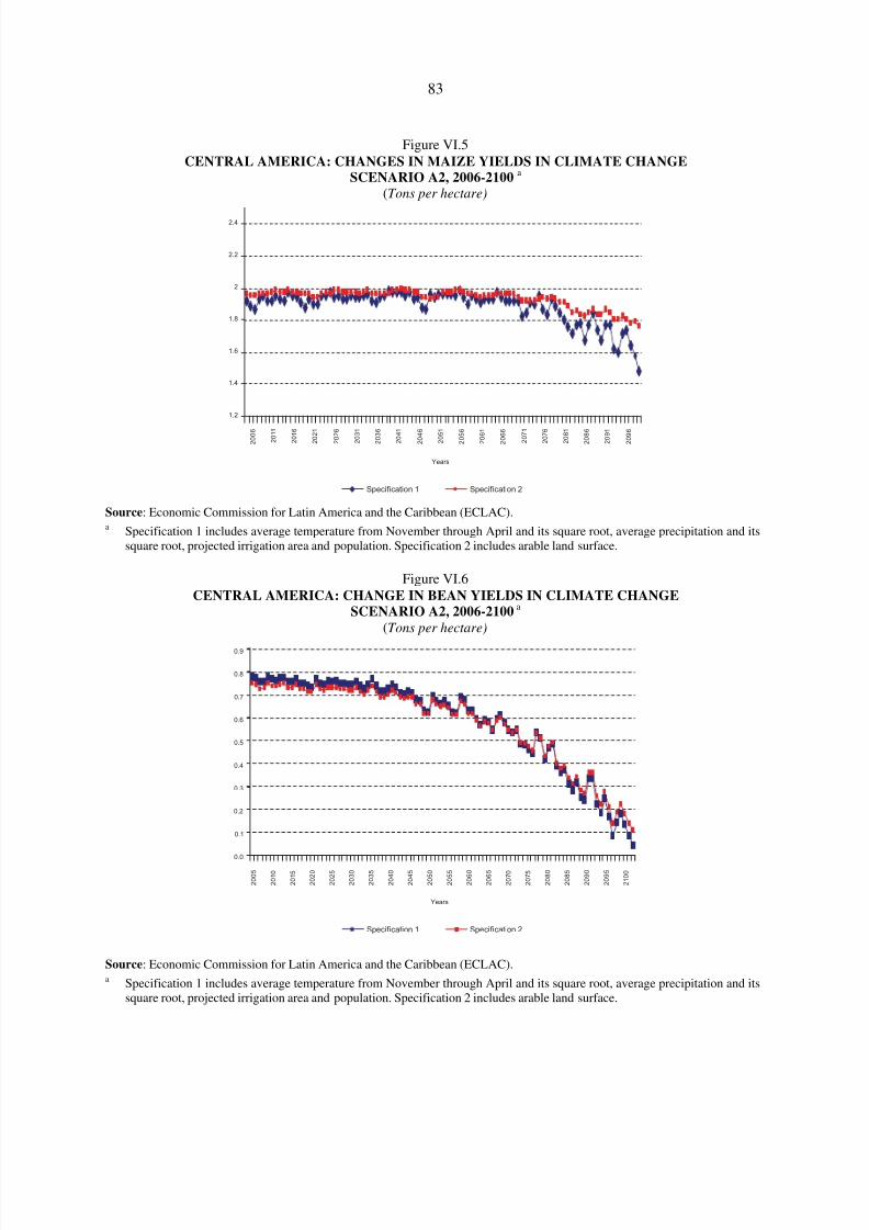
8/8/2019 CEPAL Climate Change 2010
http://slidepdf.com/reader/full/cepal-climate-change-2010 83/107
83
Figure VI.5
CENTRAL AMERICA: CHANGES IN MAIZE YIELDS IN CLIMATE CHANGESCENARIO A2, 2006-2100 a
(Tons per hectare)
Source: Economic Commission for Latin America and the Caribbean (ECLAC).a Specification 1 includes average temperature from November through April and its square root, average precipitation and its
square root, projected irrigation area and population. Specification 2 includes arable land surface.
Figure VI.6
CENTRAL AMERICA: CHANGE IN BEAN YIELDS IN CLIMATE CHANGESCENARIO A2, 2006-2100
a (Tons per hectare)
Source: Economic Commission for Latin America and the Caribbean (ECLAC).a Specification 1 includes average temperature from November through April and its square root, average precipitation and its
square root, projected irrigation area and population. Specification 2 includes arable land surface.
Years
Specification 1 Specification 2
2 0 0 6
2 0 1 1
2 0 1 6
2 0 2 1
2 0 2 6
2 0 3 1
2 0 3 6
2 0 4 1
2 0 4 6
2 0 5 1
2 0 5 6
2 0 6 1
2 0 6 6
2 0 7 1
2 0 7 6
2 0 8 1
2 0 8 6
2 0 9 1
2 0 9 6
2.4
2.2
2
1.8
1.6
1.4
1.2
Years
Specification 1 Specification 2
0.9
0.8
0.7
0.6
0.5
0.4
0.3
0.2
0.1
0.0
2 0 0 5
2 0 1 0
2 0 1 5
2 0 2 0
2 0 2 5
2 0 3 0
2 0 3 5
2 0 4 0
2 0 4 5
2 0 5 0
2 0 5 5
2 0 6 0
2 0 6 5
2 0 7 0
2 0 7 5
2 0 8 0
2 0 8 5
2 0 9 0
2 0 9 5
2 1 0 0

8/8/2019 CEPAL Climate Change 2010
http://slidepdf.com/reader/full/cepal-climate-change-2010 84/107
84
Rice-growing is at a delicate juncture. The current average temperature is compatible withoptimum productivity, which will remain relatively stable with a temperature rise of up to 1.5°C, though alarger rise would bring adverse effects. The region’s current average precipitation is compatible withoptimum yield, but yields will start to fall when the decline in rainfall reaches 15%. In the 2100 scenarios,
production will tend to drop from the historical average of 3.5 tons per hectare to between 1 and 2 tonsper hectare in A2. In Panama, unless adaptation measures are taken, the rice yield could drop to criticallevels in the final decades of the century in scenario A2 (see figure VI.7).
Figure VI.7CENTRAL AMERICA: CHANGE IN RICE YIELDS IN CLIMATE CHANGE
SCENARIO A2, 2006-2100a
(Tons per hectare)
Source: Economic Commission for Latin America and the Caribbean (ECLAC).a Specification 1 includes average temperature from November through April and its square root, average precipitation and its
square root, projected irrigation area and population. Specification 2 includes arable land surface.
Because of the way that agricultural production is tied in with other sectors of the economy—such as the production of processed foods, the household economy of small farmers andagricultural workers, the manufacturing sector and the increased importation of agricultural products—the impact of climate change will push up costs considerably for the subregion as a whole. Althoughthese costs will remain relatively low for the first half of the twenty-first century, they will rise rapidly
after 2050, particularly in scenario A2.
Beyond this initial estimate of impacts on yields and their economic implications, the fact is thatmaize, beans and rice are dietary staples for much of the Central American population, since many small,low-income farmers consume much of their crop themselves. Accordingly, the effect of climate changeon agricultural activities will have significant repercussions for food security, since it will reduce theproduction of food and rural producers’ direct access to it, and lead to scarcity and higher prices,depending on the possibility of importing food to compensate. The implications are therefore serious forboth food security and poverty.
Years
Specification 1 Specification 2
4.0
3.5
3.0
2.5
2.0
1.5
1.0
0.5
2 0 0 6
2 0 1 1
2 0 1 6
2 0 2 1
2 0 2 6
2 0 3 1
2 0 3 6
2 0 4 1
2 0 4 6
2 0 5 1
2 0 5 6
2 0 6 1
2 0 6 6
2 0 7 1
2 0 7 6
2 0 8 1
2 0 8 6
2 0 9 1
2 0 9 6
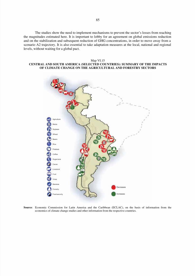
8/8/2019 CEPAL Climate Change 2010
http://slidepdf.com/reader/full/cepal-climate-change-2010 85/107
85
The studies show the need to implement mechanisms to prevent the sector’s losses from reachingthe magnitudes estimated here. It is important to lobby for an agreement on global emissions reductionand on the stabilization and subsequent reduction of GHG concentrations, in order to move away from ascenario A2 trajectory. It is also essential to take adaptation measures at the local, national and regional
levels, without waiting for a global pact.
Map VI.15CENTRAL AND SOUTH AMERICA (SELECTED COUNTRIES): SUMMARY OF THE IMPACTS
OF CLIMATE CHANGE ON THE AGRICULTURAL AND FORESTRY SECTORS
Source: Economic Commission for Latin America and the Caribbean (ECLAC), on the basis of information from theeconomics of climate change studies and other information from the respective countries.
Agriculture
Maize
Soybean
Wheat
Beans
Rice
Potatoes
Coffee
Sugarcane
Cacao
Livestock
Fruit
Vines
Bananas
Forestry
Food security
Decreases
Increases

8/8/2019 CEPAL Climate Change 2010
http://slidepdf.com/reader/full/cepal-climate-change-2010 86/107
86
Box VI.3LATIN AMERICA AND THE CARIBBEAN: LAND DEGRADATION AND CLIMATE CHANGE
Land degradation or loss of soil biological and economic productivity is occurring in much of the Latin Americanand Caribbean region. It happens slowly and its effects usually become apparent over the long term, but the
deterioration is irreversible or very difficult to redress. Added to this phenomenon are large migratory movements of both people and production activities, often because of erosion resulting from deforestation, the overexploitation of land for agriculture and contamination with chemical products. The destruction of plant cover, especiallydeforestation for timber and agricultural purposes, generates GHG emissions. In Latin America and the Caribbean,land use change is one of the main sources of GHG emissions together with the energy sector.
The higher temperatures and changes in precipitation patterns associated with climate change affectproductivity and the process of land degradation, for example, by increasing aridity and the number of dry monthsper year (thus interfering with the precipitation–evapotranspiration cycle), which has the effect of concentratingprecipitation and making it more aggressive. Some of the worst affected areas are on the agricultural frontier in veryfragile ecosystems such as the edges of the Amazon forest in Colombia, Ecuador and Peru, where human activitiessuch as deforestation, agriculture, livestock-raising and informal gold mining are causing severe degradation.
Land degradation can compromise extensive areas very rapidly. For example, according to data from theGlobal Land Degradation Assessment and Improvement (GLADA) project, between 1982 and 2002 additional
degraded areas totalled 16.4% of the territory of Paraguay, 15.3% of Peru and 14.2% of Ecuador. If this trendcontinues until the end of the century, it is estimated that 66.3% of the territory of Paraguay, 62% of Peru and 57.2%of Ecuador will become degraded.
LATIN AMERICA (SELECTED COUNTRIES): PROJECTIONS OF DEGRADED AREAS, 2050 AND 2100(Percentages of each country’s territory)
Country 2050 2100
Chile 20.8 41.2Ecuador 28.9 57.2Bolivia (Plurinational State of) 11.2 22.2Paraguay 33.5 66.3Peru 31.3 62.0
Climate change is adding to the impact of the degradation produced by human activity. Degradationassessments in Ecuador show that the main agents of land degradation will continue to be anthropic up to 2050, but
the effects of climate change will gain increasing significance during the second half of the twenty-first century andparticularly towards 2100.
In the Chaco region of Paraguay, now a dry area, rainfall will increase and become concentrated in a fewmonths of the year, which will deepen vulnerability to degradation. Aridity will decrease in the north of Peru due torising precipitation but, like in Paraguay, its marked seasonality and concentration in few months will increasevulnerability to degradation. A similar situation will occur in the eastern region of the Plurinational State of Bolivia.In Chile, conversely, arid and semi-arid zones will expand, owing to higher temperatures and declining rainfall,leading to a southward shift of central and southern-central agricultural activities. This will create a need for newinvestments in infrastructure for irrigation and water storage and distribution, to enable production in new areas.
In the case of Central America, estimates based on the current situation and projections to 2100 suggest thatstaple crop yields will fall heavily in all the countries except El Salvador, as a result of advancing degradationprocesses. In Guatemala, it is estimated that the gross value of production will fall by 23% in scenario B2 and by 25%in scenario A2. In terms of the magnitude of losses, Guatemala is followed by Belize, Costa Rica and Honduras.
The worsening of land degradation in several Central American countries is particularly worrisome. Datafrom the GLADA project indicate that Guatemala suffered the fastest land degradation in the region between 1982and 2002 and the proportion of degraded land in the country is now 58.9%. GLADA data also show serious landdegradation in Costa Rica and Honduras, with degraded land proportions of 29.5% and 38.4%, respectively. Thefindings for El Salvador, however, suggest an improvement in land productivity, in other words, a relative reversalof degradation status. This may be attributable to that fact that severe anthropic degradation in the recent past isreflected in the baseline and has been reversed in the past two decades, because land exploitation has easedfollowing intensive migratory processes.
Source: Economic Commission for Latin America and the Caribbean (ECLAC), on the basis of data from the Global LandDegradation Assessment and Improvement (GLADA) project of the Global Environment Facility (GEF).
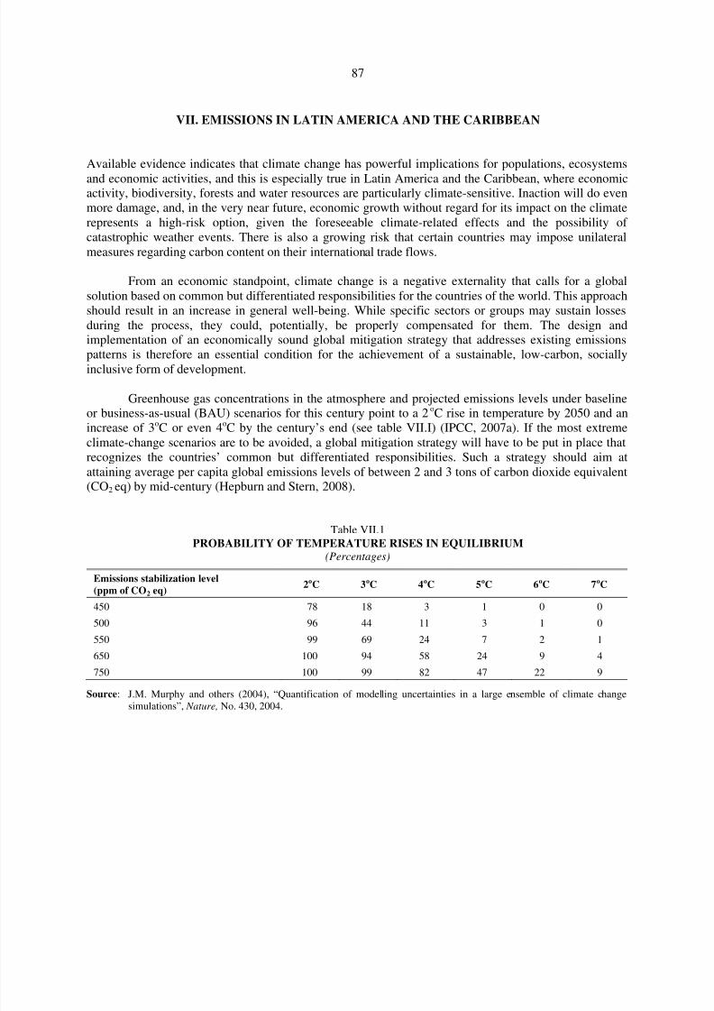
8/8/2019 CEPAL Climate Change 2010
http://slidepdf.com/reader/full/cepal-climate-change-2010 87/107
87
VII. EMISSIONS IN LATIN AMERICA AND THE CARIBBEAN
Available evidence indicates that climate change has powerful implications for populations, ecosystems
and economic activities, and this is especially true in Latin America and the Caribbean, where economicactivity, biodiversity, forests and water resources are particularly climate-sensitive. Inaction will do evenmore damage, and, in the very near future, economic growth without regard for its impact on the climaterepresents a high-risk option, given the foreseeable climate-related effects and the possibility of catastrophic weather events. There is also a growing risk that certain countries may impose unilateralmeasures regarding carbon content on their international trade flows.
From an economic standpoint, climate change is a negative externality that calls for a globalsolution based on common but differentiated responsibilities for the countries of the world. This approachshould result in an increase in general well-being. While specific sectors or groups may sustain lossesduring the process, they could, potentially, be properly compensated for them. The design andimplementation of an economically sound global mitigation strategy that addresses existing emissions
patterns is therefore an essential condition for the achievement of a sustainable, low-carbon, sociallyinclusive form of development.
Greenhouse gas concentrations in the atmosphere and projected emissions levels under baselineor business-as-usual (BAU) scenarios for this century point to a 2oC rise in temperature by 2050 and anincrease of 3oC or even 4oC by the century’s end (see table VII.I) (IPCC, 2007a). If the most extremeclimate-change scenarios are to be avoided, a global mitigation strategy will have to be put in place thatrecognizes the countries’ common but differentiated responsibilities. Such a strategy should aim atattaining average per capita global emissions levels of between 2 and 3 tons of carbon dioxide equivalent(CO2 eq) by mid-century (Hepburn and Stern, 2008).
Table VII.1PROBABILITY OF TEMPERATURE RISES IN EQUILIBRIUM
(Percentages)
Emissions stabilization level(ppm of CO2 eq)
2oC 3oC 4oC 5oC 6oC 7oC
450 78 18 3 1 0 0
500 96 44 11 3 1 0
550 99 69 24 7 2 1
650 100 94 58 24 9 4
750 100 99 82 47 22 9
Source: J.M. Murphy and others (2004), “Quantification of modelling uncertainties in a large ensemble of climate change
simulations”, Nature, No. 430, 2004.

8/8/2019 CEPAL Climate Change 2010
http://slidepdf.com/reader/full/cepal-climate-change-2010 88/107
88
Total global greenhouse gas emissions amounted to 44,130 metric tons of carbon dioxideequivalent (MtCO2 eq) in 2005 and increased at an average annual rate of 1.24% between 1990 and 2005(see figure VII.1).1 The Latin American and Caribbean region accounts for 5,390 MtCO2 eq, or 12% of total emissions worldwide. The rate of increase in emissions for the region —at 1.19% between 1990 and
2005– is similar to the global average (see figure VII.2). The distribution of emissions in the LatinAmerican and Caribbean region is quite uneven, however, with emissions being heavily concentrated incertain countries (see figure VII.2). Trends are also differentiated by source, as emissions from energysources are on the rise while those associated with changes in land use (deforestation) have more or lessbeen brought under control.
Figure VII.1AGGREGATE GREENHOUSE GAS EMISSIONS
(Percentages)
1 Greenhouse gas emissions are expressed in carbon dioxide equivalent (carbon dioxide in terms of global
warming potential measured over 100 years as set out in the Second Assessment Report of the IntergovernmentalPanel on Climate Change) (IPCC, 1995). The greenhouse gases included in this measurement are: carbondioxide (CO2), methane (CH4), nitrous oxide (N2O) and those with high warming potential, such ashydrofluorocarbons (HFC), perfluorocarbons (PFC) and sulphur hexafluoride (SF6). In keeping with the countryreports submitted under the United Nations Framework Convention on Climate Change, the energy sector,industrial processing and agriculture are taken into account, as well as changes in land and forest use and wastelevels. The energy sector is subdivided into electricity and heating, transportation, manufacturing andconstruction, other types of fuel-burning activities and fugitive gas emissions. The data on emissions wereobtained from the World Resource Institute (WRI), “Climate Analysis Indicators Tool (CAIT) Version 7.0”,2010 [online] www.cait.wri.org.
China
United States
European Union (27 countries)
Brazil, Indonesia, Russian Federation
India, Japan, Canada
Mexico, Rep. of Korea, Australia
Iran (Islamic Rep. of),Ukraine, Nigeria
Venezuela (Bol. Rep. of),South Africa, Turkey
Rest of world (170 countries)
0
10
20
30
40
50
60
70
80
90
100
A. 2005
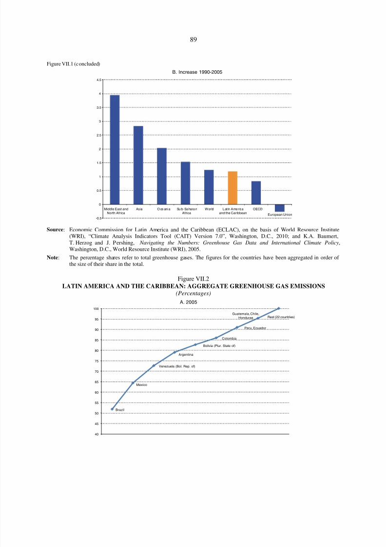
8/8/2019 CEPAL Climate Change 2010
http://slidepdf.com/reader/full/cepal-climate-change-2010 89/107
89
Figure VII.1 (concluded)
Source: Economic Commission for Latin America and the Caribbean (ECLAC), on the basis of World Resource Institute(WRI), “Climate Analysis Indicators Tool (CAIT) Version 7.0”, Washington, D.C., 2010; and K.A. Baumert,T. Herzog and J. Pershing, Navigating the Numbers: Greenhouse Gas Data and International Climate Policy,Washington, D.C., World Resource Institute (WRI), 2005.
Note: The percentage shares refer to total greenhouse gases. The figures for the countries have been aggregated in order of the size of their share in the total.
Figure VII.2
LATIN AMERICA AND THE CARIBBEAN: AGGREGATE GREENHOUSE GAS EMISSIONS(Percentages)
-0.5
0
0.5
1
1.5
2
2.5
3
3.5
4
4.5
Middle East andNorth Africa
As ia O ce ani a Su b- Sa hara nAfrica
Wor ld Lat in Amer icaand the Caribbean
OECD
European Union
B. Increase 1990-2005
Brazil
Mexico
Venezuela (Bol. Rep. of)
Argentina
Bolivia (Plur. State of)
Colombia
Peru, Ecuador
Guatemala, Chile,Honduras Rest (22 countries)
40
45
50
55
60
65
70
75
80
85
90
95
100
A. 2005
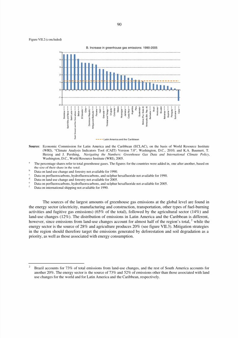
8/8/2019 CEPAL Climate Change 2010
http://slidepdf.com/reader/full/cepal-climate-change-2010 90/107
90
Figure VII.2 (concluded)
Source: Economic Commission for Latin America and the Caribbean (ECLAC), on the basis of World Resource Institute(WRI), “Climate Analysis Indicators Tool (CAIT) Version 7.0”, Washington, D.C., 2010; and K.A. Baumert, T.Herzog and J. Pershing, Navigating the Numbers: Greenhouse Gas Data and International Climate Policy,Washington, D.C., World Resource Institute (WRI), 2005.
a The percentage shares refer to total greenhouse gases. The figures for the countries were added in, one after another, based onthe size of their share in the total.
b Data on land use change and forestry not available for 1990.c Data on perfluorocarbons, hydrofluorocarbons, and sulphur hexafluoride not available for 1990.d Data on land use change and forestry not available for 2005.e Data on perfluorocarbons, hydrofluorocarbons, and sulphur hexafluoride not available for 2005.f Data on international shipping not available for 1990.
The sources of the largest amounts of greenhouse gas emissions at the global level are found inthe energy sector (electricity, manufacturing and construction, transportation, other types of fuel-burningactivities and fugitive gas emissions) (65% of the total), followed by the agricultural sector (14%) andland-use changes (12%). The distribution of emissions in Latin America and the Caribbean is different,however, since emissions from land-use changes account for almost half of the region’s total,2 while theenergy sector is the source of 28% and agriculture produces 20% (see figure VII.3). Mitigation strategiesin the region should therefore target the emissions generated by deforestation and soil degradation as a
priority, as well as those associated with energy consumption.
2 Brazil accounts for 73% of total emissions from land-use changes, and the rest of South America accounts foranother 20%. The energy sector is the source of 73% and 52% of emissions other than those associated with landuse changes for the world and for Latin America and the Caribbean, respectively.
-2
-1
0
1
2
3
4
5
D
o m i n i c a a , b , c , d , e
S a i n t K i t t s a n d N e v i s a , b , c , d , e
S a i n t L u c i a a , b , c , d , e
S a i n t V i n c e n t a n d t h e G r e
n a d i n e s a , b , c , d , e
B e l i z e a , b , c , d , e
E
l S a l v a d o r a , c , d
C h i l e a , c
D o m i n i c a n R e p u b l i c a , c , d
A n t i g u a a n d B a r b u d a a , b , c , d , e
P a n a m a a , c , d
H a i t i a , c , d
G r e n a d a a , b , c , d , e
T r i n i d a d a n d T o b a g o a , c , d
U r u g u a y a , c
C o l o m b i a a , c
M e x i c o
N i c a r a g u a a , c , d
J a m a i c a a , c , d
C
o s t a R i c a a , c , d
A r g e n t i n a
P e r u
G u a t e m a l a d
B o l i v i a ( P l u r . S t a t e o f )
V e n e z u e l a
( B o l . R e p . o f )
B
a r b a d o s a , b , c , d , e
B r a z i l
H o n d u r a s d
E c u a d o r
B
a h a m a s a , b , c , d , e
G u y a n a a , b , c , d , e
P a r a g u a y a , c , d
S
u r i n a m e a , b , c , d , e
C u b a a , c , d
Latin America and the Caribbean
B. Increase in greenhouse gas emissions: 1990-2005
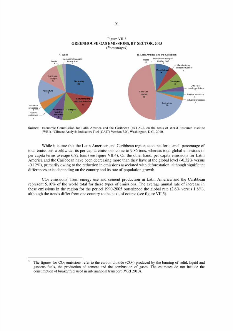
8/8/2019 CEPAL Climate Change 2010
http://slidepdf.com/reader/full/cepal-climate-change-2010 91/107
91
Figure VII.3GREENHOUSE GAS EMISSIONS, BY SECTOR, 2005
(Percentages)
Source: Economic Commission for Latin America and the Caribbean (ECLAC), on the basis of World Resource Institute(WRI), “Climate Analysis Indicators Tool (CAIT) Version 7.0”, Washington, D.C., 2010.
While it is true that the Latin American and Caribbean region accounts for a small percentage of total emissions worldwide, its per capita emissions come to 9.86 tons, whereas total global emissions inper capita terms average 6.82 tons (see figure VII.4). On the other hand, per capita emissions for LatinAmerica and the Caribbean have been decreasing more than they have at the global level (-0.32% versus-0.12%), primarily owing to the reduction in emissions associated with deforestation, although significantdifferences exist depending on the country and its rate of population growth.
CO2 emissions3 from energy use and cement production in Latin America and the Caribbeanrepresent 5.10% of the world total for these types of emissions. The average annual rate of increase inthese emissions in the region for the period 1990-2005 outstripped the global rate (2.6% versus 1.8%),although the trends differ from one country to the next, of course (see figure VII.5).
3 The figures for CO2 emissions refer to the carbon dioxide (CO2) produced by the burning of solid, liquid andgaseous fuels, the production of cement and the combustion of gases. The estimates do not include theconsumption of bunker fuel used in international transport (WRI 2010).
Electricity
28
Manufacturing
and construction
12
Transport
12
Other fuel-burning
activities
9
Fugitive
emissions4
Industrialprocesses
4
Agriculture14
Land-usechange
12
Waste3
International transport(bunker fuel)
2
A. World
Electricidad8
6
Transport
8Other fuel-
burning activities3
Fugitive emissions
3
Industrial processes
2Agriculture20
Land-usechange
46
31
B. Latin America and the Caribbean
International transport(bunker fuel)
Waste
Manufacturingand construction
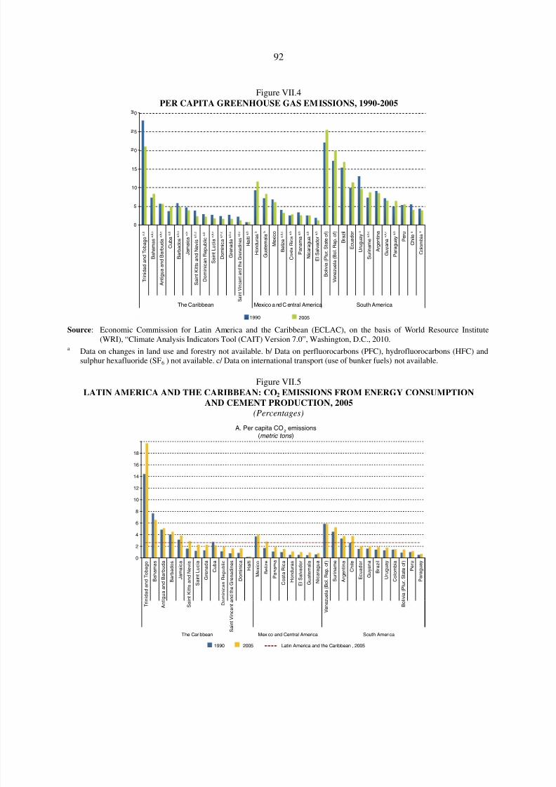
8/8/2019 CEPAL Climate Change 2010
http://slidepdf.com/reader/full/cepal-climate-change-2010 92/107
92
Figure VII.4PER CAPITA GREENHOUSE GAS EMISSIONS, 1990-2005
Source: Economic Commission for Latin America and the Caribbean (ECLAC), on the basis of World Resource Institute(WRI), “Climate Analysis Indicators Tool (CAIT) Version 7.0”, Washington, D.C., 2010.
a Data on changes in land use and forestry not available. b/ Data on perfluorocarbons (PFC), hydrofluorocarbons (HFC) andsulphur hexafluoride (SF6 ) not available. c/ Data on international transport (use of bunker fuels) not available.
Figure VII.5LATIN AMERICA AND THE CARIBBEAN: CO2 EMISSIONS FROM ENERGY CONSUMPTION
AND CEMENT PRODUCTION, 2005
(Percentages)
0
5
10
15
0
5
0
T r i n
i d a d a n d T o b a g o a , b
B a h a m a s a , b , c
A n t i g
u a a n d B a r b u d a a , b , c
C u b a a , b
B a r b a d o s a , b , c
J a m a i c a a , b
S a i n t K i t t s a n d N e v i s a , b , c
D o m i n i c a n R e p u b l i c a , b
S a i n t L u c i a a , b , c
D o m i n i c a a , b , c
G r e n a d a a , b , c
S a i n t V i n c e n t a n d t h e G r e n a d i n e s a , b , c
H a i t i a , b
H o n d u r a s b
G u a t e m a l a b
M e x i c o
B e l i z e a , b , c
C o s t a R i c a a , b
P a n a m a a , b
N i c a r a g u a a , b
E l S a l v a d o r a , b
B
o l i v i a ( P l u r . S t a t e o f )
V e n
e z u e l a ( B o l . R e p . o f )
B r a z i l
E c u a d o r
U r u g u a y a
S u r i n a m e a , b , c
A r g e n t i n a
G u y a n a a , b , c
P a r a g u a y a , b
P e r u
C h i l e a
C o l o m b i a a
The Caribbean Mexico a nd C entral America South America
1990 2005
0
2
4
6
8
10
12
14
16
18
T r i n i d a d a n d T o b a g o
B a h a m a s
A n t i g u a a n d B a r b u d a
B a r b a d o s
J a m a i c a
S a i n t K i t t s a n d N e v i s
S a i n t L u c i a
G r e n a d a
C u b a
D o m i n i c a n R e p u b l i c
S a i n t V i n c e n t a n d t h e G r e n a d i n e s
D o m i n i c a
H a i t i
M e x i c o
B e l i z e
P a n a m a
C o s t a R i c a
H o n d u r a s
E l S a l v a d o r
G u a t e m a l a
N i c a r a g u a
V e n e z u e l a ( B o l . R e p . o f )
S u r i n a m e
A r g e n t i n a
C h i l e
E c u a d o r
G u y a n a
B r a z i l
U r u g u a y
C o l o m b i a
B o l i v i a ( P l u r . S t a t e o f )
P e r u
P a r a g u a y
The Caribbean Mexico and Central America South America
1990 2005 Latin America and the Caribbean , 2005
A. Per capita CO2
emissions(metric tons )
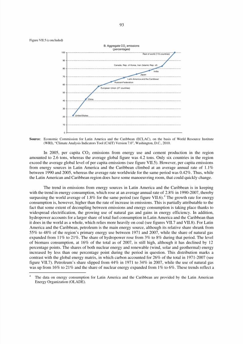
8/8/2019 CEPAL Climate Change 2010
http://slidepdf.com/reader/full/cepal-climate-change-2010 93/107
93
Figure VII.5 (concluded)
Source: Economic Commission for Latin America and the Caribbean (ECLAC), on the basis of World Resource Institute(WRI), “Climate Analysis Indicators Tool (CAIT) Version 7.0”, Washington, D.C., 2010.
In 2005, per capita CO2 emissions from energy use and cement production in the regionamounted to 2.6 tons, whereas the average global figure was 4.2 tons. Only six countries in the regionexceed the average global level of per capita emissions (see figure VII.5). However, per capita emissionsfrom energy sources in Latin America and the Caribbean climbed at an average annual rate of 1.1%between 1990 and 2005, whereas the average rate worldwide for the same period was 0.42%. Thus, whilethe Latin American and Caribbean region does have some manoeuvring room, that could quickly change.
The trend in emissions from energy sources in Latin America and the Caribbean is in keepingwith the trend in energy consumption, which rose at an average annual rate of 2.8% in 1990-2007, therebysurpassing the world average of 1.8% for the same period (see figure VII.6).4 The growth rate for energyconsumption is, however, higher than the rate of increase in emissions. This is partially attributable to thefact that some extent of decoupling between emissions and energy consumption is taking place thanks towidespread electrification, the growing use of natural gas and gains in energy efficiency. In addition,hydropower accounts for a larger share of total fuel consumption in Latin America and the Caribbean thanit does in the world as a whole, which relies more heavily on coal (see figures VII.7 and VII.8). For LatinAmerica and the Caribbean, petroleum is the main energy source, although its relative share shrank from55% to 48% of the region’s primary energy use between 1971 and 2007, while the share of natural gasexpanded from 11% to 21%. The share of hydropower rose from 3% to 8% during that period. The level
of biomass consumption, at 16% of the total as of 2007, is still high, although it has declined by 12percentage points. The shares of both nuclear energy and renewable (wind, solar and geothermal) energyincreased by less than one percentage point during the period in question. This distribution marks acontrast with the global energy matrix, in which carbon accounted for 26% of the total in 1971-2007 (seefigure VII.7). Petroleum’s share slipped from 44% in 1971 to 34% in 2007, while the use of natural gaswas up from 16% to 21% and the share of nuclear energy expanded from 1% to 6%. These trends reflect a
4 The data on energy consumption for Latin America and the Caribbean are provided by the Latin AmericanEnergy Organization (OLADE).
B. Aggregate CO2
emissions(percentages )
United States
China
European Union (27 countries)
Russian Federation
Latin America and the Caribbean
Japan
India
Canada, Rep. of Korea, Iran (Islamic Rep. of)
Rest of world (115 countries)
0
10
20
30
40
50
60
70
80
90
100
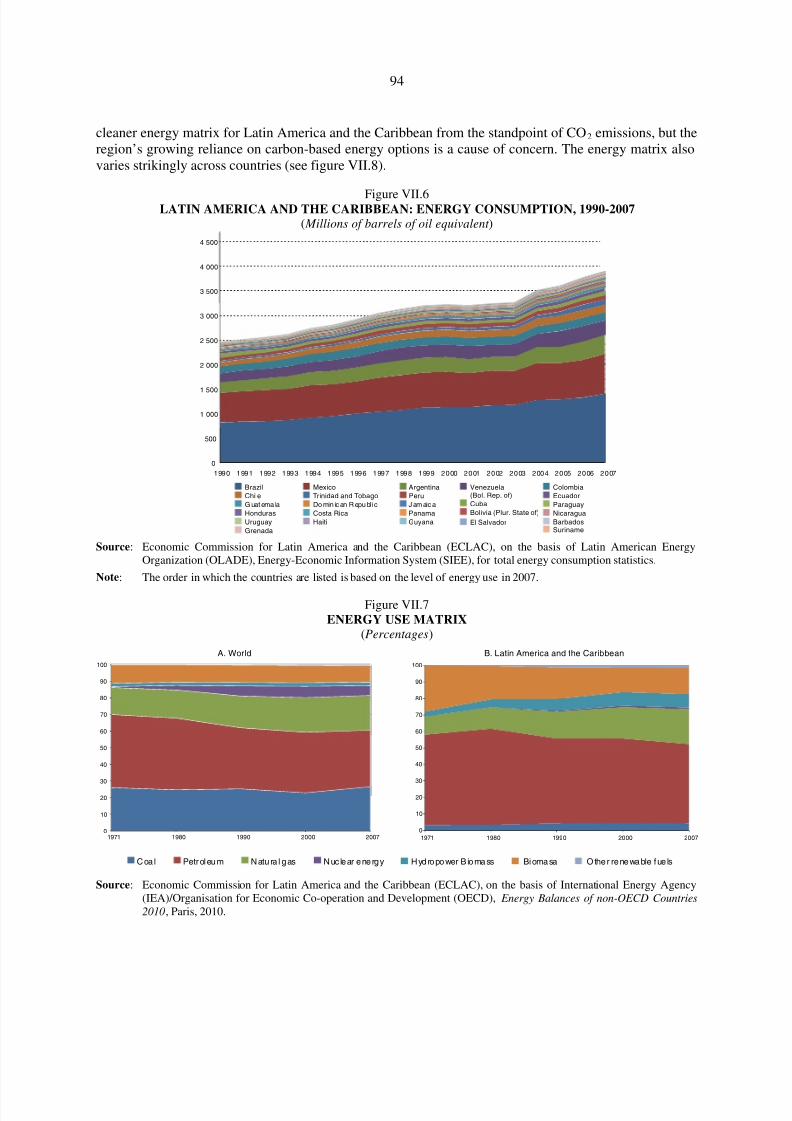
8/8/2019 CEPAL Climate Change 2010
http://slidepdf.com/reader/full/cepal-climate-change-2010 94/107
94
cleaner energy matrix for Latin America and the Caribbean from the standpoint of CO2 emissions, but theregion’s growing reliance on carbon-based energy options is a cause of concern. The energy matrix alsovaries strikingly across countries (see figure VII.8).
Figure VII.6LATIN AMERICA AND THE CARIBBEAN: ENERGY CONSUMPTION, 1990-2007
( Millions of barrels of oil equivalent )
Source: Economic Commission for Latin America and the Caribbean (ECLAC), on the basis of Latin American EnergyOrganization (OLADE), Energy-Economic Information System (SIEE), for total energy consumption statistics.
Note: The order in which the countries are listed is based on the level of energy use in 2007.
Figure VII.7ENERGY USE MATRIX
(Percentages)
Source: Economic Commission for Latin America and the Caribbean (ECLAC), on the basis of International Energy Agency(IEA)/Organisation for Economic Co-operation and Development (OECD), Energy Balances of non-OECD Countries2010, Paris, 2010.
0
500
1 000
1 500
2 000
2 500
3 000
3 500
4 000
4 500
1990 1991 1992 1993 1994 1995 1996 1997 1998 1999 2000 2001 2002 2003 2004 2005 2006 2007
Brazil Mexico Argentina Venezuela(Bol. Rep. of)
Colombia
Chile Trinidad and Tobago PeruCuba
Ecuador
G uat ema la Do min ic an R epu bli c J am aic aBolivia (Plur. State of)
Paraguay
Honduras Costa Rica Panama
El Salvador
Nicaragua
Uruguay Haiti GuyanaSurinameBarbados
Grenada
0
10
20
30
40
50
60
70
80
90
100
1971 1980 1990 2000 20070
10
20
30
40
50
60
70
80
90
100
1971 1980 1990 2000 2007
A. World B. Latin America and the Caribbean
Coal Petroleum Natura l gas Nuc lear energy Hydropower B iomass Biomasa Other renewable fue ls

8/8/2019 CEPAL Climate Change 2010
http://slidepdf.com/reader/full/cepal-climate-change-2010 95/107
95
Figure VII.8LATIN AMERICA AND THE CARIBBEAN: ENERGY MATRIX, 2007
(Percentages)
Source: Economic Commission for Latin America and the Caribbean (ECLAC), on the basis of International Energy Agency(IEA)/Organisation for Economic Co-operation and Development (OECD), Energy Balances of non-OECD Countries2010, Paris, 2010.
It is therefore important to identify the determinants of energy demand, since they are some of themost influential factors in shaping trends in the distribution of energy sources and energy intensity.Econometric estimates5 of energy demand for South America indicate that its per capita income elasticity(y) is generally high (averaging around 1), whereas its price elasticity (p) is quite low (between 0 and-0.2) (see table VII.2). These estimates also indicate that steady economic growth in the region will becoupled with an upswing in energy demand. In addition, the low price elasticity of energy demand reflectsthe fact that there are few more energy-efficient technological options available and points to thelimitations of a short-term pricing policy as a tool for curbing demand.
5 The econometric estimates were calculated using dynamic least squares (Pedroni, 2001) and panel data for SouthAmerica (Samaniego and Galindo, 2009).
0
10
20
30
40
50
60
70
80
90
100
Coal Petroleum Natural gas Nuclear energy Hydropower Biomass Biomasa Other renewablefuels
A r g e n t i n a
B r a z i l
C h i l e
C o l o m b i a
C o s t a R i c a
C u b a
E c u a d o r
E l S a l v a d o r
G u a t e m a l a
H a i t i
H o n d u r a s
J a m a i c a
M e x i c o
N i c a r a g u a
P a r a g u a y
P e r u
T r i n i d a d a n d
T o b a g o
U r u g u a y
V e n e z u e l a
( B o l . R e p . o f )
L a t i n A m e r i c a a n d
t h e C a r i b b e a n
O E C D
W o r l d

8/8/2019 CEPAL Climate Change 2010
http://slidepdf.com/reader/full/cepal-climate-change-2010 96/107
96
Table VII.2SOUTH AMERICA: ENERGY DEMAND ESTIMATES, 1985-2007
y t-stat p t-stat
Argentina 1.20 7.67 -0.02 -4.14Bolivia (Plurinational State of) 2.36 4.78 -0.01 -0.02
Brazil 1.94 8.29 -0.01 -9.16
Chile 0.99 27.44 -0.07 -4.16
Colombia 0.34 2.38 -0.15 -5.28
Ecuador 1.45 7.76 -0.07 -7.20
Paraguay 0.65 1.95 -0.22 -8.64
Peru 0.70 15.14 -0.01 -6.71
Uruguay 0.63 4.68 -0.03 -3.18
Venezuela (Bolivarian Republic of) 0.36 2.28 -0.11 -17.25
Group 1.06 26.04 -0.07 -20.79
PEDRONI PANEL COINTEGRATION TEST
Statistic Coefficient P-value
Panel – V 3.03 0.00
Panel – rho -0.15 0.44
Panel – PP -1.85 0.03
Panel – ADF -1.96 0.03
Group – rho 0.80 0.21
Group – PP -1.86 0.03
Group – ADF -1.97 0.02
Source: Economic Commission for Latin America and the Caribbean (ECLAC), on the basis of Latin American EnergyOrganization (OLADE), Energy-Economic Information System (SIEE), for total energy consumption statistics andprices; and ECLAC, Economic Indicators and Statistics Database (BADECON) for GDP at constant 2000 prices.
Note: The reported values are distributed as a standard normal [N(0,1)] under the null hypothesis of a unit root or of nocointegration. PP: Phillips-Perron; ADF: Augmented Dickey-Fuller.
The available evidence for Latin America and the Caribbean also indicates that, as in all moderneconomies, per capita emissions, per capita energy consumption and per capita GDP are closely correlated(see figures VII.9 and VII.10). Countries with higher per capita incomes also have higher levels of per capita
energy consumption and per capita emissions. Evidence also shows that, generally speaking, energyconsumption is gradually decoupling from per capita GDP (see figure VII.11). The extent of energydecoupling is not yet sufficient to halt the rise in energy consumption in Latin America and the Caribbean,however, and the current style of growth still demands a great deal of energy. For this reason, sharp decreasein energy consumption would therefore have a negative impact on the region’s growth rate.

8/8/2019 CEPAL Climate Change 2010
http://slidepdf.com/reader/full/cepal-climate-change-2010 97/107
97
Figure VII.9LATIN AMERICA AND THE CARIBBEAN: PER CAPITA ENERGY CONSUMPTION AND GDP, 2007
(Thousands of barrels of oil equivalent and dollars)
Source: Economic Commission for Latin America and the Caribbean (ECLAC), on the basis of Latin American EnergyOrganization (OLADE), Energy-Economic Information System (SIEE), for total energy consumption statistics; andWorld Bank for per capita GDP data (valued at purchasing power parity in 2005 dollars.
Figure VII.10LATIN AMERICA AND THE CARIBBEAN: PER CAPITA GDP AND PER CAPITA
ENERGY CONSUMPTION, 2007 ( Barrels of oil equivalent and dollars)
Source: Economic Commission for Latin America and the Caribbean (ECLAC), on the basis of Latin American EnergyOrganization (OLADE), Energy-Economic Information System (SIEE), for total energy consumption statistics; andWorld Bank for per capita GDP data valued at purchasing power parity in 2005 dollars.
ARG
BOL
BRA
CHLCOL
CRIECUSLV
GRD
GTM
GUY
HTIHND JAM
MEX
NICPAN
PRY
PER
SUR URY
VEN
0
500 000
1 000 000
1 500 000
0 5 000 10 000 15 000
ARG
BOL
BRA
CHL
COL
CRI
DOM
ECU
SLV
GRD
GTM
GUY
HTI
HND
JAM
MEX
NIC
PAN
PRY
PER
SUR
URY
VEN
2
4
6
8
10
0 5 000 10 000 15 000
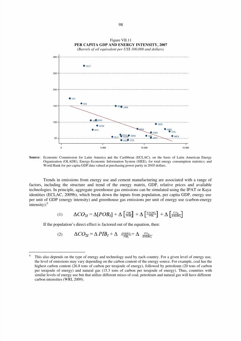
8/8/2019 CEPAL Climate Change 2010
http://slidepdf.com/reader/full/cepal-climate-change-2010 98/107
98
Figure VII.11PER CAPITA GDP AND ENERGY INTENSITY, 2007
(Barrels of oil equivalent per US$ 100,000 and dollars)
Source: Economic Commission for Latin America and the Caribbean (ECLAC), on the basis of Latin American EnergyOrganization (OLADE), Energy-Economic Information System (SIEE), for total energy consumption statistics; andWorld Bank for per capita GDP data valued at purchasing power parity in 2005 dollars.
Trends in emissions from energy use and cement manufacturing are associated with a range of factors, including the structure and trend of the energy matrix, GDP, relative prices and availabletechnologies. In principle, aggregate greenhouse gas emissions can be simulated using the IPAT or Kayaidentities (ECLAC, 2009b), which break down the inputs from population, per capita GDP, energy useper unit of GDP (energy intensity) and greenhouse gas emissions per unit of energy use (carbon-energyintensity):6
(1)
If the population’s direct effect is factored out of the equation, then:
(2)
6 This also depends on the type of energy and technology used by each country. For a given level of energy use,the level of emissions may vary depending on the carbon content of the energy source. For example, coal has thehighest carbon content (26.8 tons of carbon per terajoule of energy), followed by petroleum (20 tons of carbonper terajoule of energy) and natural gas (15.3 tons of carbon per terajoule of energy). Thus, countries withsimilar levels of energy use but that utilize different mixes of coal, petroleum and natural gas will have differentcarbon intensities (WRI, 2009).
ARGBOL BRACHL
COL
CRIDOMECU
SLVGRD
GTM
GUY
HTI
HND
JAM
MEX
NIC
PAN
PRY
PER
SUR
URY
VEN
50
100
150
200
250
300
0 5 000 10 000 15 000

8/8/2019 CEPAL Climate Change 2010
http://slidepdf.com/reader/full/cepal-climate-change-2010 99/107
99
It is therefore reasonable to expect that more economic growth and/or an increase in thepopulation will drive up emissions, as well as energy consumption. It is also feasible, however, that agradual process of energy decoupling (ratio of energy to GDP) and decarbonization (ratio of emissions toenergy) may occur in economies with high per capita incomes. As may be seen from figure VII.12, the
distribution of these variables is very heterogeneous at the country level, reductions in energy intensity, atan average annual rate for the region of -0.3%, are more frequent than reductions in emissions intensity inrelation to energy, which has, on average, remained virtually constant.
Figure VII.12LATIN AMERICA AND THE CARIBBEAN: AVERAGE ANNUAL INCREASE IN CO2
EMISSIONS AND ASSOCIATED FACTORS, 1990-2005(Percentages)
Source: Economic Commission for Latin America and the Caribbean (ECLAC), on the basis of World Resources Institute(WRI), “Climate Analysis Indicators Tool (CAIT) Version 7.0”, 2010; Latin American Energy Organization (OLADE),Energy-Economic Information System (SIEE); World Bank; and Social Indicators and Statistics Database(BADEINSO) of ECLAC.
Note: Countries for which data on energy use are unavailable are not shown.
0.0
0.5
1.0
1.5
2.0
-1
-2
0
1
2
3
0
4
3
2
1
0
A. Population
ARG
BO L
BR A
CHL
COL
CRI
EC U
SLV
GRD
GT M
GUY
HND
JAM
ME X
NIC
PA N
PRY
PER
DOM
SU R
TTOURY
VEN
B. Per capita GDP
AR G
BO L
BR A
CHL
COL
CRI
EC U
SL V
GRD
GT M
GUY
HND
JAM
ME XNIC
PA N
PRY
PER
DOM
SUR
TT O
URY
VEN
C. Energy intensity
AR GBO L
BR A
CHL
COL
CRI
EC U
SL V
GRD
GT M
GUY
HND
JAM
ME X
NI C
PA N
PRY
PER
DOMSU R
TT O
URY
VE N
Latin America and the Caribbean (-0.3%)
−4
−2
2
4
ARG
BO L
BR A
CHL
COL
CRI
ECU
SL V
GRD
GTM
GUY
HND
JAM
ME XNI C
PAN
PRY
PERDOM
SU R
TT O
URY
VEN
Latin America and the Caribbean (1.6%)
Latin America and the Caribbean (-0.01%)
Latin America and the Caribbean (-1.5%)
D. Carbon intensity
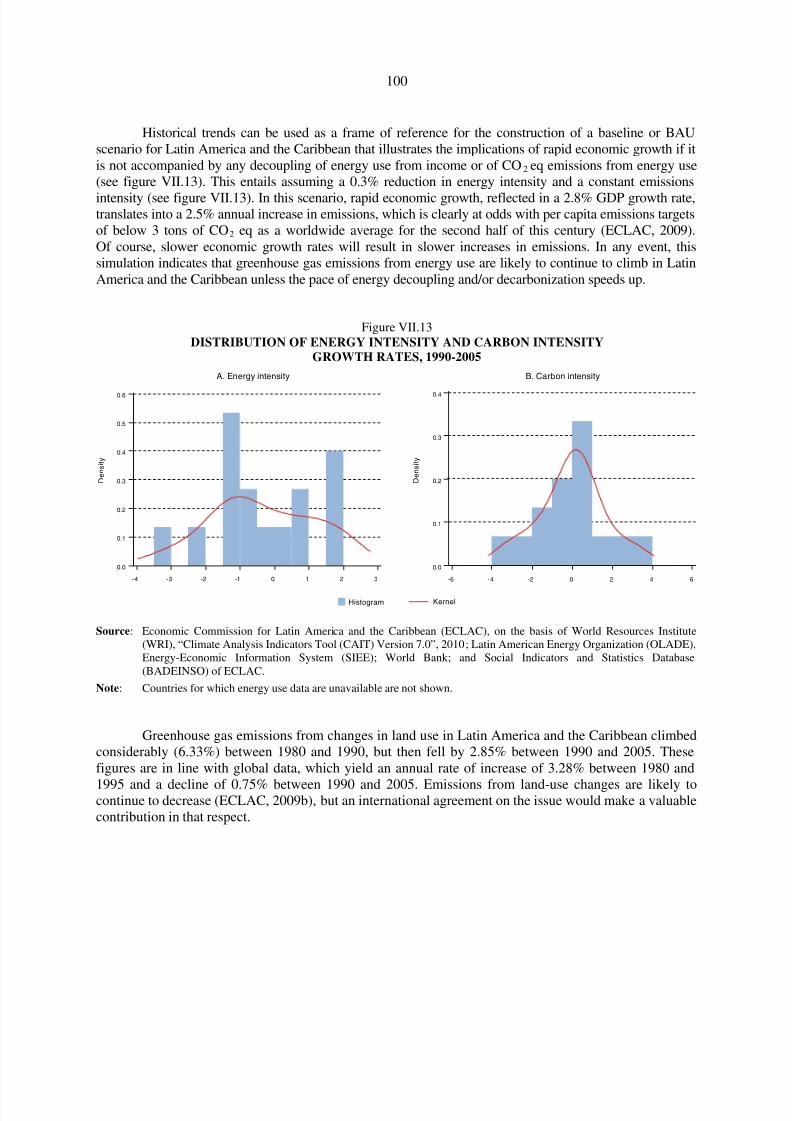
8/8/2019 CEPAL Climate Change 2010
http://slidepdf.com/reader/full/cepal-climate-change-2010 100/107
100
Historical trends can be used as a frame of reference for the construction of a baseline or BAUscenario for Latin America and the Caribbean that illustrates the implications of rapid economic growth if itis not accompanied by any decoupling of energy use from income or of CO2 eq emissions from energy use(see figure VII.13). This entails assuming a 0.3% reduction in energy intensity and a constant emissions
intensity (see figure VII.13). In this scenario, rapid economic growth, reflected in a 2.8% GDP growth rate,translates into a 2.5% annual increase in emissions, which is clearly at odds with per capita emissions targetsof below 3 tons of CO2 eq as a worldwide average for the second half of this century (ECLAC, 2009).Of course, slower economic growth rates will result in slower increases in emissions. In any event, thissimulation indicates that greenhouse gas emissions from energy use are likely to continue to climb in LatinAmerica and the Caribbean unless the pace of energy decoupling and/or decarbonization speeds up.
Figure VII.13DISTRIBUTION OF ENERGY INTENSITY AND CARBON INTENSITY
GROWTH RATES, 1990-2005
Source: Economic Commission for Latin America and the Caribbean (ECLAC), on the basis of World Resources Institute(WRI), “Climate Analysis Indicators Tool (CAIT) Version 7.0”, 2010; Latin American Energy Organization (OLADE),Energy-Economic Information System (SIEE); World Bank; and Social Indicators and Statistics Database(BADEINSO) of ECLAC.
Note: Countries for which energy use data are unavailable are not shown.
Greenhouse gas emissions from changes in land use in Latin America and the Caribbean climbedconsiderably (6.33%) between 1980 and 1990, but then fell by 2.85% between 1990 and 2005. Thesefigures are in line with global data, which yield an annual rate of increase of 3.28% between 1980 and
1995 and a decline of 0.75% between 1990 and 2005. Emissions from land-use changes are likely tocontinue to decrease (ECLAC, 2009b), but an international agreement on the issue would make a valuablecontribution in that respect.
0.0
0.1
0.2
0.3
0.4
0.5
0.6
-4 -3 -2 -1 0 1 2 3
0.0
0.1
0.2
0.3
0.4
-6 -4 -2 0 2 4 6
D e n s i t y
Histogram
A. Energy intensity B. Carbon intensity
Kernel
D e n s i t y

8/8/2019 CEPAL Climate Change 2010
http://slidepdf.com/reader/full/cepal-climate-change-2010 101/107
101
The main messages, therefore, are as follows:
Trends in atmospheric greenhouse gas concentrations and emissions for this century indicate that,with a high degree of probability, the temperature will rise by 2oC by 2050 and by 3oC or even 4oC by the
century’s end. If the most extreme climate-change scenarios are to be avoided, a global mitigationstrategy will have to be put in place that recognizes the countries’ common but differentiatedresponsibilities. Such a strategy should aim at attaining average per capita global emissions levels of between 2 and 3 tons of CO2 eq (Hepburn and Stern 2008).
The evidence shows that the Latin American and Caribbean region accounts for a small portion of global emissions and has a cleaner-than-average energy matrix, but a large part of its emissions comefrom deforestation. The rate of increase of total greenhouse gases for the region, at 1.19% for 1990-2005,is similar to the worldwide average, but is higher when fossil-fuel emissions are considered in isolation.In addition, at the country level, emissions levels in Latin America and the Caribbean are very uneven andare much higher in certain countries.
Energy consumption in Latin America and the Caribbean has risen at a higher average annual ratethan emissions from energy use, which points to a slight extent of energy decoupling. Energy demandestimates also reflect a high income elasticity and very low price elasticity. This indicates that continuedeconomic growth in the region will go hand in hand with a heavier demand for energy, while the lowprice elasticity of energy demand suggests that a pricing policy has limited potential as a tool fordampening energy consumption. The evidence for Latin America and the Caribbean shows that per capitaemissions, per capita energy consumption and per capita GDP are closely correlated. It also points to amarginal process of energy decoupling, but one that is not yet strong enough to halt the growth of energyuse in Latin America and the Caribbean.
Energy emissions projections indicate that, if historical trends in energy and emissions continuealong the same trajectory and if the region’s economy grows rapidly, then its energy emissions will do so
as well. Emissions associated with land-use changes are, on the other hand, diminishing, and aninternational agreement on this issue could help lead to further reductions.
VIII. CONCLUSIONS
Scientific evidence indicates that the global warming associated with increased greenhouse gas (GHG)emissions from anthropogenic activity is bringing about appreciable climatic changes. The evidence of climate change in Latin America and the Caribbean is in line with the available evidence at theinternational level, although some significant regional differences do exist.
The point of departure for an analysis of the economics of climate change is the definition of abusiness-as-usual (BAU) baseline that can be used as a point of reference for comparisons with estimatesof the economic impacts of probable climate-change scenarios —in this study, B2 (moderate change) andA2 (more radical change)— and of the economic implications of adaptation and mitigation processes.Economic growth in Latin America has generally trended upward, but with oscillations around the trendline, together with structural changes in the mean growth path. Although there is no absolute convergenceof the per capita GDP growth trends of the Latin American countries, given the presence of differentiatedtrends by decade and group of countries, this does not rule out the possibility of conditional convergence.
8/8/2019 CEPAL Climate Change 2010
http://slidepdf.com/reader/full/cepal-climate-change-2010 102/107
102
These regular patterns make it possible to identify long-term socioeconomic scenarios in which there is ahigh degree of probability that per capita GDP growth will stand at about 1.7% per year.
The projected trend and path of global GHG concentrations (stocks) and emissions (flows) for
this century point, with a high degree of probability, to a rise in temperature of 2ºC by 2050 and of 3ºC oreven 4ºC by its end. Climate projections for Latin America and the Caribbean also indicate that there willbe a gradual but unremitting increase in average temperatures, although with differences from one part of the region to the next, and that there will also be changes in the amount, intensity and frequency of precipitation. The records also indicate that sea levels are rising, particularly in the Gulf of Mexico andthe Caribbean Sea. Growing climatic variability is, in addition, leading to an increase in extreme weatherevents. Projections for South America for this century signal a progressive rise in the mean temperature of between 1°C and 4°C under the low-emissions (B2) scenario and of between 2°C and 6°C under thehigher-emissions (A2) scenario.
The empirical evidence for Latin America and the Caribbean indicates that, in the aggregate,these changes in the climate are having significant impacts on the region’s economies and that these
effects will become stronger as time goes on. Added pressure on the region’s water resources, increasedforest fires, slumps in agricultural productivity in some areas, negative health impacts, the damage thatwill be sustained in coastal areas as sea levels rise, diminished ecosystem services as a consequence of serious losses of biodiversity, the higher morbidity and mortality levels associated with extreme weatherevents and other impacts will be an additional source of concern for the region and will alter itsdevelopment path. These effects will also, however, differ across climatic zones, areas, sectors andeconomic agents and, over time, will exhibit non-linear patterns and specific thresholds. Preliminaryestimates of the economic costs and benefits of climate change for Latin America and the Caribbean,based on the available information, nonetheless indicate that the overall effect will be negative and willincrease over time. Countries in temperate zones may lose as much as roughly 1% of annual GDPthroughout the reference period (up to the year 2100 under scenario A2), which exceeds the entirebudgets of these nations’ ministries of the environment. The costs are likely to be higher in the Andean,
Central American and Caribbean countries. Furthermore, in some cases, such as those in which climatechange has an impact on biodiversity or human life, there will be irreversible consequences that cannot bequantified in economic terms. How dramatic or how tolerable the situation will be will depend on whathappens in terms of emissions levels. Clearly, however, the climate-change processes already under waymake adaptation inevitable.
If the most extreme climate-change scenarios are to be averted, a global mitigation strategyentailing common but differentiated responsibilities will have to be launched in order to reduce averageglobal per capita emissions levels to between 2 and 3 tons of carbon dioxide equivalent (CO 2 eq). In thenear future, the Latin American and Caribbean region’s emissions levels will surpass that benchmark unless mitigation measures are put in place, even though the region accounts for a relatively smallpercentage of total global emissions and has a relatively cleaner energy matrix, with much of its
emissions coming from changes in land use (mainly deforestation). The emissions associated with energyconsumption continue to climb, however, while emissions from land-use changes (deforestation) arewaning. Emissions profiles also differ markedly across countries.
Available evidence shows that emissions from energy use account for a small percentage of totalemissions worldwide but are rising steeply. This situation is reflected, for example, in the fact that energydemand has a high income elasticity but a very low price elasticity. This means that continued economicgrowth in the region will be coupled with an upswing in energy demand, while the low price elasticity of the demand for energy would seem to indicate that pricing policy may be of limited usefulness as a tool
8/8/2019 CEPAL Climate Change 2010
http://slidepdf.com/reader/full/cepal-climate-change-2010 103/107
103
for curbing energy consumption in the short run. Evidence for Latin America and the Caribbean alsopoints to a close correlation among per capita emissions, per capita energy consumption and per capitaGDP and to a marginal process of energy decoupling, although it is not yet strong enough to halt theincrease in energy consumption.
If past trends in energy intensity and in the carbon intensity of energy use continue unchangedand if the region experiences rapid economic growth, the emissions from energy use will also continue toclimb sharply. This scenario is at odds with per capita emissions targets of between 2 and 3 tons of CO 2
eq. The countries of the region do, however, have a wide range of low-cost mitigation opportunities, someof which can afford actual reductions. These opportunities are also associated with a number of significant co-benefits, especially for lower-income groups.
The magnitude of the impacts associated with changed climatic conditions and the extent of theeffort involved in decoupling the economic growth path from energy consumption and emissionsrepresent an additional development constraint that can only be overcome by mounting a major adaptationeffort and transitioning to a low-carbon, equality-based economy. If the region is to decrease its high
degree of socioeconomic and environmental vulnerability to the effects of climate change, it will have toredouble its efforts to reduce poverty and inequality, boost its resilience and enhance the capacity of itssocieties and ecosystems to adapt to the observed and expected changes in the climate.
Investment in adaptation should be an economic and social development priority. The firstquestion that the region must resolve is how to determine the amount of resources that it should devote tothe design, planning and implementation of adaptation policies, how it should invest those resources andhow it should allocate the associated costs. Adaptation entails a wide range of actions in connection withthe various sectors and areas of economic activity, lifestyles, risk management, and ecosystems andnatural resources.
Both the causes and the consequences of climate change are a global problem which, viewed
from an economic vantage point, constitutes a global negative externality. Solving this problem willincrease the general level of well-being, but this does not mean that certain groups or regions will not seea decline in well-being, for which they can be properly compensated. An economically sound global risk-management strategy therefore needs to be designed and implemented that recognizes countries’ commonbut differentiated responsibilities. The economic costs associated with climate-change impacts are higherfor the Latin American and Caribbean countries as a group than the costs of taking part in mitigationagreements that recognize historical responsibilities and set regionally differentiated targets in accordancewith the principles of equity and co-responsibility.
A sustainable, adaptive, low-carbon, socially inclusive development strategy must therefore bedesigned and implemented. This strategy must be based on an awareness that forms of economic growththat do not take into account climate-related phenomena and considerations of equality will carry a high
level of risk that is quite likely to prove to be unsustainable in the long run. Studies of the economics of climate change for the countries of the region make up part of this effort.

8/8/2019 CEPAL Climate Change 2010
http://slidepdf.com/reader/full/cepal-climate-change-2010 104/107

8/8/2019 CEPAL Climate Change 2010
http://slidepdf.com/reader/full/cepal-climate-change-2010 105/107
105
Bibliography
Aguilar, E. and others (2005), “Changes in precipitation and temperature extremes in Central America
and Northern South America, 1961-2003”, Journal of Geophysical Research, vol. 110.Agrawala, S. and S. Fankhauser (2008), Economic Aspects of Adaptation to Climate Change: Costs,
Benefits and Policy Instruments, Paris, OECD Publishing.Barro, Robert J. and Xavier Sala-i-Martin (2009), Crecimiento económico, Barcelona, Editorial Reverté.
(1992), “Convergence”, Journal of Political Economy, vol. 100, No. 2.Baumert, K.A., T. Herzog and J. Pershing (2005), Navigating the Numbers: Greenhouse Gas Data and
International Climate Policy, Washington, D.C., World Resources Institute (WRI).Blanchard, Olivier (1997), “Is there a core of usable macroeconomics?”, American Economic Review,
vol. 87, No. 2, May.Britton, E., P. Fisher and J. Whitley (1998), “The inflation report projections: understanding the fan
chart”, Bank of England Quarterly Bulletin, vol. 38, No. 1, February.Brooks, Chris (2002), Introductory Econometrics for Finance, Cambridge University Press.
Canova, F. (2007), Methods for Applied Macroeconomic Research, Princeton University Press.(1998), “Detrending and business cycle facts”, Journal of Monetary Economics, vol. 41, No. 3,
20 May.Christensen, J.H. and A.B. Hewitson (2007), “Regional climate projections”, Climate Change 2007: the
Physical Science Basis. Contribution of Working Group I to the Fourth Assessment Report of the IPCC , Cambridge University Press.
Church, A.J. and N.J. White (2006), “A 20th century acceleration in global sea-level rise”, Geophysical Research Letters, vol. 33, No. 1.
Clements, Michael P. and David F. Hendry (2004), “Pooling of forecasts”, The Econometrics Journal,vol. 7, No. 1.
De Gregorio, José and Jong-Wha Lee (2003), “Growth and adjustment in East Asia and Latin America”,Central Bank of Chile Working Papers, No. 245, December.
Easterling, William E. and others (1993), “Agricultural impacts of and responses to climate change in theMissouri-Iowa-Nebraska-Kansas (MINK) region”, Climatic Change, vol. 24, No. 1-2.
ECLAC (Economic Commission for Latin America and the Caribbean) (2010a), “La economía del cambioclimático en Uruguay. Síntesis”, Project documents, No. 330 (LC/W.330), Santiago, Chile.(2010b), “La economía del cambio climático en Centroamérica”, Project documents, forthcoming.(2009a) “La economía del cambio climático en Chile. Síntesis”, Project documents , No. 288
(LC/W.288), Santiago, Chile.(2009b), Economics of climate change in Latin America and the Caribbean. Summary 2009
(LC/G.2425), Santiago, Chile, November.Fischer, Stanley (1993), “The role of macroeconomic factors in growth”, Journal of Monetary
Economics, vol. 32, No. 3.Fankhauser, Samuel (1995), Valuing Climate Change: The Economics of the Greenhouse Effect ,
Earthscan Publications.Galindo, L.M. (2009), La economía del cambio climático en México. Síntesis, Mexico City, Secretariat of
the Environment and Natural Resources (SEMARNAT).Hamilton, James Douglas (1994), Time Series Analysis, Princeton University Press, January.Hepburn, C. and N. Stern (2008), “A new global deal on climate change”, Oxford Review of Economic
Policy, vol. 24, No. 2.Hodrick, R.J. and E.C. Prescott (1997), “Postwar U.S. business cycles: an empirical investigation”,
Journal of Money, Credit and Banking, vol. 29, No. 1.

8/8/2019 CEPAL Climate Change 2010
http://slidepdf.com/reader/full/cepal-climate-change-2010 106/107
106
IPCC (Intergovernmental Panel on Climate Change) (2007a), Climate Change 2007: the Physical Science Basis. Contribution of Working Group I to the Fourth Assessment Report of the IPCC ,Cambridge University Press.(2007b), Climate Change 2007: Impacts, Adaptation and Vulnerability. Contribution of Working
Group II to the Fourth Assessment Report of the IPCC , Cambridge University Press.(2007c), Climate Change 2007: Impacts and Vulnerability. Contribution of Working Group II to
the Fourth Assessment Report of the IPCC.. Summary for policy-makers , M.L. Parry and others(eds.), Cambridge University Press.(2001), “IPCC Third Assessment Report - Climate Change 2001 - Complete online versions /
UNEP/GRID-Arendal - Publications - Other” [online] http://www.grida.no/publications/other/ ipcc_tar/ [date of reference: 10 November 2010].(1995), Second Assessment Report: Climate Change , Geneva.
Julio, Juan Manuel (2007), “The fan chart: the technical details of the new implementation”, Borradoresde economía, No. 468, Bogota, Banco de la República.
Kaiser, Regina and Agustín Maravall (1999), “Short-term and long-term trends, seasonal adjustment, andthe business cycles”, Banco de España Working Papers, No. 9918.
Kiktev, D. and others (2003), “Comparison of modeled and observed trends in indices of daily climateextremes”, Journal of Climate, vol. 16, No. 22.
King, R.G. and R. Levine (1993), “Finance and growth: Schumpeter might be right”, Quarterly Journalof Economics, vol. 108, No. 3.
Maddala, G.S. and In-Moo Kim (1998), Unit Roots, Cointegration, and Structural Change, CambridgeUniversity Press.
Madden, R.A. and J. Williams (1978), “The correlation between temperature and precipitation in theUnited States and Europe”, Monthly Weather Review, vol. 106.
Magrin, G. and others (2007), “Latin America”, Climate Change 2007: Impacts, Adaptation and Vulnerability. Contribution of Working Group II to the Fourth Assessment Report of the IPCC ,Cambridge University Press.
Mankiw, N. Gregory, David Romer and David N. Weil (1992), “A contribution to the empirics of
economic growth”, Quarterly Journal of Economics, vol. 107, No. 2, May.Maravall, A. (1999), “Short-term analysis of macroeconomic time series”, Economics Beyond the
Millennium, A. Kirman and L.A. Gérard-Varet (eds.), Oxford University Press.Marengo, J.A. and others (2009a), “An intercomparison of observed and simulated extreme rainfall and
temperature events during the last half of the twentieth century. Part 2: historical trends”,Climatic Change, vol. 98, No. 3-4.(2009b), “Future change of temperature and precipitation extremes in South America as derived
from the PRECIS regional climate modeling system”, International Journal of Climatology,vol. 29, No. 15.
Meehl, G.A. and T.F. Stocker (2007), “Global climate projections”, Climate Change 2007: the PhysicalScience Basis. Contribution of Working Group I to the Fourth Assessment Report of the IPCC ,Cambridge University Press.
Mills, T.C. (2003), Modelling Trends and Cycles in Economic Time Series, Basingstoke, PalgraveMacmillan.(1991), Time Series Techniques for Economists, Cambridge University Press, June.
NOAA (National Oceanic and Atmospheric Administration) (2010), “Trends in Atmospheric CarbonDioxide” [online] http://www.esrl.noaa.gov/gmd/ccgg/trends/#global [date of reference:5 October 2010].
Nordhaus, D.W. (2008), A Question of Balance: Economic Modeling of Global Warming, New Haven,Yale University Press.
8/8/2019 CEPAL Climate Change 2010
http://slidepdf.com/reader/full/cepal-climate-change-2010 107/107