


Bahasa
Halaman
Hukum

Technical Report No. 24 ��
INDICATORS FOR DROUGHT CHARACTERIZATION ON A GLOBAL SCALE
���������� ������������������������������������������������������ �������� ���!"�"��
Technical Report No. 24 - ii -
��#$�� ��� �� %���&����� '��(���� ������� �� ���� )���*��� $�������� ������ ���� +�,��� ���-����'��&�����./� /�$��&�����)���������#������'������������0���������� �� �"123425���#�����$��*��(�����������"�6"!6!""7����-�//����������8���4�������
Title: Indicators for drought characterization on a global scale
Authors: ��������������������������������9������������������
Organisations: �&����&���:����������;������/�&�����<���������������=�&�����.���*�0�:>5����
Submission date: ������� ���!"�"��
Function: #������*���� ��������*���8��������?/����4@�#���4�!�������&������8/����������������88��������/�����
Deliverable ��#$����/���� /�����4�!���>�*���������������8�����88��������*���8�����&�������8/���������88��������/�����
�
Technical Report No. 24 - iii -
Preface ������������������� ������������ ������� ���������� �������������������� � ������������������������������������ ������ !"#$� ��� ���������������%��������&� ���������������� � � ����� ��������������� ����� � ������������������'���������������(����� ��������(����� ���)����*'�����+ ����������� )','� ���� +����'� -�� ���� � ���.�� �� ���� ���� ��������&� ���� ������ ���� �� (������(����� ��� ����-�������� ���� � ���� (� �� ��� � ������ /.������� ���� +����������� 0���&� 1�� � �� �2�$&� 34�35�*������ 6 3 '���� ����� ��(��������� �� �� ���� ������ �� �� ����78((���9��������(� ����� �������������� ������������(��� ������� ��������� ���� ������ ������ ������������� ������ �������2 ���'������������ �1�� �2�����(( ����������/%�*:#�(� ;�����)�<����)���������� ���<�����$'���
�����)','�����+����&�����������&���(������6 3 '�

Abstract
Droughts are caused by a situation with less than normal water availability due to climate variability.They occur in every hydroclimatic region and in all components of the hydrological cycle. Droughts canbe classified either as meteorological, soil moisture or hydrological drought. Identification of droughtson a global scale has been done in recent studies. Different drought indicators were used for the iden-tification of droughts on a global scale. However, the effect of the choice for a certain indicator on thedrought characterization (e.g. severity, frequency and duration of droughts) is not fully understood, asis the impact of hydroclimate and physical catchment structure. The objective of this study is to exam-ine the characterization of drought with different drought indicators across the world. It also includesthe impact of climate and physical catchment structure on the performance of the drought indicators.Time series of meteorological variables were retrieved from or calculated with the WATCH Forcing Data(WFD) at a daily time step, for cells with a resolution of 0.5◦ by 0.5◦. The NUT DAY model was appliedto generate time series of hydrological variables (e.g. soil moisture storage, discharge). NUT DAY is asynthetic rainfall-runoff model which uses precipitation, temperature and potential evapotranspirationtime series from WFD as input. Three different soil types (low, medium and high soil moisture storagecapacity) and groundwater systems types (fast, medium and slow responding) have been used in themodel simulations, to explore the effect of changes in the physical catchment structure. climatic regionswere defined with the Koppen-Geiger classification. For all climatic regions drought analyses were done.Per cell, drought events for each drought indicator were identified by applying the threshold methodto the time series of meteorological, soil moisture and hydrological variables. The threshold is eithervariable or fixed, depending on the indicator. In this study 14 indicators were selected, of which 2 werenewly developed (Moving Average Precipitation, Standardized Streamflow Index). All 14 indicators wereapplied to the 5 major climates; performances were tested and evaluated with expert knowledge mainlyfrom literature. From this 14 indicators finally 6 have been selected, for a more detailed analysis. Intotal 961 cells were randomly selected for that purpose ensuring that all Kopen-Geiger climate regionsare adequately represented. The 6 selected indicators are: the Standardized Precipitation Index (SPI),Effective Drought Index (EDI), Total Storage Deficit Index (TSDI), Moving Average Precipitation withVariable Threshold (MAPVT), Soil moisture with Variable Threshold (SVT), Discharge with VariableThreshold (QVT). These indicators were used to study the effects of hydroclimate and physical catch-ment structure on drought characterization and subsequently to assess their performance. It was foundthat the hydroclimate has a profound impact on the average drought durations and deficit volumes asidentified by all indicators. The SPI, EDI and MAPVT are not influenced by the physical catchmentstructure, because they only depend on precipitation. Average drought durations and deficit volumesdetermined by the TSDI and QVT increase for slower responding groundwater systems. In general, ahigher soil water storage capacity increases the average drought durations as identified by the TSDI, SVTand QVT. Overall, the effects of hydroclimate and of properties of the groundwater system are moreprofound than changes in soil type. The MAPVT and QVT seem to be the most promising indicatorsfor drought analysis on a global scale. Both indicators had a very constant performance for differenthydroclimates and physical catchment structures and are rather straight forward to calculate.
Keywords: Drought, Hydrology, Drought indicators, Global scale, Hydroclimate, Physical catchmentstructure
Technical Report No. 24 -iv-

LIST OF TABLES
VII.1Number of droughts per combined drought indicator for all five major climate types. . . . xviiVII.2Average duration of droughts per combined drought indicator in days for all five major
climate types. . . . . . . . . . . . . . . . . . . . . . . . . . . . . . . . . . . . . . . . . . . . xviiVII.3Average deficit volumes of droughts per combined drought indicator for all five major
climate types. . . . . . . . . . . . . . . . . . . . . . . . . . . . . . . . . . . . . . . . . . . . xviiIX.1 Mean number of droughts in days, for six selected drought indicators, all climate types,
average soil and a j-factor of 250 days (1958-2002). . . . . . . . . . . . . . . . . . . . . . . xxiIX.2 Mean deficit volumes of droughts, for six selected drought indicators, all climate types,
average soil and a j-factor of 250 days (1958-2002). . . . . . . . . . . . . . . . . . . . . . . xxiiX.1 Mean number of droughts, for two selected drought indicators, all climate types, an average
soil and different values of the j-factor (1958-2002). . . . . . . . . . . . . . . . . . . . . . . xxiiiX.2 Mean deficit volumes of droughts, for two selected drought indicators, all climate types,
an average soil and different values of the j-factor (1958-2002). . . . . . . . . . . . . . . . xxivXI.1 Mean number of droughts, for three selected drought indicators, all climate types, j-factor
of 250 days and different soil types, Coarse Sand (CS), Light Silty Loam (LSL), SandyLoam (SL)(1958-2002). . . . . . . . . . . . . . . . . . . . . . . . . . . . . . . . . . . . . . . xxv
XI.2 Mean deficit volumes of droughts, for three selected drought indicators, all climate types,j-factor of 250 days and different soil types, Coarse Sand (CS), Light Silty Loam (LSL),Sandy Loam (SL)(1958-2002). . . . . . . . . . . . . . . . . . . . . . . . . . . . . . . . . . . xxvi
-x- Technical Report No. 24
1 INTRODUCTION
1 Introduction
Background
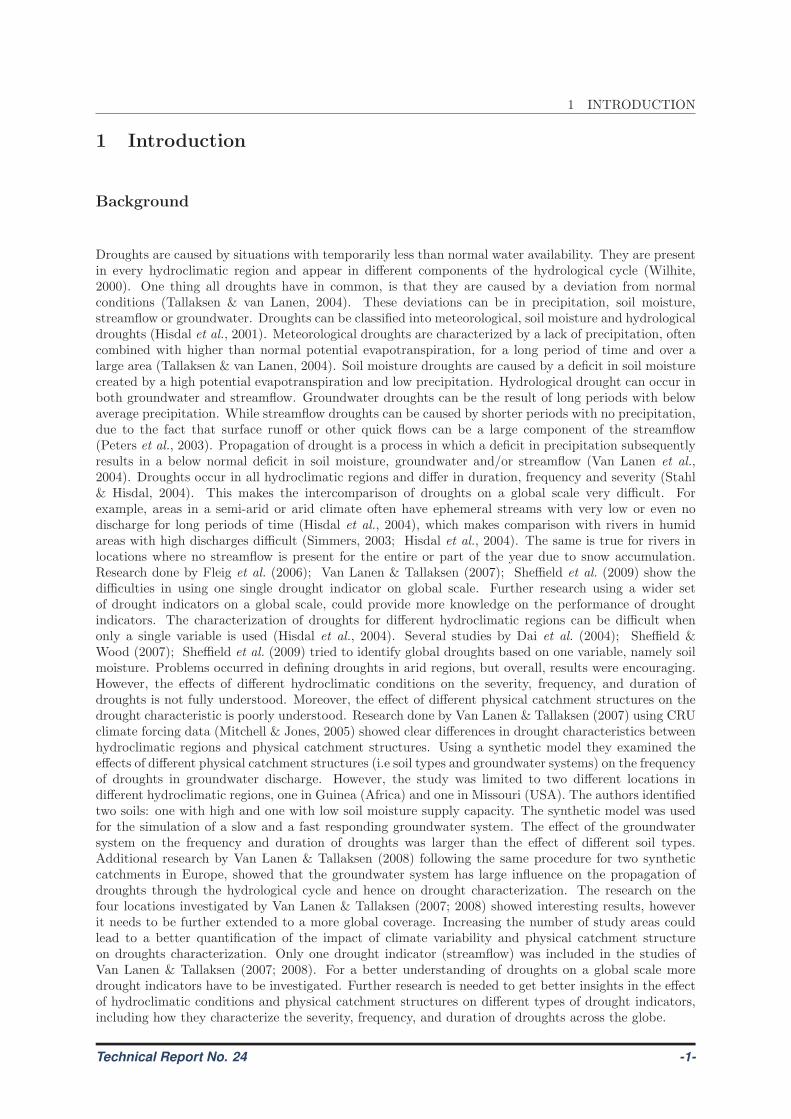
Droughts are caused by situations with temporarily less than normal water availability. They are presentin every hydroclimatic region and appear in different components of the hydrological cycle (Wilhite,2000). One thing all droughts have in common, is that they are caused by a deviation from normalconditions (Tallaksen & van Lanen, 2004). These deviations can be in precipitation, soil moisture,streamflow or groundwater. Droughts can be classified into meteorological, soil moisture and hydrologicaldroughts (Hisdal et al., 2001). Meteorological droughts are characterized by a lack of precipitation, oftencombined with higher than normal potential evapotranspiration, for a long period of time and over alarge area (Tallaksen & van Lanen, 2004). Soil moisture droughts are caused by a deficit in soil moisturecreated by a high potential evapotranspiration and low precipitation. Hydrological drought can occur inboth groundwater and streamflow. Groundwater droughts can be the result of long periods with belowaverage precipitation. While streamflow droughts can be caused by shorter periods with no precipitation,due to the fact that surface runoff or other quick flows can be a large component of the streamflow(Peters et al., 2003). Propagation of drought is a process in which a deficit in precipitation subsequentlyresults in a below normal deficit in soil moisture, groundwater and/or streamflow (Van Lanen et al.,2004). Droughts occur in all hydroclimatic regions and differ in duration, frequency and severity (Stahl& Hisdal, 2004). This makes the intercomparison of droughts on a global scale very difficult. Forexample, areas in a semi-arid or arid climate often have ephemeral streams with very low or even nodischarge for long periods of time (Hisdal et al., 2004), which makes comparison with rivers in humidareas with high discharges difficult (Simmers, 2003; Hisdal et al., 2004). The same is true for rivers inlocations where no streamflow is present for the entire or part of the year due to snow accumulation.Research done by Fleig et al. (2006); Van Lanen & Tallaksen (2007); Sheffield et al. (2009) show thedifficulties in using one single drought indicator on global scale. Further research using a wider setof drought indicators on a global scale, could provide more knowledge on the performance of droughtindicators. The characterization of droughts for different hydroclimatic regions can be difficult whenonly a single variable is used (Hisdal et al., 2004). Several studies by Dai et al. (2004); Sheffield &Wood (2007); Sheffield et al. (2009) tried to identify global droughts based on one variable, namely soilmoisture. Problems occurred in defining droughts in arid regions, but overall, results were encouraging.However, the effects of different hydroclimatic conditions on the severity, frequency, and duration ofdroughts is not fully understood. Moreover, the effect of different physical catchment structures on thedrought characteristic is poorly understood. Research done by Van Lanen & Tallaksen (2007) using CRUclimate forcing data (Mitchell & Jones, 2005) showed clear differences in drought characteristics betweenhydroclimatic regions and physical catchment structures. Using a synthetic model they examined theeffects of different physical catchment structures (i.e soil types and groundwater systems) on the frequencyof droughts in groundwater discharge. However, the study was limited to two different locations indifferent hydroclimatic regions, one in Guinea (Africa) and one in Missouri (USA). The authors identifiedtwo soils: one with high and one with low soil moisture supply capacity. The synthetic model was usedfor the simulation of a slow and a fast responding groundwater system. The effect of the groundwatersystem on the frequency and duration of droughts was larger than the effect of different soil types.Additional research by Van Lanen & Tallaksen (2008) following the same procedure for two syntheticcatchments in Europe, showed that the groundwater system has large influence on the propagation ofdroughts through the hydrological cycle and hence on drought characterization. The research on thefour locations investigated by Van Lanen & Tallaksen (2007; 2008) showed interesting results, howeverit needs to be further extended to a more global coverage. Increasing the number of study areas couldlead to a better quantification of the impact of climate variability and physical catchment structureon droughts characterization. Only one drought indicator (streamflow) was included in the studies ofVan Lanen & Tallaksen (2007; 2008). For a better understanding of droughts on a global scale moredrought indicators have to be investigated. Further research is needed to get better insights in the effectof hydroclimatic conditions and physical catchment structures on different types of drought indicators,including how they characterize the severity, frequency, and duration of droughts across the globe.
Technical Report No. 24 -1-
1 INTRODUCTION
Objectives
The objective of this study is to examine the characterization of drought using different drought in-dicators across the world. It includes the impact of climate and physical catchment structure on theperformance of the drought indicators.
This leads to the following research questions:
• Which methods are available to characterize different types of drought (e.g. meteorological, soilmoisture and hydrological) on a global scale?
• Which method is most suitable for characterizing droughts on a global scale, what are the advan-tages and disadvantages when used at global scale?
• What is the effect of different hydroclimatic conditions on drought characterization using differentdrought indicators?
• What is the effect of different physical catchment structures on drought characterization usingdifferent drought indicators?
• How large is the combined effect of hydroclimatic conditions and physical catchment structures ondrought characterization using different drought indicators?
Outline
First the drought indicators which to our knowledge are currently used in research and operationalmanagement are identified. From all these drought indicators, a number have been selected and describedin more detailed in Chapter 2. To study the performance of the selected drought indicators, time seriesof hydrometeorological variables (e.g. precipitation, soil moisture, streamflow) are required from acrossthe globe. The meteorological variables are from a global dataset, whereas the hydrological variablesare simulated with a hydrological model. Chapter 3 describes the hydrological model and data used forthe analysis of each drought indicator. Chapter 4 explains the effect of major hydroclimatic conditionson the performance of each selected drought indicator (i.e. covering precipitation, soil moisture andhydrological droughts). Based upon this evaluation, a smal selection of promosing indicators is used tostudy a wider range of climate conditions and the effect of the physical catchment structures (i.e. theresponse time of the groundwater system and the soil type) (Chapter 5). The report conludes with adiscussion (Chapter 6) and conclusions and recommendations (Chapter 7).
-2- Technical Report No. 24
2 REVIEW OF FREQUENTLY-USED DROUGHT INDICATORS
2 Review of frequently-used drought indicators
In this chapter a variety of drought indices will be discussed with their advantages and disadvantagesfor characterization of drought on a global scale. First, indicators which are classified as meteorologicdrought indicators are discussed. These indicators use precipitation (rain and snow) data. The secondgroup of indicators is the soil moisture indicators, which use soil moisture observed or simulated soilmoisture as input. Hydrological drought indicators use observed or simulated streamflow, groundwaterstorage or groundwater levels to characterize droughts. The last group are combined drought indicators,which use a combination of precipitation, observerd or simulated soil moisture, streamflow or groundwaterstorage data.A full list of indices that were found in literature is included in Annex I. All indicators were assessed,based on climate independency, physical meaning, and the time scale. This assessment led to a firstselection of 18 drought indicators. In this Chapter the origin and properties of every indicator aredescribed. The applicability of the indicator and the possibilities for use on a global scale are mentionedas well. Equations and a more detailed description of selected indicators will be presented in Section 3.5.
2.1 Meteorological drought indicators
Meteorological drought indicators use precipitation (rain and snow) data to determine meteorologicaldroughts. Indicators which use precipitation in combination with observed or simulated soil moisturecontent are also often classified as meteorological drought index (Hisdal et al., 2004). However, in thisresearch they are classified as soil moisture drought indicators, because of the use of soil moisture whichis not according to the definition of a meterological drought indicator. Meteorological indicators can beused for drought analysis, without the need for the physical properties of the site. A challenge for allindicators based on precipitation is the high variety in temporal and spatial distribution of precipitation(Steinemann et al., 2005). To deal with this problem, often monthly values or moving average valuesare taken. The most common meteorological drought indicators are described in this section. Equationsand a more detailed description of a selection of indicators can be found in Section 3.5.
Rainfall deciles
The theory of rainfall deciles was first introduced by Gibbs & Maher (1967). Monthly aggregated data ofprecipitation (rain and snow) are compared with average values extracted from long term observations.The method uses precipitation deciles, which are created with ranked observed precipitation. A sitewill be drought affected when the precipitation is below the 90% percentile for 3 months in a row(Kinninmonth et al., 2000). The site will no longer be drought affected when the precipitation of thepast 3 months is above the 80% percentile or in previous month is above the 40% percentile (Keyantash& Dracup, 2002). The rainfall decile method is used by the Australian Drought Watch System, becauseit is easy to calculate and requires less data than many other indices (Hayes, 1999). Downside of thismethod is the need for long-term time series of meteorological data. Keyantash & Dracup (2002) alsoindicate that the rainfall deciles method may be less suited for climates with a strong seasonality or(very) dry climates in which the 90% is exceeded by large numbers of zero values.
Standardized Precipitation Index
The Standardized Precipitation Index (SPI) was developed by McKee et al. (1993). The SPI calculation isdone with monthly precipitation, which is fitted to a two parameter gamma probability distribution. Thisdistribution is then transformed into a normal distribution (Hayes, 1999; Redmond, 2000; Keyantash &Dracup, 2002; Naresh Kumar et al., 2009). The equations of the SPI will be discussed in Section 3.5.1.The SPI is designed to quantify the precipitation deficits for multiple timescales (Keyantash & Dracup,2002). McKee et al. (1993) suggest to calculate the SPI for 3-, 6-, 12-, 24-, and 48 month time scales.The longer timescale are sometimes used as an approximation of streamflow and groundwater droughts(Hayes, 1999). Because of the normalized distribution, wetter and drier climates can be represented andcompared in the same way. A disadvantage of the SPI is the need for a long time series of observed data,and the possibility of trends in precipitation during this period (Hayes, 1999). In the United Kingdom
Technical Report No. 24 -3-
2 REVIEW OF FREQUENTLY-USED DROUGHT INDICATORS
the University College London1, uses the SPI to create monthly maps for drought monitoring on a globalscale. The National Drought Mitigation Centre2 in the United States has daily updates of the SPI forthe United States. SPI has gained importance in recent years as a potential drought indicator and isbeing used more frequently for assessment of drought intensity in many countries (e.g United States,Korea, and Australia) as mentioned by Vincente-Serrano et al. (2004); Wilhite et al. (2005); Wu et al.(2006). The World Meteorological Organization (2009) has indicated that the SPI is the best suitableindicator for meteorological droughts.
Cumulative Precipitation Anomaly
The Cumulative Precipitation Anomaly (CPA) measures the shortage of precipitation compared to thelong-term mean (Hayes, 1999; Keyantash & Dracup, 2002; Hayes, 2007). The CPA was first suggestedby Foley (1957) as the precipitation anomaly. Later, the cumulative function was preferred because theeffect of several months in a row with below average precipitation could be assessed (Keyantash & Dracup,2002). The timescale of this method is not fixed and can vary from monthly to annual precipitation. Adisadvantage of the CPA is that the mean precipitation is often not the same as the median. Using themean, indicates a normal distribution, while precipitation is often not normal distributed (Hayes, 2007).Another disadvantage is that the begin of a dry spell is not clearly indicated. Therefore the droughtinitiation time is usually the point when the precipitation anomaly is declining. The CPA is used as anadditional index to indicate drought situations (Willeke et al., 1994).
Effective Drought Index
A method to calculate drought on a daily time scale is the Effective Drought Index (EDI). It wasdeveloped by Byun & Wilhite (1999) to calculate daily water accumulation with a weighting function oftime passage. The equations to calculate the EDI can be found in Section 3.5.1. Daily rain,- and snowfalldata from time series of 30 years or more are used for the calculation of the EDI. These long series areneeded to transform the EDI values into a reliable normal distribution (Kim et al., 2009). Most droughtindices have their limitations because they are based on a monthly time step (Byun & Wilhite, 1999;Kim et al., 2009), while the EDI has a daily time step. The EDI is a standardized index, which makes itpossible to compare EDI’s from different climatic regions. The use of the EDI has been tested in severaldrought studies (Byun & Wilhite, 1999; Smakhtin & Hughes, 2007; Kim et al., 2009).
Number of consecutive dry days
The number of consecutive dry days is defined as the maximum number of consecutive dry days, withno measurable precipitation during a year (Deni & Jemain, 2009). This method gives one number forevery year, which indicates the relative dryness of the location in that year, which can be compared withhistoric values for a drought assessment. Therefore, long-term records are needed to have an estimate ofthe range of values that can be expected (Mekis & Vincent, 2005). The method can also be used as thenumber of consecutive dry days until the current moment. The number of consecutive dry days methodis used by the National Drought Mitigation Center of the United States. The method is also applied inresearch on climate changes, as a measure for changes in precipitation patterns (Deni & Jemain, 2009).
Rainfall Anomaly Index
The Rainfall Anomaly Index (RAI) was developed by Van Rooy (1965). The RAI is calculated on weekly,monthly or annual time scale. The choice of time scale is done based on the distribution of precipitation.In areas with long dry periods a larger time scale is used, than in areas with (very) short dry periods.The average precipitation of a week, month, or year is used to calculate relative drought. Ranking isdone based on the 10 most extreme drought events of the long term records (Oladipo, 1985; Keyantash& Dracup, 2002). Oladipo (1985) has compared the RAI with the PDSI (Section 2.2) and found nomajor differences in the results.
1http://drought.mssl.ucl.ac.uk/2http://drought.unl.edu/monitor/monitor.htm
-4- Technical Report No. 24
2 REVIEW OF FREQUENTLY-USED DROUGHT INDICATORS
2.2 Soil moisture drought indicators
Soil moisture drought indicators use observed or simulated soil moisture data, to indicate drought situ-ations. Based on the amount of water stored in the unsaturated zone this indicator calculates droughtsituations. When observed soil moisture values are not available soil moisture can be simulated using soilwater or hydrological models. For both simulated and observed soil moisture the soil moisture droughtindicators focus on the abnormalities in soil moisture values with respect to the season and location.Precipitation is not directly taken into account for the drought analysis. A subset of soil moisture indi-cators presented in this section will be used for further analysis in this study. More details about theseselected indicators can be found in Section 3.5.
Palmer drought severity index
The Palmer Drought Severity Index (PDSI) was developed by Palmer (1965) to provide a index basedon drought severity, that allowed the comparison of droughts with different time and spatial scales.Palmer (1965) based his index on the supply-on-demand concept of the water balance. The PDSI takesinto account precipitation, evapotranspiration, and soil moisture, although it is still classified by manyauthors as a meteorological drought indicator. For instance in the United States the PDSI is regardedthe most prominent index for meteorological drought (Alley, 1984; Hayes, 1999; Keyantash & Dracup,2002; Wells et al., 2004). The PDSI is based on a generic two-layer soil model. For both layers soilmoisture storage is calculated based on observed meteorological conditions. In this research the PDSIis considered a soil moisture drought indicator, because of the simulated soil moisture content. Severallimitations of the PDSI have been reported by Alley (1984). The most important limitation is, that thebeginning and end of a drought or wet spell are not clearly defined and only based on Palmer’s study(Palmer, 1965). The two-layer approach is a simplification and may not be a accurate representation ofthe actual situation (Hayes, 1999). In colder climates, accumulation of snow and frozen ground are notrepresented by the index (Dai et al., 2004).The PDSI is used for drought research on a global scale in studies done by Dai et al. (2004); Sheffield &Wood (2007); Sheffield et al. (2009). In the United States the National Climatic Data Center has mapsfrom 1895 till present of monthly PDSI values (National Drought Mitigation Centre, 2009).
Palmer Z-index
The Palmer Moisture Anomaly Z-index (Z-index) is used for the calculation of soil moisture droughts.The Z-index is derived from the calculation of the PDSI (Section 2.2). The soil moisture anomaly for thecurrent month is calculated as the Z-index (Keyantash & Dracup, 2002). The Z-index suffers from thesame advantages and disadvantages as the PDSI. The methods differ in the fact that the Z-index is timeindependent, while the PDSI is. Therefore the Z-index responds faster to changes in soil moisture values.The Z-index has been used for global scale drought analysis by Dai et al. (2004) and was recommendedover the PDSI for drought analysis by Karl (1986).
Soil Moisture Deficit Index
The Soil Moisture Deficit Index (SMDI) has recently been developed by Narasimhan & Srinivasan (2005).They developed a drought index, which could detect short-term dry conditions, has no dependency onthe season, and which has no reference to a climate region. The SMDI is used for the calculation ofagricultural droughts and is used on a weekly time scale. The only variable used in the SMDI is thesimulated or observed soil moisture content. Narasimhan & Srinivasan (2005) compared the SMDI withthe SPI and PDSI. They found a high correlation between these three methods and state that the SMDIis a good indicator for the calculation of soil moisture droughts. The SMDI was originally developed forcatchments in Texas (United States). However, no studies have been done on the use of the SMDI inother study areas or on a global scale.
Crop Moisture Index
The Crop Moisture Index (CMI) was developed by Palmer (1968) as a meteorological-driven droughtindicator. The CMI monitors short-term soil moisture changes in observed or simulated data, and is
Technical Report No. 24 -5-
2 REVIEW OF FREQUENTLY-USED DROUGHT INDICATORS
classified as a soil moisture drought indicator. The sum of the precipitation excess (with respect tonormal conditions) and soil moisture infiltration are used for the calculation of the CMI on a weeklytime scale. Because the focus is on soil moisture conditions, the CMI is classified as a soil moisturedrought indicator, instead of a meteorological drought indicator.One of the advantages of the CMI is that it is very suitable for the prediction of short-term droughts(Keyantash & Dracup, 2002; Hayes, 2007). However, it applicability for the prediction of long-termdrought is very low (Hayes, 1999). Because the CMI can only be used in the growing season, it is notsuitable for winter drought prediction (e.g. Van Loon et al. (2010)). However, it is more suited forsummer drought predication than the related Palmer Z-index (Karl, 1986).
Soil Moisture Content
The soil moisture content can be used as a indicator for soil moisture droughts (Tallaksen & van Lanen,2004). When soil moisture content is below a predefined threshold the site is in a drought. The thresholdmethod (Section 3.4) can also be applied to soil moisture content. Simulated soil moisture content incombination with the threshold approach has been used on a global scale by Dai et al. (2004); Sheffield& Wood (2007); Sheffield et al. (2009).
2.3 Hydrological drought indicators
Hydrological drought indicators are related to groundwater levels, storage in the saturated zone orstreamflow. These indicators use both observed and simulated data. The most common hydrologicaldrought indicators are described in this section. A subset of hydrological indicators presented in thissection will be used for further analysis in this study. Equations and more detailed description of aselection of these indicators can be found in Section 3.5.
Surface Water Supply Index
The Surface Water Supply Index (SWSI) was developed by Shafer & Dezman (1982) to deal with accum-mulation of snow, and the delayed runoff caused by this process. The Palmer indices are not meant forlarge topographic variations like mountains, and do not account for the accumulation of snow. There-fore the SWSI was developed (Hayes, 2007). The SWSI is suitable for the calculation of hydrologicaldroughts, because incorporates climatologic and hydrological characteristics into a single index value,which has the same classification as the Palmer indices (Shafer & Dezman, 1982). The calculation ofexceedance probabilities used in the SWSI, are based on historical data. An advantage is that the SWSIis unique for every catchment, which gives a good drought indication on that scale. However, this willbe a disadvantage for interbasin comparison (Hayes, 1999) or drought analysis on a global scale. Onlythe weighting factors in the calculation of the SWSI, can be used as method for interbasin comparison(Garen, 1992).
Palmer Hydrological Drought Index
The Palmer Hydrological Drought Index (PHDI) has been developed by Palmer (1965). The PHDI isvery similar to the PDSI, and is derived as an additional term of the PDSI calculation (Soul, 1992;Keyantash & Dracup, 2002; Cutore et al., 2009). The PHDI is a method to calculate hydrologicaldroughts based on precipitation and evaporation (Heim, 2002; Weber & Nkemdirim, 1998). The PHDIdepends more on the value of the previous time step than the PDSI. This makes it more suitable for thecalculation of hydrological droughts since they often have more memory (Weber & Nkemdirim, 1998).This is similar to the SPI for 24,- or 36-months (Section 2.1), where a longer memory was used for thesimulation of soil moisture or hydrological droughts.
Groundwater Resource Index
For the calculation of groundwater droughts, the Groundwater Resource Index (GRI) can be used. Thisindex, developed by Mendicino et al. (2008), was tested in Calabria, Italy. The GRI is based on a normaldistribution of the simulated groundwater storage in at a site. Since the GRI is a very new droughtindicator, the performance of the GRI has only been tested by Mendicino et al. (2008) with 40-years of
-6- Technical Report No. 24
2 REVIEW OF FREQUENTLY-USED DROUGHT INDICATORS
simulated data. The simulated data were generated by a hydrological model which used: precipitation,air temperature, and air pressure data as driving force. They compared the GRI with the SPI of 6-, 12-,and 24-months. They found that the GRI was a better indicator for droughts in the Mediterranean areathan the SPI.
Base Flow Index
The Base Flow Index (BFI) was proposed by the Institute of Hydrology (1980) for a low flow study inthe United Kingdom and is calculated on a daily time step. A large disadvantage of the BFI is that thebase flow that need to separated from the total flow. The separation of base flow is full of difficulties(e.g. Peters & van Lanen (2005)). The BFI has not been used in drought analysis on a global scale. TheBFI is closely related to other hydrological drought indices and therefore it is often used as a additionalindex for estimating droughts (Hisdal et al., 2004).
Storage content
The amount of stored water in a hydrological system can be used as an indicator for hydrologicaldroughts. Low recharge will cause lower storage, which will cause lower discharges (Peters et al., 2003).This theory holds for systems which respond more or less like a linear reservoir, where discharge isdirectly related to the storage in the system. Droughts in storage can be determined with the thresholdapproach (Section 3.4).
Total Storage Deficit Index
The Total Storage Deficit Index (TSDI) was developed by Yirdaw et al. (2008) for drought characteri-zation in the Canadian Prairie. In their study, they combined the TDSI with water storage anomaliesfrom Gravity Recovery And Climate Experiment (GRACE) satellite observations and streamflow mea-surements. A study of Agboma et al. (2009) used the TSDI in combination with the Variable InfiltrationCapacity (VIC) model. The TSDI uses precipitation, evapotranspiration, and discharge from the basinoutlet. The anomalies in total amount of water stored in the catchment are an indicator for drought.Since, no further research has been done on the TSDI, only the experiences results from Yirdaw et al.(2008) and Agboma et al. (2009) are available. So far, the TSDI is not used on a global scale.
Discharge
The discharge can be used as a indicator for hydrological droughts (Tallaksen & van Lanen, 2004). Whendischarge is below a predefined threshold the site is in a drought. The possibilities to use discharge fordrought drought analysis on a global scale are currently studied by Van Lanen et al. (2010a).
2.4 Combined drought indicator
A combined drought indicator uses a combination of precipitation, soil moisture, storage, or discharge.Therefore, it cannot be defined as meteorological, soil moisture or hydrological drought indicator. Thisindicator have the potential that it can describe the drought over the entire hydrological cycle with oneindex (Keyantash & Dracup, 2004).
Aggregate Drought Index
The Aggregate Drought Index (ADI) has been developed by Keyantash & Dracup (2004) and was testedin California, United States. The ADI considers all types of drought: meteorological, soil moisture,and hydrological droughts. The ADI consist of six different variables; one of the variables, snow can beexcluded when it is not relevant for the selected climate type. The ADI performance was assessed forthree different climates in California by Keyantash & Dracup (2004). A large advantage of the ADI isthe integration of various types of droughts. A disadvantage is the need for observations of all five orsix variables (depending on the snow). More detailed information about this indicator can be found inSection 3.5.
Technical Report No. 24 -7-

2 REVIEW OF FREQUENTLY-USED DROUGHT INDICATORS
-8- Technical Report No. 24
3 MATERIAL AND METHODS
3 Material and methods
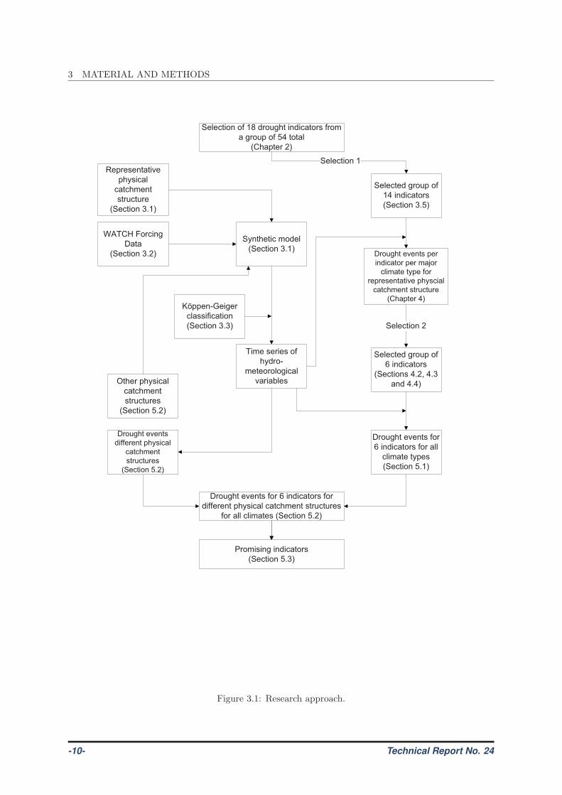
This chapter starts with a description of the data, models and techniques used for the assessment ofthe drought indicators on a global scale. Figure 3.1 gives a general overview of the methods used inthis research. A synthetic hydrological model is applied to generate time series of hydrometeorologicalvariables (Section 3.1). A global dataset is used as meteorological forcing data (Section 3.2). TheKopen-Geiger climate classification system will be applied to the global dataset with meteorologicalforcing data to find locations across the world with a specific climate type (Section 3.3). The thresholdapproach (Section 3.4) is used to classify the outcome from the selection of drought indicators, and todevelop drought indicators (i.e. droughts in precipitation, soil moisture, discharge). In the previouschapter a number of drought indicators have been described. A subset of potential useful indicators hasbeen identified and will be further described in Section 3.5. The performance of the selected droughtindicators will be calculated using the time series of hydrometeorological variables, either from the globalmeteorological dataset or the outcome from the synthetic model.
3.1 Synthetic model
The program NUT DAY that combines a soil water balance module and a simple conceptual hydrologicalmodule, was developed by Van Lanen et al. (1996) and is used in studies by Van Lanen & Tallaksen (2007;2008). The basic set-up is given in this section, as well as some specific details used in the calculationwith NUT DAY for this research. A full description of the latest model version is given by Van Lanenet al. (2010b). The model is used for the simulation of time series of soil moisture content, actualevapotranspiration, and recharge for different locations across the globe. The calculations of NUT DAYare done on a daily time step. A water balance equation is used in the calculation of NUT DAY, whichcan be written as:
S(t) = S(t− 1)−Qout(t) +Rch(t) (1)
SS(t) = SS(t− 1) + Pra(t) +Qsm(t)− ETa(t)−Rch(t) (2)
Ssn(t) = Ssn(t− 1) + Psn(t)−Qsm(t) (3)
where S, SS and Ssn are respectively the storage in the groundwater, the soil and the snowpack (inmm).Qout is the outflow from the groundwater and Rch is the recharge from the soil into the groundwater.Precipitation can either fall as rain (Pra) or snow (Psn). Snow that melts (Qsm) will enter the soil. Waterdisappears out of the soil through actual evapotranspiration (ETa). All fluxes are given in mm d−1, andcalculations are done for a daily time step.The hydrological module of NUT DAY is simulated like an linear reservoir. The storage in the reservoirdeterminates the rate of outflow (Qout). This outflow rate is defined by:
Qout(t) = Qout(t− 1) ∗ e−1/j +Rch(t) ∗ (1− e−1/j) (4)
which is the original de Zeeuw-Helling equation (Ritzema, 1994) and where j is descriped as:
j =π2 ∗ kD
µ ∗ L2(5)
where kD is the transmissivity (in m2d−1), µ is the storage coefficient and L is the distance betweenstreams (in m).
3.1.1 Precipitation
The synthetic model is fed by meteorological variables from a global dataset (Section 3.2). The precipita-tion is divided in snow and rain following the concept of the HBV snow routine (Seibert, 2005), which isincorporated into NUT DAY. For a given precipitation, HBV calculates, whether this precipitation willbe snow or rain based on the temperature. Snow accumulation is handled by the same snow routine ofHBV. The melt of snow starts when mean daily temperature is above a certain Threshold Temperature(TT ). The rate of snow melt depends on variable CFMAX. Other parameters are, snowfall correctionfactor SFCF , water holding capacity CWH, and the refreezing coefficient CFR. Default values for all
Technical Report No. 24 -9-
3 MATERIAL AND METHODS
������������ �������� ����������
��������������
����������
������������������������
��������
���������
���������
��������� ��
������� ������
���� �������
��������� ��
!���������������
�� �����������"��
�������������
����������������������
������������������
����������
������� ������
#�� �������
���������� �$� �
�� � ��
!��������������
#�� ������������
������������
��������� ��
!������������
��������������
���������
����������
��������� ��
%������������
���������
����������
��������� ��
&'(�)*������
!���
��������� ��
����������� ��
��������� ��
+,����-.�����
�������������
��������� ��
(����������
�� ��-
��������������
�����/���
����������
0���������� �������
��������� ��
!��������������#�� ���������
���������������������������������
���������������������� ��
Figure 3.1: Research approach.
-10- Technical Report No. 24
3 MATERIAL AND METHODS
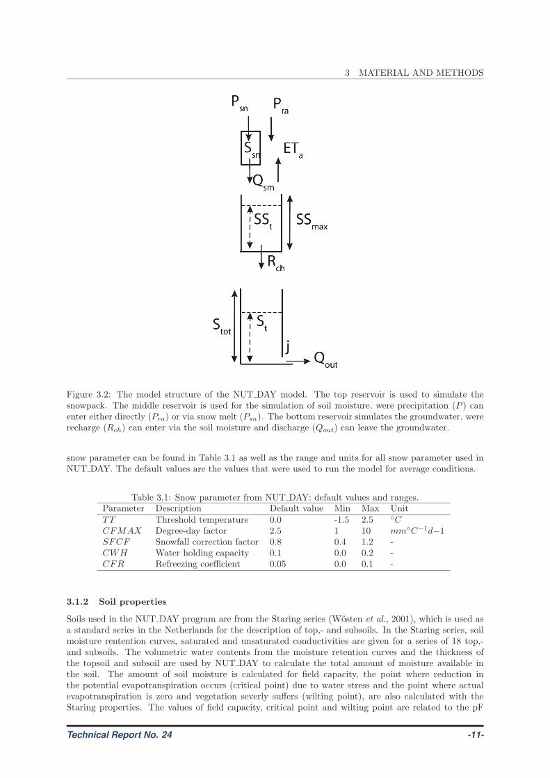
Figure 3.2: The model structure of the NUT DAY model. The top reservoir is used to simulate thesnowpack. The middle reservoir is used for the simulation of soil moisture, were precipitation (P ) canenter either directly (Pra) or via snow melt (Psn). The bottom reservoir simulates the groundwater, wererecharge (Rch) can enter via the soil moisture and discharge (Qout) can leave the groundwater.
snow parameter can be found in Table 3.1 as well as the range and units for all snow parameter used inNUT DAY. The default values are the values that were used to run the model for average conditions.
Table 3.1: Snow parameter from NUT DAY: default values and ranges.Parameter Description Default value Min Max UnitTT Threshold temperature 0.0 -1.5 2.5 ◦CCFMAX Degree-day factor 2.5 1 10 mm◦C−1d−1SFCF Snowfall correction factor 0.8 0.4 1.2 -CWH Water holding capacity 0.1 0.0 0.2 -CFR Refreezing coefficient 0.05 0.0 0.1 -
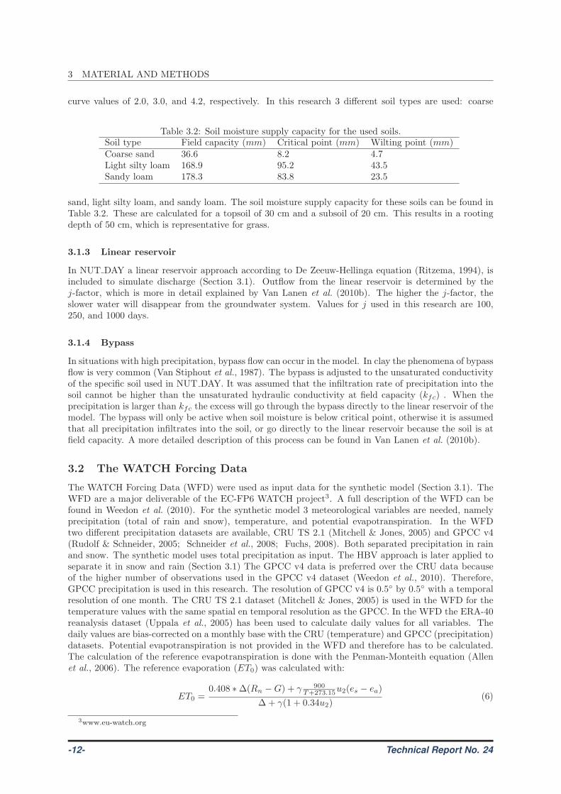
3.1.2 Soil properties
Soils used in the NUT DAY program are from the Staring series (Wosten et al., 2001), which is used asa standard series in the Netherlands for the description of top,- and subsoils. In the Staring series, soilmoisture rentention curves, saturated and unsaturated conductivities are given for a series of 18 top,-and subsoils. The volumetric water contents from the moisture retention curves and the thickness ofthe topsoil and subsoil are used by NUT DAY to calculate the total amount of moisture available inthe soil. The amount of soil moisture is calculated for field capacity, the point where reduction inthe potential evapotranspiration occurs (critical point) due to water stress and the point where actualevapotranspiration is zero and vegetation severly suffers (wilting point), are also calculated with theStaring properties. The values of field capacity, critical point and wilting point are related to the pF
Technical Report No. 24 -11-
3 MATERIAL AND METHODS
curve values of 2.0, 3.0, and 4.2, respectively. In this research 3 different soil types are used: coarse
Table 3.2: Soil moisture supply capacity for the used soils.Soil type Field capacity (mm) Critical point (mm) Wilting point (mm)Coarse sand 36.6 8.2 4.7Light silty loam 168.9 95.2 43.5Sandy loam 178.3 83.8 23.5
sand, light silty loam, and sandy loam. The soil moisture supply capacity for these soils can be found inTable 3.2. These are calculated for a topsoil of 30 cm and a subsoil of 20 cm. This results in a rootingdepth of 50 cm, which is representative for grass.
3.1.3 Linear reservoir
In NUT DAY a linear reservoir approach according to De Zeeuw-Hellinga equation (Ritzema, 1994), isincluded to simulate discharge (Section 3.1). Outflow from the linear reservoir is determined by thej-factor, which is more in detail explained by Van Lanen et al. (2010b). The higher the j-factor, theslower water will disappear from the groundwater system. Values for j used in this research are 100,250, and 1000 days.
3.1.4 Bypass
In situations with high precipitation, bypass flow can occur in the model. In clay the phenomena of bypassflow is very common (Van Stiphout et al., 1987). The bypass is adjusted to the unsaturated conductivityof the specific soil used in NUT DAY. It was assumed that the infiltration rate of precipitation into thesoil cannot be higher than the unsaturated hydraulic conductivity at field capacity (kfc) . When theprecipitation is larger than kfc the excess will go through the bypass directly to the linear reservoir of themodel. The bypass will only be active when soil moisture is below critical point, otherwise it is assumedthat all precipitation infiltrates into the soil, or go directly to the linear reservoir because the soil is atfield capacity. A more detailed description of this process can be found in Van Lanen et al. (2010b).
3.2 The WATCH Forcing Data
The WATCH Forcing Data (WFD) were used as input data for the synthetic model (Section 3.1). TheWFD are a major deliverable of the EC-FP6 WATCH project3. A full description of the WFD can befound in Weedon et al. (2010). For the synthetic model 3 meteorological variables are needed, namelyprecipitation (total of rain and snow), temperature, and potential evapotranspiration. In the WFDtwo different precipitation datasets are available, CRU TS 2.1 (Mitchell & Jones, 2005) and GPCC v4(Rudolf & Schneider, 2005; Schneider et al., 2008; Fuchs, 2008). Both separated precipitation in rainand snow. The synthetic model uses total precipitation as input. The HBV approach is later applied toseparate it in snow and rain (Section 3.1) The GPCC v4 data is preferred over the CRU data becauseof the higher number of observations used in the GPCC v4 dataset (Weedon et al., 2010). Therefore,GPCC precipitation is used in this research. The resolution of GPCC v4 is 0.5◦ by 0.5◦ with a temporalresolution of one month. The CRU TS 2.1 dataset (Mitchell & Jones, 2005) is used in the WFD for thetemperature values with the same spatial en temporal resolution as the GPCC. In the WFD the ERA-40reanalysis dataset (Uppala et al., 2005) has been used to calculate daily values for all variables. Thedaily values are bias-corrected on a monthly base with the CRU (temperature) and GPCC (precipitation)datasets. Potential evapotranspiration is not provided in the WFD and therefore has to be calculated.The calculation of the reference evapotranspiration is done with the Penman-Monteith equation (Allenet al., 2006). The reference evaporation (ET0) was calculated with:
ET0 =0.408 ∗∆(Rn −G) + γ 900
T+273.15u2(es − ea)
∆ + γ(1 + 0.34u2)(6)
3www.eu-watch.org
-12- Technical Report No. 24
3 MATERIAL AND METHODS
where ET0 is the reference evapotranspiration (mm d−1), Rn is net radiation at the surface (MJm−2
d−1), G is the soil heat flux density (MJ m−2 d−1), T is the mean daily temperature at 2 m height(◦C), u2 is the wind speed at 2 m height (m s−1), es is the saturation vapour pressure (kPa), es − eais the saturation vapour pressure deficit (kPa), ea is the actual vapour pressure (kPa), ∆ is the slopevapour pressure curve (kPa ◦C−1), and γ is the psychrometric constant (kPa ◦C−1). All variablesin the Penman-Monteith equation were either extracted from the WFD or calculated from variablesprovided through the WFD. The variables needed are the mean daily temperature (T ), and maximumand minimum temperature (Tmin and Tmax). Tmin and Tmax are used to calculated the saturated vapourpressure (es) with:
e0(T ) = 0.6108exp
[
17.27T
T + 237.3
]
(7)
es =e0(Tmax) + e0(Tmin)
2(8)
where e0(Tmax) and e0(Tmin) are first calculated using equation 7, before es is calculated. es can alsobe calculated using T , which results in a lower estimation of es that causes an underestimation of thereference evapotranspiration (Allen et al., 2006).The actual vapour pressure (ea) is calculated with q, the specific humidity (kg/kg) with:
ea =q ∗ P
ǫfrom Stull (2000) (9)
where ǫ is the ratio molecular weigth of water vapour/dry air which is equal to 0.62 and P the pressure inkPa. Net Radiation is calculated with short wave and net long wave radiation, both are provided throughin the WFD. The soil heat flux density G is assumed to be zero because it is very small compared to netsolar radiation Rn (Allen et al., 2006). It was assumed that the potential evapotranspiration equals thereference evapotranspiration (ET0), which is a fair approach for grass.
3.3 Koppen-Geiger classification
Performance of drought indicators will be investigated for different climate types of the world. TheKoppen-Geiger classification system has been chosen for this study, because it is still the most frequentlyused climate classification (Kottek et al., 2006). The application of this climate classification on theWATCH Forcing Data (WFD) enables the possibility to indentify locations in a particular climate type.The first Koppen classification was made by Koppen (1900) and updated by Geiger (1954; 1961). Basedon different vegetation types, Koppen distinguished five different major climate types and compiled aglobal map. The world is distributed in the equatorial zone (A), the arid zone (B), the warm temperaturezone (C), the snow zone (D), and the polar zone (E). The major climate types are subdivided intosubtypes based on precipitation regime and air temperature. This results in a classification systemof 31 different climate subtypes. The original maps of Koppen and Geiger were based on observations,which led to unequal spatial observation density. Peel et al. (2007) used the Global Historical ClimatologyNetwork version 2.0 (GHCN) dataset (Peterson & Vose, 1997) to make a revised Koppen-Geiger mapof the world. The availability of data in the GHCN is much higher than when Geiger made the updateof the Koppen-Geiger map of the world. A resolution of 0.1◦ by 0.1◦ was used to get a detailed globalmap. Since global datasets of precipitation and temperature have become available through interpolationof observations, digital versions of the original Koppen-Geiger maps are made by Kottek et al. (2006);Rubel & Kottek (2010). These maps have a 0.5◦ by 0.5◦ resolution and are available on a global scale.The difference between the study of Peel et al. (2007) and Kottek et al. (2006) is the interpolation ofdata. While, Kottek et al. (2006) relied on the interpolation of the CRU TS 2.1 (Mitchell & Jones, 2005)and GPCC (Rudolf & Schneider, 2005; Schneider et al., 2008; Fuchs, 2008) dataset. Peel et al. (2007)made their map based on his own interpolation from the GHCN dataset. The Koppen-Geiger climatetype can be determined for every location on the globe using one of these or both maps.In this study a global map of the Kopen-Geiger climate classification has been made with the WFD. Thiswas done to be able to compare location in the study based on climate type. To determine the climateof a certain location on the globe, minimally 30-year time series have to be used (World MeteorologicalOrganization, 2010). From these time series, monthly values for precipitation and temperature have
Technical Report No. 24 -13-
3 MATERIAL AND METHODS
to be calculated. For the identification of a climate type for a certain location, first the precipitationthreshold (Pth) in mm has to be calculated with:
Pth =2 ∗ Tann if > 66 % of precipitation occurs in winter2 ∗ Tann + 28 if > 66 % of precipitation occurs in summer2 ∗ Tann + 14 otherwise
(10)
where Tann is the mean annual temperature in◦C. The determination of B climates has to be done first,
because they are only based on the value of Pth, followed by the determination of the E climates becausethey only depend on temperature conditions. When first other major climate types are determined, a Bor a E climate can be wrongly classified because they match the requirements of other major climatesas well.After the major climate type is determined the subtype has to be found. This subtype will add asecond letter to the climate. This letter is based on the precipitation regime, except for E climateswhere this letter is based on temperature. For the B, C, and D climates a third letter is added basedon the temperature regime Eventually the procedure which in total results in 31 climate types. Thefull list of available subtypes and conditions can be found in Table 3.3. In this study, the Koppen-Geiger map of climate types across of the whole world was determined by using 44 years of WATCHForcing Data (WFD). The map from Kottek et al. (2006) was not suitable since the WFD has used adifferent precipitation dataset (Weedon et al., 2010). For a proper identification of the climate type anda consistent use of the true series of meteorological data for a selected location a new map had to bemade based on WFD. The map (Annex II) was used in this study to select the different locations andits associated climate.
3.4 The threshold method
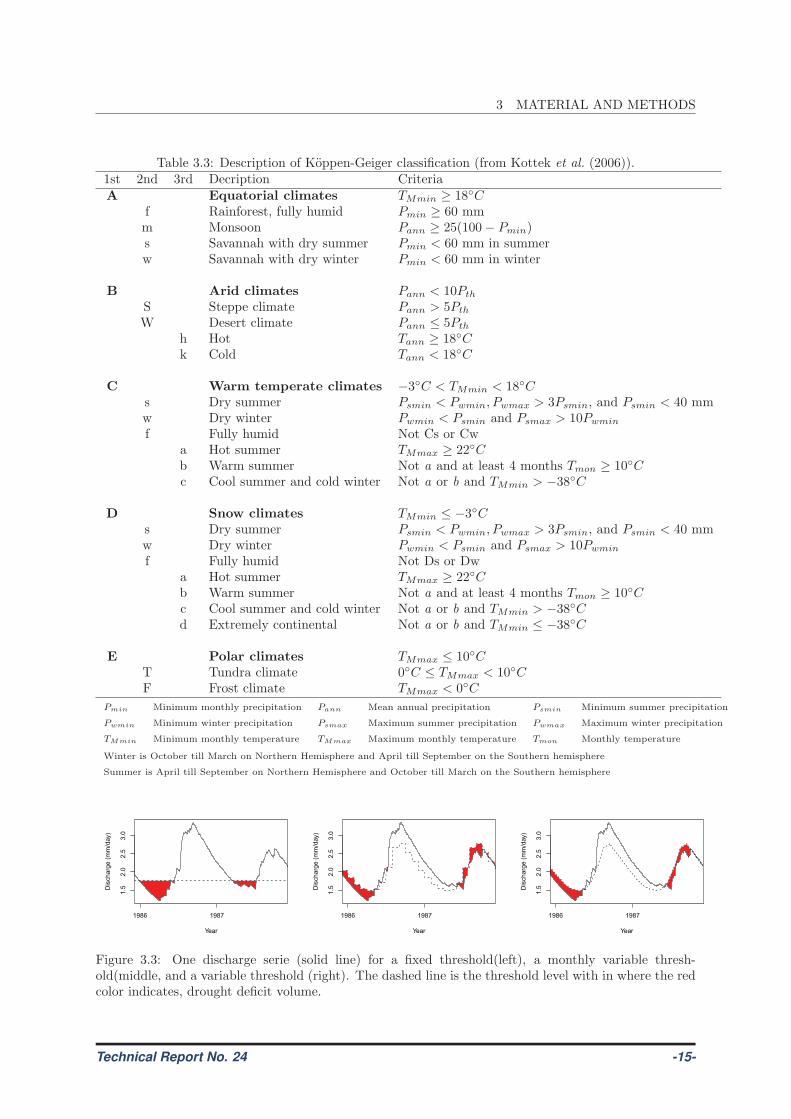
Time series of meteorological and hydrological variables are retrieved from the synthetic model (Sec-tion 3.1). These time series are used to calculate drought indicator performance and applied the thresh-old approach. The threshold method or truncation level method originates from the theory of runsdeveloped by Yevjevich (1967) and has been widely used since (Smakhtin, 2001). With the thresholdmethod, different drought characteristics can be determined (e.g duration and deficit volume) (Tallaksenet al., 1997; Hisdal et al., 2004; Fleig et al., 2006; Tallaksen et al., 2009). The method is basedon a threshold, when streamflow or another hydrometeorological variable is below this threshold it isconsidered a drought situation (Dracup et al., 1980; Hisdal et al., 2004). The threshold can be a fixedthreshold (FT) for the whole simulation periode, or a variable threshold (VT), which varies during theyear for every season, month or day (Fleig et al., 2006). The choice for a fixed or variable threshold isdependent on the purpose of the research. The threshold method can also be applied to precipitation,soil moisture content, and groundwater levels, but was originally developed for discharge. To calculatethe threshold, first all observed data are sorted from low to high. For drought determination the highestx percent is taken, as a normal or wet situation, everything below x percent will be a drought situation.The percentage that is chosen for x depends on the purpose and location of the study. In arid andsemi-arid conditions x can be as high as 50%, while normal values of x are between 70% and 95% (Hisdalet al., 2004).The threshold can be determined based on data from complete time series, which is done for a FT. Whena monthly VT is applied, observations for every month are combined and sorted separately, before thelowest x percent is determined for that month. When the moving average of the monthly VT is takenwith linear interpolation, a VT can be determined. This will result in a daily threshold derived from a30-day moving monthly threshold. The yearly FT, monthly VT, and VT are presented in Figure 3.3.For all types of threshold a drought is present if observed data are below the threshold,. The severity ofa drought can be determined by the calculation of the deficit volume. The higher this volume, the moresevere a drought will be. The deficit volume at time t (D(t)) can be calculated with:
D(t) =τ(t)−X(t) for X(t) < τ(t)0 for X(T ) ≥ τ(t) (11)
-14- Technical Report No. 24
3 MATERIAL AND METHODS
Table 3.3: Description of Koppen-Geiger classification (from Kottek et al. (2006)).1st 2nd 3rd Decription CriteriaA Equatorial climates TMmin ≥ 18◦C
f Rainforest, fully humid Pmin ≥ 60 mmm Monsoon Pann ≥ 25(100− Pmin)s Savannah with dry summer Pmin < 60 mm in summerw Savannah with dry winter Pmin < 60 mm in winter
B Arid climates Pann < 10Pth
S Steppe climate Pann > 5Pth
W Desert climate Pann ≤ 5Pth
h Hot Tann ≥ 18◦Ck Cold Tann < 18◦C
C Warm temperate climates −3◦C < TMmin < 18◦Cs Dry summer Psmin < Pwmin, Pwmax > 3Psmin, and Psmin < 40 mmw Dry winter Pwmin < Psmin and Psmax > 10Pwmin
f Fully humid Not Cs or Cwa Hot summer TMmax ≥ 22◦Cb Warm summer Not a and at least 4 months Tmon ≥ 10◦Cc Cool summer and cold winter Not a or b and TMmin > −38◦C
D Snow climates TMmin ≤ −3◦C
s Dry summer Psmin < Pwmin, Pwmax > 3Psmin, and Psmin < 40 mmw Dry winter Pwmin < Psmin and Psmax > 10Pwmin
f Fully humid Not Ds or Dwa Hot summer TMmax ≥ 22◦Cb Warm summer Not a and at least 4 months Tmon ≥ 10◦Cc Cool summer and cold winter Not a or b and TMmin > −38◦Cd Extremely continental Not a or b and TMmin ≤ −38
◦C
E Polar climates TMmax ≤ 10◦CT Tundra climate 0◦C ≤ TMmax < 10◦CF Frost climate TMmax < 0◦C
Pmin Minimum monthly precipitation Pann Mean annual precipitation Psmin Minimum summer precipitation
Pwmin Minimum winter precipitation Psmax Maximum summer precipitation Pwmax Maximum winter precipitation
TMmin Minimum monthly temperature TMmax Maximum monthly temperature Tmon Monthly temperature
Winter is October till March on Northern Hemisphere and April till September on the Southern hemisphere
Summer is April till September on Northern Hemisphere and October till March on the Southern hemisphere
Year
Dis
charg
e (
mm
/day)
1.5
2.0
2.5
3.0
1986 1987
Year
Dis
charg
e (
mm
/day)
1.5
2.0
2.5
3.0
1986 1987
Year
Dis
charg
e (
mm
/day)
1.5
2.0
2.5
3.0
1986 1987
Figure 3.3: One discharge serie (solid line) for a fixed threshold(left), a monthly variable thresh-old(middle, and a variable threshold (right). The dashed line is the threshold level with in where the redcolor indicates, drought deficit volume.
Technical Report No. 24 -15-
3 MATERIAL AND METHODS
Time
Dis
cha
rge
Low
Hig
h
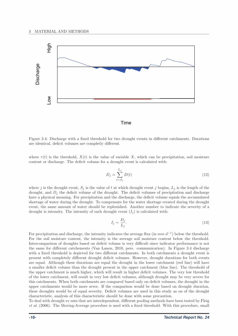
Figure 3.4: Discharge with a fixed threshold for two drought events in different catchments. Durationsare identical, deficit volumes are completly different.
where τ(t) is the threshold, X(t) is the value of variable X, which can be precipitation, soil moisturecontent or discharge. The deficit volume for a drought event is calculated with:
Dj =
Lj∑
t=Sj
D(t) (12)
where j is the drought event, Sj is the value of t at which drought event j begins, Lj is the length of thedrought, and Dj the deficit volume of the drought. The deficit volumes of precipitation and dischargehave a physical meaning. For precipitation and the discharge, the deficit volume equals the accumulatedshortage of water during the drought. To compensate for the water shortage created during the droughtevent, the same amount of water should be replenished. Another number to indicate the severity of adrought is intensity. The intensity of each drought event (Ij) is calculated with:
Ij =Dj
Lj. (13)
For precipitation and discharge, the intensity indicates the average flux (inmm d−1) below the threshold.For the soil moisture content, the intensity is the average soil moisture content below the threshold.Intercomparison of droughts based on deficit volume is very difficult since indicator performance is notthe same for different catchements (Van Lanen, 2010, pers. communication). In Figure 3.4 dischargewith a fixed threshold is depicted for two different catchments. In both catchments a drought event ispresent with completely different drought deficit volumes. However, drought durations for both eventsare equal. Although these durations are equal the drought in the lower catchment (red line) will havea smaller deficit volume than the drought present in the upper catchment (blue line). The threshold ofthe upper catchment is much higher, which will result in higher deficit volumes. The very low thresholdof the lower catchment, will result in very low deficit volumes, although drought may be very severe forthis catchments. When both catchments are compared based only on deficit volumes, the drought in theupper catchments would be more sever. If the comparison would be done based on drought duration,these droughts would be of equal severity. Deficit volumes are used in this study as on of the droughtcharacteristic, analysis of this characteristic should be done with some precaution.To deal with drought ev ents that are interdependent, different pooling methods have been tested by Fleiget al. (2006). The Moving-Average procedure is used with a fixed threshold. With this procedure, small
-16- Technical Report No. 24
3 MATERIAL AND METHODS
peaks above the threshold are removed by using the running average of the previous n-days (Tallaksenet al., 1997).
3.5 Selected drought indicators
In this section a more detailed description of selected indicators from Chapter 2 is given, includingequations to calculate the performance of each indicator and its classification (e.g. duration of droughts,severity of droughts, distinction of drought categories). The indicators were selected based on theirstrengths and weaknesses (Section 2) in combination with hydrological expert knowledge. Also twonew indicators are introduced, which likely will overcome some weak points of other methods. TheMoving Average precipitation (Section 3.5.1) uses a moving average to overcome difficulties in zerovalues of precipitation data. The standardized streamflow index (Section 3.5.3) uses a normalized gammadistribution to have a better estimation of low flows and is based on the same theory as the standardizedprecipitation index (Section 3.5.1). Fruthermore the SPI (Section 2.1) has been modified for use on adaily time step (Section 3.5.1).
3.5.1 Meteorological drought indicators
The Standardized Precipitation Index
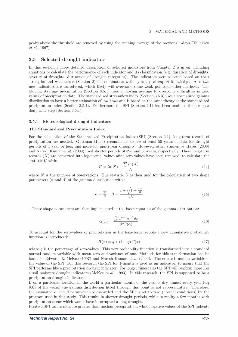
For the calculation of the Standardized Precipitation Index (SPI),(Section 2.1), long-term records ofprecipitation are needed. Guttman (1999) recommends to use at least 50 years of data for droughtperiods of 1 year or less, and more for multi-year droughts. However, other studies by Hayes (2006)and Naresh Kumar et al. (2009) used shorter periods of 39-, and 30-years, respectively. These long-termrecords (X) are converted into log-normal values after zero values have been removed, to calculate thestatistic U with:
U = ln(X)−
∑
ln(X)
N(14)
where N is the number of observations. The statistic U is then used for the calculation of two shapeparameters (α and β) of the gamma distribution with :
α = Xβ β =
1 +√
1 + 4U3
4U(15)
. These shape parameters are then implemented in the basic equation of the gamma distribution:
G(x) =
∫ x
0xa−1e
−xβ dx
βαΓ(α)(16)
To account for the zero-values of precipitation in the long-term records a new cumulative probabilityfunction is introduced:
H(x) = q + (1− q)G(x) (17)
where q is the percentage of zero-values. This new probability function is transformed into a standardnormal random variable with mean zero and variance of one. Methods for this transformation can befound in Edwards & McKee (1997) and Naresh Kumar et al. (2009). The created random variable isthe value of the SPI. For this research the SPI for 1-month is used as an indicator, to insure that theSPI performs like a precipitation drought indicator. For longer timescales the SPI will perform more likea soil moisture drought indicators (McKee et al., 1993). In this research, the SPI is supposed to be aprecipitation drought indicator.If on a particular location in the world a particular month of the year is dry almost every year (e.g90% of the years) the gamma distribution fitted through this point is not representative. Therefore,the estimated α and β parameter are discarded and the SPI is set to zero (normal conditions) by theprogram used in this study. This results in shorter drought periods, while in reality a few months withprecipitation occur which would have interrupted a long drought.Positive SPI values indicate greater than median precipitation, while negative values of the SPI indicate
Technical Report No. 24 -17-
3 MATERIAL AND METHODS
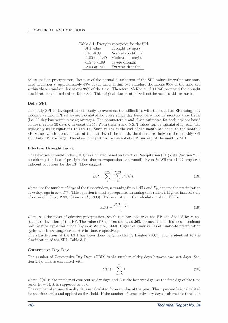
Table 3.4: Drought categories for the SPI.SPI value Drought category0 to -0.99 Normal conditions-1.00 to -1.49 Moderate drought-1.5 to -1.99 Severe drought-2.00 or less Extreme drought
below median precipitation. Because of the normal distribution of the SPI, values lie within one stan-dard deviation at approximately 68% of the time, within two standard deviations 95% of the time andwithin three standard deviations 98% of the time. Therefore, McKee et al. (1993) proposed the droughtclassification as described in Table 3.4. This original classification will not be used in this research.
Daily SPI
The daily SPI is developed in this study to overcome the difficulties with the standard SPI using onlymonthly values. SPI values are calculated for every single day based on a moving monthly time frame(i.e. 30-day backwards moving average). The parameters α and β are estimated for each day are basedon the previous 30 days with equation 15. With these α and β SPI values can be calculated for each dayseparately using equations 16 and 17. Since values at the end of the month are equal to the monthlySPI values which are calculated at the last day of the month, the differences between the monthly SPIand daily SPI are large. Therefore, it is justified to use a daily SPI instead of the monthly SPI.
Effective Drought Index
The Effective Drought Index (EDI) is calculated based on Effective Precipitation (EP) data (Section 2.1),considering the loss of precipitation due to evaporation and runoff. Byun & Wilhite (1999) exploreddifferent equations for the EP. They suggest:
EPi =n=1∑
i
[
(m=1∑
n
Pm)/n
]
(18)
where i as the number of days of the time window, n running from 1 till i and Pm denotes the precipitationofm days ago inmm d−1. This equation is most appropriate, assuming that runoff is highest immediatelyafter rainfall (Lee, 1998; Shim et al., 1998). The next step in the calculation of the EDI is:
EDI =EPi − µ
σ(19)
where µ is the mean of effective precipitation, which is subtracted from the EP and divided by σ, thestandard deviation of the EP. The value of i is often set at as 365, because the is this most dominantprecipitation cycle worldwide (Byun & Wilhite, 1999). Higher or lower values of i indicate precipitationcycles which are longer or shorter in time, respectively.The classification of the EDI has been done by Smakhtin & Hughes (2007) and is identical to theclassification of the SPI (Table 3.4).
Consecutive Dry Days
The number of Consecutive Dry Days (CDD) is the number of dry days between two wet days (Sec-tion 2.1). This is calculated with:
C(n) =
n∑
n−L
1 (20)
where C(n) is the number of consecutive dry days and L is the last wet day. At the first day of the timeseries (n = 0), L is supposed to be 0.The number of consecutive dry days is calculated for every day of the year. The x percentile is calculatedfor the time series and applied as threshold. If the number of consecutive dry days is above this threshold
-18- Technical Report No. 24
3 MATERIAL AND METHODS
Time
Pre
cip
itation (
mm
/day)
Daily precipitation
Moving Average Precipitation
05
10
15
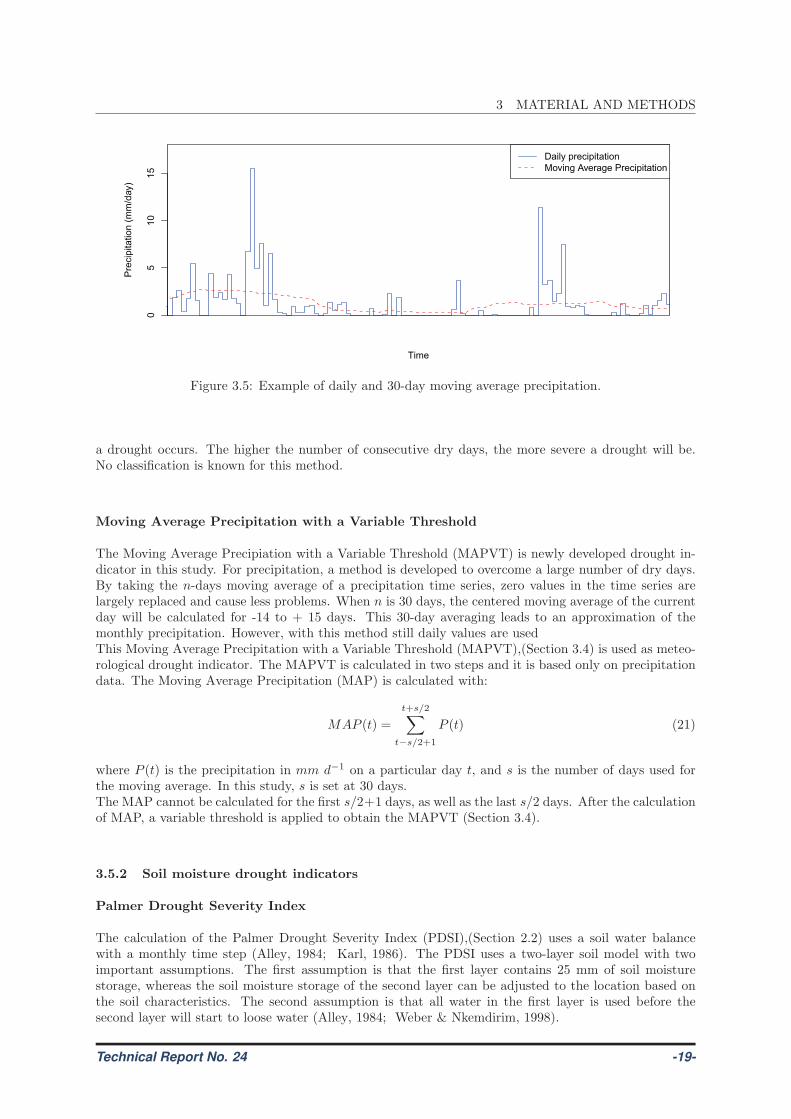
Figure 3.5: Example of daily and 30-day moving average precipitation.
a drought occurs. The higher the number of consecutive dry days, the more severe a drought will be.No classification is known for this method.
Moving Average Precipitation with a Variable Threshold
The Moving Average Precipiation with a Variable Threshold (MAPVT) is newly developed drought in-dicator in this study. For precipitation, a method is developed to overcome a large number of dry days.By taking the n-days moving average of a precipitation time series, zero values in the time series arelargely replaced and cause less problems. When n is 30 days, the centered moving average of the currentday will be calculated for -14 to + 15 days. This 30-day averaging leads to an approximation of themonthly precipitation. However, with this method still daily values are usedThis Moving Average Precipitation with a Variable Threshold (MAPVT),(Section 3.4) is used as meteo-rological drought indicator. The MAPVT is calculated in two steps and it is based only on precipitationdata. The Moving Average Precipitation (MAP) is calculated with:
MAP (t) =
t+s/2∑
t−s/2+1
P (t) (21)
where P (t) is the precipitation in mm d−1 on a particular day t, and s is the number of days used forthe moving average. In this study, s is set at 30 days.The MAP cannot be calculated for the first s/2+1 days, as well as the last s/2 days. After the calculationof MAP, a variable threshold is applied to obtain the MAPVT (Section 3.4).
3.5.2 Soil moisture drought indicators
Palmer Drought Severity Index
The calculation of the Palmer Drought Severity Index (PDSI),(Section 2.2) uses a soil water balancewith a monthly time step (Alley, 1984; Karl, 1986). The PDSI uses a two-layer soil model with twoimportant assumptions. The first assumption is that the first layer contains 25 mm of soil moisturestorage, whereas the soil moisture storage of the second layer can be adjusted to the location based onthe soil characteristics. The second assumption is that all water in the first layer is used before thesecond layer will start to loose water (Alley, 1984; Weber & Nkemdirim, 1998).
Technical Report No. 24 -19-
3 MATERIAL AND METHODS
Table 3.5: Drought categories for the PDSI.PDSI value Drought category1.49 to -1.49 Near normal-1.50 to -2.99 Mild to moderate drought-3.00 to -3.99 Severe drought-4.00 or less Extreme drought
The second step is the calculation of four monthly varying climate dependent coefficients:
αj = ETaj/ET0j βj = Rj/PRj
γj = ROj/PROj δj = Lj/PLj(22)
where j is the number of the specific month of the year. ETa, ET0, R, PR, RO, PRO, L and PLare the actual evapotranspiration, potential evapotranspiration, recharge, potential recharge, run-off,potential run-off, loss and potential loss, respectively, all in mm per month. Detailed information aboutthe calculation of the coefficients can be found in Alley (1984); Weber & Nkemdirim (1998); Cutoreet al. (2009). Next, the differences (d) between the actual precipitation and the Climatically AppropriateFor Existing Conditions (CAFEC), are calculated using:
di = Pi − (αj + βjPR+ γjPRO + δjPL) (23)
where Pi is precipitation in mm of the month i and (αj + βjPR+ γjPRO + δjPL) is the CAFEC inmm. The Z-index is calculated with:
Zi = d17.67K ′
i∑12
j=1 DjK ′
j
(24)
where Dj is the absolute value of all di values for each month i, K ′
i is:
K ′
i = 1.5log10
ET0i+Ri+ROi
Pi+Li
+ 2.8
Dj
+ 0.5 (25)
Finally the PDSI is calculated for each time step i with:
Xi = 0.897Xi−1 +
(
1
3
)
Zi (26)
with Xi is the PDSI value of the current month.Theoretically the values for the PDSI can vary between +10 and -10 (Dai et al., 2004). However, valuesnormally are between +4 and -4. Where +4 indicates extremely wet and -4 extremely dry conditions(Alley, 1984; Hayes, 1999). The dry part of the of the PDSI classification, can be found in Table 3.5.
Palmer Z-index
The Palmer Z-index (Section 2.2) is an intermediate term of the PDSI (equation 24) and represents themoisture anomaly of the current month. The Z-index reacts quickly to changes in soil moisture valueswithout a time delay as the PDSI (Karl, 1986).
Soil Moisture Deficit Index
The Soil Moisture Deficit Index (SMDI),(Section 2.2), needs a water balance model or observed soilmoisture data for the calculation of available soil moisture (Niemeijer, 2008). Long- term records ofsoil moisture for every week (j) of the year are required for the estimation of the median, minimumand maximum available soil moisture (Narasimhan & Srinivasan, 2005). Using the long-term median(MSWj), minimum (minSWj), and maximum (maxSWj) available soil moisture (SWi,j in mm), weekly
-20- Technical Report No. 24
3 MATERIAL AND METHODS
values (i) for the soil moisture deficit (SDi,j) are calculated using the following equations:
SDi,j =SWi,j −MSWj
MSWj −minSWj∗ 100 if SWi,j ≤MSWj
SDi,j =SWi,j −MSWj
maxSWj −MSWj∗ 100 if SWi,j > MSWj
(27)
where SDi,j is the soil water deficit (%) and SWi,j the weekly soil water availability in mm (Narasimhan& Srinivasan, 2005). SD values can vary from -100 to +100%, representing very dry or very wetconditions, respectively. The PDSI is used as a tool for comparison with the SMDI, therefore the SMDIis transformed in the same classification as the PDSI. The results is that the SMDI for any week (i) isgiven by:
SMDI1 =SD1
50Initial value
SMDIi = 0.5SMDIi−1 +SDi
50
(28)
Since the values of SD are dimensionless, comparison between different climate regions is possible as well(Narasimhan & Srinivasan, 2005).
Soil moisture content with a Variable Threshold
The Soil moisture content with a Variable Threshold (SVT)(Section 2.2) as a soil moisture droughtindicator. To calculate the SVT, a variable threshold (Section 3.4) is applied to the soil moisture contentof a particular day (Si).
Accumulated snow and soil moisture content
The Accumulated Snow and Soil Moisture content (ASSM) is newly developed in this study. The ASSMis calculated with:
ASSMi = ASi + SMi (29)
where i is the day, ASi the accumulated snow (in mm) and SMi the soil moisture content (in mm). Doidentify drought the threshold (Section 3.4) is applied in the same manner as done for the Soil moisturecontent with a Variable Threshold (Section 3.5.2).
3.5.3 Hydrological drought indicators
Groundwater Resource Index
The Groundwater Resource Indec (GRI) is based on four components of the water balance, namelyprecipiation, evapotranspiration, changes in soil moisture, and groundwater storage (Section 2.3). Forthe calculation of soil moisture storage and groundwater storage, a water balance model is needed. Fromthe model, only the groundwater retention is used as variable in the calculation of the GRI. The GRI isdefined as:
GRIi,j =Di,j − µD,j
σD,y(30)
where GRId,y is value of the GRI at day i in year j and D is the groundwater retention of the same day.µD,j and σD,j respectively are the mean and standard deviation of D for day d. For the calculation ofµD,j and σD,j , long term records of 30 year are recommended by Mendicino et al. (2008).Since there has been no classification for the GRI, the classification of the SPI is used. The sameclassification can be applied to both methods, because of the normal distribution of both the SPI andGRI.
Technical Report No. 24 -21-
3 MATERIAL AND METHODST
SD
I valu
es
J F M A M J J A S O N D
−2
−1
01
2
TS
DI valu
es
J F M A M J J A S O N D
−2
−1
01
2
Soil
mois
ture
sto
rage (
mm
)
J F M A M J J A S O N D
40
60
80
120
160
Soil
mois
ture
sto
rage (
mm
)
J F M A M J J A S O N D
60
80
100
140
Gro
undw
ate
r sto
rage (
mm
)
J F M A M J J A S O N D
0100
200
300
400
Gro
undw
ate
r sto
rage (
mm
)
J F M A M J J A S O N D
0200
400
600
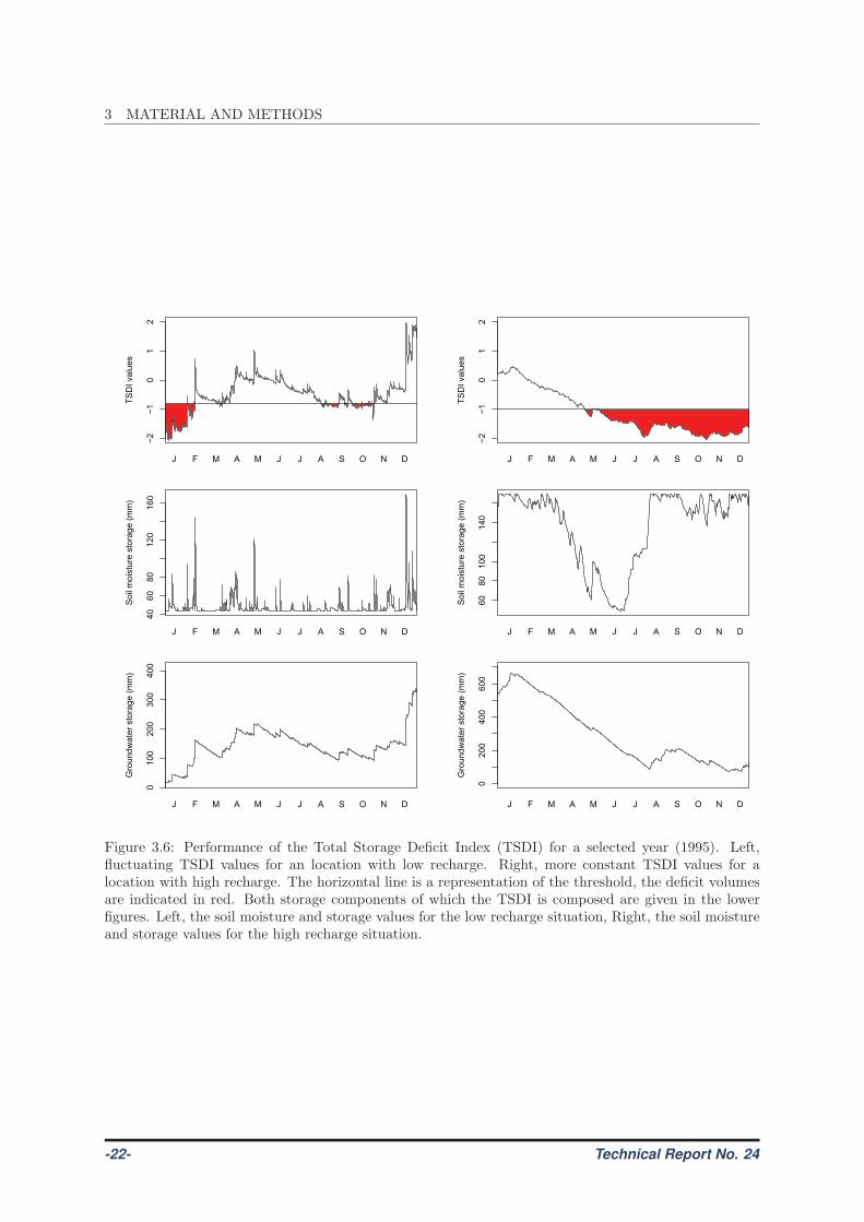
Figure 3.6: Performance of the Total Storage Deficit Index (TSDI) for a selected year (1995). Left,fluctuating TSDI values for an location with low recharge. Right, more constant TSDI values for alocation with high recharge. The horizontal line is a representation of the threshold, the deficit volumesare indicated in red. Both storage components of which the TSDI is composed are given in the lowerfigures. Left, the soil moisture and storage values for the low recharge situation, Right, the soil moistureand storage values for the high recharge situation.
-22- Technical Report No. 24
3 MATERIAL AND METHODS
Total Storage Deficit Index
The calculation of the Total Storage Deficit Index (TSDI),(Section 2.3) is based on the calculation ofthe SMDI (Yirdaw et al., 2008). The mean, maximum and minimum for every day (i) of the year (j)and the TSDI are calculated for a daily time step.First, the Total Storage Deficit (TSDi,j) is calculated with:
TSDi,j =TSAi,j −MTSAj
MaxTSAj −MinTSAj∗ 100 (31)
where TSA is the total storage (soil moisture and groundwater) at day i of year j. MTSAj , MaxTSAj ,and MinTSAj are the mean, maximum, and minimum of the TSA for that day of the year, respectively.The TSDI is calculated by standardizing the TSD values with:
TSDIi =TSDi − µ
σ(32)
where µ is the average value of TSD and σ is the standard deviation from the mean.The performance of the TSDI can be like a soil moisture or hydrological drought indicator. This is theresult of the combination of both the storage in the unsaturated zone and groundwater, in the calculationof the TSDI. In regions with high precipitation and recharge, the TSDI performs more like a hydrologicaldrought indicator. In these climates the amount of water in the unsaturated zone is small compared tothe amount of water in the saturated zone due. In regions with a low precipitation, the performance ofthe TSDI is more like a soil moisture drought indicator, because soil moisture is more important in theseclimates (Yirdaw et al., 2008). In Figure 3.6 this difference in performance is shown.
Discharge with a Variable Threshold
The Discharge with a Variable Threshold (QVT),(Section 2.3) is calculated in the same manner as theSoil Moisture content with a Variable Threshold (Section 3.5.2).
Standardized Streamflow Index
The Standardized Streamflow Index (SSI) is based on the same concept as the SPI. The SSI has beennewly developed in this study and uses a normalized gamma distribution for the daily discharge.The SSI is classified as a hydrological drought indicator. The only variable taken into account, is thedischarge.The indicator is developed to have better performance at locations where streamflow is zero for part ofthe year. When applying the threshold method, all the zero flows can cause difficulties (Simmers, 2003).With the use of the normalized gamma distribution these problems are solved.
3.5.4 Combined drought indicator
Aggregate Drought Index
The Aggregate Drought Index (ADI) is composed of six different variables (Section 2.4). The calculationof the ADI is complicated because of the six different variables. First, a matrix,
O(example) =
1.34 0.54 61 1.15 216 0.98...
......
......
...2.32 3.56 132 1.60 502 0.23
(33)
is composed with n by p dimensions, were n is the number of years of data and p the number ofvariables. For all the data in O, the means are subtracted and every element is divided by the standarddeviation, which results in matrix X. Correlations for each variable are calculated from matrix X to
Technical Report No. 24 -23-
3 MATERIAL AND METHODS
obtain correlation matrix R:
R(example) =
1 −0.68 0.4 0.32 0.38 −0.27...
......
......
...−0.27 0.38 −0.54 0.96 0.74 1
(34)
From R the eigenvector (e1) is calculated, which is associated with the first eigenvalue. X and e1 aremultiplied into vector Xe1 for which the standard deviation is calculated. The ADI is then calculatedwith:
ADI =Xe1µ
(35)
where Xe1 divided by µ, equals the standard deviation.
-24- Technical Report No. 24
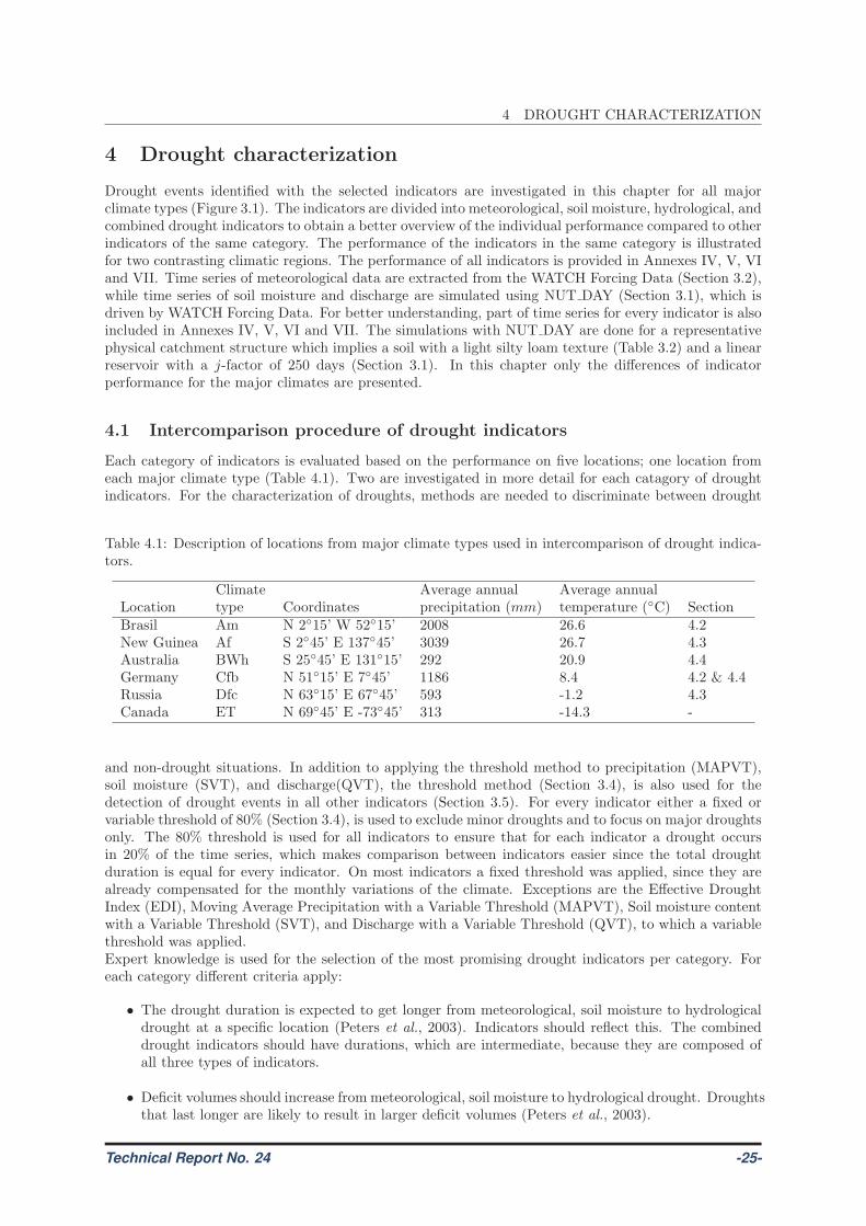
4 DROUGHT CHARACTERIZATION
4 Drought characterization
Drought events identified with the selected indicators are investigated in this chapter for all majorclimate types (Figure 3.1). The indicators are divided into meteorological, soil moisture, hydrological, andcombined drought indicators to obtain a better overview of the individual performance compared to otherindicators of the same category. The performance of the indicators in the same category is illustratedfor two contrasting climatic regions. The performance of all indicators is provided in Annexes IV, V, VIand VII. Time series of meteorological data are extracted from the WATCH Forcing Data (Section 3.2),while time series of soil moisture and discharge are simulated using NUT DAY (Section 3.1), which isdriven by WATCH Forcing Data. For better understanding, part of time series for every indicator is alsoincluded in Annexes IV, V, VI and VII. The simulations with NUT DAY are done for a representativephysical catchment structure which implies a soil with a light silty loam texture (Table 3.2) and a linearreservoir with a j-factor of 250 days (Section 3.1). In this chapter only the differences of indicatorperformance for the major climates are presented.
4.1 Intercomparison procedure of drought indicators
Each category of indicators is evaluated based on the performance on five locations; one location fromeach major climate type (Table 4.1). Two are investigated in more detail for each catagory of droughtindicators. For the characterization of droughts, methods are needed to discriminate between drought
Table 4.1: Description of locations from major climate types used in intercomparison of drought indica-tors.
Climate Average annual Average annualLocation type Coordinates precipitation (mm) temperature (◦C) SectionBrasil Am N 2◦15’ W 52◦15’ 2008 26.6 4.2New Guinea Af S 2◦45’ E 137◦45’ 3039 26.7 4.3Australia BWh S 25◦45’ E 131◦15’ 292 20.9 4.4Germany Cfb N 51◦15’ E 7◦45’ 1186 8.4 4.2 & 4.4Russia Dfc N 63◦15’ E 67◦45’ 593 -1.2 4.3Canada ET N 69◦45’ E -73◦45’ 313 -14.3 -
and non-drought situations. In addition to applying the threshold method to precipitation (MAPVT),soil moisture (SVT), and discharge(QVT), the threshold method (Section 3.4), is also used for thedetection of drought events in all other indicators (Section 3.5). For every indicator either a fixed orvariable threshold of 80% (Section 3.4), is used to exclude minor droughts and to focus on major droughtsonly. The 80% threshold is used for all indicators to ensure that for each indicator a drought occursin 20% of the time series, which makes comparison between indicators easier since the total droughtduration is equal for every indicator. On most indicators a fixed threshold was applied, since they arealready compensated for the monthly variations of the climate. Exceptions are the Effective DroughtIndex (EDI), Moving Average Precipitation with a Variable Threshold (MAPVT), Soil moisture contentwith a Variable Threshold (SVT), and Discharge with a Variable Threshold (QVT), to which a variablethreshold was applied.Expert knowledge is used for the selection of the most promising drought indicators per category. Foreach category different criteria apply:
• The drought duration is expected to get longer from meteorological, soil moisture to hydrologicaldrought at a specific location (Peters et al., 2003). Indicators should reflect this. The combineddrought indicators should have durations, which are intermediate, because they are composed ofall three types of indicators.
• Deficit volumes should increase from meteorological, soil moisture to hydrological drought. Droughtsthat last longer are likely to result in larger deficit volumes (Peters et al., 2003).
Technical Report No. 24 -25-
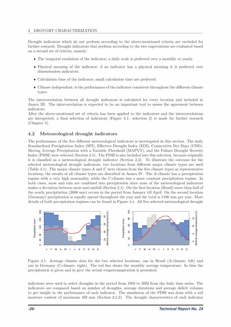
4 DROUGHT CHARACTERIZATION
Drought indicators which do not perform according to the above-mentioned criteria are excluded forfurther research. Drought indicators that perform according to the two expectations are evaluated basedon a second set of criteria, namely:
• The temporal resolution of the indicator; a daily scale is preferred over a monthly or yearly.
• Physical meaning of the indicator; if an indicator has a physical meaning it is preferred overdimensionless indicators.
• Calculation time of the indicator; small calculation time are preferred.
• Climate independent; is the performance of the indicator consistent throughout the different climatetypes.
The intercorrelation between all drought indicators is calculated for every location and included inAnnex III. The intercorrelation is expected to be an important tool to assess the agreement betweenindicators.After the above-mentioned set of criteria has been applied to the indicators and the intercorrelationsare interpreted, a final selection of indicators (Figure 3.1: selection 2) is made for further research(Chapter 5).
4.2 Meteorological drought indicators
The performance of the five different meteorological indicators is investigated in this section. The dailyStandardized Precipitation Index (SPI), Effective Drought Index (EDI), Consecutive Dry Days (CDD),Moving Average Precipitation with a Variable Threshold (MAPVT), and the Palmer Drought SeverityIndex (PDSI) were selected (Section 3.5). The PDSI is also included into this selection, because originallyit is classified as a meteorological drought indicator (Section 2.2). To illustrate the outcome for theselected meteorological drought indicators, two locations from different major climate types are used(Table 4.1). The major climate types A and C were chosen from the five climate types as representativelocations, the results of all climate types are described in Annex IV. The A-climate has a precipitationregime with a very high seasonality, while the C-climate has a more constant precipitation regime. Inboth cases, snow and rain are combined into precipitation since none of the meteorological indicatorsmakes a deviation between snow and rainfall (Section 2.1). On the first location (Brasil) more than half ofthe yearly precipitation (2008 mm) occurs in the period from January till April. On the second location(Germany) precipitation is equally spread throughout the year and the total is 1186 mm per year. Moredetails of both precipitation regimes can be found in Figure 4.1. All five selected meteorological drought
Month
Pre
cip
itation (
mm
)
040
80
140
200
260
J F M A M J J A S O N D
24
26
28
30
Month
ly a
vera
ge tem
pera
ture
(C
)
Month
Pre
cip
itation (
mm
)
020
40
60
80
100
J F M A M J J A S O N D
05
10
15
Month
ly a
vera
ge tem
pera
ture
(C
)
Figure 4.1: Average climate data for the two selected locations; one in Brazil (A-climate, left) andone in Germany (C-climate, right). The red line shows the monthly average temperature. In blue theprecipitation is given and in grey the actual evapotranspiration is presented.
indicators were used to select droughts in the period from 1958 to 2002 from the daily time series. Theindicators are compared based on number of droughts, average durations and average deficit volumesto get insight in the performance of each indicator. The simulation of the PDSI was done with a soilmoisture content of maximum 169 mm (Section 3.5.2). The drought characteristics of each indicator
-26- Technical Report No. 24
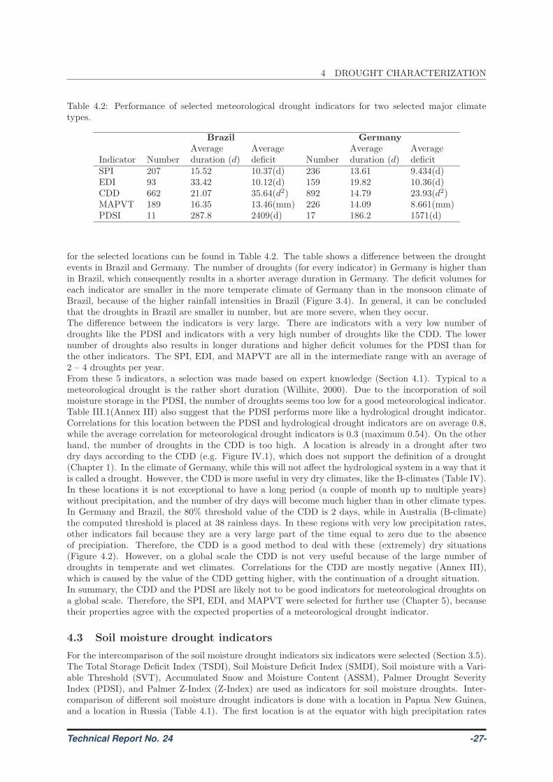
4 DROUGHT CHARACTERIZATION
Table 4.2: Performance of selected meteorological drought indicators for two selected major climatetypes.
Brazil Germany
Average Average Average AverageIndicator Number duration (d) deficit Number duration (d) deficitSPI 207 15.52 10.37(d) 236 13.61 9.434(d)EDI 93 33.42 10.12(d) 159 19.82 10.36(d)CDD 662 21.07 35.64(d2) 892 14.79 23.93(d2)MAPVT 189 16.35 13.46(mm) 226 14.09 8.661(mm)PDSI 11 287.8 2409(d) 17 186.2 1571(d)
for the selected locations can be found in Table 4.2. The table shows a difference between the droughtevents in Brazil and Germany. The number of droughts (for every indicator) in Germany is higher thanin Brazil, which consequently results in a shorter average duration in Germany. The deficit volumes foreach indicator are smaller in the more temperate climate of Germany than in the monsoon climate ofBrazil, because of the higher rainfall intensities in Brazil (Figure 3.4). In general, it can be concludedthat the droughts in Brazil are smaller in number, but are more severe, when they occur.The difference between the indicators is very large. There are indicators with a very low number ofdroughts like the PDSI and indicators with a very high number of droughts like the CDD. The lowernumber of droughts also results in longer durations and higher deficit volumes for the PDSI than forthe other indicators. The SPI, EDI, and MAPVT are all in the intermediate range with an average of2 – 4 droughts per year.From these 5 indicators, a selection was made based on expert knowledge (Section 4.1). Typical to ameteorological drought is the rather short duration (Wilhite, 2000). Due to the incorporation of soilmoisture storage in the PDSI, the number of droughts seems too low for a good meteorological indicator.Table III.1(Annex III) also suggest that the PDSI performs more like a hydrological drought indicator.Correlations for this location between the PDSI and hydrological drought indicators are on average 0.8,while the average correlation for meteorological drought indicators is 0.3 (maximum 0.54). On the otherhand, the number of droughts in the CDD is too high. A location is already in a drought after twodry days according to the CDD (e.g. Figure IV.1), which does not support the definition of a drought(Chapter 1). In the climate of Germany, while this will not affect the hydrological system in a way that itis called a drought. However, the CDD is more useful in very dry climates, like the B-climates (Table IV).In these locations it is not exceptional to have a long period (a couple of month up to multiple years)without precipitation, and the number of dry days will become much higher than in other climate types.In Germany and Brazil, the 80% threshold value of the CDD is 2 days, while in Australia (B-climate)the computed threshold is placed at 38 rainless days. In these regions with very low precipitation rates,other indicators fail because they are a very large part of the time equal to zero due to the absenceof precipiation. Therefore, the CDD is a good method to deal with these (extremely) dry situations(Figure 4.2). However, on a global scale the CDD is not very useful because of the large number ofdroughts in temperate and wet climates. Correlations for the CDD are mostly negative (Annex III),which is caused by the value of the CDD getting higher, with the continuation of a drought situation.In summary, the CDD and the PDSI are likely not to be good indicators for meteorological droughts ona global scale. Therefore, the SPI, EDI, and MAPVT were selected for further use (Chapter 5), becausetheir properties agree with the expected properties of a meteorological drought indicator.
4.3 Soil moisture drought indicators
For the intercomparison of the soil moisture drought indicators six indicators were selected (Section 3.5).The Total Storage Deficit Index (TSDI), Soil Moisture Deficit Index (SMDI), Soil moisture with a Vari-able Threshold (SVT), Accumulated Snow and Moisture Content (ASSM), Palmer Drought SeverityIndex (PDSI), and Palmer Z-Index (Z-Index) are used as indicators for soil moisture droughts. Inter-comparison of different soil moisture drought indicators is done with a location in Papua New Guinea,and a location in Russia (Table 4.1). The first location is at the equator with high precipitation rates
Technical Report No. 24 -27-
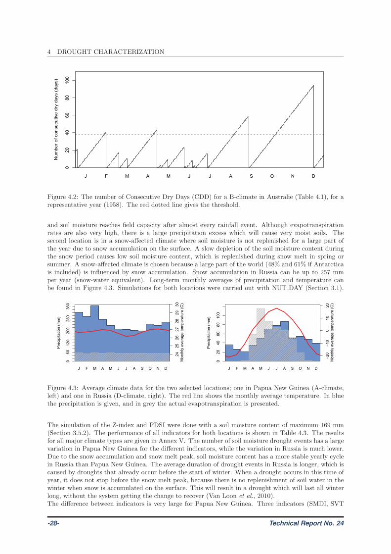
4 DROUGHT CHARACTERIZATIONN
um
ber
of consecutive d
ry d
ays (
days)
J F M A M J J A S O N D
020
40
60
80
100
Figure 4.2: The number of Consecutive Dry Days (CDD) for a B-climate in Australie (Table 4.1), for arepresentative year (1958). The red dotted line gives the threshold.
and soil moisture reaches field capacity after almost every rainfall event. Although evapotranspirationrates are also very high, there is a large precipitation excess which will cause very moist soils. Thesecond location is in a snow-affected climate where soil moisture is not replenished for a large part ofthe year due to snow accumulation on the surface. A slow depletion of the soil moisture content duringthe snow period causes low soil moisture content, which is replenished during snow melt in spring orsummer. A snow-affected climate is chosen because a large part of the world (48% and 61% if Antarcticais included) is influenced by snow accumulation. Snow accumulation in Russia can be up to 257 mmper year (snow-water equivalent). Long-term monthly averages of precipitation and temperature canbe found in Figure 4.3. Simulations for both locations were carried out with NUT DAY (Section 3.1).
Month
Pre
cip
itation (
mm
)
060
120
200
280
360
J F M A M J J A S O N D
24
25
26
27
28
29
30
Month
ly a
vera
ge tem
pera
ture
(C
)
Month
Pre
cip
itation (
mm
)
020
40
60
80
100
J F M A M J J A S O N D
−20
−10
010
20
Month
ly a
vera
ge tem
pera
ture
(C
)
Figure 4.3: Average climate data for the two selected locations; one in Papua New Guinea (A-climate,left) and one in Russia (D-climate, right). The red line shows the monthly average temperature. In bluethe precipitation is given, and in grey the actual evapotranspiration is presented.
The simulation of the Z-index and PDSI were done with a soil moisture content of maximum 169 mm(Section 3.5.2). The performance of all indicators for both locations is shown in Table 4.3. The resultsfor all major climate types are given in Annex V. The number of soil moisture drought events has a largevariation in Papua New Guinea for the different indicators, while the variation in Russia is much lower.Due to the snow accumulation and snow melt peak, soil moisture content has a more stable yearly cyclein Russia than Papua New Guinea. The average duration of drought events in Russia is longer, which iscaused by droughts that already occur before the start of winter. When a drought occurs in this time ofyear, it does not stop before the snow melt peak, because there is no replenishment of soil water in thewinter when snow is accumulated on the surface. This will result in a drought which will last all winterlong, without the system getting the change to recover (Van Loon et al., 2010).The difference between indicators is very large for Papua New Guinea. Three indicators (SMDI, SVT
-28- Technical Report No. 24
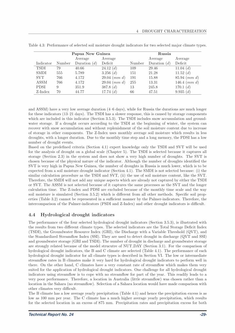
4 DROUGHT CHARACTERIZATION
Table 4.3: Performance of selected soil moisture drought indicators for two selected major climate types.
Papua New Guinea Russia
Average Average Average AverageIndicator Number Duration (d) Deficit Number Duration (d) DeficitTSDI 79 40.66 24.12 (d) 109 29.46 11.04 (d)SMDI 555 5.789 3.256 (d) 151 21.28 11.52 (d)SVT 766 4.172 29.04 (mm d) 191 15.88 85.94 (mm d)ASSM 766 4.172 29.04 (mm d) 255 13.31 146.4 (mm d)PDSI 9 351.9 387.8 (d) 13 245.8 170.1 (d)Z-Index 70 44.77 17.74 (d) 66 47.51 9.935 (d)
and ASSM) have a very low average duration (4–6 days), while for Russia the durations are much longerfor these indicators (13–21 days). The TSDI has a slower response, this is caused by storage componentswhich are included in this indicator (Section 3.5.3). The TSDI includes snow accumulation and ground-water storage. If a drought occurs according to the TSDI at the beginning of winter, the system canrecover with snow accumulation and without replenishment of the soil moisture content due to increaseof storage in other components. The Z-Index uses monthly average soil moisture which results in lessdroughts, with a longer duration. Due to the monthly time step and a long memory, the PDSI has a lownumber of drought events.Based on the predefined criteria (Section 4.1) expert knowledge only the TSDI and SVT will be usedfor the analysis of drought on a global scale (Chapter 5). The TSDI is selected because it captures allstorage (Section 2.3) in the system and does not show a very high number of droughts. The SVT ischosen because of the physical nature of the indicator. Although the number of droughts identified theSVT is very high in Papua New Guinea, the number of droughts in Russia is much lower, which is to beexpected from a soil moisture drought indicator (Section 4.1). The SMDI is not selected because: (i) thesimilar calculation procedure as the TSDI and SVT, (ii) the use of soil moisture content, like the SVT.Therefore, the SMDI will not add any unique aspects which are already not captured by either the TSDIor SVT. The ASSM is not selected because of it captures the same processes as the SVT and the longercalculation time. The Z-index and PDSI are excluded because of the monthly time scale and the waysoil moisture is simulated (Section 3.5.2) which is different from all other methods. Specific soil prop-erties (Table 3.2) cannot be represented in a sufficient manner by the Palmer-indicators. Therefore, theintercomparison of the Palmer-indicators (PSDI and Z-Index) and other drought indicators is difficult.
4.4 Hydrological drought indicators
The performance of the four selected hydrological drought indicators (Section 3.5.3), is illustrated withthe results from two different climate types. The selected indicators are the Total Storage Deficit Index(TSDI), the Groundwater Resource Index (GRI), the Discharge with a Variable Threshold (QVT), andthe Standardized Streamflow Index (SSI). They are used to detect drought in discharge (QVT and SSI)and groundwater storage (GRI and TSDI). The number of drought in discharge and groundwater storageare strongly related because of the model strucutre of NUT DAY (Section 3.1). For the comparison ofhydrological drought indicators, the B and C climate are selected (Table 4.1). The performance of eachhydrological drought indicator for all climate types is described in Section VI. The low or intermediatestreamflow rates in B climates make it very hard for hydrological drought indicators to perform well inthere. On the other hand, C climates have a very constant rate of streamflow which makes them verysuited for the application of hydrological drought indicators. One challenge for all hydrological droughtindicators using streamflow is to cope with no streamflow for part of the year. This readily leads to avery poor performance. Therefore, a location in Australia (little streamflow) was chosen rather than alocation in the Sahara (no streamflow). Selection of a Sahara location would have made comparison withother climates very difficult.The B climate has a low average yearly precipitation (Table 4.1) and hence the precipitation excess is aslow as 100 mm per year. The C climate has a much higher average yearly precipitation, which resultsfor the selected location in an excess of 875 mm. Precipitation rates and precipitation excess for both
Technical Report No. 24 -29-
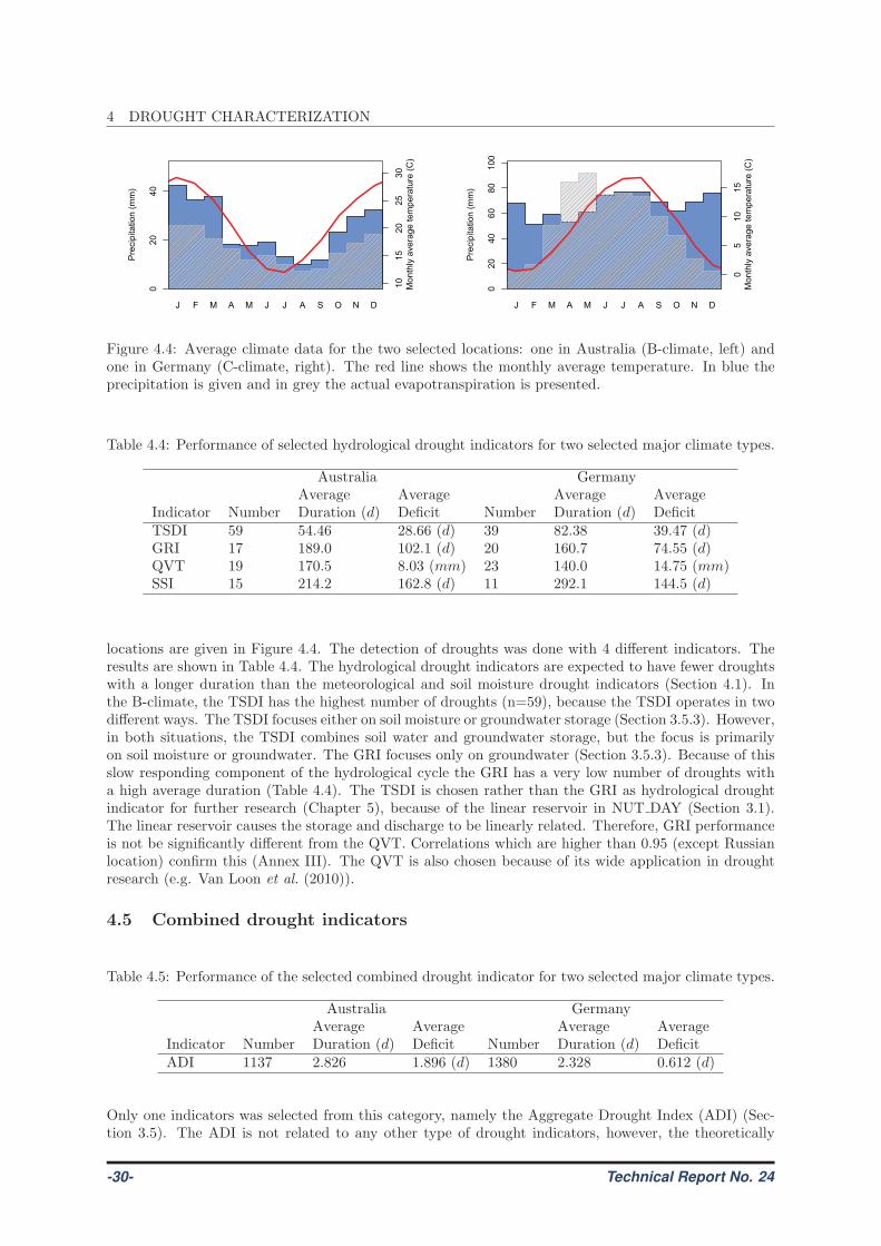
4 DROUGHT CHARACTERIZATION
Month
Pre
cip
itation (
mm
)
020
40
J F M A M J J A S O N D
10
15
20
25
30
Month
ly a
vera
ge tem
pera
ture
(C
)
Month
Pre
cip
itation (
mm
)
020
40
60
80
100
J F M A M J J A S O N D
05
10
15
Month
ly a
vera
ge tem
pera
ture
(C
)
Figure 4.4: Average climate data for the two selected locations: one in Australia (B-climate, left) andone in Germany (C-climate, right). The red line shows the monthly average temperature. In blue theprecipitation is given and in grey the actual evapotranspiration is presented.
Table 4.4: Performance of selected hydrological drought indicators for two selected major climate types.
Australia GermanyAverage Average Average Average
Indicator Number Duration (d) Deficit Number Duration (d) DeficitTSDI 59 54.46 28.66 (d) 39 82.38 39.47 (d)GRI 17 189.0 102.1 (d) 20 160.7 74.55 (d)QVT 19 170.5 8.03 (mm) 23 140.0 14.75 (mm)SSI 15 214.2 162.8 (d) 11 292.1 144.5 (d)
locations are given in Figure 4.4. The detection of droughts was done with 4 different indicators. Theresults are shown in Table 4.4. The hydrological drought indicators are expected to have fewer droughtswith a longer duration than the meteorological and soil moisture drought indicators (Section 4.1). Inthe B-climate, the TSDI has the highest number of droughts (n=59), because the TSDI operates in twodifferent ways. The TSDI focuses either on soil moisture or groundwater storage (Section 3.5.3). However,in both situations, the TSDI combines soil water and groundwater storage, but the focus is primarilyon soil moisture or groundwater. The GRI focuses only on groundwater (Section 3.5.3). Because of thisslow responding component of the hydrological cycle the GRI has a very low number of droughts witha high average duration (Table 4.4). The TSDI is chosen rather than the GRI as hydrological droughtindicator for further research (Chapter 5), because of the linear reservoir in NUT DAY (Section 3.1).The linear reservoir causes the storage and discharge to be linearly related. Therefore, GRI performanceis not be significantly different from the QVT. Correlations which are higher than 0.95 (except Russianlocation) confirm this (Annex III). The QVT is also chosen because of its wide application in droughtresearch (e.g. Van Loon et al. (2010)).
4.5 Combined drought indicators
Table 4.5: Performance of the selected combined drought indicator for two selected major climate types.
Australia GermanyAverage Average Average Average
Indicator Number Duration (d) Deficit Number Duration (d) DeficitADI 1137 2.826 1.896 (d) 1380 2.328 0.612 (d)
Only one indicators was selected from this category, namely the Aggregate Drought Index (ADI) (Sec-tion 3.5). The ADI is not related to any other type of drought indicators, however, the theoretically
-30- Technical Report No. 24
4 DROUGHT CHARACTERIZATION
it resembles hydrological drought indicators most. Therefore, as for the hydrological indicators (Sec-tion 3.5.3) the B and C climate are used to illustrate the results of the ADI. The details of both locationsare described in Figure 4.4. The climatic results for the all climate types are given in Section VII. Theresults for climate types B and C are shown in Table 4.5. The ADI has the highest number of droughts,compared to all previous drought indicators. Even the meteorological drought indicators have a lowernumber of droughts (Table 4.5). Meteorological drought indicators are expected to have a higher numberthan a combined indicator, which is assumed to have intermediate number of droughts (Section 4.1).This number is too high for wider analysis on a global scale (Chapter 5). The ADI shows no correlationwith any of the previously selection indicators (Annex III). Therefore, the ADI is not selected for furtherresearch.
Technical Report No. 24 -31-

4 DROUGHT CHARACTERIZATION
-32- Technical Report No. 24
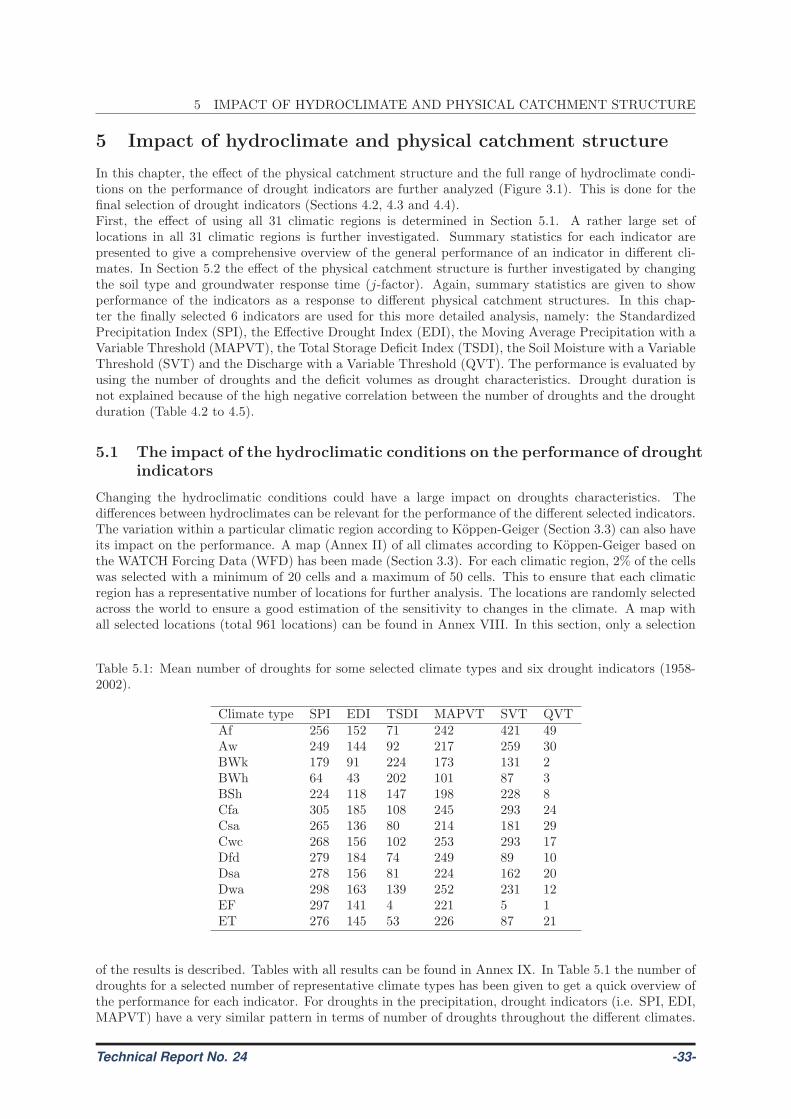
5 IMPACT OF HYDROCLIMATE AND PHYSICAL CATCHMENT STRUCTURE
5 Impact of hydroclimate and physical catchment structure
In this chapter, the effect of the physical catchment structure and the full range of hydroclimate condi-tions on the performance of drought indicators are further analyzed (Figure 3.1). This is done for thefinal selection of drought indicators (Sections 4.2, 4.3 and 4.4).First, the effect of using all 31 climatic regions is determined in Section 5.1. A rather large set oflocations in all 31 climatic regions is further investigated. Summary statistics for each indicator arepresented to give a comprehensive overview of the general performance of an indicator in different cli-mates. In Section 5.2 the effect of the physical catchment structure is further investigated by changingthe soil type and groundwater response time (j-factor). Again, summary statistics are given to showperformance of the indicators as a response to different physical catchment structures. In this chap-ter the finally selected 6 indicators are used for this more detailed analysis, namely: the StandardizedPrecipitation Index (SPI), the Effective Drought Index (EDI), the Moving Average Precipitation with aVariable Threshold (MAPVT), the Total Storage Deficit Index (TSDI), the Soil Moisture with a VariableThreshold (SVT) and the Discharge with a Variable Threshold (QVT). The performance is evaluated byusing the number of droughts and the deficit volumes as drought characteristics. Drought duration isnot explained because of the high negative correlation between the number of droughts and the droughtduration (Table 4.2 to 4.5).
5.1 The impact of the hydroclimatic conditions on the performance of droughtindicators
Changing the hydroclimatic conditions could have a large impact on droughts characteristics. Thedifferences between hydroclimates can be relevant for the performance of the different selected indicators.The variation within a particular climatic region according to Koppen-Geiger (Section 3.3) can also haveits impact on the performance. A map (Annex II) of all climates according to Koppen-Geiger based onthe WATCH Forcing Data (WFD) has been made (Section 3.3). For each climatic region, 2% of the cellswas selected with a minimum of 20 cells and a maximum of 50 cells. This to ensure that each climaticregion has a representative number of locations for further analysis. The locations are randomly selectedacross the world to ensure a good estimation of the sensitivity to changes in the climate. A map withall selected locations (total 961 locations) can be found in Annex VIII. In this section, only a selection
Table 5.1: Mean number of droughts for some selected climate types and six drought indicators (1958-2002).
Climate type SPI EDI TSDI MAPVT SVT QVTAf 256 152 71 242 421 49Aw 249 144 92 217 259 30BWk 179 91 224 173 131 2BWh 64 43 202 101 87 3BSh 224 118 147 198 228 8Cfa 305 185 108 245 293 24Csa 265 136 80 214 181 29Cwc 268 156 102 253 293 17Dfd 279 184 74 249 89 10Dsa 278 156 81 224 162 20Dwa 298 163 139 252 231 12EF 297 141 4 221 5 1ET 276 145 53 226 87 21
of the results is described. Tables with all results can be found in Annex IX. In Table 5.1 the number ofdroughts for a selected number of representative climate types has been given to get a quick overview ofthe performance for each indicator. For droughts in the precipitation, drought indicators (i.e. SPI, EDI,MAPVT) have a very similar pattern in terms of number of droughts throughout the different climates.
Technical Report No. 24 -33-
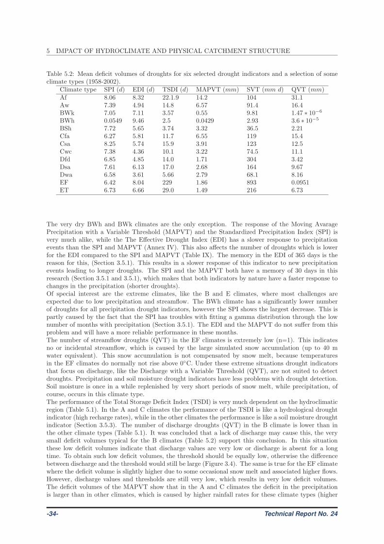
5 IMPACT OF HYDROCLIMATE AND PHYSICAL CATCHMENT STRUCTURE
Table 5.2: Mean deficit volumes of droughts for six selected drought indicators and a selection of someclimate types (1958-2002).
Climate type SPI (d) EDI (d) TSDI (d) MAPVT (mm) SVT (mm d) QVT (mm)Af 8.06 8.32 22.1.9 14.2 104 31.1Aw 7.39 4.94 14.8 6.57 91.4 16.4BWk 7.05 7.11 3.57 0.55 9.81 1.47 ∗ 10−6
BWh 0.0549 9.46 2.5 0.0429 2.93 3.6 ∗ 10−5
BSh 7.72 5.65 3.74 3.32 36.5 2.21Cfa 6.27 5.81 11.7 6.55 119 15.4Csa 8.25 5.74 15.9 3.91 123 12.5Cwc 7.38 4.36 10.1 3.22 74.5 11.1Dfd 6.85 4.85 14.0 1.71 304 3.42Dsa 7.61 6.13 17.0 2.68 164 9.67Dwa 6.58 3.61 5.66 2.79 68.1 8.16EF 6.42 8.04 229 1.86 893 0.0951ET 6.73 6.66 29.0 1.49 216 6.73
The very dry BWh and BWk climates are the only exception. The response of the Moving AvaragePrecipitation with a Variable Threshold (MAPVT) and the Standardized Precipitation Index (SPI) isvery much alike, while the The Effective Drought Index (EDI) has a slower response to precipitationevents than the SPI and MAPVT (Annex IV). This also affects the number of droughts which is lowerfor the EDI compared to the SPI and MAPVT (Table IX). The memory in the EDI of 365 days is thereason for this, (Section 3.5.1). This results in a slower response of this indicator to new precipitationevents leading to longer droughts. The SPI and the MAPVT both have a memory of 30 days in thisresearch (Section 3.5.1 and 3.5.1), which makes that both indicators by nature have a faster response tochanges in the precipitation (shorter droughts).Of special interest are the extreme climates, like the B and E climates, where most challenges areexpected due to low precipitation and streamflow. The BWh climate has a significantly lower numberof droughts for all precipitation drought indicators, however the SPI shows the largest decrease. This ispartly caused by the fact that the SPI has troubles with fitting a gamma distribution through the lownumber of months with precipitation (Section 3.5.1). The EDI and the MAPVT do not suffer from thisproblem and will have a more reliable performance in these months.The number of streamflow droughts (QVT) in the EF climates is extremely low (n=1). This indicatesno or incidental streamflow, which is caused by the large simulated snow accumulation (up to 40 mwater equivalent). This snow accumulation is not compensated by snow melt, because temperaturesin the EF climates do normally not rise above 0◦C. Under these extreme situations drought indicatorsthat focus on discharge, like the Discharge with a Variable Threshold (QVT), are not suited to detectdroughts. Precipitation and soil moisture drought indicators have less problems with drought detection.Soil moisture is once in a while replenished by very short periods of snow melt, while precipitation, ofcourse, occurs in this climate type.The performance of the Total Storage Deficit Index (TSDI) is very much dependent on the hydroclimaticregion (Table 5.1). In the A and C climates the performance of the TSDI is like a hydrological droughtindicator (high recharge rates), while in the other climates the performance is like a soil moisture droughtindicator (Section 3.5.3). The number of discharge droughts (QVT) in the B climate is lower than inthe other climate types (Table 5.1). It was concluded that a lack of discharge may cause this, the verysmall deficit volumes typical for the B climates (Table 5.2) support this conclusion. In this situationthese low deficit volumes indicate that discharge values are very low or discharge is absent for a longtime. To obtain such low deficit volumes, the threshold should be equally low, otherwise the differencebetween discharge and the threshold would still be large (Figure 3.4). The same is true for the EF climatewhere the deficit volume is slightly higher due to some occasional snow melt and associated higher flows.However, discharge values and thresholds are still very low, which results in very low deficit volumes.The deficit volumes of the MAPVT show that in the A and C climates the deficit in the precipitationis larger than in other climates, which is caused by higher rainfall rates for these climate types (higher
-34- Technical Report No. 24
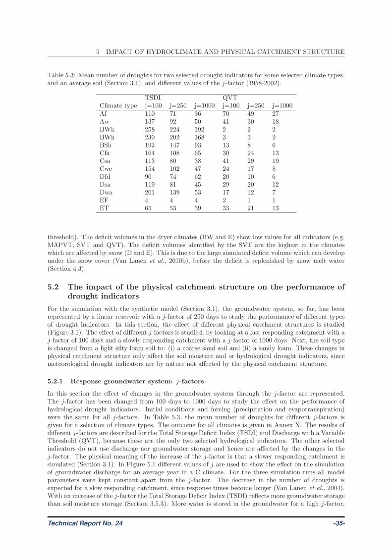
5 IMPACT OF HYDROCLIMATE AND PHYSICAL CATCHMENT STRUCTURE
Table 5.3: Mean number of droughts for two selected drought indicators for some selected climate types,and an average soil (Section 3.1), and different values of the j-factor (1958-2002).
TSDI QVTClimate type j=100 j=250 j=1000 j=100 j=250 j=1000Af 110 71 36 70 49 27Aw 137 92 50 41 30 18BWk 258 224 192 2 2 2BWh 230 202 168 3 3 2BSh 192 147 93 13 8 6Cfa 164 108 65 30 24 13Csa 113 80 38 41 29 19Cwc 154 102 47 24 17 8Dfd 90 74 62 20 10 6Dsa 119 81 45 29 20 12Dwa 201 139 53 17 12 7EF 4 4 4 2 1 1ET 65 53 39 33 21 13
threshold). The deficit volumes in the dryer climates (BW and E) show low values for all indicators (e.g.MAPVT, SVT and QVT). The deficit volumes identified by the SVT are the highest in the climateswhich are affected by snow (D and E). This is due to the large simulated deficit volume which can developunder the snow cover (Van Lanen et al., 2010b), before the deficit is replenished by snow melt water(Section 4.3).
5.2 The impact of the physical catchment structure on the performance ofdrought indicators
For the simulation with the synthetic model (Section 3.1), the groundwater system, so far, has beenrepresented by a linear reservoir with a j-factor of 250 days to study the performance of different typesof drought indicators. In this section, the effect of different physical catchment structures is studied(Figure 3.1). The effect of different j-factors is studied, by looking at a fast responding catchment with aj-factor of 100 days and a slowly responding catchment with a j-factor of 1000 days. Next, the soil typeis changed from a light silty loam soil to: (i) a coarse sand soil and (ii) a sandy loam. These changes inphysical catchment structure only affect the soil moisture and or hydrological drought indicators, sincemeteorological drought indicators are by nature not affected by the physical catchment structure.
5.2.1 Response groundwater system: j-factors
In this section the effect of changes in the groundwater system through the j-factor are represented.The j-factor has been changed from 100 days to 1000 days to study the effect on the performance ofhydrological drought indicators. Initial conditions and forcing (precipitation and evapotranspiration)were the same for all j-factors. In Table 5.3, the mean number of droughts for different j-factors isgiven for a selection of climate types. The outcome for all climates is given in Annex X. The results ofdifferent j-factors are described for the Total Storage Deficit Index (TSDI) and Discharge with a VariableThreshold (QVT), because these are the only two selected hydrological indicators. The other selectedindicators do not use discharge nor groundwater storage and hence are affected by the changes in thej-factor. The physical meaning of the increase of the j-factor is that a slower responding catchment issimulated (Section 3.1). In Figure 5.1 different values of j are used to show the effect on the simulationof groundwater discharge for an average year in a C climate. For the three simulation runs all modelparameters were kept constant apart from the j-factor. The decrease in the number of droughts isexpected for a slow responding catchment, since response times become longer (Van Lanen et al., 2004).With an increase of the j-factor the Total Storage Deficit Index (TSDI) reflects more groundwater storagethan soil moisture storage (Section 3.5.3). More water is stored in the groundwater for a high j-factor,
Technical Report No. 24 -35-
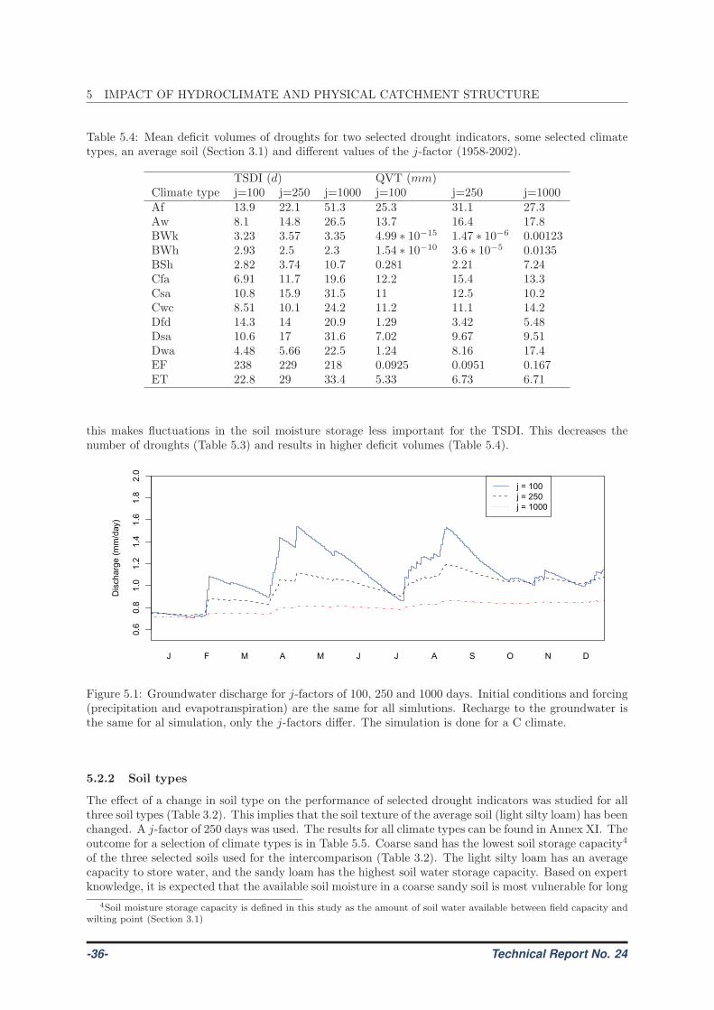
5 IMPACT OF HYDROCLIMATE AND PHYSICAL CATCHMENT STRUCTURE
Table 5.4: Mean deficit volumes of droughts for two selected drought indicators, some selected climatetypes, an average soil (Section 3.1) and different values of the j-factor (1958-2002).
TSDI (d) QVT (mm)Climate type j=100 j=250 j=1000 j=100 j=250 j=1000Af 13.9 22.1 51.3 25.3 31.1 27.3Aw 8.1 14.8 26.5 13.7 16.4 17.8BWk 3.23 3.57 3.35 4.99 ∗ 10−15 1.47 ∗ 10−6 0.00123BWh 2.93 2.5 2.3 1.54 ∗ 10−10 3.6 ∗ 10−5 0.0135BSh 2.82 3.74 10.7 0.281 2.21 7.24Cfa 6.91 11.7 19.6 12.2 15.4 13.3Csa 10.8 15.9 31.5 11 12.5 10.2Cwc 8.51 10.1 24.2 11.2 11.1 14.2Dfd 14.3 14 20.9 1.29 3.42 5.48Dsa 10.6 17 31.6 7.02 9.67 9.51Dwa 4.48 5.66 22.5 1.24 8.16 17.4EF 238 229 218 0.0925 0.0951 0.167ET 22.8 29 33.4 5.33 6.73 6.71
this makes fluctuations in the soil moisture storage less important for the TSDI. This decreases thenumber of droughts (Table 5.3) and results in higher deficit volumes (Table 5.4).
Dis
charg
e (
mm
/day)
0.6
0.8
1.0
1.2
1.4
1.6
1.8
2.0
J F M A M J J A S O N D
j = 100
j = 250
j = 1000
Figure 5.1: Groundwater discharge for j-factors of 100, 250 and 1000 days. Initial conditions and forcing(precipitation and evapotranspiration) are the same for all simlutions. Recharge to the groundwater isthe same for al simulation, only the j-factors differ. The simulation is done for a C climate.
5.2.2 Soil types
The effect of a change in soil type on the performance of selected drought indicators was studied for allthree soil types (Table 3.2). This implies that the soil texture of the average soil (light silty loam) has beenchanged. A j-factor of 250 days was used. The results for all climate types can be found in Annex XI. Theoutcome for a selection of climate types is in Table 5.5. Coarse sand has the lowest soil storage capacity4
of the three selected soils used for the intercomparison (Table 3.2). The light silty loam has an averagecapacity to store water, and the sandy loam has the highest soil water storage capacity. Based on expertknowledge, it is expected that the available soil moisture in a coarse sandy soil is most vulnerable for long
4Soil moisture storage capacity is defined in this study as the amount of soil water available between field capacity andwilting point (Section 3.1)
-36- Technical Report No. 24
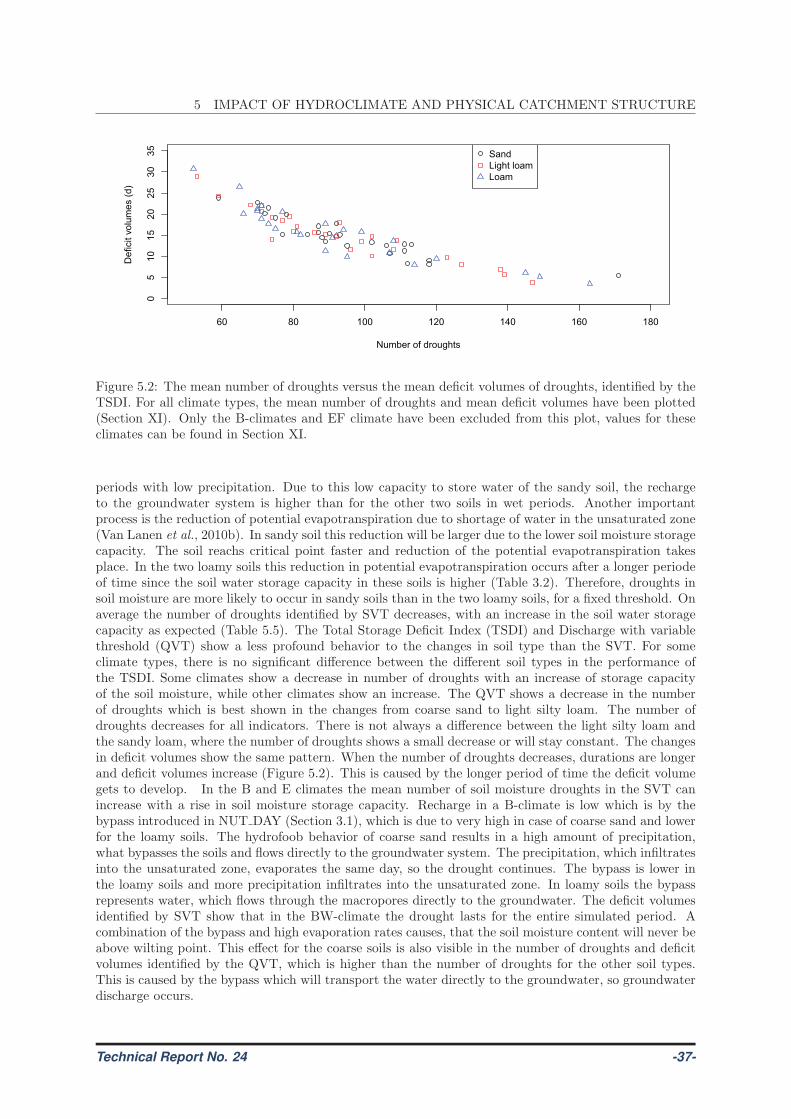
5 IMPACT OF HYDROCLIMATE AND PHYSICAL CATCHMENT STRUCTURE
60 80 100 120 140 160 180
05
10
15
20
25
30
35
Number of droughts
Deficit v
olu
mes (
d)
Sand
Light loam
Loam
Figure 5.2: The mean number of droughts versus the mean deficit volumes of droughts, identified by theTSDI. For all climate types, the mean number of droughts and mean deficit volumes have been plotted(Section XI). Only the B-climates and EF climate have been excluded from this plot, values for theseclimates can be found in Section XI.
periods with low precipitation. Due to this low capacity to store water of the sandy soil, the rechargeto the groundwater system is higher than for the other two soils in wet periods. Another importantprocess is the reduction of potential evapotranspiration due to shortage of water in the unsaturated zone(Van Lanen et al., 2010b). In sandy soil this reduction will be larger due to the lower soil moisture storagecapacity. The soil reachs critical point faster and reduction of the potential evapotranspiration takesplace. In the two loamy soils this reduction in potential evapotranspiration occurs after a longer periodeof time since the soil water storage capacity in these soils is higher (Table 3.2). Therefore, droughts insoil moisture are more likely to occur in sandy soils than in the two loamy soils, for a fixed threshold. Onaverage the number of droughts identified by SVT decreases, with an increase in the soil water storagecapacity as expected (Table 5.5). The Total Storage Deficit Index (TSDI) and Discharge with variablethreshold (QVT) show a less profound behavior to the changes in soil type than the SVT. For someclimate types, there is no significant difference between the different soil types in the performance ofthe TSDI. Some climates show a decrease in number of droughts with an increase of storage capacityof the soil moisture, while other climates show an increase. The QVT shows a decrease in the numberof droughts which is best shown in the changes from coarse sand to light silty loam. The number ofdroughts decreases for all indicators. There is not always a difference between the light silty loam andthe sandy loam, where the number of droughts shows a small decrease or will stay constant. The changesin deficit volumes show the same pattern. When the number of droughts decreases, durations are longerand deficit volumes increase (Figure 5.2). This is caused by the longer period of time the deficit volumegets to develop. In the B and E climates the mean number of soil moisture droughts in the SVT canincrease with a rise in soil moisture storage capacity. Recharge in a B-climate is low which is by thebypass introduced in NUT DAY (Section 3.1), which is due to very high in case of coarse sand and lowerfor the loamy soils. The hydrofoob behavior of coarse sand results in a high amount of precipitation,what bypasses the soils and flows directly to the groundwater system. The precipitation, which infiltratesinto the unsaturated zone, evaporates the same day, so the drought continues. The bypass is lower inthe loamy soils and more precipitation infiltrates into the unsaturated zone. In loamy soils the bypassrepresents water, which flows through the macropores directly to the groundwater. The deficit volumesidentified by SVT show that in the BW-climate the drought lasts for the entire simulated period. Acombination of the bypass and high evaporation rates causes, that the soil moisture content will never beabove wilting point. This effect for the coarse soils is also visible in the number of droughts and deficitvolumes identified by the QVT, which is higher than the number of droughts for the other soil types.This is caused by the bypass which will transport the water directly to the groundwater, so groundwaterdischarge occurs.
Technical Report No. 24 -37-
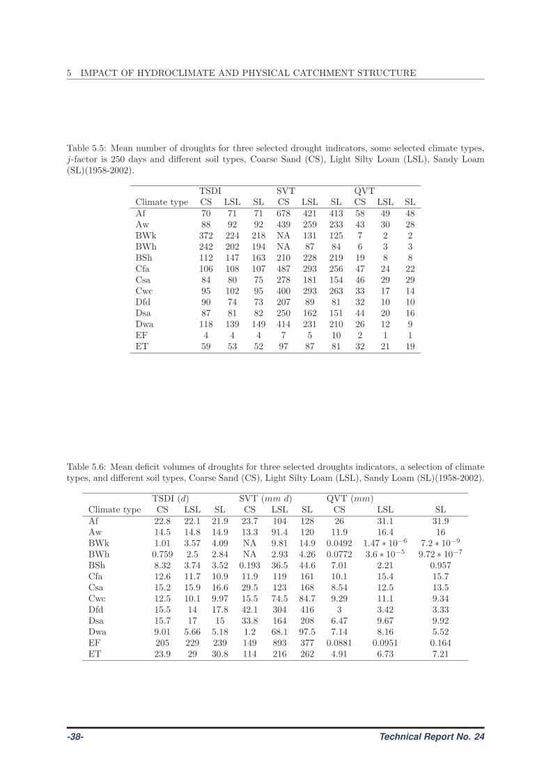
5 IMPACT OF HYDROCLIMATE AND PHYSICAL CATCHMENT STRUCTURE
Table 5.5: Mean number of droughts for three selected drought indicators, some selected climate types,j-factor is 250 days and different soil types, Coarse Sand (CS), Light Silty Loam (LSL), Sandy Loam(SL)(1958-2002).
TSDI SVT QVTClimate type CS LSL SL CS LSL SL CS LSL SLAf 70 71 71 678 421 413 58 49 48Aw 88 92 92 439 259 233 43 30 28BWk 372 224 218 NA 131 125 7 2 2BWh 242 202 194 NA 87 84 6 3 3BSh 112 147 163 210 228 219 19 8 8Cfa 106 108 107 487 293 256 47 24 22Csa 84 80 75 278 181 154 46 29 29Cwc 95 102 95 400 293 263 33 17 14Dfd 90 74 73 207 89 81 32 10 10Dsa 87 81 82 250 162 151 44 20 16Dwa 118 139 149 414 231 210 26 12 9EF 4 4 4 7 5 10 2 1 1ET 59 53 52 97 87 81 32 21 19
Table 5.6: Mean deficit volumes of droughts for three selected droughts indicators, a selection of climatetypes, and different soil types, Coarse Sand (CS), Light Silty Loam (LSL), Sandy Loam (SL)(1958-2002).
TSDI (d) SVT (mm d) QVT (mm)Climate type CS LSL SL CS LSL SL CS LSL SLAf 22.8 22.1 21.9 23.7 104 128 26 31.1 31.9Aw 14.5 14.8 14.9 13.3 91.4 120 11.9 16.4 16BWk 1.01 3.57 4.09 NA 9.81 14.9 0.0492 1.47 ∗ 10−6 7.2 ∗ 10−9
BWh 0.759 2.5 2.84 NA 2.93 4.26 0.0772 3.6 ∗ 10−5 9.72 ∗ 10−7
BSh 8.32 3.74 3.52 0.193 36.5 44.6 7.01 2.21 0.957Cfa 12.6 11.7 10.9 11.9 119 161 10.1 15.4 15.7Csa 15.2 15.9 16.6 29.5 123 168 8.54 12.5 13.5Cwc 12.5 10.1 9.97 15.5 74.5 84.7 9.29 11.1 9.34Dfd 15.5 14 17.8 42.1 304 416 3 3.42 3.33Dsa 15.7 17 15 33.8 164 208 6.47 9.67 9.92Dwa 9.01 5.66 5.18 1.2 68.1 97.5 7.14 8.16 5.52EF 205 229 239 149 893 377 0.0881 0.0951 0.164ET 23.9 29 30.8 114 216 262 4.91 6.73 7.21
-38- Technical Report No. 24
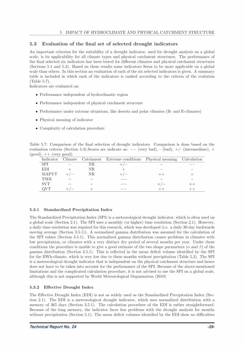
5 IMPACT OF HYDROCLIMATE AND PHYSICAL CATCHMENT STRUCTURE
5.3 Evaluation of the final set of selected drought indicators
An important criterion for the suitability of a drought indicator, used for drought analysis on a globalscale, is its applicability for all climate types and physical catchment structures. The performance ofthe final selected six indicators has been tested for different climates and physical catchment structures(Sections 5.1 and 5.2). Based on these results some indicators Seem to be more applicable on a globalscale than others. In this section an evaluation of each of the six selected indicators is given. A summarytable is included in which each of the indicators is ranked according to the criteria of the evalution(Table 5.7).Indicators are evaluated on:
• Performance independent of hydroclimatic region
• Performance independent of physical catchment structure
• Performance under extreme situations, like deserts and polar climates (B- and E-climates)
• Physical meaning of indicator
• Complexity of calculation procedure
Table 5.7: Comparison of the final selection of drought indicators. Comparison is done based on theevaluation criteria (Section 5.3).Scores are indicate as: −− (very bad), - (bad), +/- (intermediate), +(good), ++ (very good).
Indicator Climate Catchment Extreme conditions Physical meaning CalculationSPI − NR +/− − −−
EDI + NR + − −
MAPVT +/− NR +/− ++ +TSDI − − −− − −
SVT − − −− +/− ++QVT +/− + −− ++ ++
5.3.1 Standardized Precipitation Index
The Standardized Precipitation Index (SPI) is a meteorological drought indicator, which is often used ona global scale (Section 2.1). The SPI uses a monthly (or higher) time resolution (Section 2.1). However,a daily time resolution was required for this research, which was developed (i.e. a daily 30-day backwardsmoving average (Section 3.5.1)). A normalized gamma distribution was assumed for the calculation ofthe SPI values (Section 3.5.1). This normalized gamma distribution causes problems in climates withlow precipitation, or climates with a very distinct dry period of several months per year. Under theseconditions the procedure is unable to give a good estimate of the two shape parameters (α and β) of thegamma distribution (Section 3.5.1). This is reflected in the mean deficit volume identified by the SPIfor the BWh-climate, which is very low due to these months without precipitation (Table 5.2). The SPIis a meteorological drought indicator that is independent on the physical catchment structure and hencedoes not have to be taken into account for the performance of the SPI. Because of the above-mentionedlimitations and the complicated calculation procedure, it is not advised to use the SPI on a global scale,although this is not supported by World Meteorological Organization (2010)
5.3.2 Effective Drought Index
The Effective Drought Index (EDI) is not as widely used as the Standardized Precipitation Index (Sec-tion 2.1). The EDI is a meteorological drought indicator, which uses normalized distribution with amemory of 365 days (Section 3.5.1). The calculation procedure of the EDI is rather straightforward.Because of the long memory, the indicator faces less problems with the drought analysis for monthswithout precipitation (Section 5.1). The mean deficit volumes identified by the EDI show no difficulties
Technical Report No. 24 -39-
5 IMPACT OF HYDROCLIMATE AND PHYSICAL CATCHMENT STRUCTURE
for the BWh-climate or other extreme climates (Table 5.2). Therefore, the EDI is found to be a bettermeteorological drought indicator than the SPI. However, the long memory could be a disadvantage fora meteorological drought indicator, since shorter periods with low precipitation have a smaller effect onthe EDI values. Like the SPI, the EDI is independent on the physical catchment structure.
5.3.3 Moving Average Precipitation with a Variable Threshold
The last of the finally selected meteorological drought indicators was the Moving Average Precipitationwith a Variable Threshold (MAPVT). This indicator takes a 30 days centered moving average to calculatethe moving average of the precipitation (Section 3.5.1). This ensures that the MAPVT has no difficultieswith a noumber of rainless days. However, months without precipitation still pose difficulties as theaggregation period is not more than 30 days. If a particular month is without rain for more than 20%of the years, the selected 80% threshold for this month will become zero. The MAPVT, however, isnot very sensitive to these zeros since no fitting of a gamma distribution has to be done. An advantageof this drought indicator, is that the values of the MAPVT can easily be calculated without fittingor normalization. However, the threshold for the MAPVT should be calculated using long time seriesof precipitation. The mean deficit volumes of the MAPVT are strongly affected by the hydroclimate(Table 5.2). The physical meaning of the deficit volume of the MAPVT seems to be an advantagecompared to the SPI and EDI, since it can be easily calculated how much additional precipitation isrequired to recover from a particular drought event. Therefore, the MAPVT seems to be the bestmeteorological drought indicator for drought analysis on a global scale.
5.3.4 Total Storage Deficit Index
The Total Storage Deficit Index (TSDI) uses both the storage in the unsaturated zone and the groundwa-ter for drought analysis (Section 2.3). The performance of the TSDI can be studied for changes both inhydroclimate and physical catchment structure. The TSDI is a normalized combined drought indicator,which can be used for either the detection of soil moisture droughts or the detection of hydrologicaldroughts (Section 3.5.3). The climate condition can determine the performance of the TSDI as either asoil moisture or a hydrological drought indicator. If the precipitation and groundwater storage are high,the performance of the TSDI is more like a hydrological drought indicator. On the contrary, when pre-cipitation and groundwater storage are low, its performance will be like a soil moisture drought indicator(Section 3.5.3). The performance of the TSDI is very dependent on both the hydroclimate (Table 5.1)and physical catchment structure (Table 5.3 and 5.5). This is a disadvantages when the TSDI is usedon a global scale, because too much factors influence the performance of the TSDI and evaluation of theperformance is difficult. The calculation procedure of the TSDI is complicated, since soil moisture andgroundwater storage are required and all values need to be normalized. It is not advised to use the TSDIfor drought analysis on a global scale although the use of one indicator to capture all droughts presentin the unsaturated and saturated zone is a good concept.
5.3.5 Soil moisture content with a Variable Threshold
The Soil moisture content with a Variable Threshold (SVT) has been proposed in this study to detect soilmoisture droughts. Drought detection with the SVT is done with a variable threshold (Section 3.5.2).The performance of the SVT is very sensitive to the climate type (Table 5.1) and soil type (Table 5.5).This strong dependence on the soil type may cause problems. If other models are used the SVT is verysensitive to a classification of the soil type. On a global scale, the SVT has been used in several studies(Section 2.2). However, based on the results from this research, it is not advised to use the SVT fordrought analysis on a global scale.
5.3.6 Discharge with a Variable Threshold
For the detection of streamflow droughts, the Discharge with a Variable Threshold (QVT) has beenproposed in this study. A variable threshold is calculated with the use of discharge values (Section 3.5.3).The mean number of droughts for the QVT is low for every climate type compared to other indicators(Table 5.1). Without standardization the mean deficit volumes of the QVT have a large variationbetween hydroclimates (Table 5.2). The deficit volumes indentified by the QVT do have the same
-40- Technical Report No. 24
5 IMPACT OF HYDROCLIMATE AND PHYSICAL CATCHMENT STRUCTURE
physical meaning as those indentified by the MAPVT. Months without discharge for more than 20% ofthe years cause difficulties for the application of the QVT, since the 80% threshold will become zero.However, months without discharge are less common than for precipitation, so this problem will occurless often. The QVT seems to be the most promising indicator from all the non-meteorological droughtindicators, because it is capable of dealing with dry climates and its physical meaning of the deficitvolume.
Technical Report No. 24 -41-

5 IMPACT OF HYDROCLIMATE AND PHYSICAL CATCHMENT STRUCTURE
-42- Technical Report No. 24
6 DISCUSSION
6 Discussion
In this study the most important assumptions and their uncertainties are discussed in the context of theassessment of the performance of the drought indicators across the world.
6.1 Synthetic model
The synthetic model NUT DAY uses some simplifications for the simulation of rainfall-runoff process(Section 3.1). These simplifications allowed to perform lots of calculations that were required for thisstudy. However, due to these simplifications some physical processes are not captured well by NUT DAY,which might affect the simulated of runoff. The most important simplifications of the NUT DAY arementioned below.
6.1.1 Soil moisture simulation
The first simplification is the use of a single soil box for the simulation of the soil moisture storagealthough a two-layer soil profile is used to define the soil moisture supply capacity(Section 3.1). Novertical distribution of for the soil moisture profile is made, which results in no difference between thevolumetric water content at the top and the bottom of the soil (Van Lanen et al., 2010b). The subsoiland topsoil defined in NUT DAY are combined into one soil box (lumped, vertical model), which doesnot address soil moisture content gradients and a possible limiting maximum infiltration rate at thesurface (Van Lanen et al., 2010b). This may effect the simulated soil water balance, especially the rootwater uptake (i.e. actual evapotranspiration) and the bypass. After a long period without precipitation,the topsoil would be very dry due to evapotranspiration in reality (Van Lanen et al., 2004), whereasNUT DAY does not take this into account and the grass crop may still transpire at a potential rate ifthe total soil moisture storage is sufficient.
6.1.2 Linear reservoir
In NUT DAY, a single reservoir is used for the simulation of discharge, of which the outflow rate isdetermined by the De Zeeuw-Hellinga approach (Ritzema, 1994). Compared to some other models,which use multiple reservoirs, the current version of NUT DAY is unable to simulate a slow flow and aquick flow component at the same time. NUT DAY is designed to simulate groundwater discharge only.Fast components like surface runoff and shallow saturated subsurface flow (interflow) are not capturedby the model. However, some adjustments (Section 3.1.3) have been made to make the current versionof NUT DAY more suited for the simulation of the fast groundwater fluctuations caused by precipitationevents with a high intensity (e.g. bypass, recharge even if the soil is dryer than field capacity).
6.1.3 Bypass
Bypass in NUT DAY is activated when a heavy precipitation event occurs and the soil is very dry(Section 3.1). It is assumed that the precipitation infiltration cannot exceed a maximum rate. In thisstudy, this maximum rate is set at the hydraulic conductivity at field capacity. If the daily precipitationexceeds the maximum infiltration rate, bypass is assumed to occur. A second assumption is that bypassis only active when the soil moisture storage is below a critical point (Table 3.2). In these situations, it isassumed that cracks and macro-pores in the soil transport part of the water directly to the groundwater(Section 3.1.4). When the soil is wetter than critical point, all precipitation is assumed to infiltrateinto the unsaturated soil. With this bypass approach the response of the groundwater system to heavyprecipitation is simulated better with NUT DAY, but it does not imply that NUT DAY simulates fastrunoff components (Van Lanen et al., 2010b).
6.2 Soil types
The soils used in this research were retrieved from the Staring Series (Wosten et al., 2001). The selectionof the soils (Table 3.2) was done from a total of 22 standard soils. These soils were used to identify afew representative soil types which likely can be found acros the world. In this study, three differentsoil textures have been used; a soil with a low, medium and high soil moisture storage capacity. The
Technical Report No. 24 -43-
6 DISCUSSION
selection of these soil textures was based on the total amount of water available between wilting pointen field capacity. Peat soils are excluded from the selection because of their specific characteristics (veryhigh soil moisture storage capacity, dynamic behavior).The selected rooting depth of 50 cm in this study reflects the rooting depth of grass. However, in someregions across the world this rooting depth will never be reached due to shallow bedrock or permafrost.In regions, where other vegetation than grass is dominant, rooting depths can be even over 200 cm in caseno penetration resistant layer occurs (e.g. Schenka & Jackson (2005)). A thicker soil has large effects onthe soil moisture capacity and the actual evapotranspiration rates, especially in dryer climates. If rootingdepths is larger, the capacity to store water in the unsaturated zone and the actual evapotranspirationincrease and the other way around. However, there is a limitation to this process. If rooting depthbecomes very large, evapotranspiration will never be reduced because there is enough water stored inthe unsaturated zone to overcome very dry periods (Van Lanen et al., 2004). The smaller the storagecapacity, the more droughts occur (Section 5.2.2). So, the selected rooting depth may have a profoundeffect on the magnitude of the drought characteristics and drought indicator performance.
6.3 Koppen-Geiger classification
The Koppen-Geiger classification is a well-known, but a rather old climate classification (Koppen, 1900).Adjustments to the Koppen-Geiger classification have been made by Geiger (1954). The Koppen-Geigerclassification is a discrete classification based only on precipitation and temperature. However, other clas-sifications (e.g. Holdridge life zones, Holdridge (1947); Thornthwaite climate classification, Thornthwaite(1948)) are available, and may be better suited to give a climate classification on a global scale.
6.4 Drought concept
Droughts are caused by situations with less than normal water availability. They are present in everyhydroclimatic region and appear in different components of the hydrological cycle (Wilhite, 2000). Thismeans that locations, where water is (almost) never available, have an extremely low normal wateravailability and the threshold will be very low or even zero. These cases should not be called a droughtanymore, but it refers to aridity (permanently dry). This also affects the way droughts have to be studied.If NUT DAY is used for the simulation of soil moisture and groundwater discharge, soil moisture andhydrological drought indicators should not be used, for the very dry climates, like the BW-climates. Inthese regions very deep groundwater storage is possible (Stahl & Hisdal, 2004). However, due to modelstructure of NUT DAY this deep groundwater storage cannot be simulated (model does not distinguishshallow and deep groundwater storage) (Van Lanen et al., 2010b). As long as there is precipitation formost of the years, meteorological drought indicators can still be applied (especially the Effective DroughtIndex (EDI) and Consecutive Dry Days (CDD)). The CDD is very suited for drought definition in dryclimates since it particularly addresses very long dry periods (Section 4.2). However, in wetter climatesthe CDD is not so useful for the detection of droughts (Section 4.2).In the EF-climate all precipitation is accumulated as snow and will melt only when temperatures areabove 0◦C, which is very rare. Soil moisture is also heavily affected by the frozen soils in these climates.These locations (mostly situated on the poles and Greenland) give rise to difficulties for all indicators,except for those which focus only on precipitation. So, streamflow and soil moisture drought indicatorsface difficulties in the EF-climate, where streamflow is (almost) absent due to average monthly tem-peratures which are always below 0◦C. The BW-climate and EF-climate were included in this researchbecause drought can still be detected with the use of (some) precipitation drought indicators.
-44- Technical Report No. 24
7 CONCLUSIONS AND RECOMMENDATIONS
7 Conclusions and recommendations
7.1 Conclusions
This study on the performance of drought indicators on the large scale led to the following conclusions:
• For drought analysis on a global scale, both the Moving Average Precipitation with a VariableThreshold (MAPVT) and the Discharge with a Variable Threshold (QVT) are found to be promis-ing drought indicators. The combined use of the MAPVT and QVT allows detection of bothmeteorological and hydrological droughts and enables intercomparison (Sections 3.5.1 and 3.5.3).The MAPVT and QVT have the advantage, that they are also applicable for drought analysison a more detailed scale than the global scale. When the threshold can be calculated using datafrom previous years, real-time drought monitoring on a daily basis can be done with the QVTand MAPVT, without the use of a difficult calculation procedure(Sections 3.5.1 and 3.5.3). Sinceprecipitation and discharge data are widely available this is very useful. Although the QVT hasdifficulties in very dry, B-climates, it is still selected since all hydrological drought indicators showweak performance in these B-climates (Section 5.1). The MAPVT and QVT are easy to implementand have deficit volumes which have a physical meaning that can be interpreted without difficulties.
• The Standardized Precipitation Index (SPI) faces problems with fitting the gamma-distribution forlocations with regularly dry months (Section 3.5.1). There, the estimated α and β parameters ofthe gamma distribution, are less reliable than a threshold directly derived from the precipitationas done in the MAPVT (Section 5.3).
• In very dry climates (e.g. BW-climates), the long memory of the Effective Drought Index (EDI)is a major advantage for the performance, because the EDI can easily deal with multiple monthswithout precipitation (Section 3.5.1). In these dry periods the EDI considers previous rainfall (upto 365 days back). Therefore, the EDI does not have difficulties at these sites as the SPI and theMAPVT have (Section 5.3).
• The EDI and the MAPVT have a very similar performance (Section 5.3). However, due to thevery long memory of the EDI, the MAPVT is preferred for most climate types rather than theEDI. The long memory of the EDI causes a very slow response to new precipitation events, whichis not to be expected for meteorological drought indicators (Section 3.5.1). However, the EDI isfound to be a better precipitation drought indicator than the SPI since no fitting problems occur(Section 3.5.1).
• The performances of the Soil moisture with a Variable Threshold (SVT) and Total Storage DeficitIndex (TSDI) and their associated drought characteristics are very dependent on the selectedsoil type (Section 5.2.2). For intercomparison studies on a global scale, SVT and TSDI are onlymeaningful if an adequate soil map with reliable soil textures and associated hydraulic propertieswould become available. Although it is recognized that this dependency is one of the strongproperties of the TSDI and SVT, it is found to be a negative property for an intercomparison ofdrought characteristics on a global scale as long as no adequate soil information becomes available.
• The climate type has a very large effect on the magnitude of all drought characteristics predictedwith different drought indicators (Section 5.1).
• Groundwater systems have a larger effect on the magnitude of drought characteristics as predictedwith hydrological or combined drought indicators than soil types for, independent of the hydrocli-matic region.
7.2 Recommendations
The study leads to the following recommendations:
• Identification of a standardized deficit volume for MAPVT and QVT, would improve intercom-parison of drought characteristics across the globe. So far, drought characteristics for differenthydroclimatic regions can only be reasonably compared based on durations and number of events,
Technical Report No. 24 -45-
7 CONCLUSIONS AND RECOMMENDATIONS
which are highly negatively correlated. Without standardization of the deficit volume, comparisonof drought severity (i.e. deficit volumes and intensity) can only be done in a qualitative manner.The identification of a standardized deficit volume offers an additional quantitative measure for in-tercomparison of droughts in different hydroclimates and regions with different physical catchmentstructures.
• Examination of the drought characteristics predicted with the six, finally selected drought indicators(SPI, EDI, TSDI, MAPVT, SVT and QVT) with observed data from river basins. It needs tobe investigated if the use of observed data instead of simulated data with a hydrological modelcould lead to a different performance of the drought indicators. Especially, soil moisture droughtindicators could show different performance for observed soil moisture data.
• Running the MAPVT and the QVT for all cells (about 70 000) instead of the 961 cells in this study(Section 5.1) gives a more comprehensive insight in the performance of both indicators on a globalscale. This can be done for a light silty loam soil and a linear reservoir with a j-factor of 250 days.This to get an impression of the distribution of drought characteristics within a climate region.
• Use of other climate classifications than the Kppen-Geiger climate classification. Continuous clas-sifications like the classifications of Holdridge (1947) and Thornthwaite (1948) could give a betterpicture of the spatial distribution of drought indicator performance across the world. The prob-lem by applying the Kppen-Geiger climate classification is introduced by the discrete distribution.Continuous classifications can cope with inhomogeneity within climate types.
• Application of another threshold. The 80% threshold was selected for this study. This thresholdimplies that 20% of the time a particular location will be in drought. The effect of the choice ofanother threshold on the performance of drought indicators needs to be investigated. For instance,if a 70% threshold would have been chosen, some small flow peaks that caused the end of droughtevent applying a 80% threshold would not be effective anymore.
• Investigation of the effect of the rooting depth on the performance of drought indicators. In thisstudy a rooting depth used of 50 cm was used, which reflects the rooting depth of grass (Van Lanenet al., 2010b). Cropland or other vegetation types usually have another rooting depth. Layers witha high penetration resistance (e.g. shallow bedrock) also affect rooting depth.
• Use of other climate datasets (e.g. NCEP/NCAR, (Kalnay et al., 1996)) to explore the effect ofother meteorological input data. This could in the first place lead to a different classification ofthe climate. Secondly, drought indicator performance could also be affected.
• Use another method to identify drought events and its associated characteristics. In this study thethreshold method was used, which is has a duration nature. The 80% threshold was used in thisstudy, which means that the flux or state is equaled or exceeded to 80% of the time. For example,Peters et al. (2003) propose a volume-based criterion.
• Use of a Global Hydrological Model (GHM) or a Land Surface Model (LSM) instead of the syntheticmodel in this study. GHMs and LSMs use a more or less simplified representation of the actualsoil and groundwater system for each cell.
• Further examination of, in particular the dependence between MAPVT and QVT (Annex III), andhow droughts in precipitation are related to discharge droughts. The MAPVT and the QVT couldbe used for this purpose since both indicators have the same physical dimensions and calculationprocedure (Sections 3.5.1 and 3.5.3). Understanding the mechanism of drought propagation willsubstantially increase the relevance of drought forecasting, since hydrological droughts can then bepredicted from droughts in precipitation.
• Investigation of the performance of MAPVT, using another moving average. In this study, the30 day centered moving average was used (Section 3.5.1). However, for real-time monitoring thisapproach would not work, since no future data are available. Hence, the moving average of theprevious 30 days is proposed.
-46- Technical Report No. 24
7 CONCLUSIONS AND RECOMMENDATIONS
• Compare the drought characteristics of both the original classification of the SPI (Table 3.4) andof the drought selected with the threshold method (Section 3.4). Severe and extreme droughtsdetermined with the SPI can be compared with the droughts identified with the threshold method.This comparison will demonstrate if the discrete approach of the SPI is suited for drought detection.
• Use of continuous climate classification systems for impact studies. These systems offer the oppor-tunity to determine mathematical relations between drought characteristics (e.g. average droughtdeficit volume) and climate variables (e.g. precipitation). With these relations, for example, theeffect of climate change (e.g. higher precipitation) could be explored.
Technical Report No. 24 -47-

7 CONCLUSIONS AND RECOMMENDATIONS
-48- Technical Report No. 24
REFERENCES
References
Agboma, C.O., Yirdaw, S.Z., & Snelgrove, K.R. 2009. Intercomparison of the Total Storage Deficit Index(TSDI) over two Canadian Prairie catchments. Journal of Hydrology, 374, 351 – 359.
Allen, R.G., Pereira, L.S., Raes, D., & Smith, M. 2006. FAO Irrigation and Drainage Paper No. 56 -Crop Evapotranspiration. Food and Agriculture Organization.
Alley, W.M. 1984. The Palmer Drought Severity Index: Limitations and Assumptions. Journal ofClimate and Applied Meteorology, 23, 1100 – 1109.
Byun, H.R., & Wilhite, D.A. 1999. Objective quantification of drought severity and duration. Bulletinof the American Meteorological Society, 12, 2747 – 2756.
Cutore, P., Di Mauro, G., & Cancelliere, A. 2009. Forecasting Palmer Index using neural networks andclimatic indexes. Journal of Hydrologic Engineering, 14, 588 – 595.
Dai, A., Trenberth, K.E., & Qian, T. 2004. A global dataset of Palmer Drought Severity Index for 1870- 2002: Relationship with soil moisture and effects of surface warming. Journal of Hydrometeorology,5, 1117 – 1130.
Deni, S.M., & Jemain, A.A. 2009. Mixed log series geometric distribution for sequences of dry days.Atmospheric Research, 92, 236 – 243.
Dracup, J.A., Lee, K.S., & Paulson Jr, E.G. 1980. On the definition of droughts. Water ResourcesResearch, 16(2), 297 – 302.
Edwards, D.C., & McKee, T.B. 1997. Characteristics of 20th century drought in the United States atmultiple time scales. Climatology Report, 97-2, Department of Atmospheric Science, Colorado stateUniversity, Fort Collins.
Fleig, A.K., Tallaksen, L.M., Hisdal, H., & Demuth, S. 2006. A global evaluation of streamflow droughtcharacteristics. Hydrology and Earth System Sciences, 10, 535 – 552.
Foley, J.C. 1957. Droughts in Australia : review of records from earliest years of settlement. AustralianBureau of Meteorology.
Fuchs, T. 2008. GPCC Annual Report for year 2008. Annual report. available at: reports and publicationssection of the GPCC homepage - gpcc.dwd.de.
Garen, D.C. 1992. Revised Surface-Water Supply Index for western United States. Journal of WaterResources Planning and Management, 119, 437 – 454.
Geiger, R. 1954. Landolt-Bornstein. Chap. Klassifikation der Klimate nach W. Kppen, pages 603 – 607of: Zahlenwerte und Funktionen aus Physik, Chemie, Astronomie, Geophysik un Technik. alte Serie,vol. 3. Springer, Berlin.
Geiger, R. 1961. Uberarbeitete Neuausgabe von Geiger, R.: Koppen-Geiger / Klima der Erde. Wandkarte1:16 Mill. Klett-Perthes, Gotha.
Gibbs, W.J., & Maher, J.V. 1967. Rainfall deciles as drought indicators. Australian Bureau of Meteo-rology.
Guttman, N.B. 1999. Accepting the Standardized Precipitation Index: A calculation algorithm. Journalof the American Water Resource Association, 35, 311 – 322.
Hayes, M.J. 1999. Drought Indices. http://www.geology.um.maine.edu/ges121/lectures/22-drought/indices1.pdf, viewed on 30-11-2009. National Drought Mitigation Center.
Hayes, M.J. 2006. What is Drought?: Drought indices. http://drought.unl.edu/whatis/indices.htm,viewed on 01-12-2009. National Drought Mitigation Center.
Technical Report No. 24 -49-
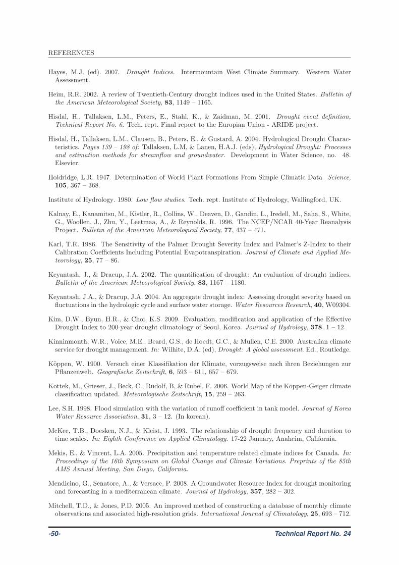
REFERENCES
Hayes, M.J. (ed). 2007. Drought Indices. Intermountain West Climate Summary. Western WaterAssessment.
Heim, R.R. 2002. A review of Twentieth-Century drought indices used in the United States. Bulletin ofthe American Meteorological Society, 83, 1149 – 1165.
Hisdal, H., Tallaksen, L.M., Peters, E., Stahl, K., & Zaidman, M. 2001. Drought event definition,Technical Report No. 6. Tech. rept. Final report to the Europian Union - ARIDE project.
Hisdal, H., Tallaksen, L.M., Clausen, B., Peters, E., & Gustard, A. 2004. Hydrological Drought Charac-teristics. Pages 139 – 198 of: Tallaksen, L.M, & Lanen, H.A.J. (eds), Hydrological Drought: Processesand estimation methods for streamflow and groundwater. Development in Water Science, no. 48.Elsevier.
Holdridge, L.R. 1947. Determination of World Plant Formations From Simple Climatic Data. Science,105, 367 – 368.
Institute of Hydrology. 1980. Low flow studies. Tech. rept. Institute of Hydrology, Wallingford, UK.
Kalnay, E., Kanamitsu, M., Kistler, R., Collins, W., Deaven, D., Gandin, L., Iredell, M., Saha, S., White,G., Woollen, J., Zhu, Y., Leetmaa, A., & Reynolds, R. 1996. The NCEP/NCAR 40-Year ReanalysisProject. Bulletin of the American Meteorological Society, 77, 437 – 471.
Karl, T.R. 1986. The Sensitivity of the Palmer Drought Severity Index and Palmer’s Z-Index to theirCalibration Coefficients Including Potential Evapotranspiration. Journal of Climate and Applied Me-teorology, 25, 77 – 86.
Keyantash, J., & Dracup, J.A. 2002. The quantification of drought: An evaluation of drought indices.Bulletin of the American Meteorological Society, 83, 1167 – 1180.
Keyantash, J.A., & Dracup, J.A. 2004. An aggregate drought index: Assessing drought severity based onfluctuations in the hydrologic cycle and surface water storage. Water Resources Research, 40, W09304.
Kim, D.W., Byun, H.R., & Choi, K.S. 2009. Evaluation, modification and application of the EffectiveDrought Index to 200-year drought climatology of Seoul, Korea. Journal of Hydrology, 378, 1 – 12.
Kinninmonth, W.R., Voice, M.E., Beard, G.S., de Hoedt, G.C., & Mullen, C.E. 2000. Australian climateservice for drought management. In: Wilhite, D.A. (ed), Drought: A global assessment. Ed., Routledge.
Koppen, W. 1900. Versuch einer Klassifikation der Klimate, vorzugsweise nach ihren Beziehungen zurPflanzenwelt. Geografische Zeitschrift, 6, 593 – 611, 657 – 679.
Kottek, M., Grieser, J., Beck, C., Rudolf, B, & Rubel, F. 2006. World Map of the Koppen-Geiger climateclassification updated. Meteorologische Zeitschrift, 15, 259 – 263.
Lee, S.H. 1998. Flood simulation with the variation of runoff coefficient in tank model. Journal of KoreaWater Resource Association, 31, 3 – 12. (In korean).
McKee, T.B., Doesken, N.J., & Kleist, J. 1993. The relationship of drought frequency and duration totime scales. In: Eighth Conference on Applied Climatology. 17-22 January, Anaheim, California.
Mekis, E., & Vincent, L.A. 2005. Precipitation and temperature related climate indices for Canada. In:Proceedings of the 16th Symposium on Global Change and Climate Variations. Preprints of the 85thAMS Annual Meeting, San Diego, California.
Mendicino, G., Senatore, A., & Versace, P. 2008. A Groundwater Resource Index for drought monitoringand forecasting in a mediterranean climate. Journal of Hydrology, 357, 282 – 302.
Mitchell, T.D., & Jones, P.D. 2005. An improved method of constructing a database of monthly climateobservations and associated high-resolution grids. International Journal of Climatology, 25, 693 – 712.
-50- Technical Report No. 24
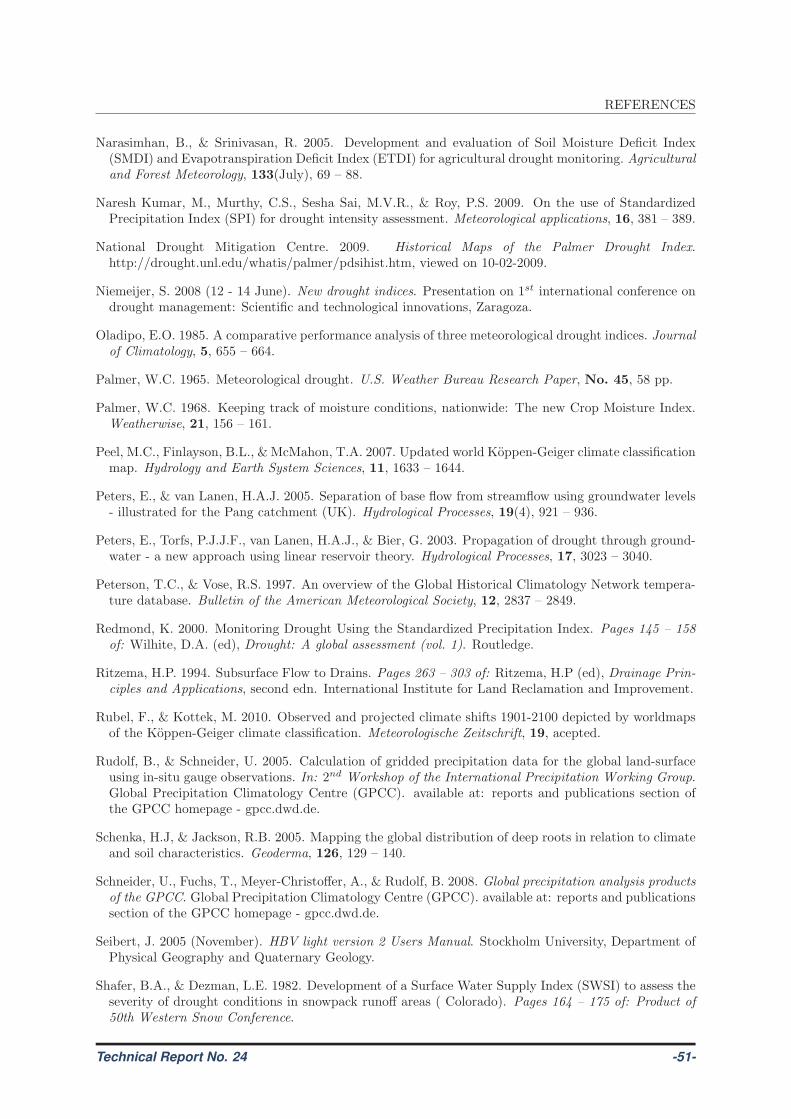
REFERENCES
Narasimhan, B., & Srinivasan, R. 2005. Development and evaluation of Soil Moisture Deficit Index(SMDI) and Evapotranspiration Deficit Index (ETDI) for agricultural drought monitoring. Agriculturaland Forest Meteorology, 133(July), 69 – 88.
Naresh Kumar, M., Murthy, C.S., Sesha Sai, M.V.R., & Roy, P.S. 2009. On the use of StandardizedPrecipitation Index (SPI) for drought intensity assessment. Meteorological applications, 16, 381 – 389.
National Drought Mitigation Centre. 2009. Historical Maps of the Palmer Drought Index.http://drought.unl.edu/whatis/palmer/pdsihist.htm, viewed on 10-02-2009.
Niemeijer, S. 2008 (12 - 14 June). New drought indices. Presentation on 1st international conference ondrought management: Scientific and technological innovations, Zaragoza.
Oladipo, E.O. 1985. A comparative performance analysis of three meteorological drought indices. Journalof Climatology, 5, 655 – 664.
Palmer, W.C. 1965. Meteorological drought. U.S. Weather Bureau Research Paper, No. 45, 58 pp.
Palmer, W.C. 1968. Keeping track of moisture conditions, nationwide: The new Crop Moisture Index.Weatherwise, 21, 156 – 161.
Peel, M.C., Finlayson, B.L., & McMahon, T.A. 2007. Updated world Koppen-Geiger climate classificationmap. Hydrology and Earth System Sciences, 11, 1633 – 1644.
Peters, E., & van Lanen, H.A.J. 2005. Separation of base flow from streamflow using groundwater levels- illustrated for the Pang catchment (UK). Hydrological Processes, 19(4), 921 – 936.
Peters, E., Torfs, P.J.J.F., van Lanen, H.A.J., & Bier, G. 2003. Propagation of drought through ground-water - a new approach using linear reservoir theory. Hydrological Processes, 17, 3023 – 3040.
Peterson, T.C., & Vose, R.S. 1997. An overview of the Global Historical Climatology Network tempera-ture database. Bulletin of the American Meteorological Society, 12, 2837 – 2849.
Redmond, K. 2000. Monitoring Drought Using the Standardized Precipitation Index. Pages 145 – 158of: Wilhite, D.A. (ed), Drought: A global assessment (vol. 1). Routledge.
Ritzema, H.P. 1994. Subsurface Flow to Drains. Pages 263 – 303 of: Ritzema, H.P (ed), Drainage Prin-ciples and Applications, second edn. International Institute for Land Reclamation and Improvement.
Rubel, F., & Kottek, M. 2010. Observed and projected climate shifts 1901-2100 depicted by worldmapsof the Koppen-Geiger climate classification. Meteorologische Zeitschrift, 19, acepted.
Rudolf, B., & Schneider, U. 2005. Calculation of gridded precipitation data for the global land-surfaceusing in-situ gauge observations. In: 2nd Workshop of the International Precipitation Working Group.Global Precipitation Climatology Centre (GPCC). available at: reports and publications section ofthe GPCC homepage - gpcc.dwd.de.
Schenka, H.J, & Jackson, R.B. 2005. Mapping the global distribution of deep roots in relation to climateand soil characteristics. Geoderma, 126, 129 – 140.
Schneider, U., Fuchs, T., Meyer-Christoffer, A., & Rudolf, B. 2008. Global precipitation analysis productsof the GPCC. Global Precipitation Climatology Centre (GPCC). available at: reports and publicationssection of the GPCC homepage - gpcc.dwd.de.
Seibert, J. 2005 (November). HBV light version 2 Users Manual. Stockholm University, Department ofPhysical Geography and Quaternary Geology.
Shafer, B.A., & Dezman, L.E. 1982. Development of a Surface Water Supply Index (SWSI) to assess theseverity of drought conditions in snowpack runoff areas ( Colorado). Pages 164 – 175 of: Product of50th Western Snow Conference.
Technical Report No. 24 -51-
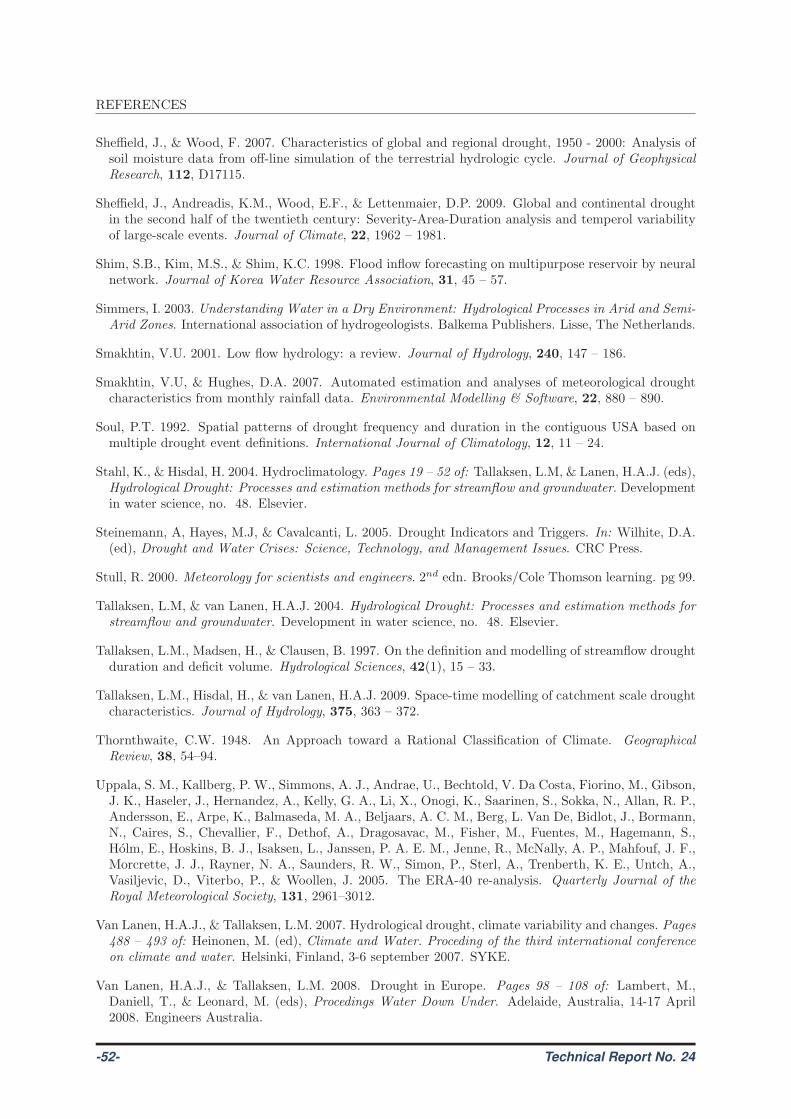
REFERENCES
Sheffield, J., & Wood, F. 2007. Characteristics of global and regional drought, 1950 - 2000: Analysis ofsoil moisture data from off-line simulation of the terrestrial hydrologic cycle. Journal of GeophysicalResearch, 112, D17115.
Sheffield, J., Andreadis, K.M., Wood, E.F., & Lettenmaier, D.P. 2009. Global and continental droughtin the second half of the twentieth century: Severity-Area-Duration analysis and temperol variabilityof large-scale events. Journal of Climate, 22, 1962 – 1981.
Shim, S.B., Kim, M.S., & Shim, K.C. 1998. Flood inflow forecasting on multipurpose reservoir by neuralnetwork. Journal of Korea Water Resource Association, 31, 45 – 57.
Simmers, I. 2003. Understanding Water in a Dry Environment: Hydrological Processes in Arid and Semi-Arid Zones. International association of hydrogeologists. Balkema Publishers. Lisse, The Netherlands.
Smakhtin, V.U. 2001. Low flow hydrology: a review. Journal of Hydrology, 240, 147 – 186.
Smakhtin, V.U, & Hughes, D.A. 2007. Automated estimation and analyses of meteorological droughtcharacteristics from monthly rainfall data. Environmental Modelling & Software, 22, 880 – 890.
Soul, P.T. 1992. Spatial patterns of drought frequency and duration in the contiguous USA based onmultiple drought event definitions. International Journal of Climatology, 12, 11 – 24.
Stahl, K., & Hisdal, H. 2004. Hydroclimatology. Pages 19 – 52 of: Tallaksen, L.M, & Lanen, H.A.J. (eds),Hydrological Drought: Processes and estimation methods for streamflow and groundwater. Developmentin water science, no. 48. Elsevier.
Steinemann, A, Hayes, M.J, & Cavalcanti, L. 2005. Drought Indicators and Triggers. In: Wilhite, D.A.(ed), Drought and Water Crises: Science, Technology, and Management Issues. CRC Press.
Stull, R. 2000. Meteorology for scientists and engineers. 2nd edn. Brooks/Cole Thomson learning. pg 99.
Tallaksen, L.M, & van Lanen, H.A.J. 2004. Hydrological Drought: Processes and estimation methods forstreamflow and groundwater. Development in water science, no. 48. Elsevier.
Tallaksen, L.M., Madsen, H., & Clausen, B. 1997. On the definition and modelling of streamflow droughtduration and deficit volume. Hydrological Sciences, 42(1), 15 – 33.
Tallaksen, L.M., Hisdal, H., & van Lanen, H.A.J. 2009. Space-time modelling of catchment scale droughtcharacteristics. Journal of Hydrology, 375, 363 – 372.
Thornthwaite, C.W. 1948. An Approach toward a Rational Classification of Climate. GeographicalReview, 38, 54–94.
Uppala, S. M., Kallberg, P. W., Simmons, A. J., Andrae, U., Bechtold, V. Da Costa, Fiorino, M., Gibson,J. K., Haseler, J., Hernandez, A., Kelly, G. A., Li, X., Onogi, K., Saarinen, S., Sokka, N., Allan, R. P.,Andersson, E., Arpe, K., Balmaseda, M. A., Beljaars, A. C. M., Berg, L. Van De, Bidlot, J., Bormann,N., Caires, S., Chevallier, F., Dethof, A., Dragosavac, M., Fisher, M., Fuentes, M., Hagemann, S.,Holm, E., Hoskins, B. J., Isaksen, L., Janssen, P. A. E. M., Jenne, R., McNally, A. P., Mahfouf, J. F.,Morcrette, J. J., Rayner, N. A., Saunders, R. W., Simon, P., Sterl, A., Trenberth, K. E., Untch, A.,Vasiljevic, D., Viterbo, P., & Woollen, J. 2005. The ERA-40 re-analysis. Quarterly Journal of theRoyal Meteorological Society, 131, 2961–3012.
Van Lanen, H.A.J., & Tallaksen, L.M. 2007. Hydrological drought, climate variability and changes. Pages488 – 493 of: Heinonen, M. (ed), Climate and Water. Proceding of the third international conferenceon climate and water. Helsinki, Finland, 3-6 september 2007. SYKE.
Van Lanen, H.A.J., & Tallaksen, L.M. 2008. Drought in Europe. Pages 98 – 108 of: Lambert, M.,Daniell, T., & Leonard, M. (eds), Procedings Water Down Under. Adelaide, Australia, 14-17 April2008. Engineers Australia.
-52- Technical Report No. 24
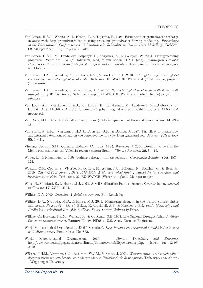
REFERENCES
Van Lanen, H.A.J., Weerts, A.H., Kroon, T., & Dijksma, R. 1996. Estimation of groundwater rechargein areas with deep groundwater tables using transient groundwater flowing modelling. Proceedingsof the International Conference on ’Calibration adn Reliability in Groundwater Modelling’, Golden,
USA(September 1996), Pages 307 – 316.
Van Lanen, H.A.J., M., Fendekova, Kupczyk, E., Kasprzyk, A., & Pokojski, W. 2004. Flow generatingprocesses. Pages 53 – 98 of: Tallaksen, L.M, & van Lanen, H.A.J. (eds), Hydrological Drought:Processes and estimation methods for streamflow and groundwater. Development in water science, no.48. Elsevier.
Van Lanen, H.A.J., Wanders, N, Tallaksen, L.M., & van Loon, A.F. 2010a. Drought analysis on a globalscale using a synthetic hydrological model. Tech. rept. EU WATCH (Water and global Change) project.(in progress).
Van Lanen, H.A.J., Wanders, N, & van Loon, A.F. 2010b. Synthetic hydrological model - illustrated withdrought using Watch Forcing Data. Tech. rept. EU WATCH (Water and global Change) project. (inprogress).
Van Loon, A.F., van Lanen, H.A.J., van Hisdal, H., Tallaksen, L.M., Fendekova, M., Oosterwijk, J.,Horvat, O., & Machlica, A. 2010. Understanding hydrological winter drought in Europe. IAHS Publ,accepted.
Van Rooy, M.P. 1965. A Rainfall anomaly index (RAI) independent of time and space. Notos, 14, 43 –48.
Van Stiphout, T.P.J., van Lanen, H.A.J., Boersma, O.H., & Bouma, J. 1987. The effect of bypass flowand internal catchment of rain on the water regime in a clay loam grassland soil. Journal of Hydrology,95, 1 – 11.
Vincente-Serrano, S.M., Gonzalez-Hidalgo, J.C., Luis, M., & Raventos, J. 2004. Drought pattern in theMediterranean area: the Valencia region (eastern Spain). Climate Research, 26, 5 – 15.
Weber, L., & Nkemdirim, L. 1998. Palmer’s drought indices revisited. Geografiska Annaler, 80A, 153 –172.
Weedon, G.P., Gomes, S., Viterbo, P., Osterle, H., Adam, J.C., Bellouin, N., Boucher, O., & Best, M.2010. The WATCH Forcing Data 1958-2001: A Meteorological forcing dataset for land surface- andhydrological models. Tech. rept. 22. EU WATCH (Water and global Change) project.
Wells, N., Goddard, S., & Hayes, M.J. 2004. A Self-Calibrating Palmer Drought Severity Index. Journalof Climate, 17, 2335 – 2351.
Wilhite, D.A. 2000. Drought: A global assessment. Ed., Routledge.
Wilhite, D.A., Svoboda, M.D., & Hayes, M.J. 2005. Monitoring drought in the United States: statusand trends. Pages 121 – 131 of: Boken, K, Cracknell, A.P., & Heathcote, R.L. (eds), Monitoring andPredicting Agricultural Drought: A Global Study. Oxford University Press.
Willeke, G., Hosking, J.R.M., Wallis, J.R., & Guttman, N.B. 1994. The National Drought Atlas. Institutefor water resources report, Report No 94-NDS-4, U.S. Army Corps of Engineers.
World Meteorological Organization. 2009 (December). Experts agree on a universal drought index to copewith climate risks. Press release No. 872.
World Meteorological Organization. 2010. Climate Variability and Extremes.http://www.wmo.int/pages/themes/climate/climate variability extremes.php, viewed on 12-03-2010.
Wosten, J.H.M., Veerman, G.J., de Groot, W.J.M., & Stolte, J. 2001. Waterretentie,- en doorlatendhei-dskarakteristieken van boven,- en ondergronden in Nederland: de Staringreeks. Tech. rept. 153. Alterra- Wageningen University.
Technical Report No. 24 -53-
REFERENCES
Wu, H., Svoboda, M.D., Hayes, M.J., Wilhite, D.A., & Fujiang, W. 2006. Approproate applicationof the standardized precipitation index in arid locations and dry seasons. International Journal ofClimatology, 27, 65 – 79.
Yevjevich, V. 1967. An objective approach to definition and investigation of continental hydrologicaldroughts. Hydrology papers, 23, Colorado state university, Fort Collins, USA.
Yirdaw, S.Z, Snelgrove, K.R., & Agboma, C.O. 2008. GRACE satellite observations of terrestrial mois-ture changes for drought characterization in the Canadian Prairie. Journal of Hydrology, 356, 84 –92.
-54- Technical Report No. 24
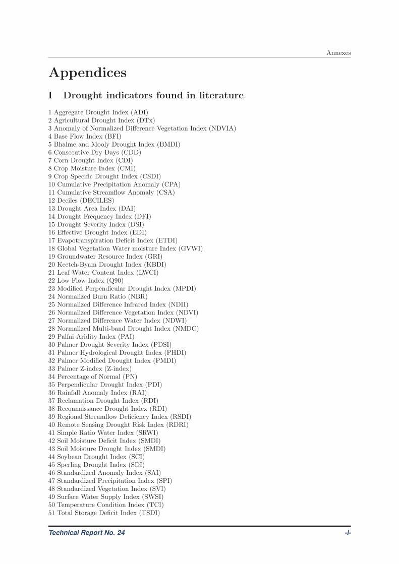
Annexes
Appendices
I Drought indicators found in literature
1 Aggregate Drought Index (ADI)2 Agricultural Drought Index (DTx)3 Anomaly of Normalized Difference Vegetation Index (NDVIA)4 Base Flow Index (BFI)5 Bhalme and Mooly Drought Index (BMDI)6 Consecutive Dry Days (CDD)7 Corn Drought Index (CDI)8 Crop Moisture Index (CMI)9 Crop Specific Drought Index (CSDI)10 Cumulative Precipitation Anomaly (CPA)11 Cumulative Streamflow Anomaly (CSA)12 Deciles (DECILES)13 Drought Area Index (DAI)14 Drought Frequency Index (DFI)15 Drought Severity Index (DSI)16 Effective Drought Index (EDI)17 Evapotranspiration Deficit Index (ETDI)18 Global Vegetation Water moisture Index (GVWI)19 Groundwater Resource Index (GRI)20 Keetch-Byam Drought Index (KBDI)21 Leaf Water Content Index (LWCI)22 Low Flow Index (Q90)23 Modified Perpendicular Drought Index (MPDI)24 Normalized Burn Ratio (NBR)25 Normalized Difference Infrared Index (NDII)26 Normalized Difference Vegetation Index (NDVI)27 Normalized Difference Water Index (NDWI)28 Normalized Multi-band Drought Index (NMDC)29 Palfai Aridity Index (PAI)30 Palmer Drought Severity Index (PDSI)31 Palmer Hydrological Drought Index (PHDI)32 Palmer Modified Drought Index (PMDI)33 Palmer Z-index (Z-index)34 Percentage of Normal (PN)35 Perpendicular Drought Index (PDI)36 Rainfall Anomaly Index (RAI)37 Reclamation Drought Index (RDI)38 Reconnaissance Drought Index (RDI)39 Regional Streamflow Deficiency Index (RSDI)40 Remote Sensing Drought Risk Index (RDRI)41 Simple Ratio Water Index (SRWI)42 Soil Moisture Deficit Index (SMDI)43 Soil Moisture Drought Index (SMDI)44 Soybean Drought Index (SCI)45 Sperling Drought Index (SDI)46 Standardized Anomaly Index (SAI)47 Standardized Precipitation Index (SPI)48 Standardized Vegetation Index (SVI)49 Surface Water Supply Index (SWSI)50 Temperature Condition Index (TCI)51 Total Storage Deficit Index (TSDI)
Technical Report No. 24 -i-
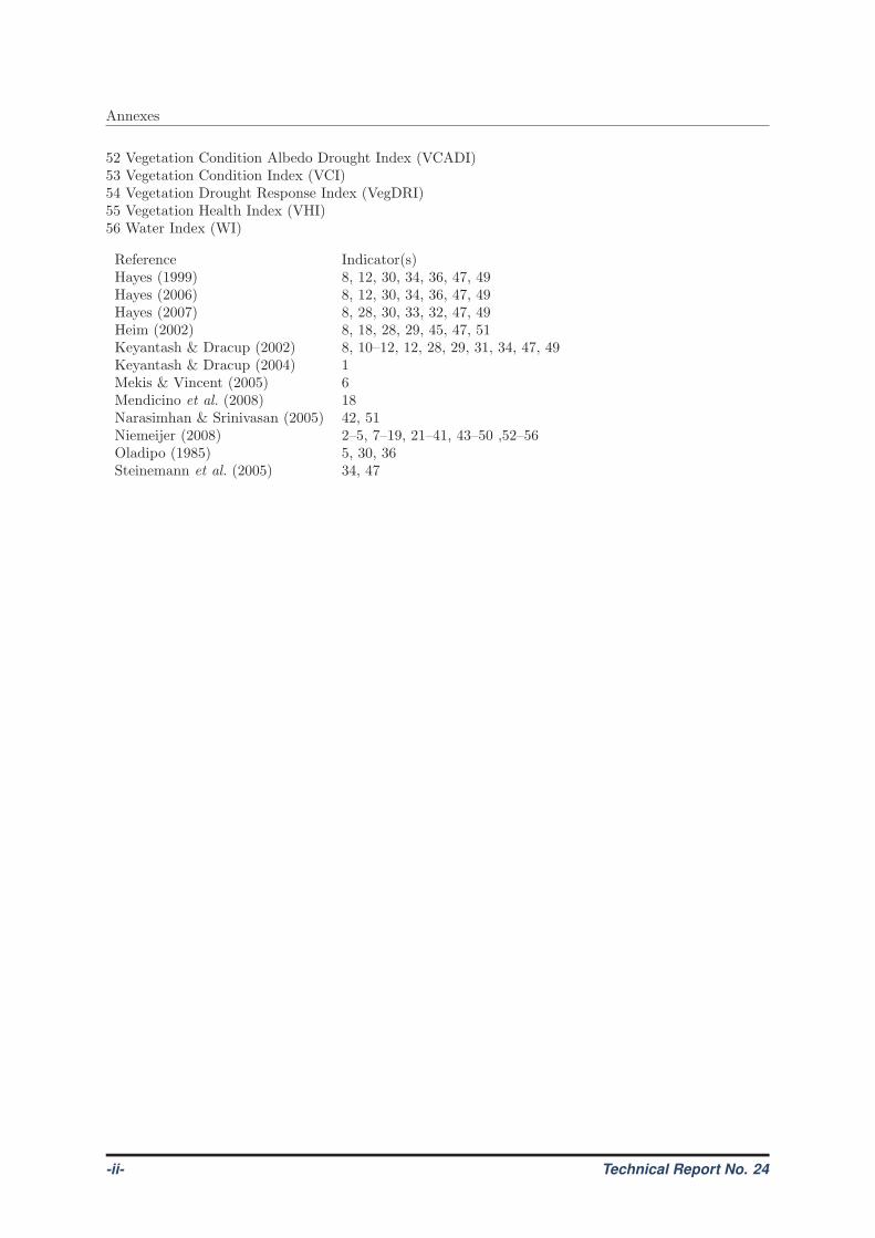
Annexes
52 Vegetation Condition Albedo Drought Index (VCADI)53 Vegetation Condition Index (VCI)54 Vegetation Drought Response Index (VegDRI)55 Vegetation Health Index (VHI)56 Water Index (WI)
Reference Indicator(s)Hayes (1999) 8, 12, 30, 34, 36, 47, 49Hayes (2006) 8, 12, 30, 34, 36, 47, 49Hayes (2007) 8, 28, 30, 33, 32, 47, 49Heim (2002) 8, 18, 28, 29, 45, 47, 51Keyantash & Dracup (2002) 8, 10–12, 12, 28, 29, 31, 34, 47, 49Keyantash & Dracup (2004) 1Mekis & Vincent (2005) 6Mendicino et al. (2008) 18Narasimhan & Srinivasan (2005) 42, 51Niemeijer (2008) 2–5, 7–19, 21–41, 43–50 ,52–56Oladipo (1985) 5, 30, 36Steinemann et al. (2005) 34, 47
-ii- Technical Report No. 24
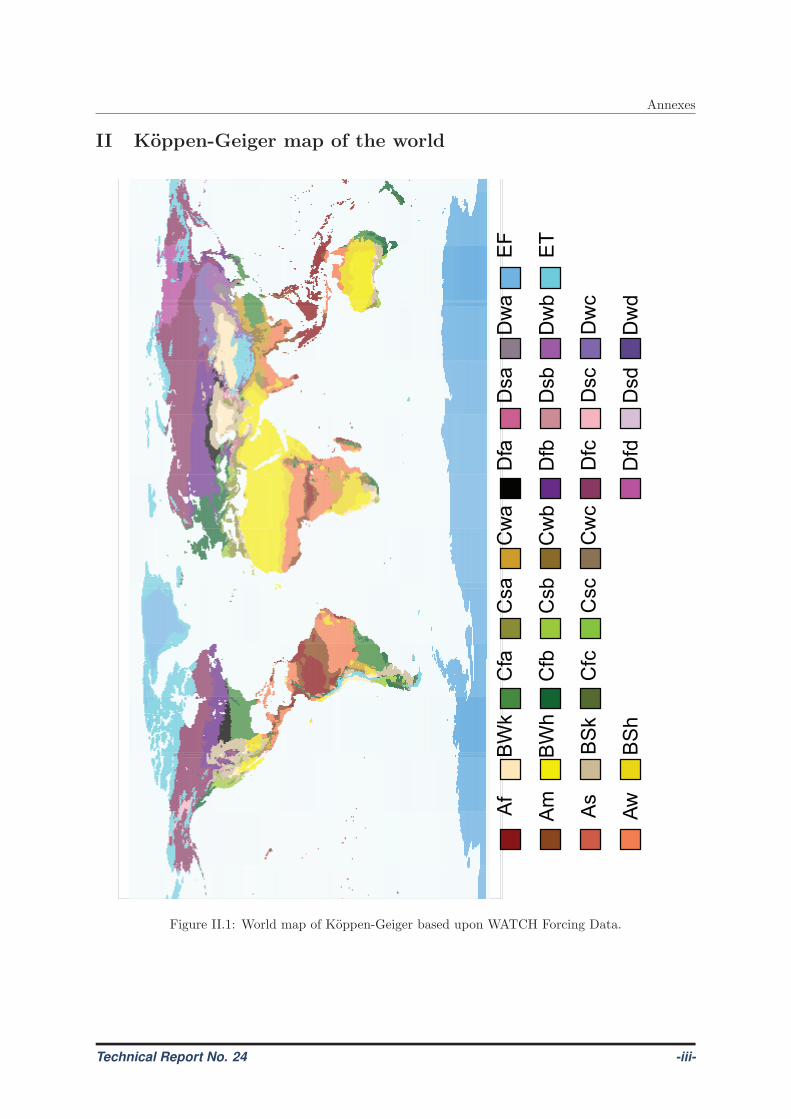
Annexes
II Koppen-Geiger map of the world
Af
Am
As
Aw
BW
k
BW
h
BS
k
BS
h
Cfa
Cfb
Cfc
Csa
Csb
Csc
Cw
a
Cw
b
Cw
c
Dfa
Dfb
Dfc
Dfd
Dsa
Dsb
Dsc
Dsd
Dw
a
Dw
b
Dw
c
Dw
d
EF
ET
Figure II.1: World map of Koppen-Geiger based upon WATCH Forcing Data.
Technical Report No. 24 -iii-

Annexes
-iv- Technical Report No. 24
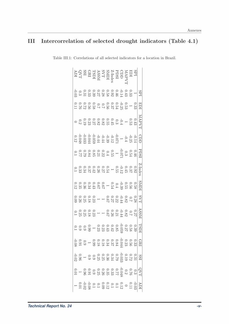
Annexes
III Intercorrelation of selected drought indicators (Table 4.1)
Table III.1: Correlations of all selected indicators for a location in Brazil.
SPI
EDI
MAPVT
CDD
PDSI
Z-Index
SMDI
SVT
ASSM
TSDI
GRI
SSI
QVT
ADI
SPI
10.33
0.43-0.14
0.460.92
0.580.28
0.270.39
0.33
0.310.3
-0.03EDI
0.331
0.53-0.25
0.540.37
0.560.7
0.70.5
80.56
0.72
0.760.11
MAPVT
0.430.53
1-0.4
0.30.45
0.550.82
0.820.27
0.230.19
0.20
CDD
-0.14-0.25
-0.41
-0.071-0.12
-0.39-0.44
-0.44-0.059
-0.044
-0.033
-0.048
0.12
PDSI
0.460.54
0.3-0.071
10.55
0.40.22
0.210.85
0.840.7
90.77
0.1Z-Index
0.920.37
0.45-0.12
0.551
0.540.27
0.260.42
0.370.34
0.33
0.1SMDI
0.580.56
0.55-0.39
0.40.54
10.67
0.670.4
30.34
0.36
0.350.12
SVT
0.280.7
0.82-0.44
0.220.27
0.671
10.23
0.180.25
0.260.09
ASSM
0.270.7
0.82-0.44
0.210.26
0.671
10.23
0.18
0.25
0.250.1
TSDI
0.390.58
0.27-0.059
0.850.42
0.430.23
0.231
0.99
0.90.9
0.1GRI
0.330.56
0.23-0.044
0.840.37
0.340.18
0.180.99
10.9
0.91-0.08
SSI
0.310.72
0.19-0.033
0.790.34
0.360.25
0.250.9
0.91
0.96
-0.02QVT
0.30.76
0.2-0.048
0.770.33
0.350.26
0.250.9
0.91
0.961
0.01
ADI
-0.030.11
00.12
0.10.1
0.120.09
0.10.1
-0.08-0.02
0.011
Technical Report No. 24 -v-
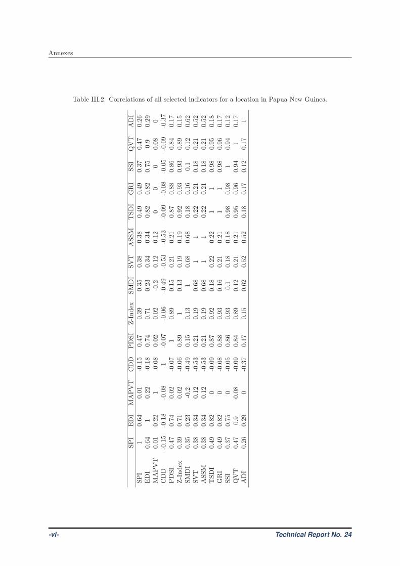
Annexes
Table III.2: Correlations of all selected indicators for a location in Papua New Guinea.
SPI
EDI
MAPVT
CDD
PDSI
Z-Index
SMDI
SVT
ASSM
TSDI
GRI
SSI
QVT
ADI
SPI
10.64
0.01
-0.15
0.47
0.39
0.35
0.38
0.38
0.49
0.49
0.37
0.47
0.26
EDI
0.64
10.22
-0.18
0.74
0.71
0.23
0.34
0.34
0.82
0.82
0.75
0.9
0.29
MAPVT
0.01
0.22
1-0.08
0.02
0.02
-0.2
0.12
0.12
00
00.08
0CDD
-0.15
-0.18
-0.08
1-0.07
-0.06
-0.49
-0.53
-0.53
-0.09
-0.08
-0.05
-0.09
-0.37
PDSI
0.47
0.74
0.02
-0.07
10.89
0.15
0.21
0.21
0.87
0.88
0.86
0.84
0.17
Z-Index
0.39
0.71
0.02
-0.06
0.89
10.13
0.19
0.19
0.92
0.93
0.93
0.89
0.15
SMDI
0.35
0.23
-0.2
-0.49
0.15
0.13
10.68
0.68
0.18
0.16
0.1
0.12
0.62
SVT
0.38
0.34
0.12
-0.53
0.21
0.19
0.68
11
0.22
0.21
0.18
0.21
0.52
ASSM
0.38
0.34
0.12
-0.53
0.21
0.19
0.68
11
0.22
0.21
0.18
0.21
0.52
TSDI
0.49
0.82
0-0.09
0.87
0.92
0.18
0.22
0.22
11
0.98
0.95
0.18
GRI
0.49
0.82
0-0.08
0.88
0.93
0.16
0.21
0.21
11
0.98
0.96
0.17
SSI
0.37
0.75
0-0.05
0.86
0.93
0.1
0.18
0.18
0.98
0.98
10.94
0.12
QVT
0.47
0.9
0.08
-0.09
0.84
0.89
0.12
0.21
0.21
0.95
0.96
0.94
10.17
ADI
0.26
0.29
0-0.37
0.17
0.15
0.62
0.52
0.52
0.18
0.17
0.12
0.17
1
-vi- Technical Report No. 24
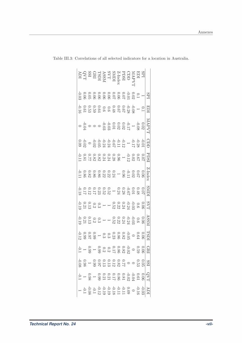
Annexes
Table III.3: Correlations of all selected indicators for a location in Australia.
SPI
EDI
MAPVT
CDD
PDSI
Z-Index
SMDI
SVT
ASSM
TSDI
GRI
SSI
QVT
ADI
SPI
10.1
0.02-0.01
0.070.06
0.070.06
0.060.06
0.060.05
0.06
-0.03EDI
0.11
-0.08-0.28
0.670.67
0.480.6
0.60.64
0.590.53
0.61
-0.16MAPVT
0.02-0.08
1-0.17
0.020.02
0.01-0.03
-0.030
00
-0.040
CDD
-0.01-0.28
-0.171
-0.12-0.11
-0.67-0.24
-0.24-0.05
-0.02
0-0.02
0.09PDSI
0.070.67
0.02-0.12
10.96
0.280.24
0.24
0.820.82
0.77
0.81
-0.11Z-Index
0.060.67
0.02-0.11
0.961
0.240.22
0.220.86
0.860.82
0.86-0.1
1SMDI
0.070.48
0.01-0.67
0.280.24
10.52
0.520.23
0.170.12
0.17-0.18
SVT
0.060.6
-0.03-0.24
0.240.22
0.521
10.3
0.20.13
0.21
-0.19ASSM
0.060.6
-0.03-0.24
0.240.22
0.521
10.3
0.20.13
0.21-0.19
TSDI
0.060.64
0-0.05
0.820.86
0.230.3
0.31
0.99
0.970.9
9-0.12
GRI
0.060.59
0-0.02
0.820.86
0.170.2
0.20.99
10.99
1-0.1
SSI
0.050.53
00
0.770.82
0.120.13
0.13
0.970.99
10.98
-0.08QVT
0.060.61
-0.04-0.02
0.810.86
0.170.21
0.210.99
10.98
1-0.1
ADI
-0.03-0.16
00.09
-0.11-0.11
-0.18-0.19
-0.19-0.12
-0.1-0.0
8-0.1
1
Technical Report No. 24 -vii-
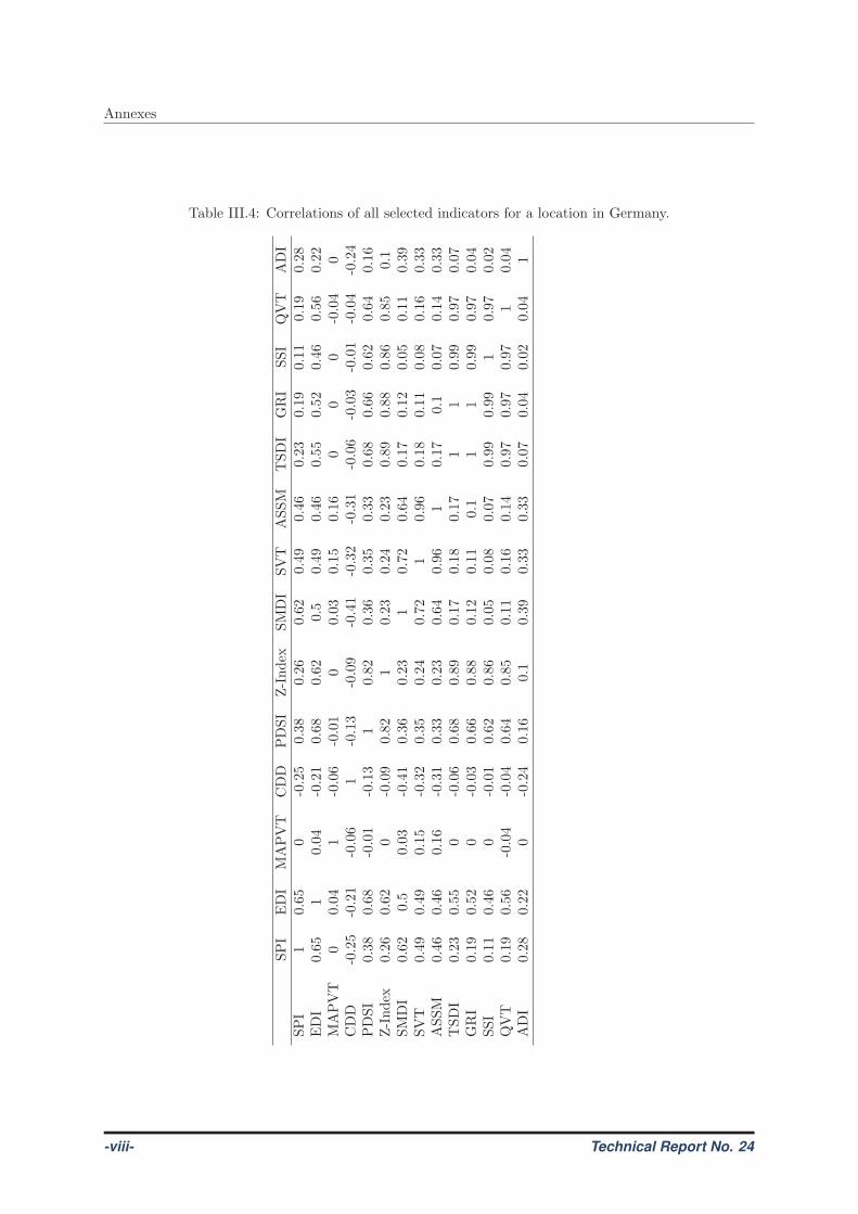
Annexes
Table III.4: Correlations of all selected indicators for a location in Germany.
SPI
EDI
MAPVT
CDD
PDSI
Z-Index
SMDI
SVT
ASSM
TSDI
GRI
SSI
QVT
ADI
SPI
10.65
0-0.25
0.38
0.26
0.62
0.49
0.46
0.23
0.19
0.11
0.19
0.28
EDI
0.65
10.04
-0.21
0.68
0.62
0.5
0.49
0.46
0.55
0.52
0.46
0.56
0.22
MAPVT
00.04
1-0.06
-0.01
00.03
0.15
0.16
00
0-0.04
0CDD
-0.25
-0.21
-0.06
1-0.13
-0.09
-0.41
-0.32
-0.31
-0.06
-0.03
-0.01
-0.04
-0.24
PDSI
0.38
0.68
-0.01
-0.13
10.82
0.36
0.35
0.33
0.68
0.66
0.62
0.64
0.16
Z-Index
0.26
0.62
0-0.09
0.82
10.23
0.24
0.23
0.89
0.88
0.86
0.85
0.1
SMDI
0.62
0.5
0.03
-0.41
0.36
0.23
10.72
0.64
0.17
0.12
0.05
0.11
0.39
SVT
0.49
0.49
0.15
-0.32
0.35
0.24
0.72
10.96
0.18
0.11
0.08
0.16
0.33
ASSM
0.46
0.46
0.16
-0.31
0.33
0.23
0.64
0.96
10.17
0.1
0.07
0.14
0.33
TSDI
0.23
0.55
0-0.06
0.68
0.89
0.17
0.18
0.17
11
0.99
0.97
0.07
GRI
0.19
0.52
0-0.03
0.66
0.88
0.12
0.11
0.1
11
0.99
0.97
0.04
SSI
0.11
0.46
0-0.01
0.62
0.86
0.05
0.08
0.07
0.99
0.99
10.97
0.02
QVT
0.19
0.56
-0.04
-0.04
0.64
0.85
0.11
0.16
0.14
0.97
0.97
0.97
10.04
ADI
0.28
0.22
0-0.24
0.16
0.1
0.39
0.33
0.33
0.07
0.04
0.02
0.04
1
-viii- Technical Report No. 24
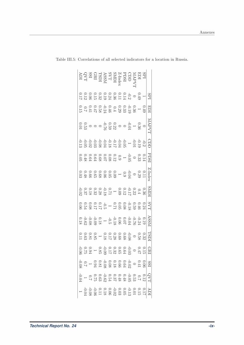
Annexes
Table III.5: Correlations of all selected indicators for a location in Russia.
SPI
EDI
MAPVT
CDD
PDSI
Z-Index
SMDI
SVT
ASSM
TSDI
GRI
SSI
QVT
ADI
SPI
10.49
0-0.2
0.140.11
0.360.24
0.190.32
0.150.0
60.12
0.17EDI
0.491
0.36-0.19
0.330.29
0.40.46
-0.240.58
0.470.41
0.70.15
MAPVT
00.36
1-0.01
00
0.220.59
-0.760
00
0.530.01
CDD
-0.2-0.19
-0.011
-0.05-0.04
-0.17-0.18
-0.04-0.08
-0.03-0.02
-0.05
-0.13PDSI
0.140.33
0-0.05
10.9
0.120.08
0.070.68
0.640.64
0.48
0.05Z-Index
0.110.29
0-0.04
0.91
0.090.05
0.060.68
0.65
0.66
0.480.03
SMDI
0.360.4
0.22-0.17
0.120.09
10.71
-0.180.28
0.320.18
0.37
-0.02SVT
0.240.46
0.59-0.18
0.080.05
0.711
-0.50.17
0.17
0.08
0.54
0.06ASSM
0.19-0.24
-0.76-0.04
0.070.06
-0.18-0.5
10.18
-0.09
-0.08
-0.62
0.18
TSDI
0.320.58
0-0.08
0.680.68
0.280.17
0.181
0.850.81
0.630.11
GRI
0.150.47
0-0.03
0.640.65
0.320.17
-0.090.85
10.94
0.75
-0.06SSI
0.060.41
0-0.02
0.640.66
0.180.08
-0.080.81
0.941
0.7-0.08
QVT
0.120.7
0.53-0.05
0.480.48
0.370.54
-0.620.63
0.750.7
1-0.04
ADI
0.170.15
0.01-0.13
0.050.03
-0.020.06
0.180.11
-0.06-0.08
-0.041
Technical Report No. 24 -ix-
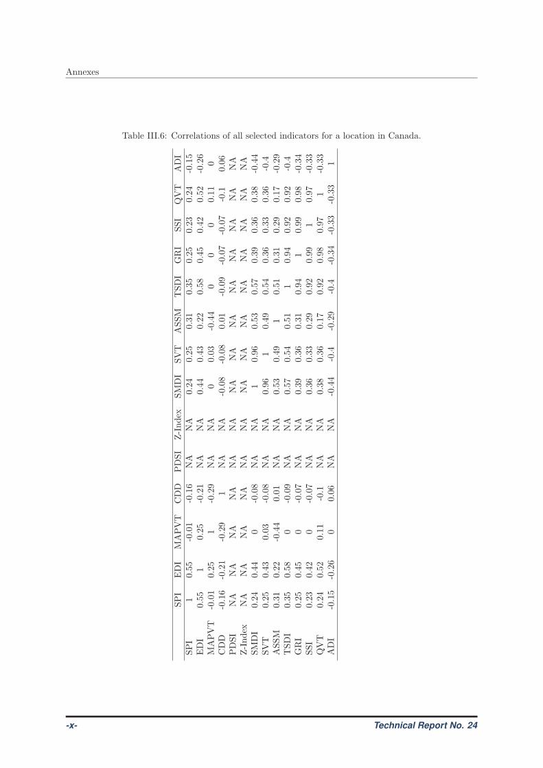
Annexes
Table III.6: Correlations of all selected indicators for a location in Canada.
SPI
EDI
MAPVT
CDD
PDSI
Z-Index
SMDI
SVT
ASSM
TSDI
GRI
SSI
QVT
ADI
SPI
10.55
-0.01
-0.16
NA
NA
0.24
0.25
0.31
0.35
0.25
0.23
0.24
-0.15
EDI
0.55
10.25
-0.21
NA
NA
0.44
0.43
0.22
0.58
0.45
0.42
0.52
-0.26
MAPVT
-0.01
0.25
1-0.29
NA
NA
00.03
-0.44
00
00.11
0CDD
-0.16
-0.21
-0.29
1NA
NA
-0.08
-0.08
0.01
-0.09
-0.07
-0.07
-0.1
0.06
PDSI
NA
NA
NA
NA
NA
NA
NA
NA
NA
NA
NA
NA
NA
NA
Z-Index
NA
NA
NA
NA
NA
NA
NA
NA
NA
NA
NA
NA
NA
NA
SMDI
0.24
0.44
0-0.08
NA
NA
10.96
0.53
0.57
0.39
0.36
0.38
-0.44
SVT
0.25
0.43
0.03
-0.08
NA
NA
0.96
10.49
0.54
0.36
0.33
0.36
-0.4
ASSM
0.31
0.22
-0.44
0.01
NA
NA
0.53
0.49
10.51
0.31
0.29
0.17
-0.29
TSDI
0.35
0.58
0-0.09
NA
NA
0.57
0.54
0.51
10.94
0.92
0.92
-0.4
GRI
0.25
0.45
0-0.07
NA
NA
0.39
0.36
0.31
0.94
10.99
0.98
-0.34
SSI
0.23
0.42
0-0.07
NA
NA
0.36
0.33
0.29
0.92
0.99
10.97
-0.33
QVT
0.24
0.52
0.11
-0.1
NA
NA
0.38
0.36
0.17
0.92
0.98
0.97
1-0.33
ADI
-0.15
-0.26
00.06
NA
NA
-0.44
-0.4
-0.29
-0.4
-0.34
-0.33
-0.33
1
-x- Technical Report No. 24
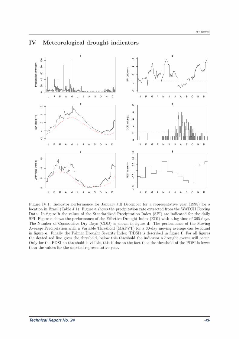
Annexes
IV Meteorological drought indicators
a
Pre
cip
itation (
mm
/day)
020
40
60
80
100
J F M A M J J A S O N D
b
SP
I valu
e (
−)
−2
−1
01
2
J F M A M J J A S O N D
c
ED
I valu
e (
−)
−2
−1
01
2
J F M A M J J A S O N D
d
CC
D v
alu
e (
d)
02
46
810
J F M A M J J A S O N D
e
MA
P v
alu
e (
mm
/d)
05
10
15
J F M A M J J A S O N D
f
PD
SI valu
e (
−)
−1.5
−0.5
0.5
1.0
1.5
J F M A M J J A S O N D
Figure IV.1: Indicator performance for January till December for a representative year (1995) for alocation in Brasil (Table 4.1). Figure a shows the precipitation rate extracted from the WATCH ForcingData. In figure b the values of the Standardized Precipitation Index (SPI) are indicated for the dailySPI. Figure c shows the performance of the Effective Drought Index (EDI) with a lag time of 365 days.The Number of Consecutive Dry Days (CDD) is shown in figure d. The performance of the MovingAverage Precipitation with a Variable Threshold (MAPVT) for a 30-day moving average can be foundin figure e. Finally the Palmer Drought Severity Index (PDSI) is described in figure f. For all figuresthe dotted red line gives the threshold, below this threshold the indicator a drought events will occur.Only for the PDSI no threshold is visible, this is due to the fact that the threshold of the PDSI is lowerthan the values for the selected representative year.
Technical Report No. 24 -xi-
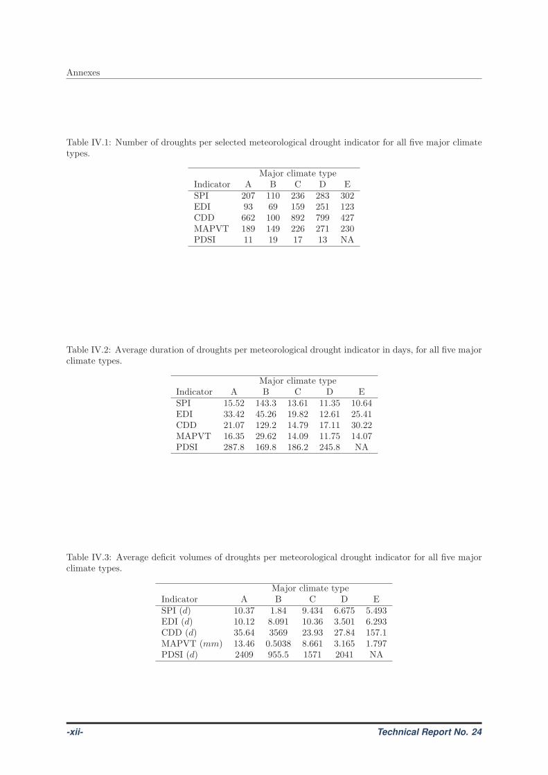
Annexes
Table IV.1: Number of droughts per selected meteorological drought indicator for all five major climatetypes.
Major climate typeIndicator A B C D ESPI 207 110 236 283 302EDI 93 69 159 251 123CDD 662 100 892 799 427MAPVT 189 149 226 271 230PDSI 11 19 17 13 NA
Table IV.2: Average duration of droughts per meteorological drought indicator in days, for all five majorclimate types.
Major climate typeIndicator A B C D ESPI 15.52 143.3 13.61 11.35 10.64EDI 33.42 45.26 19.82 12.61 25.41CDD 21.07 129.2 14.79 17.11 30.22MAPVT 16.35 29.62 14.09 11.75 14.07PDSI 287.8 169.8 186.2 245.8 NA
Table IV.3: Average deficit volumes of droughts per meteorological drought indicator for all five majorclimate types.
Major climate typeIndicator A B C D ESPI (d) 10.37 1.84 9.434 6.675 5.493EDI (d) 10.12 8.091 10.36 3.501 6.293CDD (d) 35.64 3569 23.93 27.84 157.1MAPVT (mm) 13.46 0.5038 8.661 3.165 1.797PDSI (d) 2409 955.5 1571 2041 NA
-xii- Technical Report No. 24
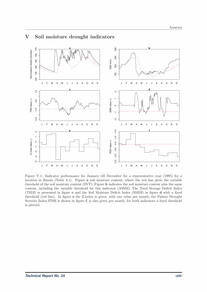
Annexes
V Soil moisture drought indicators
a
Soil
mois
ture
conte
nt (m
m/d
ay)
120
130
140
150
160
170
J F M A M J J A S O N D
b
SS
M (
mm
)
150
200
250
300
J F M A M J J A S O N D
c
TS
DI valu
e (
−)
−2.0
−1.0
0.0
1.0
J F M A M J J A S O N D
d
SM
DI valu
e (
−)
−2
−1
01
2
J F M A M J J A S O N D
e
Z−
index v
alu
e (
−)
−4
−3
−2
−1
01
2
J F M A M J J A S O N D
f
PD
SI valu
e (
−)
−3.5
−3.0
−2.5
−2.0
−1.5
−1.0
J F M A M J J A S O N D
Figure V.1: Indicator performance for January till December for a representative year (1995) for alocation in Russia (Table 4.1). Figure a soil moisture content, where the red line gives the variablethreshold of the soil moisture content (SVT). Figure b indicates the soil moisture content plus the snowcontent, including the variable threshold for this indicator (ASSM). The Total Storage Deficit Index(TSDI) is presented in figure c and the Soil Moisture Deficit Index (SMDI) in figure d with a fixedthreshold (red line). In figure e the Z-index is given, with one value per month, the Palmer DroughtSeverity Index PDSI is shown in figure f, is also given per month, for both indicators a fixed thresholdis plotted.
Technical Report No. 24 -xiii-
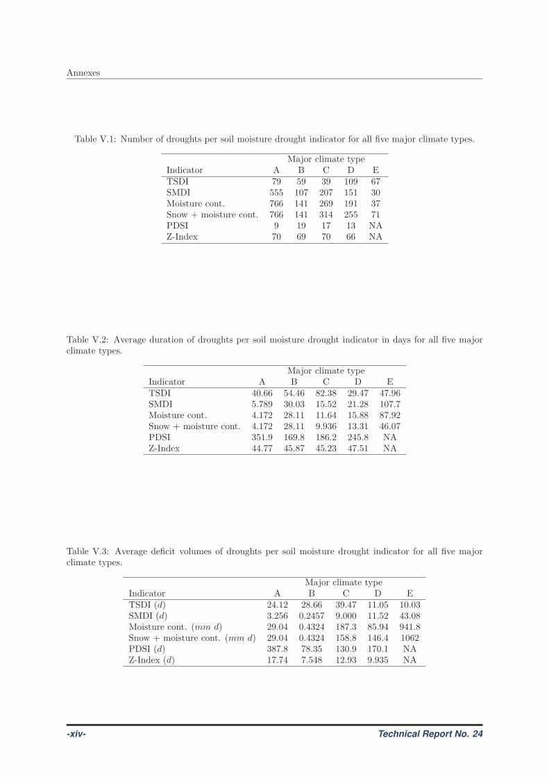
Annexes
Table V.1: Number of droughts per soil moisture drought indicator for all five major climate types.
Major climate typeIndicator A B C D ETSDI 79 59 39 109 67SMDI 555 107 207 151 30Moisture cont. 766 141 269 191 37Snow + moisture cont. 766 141 314 255 71PDSI 9 19 17 13 NAZ-Index 70 69 70 66 NA
Table V.2: Average duration of droughts per soil moisture drought indicator in days for all five majorclimate types.
Major climate typeIndicator A B C D ETSDI 40.66 54.46 82.38 29.47 47.96SMDI 5.789 30.03 15.52 21.28 107.7Moisture cont. 4.172 28.11 11.64 15.88 87.92Snow + moisture cont. 4.172 28.11 9.936 13.31 46.07PDSI 351.9 169.8 186.2 245.8 NAZ-Index 44.77 45.87 45.23 47.51 NA
Table V.3: Average deficit volumes of droughts per soil moisture drought indicator for all five majorclimate types.
Major climate typeIndicator A B C D ETSDI (d) 24.12 28.66 39.47 11.05 10.03SMDI (d) 3.256 0.2457 9.000 11.52 43.08Moisture cont. (mm d) 29.04 0.4324 187.3 85.94 941.8Snow + moisture cont. (mm d) 29.04 0.4324 158.8 146.4 1062PDSI (d) 387.8 78.35 130.9 170.1 NAZ-Index (d) 17.74 7.548 12.93 9.935 NA
-xiv- Technical Report No. 24
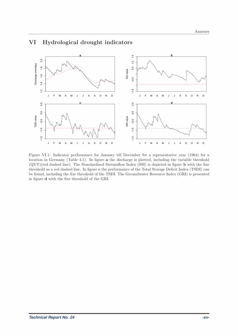
Annexes
VI Hydrological drought indicators
a
Dis
charg
e (
mm
/day)
1.2
1.4
1.6
1.8
2.0
J F M A M J J A S O N D
b
SS
I valu
e
−1.5
−0.5
0.5
1.0
1.5
J F M A M J J A S O N D
c
TS
DI valu
e
−1.5
−1.0
−0.5
0.0
0.5
J F M A M J J A S O N D
d
GR
I valu
e
−1.5
−1.0
−0.5
0.0
0.5
J F M A M J J A S O N D
Figure VI.1: Indicator performance for January till December for a representative year (1964) for alocation in Germany (Table 4.1). In figure a the discharge is plotted, including the variable threshold(QVT)(red dashed line). The Standardized Streamflow Index (SSI) is depicted in figure b with the fixethreshold as a red dashed line. In figure c the performance of the Total Storage Deficit Index (TSDI) canbe found, including the fixe threshold of the TSDI. The Groundwater Resource Index (GRI) is presentedin figure d with the fixe threshold of the GRI.
Technical Report No. 24 -xv-
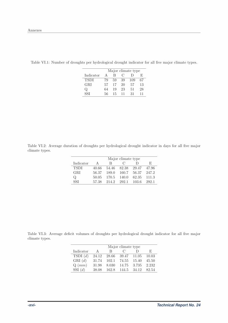
Annexes
Table VI.1: Number of droughts per hydrological drought indicator for all five major climate types.
Major climate typeIndicator A B C D ETSDI 79 59 39 109 67GRI 57 17 20 57 13Q 64 19 23 51 28SSI 56 15 11 31 11
Table VI.2: Average duration of droughts per hydrological drought indicator in days for all five majorclimate types.
Major climate typeIndicator A B C D ETSDI 40.66 54.46 82.38 29.47 47.96GRI 56.37 189.0 160.7 56.37 247.2Q 50.05 170.5 140.0 62.35 111.3SSI 57.38 214.2 292.1 103.6 292.1
Table VI.3: Average deficit volumes of droughts per hydrological drought indicator for all five majorclimate types.
Major climate typeIndicator A B C D ETSDI (d) 24.12 28.66 39.47 11.05 10.03GRI (d) 31.74 102.1 74.55 15.40 45.50Q (mm) 31.98 8.030 14.75 3.735 2.232SSI (d) 38.08 162.8 144.5 34.12 82.54
-xvi- Technical Report No. 24
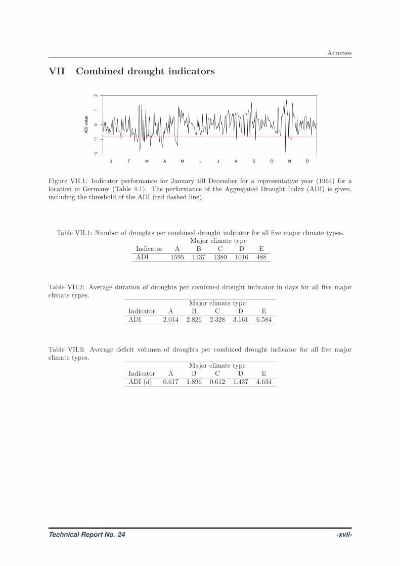
Annexes
VII Combined drought indicators
AD
I valu
e
−2
−1
01
2
J F M A M J J A S O N D
Figure VII.1: Indicator performance for January till December for a representative year (1964) for alocation in Germany (Table 4.1). The performance of the Aggregated Drought Index (ADI) is given,including the threshold of the ADI (red dashed line).
Table VII.1: Number of droughts per combined drought indicator for all five major climate types.Major climate type
Indicator A B C D EADI 1595 1137 1380 1016 488
Table VII.2: Average duration of droughts per combined drought indicator in days for all five majorclimate types.
Major climate typeIndicator A B C D EADI 2.014 2.826 2.328 3.161 6.584
Table VII.3: Average deficit volumes of droughts per combined drought indicator for all five majorclimate types.
Major climate typeIndicator A B C D EADI (d) 0.617 1.896 0.612 1.437 4.634
Technical Report No. 24 -xvii-

Annexes
-xviii- Technical Report No. 24
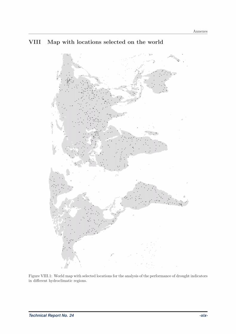
Annexes
VIII Map with locations selected on the world
Figure VIII.1: World map with selected locations for the analysis of the performance of drought indicatorsin different hydroclimatic regions.
Technical Report No. 24 -xix-

Annexes
-xx- Technical Report No. 24
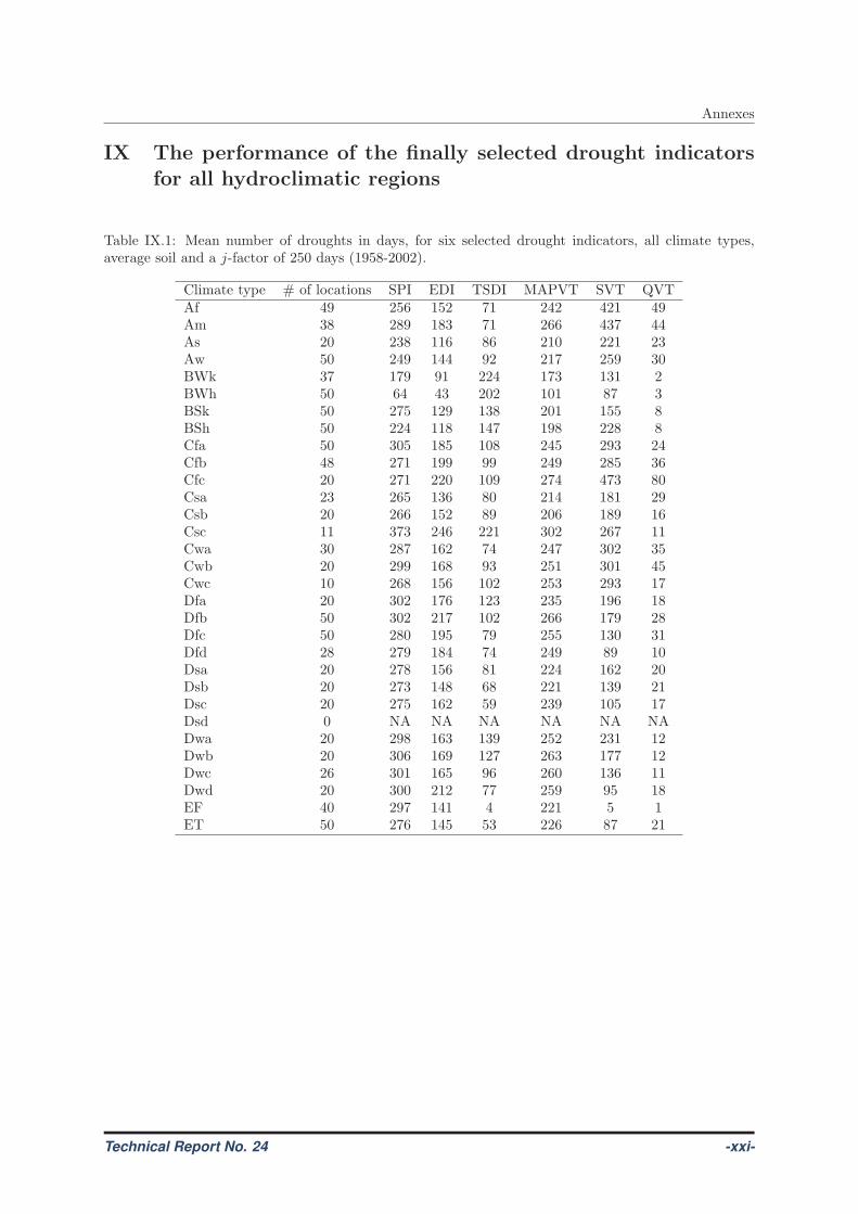
Annexes
IX The performance of the finally selected drought indicatorsfor all hydroclimatic regions
Table IX.1: Mean number of droughts in days, for six selected drought indicators, all climate types,average soil and a j-factor of 250 days (1958-2002).
Climate type # of locations SPI EDI TSDI MAPVT SVT QVTAf 49 256 152 71 242 421 49Am 38 289 183 71 266 437 44As 20 238 116 86 210 221 23Aw 50 249 144 92 217 259 30BWk 37 179 91 224 173 131 2BWh 50 64 43 202 101 87 3BSk 50 275 129 138 201 155 8BSh 50 224 118 147 198 228 8Cfa 50 305 185 108 245 293 24Cfb 48 271 199 99 249 285 36Cfc 20 271 220 109 274 473 80Csa 23 265 136 80 214 181 29Csb 20 266 152 89 206 189 16Csc 11 373 246 221 302 267 11Cwa 30 287 162 74 247 302 35Cwb 20 299 168 93 251 301 45Cwc 10 268 156 102 253 293 17Dfa 20 302 176 123 235 196 18Dfb 50 302 217 102 266 179 28Dfc 50 280 195 79 255 130 31Dfd 28 279 184 74 249 89 10Dsa 20 278 156 81 224 162 20Dsb 20 273 148 68 221 139 21Dsc 20 275 162 59 239 105 17Dsd 0 NA NA NA NA NA NADwa 20 298 163 139 252 231 12Dwb 20 306 169 127 263 177 12Dwc 26 301 165 96 260 136 11Dwd 20 300 212 77 259 95 18EF 40 297 141 4 221 5 1ET 50 276 145 53 226 87 21
Technical Report No. 24 -xxi-
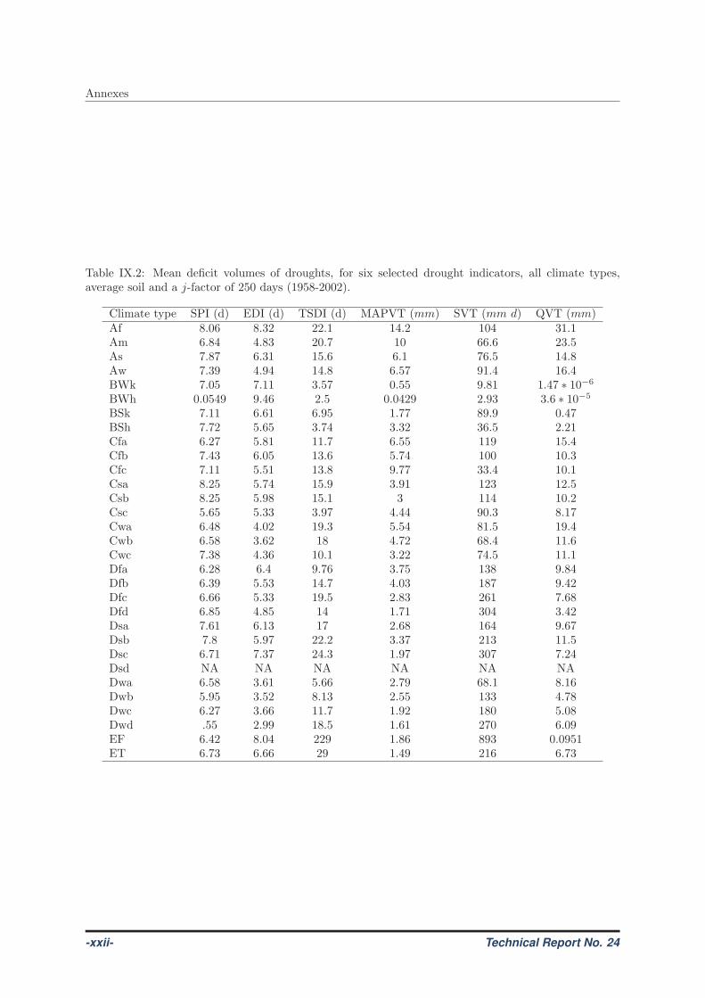
Annexes
Table IX.2: Mean deficit volumes of droughts, for six selected drought indicators, all climate types,average soil and a j-factor of 250 days (1958-2002).
Climate type SPI (d) EDI (d) TSDI (d) MAPVT (mm) SVT (mm d) QVT (mm)Af 8.06 8.32 22.1 14.2 104 31.1Am 6.84 4.83 20.7 10 66.6 23.5As 7.87 6.31 15.6 6.1 76.5 14.8Aw 7.39 4.94 14.8 6.57 91.4 16.4BWk 7.05 7.11 3.57 0.55 9.81 1.47 ∗ 10−6
BWh 0.0549 9.46 2.5 0.0429 2.93 3.6 ∗ 10−5
BSk 7.11 6.61 6.95 1.77 89.9 0.47BSh 7.72 5.65 3.74 3.32 36.5 2.21Cfa 6.27 5.81 11.7 6.55 119 15.4Cfb 7.43 6.05 13.6 5.74 100 10.3Cfc 7.11 5.51 13.8 9.77 33.4 10.1Csa 8.25 5.74 15.9 3.91 123 12.5Csb 8.25 5.98 15.1 3 114 10.2Csc 5.65 5.33 3.97 4.44 90.3 8.17Cwa 6.48 4.02 19.3 5.54 81.5 19.4Cwb 6.58 3.62 18 4.72 68.4 11.6Cwc 7.38 4.36 10.1 3.22 74.5 11.1Dfa 6.28 6.4 9.76 3.75 138 9.84Dfb 6.39 5.53 14.7 4.03 187 9.42Dfc 6.66 5.33 19.5 2.83 261 7.68Dfd 6.85 4.85 14 1.71 304 3.42Dsa 7.61 6.13 17 2.68 164 9.67Dsb 7.8 5.97 22.2 3.37 213 11.5Dsc 6.71 7.37 24.3 1.97 307 7.24Dsd NA NA NA NA NA NADwa 6.58 3.61 5.66 2.79 68.1 8.16Dwb 5.95 3.52 8.13 2.55 133 4.78Dwc 6.27 3.66 11.7 1.92 180 5.08Dwd .55 2.99 18.5 1.61 270 6.09EF 6.42 8.04 229 1.86 893 0.0951ET 6.73 6.66 29 1.49 216 6.73
-xxii- Technical Report No. 24
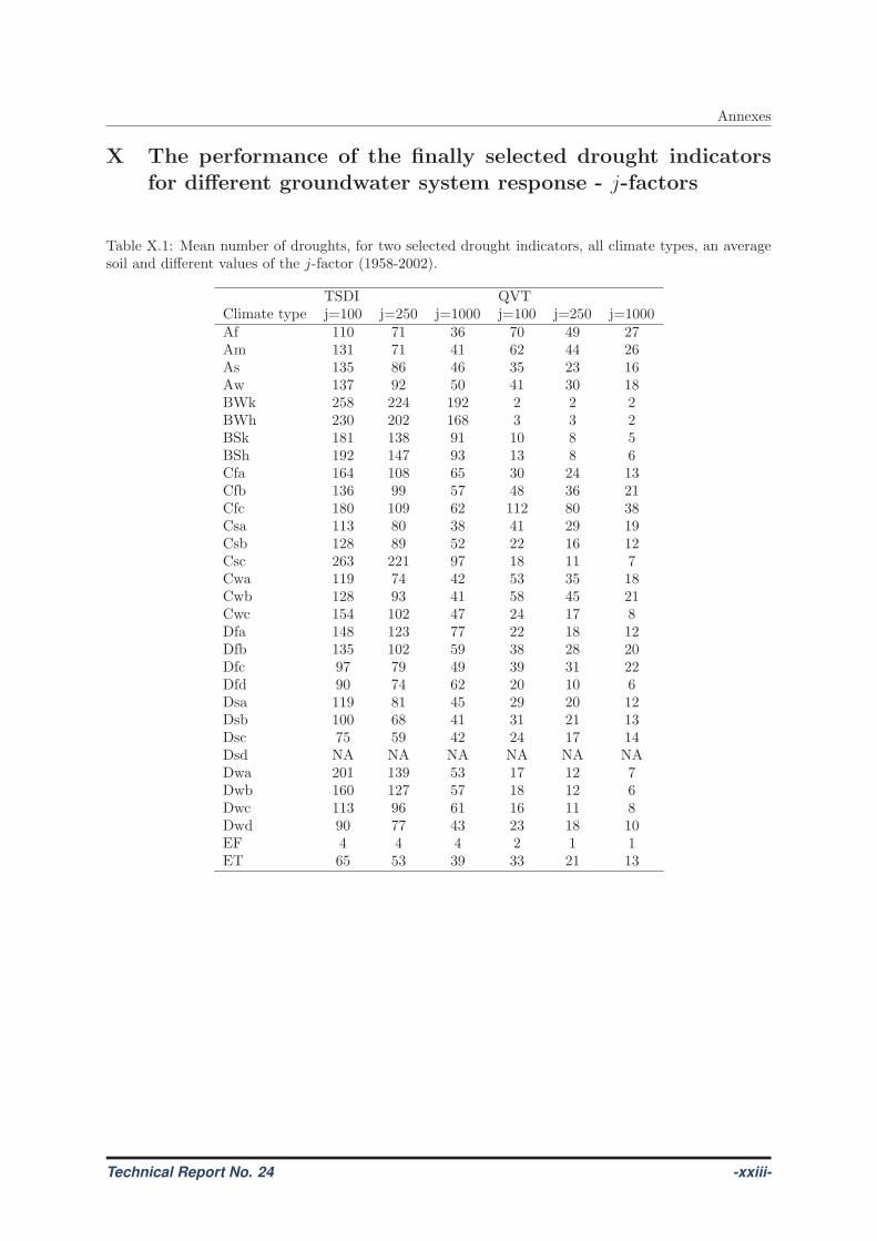
Annexes
X The performance of the finally selected drought indicatorsfor different groundwater system response - j-factors
Table X.1: Mean number of droughts, for two selected drought indicators, all climate types, an averagesoil and different values of the j-factor (1958-2002).
TSDI QVTClimate type j=100 j=250 j=1000 j=100 j=250 j=1000Af 110 71 36 70 49 27Am 131 71 41 62 44 26As 135 86 46 35 23 16Aw 137 92 50 41 30 18BWk 258 224 192 2 2 2BWh 230 202 168 3 3 2BSk 181 138 91 10 8 5BSh 192 147 93 13 8 6Cfa 164 108 65 30 24 13Cfb 136 99 57 48 36 21Cfc 180 109 62 112 80 38Csa 113 80 38 41 29 19Csb 128 89 52 22 16 12Csc 263 221 97 18 11 7Cwa 119 74 42 53 35 18Cwb 128 93 41 58 45 21Cwc 154 102 47 24 17 8Dfa 148 123 77 22 18 12Dfb 135 102 59 38 28 20Dfc 97 79 49 39 31 22Dfd 90 74 62 20 10 6Dsa 119 81 45 29 20 12Dsb 100 68 41 31 21 13Dsc 75 59 42 24 17 14Dsd NA NA NA NA NA NADwa 201 139 53 17 12 7Dwb 160 127 57 18 12 6Dwc 113 96 61 16 11 8Dwd 90 77 43 23 18 10EF 4 4 4 2 1 1ET 65 53 39 33 21 13
Technical Report No. 24 -xxiii-
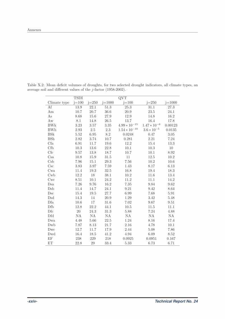
Annexes
Table X.2: Mean deficit volumes of droughts, for two selected drought indicators, all climate types, anaverage soil and different values of the j-factor (1958-2002).
TSDI QVTClimate type j=100 j=250 j=1000 j=100 j=250 j=1000Af 13.9 22.1 51.3 25.3 31.1 27.3Am 10.7 20.7 36.6 20.9 23.5 24.1As 8.68 15.6 27.9 12.9 14.8 16.2Aw 8.1 14.8 26.5 13.7 16.4 17.8BWk 3.23 3.57 3.35 4.99 ∗ 10−15 1.47 ∗ 10−6 0.00123BWh 2.93 2.5 2.3 1.54 ∗ 10−10 3.6 ∗ 10−5 0.0135BSk 5.52 6.95 8.2 0.0248 0.47 3.05BSh 2.82 3.74 10.7 0.281 2.21 7.24Cfa 6.91 11.7 19.6 12.2 15.4 13.3Cfb 10.3 13.6 22.8 10.1 10.3 10Cfc 9.57 13.8 18.7 10.7 10.1 8.92Csa 10.8 15.9 31.5 11 12.5 10.2Csb 7.96 15.1 29.3 7.56 10.2 10.6Csc 3.83 3.97 7.59 1.43 8.17 6.13Cwa 11.4 19.3 32.5 16.8 19.4 18.3Cwb 12.2 18 38.1 10.2 11.6 13.4Cwc 8.51 10.1 24.2 11.2 11.1 14.2Dsa 7.26 9.76 16.2 7.35 9.84 9.62Dsb 11.4 14.7 24.1 9.21 9.42 8.64Dsc 15.4 19.5 27.7 6.99 7.68 5.91Dsd 14.3 14 20.9 1.29 3.42 5.48Dfa 10.6 17 31.6 7.02 9.67 9.51Dfb 12.8 22.2 44.1 10.5 11.5 11.1Dfc 20 24.3 31.3 5.88 7.24 4.88Dfd NA NA NA NA NA NADwa 4.48 5.66 22.5 1.24 8.16 17.4Dwb 7.87 8.13 21.7 2.16 4.78 10.1Dwc 12.7 11.7 17.9 2.44 5.08 7.86Dwd 16.4 18.5 41.2 4.94 6.09 8.52EF 238 229 218 0.0925 0.0951 0.167ET 22.8 29 33.4 5.33 6.73 6.71
-xxiv- Technical Report No. 24
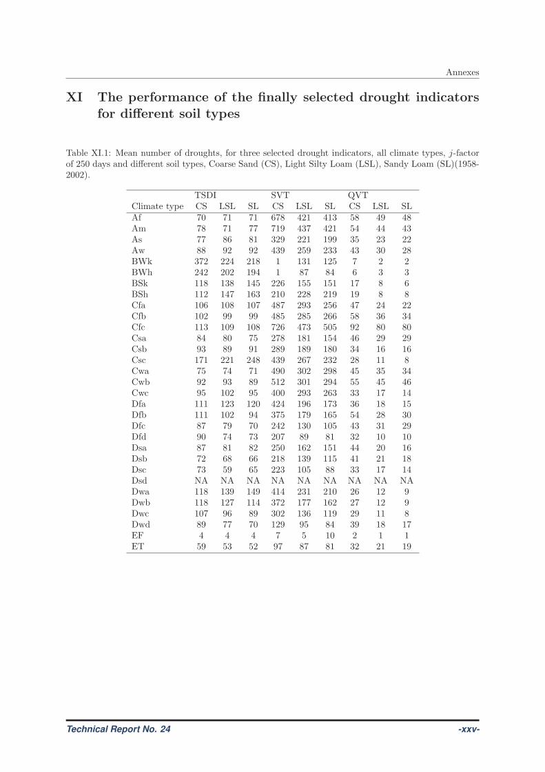
Annexes
XI The performance of the finally selected drought indicatorsfor different soil types
Table XI.1: Mean number of droughts, for three selected drought indicators, all climate types, j-factorof 250 days and different soil types, Coarse Sand (CS), Light Silty Loam (LSL), Sandy Loam (SL)(1958-2002).
TSDI SVT QVTClimate type CS LSL SL CS LSL SL CS LSL SLAf 70 71 71 678 421 413 58 49 48Am 78 71 77 719 437 421 54 44 43As 77 86 81 329 221 199 35 23 22Aw 88 92 92 439 259 233 43 30 28BWk 372 224 218 1 131 125 7 2 2BWh 242 202 194 1 87 84 6 3 3BSk 118 138 145 226 155 151 17 8 6BSh 112 147 163 210 228 219 19 8 8Cfa 106 108 107 487 293 256 47 24 22Cfb 102 99 99 485 285 266 58 36 34Cfc 113 109 108 726 473 505 92 80 80Csa 84 80 75 278 181 154 46 29 29Csb 93 89 91 289 189 180 34 16 16Csc 171 221 248 439 267 232 28 11 8Cwa 75 74 71 490 302 298 45 35 34Cwb 92 93 89 512 301 294 55 45 46Cwc 95 102 95 400 293 263 33 17 14Dfa 111 123 120 424 196 173 36 18 15Dfb 111 102 94 375 179 165 54 28 30Dfc 87 79 70 242 130 105 43 31 29Dfd 90 74 73 207 89 81 32 10 10Dsa 87 81 82 250 162 151 44 20 16Dsb 72 68 66 218 139 115 41 21 18Dsc 73 59 65 223 105 88 33 17 14Dsd NA NA NA NA NA NA NA NA NADwa 118 139 149 414 231 210 26 12 9Dwb 118 127 114 372 177 162 27 12 9Dwc 107 96 89 302 136 119 29 11 8Dwd 89 77 70 129 95 84 39 18 17EF 4 4 4 7 5 10 2 1 1ET 59 53 52 97 87 81 32 21 19
Technical Report No. 24 -xxv-
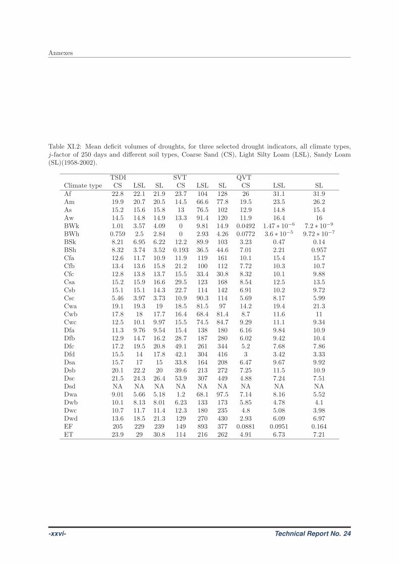
Annexes
Table XI.2: Mean deficit volumes of droughts, for three selected drought indicators, all climate types,j-factor of 250 days and different soil types, Coarse Sand (CS), Light Silty Loam (LSL), Sandy Loam(SL)(1958-2002).
TSDI SVT QVTClimate type CS LSL SL CS LSL SL CS LSL SLAf 22.8 22.1 21.9 23.7 104 128 26 31.1 31.9Am 19.9 20.7 20.5 14.5 66.6 77.8 19.5 23.5 26.2As 15.2 15.6 15.8 13 76.5 102 12.9 14.8 15.4Aw 14.5 14.8 14.9 13.3 91.4 120 11.9 16.4 16BWk 1.01 3.57 4.09 0 9.81 14.9 0.0492 1.47 ∗ 10−6 7.2 ∗ 10−9
BWh 0.759 2.5 2.84 0 2.93 4.26 0.0772 3.6 ∗ 10−5 9.72 ∗ 10−7
BSk 8.21 6.95 6.22 12.2 89.9 103 3.23 0.47 0.14BSh 8.32 3.74 3.52 0.193 36.5 44.6 7.01 2.21 0.957Cfa 12.6 11.7 10.9 11.9 119 161 10.1 15.4 15.7Cfb 13.4 13.6 15.8 21.2 100 112 7.72 10.3 10.7Cfc 12.8 13.8 13.7 15.5 33.4 30.8 8.32 10.1 9.88Csa 15.2 15.9 16.6 29.5 123 168 8.54 12.5 13.5Csb 15.1 15.1 14.3 22.7 114 142 6.91 10.2 9.72Csc 5.46 3.97 3.73 10.9 90.3 114 5.69 8.17 5.99Cwa 19.1 19.3 19 18.5 81.5 97 14.2 19.4 21.3Cwb 17.8 18 17.7 16.4 68.4 81.4 8.7 11.6 11Cwc 12.5 10.1 9.97 15.5 74.5 84.7 9.29 11.1 9.34Dfa 11.3 9.76 9.54 15.4 138 180 6.16 9.84 10.9Dfb 12.9 14.7 16.2 28.7 187 280 6.02 9.42 10.4Dfc 17.2 19.5 20.8 49.1 261 344 5.2 7.68 7.86Dfd 15.5 14 17.8 42.1 304 416 3 3.42 3.33Dsa 15.7 17 15 33.8 164 208 6.47 9.67 9.92Dsb 20.1 22.2 20 39.6 213 272 7.25 11.5 10.9Dsc 21.5 24.3 26.4 53.9 307 449 4.88 7.24 7.51Dsd NA NA NA NA NA NA NA NA NADwa 9.01 5.66 5.18 1.2 68.1 97.5 7.14 8.16 5.52Dwb 10.1 8.13 8.01 6.23 133 173 5.85 4.78 4.1Dwc 10.7 11.7 11.4 12.3 180 235 4.8 5.08 3.98Dwd 13.6 18.5 21.3 129 270 430 2.93 6.09 6.97EF 205 229 239 149 893 377 0.0881 0.0951 0.164ET 23.9 29 30.8 114 216 262 4.91 6.73 7.21
-xxvi- Technical Report No. 24
Annexes
XII Acronyms
ADI Aggregate Drought IndexASSM Accumulated Snow and Moisture ContentBFI Base Flow IndexCAFEC Climatically Appropriate For Existing ConditionsCDD Consecutive Dry DaysCMI Crop Moisture IndexCPA Cumulative Precipitation AnomalyEDI Effective Drought IndexFT Fixed ThresholdGHCN Global Historical Climatology NetworkGRACE Gravity Recovery And Climate ExperimentGRI Groundwater Resource IndexMAPVT Moving Average Precipitation with a Variable ThresholdNUT DAY Name of the synthetic modelPDSI Palmer Drought Severity IndexPHDI Palmer Hydrological Drought IndexQ DischargeQVT Discharge with a Variable ThresholdRAI Rainfall Anomaly IndexSMDI Soil Moisture Deficit IndexSPI Standardized Precipitation IndexSSI Standardized Streamflow IndexSVT Soil moisture Content with a Variable ThresholdSWSI Surface Water Supply IndexTSDI Total Storage Deficit IndexVIC Variable Infiltration CapacityVT Variable ThresholdWFD WATCH Forcing DataZ-index Palmer Moisture Anomaly Z-index
Technical Report No. 24 -xxvii-
Top Related
Copyright © 2022 FDOKUMEN

