


Bahasa
Halaman
Hukum

Viral abundanceandgenomesize distribution in the sedimentandwater columnofmarineand freshwaterecosystemsManuela Filippini1,2 & Mathias Middelboe1
1Marine Biological Laboratory, University of Copenhagen, Helsingør, Denmark; and 2Department of Aquatic Ecology, Eawag: Swiss Federal Institute of
Aquatic Science and Technology, and Institute of Integrative Biology (IBZ), ETH Zurich, Kastanienbaum, Switzerland
Correspondence: Mathias Middelboe,
Marine Biological Laboratory, University of
Copenhagen, Strandpromenaden 5, 3000
Helsing�r, Denmark. Tel.: 145 35 32 19 91;
fax: 145 35 32 19 51; e-mail:
Received 27 September 2006; revised 9 January
2007; accepted 15 January 2007.
First published online 28 March 2007.
DOI:10.1111/j.1574-6941.2007.00298.x
Editor: Patricia Sobecky
Keywords
pulsed field gel electrophoresis (PFGE); virus
community structure; sediment; freshwater;
marine; cross-system analysis.
Abstract
The size distribution of viral DNA in natural samples was investigated in a number
of marine, brackish and freshwater environments by means of pulsed field
gel electrophoresis (PFGE). The method was modified to work with both water
and sediment samples, with an estimated detection limit for individual virus
genome size groups of 1–2� 104 virus-like particles (VLP) mL�1 water and
2–4� 105 VLP cm�3 sediment in the original samples. Variations in the composi-
tion and distribution of dominant virus genome sizes were analyzed within
and between different habitats that covered a range in viral density from
0.4� 107 VLP mL�1 (sea water) to 300� 107 VLP cm�3 (lake sediment). The PFGE
community fingerprints showed a number of cross-system similarities in the
genome size distribution with a general dominance of genomes in the 30–48,
50–70 and 145–200 kb size fractions, and with many of the specific genome sizes
detected in all the investigated habitats. However, large differences in community
fingerprints were also observed between the investigated sites, and some virus
genome sizes were found only in specific biotopes (e.g. lake water), in specific
ecosystems (e.g. a particular lake) or even in specific microhabitats (e.g. a
particular sediment stratum).
Introduction
Viruses are ubiquitous and the most abundant biological
entities in aquatic ecosystems, with abundances typically in
the range of 107–108 virus-like particles (VLP) mL�1 in
pelagic environments and 108–109 VLP cm�3 in sediments
(e.g. Weinbauer, 2004; Suttle, 2005). Most of these viruses
are believed to be bacteriophages, accounting for a signifi-
cant part of prokaryotic mortality (e.g. Weinbauer, 2004;
Suttle, 2005). Increasing evidence suggests that viruses play
an important role in marine carbon cycling by mediating the
transformation of matter and energy in microbial food webs
through cell lysis (e.g. Wilhelm & Suttle, 1999; Riemann &
Middelboe, 2002a), and potentially influence microbial
diversity and community dynamics by the selective suppres-
sion of specific host populations (e.g. Thingstad & Lignell,
1997; Weinbauer & Rassoulzadegan, 2004).
Most studies of aquatic viruses have so far been carried
out in pelagic marine environments. However, viruses are
typically 10–100 fold more abundant in the sediment than in
the water column (Hewson et al., 2001; Danovaro & Serresi,
2002; Weinbauer, 2004), suggesting that they are important
players also in benthic systems, yet we still have relatively
limited and divergent observations on the role of viruses in
sediments: While most marine studies have found high
benthic viral activity and a significant impact of viruses on
benthic bacterial mortality (e.g. Hewson & Fuhrman, 2003;
Mei & Danovaro, 2004; Middelboe et al., 2006), a number of
studies from freshwater (e.g. Fischer et al., 2003; Filippini
et al., 2006) and other inland aquatic systems (Bettarel et al.,
2006) have found evidence of a low impact of viruses on in
the investigated sediments. These apparently contradicting
observations may be due to systematic differences in the role
of viruses for controlling bacterial mortality and biogeo-
chemical cycling in different benthic environments, empha-
sizing the need for further investigations on benthic viruses.
Until recently, viruses have been treated as a ‘black box’
with only little available information about the composition
and dynamics of environmental viral populations (e.g.
Wichels et al., 1998; Steward et al., 2000). Such information
about viral diversity and population dynamics on different
temporal and spatial scales is important, not only to resolve
the impact of viruses on bacterial community structure and
vice versa but also to understand the long term evolution
FEMS Microbiol Ecol 60 (2007) 397–410 c� 2007 Federation of European Microbiological SocietiesPublished by Blackwell Publishing Ltd. All rights reserved

and spreading of viruses in the environment. Viruses con-
stitute an enormous source of unexplored genetic informa-
tion (Suttle, 2005) and we are still in the early phase of
investigating the genetic composition, the spatial and tem-
poral distribution of individual virus populations and the
complex patterns of interactions between viruses and their
hosts.
Different approaches have been employed in the study of
virus diversity in aquatic systems. Examination of viral
diversity based on morphological characteristics obtained
by transmission electron microscopy has demonstrated a
large morphological variation (Corpe & Jensen, 1996), with
more than 80 different morphotypes observed in a single
lake (Finlay & Maberly, 2000). The use of PCR-based
methods to evaluate viral diversity has been restricted by
the absence of a conservative region shared among all
viruses. This approach has, however, been successfully
applied in the study of specific virus subgroups, such as
cyanophages, algal viruses and picorna-like viruses (e.g.
Culley et al., 2003). Most recently, metagenomic analyses of
viral DNA from environmental samples have provided the
first direct evidence of an enormous genetic diversity in
marine viral communities – an estimated 3000–7000 viral
types in 200 L of seawater (Breitbart et al., 2002) and
104–106 viral types in one kg of sediment (Breitbart et al.,
2004a) – with the most abundant types comprising only
2–3% and 0.01–0.1%, respectively, of the total viral com-
munity.
Pulsed field gel electrophoresis (PFGE) is another method
to analyze viral community composition (e.g. Steward &
Azam, 1999). This method provides a viral community
fingerprint based on the size distribution of dominant
genomes after separation of the genomes on an agarose gel
(Steward & Azam, 1999). Previous studies have demon-
strated that both viral community composition and the
relative intensity of individual bands can vary with season
(e.g. Wommack et al., 1999; Castberg et al., 2001; Larsen
et al., 2001, 2004; Sandaa & Larsen, 2006) and location (e.g.
Wommack et al., 1999; Riemann & Middelboe, 2002b),
illustrating that individual viral populations are dynamic
parts of pelagic microbial communities. On the other hand,
reports of only minor changes in the PFGE fingerprints
across large temporal and spatial scales despite several-fold
variations in general microbial abundance and activity
(Riemann & Middelboe, 2002b; Auguet et al., 2006) suggest
that part of the dominant viral genome sizes may be rather
persistent and perhaps permanently present in a given
ecosystem.
This approach has primarily been used in pelagic marine
waters (e.g. Wommack et al., 1999; Diez et al., 2000; Steward
et al., 2000; Fuhrman et al., 2002; Riemann & Middelboe,
2002b; Jiang et al., 2003, 2004; Sandaa et al., 2003) and to a
lesser extent in freshwaters (Auguet et al., 2006), whereas its
potential to describe benthic viral communities has not yet
been explored. One reason is likely to be that the critical
requirement for the clean preparation of viral DNA poses a
major challenge to the use of PFGE with sediment commu-
nities. Moreover, the majority of the pelagic PFGE studies
have been performed in marine environments, while a few
studies have investigated changes in PFGE patterns along
salinity gradients in estuarine systems (Riemann & Mid-
delboe, 2002b; Auguet et al., 2006). There exist, on the other
hand, to our knowledge no comparative analyses of PFGE
fingerprints between different environments, such as be-
tween water column and sediment communities, or between
lake communities and marine communities. It is therefore
not known to what extent specific ecosystems are character-
ized by a specific composition of dominant virus genome
sizes or whether there is an overlap in genome sizes between
environments.
The purpose of this study was therefore to (1) adapt and
apply the PFGE method to benthic viruses, and (2) investi-
gate patterns in viral genome size distribution obtained
from pelagic and benthic samples in a given ecosystem, and
from separate marine, brackish and freshwater environ-
ments.
Materials and methods
Study sites
Viral abundance, distribution and community structure was
studied in four different ecosystems between October 2004
and March 2005.
Lake Frederiksborg Slotss� is a small (0.21 km2) dimictic
and eutrophic lake with high sedimentation rate (Markager
et al., 1994) and an average depth of 3.1 m. The annual
primary production is c. 400 g C m�2 year�1 and the concen-
tration of dissolved organic carbon (DOC) ranges from 10
to 15 mg L�1 (Middelboe & S�ndergaard, 1993). Sediment
samples were collected at the deepest point (9 m) in the
centre of the lake.
Lake Esrum (17.3 km2) is the largest freshwater lake in
Denmark (maximum depth: 22 m, mean depth: 12.3 m). It
is meso-/eutrophic, with an annual primary production of
260 g C m�2 year�1 (S�ndergaard, 1991). Sediment samples
were collected in the center of the lake at 19.5 m water depth.
Niva Bay is a shallow (o 1 m), eutrophic coastal brackish
area, which is characterized by high input of organic matter
to the sediment, high benthic mineralization rates domi-
nated by sulfate-reducing bacteria (Middelboe et al., 2003),
and benthic primary production dominated by diatoms and
cyanobacteria.
Øresund is an estuarine sound characterized by a layer of
marine bottom water originating from the North Sea, which
is separated from the brackish surface layer by a pycnocline
FEMS Microbiol Ecol 60 (2007) 397–410c� 2007 Federation of European Microbiological SocietiesPublished by Blackwell Publishing Ltd. All rights reserved
398 M. Filippini & M. Middelboe
at 10–15 m depth. During winter, full mixing of the water
column occurs occasionally, and in this study water samples
were collected during such a mixing period. Mean annual
primary production in Øresund is about 240 g C m�2 year�1.
Two stations in Øresund were investigated: a shallow station
(10 m) which is exposed to the brackish surface water (only
collection of sediment samples) and a deeper site (26 m)
always situated below the pycnocline (collection of both
water and sediment samples).
Sampling
At each sampling site, 20 sediment cores containing the
upper 20 cm of sediment were collected (core diameter:
5.3 cm). Of these, 17 cores were used for the extraction of
viruses for community analysis at different sediment depths;
one core was used for determination of viral and bacterial
depth distribution, total carbon content and sediment
porosity, and two cores were used for measuring benthic
oxygen distribution and consumption. Along with the sedi-
ment samples, 20 L of surface water were collected from each
site. All samples were transported to the laboratory within
1–3 h after sampling and placed at in situ temperature.
Sediment characteristics
Sediment porosity (volume of water:volume of sediment)
was calculated from the specific sediment density and the
weight loss after drying at 105 1C for 24 h, and the total
organic carbon content was determined as the weight loss
after combustion at 450 1C for 24 h.
The type and size fractionation of the samples were
determined by sieving through different mesh sizes
according to Buchanan (1984). Twenty-five grams of oven-
dried sediment was placed in a beaker with 250 mL of tap
water, then 10 mL of aqueous sodium hexametaphosphate
(NaPO3)6 (6.2 g L�1) was added and the slurry stirred
mechanically for 15 min. The sediment was left overnight,
restirred the following morning for another 15 min and
sieved through a series of nested sieves (mesh sizes from
1 mm to 62mm). The different size fractions were dried at
100 1C and weighed.
Oxygen measurements
Oxygen microprofiles were measured in intact sediment
cores with a Clark type microelectrode with a depth resolu-
tion of 100mm. The signal of the electrode was detected by a
pico ampermeter. Total oxygen consumption in the cores
was measured according to Rasmussen & J�rgensen (1992)
as the linear decrease in oxygen concentration after capping
the submerged cores with a lid and insertion of a micro-
sensor into the core water.
Vertical profiles of total viral and bacterialabundance
The sediment cores were cut into 1–2 cm slices (a total of 6–13
samples) to determine the vertical distribution of viruses and
bacteria. The individual samples were manually homogenized
and a subsample (c. 4 g) was weighed and transferred to a
50 mL centrifuge tube, fixed with 4 mL of virus free water and
1 mL of glutaraldehyde (3% final concentration) and stored in
the dark at 5 1C for a maximum of 24 h. For extraction of
bacteria and viruses, sodium pyrophosphate (10 mM final
concentration) was added, and after 15 min the samples were
sonicated in a sonication bath for 2� 1 min before centrifuga-
tion for 5 min at 700 g (Glud & Middelboe, 2004). The
supernatant was collected and the sediment washed twice with
2 mL virus-free water. The total extracted volume was pooled
and a small volume of the virus-bacteria extract (50–100mL)
was filtered on to a 0.02-mm Anodisc filter (Whatman,
Maidstone, UK) and stained with SYBR Gold (Chen et al.,
2001). On each slide, 200–600 bacteria and viruses were
counted in 10–20 fields using epifluorescence microscopy at
� 1250 magnification. Previous evaluations of the accuracy of
this procedure from replicate samplings from the homoge-
nized sediment (Middelboe et al., 2003; Glud & Middelboe,
2004) have demonstrated that viral and bacterial abundance
are determined with an average accuracy of 5–6%. In this
study we have therefore applied this as a general accuracy of
the enumeration procedure.
Concentration of viruses from water samples
To obtain a sufficiently high density of viruses for PFGE
analyses, viruses from both water and sediment samples were
concentrated prior to analysis. For the water samples, 20 L of
water were filtered through first a GF/F filter (Whatman) and
then a 0.2-mm capsule filter (Type CCS-020-C1HS; Advantec,
Dublin, CA). Viruses were then concentrated to a final volume
of 100–200 mL by tangential flow filtration using a 30 K
Cartridge (PLTK Prep/ScaleTM-TFF 2.5 ft2 Cartridge, 30 K
regenerated cellulose membrane, Millipore, Bedford, MA).
Further concentration was carried out in 15 mL centrifugal
ultrafiltration devices (30 K Amicon Ultra, Millipore) to a final
volume of 4 mL. Viruses were then pelletted by ultracentrifu-
gation through a glycerol gradient (2 mL 5% glycerol on top of
2 mL 40% glycerol in a 5-mL tube) at 85.000 g for 98 min at
20 1C as described in Sambrook et al. (1989) (Beckman,
Fullerton, CA, Optima LE 80 k Ultracentrifuge; SW 55 Ti
Rotor). This purification step allowed only particles with a
sedimentation coefficient of 4 100 S to form a pellet, and has
shown to reduce the interference from unknown polymeric
material during electrophoresis (Riemann & Middelboe,
2002b). The supernatant was discarded, leaving c. 100mL above
the pellet. Hundred microliters of MSM (marine samples) or
SM buffer (freshwater samples) (Sambrook et al., 1989) and
FEMS Microbiol Ecol 60 (2007) 397–410 c� 2007 Federation of European Microbiological SocietiesPublished by Blackwell Publishing Ltd. All rights reserved
399Virus genome size distribution in aquatic systems
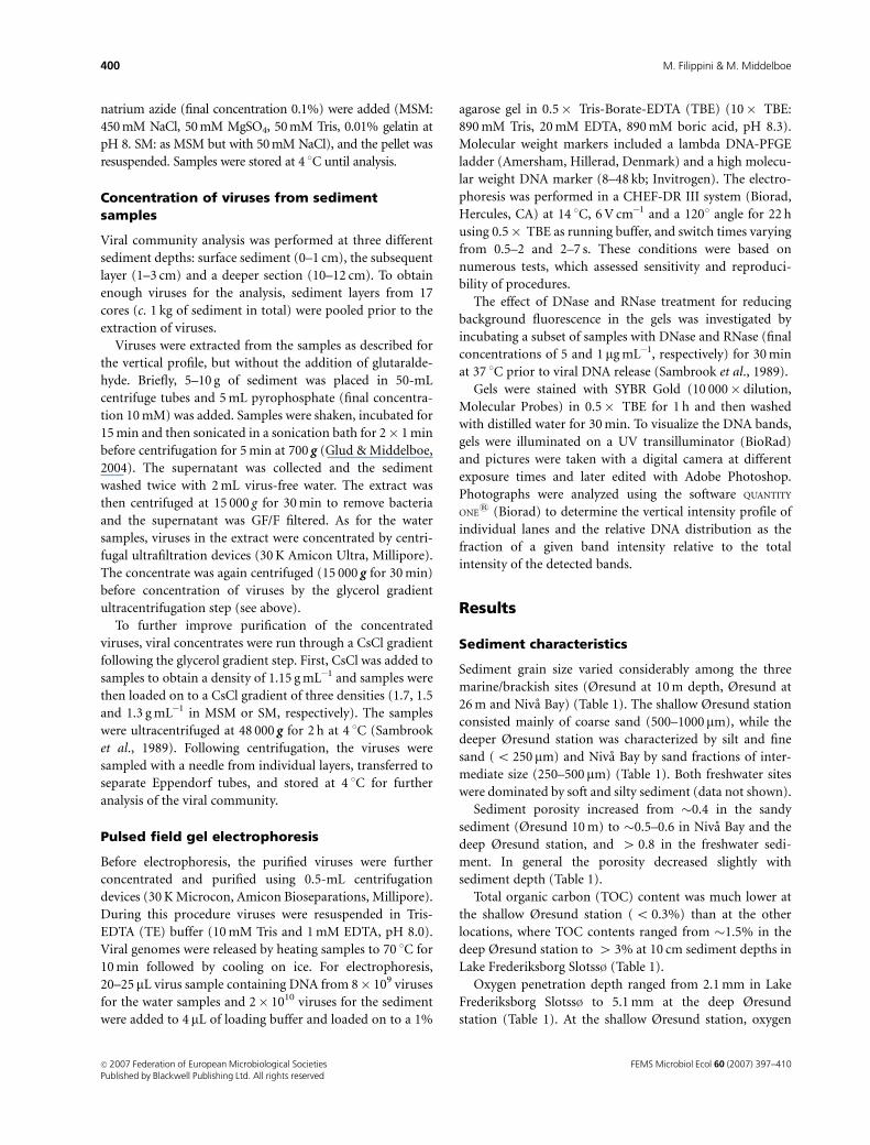
natrium azide (final concentration 0.1%) were added (MSM:
450 mM NaCl, 50 mM MgSO4, 50 mM Tris, 0.01% gelatin at
pH 8. SM: as MSM but with 50 mM NaCl), and the pellet was
resuspended. Samples were stored at 4 1C until analysis.
Concentration of viruses from sedimentsamples
Viral community analysis was performed at three different
sediment depths: surface sediment (0–1 cm), the subsequent
layer (1–3 cm) and a deeper section (10–12 cm). To obtain
enough viruses for the analysis, sediment layers from 17
cores (c. 1 kg of sediment in total) were pooled prior to the
extraction of viruses.
Viruses were extracted from the samples as described for
the vertical profile, but without the addition of glutaralde-
hyde. Briefly, 5–10 g of sediment was placed in 50-mL
centrifuge tubes and 5 mL pyrophosphate (final concentra-
tion 10 mM) was added. Samples were shaken, incubated for
15 min and then sonicated in a sonication bath for 2� 1 min
before centrifugation for 5 min at 700 g (Glud & Middelboe,
2004). The supernatant was collected and the sediment
washed twice with 2 mL virus-free water. The extract was
then centrifuged at 15 000 g for 30 min to remove bacteria
and the supernatant was GF/F filtered. As for the water
samples, viruses in the extract were concentrated by centri-
fugal ultrafiltration devices (30 K Amicon Ultra, Millipore).
The concentrate was again centrifuged (15 000 g for 30 min)
before concentration of viruses by the glycerol gradient
ultracentrifugation step (see above).
To further improve purification of the concentrated
viruses, viral concentrates were run through a CsCl gradient
following the glycerol gradient step. First, CsCl was added to
samples to obtain a density of 1.15 g mL�1 and samples were
then loaded on to a CsCl gradient of three densities (1.7, 1.5
and 1.3 g mL�1 in MSM or SM, respectively). The samples
were ultracentrifuged at 48 000 g for 2 h at 4 1C (Sambrook
et al., 1989). Following centrifugation, the viruses were
sampled with a needle from individual layers, transferred to
separate Eppendorf tubes, and stored at 4 1C for further
analysis of the viral community.
Pulsed field gel electrophoresis
Before electrophoresis, the purified viruses were further
concentrated and purified using 0.5-mL centrifugation
devices (30 K Microcon, Amicon Bioseparations, Millipore).
During this procedure viruses were resuspended in Tris-
EDTA (TE) buffer (10 mM Tris and 1 mM EDTA, pH 8.0).
Viral genomes were released by heating samples to 70 1C for
10 min followed by cooling on ice. For electrophoresis,
20–25 mL virus sample containing DNA from 8� 109 viruses
for the water samples and 2� 1010 viruses for the sediment
were added to 4 mL of loading buffer and loaded on to a 1%
agarose gel in 0.5� Tris-Borate-EDTA (TBE) (10� TBE:
890 mM Tris, 20 mM EDTA, 890 mM boric acid, pH 8.3).
Molecular weight markers included a lambda DNA-PFGE
ladder (Amersham, Hillerad, Denmark) and a high molecu-
lar weight DNA marker (8–48 kb; Invitrogen). The electro-
phoresis was performed in a CHEF-DR III system (Biorad,
Hercules, CA) at 14 1C, 6 V cm�1 and a 1201 angle for 22 h
using 0.5� TBE as running buffer, and switch times varying
from 0.5–2 and 2–7 s. These conditions were based on
numerous tests, which assessed sensitivity and reproduci-
bility of procedures.
The effect of DNase and RNase treatment for reducing
background fluorescence in the gels was investigated by
incubating a subset of samples with DNase and RNase (final
concentrations of 5 and 1 mg mL�1, respectively) for 30 min
at 37 1C prior to viral DNA release (Sambrook et al., 1989).
Gels were stained with SYBR Gold (10 000� dilution,
Molecular Probes) in 0.5� TBE for 1 h and then washed
with distilled water for 30 min. To visualize the DNA bands,
gels were illuminated on a UV transilluminator (BioRad)
and pictures were taken with a digital camera at different
exposure times and later edited with Adobe Photoshop.
Photographs were analyzed using the software QUANTITY
ONEs (Biorad) to determine the vertical intensity profile of
individual lanes and the relative DNA distribution as the
fraction of a given band intensity relative to the total
intensity of the detected bands.
Results
Sediment characteristics
Sediment grain size varied considerably among the three
marine/brackish sites (Øresund at 10 m depth, Øresund at
26 m and Niva Bay) (Table 1). The shallow Øresund station
consisted mainly of coarse sand (500–1000mm), while the
deeper Øresund station was characterized by silt and fine
sand (o 250 mm) and Niva Bay by sand fractions of inter-
mediate size (250–500 mm) (Table 1). Both freshwater sites
were dominated by soft and silty sediment (data not shown).
Sediment porosity increased from �0.4 in the sandy
sediment (Øresund 10 m) to �0.5–0.6 in Niva Bay and the
deep Øresund station, and 4 0.8 in the freshwater sedi-
ment. In general the porosity decreased slightly with
sediment depth (Table 1).
Total organic carbon (TOC) content was much lower at
the shallow Øresund station (o 0.3%) than at the other
locations, where TOC contents ranged from �1.5% in the
deep Øresund station to 4 3% at 10 cm sediment depths in
Lake Frederiksborg Slotss� (Table 1).
Oxygen penetration depth ranged from 2.1 mm in Lake
Frederiksborg Slotss� to 5.1 mm at the deep Øresund
station (Table 1). At the shallow Øresund station, oxygen
FEMS Microbiol Ecol 60 (2007) 397–410c� 2007 Federation of European Microbiological SocietiesPublished by Blackwell Publishing Ltd. All rights reserved
400 M. Filippini & M. Middelboe
penetration was much higher (4 3 cm), but because of
large sand particles it was impossible to measure accurately
with the microelectrodes used. The benthic mineralization
rate varied from a minimum of 14.7 mmol O2 m�2 day�1 in
the deep Øresund station to a maximum of 80.6 mmol
O2 m�2 day�1 in the eutrophic Lake Frederiksborg Slotss�,
with intermediate rates of 28–34 mmol O2 m�2 day�1 in
Lake Esrum, Niva Bay and the shallow Øresund station
(Table 1).
Distribution of viruses and bacteria
Large differences in total viral and bacterial abundances
were observed among locations. In general, viral and
bacteria abundances were higher in freshwater than in the
marine and brackish systems and at least 20-fold higher in
sediments than in the overlying water column (Fig. 1 and
Table 2). In the marine and brackish water samples, viral and
bacterial abundance ranged from 0.4 to 1.2� 107 VLP mL�1
and from 0.6 to 1.4� 106 mL�1, respectively. Viruses were
5–11 fold more abundant than bacteria (Table 2). In lake
water, viral abundance (3.8–15.7� 107 VLP mL�1) and the
virus:bacteria ratio (23–40) were higher than in the marine
and brackish water samples (Table 2).
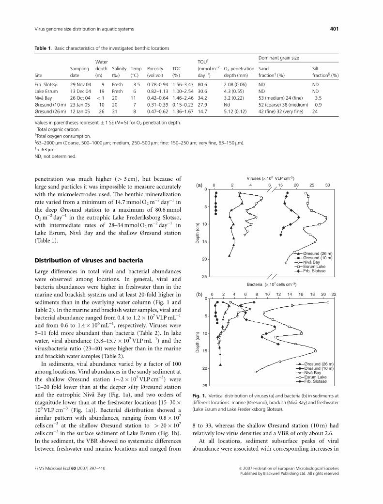
In sediments, viral abundance varied by a factor of 100
among locations. Viral abundances in the sandy sediment at
the shallow Øresund station (�2� 107 VLP cm�3) were
10–20 fold lower than at the deeper silty Øresund station
and the eutrophic Niva Bay (Fig. 1a), and two orders of
magnitude lower than at the freshwater locations [15–30�108 VLP cm�3 (Fig. 1a)]. Bacterial distribution showed a
similar pattern with abundances, ranging from 0.8� 107
cells cm�3 at the shallow Øresund station to 4 20� 107
cells cm�3 in the surface sediment of Lake Esrum (Fig. 1b).
In the sediment, the VBR showed no systematic differences
between freshwater and marine locations and ranged from
8 to 33, whereas the shallow Øresund station (10 m) had
relatively low virus densities and a VBR of only about 2.6.
At all locations, sediment subsurface peaks of viral
abundance were associated with corresponding increases in
Table 1. Basic characteristics of the investigated benthic locations
Site
Sampling
date
Water
depth
(m)
Salinity
(%)
Temp.
(1C)
Porosity
(vol:vol)
TOC�
(%)
TOUw
(mmol m�2
day�1)
O2 penetration
depth (mm)
Dominant grain size
Sand
fractionz (%)
Silt
fraction‰ (%)
Frb. Slotss� 29 Nov 04 9 Fresh 3.5 0.78–0.94 1.56–3.43 80.6 2.08 (0.06) ND ND
Lake Esrum 13 Dec 04 19 Fresh 6 0.82–1.13 1.00–2.54 30.6 4.3 (0.55) ND ND
Niva Bay 26 Oct 04 o 1 20 11 0.42–0.64 1.46–2.46 34.2 3.2 (0.22) 53 (medium) 24 (fine) 3.5
Øresund (10 m) 23 Jan 05 10 20 7 0.31–0.39 0.15–0.23 27.9 Nd 52 (coarse) 38 (medium) 0.9
Øresund (26 m) 12 Jan 05 26 31 8 0.47–0.62 1.36–1.67 14.7 5.12 (0.12) 42 (fine) 32 (very fine) 24
Values in parentheses represent � 1 SE (N = 5) for O2 penetration depth.�Total organic carbon.wTotal oxygen consumption.z63–2000 mm (Coarse, 500–1000mm; medium, 250–500mm; fine: 150–250 mm; very fine, 63–150 mm).‰o 63 mm.
ND, not determined.
Viruses (× 10 VLP cm )
0 2 4 6 15 20 25 30
Dep
th (
cm)
0(a)
(b)
5
10
15
20
25
Øresund (26 m)Øresund (10 m)Nivå BayEsrum Lake Frb. Slotssø
Øresund (26 m)Øresund (10 m)Nivå BayEsrum Lake Frb. Slotssø
Bacteria (× 10 cells cm )
0 2 4 6 8 10 12 14 16 18 20 22
Dep
th (
cm)
0
5
10
15
20
25
Fig. 1. Vertical distribution of viruses (a) and bacteria (b) in sediments at
different locations: marine (Øresund), brackish (Niva Bay) and freshwater
(Lake Esrum and Lake Frederiksborg Slotssø).
FEMS Microbiol Ecol 60 (2007) 397–410 c� 2007 Federation of European Microbiological SocietiesPublished by Blackwell Publishing Ltd. All rights reserved
401Virus genome size distribution in aquatic systems
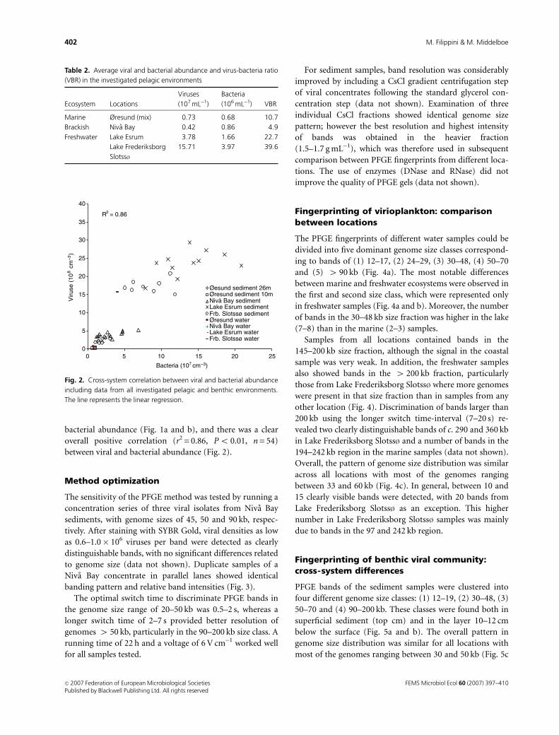
bacterial abundance (Fig. 1a and b), and there was a clear
overall positive correlation (r2 = 0.86, Po 0.01, n = 54)
between viral and bacterial abundance (Fig. 2).
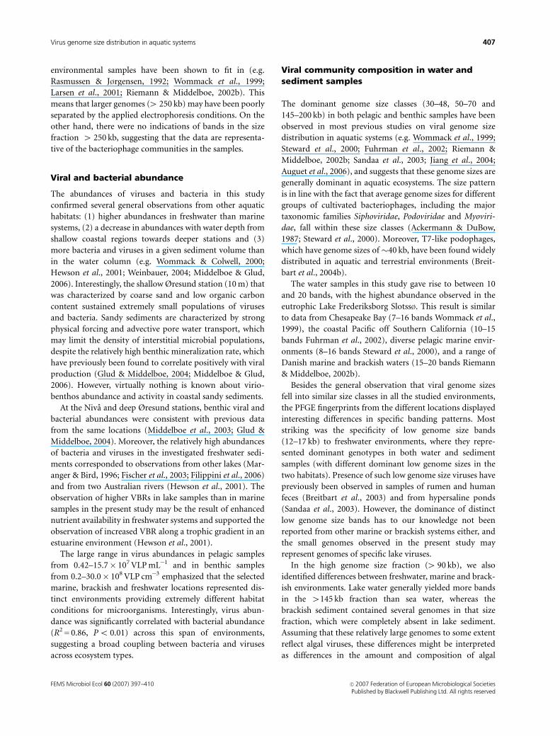
Method optimization
The sensitivity of the PFGE method was tested by running a
concentration series of three viral isolates from Niva Bay
sediments, with genome sizes of 45, 50 and 90 kb, respec-
tively. After staining with SYBR Gold, viral densities as low
as 0.6–1.0� 106 viruses per band were detected as clearly
distinguishable bands, with no significant differences related
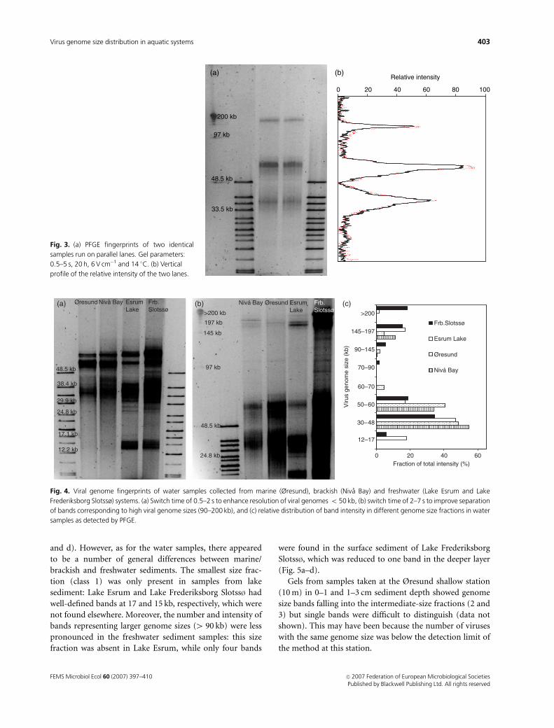
to genome size (data not shown). Duplicate samples of a
Niva Bay concentrate in parallel lanes showed identical
banding pattern and relative band intensities (Fig. 3).
The optimal switch time to discriminate PFGE bands in
the genome size range of 20–50 kb was 0.5–2 s, whereas a
longer switch time of 2–7 s provided better resolution of
genomes 4 50 kb, particularly in the 90–200 kb size class. A
running time of 22 h and a voltage of 6 V cm�1 worked well
for all samples tested.
For sediment samples, band resolution was considerably
improved by including a CsCl gradient centrifugation step
of viral concentrates following the standard glycerol con-
centration step (data not shown). Examination of three
individual CsCl fractions showed identical genome size
pattern; however the best resolution and highest intensity
of bands was obtained in the heavier fraction
(1.5–1.7 g mL�1), which was therefore used in subsequent
comparison between PFGE fingerprints from different loca-
tions. The use of enzymes (DNase and RNase) did not
improve the quality of PFGE gels (data not shown).
Fingerprinting of virioplankton: comparisonbetween locations
The PFGE fingerprints of different water samples could be
divided into five dominant genome size classes correspond-
ing to bands of (1) 12–17, (2) 24–29, (3) 30–48, (4) 50–70
and (5) 4 90 kb (Fig. 4a). The most notable differences
between marine and freshwater ecosystems were observed in
the first and second size class, which were represented only
in freshwater samples (Fig. 4a and b). Moreover, the number
of bands in the 30–48 kb size fraction was higher in the lake
(7–8) than in the marine (2–3) samples.
Samples from all locations contained bands in the
145–200 kb size fraction, although the signal in the coastal
sample was very weak. In addition, the freshwater samples
also showed bands in the 4 200 kb fraction, particularly
those from Lake Frederiksborg Slotss� where more genomes
were present in that size fraction than in samples from any
other location (Fig. 4). Discrimination of bands larger than
200 kb using the longer switch time-interval (7–20 s) re-
vealed two clearly distinguishable bands of c. 290 and 360 kb
in Lake Frederiksborg Slotss� and a number of bands in the
194–242 kb region in the marine samples (data not shown).
Overall, the pattern of genome size distribution was similar
across all locations with most of the genomes ranging
between 33 and 60 kb (Fig. 4c). In general, between 10 and
15 clearly visible bands were detected, with 20 bands from
Lake Frederiksborg Slotss� as an exception. This higher
number in Lake Frederiksborg Slotss� samples was mainly
due to bands in the 97 and 242 kb region.
Fingerprinting of benthic viral community:cross-system differences
PFGE bands of the sediment samples were clustered into
four different genome size classes: (1) 12–19, (2) 30–48, (3)
50–70 and (4) 90–200 kb. These classes were found both in
superficial sediment (top cm) and in the layer 10–12 cm
below the surface (Fig. 5a and b). The overall pattern in
genome size distribution was similar for all locations with
most of the genomes ranging between 30 and 50 kb (Fig. 5c
Table 2. Average viral and bacterial abundance and virus-bacteria ratio
(VBR) in the investigated pelagic environments
Ecosystem Locations
Viruses
(107 mL�1)
Bacteria
(106 mL�1) VBR
Marine Øresund (mix) 0.73 0.68 10.7
Brackish Niva Bay 0.42 0.86 4.9
Freshwater Lake Esrum 3.78 1.66 22.7
Lake Frederiksborg
Slotss�
15.71 3.97 39.6
0
5
10
15
20
25
30
35
40
0 5 10 15 20 25
Bacteria (10 cm )
Viru
se (
10
cm
)
Øesund sediment 26mØresund sediment 10mNivå Bay sedimentLake Esrum sedimentFrb. Slotssø sedimentØresund waterNivå Bay waterLake Esrum waterFrb. Slotssø water
R = 0.86
Fig. 2. Cross-system correlation between viral and bacterial abundance
including data from all investigated pelagic and benthic environments.
The line represents the linear regression.
FEMS Microbiol Ecol 60 (2007) 397–410c� 2007 Federation of European Microbiological SocietiesPublished by Blackwell Publishing Ltd. All rights reserved
402 M. Filippini & M. Middelboe
and d). However, as for the water samples, there appeared
to be a number of general differences between marine/
brackish and freshwater sediments. The smallest size frac-
tion (class 1) was only present in samples from lake
sediment: Lake Esrum and Lake Frederiksborg Slotss� had
well-defined bands at 17 and 15 kb, respectively, which were
not found elsewhere. Moreover, the number and intensity of
bands representing larger genome sizes (4 90 kb) were less
pronounced in the freshwater sediment samples: this size
fraction was absent in Lake Esrum, while only four bands
were found in the surface sediment of Lake Frederiksborg
Slotss�, which was reduced to one band in the deeper layer
(Fig. 5a–d).
Gels from samples taken at the Øresund shallow station
(10 m) in 0–1 and 1–3 cm sediment depth showed genome
size bands falling into the intermediate-size fractions (2 and
3) but single bands were difficult to distinguish (data not
shown). This may have been because the number of viruses
with the same genome size was below the detection limit of
the method at this station.
0 20 40 60
12–17
30–48
50–60
60–70
70–90
90–145
145–197
>200
Viru
s ge
nom
e si
ze (
kb)
Fraction of total intensity (%)
Frb.Slotssø
Esrum Lake
Øresund
Nivå Bay
Nivå BayNivå Bay EsrumLake
EsrumLake
Frb.Slotssø
Frb.Slotssø
ØresundØresund
48.5 kb
38.4 kb
17.1 kb
12.2 kb24.8 kb
48.5 kb
97 kb
145 kb
197 kb
>200 kb
29.9 kb
24.8 kb
(a) (b) (c)
Fig. 4. Viral genome fingerprints of water samples collected from marine (Øresund), brackish (Niva Bay) and freshwater (Lake Esrum and Lake
Frederiksborg Slotssø) systems. (a) Switch time of 0.5–2 s to enhance resolution of viral genomes o 50 kb, (b) switch time of 2–7 s to improve separation
of bands corresponding to high viral genome sizes (90–200 kb), and (c) relative distribution of band intensity in different genome size fractions in water
samples as detected by PFGE.
Relative intensity
0 20 40 60 80 100
200 kb
97 kb
48.5 kb
33.5 kb
(a) (b)
Fig. 3. (a) PFGE fingerprints of two identical
samples run on parallel lanes. Gel parameters:
0.5–5 s, 20 h, 6 V cm�1 and 14 1C. (b) Vertical
profile of the relative intensity of the two lanes.
FEMS Microbiol Ecol 60 (2007) 397–410 c� 2007 Federation of European Microbiological SocietiesPublished by Blackwell Publishing Ltd. All rights reserved
403Virus genome size distribution in aquatic systems
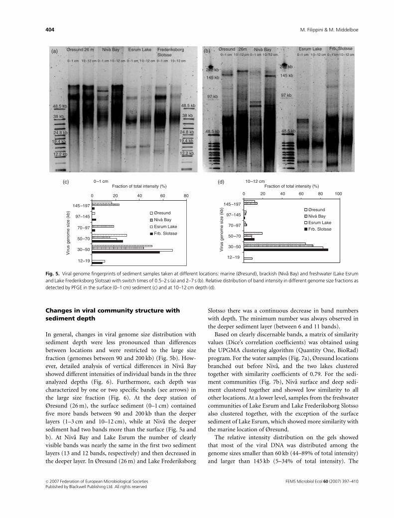
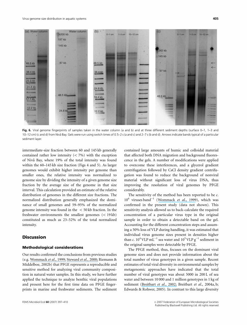
Changes in viral community structure withsediment depth
In general, changes in viral genome size distribution with
sediment depth were less pronounced than differences
between locations and were restricted to the large size
fraction (genomes between 90 and 200 kb) (Fig. 5b). How-
ever, detailed analysis of vertical differences in Niva Bay
showed different intensities of individual bands in the three
analyzed depths (Fig. 6). Furthermore, each depth was
characterized by one or two specific bands (see arrows) in
the large size fraction (Fig. 6). At the deep station of
Øresund (26 m), the surface sediment (0–1 cm) contained
five more bands between 90 and 200 kb than the deeper
layers (1–3 cm and 10–12 cm), while at Niva the deeper
sediment had two bands more than the surface (Fig. 5a and
b). At Niva Bay and Lake Esrum the number of clearly
visible bands was nearly the same in the first two sediment
layers (13 and 12 bands, respectively) and then decreased in
the deeper layer. In Øresund (26 m) and Lake Frederiksborg
Slotss� there was a continuous decrease in band numbers
with depth. The minimum number was always observed in
the deeper sediment layer (between 6 and 11 bands).
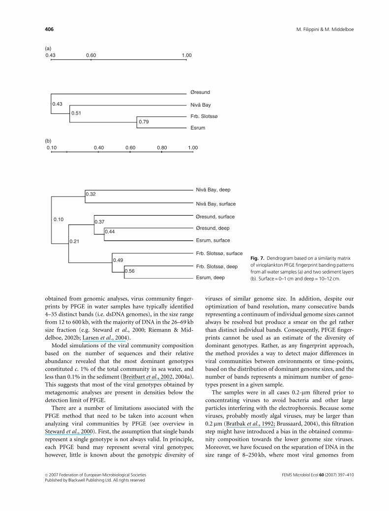
Based on clearly discernable bands, a matrix of similarity
values (Dice’s correlation coefficients) was obtained using
the UPGMA clustering algorithm (Quantity One, BioRad)
program. For the water samples (Fig. 7a), Øresund locations
branched out before Niva, and the two lakes clustered
together with similarity coefficients of 0.79. For the sedi-
ment communities (Fig. 7b), Niva surface and deep sedi-
ment clustered together and showed low similarity to all
other locations. At a lower level, samples from the freshwater
communities of Lake Esrum and Lake Frederiksborg Slotss�
also clustered together, with the exception of the surface
sediment of Lake Esrum, which showed more similarity with
the marine location of Øresund.
The relative intensity distribution on the gels showed
that most of the viral DNA was distributed among the
genome sizes smaller than 60 kb (44–89% of total intensity)
and larger than 145 kb (5–34% of total intensity). The
0–1 cm
0 20 40 60 80
145–197
97–145
70–97
50–70
30–50
12–19
Viru
s ge
nom
e si
ze (
kb)
Fraction of total intensity (%)
Øresund
Nivå Bay
Esrum Lake
Frb. Slotssø
10–12 cm
0 20 40 60 80 100
145–197
97–145
70–97
50–70
30–50
12–19
Viru
s ge
nom
e si
ze (
kb)
Fraction of total intensity (%)
Øresund
Nivå Bay
Esrum Lake
Frb. Slotssø
Nivå Bay Esrum Lake FrederiksborgSlotssø
Øresund 26 m Nivå Bay Esrum Lake Frb. SlotssøØresund 26m
48.5 kb
38 kb
19.4 kb
12.2 kb12.2 kb
19.4 kb
24.8 kb
97 kb
145 kb
242 kb242 kb
145 kb
97 kb
48.5 kb
48.5 kb48.5 kb
38 kb
24.8 kb
(a)
(c) (d)
(b)
Fig. 5. Viral genome fingerprints of sediment samples taken at different locations: marine (Øresund), brackish (Niva Bay) and freshwater (Lake Esrum
and Lake Frederiksborg Slotssø) with switch times of 0.5–2 s (a) and 2–7 s (b). Relative distribution of band intensity in different genome size fractions as
detected by PFGE in the surface (0–1 cm) sediment (c) and at 10–12 cm depth (d).
FEMS Microbiol Ecol 60 (2007) 397–410c� 2007 Federation of European Microbiological SocietiesPublished by Blackwell Publishing Ltd. All rights reserved
404 M. Filippini & M. Middelboe
intermediate-size fraction between 60 and 145 kb generally
contained rather low intensity (o 7%) with the exception
of Niva Bay, where 19% of the total intensity was found
within the 60–145 kb size fraction (Figs 4 and 5). As larger
genomes would exhibit higher intensity per genome than
smaller ones, the relative intensity was normalized to
genome size by dividing the intensity of a given genome size
fraction by the average size of the genome in that size
interval. This calculation provided an estimate of the relative
distribution of genomes in the different size fractions. The
normalized distribution generally emphasized the domi-
nance of small genomes and 59–95% of the normalized
genome intensity was found in the o 50 kb fraction. In the
freshwater environments the smallest genomes (o 19 kb)
constituted as much as 23–52% of the total normalized
intensity.
Discussion
Methodological considerations
Our results confirmed the conclusions from previous studies
(e.g. Wommack et al., 1999; Steward et al., 2000; Riemann &
Middelboe, 2002b) that PFGE represents a reproducible and
sensitive method for analyzing viral community composi-
tion in natural water samples. In this study, we have further
applied the technique to analyze benthic viral populations
and present here for the first time data on PFGE finger-
prints in marine and freshwater sediments. The sediment
contained large amounts of humic and colloidal material
that affected both DNA migration and background fluores-
cence in the gels. A number of modifications were applied
to overcome these interferences, and a glycerol gradient
centrifugation followed by CsCl density gradient centrifu-
gation was found to reduce the background of nonviral
material without significant loss of virus DNA, thus
improving the resolution of viral genomes by PFGE
considerably.
The sensitivity of the method has been reported to be c.
106 viruses band�1 (Wommack et al., 1999), which was
confirmed in the present study (data not shown). This
sensitivity analysis allowed us to back-calculate the required
concentration of a particular virus type in the original
sample in order to obtain a detectable band on the gel.
Accounting for the different concentration steps and assum-
ing a 50% loss of VLP during handling, it was estimated that
individual virus genome sizes present in densities higher
than c. 104 VLP mL�1 sea water and 105 VLP g�1 sediment in
the original samples were detectable by PFGE.
The PFGE method, thus, focuses on the dominant viral
genome sizes and does not provide information about the
total number of virus genotypes in a given sample. Recent
estimates of total viral diversity in environmental samples by
metagenomic approaches have indicated that the total
number of viral genotypes was about 5000 in 200 L of sea
water and between 10 000 and 1 million genotypes in 1 kg of
sediment (Breitbart et al., 2002; Breitbart et al., 2004a, b;
Edwards & Rohwer, 2005). In contrast to this large diversity
Water column Water column
48.5 kb
48.5 kb19.4 kb
12.2 kb12.2 kb
17.1 kb
29.9 kb
24.8 kb
242 kb
145 kb
97 kb
48.5 kb
38.4 kb38.4 kb
48.5 kb
24.8 kb
24.8 kb
97 kb
197 kb
(a) (b) (c)
145 kb
>200 kb
Fig. 6. Viral genome fingerprints of samples taken in the water column (a and b) and at three different sediment depths (surface 0–1, 1–3 and
10–12 cm) (c and d) from Niva Bay. Gels were run using switch times of 0.5–2 s (a and c) and 2–7 s (b and d). Arrows indicate bands typical of a particular
sediment layer.
FEMS Microbiol Ecol 60 (2007) 397–410 c� 2007 Federation of European Microbiological SocietiesPublished by Blackwell Publishing Ltd. All rights reserved
405Virus genome size distribution in aquatic systems
obtained from genomic analyses, virus community finger-
prints by PFGE in water samples have typically identified
4–35 distinct bands (i.e. dsDNA genomes), in the size range
from 12 to 600 kb, with the majority of DNA in the 26–69 kb
size fraction (e.g. Steward et al., 2000; Riemann & Mid-
delboe, 2002b; Larsen et al., 2004).
Model simulations of the viral community composition
based on the number of sequences and their relative
abundance revealed that the most dominant genotypes
constituted c. 1% of the total community in sea water, and
less than 0.1% in the sediment (Breitbart et al., 2002, 2004a).
This suggests that most of the viral genotypes obtained by
metagenomic analyses are present in densities below the
detection limit of PFGE.
There are a number of limitations associated with the
PFGE method that need to be taken into account when
analyzing viral communities by PFGE (see overview in
Steward et al., 2000). First, the assumption that single bands
represent a single genotype is not always valid. In principle,
each PFGE band may represent several viral genotypes;
however, little is known about the genotypic diversity of
viruses of similar genome size. In addition, despite our
optimization of band resolution, many consecutive bands
representing a continuum of individual genome sizes cannot
always be resolved but produce a smear on the gel rather
than distinct individual bands. Consequently, PFGE finger-
prints cannot be used as an estimate of the diversity of
dominant genotypes. Rather, as any fingerprint approach,
the method provides a way to detect major differences in
viral communities between environments or time-points,
based on the distribution of dominant genome sizes, and the
number of bands represents a minimum number of geno-
types present in a given sample.
The samples were in all cases 0.2-mm filtered prior to
concentrating viruses to avoid bacteria and other large
particles interfering with the electrophoresis. Because some
viruses, probably mostly algal viruses, may be larger than
0.2 mm (Bratbak et al., 1992; Brussaard, 2004), this filtration
step might have introduced a bias in the obtained commu-
nity composition towards the lower genome size viruses.
Moreover, we have focused on the separation of DNA in the
size range of 8–250 kb, where most viral genomes from
(a)
(b)
Øresund
Nivå Bay
Esrum
Frb. Slotssø
Nivå Bay, deep
Nivå Bay, surface
Øresund, surface
Øresund, deep
Esrum, deep
Frb. Slotssø, surface
Esrum, surface
Frb. Slotssø, deep
0.10
0.21
0.32
0.43
0.43
0.51
0.79
0.10 0.40 0.60
0.60
0.80 1.00
1.00
0.37
0.44
0.49
0.56
Fig. 7. Dendrogram based on a similarity matrix
of virioplankton PFGE fingerprint banding patterns
from all water samples (a) and two sediment layers
(b). Surface = 0–1 cm and deep = 10–12 cm.
FEMS Microbiol Ecol 60 (2007) 397–410c� 2007 Federation of European Microbiological SocietiesPublished by Blackwell Publishing Ltd. All rights reserved
406 M. Filippini & M. Middelboe
environmental samples have been shown to fit in (e.g.
Rasmussen & J�rgensen, 1992; Wommack et al., 1999;
Larsen et al., 2001; Riemann & Middelboe, 2002b). This
means that larger genomes (4 250 kb) may have been poorly
separated by the applied electrophoresis conditions. On the
other hand, there were no indications of bands in the size
fraction 4 250 kb, suggesting that the data are representa-
tive of the bacteriophage communities in the samples.
Viral and bacterial abundance
The abundances of viruses and bacteria in this study
confirmed several general observations from other aquatic
habitats: (1) higher abundances in freshwater than marine
systems, (2) a decrease in abundances with water depth from
shallow coastal regions towards deeper stations and (3)
more bacteria and viruses in a given sediment volume than
in the water column (e.g. Wommack & Colwell, 2000;
Hewson et al., 2001; Weinbauer, 2004; Middelboe & Glud,
2006). Interestingly, the shallow Øresund station (10 m) that
was characterized by coarse sand and low organic carbon
content sustained extremely small populations of viruses
and bacteria. Sandy sediments are characterized by strong
physical forcing and advective pore water transport, which
may limit the density of interstitial microbial populations,
despite the relatively high benthic mineralization rate, which
have previously been found to correlate positively with viral
production (Glud & Middelboe, 2004; Middelboe & Glud,
2006). However, virtually nothing is known about virio-
benthos abundance and activity in coastal sandy sediments.
At the Niva and deep Øresund stations, benthic viral and
bacterial abundances were consistent with previous data
from the same locations (Middelboe et al., 2003; Glud &
Middelboe, 2004). Moreover, the relatively high abundances
of bacteria and viruses in the investigated freshwater sedi-
ments corresponded to observations from other lakes (Mar-
anger & Bird, 1996; Fischer et al., 2003; Filippini et al., 2006)
and from two Australian rivers (Hewson et al., 2001). The
observation of higher VBRs in lake samples than in marine
samples in the present study may be the result of enhanced
nutrient availability in freshwater systems and supported the
observation of increased VBR along a trophic gradient in an
estuarine environment (Hewson et al., 2001).
The large range in virus abundances in pelagic samples
from 0.42–15.7� 107 VLP mL�1 and in benthic samples
from 0.2–30.0� 108 VLP cm�3 emphasized that the selected
marine, brackish and freshwater locations represented dis-
tinct environments providing extremely different habitat
conditions for microorganisms. Interestingly, virus abun-
dance was significantly correlated with bacterial abundance
(R2 = 0.86, Po 0.01) across this span of environments,
suggesting a broad coupling between bacteria and viruses
across ecosystem types.
Viral community composition in water andsediment samples
The dominant genome size classes (30–48, 50–70 and
145–200 kb) in both pelagic and benthic samples have been
observed in most previous studies on viral genome size
distribution in aquatic systems (e.g. Wommack et al., 1999;
Steward et al., 2000; Fuhrman et al., 2002; Riemann &
Middelboe, 2002b; Sandaa et al., 2003; Jiang et al., 2004;
Auguet et al., 2006), and suggests that these genome sizes are
generally dominant in aquatic ecosystems. The size pattern
is in line with the fact that average genome sizes for different
groups of cultivated bacteriophages, including the major
taxonomic families Siphoviridae, Podoviridae and Myoviri-
dae, fall within these size classes (Ackermann & DuBow,
1987; Steward et al., 2000). Moreover, T7-like podophages,
which have genome sizes of �40 kb, have been found widely
distributed in aquatic and terrestrial environments (Breit-
bart et al., 2004b).
The water samples in this study gave rise to between 10
and 20 bands, with the highest abundance observed in the
eutrophic Lake Frederiksborg Slotss�. This result is similar
to data from Chesapeake Bay (7–16 bands Wommack et al.,
1999), the coastal Pacific off Southern California (10–15
bands Fuhrman et al., 2002), diverse pelagic marine envir-
onments (8–16 bands Steward et al., 2000), and a range of
Danish marine and brackish waters (15–20 bands Riemann
& Middelboe, 2002b).
Besides the general observation that viral genome sizes
fell into similar size classes in all the studied environments,
the PFGE fingerprints from the different locations displayed
interesting differences in specific banding patterns. Most
striking was the specificity of low genome size bands
(12–17 kb) to freshwater environments, where they repre-
sented dominant genotypes in both water and sediment
samples (with different dominant low genome sizes in the
two habitats). Presence of such low genome size viruses have
previously been observed in samples of rumen and human
feces (Breitbart et al., 2003) and from hypersaline ponds
(Sandaa et al., 2003). However, the dominance of distinct
low genome size bands has to our knowledge not been
reported from other marine or brackish systems either, and
the small genomes observed in the present study may
represent genomes of specific lake viruses.
In the high genome size fraction (4 90 kb), we also
identified differences between freshwater, marine and brack-
ish environments. Lake water generally yielded more bands
in the 4145 kb fraction than sea water, whereas the
brackish sediment contained several genomes in that size
fraction, which were completely absent in lake sediment.
Assuming that these relatively large genomes to some extent
reflect algal viruses, these differences might be interpreted
as differences in the amount and composition of algal
FEMS Microbiol Ecol 60 (2007) 397–410 c� 2007 Federation of European Microbiological SocietiesPublished by Blackwell Publishing Ltd. All rights reserved
407Virus genome size distribution in aquatic systems

populations in the systems. Both lakes have generally high
pelagic algal biomass compared with the marine locations,
whereas benthic algae were absent because of low light
penetration and anoxic conditions prevailing in the bottom
water layer. The Niva Bay sediment, on the other hand,
harbors active diatom and cyanobacterial communities, and
also the coastal aphotic sediment is known to contain large
abundances of living phytoplankton cells that may survive
for several months in the sediment (Hansen & Josefson,
2001). Consequently, the similarity analysis showed that the
freshwater (Lake Frederiksborg Slotss� and Lake Esrum), the
brackish (Niva Bay) and the marine (Øresund) environ-
ments branched out separately in the similarity index, with
relatively low similarity between environments and even
within individual sampling sites.
A comparison of the PFGE profiles from pelagic and
benthic samples demonstrated that a number of bands,
especially in the 48–60 kb size fraction, were observed on
both environments. This may suggest that some of the
benthic viruses may originate from pelagic viruses that fall
out of the water column on sedimenting particles. Previous
estimates of the input of pelagic viruses to the sediment
indicated that this process could only account for a very
small fraction of the daily viral production in the investi-
gated sediment (Hewson & Fuhrman, 2003). Obviously, this
depends both on the rate of sedimentation and the ability of
viruses produced in the water column to maintain popula-
tions within the sediment, and still virtually nothing is
known about the fate of pelagic viruses when they reach the
sediment.
Although there was a large overlap in PFGE fingerprints
from pelagic and benthic samples from the same environ-
ment as well as from different environments, each habitat
also contained genomes that seemed to be specific for that
particular environment. In the intermediate genome size
fraction (70–100 kb), large differences were observed be-
tween sediment and water samples with a number of distinct
bands occurring in the sediment, which were absent from
the water samples. Even within a given sediment, small
differences in 70–100 kb banding patterns were observed
with depth, where specific bands were present in specific
depths. This suggests that the some benthic viral popula-
tions are associated with specific stratifications in the
microbial communities.
Consequently, even though some genome sizes were
present in all the samples, the viral communities, as de-
scribed by PFGE, varied considerably between different
samples. It should be noted, however, that our samples
taken at a single occasion are not fully representative of the
investigated sites. Some of the observed differences between
samples therefore might reflect temporal or spatial variation
within a given location rather than actual differences
between systems.
The total number of bands also decreased with sediment
depth, probably reflecting that specific viral genome sizes
decreased to below detection limit in the deeper sediments,
which might be a benthic parallel to the decrease in band
numbers with water depths from 5 to 500 m in the pelagic
ocean (Fuhrman et al., 2002).
In conclusion, PFGE can be useful to obtain viral genome
size fingerprints not only of pelagic water samples but also of
sediment samples, and we present here for the first time a
direct comparison of PFGE fingerprints from pelagic and
benthic habitats within and between ecosystems. Data from
marine, brackish and freshwater systems showed similarities
in genome size distribution between a number of habitats
covering a large range of microbial activities and abun-
dances. However, PFGE analysis also indicated that certain
genome sizes were found only in certain types of environ-
ments (e.g. lake water), in certain locations (e.g. a particular
lake) or even in certain microhabitats (e.g. a particular
sediment layer). The results suggest that some virus pheno-
types are ubiquitous in aquatic systems and may be effi-
ciently spread between environments, while the distribution
of others may be limited to certain environments or condi-
tions. However, more advanced genetic tools are necessary
for providing further insight to the genotypic composition
and spatial dynamics of natural viral communities.
Acknowledgements
We thank Benly True and Brian Green for help with
collecting the marine samples and Anni Glud for prepara-
tion and help with oxygen microsensors. Mark O. Gessner
provided valuable comments on the manuscript. The study
was supported by the Danish Natural Sciences Research
Council.
References
Ackermann HW & DuBow MS (1987) Viruses of Prokaryotes:
Natural Groups of Bacteriophages. CRC Press, Inc., Boca Raton,
FL.
Auguet JC, Montanie H & Lebaron P (2006) Structure of
virioplankton in the Charente estuary (France): transmission
electron microscopy versus pulsed field gel electrophoresis.
Microb Ecol 51: 197–208.
Bettarel Y, Bouvy M, Dumont C & Sime-Ngando T (2006) Virus-
bacterium interactions in water and sediment of West African
inland aquatic systems. Appl Environ Microbiol 72: 5274–5258.
Bratbak G, Haslund OH, Heldal M, Næs A & R�eggen T (1992)
Giant marine viruses? Mar Ecol Prog Ser 85: 201–202.
Breitbart M, Salamon P, Andersen B, Mahaffy JM, Sagall AM,
Mead D, Azam F & Rohwer F (2002) Genomic analysis of
uncultured marine viral communities. PNAS 99:
14250–14255.
FEMS Microbiol Ecol 60 (2007) 397–410c� 2007 Federation of European Microbiological SocietiesPublished by Blackwell Publishing Ltd. All rights reserved
408 M. Filippini & M. Middelboe
Breitbart M, Hewson I, Felts B, Mahaffy JM, Nulton J, Salamon P
& Rohwer F (2003) Metagenomic analysis of an uncultured
viral community from human feces. J Bacteriol 185:
6220–6223.
Breitbart M, Felts B, Kelley S, Mahaffy J, Nulton J, Salamon P &
Rohwer F (2004a) Diversity and population structure of a
near-shore marine sediment viral community. Proc R Soc Lond
B 271: 565–574.
Breitbart M, Miyake JH & Rohwer F (2004b) Global distribution
of nearly identical phage-encoded DNA sequences. FEMS
Microbiol Lett 236: 249–256.
Brussaard CPD (2004) Viral control of phytoplankton
populations – a review. J Eukariot Microbiol 51: 125–138.
Buchanan JB (1984) Sediment analysis (Holme O &
McIntyre O, eds), pp. 41–65. Methods for the study of marine
benthos IBP Handbook N. 16. Blackwell Scientific Publications,
Oxford, UK.
Castberg T, Larsen A, Sandaa RA, Brussaard CPD, Egge JK, Heldal
M, Thyrhaug R, van Hannen EJ & Bratbak G (2001) Microbial
population dynamics and diversity during a bloom of the
marine coccolithophorid Emiliania huxleyi (Haptophyta).
Mar Ecol Prog Ser 221: 39–46.
Chen F, Lu JR, Binder BJ, Liu YC & Hodson RE (2001)
Application of digital image analysis and flow cytometry to
enumerate marine viruses stained with SYBR GOLD. Appl
Environ Microbiol 67: 539–545.
Corpe WA & Jensen TE (1996) The diversity of bacteria,
eukaryotic cells and viruses in an oligotrophic lake. Appl
Microbiol Biotechnol 46: 622–630.
Culley AI, Lang AS & Suttle CA (2003) High diversity of
unknown picorna-like viruses in the sea. Nature 424:
1054–1057.
Danovaro R & Serresi M (2002) Viral density and virus-to-
bacterium ratio in deep sea sediment of the Eastern
Mediterranean. Appl Environ Microb 66: 1857–1861.
Diez B, Anton J, Guixa-Boixereu N, Pedros-Alio C & Rodriguez-
Valera F (2000) Pulsed-field gel electrophoresis analysis of
virus assemblages present in a hypersaline environment.
Internat Microbiol 3: 159–164.
Edwards RA & Rohwer F (2005) Viral metagenomics. Nature Rev
Microbiol 3: 504–510.
Filippini M, Buesing N, Bettarel Y, Sime-Ngando T & Gessner
MO (2006) Infection paradox: high abundance but low impact
of freshwater benthic viruses. Appl Environm Microbiol 72:
4893–4898.
Finlay BJ & Maberly SC (2000) Microbial Diversity in Priest Pot: A
Productive Pond in the English Lake District. Freshwater Biol
Ass, Titus Wilson, Kendal, 73 pp.
Fischer UR, Wieltschnig C, Kirschner AKT & Velimirov B (2003)
Does viral-induced lysis contribute significantly to bacterial
mortality in the oxygenated sediment layer of shallow Oxbow
lakes? Appl Environ Microbiol 69: 5281–5289.
Fuhrman JA, Griffith JF & Schwalbach MS (2002) Prokaryotic
and viral diversity patterns in marine plankton. Ecol Res 17:
183–194.
Glud RN & Middelboe M (2004) Virus and bacteria dynamics of
a coastal sediment: implications for benthic carbon cycling.
Limnol Oceanogr 49: 2073–2081.
Hansen JLS & Josefson AB (2001) Pools of chlorophyll and live
planktonic diatoms in aphotic marine sediments. Mar Biol
139: 289–299.
Hewson I & Fuhrman JA (2003) Viriobenthos production and
virioplankton sorptive scavenging by suspended particles in
coastal and pelagic waters. Microbial Ecol 46: 337–347.
Hewson I, O’Neil JM, Fuhrman JA & Dennison WC (2001) Virus-
like particle distribution and abundance in sediments and
overlying waters along eutrophication gradients in two
subtropical waters. Limnol Oceanogr 46: 1734–1746.
Jiang S, Fu W, Chu W & Fuhrman JA (2003) The vertical
distribution and diversity of marine bacteriophage at a station
off Southern California. Microb Ecol 45: 399–410.
Jiang S, Steward G, Jellison R, Chu W & Choi S (2004)
Abundance, distribution, and diversity of viruses in alkaline,
hypersaline, Mono Lake, California. Microb Ecol 47: 9–17.
Larsen A, Castberg T, Sandaa RA, Brussaard CPD, Egge J, Heldal
M, Paulino A, Thyrhaug R, van Hannen EJ & Bratbak G (2001)
Population dynamics and diversity of phytoplankton, bacteria
and viruses in a seawater enclosure. Mar Ecol Prog Ser 221:
47–57.
Larsen A, Fonnes Flaten GA, Sandaa RA, Castberg T, Thyrhaug R,
Erga SR, Jacquet S & Bratbak G (2004) Spring phytoplankton
bloom dynamics in Norwegian coastal waters: microbial
community succession and diversity. Limnol Oceanogr 49:
180–190.
Maranger R & Bird DF (1996) High concentrations of viruses in
the sediments of Lac Gilbert, Quebec. Microb Ecol 31: 141–151.
Markager S, Hansen B & S�ndergaard M (1994) Pelagic carbon
metabolism in a eutrophic lake during a clear-water phase. J
Plankton Res 16: 1247–1267.
Mei ML & Danovaro R (2004) Virus production and life
strategies in aquatic sediments. Limnol Oceanogr 49: 459–470.
Middelboe M & Glud RN (2006) Viral activity along a trophic
gradient in continental margin sediments off central Chile.
Mar Biol Res 2: 41–51.
Middelboe M & S�ndergaard M (1993) Bacterioplankton growth
yield: seasonal variations and coupling to substrate lability and
beta-glucosidase activity. Appl Environ Microb 59: 3916–3921.
Middelboe M, Glud RN & Finster K (2003) Distribution of
viruses and bacteria in relation to diagenetic activity in a
estuarine sediment. Limnol Oceanogr 48: 1447–1456.
Middelboe M, Glud RN, Wenzhofer F, Oguri K & Kitazato H
(2006) Spatial distribution and activity of viruses in the deep-
sea sediments of Sagami Bay, Japan. Deep-Sea Res I 53: 1–13.
Rasmussen H & J�rgensen BB (1992) Microelectrode studies of
seasonal oxygen uptake in a coastal sediment: role of molecular
diffusion. Mar Ecol Prog Ser 81: 289–303.
Riemann L & Middelboe M (2002a) Viral lysis of
bacterioplankton: implications for organic matter cycling and
bacterial clonal composition. Ophelia 56: 57–68.
FEMS Microbiol Ecol 60 (2007) 397–410 c� 2007 Federation of European Microbiological SocietiesPublished by Blackwell Publishing Ltd. All rights reserved
409Virus genome size distribution in aquatic systems
Riemann L & Middelboe M (2002b) Temporal and spatial
stability of bacterial and viral community compositions in
Danish coastal waters as depicted by DNA fingerprinting
techniques. Aquat Microb Ecol 27: 219–232.
Sambrook J, Fritsch EF & Maniatis T (1989) Molecular Cloning.
Cold Spring Harbor Laboratory Press, Cold Spring Harbor, NY.
Sandaa RA & Larsen A (2006) Seasonal variations in virus–host
populations in Norwegian coastal waters: focusing on the
cyanophage community infecting marine Synechococcus spp.
Appl Environ Microbiol 72: 4610–4618.
Sandaa RA, Skjoldal EF & Bratbak G (2003) Virioplankton
community structure along a salinity gradient in a solar
saltern. Extremophiles 7: 347–351.
S�ndergaard M (1991) Phototrophic picoplankton in
temperature lakes – seasonal abundance and importance along
a trophic gradient. Int Rev Ges Hydrobiol 76: 505–522.
Steward GF & Azam F (1999) Analysis of marine viral
assemblages. (Bell CR, Brylinsky M & Johnson-Green P, eds),
pp. 159–165. Microbial Biosystems: New Frontiers Proceedings
of the 8th International Symposium on Microbial Ecology.
Atlantic Canada Society for Microbial Ecology, Halifax.
Steward GF, Montiel JL & Azam F (2000) Genome size
distributions indicate variability and similarities among
marine viral assemblages from diverse environments. Limnol
Oceanogr 45: 1697–1706.
Suttle CA (2005) Viruses in the sea. Nature 437: 356–361.
Thingstad TF & Lignell R (1997) Theoretical models for the
control of bacterial growth rate, abundance, diversity and
carbon demand. Aquat Microb Ecol 13: 19–27.
Weinbauer MG (2004) Ecology of prokaryotic viruses. FEMS
Microb Rev 28: 127–181.
Weinbauer MG & Rassoulzadegan F (2004) Are viruses driving
microbial diversification and diversity? Environ Microbiol 6:
1–11.
Wichels A, Biel SS, Gelderblom HR, Brinkhoff T, Muyzer G &
Schutt C (1998) Bacteriophage diversity in the North Sea. Appl
Environ Microbiol 64: 4128–4133.
Wilhelm SW & Suttle CA (1999) Viruses and nutrient cycles in
the sea. BioScience 49: 781–788.
Wommack KE & Colwell RR (2000) Virioplankton: viruses
in aquatic ecosystems. Microbiol Mol Biol Rev 64:
69–114.
Wommack KE, Ravel J, Hill RT, Chun J & Colwell RR (1999)
Population dynamics of Chesapeake Bay virioplankton: total
community analysis by pulsed-field gel electrophoresis. Appl
Environ Microbiol 65: 231–240.
FEMS Microbiol Ecol 60 (2007) 397–410c� 2007 Federation of European Microbiological SocietiesPublished by Blackwell Publishing Ltd. All rights reserved
410 M. Filippini & M. Middelboe
Top Related
Copyright © 2022 FDOKUMEN

