


Bahasa
Halaman
Hukum


Using Standard Deviation as a Measure of IncreasedOperational Reserve Requirement for Wind Power
by
Hannele Holttinen, Michael Milligan, Brendan Kirby, Tom Acker,Viktoria Neimane, and Tom Molinski
REPRINTED FROM
WIND ENGINEERINGVOLUME 32, NO. 4, 2008
MULTI-SCIENCE PUBLISHING COMPANY5 WATES WAY • BRENTWOOD • ESSEX CM15 9TB • UKTEL: +44(0)1277 224632 • FAX: +44(0)1277 223453E-MAIL: [email protected] • WEB SITE: www.multi-science.co.uk

Using Standard Deviation as a Measure of IncreasedOperational Reserve Requirement for Wind Power
Hannele Holttinen1, Michael Milligan2, Brendan Kirby3, Tom Acker4,Viktoria Neimane5,and Tom Molinski61VTT Technical Research Centre of Finland ([email protected]), 2National Renewable EnergyLaboratory, 3Electric Power System Consultant, 4Northern Arizona University, 5Vattenfall Researchand Development, 6Manitoba Hydro
WIND ENGINEERING VOLUME 32, NO. 4, 2008 PP 355–378 355
ABSTRACTThe variability inherent in wind power production will require increased flexibility in the
power system, when a significant amount of load is covered with wind power. Standard
deviation (σ) of variability in load and net load (load net of wind) has been used when
estimating the effect of wind power on the short term reserves of the power system. This
method is straightforward and easy to use when data on wind power and load exist. In this
paper, the use of standard deviation as a measure of reserve requirement is studied. The
confidence level given by ±3-6 times σ is compared to other means of deriving the extra
reserve requirements over different operating time scales. Also taking into account the total
variability of load and wind generation and only the unpredicted part of the variability of
load and wind is compared. Using an exceedence level can provide an alternative approach
to confidence level by standard deviation that provides the same level of risk. The results
from US indicate that the number of σ that result in 99% exceedence in load following time
scale is between 2.3–2.5 and the number of σ for 99.7% exceedence is 3.4. For regulation time
scale the number of σ for 99.7 % exceedence is 5.6. The results from the Nordic countries
indicate that the number of σ should be increased by 67–100% if better load predictability is
taken into account (combining wind variability with load forecast errors).
1. INTRODUCTIONIntegration of wind power in large electrical power systems is primarily the subject of
theoretical studies, as actual wind power penetration levels are still modest. Integrating wind
power in power systems means taking into account the time varying patterns of wind power
production while scheduling the generation and reserve units in the power system.
Integration costs are the costs incurred when incorporating the electricity from wind
generation into a real-time electricity supply, ensuring reliability in system operation. These
will include costs for allocating and using more short term reserves and decreased efficiency
in conventional power plants due to variability of wind. This can also include costs from grid
reinforcement and extension depending on where the wind resource is located.
In this paper, the allocation and use of short term reserve, on the time scales of minutes to
tens of minutes are the focal points. Wind power production is characterised by variations on
all time scales: seconds, minutes, hours, days, months and years. Even the short term
variations are to some extent unpredictable. Large geographical spreading of installed wind
power will reduce the variability and increase the predictability of the aggregate wind power
production.

To estimate the impact of wind power on power system operational reserves, it has to be
studied on a balancing area basis. Every change in wind output does not need to be matched
one-for-one by a change in another generating unit moving in the opposite direction. Rather,
it is the total system aggregation of the variations in all loads and generators that has to be
balanced. The relative increase in system fluctuations due to wind power depends on the
wind penetration level – what portion of consumption is covered by wind power
production. Also, each system is different: the levels of load variability, as well as the
flexibility in the system, differ from region to region and from country to country. This
means that even for systems with the same wind penetration level there will be different
wind integration costs.
A widely used method for estimating the incremental increase of variability that the power
system must balance when adding wind power is the consideration of the difference between
the distribution of variations before and after wind power. As an estimate of the increase in
variability, the standard deviation (σ) of the distribution can be used as a confidence level.
Even if this is not the method by which the operating reserves are allocated in real power
systems, this method is fairly easy to use and produces a value that is related to the degree by
which wind power increases the variability in the power system (Kirby and Hirst, 2000).
However, there is not a consensus on what is the ideal value of the confidence level, that is,
should ±2-3 times σ or ±6 times σ be used (Holttinen, 2004; GE Energy, 2007; Dragoon &
Milligan, 2003; Milligan, 2003; Enernex, 2006; Enernex, 2007; Idaho Power Corp., 2007). How
large this confidence level should be is the issue for this paper. This paper will also examine
different time scales and different implications of applying sigma, also looking at different
times of year/variable reserve.
2. POWER SYSTEM RESERVESThe failure to keep an electric system running has serious and costly consequences, thus the
reliability of the system has to be kept at a very high level. Reliability and security of supply
need to be maintained for both the short and long term. This means maintaining both the
flexibility and reserves necessary to keep the system operating under a range of conditions,
including peak load situations. These conditions include possible unscheduled plant outages,
as well as predictable and uncertain variations in load and in primary generation resources
including wind. Real time load following is accomplished with operational reserves, while day
ahead scheduling for unit commitment is done according to the load/wind forecast.
2.1 Reserve CategoriesReserves can be divided into different categories according to the time scale within which
they are operating. There are different practices and terminology in different power systems,
but generally speaking there is first an instantaneous reserve that is maintained in power
plants operating on-line and is activated automatically to correct for frequency fluctuations.
Then there is a second reserve that is activated 10 to 15 minutes after the occurrence of
frequency deviation from nominal frequency. It replaces the instantaneous reserve. This
reserve consists mostly of rapidly starting gas turbine power plants, hydro (pump) storage
plants, unloaded generation already online, and load shedding can also be used.
There is wide agreement on the type of reserves that must be carried and the time frames
that are relevant, but there is no universal agreement on nomenclature. For this paper we
adopt the following terminology:
• Contingency reserve (also called disturbance reserve): capacity that is online and
synchronized to guard against unforeseen equipment failure. The amount of
356 USING STANDARD DEVIATION AS A MEASURE OF INCREASED OPERATIONAL
RESERVE REQUIREMENT FOR WIND POWER

contingency reserve is typically based on the largest potential source of failure,
either the largest generator or tie line in the system. Contingency reserve is held
independently of the variability of loads, and is typically shared among participants
within the balancing area, reducing the overall contingency requirements for the
individual entities. Some portion of the contingency reserve can be non-spinning,
but must be capable of responding quickly if needed.
• Regulating reserve (also called response, instantaneous/momentary reserve,
primary reserve): fast fluctuations in system load require fast generation response.
Regulation consists of flexible generation that is connected to automatic generation
control (AGC) systems. The AGC will send control signals to the participating
regulating units as needed so that the aggregate load is balanced with generation.
Units that provide regulating reserve are usually run near the mid-point of the
operating range. When a regulating unit is required to deviate from that preferred
operating point for a longer period of time, adjustments are made to the units on
economic dispatch so that the regulating unit can return to its mid-point operating
setting.
• Load-following reserve (also called secondary/tertiary reserve, minute reserve):
This consists of generation that may be called on to increase or decrease output
over slower time frames than regulating units. The units that are available for load
following must be committed in advance, or capable of quickly starting and
synchronizing with the grid, typically within 10 minutes. Depending on the resource
mix that is available to the power system operator, load-following reserve can be
either spinning or non-spinning, or as is most common, will be a combination of both.
Slow-start generation must be committed prior to becoming available for dispatch
or to supply reserves.
• Planning reserve (also called long-term reserve): This type of reserve covers not
only operating requirements, but recognizes that not all of the installed capacity
may be available when needed. Planning reserve is usually found to be in the range
of 12-20% of peak load, depending on the system and the planning criteria in use at
the locale in question.
Although wind power plants can at times create large “ramps” (i.e. large swings in
production level), at current wind penetrations in most parts of the world these are not big
enough or fast enough to be considered contingency events (Milligan & Kirby, 2007; GE et al,
2007). The planning horizon is longer than what we consider herein. That leaves us with two
categories of reserve to analyze in this paper: regulating reserve and load-following reserve.
It is fairly straightforward to determine contingency reserve required because the largest
contingency is a known specific event. Regulating and load following reserve performance is
more difficult to specify. It is not practical and it is not necessary for any single balancing area
within an interconnection to continuously perfectly match generation and load. For example
the Control Performance Standard 1 (CPS1) in US recognizes this and places an annual statistical
limit on the one-minute product of balancing area imbalance and system frequency deviation.
Note that this is a performance metric, not reserve requirement. A balancing authority must
have “enough” reserves to meet the statistical performance standards, however much that is.
2.2 Electricity MarketsIn the liberalised electricity markets the scheduling and dispatch of the power plants (unit
commitment and load following according to load forecasts) can be dealt with in the day-ahead
WIND ENGINEERING VOLUME 32, NO. 4, 2008 357

market and real-time energy markets, as well as through bilateral contracts between the
participants. In the event of major frequency deviation, the transmission system operator
(TSO) adjusts the production or the consumption manually, using reserves activated in 5-15
minutes. This can be done through a common balancing power market (e.g, Nordic countries
and some parts of the U.S.), where the players submit their bids for upward and downward
regulation of production or consumption. Contracts between some producers (and
consumers) and system operators can also be made to allocate the reserves.
When system operators operate sub-hourly (intra-hourly) energy markets which clear
every five, ten, or fifteen minutes, this will provide much of the system load-following
requirements without the need for an explicit load-following reserve or balancing market.
Regions that only have hourly markets must use load following reserve or balancing market
to cover more of the sub-hourly movements of (aggregate) load and wind.
Random, minute-to-minute real-power fluctuations and contingencies (the sudden
unexpected failure of a large generator) must be compensated for immediately and happen
too quickly for energy markets to respond. Regulating reserve and contingency reserve can
be obtained from hourly markets which operate in parallel with the energy markets. In
actual operation the system operator will use any available energy market response along
with contingency reserve to deal with an actual contingency. However, in most systems there
are reliability rules that govern each balancing area requiring contingency reserve capacity
to be purchased and made available in order to assure adequate reserve availability and
system reliability. Energy market opportunity costs dominate regulation market and
contingency reserve prices but reductions in generator efficiency when regulating are
important as well.
3. IMPACT OF WIND POWER ON POWER SYSTEM RESERVESWhen wind power is introduced to the power system, the additional requirements and costs of
balancing the system in the operational time-scale (from several minutes to several hours)
are primarily driven by fluctuations in wind generation output. Wind power production can
be predicted 2-40 hours ahead. The varying production patterns of wind generation changes
the scheduling and unit commitment of the other production plants and use of transmission
between regions – either losses or benefits are introduced to the system, compared with the
situation without wind. Depending on the prediction accuracy, parts of the production
variations remain unpredicted or are predicted incorrectly, and there will also remain
subhourly changes in output. This is what has to be handled by load following reserve or the
balancing market. Even if there is an accessible balancing market, it is still necessary to ensure
that there is enough capacity bidding to the market (depth of balancing market, stack) to
cover the increased reserves.
There are means to reduce the variability of wind power production. Staggered starts and
stops from full power as well as reduced (positive) ramp rates can reduce the most extreme
fluctuations, in both magnitude and frequency, over short time scales (Kristofferson et al,
2002). This reduction is at the expense of production losses, so any frequent use of these
options should be weighed against other measures (in other production units) in cost
effectiveness (GE et al, 2007).
The impact that wind energy has on power system reserves will depend on several factors,
including the physical impact that wind has on system variability, the ability of the system
operator to predict system behaviour over the load-following time scale, and the time-scale
itself. The relevant time scale for the reserve requirements is from a few minutes to an hour.
For regulation, the time scale is from seconds to minutes (1–10 min in US). The time scale for
358 USING STANDARD DEVIATION AS A MEASURE OF INCREASED OPERATIONAL
RESERVE REQUIREMENT FOR WIND POWER

load following is 10–60 minutes. For wind power, prediction errors 2–36 hours ahead can also
affect the operating reserve. However, there are means to reduce the prediction errors as
more accurate forecasts come available closer to the delivery hour.
For frequency control (regulation and load following for intra-hour variability), the
synchronously operated system that does not have bottlenecks of transmission forms a
relevant area. The relevant area for reserve allocation can be a large interconnected area,
however, it has to be taken into account that aggregation benefits exist when there are no
bottlenecks of transmission (congestion) between the areas. Large control areas experience
more load diversity than small ones, and have a larger resource stack that can be committed
and dispatched to meet the load. A small isolated control area has limited ability to respond to
fast ramp events because of its limited resource stack.
The manoeuvrability of available generation resources that exists in any given hour
depends on the previous unit commitment decision. This may result in a problem with discrete
generator step sizes problem: over some hours there may be no need for additional reserves
because either there is little wind or because variations in load net wind can be handled by
already-committed resources.
In addition to correcting for forecast errors, there are ramping requirements to follow the
sub-hourly movement of (aggregate) load and wind, especially if scheduling is based on
hourly blocks. It is therefore common to separate the impact of wind into two categories: those
impacts that arise because of wind’s natural variability (in the short term, inside an hour), and
those impacts that are caused by wind’s uncertainty (prediction errors).
The size of the control area, or balancing area as they are called in the U.S., can have a
significant impact on its ability to absorb large wind penetrations and to reduce the physical
requirements for system balance. Over short time scales in the regulating time frame, load is
generally uncorrelated, which implies that regulating reserve requirements benefit from
aggregating many individual loads from larger area. As the time scale becomes longer,
approaching an hour or more, there is more correlation in load movements; hence the
prominent morning load pickup and evening load drop-off periods are significant as most
loads move together. Wind exhibits similar characteristics. Over a period of seconds to
minutes, wind turbines see different wind speeds, so the turbine output tends to be
uncorrelated. Over longer periods, there can be more correlation such as periods of time
when weather fronts pass thru the wind plant. As the geographic area covered by loads and
wind turbines increases, the shorter correlations remain small, which results in diversity
benefits of large balancing areas. Milligan and Kirby (2007) analyze the impact of larger
balancing areas on wind integration, and find that generator ramping requirements can be
reduced significantly in large balancing areas, compared to small ones.
4. OVERVIEW OF METHODS TO CALCULATE WIND’S IMPACT ON RESERVES4.1 The Statistical Approach Based on Sigma (Standard Deviation)We approach the reserve issue by noting that the system operator must balance the
aggregate loads and generation. We can then study the variability of load and wind power
with time series of variations of wind power (P) and load (L):
(1)
, (2)
where i denotes the hour (from 2-8760 in one non-leap year).The increase of variability that
wind power brings to the power system can be seen when comparing their combination (net
∆L L Li i i= − −1
∆P P Pi i i= − −1
WIND ENGINEERING VOLUME 32, NO. 4, 2008 359
load) with the original load time series. Net load is the load minus the wind power production
for each hour. The net load hourly variations are calculated like the hourly variations (1), but
now for the net load time series (NL), where wind power production is subtracted from load:
(3)
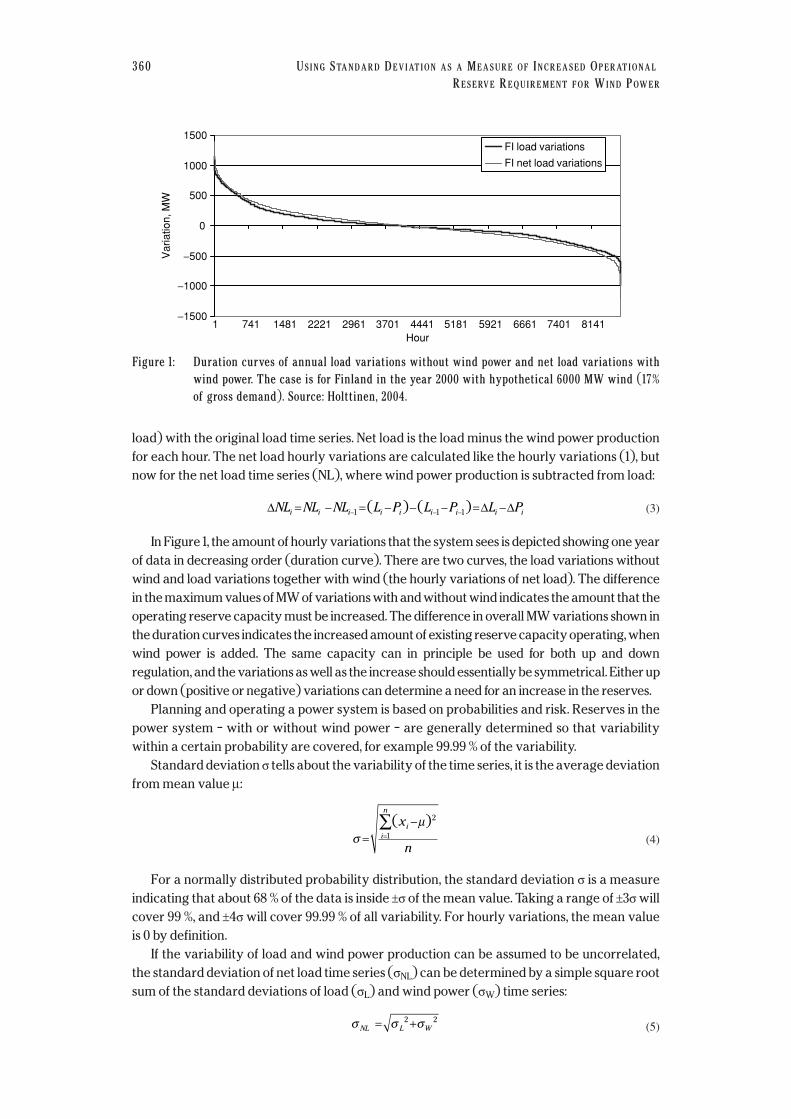
In Figure 1, the amount of hourly variations that the system sees is depicted showing one year
of data in decreasing order (duration curve). There are two curves, the load variations without
wind and load variations together with wind (the hourly variations of net load). The difference
in the maximum values of MW of variations with and without wind indicates the amount that the
operating reserve capacity must be increased. The difference in overall MW variations shown in
the duration curves indicates the increased amount of existing reserve capacity operating, when
wind power is added. The same capacity can in principle be used for both up and down
regulation, and the variations as well as the increase should essentially be symmetrical. Either up
or down (positive or negative) variations can determine a need for an increase in the reserves.
Planning and operating a power system is based on probabilities and risk. Reserves in the
power system – with or without wind power – are generally determined so that variability
within a certain probability are covered, for example 99.99 % of the variability.
Standard deviation σ tells about the variability of the time series, it is the average deviation
from mean value µ:
(4)
For a normally distributed probability distribution, the standard deviation σ is a measure
indicating that about 68 % of the data is inside ±σ of the mean value. Taking a range of ±3σ will
cover 99 %, and ±4σ will cover 99.99 % of all variability. For hourly variations, the mean value
is 0 by definition.
If the variability of load and wind power production can be assumed to be uncorrelated,
the standard deviation of net load time series (σNL) can be determined by a simple square root
sum of the standard deviations of load (σL) and wind power (σW) time series:
(5)σ σ σNL L W= +2 2
σµ
=−
=∑( )x
n
i
i
n2
1
∆ ∆ ∆NL NL NL L P L P L Pi i i i i i i i i= − = − − − = −− − −1 1 1( ) ( )
360 USING STANDARD DEVIATION AS A MEASURE OF INCREASED OPERATIONAL
RESERVE REQUIREMENT FOR WIND POWER
Figure 1: Duration curves of annual load variations without wind power and net load variations with
wind power. The case is for Finland in the year 2000 with hypothetical 6000 MW wind (17%
of gross demand). Source: Holttinen, 2004.
−1500
−1000
−500
0
500
1000
1500
1 741 1481 2221 2961 3701 4441 5181 5921 6661 7401 8141Hour
Var
iatio
n, M
W
FI load variations
FI net load variations
The hourly variability of wind power production and load do experience some correlation
in the data of some regions. Also, the distribution of the variations is not usually strictly a
normal distribution. However, formula (5) has been checked for several sets of data and it has
produced accurate results for the standard deviation of the net load (Holttinen, 2005).
Finally, the increase in the variability due to the wind can be formulated as the increase in
some multiple of σ, calculating the increase from σL to σNL using for example 4σ as the
confidence level covering most of the variability:
(6)
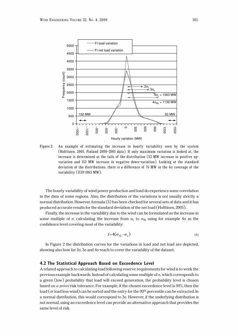
In Figure 2 the distribution curves for the variations in load and net load are depicted,
showing also how far 2σ, 3σ and 4σ reach to cover the variability of the dataset.
4.2 The Statistical Approach Based on Exceedence LevelA related approach to calculating load following reserve requirements for wind is to work the
previous example backwards. Instead of calculating some multiple of σ, which corresponds to
a given (low) probability that load will exceed generation, the probability level is chosen
based on a priori risk tolerance. For example, if the chosen exceedence level is 99%, then the
load (or load less wind) can be sorted and the entry for the 99th percentile can be extracted. In
a normal distribution, this would correspond to 3σ. However, if the underlying distribution is
not normal, using an exceedence level can provide an alternative approach that provides the
same level of risk.
I NL L= −4( )σ σ
WIND ENGINEERING VOLUME 32, NO. 4, 2008 361
Figure 2: An example of estimating the increase in hourly variability seen by the system
(Holttinen, 2005, Finland 2000–2001 data). If only maximum variation is looked at, the
increase is determined at the tails of the distribution (52 MW increase in positive up-
variation and 152 MW increase in negative down-variation). Looking at the standard
deviation of the distributions, there is a difference of 76 MW in the 4σ coverage of the
variability (1139-1063 MW).
0
500
1000
1500
2000
2500
3000
3500
4000
4500
5000
−1500
−1200
−900
−600
−300
0 300
600
900
1200
1500
Hourly variation (MW)
Fre
quen
cy (
coun
t)
FI load variation
FI net load variation
4σNL = 1139 MW
52 MW152 MW
2σL3σL
4σL = 1063 MW

To examine the reserve impact of wind, this approach can be easily done by (1) calculating
a given exceedence level (percentile) for load alone, (2) calculate the same exceedence level
(percentile) for the load net wind, and (3) comparing the incremental capacity of the two
calculations. An example from Minnesota in the United States will be shown in a later section
of this paper.
5. APPLYING SIGMA METHOD TO DIFFERENT TIME SCALES AND TIME SERIES5.1 Time Scales of Regulation and Load FollowingRegulating reserve must be available through the automatic generation control (AGC)
scheme and responds over time periods of up to several minutes. It is not uncommon for the
system operator to carry regulating reserves equal to ±5σ or ±6σ, where σ is the system
variability measured as standard deviation of the load variability.
However, over longer time scales it may be possible to obtain generator responses from
other sources, including non-AGC units that are spinning and synchronized, market
participants, or quick-start generation that is not spinning. In systems with significant run-of-
river hydro, the overall system variability will also be a function of the hydro variability over
the time scale of 10–60 minutes, in addition to load and wind forecast errors and sub-hourly
ramping. Some recent studies in the United States, for example (EnerNex, 2006; EnerNex, 2007
and Idaho Power, 2007) have used ± 2σ as the preferred metric to calculate load following
requirements for wind. This is based on the requirement (imposed by the North American
Electricity Reliability Corporation, NERC) that the minimum required score for control
performance standard 2 (CPS2) is 90%, which approximately corresponds to the normal
probability value for 2σ. Other U.S. studies have used ±3σ as the appropriate confidence
interval (GE Energy, 2007; Dragoon & Milligan, 2003; Milligan, 2003). A recent study
undertaken by GE Energy of the Ontario system used ±3σ and used a corresponding
exceedence analysis as a supplement (GE, 2006).
As more data and other methods for reserve requirement estimation emerge, it is
interesting to see how well the general assumptions of multiples of sigma used so far in the
studies reflect the increase in reserve requirement needs due to wind power.
5.2 Applying Sigma Method to Load Forecast or Load Variation Time SeriesRegulation and load following reserves are used as balancing services required after
generators have moved to follow energy price signals. Clearly, there is more residual left if
only hourly energy markets are available and less if there are five minute energy markets.
The physical power system sets energy market prices in order to move generators’ output
based on a short term forecast of expected load movements. The desire is to move the economic
units (units being dispatched to provide energy based on their cost or price) to the centre of the
expected load range and to simultaneously move the regulating units to the centre of their
response range. This positions them best to be able to respond to the next random load
movement.
When modelling the power system it would be best to either record the short term load
forecasts or to have sufficient information to enable creation of a short term load forecast to
position the economic generators. This is difficult because it involves either recording a great
deal of forecast data that most system operators do not currently record or it requires
duplicating their sophisticated load forecasting tools and having access to the large amount
of data that they themselves require.
If the forecasts are not available, an analysis technique provides a simple but excellent
proxy for short term forecasts. A rolling average of the load time-series can be used as a
362 USING STANDARD DEVIATION AS A MEASURE OF INCREASED OPERATIONAL
RESERVE REQUIREMENT FOR WIND POWER

forecast for the load-following component. This works (and is a good approximation of
reality) because short term load forecasts themselves are typically quite accurate. The
correct rolling average duration depends on the type of short-term energy market that is
available. If only hourly markets are available then a 60 minute rolling average is appropriate.
If a five minute energy market is operating then a five minute rolling average is appropriate
(Kirby & Hirst, 2000; Kirby & Hirst, 2001). It turns out that in practice with real power systems
the exact rolling average time interval is not important but the range is: there is little
difference between five and ten minute rolling averages but a large difference between five
and sixty minute rolling averages. In any event, using a rolling average to separate regulation
from load-following captures the full variability of the load. The technique simply segregates
that total variability into the two categories.
5.3 Wind DataIt is important to look at the representation of the wind data to describe the hourly variability
of large scale wind power production. The data needs to be upscaled to look for the future
impacts of large scale wind power. If too few time series of wind power plants are used,
upscaling the time series will also upscale the hourly variations, not taking into account the
smoothing effect of thousands of turbines at hundreds of sites. At some stage the smoothing
effect will saturate: adding more turbines/sites will not result in less variability (Holttinen
et al, 2007).
Large scale wind power production varies less the smaller the time step considered (Ernst,
1999). The results from a study for Northern Ireland suggest that at a 10% penetration, the
increase in hourly variability in the net load (load – wind power) is less than 2% of wind power
capacity, whereas the half-hourly data gives an increase of less than 1% of wind power
capacity (Persaud et al., 2000).
5.4 Varying Reserve Requirements Throughout The YearWhen wind is generating a small fraction of its rated output, it makes little sense to hold up-
capable load following reserves that would guard against a drop in wind of the same
magnitude as its rated output. Likewise, when wind generation is near maximum output,
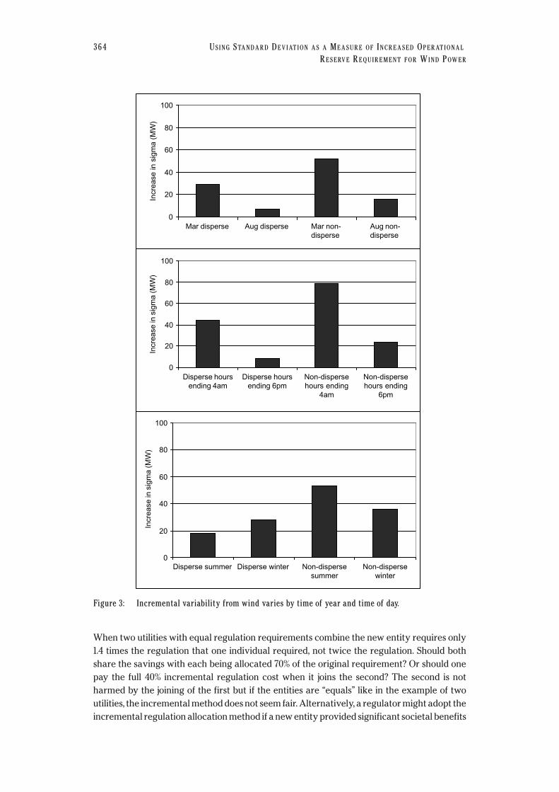
downward load following ability will depend on load levels, not wind. Figure 3 is taken from
(Krich & Milligan, 2005) and shows the incremental variability that wind adds to load in the
hourly time frame. The graphs separate a geographically disperse case (installed capacity
divided to three sites with equal amounts of wind power) from a non-dispersed case (same
amount of MW’s all at one site), and show various seasons, months and hours. It is clear from
the figure that incremental reserves that are induced by wind would not be constant
throughout the year. At least one recent integration study in the United States has explicitly
calculated this variable reserve, and will be discussed later in this paper in section of case
Minnesota.
5.5 Allocation MethodsThe incremental increase in reserve requirement due to wind power is often used as the
reserve requirement for wind power. Instead of allocating the simple addition to wind power
it is also possible to take the total reserve requirement and allocate that to both wind and loads
by alternative means. Selecting a variability allocation method is not exclusively a technical
matter. Individual load and/or generator variability is usually not highly correlated with the
variability of other loads and/or generators. When multiple individuals are aggregated
together the variability of the total is less than the sum of the variability of the individuals.
WIND ENGINEERING VOLUME 32, NO. 4, 2008 363
When two utilities with equal regulation requirements combine the new entity requires only
1.4 times the regulation that one individual required, not twice the regulation. Should both
share the savings with each being allocated 70% of the original requirement? Or should one
pay the full 40% incremental regulation cost when it joins the second? The second is not
harmed by the joining of the first but if the entities are “equals” like in the example of two
utilities, the incremental method does not seem fair. Alternatively, a regulator might adopt the
incremental regulation allocation method if a new entity provided significant societal benefits
364 USING STANDARD DEVIATION AS A MEASURE OF INCREASED OPERATIONAL
RESERVE REQUIREMENT FOR WIND POWER
Figure 3: Incremental variability from wind varies by time of year and time of day.
0
20
40
60
80
100
Mar disperse Aug disperse Mar non-disperse
Aug non-disperse
Incr
ease
in s
igm
a (M
W)
0
20
40
60
80
100
Disperse hoursending 4am
Disperse hoursending 6pm
Non-dispersehours ending
4am
Non-dispersehours ending
6pm
Incr
ease
in s
igm
a (M
W)
Disperse summer Disperse winter Non-dispersesummer
Non-dispersewinter
0
20
40
60
80
100
Incr
ease
in s
igm
a (M
W)

such as job creation (steel mills) or environmental benefits (wind generators). The rest of the
system would see no increase in regulation cost and the industrial plant or wind generator
would be interconnected at minimal cost.
Variability can be allocated based upon causation while accounting for the nonlinearity
(Kirby and Hirst, 2000). The allocation methodology is independent of the order in which
entities are added to the aggregation and independent of how many or few pieces the total is
split into. Individual variabilities can exhibit any amount of correlation. The total allocated
variability always equals the total system variability. Figure 3 illustrates the allocation
method graphically when two entities (A ad B) are combined. It is the correlation of the
individual with the total requirement that determines the allocation.
Numerical implementation of the allocation method, shown in equation 7, is
straightforward and can be done for as many or as few individual generators and loads as
desired. The allocated variability is then multiplied by the same factor that total variability
was multiplied by to determine the reserve requirement in MW.
(7)
Using this allocation method will increase the integration cost estimate for wind power. In
most power systems, different loads and production units do not pay different tariffs for the
regulation burden they pose to the system. As a result, some nonconforming loads which
impose much higher than average regulation burdens on the power system, pay for far less
regulation than they should. To date individual load allocation has not been implemented in a
tariff. Until the reserve requirements are allocated to individual loads and production units, it
is well justified by wind integration studies to calculate only the simple addition to reserve
requirements. Both methods result in full cost recovery for the utility.
6. CASE: MINNESOTA, USIn 2005 the Minnesota (US) legislature directed the Public Utilities Commission to analyse the
impact of a 20% renewable portfolio standard in the state. Under the assumption that most of
this renewable generation would come from wind, the PUC retained EnerNex Corp, who with
WindLogics, developed detailed chronological wind generation estimates and simulated the
Minnesota grid to determine the impact, and ultimately, the integration cost of wind.
6.1 Comparison of Exceedence Level and Sigma ApproachesTo provide a simple analysis of the relationship between the sigma approach and a statistical-
exceedence method, we obtained the hourly data from the study and analyzed it for this
paper. Figure 4 shows the data in graphical form.
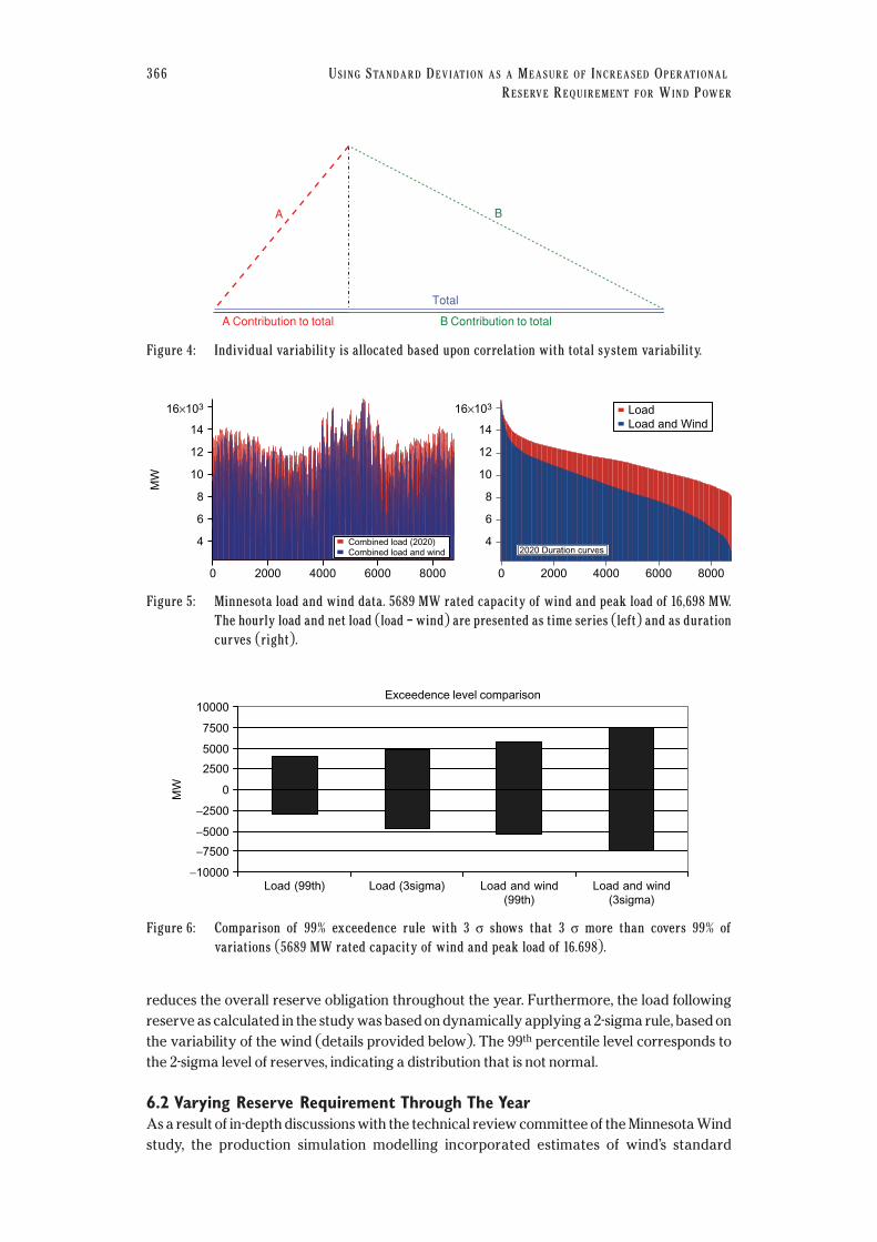
Using this data we calculated the exceedence level at 99% for load, and for load with wind. The
basis of the calculation was to investigate the 99th percentile of the variations in load compared
to load - wind. We then compared this with a 3σ rule. The results appear in Figure 5.
The results indicate that the number of sigmas that result in 99% exceedence is between
2.3–2.5, as indicated in Figure 6. The data in this discussion is taken from a 25% (energy) wind
penetration. The 3-sigma rule results in a very high reserve margin in the load following time
scale, 31–40% of wind rated capacity for a 2-sigma and 3-sigma rule, respectively. The 99th
percentile exceedence rule results in a 31% reserve. This is clearly much higher than other
results in this paper.
There are a few clarifying points that should be made. The reserve calculation in the
integration study from which the data was obtained utilized a variable reserve method that
AllocationA Total A Total A Tota= + − −( )/(σ σ σ σ2 2 2 2 ll )
WIND ENGINEERING VOLUME 32, NO. 4, 2008 365
reduces the overall reserve obligation throughout the year. Furthermore, the load following
reserve as calculated in the study was based on dynamically applying a 2-sigma rule, based on
the variability of the wind (details provided below). The 99th percentile level corresponds to
the 2-sigma level of reserves, indicating a distribution that is not normal.
6.2 Varying Reserve Requirement Through The YearAs a result of in-depth discussions with the technical review committee of the Minnesota Wind
study, the production simulation modelling incorporated estimates of wind’s standard
366 USING STANDARD DEVIATION AS A MEASURE OF INCREASED OPERATIONAL
RESERVE REQUIREMENT FOR WIND POWER
Figure 4: Individual variability is allocated based upon correlation with total system variability.
A Contribution to total B Contribution to total
B
Total
A
Figure 5: Minnesota load and wind data. 5689 MW rated capacity of wind and peak load of 16,698 MW.
The hourly load and net load (load – wind) are presented as time series (left) and as duration
curves (right).
MW
80006000400020000
2020 Duration curves
LoadLoad and Wind
16×103
14
12
10
8
6
4
16×103
14
12
10
8
6
4
MW
80006000400020000
Combined load (2020)Combined load and wind
Figure 6: Comparison of 99% exceedence rule with 3 σ shows that 3 σ more than covers 99% of
variations (5689 MW rated capacity of wind and peak load of 16.698).
Exceedence level comparison
−10000
−7500
−5000
−2500
0
2500
5000
7500
10000
Load (99th) Load (3sigma) Load and wind(99th)
Load and wind(3sigma)
MW

deviation to calculate variable operating reserve. The approach used is a variation of those
discussed in prior sections of this paper; instead of calculating a single multiple of sigma, this
approach used a dynamic approach that allowed the reserve level to be calculated based on
the amount of wind generation that was operating. EnerNex divided the chronological wind
generation into quintiles based on generation level, and then calculated the standard
deviation within each grouping. Based on the results, a variable operating reserve component
based on 2σ of the change in hourly wind generation was added geometrically (as root-sum-
squares process) to the production simulation modelling. Dividing the wind generation into
quintiles, the standard deviation for each quintile was calculated, and a series of quadratic
functions were estimated, one for each penetration level. The quadratic functions are based
on fitting the two-sigma changes in wind production for each quintile, Figure 8 shows the
quadratic functions and the respective curves for each of the wind penetration levels studied.
Figure 9 illustrates the relationship between the additional reserve imposed by wind and
the level of wind generation based on the quadratic formulas, and is adapted from the
WIND ENGINEERING VOLUME 32, NO. 4, 2008 367
Figure 7: Number of sigmas to achieve the reserve requirement of 99% exceedence level analysis, for
up-and down regulation needs.
Number of standard deviations for constantexceedence (99%)
−3.00
−2.00
−1.00
0.00
1.00
2.00
3.00
Load Load and wind
Num
ber
of s
igm
as
Figure 8: Reserve component based on the standard deviation of net-hour wind generation.
700
600
500
400
300
200
100
0
Add
ition
al r
eser
ve (
MW
)
6000500040003000200010000Wind generation in operating hour (MW)
f15(x) = 400 − [(x − 2000)^2] / 9000f20(x) = 550 − [(x − 2800)^2] / 15000f25(x) = 700 − [(x − 3500)^2] / 17500
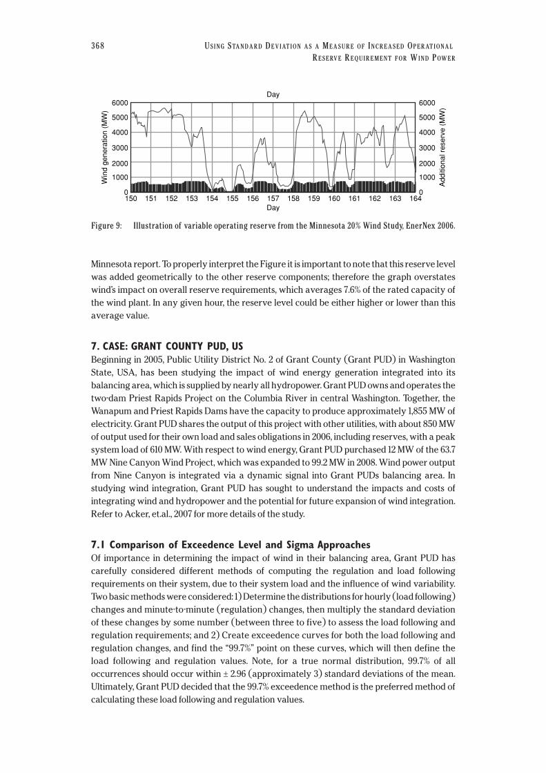
Minnesota report. To properly interpret the Figure it is important to note that this reserve level
was added geometrically to the other reserve components; therefore the graph overstates
wind’s impact on overall reserve requirements, which averages 7.6% of the rated capacity of
the wind plant. In any given hour, the reserve level could be either higher or lower than this
average value.
7. CASE: GRANT COUNTY PUD, USBeginning in 2005, Public Utility District No. 2 of Grant County (Grant PUD) in Washington
State, USA, has been studying the impact of wind energy generation integrated into its
balancing area, which is supplied by nearly all hydropower. Grant PUD owns and operates the
two-dam Priest Rapids Project on the Columbia River in central Washington. Together, the
Wanapum and Priest Rapids Dams have the capacity to produce approximately 1,855 MW of
electricity. Grant PUD shares the output of this project with other utilities, with about 850 MW
of output used for their own load and sales obligations in 2006, including reserves, with a peak
system load of 610 MW. With respect to wind energy, Grant PUD purchased 12 MW of the 63.7
MW Nine Canyon Wind Project, which was expanded to 99.2 MW in 2008. Wind power output
from Nine Canyon is integrated via a dynamic signal into Grant PUDs balancing area. In
studying wind integration, Grant PUD has sought to understand the impacts and costs of
integrating wind and hydropower and the potential for future expansion of wind integration.
Refer to Acker, et.al., 2007 for more details of the study.
7.1 Comparison of Exceedence Level and Sigma ApproachesOf importance in determining the impact of wind in their balancing area, Grant PUD has
carefully considered different methods of computing the regulation and load following
requirements on their system, due to their system load and the influence of wind variability.
Two basic methods were considered: 1) Determine the distributions for hourly (load following)
changes and minute-to-minute (regulation) changes, then multiply the standard deviation
of these changes by some number (between three to five) to assess the load following and
regulation requirements; and 2) Create exceedence curves for both the load following and
regulation changes, and find the “99.7%” point on these curves, which will then define the
load following and regulation values. Note, for a true normal distribution, 99.7% of all
occurrences should occur within ± 2.96 (approximately 3) standard deviations of the mean.
Ultimately, Grant PUD decided that the 99.7% exceedence method is the preferred method of
calculating these load following and regulation values.
368 USING STANDARD DEVIATION AS A MEASURE OF INCREASED OPERATIONAL
RESERVE REQUIREMENT FOR WIND POWER
Figure 9: Illustration of variable operating reserve from the Minnesota 20% Wind Study, EnerNex 2006.
6000
5000
4000
3000
2000
1000
Win
d ge
nera
tion
(MW
)
Add
ition
al r
eser
ve (
MW
)
0
6000
5000
4000
3000
2000
1000
0150 151 152 153 154 155 156 157 158 159 160 161 162 163 164
Day
Day

In computing the regulation and load following changes, a 10-minute rolling average of the
system load was created. The 1-minute regulation values were then computed by taking the
difference between the actual 1-minute system load and the 10-minute rolling average for data
from the first eleven months of 2006 (about 481,000 1-minute values; the twelfth month was not
available at the time of the analysis). The load following was computed by taking the signed
difference between the maximum and minimum value of the 10-minute rolling average during
each hour in the data set (about 8,000 1-hour changes). Other methods were considered for
defining the regulation and load following, such as using a 60-minute rolling average, but all
yielded similar results for the comparison to be made here.
Figure 10 shows a histogram of the regulation (1-minute) changes and its associated
exceedence curve. In creating the histogram and exceedence curves, Grant PUD’s 1-minute
system load was analyzed without wind (corresponding to 0 MW of wind) and netted (system
request minus wind power production) with 12, 63.7, and 150 MW of wind (1-minute generation
values). The actual output of the 63.7 MW Nine Canyon project was used in making these
calculations, and directly scaled to either 12 MW or 150 MW, which in both cases will distort the
actual variability of the wind output. For that reason, only the numerical results for the 63.7
MW case will be presented here (note that the system was actually run with 12 MW, and the
63.7 MW is a hypothetical case).
A summary of the results for the regulation and load following calculations are given in
Table 1, for the case of 63.7 MW of wind. This corresponds to a wind penetration level of
10.4%, based upon peak capacity (63.7 MW of wind divided by a peak system load in 2006
of 610 MW). The “Standard Deviation” and “99.7% Exceedence” columns shown in this
table provide the results for system load only (no wind), for the system load netted with
63.7 MW of wind, and the difference between the two. Shown in the “Multiples of Std. Dev.”
column is the number of times it is necessary to multiply the standard deviation value to
obtain the associated 99.7% exceedence value. As is demonstrated in these results, in order
to obtain the exceedence value, it is necessary to multiply the standard deviation values
by about 5.6 to obtain the regulation as determined by the exceedence value, and by about
3.4 to obtain the load following as determined by the exceedence value. Note the number
of multiples of standard deviations is rather insensitive to whether or not the wind is
included.
WIND ENGINEERING VOLUME 32, NO. 4, 2008 369
Table 1. Grant PUD results for standard deviation and exceedence value methods ofcomputing the load following and regulation requirements, for 63.7 MW of wind power,2006 data. Multiples of sigma indicate reserve requirement estimation from exceedencevalue results: 5.5–5.6 times sigma for regulation time scale and 3.3–3.4 times sigma for
load following time scale.
Standard Deviation 99.7% Exceedence Multiples of Std. Dev.Value
Load Load LoadRegulation Following Regulation Following Regulation Following
(MW) (MW) (MW) (MW) (MW) (MW)System load only 2.09 12.09 11.68 39.86 5.59 3.30
System load net 2.11 12.90 11.74 43.86 5.56 3.40
63.7 MW wind
Increase due to 0.02 0.81 0.06 4.00
wind

370 USING STANDARD DEVIATION AS A MEASURE OF INCREASED OPERATIONAL
RESERVE REQUIREMENT FOR WIND POWER
Figure 10: Regulation histogram (top) and exceedence curves (bottom) for Grant PUD 2006 system load
considering 0, 12, 63.7, and 150 MW of wind capacity.
<−16
−16
to −1
5
−16
to −1
4
−14
to −1
3
−13
to −1
2
−12
to −1
1
−11
to −1
0
−10
to −9
−9 to
−8
−8 to
−7
−7 to
−6
−6 to
−5
−5 to
−4
−4 to
−3
−3 to
−2
−2 to
−1
−1 to
00
to 11
to 22
to 33
to 44
to 55
to 66
to 77
to 88
to 9
9 to
10
10 to
11
11 to
12
12 to
13
13 to
14
14 to
15
15 to
16>
16
16
Regulation (10min rolling average)
0 MW12 MW63.7 MW150 MW
14
12
10
Fre
quen
cy (
%)
8
6
4
2
0
0MW12MW63.7MW150MW
Fre
quen
cy o
f reg
ulat
ion
(%)
100
90
80
70
60
50
40
30
20
10
010 20 30 40
Absolute regulation magnitude (MW)50 60 70 800
Percentage of regulation (GCPUD method) exceeding magnitude of X

WIND ENGINEERING VOLUME 32, NO. 4, 2008 371
8. CASE: FINLAND AND NORDELHourly wind power production time series from 4 Nordic countries were collected for a PhD
study on impacts of wind power on the Nordic power system (Holttinen, 2004). Data for hourly
wind power production was available from 21 sites in Finland, 6 sites in Sweden, 6-12 sites in
Norway and the aggregated total production of hundreds of sites in Denmark West and East. A
Nordic data set was formed from the data sets of the 4 countries: Denmark, Sweden, Norway and
Finland. The total electricity consumption from the countries, also as hourly time series, was
obtained from the same period as wind power production data: years 2000 to 2002. Data is
analysed in more detail and the data handling procedure for wind power time series is described
in more detail in (Holttinen, 2005). The Nordic wind power production time series was made in
two ways: a simple average of the percentage of capacity production of the 4 countries and a
more concentrated dataset “Nordic 2010” where half of the wind power capacity is in Denmark.
8.1 Comparing the Sigma Approach with Forecast DataSimple analysis based on the increase in 4σ variability assumes that the hourly variations of
both load and wind power production are unexpected. However, as the load with its clear
diurnal pattern is easier to forecast than wind power production, this should be taken into
account when analysing the increase in operating reserve requirement due to wind power
(Milligan, 2003).
For wind power, the production an hour ahead can be reasonably well forecasted by
persistence, that is, taking the production level at hour i-1 for the predicted value at hour i . This
actually results in using the hourly variation as used in previous sections as a measure of
forecast error of wind power production. Short term prediction tools can improve this to some
extent, taking into account the forecasted trend of wind speeds in the area, as well as time
series techniques that are proven to work quite well for some hours ahead (Giebel et al, 2003).
The persistence method therefore produces a conservative estimate for hour-ahead wind
power production.
In a case study for Finland, year 2001 load data was carried out to estimate load forecasts.
A model at VTT Technical Research Centre of Finland was used, based on calendar days of
loads (from year 2000 data) and temperature (Koreneff et al, 1998 and 2000). The mean
absolute error, hour ahead, was 0.7 % of peak load. The forecast error for the load was then
compared to wind power variations. The standard deviation of forecast error was 123 MW
(1% of peak load). This compares with 267 MW for the load hourly variations, so this method
assumes that about half of the variability in load can be predicted.
The results when using load forecast error instead of the hourly variation of load show that
the results based on the simple hourly variations from load and wind power time series, should
be doubled if no hour ahead wind forecast is assumed. Applying this to the results of Nordic
and Denmark area gives the results presented in Figure 11 and Table 2.
The results show that when the penetration of wind power in the system increases, an
increasing amount needs to be allocated for operating reserve. For a single country the
increase in reserve requirements can range 2.5–4% of the installed wind power capacity at 10%
penetration. The effect of wind power is nearly double in Finland compared to that for
Denmark. This is mainly due to the low initial load variability in Finland. When the Nordic
system works without bottlenecks of transmission the impact of wind power becomes
significant at 10% penetration level, when the increase in reserve requirement due to wind
power is about 2% of installed wind power capacity or 310–420 MW. At a high wind power
penetration of 20%, the increase is already about 4% of wind power capacity or 1200–1600 MW.
The range is for a more-or-less concentrated wind power capacity in the Nordic countries.
The estimation is based on hourly wind power data from a 3-year-period in which the wind
resource was less than average. This may underestimate the true variability. For the Danish
data, the error was estimated to be on the order of 5%, and it has been added to the results in
Figure 11 and in the last section of Table 2.
The reserve requirements due to load and wind ramping within the hour has been
assumed to be included in the reserve requirements calculated by the sigma approach.
9. CASE: SWEDENThe Swedish wind power series were obtained as a result of the project reported in
(Magnusson et al, 2004). The so called synthetic time series are based on a database with
relevant climatological parameters for the period 1992–2001 and cover the production of 56
wind farms based on locations throughout Sweden. About 40% of the wind farms are located
at sea and each has an installed capacity between 50 and 300 MW. These account for 75% of
372 USING STANDARD DEVIATION AS A MEASURE OF INCREASED OPERATIONAL
RESERVE REQUIREMENT FOR WIND POWER
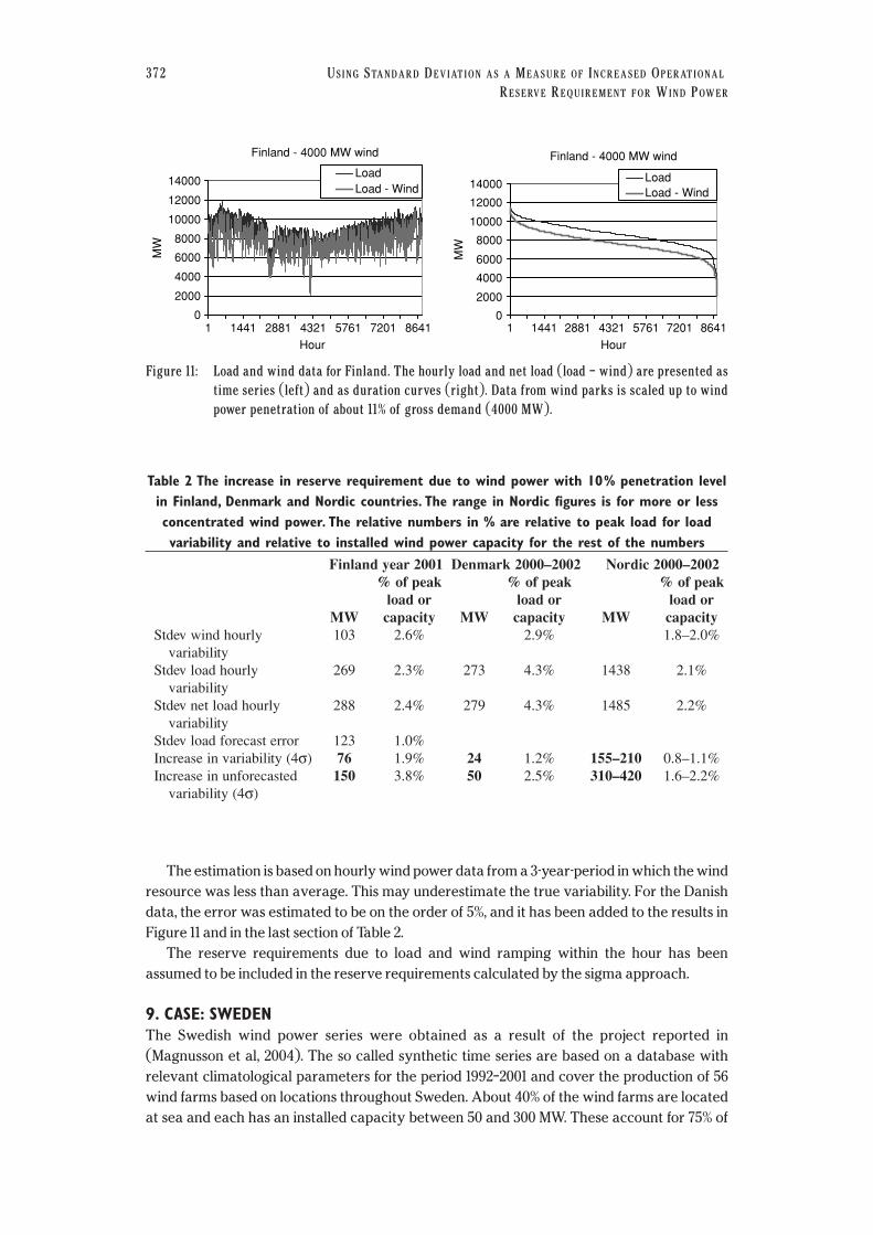
Figure 11: Load and wind data for Finland. The hourly load and net load (load – wind) are presented as
time series (left) and as duration curves (right). Data from wind parks is scaled up to wind
power penetration of about 11% of gross demand (4000 MW).
Finland - 4000 MW wind
0
2000
4000
6000
8000
10000
12000
14000
Hour
MW
LoadLoad - Wind
1 1441 2881 4321 5761 7201 8641
Finland - 4000 MW wind
0
2000
4000
6000
8000
10000
12000
14000
MW
LoadLoad - Wind
1 1441 2881 4321 5761 7201 8641
Hour
Table 2 The increase in reserve requirement due to wind power with 10% penetration levelin Finland, Denmark and Nordic countries. The range in Nordic figures is for more or lessconcentrated wind power. The relative numbers in % are relative to peak load for loadvariability and relative to installed wind power capacity for the rest of the numbers
Finland year 2001 Denmark 2000–2002 Nordic 2000–2002% of peak % of peak % of peak
load or load or load orMW capacity MW capacity MW capacity
Stdev wind hourly 103 2.6% 2.9% 1.8–2.0%variability
Stdev load hourly 269 2.3% 273 4.3% 1438 2.1%variability
Stdev net load hourly 288 2.4% 279 4.3% 1485 2.2%variability
Stdev load forecast error 123 1.0%Increase in variability (4σ) 76 1.9% 24 1.2% 155–210 0.8–1.1%Increase in unforecasted 150 3.8% 50 2.5% 310–420 1.6–2.2%
variability (4σ)

the total capacity installed. In total, the assumed installed wind power capacity was 4000 MW
corresponding to 10 TWh/a of generation.
The load forecast error is calculated from a load database received from Swedish TSO
Svenska Kraftnät for the years 2002, 2003, and 2004.
9.1 Comparing Results for Load Variations and Load Forecast Time SeriesThe power system reserve requirements for different wind power scenarios based on hourly
analysis has been calculated in (Axelsson et al, 2005). The statistical method based on 4σ analysis
of net load variability was compared with the statistical method including forecast errors.
4000 MW wind power was simulated according to the data from (Magnusson et al, 2004). The
results for the different methods of calculating the additional variability in net load in Sweden
(increase in reserve requirement) caused by 4000 MW wind power are presented in Table 3.
For wind power two cases for the forecast were used – the persistence an hour ahead
(which means no forecast – case load forecast only) and an assumed improvement to
persistence by forecasting (case load and wind forecast). The load forecast error is calculated
from a load database received from TSO Svenska Kraftnät for the years 2002, 2003, and 2004.
Analysis of this data shows that both the variability of the load in Sweden as well as forecast
error is larger than in Finland. Standard deviation of hourly load variability in Sweden is 2.4%
and forecast error is 1.4% (an improvement by over 40%). The difference between Sweden and
Finland can be explained by different proportions of the types of consumers with domination
of industrial load in Finland.
At the time of implementation of the study presented in (Axelsson et al, 2005) the main
scenario was that most of wind power in future would be implemented offshore and in the
southern part of the country. However, recent activity indicates more rapid development of
wind power on land both in Southern Sweden and in the North. The new estimations are that
about 50% of wind power will be located in the South and 50% in the North. Similarly it is
believed that about 50% of installed wind power capacity will be on land and 50% offshore.
This will reduce the variability compared with the calculations reported in (Axelsson et al,
2005). The standard deviation of hourly wind variability would decrease in the 4000 MW case
from 73 MW to 58 MW (1.4% of installed wind power capacity) (Table 3). Combining wind
variability with load variability results in a net load variability standard deviation of 578 MW
WIND ENGINEERING VOLUME 32, NO. 4, 2008 373
Figure 12: Increase in hourly load following requirement for wind power, calculated from the standard
deviation values of load and wind power production from years 2000–2002. Increase is
relative to installed wind power capacity.
0%
1%
2%
3%
4%
5%
6%
7%
8%
0% 5% 10% 15% 20% 25%Wind power penetration (% of gross demand)
Incr
ease
in r
eser
ve r
equi
rem
ent
(% o
f ins
talle
d w
ind
capa
city
)
Finland
Denmark
Nordic
Nordic 2010

(2.5%), which results in a 12 MW increase in 4σ variability due to wind power compared with
the 19 MW calculated before.
If instead of load variability the load forecast error is used, the corresponding standard
deviation of load forecast error will be 334 MW (1.3%) resulting in a 20 MW increase in 4σvariability as compared with 12 MW calculated before. This means that a 67% increase in the
result based on load variability will result, when taking into account the better predictability
of load. However, taking into account that wind can also be predicted hour ahead, the result is
close to the first calculation with simple load and wind variability.
10. SUMMARY OF THE CASE STUDY RESULTS AND CONCLUSIONSThe variability inherent of wind power production will require increased flexibility in the
power system when a significant amount of load is covered by wind power. Standard
deviation of variability for load and net load (load minus wind power production) has been
used when estimating the effect of wind power on the short term reserves of the power
374 USING STANDARD DEVIATION AS A MEASURE OF INCREASED OPERATIONAL
RESERVE REQUIREMENT FOR WIND POWER
Table 3 Summary of results for the different methods calculating the need for additionalreserves in Sweden for 4000 MW wind (6.6% penetration).Peak load 25800 MW has beenused for load and net load relative figures. Hourly analysis. The relative numbers in % arerelative to peak load for load variability and relative to installed wind power capacity for
the rest of the numbers4000 MW (50% offshore,
Wind power (MW) 4000 MW (70% offshore) more dispersed wind)% of peak load % of peak load
MW or wind capacity MW or wind capacityStdev wind power hourly 73 1.8% 58 1.5%
variabilityStdev load hourly 575 2.2% 575 2.2%
variability Stdev net load hourly 579 2.2% 578 2.2%
variability Stdev load forecast error 339* 1.3% 339* 1.3%Increase in variability (4σ) 19 0.5% 12 0.3%Increase in forecast error 31 0.8% 20 0.5%
variability (4 σ), load forecast only
Increase in forecast error 20 0.5% 13 0.3%variability (4 σ), loadand wind forecast
*The load forecast error is calculated from load database for the years 2002, 2003 and 2004 and not 1992 to 2001.
MW
1 1001 2001 3001 4001 5001 6001 7001 80010
5000
10000
15000
20000
25000
30000
LoadLoad and wind
1 1001 2001 3001 4001 5001 6001 7001 80010
5000
10000
15000
20000
25000
30000
MW
LoadLoad and wind
Figure 13: Load and wind data for Sweden (4000 MW wind installed). The hourly load and net load (load –
wind) are presented as time series (left) and as duration curves (right).

system. This method is straightforward and easy to use when time-series data on wind
power and load exist. Net load variability compared to load variability gives an estimate for
the needs of the system to react to large scale wind power. A statistical approach using the
standard deviation (σ) values gives estimates for the range of variability, for example
taking ±4σ as the range will cover most variations (99.99 % of all variations are inside this
range). So far, the multiple of sigmas has been on the order of 6σ for regulation reserves,
and in the range of 2-3σ for load following reserves. In this paper the sigma approach has
been compared with other methods. In this study, the incremental changes to the system
due to wind power were estimated for two cases in the US and the Nordic countries.
Minnesota results for a 25% (energy) wind penetration (34 % of peak load) show that the
dynamic reserve requirements average 7.6% of installed wind power capacity. The 99th
percentile exceedence rule results in a 31% reserve. This is clearly much higher than other
results in this paper, or in the international comparison (Holttinen et al, 2007).
Grant County results for a wind penetration level of 10.4% of peak load (63.7 MW of wind
divided by a peak system load in 2006 of 610 MW) show an increase in reserve requirement of
0.1% of wind power capacity at regulation time scale (minutes) and 6.3% of wind power
capacity at load following time scale (10 minutes), using an exceedence level 99.7%.
The Nordic countries results at 10% penetration (of electrical energy) show that for a single
country the increase in reserve requirements can range 2.5–4% of the installed wind power
capacity. When the Nordic system works without bottlenecks of transmission the increase in
reserve requirement due to wind power is about 2% of installed wind power capacity. At a high
wind power penetration of 20%, the increase is about 4% of wind power capacity. For Sweden
with a 6.6% penetration level (of electrical energy), the increase in reserve requirement is
0.5–0.8 % of installed wind power capacity.
The results of studies for different countries show that the percentage of reserve
requirements related to the installed wind power capacity varies greatly between different
systems. The results from US show higher reserve requirement estimates than the results
from the Nordic countries. The effect of wind power variability is higher in Finland than in
Denmark and Sweden. This is due to the following two main reasons: load variability in
Finland is lower than in Sweden or Denmark and wind power variability in Denmark and in
Sweden is less than in Finland. In Sweden, wind power is allocated across a larger
geographical area, which leads to more smoothing effect for wind power’s variability.
The results from US indicate that in the load following time scale the number of sigmas that
result in 99% exceedence is between 2.3-2.5 and the number of sigmas for 99.7 % exceedence is 3.4.
For regulation time scale the number of sigmas for 99.7 % exceedence is 5.6.
The estimates of increase in variability do not take into account the fact that the variability
is easier to predict for the load than for wind power production. The results from the Nordic
countries indicate that the number of sigmas should be increased by 67–100 % if better load
predictability is taken into account (combining hourly wind variability with load forecast
errors).
As more data and other methods for reserve requirement estimation emerge, it is
interesting to see how well the general assumptions of multiples of sigma used so far in the
studies reflect the increase in reserve requirement needs due to wind power.
ACKNOWLEDGEMENTSThe authors wish to express their gratitude to the wind power producers that have given
hourly production data from their wind park as well as all data received from the refereed
studies to make more detailed calculations.
WIND ENGINEERING VOLUME 32, NO. 4, 2008 375

REFERENCESAcker, T., Buecher, J., Knitter, K., and K. Conway. Impacts of Integrating Wind Power into the
Grant County PUD Balancing Area. Windpower 2007 Conference Proceedings (CD-ROM), 4–6
June 2007, Los Angeles, California.
Axelsson, U., Murray, R., Neimane, V., 2005. “4000 MW wind power: Impact on regulation and
reserve requirements”, Elforsk report 05:19, September 2005.
Dragoon, K., Milligan, M., 2003. Assessing Wind Integration Costs with Dispatch Models: A Case
Study of PacifiCorp. Windpower 2003 Conference Proceedings (CD-ROM), 18–21 May 2003,
Austin, Texas. Proceedings Sponsored by SPS, Specialized Power Systems, Inc.. Washington,
DC: American Wind Energy Association; Omni Press 13 pp.; NREL Report No. CP-500-38580.
Available at http://www.nrel.gov/publications/
EnerNex Corporation, 2006. Final Report – 2006 Minnesota Wind Integration Study. Minnesota
Public Utilities Commission. Available at http://www.uwig.org/windrpt_ vol%201.pdf.
EnerNex Corporation. 2007. Final Report - Avista Corporation Wind Integration Study. Avista
Utilities. Available at http://www.uwig.org/AvistaWindIntegrationStudy.pdf.
Ernst, B, 1999. Analysis of wind power ancillary services characteristics with German 250 MW
wind data. 38 pp.; NREL Report No. TP-500-26969 available at http://www.nrel.gov/publications/
GE, 2006. Ontario Wind Integration Study. Final Report to: Ontario Power Authority (OPA),
Independent Electricity System Operator (IESO) and Canadian Wind Energy Association
(CanWEA). Available at http://www.uwig.org/OPA-Report-200610-1.pdf.
GE Energy, 2007. Californian Intermittency Analysis. http://www.uwig.org/CEC-500-2007-081-
APA.pdf Giebel, G, Brownsword, R, Kariniotakis, G, 2003. The State-of-the-Art in Short-Term
Forecasting. Report for EU R&D Project “Development of a Next Generation Wind Resource
Forecasting System for the Large-Scale Integration of Onshore and Offshore Wind Farms”
ANEMOS. Available at http://anemos.cma.fr
General Electric and AWS Scientific/TrueWind solutions, 2007. New York State ERDA study.
http://www.nyserda.org/rps/draftwindreport.pdf
Holttinen, H., 2004. The impact of large scale wind power production on the Nordic electricity
system. VTT Publications 554. VTT Processes, Espoo., 2004. 82 p. + app. 111 p. Available at
http://www.vtt.fi/inf/pdf/publications/2004/P554.pdf
Holttinen, H., 2005a. Hourly wind power variations in the Nordic countries. Wind Energy. Vol.
8 (2005) No: 2, 173–195.
Holttinen, H., 2005b. Impact of hourly wind power variations on the system operation in the
Nordic countries. Wind Energy. Vol. 8 (2005) No: 2, 197–218.
Holttinen, H., Lemström, B., Meibom, P., Bindner, H., Orths, A., vanHulle, F., Ensslin, C., Hofmann,
L., Winter, W., Tuohy, A., O’Malley, M., Smith, P., Pierik, J, Tande, J. O., Estanqueiro, A., Ricardo,
J., Gomez, E., Söder, L., Strbac, G., Shakoor, A., Smith, J. C. Parsons, B., Milligan, M., Wan, Y., 2007.
Design and operation of power systems with large amounts of wind power. State-of-the-art
report. VTT, Espoo. 119 p. + app.25 p. VTT Working Papers : 82 http://www.vtt.fi/inf/pdf/
workingpapers/2007/W82.pdf
Idaho Power Corporation, 2007. Operational Impacts of Integrating Wind Generation into
Idaho Power’s Existing Resource Portfolio. Available at http://www.idahopower.com/pdfs/
energycenter/wind/windIntegrationstudy.pdf
Kirby, B., Hirst, E., 2000. Customer-specific metrics for the regulation and load following ancillary
services. ORNL/CON-474, Oak Ridge National Laboratory, Oak Ridge TN, January 2000.
376 USING STANDARD DEVIATION AS A MEASURE OF INCREASED OPERATIONAL
RESERVE REQUIREMENT FOR WIND POWER

Kirby, B., Hirst E. 2001, Using Five-Minute Data to Allocate Load-Following and Regulation
Requirements Among Individual Customers, ORNL/TM-2001-13, Oak Ridge National
Laboratory, Oak Ridge TN, January
Koreneff, G., Seppälä, A., Lehtonen, M., Kekkonen, V., Laitinen, E., Häkli, J., Antila, E., 1998.
Electricity spot price forecasting as a part of energy management in de-regulated power
market. Proceedings of EMPD ‘98. 1998 International Conference on Energy Management and
Power Delivery. Singapore, 3–5 March 1998. Vol. 1. IEEE. pp 223–228.
Krich, A, Milligan, M, 2005. The Impact of Wind Energy on Hourly Load Following
Requirements: An Hourly and Seasonal Analysis. Proceedings of Windpower 2005, Denver,
Colorado USA. CD-ROM. Available at http://www.nrel.gov/docs/fy05osti/ 38061.pdf.
Koreneff, G., Kekkonen, V., 2000. Distribution Energy Management (DEM) Systems and
Management of Commercial Balance. NORDAC 2000 -Nordic Distribution Automation
Conference. Stjördal 22–23 May 2000. Trondheim, DEFU in Denmark; VTT Energy; SINTEF
Energy Research; Elforsk, 2000. 10 p.
Kristoffersen, J. R., Christiansen, P., Hedevang, A., 2002. The wind farm main controller and the
remote control system in the Horns Rev offshore wind farm. Proceedings of Global Wind
Power Conference GWPC’02 Paris.
Magnusson, M., Krieg, R., Nord, M., Bergström, H., 2004. “Effektvariationer av vindkraft”,
Elforsk report 04:34, December 2004.
Milligan, M., 2003. Wind power plants and system operation in the hourly time domain.
Proceedings of Windpower 2003 conference, May 18–21, 2003 Austin, Texas, USA. NREL/CP-
500-33955 available at http://www.nrel.gov/publications/
Milligan, M. and Kirby, B. 2007. The Impact of Balancing Areas Size, Obligation Sharing, and
Ramping Capability, Proceedings of the WindPower 2007 Conference, June 3–5, 2007. Los
Angeles, CA, USA. NREL-CP-500-41809 available at http://www.nrel.gov/docs/
fy07osti/41809.pdf.
Persaud, S., Fox, B., Flynn, D., 2000. Modelling the impact of wind power fluctuations on the load
following capability of an isolated thermal power system. Wind Engineering (24) no 6. pp. 399–415.
Söder, L., 1999. Wind energy impact on the energy reliability of a hydro-thermal power system
in a deregulated market. In Proceedings of Power Systems Computation Conference, June
28–July 2, 1999, Trondheim, Norway.
WIND ENGINEERING VOLUME 32, NO. 4, 2008 377

Top Related
Copyright © 2022 FDOKUMEN

