


Bahasa
Halaman
Hukum

UNSTABLE SHIP MOTIONS
APLIED ON SHIP-WEATHER
ROUTING ALGORITHM
SIMROUTEv2
Bachelor’s Thesis
by
Lluís Basiana Ribera B.Sc
A thesis submitted in fulfilment of the requirements for the
degree of
Nautical Science and Maritime Transport
Department of Nautical Sciences and Engineering
Facultat de Nàutica de Barcelona
Universitat Politècnica de Catalunya
Barcelona
Submitted May 2018


Abstract
Some combinations of wave length and wave height under certain operational conditions
may lead to dangerous unstable motions for ships in accordance with the IS Code. The
susceptibility of a ship to dangerous phenomenon will depend on the stability parameters,
ship speed, hull shape and ship size. This signifies that the vulnerability to dangerous
responses, including capsizing, and its probability of occurrence in a singular sea state
may differ for each ship. During navigation periods these unstable motions are able to be
encountered, which may lead to a cargo or equipment damage and the unsafety of the
persons on board. The main reason for these causes is rarely known and currently there
are just few work such as the International Maritime Organization guidelines which tries
to ensure adequate dynamic stability (IMO, MSC.1/Circ.1228, 2007).
Ship routing systems are gaining importance in the maritime sector as the use of these
systems can lead to the reduction of fuel usage and reduce costs. Therefore, a mitigation
of carbon emissions and improvement of maritime safety happens due to the avoidance
of bad weather conditions. The implementation of pathfinding algorithms to determine
the optimal ship routing has been widely used for transoceanic distances. However, the
evaluation of short distance routes with ship-weather routing algorithms is still scarce,
due to the low spatial resolution of wave fields.
Mixing both concepts, that is to say, implementing the ship routing system with common
unstable motions makes the algorithm more complete and useful than it was. Thus, equip-
ping ships with these systems will be profitable for the officers because they will be able
to modify the stablished route or, at least, alter the course depending on the danger faced.
Results derived from such calculations should only be regarded as a supporting tool dur-
ing the decision-making process.
SIMROUTEv2 was developed to obtain the optimal route and the minimum distance
route recovered from the pathfinding algorithm A* (Grifoll et al., 2016). This system was
based on the inclusion of the added resistance by waves on the vessel, the impact of which
is significant in terms of time. Ship routing analysis was studied on four relative routes
related to five ports in the Western Mediterranean Sea, paying attention to the Short Sea

Shipping activities and the Ro-Pax and Ro-Ro services, being both of them the most fre-
quently performed in the aforementioned area (Basiana et al., 2017).
This project implements safety restrictions for avoiding broaching/surf-riding and para-
metric rolling according to the guidelines of the International Maritime Organization
(IMO circular no. 1228) in the SIMROUTEv2 algorithm. The expected output will be the
shortest route in terms of time and safety according to IMO guidelines for preventing
these aforementioned unstable motions. The methodology of the unstable motions imple-
mentation of this project is based on wave direction, peak wave period, encountered wave
period and the type of the vessel in terms of speed, length and the natural rolling period.
The work establishes the basis of further development in routes optimization utilized in
comparatively short-distances and its systematic use in the Short Sea Shipping maritime
industry and also in some other investigations of the unstable motions.
Keywords. Unstable motions, broaching, surf-riding, parametric rolling, ship routing,
Short Sea Shipping, wave models, safety navigation.
Figure 1: Minimum distance route (a) and Optimal route (b) from
Barcelona to Oran on 21/01/2017.
Estimated Time Departure (ETD): 20h. Initial speed: 22.6kn. Color
bar represents wave height. Source: Basiana et al. (2017)

Acknowledgements
The writing and completion of this Dissertation would not have been possible without the
assistance, the guidance and the support of a few people. I would like to show my grati-
tude to the following:
Clara Borén Altés, my supervisor in Universitat Politècnica de Catalunya, who
helped me since the first day, aiding and advising me throughout my project. She
provided guidance for all chapters found within this dissertation
Manel Grifoll Colls, my second supervisor, who helped me with the implementa-
tion of the unstable motions in the algorithm SIMROUTEv2
Marcel·la Castells Sanabra, an assistant professor investigating in Panama, who
provided me different papers and specific information related on the chapters of
this contribution
Maria Àngela Grau Gotes, an assistant professor and mathematician, who guided
me with the Matlab program
Charo Piera Lluch, the librarian of the Barcelona School of Nautical Studies of,
who helped me to find different books related on this work
My parents (Lourdes Ribera and Lluís Basiana). Thank you for always wanting
the best for me. Your love, concern, care, interest and trust has made me a stronger
person
My grandmother Teresa Mestres Marcet for taking care of me every single day of
my life and for enriching me with knowledge and moral courage

Table of content
LIST OF FIGURES ........................................................................................................ 7
LIST OF TABLES ........................................................................................................ 10
INTRODUCTION ........................................................................................................ 11
BACKGROUND AND LITERATURE ...................................................................... 12
AIMS AND OBJECTIVES .......................................................................................... 16
MAIN OBJECTIVE ......................................................................................................... 16
SPECIFIC OBJECTIVES ................................................................................................... 16
METHODOLOGY ....................................................................................................... 17
1. GENERAL MOTIONS OF A SHIP ....................................................................... 20
1.1. STABLE MOTIONS .................................................................................................. 20
1.1.1. Yaw ............................................................................................................... 21
1.1.2. Sway .............................................................................................................. 22
1.1.3. Surge ............................................................................................................. 23
1.1.4. Heave ............................................................................................................ 23
1.1.5. Pitch .............................................................................................................. 24
1.1.6. Roll ............................................................................................................... 25
1.2. UNSTABLE MOTIONS ............................................................................................. 26
1.2.1. Surf riding/Broaching ................................................................................... 26
1.2.2. Parametric rolling ........................................................................................ 29
1.2.3. Synchronous rolling ...................................................................................... 33
1.2.4. Slamming ...................................................................................................... 35
1.2.5. Green Water ................................................................................................. 36
2. UNSTABLE MOTIONS PARAMETERS ............................................................. 38
2.1. SURF-RIDING/BROACHING PARAMETERS .............................................................. 39
2.2. PARAMETRIC ROLLING PARAMETERS .................................................................... 40
3. SIMROUTEV2 ......................................................................................................... 44
3.1. BASIS AND ALGORITHM ........................................................................................ 44
3.2. WAVES ................................................................................................................. 46
3.3. COMMANDOS ........................................................................................................ 49
4. RESULTS .................................................................................................................. 51
4.1. CONVENTIONAL SHIP (21.5 KNOTS) ...................................................................... 53
4.2. FAST SHIP (28 KNOTS) .......................................................................................... 59
4.3. HIGH SPEED CRAFT (40 KNOTS) ............................................................................ 65
5. CONCLUSIONS ....................................................................................................... 71
6. REFERENCES ......................................................................................................... 73
7. FIGURE REFERENCES ......................................................................................... 77
8. TABLE REFERENCES ........................................................................................... 81
APPENDIXES 1. CODE IMPLEMENTATION ....................................................... 82
7
List of figures
FIGURE 1: MINIMUM DISTANCE ROUTE (A) AND OPTIMAL ROUTE (B) FROM BARCELONA
TO ORAN ON 21/01/2017. .......................................................................................... 9
FIGURE 2: APL CHINA ACCIDENT. SOURCE: THE LAW OFFICES OF COUNTRYMAN &
MCDANIEL (1998) ................................................................................................... 12
FIGURE 3: SIX FREEDOMS OF A SHIP’S MOTION. SOURCE: CLARK (2005) ........................ 20
FIGURE 4: YAW MOTION. SOURCE: CLARK (2005) ......................................................... 21
FIGURE 5: SWAY MOTION. SOURCE: CLARK (2005) ........................................................ 22
FIGURE 6: WAVE CYCLE AND SHIP POSITIONS. SOURCE: OWN ELABORATION ................. 22
FIGURE 7: SURGE MOTION. SOURCE: CLARK (2005) ....................................................... 23
FIGURE 8: HEAVE MOTION. SOURCE: CLARK (2005) ...................................................... 23
FIGURE 9: PITCH MOTION. SOURCE: CLARK (2005) ........................................................ 24
FIGURE 10: ROLL MOTION. SOURCE: CLARK (2005) ....................................................... 25
FIGURE 11: SIMULATION OF SURF-RIDING. SOURCE: UMEDA (2015) .............................. 27
FIGURE 12: THE RISK OF BROACHING IN HEAVY FOLLOWING SEAS. SOURCE: CLARK
(2005) ..................................................................................................................... 28
FIGURE 13: DANGEROUS SURF-RIDING ZONE. SOURCE: IMO, MSC.1/CIRC.1228 (2007)
................................................................................................................................ 29
FIGURE 14: PARAMETRIC ROLLING OF A FINE LINED HULL WITH A FULL STERN. SOURCE:
CLARK (2005) ......................................................................................................... 30
FIGURE 15: PARAMETRIC ROLLING ON A CONTAINER VESSEL. SOURCE: BARRASS &
DERRETT (2012) ...................................................................................................... 31
FIGURE 16: RISK OF SUCCESSIVE HIGH WAVE ATTACK IN FOLLOWING AND QUARTERING
SEAS. SOURCE: IMO, MSC.1/CIRC.1228 (2007) ..................................................... 33
FIGURE 17: TRANSVERSE WAVE PERIOD LESS THAN THE NATURAL ROLL PERIOD BEAM
SEA. SOURCE: CLARK (2005) ................................................................................... 34
FIGURE 18: TRANSVERSE WAVE PERIOD EQUAL TO THE NATURAL ROLL PERIOD BEAM SEA.
SOURCE: CLARK (2005) ........................................................................................... 34
FIGURE 19: TRANSVERSE WAVE PERIOD GREATER THAN THE NATURAL ROLL PERIOD
BEAM SEA. SOURCE: CLARK (2005) ......................................................................... 35
FIGURE 20: SLAMMING. SOURCE: ABADÍA DIGITAL (2013) ............................................ 36
FIGURE 21: GREEN WATER PHENOMENON. SOURCE: PETERSEN (1997) .......................... 36
FIGURE 22: DETERMINATION OF THE PERIOD OF ENCOUNTER TE. SOURCE: IMO,
MSC.1/CIRC.1228 (2007) ....................................................................................... 41
FIGURE 23: REPRESENTATION OF A PEAK WAVE PERIOD. SOURCE: OLIVELLA (1998) .... 42
FIGURE 24: SAMPLE OF A NODE GRIDDED MESH. SOURCE: OWN ELABORATION ............. 44
FIGURE 25: SCHEME OF THE GRID RESOLUTION, 16 EDGES PER NODE. SOURCE: OWN
ELABORATION .......................................................................................................... 46
FIGURE 26: TYPICAL SPEED REDUCTION CURVES. SOURCE: PADHY (2008) .................... 48
FIGURE 27: ENCOUNTER ANGLE. SOURCE: LU ET AL., (2015) ......................................... 48
FIGURE 28: BCN-ORAN/SMOOTH-MODERATE SEA/CONVENTIONAL SHIP. FROM LEFT TO
RIGHT AND FROM TOP TO BOTTOM: PARAMETRIC ROLLING PLOT; SURF-RIDING PLOT;
WAVE HEIGHT PLOT (10TH HOUR OF THE TRIP); WAVE PERIOD PLOT (10TH HOUR OF
THE TRIP). SOURCE: OWN ELABORATION ................................................................. 53
FIGURE 29: BCN-ORAN/ROUGH-HIGH SEA/CONVENTIONAL SHIP. FROM LEFT TO RIGHT
AND FROM TOP TO BOTTOM: PARAMETRIC ROLLING PLOT; SURF-RIDING PLOT; WAVE

8
HEIGHT PLOT (19TH HOUR OF THE TRIP); WAVE PERIOD PLOT (19TH HOUR OF THE
TRIP). SOURCE: OWN ELABORATION ........................................................................ 54
FIGURE 30: BCN-SOUSSE/SMOOTH-MODERATE SEA/CONVENTIONAL SHIP. FROM LEFT TO
RIGHT AND FROM TOP TO BOTTOM: PARAMETRIC ROLLING PLOT; SURF-RIDING PLOT;
WAVE HEIGHT PLOT (28TH HOUR OF THE TRIP); WAVE PERIOD PLOT (28TH HOUR OF
THE TRIP). SOURCE: OWN ELABORATION ................................................................. 55
FIGURE 31: BCN-SOUSSE/ROUGH-HIGH SEA/CONVENTIONAL SHIP. FROM LEFT TO RIGHT
AND FROM TOP TO BOTTOM: PARAMETRIC ROLLING PLOT; SURF-RIDING PLOT; WAVE
HEIGHT PLOT (12TH HOUR OF THE TRIP); WAVE PERIOD PLOT (12TH HOUR OF THE
TRIP). SOURCE: OWN ELABORATION ........................................................................ 56
FIGURE 32: BCN-CIVITAVECCHIA/SMOOTH-MODERATE SEA/CONVENTIONAL SHIP. FROM
LEFT TO RIGHT AND FROM TOP TO BOTTOM: PARAMETRIC ROLLING PLOT; SURF-
RIDING PLOT; WAVE HEIGHT PLOT (18TH HOUR OF THE TRIP); WAVE PERIOD PLOT
(18TH HOUR OF THE TRIP). SOURCE: OWN ELABORATION ........................................ 57
FIGURE 33: BCN-CIVITAVECCHIA/ROUGH-HIGH SEA/CONVENTIONAL SHIP. FROM LEFT
TO RIGHT AND FROM TOP TO BOTTOM: PARAMETRIC ROLLING PLOT; SURF-RIDING
PLOT; WAVE HEIGHT PLOT (10TH HOUR OF THE TRIP); WAVE PERIOD PLOT (10TH
HOUR OF THE TRIP). SOURCE: OWN ELABORATION .................................................. 58
FIGURE 34: BCN-ORAN/SMOOTH-MODERATE SEA/FAST SHIP. FROM LEFT TO RIGHT AND
FROM TOP TO BOTTOM: PARAMETRIC ROLLING PLOT; SURF-RIDING PLOT; WAVE
HEIGHT PLOT (8TH HOUR OF THE TRIP); WAVE PERIOD PLOT (8TH HOUR OF THE TRIP).
SOURCE: OWN ELABORATION. ................................................................................. 59
FIGURE 35: BCN-ORAN/ROUGH-HIGH SEA/FAST SHIP. FROM LEFT TO RIGHT AND FROM
TOP TO BOTTOM: PARAMETRIC ROLLING PLOT; SURF-RIDING PLOT; WAVE HEIGHT
PLOT (10TH HOUR OF THE TRIP); WAVE PERIOD PLOT (10TH HOUR OF THE TRIP).
SOURCE: OWN ELABORATION .................................................................................. 60
FIGURE 36: BCN-SOUSSE/SMOOTH-MODERATE SEA/FAST SHIP. FROM LEFT TO RIGHT
AND FROM TOP TO BOTTOM: PARAMETRIC ROLLING PLOT; SURF-RIDING PLOT; WAVE
HEIGHT PLOT (19TH HOUR OF THE TRIP); WAVE PERIOD PLOT (19TH HOUR OF THE
TRIP). SOURCE: OWN ELABORATION ........................................................................ 61
FIGURE 37: BCN-SOUSSE/ROUGH-HIGH SEA/FAST SHIP. FROM LEFT TO RIGHT AND FROM
TOP TO BOTTOM: PARAMETRIC ROLLING PLOT; SURF-RIDING PLOT; WAVE HEIGHT
PLOT (12TH HOUR OF THE TRIP); WAVE PERIOD PLOT (6TH HOUR OF THE TRIP).
SOURCE: OWN ELABORATION .................................................................................. 62
FIGURE 38: BCN-CIVITAVECCHIA/SMOOTH-MODERATE SEA/FAST SHIP. FROM LEFT TO
RIGHT AND FROM TOP TO BOTTOM: PARAMETRIC ROLLING PLOT; SURF-RIDING PLOT;
WAVE HEIGHT PLOT (12TH HOUR OF THE TRIP); WAVE PERIOD PLOT (12TH HOUR OF
THE TRIP). SOURCE: OWN ELABORATION ................................................................. 63
FIGURE 39: BCN-CIVITAVECCHIA/ROUGH-HIGH SEA/FAST SHIP. FROM LEFT TO RIGHT
AND FROM TOP TO BOTTOM: PARAMETRIC ROLLING PLOT; SURF-RIDING PLOT; WAVE
HEIGHT PLOT (5TH HOUR OF THE TRIP); WAVE PERIOD PLOT (5TH HOUR OF THE TRIP).
SOURCE: OWN ELABORATION .................................................................................. 64
FIGURE 40: BCN-ORAN/SMOOTH-MODERATE SEA/HIGH SPEED CRAFT. FROM LEFT TO
RIGHT AND FROM TOP TO BOTTOM: PARAMETRIC ROLLING PLOT; SURF-RIDING PLOT;
WAVE HEIGHT PLOT (9TH HOUR OF THE TRIP); WAVE PERIOD PLOT (9TH HOUR OF THE
TRIP). SOURCE: OWN ELABORATION ........................................................................ 65
FIGURE 41: BCN-ORAN/ROUGH-HIGH SEA/HIGH SPEED CRAFT. FROM LEFT TO RIGHT
AND FROM TOP TO BOTTOM: PARAMETRIC ROLLING PLOT; SURF-RIDING PLOT; WAVE
9
HEIGHT PLOT (9TH HOUR OF THE TRIP); WAVE PERIOD PLOT (9TH HOUR OF THE TRIP).
SOURCE: OWN ELABORATION .................................................................................. 66
FIGURE 42: BCN-SOUSSE/SMOOTH-MODERATE SEA/HIGH SPEED CRAFT. FROM LEFT TO
RIGHT AND FROM TOP TO BOTTOM: PARAMETRIC ROLLING PLOT; SURF-RIDING PLOT;
WAVE HEIGHT PLOT (13TH HOUR OF THE TRIP); WAVE PERIOD PLOT (13TH HOUR OF
THE TRIP). SOURCE: OWN ELABORATION ................................................................. 67
FIGURE 43: BCN-SOUSSE/ROUGH-HIGH SEA/HIGH SPEED CRAFT. FROM LEFT TO RIGHT
AND FROM TOP TO BOTTOM: PARAMETRIC ROLLING PLOT; SURF-RIDING PLOT; WAVE
HEIGHT PLOT (6TH HOUR OF THE TRIP); WAVE PERIOD PLOT (6TH HOUR OF THE TRIP).
SOURCE: OWN ELABORATION .................................................................................. 68
FIGURE 44: BCN-CIVITAVECCHIA/SMOOTH-MODERATE SEA/HIGH SPEED CRAFT. FROM
LEFT TO RIGHT AND FROM TOP TO BOTTOM: PARAMETRIC ROLLING PLOT; SURF-
RIDING PLOT; WAVE HEIGHT PLOT (12TH HOUR OF THE TRIP); WAVE PERIOD PLOT
(12TH HOUR OF THE TRIP). SOURCE: OWN ELABORATION ........................................ 69
FIGURE 45: BCN-CIVITAVECCHIA/ROUGH-HIGH SEA/HIGH SPEED CRAFT. FROM LEFT TO
RIGHT AND FROM TOP TO BOTTOM: PARAMETRIC ROLLING PLOT; SURF-RIDING PLOT;
WAVE HEIGHT PLOT (8TH HOUR OF THE TRIP); WAVE PERIOD PLOT (2ND HOUR OF
THE TRIP). SOURCE: OWN ELABORATION ................................................................. 70
10
List of tables
TABLE 1: CLASSIFICATION OF THE SIX DEGREES OF FREEDOM. SOURCE: OWN
ELABORATION .......................................................................................................... 21
TABLE 2: EXAMPLE OF THE SPEEDS DEPENDING ON ENGINE ORDER FROM THE
PASSENGER FERRY 8. SOURCE: TRANSAS (2014) .......................................... 40
TABLE 3: VALUES OF THE F COEFFICIENT. SOURCE: OWN ELABORATION ....................... 47
TABLE 4: PARTICULARS OF THE THREE SELECTED VESSELS. SOURCE: OWN ELABORATION
................................................................................................................................ 51
TABLE 5: EIGHTEEN CASES SELECTED IN REGARDS TO THE VESSEL, ROUTES AND
WEATHER CONDITIONS. SOURCE: OWN ELABORATION ............................................ 51

11
Introduction
One of the main problems in Europe is the abuse of inland modes of transportation. There-
fore, the number of emissions of polluting gases is increasing and some roads are still
collapsed. European Community, living in this unsustainable model should change the
system and should start taking care of the mitigation of high polluting gases emissions.
This problem must be addressed as the vast majority of countries in the European Union
are facing this issue (European Commission White Paper, 2011). The solution for this
problem is based on an intermodal system, which emphasizes maritime routes in general
and particularly Short Sea Shipping. Integration of Short Sea Shipping into an effective
transport chain is a potential choice to avoid road congestion, enhance accessibility and
to provide ideal maritime routes.
Pathfinding algorithms to determine the optimal ship routing has been applied in a wide
way for transoceanic distances. However, the evaluation of using ship routing at short
distances has been little studied. SIMROUTEv2 is the ship-weather routing algorithm that
it has been chosen to test this short sea distances. Some cases of study have proved its
feasibility in the Western Mediterranean, mostly in bad weather conditions (Basiana et
al., 2017).
In bad weather conditions it is frequent to find different unstable motions for the ship.
These undesirable movements can cause discomfort to the passage, crew members, gen-
eration of dynamic loads to the structure and cargo of the ship and it can even cause the
capsize of the ship. Despite its importance, it is an aspect that is still scarcely studied.
Thus, this project aims, regarding the circulars of the IMO, to implement in the SIM-
ROUTEv2 algorithm some unstable motions.

12
Background and Literature
Research of unstable motions are still scarce and even more related on ship-weather al-
gorithms. The first study of surf-riding/broaching was done in the 1960’s by (Due Cane
and Goodrich, 1962), the unstable motion was justified as a loss of stability of the surging
motion (Ananiev, 1966). These works are a little bit antiquated, nowadays it is based on
a solid foundation of nonlinear dynamics (Belenky and Sevastianov, 2007).
In the late 1930s the first study of parametric rolling of ships was done in Germany
(Kempf, 1938). The aim of this study was to explain the phenomenon of capsizing in
small ships such as fishing vessels and coasters in severe following seas. Some experts
thought that parametric rolling happens in following seas with small vessels (Wendel,
1960), but some years later there were different cases among different variety of vessels
such as cruise ships, ferries and containerships. These ships experienced heavy rolling in
head seas, totally different than the aforementioned thoughts. The APL CHINA disaster
in October 1998 is a clear example that parametric rolling can happen to different vessels
and different wave direction, in this case head seas. Researchers started paying more at-
tention to this phenomenon (Belenky, 2003).
Oscillatory rolling motion that increases to a large amplitude after only a few cycles is
caused by a little initial perturbation in roll (Clark, 2005). The occurrence of parametric
roll is connected to the periodic variation of stability as the vessel moves longitudinally
through the waves at a certain speed when the vessel’s wave encounter frequency is al-
most twice the natural roll frequency and it is impossible to dissipate this parametric roll
energy due to the damping of the ship is insufficient (ABS Guide, 2004).
Figure 2: APL CHINA accident. Source: The Law Offices of Countryman & McDaniel (1998)

13
The International Maritime Organization pays attention on both phenomenon surf-rid-
ing/broaching and parametric rolling and identified the conditions that trigger the insta-
bility so that the seafarers can take action to avoid the occurrence of this phenomenon,
e.g. by changing speed or course (IMO, MSC.1/Circ.1228, 2007).
As mentioned in (Basiana et al., 2017), in regards of ship routing optimization through
pathfinding algorithms, academic research has been carried out (i.e. Padhy (2008),
Szłapczyńska and Śmierzchalsk (2009), Takashima et al. (2009), Wei & Zhou (2012),
Mannarini et al., (2013) as well as Larsson and Simonsen (2014)). These contributions
take into account the meteorology forecasts of the oceans, such as the waves, the winds
or current predictions. Although the vast majority of these ship routing algorithms have
been examined using very large distances (oceanic routes), shipping optimization remains
unknown in regards to short-distance routes. For instance, within the Short Sea Shipping
framework. The dimensional resolution of the meteo-oceanographic predictions (weather
scripts) is a serious restriction in this case.
Mannarini used the same wave added resistance formula as the SIMROUTEv2 algorithm
for his model. The control variable was ship course. The graph was constructed using 24
edges per node, allowing for a directional resolution of about 27 degrees. This contribu-
tion tested the ship routing algorithm in ocean distances (Mannarini et al., 2013). The
result of using a network graph for the Indian Ocean was an Optimum Track Ship Routing
model. This model enabled ship routers to make better and faster decisions. Instead of
hours of manual calculations and chart plotting the model produces generated solutions
rapidly (Padhy, 2008). Takashima applies a method for optimizing fuel consumption to
two routes along Japan’s coast so the distances were shorter1 in comparison to the afore-
mentioned papers. A propeller revolution constant number was established during the
voyages. By using this constant as well as environmental, speed and engine performance
data, the voyage time was calculated. However, when the calculation was distant to the
desired voyage time, the authors changed the number of revolutions of the propeller and
recalculated the trip (Takashima et.al., 2009).
14
The three contributions, explained in the above paragraph, were retrieved by the Dijkstra
Al-gorithm (Dijkstra, 1959), although A* Algorithm significantly reduces the computa-
tional time (Dechter & Pearl, 1985).
Another pathfinding algorithm that could be used is the Bellman-Ford Algorithm, refer-
ring to Ford (1956) and Bellman (1958). This algorithm is slower than Dijkstra´s Algo-
rithm but can detect when the graph does not contain any cycles of negative length (Wal-
den, 2003).
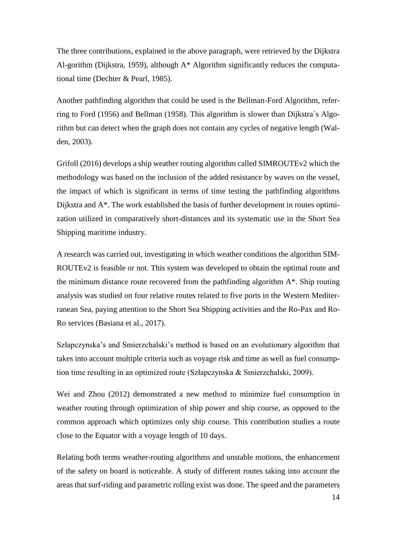
Grifoll (2016) develops a ship weather routing algorithm called SIMROUTEv2 which the
methodology was based on the inclusion of the added resistance by waves on the vessel,
the impact of which is significant in terms of time testing the pathfinding algorithms
Dijkstra and A*. The work established the basis of further development in routes optimi-
zation utilized in comparatively short-distances and its systematic use in the Short Sea
Shipping maritime industry.
A research was carried out, investigating in which weather conditions the algorithm SIM-
ROUTEv2 is feasible or not. This system was developed to obtain the optimal route and
the minimum distance route recovered from the pathfinding algorithm A*. Ship routing
analysis was studied on four relative routes related to five ports in the Western Mediter-
ranean Sea, paying attention to the Short Sea Shipping activities and the Ro-Pax and Ro-
Ro services (Basiana et al., 2017).
Szłapczynska’s and Smierzchalski’s method is based on an evolutionary algorithm that
takes into account multiple criteria such as voyage risk and time as well as fuel consump-
tion time resulting in an optimized route (Szłapczynska & Smierzchalski, 2009).
Wei and Zhou (2012) demonstrated a new method to minimize fuel consumption in
weather routing through optimization of ship power and ship course, as opposed to the
common approach which optimizes only ship course. This contribution studies a route
close to the Equator with a voyage length of 10 days.
Relating both terms weather-routing algorithms and unstable motions, the enhancement
of the safety on board is noticeable. A study of different routes taking into account the
areas that surf-riding and parametric rolling exist was done. The speed and the parameters

15
of the vessel were constant; the only alteration was the course of the vessel which was
avoiding the areas of these unstable motions. Indeed, real vessels have a limited maneu-
verability, and a tight zig-zag motion might be not always possible. Thus, they do not
believe in an increased grid resolution (Mannarini et al., 2013).
16
Aims and Objectives
Main objective
This project will introduce a new module based on ship unstable motions to the ship-
weather routing algorithm SIMROUTEv2. Unstable motions are evaluated through the
parameters such as peak wave period, emitted by the weather forecast, encountered pe-
riod, calculated by formula, and natural rolling period, established in the information of
each ship. With this new module, the algorithm will improve navigation in terms of safety,
consumption and contamination.
Specific objectives
Research the existent different types of motions of a ship (stable and unstable) and
identify the most frequent unstable motions to be considered for the case of study
Research and select the parameters of the ships which will be considered in this
study. The selection will be based on three different routes in the West Mediter-
ranean Sea
Research particular parameters of the waves related on the case of study
Implement the algorithm code in terms of unstable motions of the chosen ships
Run the simulations applied on the different cases and interpret the results
17
Methodology
In order to conduct the implementation of the ship-routing algorithm to avoid the frequent
unstable motions the following steps have been done:
On the one hand, an in-depth research of the different motions of the ship has been done
as the unstable motions are a consequence of the following 6 degrees of freedom of a
ship’s motions:
Translational motions: Heave, Sway and Surge
Rotational motions: Yaw, Pitch and Roll
On the other hand, a deep literature review was undertaken in order to know the common
variety of unstable motions to concern that is an important topic to take into account due
to the risk of suffering different damages (crew/passengers, cargo and ship). The unstable
motions found were:
Surf-riding/Broaching
Parametric rolling
Synchronous rolling
Slamming
Green water
Once the unstable motions research was done, it was considered to look into different
articles such as Mannarini et al., (2013) and Hansen & Pedersen (2008), among others,
and also focusing on the IMO Circulars (MSC.1/Circ.1228) in order to choose the most
frequent unstable motions to implement into SIMROUTEv2 algorithm. Finally, the work
was based on the two unstable motions that were possible to obtain the parameters related
on the formulas, surf-riding/broaching and parametric rolling. Other unstable motions
such as slamming, pressures upon the hull of the ship, among other parameters, were
required being the objective for possible future research.
A study of the formulation and the identification of the parameters required of make the
unstable motions (surf-riding/broaching and parametric rolling) was carried out.

18
Three hypothetical vessels were selected in this case of study. According to (Basiana et
al., 2017) vessels that carry vehicles and passengers with different speeds were selected,
due to the importance of these vessels in the Western Mediterranean Sea doing Short Sea
Shipping. These vessels and their particulars were the following:
Conventional ship (developing up to 23 knots)
Speed of the ship: 21.5 knots
Length of the ship: 166.41 meters
Beam of the ship: 25.5 meters
Draft of the ship: 14.29 meters
Transversal metacentric height: 2.63 meters
Fast ship (23 to 30 knots)
Speed of the ship: 28 knots
Length of the ship: 175.4 meters
Beam of the ship: 30.41 meters
Draft of the ship: 15.95 meters
Transversal metacentric height: 1.5 meters
High speed craft (more than 30 knots)
Speed of the ship: 40 knots
Length of the ship: 86.9 meters
Beam of the ship: 16.7 meters
Draft of the ship: 3.53 meters
Transversal metacentric height: 1.54 meters
The selected area for this study was Western Mediterranean Sea. The data was provided
from the contribution of (Basiana et al., 2017), who studied different ports considering
for their importance of Short Sea Shipping handling of goods. This work was conducted
on the following ports:
Port of Barcelona
Port of Oran
Port of Civitavecchia

19
Port of Sousse
Wave scripts were searched and obtained from the website Puertos del Estado (2016)
giving insight into daily weather patterns. Two different wave height scenarios were cho-
sen for each route:
Smooth-Moderate sea; Hs = 0.1-2.50 meters
Rough-High sea; Hs = 2.5-9.00 meters
In the aforementioned wave scripts, two weather parameters were taken into account in
order to see if surf-riding/broaching and parametric rolling occurred:
Wave direction
Wave period
Different cases of study were run in order to find cases of surf-riding/broaching and par-
ametric rolling in the different routes.
SIMROUTEv2 was the ship-weather routing algorithm used for this project. A summary
of the algorithm and its structural basis (route function and wave function) was provided.
Additionally, a description of how the algorithm works (the use of important commands
that are taken into account) was given.
The results of the specific cases were provided by the algorithm. In each case, the route
can be seen in blue color and the length of the nodes that had unstable motions in red. All
the cases were calculated by SIMROUTEv2.
Finally, some conclusions from the results were done. Specific cases where these two
unstable motions occurred were highlighted.
20
1. General motions of a ship
1.1. Stable motions
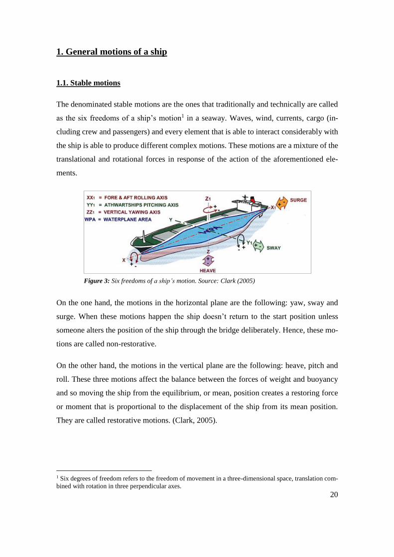
The denominated stable motions are the ones that traditionally and technically are called
as the six freedoms of a ship’s motion1 in a seaway. Waves, wind, currents, cargo (in-
cluding crew and passengers) and every element that is able to interact considerably with
the ship is able to produce different complex motions. These motions are a mixture of the
translational and rotational forces in response of the action of the aforementioned ele-
ments.
On the one hand, the motions in the horizontal plane are the following: yaw, sway and
surge. When these motions happen the ship doesn’t return to the start position unless
someone alters the position of the ship through the bridge deliberately. Hence, these mo-
tions are called non-restorative.
On the other hand, the motions in the vertical plane are the following: heave, pitch and
roll. These three motions affect the balance between the forces of weight and buoyancy
and so moving the ship from the equilibrium, or mean, position creates a restoring force
or moment that is proportional to the displacement of the ship from its mean position.
They are called restorative motions. (Clark, 2005).
1 Six degrees of freedom refers to the freedom of movement in a three-dimensional space, translation com-
bined with rotation in three perpendicular axes.
Figure 3: Six freedoms of a ship’s motion. Source: Clark (2005)
21
Table 1: Classification of the six degrees of freedom. Source: Own elaboration
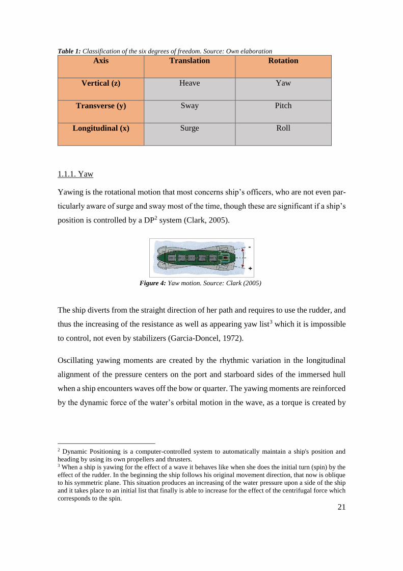
1.1.1. Yaw
Yawing is the rotational motion that most concerns ship’s officers, who are not even par-
ticularly aware of surge and sway most of the time, though these are significant if a ship’s
position is controlled by a DP2 system (Clark, 2005).
The ship diverts from the straight direction of her path and requires to use the rudder, and
thus the increasing of the resistance as well as appearing yaw list3 which it is impossible
to control, not even by stabilizers (Garcia-Doncel, 1972).
Oscillating yawing moments are created by the rhythmic variation in the longitudinal
alignment of the pressure centers on the port and starboard sides of the immersed hull
when a ship encounters waves off the bow or quarter. The yawing moments are reinforced
by the dynamic force of the water’s orbital motion in the wave, as a torque is created by
2 Dynamic Positioning is a computer-controlled system to automatically maintain a ship's position and
heading by using its own propellers and thrusters. 3 When a ship is yawing for the effect of a wave it behaves like when she does the initial turn (spin) by the
effect of the rudder. In the beginning the ship follows his original movement direction, that now is oblique
to his symmetric plane. This situation produces an increasing of the water pressure upon a side of the ship
and it takes place to an initial list that finally is able to increase for the effect of the centrifugal force which
corresponds to the spin.
Axis Translation Rotation
Vertical (z) Heave Yaw
Transverse (y) Sway Pitch
Longitudinal (x) Surge Roll
Figure 4: Yaw motion. Source: Clark (2005)

22
the water at a wave crest pushing the hull direction of the wave whilst the water in a
trough is pushing in the opposite direction4 (Clark, 2005).
1.1.2. Sway
Waves, winds and currents are the three most relevant factors that produce the transla-
tional motion called sway. In general, the higher the relation between the emerged hull
and the immersed hull of the ship the most sway is able to suffer.
Looking into a wave cycle and taking into account that a ship is stationary and there is a
beam sea wave celerity coming from starboard to port side the following process happens:
1. Ship situated on the crest of the wave: sway velocity is maximum to port through
mean position
2. The ship is descending: Sway velocity is zero, port displacement is maximum
3. Ship situated on the trough of the wave: Sway velocity is maximum to starboard
through mean position
4. Sway velocity is zero, starboard displacement is maximum
5. End of the process: Sway velocity is maximum to port through mean position
4 The orbital motion in deep waters follows a circumference shape in rotational movement where the crest
moves on the same sense of the wave, while the under part of the surface moves on the other sense. In
contrast, when the coast is nearer, in shallow waters, the shape evolves into an ellipse.
Figure 5: Sway motion. Source: Clark (2005)
Figure 6: Wave cycle and ship positions. Source: Own elaboration

23
1.1.3. Surge
When the water flow is passing a ship creates a resistance that acts on the immersed hull
surface to accelerate the vessel in the same direction of the flow at a rate that is propor-
tional to the ship´s virtual mass5. The added mass for the translational motion called surge
is only about 6-10% of normally shaped ship, which to be expected as the ship-shaped
hull is built to move fore and aft having the least resistance from the water (Clark, 2005).
Although this translational movement in the longitudinal axis is governed by the main
propeller going back or forward, it is known that the external forces (waves, winds and
currents) acts indirectly to the ship influencing surge motion in a positive or negative way.
1.1.4. Heave
This is the vertical translational upward or downward movement in the water of the ship’s
center of gravity. This restorative motion is compared as a mass-damper-spring system,
such as a suspension of a car.
When a ship is submerging more than the equilibrium waterline, there is an excess of
buoyancy6. An excessive downward heave can swamp the ship (Clark, 2005).
5 Ship’s mass plus added water mass. 6 Where ‘Z’ is the downward or upward displacement from the equilibrium waterline; ‘𝜌’ is the water
density (kg/m3); ‘g’ is the gravity (m/s2) and WPA is the waterplane area of the hull (m2).
Figure 7: Surge motion. Source: Clark (2005)
Figure 8: Heave motion. Source: Clark (2005)
24
𝐸𝑥𝑐𝑒𝑠𝑠𝑏𝑢𝑜𝑦𝑎𝑛𝑐𝑦 = −𝑍𝜌𝑔(𝑊𝑃𝐴) (1)
Looking to the other way round, if the ship is emerging above the equilibrium waterline
there is an excess of weight (Clark, 2005).
𝐸𝑥𝑐𝑒𝑠𝑠𝑤𝑒𝑖𝑔ℎ𝑡 = +𝑍𝜌𝑔(𝑊𝑃𝐴) (2)
So the natural heave period7 is:
𝑇0 = 2𝜋√𝑀𝑣
𝜌𝑔(𝑊𝑃𝐴) (3)
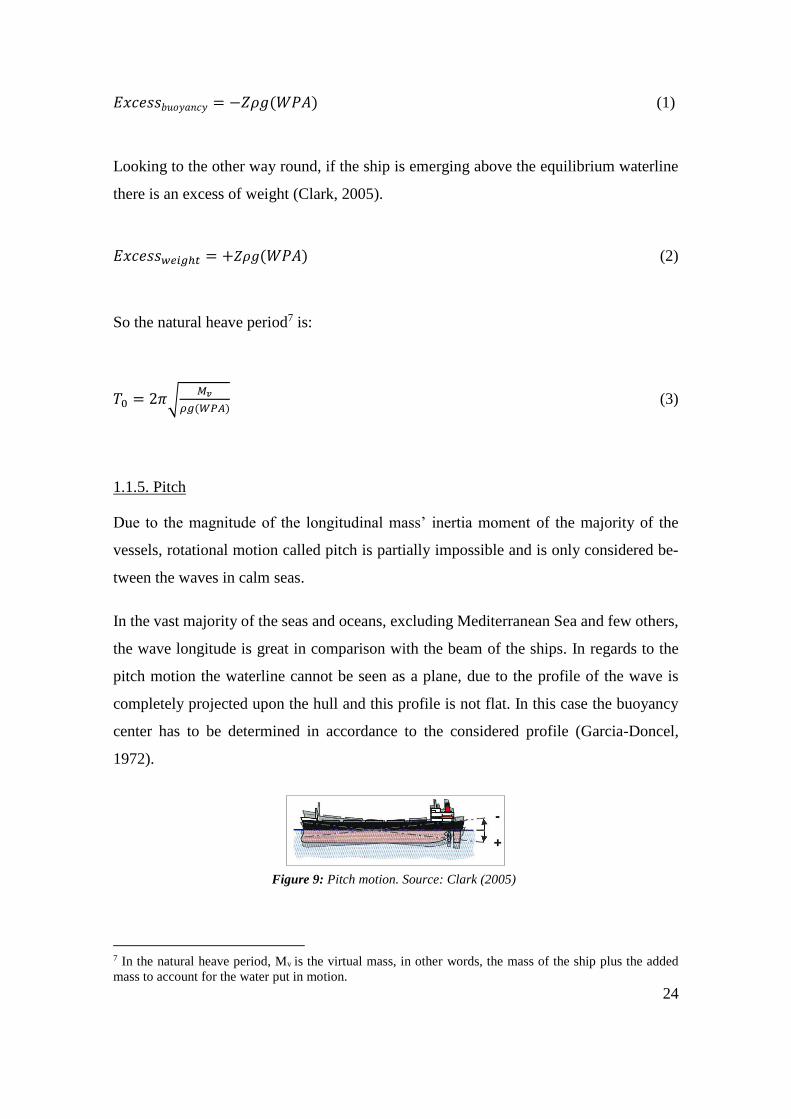
1.1.5. Pitch
Due to the magnitude of the longitudinal mass’ inertia moment of the majority of the
vessels, rotational motion called pitch is partially impossible and is only considered be-
tween the waves in calm seas.
In the vast majority of the seas and oceans, excluding Mediterranean Sea and few others,
the wave longitude is great in comparison with the beam of the ships. In regards to the
pitch motion the waterline cannot be seen as a plane, due to the profile of the wave is
completely projected upon the hull and this profile is not flat. In this case the buoyancy
center has to be determined in accordance to the considered profile (Garcia-Doncel,
1972).
7 In the natural heave period, Mv is the virtual mass, in other words, the mass of the ship plus the added
mass to account for the water put in motion.
Figure 9: Pitch motion. Source: Clark (2005)

25
Encountered wavelengths much longer than the ship generally also have long periods of
encounter so the ship follows the fore and aft wave profile without any significant phase
lag. The vessel rides the waves easily and though the trim angle varies with the horizontal,
it remains nearly parallel to the waterline so the pitching moments are minimum. In other
words, if the wave period is significantly longer than the ship’s pitching period its trim
will tend to follow quite close behind the wave profile and the ship should climb and
descend each wave in a normal way. The ship’s natural pitching period8 is the following
one:
𝑇𝑃 = 2√𝑘 × 𝑑 (4)
1.1.6. Roll
This rotational motion in which the ‘springiness’9 is due to wave action moving the forces
of weight and buoyancy out of vertical alignment as buoyancy distribution changes with
the alternating waterline slope across the ship’s beam. This situation creates a righting
moment to reestablish the ship to the stable or optimal position that is approximately
proportional to the ship’s inclined angle to the waterline when the angle is small. If the
vessel suffers an external force repeatedly, it will balance with inclination angle that will
be different according to the value and the rhythm of the applied force.
From the moment when the external force is not zero, the moment of righting acts and
produces the turn of the ship to the upright position, so that the total energy stored in the
8 ‘k’ is the correction factor for the moment of inertia of the added mass; ‘d’ means the draft of the vessel. 9 Understanding springiness as the capacity of straighten the vessel with respect to its vertical axes.
Figure 10: Roll motion. Source: Clark (2005)

26
inclined position acts as kinetic energy that takes the ship to a symmetrical position with
the previous one in relation to the longitudinal resting plane, repeating this movement
indefinitely. (Garcia-Doncel, 1972).
The natural roll period, in terms of ‘GM’ and radius of gyration10 is the following one:
𝑇 = 2𝜋√𝑅𝑣
2
𝐺𝑀 × 𝑔 (5)
1.2. Unstable motions
Operational conditions depend, in large part, on the stations of the year and the navigation
area, as well as other conditions. Despite its importance, it is an aspect that has been little
studied when it comes to making the project of the ship. The idea of ship’s comfortability
has just begun to develop recently, thanks in part to the new applications.
When a ship navigates with sufficiently large waves in relation to its size, it experiences
undesirable movements that can cause discomfort to the passage, crew members, gener-
ation of dynamic loads to the structure and cargo of the ship. These undesirable move-
ments are the so-called unstable motions produced by these external meteorological phe-
nomena and are combinations of the six degrees of freedom of the ship. There are several
types of unstable motions and they depend at least on the speed, displacement, weight
distribution, hull design and location of the appendages.
1.2.1. Surf riding/Broaching
One of these unstable motions is surf-riding and consequent broaching which are associ-
ated with following and quartering seas. Large following waves acting on the ship can
force her to move with the same speed, so a ride upon the wave happens and is able to
provoke a rough twist and a considerable heel to the vessel and can finish with a capsize.
10 Rv could be expressed as 0.4 x Beam.

27
The phenomenon which the vessel starts to move with the wave simultaneously is known
as surf-riding. The vast majority of the vessels are directionally unstable during waves.
As can be seen in Figure 11, the vessel is in following seas and presents a clear unstable
motion of surf-riding. It is starting to ride on the crest and once the wave has passed the
length of the vessel, it starts to do a considerable heel that could conclude to a broaching
motion.
The moment that the vessel is turning in an uncontrolled way is called broaching. Broach-
ing endangers the ship to capsize as a result of the circumstance of an unexpected change
of the ship’s heading and an important heel angle produced by circulation and wave heel-
ing moment usually acting in the same direction.
Figure 11: Simulation of surf-riding. Source: Umeda
(2015)

28
When a ship is riding on the wave crest, the intact stability can be reduced considerably
according to the alteration of the submerged hull form. This stability reduction may be-
come critical for wave lengths between the range of 0.6 L11 up to 2.3 L. When the wave
length is found within these values the amount of stability reduction is nearly proportional
to the wave height. This situation is extremely dangerous in following and quartering
seas, due to the increase of the duration of riding on the wave crest, which coincides to
the time interval of reduced stability (IMO, MSC.1/Circ.1228, 2007).
Officers of a ship are recommended to take care of the following instructions in order to
avoid the dangerous situations when navigating in severe weather conditions:
It has to be taken into account that surf-riding and broaching-to may occur when
both of these conditions12 are fulfilled (Mannarini et al., 2013):
135° < 𝛼 < 225° (6)
And also:
11 ‘L’ is the ship’s length in meters. 12 Being ′𝛼′ the ship-to-wave relative direction in degrees , ‘′𝐿𝑠ℎ𝑖𝑝′ the length of the ship in meters and 𝑣𝑠ℎ𝑖𝑝
the speed of the ship in knots.
Figure 12: The risk of broaching in heavy following seas. Source: Clark (2005)
29
𝑣𝑠ℎ𝑖𝑝 >1.8√𝐿𝑠ℎ𝑖𝑝
cos (180°−𝛼) (7)
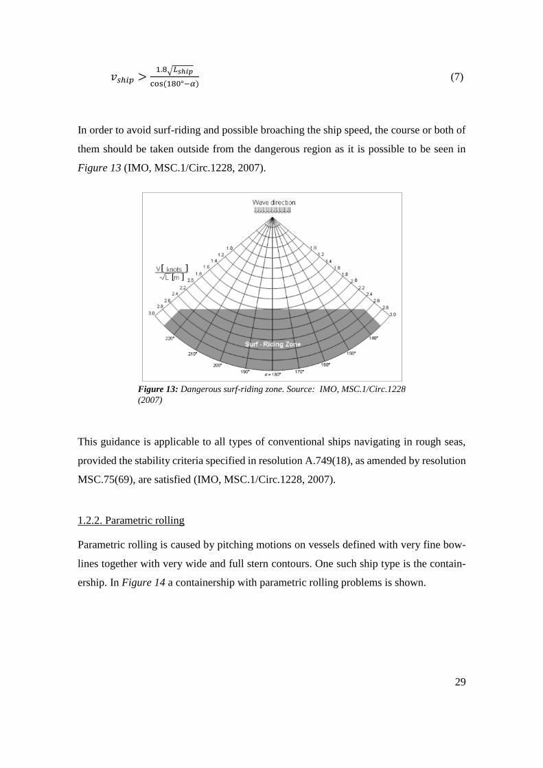
In order to avoid surf-riding and possible broaching the ship speed, the course or both of
them should be taken outside from the dangerous region as it is possible to be seen in
Figure 13 (IMO, MSC.1/Circ.1228, 2007).
This guidance is applicable to all types of conventional ships navigating in rough seas,
provided the stability criteria specified in resolution A.749(18), as amended by resolution
MSC.75(69), are satisfied (IMO, MSC.1/Circ.1228, 2007).
1.2.2. Parametric rolling
Parametric rolling is caused by pitching motions on vessels defined with very fine bow-
lines together with very wide and full stern contours. One such ship type is the contain-
ership. In Figure 14 a containership with parametric rolling problems is shown.
Figure 13: Dangerous surf-riding zone. Source: IMO, MSC.1/Circ.1228
(2007)

30
The cause of this phenomenon depends very much on the parameters of the vessel, hence
the name parametric rolling.
On the one hand, when TE = TR (encounter ratio 1:1) the stability attains a minimum once
during each roll period. This situation is characterized by asymmetric rolling, for instance
the amplitude with the wave crest amidships is bigger than the amplitude to the other side.
Due to the large amplitude a retarded up-right is produced and the roll period TR may
adapt to the encounter period to a certain extent, so that this kind of parametric rolling
may occur with a wide bandwidth of encounter periods. In quartering seas, a transition to
harmonic resonance may become appreciable (IMO, MSC.1/Circ.1228, 2007).
On the other hand, when TE = 1/TR (encounter ratio 1:0.5). The stability attains a mini-
mum twice during each roll period. In the situations of following or quartering seas, where
the encounter period is larger than the wave period, this may only occur with very large
roll periods TR, indicating a marginal intact stability. As a consequence, symmetric rolling
happens with large amplitudes, again with the tendency of adapting the ship response to
the period of encounter because of the loss of stability when the ship is on the wave crest.
Parametric rolling with encounter ratio 1:0.5 may also occur in head and bow seas (IMO,
MSC.1/Circ.1228, 2007).
Figure 14: Parametric rolling of a fine lined hull with a full stern. Source: Clark (2005)

31
Apart from following and quartering seas, where the change of stability is only affected
by the waves that pass along the ship, heavy heave and pitch motions that are frequent in
head or bow seas may contribute to enlarge the variation of the stability, specifically due
to the periodical immersion and emersion of the flared stern frames and flared bows of
modern ships. This may conduct to dangerous parametric roll motions even with stability
variations induced by small waves (IMO, MSC.1/Circ.1228, 2007).
As the stern dips into the waves it produces a rolling action. This remains unchecked as
the bow next dips into the waves due to pitching forces. It is worst when TE = TR or when
TE = 1/TR.
In effect, the rolling characteristics are quite different at the bow to the ones at the stern.
This situation produces a twisting or torsioning along the ship as can be seen in Figure
15, leading to extra rolling motions.
Parametric rolling will only happen if a steady angle of heel or list exists, such as may be
created by the cargo inequalities in different parts of the vessel, the wind acting on one of
the emerged sides or the fuel between the starboard and port sides. Normally, the officers
of the ship try to ensure that cargo is properly loaded and fuel is drawn equally from tanks
that are usually daily alternated between the starboard and port sides of the ship but, even
though, a little list can appear, and obviously, wind heel is hardly ever avoidable.
Figure 15: Parametric rolling on a container vessel.
Source: Barrass & Derrett (2012)

32
It has to be taken into account that parametric rolling may occur when one of these fol-
lowing conditions13 are fulfilled (Mannarini et al., 2013):
|𝑇𝐸 − 𝑇𝑅| = 𝜀 × 𝑇𝑅 (8)
Or:
|2𝑇𝐸 − 𝑇𝑅| = 𝜀 × 𝑇𝑅 (9)
When a ship is operating at reduced speed in heavy sea conditions the phenomenon of
parametric rolling is even worse. In this condition containers are able to be lost overboard
because of the broken deck lashings. Parametric rolling problems are least on box-shaped
vessels or full-form barges where the forward and aft shapes are not too different (Barrass
& Derrett, 2012).
In order to avoid parametric rolling in quartering, following, head, bow or beam seas it is
necessary to select the course and the speed of the vessel in a way to stay away from the
aforementioned conditions: the encounter period is close to one half of the ship roll period
(TE = approximately equal 0.5×TR) or the encounter period is close to the ship roll period
(TE = approximately equal TR).
13 Being ‘𝜀’ the tolerance, ‘TE’ the encountered period and ‘TR’ the natural roll period.
33
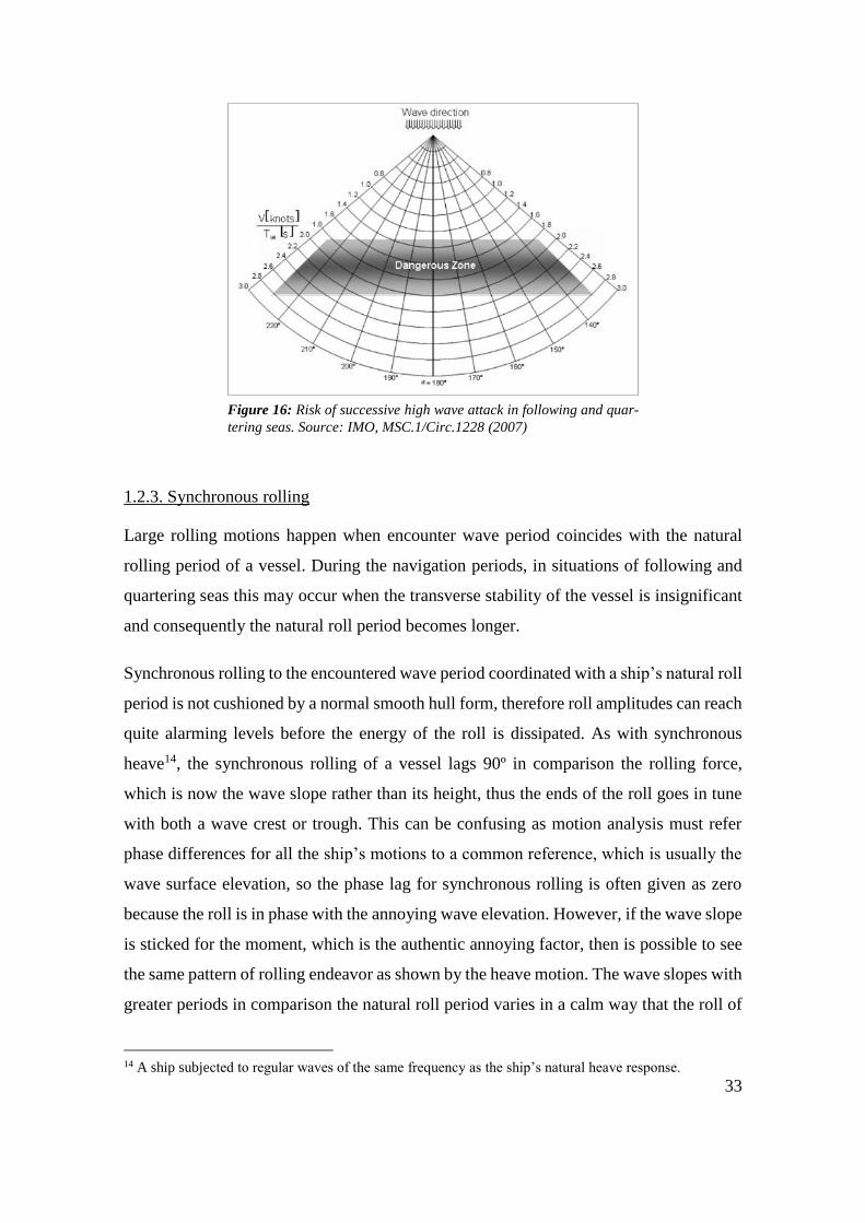
1.2.3. Synchronous rolling
Large rolling motions happen when encounter wave period coincides with the natural
rolling period of a vessel. During the navigation periods, in situations of following and
quartering seas this may occur when the transverse stability of the vessel is insignificant
and consequently the natural roll period becomes longer.
Synchronous rolling to the encountered wave period coordinated with a ship’s natural roll
period is not cushioned by a normal smooth hull form, therefore roll amplitudes can reach
quite alarming levels before the energy of the roll is dissipated. As with synchronous
heave14, the synchronous rolling of a vessel lags 90º in comparison the rolling force,
which is now the wave slope rather than its height, thus the ends of the roll goes in tune
with both a wave crest or trough. This can be confusing as motion analysis must refer
phase differences for all the ship’s motions to a common reference, which is usually the
wave surface elevation, so the phase lag for synchronous rolling is often given as zero
because the roll is in phase with the annoying wave elevation. However, if the wave slope
is sticked for the moment, which is the authentic annoying factor, then is possible to see
the same pattern of rolling endeavor as shown by the heave motion. The wave slopes with
greater periods in comparison the natural roll period varies in a calm way that the roll of
14 A ship subjected to regular waves of the same frequency as the ship’s natural heave response.
Figure 16: Risk of successive high wave attack in following and quar-
tering seas. Source: IMO, MSC.1/Circ.1228 (2007)
34
the vessel can balance with the profile of the wave and keep in phase with the wave slope.
In the situation of shorter period, wave slopes varies so quickly that the lags of the roll
are approximately 180º behind as the roll response of the ship to each wave is stopped by
the arrival of the following wave (Clark, 2005).
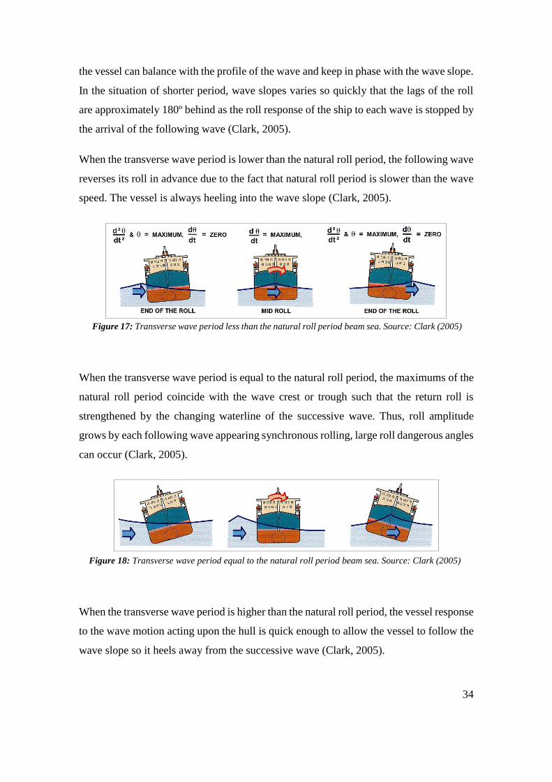
When the transverse wave period is lower than the natural roll period, the following wave
reverses its roll in advance due to the fact that natural roll period is slower than the wave
speed. The vessel is always heeling into the wave slope (Clark, 2005).
When the transverse wave period is equal to the natural roll period, the maximums of the
natural roll period coincide with the wave crest or trough such that the return roll is
strengthened by the changing waterline of the successive wave. Thus, roll amplitude
grows by each following wave appearing synchronous rolling, large roll dangerous angles
can occur (Clark, 2005).
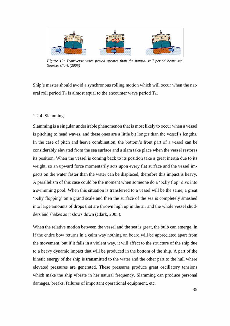
When the transverse wave period is higher than the natural roll period, the vessel response
to the wave motion acting upon the hull is quick enough to allow the vessel to follow the
wave slope so it heels away from the successive wave (Clark, 2005).
Figure 17: Transverse wave period less than the natural roll period beam sea. Source: Clark (2005)
Figure 18: Transverse wave period equal to the natural roll period beam sea. Source: Clark (2005)
35
Ship’s master should avoid a synchronous rolling motion which will occur when the nat-
ural roll period TR is almost equal to the encounter wave period TE.
1.2.4. Slamming
Slamming is a singular undesirable phenomenon that is most likely to occur when a vessel
is pitching to head waves, and these ones are a little bit longer than the vessel’s lengths.
In the case of pitch and heave combination, the bottom’s front part of a vessel can be
considerably elevated from the sea surface and a slam take place when the vessel restores
its position. When the vessel is coming back to its position take a great inertia due to its
weight, so an upward force momentarily acts upon every flat surface and the vessel im-
pacts on the water faster than the water can be displaced, therefore this impact is heavy.
A parallelism of this case could be the moment when someone do a ‘belly flop’ dive into
a swimming pool. When this situation is transferred to a vessel will be the same, a great
‘belly flopping’ on a grand scale and then the surface of the sea is completely smashed
into large amounts of drops that are thrown high up in the air and the whole vessel shud-
ders and shakes as it slows down (Clark, 2005).
When the relative motion between the vessel and the sea is great, the bulb can emerge. In
If the entire bow returns in a calm way nothing on board will be appreciated apart from
the movement, but if it falls in a violent way, it will affect to the structure of the ship due
to a heavy dynamic impact that will be produced in the bottom of the ship. A part of the
kinetic energy of the ship is transmitted to the water and the other part to the hull where
elevated pressures are generated. These pressures produce great oscillatory tensions
which make the ship vibrate in her natural frequency. Slamming can produce personal
damages, breaks, failures of important operational equipment, etc.
Figure 19: Transverse wave period greater than the natural roll period beam sea.
Source: Clark (2005)
36
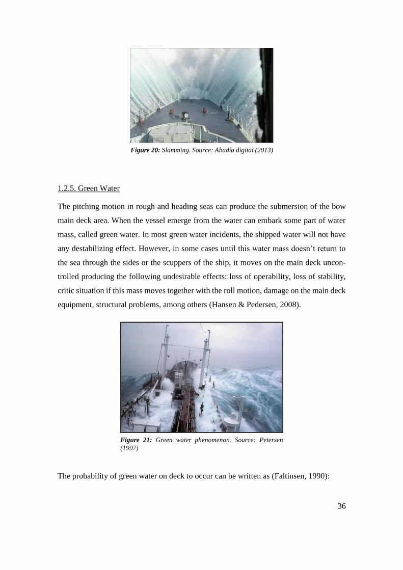
1.2.5. Green Water
The pitching motion in rough and heading seas can produce the submersion of the bow
main deck area. When the vessel emerge from the water can embark some part of water
mass, called green water. In most green water incidents, the shipped water will not have
any destabilizing effect. However, in some cases until this water mass doesn’t return to
the sea through the sides or the scuppers of the ship, it moves on the main deck uncon-
trolled producing the following undesirable effects: loss of operability, loss of stability,
critic situation if this mass moves together with the roll motion, damage on the main deck
equipment, structural problems, among others (Hansen & Pedersen, 2008).
The probability of green water on deck to occur can be written as (Faltinsen, 1990):
Figure 20: Slamming. Source: Abadía digital (2013)
Figure 21: Green water phenomenon. Source: Petersen
(1997)
37
𝑃(𝐺𝑟𝑒𝑒𝑛𝑊𝑎𝑡𝑒𝑟) = 𝑒𝑥𝑝 [−𝑑𝑓
2
2𝜎𝑟2] (10)
Where 𝑑𝑓 is the freeboard distance and 𝜎𝑟2 is the variance of the relative motion.
38
2. Unstable motions parameters
The IMO MSC.1/Circ.1228 concerns the officers with the different formulas of the two
unstable motions worked in the case of study. The parameters and the constants which
compose these formulas are the key to safe the vessel, its cargo, passengers and crew
members. Managing these parameters will be a good method for avoiding vessels getting
into the dangerous areas aforementioned in the section 1.2.1 and 1.2.2.
Fixed parameters are obtained from three hypothetical different vessels. The first vessel
is a Conventional Ship, developing a speed of 21.5 knots. The second vessel is a Fast Ship
which has a speed of 28 knots. The third vessel is a High Speed Craft (HSC) with a speed
of 40 knots. These vessels were chosen in order to see if unstable motions can occur to
vessels with different speeds. It has to be taken into account that a HSC would not do
these large routes.
Considering the distribution by sea regions, Mediterranean ports handled the most tonnage at
29% of the total EU Short Sea Shipping tonnages in 2015. In addition, two of the vessels
chosen are inspired in Ro-Pax vessels which represents the 13% of the vessels handling goods
in the Mediterranean Sea in 2015. Although this is not a very large representative amount in
contrast with the other type of cargo, it has been chosen for the study of this paper due to the
benefits that these vessels contribute. This contribution can be seen in terms of environmental
protection, transport safety and decongestion of roads, that is, the less trucks in the roads, the
fewer pollutants in the atmosphere, the fewer traffic accidents and the traffic would be more
fluid. For these reasons this area and these three vessels have been selected in this case of
study (Basiana et al., 2017).
Moreover, the selection of the unstable motions was based on the different parameters that
were available. Hence, surf-riding/broaching and parametric rolling were the two unstable
motions selected for being implemented into the algorithm due to the fact that parameters of
their formulas were obtained through the three aforementioned vessels and because the
IMO MSC.1/Circ.1228 give relevance to both of them.
39
2.1. Surf-riding/Broaching parameters
As it is seen in the formulas of surf-riding/broaching phenomenon
135° < 𝛼 < 225° (6)
And also:
𝑣𝑠ℎ𝑖𝑝 >1.8√𝐿𝑠ℎ𝑖𝑝
cos (180°−𝛼) (7)
In regards of this formula, the parameters are the following ones:
- Angle of encounter (𝜶)
Angle 𝛼 being the ship-to-wave relative direction (𝛼 = 180° for following seas).
In other words, the wave direction angle minus the vessel course.
- Length of the ship (Lship)
In this case of study, the distance between the distance between the perpendicu-
lars.
- Speed of the ship (vship)
The speed selected for this study is the one which corresponds to the full sea ahead
engine order.

40
2.2. Parametric rolling parameters
As said before, so that parametric rolling phenomenon occurs one of these following for-
mulas have to be true:
|𝑇𝐸 − 𝑇𝑅| = 𝜀 × 𝑇𝑅 (8)
Or:
|2𝑇𝐸 − 𝑇𝑅| = 𝜀 × 𝑇𝑅 (9)
In regards of this formula, the parameters are the following ones:
- Tolerance in period matching (𝜺)
The value that has been chosen for this parameter is a 10% and it is obtained from
the article of Mannarini et al. (2013).
- Encountered period (TE)
The period of encounter TE could be either measured as the period of pitching by
using stop watch or calculated by the Formula (11), where ‘v’ is ship’s speed in
Table 2: Example of the speeds depending on engine order from the PASSENGER FERRY 8.
Source: TRANSAS (2014)

41
knots and ‘α’ the angle between keel direction and wave direction (α = 0° means
head sea).
(11)
The diagram in Figure 22 may as well be used for the determination of encounter
period.
- Natural roll period (TR)
It measures the period of rolling motions preferably when the ship is in calm sea.
This period is obtained through the following formulas, and the parameters are
taken from the vessel chosen (model from a simulator).
(12)
Figure 22: Determination of the period of encounter TE. Source: IMO,
MSC.1/Circ.1228 (2007)
42
- Coefficient (C)
(13)
- Beam of the ship (B)
The overall width of the ship measured at the widest point of the nominal water-
line.
- Draft of the ship (d)
The vertical distance from the bottom of the keel to the waterline.
- Metacentric height of the ship (GM)
The measurement of the initial static stability of a floating body.
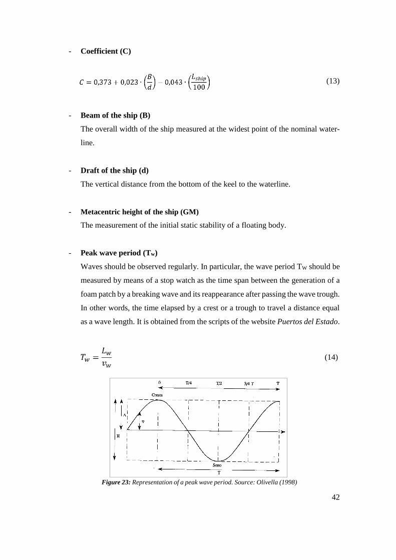
- Peak wave period (Tw)
Waves should be observed regularly. In particular, the wave period TW should be
measured by means of a stop watch as the time span between the generation of a
foam patch by a breaking wave and its reappearance after passing the wave trough.
In other words, the time elapsed by a crest or a trough to travel a distance equal
as a wave length. It is obtained from the scripts of the website Puertos del Estado.
(14)
Figure 23: Representation of a peak wave period. Source: Olivella (1998)

43
- Wave length (Lw)
The wave length is determined either by visual observation in comparison with
the ship length or by reading the mean distance between successive wave crests
on the radar images of waves.
- Wave speed (vw)
This parameter depends of the wave length and the period of the wave. Waves of
different periods and lengths will be propagated with different speeds, being so
dispersive. A fact that is based on observation is that the large waves travel faster
than the short waves.
If the definitions of frequency {𝑤 =2𝜋
𝐿𝑤} and number of wave {𝑘 =
2𝜋
𝑇𝑤} are
taken into account, the wave speed will depend on these parameters:
(15)
44
3. SIMROUTEv2
3.1. Basis and Algorithm
The two well-known pathfinding algorithms normally used are the Dijkstra Algorithm
(Dijkstra, 1959) and the A* Algorithm (Dechter and Pearl, 1985). Dijkstra Algorithm was
tested in some investigations and it is configured in the SIMROUTEv2. However, it was
proved, in terms of calculation time, that A* Algorithm was much faster. For this reason,
A* Algorithm was selected to do this case of study.
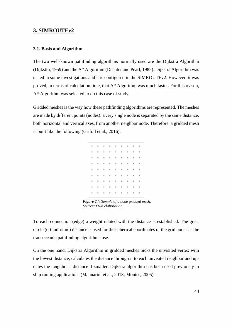
Gridded meshes is the way how these pathfinding algorithms are represented. The meshes
are made by different points (nodes). Every single node is separated by the same distance,
both horizontal and vertical axes, from another neighbor node. Therefore, a gridded mesh
is built like the following (Grifoll et al., 2016):
To each connection (edge) a weight related with the distance is established. The great
circle (orthodromic) distance is used for the spherical coordinates of the grid nodes as the
transoceanic pathfinding algorithms use.
On the one hand, Dijkstra Algorithm in gridded meshes picks the unvisited vertex with
the lowest distance, calculates the distance through it to each unvisited neighbor and up-
dates the neighbor’s distance if smaller. Dijkstra algorithm has been used previously in
ship routing applications (Mannarini et al., 2013; Montes, 2005).
Figure 24: Sample of a node gridded mesh.
Source: Own elaboration

45
On the other hand, A* algorithm finds solutions by looking at all the possible path com-
binations to the result (goal) for the one that obtains the minimum cost (shortest time,
shortest distance travelled, etc..) and among these paths it selects the ones that appear to
be the fastest to the solution. It is depicted in terms of weighted graphs: beginning from
a particular node of a graph, it creates a tree of paths, expanding all these paths one node
at a time, until one of the paths reach a predestined goal node. At each repetition of its
main loop, A* algorithm needs to establish which of its unfinished paths to expand into
one or more longer paths (Grifoll et al., 2016).
𝑓(𝑛) = 𝑔(𝑛) + ℎ(𝑛) (16)
Where “n” is the last node on the path, g(n) is the cost of the path from the start node to
“n”, and h(n) is a heuristic that estimates the cost of the cheapest path from n to the goal.
The heuristic is problem-specific. For the algorithm to find the actual shortest path, the
heuristic function must be admissible, meaning that it never overestimates the actual cost
to get the nearest goal node. In the case of the study, the heuristic function is the minimum
distance between origin and destination (Grifoll et al., 2016).
In function of the grid resolution, path connection options between nodes may vary. In
consequence, the sequence of edges followed by the shortest path will be limited by the
grid resolution and the connected nodes. As it is seen in Figure 25, edges are connecting
nodes displayed by arrows. Every single arrow represents different potential ship courses
or directions. Grid resolution can vary according to the investigator’s preferences. In this
work, different grid resolution has been tested obtaining similar conclusions than (Man-
narini et al., 2013), which contemplated that at least 16 edges are required in order to be
precise (Grifoll et al., 2016).

46
3.2. Waves
Ships can experience challenging operating conditions due to a constant action of waves.
Complete knowledge of the expected sea states is important when considering vessel
safety.
Wave action is the major factor that affects the ship performance and safety navigation
(Hu et al., 2014). Wave field affects the ship motions decreasing the propeller thrust and
adding a resistance in comparison to absence of waves. A simple formula to include ship
speed reduction to waves is suggested by (Bowditch, 2002). The final speed is computed
in function of the non-wave affected speed (v0) plus a reduction in function of the wave
parameters (Grifoll et al., 2016):
𝑣(𝐻, 𝛩) = 𝑣0 − 𝑓(𝛩) · 𝐻2 (17)
Where H is the significant wave height and f is a parameter in function of the relative ship
wave direction. The values of f coefficient are shown in Table 3 (Grifoll et al., 2016).
Figure 25: Scheme of the grid resolution, 16
edges per node. Source: Own elaboration
47
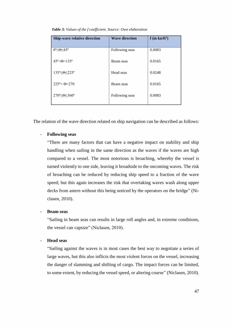
Table 3: Values of the f coefficient. Source: Own elaboration
Ship-wave relative direction Wave direction f (in kn/ft2)
0º≤Θ≤45º Following seas 0.0083
45º<Θ<135º Beam seas 0.0165
135º≤Θ≤225º Head seas 0.0248
225º< Θ<270 Beam seas 0.0165
270º≤Θ≤360º Following seas 0.0083
The relation of the wave direction related on ship navigation can be described as follows:
- Following seas
“There are many factors that can have a negative impact on stability and ship
handling when sailing in the same direction as the waves if the waves are high
compared to a vessel. The most notorious is broaching, whereby the vessel is
turned violently to one side, leaving it broadside to the oncoming waves. The risk
of broaching can be reduced by reducing ship speed to a fraction of the wave
speed; but this again increases the risk that overtaking waves wash along upper
decks from astern without this being noticed by the operators on the bridge” (Ni-
clasen, 2010).
- Beam seas
“Sailing in beam seas can results in large roll angles and, in extreme conditions,
the vessel can capsize” (Niclasen, 2010).
- Head seas
“Sailing against the waves is in most cases the best way to negotiate a series of
large waves, but this also inflicts the most violent forces on the vessel, increasing
the danger of slamming and shifting of cargo. The impact forces can be limited,
to some extent, by reducing the vessel speed, or altering course” (Niclasen, 2010).
48
- Quartering sea
“Large quartering waves are unfortunate because the vessel stability is affected
by the negative effects of both beam and following seas” (Niclasen, 2010).
- Crossing sea
“It is always difficult to handle small vessels in severe sea, but severe crossing
sea is particularly dangerous as the waves will approach a vessel from different
directions. In such circumstances, the captain loses the ability to use the vessel
heading to protect against beam seas” (Niclasen, 2010).
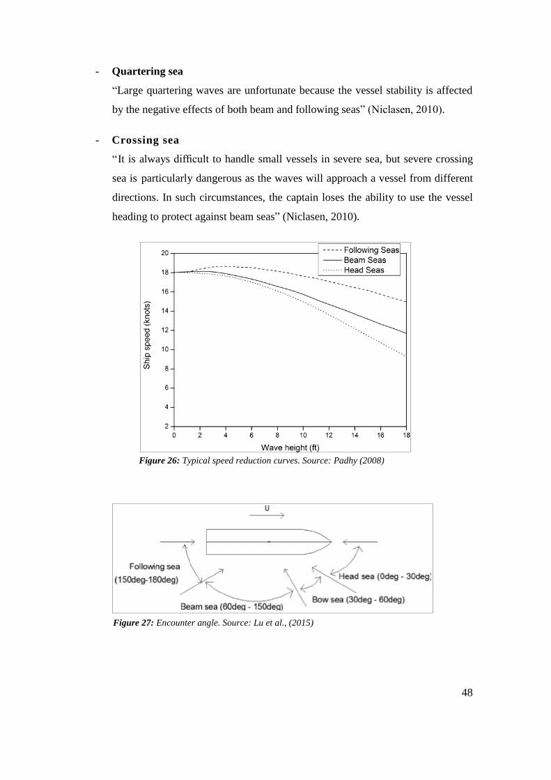
Figure 26: Typical speed reduction curves. Source: Padhy (2008)
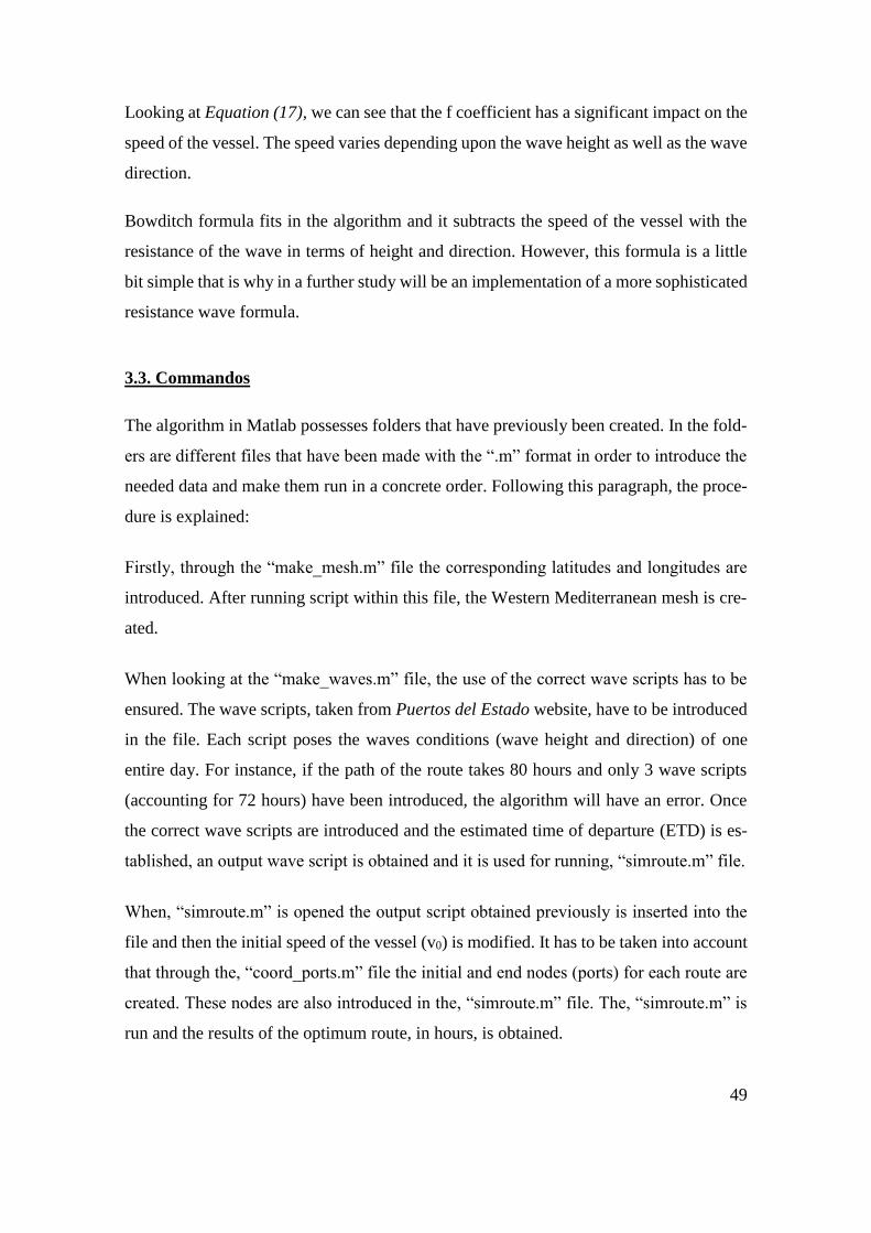
Figure 27: Encounter angle. Source: Lu et al., (2015)
49
Looking at Equation (17), we can see that the f coefficient has a significant impact on the
speed of the vessel. The speed varies depending upon the wave height as well as the wave
direction.
Bowditch formula fits in the algorithm and it subtracts the speed of the vessel with the
resistance of the wave in terms of height and direction. However, this formula is a little
bit simple that is why in a further study will be an implementation of a more sophisticated
resistance wave formula.
3.3. Commandos
The algorithm in Matlab possesses folders that have previously been created. In the fold-
ers are different files that have been made with the “.m” format in order to introduce the
needed data and make them run in a concrete order. Following this paragraph, the proce-
dure is explained:
Firstly, through the “make_mesh.m” file the corresponding latitudes and longitudes are
introduced. After running script within this file, the Western Mediterranean mesh is cre-
ated.
When looking at the “make_waves.m” file, the use of the correct wave scripts has to be
ensured. The wave scripts, taken from Puertos del Estado website, have to be introduced
in the file. Each script poses the waves conditions (wave height and direction) of one
entire day. For instance, if the path of the route takes 80 hours and only 3 wave scripts
(accounting for 72 hours) have been introduced, the algorithm will have an error. Once
the correct wave scripts are introduced and the estimated time of departure (ETD) is es-
tablished, an output wave script is obtained and it is used for running, “simroute.m” file.
When, “simroute.m” is opened the output script obtained previously is inserted into the
file and then the initial speed of the vessel (v0) is modified. It has to be taken into account
that through the, “coord_ports.m” file the initial and end nodes (ports) for each route are
created. These nodes are also introduced in the, “simroute.m” file. The, “simroute.m” is
run and the results of the optimum route, in hours, is obtained.

50
Through the output scripts that, “simroute.m” creates, “simroute_fix.m” can be run and
the results of the shortest path route with and without waves, in hours, will be obtained.
Once the optimum route is obtained, “Surfriding_Parametricrolling_modificat.m” will be
the following step. This program is the implemented code aforementioned in last section.
It calculates the encountered angle that is needed for each node, so it makes a loop in
order to travel through all the nodes doing a mathematical subtraction of the wave direc-
tion and the vessel course. Vessel course is obtained by another small program called
“ang_edge.m” that calculates the arc tangent between the nodes of the route. As a result
of the mathematical subtraction, the vector ship-to-wave relative direction is created.
Afterwards, the formulas are ready to be run because all the parameters are defined. Both
parametric rolling and surf-riding have two different iterations in order to see if the dif-
ferent nodes of the trip comply with the formulas. Hence, if these unstable motions occur,
they will appear represented within the route in two different plots. It has to be taken into
account that in the beginning of this implemented code is necessary to load the route
calculated in the other steps.
51
4. Results
The two aforementioned unstable motions, surf-riding/broaching and parametric rolling,
were implemented in the algorithms using the presented methodologies. All together was
applied in the Western Mediterranean Sea.
Due to the majority of studied routes taking place over 1 or 2 days, differences in the
wave heights, wave periods and directions can occur. The wave ranges used (Smooth-
Moderate sea: 0.1-2.50m and Rough-High sea: 2.5-9.00m) mean that at a certain point
during the route, over a considerable period of time, wave heights within this interval
were noticed.
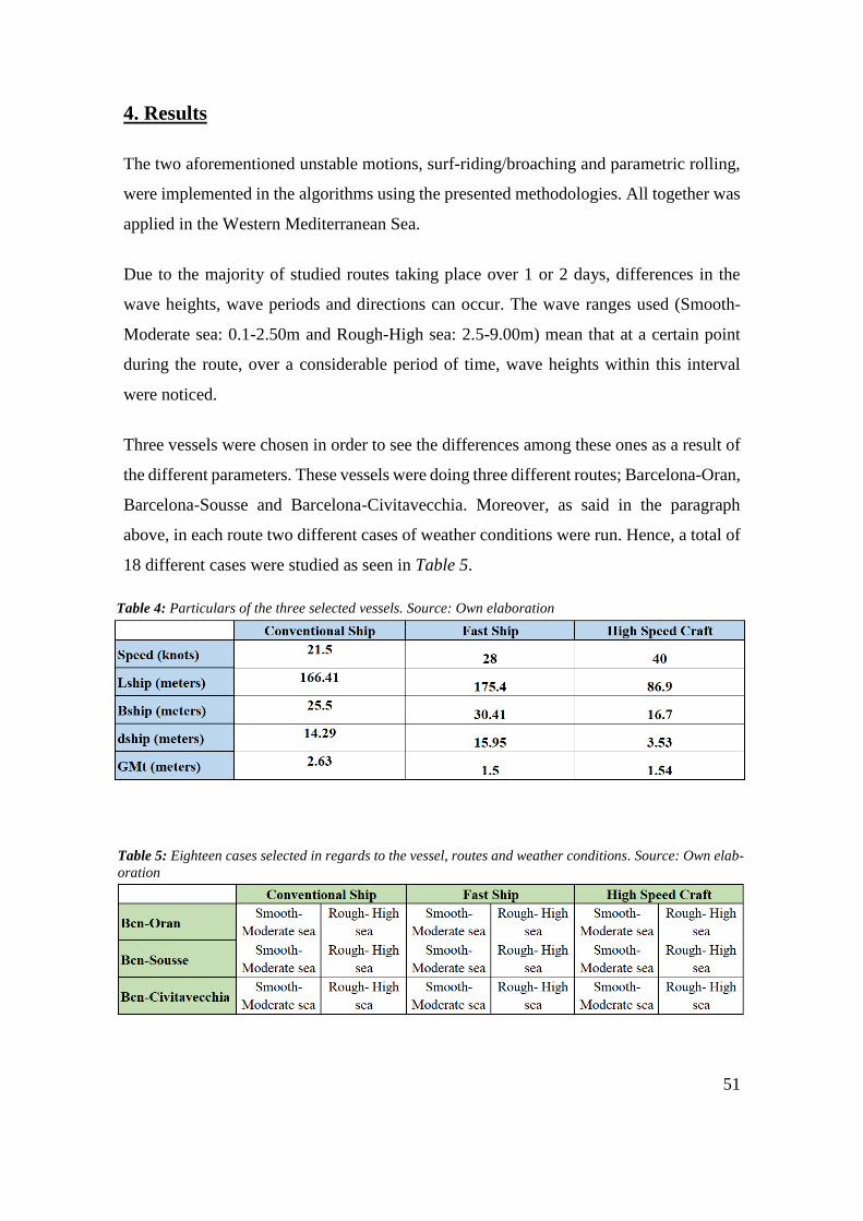
Three vessels were chosen in order to see the differences among these ones as a result of
the different parameters. These vessels were doing three different routes; Barcelona-Oran,
Barcelona-Sousse and Barcelona-Civitavecchia. Moreover, as said in the paragraph
above, in each route two different cases of weather conditions were run. Hence, a total of
18 different cases were studied as seen in Table 5.
Table 4: Particulars of the three selected vessels. Source: Own elaboration
Table 5: Eighteen cases selected in regards to the vessel, routes and weather conditions. Source: Own elab-
oration
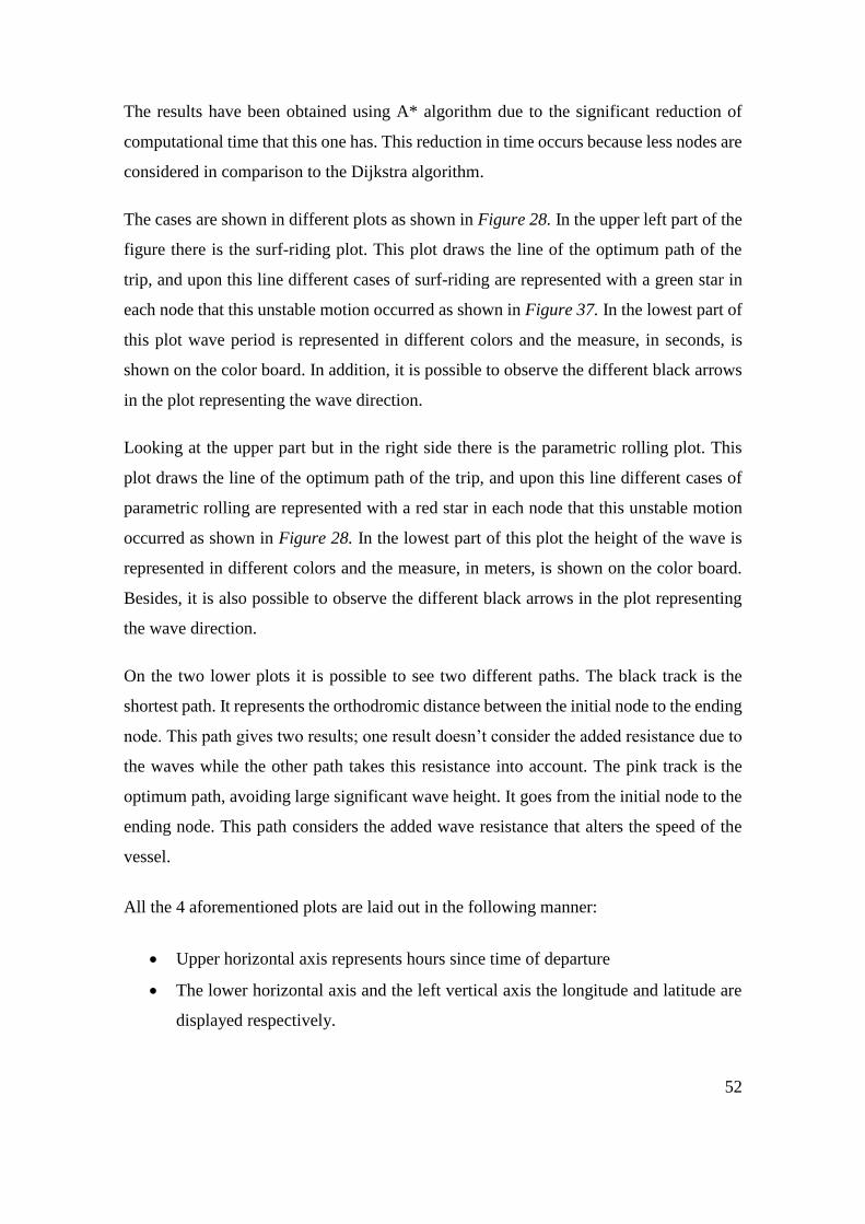
52
The results have been obtained using A* algorithm due to the significant reduction of
computational time that this one has. This reduction in time occurs because less nodes are
considered in comparison to the Dijkstra algorithm.
The cases are shown in different plots as shown in Figure 28. In the upper left part of the
figure there is the surf-riding plot. This plot draws the line of the optimum path of the
trip, and upon this line different cases of surf-riding are represented with a green star in
each node that this unstable motion occurred as shown in Figure 37. In the lowest part of
this plot wave period is represented in different colors and the measure, in seconds, is
shown on the color board. In addition, it is possible to observe the different black arrows
in the plot representing the wave direction.
Looking at the upper part but in the right side there is the parametric rolling plot. This
plot draws the line of the optimum path of the trip, and upon this line different cases of
parametric rolling are represented with a red star in each node that this unstable motion
occurred as shown in Figure 28. In the lowest part of this plot the height of the wave is
represented in different colors and the measure, in meters, is shown on the color board.
Besides, it is also possible to observe the different black arrows in the plot representing
the wave direction.
On the two lower plots it is possible to see two different paths. The black track is the
shortest path. It represents the orthodromic distance between the initial node to the ending
node. This path gives two results; one result doesn’t consider the added resistance due to
the waves while the other path takes this resistance into account. The pink track is the
optimum path, avoiding large significant wave height. It goes from the initial node to the
ending node. This path considers the added wave resistance that alters the speed of the
vessel.
All the 4 aforementioned plots are laid out in the following manner:
Upper horizontal axis represents hours since time of departure
The lower horizontal axis and the left vertical axis the longitude and latitude are
displayed respectively.

53
4.1. Conventional Ship (21.5 knots)
1st Case: Barcelona-Oran / Smooth-Moderate seas
As can be seen in Figure 28, surf-riding plot does not show signs of this unstable motion.
In parametric rolling plot there are just two nodes affected by this unstable motion. Wave
periods and wave heights around these nodes were about 4 seconds and 0.5-1 meters,
respectively. Wave direction average from 090 degrees with respect to the North.
Figure 28: Bcn-Oran/Smooth-Moderate sea/Conventional Ship. From left to right and from top to bottom: par-
ametric rolling plot; surf-riding plot; Wave height plot (10th hour of the trip); Wave period plot (10th hour of the
trip). Source: Own elaboration

54
Figure 29: Bcn-Oran/Rough-High sea/Conventional Ship. From left to right and from top to bottom: par-
ametric rolling plot; surf-riding plot; Wave height plot (19th hour of the trip); Wave period plot (19th hour
of the trip). Source: Own elaboration
2nd Case: Barcelona-Oran / Rough-High seas
As seen in Figure 29, the surf-riding and parametric rolling plots do not show any nodes
affected by these unstable motions. Wave periods and wave heights average were around
5 to 7 seconds and 6 to 10 meters, respectively. Wave direction average from the North.

55
3rd Case: Barcelona-Sousse / Smooth-Moderate seas
As can be seen in Figure 30, surf-riding and parametric rolling plots do not show any
nodes affected by these unstable motions. Wave periods and wave heights average were
around 3 to 5 seconds and 1.5 to 2.5 meters, respectively. Wave direction average from
090 to 135 degrees with respect to the North.
Figure 30: Bcn-Sousse/Smooth-Moderate sea/Conventional Ship. From left to right and from top to bottom:
parametric rolling plot; surf-riding plot; Wave height plot (28th hour of the trip); Wave period plot (28th hour
of the trip). Source: Own elaboration

56
4th Case: Barcelona-Sousse / Rough-High seas
As can be seen in Figure 31, surf-riding plot does not show signs of this unstable motion.
In parametric rolling plot there are five critical areas of this unstable motion. The master
should alter the course or reduce the speed. Wave periods and wave heights around these
nodes were about 6 to 9 seconds and 2 to 5 meters, respectively. Wave direction average
from 045 to 315 degrees with respect to the North.
Figure 31: Bcn-Sousse/Rough-High sea/Conventional Ship. From left to right and from top to bottom: parametric
rolling plot; surf-riding plot; Wave height plot (12th hour of the trip); Wave period plot (12th hour of the trip).
Source: Own elaboration
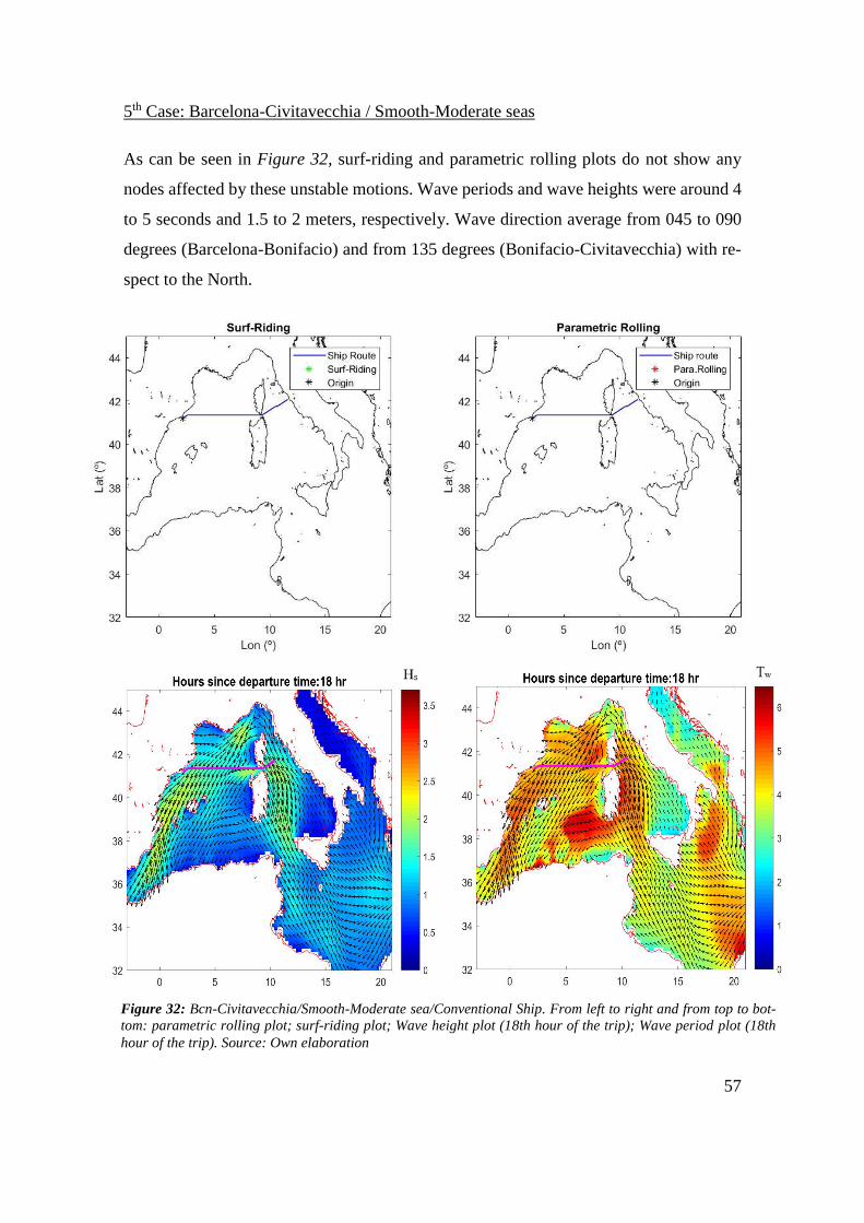
57
5th Case: Barcelona-Civitavecchia / Smooth-Moderate seas
As can be seen in Figure 32, surf-riding and parametric rolling plots do not show any
nodes affected by these unstable motions. Wave periods and wave heights were around 4
to 5 seconds and 1.5 to 2 meters, respectively. Wave direction average from 045 to 090
degrees (Barcelona-Bonifacio) and from 135 degrees (Bonifacio-Civitavecchia) with re-
spect to the North.
Figure 32: Bcn-Civitavecchia/Smooth-Moderate sea/Conventional Ship. From left to right and from top to bot-
tom: parametric rolling plot; surf-riding plot; Wave height plot (18th hour of the trip); Wave period plot (18th
hour of the trip). Source: Own elaboration
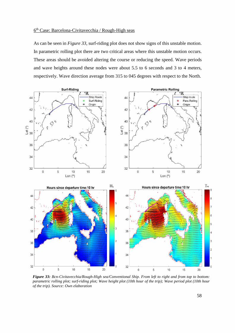
58
6th Case: Barcelona-Civitavecchia / Rough-High seas
As can be seen in Figure 33, surf-riding plot does not show signs of this unstable motion.
In parametric rolling plot there are two critical areas where this unstable motion occurs.
These areas should be avoided altering the course or reducing the speed. Wave periods
and wave heights around these nodes were about 5.5 to 6 seconds and 3 to 4 meters,
respectively. Wave direction average from 315 to 045 degrees with respect to the North.
Figure 33: Bcn-Civitavecchia/Rough-High sea/Conventional Ship. From left to right and from top to bottom:
parametric rolling plot; surf-riding plot; Wave height plot (10th hour of the trip); Wave period plot (10th hour
of the trip). Source: Own elaboration

59
4.2. Fast Ship (28 knots)
7th Case: Barcelona-Oran / Smooth-Moderate seas
As can be seen in Figure 34, surf-riding plot does not show signs of this unstable motion.
In parametric rolling plot there is one node affected by this unstable motion, this is prac-
tically insignificant due to the corresponding short period of time. Wave periods and wave
heights around the nodes were about 3 to 3.5 seconds and 0.5 meters, respectively. Waves
from 090 degrees with respect to the North.
Figure 34: Bcn-Oran/Smooth-Moderate sea/Fast Ship. From left to right and from top to bottom: parametric
rolling plot; surf-riding plot; Wave height plot (8th hour of the trip); Wave period plot (8th hour of the trip).
Source: Own elaboration.
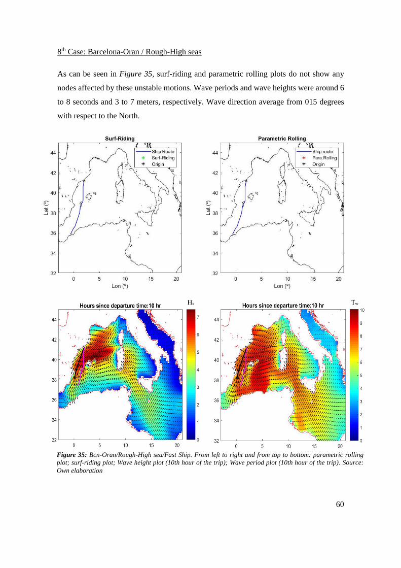
60
8th Case: Barcelona-Oran / Rough-High seas
As can be seen in Figure 35, surf-riding and parametric rolling plots do not show any
nodes affected by these unstable motions. Wave periods and wave heights were around 6
to 8 seconds and 3 to 7 meters, respectively. Wave direction average from 015 degrees
with respect to the North.
Figure 35: Bcn-Oran/Rough-High sea/Fast Ship. From left to right and from top to bottom: parametric rolling
plot; surf-riding plot; Wave height plot (10th hour of the trip); Wave period plot (10th hour of the trip). Source:
Own elaboration
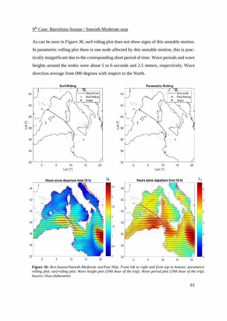
61
9th Case: Barcelona-Sousse / Smooth-Moderate seas
As can be seen in Figure 36, surf-riding plot does not show signs of this unstable motion.
In parametric rolling plot there is one node affected by this unstable motion, this is prac-
tically insignificant due to the corresponding short period of time. Wave periods and wave
heights around the nodes were about 5 to 6 seconds and 2.5 meters, respectively. Wave
direction average from 090 degrees with respect to the North.
Figure 36: Bcn-Sousse/Smooth-Moderate sea/Fast Ship. From left to right and from top to bottom: parametric
rolling plot; surf-riding plot; Wave height plot (19th hour of the trip); Wave period plot (19th hour of the trip).
Source: Own elaboration

62
10th Case: Barcelona-Sousse / Rough-High seas
As can be seen in Figure 37, surf-riding plot shows a considerable area next to Cagliari
where this unstable motion occurs. In parametric rolling plot, half of the route is plotted
in red. All these dangerous areas should be avoided altering the course or the speed. Wave
period in the parametric rolling area was between 6 and 9 seconds and wave height was
between 2.5 and 5 meters. Wave direction from 345 degrees in respect to the North around
the surf-riding area.
Figure 37: Bcn-Sousse/Rough-High sea/Fast Ship. From left to right and from top to bottom: parametric rolling
plot; surf-riding plot; Wave height plot (12th hour of the trip); Wave period plot (6th hour of the trip). Source:
Own elaboration
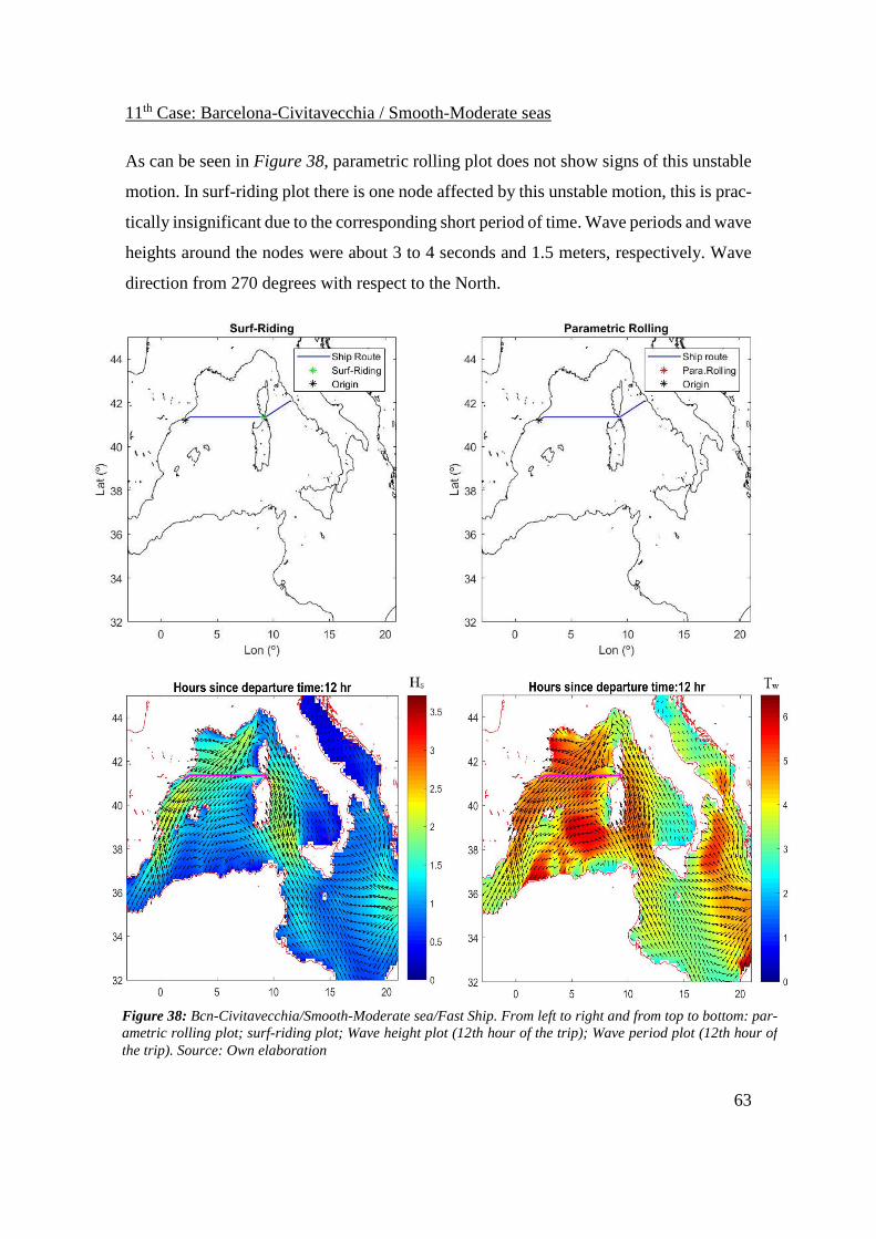
63
11th Case: Barcelona-Civitavecchia / Smooth-Moderate seas
As can be seen in Figure 38, parametric rolling plot does not show signs of this unstable
motion. In surf-riding plot there is one node affected by this unstable motion, this is prac-
tically insignificant due to the corresponding short period of time. Wave periods and wave
heights around the nodes were about 3 to 4 seconds and 1.5 meters, respectively. Wave
direction from 270 degrees with respect to the North.
Figure 38: Bcn-Civitavecchia/Smooth-Moderate sea/Fast Ship. From left to right and from top to bottom: par-
ametric rolling plot; surf-riding plot; Wave height plot (12th hour of the trip); Wave period plot (12th hour of
the trip). Source: Own elaboration

64
12th Case: Barcelona-Civitavecchia / Rough-High seas
As can be seen in Figure 39, surf-riding plot does not show signs of this unstable motion.
In parametric rolling plot there is a large area affected that should be avoided. Wave pe-
riods and wave heights around these nodes were about 6 to 8 seconds and 4 to 5.5 meters,
respectively. Wave direction from 315 degrees with respect to the North.
Figure 39: Bcn-Civitavecchia/Rough-High sea/Fast Ship. From left to right and from top to bottom: parametric
rolling plot; surf-riding plot; Wave height plot (5th hour of the trip); Wave period plot (5th hour of the trip).
Source: Own elaboration
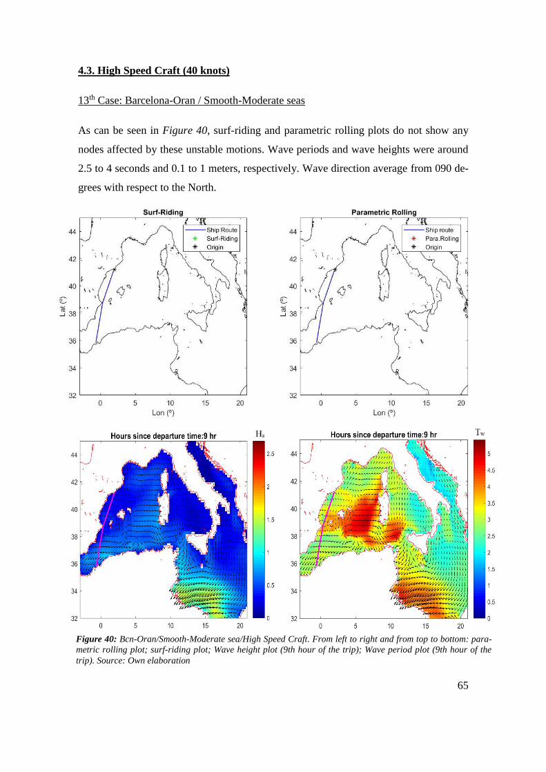
65
4.3. High Speed Craft (40 knots)
13th Case: Barcelona-Oran / Smooth-Moderate seas
As can be seen in Figure 40, surf-riding and parametric rolling plots do not show any
nodes affected by these unstable motions. Wave periods and wave heights were around
2.5 to 4 seconds and 0.1 to 1 meters, respectively. Wave direction average from 090 de-
grees with respect to the North.
Figure 40: Bcn-Oran/Smooth-Moderate sea/High Speed Craft. From left to right and from top to bottom: para-
metric rolling plot; surf-riding plot; Wave height plot (9th hour of the trip); Wave period plot (9th hour of the
trip). Source: Own elaboration
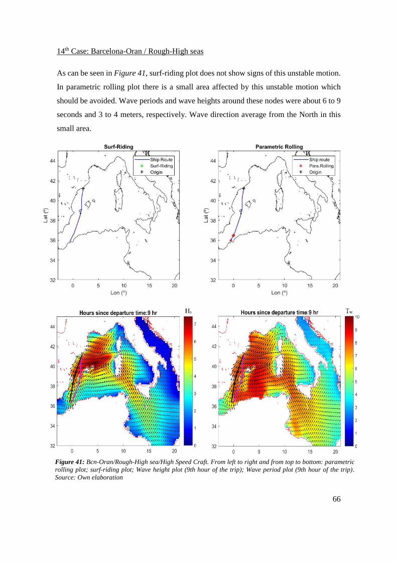
66
14th Case: Barcelona-Oran / Rough-High seas
As can be seen in Figure 41, surf-riding plot does not show signs of this unstable motion.
In parametric rolling plot there is a small area affected by this unstable motion which
should be avoided. Wave periods and wave heights around these nodes were about 6 to 9
seconds and 3 to 4 meters, respectively. Wave direction average from the North in this
small area.
Figure 41: Bcn-Oran/Rough-High sea/High Speed Craft. From left to right and from top to bottom: parametric
rolling plot; surf-riding plot; Wave height plot (9th hour of the trip); Wave period plot (9th hour of the trip).
Source: Own elaboration
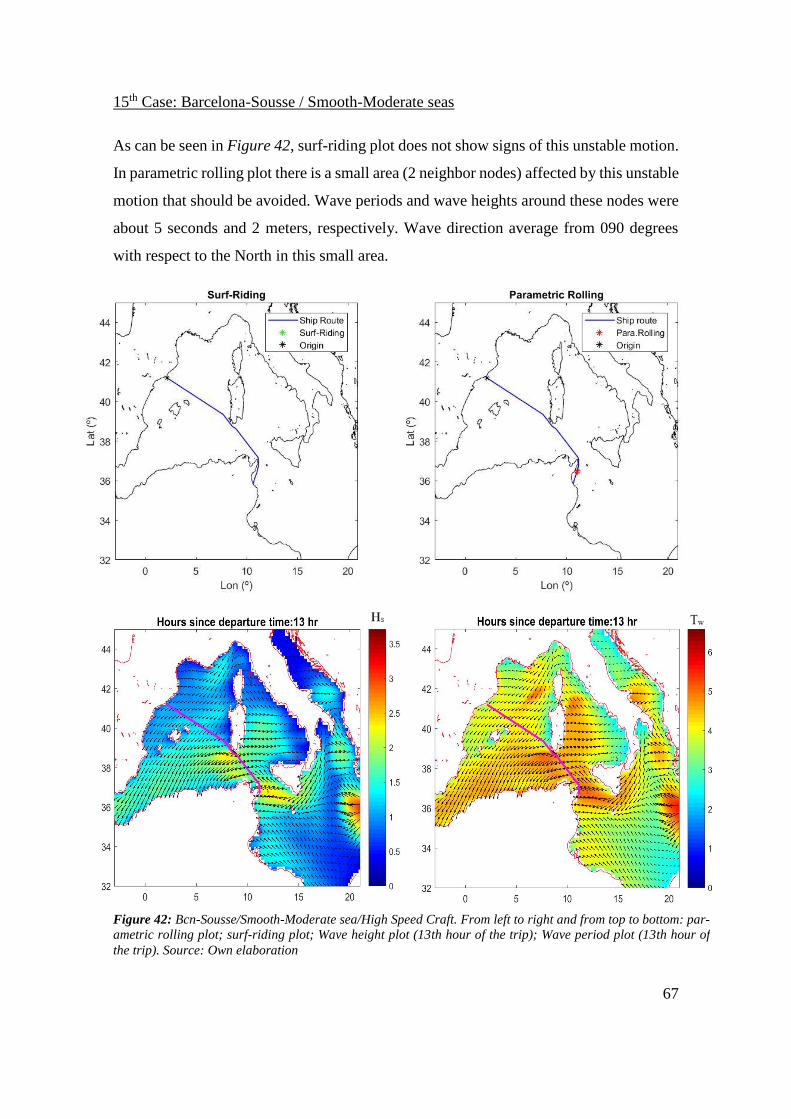
67
15th Case: Barcelona-Sousse / Smooth-Moderate seas
As can be seen in Figure 42, surf-riding plot does not show signs of this unstable motion.
In parametric rolling plot there is a small area (2 neighbor nodes) affected by this unstable
motion that should be avoided. Wave periods and wave heights around these nodes were
about 5 seconds and 2 meters, respectively. Wave direction average from 090 degrees
with respect to the North in this small area.
Figure 42: Bcn-Sousse/Smooth-Moderate sea/High Speed Craft. From left to right and from top to bottom: par-
ametric rolling plot; surf-riding plot; Wave height plot (13th hour of the trip); Wave period plot (13th hour of
the trip). Source: Own elaboration

68
16th Case: Barcelona-Sousse / Rough-High seas
This case is similar to 10th case. As can be seen in Figure 43, surf-riding plot shows a
considerable area next to Cagliari where this unstable motion occurs. In parametric rolling
plot, half of the route is plotted in red. All these dangerous areas should be avoided alter-
ing the course or the speed. Wave periods in the parametric rolling area were around 6 to
9 seconds and wave heights were around 2.5 to 5 meters. Wave direction from 345 de-
grees around the surf-riding area.
Figure 43: Bcn-Sousse/Rough-High sea/High Speed Craft. From left to right and from top to bottom: parametric
rolling plot; surf-riding plot; Wave height plot (6th hour of the trip); Wave period plot (6th hour of the trip).
Source: Own elaboration
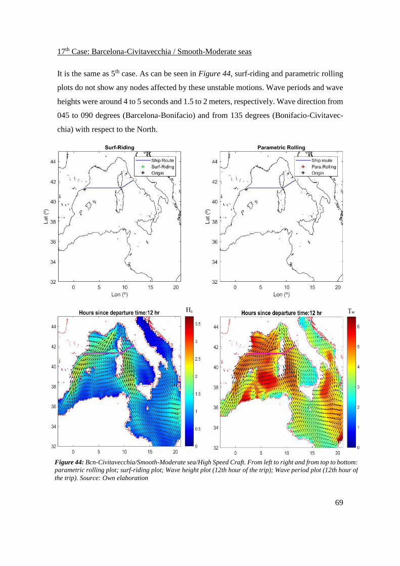
69
17th Case: Barcelona-Civitavecchia / Smooth-Moderate seas
It is the same as 5th case. As can be seen in Figure 44, surf-riding and parametric rolling
plots do not show any nodes affected by these unstable motions. Wave periods and wave
heights were around 4 to 5 seconds and 1.5 to 2 meters, respectively. Wave direction from
045 to 090 degrees (Barcelona-Bonifacio) and from 135 degrees (Bonifacio-Civitavec-
chia) with respect to the North.
Figure 44: Bcn-Civitavecchia/Smooth-Moderate sea/High Speed Craft. From left to right and from top to bottom:
parametric rolling plot; surf-riding plot; Wave height plot (12th hour of the trip); Wave period plot (12th hour of
the trip). Source: Own elaboration
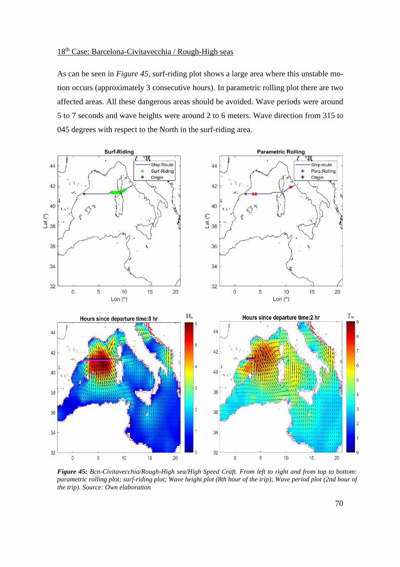
70
18th Case: Barcelona-Civitavecchia / Rough-High seas
As can be seen in Figure 45, surf-riding plot shows a large area where this unstable mo-
tion occurs (approximately 3 consecutive hours). In parametric rolling plot there are two
affected areas. All these dangerous areas should be avoided. Wave periods were around
5 to 7 seconds and wave heights were around 2 to 6 meters. Wave direction from 315 to
045 degrees with respect to the North in the surf-riding area.
Figure 45: Bcn-Civitavecchia/Rough-High sea/High Speed Craft. From left to right and from top to bottom:
parametric rolling plot; surf-riding plot; Wave height plot (8th hour of the trip); Wave period plot (2nd hour of
the trip). Source: Own elaboration
71
5. Conclusions
The presented work in this project is the study of the surf-riding/broaching and parametric
rolling and the implementation of these unstable motions in the ship-weather routing al-
gorithm SIMROUTEv2. A considerable quantity of cases was run in order to assure that
these dangerous phenomena can occur in Short Sea Shipping routes in the Western Med-
iterranean Sea.
Mediterranean Sea is thought to be an area with small wave periods, and this is what
might someone think that the occurrence of these unstable motions might almost be im-
possible. Considering the obtained results in section 4, it can be seen that 12 cases out of
18 at least one of the two phenomena happened.
During the results section, it was observed that the surf-riding unstable motion was im-
possible to occur with Conventional Ship. The phenomenon speed formula could not
comply with the vessel speed and length parameters. Parametric rolling was the only un-
stable motion that happened in different cases, highlighting the 4th case which has differ-
ent dangerous areas. In contrast, Fast Ship and High Speed Craft show different high-
lighted cases of surf-riding due to their speed is greater.
The different plots confirm the formulation of the phenomena; the two implemented un-
stable motions do not depend on the wave height. There is clear evidence in Smooth-
Moderate sea which is more difficult that these unstable motions occur, above all in par-
ametric rolling cases.
The greater the wave height the larger the wave period. Thus, implicitly, parametric roll-
ing is linked to the wave height. However, this does not mean that whenever there is a
large wave period parametric rolling occurs.
In regards to surf-riding, it occurs when the waves come from the aft or the quarters and
with a significant wave period. A clear example is case 18 which shows a large dangerous
of surf-riding due to wave height was 2 to 5 meters and wave period was 4 to 7 seconds.

72
Implementing the unstable motion formulas into the algorithm is an interesting tool in
order to know and avoid all the dangerous nodes from the route. Consequently, comply-
ing with IMO MSC.1/Circ.1228 will produce an enhancement of the safety on board, such
as crew members, passengers, cargo and ship integrity.
To sum up, in the Western Mediterranean Sea it is possible to find different cases which
surf-riding/broaching and parametric rolling occur. Hence, having this algorithm on board
would be ideal for the safety. Besides, the higher speed the bigger possibilities to have
surf-riding as long as wave direction come from the aft or the quarters of the vessel. In
regards to parametric rolling, there are more possibilities to occur with large wave peri-
ods.
Future work includes more implementation of the algorithm, taking into account external
factors such as wind and currents and avoiding the unstable motions recalculating the
optimum route. In addition, it proves beneficial to include one function for the fuel sav-
ings, as well as another function for the savings of the atmospheric pollutants. It will also
be useful to take into account the seasickness of the crew members and the passengers.

73
6. References
American Bureau of Shipping. (2004) Guide for the assessment of parametric roll reso-
nance in the design of container carriers. Houston, American Bureau of Shipping. Avail-
able from: https://www.boatdesign.net/attachments/assessment-of-parametric-roll-
pdf.93015/ [Accessed 15th February 2018].
Ananiev, D., (1966) On Surf-Riding in Following Seas. Leningrad, Transactions of
Krylov Society of Naval Architects.
Basiana, L. et al. (2017) Ship-weather routing applied to Short Sea Distances: study of
the feasibility of SIMROUTEv2 algorithm. In: Proceeding of the 18th Annual General
Assembly of the International Association of Maritime Universities, IAMU, 11-14 Octo-
ber 2017, Varna, Bulgaria. IAMU (1), pp. 330-340. Available from:
https://iamu2017.com/images/docs/proceeding/IAMU2017-volume1.pdf [Accessed 18th
February 2018].
Barrass, C. B. & Derrett, D. R., (2012) Ship Stability for Masters and Mates. Oxford,
Stanford Maritime Ltd.
Belenky V., et al. (2003) Probabilistic analysis of roll parametric resonance in head sea.
In: Proceedings of the 8th international conference on the stability of ships and ocean
vehicles, Madrid, Spain. Escuela Técnica Superior de Ingenieros Navales. pp 337–339.
Belenky, V. & Sevastianov, N. V., (2007) Stability and Safety of Ships: Risk of Capsizing.
Jersey City, The Society of Naval Architects and Marine Engineers.
Clark, I. C., (2005) Ship Dynamic for Mariners. London, The Nautical Institute.
Dechter, Rina & Pearl, Judea (1985) Generalized best-first search strategies and the opti-
mality of A*. Journal of the ACM. 32 (3), 505-536. Available from: http://citese-
erx.ist.psu.edu/viewdoc/download?doi=10.1.1.89.3090&rep=rep1&type=pdf [Accessed
26th February 2018].
Dijkstra, Edsger (1959) A note on two problems in connexion with graphs. Numerische
Mathematik. 1, 269-271. Available from: http://www-
74
m3.ma.tum.de/foswiki/pub/MN0506/WebHome/dijkstra.pdf [Accessed 25th February
2018].
Du Cane, P., Goodrich, J., (1962) The following sea, broaching and surging. London,
Transactions of the Royal Institution of Naval Architects.
European Commission White Paper (2011) Roadmap to a Single European Transport
Area - Towards a competitive and resource efficient transport system. Available from:
http://eur-lex.europa.eu/legal-con-
tent/EN/TXT/PDF/?uri=CELEX:52011DC0144&from=EN [Accessed 6th May 2018].
Eurostat (2017) Maritime transport statistics-short sea shipping of goods. Available at:
http://ec.europa.eu/eurostat/statistics-explained/index.php/Maritime_transport_statis-
tics_-_short_sea_shipping_of_goods [Accessed 1st April 2018].
Faltinsen, O., (1990) Sea Load son Ships and Offshore Structures. uque: Ola Trocoidal,
Movimientos y Esfuerzos. Cambridge, Cambridge University Press.
Grifoll, M. (2016). Ship routing applied at short sea distances. In: Proceedings of the 7th
International Conference on Maritime Transport, Barcelona, 27-29 June 2016, Barce-
lona, Spain. SERVICE POINT, pp. 240-245. Available from: https://upcom-
mons.upc.edu/handle/2117/89042 [Accessed 11th February 2018].
Hansen, S., Pedersen, E. (2008) On an Advanced Shipboard Information and Decision-
making System for Safe and Efficient Passage Planning. International Journal on Marine
Navigation and Safety of Sea Transportation, Vol. 2, No. 1: 69-73. Available from:
http://www.transnav.eu/Article_On_an_Advanced_Shipboard_Hansen,5,74.html [Ac-
cessed 10th January 2018].
IMO, (2007). Revised guidance to the master for avoiding dangerous situations in ad-
verse weather and sea conditions. London, International Maritime Organization.
MSC.1/Circ.1228. Available from: https://vp.imo.org/Customer/Subscrip-
tions/IMOVEGA/MemberPages/IMODocument.aspx?resultIndex=33&do-
cId=MSCC1228ACI&docDate=2017-11-27 [Accessed 3rd March 2018].
75
Kempf G. (1938) Die stabilitätsbeanspruchung der schiffe durch Wellen und
Schwingungen. Werft-Reederei-Hafen, Vol. 19: 200-202. Available from.
https://ci.nii.ac.jp/naid/20000873386/en/#cit [Accessed 16th February 2018].
Larsson, E., and Simonsen, M. H. (2014) DIRECT weather routing. Sweden, Chalmers
University of Technology. Available from: http://publications.lib.chalmers.se/rec-
ords/fulltext/205858/205858.pdf [Accessed 2nd February 2018].
Lu, R. et al. (2015) A semi-empirical ship operational performance prediction model for
voyage optimization towards energy efficient shipping. Ocean Engineering, Vol. 110,
Part B: 18-28. Available from: 10.1016/j.oceaneng.2015.07.042 [Accessed 24th March
2018].
Mannarini, G. et al. (2013) A Prototype of Ship Routing Decision Support System for an
Operational Oceanographic Service. The International Journal on Marine Navigation
and Safety of Sea Transportation, Vol. 7, No. 1: 53-59. Available from: http://www.trans-
nav.eu/Article_A_Prototype_of_Ship_Routing_Mannarini,25,408.html [Accessed 10th
January 2018].
Olivella, J., (1998) Teoría del Buque: Ola Trocoidal, Movimientos y Esfuerzos. Barce-
lona, Edicions UPC.
Padhy, C. et al. (2008) Application of wave model for weather routing of ships in the
North Indian Ocean. Nat. Hazards, Vol. 44, No. 4: 373–385. Available from:
https://link.springer.com/article/10.1007/s11069-007-9126-1 [Accessed 23rd February
2018].
Szłapczyńska, J., and Śmierzchalski, R. (2009) Multicriteria Optimisation in Weather
Routing. TransNav, the International Journal on Marine Navigation and Safety of Sea
Transportation, Vol. 3, No. 4: 393-400.
Takashima, K., Mezaoui, B., and Shoji, R. (2009) On the Fuel Saving Operation for
Coastal Merchant Ships using Weather Routing. The International Journal on Marine
Navigation and Safety of Sea Transportation, Vol. 3, No. 4: 401-406. Available from:
http://www.transnav.eu/Search_takashima.html [Accessed 5th March 2018].
76
Walden, D., (2003) The Bellman-Ford Algorithm and “distributed Bellman-Ford”. Avail-
able from: https://www.researchgate.net/publication/250014977_THE_BELLMAN-
FORD_ALGORITHM_AND_DISTRIBUTED_BELLMAN-FORD [Accessed 26th
February 2018].
Wei, Shao & Zhou, Peilin (2012) Development of a 3D Dynamic Programming Method
for Weather Routing. TransNav, the International Journal on Marine Navigation and
Safety of Sea Transportation, Vol. 6 No. 1: 79-85. Available from: http://www.trans-
nav.eu/Article_Development_of_a_3D_Dynamic_Wei,21,337.html [Accessed 10th Jan-
uary 2018].
Wendel, K., (1960) Safety from capsizing. Fishing boats of the world 2. London, Fishing
News Books Ltd.
Zachcial, Manfred (2001) Short Sea Shipping and intermodal transport. In: OECD (ed.)
Short Sea Shipping in Europe, Paris: OECD Publications, pp. 23-33.

77
7. Figure References
Figure 1: Basiana, L. et al. (2017) Ship-weather routing applied to Short Sea Distances:
study of the feasibility of SIMROUTEv2 algorithm. In: Proceeding of the 18th Annual
General Assembly of the International Association of Maritime Universities, IAMU, 11-
14 October 2017, Varna, Bulgaria. IAMU (1), pp. 330-340. Available from:
https://iamu2017.com/images/docs/proceeding/IAMU2017-volume1.pdf [Accessed 18th
February 2018].
Figure 2: The Law Offices of Countryman & McDaniel, (1998) The extreme state of
M/V APL China as she reaches Port of Seattle. Available from: http://www.cargo-
law.com/1998nightmare.html [Accessed 26th February 2018].
Figure 3: Clark, I. C., (2005) Ship Dynamic for Mariners. London, The Nautical Institute.
Figure 4: Clark, I. C., (2005) Ship Dynamic for Mariners. London, The Nautical Institute.
Figure 5: Clark, I. C., (2005) Ship Dynamic for Mariners. London, The Nautical Institute.
Figure 6: Own elaboration.
Figure 7: Clark, I. C., (2005) Ship Dynamic for Mariners. London, The Nautical Institute.
Figure 8: Clark, I. C., (2005) Ship Dynamic for Mariners. London, The Nautical Institute.
Figure 9: Clark, I. C., (2005) Ship Dynamic for Mariners. London, The Nautical Institute.
Figure 10: Clark, I. C., (2005) Ship Dynamic for Mariners. London, The Nautical Insti-
tute.
Figure 11: Umeda, N., (2015) Capsizing model experiments. Available from:
http://nrife.fra.affrc.go.jp/plant/kaiyou/capsizing-e.html [Accessed 13th March 2018]
Figure 12: Clark, I. C., (2005) Ship Dynamic for Mariners. London, The Nautical Insti-
tute.
78
Figure 13: IMO, (2007). Revised guidance to the master for avoiding dangerous situa-
tions in adverse weather and sea conditions. London, International Maritime Organiza-
tion. MSC.1/Circ.1228. Available from: https://vp.imo.org/Customer/Subscrip-
tions/IMOVEGA/MemberPages/IMODocument.aspx?resultIndex=33&do-
cId=MSCC1228ACI&docDate=2017-11-27 [Accessed 3rd March 2018].
Figure 14: Clark, I. C., (2005) Ship Dynamic for Mariners. London, The Nautical Insti-
tute.
Figure 15: Barrass, C. B. & Derrett, D. R., (2012) Ship Stability for Masters and Mates.
Oxford, Stanford Maritime Ltd.
Figure 16: IMO, (2007). Revised guidance to the master for avoiding dangerous situa-
tions in adverse weather and sea conditions. London, International Maritime Organiza-
tion. MSC.1/Circ.1228. Available from: https://vp.imo.org/Customer/Subscrip-
tions/IMOVEGA/MemberPages/IMODocument.aspx?resultIndex=33&do-
cId=MSCC1228ACI&docDate=2017-11-27 [Accessed 3rd March 2018].
Figure 17: Clark, I. C., (2005) Ship Dynamic for Mariners. London, The Nautical Insti-
tute.
Figure 18: Clark, I. C., (2005) Ship Dynamic for Mariners. London, The Nautical Insti-
tute.
Figure 19: Clark, I. C., (2005) Ship Dynamic for Mariners. London, The Nautical Insti-
tute.
Figure 20: Abadía digital, (2013) HMCS Iroquois. Available from: https://www.abadi-
adigital.com/proa-de-un-destructor-en-medio-de-una-tormenta/ [Accessed 23rd March
2018].
Figure 21: Petersen, K., (1977) “Stolt Surf” in the North Pacific. Available from:
http://global-mariner.com/index111TheStorm.html [Accessed 22nd March 2018].

79
Figure 22: IMO, (2007). Revised guidance to the master for avoiding dangerous situa-
tions in adverse weather and sea conditions. London, International Maritime Organiza-
tion. MSC.1/Circ.1228. Available from: https://vp.imo.org/Customer/Subscrip-
tions/IMOVEGA/MemberPages/IMODocument.aspx?resultIndex=33&do-
cId=MSCC1228ACI&docDate=2017-11-27 [Accessed 3rd March 2018].
Figure 23: Olivella, J., (1998) Teoría del Buque: Ola Trocoidal, Movimientos y Esfuer-
zos. Barcelona, Edicions UPC.
Figure 24: Own elaboration.
Figure 25: Own elaboration.
Figure 26: Padhy, C. et al. (2008) Application of wave model for weather routing of ships
in the North Indian Ocean. Nat. Hazards, Vol. 44, No. 4: 373–385. Available from:
https://link.springer.com/article/10.1007/s11069-007-9126-1 [Accessed 23rd February
2018].
Figure 27: Lu, R. et al. (2015) A semi-empirical ship operational performance prediction
model for voyage optimization towards energy efficient shipping. Ocean Engineering,
Vol. 110, Part B: 18-28. Available from: 10.1016/j.oceaneng.2015.07.042 [Accessed 24th
March 2018].
Figure 28: Own elaboration.
Figure 29: Own elaboration.
Figure 30: Own elaboration.
Figure 31: Own elaboration.
Figure 32: Own elaboration.
Figure 33: Own elaboration.
Figure 34: Own elaboration.

80
Figure 35: Own elaboration.
Figure 36: Own elaboration.
Figure 37: Own elaboration.
Figure 38: Own elaboration.
Figure 39: Own elaboration.
Figure 40: Own elaboration.
Figure 41: Own elaboration.
Figure 42: Own elaboration.
Figure 43: Own elaboration.
Figure 44: Own elaboration.
Figure 45: Own elaboration.

81
8. Table References
Table 1: Own elaboration.
Table 2: TRANSAS, (2014) MANOEUVRING BOOKLET V2.01 Mathematical model
of Ro-Ro Passenger Ferry 8 (Dis.21104t).
Table 3: Own elaboration.
Table 4: Own elaboration.
Table 5: Own elaboration.

82
Appendixes 1. Code Implementation
close all,clc,clear all
%%%TENACIA (21.5kt)
load('C:\Users\lluis\Desktop\CasosSimroutev2_Matlab\SIM-
ROUTE2_BCN_ORAN\out\BCN_ORAN112017012108.mat')
%%%TENACIA
Lship=166.41; %m
Bship=25.5; %m
dship=14.29; %m
tolerance=0.1;
GMt=2.63; %m
coef=0.373+(0.023*(Bship/dship))-0.043*(Lship/100);
T_roll=(2*coef*Bship)/(sqrt(GMt));%s
%Dirt relativa
k=0;
ntrip=length(nods_trip);
alfa=zeros(size(nods_trip));
angle_encounter=zeros(size(nods_trip));
for k=1:ntrip-1
nod_ini=nods_trip(k);
nod_end=nods_trip(k+1);
alfa(k+1)=ang_edge(nod_end,nod_ini);
angle_encounter(k+1)=dirt(k+1)- alfa(k+1);
end
%%%Surf-riding
k=0;
nodes_surf(1)=nods_trip(1);
for i=1:ntrip
velo=(1.8*sqrt(Lship))/cosd(180-dirt_relativa(i));
if (135 < dirt_relativa(i)) && (dirt_relativa(i) < 225) && (velo < v0)
k=k+1;
nodes_surf(k)=nods_trip(i);
else
end
end
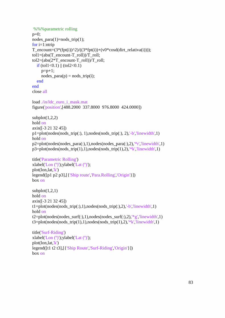
83
%%%parametric rolling
p=0;
nodes_para(1)=nods_trip(1);
for i=1:ntrip
T_encount=(3*(fpt(i))^2)/((3*fpt(i))+(v0*cosd(dirt_relativa(i))));
tol1=(abs(T_encount-T_roll))/T_roll;
tol2=(abs(2*T_encount-T_roll))/T_roll;
if (tol1<0.1) || (tol2<0.1)
p=p+1;
nodes_para(p) = nods_trip(i);
end
end
close all
load ./in/ldc_euro_i_mask.mat
figure('position',[488.2000 337.8000 976.8000 424.0000])
subplot(1,2,2)
hold on
axis([-3 21 32 45])
p1=plot(nodes(nods_trip(:), 1),nodes(nods_trip(:), 2),'-b','linewidth',1)
hold on
p2=plot(nodes(nodes_para(:),1),nodes(nodes_para(:),2),'*r','linewidth',1)
p3=plot(nodes(nods_trip(1),1),nodes(nods_trip(1),2),'*k','linewidth',1)
title('Parametric Rolling')
xlabel('Lon (º)');ylabel('Lat (º)');
plot(lon,lat,'k')
legend([p1 p2 p3],[{'Ship route','Para.Rolling','Origin'}])
box on
subplot(1,2,1)
hold on
axis([-3 21 32 45])
t1=plot(nodes(nods_trip(:),1),nodes(nods_trip(:),2),'-b','linewidth',1)
hold on
t2=plot(nodes(nodes_surf(:),1),nodes(nodes_surf(:),2),'*g','linewidth',1)
t3=plot(nodes(nods_trip(1),1),nodes(nods_trip(1),2),'*k','linewidth',1)
title('Surf-Riding')
xlabel('Lon (º)');ylabel('Lat (º)');
plot(lon,lat,'k')
legend([t1 t2 t3],[{'Ship Route','Surf-Riding','Origin'}])
box on
Copyright © 2022 FDOKUMEN

