Download - Unified Particle System for Multiple-fluid Flow and Porous ...

Unified Particle System for Multiple-fluid Flow and Porous Material

BO REN∗, Nankai University, ChinaBEN XU∗, Nankai University, ChinaCHENFENG LI, Swansea University, UK

Fig. 1. Selective filtering of a three-phase liquid mixture. The black liquid mixture flows through a vertical filter consisting of three layers of foam, eachabsorbing one fluid phase (red, green or blue). The porous foams turn into different colours as the mixture is selectively filtered.

Porous materials are common in daily life. They include granular material(e.g. sand) that behaves like liquid flow when mixed with fluid and foammaterial (e.g. sponge) that deforms like solid when interacting with liquid.The underlying physics is further complicated when multiple fluids interactwith porous materials involving coupling between rigid and fluid bodies,which may follow different physics models such as the Darcy’s law andthe multiple-fluid Navier-Stokes equations. We propose a unified particleframework for the simulation of multiple-fluid flows and porous materials.A novel virtual phase concept is introduced to avoid explicit particle statetracking and runtime particle deletion/insertion. Our unifiedmodel is flexibleand stable to cope with multiple fluid interacting with porous materials,and it can ensure consistent mass and momentum transport over the wholesimulation space.

CCS Concepts: • Computing methodologies→ Physical simulation.

Additional KeyWords and Phrases: porous media, fluid simulation, smoothedparticle hydrodynamics, virtual phase

ACM Reference Format:Bo Ren, Ben Xu, and Chenfeng Li. 2021. Unified Particle System for Multiple-fluid Flow and Porous Material. ACM Trans. Graph. 40, 4, Article 118 (Au-gust 2021), 14 pages. https://doi.org/10.1145/3450626.3459764∗Both authors contributed equally to the paper

Authors’ addresses: Bo Ren, Nankai University, 38 Tongyan Rd, Tianjin, 300350, China,[email protected]; Ben Xu, Nankai University, 38 Tongyan Rd, Tianjin, 300350, China,[email protected]; Chenfeng Li, Swansea University, Energy Safety ResearchInstitute, Bay Campus, Swansea, UK, [email protected].

Permission to make digital or hard copies of all or part of this work for personal orclassroom use is granted without fee provided that copies are not made or distributedfor profit or commercial advantage and that copies bear this notice and the full citationon the first page. Copyrights for components of this work owned by others than ACMmust be honored. Abstracting with credit is permitted. To copy otherwise, or republish,to post on servers or to redistribute to lists, requires prior specific permission and/or afee. Request permissions from [email protected].© 2021 Association for Computing Machinery.0730-0301/2021/8-ART118 $15.00https://doi.org/10.1145/3450626.3459764

1 INTRODUCTIONUnlike impermeable materials that can only interact with fluid flowsvia their surfaces, porous materials present a much stronger cou-pling when exposed to fluids, and the solid-fluid interaction takesplace both on their surfaces and inside their bodies. Phenomenasuch as water spilling out of a squeezed sponge, sea wave splash-ing on a sandy beach and cotton toy deforming when wetted aresome common examples of fluid flow interacting with porous media.These flow phenomena are far more complicated than the single-phase fluid flow in an open space, and they could involve manyphysical processes occurring simultaneously, such as liquid masstransport in the porous solid, absorption and emission on the solidsurface, hydrophobic and hydrophilic behaviours, capillary effectsand multiphase flows.

Simulations of single-fluid flow involving porous materials havebeen achieved using SPH (smoothed particle hydrodynamics) [Lenaertset al. 2008] and MPM (material point method) [Tampubolon et al.2017], producing impressive visual results. Despite the success, bothmethods face challenges associated with porous behaviours. UsingSPH, [Lenaerts et al. 2008] modelled the absorption and emissionof liquid by deleting/inserting fluid particles and tracking the fluidflow inside the solid particles. Thus, the simulator must constantlydelete/insert non-uniform SPH particles, which needs to be takenextra care of in calculation and implementation. A naive extensionof this approach to multiple fluid simulation will involve splittingthe fluid particles, since different fluid phase can potentially interactwith the solid differently. This will be an exhausting process produc-ing many fragmented particles. Alternatively, without splitting thefluid particle, one needs to cope with different mass and momentumtransports among various phases and maintain consistency for fluidparticles crossing the solid boundary. The MPM approach [Tampub-olon et al. 2017] uses two layers of grid to model sand and liquid

ACM Trans. Graph., Vol. 40, No. 4, Article 118. Publication date: August 2021.

https://doi.org/10.1145/3450626.3459764

https://doi.org/10.1145/3450626.3459764

118:2 • Bo Ren, Ben Xu, and Chenfeng Li

motions separately. For the sand-like porous material, a similar setof Navier-Stokes equations applies both to the pure liquid phaseand the solid-liquid mixture so that the focus is on the interactionbetween these two grid layers. However for other porous materialslike sponge, the fluid motions inside and outside the porous solid candiffer greatly (the flow in porous media obeys the Darcy’s law), andother physical processes like capillary effects may also be involved.Thus, it is not a trivial task to extend the capacity of the multi-gridMPM approach for generic porous media interacting with multiplefluids.

In this paper we present a universal SPH-based simulation schemefor multiple-fluid flows in porous materials. A special emphasis is onsponge-like materials where the internal flow follows Darcy’s lawand external flow is governed by the Navier-Stokes equations. In ourapproach, the internal and external flows are modelled uniformlyusing the volume fraction and a mixture model, avoiding constantparticle deletion and insertion. The new approach is able to capturea wide range of porous media flow phenomena, including poroe-lasticity, capillary effects and variable absorption in multiple-fluidenvironment. Our main contributions are:• A universal SPH framework for the simulation of multiple-fluid flow and sponge-like porous materials.• A novel concept of virtual phase to consistently capture thefluid flow when crossing porous surface and avoid runtimeparticle deletion/insertion.• A flexible constitutive modelling strategy based on the virtualphase concept, to support multiple fluid flow, porous mate-rial deformation and the coupled physics between fluid andporous solids.

The rest of paper is arranged as follows. Related works are brieflyrecapped in §2, after which the fundamental theories of our multiple-fluid SPH-based porous model is introduced in §3. We explain ourchoice of constitutive models in §4, and the designation of SPHdiscretization in §5. The simulation framework and implementationissues are explained in §6. A number of examples with differentvisual effects are presented in §7 to demonstrate the performance ofour model. Finally, concluding remarks and limitations are discussedin §8.

2 RELATED WORK

2.1 Simulation of Porous PhenomenaExplorations of porous behaviours are studied in a wide range ofgraphics works involving cloth, sand or mud, and volumetric solid.Some early research works focus on the absorption and diffusion ofliquid into solid. [Rungjiratananon et al. 2008] modelled the absorp-tion of water into sand using a combined SPH and DEM (discreteelement method) framework, which captures the cohesion changeduring sand wetting. [Huber et al. 2011] used Fick’s law to modelliquid diffusion inside wet cloth. Surface flow, absorption and in-cloth diffusion were combined to simulate thin-shell wetting in [Umet al. 2013], where changes of material properties due to wettingare considered.

More complex porous behaviours are also studied in the literature.In [Lenaerts et al. 2008], an SPH-based simulator was proposed forsimulating liquid flow in porous materials, where the Darcy flux is

introduced to model the absorbed flow behaviour. Their method canbe applied to a variety of scenarios involving porous media flow,but requires frequent particle deletion and insertion at solid surface.Later [Lenaerts and Dutre 2009] extended this model for wettedflows of granular materials, and [Lin 2015] combined it with two-way fluid-hair interactions. Fluid-hair interaction including liquidcapture and dripping was also studied in [Fei et al. 2017] using adimension-reduced model for thin liquid on hair cluster. In [Patkarand Chaudhuri 2013], absorbed liquid is stored on a triangle meshfor cloth or a tetrahedral mesh for volumetric solid and a diffusionequation is solved on the mesh structure. They also handled absorp-tion and dripping by a particle absorption and generating schemewith an integrated SPH simulator for liquid flow outside the solidregion. Recently, [Fei et al. 2018] used a set of saturated continuityequations for porous flow inside fabric porous materials, which sup-ports anisotropic fabric microstructure and its nonlinear drag andpore pressure forces. Similarly, an integrated bulk liquid simulator isused in their work and a particle absorbing and generating schemeis designed for liquid capturing and dripping. In [Zheng et al. 2020]miscible and immiscible diffusion models are considered to simulatemulti-solvent stains on textile. [Ding et al. 2019] combined liquiddiffusion and gas stress in a thermomechanical porous model forbaking and cooking effect simulation.As a special case of porous media flow, the granular flow has

been receiving increasing attention from the graphics community inrecent years. [Baek et al. 2015] classified mud particles into differentsizes and solved respective suspension particle motion for muddyflows. [Yan et al. 2016; Yang et al. 2017] used the volume fraction todescribe the concentration of granular material in the liquid, and theporous behaviour was treated similarly to solid dissolving. [Gao et al.2018; Tampubolon et al. 2017] used MPM to simulate granular sandflows in water, and two background grids were used for the fluid andsand phase separately, with the interaction between phases handledthrough a momentum exchange term. This approach can handlelarge scenarios effectively, but does not cover wider physics, e.g.capillary phenomena. In addition, the previous research works ofgranular materials usually use Navier-Stokes equations for both thepure liquid phase and the solid-liquid mixture, while the internalflow could be better captured by using Darcy’s law in a generalporous medium. Our approach does not require the physics laws tobe the same inside and outside the solid, and at the same time doesnot need to frequently delete and generate particles at solid surface.

Porous have been studied using different models and theories inrelevant fields. Some approaches explicitly model the detailed geom-etry of porous materials [Berrone et al. 2017; Hilfer 2006; Wu et al.2004], where a porous material is treated as a network of connectedpore spaces and the fluid flow in the pore-space network is trackedby carefully calculating the interactions between pore surface andfluid. In [Jin et al. 2017] porous permeability was modelled by thefractal properties of the porous media. We refer to [Fei et al. 2018]for a more comprehensive summary on modelling approaches ofporous media.


Unified Particle System for Multiple-fluid Flow and Porous Material • 118:3

2.2 SPH method.We have integrated our models with the SPH method [Becker andTeschner 2007a; Monaghan 1994; Müller et al. 2003] to establisha unified particle system for multiple-fluid flow and porous mate-rial. Thus, in order to place the present work in the right researchcontext, the most relevant research works on SPH are also brieflyrecapped here. [Aly and Raizah 2018; Ihmsen et al. 2014a] developedpressure projection schemes are developed for SPH fluid simula-tion, and [Bender and Koschier 2016; Macklin and Müller 2013;Solenthaler and Pajarola 2009] ensured the incompressibility byprediction-correction schemes. Solid-fluid boundary coupling isalso comprehensively studied in the SPH literature. By sampling thesolid surface with particles, [Akinci et al. 2012] proposed a versatilerigid-fluid coupling method. In [Band et al. 2018a], by integratingwith the implicit incompressible SPH (IISPH), better boundary parti-cle pressure calculation that ensures physically meaningful pressuregradient was achieved. Recently, [Band et al. 2018b] adopted a mov-ing least square technique to further reduce false velocity artifacts atthe boundary. On the other hand, stability issues were also studiedusing density maps [Bender et al. 2020; Koschier and Bender 2017]or an interleaved velocity update iterative solver [Gissler et al. 2019].The above incompressibility and solid-liquid coupling studies are allfor single-fluid flow and the discussion on miscible multiple fluidsis sparse. For other SPH research topics, we refer to [Ihmsen et al.2014b] and [Koschier et al. 2019], which provide thorough surveysof the graphics SPH literature.

2.3 Multiple fluid simulation.The multiple fluid simulation has been studied by the graphics com-munity for over a decade. Several grid-based simulators were devel-oped for interfacial flow [Hong and Kim 2005; Kim 2010; Losassoet al. 2006], where the interfaces between different phases are ex-actly tracked. Volume fraction based grid solvers were proposedin [Bao et al. 2010; Kang et al. 2010], where miscible phases aresimulated. [Nielsen and Osterby 2013] solved the full two-fluidNavier-stokes equations implicitly providing vivid visual appear-ance of water sprays. The volume fraction concept has been widelyadopted in recent particle-based frameworks. SPH-based mixture-model multiple-fluid simulator was proposed by [Ren et al. 2014; Yanet al. 2016] where a phase-wise drift velocity is essential for variousmixing/unmixing effects in multiple-fluid flow including solid. Bycombining Navier-Stokes equation with a phase-field model, [Yanget al. 2017, 2015] proposed an energy-based multiple fluid solverthat also captures distillation effects. The material point method(MPM) has shown its effectiveness in multiple fluid simulations aswell. [Yan et al. 2018] proposed a MPM-based multiple fluid solverto model interactions between multiple fluid and solid phases. [Gaoet al. 2018; Tampubolon et al. 2017] targeted granular flows using atwo-layer grid for solid and liquid phases. In all these studies, thesolid phase is either impermeable or follows the same fluid govern-ing equations after dissolving. To simulate sponge-like materials,our work allows flows inside and outside the solid to follow differentphysics laws.Fluid mixture simulations are also studied in many other works

such as in surface flows [Ren et al. 2018b] and viscosity blending

model for shear thinning fluids [Nagasawa et al. 2019]. We refer to[Ren et al. 2018a] for a more comprehensive summary of graphicsmultiple-fluid studies.

3 UNIVERSAL SPH MODEL FOR MULTIPHASE FLOWAND POROUS MATERIAL

3.1 Problem FormulationA simulation space involving porous materials and fluid flows can benaturally divided into two parts, i.e. the “inner” and “outer” regionsof the porous material, and the fluid flow travels in or between thesetwo regions. In our universal SPH model, we consider a generalcase where there are three coupled physical mechanisms, i.e. poroussolid motion, inner fluid transport, and outer fluid motion, and theymay follow different physical laws. Therefore, we consider threesets of governing equations that describes each of the three parts inthe coupled physics of multiple-fluid flow and porous materials.First, for fluid flow inside the porous material, we use Darcy’s

law [Darcy 1856] to simulate the flow motion. Specifically, the in-stantaneous flow rate, i.e. Darcy flux, in a homogeneous permeablematerial is determined by

q𝑘 = −k𝑤𝑘

`𝑘· ∇𝑝𝑝𝑜𝑟𝑒𝑠 , (1)

where the subscript 𝑘 denotes the 𝑘-th fluid phase, q𝑘 Darcy flux ofthe phase 𝑘 , k𝑤𝑘 the permeability tensor, `𝑘 the fluid viscosity, andthe pore pressure 𝑝𝑝𝑜𝑟𝑒 represents the pressure of fluid in the porespace. Based on experiments and the homogenization of Navier-Stokes equations, the Darcy’s law describes porous flow in poroussolids. The pore pressure in Darcy’s law is determined by the statesof solid and locally absorbed fluid, and represented by Eq. (1) itdrives the absorbed fluid from the region with pore pressure to theregion with low pore pressure.Next, for fluid flow outside the porous material, we adopt the

multiple-fluid mixture model [Ren et al. 2014; Yan et al. 2016]:

𝐷𝛼𝑘

𝐷𝑡= −𝛼𝑘∇ · u𝑚 − ∇ · (𝛼𝑘 u𝑚𝑘 ) (2)

𝜕

𝜕𝑡u𝑚 + (u𝑚 · ∇)u𝑚 = g + a𝑝𝑟𝑒𝑠𝑠 + a𝑜𝑡ℎ𝑒𝑟 , (3)

where 𝛼𝑘 is the volume fraction of phase 𝑘 , u𝑚 and u𝑚𝑘 are themixture velocity and drift velocity of the phase 𝑘 , and g, a𝑝𝑟𝑒𝑠𝑠 anda𝑜𝑡ℎ𝑒𝑟 denote the gravity, pressure, and other influencing factors(viscosity, etc.), respectively. We use the tilde notation in the aboveequations to distinguish them from the “virtual-phase” quantitieswe are going to introduce. The mixture model expresses the conti-nuity and momentum equations through aggregate values averagedover the local volume, which for SPH is the particle. It can capturethe phase-wise velocity difference, but only needs to solve for theparticle velocity by analytically computing the drift velocities. Inthe mixture model solver, standard particle advance scheme canbe used and the phase volume fraction changes within a particle isautomatically handled by the continuity equation.Finally, for the porous solid, we adopt the elastic solid model

[Peer et al. 2018] which is a corotated material model. The strain



tensor 𝜖 is expressed as:

𝜖 =12(F + F𝑇 ) − I, (4)

where F is the deformation gradient tensor and I is the identitymatrix. To take into account the effect of pore pressure on thedeformation of solid and inspired by [Lenaerts et al. 2008], we adda term −[𝑝𝑝𝑜𝑟𝑒 I to their stress tensor and express the stress tensorP as follows:

P = 2a𝜖 + _tr(𝜖)I − [𝑝𝑝𝑜𝑟𝑒𝑠 I, (5)where a , _ are Lamé parameters and [ is a solid constant. The lastterm was introduced in [Lenaerts et al. 2008] and represents theeffect of pore pressure, i.e. absorbing fluid will let the solid expand.

In our study, the above governing equations are discretized usingtwo kinds of particles, i.e. solid particles representing the poroussolid and fluid particles representing fluid flow. A discretizationproblem emerges from the inner/outer fluid coupling, i.e. transitionbetween outer and inner fluids. Previous approaches [Fei et al. 2018;Lenaerts et al. 2008; Patkar and Chaudhuri 2013] typically use dif-ferent solvers for inner and outer regions, with the SPH particlesrepresenting the fluid placed only in the outer region. As a result,SPH particles are deleted or inserted when fluid passes throughthe surface of porous material. This method becomes exhaustingfor multiple fluid simulation when different fluid phases interactwith the porous solid in different ways, producing many particleswith non-uniform sizes near the porous solid interface. On the con-trary, we design our approach to let fluid particles remain in thesimulation when they cross the surface of porous material (whetherthrough absorbing or emitting). No particle gets deleted or insertedat interface crossing. This is achieved by a novel extension of thevolume fraction representation and the mixture model [Ren et al.2014], which in turn leads to a universal simulation framework.More details are explained in §3.2.

3.2 Virtual Phase for Fluid ParticlesThe above governing equations can be solved individually withexisting methods, but they become strongly coupled near the surfaceof porous material, greatly increasing the solution complexity. Wepropose the concept of virtual phase to handle the state change offluid particles crossing the interface and the associated mass andmomentum transport in a uniformmanner, thereby avoiding explicitstate tracking and runtime particle deletion/insertion.

Specifically, we assign each fluid particle with two virtual phases𝛼𝑘 and 𝛽𝑘 , which represent the volume fractions of the phase 𝑘in the outer and inner regions, respectively, and they satisfy therelation

∑𝑘 (𝛼𝑘 + 𝛽𝑘 ) = 1. Thus,

∑𝑘 𝛼𝑘 = 1 indicates that the fluid

particle locates outside the porous material,∑𝑘 𝛽𝑘 = 1 indicates

that the particle locates inside the porous material, and non-zero𝛼 and 𝛽 values indicate that the fluid particle is near the surfaceof porous material. Consider an example where a fluid particle ata two-phase state is moving from the outer region into the innerregion, but only one fluid phase can be absorbed into the porousmaterial while the other cannot. The mass transport, momentumand position change of this fluid particle are affected by all materialphases, each in turn may have separate inner and outer fractionsfollowing different laws in the inner and outer regions. The virtual

phase concept distinguishes these fractions and virtual phases canfollow separate governing equations. The virtual phases have aproperty that 𝛼𝑘 and 𝛽𝑘 can be transferred, by absorption or othermechanisms, near the surface of porous material without violatingthemass conservation law, but volume fractions between real phasescannot be simply transferred.Aided by the virtual fraction concept, the inner and outer fluid

particle dynamics can be solved in a universal manner using anextended mixture model. The complex inner-outer state transitionunder different phase behaviour in relation to the porous solid isthen handled by solving continuity equations in the multiple-fluidmodel. The universal equations for all fluid particles are:

𝐷𝛼𝑘

𝐷𝑡= −𝛼𝑘∇ · u𝑚 − ∇ · (𝛼𝑘u𝑚𝑘,𝛼 ) + ∇ · Dk (6)

𝐷𝛽𝑘

𝐷𝑡= −𝛽𝑘∇ · u𝑚 − ∇ · (𝛽𝑘u𝑚𝑘,𝛽 ) − ∇ · Dk (7)

𝜕

𝜕𝑡u𝑚 + (u𝑚 · ∇)u𝑚 = g + a𝑝𝑟𝑒𝑠𝑠 + a𝑝𝑜𝑟𝑒 + a𝑐𝑎𝑝 + a𝑜𝑡ℎ𝑒𝑟 , (8)

where 𝛼𝑘 and 𝛽𝑘 are the outer and inner volume fractions of phase 𝑘 ,u𝑚 and u𝑚𝑘,𝛼 , u𝑚𝑘,𝛽 are the fluid-particle velocity and drift velocityof the outer and inner fluids, D𝑘 is the absorption flux and ∇ · D𝑘 isan absorption source term, and g, a𝑝𝑟𝑒𝑠𝑠 , a𝑝𝑜𝑟𝑒 , a𝑐𝑎𝑝 , a𝑜𝑡ℎ𝑒𝑟 denotethe accelerations from gravity, pressure, pore pressure, capillaryforces and other factors (e.g. viscosity), respectively.

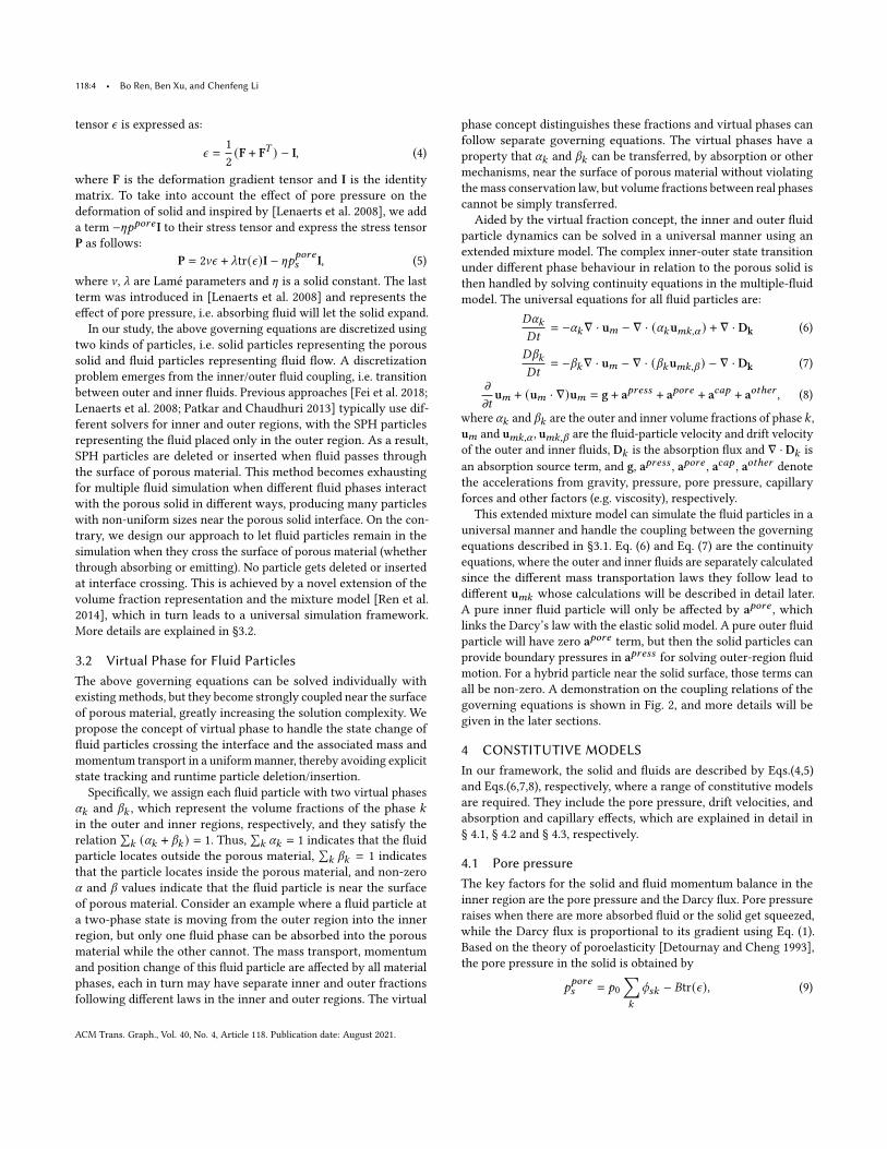
This extended mixture model can simulate the fluid particles in auniversal manner and handle the coupling between the governingequations described in §3.1. Eq. (6) and Eq. (7) are the continuityequations, where the outer and inner fluids are separately calculatedsince the different mass transportation laws they follow lead todifferent u𝑚𝑘 whose calculations will be described in detail later.A pure inner fluid particle will only be affected by a𝑝𝑜𝑟𝑒 , whichlinks the Darcy’s law with the elastic solid model. A pure outer fluidparticle will have zero a𝑝𝑜𝑟𝑒 term, but then the solid particles canprovide boundary pressures in a𝑝𝑟𝑒𝑠𝑠 for solving outer-region fluidmotion. For a hybrid particle near the solid surface, those terms canall be non-zero. A demonstration on the coupling relations of thegoverning equations is shown in Fig. 2, and more details will begiven in the later sections.

4 CONSTITUTIVE MODELSIn our framework, the solid and fluids are described by Eqs.(4,5)and Eqs.(6,7,8), respectively, where a range of constitutive modelsare required. They include the pore pressure, drift velocities, andabsorption and capillary effects, which are explained in detail in§ 4.1, § 4.2 and § 4.3, respectively.

4.1 Pore pressureThe key factors for the solid and fluid momentum balance in theinner region are the pore pressure and the Darcy flux. Pore pressureraises when there are more absorbed fluid or the solid get squeezed,while the Darcy flux is proportional to its gradient using Eq. (1).Based on the theory of poroelasticity [Detournay and Cheng 1993],the pore pressure in the solid is obtained by

𝑝𝑝𝑜𝑟𝑒𝑠 = 𝑝0

∑𝑘

𝜙𝑠𝑘 − 𝐵tr(𝜖), (9)



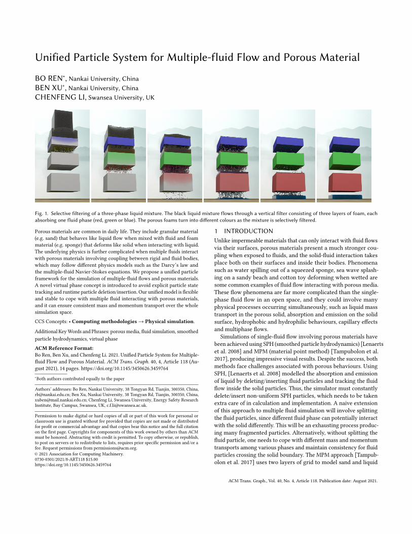
Fig. 2. The coupling betweenmultiple fluids and porous solid. The governingequations for solid, inner fluid and outer fluid are represented by the red,green and blue disks, respectively, and the arrows between them indicatethe physical interactions involved in the coupling.

where 𝑝0 is the rest pore pressure, tr(𝜖) the volumetric strain, 𝐵 aBiot’s ratio constant determined by the Biot’s modulus and the Biot’scoefficient of the solid, and 𝜙𝑠𝑘 the phase 𝑘’s absorbed volume rate(see § 5 for details). The above pore pressure is computed on the solidparticles and can be directly used for solid motion computations.We then compute its gradient on fluid particles for the Darcy fluxin Eq. (1) by collecting nearby solid particle information.The pore pressure affects the behaviour of solid as described in

Eq. (5), and it is also a driving force for the fluid flow inside solid. Apore pressure is exerted to the internal fluid and if no other forces arepresent, its contribution ends at the next simulation step, makingthe relative fluid-solid velocity u𝑟𝑘 agree with the Darcy flux inEq. (1) through u𝑟𝑘 = q𝑘/𝑒 , where 𝑒 is called porosity describingthe fraction of void volume over the total volume. We thus add aterm a𝑝𝑜𝑟𝑒 in Eq. (8) to model this force source in the simulation ofinner and outer fluid. Specifically, we use

a𝑝𝑜𝑟𝑒 =∑𝑘

𝛽𝑘

𝜌 𝑓𝑚Δ𝑡(𝜌𝑘u𝛽𝑘 − 𝜌𝛽𝑚u𝑚), (10)

where 𝜌𝛽𝑚 =∑𝑘

𝛽𝑘𝜌𝑘∑𝑘′ 𝛽𝑘′

is the inner rest density, u𝛽𝑘 = u𝑟𝑘 + u𝑠is the world-coordinate phase velocity of phase 𝑘 , u𝑠 is the solidvelocity, 𝜌 𝑓𝑚 =

∑𝑘 (𝛼𝑘 + 𝛽𝑘 )𝜌𝑘 is the aggregate density of fluid

particle. The derivation is provided in Appendix B.

4.2 Drift VelocitiesThe drift velocity represents the relative velocity between the localphase and the aggregate mixture particle, and it plays a key role incapturing the multiple fluid behaviours in the mixture model [Renet al. 2014; Yan et al. 2016]. By taking into account the drift velocityin the continuity equation, the mixture model can automaticallyhandle the volume fraction changes of each phase within a particleduring bulk flow motion. This feature is beneficial to our problem

in that the virtual phase volume fractions can be similarly solvedby Eqs.(6,7) without explicitly distinguishing inner or outer fluidparticles in solving the bulk fluid motion.

We extend the drift velocity from [Ren et al. 2014; Yan et al. 2016]to cope with the porous fluid simulation. For an outer fluid virtualphase 𝛼𝑘 , its drift velocity is:

u𝑚𝑘,𝛼 =𝜏 (𝜌𝑘 −∑𝑘′

𝑐𝛼𝑘′𝜌𝑘′ )a − 𝜏 (∇𝑝𝑘 −∑𝑘′

𝑐𝛼𝑘′∇𝑝𝑘′ )−

𝜎 ( ∇𝛼𝑘𝛼𝑘−∑𝑘′

𝑐𝛼𝑘′∇𝛼𝑘′𝛼𝑘′) − 𝜑 (∇𝑝𝑝𝑜𝑟𝑒

𝑘−∑𝑘′

𝑐𝛼𝑘′∇𝑝𝑝𝑜𝑟𝑒

𝑘′ ),(11)

where 𝑐𝛼𝑘 =𝛼𝑘𝜌𝑘∑

𝑘′ 𝛼𝑘′𝜌𝛼𝑚denotes the outer mass fraction, 𝜌𝛼𝑚 =∑

𝑘𝛼𝑘𝜌𝑘∑𝑘′ 𝛼𝑘′

denotes the outer mixture density, a = 𝑔 − (u𝑚 · ∇)u𝑚 −𝜕u𝑚𝜕𝑡 , and 𝜏 , 𝜎 and 𝜑 are constant weight factors, ∇𝑝𝑝𝑜𝑟𝑒

𝑘is the

gradient of pore pressure of the liquids, which can be phase-specificsince different phases usually are absorbed differently. Eq. (11) differsfrom the original drift velocity only by the last term, which modelsthe sucking or propelling effects due to absorption or emission nearthe porous solid surface. The calculation of ∇𝑝𝑝𝑜𝑟𝑒

𝑘will be explained

in more details in §4.3 and §5.The inner fluid virtual phase 𝛽𝑘 obeys the Darcy’s law within the

porous solid, and it does not have the same hydrodynamic pressureas in the outer region. As the pore pressure in the inner region playsthe same role as the hydrodynamic pressure of fluids in the outerregion, we replace the second term of the original drift velocityequation to form our inner-fluid drift velocity model:

u𝑚𝑘,𝛽 =𝜏 (𝜌𝑘 −∑𝑘′𝑐𝛽𝑘′𝜌𝑘′)a − 𝜏 ′(q𝑘 −

∑𝑘′𝑐𝛽𝑘′q𝑘′)−

𝜎 ′( ∇𝛽𝑘𝛽𝑘−∑𝑘′𝑐𝛽𝑘′∇𝛽𝑘′𝛽𝑘′),

(12)

where 𝑐𝛽𝑘 denote the inner mass fraction (corresponding to 𝑐𝛼𝑘defined in Eq. (11)), and 𝜏 ′, 𝜎 ′ are constant weight factors (the apos-trophe indicates that they may differ from those in Eq. (11) due todifferent environment settings of inner and outer regions). Note thatit does not matter in Eq. (12) whether q𝑘 is computed from Eq. (1)(i.e. in the local solid coordinate) or in the world coordinate. As longas the solid porosity is homogeneous, since

∑𝑘 𝑐𝛽𝑘 = 1, we can

obtain the same result using q𝑘 calculated under either coordinate.

4.3 Absorption and Capillary EffectsFluid absorption and emission can occur between fluid and poroussolid. To capture these effects, we assume that the outer fluid alsohas a phase-wise constant pore pressure 𝑝0𝑘 that corresponds todifferent absorption tendencies. When the outer pore pressure isgreater than the inner pore pressure, the fluid will get absorbedand a liquid particle may flow into the solid, and vice versa. On theother hand, inside the porous solid, we take a simplification andassume the pore pressure is unified across phases and related to theabsorbed fluid volume and volumetric strain by Eq. (9).Similar to the Darcy flux calculation in Eq. (1), we compute the

gradient of pore pressure to obtain the absorption flux:

D𝑘 = −𝐾 kwk`𝑘(𝛼𝑘 + 𝜙𝑠𝑘 )∇𝑝

𝑝𝑜𝑟𝑒

𝑘, (13)



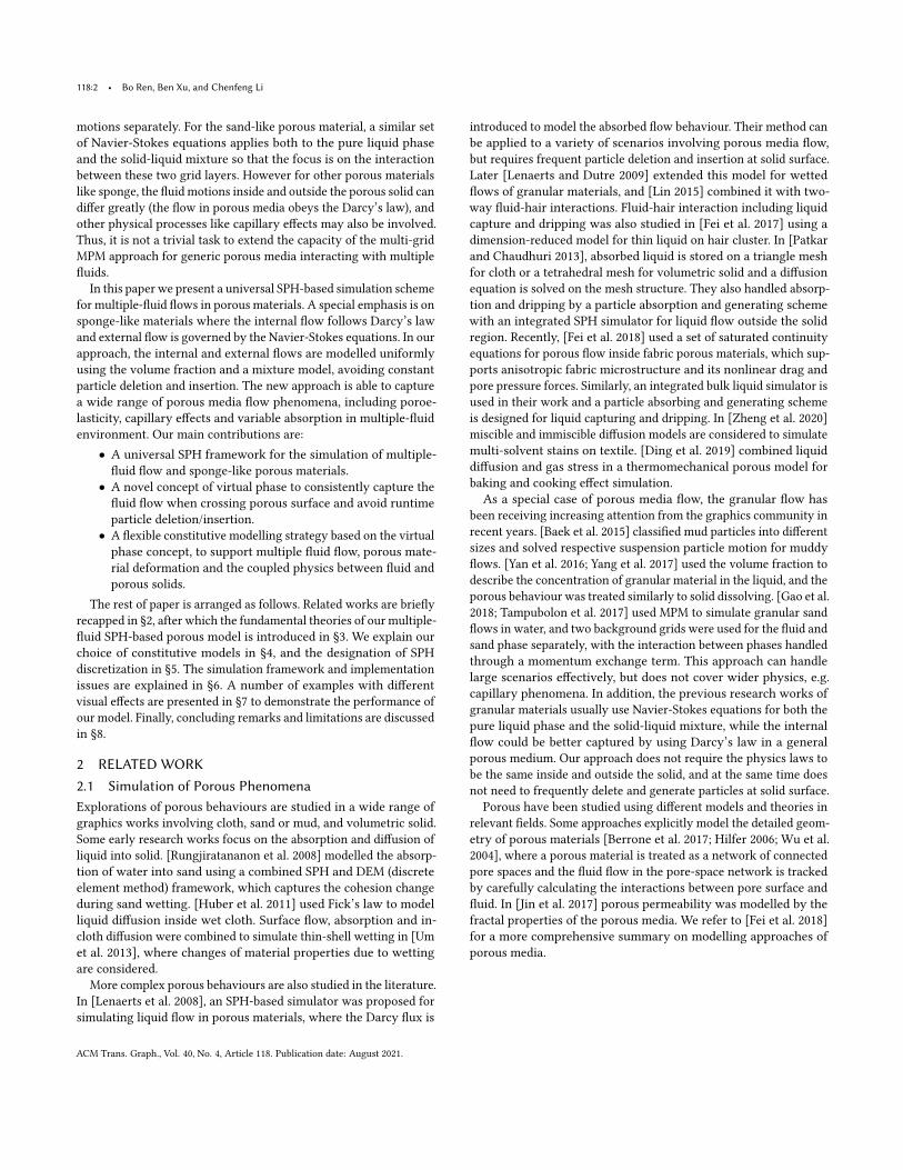
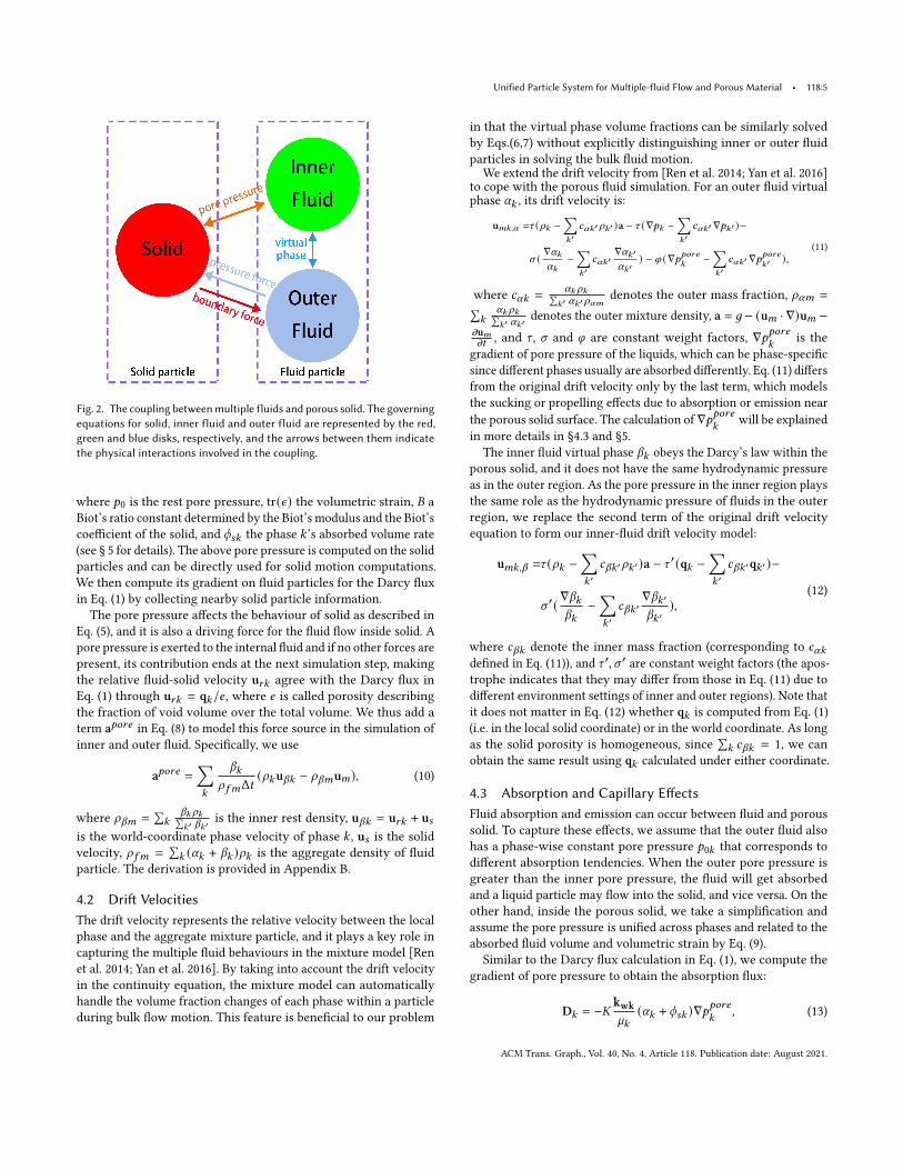
Fig. 3. Particle behavior on solid-liquid boundaries. (a) A two-phase liquid reaches the surface of a porous solid, the yellow phase is absorbable and the greenphase is non-absorbable. (b)(c)(d) The absorption flux first transfers the yellow phase to its virtual orange phase, which in turn is subject to the Darcy fluxtrying to drag the particle inside. Different drift velocities are produced among the virtual phases within a liquid particle. (e) The absorbed particles will be leftwith more absorbed phase as it goes deeper, and the non-absorbed-phase volume fractions are transferred to the outer-region particles.

where 𝐾 is a constant absorption ratio coefficient related to thesolid. The dimensionless term (𝛼𝑘 + 𝜙𝑠𝑘 ) is multiplied to avoidcreating fake flux. Then, Eq. (7) and Eq. (6) are used to determinethe exchange of internal and external fluids.When a part of fluid mass is absorbed by the solid, the fluid

particle will be subject to capillary force near the solid surface,preventing liquid escaping from the porous solid. We use a similarmodel as [Becker and Teschner 2007b] to capture the accelerationdue to capillary force:

a𝑐𝑎𝑝 = 𝜓∑𝑘

𝛽𝑘n, (14)

where 𝜓 is a constant strength factor, n is a normal vector in thedirection from a fluid particle to porous solid interior. Near theporous surface, the capillary force generates an inward draggingeffect. After the particle flows into the solid, it will gradually reduceto zero so that the motion of fluid particles gets purely governed bythe Darcy’s law.

4.4 Particle Behavior on Solid-liquid BoundariesIn this subsection we discuss how the coupling mechanisms in Fig. 2act on a fluid particle near the solid boundary in our simulationframework. In Fig. 3 we use a simple setting to demonstrate howphases within liquid particles change near the solid boundary whenthey are absorbed. In Fig. 3(a) a two-phase liquid with one phaseabsorbable (yellow) and one phase non-absorbable (green) reachesthe surface of a porous solid. In Fig. 3(b)(c)(d), the absorption flux(Eqn. (13)) will first act to transfer virtual phases (from yellow toorange). Then the inner virtual phase is subject to the Darcy flux,which is an inward-direction effect trying to drag the particle inside.At this time the particle will contain different velocities between

(virtual) phases, and they produce drift velocities. Roughly speaking,the absorbed phase will have a drift velocity pointing inward thesolid, the non-absorbed phase will have a drift velocity pointingoutward. The mixture model (Eqns. (6-8)) ensures that both con-centration change and particle motion change can be adequatelycalculated. As a result, in Fig. 3(e) the absorbed particles will be leftwith more absorbed phase as it goes deeper, and the non-absorbed-phase volume fractions are transferred to the outer-region particles(Eqns. (6-7)).

5 DISCRETIZATIONIn the SPH formulation, calculation of physical variables are per-formed through a weighted sum over neighbourhood particles. Ana-logue to the staggered-grid scheme, we find it convenient for somegradient and interpolation calculations to be selectively assignedto solid and fluid particles, since the solid particles can serve asreference background frame for the fluid particles nearby. Table 1lists the model variables with the storage particle categories theybelong to. In the following sections, we use

∑𝑠 for summing over

nearby solid particle quantities,∑

𝑓 for summing over nearby liquidparticle quantities, and

∑𝑘 for summing over 𝑘 phases. Subscript 𝑓

and 𝑠 indicate fluid and solid, respectively.The interpolated densities for the solid or fluid particles are com-

puted over the same kind of particles, i.e. for a particle 𝑖 , 𝜌𝑠,𝑖 =∑𝑗 𝑚𝑠,𝑗𝑊𝑖 𝑗 and 𝜌 𝑓 ,𝑖 =

∑𝑗 𝑚𝑓 , 𝑗𝑊𝑖 𝑗 .

The absorbed volume rate 𝜙𝑠𝑘 represents how much fluid phase𝑘 is absorbed locally at a solid particle position. It is calculated by

𝜙𝑠𝑘 =1

𝜌𝑘𝑉𝑠0

∑𝑓

𝛽𝑘𝑚𝑓 𝜌𝑘𝑊𝑓 𝑠

𝜌 𝑓𝑚𝑁𝑓

, (15)



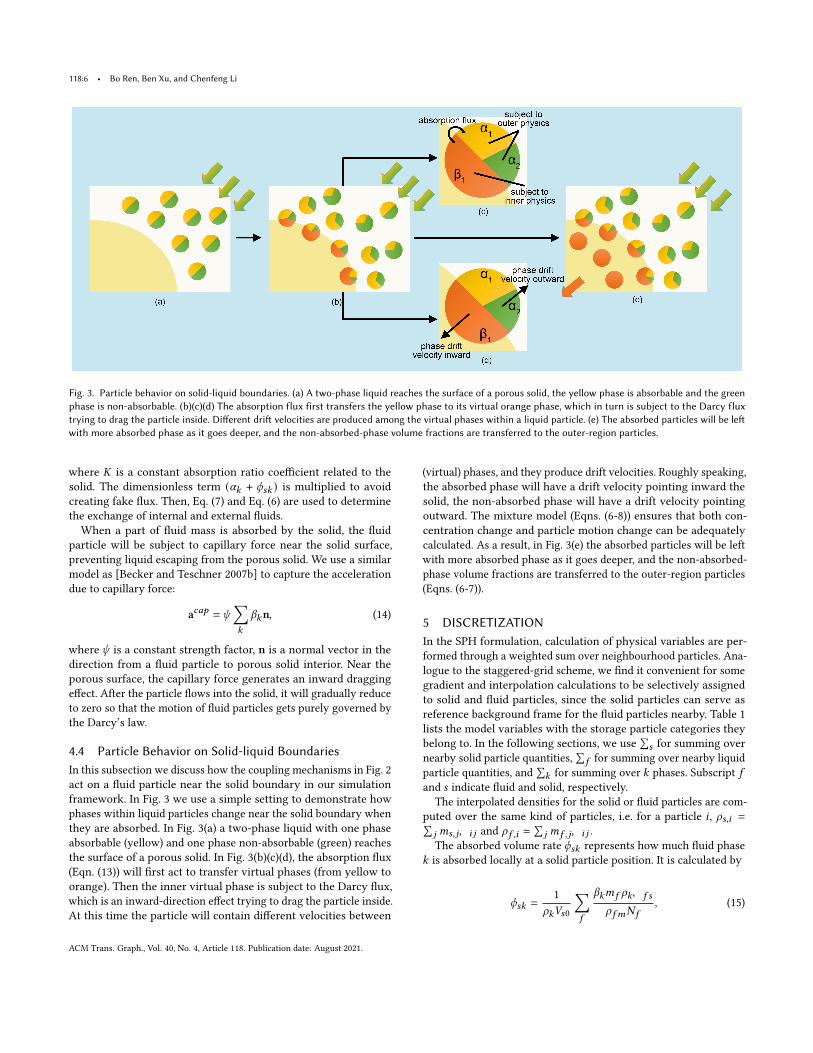
Table 1. Definition and Computation of Model Variables

Variable Description Storage/Calculation Location𝑚𝑠 ,𝑚𝑓 solid/fluid particle masses solid particle / fluid particle𝛼𝑘 , 𝛽𝑘 virtual phase volume fraction fluid particle

u𝑚𝑘,𝛼 , u𝑚𝑘,𝛽 drift velocities of virtual phases fluid particleu𝑚, u𝑠 fluid and solid particle velocities fluid particle / solid particleu𝑟𝑘 relative fluid-solid velocity of phase 𝑘 solid particleu𝛽𝑘 world-coordinate fluid phase velocity solid particle / fluid particle

u𝑚𝑘 , 𝛼𝑘 non-virtual drift velocity and volume fraction fluid particle𝜌 𝑓𝑚, 𝜌𝑘 fluid aggregate density and phase density fluid particle𝜌 𝑓 , 𝜌𝑠 , 𝜌𝑖 interpolated density of fluid/solid/particle 𝑖 fluid particle𝜌𝛼𝑚, 𝜌𝛽𝑚 outer/inner fluid mixture rest densities fluid particle𝑐𝛼𝑘 , 𝑐𝛽𝑘 outer/inner mass fractions fluid particle

q𝑘 Darcy flux of phase 𝑘 solid particle / fluid particle𝑝𝑝𝑜𝑟𝑒𝑠 pore pressure in solid solid particle𝑝0𝑘 fluid phase-wise pore pressure fluid particle

∇𝑝𝑝𝑜𝑟𝑒 ,∇𝑝𝑝𝑜𝑟𝑒𝑘

gradient of pore pressure (for phase 𝑘) solid particle / fluid particlea𝑝𝑟𝑒𝑠𝑠 , a𝑝𝑜𝑟𝑒 , a𝑐𝑎𝑝 , a𝑜𝑡ℎ𝑒𝑟 accelerations due to related forces fluid particle

𝜖 , P solid strain and stress tensors solid particleD𝑘 absorption flux fluid particle𝜙𝑠𝑘 absorbed volume rate solid particlen normal vector near solid surface fluid particle

𝑊, 𝑁𝑓 SPH kernel, sum of SPH kernels fluid particle

where 𝑉𝑠0 denotes the rest volume of solid particle, 𝜌𝑘 the restdensity of phase 𝑘 , 𝑁𝑓 =

∑𝑠𝑊𝑓 𝑠 the sum of SPH kernels between

each fluid particle and its nearby solid neighbours. For any fluidparticle with non-zero 𝛽𝑓 𝑘 , we effectively assign its absorbed massto nearby solid particles using an SPH-kernel weight, and Eq. (15)is the collected absorbed mass on a solid particle from nearby fluidparticle contributions. Detailed derivations are given in Appendix A.The model variables 𝑝𝑝𝑜𝑟𝑒𝑠 , q𝑘 , u𝑟𝑘 , u𝛽𝑘 are also computed on solidparticles. Then we are able to interpolate q𝑘 , u𝛽𝑘 onto fluid particlesusing the SPH formulation whenever needed:

u𝛽𝑘,𝑓 =∑𝑠

u𝛽𝑘,𝑠𝑊𝑓 𝑠/𝑁𝑓 (16)

q𝑘,𝑓 =∑𝑠

q𝑘,𝑠𝑊𝑓 𝑠/𝑁𝑓 . (17)

In the special case when 𝑁𝑓 = 0, we simply set the left hand side tobe zero.Using the SPH formulation, on a fluid particle Eq. (14) can be

discretized as:

a𝑐𝑎𝑝𝑓

= 𝜓∑𝑘

(𝛽𝑘∑𝑠

𝑚𝑠

𝜌𝑠∇𝑊𝑓 𝑠 ). (18)

There are several pore pressure gradients in Eqs.(1,11,13). InEq. (1), for each solid particle 𝑠 , the gradient of pore pressure iscomputed by:

∇𝑝𝑝𝑜𝑟𝑒𝑠 =∑

𝑠 𝑗 ∈𝑁𝑠

𝑚𝑠 𝑗

𝜌𝑠 𝑗(𝑝𝑝𝑜𝑟𝑒𝑠 − 𝑝𝑝𝑜𝑟𝑒𝑠 𝑗 )∇𝑊𝑠𝑠 𝑗 , (19)

where 𝑁𝑠 consists of the solid particles in 𝑠’s neighbourhood.

For fluid particles, in Eq. (11), the gradient of outer fluid porepressure is computed by

∇𝑝𝑝𝑜𝑟𝑒𝑓 𝑘

=∑𝑠

𝑚𝑠

𝜌𝑠(𝑝0𝑘 − 𝑝

𝑝𝑜𝑟𝑒𝑠 )∇𝑊𝑓 𝑠 , (20)

where 𝑝0𝑘 is defined in §4.3. For Eq. (13), we similarly have

D𝑘,𝑓 = −𝐾 kwk`𝑘

∑𝑠

𝑚𝑠

𝜌𝑠(𝛼 𝑓 𝑘 + 𝜙𝑠𝑘 ) (𝑝0𝑘 − 𝑝

𝑝𝑜𝑟𝑒𝑠 )∇𝑊𝑓 𝑠 . (21)

Then we compute the absorption source term using

∇ · D𝑘,𝑓 =∑𝑠

𝑚𝑠

𝜌𝑠D𝑘,𝑓 · ∇𝑊𝑓 𝑠 . (22)

6 IMPLEMENTATIONAlgorithm 1 summarizes the overall simulation workflow. The calcu-lation pipeline computes solid and fluid quantities in an interleavedmanner, and the calculation steps are performed on all fluid or solidparticles without labelling particle regions.

6.1 Outer Region Fluid HandlingInstead of using the state equation based approach as in [Ren et al.2014; Yan et al. 2016], we use an IISPH-like scheme to compute thehydrodynamic pressure for the outer-region fluid particles, whichgives better incompressibility. We adopt the same algorithm frame-work as [Band et al. 2018a] to compute pressure and implementtwo-way coupling. A series of modifications are made to supportmultiple-fluid porous flow simulation.



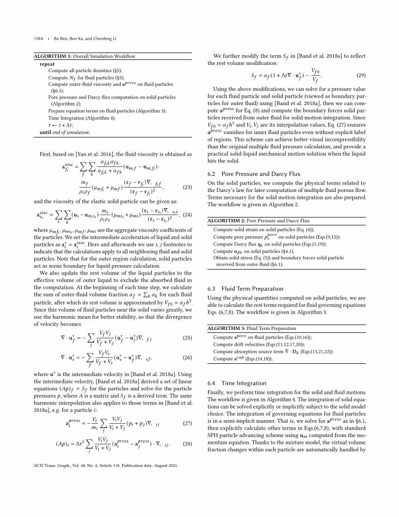
ALGORITHM 1: Overall Simulation Workflowrepeat

Compute all particle densities (§5);Compute 𝑁𝑓 for fluid particles (§5);Compute outer-fluid viscosity and a𝑝𝑟𝑒𝑠𝑠 on fluid particles(§6.1);

Pore pressure and Darcy flux computation on solid particles(Algorithm 2);

Prepare equation terms on fluid particles (Algorithm 3);Time Integration (Algorithm 4);𝑡 ← 𝑡 + Δ𝑡 ;

until end of simulation;

First, based on [Yan et al. 2016], the fluid viscosity is obtained as

a𝑣𝑖𝑠𝑐𝑓𝑖

=∑𝑓

∑𝑘

𝛼 𝑓𝑖𝑘𝛼 𝑓 𝑘

𝛼 𝑓𝑖𝑘 + 𝛼 𝑓 𝑘(u𝑚,𝑓 − u𝑚,𝑓𝑖 )·

𝑚𝑓

𝜌𝑖𝜌 𝑓(`𝑚𝑓𝑖 + `𝑚𝑓 )

(r𝑓 − r𝑓𝑖 )∇𝑊𝑓𝑖 𝑓

(r𝑓 − r𝑓𝑖 )2, (23)

and the viscosity of the elastic solid particle can be given as:

a𝑣𝑖𝑠𝑐𝑠𝑖=∑𝑠

∑𝑘

(u𝑠 −u𝑚,𝑠𝑖 )𝑚𝑠

𝜌𝑖𝜌𝑠(`𝑚𝑠𝑖 + `𝑚𝑠 )

(r𝑠 − r𝑠𝑖 )∇𝑊𝑠𝑖𝑠

(r𝑠 − r𝑠𝑖 )2, (24)

where `𝑚𝑓𝑖 , `𝑚𝑠𝑖 , `𝑚𝑓 , `𝑚𝑠 are the aggregate viscosity coefficients ofthe particles. We set the intermediate acceleration of liquid and solidparticles as a∗

𝑖= a𝑣𝑖𝑠𝑐

𝑖. Here and afterwards we use 𝑖, 𝑗 footnotes to

indicate that the calculations apply to all neighboring fluid and solidparticles. Note that for the outer region calculation, solid particlesact as scene boundary for liquid pressure calculation.We also update the rest volume of the liquid particles to the

effective volume of outer liquid to exclude the absorbed fluid inthe computation. At the beginning of each time step, we calculatethe sum of outer-fluid volume fraction 𝛼 𝑓 =

∑𝑘 𝛼𝑘 for each fluid

particle, after which its rest volume is approximated by 𝑉𝑓 0 = 𝛼 𝑓 ℎ3.Since this volume of fluid particles near the solid varies greatly, weuse the harmonic mean for better stability, so that the divergenceof velocity becomes

∇ · u∗𝑓= −

∑𝑗

𝑉𝑓𝑉𝑗

𝑉𝑓 +𝑉𝑗(u∗

𝑓− u∗𝑗 )∇𝑊𝑓 𝑗 (25)

∇ · u∗𝑠 = −∑𝑓

𝑉𝑓𝑉𝑠

𝑉𝑓 +𝑉𝑠(u∗𝑠 − u∗𝑓 )∇𝑊𝑠 𝑓 , (26)

where u∗ is the intermediate velocity in [Band et al. 2018a]. Usingthe intermediate velocity, [Band et al. 2018a] derived a set of linearequations (𝐴𝑝)𝑓 = 𝑆𝑓 for the particles and solve for the particlepressures 𝑝 , where 𝐴 is a matrix and 𝑆𝑓 is a derived term. The sameharmonic interpolation also applies to those terms in [Band et al.2018a], e.g. for a particle 𝑖:

a𝑝𝑟𝑒𝑠𝑠𝑖

= − 𝑉𝑖𝑚𝑖

∑𝑗

𝑉𝑖𝑉𝑗

𝑉𝑖 +𝑉𝑗(𝑝𝑖 + 𝑝 𝑗 )∇𝑊𝑖 𝑗 (27)

(𝐴𝑝)𝑖 = Δ𝑡2∑𝑗

𝑉𝑖𝑉𝑗

𝑉𝑖 +𝑉𝑗(a𝑝𝑟𝑒𝑠𝑠

𝑖− a𝑝𝑟𝑒𝑠𝑠

𝑗) · ∇𝑊𝑖 𝑗 . (28)

We further modify the term 𝑆𝑓 in [Band et al. 2018a] to reflectthe rest volume modification:

𝑆𝑓 = 𝛼 𝑓 (1 + Δ𝑡∇ · u∗𝑓 ) −𝑉𝑓 0

𝑉𝑓. (29)

Using the above modifications, we can solve for a pressure valuefor each fluid particle and solid particle (viewed as boundary par-ticles for outer fluid) using [Band et al. 2018a], then we can com-pute a𝑝𝑟𝑒𝑠𝑠 for Eq. (8) and compute the boundary forces solid par-ticles received from outer fluid for solid motion integration. Since𝑉𝑓 0 = 𝛼 𝑓 ℎ

3 and 𝑉𝑖 ,𝑉𝑗 are its interpolation values, Eq. (27) ensuresa𝑝𝑟𝑒𝑠𝑠 vanishes for inner fluid particles even without explicit labelof regions. This scheme can achieve better visual incompressibilitythan the original multiple fluid pressure calculation, and provide apractical solid-liquid mechanical motion solution when the liquidhits the solid.

6.2 Pore Pressure and Darcy FluxOn the solid particles, we compute the physical terms related tothe Darcy’s law for later computation of multiple fluid porous flow.Terms necessary for the solid motion integration are also prepared.The workflow is given in Algorithm 2.

ALGORITHM 2: Pore Pressure and Darcy Flux

Compute solid strain on solid particles (Eq. (4));Compute pore pressure 𝑝𝑝𝑜𝑟𝑒𝑠 on solid particles (Eqs.(9,15));Compute Darcy flux q𝑘 on solid particles (Eqs.(1,19));Compute u𝛽𝑘 on solid particles (§4.1);Obtain solid stress (Eq. (5)) and boundary forces solid particlereceived from outer fluid (§6.1);

6.3 Fluid Term PreparationUsing the physical quantities computed on solid particles, we areable to calculate the rest terms required for fluid governing equationsEqs. (6,7,8). The workflow is given in Algorithm 3.

ALGORITHM 3: Fluid Term Preparation

Compute a𝑝𝑜𝑟𝑒 on fluid particles (Eqs.(10,16));Compute drift velocities (Eqs.(11,12,17,20));Compute absorption source term ∇ · D𝑘 (Eqs.(13,21,22));Compute a𝑐𝑎𝑝 (Eqs.(14,18));

6.4 Time IntegrationFinally, we perform time integration for the solid and fluid motions.The workflow is given in Algorithm 4. The integration of solid equa-tions can be solved explicitly or implicitly subject to the solid modelchoice. The integration of governing equations for fluid particlesis in a semi-implicit manner. That is, we solve for a𝑝𝑟𝑒𝑠𝑠 as in §6.1,then explicitly calculate other terms in Eqs.(6,7,8), with standardSPH particle advancing scheme using u𝑚 computed from the mo-mentum equation. Thanks to the mixture model, the virtual volumefraction changes within each particle are automatically handled by



integration of the continuity equations, where the volume fractionchanges rely on local divergences, and no explicit mass or volumefraction advection is needed. However, the explicit integration isstill subject to CFL conditions that limits the time step size, a de-tailed discussion can be found in [Ren et al. 2014]. It is noted thatalthough we adopt [Peer et al. 2018] for the solid model by default,our algorithm framework has the flexibility to allow for other kindsof solid physical models. An example is given in §7 Fig. 11, where weuse the solid model in [Yang et al. 2017] and simulates a two-phasesand-water flow. We ensure

∑𝑘 (𝛼𝑘 + 𝛽𝑘 ) = 1 in a similar way with

[Ren et al. 2014], i.e. first setting negative values of 𝛼𝑘 , 𝛽𝑘 to zero,and then re-scale them so that their sum equals 1.

ALGORITHM 4: Time Integration

Integrate solid particle motion using [Peer et al. 2018];Integrate Eqs.(6,7,8);for each fluid particle do

Ensure∑

𝑘 (𝛼𝑘 + 𝛽𝑘 ) = 1 (§6.4);if (𝑁𝑓 == 0) then

𝛼𝑘+ = 𝛽𝑘 ;𝛽𝑘 = 0;

endend

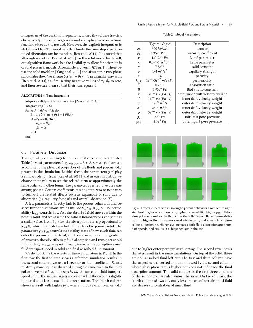
6.5 Parameter DiscussionThe typical model settings for our simulation examples are listedTable 2. Most parameters (e.g. 𝜌𝑘 , `𝑘 , a, _, [, 𝐵, 𝜏, 𝜎, 𝜎 ′,𝜓, 𝑒) are setaccording to the physical properties of the fluids and porous solidpresent in the simulation. Besides these, the parameters 𝜑, 𝜏 ′ playa similar role to 𝜏 from [Ren et al. 2014], and in our simulation wechoose their values to set the related term at approximately thesame order with other terms. The parameter `𝑘 is set to be the sameamong phases. Certain coefficients can be set to zero or near-zeroto turn-off the related effects such as expansion of solid due toabsorption ([), capillary force (𝜓 ) and overall absorption (𝐾 ).A few parameters directly link to the porous behaviour and de-

serve further discussions, which include 𝑝0, 𝑝0𝑘 , k𝑤𝑘 , 𝐾 . The perme-ability k𝑤𝑘 controls how fast the absorbed fluid moves within theporous solid, and we assume the solid is homogeneous and set it asa scalar value. From Eq. (13), the absorption rate is proportional tok𝑤𝑘𝐾 , which controls how fast fluid enters the porous solid. Theparameters 𝑝0, 𝑝0𝑘 controls the stability state of how much fluid canenter the porous solid in total, and they also influence the gradientof pressure, thereby affecting fluid absorption and transport speedin solid. Higher 𝑝0𝑘 − 𝑝0 will usually increase the absorption speed,fluid transport speed in solid and final absorbed fluid amount.We demonstrate the effects of these parameters in Fig. 4. In the

first row, the first column shows a reference simulation results. Inthe second column, we use a larger absorption coefficient 𝐾 , andrelatively more liquid is absorbed during the same time. In the thirdcolumn, we raise 𝑘𝑤𝑘 but keeps 𝑘𝑤𝑘𝐾 the same, the fluid transportspeed within the solid is largely increased while the colour is slightlylighter due to less dense fluid concentration. The fourth columnshows a result with higher 𝑝0𝑘 , where fluid is easier to enter solid

Table 2. Model Parameters

Typical Value Description𝜌𝑘 600 𝑘𝑔/𝑚3 density`𝑘 0.35-1 𝑃𝑎 · 𝑠 viscosity coefficienta 1𝑒4-2𝑒4 𝑃𝑎 Lamé parameter_ 0.5𝑒4-1.2𝑒4 𝑃𝑎 Lamé parameter[ 7.5𝑒−4 solid constant𝜓 1-4𝑚2/𝑠2 capillary strength𝑒 0.6 porosity𝑘𝑤𝑘 1𝑒−8-5𝑒−7 𝑚2𝑠/𝑃𝑎 permeability𝐾 0.75-2 absorption ratio𝐵 4.90𝑒4 𝑃𝑎 Biot’s ratio constant𝜏 3𝑒−6 𝑚/(𝑃𝑎 · 𝑠) outer/inner drift velocity weight𝜏 ′ 1𝑒−4 𝑚/(𝑃𝑎 · 𝑠) inner drift velocity weight𝜎 1𝑒−3 𝑚2/𝑠 outer drift velocity weight𝜎 ′ 2𝑒−3 𝑚2/𝑠 inner drift velocity weight𝜑 3𝑒−6 𝑚/(𝑃𝑎 · 𝑠) outer drift velocity weight𝑝0 5𝑒4 𝑃𝑎 solid rest pore pressure𝑝0𝑘 2.5𝑒4 𝑃𝑎 outer liquid pore pressure

Fig. 4. Effects of parameters linking to porous behaviors. From left to right:standard, higher absorption rate, higher permeability, higher 𝑝0𝑘 . Higherabsorption rate makes the fluid enter the solid faster. Higher permeabilityleads to higher fluid transport speed within solid, and results in a lightercolour at beginning. Higher 𝑝0𝑘 increases both fluid absorption and trans-port speeds, and results in a deeper colour in the end.

due to higher outer pore pressure setting. The second row showsthe later result in the same simulations. On top of the solid, thereare non-absorbed fluid left out. The first and third column havethe largest non-absorbed amount followed by the second column,whose absorption rate is higher but does not influence the finalabsorption amount. The solid colours in the first three columnsof the second row are also almost the same. On the contrary, thefourth column shows obviously less amount of non-absorbed fluidand denser concentration of inner fluid.



Table 3. Performance Data

Liquid Liquid Solid runtimePhases Particles Particles (second/step)

Example 1 1 402,000 247,000 0.36Example 2 2 980,000 120,000 0.47Example 3 1 1,683,000 41,000 0.40Example 4 2 1,091,000 524,000 0.42Example 5 3 693,000 448,000 0.38Example 6 3 1,055,000 2,098,000 0.84Example 7 1 178,000 133,000 0.09

7 RESULTSWe implemented the proposed approach on an Nvidia GeForce GTX1080Ti GPU. The performances of the simulations in this section arerecorded in Table 3. In the experiments, the particle mass and thewidth of the scene are typically set to 0.2𝑔 and between 0.1𝑚 − 1𝑚.We generally choose a fixed time step that is below the CFL timesteps and ensures the solid solver and outer-fluid solver are bothstable. Each frame in the supplemental video (30 frames per second)contains 10 steps.

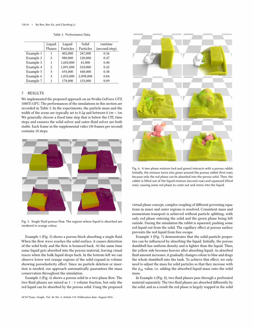
Fig. 5. Single fluid porous flow. The regions where liquid is absorbed arerendered in orange colour.

Example 1 (Fig. 5) shows a porous block absorbing a single fluid.When the flow wave reaches the solid surface, it causes distortionof the solid body and the flow is bounced back. At the same timesome liquid gets absorbed into the porous material, leaving visualtraces when the bulk liquid drops back. In the bottom-left we canobserve lower wet orange regions of the solid expand in volumeshowing poroelasticity effect. Since no particle deletion or inser-tion is needed, our approach automatically guarantees the massconservation throughout the simulation.

Example 2 (Fig. 6) shows a porous solid in a two-phase flow. Thetwo fluid phases are mixed as 1 : 1 volume fraction, but only thered liquid can be absorbed by the porous solid. Using the proposed

Fig. 6. A two-phase mixture (red and green) interacts with a porous rabbit.Initially, the mixture turns into green around the porous rabbit (first row),because only the red phase can be absorbed into the porous solid. Then, therabbit is lifted out of the liquid mixture (second row) and squeezed (thirdrow), causing some red phase to come out and remix into the liquid.

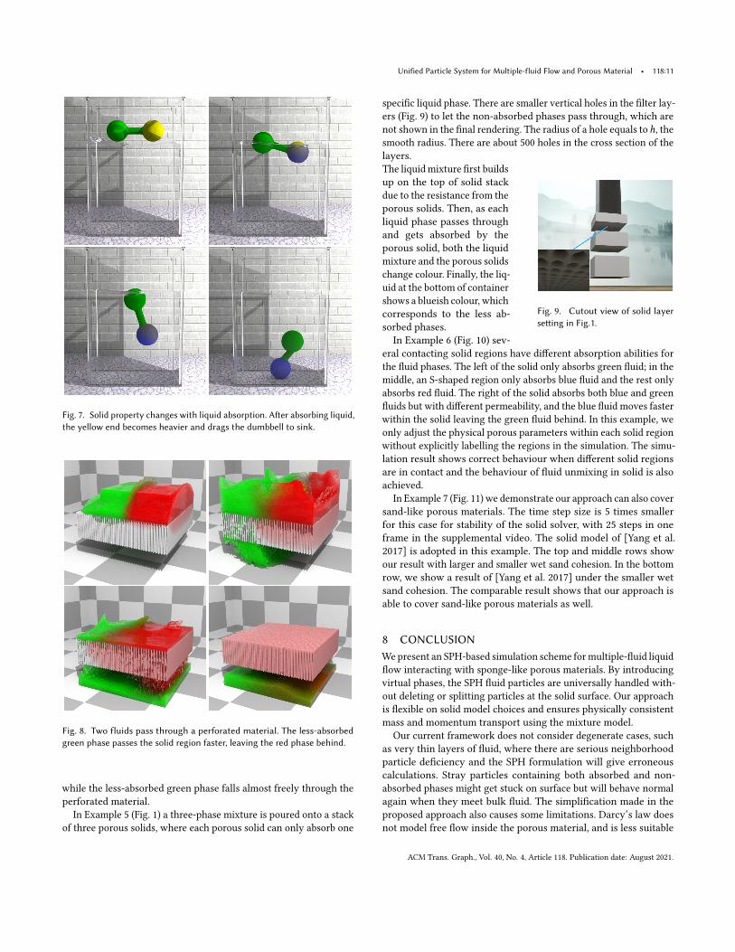
virtual phase concept, complex coupling of different governing equa-tions in inner and outer regions is resolved. Consistent mass andmomentum transport is achieved without particle splitting, withonly red phase entering the solid and the green phase being leftoutside. During the simulation the rabbit is squeezed, pushing somered liquid out from the solid. The capillary effect at porous surfaceprevents the red liquid from free escape.Example 3 (Fig. 7) demonstrates that the solid-particle proper-

ties can be influenced by absorbing the liquid. Initially, the porousdumbbell has uniform density and is lighter than the liquid. Then,the yellow side becomes heavier after absorbing liquid. As absorbedfluid amount increases, it gradually changes colour to blue and dragsthe whole dumbbell into the tank. To achieve this effect, we onlyneed to adjust the mass for solid particles so that they increase withthe 𝜙𝑠𝑘 value, i.e. adding the absorbed liquid mass onto the solidmass.

In Example 4 (Fig. 8), two fluid phases pass through a perforatedmaterial separately. The two fluid phases are absorbed differently bythe solid, and as a result the red phase is largely trapped in the solid



Fig. 7. Solid property changes with liquid absorption. After absorbing liquid,the yellow end becomes heavier and drags the dumbbell to sink.

Fig. 8. Two fluids pass through a perforated material. The less-absorbedgreen phase passes the solid region faster, leaving the red phase behind.

while the less-absorbed green phase falls almost freely through theperforated material.

In Example 5 (Fig. 1) a three-phase mixture is poured onto a stackof three porous solids, where each porous solid can only absorb one

specific liquid phase. There are smaller vertical holes in the filter lay-ers (Fig. 9) to let the non-absorbed phases pass through, which arenot shown in the final rendering. The radius of a hole equals toℎ, thesmooth radius. There are about 500 holes in the cross section of thelayers.

Fig. 9. Cutout view of solid layersetting in Fig.1.

The liquidmixture first buildsup on the top of solid stackdue to the resistance from theporous solids. Then, as eachliquid phase passes throughand gets absorbed by theporous solid, both the liquidmixture and the porous solidschange colour. Finally, the liq-uid at the bottom of containershows a blueish colour, whichcorresponds to the less ab-sorbed phases.In Example 6 (Fig. 10) sev-

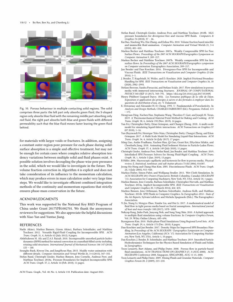
eral contacting solid regions have different absorption abilities forthe fluid phases. The left of the solid only absorbs green fluid; in themiddle, an S-shaped region only absorbs blue fluid and the rest onlyabsorbs red fluid. The right of the solid absorbs both blue and greenfluids but with different permeability, and the blue fluid moves fasterwithin the solid leaving the green fluid behind. In this example, weonly adjust the physical porous parameters within each solid regionwithout explicitly labelling the regions in the simulation. The simu-lation result shows correct behaviour when different solid regionsare in contact and the behaviour of fluid unmixing in solid is alsoachieved.

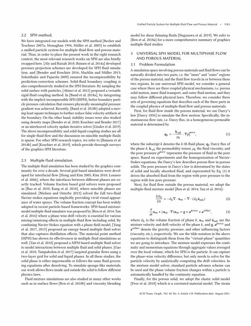
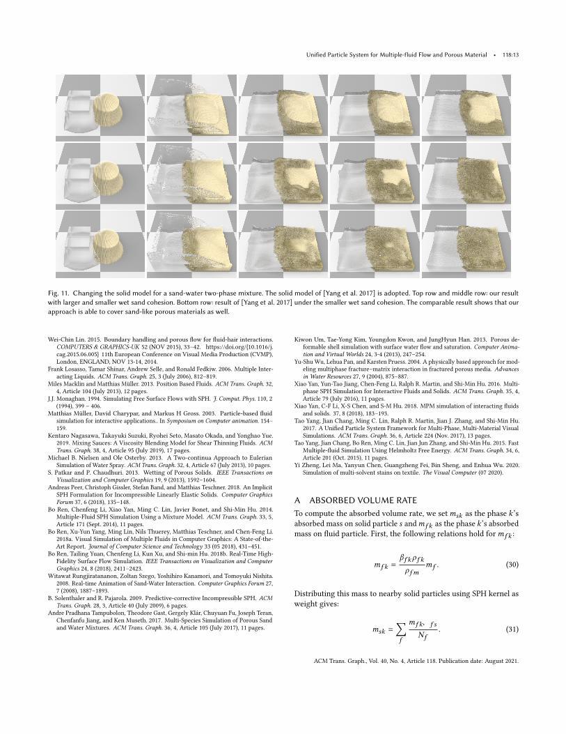
In Example 7 (Fig. 11) we demonstrate our approach can also coversand-like porous materials. The time step size is 5 times smallerfor this case for stability of the solid solver, with 25 steps in oneframe in the supplemental video. The solid model of [Yang et al.2017] is adopted in this example. The top and middle rows showour result with larger and smaller wet sand cohesion. In the bottomrow, we show a result of [Yang et al. 2017] under the smaller wetsand cohesion. The comparable result shows that our approach isable to cover sand-like porous materials as well.

8 CONCLUSIONWepresent an SPH-based simulation scheme formultiple-fluid liquidflow interacting with sponge-like porous materials. By introducingvirtual phases, the SPH fluid particles are universally handled with-out deleting or splitting particles at the solid surface. Our approachis flexible on solid model choices and ensures physically consistentmass and momentum transport using the mixture model.

Our current framework does not consider degenerate cases, suchas very thin layers of fluid, where there are serious neighborhoodparticle deficiency and the SPH formulation will give erroneouscalculations. Stray particles containing both absorbed and non-absorbed phases might get stuck on surface but will behave normalagain when they meet bulk fluid. The simplification made in theproposed approach also causes some limitations. Darcy’s law doesnot model free flow inside the porous material, and is less suitable



Fig. 10. Porous behaviour in multiple contacting solid regions. The solidcomprises three parts: the left part only absorbs green fluid, the S-shapedregion only absorbs blue fluid with the remainingmiddle part absorbing onlyred fluid, the right part absorbs both blue and green fluids with differentpermeability such that the blue fluid moves faster leaving the green fluidbehind.

for materials with larger voids or fractures. In addition, assigninga constant outer-region pore pressure for each phase during solid-surface absorption is a simple and effective treatment, but may notbe enough for certain cases where complex relative absorption ten-dency variations between multiple solid and fluid phases exist. Apossible solution involves decoupling the phase-wise pore pressuresin the solid, which we would like to investigate in the future. Thevolume fraction correction in Algorithm 4 is explicit and does nottake consideration of its influence to the momentum calculation,which may produce errors in mass calculation under very large timesteps. We would like to investigate efficient combined integrationmethods of the continuity and momentum equations that strictlyensures phase-mass conservation in the future.

ACKNOWLEDGMENTSThis work was supported by the National Key R&D Program ofChina under Grant 2017YFB1002701. We thank the anonymousreviewers for suggestions.We also appreciate the helpful discussionswith Xiao Yan and Yuntao Jiang.

REFERENCESNadir Akinci, Markus Ihmsen, Gizem Akinci, Barbara Solenthaler, and Matthias

Teschner. 2012. Versatile Rigid-Fluid Coupling for Incompressible SPH. ACMTrans. Graph. 31, 4, Article 62 (July 2012), 8 pages.

Abdelraheem M. Aly and Z.A.S. Raizah. 2018. Incompressible smoothed particle hydro-dynamics (ISPH) method for natural convection in a nanofluid-filled cavity includingrotating solid structures. International Journal of Mechanical Sciences 146-147 (2018),125 – 140.

Seungho Baek, Kiwon Um, and JungHyun Han. 2015. Muddy water animation withdifferent details. Computer Animation and Virtual Worlds 26, 3-4 (2015), 347–355.

Stefan Band, Christoph Gissler, Markus Ihmsen, Jens Cornelis, Andreas Peer, andMatthias Teschner. 2018a. Pressure Boundaries for Implicit Incompressible SPH.ACM Trans. Graph. 37, 2, Article 14 (Feb. 2018), 11 pages.

Stefan Band, Christoph Gissler, Andreas Peer, and Matthias Teschner. 2018b. MLSpressure boundaries for divergence-free and viscous SPH fluids. Computers &Graphics 76 (2018), 37 – 46.

Kai Bao, XiaolongWu, Hui Zhang, and EnhuaWu. 2010. Volume fraction based miscibleand immiscible fluid animation. Computer Animation and Virtual Worlds 21, 3-4(2010), 401–410.

Markus Becker and Matthias Teschner. 2007a. Weakly Compressible SPH for FreeSurface Flows. Proceedings of the 2007 ACM SIGGRAPH/Eurographics Symposium onComputer Animation 9, 209–217.

Markus Becker and Matthias Teschner. 2007b. Weakly compressible SPH for freesurface flows. In Proceedings of the 2007 ACM SIGGRAPH/Eurographics symposiumon Computer animation. Eurographics Association, 209–217.

Jan Bender and Dan Koschier. 2016. Divergence-Free SPH for Incompressible andViscous Fluids. IEEE Transactions on Visualization and Computer Graphics 23 (062016), 1–1.

J. Bender, T. Kugelstadt, M. Weiler, and D. Koschier. 2020. Implicit Frictional BoundaryHandling for SPH. IEEE Transactions on Visualization and Computer Graphics 26, 10(2020), 2982–2993.

Stefano Berrone, Sandra Pieraccini, and Stefano Scialo. 2017. Flow simulations in porousmedia with immersed intersecting fractures. JOURNAL OF COMPUTATIONALPHYSICS 345 (SEP 15 2017), 768–791. https://doi.org/10.1016/j.jcp.2017.05.049

Henry Philibert Gaspard Darcy. 1856. Les Fontaines publiques de la ville de Dijon.Exposition et application des principes à suivre et des formules à employer dans lesquestions de distribution d’eau, etc. V. Dalamont.

E. Detournay and Alexander H.-D. Cheng. 1993. 5 - Fundamentals of Poroelasticity. InAnalysis and Design Methods, CHARLES FAIRHURST (Ed.). Pergamon, Oxford, 113– 171.

Mengyuan Ding, Xuchen Han, Stephanie Wang, Theodore F. Gast, and Joseph M. Teran.2019. A Thermomechanical Material Point Method for Baking and Cooking. ACMTrans. Graph. 38, 6, Article 192 (Nov. 2019), 14 pages.

Yun Fei, Christopher Batty, Eitan Grinspun, and Changxi Zheng. 2018. A multi-scalemodel for simulating liquid-fabric interactions. ACM Transactions on Graphics 37(07 2018), 1–16.

Yun (Raymond) Fei, Henrique Teles Maia, Christopher Batty, Changxi Zheng, and EitanGrinspun. 2017. A Multi-Scale Model for Simulating Liquid-Hair Interactions. ACMTrans. Graph. 36, 4, Article 56 (July 2017), 17 pages.

Ming Gao, Andre Pradhana, Xuchen Han, Qi Guo, Grant Kot, Eftychios Sifakis, andChenfanfu Jiang. 2018. Animating Fluid Sediment Mixture in Particle-Laden Flows.ACM Trans. Graph. 37, 4, Article 149 (July 2018), 11 pages.

Christoph Gissler, Andreas Peer, Stefan Band, Jan Bender, and Matthias Teschner. 2019.Interlinked SPH Pressure Solvers for Strong Fluid-Rigid Coupling. ACM Trans.Graph. 38, 1, Article 5 (Jan. 2019), 13 pages.

R Hilfer. 2006. Macroscopic capillarity and hysteresis for flow in porous media. Physicalreview. E, Statistical, nonlinear, and soft matter physics 73 (02 2006), 016307.

Jeong-Mo Hong and Chang-Hun Kim. 2005. Discontinuous Fluids. ACM Trans. Graph.24, 3 (July 2005), 915–920.

Markus Huber, Simon Pabst, and Wolfgang Straßer. 2011. Wet Cloth Simulation. InACM SIGGRAPH 2011 Posters (Vancouver, British Columbia, Canada) (SIGGRAPH’11). Association for Computing Machinery, New York, NY, USA, Article 10, 1 pages.

Markus Ihmsen, Jens Cornelis, Barbara Solenthaler, Christopher Horvath, and MatthiasTeschner. 2014a. Implicit Incompressible SPH. IEEE Transactions on Visualizationand Computer Graphics 20, 3 (March 2014), 426–435.

Markus Ihmsen, Jens Orthmann, Barbara Solenthaler, Andreas Kolb, and MatthiasTeschner. 2014b. SPH Fluids in Computer Graphics. In Eurographics 2014 - State ofthe Art Reports, Sylvain Lefebvre and Michela Spagnuolo (Eds.). The EurographicsAssociation.

Yi Jin, Xiang Li, Mengyu Zhao, Xianhe Liu, and Hui Li. 2017. A mathematical model offluid flow in tight porous media based on fractal assumptions. International journalof heat and mass transfer 108 (2017), 1078–1088.

Nahyup Kang, Jinho Park, Junyong Noh, and Sung Yong Shin. 2010. A hybrid approachto multiple fluid simulation using volume fractions. In Computer Graphics Forum,Vol. 29. Wiley Online Library, 685–694.

Byungmoon Kim. 2010. Multi-phase Fluid Simulations Using Regional Level Sets. ACMTrans. Graph. 29, 6, Article 175 (Dec. 2010), 8 pages.

Dan Koschier and Jan Bender. 2017. Density Maps for Improved SPH Boundary Han-dling. In Proceedings of the ACM SIGGRAPH / Eurographics Symposium on ComputerAnimation (Los Angeles, California) (SCA ’17). Association for Computing Machin-ery, New York, NY, USA, Article 1, 10 pages.

Dan Koschier, J. Bender, B. Solenthaler, and Matthias Teschner. 2019. Smoothed ParticleHydrodynamics Techniques for the Physics Based Simulation of Fluids and Solids.In Eurographics.

Toon Lenaerts, Bart Adams, and Philip Dutre. 2008. Porous flow in particle-basedfluid simulations. ACM TRANSACTIONS ON GRAPHICS 27, 3 (AUG 2008). ACMSIGGRAPH Conference 2008, Singapore, SINGAPORE, AUG 11-15, 2008.

Toon Lenaerts and Philip Dutre. 2009. Mixing Fluids and Granular Materials. ComputerGraphics Forum 28, 2 (2009), 213–218.


https://doi.org/10.1016/j.jcp.2017.05.049


Fig. 11. Changing the solid model for a sand-water two-phase mixture. The solid model of [Yang et al. 2017] is adopted. Top row and middle row: our resultwith larger and smaller wet sand cohesion. Bottom row: result of [Yang et al. 2017] under the smaller wet sand cohesion. The comparable result shows that ourapproach is able to cover sand-like porous materials as well.

Wei-Chin Lin. 2015. Boundary handling and porous flow for fluid-hair interactions.COMPUTERS & GRAPHICS-UK 52 (NOV 2015), 33–42. https://doi.org/10.1016/j.cag.2015.06.005 11th European Conference on Visual Media Production (CVMP),London, ENGLAND, NOV 13-14, 2014.

Frank Losasso, Tamar Shinar, Andrew Selle, and Ronald Fedkiw. 2006. Multiple Inter-acting Liquids. ACM Trans. Graph. 25, 3 (July 2006), 812–819.

Miles Macklin and Matthias Müller. 2013. Position Based Fluids. ACM Trans. Graph. 32,4, Article 104 (July 2013), 12 pages.

J.J. Monaghan. 1994. Simulating Free Surface Flows with SPH. J. Comput. Phys. 110, 2(1994), 399 – 406.

Matthias Müller, David Charypar, and Markus H Gross. 2003. Particle-based fluidsimulation for interactive applications.. In Symposium on Computer animation. 154–159.

Kentaro Nagasawa, Takayuki Suzuki, Ryohei Seto, Masato Okada, and Yonghao Yue.2019. Mixing Sauces: A Viscosity Blending Model for Shear Thinning Fluids. ACMTrans. Graph. 38, 4, Article 95 (July 2019), 17 pages.

Michael B. Nielsen and Ole Osterby. 2013. A Two-continua Approach to EulerianSimulation of Water Spray. ACM Trans. Graph. 32, 4, Article 67 (July 2013), 10 pages.

S. Patkar and P. Chaudhuri. 2013. Wetting of Porous Solids. IEEE Transactions onVisualization and Computer Graphics 19, 9 (2013), 1592–1604.

Andreas Peer, Christoph Gissler, Stefan Band, and Matthias Teschner. 2018. An ImplicitSPH Formulation for Incompressible Linearly Elastic Solids. Computer GraphicsForum 37, 6 (2018), 135–148.

Bo Ren, Chenfeng Li, Xiao Yan, Ming C. Lin, Javier Bonet, and Shi-Min Hu. 2014.Multiple-Fluid SPH Simulation Using a Mixture Model. ACM Trans. Graph. 33, 5,Article 171 (Sept. 2014), 11 pages.

Bo Ren, Xu-Yun Yang, Ming Lin, Nils Thuerey, Matthias Teschner, and Chen-Feng Li.2018a. Visual Simulation of Multiple Fluids in Computer Graphics: A State-of-the-Art Report. Journal of Computer Science and Technology 33 (05 2018), 431–451.

Bo Ren, Tailing Yuan, Chenfeng Li, Kun Xu, and Shi-min Hu. 2018b. Real-Time High-Fidelity Surface Flow Simulation. IEEE Transactions on Visualization and ComputerGraphics 24, 8 (2018), 2411–2423.

Witawat Rungjiratananon, Zoltan Szego, Yoshihiro Kanamori, and Tomoyuki Nishita.2008. Real-time Animation of Sand-Water Interaction. Computer Graphics Forum 27,7 (2008), 1887–1893.

B. Solenthaler and R. Pajarola. 2009. Predictive-corrective Incompressible SPH. ACMTrans. Graph. 28, 3, Article 40 (July 2009), 6 pages.

Andre Pradhana Tampubolon, Theodore Gast, Gergely Klár, Chuyuan Fu, Joseph Teran,Chenfanfu Jiang, and Ken Museth. 2017. Multi-Species Simulation of Porous Sandand Water Mixtures. ACM Trans. Graph. 36, 4, Article 105 (July 2017), 11 pages.

Kiwon Um, Tae-Yong Kim, Youngdon Kwon, and JungHyun Han. 2013. Porous de-formable shell simulation with surface water flow and saturation. Computer Anima-tion and Virtual Worlds 24, 3-4 (2013), 247–254.

Yu-ShuWu, Lehua Pan, and Karsten Pruess. 2004. A physically based approach for mod-eling multiphase fracture–matrix interaction in fractured porous media. Advancesin Water Resources 27, 9 (2004), 875–887.

Xiao Yan, Yun-Tao Jiang, Chen-Feng Li, Ralph R. Martin, and Shi-Min Hu. 2016. Multi-phase SPH Simulation for Interactive Fluids and Solids. ACM Trans. Graph. 35, 4,Article 79 (July 2016), 11 pages.

Xiao Yan, C-F Li, X-S Chen, and S-M Hu. 2018. MPM simulation of interacting fluidsand solids. 37, 8 (2018), 183–193.

Tao Yang, Jian Chang, Ming C. Lin, Ralph R. Martin, Jian J. Zhang, and Shi-Min Hu.2017. A Unified Particle System Framework for Multi-Phase, Multi-Material VisualSimulations. ACM Trans. Graph. 36, 6, Article 224 (Nov. 2017), 13 pages.

Tao Yang, Jian Chang, Bo Ren, Ming C. Lin, Jian Jun Zhang, and Shi-Min Hu. 2015. FastMultiple-fluid Simulation Using Helmholtz Free Energy. ACM Trans. Graph. 34, 6,Article 201 (Oct. 2015), 11 pages.

Yi Zheng, Lei Ma, Yanyun Chen, Guangzheng Fei, Bin Sheng, and Enhua Wu. 2020.Simulation of multi-solvent stains on textile. The Visual Computer (07 2020).

A ABSORBED VOLUME RATETo compute the absorbed volume rate, we set𝑚𝑠𝑘 as the phase 𝑘’sabsorbed mass on solid particle 𝑠 and𝑚𝑓 𝑘 as the phase 𝑘’s absorbedmass on fluid particle. First, the following relations hold for𝑚𝑓 𝑘 :

𝑚𝑓 𝑘 =𝛽𝑓 𝑘𝜌 𝑓 𝑘

𝜌 𝑓𝑚𝑚𝑓 . (30)

Distributing this mass to nearby solid particles using SPH kernel asweight gives:

𝑚𝑠𝑘 =∑𝑓

𝑚𝑓 𝑘𝑊𝑓 𝑠

𝑁𝑓

. (31)


https://doi.org/10.1016/j.cag.2015.06.005

https://doi.org/10.1016/j.cag.2015.06.005


The above two equations can be merged and simplified to

𝑚𝑠𝑘 =∑𝑓

𝛽𝑓 𝑘𝜌 𝑓 𝑘𝑚𝑓𝑊𝑓 𝑠

𝜌 𝑓𝑚𝑁𝑓

. (32)

Then we can obtain𝛽𝑠𝑘 =

𝑚𝑠𝑘

𝜌𝑘𝑉𝑠0, (33)

where𝑉𝑠0 is the rest volume of the solid particle given in the initial-ization.

B PORE ACCELERATIONFor each fluid particle, each phase has individual phase velocityand fluid particle moves according to the mixture velocity u𝑚 . Themixture velocity is computed by u𝑚 = 1

𝜌𝑚

∑𝑘 𝜌𝑘 (𝛼𝑘u𝛼𝑘 + 𝛽𝑘u𝛽𝑘 ),

and the mixture density is computed by 𝜌𝑚 =∑𝑘 (𝛼𝑘 + 𝛽𝑘 )𝜌𝑘 .

We first equate the impulse of desired inner forces to the momen-tum change of inner mixture:∑

𝑘

𝜌𝑘𝛽𝑘𝑉 a∗𝑘Δ𝑡 =

∑𝑘

𝜌𝑘𝛽𝑘𝑉u𝛽𝑘 − 𝜌𝛽𝑚∑𝑘

𝛽𝑘𝑉u𝑚, (34)

where 𝜌𝛽𝑚 =∑𝑘

𝛽𝑘𝜌𝑘∑𝑘′ 𝛽𝑘′

. A solution to this equation is given by:

a∗𝑘=𝜌𝑘u𝛽𝑘 − 𝜌𝛽𝑚u𝑚

𝜌𝑘Δ𝑡. (35)

Then, assuming

𝜌 𝑓𝑚𝑉 a𝑝𝑜𝑟𝑒 =

∑𝑘

𝜌𝑘𝛽𝑘𝑉 a∗𝑘, (36)

we can obtain the a𝑝𝑜𝑟𝑒 term in Eq. (10).
