THESIS

AN ANALYSIS OF TOTAL LIGHTNING CHARACTERISTICS IN TORNADIC STORMS:

PREPARING FOR THE CAPABILITIES OF THE GLM

Submitted by

Karly Jackson Reimel

Department of Atmospheric Science

In partial fulfillment of the requirements

For the Degree of Master of Science

Colorado State University

Fort Collins, Colorado

Fall 2017

Master’s Committee:

Advisor: Steven Rutledge

Co-Advisor: Steven Miller

Kristen Rasmussen

Richard Eykholt

Copyright by Karly Jackson Reimel 2017

All Rights Reserved

ii

ABSTRACT

AN ANALYSIS OF TOTAL LIGHTNING CHARACTERISTICS IN TORNADIC STORMS:

PREPARING FOR THE CAPABILITIES OF THE GLM

Numerous studies have found that severe weather is often preceded by a rapid increase in

the total lightning flash rate. This rapid increase results from numerous intra-cloud flashes

forming around the periphery of an intensifying updraft. The relationship between flash rates

and updraft intensity is extremely useful to forecasters in severe weather warning decision

making processes, but total lightning data has not always been widely available. The

Geostationary Lightning Mapper (GLM) will be the first instrument to detect lightning from

geostationary orbit, where it will provide a continuous view of lightning over the entire western

hemisphere. To prepare for the capabilities of this new instrument, this thesis analyzes the

relationship between total lightning trends and tornadogenesis.

Four supercellular and two non-supercellular tornadic storms are analyzed and compared

to determine how total lightning characteristics differ between dynamically different tornadic

storms. Supercellular tornadoes require a downdraft to form while landspout tornadoes form

within an intensifying updraft acting on pre-existing vertical vorticity. Results of this analysis

suggest that the supercellular tornadoes we studied show a decrease in flash rate and a decrease

in lightning mapping array (LMA) source density heights prior to the tornado. This decrease

may indicate the formation of a downdraft. In contrast, lightning flash rates increase during

landspout formation in conjunction with an intensifying updraft. The total lightning trends

appear to follow the evolution of an updraft rather than directly responding to tornadogenesis.

iii

To further understand how storm microphysics and dynamics impact the relationship between

lightning behavior and tornadogenesis, two of the tornadic supercells were analyzed over

Colorado and two were analyzed over Alabama. Colorado storms typically exhibit higher flash

rates and anomalous charge structures in comparison to the environmentally different Alabama

storms that are typically normal polarity and produce fewer flashes. The difference in

microphysical characteristics does not appear to affect the relationship between total lightning

trends and tornadogenesis.

The capabilities of GLM are yet to be determined because the instrument is still in its

calibration/validation stages. However, as part of the GLM cal/val team, we were in a unique

position to examine the first-light GLM data and contribute to the assessment of its performance

for noteworthy thunderstorm events during the Spring/Summer seasons of 2017. The final

chapter of this thesis displays a preliminary analysis of GLM data. A first look into GLM

performance is established by comparing GLM data with data from other lightning detecting

instruments. Overall, GLM appears to detect fewer flashes than other lightning detecting

networks and instruments in Colorado storms, more so for intense storms compared to weaker

storms.

iv

ACKNOWLEDGEMENTS

I would first like to thank Dr. Steven Rutledge, my advisor, for his invaluable guidance

and support throughout this process. He has taught me how to think like a scientist and has

shown me how to use a passion to learn to motivate smart approaches to scientific analysis. I

would like to thank my co-advisor, Dr. Steven Miller, for his guidance and for providing a

different perspective of my analysis in our numerous scientific discussions. I would also like to

thank my committee members Dr. Kristen Rasmussen and Dr. Richard Eykholt for their valuable

contributions to this thesis.

Dr. Brody Fuchs deserves a special thanks for his mentorship and for sharing his

lightning analysis methodology and knowledge with me over the past few years. Dr. Brenda

Dolan has taught me how to be a radar meteorologist and I am thankful for the many hours she

has spent helping me work through various data issues. I would also like to thank Paul Hein for

assisting me with various programming problems and computer issues as I pursued the research

in this study. Dr. Dan Lindsey also deserves thanks for our scientific discussions and for sharing

his knowledge and satellite data with me. The Rutledge research group not previously

mentioned, Dr. Weixin Xu, Dr. Doug Stolz, Dr. Elizabeth Thompson, Julie Barnum, Trent Davis,

and Kyle Chudler all deserve thanks for their support and valuable scientific discussion. I would

also like to extend a special thanks to Dr. Steve Goodman for his support in this research and for

providing me the opportunity to work with GLM data.

LMA data was provided by Dr. Paul Krehbiel, Dr. Bill Rison, and Dr. Ron Thomas.

CSU-CHILL radar data was provided by Dr. Pat Kennedy. ARMOR radar data was provided by

Dr. Larry Carey and Dr. Kevin Knupp with assistance from Dr. Chris Schultz and Sarah Stough.

v

Reprocessed GLM data was provided by Dr. Douglas Mach and Dr. Peter Armstrong. 2017

NLDN data was provided by Sherry Harrison. This work was supported by NOAA grant

NA14OAR4320125 entitled “CIRA Support to a GOES-R Proving Ground for National Weather

Service Forecaster Readiness.”

vi

TABLE OF CONTENTS

Abstract ........................................................................................................................................... ii

Acknowledgements ........................................................................................................................ iv

List of Figures .............................................................................................................................. viii

Chapter 1. Introduction .................................................................................................................1

1.1. Tornadogenesis .............................................................................................................2

1.2. Lightning charge separation ..........................................................................................5

1.3. Lightning observations in severe storms ....................................................................11

1.4. Goals of this study .....................................................................................................13

Chapter 2. Data and Methodology .............................................................................................17

2.1. Radar data ..................................................................................................................17

2.2 CLEAR framework .....................................................................................................19

2.3 Radar analysis .............................................................................................................20

2.4 Lightning data .............................................................................................................24

2.5 Flash clustering and attribution ...................................................................................25

2.6 Lightning analysis methodology .................................................................................26

2.7 IR minimum brightness temperatures .........................................................................28

Chapter 3. Results ...................................................................................................................... 29

3.1 Colorado supercells .....................................................................................................29

3.2 Alabama supercells ......................................................................................................39

3.3 Landspouts ..................................................................................................................48

Chapter 4. Discussion and Conclusions ....................................................................................75

vii

4.1 Lightning in tornadic supercells ..................................................................................75

4.2 Lightning in landspouts ...............................................................................................82

Chapter 5. Summary ...............................................................................................................84

Chapter 6. The Geostationary Lightning Mapper ...................................................................86

6.1 Introduction .................................................................................................................86

6.2 Data .............................................................................................................................87

6.3 Analysis methods ........................................................................................................91

6.4 Results and discussion ................................................................................................93

6.5 Summary and conclusions ........................................................................................100

Chapter 7. Synthesis. .............................................................................................................111

References ...................................................................................................................................117

viii

LIST OF FIGURES

1.1. Visual depiction of supercellular tornadogenesis taken from Markowski and Richardson

(2009). a) horizontal vorticity vortex tubes set up as result of environmental shear, b) an

updraft lifts these vortex tubes upwards, c) upward tilting of the vortex tubes creates vertical

vorticity at upper levels, creating a rotating updraft, d) a downdraft advects vertical vorticity

to the surface as horizontal vorticity continues to be turned into the vertical e) vertical

vorticity advected to the surface is stretched by the updraft and enhanced, allowing for

tornadogenesis to occur. ...........................................................................................................15

1.2. Visual depiction of landspout formation taken from Markowski and Richardson (2009). a)

vertical vorticity is present at the surface, b) an updraft from a developing storm moves over

a region of confined vertical vorticity at the surface, c) the updraft stretches a region of

vertical vorticity upwards, d) vertical vorticity is enhanced by stretching, e) vertical vorticity

converges underneath the updraft, allowing for tornadogenesis. ............................................16

3.1 Lightning characteristics for the Berthoud supercell that took place on June 4, 2015. a)

depicts the total lightning flash rate per minute, b) displays the CG lightning flash rate for

positive and negative polarity flashes. Positive polarity CG flash rates are in green and

negative polarity CG flash rates are in blue. c) displays the percent of LMA sources within

each 0.5 km vertical level at each radar volume time throughout the analysis period. The red

shading in a) and b) represents the time period in which the Berthoud tornado was on the

ground. ....................................................................................................................................53

ix

3.2 Visible imagery over the Berthoud supercell and surrounding storms. The white box

outlines the region where the overshooting top is visible for the Berthoud supercell. a) shows

well defined shadows and a cauliflower like texture while b) shows no such structure. ........54

3.3 Time series of the minimum IR brightness temperature over the Berthoud supercell

overshooting top. The red shading represents the time period for which the Berthoud tornado

was on the ground. ...................................................................................................................55

3.4 Polarimetric radar variable west to east cross sections through the updraft region of the

Berthoud supercell for 00:21 UTC. Radar data is from the KFTG WSR-88D, which is

located to the southeast of this storm. ......................................................................................56

3.5 Hydrometeor characteristics for the Berthoud supercell. a) represents the mean conditional

rain rate throughout the duration of the analysis period with a value calculated for each radar

volume time. b) displays the graupel mass (dotted blue line), graupel volume (solid blue

line), hail mass (dotted green line), and hail volume (solid green line) found above the

freezing level throughout the duration of the storm over time. Red shading represents the

time period in which the Berthoud tornado was on the ground. .............................................57

3.6 Same as 3.4, but for the updraft region of the Berthoud supercell at 00:43 UTC. ...............58

3.7 Same as 3.1 but for the Denver supercell that took place on May 21, 2014. ........................59

3.8 Cross sections of polarimetric radar variables through the updraft region of the Denver

supercell. Radar data is acquired from the KFTG WSR-88D which is located to the east of

this storm. .................................................................................................................................60

3.9 RHI of updraft region in the Denver supercell for 20:25 UTC. Polarimetric radar data

acquired by the CSU CHILL radar which is located to the north of this storm. .....................61

x

3.10 RHI of updraft region in the Denver supercell for 20:38 UTC. Polarimetric radar data

acquired by the CSU CHILL radar which is located to the north of this storm. .....................62

3.11 Same as 3.1 but for the Limestone, Alabama supercell that took place on March 2, 2012. 63

3.12 Same as figure 3.5 but for the Limestone, Alabama supercell that took place on March 2,

2012..........................................................................................................................................64

3.13 Cross section of polarimetric radar variables along the updraft region of the Limestone

supercell for 21:16 UTC. Radar data shown is from the ARMOR radar. Arrows represent

the U/W wind vector created through dual Doppler analysis between the ARMOR radar and

KHTX WSR-88D. ...................................................................................................................65

3.14 Same as 3.13 but for the Limestone supercell at 21:19 UTC. ..............................................66

3.15 Same as 3.1 but for the Cullman, Alabama supercell that took place on April 27, 2011. ....67

3.16 Same as figure 3.5 but for the Cullman, Alabama supercell that took place on April 27,

2011..........................................................................................................................................68

3.17 Polarimetric radar variable cross sections through the updraft region of the Cullman,

Alabama supercell at 20:23 UTC. Polarimetric data displayed is from the ARMOR radar.

Dual-Doppler analysis was completed by using the ARMOR radar and the KHTX WSR-

88D. ..........................................................................................................................................69

3.18 Low level PPI scan of the pre-storm environment before the Fort Lupton Landspout. A

fine-line can be seen in the boxed region of the reflectivity field in a). This fine line

corresponds to a region of convergence depicted in the radial velocity field in b). ................70

3.19 Lightning characteristics for the landspout storm that occurred near Fort Lupton, CO on

July 28, 2014. a) depicts the total lightning flash rate for the time period in which this storm

was isolated from other nearby convection. b) displays the percent of LMA sources found at

xi

each 0.5 km height interval in the Fort Lupton storm. Each column represents a radar

volume. There were no CG’s produced during the analysis period for this storm. Red

shading represents the time period in which a landspout was reported. ..................................71

3.20 Same as figure 3.5 but for the Fort Lupton landspout case that occurred on July 28, 2014. 72

3.21 Same as 3.19 but for the DIA landspout that occurred on June 21, 2014. ...........................73

3.22 Same as 3.5 but for the DIA landspout that occurred on June 21, 2014. ..............................74

6.1 Image and caption taken from Goodman et al. 2013 depicting how GLM flashes are created

from GLM events and groups. ...............................................................................................103

6.2 Visual depiction of the convex hull method for determining the flash area. Individual dots

represents LMA sources. The solid black contour surrounding these dots represents the

convex hull drawn around the flash. The area within this contour is recorded as the area of

the LMA flash. Image taken from Bruning and MacGorman (2013). ..................................104

6.3 Displays the lightning characteristics of the Fort Morgan normal polarity case. a) depicts

the flash rates produced by the GLM, LMA, and ENTLN in solid contours while the

GLM/LMA ratio is depicted by the dotted line. b) depicts the event rates and group rates

produced by GLM as well as the GLM and LMA flash rates for reference. c) LMA source

densities are binned by 0.5 km intervals and displayed for each radar volume. Warm colors

represents higher source densities. d) CG flash rates color coded by their polarity. ............105

6.4 Displays characteristics of the Fort Morgan normal polarity case. a) displays the median

flash heights determined by the LMA over time, b) displays the median flash area determined

by the LMA over time, c) displays the maximum reflectivity heights over time of the 35 dBZ

contoured storm. ...................................................................................................................106

6.5 Same as 6.3 but for the Greeley anomalous polarity case. ................................................107

xii

6.6 Same as 6.4 but for the Greeley anomalous polarity case. .................................................108

6.7 Same as 6.3 but for the Denver hail case. ...........................................................................109

6.8 Same as 6.4 but for the Denver hail case. ...........................................................................110

1

CHAPTER 1: INTRODUCTION

Lightning is both a dangerous and useful phenomenon that occurs in almost all severe

storms. On average, lightning causes over 60 deaths in the United States per year and produces

tens of millions of dollars in damage (Curran et al. 2000). While dangerous by itself, lightning is

also associated with convective storms that bring about other hazards such as hail, flooding,

damaging straight line winds, and tornadoes. Due to this association, many studies have

attempted to link lightning behavior to the evolution of severe storms and the timing of severe

weather at the surface (e.g, Williams et al. 1999; Buechler et al. 2000; Goodman et al. 2005;

Steiger et al. 2005, 2007; Darden et al. 2010; White et al. 2012; Stano et al. 2014). These studies

have found that intra-cloud (IC) lightning rapidly intensifies before the onset of severe weather

due to an intensification of the updraft.

The Geostationary Lightning Mapper (GLM) orbiting on the recently launched

Geostationary Operational Environmental Satellite (GOES-16) was created to make lightning

information more widely available to forecasters to assist in the severe weather warning decision

making process (Goodman et al. 2013). Though lightning serves as a useful indicator for

identifying updraft intensification, the relationship of lightning to individual types of severe

events is still poorly understood. It is important to continue to study the relationship between

lightning behavior and individual types of severe weather so that forecasters can develop a better

understanding of how GLM data can be best utilized. To assist in this preparation, this thesis

focuses on the relationship between lightning and tornadoes. By analyzing various unique case

studies of dynamically different tornadic storms, for example, supercellular vs.

2

non-supercellular, a better understanding of how lightning relates to the formation of tornadoes is

established. This thesis also includes an initial analysis of GLM data to help assess how well

GLM detects lightning in comparison to other lightning detecting instruments.

1.1!TORNADOGENESIS

To fully understand how lightning characteristics in a storm relate to the observation of a

tornado at the surface, it is important to understand the currently accepted theory for

tornadogenesis. There are two types of tornadoes as defined by Davies-Jones et al. (2001). Type

I tornadoes form within supercell storms in association with a large, typically cyclonic, rotating

updraft known as a mesocyclone. Type II tornadoes form without a parent mesocyclone. This

study will explore the relationship of lightning to both tornado types.

1.1.1 SUPERCELL TORNADOES

A supercell is a long-lived storm that is characterized by a single, typically cyclonically

rotating updraft called a mesocyclone (American Meteorological Society Glossary).

Mesocyclones form through the tilting of environmental horizontal vorticity into the vertical by

the storm’s updraft (Rotuno 1981; Davies-Jones 1984). Wind shear within the environmental

flow creates horizontally oriented vortex tubes along the surface, as can be visualized in Figure

1.1 (Markowski and Richardson 2009). If surface heating and atmospheric instability are

sufficient enough to allow air to begin rising, these vortex tubes are tilted upward by the rising

parcel (Davies-Jones 1984). This upward tilting results in two regions of vertical vorticity

situated on either side of the updraft. One region is characterized by cyclonic vertical vorticity

while the other is characterized by anticyclonic vertical vorticity.

The relationship of horizontal vorticity to the environmental flow determines if the

cyclonic vertical vorticity will become associated with the updraft to create a mesocyclone. If

3

the horizontal vorticity runs perpendicular to the environmental flow, the horizontal vorticity it

said to be purely crosswise. Crosswise vorticity does not support the formation of a

mesocyclone because it displaces both the cyclonic and anticyclonic vortices away from the

updraft (Davies-Jones 1984). If the environmental horizontal vorticity has a strong streamwise

component, meaning that it is parallel to the storm relative flow, the cyclonically rotating region

of vertical vorticity is shifted toward the strongest portion of the updraft. The anticyclonically

rotating vortex is shifted away from the updraft into an area of descending air (Davies-Jones

1984). This shifting results in a strong, cyclonically rotating updraft that dominates the inflow

for the storm and an anticyclonically spinning downdraft.

The tilting of horizontal vorticity into the vertical via an updraft leads to strong vertical

vorticity at mid-levels, but this mechanism is not sufficient for producing the strong vertical

vorticity at the surface that is necessary for tornadogenesis. A downdraft is required to create

sufficient vertical vorticity at the surface (Davies-Jones 1982; Klemp and Rotunno 1983;

Rotunno and Klemp 1985, Markowski 2002, Davies-Jones 2015). A review paper by

Markowski (2002) describes the rear-flank downdraft (RFD) as a region of descending air along

the rear side of a supercell. The RFD has a well-established connection to hook-echoes and has

been linked to tornadogenesis. The physical mechanism in which this downdraft forms is still

poorly understood, but cooling via melting and evaporation of precipitation are probable factors.

Markowski (2002) shows that the downdraft could be due to negative buoyancy caused by

evaporative cooling, melting hail, or precipitation loading. The downdraft could also be caused

by vertical perturbation pressure gradients caused by gradients in vertical vorticity, pressure

perturbation caused by varying vertical buoyancy, or even from an immobility of air near the

4

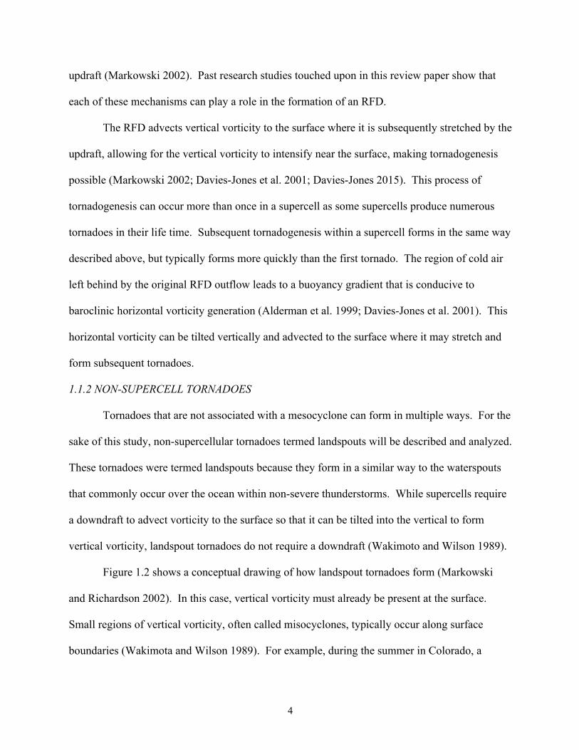
updraft (Markowski 2002). Past research studies touched upon in this review paper show that

each of these mechanisms can play a role in the formation of an RFD.

The RFD advects vertical vorticity to the surface where it is subsequently stretched by the

updraft, allowing for the vertical vorticity to intensify near the surface, making tornadogenesis

possible (Markowski 2002; Davies-Jones et al. 2001; Davies-Jones 2015). This process of

tornadogenesis can occur more than once in a supercell as some supercells produce numerous

tornadoes in their life time. Subsequent tornadogenesis within a supercell forms in the same way

described above, but typically forms more quickly than the first tornado. The region of cold air

left behind by the original RFD outflow leads to a buoyancy gradient that is conducive to

baroclinic horizontal vorticity generation (Alderman et al. 1999; Davies-Jones et al. 2001). This

horizontal vorticity can be tilted vertically and advected to the surface where it may stretch and

form subsequent tornadoes.

1.1.2 NON-SUPERCELL TORNADOES

Tornadoes that are not associated with a mesocyclone can form in multiple ways. For the

sake of this study, non-supercellular tornadoes termed landspouts will be described and analyzed.

These tornadoes were termed landspouts because they form in a similar way to the waterspouts

that commonly occur over the ocean within non-severe thunderstorms. While supercells require

a downdraft to advect vorticity to the surface so that it can be tilted into the vertical to form

vertical vorticity, landspout tornadoes do not require a downdraft (Wakimoto and Wilson 1989).

Figure 1.2 shows a conceptual drawing of how landspout tornadoes form (Markowski

and Richardson 2002). In this case, vertical vorticity must already be present at the surface.

Small regions of vertical vorticity, often called misocyclones, typically occur along surface

boundaries (Wakimota and Wilson 1989). For example, during the summer in Colorado, a

5

convergence and vorticity boundary coined the “Denver Convergence and Vorticity Zone” or

“DCVZ” often sets up near the Denver International airport (Szoke et al. 1984; Brady and Szoke

1989). This boundary forms when southeasterly winds interact with the topography to create a

cyclonic feature that produces a region of convergence. Within this line of convergence, small

misocyclones can be embedded. This mesoscale set up makes Colorado a region where

landspouts are relatively common.

In order to create a tornado out of a misocyclone, vertical vorticity at the surface must be

drawn upward. This occurs when the updraft of a developing storm moves over a misocyclone.

The updraft stretches the vertical vorticity, causing it to be drawn upward and to increase in

intensity as its radius decreases (Wakimoto and Wilson 1989). Because the landspout forms

directly from an updraft stretching vertical vorticity, the tornado is completely dependent on the

strength of the updraft. Typically, these tornadoes form in ordinary thunderstorms, far from a

severe classification. Once a downdraft begins to develop and precipitation begins to fall,

choking off the updraft, the landspout typically diminishes. Though these landspouts are often

not as long lived or as strong as their supercellular counterparts, they are still able to cause costly

damage to structures and endanger people’s lives. The strong winds found within a landspout

make for very dangerous aviation conditions, causing these landspouts to be of great interest to

forecasters.

1.2 LIGHTNING CHARGE SEPARATION

Lightning is considered to result from charge separation within the mixed phase region of

a convective cloud. Typically, this charge separation manifests itself as a normal tripole charge

structure characterized by mid-level negative charge that is situated between an upper and lower

region of positive charge (Williams 1989). The physical mechanisms that create this charge

6

structure have been the focus of numerous laboratory studies (Reynolds et al. 1957; Takahashi,

1978; Jayaratne et al. 1983; Baker et al. 1987; Saunders et al. 1991; Saunders and Brooks 1992;

Saunders and Peck 1998; Mason and Dash 1999, 2000). Reynolds et al. (1957) was the first to

find that significant charge separation occurs when a simulated graupel particle undergoing

riming collides with ice crystals in the presence of supercooled liquid water.

In a similar laboratory study, Takahashi (1978) discovered that the sign of charging on

graupel was highly dependent on the ambient temperature and the cloud liquid water content. At

temperatures colder than -10℃, graupel charged negatively while ice crystals charged positively.

Takahashi also established that this charge reversal temperature was dependent on the

supercooled liquid water content. Positively charged small ice crystals are lofted to high

altitudes, creating an upper positive charge region. Large graupel particles possess significant

terminal velocities which allows these particles to fall to lower altitudes within a cloud. As

graupel particles fall, many particles reach a balance level in which their terminal velocities are

matched by the updraft velocities, leading to a stratified region of negative charge at mid-levels

of the storm formed by the levitated graupel (Lhermitte and Williams 1985). Observations of

thunderstorms have revealed that this mid-level negative charge layer tends to center somewhere

between -10℃ and -20℃ (Dye et al. 1986).

Takahashi (1978) found that the sign of graupel charging reversed to positive below the

so-called charge reversal temperature of -10℃.##This positive charging of graupel would explain

the lower positive charge region found in a thunderstorm tripole charge structure. Jayaratne et

al. (1983) found that the charge reversal occurred at -20℃. Continued laboratory experiments

have shown that graupel can also charge negatively at temperatures warmer than -10℃ when

cloud liquid water contents are extremely small. These studies have also discovered that graupel

7

charges positively at extremely large liquid water contents (Saunders et al. 1991; Saunders and

Peck 1998).

While laboratory studies agree that graupel can charge both positively and negatively

within a cloud, the mechanism that allows for this charge reversal is still a topic of debate.

Saunders et al. 2008 summarizes the various proposed mechanisms that have been disproven

over the years. The non-inductive charging mechanism is the currently accepted theory for

charge separation within thunderstorms. Baker and Dash (1994) suggest that a quasi-liquid layer

(QLL) surrounding an ice particle is responsible for the transfer of charge via the non-inductive

charging mechanism. This layer exhibits outward negative charge because OH- ions are less

mobile than H+ ions. H

+ ions bury themselves in the ice lattice, while OH

- ions remain within

the thin quasi-liquid layer.

When an ice crystal and graupel particle collide, the QLL’s of each particle intersect and

interact (Dash et al. 2001). Particles growing fastest via vapor deposition maintain a thicker

QLL. During collision, the QLL’s quickly attempt to reach an equilibrium, resulting in the

transfer of mass from the thicker QLL to the thinner QLL, or a QLL of higher chemical potential

to smaller chemical potential. The contact time between the particles is just long enough for the

negative charge within the thicker QLL to transfer to the particle with a thinner QLL, but not

long enough for the positive charge to transfer as well (Dash et al. 2001). Baker and Dash

(1994) state that because of the difference in chemical potential, negative charge is typically

transferred from warm to cold, from higher surface curvature to lower surface curvature, and

from high vapor growth to low vapor growth.

At higher altitudes where the liquid water content is limited, graupel is typically in a

state of sublimation. Because graupel does not grow quickly via vapor deposition compared to

8

ice crystals, ice crystals will display a thicker QLL. When the particles collide, matter from the

thicker QLL is transferred to the thinner QLL found on graupel. Thus the graupel gains negative

charge at upper levels (Dash et al. 2001). At altitudes where the temperature is warmer than the

charge reversal temperature, graupel must charge positively. Multiple studies attribute this

positive charging to graupel growing via wet growth at warmer temperatures (e.g. Takahashi

1978). This would allow the graupel particles to maintain larger QLL’s and to transfer mass to

the ice crystals, reversing the charging process. Saunders and Brooks (1992) found that charging

due to collisions with particles undergoing wet growth is not substantial enough to generate

charge strong enough to induce lightning. Saunders and Peck (1998) suggest that positive

charging on graupel may result from ice filament breaking off of growing graupel. In this case,

graupel grows via vapor deposition in a high liquid water content environment. The filaments

that extend out from the graupel due to accretion to the graupel’s surface exhibit warmer

temperatures at the ends of the filaments due to latent heat released from vapor deposition. OH-

ions concentrate in the warmer outer section while more mobile H+ move closer to the parent

graupel particle. Collisions with ice crystals cause the ends of the filament to break off, leaving

the graupel charged positively. Scientists continue to debate the charging mechanism in

thunderstorms.

The tripole charge structure promotes intra-cloud (IC) flashes between the mid-level

negative charge layer and the upper and lower positive charge layers. It also creates an

environment conducive for negative polarity ground strikes (-CGs). Though –CG’s make up a

majority of the ground strikes found in storms across the United State, certain regions and types

of storms promote the occurrence of numerous positive polarity ground strikes (+CG’s;

Boccippio et al. 2001; Carey et al. 2003; Williams et al. 2005; Fuchs et al. 2015). Boccippio et

9

al. (2001) found that climatologically, the High Plains of the United States produce more +CG’s

than any other region in the country. Multiple studies have also shown that +CG’s are

commonly found to dominate the ground strike polarity in severe storms (e.g. Branick and

Doswell 1992; Carey and Rutledge 1998; Lang et al. 2002, 2004; Carey et al. 2003; Wiens et al.

2005; Tessendorf et al. 2007). The formation of +CG’s has been linked to an “inverted” or

“anomalous” charge structure that is characterized by a mid-level positive charge layer typically

found around -15℃ to -20℃ with a negative charge region positioned above it (Carey and

Rutledge 1998; Weins et al. 2005; Tessendorf et al. 2007; Fuchs et al. 2015).

The physical mechanism as to how this charge structure sets up is still largely unknown.

Since +CG’s typically occur in the High Plains within severe storms, there must be a specific

type of storm morphology or environmental characteristic that is unique to this region. Williams

et al. (2005) hypothesizes that high cloud base heights and corresponding small warm cloud

depths could explain why this region commonly observes anomalous storms. The authors

explain that small warm cloud depths promote more efficient ice production above the freezing

level because more liquid water is lofted into the mixed phase. This occurs because a shorter

warm cloud depth results in less efficient warm rain processes. Higher cloud base heights also

promote broader, more intense updrafts that are subject to less entrainment of dry air into the

cloud (McCarthy 1974). Broader updrafts in combination with less entrainment and enhanced

lofting of liquid water above the freezing level lead to enhanced supercooled liquid water

contents in the mixed phase region of the cloud, which is known to promote positive charging on

graupel (Saunders et al. 1991; Saunders and Peck 1998). Fuchs et al. (2015) confirms this

hypothesis and shows that Colorado is unique in that it produces predominantly anomalous

10

polarity storms, while regions such as Alabama typically only produce anomalous polarity

storms in severe weather.

A thunderstorm does not need to be anomalous to produce +CG flashes. An “end-of-

storm-oscillation” or “EOSO” sometimes occurs during the decaying portion of a storm (Marshal

and Lin 1992; Williams et al. 1994; Pawar and Kamra 2007; Marshal et al. 2009). An EOSO is

characterized by a change in the electric field as a storm dissipates. A typical normal polarity

tripole thunderstorm is dominated by negative charge overhead, with a positive charge layer

situated above and below the main negative charge region. Sometimes a small layer of negative

charge can be found above the tripole. During an EOSO, the main negative charge becomes less

prominent and positive charge dominates the cloud for a period. The electric field within the

thundercloud then switches back to being dominated by negative charge before the storm

completely dissipates. The dominance of positive charge within a cloud is conducive for +CG

production.

The way in which the positive charge comes to dominate the cloud is still a topic of

debate in the literature. Williams et al. (1994) suggests that an inverted dipole charge structure

sets up because of a change in the charging on hydrometeors through the non-inductive charging

mechanism as storm dynamics change in the dissipation stage. Marshal et al. (2009) suggests

that the polarity changes primarily result from the fallout of charge as hydrometeors fall through

the cloud. The study then goes on to explain that the switch back to mainly negative charge

overhead results from the upper negative charge layer that formed above the tripole structure

falling to lower levels. This occurs as the positive charge regions fall to the ground behind the

initial fallout of the main negative charge region. Further study is required to fully understand

11

how EOSO’s occur, but overall it is well accepted that they only occur during the dissipation

phase of a storm.

1.3 LIGHTNING OBSERVATIONS IN SEVERE STORMS

Total lightning flash rates (intra-cloud and cloud-to-ground flashes combined) are closely

related to the characteristics of a storm’s updraft (Goodman et al. 1988; Dye et al. 1989; Carey

and Rutledge 1994; Williams et al. 1999; Lang and Rutledge 2002; Wiens et al. 2005;

Tessendorf et al. 2007; Deierling et al. 2008; Schultz et al. 2015, 2017). Deierling and Petersen

(2008) showed that larger updraft volumes with stronger updrafts lead to a larger production of

graupel and ice crystals in the mixed phase region of the cloud. With more graupel and ice

crystals available, there is greater opportunity for collisions and thus charge separation to occur

via the non-inductive charging mechanism. There have been multiple reports of “lightning

holes” in the literature, in which lightning is virtually non-existent within the strongest portions

of the updraft (e.g. Krehbiel et al. 2000; Wiens et al. 2005; Steiger et al. 2007). Studies show

this occurs because intense updrafts limit the time for small particles to grow into modest size

precipitation particles. The majority of the collisions between particles occurs along the

periphery of the main updraft, where graupel is able to descend and collide with ice crystals as

they ascend to higher altitudes. This mechanism is supported by numerous case study analyses

that have found increases in total lightning flash rate are more highly correlated with updraft

volume than the maximum updraft speed (Deierling and Petersen 2008; Schultz et al. 2015,

2017). The size of lightning discharges is typically small near the updraft, as turbulence leads to

small pockets of intense charge separation (Bruning and MacGorman 2013). Thus, the mean

flash size has been found to decrease as updrafts intensify and flash rates increase (Schultz et al.

2015).

12

Due to the strong observed correlation between the total lightning flash rate and the

updraft strength in a storm, lightning can be useful for nowcasting severe weather. Rapid

increases in lightning flash rates are termed “lightning jumps” (Williams et al. 1999). Total

lightning jumps typically form before the onset of severe weather because they accompany a

rapid intensification of the updraft (Williams et al. 1999; Gatlin and Goodman 2010; Schultz et

al. 2011, 2015, 2017). Total lightning jump algorithms attempt to automate the detection of

these flash rate increases in an effort to earlier predict the occurrence of severe weather (Gatlin

and Goodman 2010; Schultz et al. 2011, 2015, 2017). These algorithms have proven successful

in identifying potentially severe storms.

Though total lightning jumps (both IC and CG flashes included) are useful in identifying

intensifying storms that may produce severe weather, they require other atmospheric data to help

determine what type of severe weather may form. Previous studies have attempted to relate the

occurrence of CG flashes with tornadogenesis, but have not succeeded in finding a robust trend

that could be useful in nowcasting tornadic activity (Perez et al. 1997; MacGorman et al. 1989;

Keighton et al. 1991; MacGorman and Nielsen 1991, Strader and Ashley 2014). Metzger and

Nuss (2013) attempted to compare and relate trends in IC and CG flash rates to different types of

severe weather. Some weak trends were observed, but overall there is still a large lack of

understanding of how total lightning can be used to predict specific types of severe weather. In

an effort to build upon this knowledge base, this study will focus specifically on the relationship

between tornadic storms and lightning characteristics.

Multiple studies have analyzed how total lightning flash rates produced by tornadic

supercells change with respect to the timing of tornadogenesis (Williams et al. 1999; Buechler et

al. 2000; Goodman et al. 2005; Steiger et al. 2005; Steiger et al. 2007; Darden et al. 2010; White

13

et al. 2012; Stano et al. 2014). Each of these studies have found that total lightning flash rates

“jump” well before a tornado is reported. Many of these studies also observed a decrease in the

flash rate as a tornado reached the surface. Williams et al. (1999) attributes this decrease in total

lighting flash rate to the likely formation of a downdraft that helps to bring vorticity to the

surface for tornadogenesis. The height at which lighting occurs within a cloud has also shown

promise in helping to determine information about storm dynamics. Steiger et al. (2005, 2007)

found that lightning flashes occurred at the highest altitudes when the storms analyzed were most

intense. The flashes tended to descend in height during the onset of a tornado. It is hypothesized

that this descent results from an updraft weakening/downdraft formation.

1.4 GOALS OF THIS STUDY

There is proven utility in monitoring total lightning flash rates during severe weather

nowcasting operations. The relationship of lightning to updraft intensification is apparent, but

the way in which the dynamics that produce severe weather affect lightning are less understood.

Lightning jumps provide evidence of an intensifying storm, but they do not provide any

indication of what will happen after the storm intensifies. The storm could produce hail, strong

winds, tornadoes, or no severe weather at all. This study takes a step away from the lightning

jump framework to take a more in depth look at how lightning evolves with the evolution of

severe storms. Specifically, this study seeks to understand how tornadogenesis relates to

changes in lightning characteristics. The following questions are addressed:

1)! How do flash rates react to the onset of a tornado at the surface? Does the type of

tornadogenesis (i.e. supercellular vs. landspout tornadogenesis) change these results?

2)! Do other lightning characteristics, such as the height of the lightning flashes or the

occurrence of CG flashes, reveal information about the evolution of tornadic storms?

14

3)! How does the environmental regime affect the lightning characteristics? Specifically,

how does lightning differ between tornadic storms in Alabama and Colorado?

Detailed case study analysis of a number of lightning producing tornadic storms are

analyzed to seek answers to these questions. The total lightning flash rate, CG flash polarity, and

location of lightning flashes with regard to altitude are analyzed in each case. To address the

difference between lightning in different environmental regimes, two supercells are analyzed in

the dry, high cloud base height environment in the High Plains (Colorado) and two supercells are

analyzed in the warm, humid, low cloud base height environment found in Alabama. To

understand how differing forms of tornadogenesis affect lighting characteristics, lighting

produced by supercells is compared to lightning produced by landspouts. This analysis only

studies six tornadic storms, so the results are not robust by any means. By taking a close look at

individual storms, this study looks to bring an awareness of what may be controlling the

changing lightning characteristics within evolving severe storms.

15

Figure 1.1 Visual depiction of supercellular tornadogenesis taken from Markowski and Richardson (2009).

a) horizontal vorticity vortex tubes set up as result of environmental shear, b) an updraft lifts these vortex

tubes upwards, c) upward tilting of the vortex tubes creates vertical vorticity at upper levels, creating a

rotating updraft, d) a downdraft advects vertical vorticity to the surface as horizontal vorticity continues to

be turned into the vertical e) vertical vorticity advected to the surface is stretched by the updraft and

enhanced, allowing for tornadogenesis to occur

16

Figure 1.2 Visual depiction of landspout formation taken from Markowski and Richardson (2009). a) vertical

vorticity is present at the surface, b) an updraft from a developing storm moves over a region of confined vertical

vorticity at the surface, c) the updraft stretches a region of vertical vorticity upwards, d) vertical vorticity is

enhanced by stretching, e) vertical vorticity converges underneath the updraft, allowing for tornadogenesis

17

CHAPTER 2: DATA AND METHODOLOGY

2.1 RADAR DATA

2.1.1 NEXRAD WSR-88D RADARS

The Next Generation Weather Radar (NEXRAD) program was created to develop and

deploy an advanced network of WSR-88D’s (Weather Surveillance Radar- 1988 Doppler)

throughout the United States (Crum and Alberty 1993). These radars are run 24 hours a day and

are used primarily by the National Weather Service (NWS) for forecasting and severe weather

warning purposes. The WSR-88D network is comprised of S-band radars that simultaneously

transmit and receive both horizontally polarized (H) and vertically polarized (V) electromagnetic

radiation (Doviak et al. 2000). Radar volumes are made up of 360 º azimuthal scans with

varying elevation angles. Multiple predefined scan strategies can be utilized to create these

volumes based on operational need (Crum and Alberty 1993). WSR-88D data is available for

free download for any radar site in the network at https://www.ncdc.noaa.gov/nexradinv/.

This study utilizes WSR-88D data from the KFTG site in Denver, CO and the KHTX site

in Huntsville, AL. Radar data output utilized in this study include reflectivity (Z), aliased radial

velocity (Vr), and differential reflectivity (ZDR). The radial velocity field is dealiased using the

Python ARM-Radar Toolkit (Pyart; Helmus and Collis 2016). Pyart has multiple automated

dealiasing algorithms that can be used to correct the data. Visual inspection of the data after

running the radial velocity fields through two of these automatic dealiasing algorithms show that

these algorithms are able to correctly unfold the velocity fields. To remove clutter and unwanted

reflectivity echoes resulting from non-meteorological objects, the data are thresholded using the

standard deviation of differential phase (SDP) and the cross-correlation coefficient ($%&)

18

(Ryzhkov and Zrnic 1998). After dealiasing and decluttering the data, the radar data are then

further quality controlled and specific differential phase (KDP) is calculated utilizing the Dual-

Polarization Radar Operational Processing System (DROPS), described by Chen et al. (2017).

This system calculates KDP through the Wang and Chandrasekar (2009) method. The data are

then gridded to a Cartesian coordinate system.

2.1.2 CSU-CHILL RADAR

The Colorado State University -!University of Chicago–Illinois State Water Survey

(CSU-CHILL) National Radar Facility (Brunkow et al. 2000) is located in Greeley, Colorado.

This state of the art research weather radar supports full polarimetric radar operation at both S-

band (11.01 cm) and X-band (3.18 cm). S-band operations are characterized by a 1º beamwidth

and X-band operations are characterized by a 0.3º beamwidth. The radar is capable of both

simultaneous and alternating transmission of H and V at S-band (alternating at S-band only). S-

band and X-band operations can be run simultaneously, or in a single frequency configuration.

This study utilizes S-band data for one of the Colorado cases. Because the CSU-CHILL

radar is a research weather radar, it performs fully configurable surveillance scans, plan-position

indicator (PPI) scans, and range height indicator (RHI) scans as commanded. RHI scans display

vertical cross sections through a storm at a specified azimuth at a much higher resolution than

gridded radar volume data can provide. CSU-CHILL data output includes Z, aliased Vr, KDP,

and ZDR and co-polar correlation coefficient. Similar to the NEXRAD WSR-88D data, the

radial velocity fields were dealiased using Pyart automatic dealiasing algorithms and quality

controlled by thresholding based on SDP and $%&.

19

2.1.3 ARMOR RADAR

The Advanced Radar for Meteorological and Operational Research (ARMOR) is located

in Huntsville, AL. This C-band (5.33 cm) polarimetric radar transmits H and V simultaneously.

The beamwidth is 1.0 º. Radar variables of interest output by ARMOR include Z, aliased Vr,

and ZDR. The data were quality controlled using DROPS and thresholded based on SDP and

$%&. The radial velocity field was dealiased by first running the data through the automatic

unfolding algorithms used for both the WSR-88D and CSU-CHILL data. Due to the smaller

Nyquist velocity that results from using C-band, the velocity field was more severely aliased

than data produced by the S-band radars. The automatic dealiasing algorithms were not able to

completely unfold the radial velocity fields, so the data was subjectively analyzed and manually

unfolded utilizing the ARM Radar Toolkit Viewer (ARTview; https://github.com/nguy/artview).

The data is then gridded to a Cartesian coordinate system.

2.2 CLEAR FRAMEWORK

The Colorado State University (CSU) Lightning, Environment, Aerosols, and Radar

(CLEAR) framework described in Lang and Rutledge (2011) was used to identify convective

cells and track them throughout their lifetime. CLEAR takes in gridded three-dimensional radar

data, determines the composite reflectivity values for each x-y grid point, and then uses

reflectivity and spatial thresholds to identify convective features within the composite reflectivity

field. For example, five of the six cases in this study required that each convective cell maintain

a 35 dBZ composite reflectivity contour of at least 20 km2 in horizontal area and a 45 dBZ

contour of at least 10 km2 in area. Due to the small spatial area and weak reflectivity of one of

the landspout cases, these thresholds were reduced to 30 dBZ for 10 km2 and 40 dBZ for 5 km

2.

20

The features identified by CLEAR are assigned storm tracks that can be referenced for

further analysis. The program is also able to take in other data, such as environmental sounding

data, and attribute it to each of these storm cells. CLEAR outputs the original input radar files

with newly added storm cell and storm track information. If other data were included, this data

is attributed as well.

CLEAR does not always perfectly attribute cells to storm tracks. Sometimes CLEAR

picks up on a storm track and ends it prematurely. As a result, a subjective analysis of the storm

cell and track information was performed to determine exactly which tracks made up the storms

of interest. To ensure that the data analyzed for each storm of interest came exclusively from

that storm, all data outside of the 35 dBZ composite reflectivity contour defined by CLEAR were

masked out. The area of the 35 dBZ contour was applied to the vertical by extending the contour

level upward through each vertical level.

2.3 RADAR ANALYSIS

2.3.1 POLARIMETRIC VARIABLES

Z, Vr, ZDR, and KDP were analyzed in this study in both horizontal and vertical cross

sections for each case study storm. ZDR represents the difference between the horizontal

reflectivity factor and vertical reflectivity factor (or the ratios of these two powers expressed as a

log quantity). Positive ZDR values are characterized by hydrometeors that are larger in the

horizontal compared to the vertical, such as oblate, falling raindrops. Spherical targets display

ZDR of near zero. ZDR is biased towards larger particles since it is a reflectivity-weighted

measurement. KDP is similar to ZDR in that positive values represent oblate hydrometeors. But

unlike ZDR, KDP is dependent on mass content as well as oblateness. Larger values of KDP

indicate a higher concentration of rain. Thus large Z values collocated with large KDP indicate

21

heavy rain. Small (near zero, or zero) ZDR and KDP values within a region of large Z indicate

the presence of tumbling hail. When rain is mixed with hail, ZDR will be depressed towards

zero but KDP will be non-zero and positive.

Analyzing vertical cross sections of polarimetric data through the updraft region of a

storm can reveal valuable information about updraft strength and storm maturity. On a basic

level, enhanced convergence at the surface and divergence aloft depict a strong updraft. If Z

values are small along the region of convergence, this indicates the presence of a bounded-weak

echo region (BWER). In this case, an intense updraft lofts small hydrometeors through the

region of convergence, resulting in very little time for particles to grow to sizes detectable by

radar.

Enhanced values of ZDR and KDP above the freezing level, termed ZDR and KDP

columns, also indicate a strong updraft (Kumjian and Ryzhkov 2008). ZDR columns represent

the presence of large water droplets produced by warm rain processes. Large drops can also be

formed via the melting of hail and subsequently transported upward in the updraft. KDP

columns (positive KDP) indicate the lofting of oblate drops as well.

2.3.2 HYDROMETEOR ANALYSIS

Hydrometeor identification (HID) is performed using the CSU-Radartools fuzzy logic

hydrometeor identification program (https://github.com/CSU-Radarmet/CSU_RadarTools). This

program takes in gridded radar data and uses Z, ZDR, KDP, and the cross-correlation ratio to

determine what particular hydrometeor type is dominant at each grid point. The radar data for

each case is gridded using a 1 km x 1 km x 1 km grid-spacing. The graupel volume above the

freezing level of the storm of interest is derived for each radar volume. Lightning production

relies on the formation of graupel and ice crystals in the mixed phase region. Analysis is limited

22

to regions above the freezing level so that graupel falling out of the cloud does not distort the

visualization of in cloud graupel volume and its relationship to lightning characteristics over

time. Freezing levels are determined through analyzing atmospheric soundings available in the

University of Wyoming atmospheric sounding archive

(weather.uwyo.edu/upperair/sounding.html). Graupel volume is calculated by simply summing

the number of grid boxes within the storm cell of interest that contain predominantly graupel

above the freezing level (derived from the HID algorithm). This value is recorded for each radar

volume and then displayed as a time series so that that the change in graupel volume throughout

the evolution of the storm can be visualized. The same methodology is applied to calculate the

hail volume.

A reflectivity – mass relationship (or Z-M) is used to determine the mass of graupel and

hail within the storm at each radar volume. Graupel mass is calculated using the same Z-M

relationship used in Schultz et al. (2015). This relationship shown in (1) is originally derived by

Heymsfield and Miller (1988). “z” represents the linear reflectivity factor in mm6 m

-3.

'( # )#*+, = 0.0052#×#23.4 (1)

The Z-M relation is applied to each grid point within the storm cell that is identified to be

predominantly graupel. The mass values calculated at each grid point are then summed and

recorded to create the total graupel mass for that volume. This is done for each radar volume and

displayed in a time series. The same methodology is applied for calculating the hail volume, but

a different Z-M relationship (2) is used (Cheng and English 1983; Carey and Rutledge 1996;

Lopez and Aubagnac 1997). ZH is the reflectivity factor due to hail in mm6 m

-3 and $% is the

density of hail, taken to be 900 kg m-3

.

'% # )#*+, = 104.21#×#10+7#$%8%

3.93:;

23

The CSU-Radartools blended rain algorithm is used to calculate the conditional rain rate

for each storm cell over time (https://github.com/CSU-Radarmet/CSU_RadarTools). This

algorithm utilizes output from HID analysis to determine where ice is present so that rain rates

are not contaminated by the presence of ice. The average conditional rain rate is calculated by

masking out all rain rates of 0 mm hr-1

and then taking the average of the resulting data field

within the 35 dBZ contour defined by CLEAR.

2.3.3 DUAL-DOPPLER ANALYSIS

The ARMOR radar is located in close proximity to the KHTX WSR-88D. For a period

in both the Alabama supercells, radar data from ARMOR is available to complete dual-Doppler

analysis. Radial velocity only measures two components of the wind field, making it so that the

vertical component of the wind field cannot be determined from one radar alone. Through using

radial velocity values observed by two radars, the 3-D wind field can be determined through

solving the mass-continuity equation for vertical motion with appropriate boundary conditions

for the integration (Lhermitte 1968; Armijo 1969).

To accurately retrieve the vertical velocity within a storm, the fall speed of hydrometeors

must be accounted for when solving the mass-continuity equation. Using a simple hydrometeor

identification algorithm that determines where rain, graupel, and snow occur in a cloud, a fall

speed is calculated for each grid point in the radar file being analyzed. The fall speeds are

calculated based on the reflectivity utilizing relationships defined in Giangrande et al. (2013).

Radar volumes used for each dual-Doppler retrieval may not occur simultaneously. Storm

advection between volumes is manually determined and accounted for as well.

The Custom Editing and Display of Reduced Information in Cartesian Space (CEDRIC)

software is used to synthesize the radar data and produce a 3-D wind field (Mohr et al. 1986).

24

This program takes in gridded radar data from two radars, as well as storm advection and

hydrometeor fall speed information, and solves the mass-continuity equation. The time periods

in which ARMOR data is available for dual-Doppler analysis are not long enough for useful

information to be gained by calculating updraft speeds and volumes, as past studies have done

(e.g., Schultz et al. 2015). In the April 27, 2011 supercell case, ARMOR was switched from

completing research oriented high-resolution sector scans to low level surveillance scans to assist

the NWS in their severe weather nowcasting efforts on that day. The 3-D wind field is used

instead to add wind vectors to radar cross sections during the Alabama supercells so that the

updraft intensity can be visualized in conjunction with other polarimetric variables.

2.4 LIGHTNING DATA

2.4.1 LIGHTNING MAPPING ARRAY

A lightning mapping array (LMA) is a network of sensors that use GPS time of arrival

techniques to locate sources of VHF radiation emitted by lightning in space and time (Rison et

al., 1999, Krehbiel et al., 2000). LMAs detect radiation at frequencies of 60-66 MHz. By

knowing exactly where in space these sources originate from, LMA source data can be used to

map lightning channels and infer the internal charge structure of a storm. Negative breakdown

within a positive charge layer produces larger amounts of radiation compared to positive

breakdown in a negative charge layer (Rison et al., 1999). Altitudes that contain higher LMA

source densities are inferred to be positive charge regions due to the noisier breakdown in these

regions (Wiens et al. 2005; Tessendorf et al. 2007; Lang and Rutledge 2011; Fuchs et al. 2015).

The Colorado LMA (COLMA) and North Alabama LMA (NALMA) are utilized in this

analysis. Sensitivity studies in Fuchs et al. (2015) show that COLMA is a more sensitive

network because it has more stations and a lower noise floor than NALMA. Both COLMA and

25

NALMA become less sensitive moving away from the network center (Fuchs et al. 2015), as

expected due to the 1/r2 law. In order to affirm that accurate source counts are recorded for each

LMA, storms are only analyzed when they are within 100 km of the NALMA network center

and 125 km of the COLMA network center. COLMA is a larger, more sensitive network,

making it so that detection is accurate at a further range.

2.4.2 NATIONAL LIGHTNING DETECTION NETWORK

The National Lightning Detection Network (NLDN) detects radiation in the VLF (3-30

kHz)/LF (30-300 kHz), throughout the entire United States at a 90-95% detection efficiency

(Cummins et al. 1998; Cummins and Murphy 2009). Lower frequencies are not able to detect

smaller IC flashes well, but are very good at detecting CG flashes and their corresponding return

strokes. IC and CG flashes detected by NLDN are differentiated through waveform analysis.

Through recommendations by Dr. Timothy Lang (personal communication), all flashes classified

as CG that produced peak currents less than 15 kA were considered IC flashes. If an IC flash

produced a peak current greater than 25 kA, the flash was recorded as a CG flash.

2.5 FLASH CLUSTERING AND ATTRIBUTION

An open source flash clustering algorithm described in detail by Fuchs et al. (2015) is

utilized to group LMA sources into flashes. The algorithm also attributes LMA and NLDN flash

information to the cells previously defined by the CLEAR framework. LMA and NLDN flashes

that are within 10 km of the storm cell are attributed to each individual cell. Before sources are

clustered into flashes, they are thresholded based on the number of sensors that detected each

source. COLMA sources are required to be detected by 7 or more sensors to be applied to the

clustering algorithm. Due to the fewer number of sensors and the decreased sensitivity, 6 or

more stations are required for NALMA sources (Fuchs et al. 2015).

26

Numerous parameters are considered when sources are clustered together to create a

flash. First, a minimum number of sources per flash is defined. For Colorado storms, 10 sources

are required. For the less sensitive Alabama network, 5 sources are required. Five sources was

chosen for Alabama because this value produced the most reasonable supercell flash rates when

compared to typical flash rates found in the literature (e.g., Goodman et al. 2005; Gatlin and

Goodman 2010; Schultz et al. 2011). A 10 source minimum was tried first, but this parameter

resulted in more NLDN CG flashes being detected than total lightning LMA flashes during

certain time periods, which is not reasonable. A 2 source minimum was also tried, but this

solution created unreasonably high flash rates. Wiens et al. (2005) demonstrates that the choice

in minimum sources does not change the overall trend of the flash rates produced. Results from

testing various minimum source parameters for NALMA confirmed this idea.

To create a flash, the minimum number of sources must be defined within specific spatial

and temporal thresholds. For both NALMA and COLMA the spatial threshold requires each

source in a cluster be within 3 km of one another. Each source cannot be further than 0.15 s

apart in time of occurrence as well. Once the minimum number of sources is reached such that

these spatial and temporal criteria are met, the program looks for more sources to attribute to that

flash. If no sources are available within the proper distance and time threshold, a new search

begins for a new flash.

2.6 LIGHTNING ANALYSIS METHODOLOGY

LMA flashes are used to create total lightning flash rates, with the assumption that the

LMA sees all CG and IC flashes with 100% detection efficiency. The evolution of total

lightning flash rates is determined by combining the flashes attributed to every radar volume

storm cell within the storm track of interest. These combined flashes are binned into 1-minute

27

intervals. The number of flashes within each bin is recorded and then displayed in a time series

such that the total lightning flash rate at each minute of the analysis period is displayed.

To monitor the evolution of the charge structure in each case study, a source density

analysis is completed for each case. To do this, the LMA sources attributed to the relevant storm

cell in each radar volume are binned into 0.5 km vertical intervals. The number of sources

within each vertical level is counted and divided by the total number of sources in the storm cell.

The percent of sources that occur at each height interval within the storm cell is revealed. This

analysis is repeated for each radar volume. The results for each radar volume are combined to

create a time series of these source densities. Each row of a source density plot represents a

height interval and each column represents a storm cell (or radar volume) within the storm track

of the case.

Each of the supercellular cases also contain a CG flash polarity analysis. The landspout

cases produced no CG flashes. Corrected NLDN CG flashes are attributed to each radar volume

through the flash clustering algorithm described above. Much like the total lightning analysis,

the flashes attributed to each storm cell/radar volume throughout the entire storm track of interest

are grouped together and binned in 1-minute intervals. The bins are broken up into +CG and –

CG flash bins. The number of +CG and –CG flashes that occur within each bin are counted and

recorded. A time series of 60 s +CG flash rates and –CG flash rates throughout the duration of

the storm is displayed.

2.7 IR MINIMUM BRIGHTNESS TEMPERATURES

Super Rapid Scan Operation for GOES-R (SRSOR) produced 1-minute scans of satellite

imagery taken from GOES-14. This scan mode was a part of the GOES-R Proving Ground that

was created to help prepare forecasters and atmospheric researchers for the capabilities that

28

GOES-R would provide through the creation of the Advanced Baseline Imager (ABI) (Schmit et

al. 2005). This study utilizes 10.7<* infrared (IR) data from SRSOR operations on June 4, 2015

to determine how the minimum brightness temperature over the overshooting top of the storm of

interest on this day changed with time.

IR data is corrected for parallax using code written by Dr. Steven Miller (personal

communication) that follows the methodology outlined in Vincente et al. (2002). IR data is

interpolated to a 200 by 200 grid with 0.02° grid spacing in x (longitude) and y (latitude). A box

encompassing the June 4 overshooting top is then defined from 105.5°W to 104.2°W and 39.7°N

to 40.5°N such that any data outside of this region is masked out. This is done to ensure that no

other overshooting tops from nearby storms adversely impact this analysis. The minimum

brightness temperature within this box was recorded for each 60 s file. These minutely minimum

brightness temperatures were then combined to create a time series of the minimum cloud top

brightness temperature over the overshooting top. It should be noted that convective cloud tops

are assumed to be opaque, such that they emit as a blackbody.

!

!

!

!

!

29

CHAPTER 3: RESULTS

3.1 COLORADO SUPERCELLS

3.1.1 BERTHOUD SUPERCELL

On June 4, 2015, an EF3 tornado touched down near Berthoud, CO in association with a

supercell that moved westward along the Larimer and Boulder county lines. The tornado was on

the ground from 00:30 to 01:08 UTC and produced maximum wind speeds near 135-140 mph

(Storm Data- available at https://www.ncdc.noaa.gov/stormevents/). This storm was especially

unique to this region because the supercell and the corresponding tornado moved from east to

west, unlike the typical west-to-east motion of storms in this region. The intensity of this

tornado was also unique as only 10% of the tornadoes produced in either Colorado or Wyoming

(from a climatological perspective) are reported as EF3 or greater (Schumacher et al. 2010).

The environmental conditions for this day were conducive for tornadogenesis. Both the

12 UTC and 00 UTC Denver soundings revealed values of Convective Available Potential

Energy (CAPE) near 1500 J kg-1

. The 00Z sounding also showed strongly sheared winds within

the lowest 3 km of the atmosphere. A video analysis completed by Dan Bikos (Cooperative

Institute for Research in the Atmosphere, Colorado State University; available at

http://rammb.cira.colostate.edu/training/visit/blog/index.php/2015/07/17/4-june-2014-goes-1-

minute-visible-imagery-and-time-lapse-video) discusses the patterns revealed by one-minute

visible imagery available from Super Rapid Scan operations for GOES-R (SRSOR) employed on

GOES-14 during the time period of this case. The one-minute visible imagery reveals that the

severe storms on this day initiated from a cumulus field that moved from eastern Colorado

westward and developed into towering cumulus clouds as it approached the Front Range.

30

Outflow boundaries and gravity waves produced by mature storms that had developed earlier in

the day aided in the development of mature convection from the towering cumulus clouds. The

storm of interest, nicknamed the Berthoud supercell, was spawned by this earlier convection.

The Berthoud supercell began as a cluster of multicellular storms over Larimer County.

At approximately 00 UTC, the cluster split into two separate storm cells with the southward

moving cell becoming the Berthoud supercell. The total lightning flash rate sharply increases

from about 20 flashes min-1

to a local maximum of 220 flashes min-1

within the first 15 minutes

of the analysis period (Figure 3.1a). As past studies have found, this rapid increase in flash rate

is indicative of updraft intensification (e.g. Williams et al. 1999; Gatlin and Goodman 2010;

Schultz et al. 2011, 2015, 2017). Figure 3.1b displays CG flash rates distinguished by flash

polarity. While the total lightning flash rates increase within the first 15 minutes of the analysis

period, the CG flash rate remains very small. This suggests that the total lightning flash rate is

dominated by IC flashes as the updraft intensifies. When an updraft intensifies, increased

turbulence leads to enhanced collisions between graupel and ice crystals, creating small pockets

of charge separation along the periphery of the updraft (Bruning and MacGorman 2013). These

small regions of enhanced charge separation lead to the formation of numerous small IC flashes,

resulting in an increased IC flash rate, but not an increased CG flash rate. As a storm initially

intensifies these small flashes may appear to rise in altitude as the storm develops and cloud tops

reach higher altitudes. This can be seen in the LMA source density plot in Figure 3.1c. A slight

rise in the height of the maximum source density occurs as the total lightning flash rate increases.

The beginning of the Berthoud storm is characterized by source densities maximizing around 10

km, which is typical of a normal polarity storm.

31

Visible imagery from SRSOR data supports the idea that the updraft is intensifying

throughout the first 15 minutes of the analysis period. A cauliflower-like texture accompanied

by multiple shadows over a small, discrete portion of the cloud top indicates the presence of an

overshooting top during the beginning of the analysis period (Figure 3.2a). Overshooting tops

occur when an updraft is strong enough to penetrate the equilibrium level (American

Meteorological Society Glossary). To gauge the intensity or strength of this feature, the

minimum brightness temperature above the overshooting top is plotted with respect to time in

Figure 3.3. During the inferred updraft intensification, the cloud top minimum brightness

temperature decreases quickly. This decrease in temperature reveals that the cloud directly

above the updraft is growing in altitude as the updraft penetrates further past the equilibrium

level, reaching colder temperatures. By monitoring the minimum brightness temperature as

opposed to the entire convective region of the cloud top, fluctuations in the updraft intensity can

be inferred. The convective region of a storm will produce rising and falling cloud tops as the

storm intensifies and weakens respectively, but monitoring small scale changes in intensity is

more difficult because the broader convective region is subject to being stopped at the

equilibrium level. By monitoring the portion of the storm directly associated to the updraft that

is able to break through the equilibrium level, it is more likely that small scale changes in updraft

intensity will be revealed.

Cross sections of dual-polarized radar variables show that the Berthoud storm was well

organized with a defined bounded weak echo region (BWER) in the vicinity of the updraft by

00:21 UTC, approximately 9 minutes prior to the initial tornado touch-down (Figure 3.4a). The

updraft is visualized by a region of convergence in the Vr field (Fig. 3.4b). The radar is located

to the southeast of the Berthoud supercell. As a result, regions where blue inbound colors are to

32

the left of the red outbound colors show a region of convergence. An atmospheric sounding

taken in Denver, CO at 00Z shows that the freezing level was slightly lower than 3 km at this

time. Regions of enhanced ZDR values are found above the freezing level in the vicinity of the

updraft (Figure 3.4c). These features are termed “ZDR columns” (Kumjian and Ryzhkov 2008).

ZDR columns depict the lofting of oblate drops above the freezing level associated with a

convective updraft. These drops promote enhanced graupel production because the drops freeze

and accrete supercooled liquid water to create graupel. The KDP field in Figure 3.4d does not

show any noteworthy features at this point in time.

The ZDR column in Figure 3.4c coincides with a period in which the graupel volume and

graupel mass above the freezing level are increasing while the rain rate fluctuates, as depicted in

Figure 3.5. While 00:15 UTC represents a local maximum in the flash rate, the graupel mass and

volume both continue to grow until 00:25 UTC where a local maximum is reached.

Consequently, shortly after 00:25 UTC another local maximum in the flash rate is reached.

Cross sections of ZDR continue to display oblate drops being lofted above the freezing level via

the updraft through 00:26 UTC. The rain rate fluctuates at this time likely as a result of the

storm continually gaining intensity (Figure 3.5a). Just prior to 00:25 UTC, the minimum

brightness temperature above the overshooting top warms rapidly. Investigation of satellite

visible imagery reveals that the cauliflower-like texture also diminishes at this time, suggesting

that the overshooting top collapsed. An example of this change in visible imagery is displayed in

Figure 3.2b. The flash rate and graupel volume also show decreases shortly after 00:25 UTC,

with both parameters reaching local minimums by 00:45 UTC. These changes in storm

characteristics suggest that the updraft has weakened at this time.

33

Overshooting tops must be maintained by a strong updraft, therefore the decrease in the

altitude of the overshooting top is the first sign of updraft weakening. Updrafts tend to weaken

during a storm’s life time as a result of precipitation loading as ice hydrometeors become larger

and heavier. These ice hydrometeors typically fall out of the cloud once their terminal velocity

becomes larger than the updraft speed. This precipitation loading may result in the onset of a

downdraft. The decrease in graupel volume and graupel mass between 00:25 and 00:45 suggests

that graupel is falling below the freezing level. Radar cross sections within this time frame also

show enhanced values of both KDP and ZDR above the freezing level that are not collocated

with the region of convergence that indicates updraft location. Since these values do not occur

within the updraft, they likely indicate oblate droplets shedding off of melting hail while it falls

through the cloud as the updraft weakens. During this same time period, Figure 3.5a shows that

there is a constant increase in the mean conditional rain rate within the Berthoud supercell.

Falling rain leads to evaporative cooling, which encourages downdraft formation as the cooler air

makes the parcel negatively buoyant.

The data suggest that a downdraft formed at approximately 00:25 UTC. This idea is

further supported by the tornado touchdown that occurs at 00:30 UTC. As discussed in Chapter

1, tornado formation within a supercell requires a downdraft to advect vertical vorticity to low

levels in the atmosphere where it can subsequently be ingested into the updraft and stretched to

form enhanced vertical vorticity near the surface. The combination of an increased rain rate,

decrease in graupel volume, and the collapse of an overshooting top all support the idea that a

downdraft has formed, allowing tornadogenesis to take place.

Shortly after the radar-inferred downdraft begins, the lightning source densities fall in

altitude to about 6 km and become denser at a localized altitude rather than being spread out

34

throughout the column. Some severe storms become anomalous as they intensify, but in this

case, the altitude of the highest source density falls as the flash rates and all other updraft

parameters are within a weakening stage. As a result, the lowering of this charge region may be

related to falling of positively charged hydrometeors through the cloud. The non-inductive

charging mechanism causes graupel particles to charge negatively while ice crystals charge

positively, leading to an upper positive charge region and mid-level negative charge region in the

case of a normal polarity storm. The source densities within a storm appear greatest in regions of

positive polarity charge. This occurs because negative breakdown within a region of positive

charge produces more VHF radiation compared to positive charge breakdown in a region of

negative charge, and thus producing more sources for the LMA to record (Rison et al. 1999). As

the graupel mass above the freezing level begins to fall and the rain rate increases, it can be

assumed that the graupel is falling out of the cloud while the ice crystals fall to lower altitudes

due to the now weaker updraft. This scenario would result in a fallout of the negative charge

region and a lowering of the positive charge region. It is interesting to note that this lowering of

charge does not lead to enhanced CG flash production. Rather, CG flash production almost

completely stops during the touchdown of the Berthoud tornado, as shown in Figure 3.1b. Only

IC flashes are produced during this time period.

The Berthoud tornado remains on the ground through 01:08 UTC (~38 min duration).

Before the tornado lifts, there is a sharp increase in the flash rate near 00:55 UTC. The flash rate

continually increases until it reaches a maximum value of nearly 290 flashes min-1

. This

extremely rapid increase in flash rate once again suggests that an updraft is intensifying. Cross

sections of the polarimetric radar variables show that throughout the tornado duration, the

updraft region progressively weakens with KDP and ZDR columns disappearing (Figure 3.6).

35

At 00:48 UTC, the Vr field shows enhanced convergence at low levels and divergence aloft

compared to the previous volumes, suggesting that the updraft is organizing once again. The Vr

fields increase in intensity through 00:54 UTC, just a few minutes before the maximum in flash

rate is established. The increase in convergence and velocity fields suggests that the updraft has

intensified once again as the flash rates increase rapidly.

Shortly after the peak in flash rate, the flash rate drops once again. Cross sections of

polarimetric radar data (not shown) display weakening reflectivity fields along with enhanced

KDP and ZDR at low levels, suggesting the fallout of hydrometeors. The storm also loses it

supercellular structure and begins to form into three separate cells that are in close proximity to

one another. Since the initial decent in LMA source density that occurred during the initial

downdraft formation, the VHF source densities have predominantly been largest at lower

altitudes in the cloud, near 7km. However, beginning at 01:20 UTC, the source densities

transition to predominantly upper levels. During this rise in altitude, the source densities spread

out throughout the storm depth. The flash rates increase during this time period. Radar cross

sections show one of the storm cells producing KDP and ZDR columns. Enhanced KDP values

along the updraft region above the freezing level indicate that oblate drops are being lofted above

the freezing level, just as in ZDR columns (Kumjian and Ryzhkov 2008). The rise in flash rate

and appearance of KDP and ZDR columns suggest that the updraft is intensifying within one of

the storm cells. The source densities increase in height and spread out once again as graupel is

produced by liquid water droplets being lofted above the freezing level where they are able to

freeze and form graupel through accreting supercooled liquid water.

By 01:36 UTC, nearly half an hour after the Berthoud tornado lifted, the reflectivity field

has decreased in intensity substantially and enhanced KDP and ZDR are seen at the surface once

36

again. The flash rate slowly decreases throughout this period and the source densities gradually

fall in altitude. The storm system continually weakens as it rains out through the end of the

analysis period. Up to this point in the storm’s lifetime, very few CG’s were produced. The

CG’s that were produced were evenly mixed between positive and negative polarity. At 02:05

UTC, the number of CG’s rises to 5 flashes min-1

and remains larger throughout the rest of the

analysis period. The majority of the CG’s produced at this time were positive polarity. The

quick rise in +CG production during the end phase of the storm’s life is consistent with the

production of an EOSO (Marshal and Lin 1992; Williams et al. 1994; Pawar and Kamra 2007;

Marshal et al. 2009).

Overall the lightning characteristics depicted in the Berthoud supercell follow the

evolution of the updraft’s intensity. Sharp increases in flash rate indicate updraft intensification

while sharp decreases in flash rate are typically accompanied by downdraft formation or the

weakening of the storm as a whole. Lightning source densities also tend to follow the evolution

of the storm updraft with source densities congregating at higher altitudes as the storm intensifies

and then source densities falling to lower altitudes as charge carrying hydrometeors fall out. The

source densities tend to spread out through the atmospheric column and weaken as they

transition from lower to higher altitudes and vice versa. The source densities then intensify and

become confined to discrete regions as they reach their new altitude. Though there is not an

obvious change in lightning characteristics before the onset of the Berthoud tornado, the

lightning data does help to reveal the evolution of the supercell dynamics.

3.1.2 DENVER SUPERCELL

On May 21, 2014, three short-lived EF0 supercellular tornadoes spawned east of the

Denver metro area. The synoptic environment on this day was characterized by veering winds,

37

weak upslope flow, and relatively high dew points. The combination of these environmental

factors led to CAPE values between 1000-2000 J kg-1

. A DCVZ was present, creating a region

of low level wind shear and a convergence zone for convection to spark from. The Denver

supercell initiated to the southwest of Denver and moved northeastward with time. The supercell

traversed directly across the KFTG WSR-88D radar. As a result of the coverage gap as the

storm moved directly overhead the radar, no graupel and hail mass or volume calculations could

be completed for this case. The CSU-CHILL radar, located well to the north of the storm,

captured numerous RHI’s through the core of the supercell that are used to supplement the lack

of the KFTG WSR-88D data.

Figure 3.7 displays the lightning characteristics for this case. For the first twenty minutes

of the analysis period, the lightning flash rate generally increases, reaching a local maximum of

about 150 flashes min-1

at 20:00 UTC. Analysis of radar composite reflectivity and low level

radial velocity reveal that the storm began as a cluster of non-supercellular convection.

Throughout the initial twenty-minute period, the cells organized into a well-defined supercell.

The mesocyclone is first visualized as a radial velocity couplet as the local peak in lightning

flash rate materializes. This evolution is similar to that of the Berthoud supercell.

The initial source densities for this case began confined to low levels in the storm, at a

time when the storm system was multicellular. The source densities then gradually build to an

altitude of about 10 km just after the peak in flash rate, in accordance with the formation of the

mesocyclone, indicating that the updraft has intensified. At this point the supercell has not

passed directly over the KFTG WSR-88D, so cross sections of polarimetric radar variables are

still useful. During the initial build up in flash rate, cross sections through the updraft region

displayed in Figure 3.8 reveal the formation of a bounded-weak echo region (BWER). Slight

38

KDP and ZDR enhancements above the freezing level of 3 km indicate that a strong updraft is

lofting oblate drops into the mixed phase region where graupel and ice crystals can grow and

collide to provide the charge separation necessary for the increasing flash rate. Evidently

graupel and small hail form upon freezing of the lofted drops. Shortly after the flash rate peaks, it

quickly drops to less than 20 flashes min-1

. During this substantial drop in flash rate, the first,

and longest-lived tornado occurs.

By 20:09 UTC, the BWER appears to collapse and the enhanced values of KDP and ZDR

fall to lower altitudes. The region of convergence that indicates the location of the updraft

severely weakens during this time period as well. This weakening updraft is likely due to the

formation of a downdraft that is necessary to advect vertical vorticity to the surface where it can

be stretched vertically to create the initial tornado. After the tornado lifts, the flash rates increase

very quickly. RHI’s recorded by the CSU-CHILL radar depict a recovery of the BWER, strong

convergence within the updraft, and prominent KDP and ZDR columns throughout the entire

period in which the flash rates are increasing. Figure 3.9 shows an example of these

characteristics for time period 20:25 UTC. The flash rates reach a local maximum a few minutes

after this RHI is recorded.

Two more short lived tornadoes touched down during the span of this storm. The

lightning characteristics act very similarly for both of these tornadoes. There is another rapid

decrease in flash rate between 20:27 UTC and 20:32 UTC. During this decrease, the second

tornado is reported. RHI’s produced by the CSU CHILL radar also depict ZDR and KDP

columns falling in altitude. This progression can be visualized by comparing Figure 3.9 and

Figure 3.10. The decrease in flash rate, decrease in ZDR and KDP column height, and the onset

of the second tornado suggest another downdraft has formed. Quickly after the second tornado

39

lifts, the flash rates increase rapidly once again reaching another local maximum. After this

maximum is reached, the flash rates quickly decrease and the third and final tornado of this

storm is reported to touch ground. CSU CHILL RHI’s show a lowering of the dBZ echo core

during this time period, suggesting the fall out of hydrometeors as another downdraft forms.

After the third and final tornado lifts, the flash rates slowly increase until about 21:20

UTC. The flash rates decrease rapidly once again, but this time no tornado is reported. The

LMA source density plot found in Figure 3.7c shows a descent in altitude that corresponds to the

timing of decreasing total lightning flash rates. While the source densities fall and the total

lightning flash rate decreases, the CG flash rate increases substantially. The CG flash rate

reaches a maximum value of 12 flashes min-1

, with the majority of these flashes being positive

polarity. The decrease in total lightning flash rate in accordance with descending source

densities and an increase in positive polarity CG’s likely result from an EOSO, similar to the

decaying period of the Berthoud supercell. The total lightning flash rates do not continually

decrease during this EOSO because the Denver supercell begins to converge with other

convection during the end of the analysis period.

3.2 ALABAMA SUPERCELLS

3.2.1 LIMESTONE SUPERCELL

On March 2-3, 2012 a large tornado outbreak spanned a great portion of the central plains

and the southeast. Over 41 tornado related deaths were associated with this outbreak. Despite

the large number of deaths, this outbreak was well forecasted. The Storm Prediction Center

produced a Convective Outlook that highlighted a high chance of severe storm development over

Kentucky, northern Tennessee, southern Ohio, and southern Indiana. A moderate risk of severe

storm development encircled this region and extended southward into Alabama, Louisiana, and

40

northwestern Georgia. The synoptic setup was characterized by a strong upper level trough and

associated vorticity center located over the Mississippi, Tennessee and Ohio Valley regions.

Strong vertical wind shear accompanied this trough. A surface low moved into this region with

an associated warm front near the Ohio River and cold front aligned along the Mississippi River.

These fronts brought forth shearing winds, vertical motion, enhanced vorticity, and warm air

advection. All of these ingredients are important for supercell development and subsequent

tornadogenesis.

Since the focus of this thesis is on how lightning relates to tornadogenesis in varying

types of tornadic storms, a tornadic supercell that traversed across the North Alabama LMA will

be the focus of this section. The supercell of interest, nicknamed the Limestone supercell,

produced two weak, short lived tornadoes over Limestone County in northern Alabama. This

long-lived supercell initially organized in Louisiana and then moved eastward towards Alabama.

Once in Alabama, the supercell moved toward Alabama and Tennessee border, eventually

paralleling it. The supercell eventually passed through Alabama reaching the Georgia and

Tennessee border. This study will focus on a portion of the supercell’s lifetime within Alabama

because the study is limited to the time period in which the supercell was within 100 km of the

North Alabama LMA network center.

Figure 3.11 displays the lightning characteristics of this case. The first forty-five minutes

of this analysis depict relatively small flash rates that maximize near 25 flashes min-1

. The

source densities are centered at 10 km altitude, characteristic of a normal polarity storm. The

inferred polarity structure is confirmed by the fact that the storm produces predominantly

negative CG’s during this 45-minute period. At 21:05 UTC the flash rates begin to steadily

increase until they maximize at 21:26 UTC. A tornado touch-down is reported at the surface at

41

the exact time in which the flash rate maximizes. This is different from the Colorado supercells

in which the flash rate begins to decline as a result of a downdraft forming to promote

tornadogenesis. In this case, the flash rate declines shortly after the onset of a tornado at the

surface.

Figure 3.12 displays the microphysical parameters for this case. The hail volume

oscillates between larger and smaller values for the first 45 minutes of the analysis period and

then reaches a local maximum around 21:10 UTC. The graupel volume maximizes about 10

minutes after this peak in hail volume. By 21:21 UTC both the graupel and hail volume have

peaked and begun a rapid decrease. The mean conditional rain rate begins increasing at 21:00

UTC and exhibited a continuous net increase in value until 21:40 UTC. The combination of hail

and graupel falling from above the freezing level and the rain rate increasing suggests the onset

of a downdraft, perhaps triggered by evaporative cooling of rain. This is further supported by

radar cross sections through the updraft region.

At 21:13 UTC and 21:16 UTC, enhanced values of KDP and ZDR are found above the

freezing level near the region of convergence that defines the updraft. The freezing level was

near 4 km at this time according to a sounding taken at 18 UTC near Huntsville. Figure 3.13

displays polarimetric radar variable cross sections for 21:16 UTC. U/W wind vectors indicate

upward motion along the updraft region as well as the presence of a BWER. In the next radar

volume depicted in Figure 3.14, the wind vectors show weaker upward motion and KDP is no

longer enhanced above 4 km. Within the subsequent radar volumes, the KDP and ZDR columns

return, but a drop in radar reflectivity echo height is clearly visible, indicating the fallout of

precipitation that is typically accompanied by a downdraft. The first tornado touches down

during the time period in which the inferred downdraft initiates.

42

It is interesting that the flash rate does not decrease until the tornado is reported to be on

the ground. The flash rates rise again after the tornado lifts, reaching a local maximum during

the second tornado. While the flash rate increases, the hail volume also increases, but the

graupel volume is still decreasing. The rain rate is increasing at this point in time. These mixed

signals suggest that the mature supercell is undergoing a number of processes. The rise in flash

rate along with the increase in hail volume suggest an intensification of the updraft. Analysis of

the source density plot also points to the same conclusion. The source densities were gradually

declining in altitude and becoming confined to one altitude during the onset of the first tornado.

During the increase in flash rate and the onset of the second tornado, the sources broaden in

vertical distribution and also reach greater heights than in the previous radar volumes. This

suggests that an updraft is lofting graupel and supercooled liquid water to higher altitudes,

allowing lightning to occur at higher altitudes. The onset of a tornado and the continual decrease

in graupel volume and increase in conditional mean rain rate suggests that a downdraft is

occurring simultaneously.

Radar cross sections between 21:34 and 21:38 UTC, the period in between the two

tornado events, show an increase in height and intensity of the BWER and a ZDR column. This

suggests the updraft was again intensifying, which corresponds well with the increase in flash

rate and the spreading out of the LMA sources with height. As a convective updraft intensifies,

turbulence around the periphery of the updraft intensifies allowing for small pockets of charge

separation to form throughout the entire column, leading to the formation of numerous small

flashes around the updraft (Bruning and MacGorman 2013). Source densities spread out

throughout the column as a result of the enhanced number of small flashes occurring throughout

the column, leading to a spreading out of sources in the vertical during updraft intensification.

43

Reflectivity at low levels shows a rain wrapped hook echo associated with the second tornado at

21:43 UTC. This wrapping of precipitation suggests that the rear flank downdraft is transporting

precipitation towards the inflow region of the supercell.

This case demonstrates that mature supercells support multiple processes at once. For

example, an updraft may intensify as a downdraft still materializes at the surface. Due to the

nature of how lightning is formed, lightning changes in accordance with the updraft. In other

words, the flash rate typically increases with an intensifying updraft and decreases with a

weakening updraft, regardless of whether or not a downdraft has formed. This is true because

the majority of lightning in supercell forms around the periphery of an updraft where falling

graupel is able to collide with ascending ice crystals to produce charge separation that causes

lightning to occur. Downdrafts tend to weaken the updraft, which results in a decrease in

lighting production as less turbulence and fewer collisions between ice and graupel particles

occur in a weaker vertical motion field. Though decreases in flash rate may occur with

downdraft formation, they may not always occur if the updraft and downdraft occur in

conjunction with one another as often occurs in an intense, mature supercell.

Shortly after the second tornado lifts, almost all storm characteristics analyzed point

towards another updraft intensification. The flash rate increases in conjunction with increasing

hail and graupel volume and a decreasing rain rate. Cross sections of radar data show an

intensifying ZDR column between 21:47 and 22:00 UTC. There is a persistent KDP column

visible during this time period as well. A unique feature is found in the source density plot

(3.11c). Instead of showing an increase in altitude and a spreading out of source densities with

height as would be expected with an intensifying updraft, the source densities descend to 7 km.

It appears that the Limestone supercell switches polarity during this updraft intensification, with

44

mid-level positive charge dominating. During this descent in source densities, only two positive

CG’s are produced. It is unlikely that this decrease in altitude of the source densities and the

production of +CG’s is created by an EOSO. EOSO’s are characterized by descending

hydrometeors as a storm weakens. In contrast, this storm is intensifying, most likely leading to a

switch in the charging on the graupel due to enhanced supercooled liquid water content being

lofted above the freezing level by a more intense updraft (Fuchs 2017).

By 22:05 UTC, the Limestone supercell produces a maximum flash rate of 98 flashes

min-1

. The graupel and hail volumes reach a localized maximum and the mean rain rate has

reached a local minimum. The flash rates then begin to slowly decrease as the graupel and hail

volume both drop quickly and the conditional mean rain rate increases. The combination of

these observations support downdraft formation as hydrometeors fall out of the cloud.

Interestingly, the source densities rise in altitude during this inferred downdraft, back to altitudes

typical of normal polarity storms. The supercell appears to transition from anomalous to normal

polarity during this time period. Perhaps the positive charge carrier falls out of the storm during

the fallout of graupel, hail, and rain. A weaker updraft would then promote negative charging on

graupel as the storm weakens and less super cooled liquid water is available at upper levels.

From about 22:25 UTC onward, the flash rates hover between 10 and 50 flashes min-1

,

the source densities remain centered at about 10-11 km, and the supercell produces

predominantly –CG’s. The graupel and hail volume are increasing as well as the mean

conditional rain rate. By 23:15 UTC, the supercell moves outside of the 100 km radius of the

LMA network center. As a result, the analysis of the Limestone supercell ends here.

45

3.2.2 CULLMAN SUPERCELL

April 27, 2011 marks the most significant tornado outbreak ever recorded. An

astounding 199 tornadoes were produced within 24 hours and 316 people died as a result of these

tornadoes. Multiple EF-4 and EF-5 tornadoes were associated with this outbreak. Knupp et al.

(2014) provides a detailed mesoscale and synoptic summary for this outbreak. The afternoon

synoptic set up was close to optimal for tornadogenesis. Upper level divergence as a result of a

jet streak and warm air advection over the region provided net divergence of air within the

atmospheric column and the formation of a surface cyclone. A cold front was present in

association with this surface cyclone. Southerly winds advected warm, moist air into the region,

promoting low LCL’s and CAPE values between 2500-3000 J/kg. Low level storm relative

helicity values were extremely high and the significant tornado parameter suggested that a

tornado outbreak was extremely likely.

April 27, 2011 was very unique in that there were three tornadic episodes with differing

characteristics during the course of the 24 hours. These episodes involved a morning time

mesoscale convective system that eventually transformed into a quasi-linear convective system

(QLCS), a small QLCS over northern AL that occurred during the mid-day, and then isolated

supercells that characterized the afternoon/evening hours (Knupp et al. 2014). This section will

focus on a long-lived discrete supercell that occurred in the afternoon/evening hours. This

supercell will be referred to as the Cullman supercell because it produced significant damage

over Cullman, Alabama.

The Cullman supercell persisted for 7 hours, producing 8 tornadoes. Three of these

tornadoes reached EF4 strength (Knupp et al. 2014). The supercell originally formed over

central AL and moved northeastward with time. Due to its long-lived and long-track nature,

46

only a portion of this storm is analyzed. As with the Limestone supercell, only time periods in

which the Cullman supercell is within the 100 km radius of the North Alabama LMA network

center were considered. This storm took place before all the NWS surveillance radars had

undergone the polarimetric upgrade. The ARMOR research radar produced high resolution

sector scans of the Cullman supercell for a short period of time, providing limited polarimetric

data for this case. ARMOR switched from sector scans to low level surveillance scans during

the Cullman supercell in order to assist the NWS in their nowcasting efforts. Despite the short

time period of polarimetric data available, it is useful to analyze the lightning characteristics

within this very significant supercell.

The Cullman supercell crossed the North Alabama LMA 100 km radius at 19:40 UTC.

An EF-4 tornado was already on the ground in association with this storm at this point in time.

Polarimetric full volume scans are available from ARMOR for 19:40 to 20:37 UTC. During the

first EF-4 tornado, the lightning data depicted in Figure 3.15 show a general decrease in the flash

rate, though the flash rate does vary greatly on a minute by minute basis. The LMA source

densities display a gradual descent during this time period as well. The storm is clearly normal

polarity, with source densities remaining above or near 10 km during the entire storm.

Predominantly -CG’s are produced, with CG flash rates being much higher than the previous

supercellular storms analyzed in this research. These flash rates exceded 5 flashes min-1

through

the majority of the analysis period.

During the time period of the first tornado, the hydrometeor characteristics shown in

Figure 3.16 suggest a strengthening updraft. The mean conditional rain rate decreases and then

levels out as the graupel and hail volume both increase and then level out from 20:20 to 20:37

UTC. Cross sections of polarimetric radar data support this notion by displaying regions of

47

vertical motion that correspond to very large enhancements of KDP and ZDR well above the

freezing level. Figure 3.17 displays an example of these extensive KDP and ZDR columns for

20:23 UTC.

The total lightning flash rates begin increasing substantially at 20:25 UTC. The flash

rates continue to increase until they reach a local maximum of about 180 flashes min-1

at 20:45

UTC. At this point in time, the source densities have increased in altitude, reaching 13 km AGL.

The original tornado has also lifted. Once the peak in flash rate is reached, the flash rate begins

to gradually descend throughout the rest of the analysis period. The source densities also show a

descent, with a cluster of high source density occurring between 21:00 and 21:10 UTC.

Interestingly, this cluster of sources is visualized within the same time period in which the

second tornado touches down. This second tornado also reached EF-4 strength. While the

tornado is on the ground and the flash rates decrease, the –CG flash rate reaches a maximum rate

of 22 flashes min-1

. Perhaps the decrease in flash rate is associated with a downdraft that is

resulting in the fallout of hydrometeors, bringing the negative charge center closer to ground. As

these hydrometeors fall, they advect charge to lower regions in the cloud, leading to an isolated

region of high LMA source density confined to lower altitudes than were found during the

updraft intensification. Falling charge also helps to produce enhanced charge at low levels in the

cloud, promoting the occurrence of cloud-to-ground lightning.

Though robust radar data is unavailable for the Cullman supercell, it is encouraging to

see a trend of decreasing flash rates in association with the touch down of a tornado. It appears

that the combination of different lightning data features can be used to depict what is physically

happening within the supercell storm. The flash rate increases in accordance with an updraft

intensification that occurs between time periods of tornadogenesis. The LMA source density

48

plot supports the notion of an updraft intensification as the sources spread out in height and reach

extremely high altitudes. The decrease in flash rate and the descent of LMA sources in altitude

as well as the confinement of many sources to a specified lower altitude supports the idea that

charge is falling through the cloud as a downdraft forms, advecting vertical vorticity to the

surface where it is stretched by the updraft and enhanced to form a tornado.

3.3 LANDSPOUTS

3.3.1 FORT LUPTON LANDSPOUT

On July 28, 2014 a DCVZ was visible in both the reflectivity and radial velocity field of

the KFTG WSR-88D as shown in Figure 3.18. Afternoon convection over the mountains created

outflow boundaries that moved eastward throughout the afternoon. An intersection of these

boundaries with the DCVZ is likely what led to the development of convection along the DCVZ

on this day. The synoptic environment was not conducive for tornadogenesis. With virtually no

CAPE, surface boundaries were necessary for thunderstorm development.

Just before 21:00 UTC convection began firing along the southern portion of the DCVZ

over the higher terrain of the Palmer Divide. Convection built northward over the next half-

hour. The Fort Lupton landspout was associated with an individual storm cell that first became

visible in the reflectivity field along the DCVZ fine-line at 21:33 UTC. CLEAR did not identify

this cell until 21:43 UTC due to the storm’s initially small area and weak reflectivity values.

Thus, the lightning analysis for this case does not begin until 21:43 UTC. It is apparent in

Figure 3.19 that this was a very low flash rate storm. Flash rates maximized at 16 flashes min-1

and no CG’s were detected by the NLDN network. The source density plot does not show as

large of a spread in the location of LMA sources with height compared to the source densities

produced by supercell storms. This likely is a result of the small number of flashes detected.

49

Overall, the storm appears to be normal polarity since the majority of the LMA sources are

centered at upper levels of the atmosphere, near 10 km.

As the storm cell is first identified by CLEAR, it produces less than 5 flashes min-1

The

storm cell grows in size over the next ten minutes in conjunction with an increase in the flash

rate. Cross sections of KFTG WSR-88D data show reflectivity echo cores building in altitude as

the flash rates increase. The conditional rain rate and the graupel and hail volumes depicted in

Figure 3.20 are all continually increasing throughout the analysis period. A ZDR column

becomes visible within the last volume of this analysis.

The lightning characteristics within this storm are very different than those produced by

the supercellular cases described earlier. The flash rates are increasing in conjunction with the

graupel and hail volume within the same time period of the tornado touchdown. These

observations are consistent with landspout formation, as discussed in Chapter 1. Landspouts do

not require a downdraft. They form when an already present region of vertical vorticity

circulating near the surface, or a misocyclone, is stretched upward by an updraft. Since a DCVZ

was present on this day, it is likely that there were misocyclones embedded within the

convergence zone. As convection formed over the region, one of these misocyclones was likely

stretched vertically to produce a short lived landspout. Since flash rates depend on the

microphysics and dynamics of a thunderstorm, it is logical that the flash rate would continually

increase during the onset of the tornado since the updraft was continuing to loft supercooled

liquid water into the mixed phase region to produce more graupel as the tornado touched down.

The tornado only touched down briefly, dissipating well before the maximum flash rate

was reached. This is also consistent with landspout dynamics since landspouts require an updraft

to maintain vertical vorticity through the storm depth, or appreciable fraction of that depth. As

50

the updraft produces more hydrometeors, precipitation loading weakens the updraft and

eventually leads to a downdraft and the rainout of the storm. A downdraft is detrimental to

landspout formation because the source of vertical vorticity stretching is diminished. Thus, as

flash rates peak and begin to decrease as the storm weakens, a landspout would not be expected

to be maintained by the environment. The complete dissipation of the Fort Lupton landspout is

not analyzed because the storm merges with other convection.

3.3.2 DIA LANDSPOUT

On June 21, 2014 three landspouts touched down near the Denver International Airport

(DIA). This study focuses on one of the landspouts (EF1) that touched down north of DIA.

Slightly before 3pm MDT, the Storm Prediction Center (SPC) produced a mesoscale discussion

for the High Plains of Colorado that mentioned a chance of severe weather in the form of large

hail and damaging winds. A strengthening surface lee trough and low were centered over the

central High Plains in advance of an upper-level shortwave trough. This synoptic set up was

conducive for storm development. The deep layer shear was over 30 kts. Shearing winds as a

result of these synoptic features combined with microscale topography features may have

allowed for the formation of misocyclones on this day.

The DIA landspout storm was first identified by CLEAR at 20:27 UTC. At this point in

time, the storm is made up of a cluster of small, weak storms. Within the five minutes between

consecutive radar volume scans, the cells quickly organize into one large, more intense cell that

moves northward in time. During this five-minute period, the flash rate jumps from less than 10

fpm to 30 fpm, shown in Figure 3.21. Within the next five minutes the flash rate jumps to 65

fpm. By 20:36 UTC a landspout is reported on the ground. The tornado remains on the ground

for five minutes before it lifts.

51

The lightning flash rate continues to increase and reaches its maximum value a few

minutes after the landspout lifts. As the storm builds, the conditional rain rate and the graupel

and hail volume increase in conjunction with the increasing flash rates, peaking just a few

minutes before the flash rate does (Figure 3.22). The peak in graupel and hail volume occurs at

the same time in which the tornado lifts. The maximum rain rate lags the peak in graupel

production by about five minutes. The increasing flash rates and graupel/hail volume with time

supports an updraft intensification occurring as the storm system organizes. Cross sections of

polarimetric radar fields show increasing reflectivity values with echo cores reaching higher

altitudes with time. This building updraft at the time of tornado formation is consistent with

landspout formation. Just as in the Fort Lupton case, the landspout occurs as a result of

stretching vertical vorticity found at the surface via an intensifying updraft.

The tornado lifts as the graupel and hail volume reach a peak and as the flash rate begins

to level out. Shortly after this peak, the flash rate quickly decreases. This decrease is

accompanied by a decrease in the graupel and hail volume while the rain rate remains relatively

steady. The decrease in flash rate and graupel volume in conjunction with a relatively large rain

rate supports the formation of a downdraft. The graupel produces significant water loading, and

begins to fall out as its terminal fall speed becomes larger than the updraft strength. This may

spark a downdraft that is accompanied and strengthened by falling rain that may evaporate to

cool the parcel. Cross sections of radar reflectivity from the KFTG WSR-88D show a lowering

of the echo core during this time period as well. Lightning source densities remain near 10 km

during tornadogenesis, but begin to gradually decrease as the flash rates decrease and the

inferred downdraft forms. This is consistent with charge carrying hydrometeors falling through

the cloud as the updraft weakens and downdraft materializes.

52

The evolution of the DIA landspout lightning characteristics supports the dynamics of

landspout formation. Stretching of vertical vorticity results from an updraft intensification that is

visible in the increasing flash rate and increasing graupel/hail volume. The tornado lifts before

the maximum flash rate is reached, shortly before the storm begins to weaken. A downdraft is

detrimental to landspout formation since there is no source of stretching for already present

vertical vorticity. Overall this storm mimics the same characteristics as those found in the Fort

Lupton case, but the weakening of the storms is more prominent in this case since the storm

remained isolated, allowing for a longer analysis period.!!

!

!

!

!

!

!

!

!

!

!

!

!

!

!

!

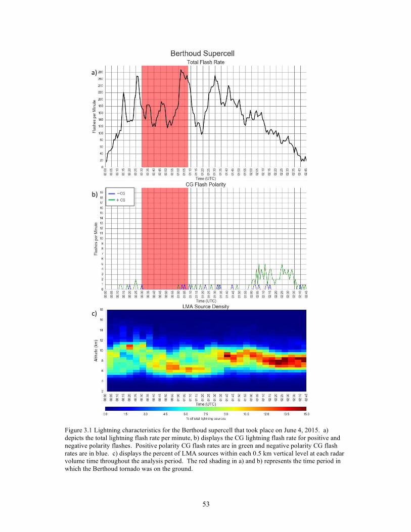
53

!

a)

b)

c)

Figure 3.1 Lightning characteristics for the Berthoud supercell that took place on June 4, 2015. a)

depicts the total lightning flash rate per minute, b) displays the CG lightning flash rate for positive and

negative polarity flashes. Positive polarity CG flash rates are in green and negative polarity CG flash

rates are in blue. c) displays the percent of LMA sources within each 0.5 km vertical level at each radar

volume time throughout the analysis period. The red shading in a) and b) represents the time period in

which the Berthoud tornado was on the ground.

!!!!!!−CG#

#### +!CG#

54

!

!!!!!!!!!!!!!

b)

a)

Figure 3.2 Visible imagery over the Berthoud supercell and surrounding storms. The white

box outlines the region where the overshooting top is visible for the Berthoud supercell. a)

shows well defined shadows and a cauliflower like texture at 00:09:00 UTC while b) shows

no such structure at 00:25:00 UTC.

00:09:00#UTC

00:25:00#UTC

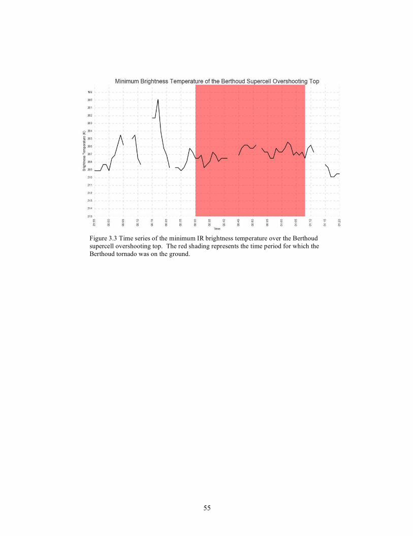
55

Figure 3.3 Time series of the minimum IR brightness temperature over the Berthoud

supercell overshooting top. The red shading represents the time period for which the

Berthoud tornado was on the ground.

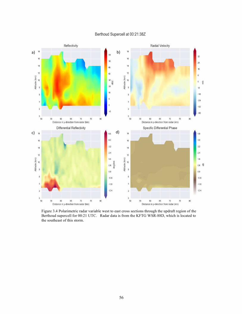
56

Figure 3.4 Polarimetric radar variable west to east cross sections through the updraft region of the

Berthoud supercell for 00:21 UTC. Radar data is from the KFTG WSR-88D, which is located to

the southeast of this storm.

a)

c)

b)

d)

57

b)

a)

Figure 3.5 Hydrometeor characteristics for the Berthoud supercell. a) represents the

mean conditional rain rate throughout the duration of the analysis period with a value

calculated for each radar volume time. b) displays the graupel mass (dotted blue line),

graupel volume (solid blue line), hail mass (dotted green line), and hail volume (solid

green line) found above the freezing level throughout the duration of the storm over

time. Red shading represents the time period in which the Berthoud tornado was on the

ground.

58

Figure 3.6 Same as 3.4, but for the updraft region of the Berthoud supercell at 00:43:24 UTC.

c)

a) b)

d)

59

Figure 3.7 Same as 3.1 but for the Denver supercell that took place on May 21, 2014.

a)

b)

c)

!!!!!!−!CG

###### +!CG

!

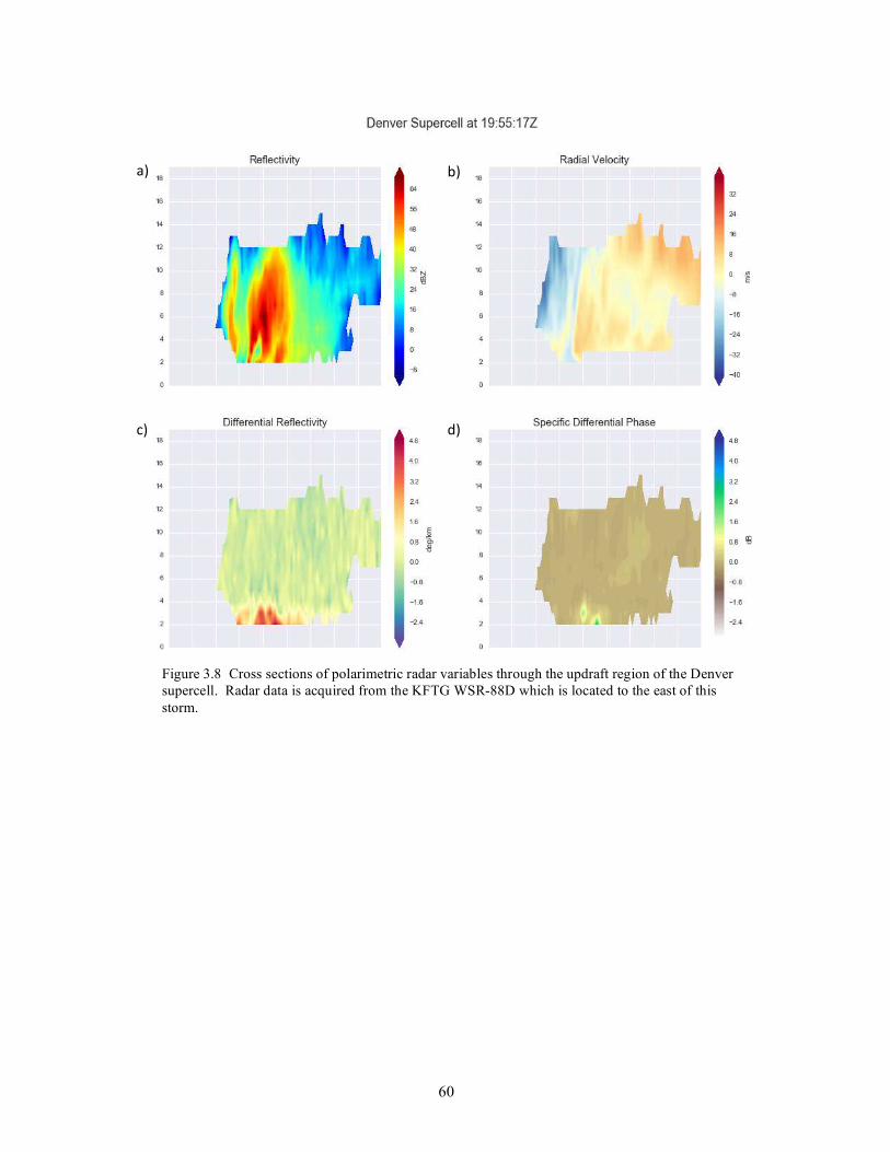
60

Figure 3.8 Cross sections of polarimetric radar variables through the updraft region of the Denver

supercell. Radar data is acquired from the KFTG WSR-88D which is located to the east of this

storm.

a)

c)

b)

d)

61

Figure 3.9 RHI of updraft region in the Denver supercell for 20:25 UTC. Polarimetric radar data

acquired by the CSU CHILL radar which is located to the north of this storm.

c)

c)

b)

d)

62

Figure 3.10 RHI of updraft region in the Denver supercell for 20:38 UTC. Polarimetric radar data acquired

by the CSU CHILL radar which is located to the north of this storm.

a)

c)

b)

d)

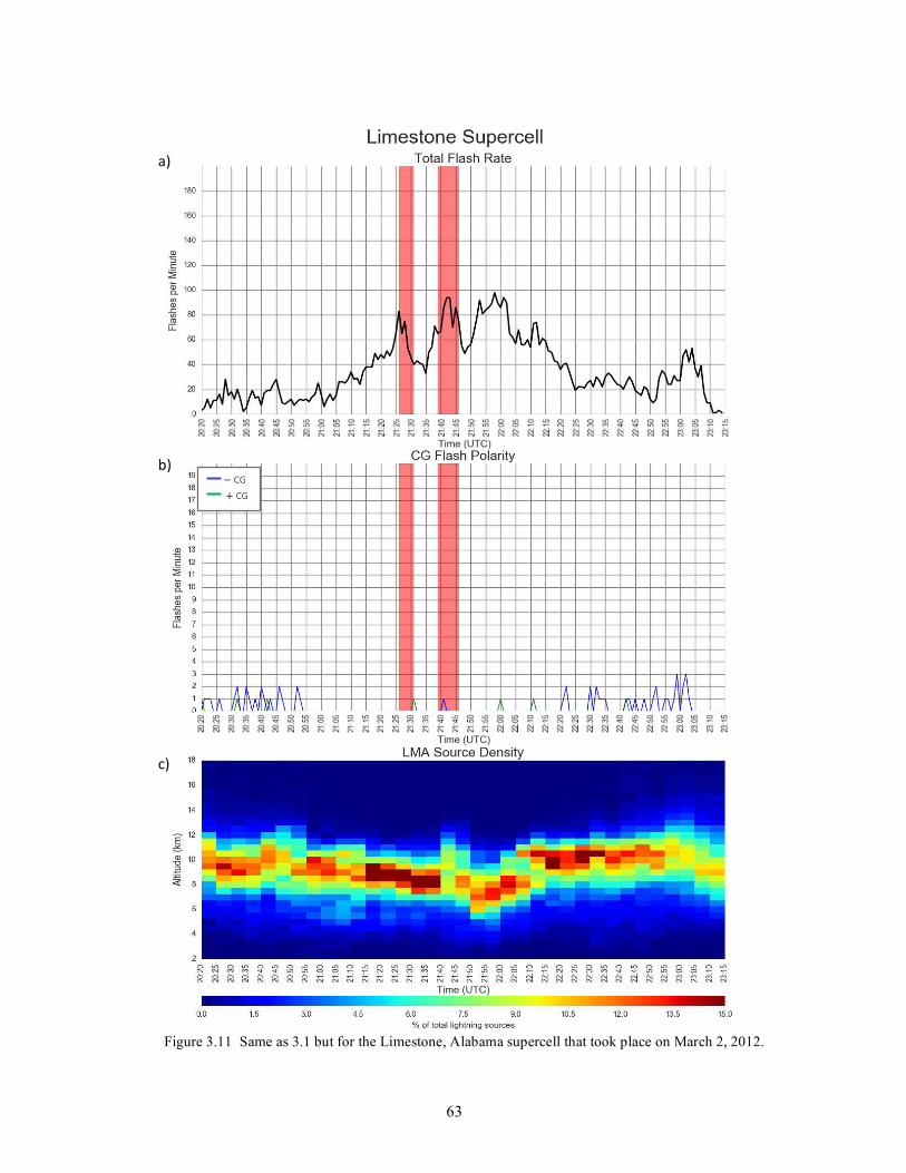
63

Figure 3.11 Same as 3.1 but for the Limestone, Alabama supercell that took place on March 2, 2012.

a)

b)

c)

!!!!!#−#CG ###### +!CG

64

Figure 3.12 Same as figure 3.5 but for the Limestone, Alabama supercell that took place on

March 2, 2012.

a)

b)

65

‘

Figure 3.13 Cross section of polarimetric radar variables along the updraft region of the

Limestone supercell for 21:16 UTC. Radar data shown is from the ARMOR radar. Arrows

represent the U/W wind vector created through dual Doppler analysis between the ARMOR

radar and KHTX WSR-88D.

a)

c)

b)

d)

66

Figure 3.14 Same as 3.13 but for the Limestone supercell at 21:19 UTC.

a) b)

c) d)

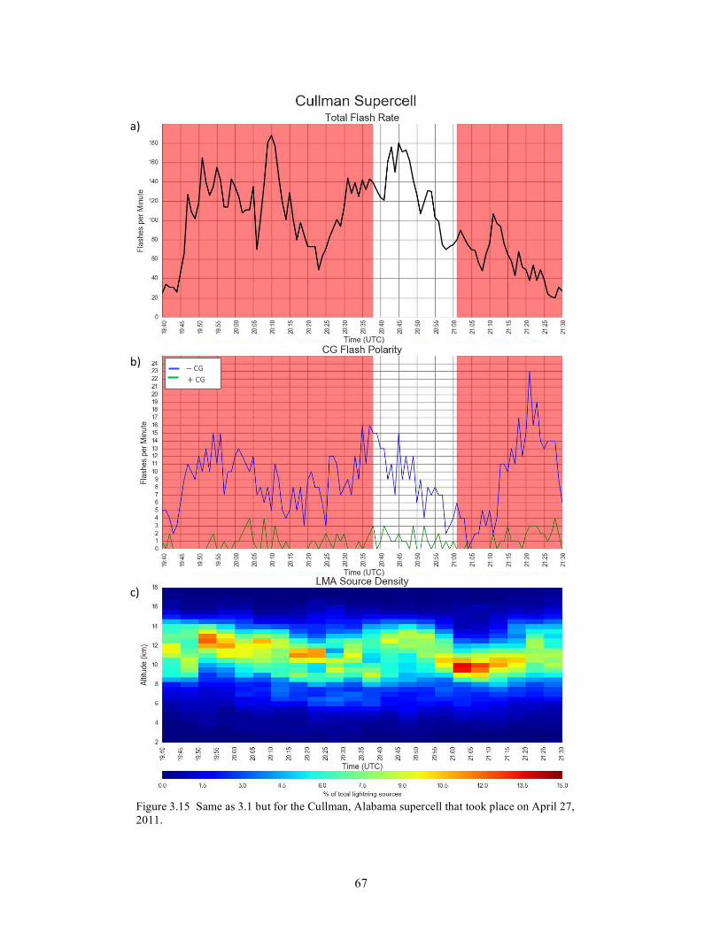
67

Figure 3.15 Same as 3.1 but for the Cullman, Alabama supercell that took place on April 27,

2011.

a)

b)

c)

!!!!!!−#CG ###### +!CG

68

Figure 3.16 Same as figure 3.5 but for the Cullman, Alabama supercell that took place on April

27, 2011.

a)

b)

69

Figure 3.17 Polarimetric radar variable cross sections through the updraft region of the Cullman,

Alabama supercell at 20:23 UTC. Polarimetric data displayed is from the ARMOR radar. Dual-

Doppler analysis was completed by using the ARMOR radar and the KHTX WSR-88D.

a) b)

c) d)

70

dB

Z

Figure 3.18 Low level PPI scan of the pre-storm environment before the Fort Lupton Landspout.

A fine-line can be seen in the boxed region of the reflectivity field in a). This fine line

corresponds to a region of convergence depicted in the radial velocity field in b).

a)

b)

71

Figure 3.19 Lightning characteristics for the landspout storm that occurred near Fort Lupton, CO on

July 28, 2014. a) depicts the total lightning flash rate for the time period in which this storm was

isolated from other nearby convection. b) displays the percent of LMA sources found at each 0.5 km

height interval in the Fort Lupton storm. Each column represents a radar volume. There were no

CG’s produced during the analysis period for this storm. Red shading represents the time period in

which a landspout was reported.

a)

b)

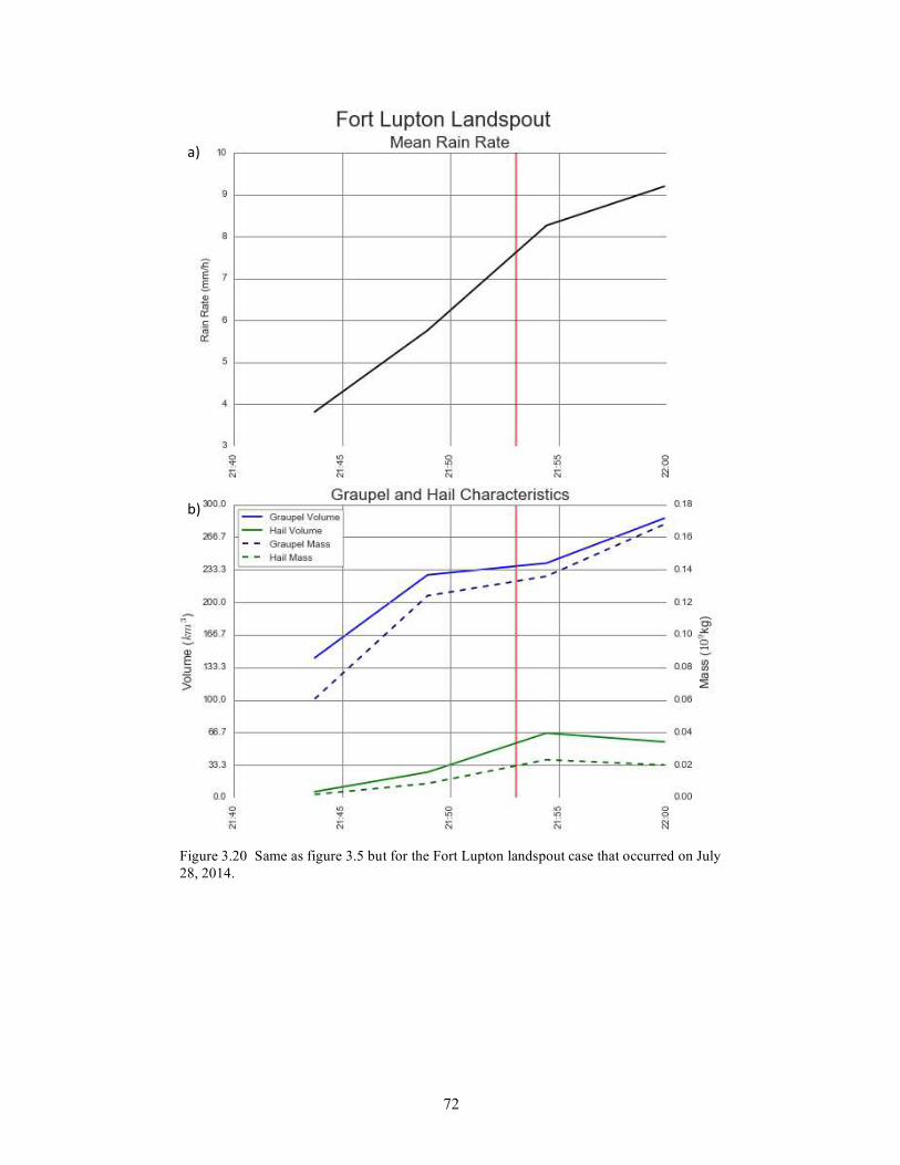
72

Figure 3.20 Same as figure 3.5 but for the Fort Lupton landspout case that occurred on July

28, 2014.

a)

b)

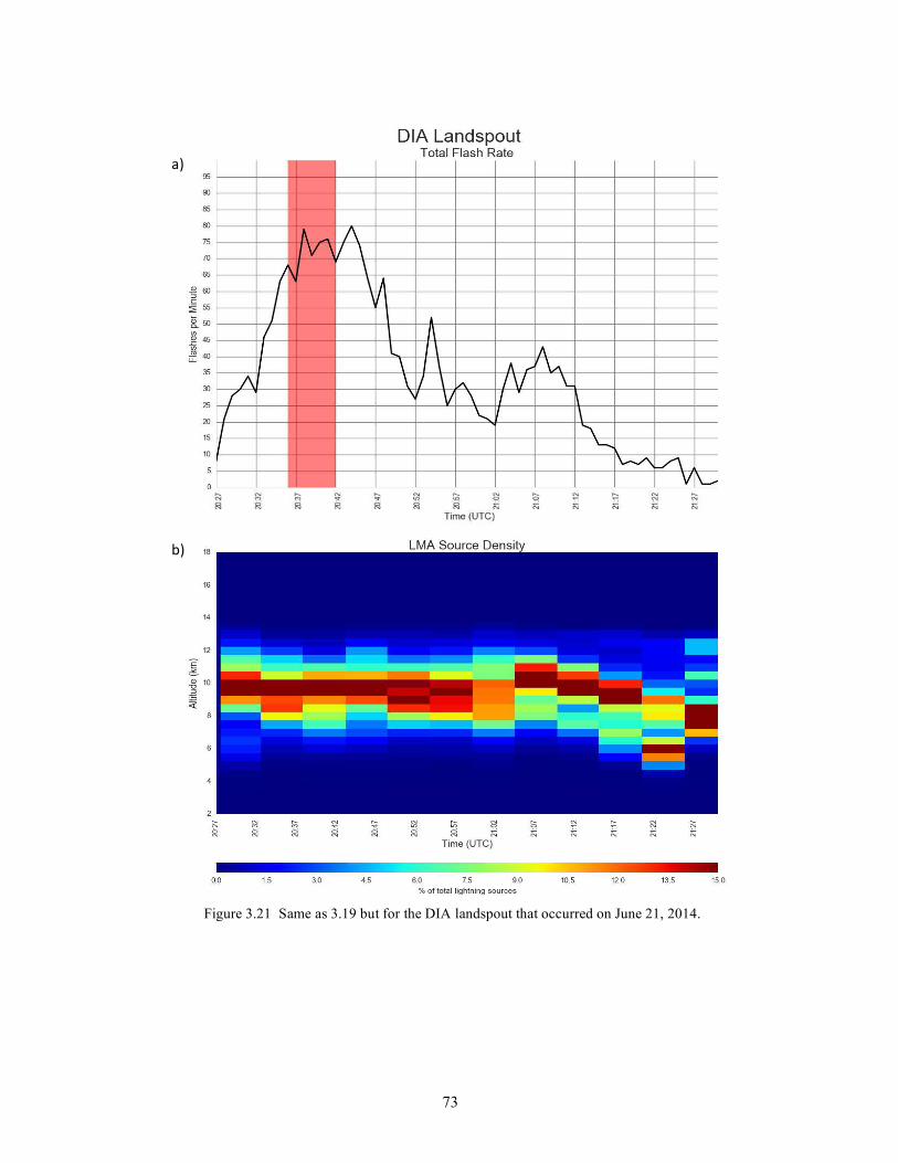
73

Figure 3.21 Same as 3.19 but for the DIA landspout that occurred on June 21, 2014.

a)

b)

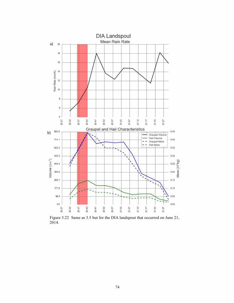
74

Figure 3.22 Same as 3.5 but for the DIA landspout that occurred on June 21,

2014.

a)

b)

75

CHAPTER 4: DISCUSSION AND CONCLUSIONS

4.1 LIGHTNING IN TORNADIC SUPERCELLS

Previous studies have found that the total lightning flash rate often “jumps” or increases

rapidly before the onset of severe weather (e.g. Williams et al. 1999; Goodman et al. 2005;

Schultz et al. 2009, 2011, 2015; Gatlin and Goodman 2010; Stano et al. 2014). The flash rate

increases as a result of an updraft intensifying as a storm strengthens and matures to the point

that it is able to produce severe weather. This relationship between severe weather and lightning

flash rate is useful in nowcasting situations when lightning data are available (Darden et al. 2010;

White et al. 2012). Soon, total lightning data will be available for the entire western hemisphere

thanks to the launch of the Geostationary Lighting Mapper (GLM; Goodman et al. 2013) on the

GOES-16 satellite. GLM will provide 60 s updated data continuously over the entire western

hemisphere. Improving our understanding of how all types of severe weather directly relate to

the evolution of lightning in a storm will help forecasters best utilize the new data provided by

GLM.

Supercellular tornadoes form in association with a mesocyclone within a mature

supercell. Analysis of the Berthoud and Denver storms in this thesis suggests that in scenarios

that multicellular convection organizes into a supercell, this organization may be accompanied

by a sharp rise in flash rate. The Denver supercell began as a cluster of thunderstorms with total

lightning flash rates near 20 flashes min-1

. The flash rates increased in conjunction with the

organization of these storms. A peak in flash rate occurred when a mesocyclone first became

evident within the Doppler radar radial velocity field. The Berthoud supercell showed the same

trait. In this case, the Berthoud supercell had weakened significantly during the touchdown of

76

the Berthoud tornado and lost its defined mesocyclone. The former supercell appeared to

maintain more of a multicellular structure. As the storm reorganized to maintain a defined

mesocyclone, the flash rates showed a rapid increase. This relationship corroborates other

studies (e.g. Darden et al. 2010; Stano et al. 2014) and could serve useful to forecasters in

determining which storm clusters will organize into more intense convection.

Charge separation that produces lightning results from the collision of graupel and ice

crystals in the presence of supercooled liquid water (e.g., Reynolds et al. 1957). Intensifying

updrafts lead to the formation of more graupel and ice crystals as more liquid water is made

available for riming growth. Should larger supercooled drops be lofted into the mixed phase

region, they rapidly freeze to become graupel particles. Intensifying updrafts also lead to more

turbulence, which may promote more collisions between falling graupel and rising ice crystals,

leading to more charge separation. These processes cause flash rates to increase as a

mesocyclone develops. However, this characteristic is not limited to the formation of a

mesocyclone. This analysis demonstrates that this process occurs any time that an updraft

intensifies sufficiently to produce ice and electrification, resulting in lightning flash rates

increasing regardless of the storm’s maturity.

As the updraft of the Berthoud supercell first intensifies before the onset of the tornado,

the flash rates increase rapidly from 20 flashes min-1

to nearly 270 flashes min-1

over a 25-minute

period. This prolific increase in total lightning flash rate is accompanied by increasing graupel

and hail volumes, a decreasing minimum brightness temperature over the overshooting top, and

an increase in the height of the VHF sources. The increase in graupel volume is consistent with

updraft intensification, as discussed above. The increase in updraft intensity also causes the

location of the VHF sources to rise with it, creating the increase in VHF source density heights.

77

Rising VHF sources do not appear each time an updraft intensifies. The Berthoud storm

displays other periods of intensifying updrafts that correspond to rises in total lightning flash rate

and increases in graupel volume, but these time periods do not show an increase in the VHF

source density height. For example, just before the Berthoud tornado lifts, the total lightning

flash rate of the Berthoud supercell increases rapidly. The VHF sources show no strong upward

ascent. They appear to “spread out” such that the sources are not highly concentrated at a

specific elevation. This likely occurs because updraft intensification promotes enhanced

turbulence which helps to create smaller pockets of charge along the periphery of the updraft.

More frequent, smaller flashes occur causing the VHF sources to appear throughout the

atmospheric column (Bruning and MacGorman 2013).

Similar to the beginning stages of the Berthoud supercell, the Denver storm shows an

initial rise in the VHF sources in conjunction with increasing flash rates as the storm first

develops, prior to the touchdown of the first tornado. There is a spreading out of the source

densities as the flash rates recover after dropping significantly during the onset of the first

tornado, but any other increase in flash rate is not accompanied by significant changes in the

VHF source densities. The Cullman case on the other hand, shows VHF sources varying in

height with the changes in the total lightning flash rate. Increases in flash rate are accompanied

by increases in VHF source heights, while decreases in flash rate are accompanied by the descent

of VHF source heights. The Limestone case did not display this relationship. The first increase

in flash rate that occurs prior to the formation of the first tornado shows no change in the source

density heights. The VHF sources remain confined to a relatively thin layer through the duration

of the storm. There is a slight spreading out of the VHF sources with height as the flash rate

increases during the onset of the second tornado.

78

In each supercell analyzed, the flash rate consistently increases during radar indicated

periods of updraft intensification, consistent with the relationship between intensifying updrafts

and increasing flash rates found in past studies. Steiger et al. (2005, 2007) found that when

storms were most intense, lightning occurred at the highest altitudes during the storm’s history.

This study shows that this is not always true. The Denver and Berthoud supercells show an

increase in the source density height as the storm develops, but the VHF sources do not vary

during re-intensification of the storms. The Cullman supercell tends to support Steiger et al.

(2005, 2007) as the VHF source rise and fall with increasing flash rates and thus intensifying

updrafts. The Limestone supercell is unique in that the source heights decrease as the storm

intensifies. The storm reverses polarity from normal to anomalous, perhaps associated with

higher amounts of supercooled water aloft, thereby promoting positive charge on graupel.

Though the evolution of these storms do not fully support the findings in Steiger et al., it is

interesting to note that the Cullman storm, which produced the highest echo top heights and most

severe tornado, displayed VHF sources well above 10 km. The other cases showed VHF sources

remaining near 10 km.

Multiple studies have indicated that the total lightning flash rate typically decreases

during the onset of a tornado (Williams et al. 1999; Steiger et al. 2005, 2007; White et al. 2012).

These studies agree that this decrease in flash rate is likely a result of the updraft weakening and

a downdraft forming since supercellular tornadoes require a downdraft to advect vertical

vorticity to the surface where it can be stretched by the updraft. Steiger et al. (2005, 2007)

suggests that lightning decreases in height as downdrafts form before tornadogenesis. This study

supports this notion along with the idea that flash rates decrease during tornadogenesis. The

Berthoud tornado is an ideal example. Just prior to the onset of the tornado, the flash rates

79

decrease sharply and there is a descent of the VHF source densities throughout the duration of

the tornado. Decreasing graupel volume in conjunction with increasing rain rates are consistent

with the formation of a downdraft.

The Denver supercell shows an extreme decrease in flash rate prior to the onset of the

first tornado. The VHF sources begin to decrease in height only after the tornado is on the

ground. The VHF sources show no definitive trend once the second and third tornado form, but

there is an apparent rise in flash rate and then decrease prior to the onset of both of these

tornadoes. Only a portion of the Cullman supercell could be analyzed, but the onset of the

second tornado also supports the notion that lightning data is suggesting downdraft formation.

The second tornado in the analysis touches down while the flash rates are decreasing. There is

also a descent in the source densities as tornadogenesis begins. The first Cullman tornado begins

before the analysis time, so information was not attained about the flash rates and its initial

formation.

The Limestone supercell shows slightly different trends when it comes to total lightning

flash rates and VHF source heights. The first tornado reported within the analysis period touches

down right as the peak in flash rate is reached. The second tornado occurs while the flash rates

increase to a peak and then begin to fall. The VHF sources show a very gradual descent during

the period of tornadogenesis, but the descent is not significant enough to discern any obvious

trend. Evidence of a downdraft occurs as graupel volume decreases and rain rate increases

throughout the duration of tornadogenesis, but the flash rate does not follow the trends found in

the other three supercellular cases. Part of this may be due to error in spotter-reported times in

which a tornado was on the ground.

80

Though the Limestone supercell shows differing trends, it is noteworthy that three of the

four cases analyzed depict signs of downdraft formation within the lightning data. Awareness of

these trends could serve useful to forecasters during nowcasting situations. It is interesting to

note that the trends in flash information were not as robust during secondary tornadogenesis

during the Denver supercell. This is likely a result of the fact that secondary tornadogenesis is

easier to achieve because the environment left behind by original tornadogenesis supports the

formation of horizontal vorticity that can be tilted vertically, and subsequently advected to the

surface and stretched to form subsequent tornadoes (Davies-Jones et al. 2001).

Decreases in graupel volume also were found to coincide with the formation of a

downdraft, which may serve useful to forecasters if sufficient radar data along with HID

information is available. Using graupel volume calculations in conjunction with total lightning

flash rates would provide forecasters with valuable information that could be used to predict the

formation of a downdraft. Analysis completed in this thesis suggest that rises and falls in

graupel volume are less abrupt than rises and falls in the minute by minute flash rate. Graupel

volumes also tend to display a less noisy curve. As a result, this analysis shows that a decrease

in graupel volume above the freezing level may be a more reliable way of determining when a

downdraft forms. Ideally, witnessing a decrease in graupel volume at the same time as a

decrease in lightning flash rate would be the most reliable way of determining downdraft

formation. Radar data is not always available to forecasters due to power outages or blockage

from high terrain. With the launch of GOES-16 and the availability of total lightning data from

GLM, it is important to define relationships between lightning information and storm dynamics

as GLM will continually provide lightning coverage in areas that may not have access to weather

radars.

81

No trend in the production of CG flashes during tornadogenesis is indicated in this study.

The apparent lack of relationship between tornado formation and CG production has been well

reported in the literature (Perez et al. 1997; MacGorman et al. 1989; Keighton et al. 1991;

MacGorman and Nielsen 1991, Strader and Ashley 2014). Both the Denver and Berthoud

supercells show the formation of an EOSO at the end of their lifetime. The Berthoud supercell

displays a decrease in flash rate and a decrease in VHF source density heights as the number of

+CG’s quickly increases. The Denver supercell does not show a decrease in flash rate, but there

is a descent in the VHF source heights as the +CG rate increases substantially. The EOSO in

both of these cases is linked to the fallout of precipitation-sized ice particles, as indicated by

radar cross sections. The Berthoud case also shows a decrease in the graupel volume, most

likely resulting from graupel fallout. As the graupel falls through the cloud, negatively charged

hydrometeors fall out of the cloud, leaving behind a large amount of positively charged

hydrometeors that fall closer to the surface (indicated by the descent in VHF sources). This

descent in the positive charge layer likely promotes the formation of +CG flashes.

An interesting final note about this analysis is the difference between the Alabama and

Colorado supercells. Colorado is located in the High Plains region which is characterized by

high cloud base heights in a relatively dry, warm environment. High cloud base heights promote

the formation of broad updrafts as parcels have more time to expand as they move upward.

These high cloud base heights result in small warm cloud depths, which promote enhanced ice

formation in the reduction of robust warm rain processes. These traits are clearly indicated in

comparisons of graupel volume. Increases in graupel volume indicate enhanced graupel

production. Graupel production in the Colorado cases is significantly larger than the Alabama

cases. This enhanced graupel production corresponds to larger flash rates in the Colorado storms

82

overall as well. Regardless of these differences, the lightning trends are similar in both locations,

suggesting that information that can be gained from lighting trends holds constant across varying

environmental backgrounds.

4.2 LIGHTNING IN LANDSPOUTS

Two case studies of landspouts completed over the Colorado region depict identical

lightning characteristics during the materialization of a landspout at the surface. As discussed in

Chapter 1, landspouts form differently than supercellular tornadoes. They do not require a

downdraft to form. Rather, they require vertical vorticity to already be present at the surface.

When an updraft of a developing storm moves over a region of enhanced surface vertical

vorticity, the vorticity is stretched and advected towards the inflow region, creating enhanced

vertical vorticity throughout the atmospheric column (Wakimoto and Wilson 1989). This

enhanced vorticity can lead to the formation of a landspout.

In both the DIA and Fort Lupton landspout, the flash rate is increasing when the

landspout touches down. The increasing flash rate is consistent with the idea that landspouts

form as updrafts move over a region of vertical vorticity and intensify. The graupel and hail

volume are both increasing during the onset of the landspout, further supporting the idea that the

updraft is intensifying. Graupel volumes are significantly larger than the hail volume for both of

these cases. These storms also produce a significantly smaller number of flashes compared to

the Colorado supercells described above. This is likely a result of these storms being weaker and

shorter lived. The VHF sources remain confined to a small area in the storm due to presumably

weaker updrafts being unable to loft hydrometeors to the same altitudes as supercellular updrafts.

The smaller flash rates also lead to less production of VHF sources, resulting in defined regions

of VHF source density.

83

The Fort Lupton storm merged with other convection before its dissipation could be

observed. In the DIA landspout storm, the landspout lifts just prior to the peak in flash rates.

The flash rates then decrease steadily as graupel and hail volumes decrease and rain rates remain

large. Landspouts are sustained by updrafts, so weakening of the updraft due to precipitation

loading likely led to the landspout’s demise. Forecasters may find utility in monitoring storms

for increasing flash rates when they are aware of vertical vorticity already being present at the

surface, such as by the presence of a DVCZ. Monitoring storm intensification in such situations

through monitoring flash rates could serve useful in determining which storms could potentially

produce landspouts that day.

84

CHAPTER 5: SUMMARY

Overall, this study has demonstrated that lightning data can reveal information about the

dynamics within a tornadic storm. Updraft intensification is accompanied by increases in total

lightning flash rate, and sometimes an increase in the VHF source heights. The organization of a

cluster of thunderstorms into a supercell is also characterized by increasing total lightning flash

rates and increasing VHF source heights. Tornadogenesis in supercells is typically characterized

by decreasing flash rates and descending VHF source densities. This descent likely occurs as a

result of updraft weakening and downdraft formation. This idea is supported by indications of

decreasing graupel volume and increasing rain rates during the majority of the tornado

touchdowns analyzed. Downdrafts are necessary for supercellular tornado formation because

they advect vertical vorticity to the inflow region of the storm, where the vorticity can be

stretched to create enhanced vertical vorticity at the surface. It is logical that the formation of

these downdrafts would be evident in lightning characteristics since lightning flash rates are

heavily dependent on the strength of an updraft.

Landspout storms do not require the formation of a downdraft, rather they are

characterized by updrafts intensifying over regions of already present vertical vorticity.

Landspouts analyzed in this study are characterized by increasing flash rates. The tornadoes lift

before flash rates begin to decrease. Understanding how flash rates and other lightning

characteristics relate to the formation of tornadoes is important for nowcasting purposes.

Knowing that landspouts form during increases in flash rate could help forecasters focus their

energy on individual storms showing signs of intensification in regions where vertical vorticity is

already present. Forecasters can also find use in knowing that lightning information can

85

sometimes point towards the formation of a downdraft, supporting supercellular tornado

formation. Increasing total lightning flash rates with increasing updraft strength is also a very

useful relationship as intensifying updrafts can lead to any type of severe weather.

More case studies need to be completed to develop a more robust understanding of how

lightning can be used to diagnose dynamic evolution within potentially tornadic storms, but it is

promising to see trends within such a small number of cases. With the imminent release of GLM

data to atmospheric scientists, larger scale studies can be completed to assist in this effort as

lighting data will be available for the entire western hemisphere.

86

CHAPTER 6: THE GEOSTATIONARY LIGHTING MAPPER

6.1 INTRODUCTION

The Geostationary Lightning Mapper (GLM) is the first instrument to detect lightning

from the geostationary orbit. GLM was created to assist forecasters in nowcasting severe

weather situations and in detecting regions where lightning is located, with an emphasis on total

lightning detection and more detailed description of lightning outside of surface networks.

Eventually, GLM will also provide researchers with a long term climatological database for

lightning information (Goodman et al. 2013). Onboard GOES-16, launched in November of

2016, the GLM is currently in its calibration/validation stages in preparation for operational

commission. The calibration/validation process has involved a field campaign whose goal was to

target storms occurring in regions that have VHF-based Lightning Mapping Arrays (LMAs).

The campaign aimed to assess the GLM flash detection efficiency in various types of storms by

comparing GLM flash detections to flash detections made by other instruments, including

LMAs.

As part of these calibration/validation activities, we participated in the 8 May 2017 flight

campaign mission that targeted the Colorado LMA on a fortuitously severe weather day. During

this mission, the NASA ER-2 flew over many strong hail producing storms, collecting data with

the Fly's Eye GLM Simulator (FEGS) and numerous other sensors from 22:00 to 01:00 UTC.

This instrument detects lightning in the same way that GLM does, but at a smaller capacity since

it is only able to the see regions overflown by the NASA-ER2. The CSU-CHILL radar was

operated on this day to provide high quality polarimetric and Doppler observations of

convection. Sector scans were performed over storms targeted by the ER-2. PPI sector scans

87

topped the storms such that the anvil region could also be observed and eventually compared to

information gained from the Advanced Baseline Imager (ABI; Schmit et al. 2005) also on board

of GOES-16. High resolution RHI scans were taken to display the complex structure and

strength of each targeted storm.

Data collected by FEGS onboard the NASA ER-2 and data collected from CSU-CHILL

provide ample data sources to scientists analyzing the initial results of the GLM instrument.

LMA data, NLDN data, as well as Earth Networks Total Lightning Network (ENTLN) data were

recorded and are available for analysis as well. To understand how well GLM performs in

various types of intense storms, this study takes a “deep dive” look at three individual storms

during field campaign operations on 8 May 2017. By analyzing GLM data and comparing it to

other forms of lightning information on a storm cell basis, changes in GLM flash detection

efficiency can be directly related to changes in other parameters within a storm.

6.2 DATA

6.2.1 GEOSTATIONARY LIGHTNING MAPPER

The GLM detects optical emissions produced by lightning that emerge at the top and/or

sides of clouds (depending on satellite viewing geometry). Characterized by a 1372 x 1300 pixel

Charge Coupled Device (CCD) focal array, the spatial resolution of the GLM is 8 km at nadir

expanding to 14 km at the edge of the field of view (Goodman et al. 2013). Product latency is

less than 20 seconds. Various filtering techniques are utilized to filter out unwanted light so that

lightning can be seen even during broad daylight when cloud tops may appear brighter than the

emissions produced by lightning. Four unique filters are used on board the space-craft before

ground processing further refines the data (Goodman et al. 2012).

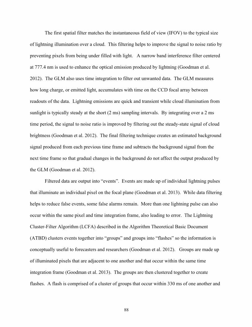
88

The first spatial filter matches the instantaneous field of view (IFOV) to the typical size

of lightning illumination over a cloud. This filtering helps to improve the signal to noise ratio by

preventing pixels from being under filled with light. A narrow band interference filter centered

at 777.4 nm is used to enhance the optical emission produced by lightning (Goodman et al.

2012). The GLM also uses time integration to filter out unwanted data. The GLM measures

how long charge, or emitted light, accumulates with time on the CCD focal array between

readouts of the data. Lightning emissions are quick and transient while cloud illumination from

sunlight is typically steady at the short (2 ms) sampling intervals. By integrating over a 2 ms

time period, the signal to noise ratio is improved by filtering out the steady-state signal of cloud

brightness (Goodman et al. 2012). The final filtering technique creates an estimated background

signal produced from each previous time frame and subtracts the background signal from the

next time frame so that gradual changes in the background do not affect the output produced by

the GLM (Goodman et al. 2012).

Filtered data are output into “events”. Events are made up of individual lightning pulses

that illuminate an individual pixel on the focal plane (Goodman et al. 2013). While data filtering

helps to reduce false events, some false alarms remain. More than one lightning pulse can also

occur within the same pixel and time integration frame, also leading to error. The Lightning

Cluster-Filter Algorithm (LCFA) described in the Algorithm Theoretical Basic Document

(ATBD) clusters events together into “groups” and groups into “flashes” so the information is

conceptually useful to forecasters and researchers (Goodman et al. 2012). Groups are made up

of illuminated pixels that are adjacent to one another and that occur within the same time

integration frame (Goodman et al. 2013). The groups are then clustered together to create

flashes. A flash is comprised of a cluster of groups that occur within 330 ms of one another and

89

are separated by no more than 16.5 km spatially (Goodman et al. 2013). A flash can be made up

of many events and groups, or it can be made up of one event and group. An example of this

grouping is shown in Figure 6.1. The ATBD also mentions that there is potential for multiple

flashes to be labeled as one flash due to the generous temporal and spatial thresholds used to

define a flash, compared to the finer space/time scales upon which lightning pulses actually

occur.

6.2.2 LIGHTNING MAPPING ARRAY

An LMA detects electromagnetic radiation emitted by lightning at frequencies between

60-66 MHz (Rison et al. 1999, Krehbiel et al. 2000). LMAs use GPS time of arrival techniques

to geolocate burst radiation from lightning discharges. These sources of radiation can be

grouped into flashes utilizing a flash clustering algorithm described in Fuchs et al. (2015) and

summarized in Chapter 2. The flash clustering algorithm uses spatial and temporal thresholds

based on physical expectations of lightning size and duration, to cluster sources into flashes.

Typically for the Colorado LMA, thresholds are set such that sources within a specific flash

cannot be separated by more than 3 km and be no more than 150 ms apart in time. For this

study, these values are expanded to more generous terms to account for the generous thresholds

set for GLM flash clustering. Accordingly, the temporal and spatial thresholds are set to 330 ms

and 16.5 km respectively.

6.2.3 NATIONAL LIGHTNING DETECTION NETWORK

The NLDN detects radiation emitted by lightning in the VLF (3-30 kHz)/LF (30-300

kHz), which is much different than the range of frequencies utilized for the LMA (Cummins et

al. 1998; Cummins and Murphy 2009). Lower frequencies do not detect the small flashes that

are typically seen by the LMA, including IC flashes. Rather, they are very good at detecting

90

large CG flashes and longer IC flashes. For this reason, NLDN data were used solely for

detecting CG flashes and their corresponding polarity throughout this study. IC and CG flashes

are differentiated through analysis of the waveform of the radiation recorded. Sometimes this

analysis erroneously classifies IC as CG flashes. To ensure that CG flashes used in this study are

truly CG flashes, all flashes classified as CG that recorded peak currents smaller than 15 kA

were reclassified as IC flashes, and therefore excluded from analysis. If an IC flash created a

peak current larger than 25 kA, then the flash was recorded as CG (recommendations per

personal communication with Dr. Timothy Lang).

6.2.4 EARTH NETWORKS TOTAL LIGHTNING NETWORK

Earth Networks Total Lightning Network (ENTLN) detects radiation emitted by lightning

at frequencies ranging from 1 Hz to 12 MHz (Liu and Heckman 2011). This network uses time

of arrival techniques to locate pulses of lightning and then groups the pulses into flashes.

ENTLN is a near global network that detects both IC and CG flashes across many countries.

ENTLN sensors are separated by hundreds of kilometers, causing their accuracy in detecting the

altitude of a flash to be poor compared to an LMA (Liu and Heckman 2011). For the sake of this

study, only the latitude and longitude location and time of an ENTLN flash is used in comparing

the flashes observed by different systems.

6.2.5 NATIONAL MOSAIC AND MULTI-SENSOR QPE SYSTEM

The National Mosaic and Multi-Sensor Quantitative Precipitation Estimate System

(NMQ) ingests level 2 base data from the NWS WSR-88D’s as well as the Canadian weather

radar network and grids the reflectivity field to a 3-dimensional Cartesian grid such that radar

information for the entire CONUS domain is visible on a single display. This system also uses

multiple sensor systems such as radar and rain gauges to produce a quantitative precipitation

91

estimate that is useful for flash flood forecasting. This study utilizes the 3-dimensional gridded

reflectivity field to analyze the storms targeted during the 8 May 2017 field campaign mission.

Many of the storms from this day occurred along the edge of the KFTG WSR-88D range. By

using NMQ data instead of information from one WSR-88D, gaps in storm coverage are

avoided.

6.3 ANALYSIS METHODS

6.3.1 CLEAR

The CSU Lightning, Environment, Aerosol, and Radar (CLEAR; Lang and Rutledge

2011) framework was implemented to track the storms targeted on 8 May 2017. Due to these

storms passing directly over the cone of silence of the CSU-CHILL radar, NMQ radar data was

used instead. As described in Chapter 2, CLEAR uses reflectivity and spatial thresholds to

identify convective features and track them over time. For this study, storms were required to

have a 35 dBZ contour at least 20 km2 in area as well as a 45 dBZ contour of at least 10 km

2 in

area to be identified as a convective entity.

6.3.2 FLASH ATTRIBUTION

The flash clustering algorithm mentioned above, fully explained in Fuchs et al. (2015),

also attributes individual flashes to storm cells defined by the CLEAR framework. In this study,

LMA, ENTLN, and NLDN flashes are attributed to each identified storm cell. Flashes that occur

within the storm cell 35 dBZ contour or within 10 km of the storm cell are attributed to the

storm. GLM flashes, sources, and events are also attributed to each storm. If a GLM flash

occurs within the storm cell or within 15 km of the storm cell, the flash is attributed. The GLM

attribution parameter is slightly more generous than those defined for the other lighting networks

due to known errors in the non-operational GLM flash locations. The generous attribution

92

parameter may cause a few flashes from other storms to be attributed to the storms of interest,

but analysis periods were chosen for time periods in which the storms remained relatively

isolated for this reason.

6.3.3 LIGHTNING ANALYSIS

The main objective of this study is to compare the flash rates produced by LMA and

ENTLN networks to those produced by the GLM to determine how well the GLM is performing

in its preliminary stages. Flash rates are determined by binning cell attributed flashes of a storm

of interest into one minute intervals and counting the number of flashes in each bin. This

methodology is applied in determining the minute by minute GLM event and group counts, as

well as the CG flash polarity counts. To determine how well GLM detects lightning compared to

high resolution information gained by LMAs, the GLM/LMA ratio is determined by dividing

each GLM flash rate count by the LMA flash rate that corresponds to the same time interval. By

doing so, a GLM detection efficiency is created with LMA flashes (the latter considered as

truth).

In an effort to understand why GLM detection efficiencies fluctuate throughout a storm’s

lifetime, the flash areas and flash altitudes recorded in the LMA data are further analyzed.

Because LMAs detect individual sources of radiation emitted by lightning, LMA data reveals

flash information in 3 dimensions. The flash area is determined by projecting the sources of a

flash onto a 2D plane and then creating a convex hull around the outer points of the flash

(Bruning and MacGorman 2013). The area within the convex hull is defined as the flash area. A

visualization of this idea is found in Figure 6.2. The flash altitude is taken as the altitude of the

flash centroid. The median flash altitude and flash area for each radar volume time span is

recorded and displayed in a time series to depict how the flash areas and altitudes vary with time.

93

The median value was chosen instead of the mean so that outlying points did not skew the

results.

6.4 RESULTS AND DISCUSSION

6.4.1 FORT MORGAN NORMAL POLARITY STORM

Figure 6.3 displays the lightning characteristics for a one-hour period of a storm observed

by the NASA ER-2 on 8 May 2017. This storm was long lived, forming before the field

campaign mission started and dissipating after the NASA ER-2 began its return to base. The

analysis period of this storm was chosen because during this period the storm remained isolated

from other convection. Choosing time periods in which convection is isolated ensures flashes

attributed to a storm are not influenced by other lightning producing convection. Figure 6.3a

indicates that the LMA produced flash rates significantly larger than any other lightning

detecting system (Earth-based networks and GLM). ENTLN derived flash rates were over a

factor of two less than LMA. GLM flash rates were lower yet. The LMA displayed a peak in

flash rate near 210 flashes min-1

at about 23:12 UTC. Both ENTLN and the GLM show a rise

and fall in flash rate similar to the LMA, but their peaks occur at significantly different times and

the peaks are substantially less than LMA. ENTLN flash rates peak around 85 flashes min-1

at

23:07 UTC and the GLM flash rates peak at about 55 flashes min-1

at 23:16 UTC.

The GLM/LMA flash rate ratio is also displayed in Figure 6.3a to emphasize the time

periods in which the GLM detection efficiency with respect to LMA flashes was largest. The

ratio averages around 0.2. The highest detection efficiency occurs at 23:16 UTC when the GLM

flash rate peaks, reaching a detection efficiency of 31%. Figure 6.3b shows the GLM event rates

and group rates for this analysis period. The events and groups follow a similar trend to the

GLM flash rates, but produce much larger values. It is interesting to note that the GLM events

94

and groups follow the LMA flash rates more closely than the GLM flash rate itself. At the

beginning of the time period and the end of the time period, significantly more events and groups

are produced than LMA flashes, but from 22:57 to 23:12 UTC the GLM groups and events

follow the LMA flash rate trend and values rather closely.

Figure 6.3c displays the density of LMA sources binned by height throughout the

analysis period. There are two distinct altitudes of enhanced source density throughout the

analysis period. One maximum occurs between 10 and 12 km in altitude while the other occurs

between 4 and 6 km in altitude. This bimodal source structure is a classic signature that the

storm maintained a normal polarity charge structure. Electrical breakdown in a region of

positive charge produces more VHF radiation compared to positive break down within negative

charge, marking the location of positive charge by enhanced VHF sources. Since a normal tripole

charge structure is characterized by a negative charge layer sandwiched between an upper and

lower positive charge layer, a bimodal source density structure would suggest that a normal

tripole charge structure is present during this time period. This idea is confirmed in Figure 6.3d.

The storm produced predominantly negative CG’s throughout the entire analysis period.

Analysis of Figure 6.4a and Figure 6.4b show that the GLM/LMA ratio is increasing as

the median flash altitude and median flash area are both increasing at approximately 23:14 UTC.

It appears that a combination of larger flash areas and higher flash heights may lead to better

detection of lightning by GLM. Larger flashes have the opportunity to illuminate more GLM

pixels, making these flashes likely easier for GLM to detect. In theory, flashes that occur at

higher altitudes would be subject to less scattering and attenuation of optical emissions since

light produced by lightning must penetrate surrounding ice to reach the cloud tops. It is logical

that detection efficiencies should increase as the flash altitude increases, resulting from a smaller

95

amount of ice being present between a lightning flash and the top of the cloud. Analysis of the

ice water path between flashes and the cloud top would be a useful parameter to explore this idea

and should be pursued in future analysis.

Figure 6.4c shows that this storm consistently maintained reflectivity values of 55 dBZ.

The maximum echo heights do not appear to have a strong correlation with the GLM/LMA flash

ratio, but it is interesting to note that the slight rise in echo heights from 23:03 to 23:06 UTC

corresponds to a period of increasing flash rates in each of the lightning detecting networks.

Rising echo heights typically correspond to a strengthening updraft leading to the formation of

more ice particles. This strengthening updraft likely caused the flash rates to increase and the

flash size to decrease (Bruning and MacGorman 2013). During this period, the event and group

rates closely follow the LMA flash rates and the LMA flash areas are small compared to the rest

of the analysis period. Before and after this time period, the event and group rates are

significantly larger than the LMA flash rates and the LMA displays median flash areas that are

larger than those found from 22:57 to 23:12 UTC. This trend indicates that GLM events and

groups are clustered together into spatially large flashes as the LMA-inferred flash area gets

larger, as would be expected if the GLM clustering algorithm is performing well. When flashes

are small they likely only take up one pixel, causing the events and group rates to be similar to

one another and similar to the LMA flash rates.

6.4.2 GREELEY ANOMALOUS POLARITY CASE

A hail producing storm formed prior to the NASA ER-2 flight and persisted throughout

the mission time period. This hail producing storm passed directly over the CSU-CHILL radar

and produced a great deal of hail and rain in the process. The analysis period begins at the

beginning of the ER-2 mission (22:00 UTC) and continues until about 23:00 UTC. The analysis

96

terminates at this point because this Greeley storm began to merge with other convection. Figure

6.5a displays the flash rates determined by each lightning detecting network or instrument for

this storm. The LMA shows clearly defined increases and decreases in flash rate with flash rates

reaching nearly 300 flashes min-1

. ENTLN displays much smaller flash rates, with values

reaching only 65 flashes min-1

. The ENTLN flash rate trends are also very different from those

displayed by the LMA. ENTLN flash rates gradually decrease for the first half of the analysis

period and then remain relatively constant. GLM shows flash rates only reaching 30 flash min-1

with no definitive trend, unlike LMA. Because GLM does not show any definitive trends in

flash rate, the GLM/LMA ratio maximizes when the LMA flash rates are smallest. The detection

efficiency appears to be much smaller for this case, with GLM/LMA ratios averaging around 0.1

and never reaching higher than 0.2.

Figure 6.5b displays the event rates and group rates produced by GLM for this case. The

events and groups are of the same magnitude or smaller than the LMA flash rates throughout the

period. This analysis differs greatly from observations in the Fort Morgan normal polarity storm.

The Fort Morgan storm displayed GLM group rates and event rates becoming significantly larger

as flash sizes increased. In this case, the event and group rates appear noisier and show no

definitive upward or downward trend, similar to behavior of the GLM flash rates. The source

density plot in Figure 6.5c shows that this storm maintained a clearly anomalous charge

structure. The main positive charge region, depicted by the highest source density in the column,

remains between 4 and 6 km with no upper layer of positive charge being displayed. The

anomalous structure is confirmed by the numerous +CG’s produced in this storm shown in

Figure 6.5d.

97

Figure 6.6a displays the median flash altitude alongside the GLM/LMA ratio. The

median flash altitude does not fluctuate very much compared to the time series produced for the

Fort Morgan normal polarity case. The median flash altitude maximizes near 8 km and reaches a

minimum of about 6 km. The GLM/LMA ratio actually shows a slight decrease as the median

flash height increases. This is likely a result of flashes remaining small in area during this period

(Figure 6.6b) and due to the fact that the flash median height still does not reach the altitudes

found in the Fort Morgan case. There are two peaks in the median flash area that directly

corresponds to the two peaks in the GLM detection efficiency. These time periods also

correspond to local minimums in the LMA flash rate. Overall, this case shows that the flash area

may play a role in the detection efficiency of GLM in anomalous storms. Because the flashes

occur so low in the cloud and the flash altitude does not increase very significantly, it is logical

that larger flashes would have a higher probability of being detected.

The maximum echo heights shown in Figure 6.6c do not show a strong relationship with

the GLM detection efficiency and do not show any correlation between the ENTLN and GLM

flash rates. The LMA flash rate shows the strongest relationship with this plot. At 22:18 UTC

there is an increase in the LMA flash rate that corresponds with increases in the 60 dBZ echo

height. There is also a gradual increase in the LMA flash rate from 22:28 through the end of the

analysis period that is accompanied by an increase in the 60 dBZ echo height between 22:33 and

22:43 UTC. One thing to note is that this storm is much more intense than the Fort Morgan

storm. There was very little if any 60 dBZ elevated area in the Fort Morgan storm, in strong

contrast to the Greeley case.

98

6.4.3 DENVER HAIL STORM

Before the ER-2 aircraft arrival to the Colorado area, a hailstorm traversed Denver

producing baseball-sized hail. This storm combined with the other severe storms on this day,

produced over a billion dollars in damage (Storm Data- available at

https://www.ncdc.noaa.gov/stormevents/). The Denver hail storm is analyzed from 22 UTC until

its dissipation. Hail reports ceased for this storm just before the analysis period begins. Figure

6.7a displays the flash rates produced by each lightning detecting network or instrument for this

case. From the beginning of the analysis period until about 22:24 UTC, the LMA flash rates

increase slightly, reaching flash rates of 175 flashes min-1

. After 22:24 UTC, the flash rates

decrease significantly and then level out before decreasing gradually throughout the rest of the

analysis period. Visual analysis of the NMQ radar data shows the Denver hail storm splitting

into two cells beginning at 22:20 UTC. The cells continue to split and the south cell weakens

and dissipates quickly. Both cells are included in the lightning analysis. The rapid decrease in

flash rate is likely a result of these cells splitting and the southern cell weakening.

ENTLN does not show a sharp decrease in flash rate. Rather, the flash rates gradually

decrease throughout the analysis period. ENTLN flash rates are much smaller than those

produced by the LMA, maximizing near 60 flashes min-1

. The GLM flash rates maximize near

40 flashes min-1

and show a more pronounced decrease in flash rate compared to ENTLN. The

GLM flash rates decrease to zero by 22:36 UTC, and then increase slightly while remaining

smaller than 10 flashes min-1

thereafter. The GLM/LMA ratio is largest at the beginning of the

time period and decreases consistently until 22:36 when the ratio becomes zero since GLM does

not record any flashes at this point in time. The ratio then increases to a maximum value of 0.2

and then decreases gradually once again. Figure 6.7b displays the event and group rates

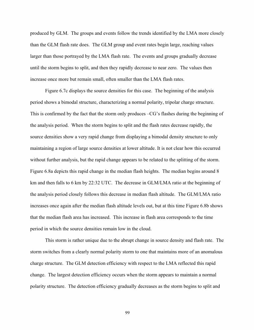
99

produced by GLM. The groups and events follow the trends identified by the LMA more closely

than the GLM flash rate does. The GLM group and event rates begin large, reaching values

larger than those portrayed by the LMA flash rate. The events and groups gradually decrease

until the storm begins to split, and then they rapidly decrease to near zero. The values then

increase once more but remain small, often smaller than the LMA flash rates.

Figure 6.7c displays the source densities for this case. The beginning of the analysis

period shows a bimodal structure, characterizing a normal polarity, tripolar charge structure.

This is confirmed by the fact that the storm only produces –CG’s flashes during the beginning of

the analysis period. When the storm begins to split and the flash rates decrease rapidly, the

source densities show a very rapid change from displaying a bimodal density structure to only

maintaining a region of large source densities at lower altitude. It is not clear how this occurred

without further analysis, but the rapid change appears to be related to the splitting of the storm.

Figure 6.8a depicts this rapid change in the median flash heights. The median begins around 8

km and then falls to 6 km by 22:32 UTC. The decrease in GLM/LMA ratio at the beginning of

the analysis period closely follows this decrease in median flash altitude. The GLM/LMA ratio

increases once again after the median flash altitude levels out, but at this time Figure 6.8b shows

that the median flash area has increased. This increase in flash area corresponds to the time

period in which the source densities remain low in the cloud.

This storm is rather unique due to the abrupt change in source density and flash rate. The

storm switches from a clearly normal polarity storm to one that maintains more of an anomalous

charge structure. The GLM detection efficiency with respect to the LMA reflected this rapid

change. The largest detection efficiency occurs when the storm appears to maintain a normal

polarity structure. The detection efficiency gradually decreases as the storm begins to split and

100

then never regains the same detection efficiency once the storm displays an anomalous structure.

The storm apparently weakens based on a decrease in the reflectivity echo-top heights during the

split (Figure 6.8c). The normal polarity portion of this storm was characterized by flashes

occurring high in the cloud, likely resulting in more photons exiting the top of the cloud as they

have less distance to reach cloud top, leading to the enhanced detection efficiency. As flashes

transition to lower in the cloud, the detection efficiency drops significantly. Towards the end of

the analysis period the detection efficiency increases once again, but this time the flash area has

increased which may have aided in GLM detection of flashes.

6.5 SUMMARY AND CONCLUSIONS

Three preliminary case study analyses were examined for three unique storms observed

during the GLM calibration/validation field campaign mission that took place on 8 May 2017.

This “gold mine” day featured severe, hail producing, storms of both anomalous and normal

polarity charge structure. The Fort Morgan case as well as the beginning periods of the Denver

hail case both displayed normal polarity charge structures. These storms produced the largest

GLM/LMA ratios, that is, the largest GLM flash detection efficiencies. This is likely a result of

flashes occurring at higher altitudes within a cloud. When flashes occur at higher altitudes,

photons emitted by lightning do not have as far of a path to travel before they reach the cloud top

where GLM can detect them. Smaller paths likely lead to less scattering of light, and thus

brighter flashes that are easier for GLM to detect. The Fort Morgan case also showed that

increases in the flash area can lead to enhanced flash detection efficiencies during normal

polarity storms.

The Greeley storm, as well as the end of the Denver hail storm, produced anomalous

charge structures. The Greeley storm was a pure anomalous case, with the majority of the CG

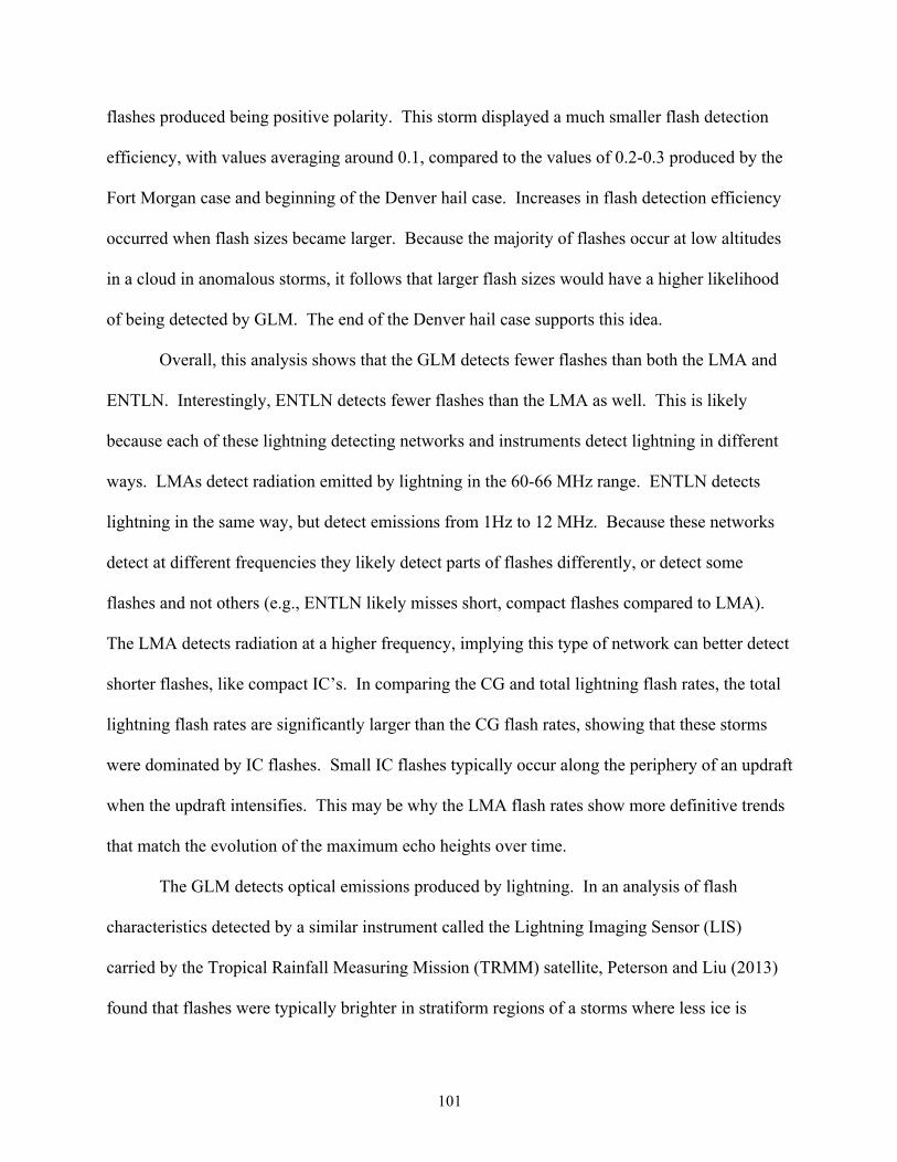
101

flashes produced being positive polarity. This storm displayed a much smaller flash detection

efficiency, with values averaging around 0.1, compared to the values of 0.2-0.3 produced by the

Fort Morgan case and beginning of the Denver hail case. Increases in flash detection efficiency

occurred when flash sizes became larger. Because the majority of flashes occur at low altitudes

in a cloud in anomalous storms, it follows that larger flash sizes would have a higher likelihood

of being detected by GLM. The end of the Denver hail case supports this idea.

Overall, this analysis shows that the GLM detects fewer flashes than both the LMA and

ENTLN. Interestingly, ENTLN detects fewer flashes than the LMA as well. This is likely

because each of these lightning detecting networks and instruments detect lightning in different

ways. LMAs detect radiation emitted by lightning in the 60-66 MHz range. ENTLN detects

lightning in the same way, but detect emissions from 1Hz to 12 MHz. Because these networks

detect at different frequencies they likely detect parts of flashes differently, or detect some

flashes and not others (e.g., ENTLN likely misses short, compact flashes compared to LMA).

The LMA detects radiation at a higher frequency, implying this type of network can better detect

shorter flashes, like compact IC’s. In comparing the CG and total lightning flash rates, the total

lightning flash rates are significantly larger than the CG flash rates, showing that these storms

were dominated by IC flashes. Small IC flashes typically occur along the periphery of an updraft

when the updraft intensifies. This may be why the LMA flash rates show more definitive trends

that match the evolution of the maximum echo heights over time.

The GLM detects optical emissions produced by lightning. In an analysis of flash

characteristics detected by a similar instrument called the Lightning Imaging Sensor (LIS)

carried by the Tropical Rainfall Measuring Mission (TRMM) satellite, Peterson and Liu (2013)

found that flashes were typically brighter in stratiform regions of a storms where less ice is

102

present and flashes are typically larger. They found flashes were typically dimmer in regions

where more ice was present to scatter and attenuate the optical light. The findings of this study

are consistent with the results of Peterson and Lui (2013). GLM seems to detect flashes better

when they occur higher in altitude where they do not need penetrate as much cloud or in

situations where flash sizes are larger.

This preliminary analysis shows that GLM is successfully detecting lightning flashes in

both anomalous and normal polarity storms. Based on this limited sample, the detection

efficiency is rather low for both types of storm, with anomalous polarity storm flashes being the

most difficult for GLM to estimate flash rates within. Further analysis is needed to fully

understand how the dynamics and physical structure of each of these storms relates to the

detection of GLM flashes. By developing a more complete understanding of GLM’s strengths

and weaknesses, the calibration/validation process can be used to improve the GLM instrument

and to prepare forecasters for the new, invaluable data source.

!

!

!!

!

!

!

!

!

!

!

!

!

!

!

!

!

!

!

!

103

!

Figure 6.1 Image and caption taken from Goodman et al. 2013 depicting

how GLM flashes are created from GLM events and groups.

104

Figure 6.2 Visual depiction of the convex hull method for determining the flash area.

Individual dots represents LMA sources. The solid black contour surrounding these dots

represents the convex hull drawn around the flash. The area within this contour is

recorded as the area of the LMA flash. Image taken from Bruning and MacGorman

(2013).

105

Figure 6.3 displays the lightning characteristics of the Fort Morgan normal polarity case. a)

depicts the flash rates produced by the GLM, LMA, and ENTLN in solid contours while the

GLM/LMA ratio is depicted by the dotted line. b) depicts the event rates and group rates

produced by GLM as well as the GLM and LMA flash rates for reference. c) LMA source

densities are binned by 0.5 km intervals and displayed for each radar volume. Warm colors

represent higher source densities. d) NLDN CG flash rates color coded by their polarity.

c)

d)

b)

a)

106

Figure 6.4 displays characteristics of the Fort Morgan normal polarity case. a) displays the

median flash heights determined by the LMA over time b) displays the median flash area

determined by the LMA over time c) displays the maximum reflectivity heights over time of the

35 dBZ contoured storm.

b)

c)

a)

107

Figure 6.5 Same as 6.3 but for the Greeley anomalous polarity case.

a)

b)

c)

d)

108

Figure 6.6 Same as 6.4 but for the Greeley anomalous polarity case.

a)

b)

c)

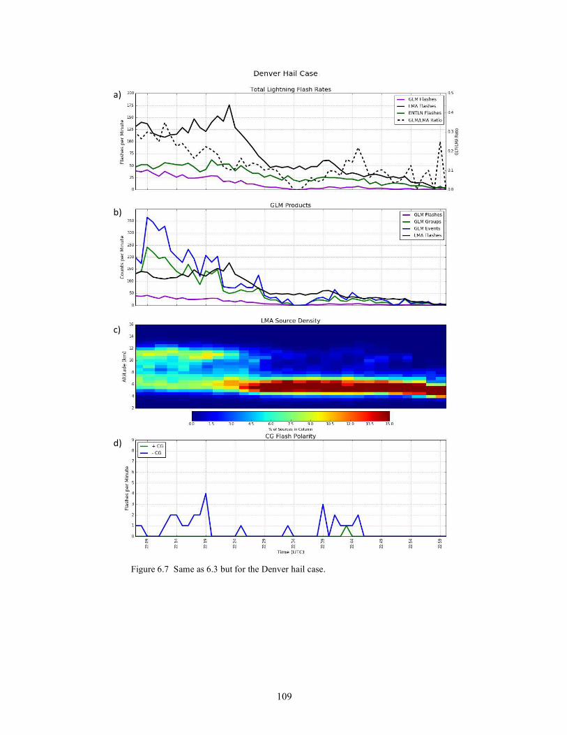
109

Figure 6.7 Same as 6.3 but for the Denver hail case.

a)

b)

c)

d)

110

Figure 6.8 Same as 6.4 but for the Denver hail case.

a)

b)

c)

111

CHAPTER 7: SYNTHESIS

The Geostationary Lightning Mapper (GLM) will provide scientists and forecasters with

continuous access to total lighting data over most of the western hemisphere once GLM becomes

operational. In preparation for the capabilities of GLM, this study related lightning behavior to

the dynamics found within tornadic storms. Lightning flash rates typically increase rapidly, or

“jump”, before severe weather is reported at the surface (Williams et al. 1999; Gatlin and

Goodman 2010; Schultz et al. 2011, 2015, 2017). This is true because total lightning is closely

linked to the updraft characteristics within a storm (Goodman et al. 1988; Dye et al. 1989; Carey

and Rutledge 1994; Williams et al. 1999; Lang and Rutledge 2002; Wiens et al. 2005;

Tessendorf et al. 2007; Deierling et al. 2008; Schultz et al. 2015, 2017).

Multiple studies have found that the total lightning flash rate jumps prior to

tornadogenesis as a result of updraft intensification (Williams et al. 1999; Buechler et al. 2000;

Goodman et al. 2005; Steiger et al. 2005; Steiger et al. 2007; Darden et al. 2010; White et al.

2012; Stano et al. 2014). Updrafts intensify prior to tornadogenesis because an updraft is

necessary to tilt horizontal vorticity found at the surface into the vertical, where it can generate a

mesocyclone (Davies-Jones 1984). A downdraft is then necessary to advect vertical vorticity to

the surface so that a tornado can develop (Markowski 2002; Davies-Jones et al. 2001; Davies-

Jones 2014). Many studies find that total lightning flash rates typically decrease just prior to the

onset of a tornado at the surface, perhaps in relation to this downdraft formation (Williams et al.

1999; Buechler et al. 2000; Steiger et al. 2005, 2007; Darden et al. 2010; White et al. 2012;

Stano et al. 2014). Analysis of four tornadic supercells within this study affirmed these findings.

112

First, two tornadic supercells were analyzed within the domain of the Colorado LMA.

One storm produced an EF3 tornado while the other produced three, short-lived EF0 tornadoes.

Prior to each tornado report, the total lightning flash rates showed a rapid increase associated

with an updraft intensification. Updraft intensifications were inferred to occur when the graupel

volume above freezing level in the storm increased rapidly. Intensifying updrafts lead to more

supercooled liquid water in the mixed phase region, promoting this graupel growth and thus

enhanced flash rates. The presence of KDP and ZDR columns in radar cross sections of these

storms confirmed that the updrafts were lofting oblate, liquid drops above the freezing level to

aid graupel production. LMA source density heights increased in conjunction with increasing

flash rates in two of the four Colorado tornadoes analyzed. These increasing source heights

indicated large scale ascent of the positive charge layer.

After rapidly increasing, the flash rates showed a peak and then decreased prior to the

start of each tornado report. Decreasing graupel volumes occurred in conjunction with

decreasing flash rates, suggesting that graupel fell out of the storm during these time periods.

Increasing rain rates at this time are consistent with a water-laden downdraft. These indications

of downdraft formation were supported by the realization a tornado. Two of the four cases also

exhibited a descent in source density heights, indicating large scale descent of the positive charge

layer as hydrometeors fell through the cloud. This finding is similar to Steiger et al. (2005,

2007) where authors find that flash heights descend during tornado reports.

To determine if the ambient environment affects the relationship between lightning

behavior and storm dynamics, two tornadic supercells were analyzed within range of the North

Alabama LMA. The two Alabama supercells produced smaller flash rates than the Colorado

supercells, but the relationship between lightning behavior and the dynamics that led to

113

tornadogenesis within each storm were similar. Increasing flash rates occurred in conjunction

with intensifying updrafts, while flash rates typically decreased prior to or during tornadogenesis.

One case produced an EF4 tornado that occurred after an increase, peak, and decrease in both the

flash rates and source density heights. The second Alabama case displayed flash rates increasing,

peaking, and decreasing around the time of tornadogenesis, but not necessarily prior to it.

The case study analysis of lightning behavior in four tornadic supercells showed good

agreement with previous literature. The total lightning flash rates revealed information about

what was physically happening in the storm. Increasing flash rates indicated updraft

intensification while decreasing flash rates suggested that a downdraft was forming to help

advect vertical vorticity to the surface. Lightning flash rates were better correlated to storm

dynamics than the source density heights. Though the flash rates differed between the two

environmental regimes, the relationship between the internal dynamics of the storms and their

lightning behavior did not vary. This is a positive result since forecasters want to use GLM to

assist in nowcasting across the entire western hemisphere.

Results from this study and from previous literature indicate that flash rates typically

show an increase, peak, and then decrease prior to tornadogenesis. This trend is not necessarily

related to the formation of a tornado itself; but instead, it is related to the storm dynamics that

allow a supercellular tornado to form. To contrast supercellular tornados and lightning

variability, two landspout tornadoes are analyzed within the domain of the Colorado LMA and

compared to the supercell cases. Landspouts form when vertical vorticity is already present at

the surface. An updraft from a developing storm then stretches the vertical vorticity and pulls it

upward through the atmospheric column, allowing for a landspout to form (Wakimoto and

114

Wilson 1989). Because an updraft is required to maintain a landspout, one would expect flash

rates to continue to increase during landspout formation.

Analysis of the landspout cases revealed that the total lightning flash rates generally

increased during both tornado reports. Increasing graupel and hail volumes, as well as increasing

rain rates occurred in conjunction with the increasing flash rates, indicating that the storms were

in a developmental stage during tornadogenesis. Flash rates peaked and then decreased after the

landspout lifted in both cases. This decrease in flash rate is likely associated with the updraft

weakening, or even the formation of a downdraft (NOTE—in an air mass like storm the

downdraft forms and chokes off the updraft). A weakened updraft is detrimental to a landspout

since the updraft is responsible for pulling vertical vorticity through the atmospheric column.

One case displayed decreasing graupel and hail volumes in conjunction with increasing rain rates

after the landspout lifted. These microphysical characteristics occurred in conjunction with

decreasing flash rates, suggesting that the flash rates were revealing the formation of a downdraft

that led to the termination of the landspout. The source density heights showed no defined

trends in either landspout case.

Results of this study indicate that total lightning flash rates can be used to understand

dynamical and physical processes in a storm. Few regions across the United States have access

to LMA data, so GLM will provide total lightning to many forecasters for the first time. Of

course, GLM must properly detect lighting for the instrument to be truly useful. GLM detects

optical emissions produced by lightning as seen at cloud top. GLM is currently in its

calibration/validation stages and undergoing initial analysis so that problems with the instrument

can be pinpointed and corrected before GLM data becomes operational.

115

Results from limited case study analysis over the Colorado LMA during the GLM

calibration/validation field campaign suggest GLM detection efficiencies of 10-30% when LMA

data is considered “truth”. These values are significantly smaller than the instrument

requirement of 70% detection efficiency. This initial analysis includes three cases studies

characterized by a normal polarity storm, anomalous polarity storm, and a storm that displayed

both normal and anomalous polarity characteristics. The normal polarity cases displayed the

highest detection efficiencies, likely as a result of flashes occurring at higher altitudes compared

to anomalous storms. When flashes occur at higher altitudes, they have less ice to penetrate to

reach the cloud top, reducing the scattering and attenuation of optical light. Results also indicate

the flash size may play a role in detection efficiency, such that larger flashes are more easily

detected by GLM.

One case displayed a purely anomalous charge structure characterized by flashes and

source density heights occurring at low level in the cloud, as well as the smallest detection

efficiency. Radar reflectivity displayed 55 dBZ echo heights reaching 8 km agl for most of the

analysis period. There was no correlation between flash height and detection efficiency, likely as

a result of flash heights occurring low in the cloud, below large values of radar reflectivity.

Perhaps more ice was present between the flashes and cloud top, leading to enhanced attenuation

and scattering of optical emission when compared to the normal polarity cases. This will be a

subject of a future study. The flash area appeared to play the largest role in flash detection

efficiency. The time period in which a separate case displayed anomalous polarity

characteristics also showed smaller detection efficiencies, likely as a result of flashes occurring

at lower altitudes in the cloud once again.

116

While the GLM flash rates showed very small values in comparison to the LMA flash

rates, GLM events and groups that comprise a GLM flash were closer in magnitude to the LMA

flash rates throughout most of the analysis periods. This warrants further investigation of the

clustering algorithm used to assemble GLM groups and events into flashes. The lower detection

efficiencies found in the anomalous polarity cases likely result from large amounts of ice being

present between a flash and cloud top, leading to more attenuation and scattering than would be

found in a normal polarity storm where flashes occur at higher altitudes.

Though GLM is still undergoing various improvements, this preliminary analysis

suggests GLM may under count lightning in anomalous storms if scattering and attenuation of

optical emissions is truly the problem. GLM does not produce the same flash rates as an LMA in

the normal polarity cases analyzed, but it does show similar trends in flash rate indicating that

GLM will likely be useful for understanding storm dynamics in normal polarity storms. It is

important to remember that these conclusions are based on a very small number of case studies

over one region. Continued analysis of anomalous storms and normal polarity storms is needed

to fully understand where GLM performs best and where GLM needs to be improved.

Regardless of the issues presented in this analysis, GLM shows promise in providing forecasters

with a useful tool to monitor storm development and lightning location.

117

REFERENCES

Adlerman, E. J., K. K. Droegemeier, and R. P. Davies-Jones, 1999: A numerical simulation of

cyclic mesocyclogenesis. J. Atmos. Sci., 56, 2045–2069.

American Meteorological Society, cited 2017: "overshooting top". Glossary of Meteorology.

[Available online at http://glossary.ametsoc.org/wiki/Overshooting_top]

American Meteorological Society, cited 2017: "supercell". Glossary of Meteorology. [Available

online at http://glossary.ametsoc.org/wiki/supercell]

Armijo, L., 1969: A Theory for the Determination of Wind and Precipitation Velocities with

Doppler Radars. J. Atmos. Sci., 26, 570–573.

Baker, B., M. B. Baker, E. R. Jayaratne, J. Latham, and C. P. R. Saunders, 1987: The influence

of diffusional growth rates on the charge transfer accompanying rebounding collisions

between ice crystals and soft hail-stones. Q. J. R. Meteorol. Soc., 113, 1193–1215.

Baker, M. B., and J. G. Dash, 1994: Mechanism of charge transfer between colliding ice particles

in thunderstorms. J. Geophys. Res. 94, 8643-8656.

Boccippio, D. J., K. L. Cummins, H. J. Christian, and S. J. Goodman, 2001: Combined satellite-

and surface-based estimation of the intracloud–cloud-to-ground lightning ratio over the

continental United States. Mon. Wea. Rev., 129, 108–122.

Brady, R. H., and E. Szoke, 1989: A case study of nonmesocyclone tornado development in

northeast Colorado: Similarities to waterspout formation. Mon. Wea. Rev., 117, 843-856.

Branick, M. L., and C. A. Doswell, 1992: An observation of the relationship between supercell

structure and lightning ground-strike polarity. Wea. Forecasting,7, 143–149.

Bruning, E. C. and D. R. MacGorman, 2013: Theory and observations of controls on lightning

flash rate spectra. J. Atmos. Sci., 70, 4012–4029.

Brunkow, D., V. N. Bringi, P. C. Kennedy, S. A. Rutledge, V. Chandrasekar, E. A. Mueller, and

R. K. Bowie, 2000: A Description of the CSU–CHILL National Radar Facility. J. Atmos.

Oceanic Technol., 17, 1596–1608.

Buechler, D. E., K. T. Driscoll, S. J. Goodman, and H. J. Christian, 2000: Lightning activity

within a tornadic thunderstorm observed by the Optical Transient Detector (OTD). Geophys.

Res. Lett., 27, 2253–2256.

Carey, L. D., and S. A. Rutledge, 1996: A multiparameter radar case study of the microphysical

and kinematic evolution of a lightning producing storm. Meteor. Atmos. Phys., 59, 33–64.

118

Carey, L. D., and S. A. Rutledge, 1998: Electrical and multiparameter radar observations of a

severe hailstorm. J. Geophys. Res., 103, 13979–14000.

Carey, L. D., W. A. Petersen, and S. A. Rutledge, 2003: Evolution of cloud-to-ground lightning

and storm structure in the Spencer, South Dakota, tornadic supercell of 30 May 1998. Mon.

Wea. Rev., 131, 1811–1831.

Chen, H., V. Chandrasekar, and R. Bechini, 2017: An Improved Dual-Polarization Radar

Rainfall Algorithm (DROPS2.0): Application in NASA IFloodS Field Campaign. J.

Hydrometeor., 18, 917–937.

Cheng, L. and M. English, 1983: A Relationship Between Hailstone Concentration and Size. J.

Atmos. Sci., 40, 204–213.

Crum, T. D. and R. L. Alberty, 1993: The WSR-88D and the WSR-88D Operational Support

Facility. Bull. Amer. Meteor. Soc., 74, 1669–1687.

Cummins, K., M. Murphy, E. Bardo, W. Hiscox, R. Pyle, and A. Pifer, 1998: A combined

TOA/MDF technology upgrade of the U.S. National Lighting Detection Network. Geophys.

Res., 103, 9035–9044.

Cummins, K. and M. Murphy, 2009: An overview of lighting locating systems: History, tech-

niques, and data uses, with an in-depth look at the US NLDN. Electromagnetic

Compatibility, 51, 499–518.

Curran, E. B., R. L. Holle, and R. E. López, 2000: Lightning casualties and damages in the

United States from 1959 to 1994. J. Climate, 13, 3448–3464.

Darden, C. B., D. J. Nadler, B. C. Carcione, R. J. Blakeslee, G. T. Stano, and D. E. Buechler,

2010: Utilizing total lightning information to diagnose convective trends. Bull. Amer.

Meteor. Soc., 91, 167–175.

Dash, J. D., Mason, B. L., Wettlaufer, J.S., 2001. Theory of charge and mass transfer in ice–ice

collisions. J. Geophys. Res. 106, 20395 – 20402.

Davies-Jones, R. P., 1982: A new look at the vorticity equation with application to

tornadogenesis. Proc. 12th Conf. on Severe Local Storms, San Antonio, TX, Amer. Meteor.

Soc., 249–252.

Davies-Jones, R. P., 1984: Streamwise vorticity: The origin of updraft rotation in supercell

storms. J. Atmos. Sci., 41, 2991–3006.

Davies-Jones, R. P., R. J. Trapp, and H. B. Bluestein, 2001: Tornadoes and tornadic

storms. Severe Convective Storms, Meteor. Monogr., No. 50, Amer. Meteor. Soc., 167–222.

119

Davies-Jones, R., 2015: A review of supercell and tornado dynamics. Atmos. Res., 158-159,

274–291.

Deierling, W., and W. A. Petersen, 2008: Total lightning activity as an indicator of updraft

characteristics. J. Geophys. Res., 113, D16210.

Doviak, R. J., V. Bringi, A. Ryzhkov, A. Zahrai, and D. Zrnić, 2000: Considerations for

Polarimetric Upgrades to Operational WSR-88D Radars. J. Atmos. Oceanic

Technol.,17, 257–278.

Dye, J. E., J. J. Jones, W. P. Winn, T. A. Cerni, B. Gardener, D. Lamb, R. L. Pitter, J. Hallet, and

C. P. R. Saunders, 1986: Early electrification and precipitation development in a small,

isolated Montana cumulonimbus. J. Geophys. Res., 91, 1231-1247.

Dye, J. E., W. P. Winn, J. J. Jones, and D. W. Breed, 1989: The electrification of New Mexico

thunderstorms. Part I: The relationship between precipitation development and the onset of

electrification. J. Geophys. Res., 94, 8643-8656.

Fuchs, B. R., and Coauthors, 2015: Environmental controls on storm intensity and charge

structure in multiple regions of the continental United States. J. Geophys. Res.

Atmos., 120, 6575–6596.

Fuchs, B. R., S. A. Rutledge, B. Dolan, L. D. Carey, C. Schultz, 2017: Relationships between

storm charge structure, microphysics and dynamics, submitted to Journal of Geophysical

Research: Atmospheres.

Gatlin, P. N. and S. J. Goodman, 2010: A total lightning trending algorithm to identify severe

thunderstorms. J. Atmos. Ocean Tech., 27, 3–22.

Giangrande, S.E., S. Collis, J. Straka, A. Protat, C. Williams, and S. Krueger, 2013: A Summary

of Convective-Core Vertical Velocity Properties Using ARM UHF Wind Profilers in

Oklahoma. J. Appl. Meteor. Climatol., 52, 2278–2295.

Goodman, S. J., D. E. Buechler, P. D. Wright, and W. D. Rust, 1988: Lightning and precipitation

history of a microburst producing storm. Geophys. Res. Lett.,15, 1185–1188.

Goodman, S. J., and Coauthors, 2005: The North Alabama Lightning Mapping Array: Recent

severe storm observations and future prospects. Atmos. Res., 76, 423–437.

Goodman, S.J., Mach, D., Koshak, W., Blakeslee, R., 2012: GLM lightning cluster-filter

algorithm. Algorithm Theoretical Basis Document, Ver. 3.0 Revised July 30, 2012. NOAA

NESDIS Center for Satellite Applications and Research, Washington, DC (public version

available from the GOES-R Program Office at http://www.goes-

r.gov/products/ATBDs/baseline/ Lightning_v2.0_no_color.pdf, 69 pp.).

120

Goodman S. J., and Coauthors, 2013: The GOES-R Geostationary Lightning Mapper (GLM).

Atmos. Res., 125–126, 34–49.

Helmus, J. J. & Collis, S. M., (2016). The Python ARM Radar Toolkit (Py-ART), a Library for

Working with Weather Radar Data in the Python Programming Language. Journal of Open

Research Software. 4(1), p.e25.

Heymsfield, A. J., and K. M. Miller, 1988: Water vapor and ice mass transported into the anvils

of CCOPE thunderstorms: Comparison with storm influx and rainout. J. Atmos.

Sci., 45, 3501–3514.

Jayaratne, E. R., C. P. R. Saunders, and J. Hallett, 1983: Laboratory studies of the charging of

soft-hail during ice crystal interactions. Quart. J. Roy. Meteor. Soc., 109, 609–630.

Keighton, S. J., H. B. Bluestein, and D. R. MacGorman, 1991: The evolution of a severe

mesoscale convective system: Cloud-to-ground lightning location and storm structure. Mon.

Wea. Rev., 119, 1533–1556.

Klemp, J.B., Rotunno, R., 1983: A study of the tornadic region within a supercell thunderstorm.

J. Atmos. Sci. 40, 359–377.

Knupp, K. R., and Coauthors, 2014: Meteorological overview of the devastating 27 April 2011

tornado outbreak. Bull. Amer. Meteor. Soc., 95, 1041–1062.

Krehbiel, P., R. J. Thomas, W. Rison, T. Hamlin, M. Davis, and J. Harlin, 2000: Lightning

mapping observations in central Oklahoma. Eos, 81 (3), 21–25.

Kumjian, M.R. and A.V. Ryzhkov, 2008: Polarimetric signatures in supercell thunderstorms. J.

Appl. Meteor. Climatol., 47, 1940–1961.

Lang, T. J., and S. A. Rutledge, 2002: Relationships between convective storm kinematics,

precipitation, and lightning. Mon. Wea. Rev., 130, 2492–2506.

Lang, T. J., and Coauthors, 2004: The Severe Thunderstorm Electrification and Precipitation

Study (STEPS). Bull. Amer. Meteor. Soc., 85, 1107–1125.

Lang, T.J. and S.A. Rutledge, 2011: A framework for the statistical analysis of large radar and

lightning datasets: Results from STEPS 2000. Mon. Wea. Rev., 139, 2536–2551.

Lhermitte, R. M., 1968: New developments in Doppler radar methods. Proc. 13th

Radar Meteor.

Conf., Montreal, Amer. Meteor. Soc., 14-17.

Lhermitte, R., and E. Williams,1985: Thunderstorm electrification: A case study. J. Geophys.

Res., 90(D4), 6071–6078

121

Liu, C., and S. Heckman, 2011: The application of total lightning detection and cell tracking for

severe weather prediction. Proc. Fifth Conf. on the Meteorological Applications of Lightning

Data, Seattle, WA, Amer. Meteor. Soc., 8.2.

López, R. E., and J.-P. Aubagnac (1997), The lightning activity of a hailstorm as a function of

changes in its microphysical characteristics inferred from polarimetric radar observations, J.

Geophys. Res., 102(D14), 16799–16813.

MacGorman, D. R., D. W. Burgess, V. Mazur, W. D. Rust, W. L. Taylor, and B. C.

Johnson, 1989: Lightning rates relative to tornadic storm evolution on 22 May 1981. J.

Atmos. Sci., 46, 221–251.

MacGorman, D. R. and K. E. Nielsen, 1991: Cloud-to-ground lightning in a tornadic storm on 8

May 1986. Mon. Wea. Rev., 119, 1557–1574.

Markowski, P.M., 2002. Hook echoes and rear-flank downdrafts: A review. Mon. Weather Rev.

130, 852–876.

Markowski, P. M., and Y. Richardson, 2009: Tornadogenesis: Our current understanding,

forecasting considerations, and questions to guide future research. Atmos. Res., 93, 3–10.

Marshall, T. C., B. Lin, 1992: Electricity in dying thunderstorms. J. Geophys. Res., 97D9, 9913–

9918.

Marshall, T. C., M. Stolzenburg, P. R. Krehbiel, N. R. Lund, and C. R. Maggio, 2009: Electrical

evolution during the decay stage of New Mexico thunderstorms, J. Geophys. Res., 114,

D02209.

Mason, B.L., Dash, J.G., 1999. An experimental study of charge and mass transfer during ice

contact interactions. Proc. 11th Int. Conf. on Atmos. Elec., Huntsville, Alabama, pp. 264–

267.

Mason, B. L., and J. G. Dash, 2000: Charge and mass transfer in ice-ice collisions: Experimental

observations of a mechanism in thunderstorm electrification. J. Geophys. Res., 105, 10,185–

10,192.

McCarthy, J., 1974: Field verification of the relationship between entrainment rate and cumulus

cloud diameter. J. Atmos. Sci., 31, 1028-1039.

Metzger, E. and W.A. Nuss, 2013: The relationship between total cloud lightning behavior and

radar-derived thunderstorm structure. Wea. Forecasting, 28, 237–253.

Mohr, C. G., L. Jay Miller, R. L. Vaughan, and H. W. Frank, 1986: The merger of mesoscale

datasets into a common Cartesian format for efficient and systematic analyses. J. Atmos.

Oceanic Technol., 3, 143–161.

122

Pawar, S. D., and A. K. Kamra, 2007: End-of-storm oscillation in tropical air mass

thunderstorms. J. Geophys. Res., 112, D03204.

Perez, A. H., L. J. Wicker, and R. E. Orville, 1997: Characteristics of cloud-to-ground lightning

associated with violent tornadoes. Wea. Forecasting, 12, 428–437.

Peterson, M., and C. Liu, 2013: Characteristics of lightning flashes with exceptional illuminated

areas, durations, and optical powers and surrounding storm properties in the tropics and inner

subtropics, J. Geophys. Res. Atmos., 118, 11,727–11,740.

Reynolds, S. E., M. Brook, and M. F. Gourley, 1957: Thunderstorm charge separation. J.

Meteor, 14, 426–436.

Rison, W., R. Thomas, P. Krehbiel, T. Hamlin, and J. Harlin, 1999: A GPS-based three-

dimensional lightning mapping system: Initial observations in central New Mexico. Geophys.

Res. Lett., 26, 3573–3576.

Rotunno, R., 1981. On the evolution of thunderstorm rotation. Mon. Weather Rev. 109, 577–

586.

Rotunno, R., and J. B. Klemp, 1985: On the rotation and propagation of simulated supercell

thunderstorms. J. Atmos. Sci., 42, 271-292.

Ryzhkov, A., and D. S. Zrnic, 1998: Discrimination between rain and snow with a polarimetric

radar. J. Appl. Meteor., 37, 1228–1240.

Saunders, C. P. R., W. D. Keith, and R. P. Mitzeva, 1991: The effect of liquid water on

thunderstorm charging. J. Geophys. Res., 96, 11,007– 11,017.

Saunders, C. P. R., and I. M. Brooks, 1992: The effects of high liquid water on thunderstorm

charging. J. Geophys. Res., 97, 14,671–14,676.

Saunders, C. P. R., and S. L. Peck, 1998: Laboratory studies of the influence of the rime

accretion rate on charge transfer during crystal/graupel collisions. J. Geophys. Res., 103,

13,949–13,956.

Schmit, T. J., M. M. Gunshor, W. P. Menzel, J. J. Gurka, J. Li A. S. Bachmeier,

2005: Introducing the next-generation Advanced Baseline Imager on GOES-R. Bull. Amer.

Meteor. Soc., 86, 1079–1096.

Schultz, C. J., W. A. Petersen, and L. D. Carey, 2009: Preliminary development and evaluation

of lightning jump algorithms for the real-time detection of severe weather. J. Appl.

Meteor., 48, 2543–2563.

123

Schultz, C. J., W. A. Petersen, and L. D. Carey, 2011: Lightning and severe weather: A

comparison between total and cloud-to-ground lightning trends. Wea. Forecasting, 26, 744–

755.

Schultz, C. J., L. D. Carey, E. V. Schultz, and R. L. Blakeslee, 2015: Insight into the physical

and dynamical processes that control rapid increases in total flash rate. Wea.

Forecasting, 30, 1591–1621.

Schultz, C. J., L. D. Carey, E. V. Schultz, and R. J. Blakeslee, 2017: Kinematic and

microphysical significance of lightning jumps versus nonjump increases in total flash

rate. Wea. Forecasting, 32, 275–288.

Schumacher, R. S., D. T. Lindsey, A. B. Schumacher, J. Braun, S. D. Miller, and J. L.

Demuth, 2010: Multidisciplinary analysis of an unusual tornado: Meteorology, climatology,

and the communication and interpretation of warnings. Wea. Forecasting, 25, 1412–1429.

Stano, G. T., C. J. Schultz, L. D. Carey, D. R. MacGorman, and K. C. Calhoun, 2014: Total

lightning observations and tools for the 20 May 2013 Moore, Oklahoma, tornadic supercell.

J. Oper. Meteor., 2, 71–88.

Steiger, S. M., R. E. Orville, M. J. Murphy, and N. W. S. Demetriades, 2005: Total lightning and

radar characteristics of supercells: Insights on electrification and severe weather forecasting.

Preprints, Conf. on the Meteorological Application of Lightning Data, San Diego, CA, Amer.

Meteor. Soc., P1.7.

Steiger, S. M., R. E. Orville, and L. D. Carey, 2007: Total lightning signatures of thunderstorm

intensity over north Texas. Part I: Supercells. Mon. Wea. Rev., 135, 3281–3302.

Strader, S. M., and W. Ashley, 2014: Cloud-to-ground lightning signatures of long-lived tornadic

supercells on 27–28 April 2011. Phys. Geogr., 35, 273–296.

Szoke, E. J., M. L. Weisman, J. M. Brown, and T. W. Schlatter, 1984: A subsynoptic analysis of

the Denver tornadoes of 3 June 1981. Mon. Wea. Rev., 112, 790–808.

Takahashi, T., 1978: Riming electrification as a charge generation mechanism in thunderstorms.

J. Atmos. Sci., 35, 1536-1548.

Tessendorf, S. A., K. C. Wiens, and S. A. Rutledge, 2007: Radar and lightning observations of

the 3 June 2000 electrically inverted storm from STEPS. Mon. Wea. Rev., 135, 3665–3681.

Vicente, G., J. C. Davenport, and R. A. Scofield, 2002: The role of orographic and parallax

corrections on real time high resolution satellite rainfall rate distribution. Int. J. Remote

Sens., 23, 221–230.

Wakimoto, R., and J. W. Wilson, 1989: Non-supercell tornadoes. Mon. Wea. Rev., 117, 1113–

1140.

124

Wang, Y. and V. Chandrasekar, 2009: Algorithm for estimation of the specific differential

phase. J. Atmos. Oceanic Technol., 26, 2565–2578.

White, K., B. Carcione, C. J. Schultz, G. T. Stano, and L. D. Carey, 2012: The use of the North

Alabama Lightning Mapping Array in the real-time operational warning environment during

the March 2, 2012, severe weather outbreak in Northern Alabama. Natl. Wea. Assoc.

Newsletter, Oct. 2012, 2–3.

Wiens, K. C., S. A. Rutledge, and S. A. Tessendorf, 2005: The 29 June 2000 supercell observed

during STEPS. Part II: Lightning and charge structure. J. Atmos. Sci., 62, 4151–4177.

Williams, E. R., M. E. Weber, and R. E. Orville, 1989: The relationship between lightning type

and convective state of thunderclouds. J. Geophys. Res., 94, 13,213–13,220.

Williams, E. R., R. Zhang, and D. Boccipio, 1994: Microphysical growth state of ice particles

and large-scale electrical structure of clouds. J. Geophys. Res.,99, 10,787–10,792.

Williams, E. R., and Coauthors, 1999: The behavior of total lightning activity in severe Florida

thunderstorms. Atmos. Res., 51, 245–265.

Williams, E."R., V. Mushtak,D. Rosenfeld, S. Goodman, and D. Boccippio,

2005: Thermodynamic conditions that lead to superlative updrafts and mixed-phase

microphysics, Atmos. Res., 76, 288–306.