


Bahasa
Halaman
Hukum

econstorMake Your Publications Visible.
A Service of
zbwLeibniz-InformationszentrumWirtschaftLeibniz Information Centrefor Economics
Hensvik, Lena; Nordström Skans, Oskar
Working Paper
The skill-specific impact of past and projectedoccupational decline
Working Paper, No. 2019:28
Provided in Cooperation with:IFAU - Institute for Evaluation of Labour Market and Education Policy, Uppsala
Suggested Citation: Hensvik, Lena; Nordström Skans, Oskar (2019) : The skill-specific impact ofpast and projected occupational decline, Working Paper, No. 2019:28, Institute for Evaluation ofLabour Market and Education Policy (IFAU), Uppsala
This Version is available at:http://hdl.handle.net/10419/227848
Standard-Nutzungsbedingungen:
Die Dokumente auf EconStor dürfen zu eigenen wissenschaftlichenZwecken und zum Privatgebrauch gespeichert und kopiert werden.
Sie dürfen die Dokumente nicht für öffentliche oder kommerzielleZwecke vervielfältigen, öffentlich ausstellen, öffentlich zugänglichmachen, vertreiben oder anderweitig nutzen.
Sofern die Verfasser die Dokumente unter Open-Content-Lizenzen(insbesondere CC-Lizenzen) zur Verfügung gestellt haben sollten,gelten abweichend von diesen Nutzungsbedingungen die in der dortgenannten Lizenz gewährten Nutzungsrechte.
Terms of use:
Documents in EconStor may be saved and copied for yourpersonal and scholarly purposes.
You are not to copy documents for public or commercialpurposes, to exhibit the documents publicly, to make thempublicly available on the internet, or to distribute or otherwiseuse the documents in public.
If the documents have been made available under an OpenContent Licence (especially Creative Commons Licences), youmay exercise further usage rights as specified in the indicatedlicence.
www.econstor.eu

INSTITUTE FOR EVALUATION OF LABOUR MARKET AND EDUCATION POLICY
WORKING PAPER 2019:28
The skill-specific impact of past and projected occupational decline
Lena Hensvik Oskar Nordström Skans

The Institute for Evaluation of Labour Market and Education Policy (IFAU) is a research institute under the Swedish Ministry of Employment, situated in Uppsala.
IFAU’s objective is to promote, support and carry out scientific evaluations. The assignment includes: the effects of labour market and educational policies, studies of the functioning of the labour market and the labour market effects of social insurance policies. IFAU shall also disseminate its results so that they become accessible to different interested parties in Sweden and abroad.
Papers published in the Working Paper Series should, according to the IFAU policy, have been discussed at seminars held at IFAU and at least one other academic forum, and have been read by one external and one internal referee. They need not, however, have undergone the standard scrutiny for publication in a scientific journal. The purpose of the Working Paper Series is to provide a factual basis for public policy and the public policy discussion.
More information about IFAU and the institute’s publications can be found on the website www.ifau.se
ISSN 1651-1166

The skill-specifc impact of past and projected
occupational declinea
Lena Hensvikb
Oskar Nordstrom Skansc
Nov 4, 2019
Abstract
Using very detailed register data on cognitive abilities and productive personality traits
for nearly all Swedish males at age 18, we show that employment in the recent past has
shifted towards skill-intensive occupations. Employment growth is monotonically skill bi-
ased in relation to this set of general-purpose transferable skills, despite the well-known
U-shaped (”polarizing”) relationship to occupational wage ranks. The patterns coexist be-
cause growing low-wage occupations tend to employ workers who are comparably skilled
in these dimensions, whereas workers in declining mid-wage occupations instead have less
of these general non-manual skills than suggested by their wages. Employment has pri-
marily increased in occupations where workers have larger-than-average endowments of
verbal and technical abilities and social maturity. Projections of future occupational de-
cline and automation risks are even more skill-biased, but show similar associations to
most of our specifc skill-measures. The most pronounced difference is that occupations
relying on tolerance to stress are projected to decline in the coming decades.
Keywords: Skills, Polarization, Future of Work
JEL classifcations: J21, J31
aWe are very grateful for insightful comments from Adrian Adermon, David Autor, Gerard J. van den Berg, Michael Boehm, Matias Cortes, Peter Fredriksson, Georg Graetz, Magnus Gustavsson, David Margolis, Magne Mogstad and audiences at the University of Bristol, Paris School of Economics, the Stockholm School of Eco-nomics, the OECD ELS seminar, the ULCS Labour Economics Workshop and the Annual UCLS Advisory Board Meeting. The project was funded through Vetenskapsr°adet grant 2018-04581.
bInstitute for evaluation of labor market and education policy (IFAU) and Uppsala Center for Labor Studies (UCLS), e-mail [email protected]
cUppsala University, IFAU, IZA and UCLS, e-mail [email protected].
1

1 Introduction
The labor market impact of current and future technological innovations is a key topic in so-
cial science and in the public debate. Since Autor et al. (2003), much of the research has
analyzed the process through the lens of a task-based framework which emphasizes task- and
occupation-specifc possibilities of automation. A salient pattern documented across countries
and settings is that employment has grown in the highest-paid and the lowest-paid occupations
whereas employment has declined in occupations in the middle of the wage distribution (Autor
et al. (2003), Goos et al. (2009), Acemoglu and Autor (2011), Goos et al. (2014) and Adermon
and Gustavsson (2015)). The fnding of such polarization is important for understanding the
relationship between technical change and wage inequality. The favoured explanation for the
pattern is a sharp decline in the demand for routine-intensive tasks, traditionally performed by
occupations in the middle of the wage distribution (Autor et al. (2003), Goos et al. (2009),
Acemoglu and Autor (2011), Goos et al. (2014), Michaels et al. (2014), Bohm (2015), Cortes
(2016)). In this article, we add to this literature by instead characterizing occupations by the
skill-set of the employees using very detailed Swedish data on pre-market endowments of traits
and abilities. As shown by Fredriksson et al. (2018), the measures capture skills that are val-
ued across the market (i.e. they are general-purpose transferable skills), but they are used with
different intensities in different occupations. The data thus allow us to provide new and di-
rect evidence on the relationship between occupational decline and the overall endowments
of general skills among workers in each occupation. Furthermore, we are able to document
the association between occupational decline and the specifc traits and abilities of workers
within each occupation. As with most of the literature, this analysis focuses on the evolution
in the recent past. But it has been argued that future technological advances will affect a much
broader set of tasks, and hence different types of workers, than changes in the recent past (see
e.g. Mitchell and Brynjolfsson (2017)). To address this issue, we rely on existing projections
about the future occupation-specifc impact of technical change and assess if these projections
suggest that the association between occupational decline and worker skill types is likely to
change in the non-so-distant future.
Our results show that employment growth in the recent past has had a monotonic positive
relationship to occupation-specifc endowments of general skills, despite of the polarizing re-
lationship to occupational wage ranks. The result implies that growing low-wage jobs require
more of these general skills than indicated by their wage ranks, and that declining mid-wage
occupations instead motivated their relatively high wages aspects that do not require any of
the intellectual traits or abilities captured by our data such as, e.g., manual strength, the ability
to cope with hazardous work environments, pure rent-seeking abilities or the ability to per-
form very specifc manual tasks. We further show that occupations which draw on workers
2

with higher-than-average levels of Social Maturity (i.e. extroversion, responsibility and inde-
pendence), Verbal comprehension and Technical abilities have seen particularly strong growth,
whereas occupations where worker skills primarily come in the form of Psychological En-
ergy (i.e. the ability to focus) and problem solving abilities in the form of Inductive reasoning
have declined. The pattern thus varies substantially according to specifc traits and abilities
even within the broader context of cognitive vs. non-cognitive skills, favoring communication-
related components such as verbal comprehension and social maturity over problem-solving
components such as inductive reasoning and the ability to focus. Finally, we repeat the analy-
sis after replacing the actual evolution during the past decades by projected occupational em-
ployment growth from two different sources. We show that the relationship with both wage
ranks (i.e. polarization), overall skill levels (i.e. the monotonic positive association) and skill-
composition are similar to the experiences of the recent past for both of these projections,
despite the fact that the occupations projected to be affected in the future are different from
those affected in the past. This suggests that empirical lessons from the recent past may be
informative about the distributional impact of future technological change. The main differ-
ence to the past is that the projections suggest that the association between overall skill levels
and occupational growth is projected to become even more pronounced and that occupations
projected to shrink rely on workers with relatively high endowments of Emotional Stability
(tolerance to stress) whereas occupations projected to grow instead employ workers endowed
with high levels of Intensity (i.e. activation without external pressure).
The paper is structured as follows: In Section 2 we give a very brief overview of the relevant
literature. Section 3 discusses our data and empirical method. Section 4 presents the main
results. Throughout, we focus on the essentials in the main paper and refer all robustness
checks and extensions to the appendix. Section 5 concludes.
2 Literature
Since Autor et al. (2003) the literature on technical change has to a large extent analyzed the
impact of automation on workers through its impact on the demand for tasks. This approach
replaced the paradigm of Skill Biased Technical Change, see e.g. Card and DiNardo (2002)
for a critical review, which presupposed that technology was factor-augmenting in the sense
that new technology caused a rise in demand for well educated workers, and a decline in the
demand for low educated workers. The task-based approach notes that some tasks are easier
to automate than others suggesting that changes in the demand for labor induced by technolog-
ical advances are best modeled with a production function where output is produced through
performed tasks, some of which can be automated or offshored with the help of technology.
The ensuing empirical literature has taken this idea to the data by exploring information on
3

the task-contents of different occupations and related the employment growth of occupations
to the potential for automation (Autor et al. (2003), Goos et al. (2009), Acemoglu and Autor
(2011), Goos et al. (2014)).1 A salient fnding is that occupations with a large ”routine task”
component have declined due to technological advances. The fact that many of these routine
jobs are found in the middle of the wage distribution implies that the occupational decline has
lead to polarization in terms of employment growth where ”middling” (in the terminology of
Goos et al. (2014)) wage occupations have declined and occupations in the higher and lower
end of the occupational wage spectrum instead have grown. In terms of wage-evolution the im-
pact is somewhat more intricate since displaced workers from middling-wage jobs will provide
additional downward wage pressure on low-wage jobs.
A key insight from the task-based approach is that the link from technical change to worker
skills is mediated by the demand for tasks. But knowing which worker characteristics are
associated with a negative impact of automation is still of key interest, at least from a policy
perspective.2 A noteworthy feature is that much of the literature note that the wage rank can be
considered an all-encompassing measure of skills, and it is thus commonplace to refer to these
patterns as a decline in middle-skilled jobs and a growth of low- and high-skilled jobs (see e.g.
Autor and Dorn (2013) for a discussion). But in order to make progress on the direct impact
on different types of workers it is useful to be more specifc, and in this paper we therefore
differentiate between skill ranks, to be precisely defned below, and wage ranks.
In another set of related studies, with an objective that is less focused on occupational
decline and polarization, researchers have documented the changing market returns to cognitive
vs. non-cognitive skills (Deming (2017), and Edin et al. (2017)) suggesting that the market
returns to specifc skill-types have shifted over time.3
When discussing the future impact of technological change it is clear that different types
of automation may affect different types of workers and thus have different impacts on the
labor market. One way to address this issue is to focus the analysis on particular well-defned
types of innovations. An important example is provided the emerging literature on the impact
of industrial robots pioneered by Graetz and Michaels (2018) and Acemoglu and Restrepo
(2017). The latter analysis uses the task-based approach to tease out the impact of industrial
robots on the overall economy and isolate the channels that determine the overall impact on
employment.4
1Adermon and Gustavsson (2015) provide an analysis on Swedish register data similar to ours. 2See Cortes (2016) for a thorough investigation of the association between occupational decline and worker
demographics. 3Other related studies include Cortes (2016) who discusses the the impact on the demand for skills in the
framework of a general equilibrium model with endogenous sorting of workers into occupations, but do not use direct measures of worker skills in the empirical application. Bohm (2015) estimates task prices under routine-biased technical change and Graetz and Feng (2016) discusses the role of training requirements for polarization.
4Also related is Michaels et al. (2014) who study the interaction between ICT-use and education in a related framework, showing that industries with faster ICT growth have a faster fall in the demand for middle-educated
4

The fact that new innovations, e.g. relying on machine learning algorithms are likely to
affect different segments of the labor markets than past innovations such as industrial robots
makes it diffcult to know, ex ante, to what extent we can extrapolate from recent experiences
when discussing the future impact of automation technologies. Indeed, much of the attention
of policy makers and the general public has been centered around which tasks are most likely
to be automated in the future, and how this will affect different types of workers. As a conse-
quence, public agencies (see e.g. (Nedelkoska and Quintini, 2018)) and groups of researchers
in economics and beyond have spend considerable amounts of effort on trying to project which
types of tasks are most likely to be automated in the near and distant future. Mitchell and Bryn-
jolfsson (2017) provides a recent discussion regarding the factors that determine the automation
potential of different types of tasks. The most well-known examples of occupation-specifc pro-
jections are probably those of the US Bureau of Labor statistics and Frey and Osborne (2017)
which we rely on in this paper.
3 Data and methods
3.1 Outline of the empirical set-up
Our set-up closely follows the conventions in the literature on task-based labor market polar-
ization to facilitate comparisons with earlier studies. We thus rely on occupation-level data for
most of the analysis although we verify that the main patterns also are present at the job-level
as well.
We rank occupations according to mean wages or skills in a start year (2001 in the baseline)
and relate these to the employment growth of the same occupations during a follow-up period
(2001-13 in the baseline). The raw wage data and occupation data (Strukturlonestatistiken) are
drawn from frms’ personnel records using a frm-level sampling frame covering about half of
all employees every year. The baseline time frame is determined by availability of Swedish
data with consistent occupational codes.5 We also add data on routine intensity from Autor and
Dorn (2013) and Goos et al. (2014).
We add information from two additional resources: The frst is data on worker skills from
the Swedish military draft from Fredriksson et al. (2018). Their descriptive data are on the
3-digit occupational level (from 2001) so we use this level of aggregation as our baseline.
Our second additional resource is projections of future ”automation risks” and occupational
employment growth. We draw these from the offcial 10-year projections published by the US
Bureau of Labor Statistics and from the very well-cited study by Frey and Osborne (2017). As
workers. 5Our occupational employment data are downloaded from Statistics Sweden’s web page, see www.scb.se.
5

with the rest of our set-up and data, we take these projections at face value.
3.2 Occupation-specifc skill endowments
We characterize occupation-specifc skill endowments in eight dimensions using data that orig-
inates from the Swedish military service conscription. The data include information on four
cognitive abilities, assessed through written tests, and four non-cognitive productive traits as-
sessed by trained psychologists during an interview, see Mood et al. (2012) for details about
the testing procedure. All of the skills were measured around age 18, i.e. before labor market
entry, for 90 percent of all Swedish males born between 1951 and 1976.6
We will analyse the skills through a joint composite score, and as separate components.
When analysed jointly, the sum of the eight scores provide a broad assessment of each worker’s
set of intellectual, general purpose, transferable skills. Thus, when referring to skill ranks of
occupations, we rank occupations based on the average worker endowments of these general
skills within each occupation, exactly corresponding to the wage ranks used in the polarization
literature. When we analyze the skills separately, we instead rely on the fact that some aspects
of the skill vector are more productive in some jobs than in others.
We use these data as processed by Fredriksson et al. (2018) who used the scores to study
sorting patterns across jobs and occupations. The processed data capture the average skill
endowments in each occupation among workers with at least three years of tenure at the work-
place. This zooms in on workers who have settled in their job, which is a useful indicator for
having the right skill set for the job-specifc tasks, see Fredriksson et al. (2018) for a further
discussion.7 This is potentially important in our context since some transitory workers in low-
wage occupations may be over-skilled labor market entrants (or students) passing through the
occupations, or young workers involved in an, initially quite volatile, search for an appropriate
frst match (see e.g. Jovanovic (1979)). To validate the usefulness of the scores, Fredriksson
et al. (2018) show that i)) all scores are associated with independent wage returns, ii)) that
workers are sorted into jobs where their coworkers have similar types of abilities, and that iii))
workers sort into jobs where the returns to their specifc skills are higher than average.8
We analyse our skill measures after aggregating them to the level of occupations. This
6The tests are graded on a scale from 0 to 40 for some cohorts and from 0 to 25 for others. To achieve comparability across cohorts, we standardize the test scores (mean = 0, standard deviation = 1) within each cohort of draftees.
7Fredriksson et al. (2018) show that experienced workers who enter new jobs or occupations where tenured workers have a similar skill composition as the entrants earn higher wages and stay longer in these jobs. This suggests that tenured workers’ skills refect the skill requirements of these jobs. In contrast, inexperienced hires are more randomly sorted across jobs and therefore separate more often.
8See also Lindqvist and Vestman (2011) for more evidence on the wage and earnings returns to these cognitive-and non-cognitive test scores; H°akanson et al. (2015) for evidence on (changes in) the sorting of workers to frms by cognitive and non-cognitive skills and Edin et al. (2017) for evidence on the changing returns to these cognitive and non-cognitive skills.
6

alleviates potential concerns regarding random measurement errors that arise when analyzing
the data at the individual level (see e.g. the discussion in Edin et al. (2017)).
3.2.1 Cognitive abilities
The data contain four specifc scores measuring cognitive abilities from the written tests. The
scores capture verbal and technical comprehension as well as spatial and inductive abilities.
The verbal and technical comprehension tests are examples of what, e.g., Cattell (1987) refers
to as ”crystallized” intelligence (Ac), while the spatial and inductive tests are examples of
”fuid” intelligence (A f ).9 Crystallized intelligence measures the ability to utilize acquired
knowledge and skills and is thus closely tied to intellectual achievement and therefore also
malleable through policy interventions. Fluid intelligence, on the other hand, captures the
ability to reason and solve logical problems in unfamiliar situations, and should therefore be
independent of accumulated knowledge.10
Below we defne the abilities and list the occupations that are most heavily endowed in each
of these as illustrative examples.11 We frst split all occupations according to the overall skill
rank and extract the most endowed occupation in the low (LTS), mid (MTS) and high (HTS)
overall skill segments respectively:
• Verbal comprehension (Ac). Storage workers (LTS), Librarians (MTS), Medical Doctors
(HTS).
• Technical understanding (Ac). Wood and Paper Processors (LTS), Photographers (MTS),
Architects and Engineers (HTS).
• Spatial ability (A f ). Furniture Carpenters (LTS), Photographers (MTS), University Re-
search/Teaching (HTS).
• Inductive skill (reasoning) (A f ). Storage Workers (LTS), Librarians (MTS) and Medical
Doctors (HTS).
3.2.2 Non-cognitive productive traits
The data contain four specifc scores measuring productive non-cognitive traits assessed by a
trained psychologist. The content of each of these scores are described in great detail in Mood
9The concepts of crystallized and fuid intelligence was originally developed by Cattell (1971). 10Along these lines, Carlsson et al. (2015) study the relationship between schooling and the cognitive test scores
used in this paper. They fnd that that 10 more days of school instruction raises cognitive scores on the crystallized intelligence tests (verbal and technical comprehension) by approximately one percent of a standard deviation, while the fuid intelligence tests are unaffected.
11This description reiterates results from Fredriksson et al. (2018), see their paper for details on actual scores.
7

et al. (2012) and our interpretation and labeling fully rely on their work.12
Below we defne the traits and list the occupations that are most heavily endowed in each
of these in the low (LTS), mid (MTS) and high (HTS) total skill segments as above:13
• Social maturity measures extroversion, responsibility and independence. Restaurant Work-
ers (LTS), Nurses (MTS), Medical Doctors (HTS).
• Emotional Stability measures tolerance to stress. Miners (LTS), Fire Fighters/Security
Guards (MTS), Pilots (HTS).
• Intensity measures activation without external pressure. Miners (LTS), Forestry Workers
(MTS), Police Offcers (HTS).
• Psychological Energy measures perseverance and the ability to focus. Dairy Producers
(LTS), Placement Offcers (MTS) and Medical Doctors (HTS).
3.3 Projections
Our analysis makes use of two sets of projections of the future demand for labor in different
occupations. These are drawn from the US Bureau of Labor Statistics and from Frey and
Osborne (2017). The two projections differ quite substantially in terms of methodology and
aims (see below). For the purpose of this paper, we do not take a stance on which of these
projections are more accurate but instead consider them as interesting objects in their own
right. We choose the two projections based on the the offcial status in the case of BLS and the
massive impact on the public debate in the case of Frey and Osborne (2017).
The US Bureau of Labor Statistics publishes projections of future employment growth by
occupation. These projections are described in detail on the BLS website. The methodology
assesses the future share of each occupation within each industry and then aggregates this up
after assessing the future total labor demand of each industry. It is stated that ”BLS economists
thoroughly review qualitative sources such as scholarly articles, expert interviews, and news
stories, as well as quantitative resources such as historical data and externally produced projec-
tions.” The analysis incorporates ”judgments about new trends that may infuence occupational
demand, such as expanding use of new manufacturing techniques like 3D printing that might
change the productivity of particular manufacturing occupations, or shifts in customer prefer-
ences between different building materials which may affect demand for specifc construction
occupations.” The assessment thus include factors such as expectations of technological inno-
vations, changes in business practices, reorganizations, off-shoring and cross-industry changes
12Nilsson (2017) provides a mapping between these scores and the ”Big Five” personality classifcations, see the Appendix, Table A.1 for details.
13This description reiterates results from Fredriksson et al. (2018), see their paper for details on actual scores.
8

in demand. These assessed trends are then aggregated into an assessment of whether labor
demand will grow or shrink, and if so, by how much. For each occupation that is expected to
change in size, a reason is stated. Examples from the 2016 projections include:
• ”Security guards (All industries): Productivity change - share decreases as improve-
ments in remote sensing and autonomous robots allow security guards to patrol larger
physical areas.”
• ”Chefs and head cooks (Special food services): Demand change - share increases as a
greater emphasis is placed on healthier food in school cafeterias, hospitals, and govern-
ment, requiring more chefs and head cooks to oversee food preparation in these estab-
lishments.”
Edin et al. (2018) use the 1985 version of these projections and verify that they predict
occupation-specifc employment growth in Sweden between 1985 and 2013.14
Our alternative projection is from Frey and Osborne (2017). This paper stresses that the
impact of technological change on the labor market is likely to be different in the future because
developments relying on artifcial intelligence, such as machine learning and mobile robotics,
will enable technology to replace labor across a wide range of non-routine tasks. They go as far
as to argue that recent advances make it ”possible to automate almost any task, provided that
suffcient amounts of data are gathered for pattern recognition”. Instead, only those tasks that
are subject to engineering bottlenecks are insulated against automation. These are tasks defned
by the use of perception and manipulation, creative intelligence, and social intelligence. In the
end, their methodology for defning the automation potential starts from The Occupational
Information Network (O*NET) data on tasks by occupations and then relies on a combination
of subjective assessments by data scientists and a search for “bottleneck-related” task-variables
within O*NET.15
We use the ensuing automation potentials as transformed into the Swedish occupational
classifcation system by Heyman et al. (2016). To achieve comparability to the case of BLS,
we rank the occupations according to their resilience to automation where a high value refers
to a resilient occupation, i.e. an occupation with many bottleneck tasks, whereas low values
instead indicate occupations that are projected to be relatively easy to automate. It can be
noted that (Nedelkoska and Quintini, 2018) show that Sweden and the US have very similar
”automation risks” using a similar strategy as Frey and Osborne (2017) but at a lower level of
aggregation.16
14Despite noise arising from changes in occupational codes, they fnd that a BLS projection index for the US labor market explains 22 percent of the variation in employment growth across these 28 years in Sweden.
15Finger dexterity, Manual dexterity, and Awkward work positions indicate the bottleneck Perception and ma-nipulation. Originality and Fine arts indicate the bottleneck Creative intelligence, Social perceptiveness, Negoti-ation, Persuasion and Caring for Others indicate the bottleneck Social Intelligence.
16The OECD projections are based on the adjusted (relative to Frey and Osborne (2017)) methodology of (Arntz
9

3.4 Data processing
The level of detail is covering 110 occupations characterized by 3-digits according to the
Swedish nomenclature SSYK (closely related to ISCO-88). We exclude military workers. In
addition, we pre-screened the data to check for anomalies and excluded cases where the num-
ber of employees more than doubled between two adjacent years anytime during the 2001-2013
period. This further excludes ”Higher offcials in public services” and ”Manual construction
laborers”.17 These are both tiny occupations and, as we show in the Appendix, including these
does not affect any of our results.
Our baseline strategy is to rely on 3-digit occupations. However, in the Appendix we also
make use of more detailed defnitions of a job by combining occupations and industry groups.
We also include robustness results where we change the time-frame, the functional forms, the
level of aggregation, weighting and so forth. In the interest of presentation, we will, however,
not always refer to the robustness exercises in the running text. When matching the projections
to Swedish nomenclatures, we lose a few additional occupations where the cross-walk was
unsuccessful.
Descriptive statistics are found in Appendix A. These statistics highlight the distinction
between skill-ranks and wage-ranks which we will document more robustly in the empirical
analysis below. While the employment decline has been concentrated to occupations in the
middle of the wage distribution, worker skills do not show a corresponding pattern. Instead,
we fnd clear examples where workers employed in the declining middle-paying occupations
have lower average skills than workers in some of the growing, but low-paying, occupations.
Examples of low-skilled, mid-wage declining occupations are ”Extraction and building trades
workers”, ”Metal, machinery and related trades workers” and ”Offce clerks” Examples of
growing low-paid occupations with higher skills are ”Personal and protective service workers”
and ”Customer service clerks”.
4 Results
4.1 Wage ranks and skill ranks
Most previous studies have found a U-shaped relationship between occupational employment
growth and the initial wage ranks of these occupations. To frst replicate this pattern within
and Gregory, 2016) which provide lower levels of average automation risks than Frey and Osborne (2017). As we show in Appendix D, the arising resilience rank across occupations is, however, very similar across the Frey and Osborne (2017) assessment for the US and the OECD assessment (building on (Arntz and Gregory, 2016)) for Sweden.
17For the former of these, we know that the origin is a restructuring of job titles within the public sector in 2008. For the latter category, we do not have a clear explanation.
10

our data, we rank occupations by their wage in 2001 and relate this rank to their employment
growth in percent between 2001 and 2013. Panel (a) in Figure 1a shows the expected U-shaped
pattern with a decline in the middle-ranked occupations, i.e. polarization. The magnitudes are
very similar to those found in other studies, e.g. Goos et al. (2009) which also included data
for Sweden. This pattern is very robust to alternative treatments of the data as shown by the
various robustness checks supplied in Appendix B.1.
Figure 1b replicates the second well-established empirical regularity; occupations that are
intensive in routine tasks are declining. This relationship is monotonically negative (but of in-
creasing magnitude). Appendix B provide point estimates and further analyses of the interplay
between wage ranks and routine intensity to further confrm that stylized facts arise also within
our data.18
18The routine task index is based on Autor, Levy, and Murnane (2003) and Autor, Katz, and Kearney (2006, 2008) mapped into the European occupational classifcation by Goos et al. (2014). It is constructed from fve original DOT task measures combined to produce three task aggregates: the Manual task measure corresponds to the DOT variable measuring an occupation’s demand for “eye-hand-foot coordination”; the Routine task measure is a simple average of two DOT variables, “set limits, tolerances and standards” measuring an occupation’s demand for routine cognitive tasks, and “fnger dexterity,” measuring an occupation’s use of routine motor tasks; and the Abstract task measure is the average of two DOT variables: “direction control and planning,” measuring managerial and interactive tasks, and “GED Math,” measuring mathematical and formal reasoning requirements. From these three measures the Routine Task Intensity (RTI) index is constructed as the difference between the log of Routine tasks and the sum of the log of Abstract and the log of Manual tasks.
11

0
0 0 0
Oo OJ 0
0
q 0
0
0 0
'-,-----------------~----~
0 0
20
0
40 60 Wage rank in 2001
I o Growth -- Fitted val ues I
80 100
0
0 0 0 0
0 0 0 o 0° .o?;pQ0 6 o~o o
0-~
()o i p ~ 0 ~,--_ 0 • .ir' o o Q Oo Q(5) o q:,Qo o o,oQ o
0, o O ~Qo
0 0
0 0
0 0
'-,-----------------~----~ 20 40 60
Skill rank in 2001
I o Growth -- Fitted values I
80 100
0 0
'-,----------------------~
E8 r i~ C a,
~o
1 .!:o r
20
0
40 60 RTI rank in 2001
I o Growth -- Fitted values I
0 0
0 0
0
80 100
0
o~ L,----------------------~ 20 40 60
Wage rank in 2001 80
-- Skill rank>wage rank o Growth - - - - - Skill rank<wage rank o Growth
100
Figure 1: Employment growth by occupation 2001 to 2013(a) Growth by wage rank (b) Growth by amount of routine tasks
(c) Growth by skill rank (d) Growth by skill-to-wage rank ratio
Note: y-axis displays the percent change in employment between 2001 and 2013 by occupation according to Statistics Sweden’s offcial calculations. Each circle is a 3-digit occupation according to the Swedish Standard of Occupations (SSYK). Circle sizes represent weights, calculated according to employment shares in 2001. Panel (a): x-axis ranks occupations according to mean wages in 2001. Panel (b) x-axis ranks occupations according to routine task intensity from Goos et al. (2014). Panel (c) x-axis ranks occupations according to mean overall skill intensity by tenured employees in 2001 as calculated by Fredriksson et al. (2018). Panel (d): x-axis ranks occupations according to mean wages as in Panel (a) but separates occupations according to whether or not the skill rank (as in panel c) is higher than the wage rank (as in panel a). All lines represent predictions from regression equations on the following form: EmploymentGrowthoccupation = a+ b ∗ Rankoccupation + c ∗ (Rankoccupation)
2, where Rank is defned as the x-axis of the respective panel.
12

Next, we analyse of the relationship between skill ranks and employment growth at the oc-
cupational level. We rank the occupations according to overall skills measured as the sum of
the eight components.19 As a background, it may be useful to know that the skill-wage corre-
lation at the occupational level is 0.72 which implies a strong positive, but non-deterministic,
relationship between the endowments of overall skills and wages.20
Furthermore, within our data, the overall skill requirements of occupations remain very sta-
ble over time. The inter-temporal correlation in occupation-specifc skill endowments between
2001 and 2008, which is the last year for which we have access to the skill data, is 0.96 (see
Appendix fgure B.3 for details).
Figure 1c documents the relationship between overall skill ranks and employment growth.
In clear contrast to Figure 1a, however, we fnd that the relationship between the skill ranks and
employment growth is positive throughout the distribution. The positive slope is statistically
signifcant (see Table B.2 in Apnnedix B), but the quadratic is not.
As with the wage-rank result, this pattern is robust to a number of variations in the model
and the used data (e.g. including outliers, interacting occupations by industry, changing base
years for measuring skills, using broader start and end periods) as shown in Appendix B.2.21
Our results thus imply that the skill-employment association has the opposite sign to the
wage-employment association in the lower part of the wage spectrum. To align the results it is
instructive to split the sample into occupations according to the relative rank, i.e according to
an indicator variable I = Skillrank > Wagerank and show the association between the wage rank
and the employment growth separately for the values of this indicator. As shown in Figure 1d,
employment has grown much more in occupations where Skillrank > Wagerank . This is particu-
larly true in the mid to low part of the wage distribution. For each of these lines, the polarizing
pattern remain, but is much weaker than in the aggregate. The quadratic ft is negative (hence,
declining occupations) for a long range of low skill-to-wage occupations but positive (growing
occupations) in the full range for high skill-to-wage occupations.
This suggest that the declining mid-wage occupations (on average) motivated their higher
wage by factors that are not included in our skill-vector and that the growing low-wage occu-
pations are more intensive in these skills than the wage rank suggests. As an alternative way of
illustrating the same pattern, Table 1 shows that occupations with a higher skill rank than wage
rank had more employment growth in the lower part of the wage distribution.
The analysis discussed above is performed at the occupational level, but the most immediate
consequences of structural change is felt by workers who lose their jobs, regardless of the
19Using weights defned by estimated wage returns for each of the eight components give identical results, see Appendix B.1.
20As shown in Appendix B.1, the association is stronger in the upper part of the wage distribution which is well in line with results on individual data presented in Lindqvist and Vestman (2011).
21The Appendix also discusses the relationships to wage growth known as ”wage polarization” where the results are less clear, both in our setting and the literature in general.
13

impact at the occupational level. Furthermore, we know that workers are systematically sorted
on skills across jobs even within occupations (Fredriksson et al. (2018)). We therefore provide
a complementary analysis at the job level, where we defne a job as a combination of occupation
and establishment. This analysis studies the relationship between initial wage and skill ranks
of each job and the subsequent employment growth within these jobs. This set up thus uses
job-level employment growth, instead of occupation-level employment growth, as the outcome
of interest. The results, shown in Figure 2, suggest that employment growth has a much more
positive relationship to skills than to to wages in the lower part of the distribution also at the
job-level.
Overall, these results thus imply that the declining mid-wage jobs motivated their wages
through other characteristics than those captured by our vector of general-purpose intellectual
skills, whereas the growing low-wage jobs instead seems to employ workers with a dispropor-
tional abundance of such skills. This transformation of labor demand, from (relatively) high
paying jobs with a low need for general intellectual skills to low paying jobs with a high need
for such skills, may be particularly bad news for workers who used to be able to earn relatively
high rents from very specifc manual skills or rent-seeking abilities. A deeper investigation of
the nature of these ”lost” earnings attributes has to be left for future research, but a tentative
discussion is presented in Appendix B.1 which shows that occupations with higher wage ranks
than skill ranks are found in ”high wage frms”, i.e. frms that, in general, pay a higher wage
premium to identical workers.
Table 1: Employment growth and the skills-to-wage relationship
(1) (2) (3) All occupations Low wage High wage
Outcome: Employment growth I[Skillrank > Wagerank] 9.33 18.56** 8.101
(5.902) (8.711) (9.251) R-squared 0.031 0.111 0.017
Note: The dependent variable is the percent change in employment between 2001 and 2013 by occupation ac-cording to Statistics Sweden’s offcial calculations. The independent variable is an indicator taking the value one if Skillrank > Wagerank in 2001. Column 1 shows the association for the full sample. In columns (2) and (3) we divide occupations into low- and high wage occupations defned by the median in the distribution of mean wages among tenured male workers. Robust standard errors are reported in parentheses *** p<0.01, ** p<0.05, * p<0.1.
14

0 .... c <I)
2 o "'"' s et)
Oo ~N
.:. 0,
~~
~ e 0,0
ID > <I) ,o .0 ~ .Q.
" <I)
~~ ~ n_
0 '?
0 20 40 60 80 100 Job wage rank in 1997
0 ....
000 o "' 0 N
.:. 0 ~N
.c ~o e~ Cl
ID > <1)0
]:; .Q. ->O <I)~
o ' i5 <I) ~ o n_"'
0 '?
0 20 40 60 80 100 Job skill rank in 1997
Figure 2: Predicted job-level employment growth by wage and skill ranks (1997-2008)
(a) Job-level growth by wage rank
(b) Job-level growth by skill rank
Note: y-axis displays the predicted percent change in employment between 1997 and 2008 by job defned by the combination of an occupation and an establishment obtained from the following equation: EmploymentGrowth job = a+ b ∗ Rank job + c ∗ (Rank job)
2, where Rank is defned as the x-axis of the respective panel. See Appendix B.1. for details on the data construction.
15
4.2 Specifc skill endowments
Our results presented above rely on an overall measure of skills. But our data allow for an
analysis of the granularity underlying this aggregate score. Which types of skills are more
pronounced among workers in growing vs. shrinking occupations? To analyze this issue, Table
2 shows the relationship between skills and occupational employment growth. We frst show
the coeffcient related to the above discussion on overall skills (column 1), we then redo this
analysis controlling for the wage rank with a quadratic term (column 2), and the association is
only marginally altered.
We then turn to the eight specifc skill measures. The table shows these in the order implied
by the point estimates ranging from the most positive to the most negative estimate. Notably,
the ft of the model is substantially improved when including the specifc skills (adjusted R2
grows from 0.18 to 0.29 and overall R2 from 0.20 to 0.35). As is evident, the associations are
very different for different scores, and these vary also within the groups of cognitive abilities
(indexed by A) and non-cognitive traits (T). The cognitive abilities are separately indicated with
(Ac) for the malleable ”Crystallized” abilities and (A f ) for the less malleable ”Fluid” abilities.
The results show that the “Social maturity” trait as well as the crystallized cognitive abilities
(”Verbal” and ”Technical”) have strong positive associations with employment growth, whereas
the “Psychological energy” trait and the fuid cognitive abilities (primarily “Inductive”) have
negative associations with employment growth conditional on the other skills.
As with the results above, we use the web Appendix (B.2) to show that the associations are
robust to a number of variations in the estimated model.22 The Appendix also shows that verbal
skills are more important as a predictor in high-wage occupations, whereas social maturity and
technical abilities matter more in the low-wage occupations.
22The Appendix also shows the corresponding association between occupational skill measures and routine task content. These results suggest that the same occupational skill endowments associated with occupational growth/decline, are the same endowments associated with lower/higher amount of routine tasks.
16

Table 2: Determinants of employment growth 2001-2013
(1) (2) (3) Overall skills Specifc skills
Panel A: Overall skills: Skill rank 0.263** 0.331**
(0.104) (0.155) Panel B: Specifc skills: Social maturity (T) 1.479*
(0.809) Verbal (Ac) 1.427**
(0.579) Technical (Ac) 1.050**
(0.436) Emotional stability (T) 0.599
(0.718) Intensity (T) 0.035
(0.223) Spatial (A f ) -0.642
(0.532) Psychological energy (T) -1.422*
(0.821) Inductive (A f ) -1.974***
(0.674) Wage rank -1.418*** -1.935***
(0.359) (0.436) Wage rank2 0.013*** 0.016***
(0.004) (0.004) Observations 107 107 107 R-squared 0.068 0.200 0.354 Adjusted R-squared 0.059 0.177 0.287
Note: Dependent variable is percent change in employment between 2001 and 2013 by occupation according to Statistics Sweden’s offcial calculations. Each observation is a 3-digit occupation according to the Swedish Standard of Occupations (SSYK). Regressions are weighted according to employment shares in 2001. Skill rank is a rank of occupations according to mean overall skill intensity by tenured employees in 2001 as calculated by Fredriksson et al. (2018). Wage rank instead ranks occupations according to mean wages in 2001. Specifc skills rank occupations according to skill intensity in each dimension during 2001 as calculated by Fredriksson et al. (2018). The skills are ordered according to estimate size. The different types of skills are highlighted by: T = Non-Cognitive Trait, Ac = Crystallized (malleable) Cognitive Ability and A f = Fluid (less malleable) Cognitive Ability. Interpretation of non-cognitive traits are according to Mood et al. (2012) which provides further details on the tests. Robust standard errors in parentheses *** p<0.01, ** p<0.05, * p<0.1.
17

4.3 Occupational employment projections
Finally, we turn to the projected future. As noted in the introduction, much of the concerns
regarding the labor market impact of future automation rest on the fear that the not-so-distant
future will have an impact on the labor market that is fundamentally different from these ex-
periences. The challenges for doing empirical research on future processes are obvious and
fundamental. To make progress on this front, we rely on the existing projections of future oc-
cupational declines that were described in the data section. We rank the occupations according
to projections to get a comparable metric. Figure 3a plots the association between BLS projec-
tions and wage ranks. It suggests a continued hollowing out of employment in the middle of
the wage distribution. But as we shown for the past above, there is a monotonically positive
relationship between overall skills and future growth (Figure 3b). In Figures 3c and 3d we show
that we get a very similar pattern when we replace the BLS projections with those from Frey
and Osborne (2017). In Panel A of Table 3, we show the regression coeffcients and compare
the results to that of the recent past. As is evident, the skill-bias is projected to increase in
the future. This implies that the occupational decline is projected to continue to favor more
skill-intensive jobs also in the future.
In the foot of Table 3 we show that the predictions are related, but different. The correlation
is 0.46. Furthermore, it is shown that the correlations between each projection and the employ-
ment growth in the recent past is positive (0.22 for Frey and Osborne and 0.34 for BLS), but in
both cases substantially lower than across the two sets of projections.23
Panel B shows the relationship between the projections and the eight sub-components of
our skill-vector. The results, again, show that the two projections produces a very similar pic-
ture despite the large differences in methodology and scope. The results imply that occupations
that (currently) rely on workers with Social Maturity and Verbal comprehension are projected
to continue to grow. Meanwhile, the decline in occupations employing workers with heavy en-
dowments of Inductive reasoning are projected to continue to fall, the results for Psychological
energy are less clear. Thus, in terms of skill-demand, the projections jointly suggest (again, de-
spite their different scopes and methods) that the process of occupational decline will continue
on a similar path as it has in recent decades. The main difference, that arise in both projections,
is a decline in occupations relying on Emotional Stability (i.e. tolerance to stress) and a growth
in occupations relying on Intensity (i.e. activation without pressure). Robustness checks related
to these results are presented in Appendix B.3.
23Examples of occupations that are projected to be exposed to automation in the future, while having proved resilient in the past, include Sales persons, Clerks and Drivers.
18

0 0
0 co
0
"'
0
" 0 N
0 0
0 co
0
" 0 N
Q 0
0 0
0
0 0 (Q) 0
0 .Z§? 0
0 0 0
0 0 0 0 00 0 .°o
0
oo c(jo 0 0
0 8 0
20
0 0
40 60 Wage rank in 2001
0 o 0
80
o Ranked resi lience to automation -- Fitted values
Note: Change is BLS pred ictions for employment growth from 2016 to 2016
0
20
0 0
0
0
0~
0
0
0
0
0
0
0
0 40 60 Wage rank in 2001
0 o.
0
80
o Ranked resi lience to automation -- Fitted values
Note: Resilience ranks based on estimated risks of automation from Frey and Osborne (2013) Conve rted to Swedish nomenclatures by Heyman et al (2016)
0
100
100
0 0
0 co
0
"' 0
" 0 N
0 0
0 co
0
" 0 N
Q O O Q o•o~ cJo 0
0 0 0 0 Ob-1 •
0 0
9 0
Oo 0
0
0
Oo
20
o f() Do .n o" 0 oS, [J
~o O 0
oo
40 60 Skill rank in 2001
0
0
0
80
o Ranked resi lience to automation -- Fitted values
Note: Resilience ranks based on estimated risks of automation from Frey and Osborne (2013) Conve rted to Swedish nomenclatures by Heyman et al 2016)
100
0 0 0
0 0
0 (00 0
0
Q) 0 0 0 0 p
0 000 0
0 0 o0 0 0 o oOO o
0 cP 0
,p 0 0 Q 0 0
0 6)0 0 0 0
20 40 60 80 100 Skill rank in 2001
o Ranked resi lience to automation -- Fitted values
Note: Change is BLS predictions for employment growth from 2016 to 2016
Figure 3: Projected job polarization and skill-bias
(a) Projected polarization (BLS) (b) Projected skill bias (BLS)
(c) Projected polarization (Frey and Osborne) (d) Projected skill bias (Frey and Osborne)
Note: Panels (a) and (b) BLS: y-axis displays the ranked employment change as projected by the US Bureau of Labor statistics transposed into Swedish occupational codes by the authors. Panels (c) and (d) Frey and Osborne: ranked change as projected by Frey and Osborne (2017) transposed into Swedish occupational codes by Heyman et al. (2016). Each circle is a 3-digit occupation according to the Swedish Standard of Occupations (SSYK). Circle sizes represent weights, calculated according to employment shares in 2001. Panels (a) and (c): x-axis ranks occupations according to mean wages in 2001. Panels (b) and (d): x-axis ranks occupations according to mean overall skill intensity by tenured employees in 2001 as calculated by Fredriksson et al. (2018). All lines represent predictions from regression equations on the following form: Pro jectedEmploymentGrowthoccupation = a + b ∗ Rankoccupation + c ∗ (Rankoccupation)
2, where Rank is defned as the x-axis of the respective panel.
19

Table 3: Determinants of past and projected employment growth 2001-2013
(1) (2) (3) Growth: Past Projected: Projected:
BLS Frey & Osborne Panel A: Relationship with overall skills
Skill rank 0.331** 0.647*** 0.788*** (0.155) (0.180) (0.182)
Observations 107 91 103 R-squared 0.200 0.274 0.344
Panel B: Relationship with specifc skills Social maturity (T) 1.479* 2.246** 2.121**
(0.809) (1.030) (0.911) Verbal (A) 1.427** 1.754** 2.125*
(0.579) (0.751) (1.077) Technical (A) 1.050** 0.001 0.674*
(0.436) (0.547) (0.405) Emotional stability (T) 0.599 -1.733** -3.049***
(0.718) (0.777) (0.693) Intensity (T) 0.0348 0.698** 0.966***
(0.223) (0.317) (0.223) Spatial (A) -0.642 0.158 -0.135
(0.532) (0.619) (0.530) Psychological energy (T) -1.422* -0.945 0.176
(0.821) (1.091) (1.005) Inductive (A) -1.974*** -1.723** -2.288*
(0.674) (0.773) (1.307) Observations 107 91 103 R-squared 0.354 0.419 0.557 Correlations: Past growth 1 0.341 0.219 BLS 0.341 1 456 Frey & Osborne 0.219 0.456 1
Robust standard errors in parentheses *** p<0.01, ** p<0.05, * p<0.1
Note: Dependent variables are the change in employment defned as follows: Column (1) The recent past: percent change in actual growth between 2001 and 2013 by occupation according to Statistics Sweden’s offcial calculations. Column (2) Projected BLS: ranked change as projected by the US Bureau of Labor statistics transposed into Swedish occupational codes by the authors. Column (3) Projected Frey and Osborne: ranked change as projected by Frey and Osborne (2017) transposed into Swedish occupational codes by Heyman et al. (2016). Each observation is a 3-digit occupation according to the Swedish Standard of Occupations (SSYK). Regressions are weighted according to employment shares in 2001. Skill rank is a rank of occupations according to mean overall skill intensity by tenured employees in 2001 as calculated by Fredriksson et al. (2018). Model also controls for initial wage rank with squares. Wage rank ranks occupations according to mean wages in 2001. Specifc skills rank occupations according to skill intensity in each dimension during 2001 as calculated by Fredriksson et al. (2018). The skills are ordered according to estimate size in Column (1). The different types of skills are highlighted by: T = Non-Cognitive Trait, Ac = Crystallized (malleable) Cognitive Ability and A f = Fluid (less malleable) Cognitive Ability. Interpretation of non-cognitive traits are according to Mood et al. (2012) which provides further details on the tests. Robust standard errors in parentheses *** p<0.01, ** p<0.05, * p<0.1.
20

5 Conclusions
In this paper, we present a new way of characterizing the skill requirements within occupations
and relate these requirements to occupation-specifc employment trends, in the past and pro-
jected future. Overall, the results provides, what we believe to be, an important addition to the
stock of knowledge regarding the relationship between occupational employment shifts, wage
polarization, and skill demand.
Our results show that occupational employment shifts are skill-biased towards a composite
measure of general-purpose transferable intellectual skills, despite the non-linear relationship
to wages. The reason is that growing low-wage occupations are more intensive in these skills
than their wage ranks suggest and the converse is true for the declining mid-wage occupations.
Focusing on the lower half of the wage distribution, the results thus suggest that labor demand
has moved away from average-paying jobs with a low need for general intellectual skills to-
wards low-paying jobs with a high need for such skills. This process may explain why workers
in declining occupations in the middle of the wage distribution appear to suffer from long-term
adverse employment effects (see e.g. Edin et al. (2018)) as the transition into low-wage jobs
may demand more in terms of general skills than these workers possess, despite of the fact that
their pre-displacement jobs were relatively well paid.
The difference between the skill-rank and wage-rank results arises because our skill mea-
sures are broad in the intellectual dimension but leave out a set of residual unobserved wage-
related attributes such as, e.g., manual strength, the ability to cope with hazardous work envi-
ronments, pure rent-seeking abilities and knowledge that is specifc enough to not be captured
by any of our general skill measures. For natural reasons, we need to leave an exploration of
the relative importance of these unobserved earnings-related factors aside for the purpose of
this article; our results strongly suggest that future research on the granularity of these resid-
ual components and their role in the decline of middling-wage occupations is of frst-order
importance.
Our second key insight is that the underlying patterns are far from uniform across skill
types, even within the broader cognitive vs. non-cognitive aggregates that have been empha-
sized in the related literature on the changing worker-level returns to skills (see Deming, 2017,
and Edin et al 2018). In particular, we note that growing occupations are relatively dense in
Verbal comprehension and Social Maturity (i.e. extroversion), both of which are related to
human communication (and thus perhaps could be labeled ”soft”). Occupations that are dense
in technical abilities have also grown. In contrast, we see and a reduction in employment
within occupations where workers are relatively well-endowed in terms of the ability to fo-
cus (measured as Psychological Energy) and Inductive reasoning, i.e. problem-solving skills.
Notably, and somewhat on the positive side from a policy perspective, both of the cognitive
21

abilities that have seen an increased demand are in the set of (crystallized) abilities that previ-
ous research have identifed as being more malleable since they measure the ability to utilize
acquired knowledge and skills, see e.g. Cattell (1987).
We further show that existing projections, drawn from two very different sources, suggest
that the patterns of the recent past may be reasonably representative of the near future. This
is true even though, as is well known, the same projections suggest that future technology will
affect a very different set of occupations. The relative growth of occupations that (currently)
relies on more skilled workers is projected to continue, perhaps even more distinctly than in
the past. The main consistent projected change is a decline in occupations that employ workers
with higher than average tolerance to stress and a projected growth in jobs that employ workers
with the ability to activate without external pressure. However, since three out of four of the
attributes that defned winners and losers in the recent past will continue to do so in the pro-
jected future, the overall impression is that the same types of workers that gained in the recent
past will be the winners in the near future. On the positive side, this suggest that policy makers
striving to design educational systems to favor the acquisition of skills that are useful at the
future labor market may draw guidance from the evolution in the recent past.
22

References
Acemoglu, D. and Autor, D. (2011), Skills, tasks and technologies: Implications for employ-
ment and earnings, in ‘Handbook of labor economics’, Vol. 4, Elsevier, pp. 1043–1171.
Acemoglu, D. and Restrepo, P. (2017), ‘Robots and jobs: Evidence from us labor markets’.
Adermon, A. and Gustavsson, M. (2015), ‘Job polarization and task-biased technological
change: Evidence from sweden, 1975–2005’, The Scandinavian Journal of Economics
117(3), 878–917.
Arntz, M. and Gregory, T.and Zierahn, U. (2016), ‘The risk of automation for jobs in oecd
countries: A comparative analysis’, OECD Social, Employment, and Migration Working
Papers 189.
Autor, D. H. and Dorn, D. (2013), ‘The growth of low-skill service jobs and the polarization of
the us labor market’, American Economic Review 103(5), 1553–97.
Autor, D. H., Levy, F. and Murnane, R. J. (2003), ‘The skill content of recent technological
change: An empirical exploration’, The Quarterly journal of economics 118(4), 1279–1333.
Bohm, M. (2015), ‘The price of polarization: Estimating task prices under routine-biased tech-
nical change’.
Card, D. and DiNardo, J. E. (2002), ‘Skill-biased technological change and rising wage in-
equality: Some problems and puzzles’, Journal of labor economics 20(4), 733–783.
¨ Carlsson, M., Dahl, G. B., Ockert, B. and Rooth, D.-O. (2015), ‘The effect of schooling on
cognitive skills’, Review of Economics and Statistics 97(3), 533–547.
Cattell, R. B. (1971), ‘Abilities: Their structure, growth, and action’.
Cattell, R. B. (1987), Intelligence: Its structure, growth and action, Vol. 35, Elsevier.
Cortes, G. M. (2016), ‘Where have the middle-wage workers gone? a study of polarization
using panel data’, Journal of Labor Economics 34(1), 63–105.
Deming, D. J. (2017), ‘The growing importance of social skills in the labor market’, The Quar-
terly Journal of Economics 132(4), 1593–1640.
Edin, P.-A., Fredriksson, P., Nybom, M. and Ockert, B. (2017), ‘The rising return to non-
cognitive skill’, IZA, Discussion Paper 10914.
Edin, P.-A., Graetz, G., Hernnas, S. and Michaels, G. (2018), ‘Individual consequences of
occupational decline’, Mimeo, Uppsala University .
23

Fredriksson, P., Hensvik, L. and Nordstrom Skans, O. (2018), ‘Mismatch of talent: Evidence
on match quality, entry wages, and job mobility’, American Economic Review fortcoming.
Frey, C. B. and Osborne, M. A. (2017), ‘The future of employment: how susceptible are jobs
to computerisation?’, Technological Forecasting and Social Change 114, 254–280.
Goos, M., Manning, A. and Salomons, A. (2009), ‘Job polarization in europe’, American eco-
nomic review 99(2), 58–63.
Goos, M., Manning, A. and Salomons, A. (2014), ‘Explaining job polarization: Routine-biased
technological change and offshoring’, American Economic Review 104(8), 2509–26.
Graetz, G. and Feng, A. (2016), ‘Training requirements, automation, and job polarization’,
Economic Journal forthcoming.
Graetz, G. and Michaels, G. (2018), ‘Robots at work’, Review of Economics and Statistics
100(5), 753–768.
H°akanson, C., Lindqvist, E. and Vlachos, J. (2015), Firms and skills: the evolution of worker
sorting, Technical report, Working Paper, IFAU-Institute for Evaluation of Labour Market
and Education Policy.
Heyman, F., Norback, P.-J. and Persson, L. (2016), ‘Digitaliseringens dynamik–en eso-rapport
om strukturomvandlingen i svenskt n¨ or studier i of-aringsliv’, Rapport till Expertgruppen f¨
fentlig ekonomi 4.
Jovanovic, B. (1979), ‘Job matching, and the theory of turnover’, Journal of Political Economy
87, 972–990.
Lindqvist, E. and Vestman, R. (2011), ‘The labor market returns to cognitive and noncogni-
tive ability: Evidence from the swedish enlistment’, American Economic Journal: Applied
Economics 3(1), 101–28.
Michaels, G., Natraj, A. and Van Reenen, J. (2014), ‘Has ict polarized skill demand? evidence
from eleven countries over twenty-fve years’, Review of Economics and Statistics 96(1), 60–
77.
Mitchell, T. and Brynjolfsson, E. (2017), ‘Track how technology is transforming work’, Nature
544(7650), 290–292.
Mood, C., Jonsson, J. O. and Bihagen, E. (2012), Socioeconomic persistence across genera-
tions: The role of cognitive and non-cognitive processes, in J. Ermisch, M. Jantti and T. M.
Smeeding, eds, ‘From Parents to Children: The Intergenerational Transmission of Advan-
tage’, Russell Sage Foundation, chapter 3.
24

Nedelkoska, L. and Quintini, G. (2018), ‘Automation, skills use and training’, OECD Social,
Employment and Migration Working Papers (202).
Nilsson, J. P. (2017), ‘Alcohol availability, prenatal conditions, and long-term economic out-
comes’, Journal of Political Economy 125(4), 1149–1207.
25

Appendix
Abstract
This appendix provides additional information about the data as well as supplementary
analyses and additional results. The appendix is structured in the order of the main paper.
i

Appendix A Supplements to Section on ”Data and methods”
The non-cognitive skill measures capture the workers’ individual traits according to four di-
mensions and in the paper we give a brief description of their interpretation. But to give some
additional favor to their nature it may be useful to highlight how these traits relate to the ”Big
Five” characteristics that are standard measures of personality types used in psychology. Ta-
ble A.1 restates an overview of the relationship from Nilsson (2017) who should be given full
credit for the content. The matrix highlights that ”Social Maturity” mostly captures Extraver-
sion but also some elements of Conscientiousness and Openness/non-conformity. ”Emotional
Stability” is mostly related to Neuroticism. ”Intensity” is a mixture of Conscientiousness and
Openness. Finally, ”Psychological Energy” is most strongly related to Conscientiousness.
Table A.1: Mapping between the cognitive and non-cognitive skills and the ”big fve”
Social maturity Intensity Extraversion (E) The capacity to activate oneself without external pressure (C) Having friends (E) The intensity and frequency of free time activities (O) Taking responsibility (C) Independence (O*) Phsychological energy Emotional stability Perseverance (C) Disposition to anxiety (N) Ability to fulfll plans (C) Ability to control and channel nervousness (-N) To remain focused (C) Tolerance of stress (-N)
Notes: The table shows how the four items that defne the non-cognitive ability test-score from the military enlistment psychologist interview maps into the Big Five traits of Personality inventory. This theory classifes traits into fve broad categories. Openness (O), Conscientiousness (C), Extraversion (E), Agreeableness (A), and Neuroticism (N). The four non-cognitive sub-scales do not match the Big Five traits perfectly. The independence undercategory is interpreted as the alternative interpretation of Openness (O*) which is “non-conformity”. The table (and note) is based on Nilsson (2017).
Table A.2 shows summary statistics for the used sample. While most of our analysis uses
occupational characteristics at the 3-digit level here we list mean employment shares, growth
and skill/wage ranks aggregated to the 2-digit level as in Goos et al. (2014). Following Goos
et al. (2014), we order occupations by their mean wage rank and report the initial employment
share (col 1), and the percentage point change in employment share between 2001-2013 (col 2).
In addition, columns (3) and (4) give the overall skill and wage rank for each occupation group.
It is notable from the table that the highest paying occupations tend to have higher employment
growth, and higher skill levels in the pool of employees. Comparing the skill levels of middle
and low paying occupations this correlation seems less clear and there are several occupations
in the lower part of the wage distribution that have higher skill rank than wage rank. In the
following sections, we will explore in more detail how the skills and wages of occupations
relate to employment growth.
ii
Table A.2: Summary statistics
(1) (2) (3) (4) Occupation ranked by wage Empl. share Empl. Overall skill Wage rank
in 2001 growth rank Highest paying occupations: Legislators and senior offcials 0.03 8.14 89.62 99.06 Corporate managers 3.58 35.07 90.57 96.54 Physical, mathematical and engineering 4.0 23.22 92.45 91.04 science professionals Life science and health professionals 1.97 32.86 88.68 87.11 Other professionals 6.10 19.14 77.36 80.50 General managers 1.80 5.32 66.04 80.19 Physical and engineering science 5.22 6.91 74.15 77.17 associate professionals
Middle paying occupations: Teaching professionals .05 14.18 83.21 62.26 Other associate professionals .09 25.41 69.46 55.07 Other craft and related trades workers .015 39.70 28.30 54.45 Machine operators and assemblers .03 24.88 44.81 51.42 Life science technicians and related .03 7.66 69.10 50.94 associate professionals Subsistence agricultural and fshery workers .05 34.40 25 48.82 Extraction and building trades workers .04 -24.66 33.96 42.92 Metal, machinery and related trades workers .00 -40.76 33.49 37.03 Teaching associate professionals .02 8.46 55.66 36.32 Stationary-plant and related operators .06 -16.72 17.09 36.06 Offce clerks .09 -24.17 44.97 34.12 Sales and services elementary occupations .02 -1.82 6.60 33.49
Low paying occupations: Customer service clerks .02 8.40 52.36 30.19 Personal and protective service workers .16 19.18 45.28 27.74 Models, salespersons and demonstrators .04 38.41 41.51 22.64 Precision, handicraft, printing and .00 -21.62 19.34 19.10 related trades workers Market-oriented skilled agricultural .01 29.12 41.32 16.60 and fshery workers Drivers and mobile-plant operators .04 29.31 3.96 7.55
Note: Statistics are for the used sample but aggregated from the 3-digit to the 2-digit occupational level. Employ-ment growth are for 2001-2013.
iii

Appendix B Supplements to Section on ”Results”
B.1 Supplements to Subsection ”Wage Ranks and Overall Skills”
The frst empirical point made in the paper is that the polarizing relationship between occupa-
tional wage ranks and employment growth is present also in our used data. The second point
is that the relationship to the routine index (RTI) of Autor et al. (2003) is present in the data
as expected. Both of these points are made in Figure 1 in the paper. In Table B.1 we show
the point estimates related to Figure 1a (in column 1) and Figure 1b (in column 2). The table
further shows that the RTI index explains much of the relationship to wage ranks (columns 3
and 4) and, in the fnal column (5), it documents that the relationship between occupational
decline and RTI index also holds within the middle of the wage-rank distribution.
Table B.1: Stylized facts: Job polarization and routine tasks
Dep. var: (1)
Empl. growth (2) RTI
(3) RTI
(4) RTI
(5) RTI
Sample All jobs
All jobs
All jobs
All jobs
Middle wage jobs
Wage rank
Wage rank2
RTI rank
-1.312*** (0.340)
0.014*** (0.003)
0.006 -0.510***
-0.385 (0.415) 0.004
(0.004) -0.461*** -0.902***
RTI rank2 (0.364) -0.005
(0.095) (0.112) (0.204)
Observations 107 (0.004)
94 94 94 30 R-squared 0.162 0.310 0.288 0.295 0.372 Note: The RTI index is only available at the 2-digit level. They are not available for all occupations,
which explains the lower number of observations in columns (2), (3) and (4). *** p<0.01, ** p<0.05, * p<0.1
iv

In Figure B.1, we show that the relationship between employment growth and wage ranks
is robust to a number of different alterations of the used data and the estimated model:
1. In the top left panel (a): We generate more detailed occupational cells by interacting
3-digit occupations and with 10 industry indicators when defning the occupations.
2. In the top right panel (b): We include the two occupations ”Higher offcials in public
services” and ”Manual Construction Laborers” which were excluded in the main analysis
since the data appeared fawed in these occupations due to changes in collection methods
(more than doubled in size across two adjacent years).
3. In the middle left panel (c): We use a smoothed local polynomial instead of the quadratic
functional form employed in the baseline to ensure that the patterns are not forced onto
the data from a too restrictive functional form.
4. In the middle right panel (d): We use wages in offcial statistics to rank the occupations
instead of within-sample wages for tenured males. These data thus do include females
and short tenured males as well. These data also use sample weights that should correct
for under-sampling of small establishments in the micro data. Due to data availability,
we use 2003 as the base year for this analysis.
5. In the lower left panel (e): We vary the start and end point of the analysis. Here we
average over the three frst and the three last years respectively to ensure that the results
are not idiosyncratically related to the specifc years used in the main analysis.
6. In the lower right panel (f): We show the unweighted relationship between the 2001 wage
rank and employment growth. This contrasts to the main analysis which, following the
standards in the literature, are weighted according to the relative sizes of the different
occupations in the start year.
v

a a: Occupation*industry cells
a f ~ ;, -~ .• ·o
"' o,• o• <1)
'• •' 0 Q. • o•. O: . •: • :@O•''t, Sa
r Q 0.
6 0 0 i . ? • 0 . q O Oo ·oOo .. o .. C, q . ?a a. a,. .. 0
~a C <1)
"'o [a • 0 ~
0 0 .; . a·
i b. o oo'? 0, c,o "
Q, 0 . •. 0 o· ·
ci· o(J '. 0 t) • 0 0 • .oo
-~ ~ ·: . i, s 0 (b a 0
6'• · .C?o \o "' <1) a o . °9 :? ~ () a 0-a
20 40 60 80 100 Wage rank in 2001
I 0 Growth --- Fitted values I
a c: Local polynomial
a f ~ "' 0 0 <1) 0 Sa 0 r 00 0 .
0 C 0 <1)
[a 0 0 0 oo i 0 0
00
-~ ~ 0
q 0 <1)
0 :? ~ () a
a
20 40 60 80 100 Wage rank in 2001
I a Growth --- lpoly smooth: Growth I
a e: Changing start and end year for growth
a 0 f ~ "' 0 <1) 0 Sa 0 0 r C <1)
[a 0
i a q -~ ~ 0 a
<1) 0 :? ~ () a
a
20 40 60 80 100 Wage rank in 2001
I 0 Growth --- Fitted values I
a a f ~
"' <1)
Sa
r C <1)
[a 0
i -~ ~ <1)
:? ~ () a
a
a a f ~ 0
"' <1)
Sa
r 0
C <1)
[a 0
i -~ ~ <1)
:? ~ () a
a
a a f ~
"' <1)
Sa
r C <1)
[a 0
i -~ ~ <1)
:? ~ () a
a
20
b: Including all occupations
0
0
0
0
40 60 Wage rank in 2001
0
I o Growth --- Fitted values I
0
80
d: Wage from official statistics (2003 base year)
0
00
0 0
0
20
0
0
00
40 60 Wage rank in 2001
0
0
0
I o Growth --- Fitted values I
0 0
20
0 0
0
f: Unweighted
0 0 0 0
o> o
0 0
0 O
0 0
40 60 Wage rank in 2001
I o Growth --- Fitted values I
0
80
80
100
100
100
Figure B.1: Job polarization: Robustness checks
Note: The Figure shows the relationship between employment growth when we vary the sample and variable defnitions. In (a), we use the combination of 3-digit occupation and broad industry (10 groups) to defne a job; in (b) we include the occupations excluded in our main sample when estimating the quadratic; in (c) we use a local polynomial; in (d), we use wages in offcial statistics instead of within-sample wages for tenured males (due to data availability, we use 2003 as the base year for the analysis). In (e), we use the average of the frst/last three years as the start/end year when calculating employment growth. Finally in (f) we show the unweighted relationship between the 2001 wage rank and employment growth. Each circle is a 3-digit occupation (except in a) according to the Swedish Standard of Occupations (SSYK). Circle sizes represent weights, calculated as employment shares in the start year when applicable.
vi

c Q)
eo Q)O _e,..-~ Cll o
-55 I[)
c Q)
[o 0 c. Eo Q) I[) c , Q)
OlO
~o .c..-(.) '
0 Q
0
0
0 20 40 wagerank
o Managerial work o Technicians and associate professionals o Service and shop sales workers
o Manufacturing Unskilled
0
0
60
0
0
0
0
0
80
Professionals Clerks
100
Forestry and fishing
Machine operators --- Fitted values
A further point of interest is the relationship between occupational decline and different
broad categories of occupations. Figure B.2 therefore illustrates the polarization pattern while
highlighting the different 1-digit occupation groups. As is evident from the fgure, many of
the declining occupations are found in manufacturing jobs and by machine operators. Growing
low-wage jobs are instead drawn from a more mixed set of groups.
Figure B.2: Contribution to polarization by broad occupation groups
Note: y-axis displays the percent change in employment between 2001 and 2013 by occupation according to Statistics Sweden’s offcial calculations. Each circle is a 3-digit occupation according to the Swedish Standard of Occupations (SSYK). Circle sizes represent weights, calculated according to employment shares in 2001. x-axis ranks occupations according to mean wages by tenured employees in 2001. The line represents prediction from the regression equation: EmploymentGrowthoccupation = a+ b∗ Rankoccupation + c∗ (Rankoccupation)
2, where Rank is defned as the x-axis.
After validating the stylized facts the paper goes on to show its main results by focusing
on the relationship between employment growth and occupational skills. The frst main result
is shown in Figure 1c in the main paper and it displays a monotone relationship between oc-
cupational employment growth and occupational skill ranks. The estimates corresponding to
Figure 1c in the main paper are shown in table form in Table B.2. The table also shows that the
square term is insignifcant. Panel B examines whether the results seem sensitive to the way
we measure the overall skill-intensity of an occupation. Instead of using the sum of the eight
talents, we use a weighted sum where the weights correspond to the market wage return of each
skill at age 35, reported in Fredriksson et al. (2018). The estimates look very similar.
Figure B.3 further verifes that the skill-rank of occupation is stable over time. It shows that
there is a strong correlation between occupational skill rank in 2001 and 2008, which is the last
year for which we have access to the skill data. The estimated slope coeffcient is 0.96.
vii

Table B.2: Relationship between skill rank and employment growth
(1) (2) (3) Panel A:Overall skills as sum of talents Skill rank 0.263** 0.331** 0.603
(0.104) (0.155) (0.383) Skill rank2 -0.003
(0.004) Wage rank -1.418*** -1.522***
(0.359) (0.375) Wage rank2 0.013*** 0.015***
(0.004) (0.004) R-squared 0.068 0.200 0.205 Panel B: Overall skills as weighted sum of talents Skill rank 0.258** 0.303* 0.539
(0.105) (0.161) (0.405) Skill rank2 -0.003
(0.004) Wage rank -1.398*** -1.490***
(0.358) (0.375) Wage rank2 0.013*** 0.014***
(0.004) (0.004) R-squared 0.064 0.193 0.197 Observations 107 107 107
Note: The dependent variable is the percent change in employment between 2001 and 2013 by occupation according to Statistics Sweden’s offcial calculations. Each occupation is a 3-digit occupation according to the Swedish Standard of Occupations (SSYK). Column (1) shows the linear relationship between occupational skill rank and employment growth. Column (2) shows the relationship conditional on wagerank and wagerank2. Column (3) shows the quadratic relationship conditional on wagerank and wagerank2. Panel A measures overall skills as the sum of the eight skills. Panel B weights the different skill components by their average wage returns at age 35. The weights are reported in Table 1 in Fredriksson et al. (2018). All regressions are weighted by the occupation employment shares in 2001. Robust standard errors in parentheses *** p<0.01, ** p<0.05, * p<0.1.
viii
.....
0 0
0 co
0 oo N<O C
-'<'. C
~ -0 ~'<t" (I)
0 N
0
0
• • • • •
20
•
•
40 60 Skill rank in 2008
•
80 100
Figure B.3: Stability in occupational skill rank 2001-2008
Note: Each dot represent a 3-digit occupation. Slope coeffcient: 0.9629.
The relationship between wage rank and skill rank
Since this result is very different from the patterns related to the wage ranks, we here let Figure
B.4 show how the wage ranks and skill ranks are associated at the occupational level. As is
evident, there is a strong positive relationship but also with some non-trivial variation around
the prediction line.
Data and functional form
We next show that the relationship between skill ranks and employment growth is robust to
the same variations as we exposed the wage-rank results to in Figure B1 above, i.e. detailed
occupational cells (a), including the two excluded occupations (b) and smoother functional
form (c). The one panel which differs from Figure B1 is the middle right panel (d), where we
show results from using lagged skill endowments (from 1997) instead of using skills from the
same year as the start year of the growth calculation (2001).1 We then proceed as in Figure B1
by showing results varying the start and end point of employment growth (e) and by showing
the unweighted relationship (f).
1This replaces the use of offcial wages in Figure B1 above which has no correspondence for skills.
ix

0 0
0 0
0 0 0 0
0 c5 0
0 (Y So
oO
0 . 00
oc9 <c) 0 0 0
0 0 0
0 0 0 0
Figure B.4: Correlation between 2001 occupational skills and wages.
020
40
60
80
100
Wage r
ank in 2
001
0 20 40 60 80 100Talent rank in 2001
Note: Each dot represent a 3-digit occupation. Circle sizes represent weights, calculated as employment shares in 2001.
x

0 •
0 Qo
0
0, 0
i 0
0
0
a: Occupation*industry cells
· o.,i o • 0
20
20
.o
0
40 60 Ta lent rank in 2001
I o Growth Fitted values I
0
c: Local polynomial
0
0
0
40 60 Talent rank in 2001
0
0
.o
80
80
I o Growth --- lpoly smooth : Growth I
• 0. o •O 9. • •
0 p
100
0
100
e: Changing start and end year for growth 0
0 OQ 0
0 oO • @o O O O ·cw O
0
0 0 ° 0 a ~o O 0
0
20
0
40 60 Talent rank in 2001
0
I o Growth --- Fitted values I
80 100
a a
C: Q)
e Q)
-3ca r C: Q)
EO 1,'
1 -~g
r ug
0 0
o::Joo
20
0
b: Including all occupations
0
40 60 Talent rank in 2001
0
I o Growth Fitted values I
d: 1997 skill levels
0 0
0
Q 0 0
0
0, o crloo oO <c:i
0
0 20
20
0 0
40 60 Talent rank in 2001
I o Growth Fitted values I
f: Unweighted
0 O 0 0
0 0
40 60 Talent rank in 2001
I o Growth Fitted values I
80 100
0 0
0
0
0
80 100
0
0 Oo 0
80 100
Figure B.5: Skill-growth relationship: Robustness checks
Note: The Figure shows the relationship between employment growth and overall skills when we vary the sample and variable defnitions. In (a), we use the combination of 3-digit occupation and broad industry (10 groups) to defne a job; in (b) we include the occupations excluded in our main sample when estimating the quadratic; in (c) we use a local polynomial; in (d), we use a different base year (1997) for calculating the occupational skill-level. In (e), we use the average of the frst/last three years as the start/end year when calculating employment growth. Finally in (f) we show the unweighted relationship between the 2001 wage rank and employment growth. Each circle is a 3-digit occupation (except in a) according to the Swedish Standard of Occupations (SSYK). Circle sizes represent weights, calculated as employment shares in the start year when applicable.
xi

c Q)
~o a,O o....-
~ Cllo -5i LO
c Q)
[o 0 c. E a,O
-~ u;> Q)
g'o coo ..c .,.... o '
0 0 0
0 20 40 talentrank
o Managerial work o Technicians and associate professionals o Service and shop sales workers o Manufacturing
Unskilled
60
0
0
0
0
0
80
Professionals Clerks
100
Forestry and fishing Machine operators Fitted values
As with the wage ranks and fgure Figure B.2 above, it is useful to document the the relation-
ship between skill ranks, occupational decline and different broad categories of occupations.
Figure B.6 therefore illustrate the skill biased patterns while highlighting the different 1-digit
groups. As is evident from the fgure, many of the lowest skilled jobs are in the ”unskilled”
category. This group was much more dispersed in Figure B.2 above.
Figure B.6: Contribution to skill-growth relationship by broad occupation groups
Note: y-axis displays the percent change in employment between 2001 and 2013 by occupation according to Statistics Sweden’s offcial calculations. Each circle is a 3-digit occupation according to the Swedish Standard of Occupations (SSYK). Circle sizes represent weights, calculated according to employment shares in 2001. x-axis ranks occupations according to mean overall skill intensity by tenured employees in 2001 as calculated by Fredriksson et al. (2018). The line represents prediction from the regression equation: EmploymentGrowthoccupation = a+ b ∗ Rankoccupation + c ∗ (Rankoccupation)
2, where Rank is defned as the x-axis.
Grades instead of military skill tests
We further reassess our results using high school school grade point average as our measure of
overall skills. These grades have the advantage of being available for both men and women,
but the disadvantages of mostly capturing cognitive skills (regressing GPA on cognitive and
non-cognitive skills, using individual level data, gives regression coeffcients of 0.66 and 0.22
for cognitive and non-cognitive skills respectively) and having a mechanical relationship to
educational opportunities through admissions system. The main disadvantage is, however, that
GPA does not lend itself to the decomposition that we perform in the rest of the paper. For
the main analysis, it is, however, a reasonable alternative measure. Our analysis of grades in
Figure B.7 has four panels components: First, panel (a), shows that the association between
xii

~
~ ~ ~ ~ 100 Grade rank among males in 2001
Occupationsweightedbytheemploymentshare in2001
O 0 0
z-~
i p
Cl)
E i,O
l CllO
0 """ u
0
~ ~ ~ ~ 100 Grade rank among males in 2001
Occupationsweightedbytheemploymentshare in2001
20 40 60 80 Female grade rank in 2001
0 0 0
0
p
@.o 0
'el
~ ~ ~ ~ Grade rank among women in 2001
Occupationsweightedbytheemploymentshare in2001
100
100
grade ranks and our baseline overall skill rank among males is very strong, second in panel (b)
we show that the association remains potent also if analyzing male conscription tests relative
to female grades within the same occupations. In the lower panels we instead relate the GPA
directly to employment growth, separately for males and females. Both of these associations
are monotonically positive for males (panel c) as well as females (panel d). If anything, the
curvature is the opposite of the polarization (i.e. a more positive slope in the lower part of the
distribution).
Figure B.7: Alternative skill measure: High school grades
(a) Male skill rank- male grade rank (b) Male skill rank- female grade rank
(c) Grade-growth relationship -tenured men
(d) Grade-growth relationship -tenured women
Note: Each circle is a 3-digit occupation according to the Swedish Standard of Occupations (SSYK). Circle sizes represent weights, calculated according to employment shares in 2001. Panel (a) and (b): y-axis ranks occupations according to mean overall skill intensity by tenured male employees in 2001 as calculated by Fredriksson et al. (2018). Panel (a) x-axis ranks occupations according to mean high school grade point average by tenured male employees in 2001. Panel (b): x-axis ranks occupations according to mean high school grade point average by tenured female employees in 2001. Panel (c) and (d): y-axis displays the percent change in employment between 2001 and 2013 by occupation according to Statistics Sweden’s offcial calculations. Panel (c): x-axis displays the grade rank of occupations based on tenured males. Panel (d): x-axis displays the grade rank of occupations based on tenured females.
xiii

Why are the results for skill-ranks different from wage ranks?
As noted in the paper, the difference between the skill-rank and wage-rank results arises be-
cause our skill measures are broad in the intellectual dimension but leave out a set of residual
unobserved wage-related attributes such as, e.g., manual strength, the ability to cope with haz-
ardous work environments, pure rent-seeking abilities and knowledge that is specifc-enough
not be captured by any of our skill measures. A deeper investigation has to be left for future
research, but in order to explore the role for frm-side explanations (i.e. those related to fac-
tors such as hazardous work environments and/or rent-seeking abilities) we have tentatively
explored the relationship between the Skillrank > Wagerank indicator to measures of frm-level
wage premiums. The question we ask is if occupations that are ranked higher in terms of skills
than in terms of wages are more likely to be found in ”high wage frms” defned as frms that,
in general, pay higher wages to identical workers.
To get our measure of frm wage premiums we follow the literature and decompose log
wages into person effects and frm effects (estimated at the establishment level, using the term
”frm effects” for simplicity), according to the AKM-model of (Abowd et al., 1999) :
Yit = θi + ψk(i,t) + Xit β + εit , (B.1)
where Yit is the log wage of worker i in year t, θi is a fxed effect for individual i, ψk(i,t)
is the fxed effect for the employing establishment at year t, Xit β is a set of control variables
(age square and cube and year dummies). We estimate the model on our full micro data set
which covers 1997 to 2009. The estimated frm (ψ) effects are the measures of interest. After
estimating them, we aggregate them to the occupational level using the distribution of occu-
pations across frms during our start year in 2001. Figure B.8 shows the association between
the Skillrank to Wagerank ratio and frm effects across the distribution of frm effects. The clear-
est message that arises from the fgure is that occupations that are associated with low-wage
frms have much higher Skillrank to Wagerank ratio than occupations in in high-wage frms. In
Table B.3, we show the same pattern in a more compact way by instead regressing occupation-
averaged frm-effects on an indicator for Skillrank > Wagerank . The conclusion is very similar.
xiv

0
0 0
0
0 0.
0 0 0 0 0
0 20 60 40 mium in 2001 Firm wage pre
80 100
Figure B.8: Correlation between frm wage premium and the Skillrank to Wagerank ratio
Note: Each circle is a 3-digit occupation according to the Swedish Standard of Occupations (SSYK). Circle sizes represent weights, calculated according to employment shares in 2001. y-axis displays the relationship between the Skillrank and the Wagerank of an occupation. x-axis ranks occupations according to the frm wage premium captured by the estimated frm (ψ) effects from eq. (B.1).
Table B.3: Employment growth and the skills-to-wage relationship
All occupations (1) (2)
Low wage (3)
High wage AKM establishment effect rank -0.011*** -0.010*** -0.008***
(0.002) (0.003) (0.003) R-squared 0.342 0.337 0.268 Observations 107 53 54
Note: The dependent variable is an indicator variable taking the value one if Skillrank > Wagerank and zero oth-erwise, by occupation according to Statistics Sweden’s offcial calculations The independent variable is the frm wage premium captured by the estimated frm (ψ) effects from eq. (B.1). Column 1 shows the association for the full sample of occupations. In columns (2) and (3) we divide occupations into low- and high wage occupations defned by the median in the distribution of mean wages among tenured male workers. Robust standard errors are reported in parentheses *** p<0.01, ** p<0.05, * p<0.1.
xv

Skill ranks, wage ranks and ”Wage Polarization”
The concept of wage polarization refers to the growth of wages at the top and bottom of the
wage rank distribution (see e.g. Acemoglu and Autor (2011)). Here, the results have been less
uniform in the previous literature, which is expected since displaced workers from the middle
of the wage distribution may put additional supply pressure on the low-wage occupations which
may cause these wages to fall even if the demand has a secular increase. In Figure B.9, we show
how wage growth in 2003 (for data availability reasons) to 2013 are related to wage ranks and
skill ranks in 2001. The results show no indications of wage polarization in Sweden during the
period. The patterns for skill ranks are, however, disassociated from wage ranks again since
wage growth appears to have been particularly pronounced in middle skilled occupations.
xvi
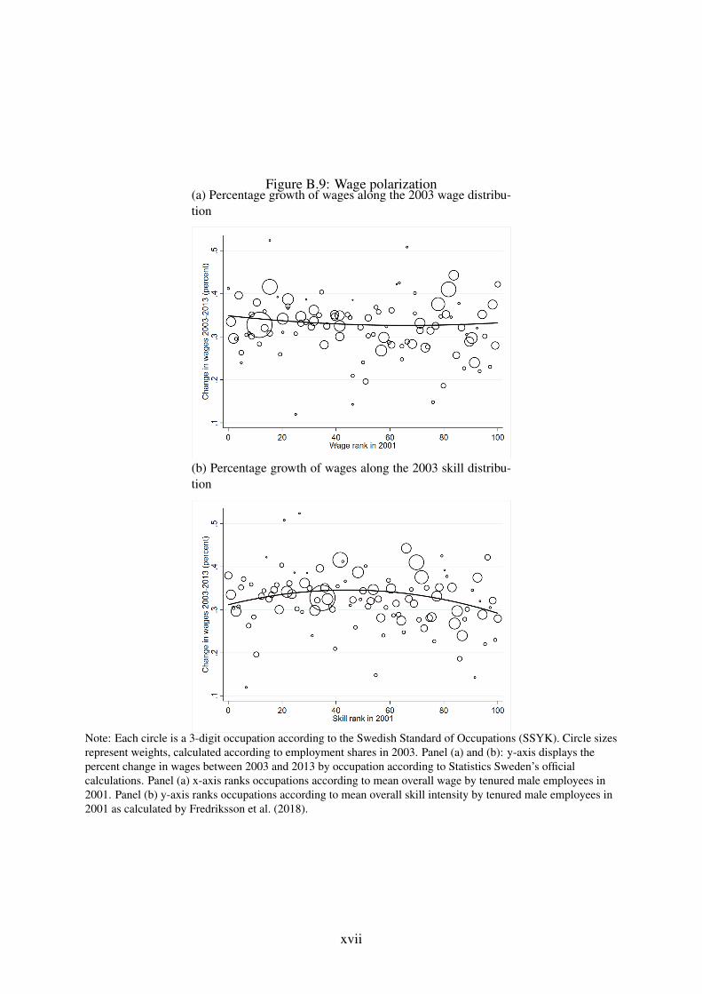
E ~ Q)
s~ ("')
0 N
"' 0 0 NC"'l "' . Q) Ol
~ .!: Q) OlN C .
"' .c u
0 0
0 0 •• 0 0 0 ·9 . . 0 ° 0
cr A O~~ o°oo O u o G (Tu o a o oo n ti& o ~ o
0 O O cJ> o'D (!) 0
0 0 0 0 0 0 0 0
0
0 0 0
0
'"-: l,------,-------,----,-------,-------, 0 20
lO
E Q)
~ Q)
s"": 0 0 ("')
0 N
"' 0 0 NC"'l
"' Q)
Ol 0 "' ;;:
.!: Q) Ol N 0 C
"' .c u
'"-:
0 20
40 60 Wage rank in 2001
G0
o
0
0 0
O°t) 0 (Q) 0 0
0 0
0 0
0
40 60 Skill rank in 2001
80 100
0
0 0
0 0
0
80 100
Figure B.9: Wage polarization(a) Percentage growth of wages along the 2003 wage distribu-tion
(b) Percentage growth of wages along the 2003 skill distribu-tion
Note: Each circle is a 3-digit occupation according to the Swedish Standard of Occupations (SSYK). Circle sizes represent weights, calculated according to employment shares in 2003. Panel (a) and (b): y-axis displays the percent change in wages between 2003 and 2013 by occupation according to Statistics Sweden’s offcial calculations. Panel (a) x-axis ranks occupations according to mean overall wage by tenured male employees in 2001. Panel (b) y-axis ranks occupations according to mean overall skill intensity by tenured male employees in 2001 as calculated by Fredriksson et al. (2018).
xvii

Disappearing jobs
Figure 2 in the paper presents a complementary analysis at the job level where we defne jobs
as occupations within establishments, following Fredriksson et al. (2018). We relate initial
job-level wage and skill ranks to future employment growth within surviving and re-sampled
establishments. We focus on surviving re-sampled establishments to avoid having to make
assumptions about reasons for not being sampled in the outcome year (true exit vs. falling out
of sample frame). We defne our used sample as follows:
• First, we calculate mean wages and skills of male incumbent workers in each job during
our frst year of data (1997). This data include 53,015 distinct jobs.
• Second, we add the total number of paid employees (males and females) to each job.
• Third, we keep establishments that are sampled in 2008 as well. 32,336 distinct jobs
remain.
• Fourth, we add the job-level employment in 2008. If a job observed in 1997 does not
exist within the sampled establishment in 2008, we assume that the job disappeared in
the meantime (i.e. we set N=0 in the fnal year). In total, 6,859 out of our 32,336 jobs
disappeared (21 percent) within our sample of ongoing establishments.
• Fifth, we calculate the employment growth rate from 1997 to 2008 for each of the 32,336
jobs.
• Sixth, we calculate a set of weights according to the initial share of the total employment
within our 32,336 jobs in 1997. This exactly mimics the occupational-level analysis.
The ensuing data gives us growth rates with a mean of 14 percent and a median of -25
percent. The minimum is -100 percent (job exit) and the max is 22,733 percent. As a robustness
check, we have dropped the top one percentile in the growth distribution (new max being 733
percent), which did not change the results in any substantive way. As in the main analysis, we
rank the jobs according to wages and skills and relate second order polynomials of these ranks
to employment growth within these jobs.
xviii

B.2 Supplements to Subsection ”Specifc Skill Endowments”
Table 2 in the paper displays the paper’s second main result. This result shows how the endow-
ments of different types of specifc skills are related to occupational employment growth. There
is substantial heterogeneity between the skill-types within the broader aggregates of cognitive
abilities and non-cognitive traits that have been emphasized in much of the earlier literature.
Figure B.10 shows that the results are robust to a number of variations of the model. To
highlight that the results provide similar rankings, we show the results in panels that display
pairs of the most positive (top) and negative (bottom) associations among the two sets of cogni-
tive abilities and non-cognitive traits respectively. The panels frst show the baseline estimates
of Table 2. In variation (i), we include the two occupations excluded in our main sample; in
(ii), we use the alternative base year (1997) for calculating the occupational skill-level. In (iii),
we use the average of the frst/last three years as the start/end year when calculating employ-
ment growth and in (iv) we show the unweighted relationship between the 2001 wage rank and
employment growth.
We further add two sets of analyses to complete the picture. First, in Table B.4, we show
the associations separately for low-wage occupations and high-wage occupations (splitting by
the median). The results are concurring overall although most of the action for Social Maturity
(positive) and Psychological Energy (negative) arise in the low-wage part whereas the posi-
tive impact of Verbal abilities only is signifcant for high-wage jobs. The negative impact of
Inductive ability arise in both parts of the wage-rank distribution.
Our second additional element relates the skills to the routine index (RTI). Table B.5 repeats
Table 1 of the paper with the RTI as the outcome. The link appears consistent, the routine jobs
that we know are declining more are also employing workers that are less heavily endowed
with skills such as social maturity and technical abilities and have more inductive abilities.
xix

0
"' f§: (/)
'" ] ',---~--~-~--+--~--~-~-~ en -4 -3 -2 -1
'" 1 l,--~--~-~---l-'===~==~~-~-~ en -4 -3 -2 -1
'" 1 L,--~--~-~--'------f----'----~--~-~-~ en -4 -3 -2 -1
:
-4 -3 -2 -1
'" ] ',---~--~-~--+--~--~-~-~ en -4 -3 -2 -1
'" ] l,--~--~-~--'===:t===!:=;::====~ -~-~ en -4 -3 -2 -1
'" ] l,--~--~-'===;:=!:==:J==::'_~--~-~-~ en -4 -3 -2 -1
-5 -4 -3 -2 -1
Figure B.10: Specifc skills-robustness checks(a) Social maturity (b) Verbal skills
(c) Technical skills (d) Emotional stability
(e) Intensity (f) Spatial skills
(g) Phsychological energy (h) Inductive skills
Note: Figures show relationships between employment growth and specifc skills when we vary the sample and variable defnitions. The output come from 5 regressions, one per specifcation. Baseline replicates the estimate from Table 2 in the paper. In (i), we include the two occupations excluded in our main sample when estimating the quadratic; in (ii), we use a different base year (1997) for calculating the occupational skill-level. In (iii), we use the average of the frst/last three years as the start/end year when calculating employment growth and in (iv) we show the unweighted relationship between the 2001 wage rank and employment growth.
xx

Table B.4: Employment growth and specifc skills in low and high wage jobs
Social maturity (T)
Verbal (A)
Technical (A)
Emotional stability (T)
Intensity (T)
Spatial (A)
Psychological energy (T)
Inductive (A)
Observations
(1) All jobs 1.479* (0.809) 1.427** (0.579) 1.050** (0.436) 0.599
(0.718) 0.035
(0.223) -0.642 (0.532) -1.422* (0.821)
-1.974*** (0.674)
107
(2) Low wage 2.842** (1.066) 2.413
(1.584) 1.257*** (0.425) 0.0610 (0.814) 0.172
(0.259) -0.664 (0.537)
-2.065** (0.937) -3.563* (1.823)
53
(3) High wage
0.052 (1.913) 1.902** (0.807) 0.928
(0.987) 0.394
(1.437) 0.0770 (0.497) -0.517 (1.059) -0.289 (1.863) -2.217* (1.225)
54 R-squared Flexible control for wage rank
0.354 Yes
0.435 Yes
0.388 Yes
Note: T = Productive Trait, A = Cognitive Ability. The dependent variable is the percent change in employment between 2001 and 2013 by occupation according to Statistics Sweden’s offcial calculations. Each occupation is a 3-digit occupation according to the Swedish Standard of Occupations (SSYK). Column (1) shows the linear relationship between occupational specifc skill rank and employment growth. In columns (2) and (3) we divide occupations into low- and high-wage occupations defned by the median in the distribution of occupation mean wages. All regressions are weighted by the occupation employment shares in 2001. Robust standard errors in parentheses *** p<0.01, ** p<0.05, * p<0.1.
xxi

Table B.5: Determinants of routine task content
(1) (2) (3) Overall skills Specifc skills
Skill rank -0.010*** -0.003 (0.003) (0.007)
Social maturity (T) -0.089** (0.035)
Verbal (A) -0.031 (0.027)
Technical (A) -0.053** (0.023)
Emotional stability (T) 0.034 (0.024)
Intensity (T) -0.002 (0.010)
Spatial (A) 0.0374 (0.026)
Psychological energy (T) 0.031 (0.031)
Inductive (A) 0.062* (0.035)
Wage rank 0.053*** 0.070*** (0.018) (0.020)
Wage rank2 -0.001*** -0.001*** (0.000) (0.000)
Observations 94 94 94 R-squared 0.075 0.235 0.471
Note: T = Productive Trait, A = Cognitive Ability. The dependent variable is the rank of an occupation according to the routine task intensity (RTI) from Goos et al. (2014). Each occupation is a 3-digit occupation according to the Swedish Standard of Occupations (SSYK). Column (1) shows the linear relationship between occupational specifc skill rank and RTI. Column (2) accounts for the wage rank and column (3) replaces the overall skills with specifc skills (T = Productive Trait, A = Cognitive Ability). All regressions are weighted by the occupation employment shares in 2001. Robust standard errors in parentheses *** p<0.01, ** p<0.05, * p<0.1.
xxii

0 0
Q)
Eo 0 CO .0 (/)
0 ""CJ C tll 0 >,O
~ LL
Q) ()
j~ "iii ~
""CJ Q)
"""o [ijN a::
0
0
0
0
0
0
0
0
0
0
0
0
0
0
0 0
0
0
0
0
0
0
20 40 60 80 Ranked resilience (OECD:s assessment for Sweden)
0
0
0
0
0
100
B.3 Supplements to Subsection ”Occupational Employment Projections”
The fnal set of results in the paper relates the skill measures to projections about future re-
siliance to to automation and general occupational decline. The results are presented in Figure
3 and Table 2 of the paper. In Table B.6, we show the estimated parameters related to polariza-
tion in the past and the projected future corresponding to Figure 3 in the main paper.
In the analysis of the main paper, we rely on projections related to the US that we cross walk
to Sweden. To ensure the validity of these cross-walks, we have also analyzed data from the
OECD where they have redone the Frey and Osborne (2017)-type of resilience calculations for
each country using data from the PIAAC assessments of tasks within each job. These samples
are fairly limited in scope (relative to the data used in this paper) so it is diffcult to use them
at a very detailed occupational level. But, using data at the 2-digit industry level, the ranked
assessments for Sweden appear very well-aligned with the ranked assessments for the US from
Frey and Osborne (2017). The associations are shown in Figure B.11.
Figure B.11: Correlation between US projections and OECD:s Sweden-specifc projection(a) OECD-Frey & Osborne
Note: y-axis ranks occupations according to the projected resilience to automation in Frey and Osborne (2017) for the US. x-axis ranks occupations according to the projected resilience to automation in Nedelkoska and Quintini (2018) for Sweden. The Sweden-specifc projections are calculated using the same task-based approach as in Frey and Osborne (2017), using individual-level survey data (from PIAAC) on the content of tasks in different occupations. The level of observation is the 2-digit industry.
xxiii

—-
Table B.6: Past and projected job polarization
Empl. growth:
Wage rank
Wage rank2
Observations
(1) Past
-1.312*** (0.340)
0.014*** (0.003)
107
(2) Projected:
BLS -1.680** (0.728) 0.016** (0.006)
91
(3) Projected:
Frey & Osborne -0.975 (0.644) 0.012** (0.006)
103 R-squared 0.162 0.156 0.166
Robust standard errors in parentheses *** p<0.01, ** p<0.05, * p<0.1
xxiv
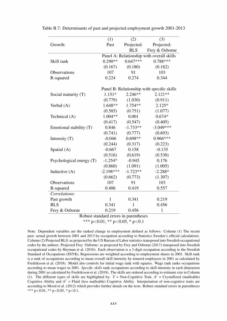
Table B.7: Determinants of past and projected employment growth 2001-2013
(1) (2) (3) Growth: Past Projected: Projected:
BLS Frey & Osborne Panel A: Relationship with overall skills
Skill rank 0.290** 0.647*** 0.788*** (0.167) (0.180) (0.182)
Observations 107 91 103 R-squared 0.224 0.274 0.344
Panel B: Relationship with specifc skills Social maturity (T) 1.151* 2.246** 2.121**
(0.779) (1.030) (0.911) Verbal (A) 1.648** 1.754** 2.125*
(0.585) (0.751) (1.077) Technical (A) 1.004** 0.001 0.674*
(0.417) (0.547) (0.405) Emotional stability (T) 0.846 -1.733** -3.049***
(0.741) (0.777) (0.693) Intensity (T) -0.046 0.698** 0.966***
(0.244) (0.317) (0.223) Spatial (A) -0.667 0.158 -0.135
(0.516) (0.619) (0.530) Psychological energy (T) -1.254* -0.945 0.176
(0.860) (1.091) (1.005) Inductive (A) -2.198*** -1.723** -2.288*
(0.662) (0.773) (1.307) Observations 107 91 103 R-squared 0.406 0.419 0.557 Correlations: Past growth 1 0.341 0.219 BLS 0.341 1 0.456 Frey & Osborne 0.219 0.456 1
Robust standard errors in parentheses *** p<0.01, ** p<0.05, * p<0.1
Note: Dependent variables are the ranked change in employment defned as follows: Column (1) The recent past: actual growth between 2001 and 2013 by occupation according to Statistics Sweden’s offcial calculations. Column (2) Projected BLS: as projected by the US Bureau of Labor statistics transposed into Swedish occupational codes by the authors. Projected Frey Osborne: as projected by Frey and Osborne (2017) transposed into Swedish occupational codes by Heyman et al. (2016). Each observation is a 3-digit occupation according to the Swedish Standard of Occupations (SSYK). Regressions are weighted according to employment shares in 2001. Skill rank is a rank of occupations according to mean overall skill intensity by tenured employees in 2001 as calculated by Fredriksson et al. (2018). Model also controls for initial wage rank with squares. Wage rank ranks occupations according to mean wages in 2001. Specifc skills rank occupations according to skill intensity in each dimension during 2001 as calculated by Fredriksson et al. (2018). The skills are ordered according to estimate size in Column (1). The different types of skills are highlighted by: T = Non-Cognitive Trait, Ac = Crystallized (malleable) Cognitive Ability and A f = Fluid (less malleable) Cognitive Ability. Interpretation of non-cognitive traits are according to Mood et al. (2012) which provides further details on the tests. Robust standard errors in parentheses *** p<0.01, ** p<0.05, * p<0.1.
xxv

References
Abowd, J. M., Kramarz, F. and Margolis, D. N. (1999), ‘High wage workers and high wage
frms’, Econometrica 67(2), 251–333.
Acemoglu, D. and Autor, D. (2011), Skills, tasks and technologies: Implications for employ-
ment and earnings, in ‘Handbook of labor economics’, Vol. 4, Elsevier, pp. 1043–1171.
Autor, D. H., Levy, F. and Murnane, R. J. (2003), ‘The skill content of recent technological
change: An empirical exploration’, The Quarterly journal of economics 118(4), 1279–1333.
Fredriksson, P., Hensvik, L. and Nordstrom Skans, O. (2018), ‘Mismatch of talent: Evidence
on match quality, entry wages, and job mobility’, American Economic Review fortcoming.
Frey, C. B. and Osborne, M. A. (2017), ‘The future of employment: how susceptible are jobs
to computerisation?’, Technological Forecasting and Social Change 114, 254–280.
Goos, M., Manning, A. and Salomons, A. (2014), ‘Explaining job polarization: Routine-biased
technological change and offshoring’, American Economic Review 104(8), 2509–26.
Heyman, F., Norback, P.-J. and Persson, L. (2016), ‘Digitaliseringens dynamik–en eso-rapport
om strukturomvandlingen i svenskt n¨ or studier i of-aringsliv’, Rapport till Expertgruppen f¨
fentlig ekonomi 4.
Mood, C., Jonsson, J. O. and Bihagen, E. (2012), Socioeconomic persistence across genera-
tions: The role of cognitive and non-cognitive processes, in J. Ermisch, M. Jantti and T. M.
Smeeding, eds, ‘From Parents to Children: The Intergenerational Transmission of Advan-
tage’, Russell Sage Foundation, chapter 3.
Nedelkoska, L. and Quintini, G. (2018), ‘Automation, skills use and training’, OECD Social,
Employment and Migration Working Papers (202).
Nilsson, J. P. (2017), ‘Alcohol availability, prenatal conditions, and long-term economic out-
comes’, Journal of Political Economy 125(4), 1149–1207.
xxvi
Top Related
Copyright © 2022 FDOKUMEN

