THE LIQUIDITY EFFECT IN ALGERIA AND MOROCCO: A MULTIVARIATE THRESHOLD

AUTOREGRESSIVE INVESTIGATION 1

Mohamed Benbouziane, Abdelhak Benamar, and Mustapha Djennas

Working Paper 525

June 2010

Send correspondence to: Mohamed Benbouziane Faculty of economics and management, Tlemcen University B.P. 226, Tlemcen, 13000, Algeria. Tel/Fax: 00 213 43 21 21 66 Email: mbenbouziane@yahoo.fr

1 This paper was presented at the Economic Research Forum 16th Annual Conference (Equity and Economic Development 07 - 09 November 2009, Cairo, Egypt) and benefited from financial support from ERF.

First published in 2010 by The Economic Research Forum (ERF) 7 Boulos Hanna Street Dokki, Cairo Egypt www.erf.org.eg Copyright © The Economic Research Forum, 2010 All rights reserved. No part of this publication may be reproduced in any form or by any electronic or mechanical means, including information storage and retrieval systems, without permission in writing from the publisher. The findings, interpretations and conclusions expressed in this publication are entirely those of the author(s) and should not be attributed to the Economic Research Forum, members of its Board of Trustees, or its donors.

1

Abstract:

The objective of this paper is to test for the liquidity effect in Algeria and Morocco using multivariate threshold autoregressive model (MVTAR) as proposed by Tsay (1998). Our empirical results have several important implications. First, results do not support threshold behavior in the case of Algeria. Moreover, when using M1 as a proxy of monetary policy, the liquidity effect hypothesis is rejected in this country. When using bank deposit assets (BDA), results show that there is a negative relationship between monetary shocks and interest rate, and accordingly accepting the liquidity effect. Secondly, in the case of Morocco, however, results show an asymmetric response of interest rate to positive and negative shocks of monetary policy. Moreover, these results strongly support a threshold behavior when BDA is employed, while weakly supporting the same behavior using M1. Furthermore, and using the proxy of bank deposit assets, the liquidity effect are accepted in the low inflation regime, whereas it is rejected in the high inflation regime. Hence, the threshold behavior offers an interesting alternative for explaining the relationship between interest rates and monetary policy shocks. The results presented herein may give more insights on the transmission mechanism of monetary policy in different inflationary environments. Accordingly, a good inflation targeting policy would yield better results in this context. Indeed, the liquidity effect breaks down for the high inflation regime, as inflationary expectations are immediately responsive to money growth. In a low-inflation regime, however, money is not considered to be neutral, as it could affect output through the liquidity effect.

ملخص

ي د التراجع وذج الح ن خالل استخدام نم ر م ي المغرب و الجزائ ي دولت الھدف من ھذا البحث ھو اختبار تأثیر السیولة ف

: أوال. لنتائجنا التجریبیة عدة تضمینات مھمة.1998التلقائي متعدد المتغیرات علي النحو الذي اقترحھ العالم تساي في عام

ة M1 انھ عند استخدام , أضف إلي ذلك. بالنسبة للجزائر ال تدعم النتائج سلوك الحد ة النقدی یًال للسیاس ة , وك ترفض نظری

ین ال . تأثیر السیولة في تلك الدولة لبیة ب ة س ي وجود عالق دمات وعند استخدام أصول الودائع المصرفیة تدل النتائج عل ص

ة المغرب : ثانیا .ومن ثم قبول تأثیر السیولة, النقدیة ومعدل الفائدة ائج بالنسبة لدول ي وجود استجابة , تدل النت ك عل مع ذل

أن ھذه النتائج تدعم مسلك الحد , أضف لذلك. معدل الفائدة للصدمة االیجابیة والسلبیة بصورة غیر متناسقة للسیاسة النقدیة

ع المصرفیة بصورة قویة عندما تستخ د استخدام , دم أصول الودائ لوك عن نفس الس ائج ل م ھذه النت ا یضعف دع .M1 بینم

نخفض , وعالوة علي ذلك خم الم ام ذي التض ي النظ فمع استخدام تفویض أصول الودائع المصرفیة یحظي تأثیر السیولة ف

لوك . بینما یبوء بالرفض في النظام ذي التضخم المرتفع, بالقبول ان س ین ومن ثم ف ة ب ائقًا لتفسیر العالق دیًال ش دم ب الحد یق

وقد تعطي النتائج التي ُقدمت في ھذا البحث مزیدًا من اإلیضاحات .أسعار الفائدة وبین الصدمات الخاصة بالسیاسة النقدیة

جاد معوالت مناسبة فان السیاسة التي تستھدف إی, ووفقا لذلك. بشان آلیة النقل للسیاسة النقدیة في البیئات التضخمیة المختلفة

فان تأثیر السیولة یخفق في حالة النظام ذي التضخم المرتفع , وفي الحقیقة .للتضخم قد تؤدي إلي نتائج أفضل في ھذا السیاق

دي ار . حیث تتسم التوقعات التضخمیة بسرعة االستجابة بطریقة مباشرة للنمو النق ن اعتب ال یمك ك، ف ن ذل رغم م ي ال وعل

.حیث یمكن للنقود أن تؤثر علي الناتج من خالل تأثیر السیولة, نظام منخفض التضخمالنقود محایدًا في

2

1. Introduction

Although the question of how, and to what extent, monetary policy can affect the economy is very controversial, monetary economists and policy makers accept the proposition that, in the short run, changes in the money supply can induce changes in short-term nominal interest rates of the opposite sign. This is called the liquidity effect (LE). Indeed, traditional economic theories hold that expansionary monetary policy can generate a transitory decline in nominal interest rates. A key element in the transmission from money supply to interest rates is the short-run stickiness of prices in the labor and goods market. Therefore, the increase in money supply leads to an increase in real money balances and an excess supply. As the real money supply increases, economic agents become more liquid and adjust their portfolios by buying more bonds. This bids up real bond prices and generates a liquidity effect by decreasing the nominal interest rate, Guirguis (1999). A negative short-run response of interest rates to an exogenous increase in money supply (the liquidity effect proposition) is important in the literature for several reasons. First, conventional wisdom about the transmission mechanism of monetary policy tells us that an increase in money supply has a powerful direct influence on expenditure if it lowers interest rates. Therefore, the effectiveness of monetary policies requires the existence of the liquidity effect. The liquidity effect is secondly also a structural element in monetarist models. In the conventional analysis of the monetarist models of Friedman (1968) and Cagan (1972) both domestic and market labor supplies do not change significantly between the two dates which points out that an increase in money supply depresses the nominal interest rate in the short run, but the expected inflation effect caused by the increase in money supply will dominate the liquidity effect in the long run. Finally, the liquidity effect has important implications for the construction of quantitative macroeconomic models with money. In early monetary real business cycle models, a surprise monetary expansion raises nominal interest rates since interest rate money dynamics are dominated by strong anticipated inflation effects. Christiano (1992) argues that the liquidity effect is an important characteristic that any good model should have.

In spite of the importance of the liquidity effect in theoretical models and policy concerns, its empirical support has yielded mixed results in the literature.

In general, papers based on single equation methods fail to detect a liquidity effect (Mishkin, 1982; Reichenstein, 1987; Thornton, 2001).

Moreover, the majority of empirical studies are based almost entirely on linear vector autoregression (VAR) models. Standard linear time series analysis fails to detect the role of nonlinear variables that could be regarded as propagator of shocks as envisioned in much of the recent theoretical literature on monetary policy.

Accordingly, the objective of this paper is to test for the liquidity effect in the Maghreb Countries (Algeria, Morocco and Tunisia) using a nonlinear framework based on a multivariate threshold autoregressive model (MVTAR) as proposed by Tsay (1998).

Our empirical results have several important implications. First, results do not support threshold behavior in the case of Algeria. Moreover, when using M1 as a proxy of monetary policy, the liquidity effect hypothesis is rejected in this country. When using bank deposit assets (BDA), results show that there is a negative relationship between monetary shocks and interest rate, and accordingly accepting the liquidity effect.

Secondly, in the case of Morocco, however, results show an asymmetric response of interest rate to positive and negative shocks of monetary policy. Moreover, these results strongly

3

support a threshold behavior when BDA is employed, while weakly supporting the same behavior using M1. Furthermore, using the proxy of bank deposit assets, the liquidity effect is accepted in the low inflation regime, whereas it is rejected in the high inflation regime.

Hence, the threshold behavior offers an interesting alternative for explaining the relationship between interest rates and monetary policy shocks.

The results presented herein may give more insights on the transmission mechanism of monetary policy in different inflationary environments. Accordingly, a good inflation targeting policy would yield better results in this context. Indeed, the liquidity effect breaks down for the high inflation regime, as inflationary expectations are immediately responsive to money growth. In a low-inflation regime, however, money is not considered to be neutral, as it could affect output through the liquidity effect.

The remainder of the paper is structured as follows. Section 2 describes some previous empirical studies. We use a nonlinear framework based on a multivariate threshold autoregressive model (MVTAR) as proposed by Tsay (1998) in Section 3 as well as the description of data. Test results are given in Section 4. Finally, concluding remarks are provided in the last section.

2. Some Previous Empirical Studies Although the relationship between money and the interest rate is straightforward in theory, empirical evidence of a liquidity effect has been puzzling. Historically, the theoretical explanation of the liquidity effect was considered plausible and researchers focused on estimating the strength and persistence of the interest rate decline in response to growth of the money stock.

Cagan and Gandolfi (1969), using monthly data in the US from 1910 to 1965, find that a 1% increase in the growth rate of M2 leads to a maximum decline in the commercial paper rate of 2.6%. Melvin (1983), however, undermines the reliance on a simple theoretical relationship by discussing the vanishing liquidity effect and shows that the liquidity effect disappears within a month after the increase in money growth rate in the 1970s due to a dominant anticipated inflation effect.

Using an efficient markets approach, Mishkin (1982) finds that interest rate innovations derived from the term structure are positively related to unanticipated money growth. Grier (1986) demonstrates that Mishkin's results are robust to sample and specification changes. More recent empirical studies have been unable to find evidence of a systematic negative relationship between monetary innovations and interest rates. For instance, and using VAR methods, Sims (1992), finds a positive relationship between money and short-term interest rates. Reichenstein (1987) finds similar results obtained from estimating an equation where a distributed lag of money growth is regressed upon interest rate changes. Thornton, (2001) based on single equation methods fails to detect a liquidity effect.

Cochrane (1989) uses a spectral band pass filter technique to reestablish the liquidity effect from 1979 to 1982.

To investigate for the influence of other variables on the relationship between money and the interest rate, Leeper and Gordon (1992) estimate a four-variable VAR model (money growth rates, interest rates, the consumer price index (CPI) and industrial production). They find no liquidity effect since the relation between the monetary base and the federal funds rate is never negative.

4

Using simple cross-correlation analysis between the federal funds rate and different monetary aggregates, Christiano and Eichenbaum (1992) show that broad monetary aggregates used in the previous studies are inappropriate for identifying the existence of the liquidity effect due to their large endogenous component because changes in broad aggregates reflect both demand and supply shocks creating the money endogeneity problem.

Christiano and Eichenbaum (1992) also argue that the quantity of non-borrowed reserves (NBR) is the best indicator for the policy stance. With NBR included in a VAR model instead of broad money supply, the fed funds rate exhibit a sharp, persistent decline. Thus, using another proxy for monetary policy rather than the monetary base (M1) would be a better indicator.

Bernanke and Blinder (1992) suggest that the Fed watches the fed funds rate closely and conclude that changes in this rate could be used as measure of policy shock. Strongin (1995) proposes using the proportion of NBR growth that is orthogonal to total reserve growth as a policy measure. This author shows that including this measure in a VAR model estimated on sub-samples similar to those used by Leeper and Gordon (1992) yields a highly significant and persistent liquidity effect.

3. Research Methodology The majority of previous studies have used VAR models. Beaudry and Koop (1993), Potter (1995), and Pesaran and Potter (1996), however, have shown that linear models are too restrictive. The authors argue that linear models have a symmetry property which implies that shocks occurring in a recession are just as persistent as shocks occurring in an expansion. Thus, linear models cannot adequately capture asymmetries that may exist in different macroeconomic models. In this section we present the MVTAR model that we will be using in our empirical work. Appropriate hypotheses and test structures are discussed. 3.1. The MVTAR Model MVTAR models are models that could take different regimes. Each regime can be represented by a VAR model. However, the switching of the regime is governed by a switching variable so that any crossing above or below the threshold will trigger the regime to change. These models are presented by Tsay (1998) as follows:

푌 = 푓 (푌 ,푌 , … ; 휀 |휃 ) 푖푓 푧 ≤ 푟푓 (푌 ,푌 , … ; 휀 |휃 ) 푖푓 푧 > 푟 (1)

where Y = (M1 (ou BDA), interest rate, consumer price index, industrial production)′, f (. ) is a function defined as f (. ) ≠ f (. ) if i ≠ j, θ are parameters with finite dimensions, is a positive integer representing the delay of the switching variable z that should be stationary (Hansen, 1996) (In our case, this variable is the rate of inflation (CPI)). In his work, Tsay (1998) uses a linear model that depends on a vector of endogenous variables Y , and a V- dimension vector of exogenous variables X = (X , … , X )′, with r ∈ Γ = r, r , is an interval (usually balanced) of the possible threshold values. In these conditions, Tsay (1998) notes that Y i follows an MVTAR model with a switching variable lagged d period, if it satisfies the following form:

푌 = 푐 + ∑ ∅( )푌 + ∑ 훽( )푋 + 휀( ) 푖푓 푟 ≤ 푧 ≤ 푟 (2)

with j = 1, … , s, c vectors of constants, and are numbers of non-negative integers. The satisfied innovations ε( ) = ∑ a/ , and ∑ / symmetrical positive matrixes and defines, {a } as a sequence of random vectors that are not auto-correlated with a 0 mean and a covariance

5

matrix covariance I (the identical matrix). The switching variable is stationary with a continuous distribution. This model with s regimes is considered linear in the threshold space z , but non linear in time where s > 1.

For the estimation of model (2), Tsay (1998) adopts a generalization of the results of Chan (1993) and Hansen (1996) of the univariate case. To simplify, the model is written in:

푌 =푋 Φ + ∑ 푎/ if 푧 ≤ 푟푋 Φ + ∑ 푎/ if 푧 > 푟

(3)

Where 푎 = (푎 , … ,푎 )′, 푧 is stationary and continuous with a density function 푓(푟) on a defined subset function of the real line 푅 ⊂ 푅, 푑 ∈ {1, … , 푑 }. 푑 is a fixed positive integer. In order to estimate the parameters of model (3) (Φ ,Φ ,∑ ,∑ , 푟 , 푑), Tsay (1998) uses two stage conditional least squares. First, and taking into account the values of 푑 and 푟, model (3) is divided into two multivariate linear regressions with the least squares estimators of Φ et ∑ (with 푖 = 1,2) :

Φ (푟 ,푑) = 푋 푋( )

푋 푌( )

And

∑ (푟 ,푑) = ∑ ∗ ( ∗)( )

(4)

With ∑( ) the sum of all the observations in the regime 푖, Φ∗ = Φ (푟 , 푑), 푛 the number of observations in the regime 푖, and 푘 is the dimension of 푋 (푘 < 푛 푓표푟 푖 = 1,2). The sum of the squared errors is:

푆(푟 ,푑) = 푆 (푟 ,푑) + 푆 (푟 ,푑)

With 푆 (푟 , 푑) the trace of (푛 − 푘)∑ (푟 ,푑). Secondly, the estimators of the conditional least squares of 푟 and 푑 are obtained by:

푟̂ ,푑 = argmin 푆(푟 , 푑)

With 1 ≤ 푑 ≤ 푑 and 푟 ∈ 푅 . The results of the estimators of the least squares of (4) are: Φ = Φ 푟̂ , 푑

And ∑ = ∑ 푟̂ , 푑

To establish the asymptotic properties of these estimators, Tsay (1998) adopts the same approach of Chan (1993) and Hansen (1996). To test for the non linearity of the model (i.e. test for the significance of the MVTAR model against the VAR model), Hansen (1996) proposes the Wald test. In this test, the null hypothesis is: Φ = Φ , which means that the coefficients are equal for the two regimes (the alternative hypothesis for the non linearity is Φ ≠ Φ ). However, the difficulty of this test resides in the existence of the nuisances parameters2. Indeed, the threshold 푟 is not defined under the null hypothesis. In these conditions, when the errors are iid, the most powerful statistic test is the F statistic which is as follows:

퐹 = sup ∈ 퐹(푟 ) 2 The problem of the nuisance parameters non-identified under the null hypothesis is well explained in Ploberger (1994), Hansen (1996), and Stinchcombe and White (1998).

6

Due to the fact that 푟 is not identified, this statistic does not follow a chi-square distribution. To overcome this problem, Hansen (1996) proposes an approximation with the bootstrap procedure. 3.2 The Generalized Response Functions In this paper, we use an MVTAR model to analyze the impact of monetary policy shocks on the interest rate in the Maghreb countries. We are exploring the impact of the variables change of the monetary policy on the interest rate during the periods of high and low inflation. To do so, we use the generalized response functions as proposed by Koop, Pesaran and Potter (1996). Indeed, these functions could be used to examine the shocks in the non linear models. The difference between the response of a variable after a shock and the base line (no shock) represents the value of the generalized response function: 퐺퐼 (푘, 휀 ,Ω ) = 퐸[푌 |휀 ,Ω ] − 퐸[푌 |Ω ] (5)

With 푘 representing the forecasting horizon, 휀 is the shock, and Ω the initial values of the model variables. The generalized response functions 퐺퐼 should be calculated using some simulations in the model. Moreover, we assume that the nonlinear model that produces the variables 푌 is known. The shock of the 푖 variable of 푌 is produced in the period 0, and the responses are calculated for the periods that follow. In order to calculate, we use the algorithm of Atanasova (2003) taking into account the same number of replications adopted by Koop, Pesaran and Potter (1996) (R = 500).

3.3. Data Description Two variables are used as proxy of monetary policy: M1 and BDA. Data for both variables are from the IFS for Algeria and Morocco. The second variable used in our analysis is the interest rate (it is represented by the deposit rate as a proxy). The other variables are: CPI and the industrial production — the latter is used as a proxy for revenues. Again, the source of these two variables is the IFS. As for the sample period, it is not the same period for both countries because data was not available for the whole period for Algeria. In sum, quarterly data is used from 1992Q1 to 2007Q1 for Algeria, and from 1970Q1 to2007Q4 for Morocco. Our main objective is to estimate the response functions in order to analyze the impact of the changing variables of monetary policy on interest rates. To do so, start by performing a linearity test. Indeed, recent studies have focused on nonlinear relationships when looking for the liquidity effect (Chen et al, 2004 ; Shen C. H. and C-N. Chiang, 1999 ; Weise, 1999). Identifying the nature of relationships between the variables is of crucial importance when estimating the response functions. In the case when this relationship is linear, simple response functions based on VAR models are used. In the opposite case, however, one should use the generalized response functions (Koop, Pesaran et Potter, 1996) based on MVTAR models. Thus, the stationarity and cointegration tests are very important in order to know the properties of the variables used in the estimation of these two models. Guirguis (1999) argues that the results of Strongin (1995), Christiano and Eichenbaum (1992a, 1992b), and Christiano et al. (1994) suffer from a lack of efficiency due to the fact that they did not included cointegration relationships in the VAR model, and also suffer from a type I error since they did not correct the data’s non stationarity.

Test results and the estimations are presented in the following section.

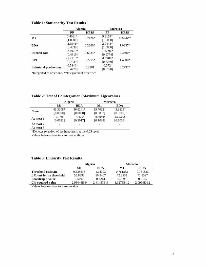
4. Test Results We have two stationarity tests, the PP test (Phillips & Perron, 1988) and the KPSS test (Kwiatkowski, Phillips, Schmidt & Shin, 1992). The first test allows us to test for the unit root hypothesis. The second is used for testing the stationarity hypothesis. The use of these

7

two tests permits us to distinguish stationary from non stationary series, and also gives us an idea on the series whose data do not provide enough information on the stationarity. Test results of the stationarity are presented in Table (1). According to these results, and except for the M1 for Morocco, all the variables are integrated of order I (using the two tests). For the above mentioned variables, the PP and the KPSS tests did not render the same results. Thus, we have opted for the PP test, and consequently the variables are integrated of order I (i.e. I(1)).

Since all the variables are I(1) series, we proceed using the cointegration test Johansen & Juselius (1990). The test results are presented in Table (2).

The cointegration tests were performed using the two proxies of monetary policy in order to see if changing the proxy could have an impact on the nature of the variables’ relationships.

Test results in Table (2) show that cointegration relationships exist between the variables no matter what proxy of monetary policy is used.

After conducting stationarity and cointegration tests, we proceed to carry a linearity test as proposed by Tsay (1998). This test will permit us to choose between using a VAR model or an MVTAR model for the estimation of the response functions. According to the results presented in Table (3), a nonlinear relationship exists in the case of Morocco, which supports using an MVTAR model. In the case of Algeria, the results are in favor of using a VAR model.

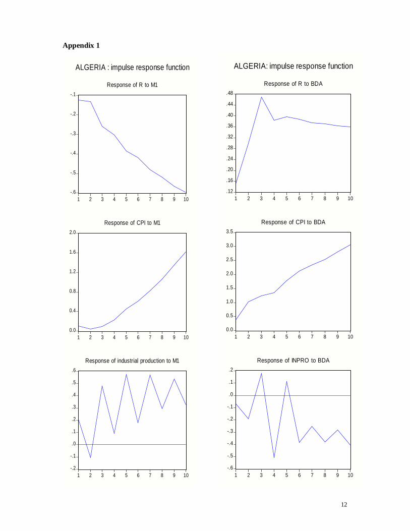
The results of the response functions based on VAR models for the case of Algeria are presented in Appendix 1.

Appendix 1 shows that the interest rate has a negative response which tends to decrease without return to equilibrium when facing an M1 shock. Thus, this could be interpreted by a high liquidity effect of M1. When changing the proxy of monetary policy, the results are, however, different. When using the BDA, there is a positive response of the interest rate that tends to increase until the 3rd period, and then decrease to reach the equilibrium in the 4th period. This result reveals a positive relationship in the short term between BDA and the interest rate, and thus the absence of the liquidity effect. In sum, and for the case of Algeria, the M1 has a very strong liquidity effect, unlike other proxies of monetary policy.

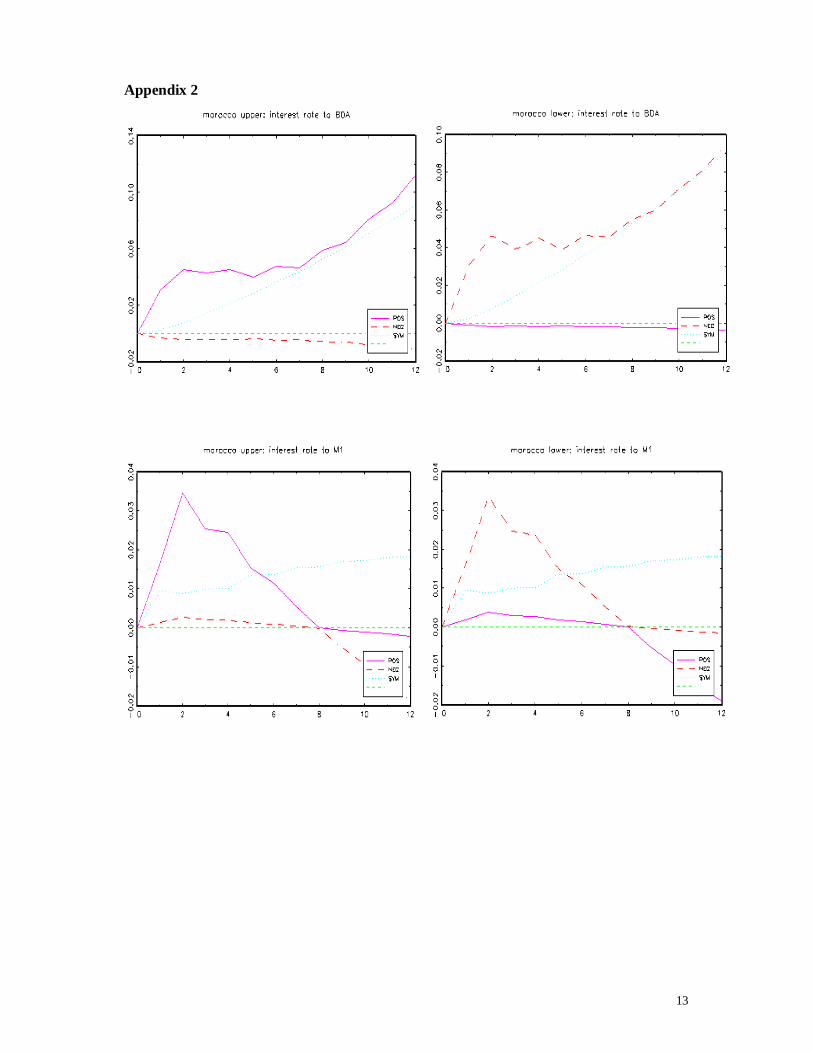
For Morocco, the nonlinear relationship between variables led us to use the generalized response functions based on the MVTAR model. The results of these response functions are presented in Appendix 2. These results can be divided into two parts: the upper regime and the lower regime. The upper regime is characterized by a high inflation whereas the lower regime is dominated by a low rate of inflation. For the upper regime, using M1, we see a positive response from the interest rate that tends to increase until the second period and then decreased till the 8th period where it vanishes. After the 8th period, there is a negative response that tends to decrease at a low speed. By changing the proxy from M1 to BDA, we get a different result. This result is characterized by a positive response which tends to increase continuously. Thus, this can be interpreted by the absence of the liquidity effect for the two proxies used, despite the negative response of low interest rates after the eighth period when using M1.

For the lower regime, and using M1, the result is almost similar except that the speed of change of the positive responses has weakened, and the speed of change of negative responses has increased, which might be in favor of the liquidity effect. When using the proxy BDA, however, there is a clear negative response that tends to decrease at a low speed.

8

Thus, this negative response reflects a negative relationship between the BDA and the interest rate, which can be interpreted by the existence of a liquidity effect. This result in the case of Morocco corresponds well with those of Shen C. H. and C-N. Chiang (1999). Indeed, using the MVTAR model we were able to split the economy into two regimes — high and low inflation regimes. During high inflation periods, the anticipated inflation effect dominates3 throughout the period, whereas the liquidity effect dominates during low inflation periods.

In addition, this liquidity effect is better detected using a proxy other than M1 for monetary policy. This is consistent with the literature which postulates that the liquidity effect disappears when using M1 as a proxy of monetary policy (Leeper and Gordon, 1992 ; Christiano and Eichenbaum, 1992).

5. Conclusion In this paper, our main concern is testing for the liquidity effect in Algeria and Morocco. In order to consolidate our approach, an MVTAR as proposed by Tsay (1998) is used. If the VAR has a nonlinear threshold relationship, it is necessary to differentiate the regime based on a threshold level of the switching variable. Thus, assuming that the latter is the rate of inflation, the MVTAR allows us to subdivide data into low and high inflation regimes. The literature indicates that the existence of the liquidity effect depends on the proxy used to represent monetary policy. No liquidity effect is detected if monetary policy is measured by M1 (Leeper and Gordon (1992); Christiano and Eichenbaum (1992)], whereas a liquidity effect may be detected if the NBR is employed (Christiano and Eichenbaum (1992); Strongin (1995)). However, due to the absence of NBR data in the Maghreb countries, we have proposed another proxy for monetary policy, namely the BDA. Our results do not support threshold behavior in the case of Algeria. Moreover, when using M1 as a proxy of monetary policy, the liquidity effect hypothesis is rejected in this country. When using BDA, results show that there is a negative relationship between monetary shocks and interest rate, and accordingly accepting the liquidity effect. Secondly, in the case of Morocco, however, results show an asymmetric response of interest rate to positive and negative shocks of monetary policy. Moreover, these results strongly support a threshold behavior when BDA is employed, while weakly supporting the same behavior when using M1. Furthermore, using the proxy of BDA, the liquidity effect is accepted in the low inflation regime, whereas it is rejected in the high inflation regime. Hence, the threshold behavior offers an interesting alternative for explaining the relationship between interest rates and monetary policy shocks.

The results presented herein may give more insights on the transmission mechanism of monetary policy in different inflationary environments. Accordingly, a good inflation targeting policy would yield better results in this context. Indeed, the liquidity effect breaks down for the high inflation regime, as inflationary expectations are immediately responsive to money growth. In a low inflation regime, however, money is not considered to be neutral, as it could affect output through the liquidity effect.

3 The comparison between the liquidity effect and the anticipated inflation effect is already used in Cochrane J. H. (1989) “I present evidence of a negative short-run correlation between money growth and interest rates, which I interpret as evidence that the liquidity effect dominates the anticipated inflation effect”.

9

References: Astanasova, C. 2003. “Credit Market Imperfections and Business Cycle Dynamics: A

Nonlinear Approach”. Studies in Nonlinear Dynamics & Econometrics 7(4), article 5.

Beaudry, Paul and Gary Koop. 1993. “Do Recessions Permanently Change Output?” Journal of Monetary Economics, Vol. 31, N. 2, pp 149-163, April.

Bernanke, B. S. 1998. “The Liquidity Effect and Long-Run Neutrality”. Carnegie-Rochester Conference Series on Public Policy 49, 149–194.

Bernanke, B. S. and A. S. Blinder. 1992. “The Federal Funds Rate and the Channels of Monetary Transmission”. The American Economic Review Vol. 82, N°.4, pp. 901-921.

Bilan, O. 2005. “In Search of the Liquidity Effect in Ukraine”. Journal of Comparative Economics 33, pp. 500–516.

Cagan, Philip. 1972. "Introduction to "The Channels of Monetary Effects on Interest Rates" NBER Chapters, in: The Channels of Monetary Effects on Interest Rates, pages 1-8 National Bureau of Economic Research, Inc.

Chan, K.S. 1993. “Consistency and Limiting Distribution of the Least Squares Estimator of a Threshold Autoregressive Model”. The Annals of Statistics 21, 520–533.

Chen S. –L, L. –J Tsai, and J. –L Wu. 2004. “A Revisit to Liquidity Effect: Evidence from a Non-Linear Approach”. Journal of Macroeconomics (26), pp. 501–517.

Christiano, L. J. and M. Eichembaum. 1992a. “Liquidity Effects, Monetary Policy, and the Business Cycle”. Discussion Paper 70. Institute for Empirical Macroeconomics, Federal Reserve Bank of Minneapolis.

Christiano, L. J. and M. Eichenbaum. 1992b. “Liquidity Effect and the Monetary Transmission Mechanism”. The American Economic Review Vol. 82, N°. 2, pp. 346–353.

Christiano, L. J., Eichenbaum, M., and C. Evans. 1994. “The Effect of Monetary Shocks: Evidence from the Flow of Funds”. NBER working paper No. 4699.

Cochrane, J. H. 1989. “The Return of the Liquidity Effect: A Case Study of the Short-Run Relation between Money Growth and Interest Rates”. Journal of Business & Economic Statistic Vol. 7, N°. 1, pp. 75–83.

Friedman, M. 1968. “The Role of Monetary Policy”. American Economic Review 58, 1–17.

Gali, J. 1998. “The Liquidity Effect and Long-Run Neutrality: A Comment”. Carnegie-Rochester Conference Series on Public Policy 49, 195–206.

Guirguis, H. S. 1999. “Properly Estimating the Liquidity Effect: Why Accounting for Stationarity and Outliers Is Important”. Journal of Economics and Business 51, 303–314.

Hansen, Bruce E. 1996. “Estimation of VAR Models”. Working papers in economics 325. Boston College Department of Economics.

Johansen, S. and K. Juselius. 1990. “Maximum Likelihood Estimation and Inference on Cointegration: With Applications to the Demand for Money”. Oxford Bulletin of Economics and Statistics 52 (2): 169–210.

Koop, G., M. H. Pesaran and M. Potter. 1996. “Impulse Response Analysis in Nonlinear Multivariate Models”. Journal of Econometrics 74, 119–147.

10

Kwiatkowski, D., Phillips C.B., Schmidt, P. and Y. Shin. 1992. “Testing the Null Hypothesis of Stationary against the Alternative of A Unit Root”. Journal of Econometrics 54, 159– 178.

Leeper, E. M., and D. B. Gordon. 1992. “In Search of the Liquidity Effect”. Journal of Monetary Economics 29(3):341–369. June.

Mishkin, F. S. 1982. “Does Anticipated Monetary Policy Matter? An Econometric Investigation”. Journal of Political Economy 90, 22–51.

Normandin, M., and L. Phaneuf. 1996. “The Liquidity Effect: Testing Identification Conditions Under Time-Varying Conditional Volatility”. working paper 40. Cahier de Recherche.

Phillips, P.C.B. and P. Perron. 1988. “Testing for a Unit Root in Time Series Regression”. Biometrika 75 (2): 335– 346.

Reichenstein, W. Jan. 1987. “The Impact of Money on Short-Term Interest Rates”. Economic Inquiry 25, 67–82.

Shen, C. H. and C-N. Chiang. 1999. “Retrieving the Vanishing Liquidity Effect: A Threshold Vector Autoregressive Model”. Journal of Economics and Business 51, 259–277.

Sims, C. A. 1992. “Interpreting the Macroeconomic Time Series Facts: The Effect of Monetary Policy”. European Economic Review 36, 975–1000.

Strongin, S. 1995. “The Identification of Monetary Policy Disturbances Explaining the Liquidity Puzzle”. Journal of Monetary Economics 35, 463–497.

Thornton, D. L. 2001. “The Federal Reserve’s Operating Procedure, Non-Borrowed Reserves, Borrowed Reserves and the Liquidity Effect”. Journal of Banking & Finance 25, 1717–1739.

Tsay, Ruey S. 1998. “Testing and Modeling Multivariate Threshold Models”. Journal of the American Statistical Association. Vol. 93, N°. 443, pp. 1188–1202.

Weise, C. L. 1999. “The Asymmetric Effects of Monetary Policy: A Nonlinear Vector Autoregression Approach”. Journal of Money, Credit and Banking. Vol. 31, N°. 1, pp. 85–108.

11

Table 1: Stationarity Test Results

Algeria Morocco PP KPSS PP KPSS

M1 2.4031* [1.0000] 0.2426* 9.3159*

[1.0000] 0.3426**

BDA -2.1941* [0.4839] 0.2366* 2.0448*

[1.0000] 1.0337*

Interest rate -2.1979* [0.4819] 0.6923* -0.5994*

[0.9774] 0.3590*

CPI -1.7116* [0.7339] 0.2215* -1.7480*

[0.7249] 1.4800*

Industrial production -0.5446* [0.4770] 0.2201 -0.5724

[0.8720] 0.2797*

*Integrated of order one, **Integrated of order two Table 2: Test of Cointegration (Maximum Eigenvalue)

Algeria Morocco M1 BDA M1 BDA

None 43.3208* [0.0000]

56.6241* [0.0000]

35.7032* [0.0037]

45.3824* [0.0007]

At most 1 17.1599 [0.0621]

13.4255 [0.2017]

18.6050 [0.1088]

23.2332 [0.1059]

At most 2 - - - - At most 3 - - - - *Denotes rejection of the hypothesis at the 0.05 level. Values between brackets are probabilities. Table 3: Linearity Test Results

Algeria Morocco M1 BDA M1 BDA

Threshold estimate 0.635533 1.14393 0.761833 0.761833 LM test for no threshold 55.8998 56.3467 72.8502 71.8527 Bootstrap p-value 0.5197 0.3244 0.0095 0.0165 Chi squared value 2.95046E-9 2.41457E-9 1.3276E-12 2.0999E-12 Values between brackets are p-value.

12

Appendix 1

-.6

-.5

-.4

-.3

-.2

-.1

1 2 3 4 5 6 7 8 9 10

Response of R to M1

0.0

0.4

0.8

1.2

1.6

2.0

1 2 3 4 5 6 7 8 9 10

Response of CPI to M1

-.2

-.1

.0

.1

.2

.3

.4

.5

.6

1 2 3 4 5 6 7 8 9 10

Response of industrial production to M1

ALGERIA : impulse response function

.12

.16

.20

.24

.28

.32

.36

.40

.44

.48

1 2 3 4 5 6 7 8 9 10

Response of R to BDA

0.0

0.5

1.0

1.5

2.0

2.5

3.0

3.5

1 2 3 4 5 6 7 8 9 10

Response of CPI to BDA

-.6

-.5

-.4

-.3

-.2

-.1

.0

.1

.2

1 2 3 4 5 6 7 8 9 10

Response of INPRO to BDA

ALGERIA: impulse response function

13

Appendix 2