Download - The interpoint distance distribution as a descriptor of point patterns, with an application to spatial disease clustering

STATISTICS IN MEDICINEStatist. Med. (in press)Published online in Wiley InterScience (www.interscience.wiley.com). DOI: 10.1002/sim.1947

The interpoint distance distribution as a descriptor of pointpatterns, with an application to spatial disease clustering

Marco Bonetti1;2;∗;† and Marcello Pagano1

1Department of Biostatistics; Harvard School of Public Health; Boston; MA 02115; U.S.A.2Dana-Farber Cancer Institute; Boston; MA 02115; U.S.A.

SUMMARY

The topic of this paper is the distribution of the distance between two points distributed independentlyin space. We illustrate the use of this interpoint distance distribution to describe the characteristics ofa set of points within some �xed region. The properties of its sample version, and thus the inferenceabout this function, are discussed both in the discrete and in the continuous setting. We illustrateits use in the detection of spatial clustering by application to a well-known leukaemia data set, andreport on the results of a simulation experiment designed to study the power characteristics of themethods within that study region and in an arti�cial homogenous setting. Copyright ? 2004 John Wiley& Sons, Ltd.

KEY WORDS: distance-based methods; Monte Carlo sampling; U-statistics; disease clusters

1. INTRODUCTION

Consider the distance between two points. If one of the points is �xed and the other random,then we have a non-negative random variable and a large scienti�c literature associated withits study. On the other hand, if both points are random, then the general study of such arandom distance occupies only a rather small part of the statistical literature, and only inthe simpler cases can its distribution be derived analytically (see References [1–4]). To drawinference about such a distribution, one may take a random sample of n points, which resultin the larger (for n¿3) number of

(n2

)dependent distances.

Except for very simple cases, it is very di�cult to analytically express the dependen-cies among these distances. But yet it is informative, and thus desirable, as we show be-low, to study such distributions. Their natural estimator, the empirical frequency distribution

∗Correspondence to: Marco Bonetti, Department of Biostatistics, Harvard School of Public Health, 655 HuntingtonAvenue, Boston, MA 02115, U.S.A.

†E-mail: [email protected]

Contract=grant sponsor: National Institutes of Health; contract=grant numbers: AI28076 and LM07677-01

Received May 2003Copyright ? 2004 John Wiley & Sons, Ltd. Accepted May 2004

M. BONETTI AND M. PAGANO

function (‘ecdf’) of the(n2

)dependent distances, can form the basis for inference. Because

of the dependencies, the study of this estimator does not follow the usual paradigm of anempirical cumulative distribution function based on independent identically distributed(i.i.d.) observations, and thus it is not as straightforward to obtain its samplingproperties.There is a round about way of arriving at this estimator that follows more familiar lines.

Suppose n is even. We can easily obtain n=2 independent distances, and construct theirempirical cdf. There are n!=(2n=2(n=2)!) ways of choosing the n=2 independent distances.To gain e�ciency we can take a resampling approach and average all possible empiricalcdfs based on n=2 independent distances. It is not di�cult to show that with this approachone recovers exactly the frequency distribution of all the dependent distances, the ecdf. Aparallel may be drawn with the calculation of the sample variance S2n of n (even) num-bers X1; : : : ; Xn. Given S2n =(n − 1)−1

∑ni=1(Xi − �Xn)2, with �Xn the sample mean, it is well

known that S2n =(n(n − 1))−1∑n−1

i=1

∑nj=i+1(Xi − Xj)2, an average of dependent quantities.

Considering a random permutation � of the indices i=1; : : : ; n, one can then de�ne the esti-mator S2� = n

−1 ∑n=2i=1(X2i−1−X2i)2, an unbiased but ine�cient estimator based on independent

summands. Then averaging these S2� over all n!=(2n=2(n=2)!) distinct ways of creating inde-

pendent pairs, yields exactly S2n .The ecdf converges to the distribution of the interpoint distance between two randomly

selected observations [3], so that for �nite, but large n, one may compare the ecdf of the(n2

)distances to its population counterpart to evaluate the agreement between the sample and

a hypothesized population distribution. The genesis of the idea to use the interpoint distancedistribution is evident in the work of Bartlett [2], who studies points uniformly distributedwithin a unit circle and a unit square. This approach is applicable to the situation in whichthe points are generated according to an absolutely continuous distribution over a region, aswell as to the situation in which the points are constrained to belong to one of a �xed, andpossibly �nite, set of possibilities.In what follows we will see that the ecdf of all pairwise distances evaluated at a �nite

number of values along the distance axis has an asymptotic multivariate normal distribu-tion. More generally, we also provide a new proof of the result that the centred empiricalfrequency distribution of the pairwise distances converges to a Gaussian process. One canthen evaluate the di�erence between the empirical frequency distribution and its populationcounterpart in a variety of ways. For example, if the ecdf is computed over a �nite grid,then a statistic resembling a Mahalanobis distance can be used to construct a chi-squared-like test statistic. In Section 2, we discuss the interpoint distance distribution both in thecontinuous case and in the discrete case. The initial motivation for our work was the prob-lem of the detection of disease clustering over a population non-uniformly distributed overa region, and in Section 3, we show an application of our methods to that particular settingwith an illustration based on a well-known data set. In Section 4, we describe a simulationstudy of the power of the proposed methods in comparison to some other existing clus-tering statistics. This motivation for our work in�uences the assumptions we make of ourmodels. In general, we view the sampling region as given and �xed, and not as a sampledpart of a larger whole. As a consequence, for inference we eschew such restrictive assump-tions as stationarity of underlying point processes and prefer to turn to exact resamplingmethods.

Copyright ? 2004 John Wiley & Sons, Ltd. Statist. Med. (in press)

THE INTERPOINT DISTANCE DISTRIBUTION

2. THE INTERPOINT DISTANCE DISTRIBUTION

2.1. The continuous case

Consider �rst a point process where the observations can appear anywhere inside somebounded region. Let the point distribution over the region be absolutely continuous, so thatfor two i.i.d. points X1 and X2 in the region, Pr(X1 =X2)=0.For any point distribution P in a region S, on which is de�ned a non-negative distance (or

dissimiliarity) function d, the cdf F(·) of the interpoint distance D between two independentpoints is F(d)=E1(d(X1; X2)6d), where 1(·) is the indicator function and E denotes expec-tation with respect to the P×P distribution. For example, on the plane, Bartlett [2] reports thedistribution of the interpoint distances for randomly distributed points on the unit square andon the unit circle (results originally due to Borel [1]), and he suggests computing a chi-squaretest to measure the deviation between the observed and the expected frequencies over a grid.He also recognizes that distributional problems arise because the observed distances do notconstitute a sample of independent observations.If one views the sampling region as itself a sample of some bigger space, then to extrap-

olate the results beyond the region we require some property of the process to make thisgeneralization reasonable. One such property is that of stationarity. A point process de�nedon a topological space S is said to be stationary if its distribution is invariant under a topo-logical group G acting continuously on S (a typical example being the group G of rigidmotions acting on the plane). The de�nition, and use, of the interpoint distribution functionF(d) given above does not require that the point process be stationary, but if it is, a numberof theoretical results are available. In the setting of stationary isotropic processes, Ripley [5]de�nes the K-function

K(t)= �−1E[number of further events within distance t of an arbitrary event]

where � is the intensity of the process, or the (assumed constant) expected number of eventsper unit of area. Ripley points out that the K-function shares some of the properties of theinterpoint distribution function, even though it is not a distribution function; indeed, K(t)→ ∞as t→ ∞. He proposes an estimator of K(t) that in the case of the unit square is unbiased fort¡1=

√2; i.e. half of the maximum distance observable in the unit square, and has variance

that increases rapidly as t increases. Also, if we de�ne Y (t) to be the number of interpointdistances within a region S which are within t of each other (a non-normalized version of theecdf), then Silverman and Brown [6, 7] prove the weak convergence of Y (t) on [0; t0] whent0 is small relative to the maximal distance in S. Within that small interval, Y (t) convergesto a heterogeneous Poisson process (see also [8, p. 44]).Extending the usual de�nition of an empirical distribution function for random samples, we

de�ne the ecdf of the interpoint distances associated with a random sample X1; : : : ; Xn as

Fn(d)=1n2

n∑i=1

n∑j=11(d(Xi; Xj)6d)

For �xed d, Fn(d) is an example of a V-statistic (see for example Reference [9, p. 172]). Inthe appendix it follows that the scaled distribution of Fn(d) computed at a �nite set of values,d1; : : : ; dm, converges to a multivariate normal distribution as n→ ∞ (see also Reference [3]for an alternate proof).



Silverman [3] further showed that the quantity√n(Fn(d)−F(d)), considered as a stochastic

process indexed by d, converges weakly to a Gaussian process. His proof can be shortenedconsiderably by making use of recent results from the theory of U-processes (see Reference[10]), as shown in the appendix. The ecdf of the set of dependent interpoint distances amongn points in the plane is thus a well-de�ned and behaved summary of a con�guration of points.One characteristic of such a descriptor is its rotational invariance, a property that it shareswith all distance-based statistics.

2.2. The discrete case

Consider now a region within which points (individuals) can arise at any of the �xed locationsl1; : : : ; lk with probabilities p1; : : : ; pk (with

∑kj=1 pj=1). Let the random variable D again

represent the distance between two individuals chosen at random from this population. Let dijbe the distance between locations li and lj. The random variable D thus takes on the valuedij with probability pipj. The distribution function of this non-negative random variable is

F(d)=F(d;p)=k∑i=1

k∑j=1pipj1(dij6d) (1)

Consider a random sample n1; : : : ; nk of individuals over this region, and let n=∑k

i=1 ni.Consider all the

(n2

)distances between the individuals in the sample, and compute the func-

tion Fn(d)=F(d; p), where p=(p1; : : : ; pk) and for i=1; : : : ; k, pi= ni=n. Note how thesede�nitions of F(d;p) and F(d; p) are the discrete analogues of F(d) and Fn(d) given inSection 2.1 for the general continuous case.Since we are interested in the distribution of the distances between individuals, and we do

not wish to make assumptions or inference about the value of the sample size, n, we conditionon it. We can then use the distribution of the distances obtained by choosing samples of sizen at locations li with probabilities pi, i=1; : : : ; k (see Reference [11]) as the null distribution.Then the null hypothesis of random sampling from the population distribution is the hypothesisthat the ni are a multinomial sample with probabilities p=(p1; : : : ; pk). Since the pi arestrongly consistent estimators of the pi (as n→ ∞), for any �xed and real d, F(d; p) is astrongly consistent estimator of F(d;p). A measure of the di�erence between F(d; p) andF(d;p) can thus be used as a gauge of the null hypothesis of spatial randomness.Note that in this discrete setting (as opposed to the continuous case) one can expect the

underlying population distribution to be known at least approximately. Here, also, for a �xedvalue d the empirical cdf F(d; p) has

√n-convergence to E(d(X1; X2)6d). Moreover, the

convergence to a multivariate normal distribution holds when one computes the cdf at the�nite set of values d1; d2; : : : ; dm.

2.3. Test statistics

A large number of standard test statistics can be used to evaluate the distance between Fn(·)and F(·), but the lack of independence between observed distances between individuals pre-cludes the use of standard statistics without using appropriate modi�cations.Just as one does for a histogram, one can de�ne an increasing collection of values d=

{d1; : : : ; dm} over the range of D and de�ne the two vectors Fn(d)= {Fn(d1); : : : ; Fn(dm)} andF(d)= {F(d1); : : : ; F(dm)}.



The asymptotic normality noted in the previous sections suggests the following statistic tomeasure the distance between Fn(d) and F(d):

M (Fn(d); F(d))= (Fn(d)− F(d))′�−(Fn(d)− F(d)) (2)

a Mahalanobis-like statistic, where �− is a generalized inverse (see Reference [12]) of thecovariance matrix of the vector Fn(d). For de�niteness we use the Moore–Penrose generalizedinverse. One can, in theory, compute the exact distribution of M , but if n is of any reasonablesize, the calculation is not feasible. As an alternative, one could appeal to the asymptotic resultsin the appendix, but empirical experience suggests that the convergence of the distribution ofM to its asymptotic value is quite slow. This is especially so in discrete situations where thereare many locations, since then typically a number of the probabilities pi involved are small.Because of this, we do not use M , but rather propose using an estimator of M . Consider Mde�ned as M , but with the estimated covariance matrix

M (Fn(d); F(d))= (Fn(d)− F(d))′S−(Fn(d)− F(d)) (3)

where S is the sample covariance estimator obtained after taking repeated samples, withreplacement, of size n. This is the statistic we propose to use, with the generalized inversematrix S− chosen to be the Moore–Penrose generalized inverse of S. In practice we havesampled repeatedly 1000 times with success.When comparing the sample and theoretical distributions, it is sometimes more instructive

to see the scaled �rst di�erence function fn(d)

fn(d)= 1� [Fn(d+ �=2)− Fn(d− �=2)]

One typically de�nes (and plots) a vector fn(d)= (fn(d1); : : : ; fn(dm)) of values computedat values d1; : : : ; dm taken here to be such that dj − dj−1 = � for j=1; : : : ; m and m somepositive integer. We set d1 = �=2, and de�ne fn(d1)=Fn(�)=� so that it includes the origin.The population equivalent of fn(d) is the vector f(d)= (f(d1); : : : ; f(dm)) computed at thesame values d1; : : : ; dm, but replacing Fn(·) by F(·). Because of its linear relationship withFn(·), the �rst di�erence function fn(·) has

√n-convergence to the expected value E(1(d −

�=2¡d(X1; X2)6d+�=2), and for a �xed d, n1=2fn(d) has an asymptotically normal distribution.The joint asymptotic distribution for multiple values of d also follows immediately.Above we have de�ned the statistic M and M in terms of F(·) and Fn(·), but note that

we could equally well de�ne them in terms of fn(·) and f(·) computed at the same val-ues d=(d1; : : : ; dm). The two forms with, of course, appropriate de�nitional changes in thecovariance matrix, yield identical results. Statistics other than M can be de�ned by choos-ing a di�erent distance measure between fn(·) and f(·). Below we explore the followingpossibilities:

M1(fn; f) =∫ ∞

0(fn(x)− f(x))2 d�(x)

M�2 (fn; f) =∫ ∞

0

(fn(x)− f(x))2f(x)

d�(x)

MKL(fn; f) =∫ ∞

0log

(fn(x)f(x)

)f(x) d�(x)



M1 is the L2 norm of the di�erence between fn and f; M�2 is a �2-type distance; and MKL isthe well-known Kullback–Leibler semi-metric. One method of approximately evaluating theseintegrals is with respect to the discrete measure � that puts equal mass at equispaced pointsat which fn and f are evaluated, so that they become sums. Derivation of the asymptoticdistributions of these statistics is di�cult, but we can again rely on the Monte Carlo samplingapproach to construct tests of hypotheses.

3. AN APPLICATION TO CLUSTER DETECTION

3.1. Disease clustering

The search for clusters in the spatial distribution of a set of points is an important problemwith a long history in statistics. One notable application of methodologies developed in thiscontext is the search for disease clustering, especially in response to alarms raised by thepublic. (See for example Reference [13] and references therein).In their search for such clusters, the Centres for Disease Control and Prevention in

Atlanta have issued cluster detection guidelines that contain the rather pessimistic statementthat ‘in many reports of cluster investigations, a geographic or temporal excess in the numberof cases cannot be demonstrated’ [14]. This guarded view may be the result of the ratherpoor success rate in cluster detections (out of 108 suspected cancer clusters investigated over22 years, no clear cause was found for any of them; see Reference [15]), although this couldmean either that false alarms are raised too easily (alarms that under further study are readilydismissed), or that existing methods are not su�ciently powerful for detecting clusters. Someof the existing clustering methods are reviewed in Reference [16], where one can also �nd adescription of many model-based approaches aimed at assessing dependence in spatial pointprocesses.We can use the methods described here to test whether the observed interpoint distance

distribution among the individuals with a certain disease is consistent with the hypothesis ofno disease-induced clustering. It should be noted that these methods are designed to detect anydisturbance from such distribution, and not just a single cluster. This can be quite important,since in most cases one does not know the number, shape and location of the clusters thatmay exist. In this section we discuss the discrete case, because the application that followsis discrete, as it is in many cluster investigations since the data typically is only availablein aggregate form; either because of the data collection method or because of concerns forcon�dentiality.For a given set of �xed centres, the lack of deviations from the population distribution is

equivalent to choosing as cases of the disease of interest individuals, at random, from thecentres, with probabilities given by the appropriate population proportions: pi, i=1; : : : ; k.So when we consider a group of individuals with a particular ailment (leukaemia, say), andask whether they are geographically distributed as in the population—the null hypothesis ofno clustering—then we immediately think of the goodness-of-�t problem, and the associatedclassical chi-squared test for the multinomial distribution. This test is a general one and is nottargeted at the clustering problem at hand. Indeed, we can think of the chi-squared goodness-of-�t test as a quadratic form (p−p)′�−(p−p) involving the di�erence between the observed(p) and expected (p) proportions, where the weighting matrix �− is the generalized inverse



Interpoint distance

0 50 100 150

0.00

0.25

0.50

0.75

1.00

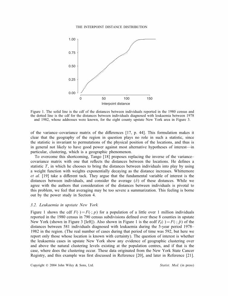
Figure 1. The solid line is the cdf of the distances between individuals reported in the 1980 census andthe dotted line is the cdf for the distances between individuals diagnosed with leukaemia between 1978and 1982, whose addresses were known, for the eight county upstate New York area in Figure 3.

of the variance–covariance matrix of the di�erences [17, p. 44]. This formulation makes itclear that the geography of the region in question plays no role in such a statistic, sincethe statistic is invariant to permutations of the physical position of the locations, and thus isin general not likely to have good power against most alternative hypotheses of interest—inparticular, clustering, which is a geographic phenomenon.To overcome this shortcoming, Tango [18] proposes replacing the inverse of the variance–

covariance matrix with one that re�ects the distances between the locations. He de�nes astatistic T , in which he chooses to bring the distances between individuals into play by usinga weight function with weights exponentially decaying as the distance increases. Whittemoreet al. [19] take a di�erent tack. They argue that the fundamental variable of interest is thedistances between individuals, and consider the average (�) of these distances. While weagree with the authors that consideration of the distances between individuals is pivotal tothis problem, we feel that averaging may be too severe a summarization. This feeling is borneout by the power study in Section 4.

3.2. Leukaemia in upstate New York

Figure 1 shows the cdf F(·)=F(·;p) for a population of a little over 1 million individualsreported in the 1980 census in 790 census subdivisions de�ned over these 8 counties in upstateNew York (shown in Figure 3 [left]). Also shown in Figure 1 is the ecdf Fn(·)=F(·; p) of thedistances between 581 individuals diagnosed with leukaemia during the 5-year period 1978–1982 in the region. (The real number of cases during that period of time was 592, but here wereport only those whose location is known with certainty). The question of interest is whetherthe leukaemia cases in upstate New York show any evidence of geographic clustering overand above the natural clustering levels existing at the population centres, and if that is thecase, where does the clustering occur. These data originated from the New York State CancerRegistry, and this example was �rst discussed in Reference [20], and later in Reference [21].



Interpoint distance0 50 100 150

0.000

0.005

0.010

0.015

0.020

0.025

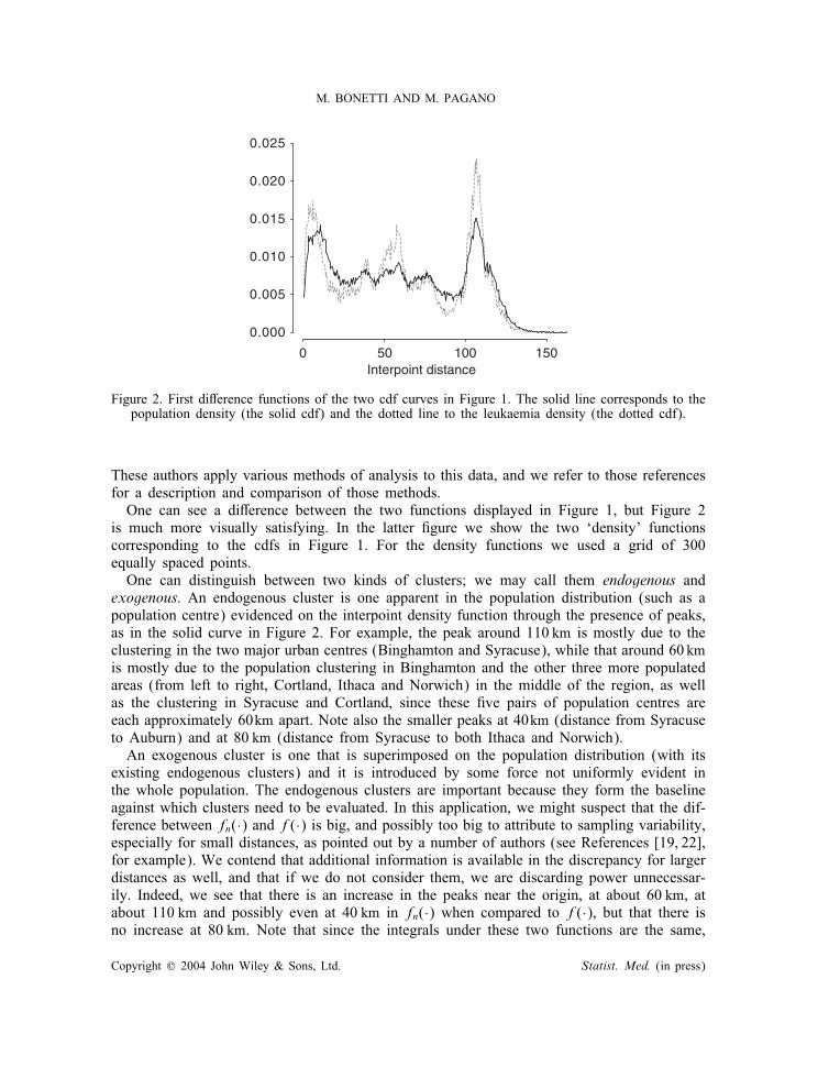
Figure 2. First di�erence functions of the two cdf curves in Figure 1. The solid line corresponds to thepopulation density (the solid cdf) and the dotted line to the leukaemia density (the dotted cdf).

These authors apply various methods of analysis to this data, and we refer to those referencesfor a description and comparison of those methods.One can see a di�erence between the two functions displayed in Figure 1, but Figure 2

is much more visually satisfying. In the latter �gure we show the two ‘density’ functionscorresponding to the cdfs in Figure 1. For the density functions we used a grid of 300equally spaced points.One can distinguish between two kinds of clusters; we may call them endogenous and

exogenous. An endogenous cluster is one apparent in the population distribution (such as apopulation centre) evidenced on the interpoint density function through the presence of peaks,as in the solid curve in Figure 2. For example, the peak around 110 km is mostly due to theclustering in the two major urban centres (Binghamton and Syracuse), while that around 60 kmis mostly due to the population clustering in Binghamton and the other three more populatedareas (from left to right, Cortland, Ithaca and Norwich) in the middle of the region, as wellas the clustering in Syracuse and Cortland, since these �ve pairs of population centres areeach approximately 60km apart. Note also the smaller peaks at 40km (distance from Syracuseto Auburn) and at 80 km (distance from Syracuse to both Ithaca and Norwich).An exogenous cluster is one that is superimposed on the population distribution (with its

existing endogenous clusters) and it is introduced by some force not uniformly evident inthe whole population. The endogenous clusters are important because they form the baselineagainst which clusters need to be evaluated. In this application, we might suspect that the dif-ference between fn(·) and f(·) is big, and possibly too big to attribute to sampling variability,especially for small distances, as pointed out by a number of authors (see References [19, 22],for example). We contend that additional information is available in the discrepancy for largerdistances as well, and that if we do not consider them, we are discarding power unnecessar-ily. Indeed, we see that there is an increase in the peaks near the origin, at about 60 km, atabout 110 km and possibly even at 40 km in fn(·) when compared to f(·), but that there isno increase at 80 km. Note that since the integrals under these two functions are the same,



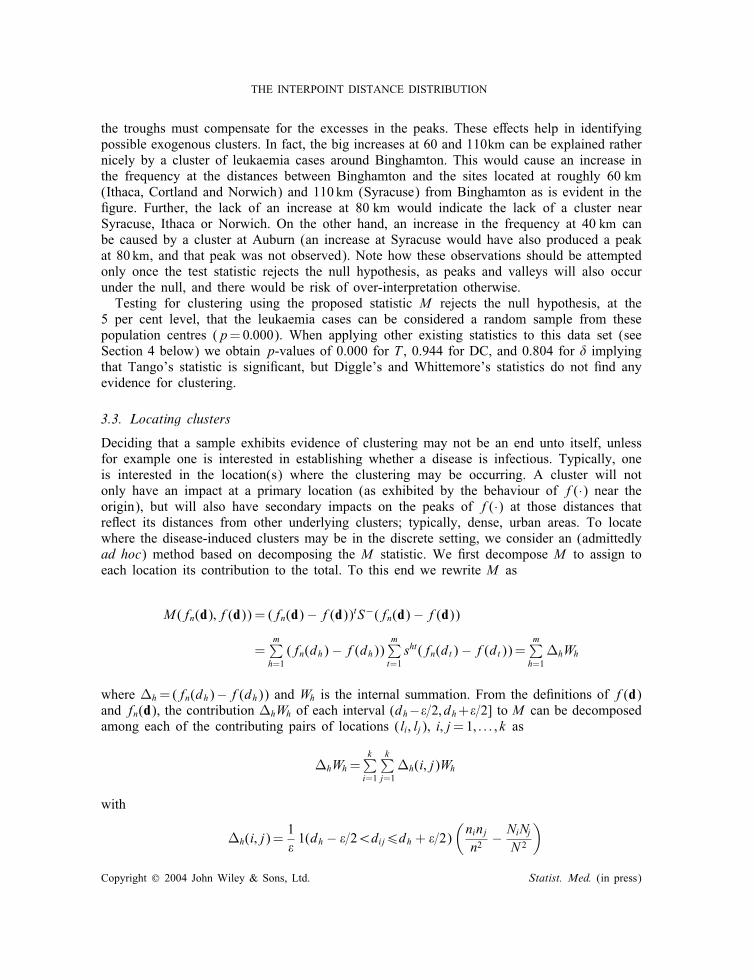
the troughs must compensate for the excesses in the peaks. These e�ects help in identifyingpossible exogenous clusters. In fact, the big increases at 60 and 110km can be explained rathernicely by a cluster of leukaemia cases around Binghamton. This would cause an increase inthe frequency at the distances between Binghamton and the sites located at roughly 60 km(Ithaca, Cortland and Norwich) and 110 km (Syracuse) from Binghamton as is evident in the�gure. Further, the lack of an increase at 80 km would indicate the lack of a cluster nearSyracuse, Ithaca or Norwich. On the other hand, an increase in the frequency at 40 km canbe caused by a cluster at Auburn (an increase at Syracuse would have also produced a peakat 80 km, and that peak was not observed). Note how these observations should be attemptedonly once the test statistic rejects the null hypothesis, as peaks and valleys will also occurunder the null, and there would be risk of over-interpretation otherwise.Testing for clustering using the proposed statistic M rejects the null hypothesis, at the

5 per cent level, that the leukaemia cases can be considered a random sample from thesepopulation centres (p=0:000). When applying other existing statistics to this data set (seeSection 4 below) we obtain p-values of 0.000 for T , 0.944 for DC, and 0.804 for � implyingthat Tango’s statistic is signi�cant, but Diggle’s and Whittemore’s statistics do not �nd anyevidence for clustering.

3.3. Locating clusters

Deciding that a sample exhibits evidence of clustering may not be an end unto itself, unlessfor example one is interested in establishing whether a disease is infectious. Typically, oneis interested in the location(s) where the clustering may be occurring. A cluster will notonly have an impact at a primary location (as exhibited by the behaviour of f(·) near theorigin), but will also have secondary impacts on the peaks of f(·) at those distances thatre�ect its distances from other underlying clusters; typically, dense, urban areas. To locatewhere the disease-induced clusters may be in the discrete setting, we consider an (admittedlyad hoc) method based on decomposing the M statistic. We �rst decompose M to assign toeach location its contribution to the total. To this end we rewrite M as

M (fn(d); f(d)) = (fn(d)− f(d))tS−(fn(d)− f(d))

=m∑h=1(fn(dh)− f(dh))

m∑t=1sht(fn(dt)− f(dt))=

m∑h=1�hWh

where �h=(fn(dh)−f(dh)) and Wh is the internal summation. From the de�nitions of f(d)and fn(d), the contribution �hWh of each interval (dh−�=2; dh+�=2] to M can be decomposedamong each of the contributing pairs of locations (li; lj), i; j=1; : : : ; k as

�hWh=k∑i=1

k∑j=1�h(i; j)Wh

with

�h(i; j)=1�1(dh − �=2¡dij6dh + �=2)

(ninjn2

− NiNjN 2

)



This contribution to the statistic M , �h(i; j)Wh, represents a contribution from two locations,li and lj. How to make the attribution to each of these locations is not unique. We choose toconsider the deviation between the observed proportions (pi= ni=n) and the expected propor-tions (pi=Ni=N ) at those locations. To this end de�ne,

�(i; j)=|pi − pi|

|pi − pi|+ |pj − pj|and assign �(i; j)�h(i; j)Wh and (1 − �(i; j))�h(i; j)Wh to li and lj, respectively. For each ofthe intervals (dh − �=2; dh + �=2] for h=1; 2; : : : ; m, one can then de�ne for each location li atotal contribution to M (or ‘score’) equal to

Score(i)=m∑h=1

k∑j=1�(i; j)�h(i; j)Wh

It is easy to verify that∑k

i=1 Score(i)=M , so that the scores decompose M . Note how thisdecomposition approach is similar in spirit to the examination of local statistics in the analysisof spatial autocorrelation (see References [23–25]).The locations can then be ranked according to their score. In a particular data set, if the

M statistic is signi�cantly di�erent from what would be expected under the null hypothesis,then the locations can be studied to see which locations impact M the most. One strategyfor identifying locations with large contributions to M may be to consider the di�erencebetween the observed value of M and the cut-o� M ∗ corresponding to the test, and �nd theminimum number of locations (having the largest scores) such that the sum of their scoresequals M −M ∗.Application of this procedure yields the map on the right in Figure 3. In the �gure, we

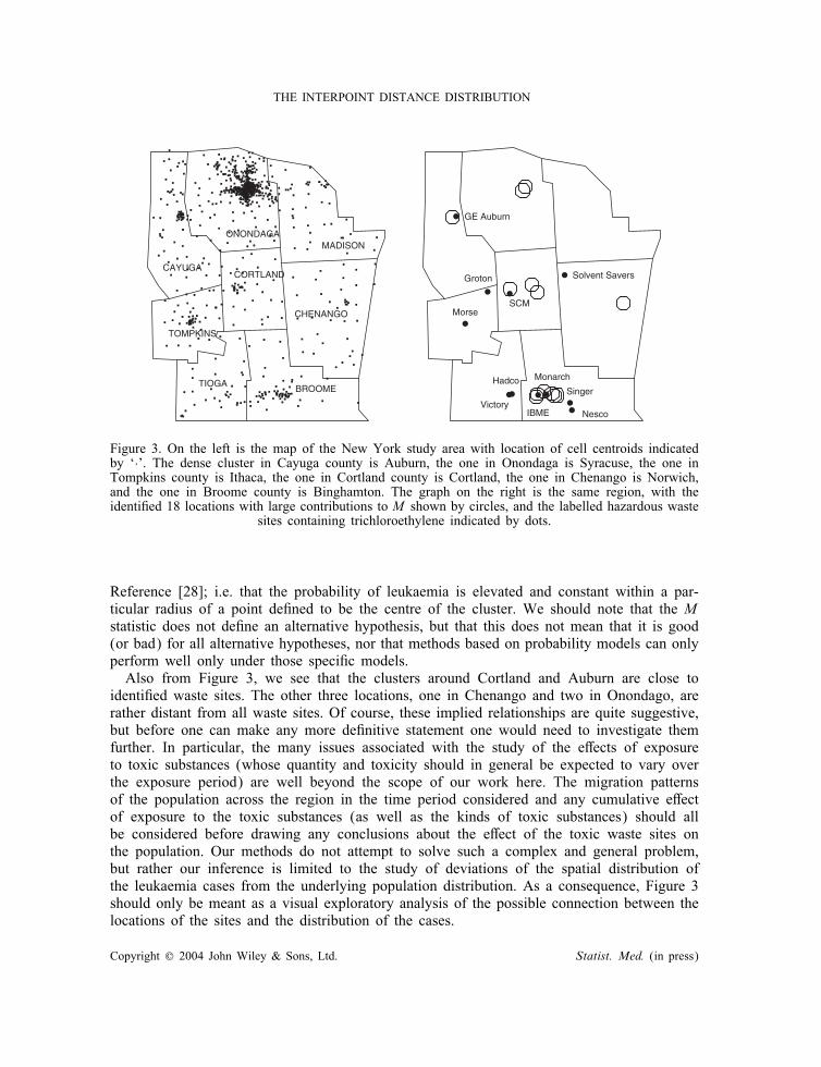
highlight the top 13 locations selected. Even though the interpretation of the results of thecluster localization procedure is perhaps a bit beyond the scope of the proposed tests (andshould therefore be taken with caution), the locations selected can be seen to be suspiciouslyclose to some of the waste sites shown on the map. The number of locations to plot waschosen based on the fact that the di�erence between the observed value of M (144.1) andthe cut-o� point for the corresponding 5 per cent sampling test (44.6) is roughly equal tothe sum of the scores of the top 13 locations (99.7). All of these locations show an excessin the number of leukaemia cases. To ensure stability of the estimated distribution of M wehave used 32 bins for the calculation of the p-value and for the identi�cation of suspiciouslocations. However, a p-value equal to zero and a �gure very similar to Figure 3 wereobtained when using 300 bins in the de�nition of M .Consistent with the impression gained by contrasting fn(·) with f(·), there is an indication

that the locations around Binghamton form a cluster of locations with excess numbers ofleukaemia cases. The locations so identi�ed follow the �ow of the Susquehanna river throughthat region. Two other areas identi�ed are in the upper-left corner and in the middle of themap. These regions were also identi�ed in Reference [20] using the geographical analysis ma-chine method [26] designed for �nding areas with high rates. Unfortunately, the latter methoddoes not lead to a quantitative assessment of the signi�cance of the observed pattern, so thatit is hard to interpret its results. The possibility of clustering of cases around Binghamtonwas also indicated in Reference [27], where the hypothesis of randomness was also rejected.Their likelihood-based approach is constructed on the alternative ‘hot-spot’ model de�ned in



..................

..

.

.. ..... .

................. ........ .

.

..

..

.......

.

...... .... ................... ...

. ........

...

.

..

. . . .. ... .....

...

.......

. . . ........

.... ....

..........

..

....

. .

.. ..

........... ... ....

..

........

. ............

......

.......

....... .

.....

..

.....................................................................................................................................................................................................

........... ................................... ............... .......... .....

. .....

. ... ... ................... ......................... ............................ ............................ ........... ......

.........

...

.......

. .................

......

. ...

.. .....

. ....

.

.

..... ...

....... ...

..

... ....

...........

.. . . ................... . ..

.

. ..........

..

CAYUGA

ONONDAGAMADISON

TOMPKINS

CORTLAND

CHENANGO

TIOGABROOME •• ••

•

••

••

•

•

Monarch

IBME

Singer

Nesco

GE Auburn

Solvent Savers

SCM

Victory

Hadco

Morse

Groton

Figure 3. On the left is the map of the New York study area with location of cell centroids indicatedby ‘·’. The dense cluster in Cayuga county is Auburn, the one in Onondaga is Syracuse, the one inTompkins county is Ithaca, the one in Cortland county is Cortland, the one in Chenango is Norwich,and the one in Broome county is Binghamton. The graph on the right is the same region, with theidenti�ed 18 locations with large contributions to M shown by circles, and the labelled hazardous waste

sites containing trichloroethylene indicated by dots.

Reference [28]; i.e. that the probability of leukaemia is elevated and constant within a par-ticular radius of a point de�ned to be the centre of the cluster. We should note that the Mstatistic does not de�ne an alternative hypothesis, but that this does not mean that it is good(or bad) for all alternative hypotheses, nor that methods based on probability models can onlyperform well only under those speci�c models.Also from Figure 3, we see that the clusters around Cortland and Auburn are close to

identi�ed waste sites. The other three locations, one in Chenango and two in Onondago, arerather distant from all waste sites. Of course, these implied relationships are quite suggestive,but before one can make any more de�nitive statement one would need to investigate themfurther. In particular, the many issues associated with the study of the e�ects of exposureto toxic substances (whose quantity and toxicity should in general be expected to vary overthe exposure period) are well beyond the scope of our work here. The migration patternsof the population across the region in the time period considered and any cumulative e�ectof exposure to the toxic substances (as well as the kinds of toxic substances) should allbe considered before drawing any conclusions about the e�ect of the toxic waste sites onthe population. Our methods do not attempt to solve such a complex and general problem,but rather our inference is limited to the study of deviations of the spatial distribution ofthe leukaemia cases from the underlying population distribution. As a consequence, Figure 3should only be meant as a visual exploratory analysis of the possible connection between thelocations of the sites and the distribution of the cases.



It is of interest to note that only two of the many locations in and around Syracuse (427locations within a radius of 20 km from the centre of Syracuse) are identi�ed as havingexcessive numbers of individuals with leukaemia, even though over 40 per cent of the region’spopulation lives there. Thus the proposed method seems to show considerable speci�city inthis example.

4. A SIMULATION STUDY

We performed a power study to compare the proposed statistics M , M1, M�2 , and MKL de�nedin Section 2.3 with three well-known currently available and easily implementable alternativestatistics: the � statistic [19], the T statistic [18], and the DC statistic [22] based on Ripley’sK-functions. The statistic DC was designed under the assumption of a Cox process, i.e. thatthe underlying distribution be a realization of a Poisson point process having as intensity therealization of a further probability distribution. This implies that the ni should be zeroes orones, but this constraint is usually ignored in application, and we continue in the same veinto use DC both in the discrete and in the continuous setting.Whittemore and colleagues [19] derive the �rst two moments of the � statistic and prove its

asymptotic normality, but rather than rely on this asymptotic result we sample from the exactdistribution since this would yield more accurate results. We do the same for the T statistic.For the DC statistic we use a ratio of 2 to 1 for the number of controls to the number ofcases.We consider two settings: �rst, the situation where points are distributed uniformly over

the unit square; and second, the common situation of �xed locations over a highly non-homogeneous map (the New York State map described in Section 3.2) with more than oneindividual at each location.

4.1. Continuous homogeneous setting

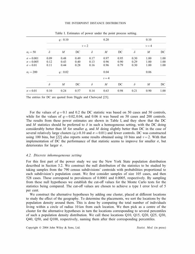
We test the performance of the statistics under the homogeneous point process setting �rstproposed in Reference [29], and also discussed in Reference [22]. We follow the instruc-tions for the simulation in Reference [22], as best we can, to generate the powers for theother statistics, and quote these authors for the power results of their statistic (their esti-mates are based on 100 simulations, ours on 1000). Under the null distribution a sample ofn1 = 50 points is generated uniformly on the unit square, while under the various alternatives(identi�ed by the parameters q, �, and ) some 50q� of these points are deleted and replacedby 50q clusters of � cases, with centres distributed completely at random and cluster mem-bers displaced independently from their corresponding cluster centre according to an isotropicbivariate normal distribution with standard deviation in either co-ordinate direction—thuswith probability one no two points fall in the same location. We computed the power for �and M (with m=20, see Section 2.3) under some of the parameter combinations reported inReference [22]. For the remaining parameter combinations we could not reconstruct the exactalgorithm used to generate the samples as reported in that article since 50q� is not an integer.Note that Tango’s T cannot be used immediately in this setting, so that it does not appear inthe table below.



Table I. Estimates of power under the point process setting.

q : 0:10 0.20 0.10

�=2 �=4

n2 = 50 � M DC � M DC � M DC

=0:001 0.09 0.48 0.49 0.17 0.97 0.95 0.30 1.00 1.00=0:005 0.12 0.43 0.40 0.13 0.96 0.90 0.29 1.00 1.00=0:01 0.11 0.44 0.28 0.16 0.96 0.79 0.30 1.00 1.00

n2 = 200 q : 0:02 0.04 0.06

�=4

� M DC � M DC � M DC

=0:01 0.10 0.24 0.57 0.14 0.63 0.98 0.21 0.90 1.00

The entries for DC are quoted from Diggle and Chetwynd [23].

For the values of q=0:1 and 0.2 the DC statistic was based on 50 cases and 50 controls,while for the values of q=0:02; 0:04, and 0.06 it was based on 50 cases and 200 controls.The results from these power estimates are shown in Table I, and they show that the DCand M statistics should be preferred to � in such a homogeneous setting, with the DC doingconsiderably better than M for smaller q, and M doing slightly better than DC in the case ofseveral relatively large clusters (q¿0:10 and =0:01) and fewer controls. DC was constructedusing 100 bins, but [22] also reports some results obtained using 10 bins and �=2. With thatimplementation of DC the performance of that statistic seems to improve for smaller , butdeteriorates for larger .

4.2. Discrete inhomogeneous setting

For this �rst part of the power study we use the New York State population distributiondescribed in Section 3.2. We construct the null distribution of the statistics to be studied bytaking samples from the 790 census subdivisions’ centroids with probabilities proportional toeach subdivision’s population count. We �rst consider samples of size 105 cases, and then528 cases. These correspond to prevalences of 0.0001 and 0.0005, respectively. By samplingfrom these null hypotheses we establish the cut-o� values for the Monte Carlo tests for thestatistics being compared. The cut-o� values are chosen to achieve a type I error level of 5per cent.We construct the alternative hypotheses by adding one cluster, placed at di�erent locations

to study the e�ect of the geography. To determine the placements, we sort the locations by thepopulation density around them. This is done by computing the total number of individualsliving within a circle of radius 10 km from each location. We then pick as a centre of thecluster for the alternative hypotheses in turn the locations corresponding to several percentilesof such a population density distribution. We call these locations Q10, Q15, Q20, Q25, Q30,Q40, Q50, and Q100, respectively, naming them after their corresponding percentiles.



All deciles between the median and the largest value correspond to locations within oraround Syracuse, and they yield results similar to Q100 (that we label ‘C’ in Table II). Sincewe want a broader representation, we also hand-pick two more locations as positions forthe cluster centre. These locations are in the middle of Auburn (‘A’) and Binghamton (‘B’)respectively, chosen as representatives of small and medium-sized urban centres. Binghamtonis also chosen because of the interest in the potentially hazardous waste sites near that city.We saw in the previous section that the region around Binghamton is identi�ed as a possiblelocation of a cluster of leukaemia cases.To study the extent of the in�uence of a cluster, a radius, , around the cluster centre

is chosen within which the probability of becoming diseased is elevated. We choose threevalues: =2, 5, and 10 km to indicate clusters with increasing impact. Within the radius ofin�uence, we choose a factor � by which to increase the probability of becoming diseased.At the centre of the cluster, the probability of becoming diseased is multiplied by (1 + �),and the increase-factor decreases linearly to one at the perimeter of the circle of radius .(The probabilities are re-scaled to add to one). We choose di�erent values �, as shown inTable I. This is an example of a ‘clinal’ (or ‘conic’) cluster as de�ned in Reference [28].We also study ‘cylindric’ clusters, i.e. clusters for which the same factor (1+�) is applied

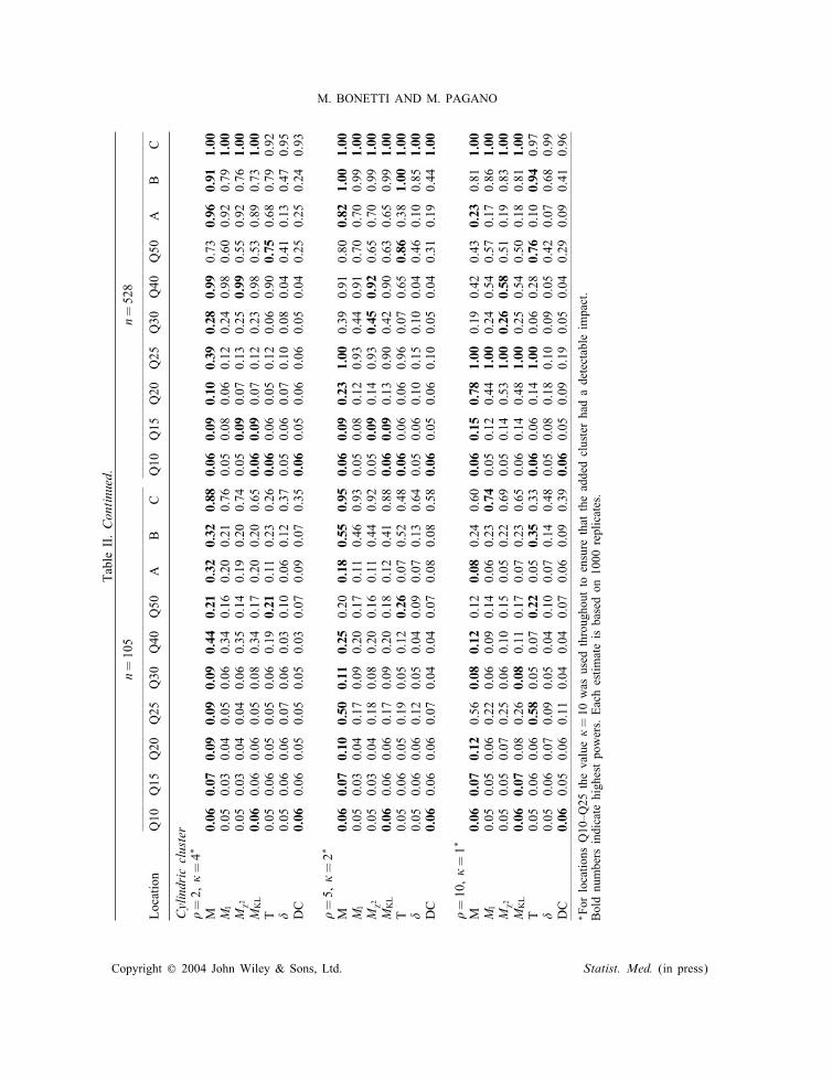
to all locations falling within the cluster, irrespectively of their distance from the centre of thecluster. Among cylindric clusters we experiment with elliptically shaped clusters with ratiosbetween the longest and the shortest diameter in turn equal to 1, 2.5, and 5. These clustersall have their smallest diameter equal to 4 km, so that they are uniquely identi�ed as having equal to 2, 5, and 10 km, respectively.The powers of the statistics are estimated by counting the proportion of the samples (gen-

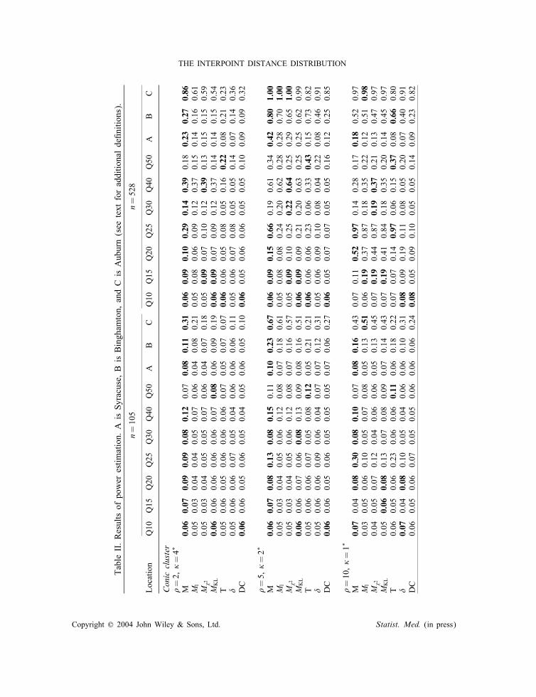
erated according to some alternative hypothesis) that are more extreme than the 5 per centcut-o� values obtained from the null distribution. The way in which we create the alternativehypotheses is such that putting a cluster on a densely populated area will have a strongerimpact on the overall distribution of the cases than a cluster placed on an area of low popula-tion density, since we condition on the total number of cases. This way of creating alternativehypotheses thus makes clusters placed in highly populated areas easier to detect, and givesan overall impression of varying prevalence.Table II shows that the power of all statistics varies with the location of the cluster centre,

its extent (), and the overall prevalence. The power of any statistic in general depends verystrongly on the underlying population distribution as well as on all these parameters, but itseems clear that the proposed statistics M1, M�2 , MKL and M perform very well, and that inparticular the power gain of M over all the other statistics is large. This is probably due to thefact that M is the only one among these statistics that explicitly accounts for the covariancestructure in fn(d). Tango’s T statistic performs quite well, especially when the cluster is placedin highly populated areas such as Q50 and B (in which cases it sometimes even outperformsall other statistics). Quite often, however, its power is much smaller than M ’s. Notice that wechoose the parameter � in the expression of T to be equal to 5, thus making bene�cial use ofprior information (external to the data) about the alternative hypotheses. That information isnot usually available. In fact, expanding exp(−d=5) to the linear term gives 1−d=5, so that Tgives most weight to deviations from the expected counts occurring in the same direction atpairs of locations that are roughly within 5 km of each other. Note that other weight matricescould be de�ned, that take into consideration an assumed spatial structure (see for exampleReference [30]).



TableII.Resultsofpowerestimation.AisSyracuse,BisBinghamton,andCisAuburn(seetextforadditionalde�nitions).

n=105

n=528

Location

Q10

Q15

Q20

Q25

Q30

Q40

Q50

AB

CQ10

Q15

Q20

Q25

Q30

Q40

Q50

AB

C

Coniccluster

=2,�=4∗

M0.06

0.07

0.09

0.09

0.08

0.12

0.07

0.08

0.11

0.31

0.06

0.09

0.10

0.29

0.14

0.39

0.18

0.23

0.27

0.86

M1

0.05

0.03

0.04

0.04

0.05

0.07

0.06

0.04

0.08

0.21

0.05

0.08

0.06

0.09

0.12

0.37

0.15

0.14

0.16

0.61

M�2

0.05

0.03

0.04

0.05

0.05

0.07

0.06

0.04

0.07

0.18

0.05

0.09

0.07

0.10

0.12

0.39

0.13

0.15

0.15

0.59

MKL

0.06

0.06

0.06

0.06

0.06

0.07

0.08

0.06

0.09

0.19

0.06

0.09

0.07

0.09

0.12

0.37

0.14

0.14

0.15

0.54

T0.05

0.06

0.05

0.06

0.06

0.06

0.07

0.05

0.07

0.07

0.06

0.06

0.05

0.08

0.05

0.16

0.22

0.08

0.21

0.23

�0.05

0.06

0.06

0.07

0.05

0.04

0.06

0.06

0.06

0.11

0.05

0.06

0.07

0.08

0.05

0.05

0.14

0.07

0.14

0.36

DC

0.06

0.06

0.05

0.06

0.05

0.04

0.05

0.06

0.05

0.10

0.06

0.05

0.06

0.06

0.05

0.05

0.10

0.09

0.09

0.32

=5,�=2∗

M0.06

0.07

0.08

0.13

0.08

0.15

0.11

0.10

0.23

0.67

0.06

0.09

0.15

0.66

0.19

0.61

0.34

0.42

0.80

1.00

M1

0.05

0.03

0.04

0.05

0.06

0.12

0.08

0.07

0.18

0.61

0.05

0.08

0.08

0.24

0.20

0.62

0.28

0.28

0.70

1.00

M�2

0.05

0.03

0.04

0.05

0.06

0.12

0.08

0.07

0.16

0.57

0.05

0.09

0.10

0.25

0.22

0.64

0.25

0.29

0.65

1.00

MKL

0.06

0.06

0.07

0.06

0.08

0.13

0.09

0.08

0.16

0.51

0.06

0.09

0.09

0.21

0.20

0.63

0.25

0.25

0.62

0.99

T0.05

0.06

0.06

0.07

0.05

0.08

0.12

0.05

0.21

0.21

0.06

0.06

0.06

0.23

0.06

0.33

0.43

0.15

0.73

0.82

�0.05

0.06

0.06

0.09

0.06

0.04

0.07

0.07

0.12

0.31

0.05

0.06

0.09

0.10

0.08

0.04

0.22

0.08

0.46

0.91

DC

0.06

0.06

0.05

0.06

0.05

0.05

0.05

0.07

0.06

0.27

0.06

0.05

0.07

0.07

0.05

0.05

0.16

0.12

0.25

0.85

=10,�=1∗

M0.07

0.04

0.08

0.30

0.08

0.10

0.07

0.08

0.16

0.43

0.07

0.11

0.52

0.97

0.14

0.28

0.17

0.18

0.52

0.97

M1

0.03

0.05

0.06

0.10

0.05

0.07

0.08

0.05

0.13

0.51

0.06

0.19

0.37

0.87

0.18

0.35

0.22

0.12

0.51

0.98

M�2

0.04

0.05

0.07

0.12

0.04

0.06

0.06

0.05

0.13

0.45

0.07

0.19

0.44

0.87

0.19

0.37

0.21

0.13

0.47

0.97

MKL

0.05

0.06

0.08

0.13

0.07

0.08

0.09

0.07

0.14

0.43

0.07

0.19

0.41

0.84

0.18

0.35

0.20

0.14

0.45

0.97

T0.06

0.05

0.06

0.23

0.06

0.06

0.11

0.06

0.18

0.22

0.07

0.07

0.14

0.97

0.06

0.15

0.37

0.08

0.66

0.80

�0.07

0.04

0.08

0.10

0.05

0.04

0.06

0.06

0.10

0.31

0.08

0.09

0.19

0.11

0.08

0.05

0.20

0.07

0.40

0.91

DC

0.06

0.05

0.06

0.07

0.05

0.05

0.06

0.06

0.06

0.24

0.08

0.05

0.09

0.10

0.05

0.05

0.14

0.09

0.23

0.82


M. BONETTI AND M. PAGANOTableII.Continued.

n=105

n=528

Location

Q10

Q15

Q20

Q25

Q30

Q40

Q50

AB

CQ10

Q15

Q20

Q25

Q30

Q40

Q50

AB

C

Cylindriccluster

=2,�=4∗

M0.06

0.07

0.09

0.09

0.09

0.44

0.21

0.32

0.32

0.88

0.06

0.09

0.10

0.39

0.28

0.99

0.73

0.96

0.91

1.00

M1

0.05

0.03

0.04

0.05

0.06

0.34

0.16

0.20

0.21

0.76

0.05

0.08

0.06

0.12

0.24

0.98

0.60

0.92

0.79

1.00

M�2

0.05

0.03

0.04

0.04

0.06

0.35

0.14

0.19

0.20

0.74

0.05

0.09

0.07

0.13

0.25

0.99

0.55

0.92

0.76

1.00

MKL

0.06

0.06

0.06

0.05

0.08

0.34

0.17

0.20

0.20

0.65

0.06

0.09

0.07

0.12

0.23

0.98

0.53

0.89

0.73

1.00

T0.05

0.06

0.05

0.05

0.06

0.19

0.21

0.11

0.23

0.26

0.06

0.06

0.05

0.12

0.06

0.90

0.75

0.68

0.79

0.92

�0.05

0.06

0.06

0.07

0.06

0.03

0.10

0.06

0.12

0.37

0.05

0.06

0.07

0.10

0.08

0.04

0.41

0.13

0.47

0.95

DC

0.06

0.06

0.05

0.05

0.05

0.03

0.07

0.09

0.07

0.35

0.06

0.05

0.06

0.06

0.05

0.04

0.25

0.25

0.24

0.93

=5,�=2∗

M0.06

0.07

0.10

0.50

0.11

0.25

0.20

0.18

0.55

0.95

0.06

0.09

0.23

1.00

0.39

0.91

0.80

0.82

1.00

1.00

M1

0.05

0.03

0.04

0.17

0.09

0.20

0.17

0.11

0.46

0.93

0.05

0.08

0.12

0.93

0.44

0.91

0.70

0.70

0.99

1.00

M�2

0.05

0.03

0.04

0.18

0.08

0.20

0.16

0.11

0.44

0.92

0.05

0.09

0.14

0.93

0.45

0.92

0.65

0.70

0.99

1.00

MKL

0.06

0.06

0.06

0.17

0.09

0.20

0.18

0.12

0.41

0.88

0.06

0.09

0.13

0.90

0.42

0.90

0.63

0.65

0.99

1.00

T0.05

0.06

0.05

0.19

0.05

0.12

0.26

0.07

0.52

0.48

0.06

0.06

0.06

0.96

0.07

0.65

0.86

0.38

1.00

1.00

�0.05

0.06

0.06

0.12

0.05

0.04

0.09

0.07

0.13

0.64

0.05

0.06

0.10

0.15

0.10

0.04

0.46

0.10

0.85

1.00

DC

0.06

0.06

0.06

0.07

0.04

0.04

0.07

0.08

0.08

0.58

0.06

0.05

0.06

0.10

0.05

0.04

0.31

0.19

0.44

1.00

=10,�=1∗

M0.06

0.07

0.12

0.56

0.08

0.12

0.12

0.08

0.24

0.60

0.06

0.15

0.78

1.00

0.19

0.42

0.43

0.23

0.81

1.00

M1

0.05

0.05

0.06

0.22

0.06

0.09

0.14

0.06

0.23

0.74

0.05

0.12

0.44

1.00

0.24

0.54

0.57

0.17

0.86

1.00

M�2

0.05

0.05

0.07

0.25

0.06

0.10

0.15

0.05

0.22

0.69

0.05

0.14

0.53

1.00

0.26

0.58

0.51

0.19

0.83

1.00

MKL

0.06

0.07

0.08

0.26

0.08

0.11

0.17

0.07

0.23

0.65

0.06

0.14

0.48

1.00

0.25

0.54

0.50

0.18

0.81

1.00

T0.05

0.06

0.06

0.58

0.05

0.07

0.22

0.05

0.35

0.33

0.06

0.06

0.14

1.00

0.06

0.28

0.76

0.10

0.94

0.97

�0.05

0.06

0.07

0.09

0.05

0.04

0.10

0.07

0.14

0.48

0.05

0.08

0.18

0.10

0.09

0.05

0.42

0.07

0.68

0.99

DC

0.06

0.05

0.06

0.11

0.04

0.04

0.07

0.06

0.09

0.39

0.06

0.05

0.09

0.19

0.05

0.04

0.29

0.09

0.41

0.96

∗ ForlocationsQ10–Q25thevalue�=10wasusedthroughouttoensurethattheaddedclusterhadadetectableimpact.

Boldnumbersindicatehighestpowers.Eachestimateisbasedon1000replicates.



The performance of � and DC in this setting is quite disappointing, with powers greaterthan 0.50 only when large clusters are placed at the two highly populated locations B or C.The power estimates for � shown in Table II are based on the use of a two-sided test ratherthan on a one-sided test as may at �rst seem appropriate. The one-sided test (in the directionof rejecting the null hypothesis of randomness when � is too small) may possibly work wellfor uniform underlying populations, but it creates problems for general populations, since thestrong dependence among the interpoint distances can cause the statistic to actually be drivenin the opposite direction as the intensity of an added cluster is increased. In fact, we alsocompute the powers corresponding to the one-sided test in the simulations (data not shown),and in several instances they result in powers for � equal to zero because of this phenomenon.The overall performance of the statistic M appears to be superior to that of �, T , and DC,

especially from the point of view of the robustness of their performance as the cluster isplaced in di�erent positions. Examination of Table II shows that these results are consistentacross the two kinds of clusters (cylinder vs conic). However, care should be taken, as always,when interpreting any simulation results, because of their restricted generalizability.

5. DISCUSSION

We describe the use of the interpoint distribution function as a statistic for the description ofspatial patterns, and in particular we use it to assist in the detection of clustering that mayexist over and above the natural clustering present in the underlying population. Clearly, nosimulation study can provide absolute conclusions about the properties of any of the statisticsdiscussed here. From our experiment there is indication that the interpoint distance distributionmethods perform well when the underlying population is highly inhomogeneous (although thisis not necessarily the case in all applications, see for example Reference [31]). The interpointdistance distribution even seems to perform reasonably well when the points are generatedaccording to a homogeneous distribution, but in that setting the DC statistic [22] performsbetter, especially when one uses a large number of controls in the computation of DC. Wethus suggest that the M statistic should be added to the researcher’s toolbox when assessingthe possible presence of disease clusters over inhomogeneous populations.On a more theoretical level, our M statistic shares some similarities with DC. The latter

was designed for the setting in which no two points can share the same co-ordinates, astheir approach extends the work of Ripley [5] to construct the statistic DC that is basedon the di�erence between K-functions. The K-function resembles a little the ecdf of thedistances between individuals, even though the former is unbounded. One shortcoming of theK-function is that it cannot be estimated with any degree of accuracy for distances beyond asmall neighbourhood of each observation, and in fact it can be estimated only for distances upto half the maximal distances between the individuals on the map. This shortcoming impliesthat no information can be gained from larger interpoint distances, while the presence of acluster may have a great impact on those distances, as is indeed the case in the examplewe present. The K-function approach seems designed to detect a clustering process (thoughtof as ‘coagulation’, meant as the process of creating many small clusters) rather than theaddition of one (or a few) clusters to an existing population. In fact, the K-function is asecond moment measure of the entire point process and, like a covariance, it is a summary ofclustering=regularity behaviour over all observed events. A single, very localized cluster maynot induce much evidence for clustering over the entire observed process.



In contrast to that approach, the interpoint distance distribution considered here is con-ditional on the region, and it summarizes the behaviour of the interpoint distance over itswhole range and not only for smaller values. For example, in the New York state application,the largest distance between any two individuals is about 162 km, while the circumradiusis about 80. This precludes the DC statistic from considering the quite informative peak at110 km. In fact, our method is based on conditioning on the region actually observed—asopposed to trying to estimate the second-order characteristics of an underlying process, asthe K-functions do, an undertaking of somewhat questionable value in the inhomogeneoussetting. This may explain some of the superiority of the power characteristics of M for thealternatives considered in the application. Another di�erence between the two statistics is theconsideration of the covariance structure of the cdf in the de�nition of M , which seems tobe an e�ective way of capturing the strong dependence implicit in the very de�nition ofinterpoint distances. We believe that these di�erences explain the power observed for M inthe simulation study, in particular in the New York State setting. On the other hand, whenthe underlying process is a homogeneous point process—i.e. when concentration on the in-terpoint distances close to zero is most informative—then the K-function approach seems toperform better than M in some cases. This could also be due to the absence of endogenousclusters.Note also that for the very de�nition of a K-function there needs to be an underlying space

on which one can de�ne a (preferably homogeneous) point process, while there is no suchrequirement for the interpoint distance distribution; in the latter, the de�nition of a distanceor dissimilarity measure su�ces. The stated assumption of independence between the pointsdoes provide (in the continuous setting) the underpinnings for a Poisson approximation to theunderlying spatial distribution as the number of points goes to in�nity [32], but we feel thatit is more natural not to rely on asymptotics (whose accuracy is questionable) but rather towork with the actual exact distributions whenever possible, as we have done here.The lack of power of � suggests that just considering the mean distance is perhaps too

drastic a summary of the whole distribution of the interpoint distances. Tango’s T statisticperformed quite well under certain conditions, but not very well under others. Like DC, Talso does not make full use of the information contained in the distribution of the interpointdistances at large distances, since it concerns itself with local behaviour. Also, the estimatedpowers for both � and T do change quite a bit depending on whether the tests are one-or two-sided, highlighting the di�culties in the de�nitions and interpretation of these twostatistics.Tango [18] shows an interesting example of why he considers the � statistic inappropriate

for use over inhomogeneous populations. To whit, consider an arti�cial study area comprisingof three locations in an equilateral triangle, and p=(0:2; 0:3; 0:5). It is easy to show that� takes on the same value both when there is no clustering and p=p, and when thereis clustering and p=(0:5; 0:3; 0:2) (a clear deviation from randomness). In this example allthe interpoint distances are equal, so that � is actually invariant to all of the 6 possiblepermutations of the elements of p. A similar argument can be made against the interpointdistance distribution. One cannot rule out the possibility that two di�erent spatial distributionsmay yield the same F(d). However, in the discrete setting this only seems possible if thereexist locations having the same set of distances from all of the other locations, and thissituation seems extremely hard to achieve when the geography is not trivial. In the continuoussetting the construction of such an example seems even harder.



It should also be noted that a similar argument can be made against the Tango statistic. Thede�nition of the matrix A in T is such that its being positive de�nite is not guaranteed, sothat there exist situations in which T itself may be equal to zero while p �=p. Also, Kulldor�[33] shows an example of a clustering point process designed to cause DC to be identicallyequal to zero. In general, the derivation of the properties of the mapping from the data to thestatistics used to test for clustering is a di�cult problem, and, because of its importance, itdeserves continued investigation.Observe that as one moves from the discrete model to the continuous model, one can think

of the position of the individuals as being measured with increasing precision, so that inmany cases one can think of the discrete setting as being a discretization of an underlyingcontinuous process. The issues associated with the convergence from the discrete setting tothe continuous setting, as one increases the resolution of the data, is one that deserves furtherstudy.Note that while inhomogeneous spatial processes are also being studied (see for example

References [34–36]), one can in contrast summarize the interpoint distance distribution ap-proach as being a conditional, non-parametric approach. The interpoint distance distributionis clearly a function of the distribution of the observations (and in particular, of the regionbeing considered), so that in general it is hardly identi�able with a parametric form. Theuse of the interpoint distance distribution is very intuitive and similar in spirit to the use ofthe empirical cdf. Consideration of the interpoint distance distribution and of its empiricalestimator Fn(·) can thus be regarded as an extension of the commonly used non-parametricapproach for random samples, with the advantage that the use of the empirical cdf of multi-variate co-ordinates (or equivalently, the estimation of the corresponding intensity functions)is hard to accomplish in high dimensional settings (see Reference [37] for related work in twodimensions in the uniform case), whereas the interpoint distance can always be de�ned andused whenever a metric between observations is available (see Reference [38] for an exampleusing genetic distances).

APPENDIX: WEAK CONVERGENCE OF√n(Fn(·)− F(·))

Let (S;S; P) be a probability space, and let {X1; : : : ; Xn} be an i.i.d. sample from thedistribution P. We consider the asymptotic properties of the stochastic process Un(d)=

(n2

)−1∑16i1¡i26n 1(d(Xi1 ; Xi2)6d), which is asymptotically equivalent to Fn(d). In general, if H is

a measurable VC-subgraph class of real symmetric functions h∈H on S2 with an envelopeH square integrable for P2, P a probability measure on (S;S), then,

{√n(Un(h)− P2h) : h∈H} →L {4GP(Ph) : h∈H} in l∞(H)

where Un(h)=(n2

)−1 ∑16i1¡i26n h(Xi1 ; Xi2), n¿2, P

2h=∫hd(P×P) and GP(·) is a Gaussian

process evaluated at the values Ph, h ∈ H (with covariance function cov(GP(Ph); GP(Pg)),for (Ph)(x)=

∫h(x; u)dP(u)) (see Reference [10, Theorem 5.3.3], specializing to n=2). In

our setting we let S be some bounded region of the plane. Then the class of functions H isH= {1{d(X1 ; X2)6t}; t ∈ [0; tmax]}, and we can take as the square integrable envelope the functionH (X1; X2; t)≡ 1 ∀(X1; X2)∈ S2 and ∀t ∈ [0; tmax], where tmax is the maximum interpoint distancethat can be observed on S. In fact, H is measurable, everywhere �nite and square integrable,



given the boundedness of S. Since the indicators above are real symmetric functions of X1 andX2, it remains to prove only that H is indeed a measurable VC-subgraph class of functionson S. This is indeed so since the graphs of the indicators 1{d(X1 ; X2)6t} are ordered by inclusionand therefore they cannot shatter any set of two or more points. This proves the result.Because of the very de�nition of a Gaussian process, this general result implies that for a

�xed value d the empirical cdf Fn(d) has√n-convergence to E(d(X1; X2)6d)=F(d). More

generally, the weak convergence implies that the joint asymptotic distribution of the centredempirical cdf

√n(Fn(d)−F(d))=

√n(Fn(d1)−F(d1); : : : ; Fn(dm)−F(dm)) computed at a �nite

number of �xed values d=(d1; : : : ; dm) is multivariate normal with covariance matrix � asdescribed by the process above. In particular, for two distances da and db, the correspondingcovariance term in � is

a; b=4(E[1{d(X1; X2)6da; d(X1; X3)6db)}]− P(d(X1; X2)6da)P(d(X1; X2)6db))Lastly, the asymptotic distribution of M can easily be obtained. In fact, if we call �− a

generalized inverse of the matrix �, then by Theorem 25 in Reference [39, p. 69] it followsthat:

nM (Fn(d); F(d))= n[Fn(d)− F(d)]′�−[Fn(d)− F(d)]has as asymptotic distribution a �2 distribution with degrees of freedom equal to rank(�−�).In fact, the necessary and su�cient condition ��−��−�=��−� is true by de�nition ofgeneralized inverse.

ACKNOWLEDGEMENTS

This work was supported in part by National Institutes of Health Grants AI28076 (NIAID) andLM07677-01 (National Library of Medicine).

REFERENCES

1. Borel E. Trait�e du Calcul des Probabilit�es et de ses Applications, vol. I. Gauthier-Villars: Paris, 1925.2. Bartlett MS. The spectral analysis of two-dimensional point processes. Biometrika 1964; 51:299–311.3. Silverman BW. Limit theorems for dissociated random variables. Advances in Applied Probability 1976; 8:806–819.

4. Sheng TK. The distance between two random points in plane regions. Advances in Applied Probability 1985;17:748–773.

5. Ripley BD. The second-order analysis of stationary point processes. Journal of Applied Probability 1976;13:255–266.

6. Silverman BW, Brown TC. Short distances, �at triangles and poisson limits. Journal of Applied Probability1978; 15:815–825.

7. Brown TC, Silverman BW. Rates of Poisson convergence for U -statistics. Journal of Applied Probability 1979;16:428–432.

8. Ripley BD. Statistical Inference for Spatial Processes. Cambridge University Press: Cambridge, 1988.9. van der Vaart AW. Asymptotic Statistics. Cambridge University Press: Cambridge, 1998.10. de la Pena VH, Gin�e E. Decoupling. Springer: Berlin, 1999.11. Dwass M. Modi�ed randomization tests for nonparametric hypotheses. Annals of Mathematical Statistics 1957;

28:181–187.12. Rao CR, Mitra SK. Generalized Inverse of Matrices and its Applications. Wiley: New York, 1971.13. Anderson NH, Titterington DM. Some methods for investigating spatial clustering, with epidemiological

applications. Journal of the Royal Statistical Society, Series A; General 1997; 160:87–105.14. Centers for Disease Control. Guidelines for investigating clusters of health events. Morbidity and Mortality

Weekly Report 1990; 39:RR–11.



15. Caldwell GG. Twenty-two years of cancer cluster investigations at the centers for disease control. AmericanJournal of Epidemiology 1990; 132:S43–S47.

16. Lawson A, Biggeri A, Bohning D, Lesa�re E, Viel J-F, Bertollini R (eds). Disease Mapping and RiskAssessment for Public Health. Wiley: New York, 1999.

17. Agresti A. Categorical Data Analysis. Wiley: New York, 1990.18. Tango T. A class of tests for detecting ‘general’ and ‘focused’ clustering of rare diseases. Statistics in Medicine

1995; 14:2323–2334.19. Whittemore AS, Friend N, Brown BW, Holly EA. A test to detect clusters of disease (corr: V75

p. 396). Biometrika 1987; 74:631–635.20. Turnbull BW, Iwano EJ, Burnett WS, Howe HL, Clark LC. Monitoring for clustering of disease: application

to leukemia incidence in upstate New York. American Journal of Epidemiology 1990; 132(Suppl.):S136–S143.

21. Waller LA, Turnbull BW, Clark LC, Nasca P. Spatial pattern analyses to detect rare disease clusters. CaseStudies in Biometry. Wiley: New York, 1994; 3–23.

22. Diggle PJ, Chetwynd AG. Second-order analysis of spatial clustering for inhomogeneous populations. Biometrics1991; 47:1155–1163.

23. Getis A, Ord JK. The analysis of spatial association by use of distance statistics. Geographical Analysis 1992;24:189–206.

24. Anselin L. Local indicators of spatial association—LISA. Geographical Analysis 1995; 27:93–115.25. Ord JK, Getis A. Local spatial autocorrelation statistics: distributional issues and an application. Geographical

Analysis 1995; 27:286–306.26. Openshaw S, Craft AW, Charlton M, Birch JM. Investigation of leukemia clusters by use of a geographical

analysis machine. The Lancet 1988; 1(8580):272–273.27. Kulldor� M, Nagarwalla N. Spatial disease cluster: detection and inference. Statistics in Medicine 1955; 14:

799–810.28. Wartenberg D, Greenberg M. Detecting disease clusters: the importance of statistical power. American Journal

of Epidemiology 1990; 132:156–166.29. Cuzick J, Edwards R. Spatial clustering for inhomogeneous populations (with comments). Journal of the Royal

Statistical Society; Series B; Methodological 1990; 52:73–104.30. Rogerson PA. The detection of clusters using a spatial variation of the chi-square goodness-of-�t statistic.

Geographical Analysis 1999; 31:130–147.31. Kulldor� M, Tango T, Park PJ. Power comparisons for disease clustering tests. Computational Statistics and

Data Analysis 2003; 42:665–684.32. Daley DJ, Vere-Jones D. An Introduction to the Theory of Point Processes. Springer: Berlin, 1988.33. Kulldor� M. Statistical methods for spatial epidemiology: tests for randomness. In GIS and Health in Europe,

Gatrell A, Loytonen M (eds). Taylor and Francis: London, 1998.34. Ogata Y, Katsura K. Likelihood analysis of spatial inhomogeneity for marked point patterns. Annals of the

Institute of Statistical Mathematics 1988; 40:29–39.35. Stoyan D, Stoyan H. Non-homogeneous gibbs process models for forestry—a case study. Biometrical Journal

1998; 40:521–531.36. Cressie NAC. Statistics for Spatial Data. Wiley: New York, 1991.37. Zimmermann DL. A bivariate Cramer–von Mises-type of test for spatial randomness. Applied Statistics 1993;

42:43–54.38. Kowalski J, Pagano M, DeGruttola V. A nonparametric test of gene region heterogeneity associated with

phenotype. Journal of the American Statistical Association 2002; 97:398–408.39. Searle SR. Linear Models. Wiley: New York, 1971.40. Bonetti M. Geometric methods in data analysis. Ph.D. Thesis, University of Connecticut, Storrs, CT, 1996.
