Bulletin Grod~sique (1992) 66:336-345 Bulletin G6od sique

© Springer-Verlag 1992

The determination of a one year mean sea surface height track from Geosat altimeter data and ocean variability implications

Yan Ming Wang and Richard H. Rapp

Department of Geodetic Science and Surveying, The Ohio State University, Columbus, OH 43210, USA

Received April 7, 1992; Accepted September 6, 1992

ABSTRACT. One year (November 1986 to October 1987) of Geosat altimeter data with improved orbits produced at The Ohio State University has been used to define sea surface heights for 22 ERM and one year averaged Geosat track. All sea surface heights were referenced to the single reference track through the application of geoid gradient corrections. The root mean square (RMS) gradient correction was on the order of +1 cm although it could reach 20 cm with data points in trench areas. 10 values used to form the mean were considered.

Although this study was initially driven by a need for a good reference sea surface for geodetic applications the formation of the reference track yields information on the variability of the ocean surface in the first year of the Geosat ERM. The RMS point variability was +_ 12.6 cm with only a very small number of values exceeding 50 cm when a depth editing criteria was used. Global plots of the sea surface variability clearly reveal the major ocean currents and their variations in position in the year. Examination of the 1 ° x 1 ° averaged sea surface height variations show average and maximum variability values as follows: Gulf Stream (29 and 50 cm); Kurshio Current (24 and 49 cm); Agulhas Current (24 and 52 cm) and the Gulf of Mexico (18 and 31 cm). These magnitudes may be dependent on the radial orbit correction procedure. To investigate this effect sea slope variations were also computed. These results also showed clear current structures but also high frequency gravity field information despite efforts to average out such information.

The data described in the paper is available from the authors for numerous other studies, some of which are suggested in the paper.

Introduction

This paper concerns the determination of a mean sea surface along a reference Geosat altimeter tracking using Geosat data from the (approximately) first year of the exact repeat mission(ERM). Specifically the data included

21 complete (244 revolutions) and one incomplete (228 revolutions) ERMs. The orbits used in this study were those described in Rapp et al. (1991). The orbits were obtained through an improvement of the GEM-T2 orbits (Haines et at., 1990) using the method of Engelis (1987) extended by Denker and Rapp (1990). After reducing the sea surface heights from each ERM to a reference orbit (see Brenner et al. 1990) an average sea surface height was computed. This procedure led to a mean sea surface along the reference track which could then be used to study sea surface temporal variations and the general ocean variability within the time period, November 1986 to October 1987, of the data. The mean sea surface was also used to calculate sea surface slopes which were used to study sea surface variability.

The Data

Rapp et al. (ibid) have described the procedures used to obtain improved, over GEM-T2, Geosat orbits. The method models the radial orbit error through analytical models and empirical correction models. The procedure used solves for corrections to the a priori GEM-T2 potential coefficients, eight correction terms for each of the 76 orbit arcs, and the coefficients of a degree 10 spherical harmonic expansion of the stationary sea surface topography (dynamic height). The eight orbit correction parameters are the coefficients of a series that contain frequencies up to 2 cycles/rev. These parameters should have no effect on the study of the temporal variation of the ocean at the meso ((50-1000 kin) and basin (1000 - 10,000 km) scale. After applying the computed orbit corrections, there was a root mean square (rms) radial difference of over lapping arcs on the order of + 4 cm and a rms crossover discrepancy of ± 19 cm. Both numbers represented a substantial improvement over the starting GEM-T2 orbits.

An updated Geosat Geophysical Data Record (GDR) was created using the orbit corrections of the Rapp et al. (ibid) study and the geophysical (tides, ionosphere and tropospheric, inverse barometer, etc.) corrections given on

Correspondence to: R.H. Rapp

337

the original (Cheney et al., 1987) GDRs. The data were then edited to select data using some of the criteria used by Denker and Rapp (1990). These criteria included the use of flag bits given on the original GDRs (Cheney et al., 1987). Accepted data met the following criteria:

.

2.

.

4.

5.

6.

7. 8.

.

data on water (flag bit 0 = 1). 0 < 6H < 0.1 m where C~H is the standard deviation from a linear fit to the 10/second sea height values used in computing the sea surface height (GDR item 7). -0.5 < SWH < 10 m where SWH is the significant wave height (GER item 19). SIGMA SWH < 1 m where SIGMA SWH is item 20 on the original GDR. 0.25 < AGC < 35 db where AGC is the automatic gain control (GDR item 22). spacecraft off-nadir orientation angle (GDR item 34) < 1?3. flag 2 indicates normal case. absolute value of the difference between any of the 10 per second sea surface heights on the GDR and the 1 second average < 2 m. absolute value of the difference between the corrected sea surface height and the OSU91A (Rapp et al., ibid) implied geoid undulation <20 m.

There were 16,381,079 accepted data points on 21 complete ERMs and one nearly complete ERM. Note that no editing was carried out with respect to "flagged" ocean tides so that data points with "no ocean tide" were retained.

For a variety of reasons (Brenner et al., 1990) the ERM ground track did not exactly repeat. Typical cross track variations from a reference ground track were _+ 1 kin. Along track variations at corresponding points (between ERMs) could reach 3 kin. For several different types of studies (e.g. ocean variability) it is important to take into account geoid or sea surface height gradients to reduce the individual ERM information to a common reference ground track and reference data points. The needed reference orbit used in this study was provided by Brenner (private communication, 1990) and was the same reference orbit used in Brenner et al. (ibid). The ground track is defined with a one second time interval starting from the equator at ). = 318°.22. The first turn-over point of the Geosat altimeter data at the highest latitude has the coordinates ~ = 72 °, ~. = 360?3, and this point was defined as the starting point of the revolution. This point was also defined as the starting point of a reference track. The next step was the reduction of the sea surface heights from each ERM to the points defined on the reference track using appropriate sea surface height gradient information.

Gradient Corrections

The sea surface height (h) gradient is dependent on the geoid undulation (N) gradient and the dynamic height (4) gradient. Specifically the gradient in direction s would be

dh dN d~ d s - ds + ds (1)

The maximum value of the dynamic height gradient from a degree 10 harmonic series representation is 0.1 cm/km. This value is small because of the lack of high frequency information in the representation. For these gradient computations we assume the dynamic height gradient, averaged over some time period is negligible. We then use the 07125 gridded geoid undulation file created by Hwang (1989) for the gradient calculations. The Hwang grid used Geos-3 and Seasat data over significantly different time periods which makes the assumption of negligible gradient reasonable.

The first step in the gradient computation was to split each ERM into 244 ascending and 244 descending tracks. Each track was broken into segments such that the time interval between adjacent points was not greater than 3 seconds. If the time interval exceeded 3 seconds, a new ending and starting point was defined. All segments with less than 3 points were deleted from further analysis.

Next the sea surface heights were interpolated along track, using a cubic-spline technique, to a point having the same latitude as the corresponding point on the reference track. The longitude of the interpolated point was computed and the standard deviation of the sea surface height was propagated to the interpolated point. Finally the sea surface height was reduced to the reference track by applying the longitude geoid gradient using the 07125 grid sea surface height file developed by Hwang (1989) from Geos-3 and Seasat altimetry data using procedures described in Wang and Rapp (1991).

The first step in the calculation of the longitude gradient was the fitting of a bicubic spline function to 25 points (5 in the latitude direction by 5 in the longitude direction) centered about the reference point. The spline function was then evaluated at 0?03 each side of the longitude of the reference point. The longitude gradient was then computed by differencing the interpolated geoid undulation values and dividing by the angular distance (0?06) between the points. When the latitude of the point was greater than 70 o in absolute value or the ocean depth was _> -100 m the longitude geoid gradient was computed from the OSU89B potential coefficient model (Rapp and Pavlis, 1990). The use, in limited areas, of the gradients from the potential coefficient model reduces errors created from inaccurate sea surface height models where the original altimeter data and geophysical corrections are unreliable.

The root mean square value of the geoid gradient correction is _+ 1 cm. In the trench areas, the correction can reach 20 cm. Out of 774137 points used from ERM 7 1213 points (0.16%) had corrections exceeding 5 cm in absolute value. Although the gradient correction is small its use improves repeat track analysis as already noted by Brenner at al. (1990) and Wang and Rapp (1991).

Computation of the Mean Sea Surface Height

338

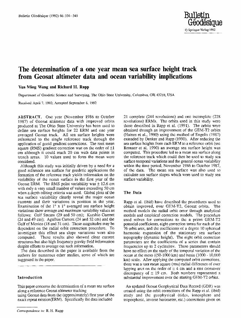
After the gradient corrections were applied, a data record for each point on the reference orbit was made containing the sea surface heights from, up to, 22 ERMs. The total number of such records was 925650. Figure 1 shows the location of every 10th data point. The number of individual sea surface heights at a specific point depends on the availability of the original Geosat data. Table 1 shows the number of data points as a function of the number of sea surface heights (or ERMs) available.

averaging procedure. The two data sets were very comparable with point to point differences on the order of 1 to 2 cm. We then decided to adopt the mean sea surface heights based on the arithmetic averaging since we felt that the iterative re-weighting average could inappropriately down weight sea surface heights in regions of high sea surface variability.

Table 1. Number of Points on Reference Track as a Function of Number of Sea Surface Heights Used to Form Average

No. of SSHs used t0 f°rml averages

2 3 4 5 6 7 8 9 10 11

No. of points % No. of S SHs on reference track used to form averages

17819 119 12 14559 1.6 13 13912 1.5 14 13437 1.5 15 15366 1.7 16 14590 1.6 17 11900 1.3 18 12224 1.3 19 13418 1.4 20 14575 1.6 21 16719 1.8 22

From Table 1 we see that data points for which 12 or fewer sea surface heights is typically 1 to 2% of the total number of data points. Data points computed from 21 and 22 sea surface heights (ERMs) constitute 43% of the total data set.

We next considered two procedures for the computation of a mean sea surface height from the individual sea surface heights. One procedure considered was an iterative averaging/re-weighting procedure described by von Gysen et al. (1991). In this procedure an arithmetic average of the sea surface heights was computed at each point on the reference track. A weighted average was computed where the weights were related to the absolute value of the individual sea surface height residual with respect to the average value. The second procedure was simply the computation of the arithmetic average.

The standard deviation of the mean sea surface at each data point was computed using the arithmetic mean value and the individual values. 99.9% of the values had standard deviations less than + 1 m while 149 values had standard deviations greater than 1.5 m. The standard deviation can be associated with several factors including time variations of the sea surface, residual time dependent radial orbit error, tide model errors, atmospheric correction errors, etc. For the purpose of further discussion we assumed that the dominant cause of the standard deviation was sea surface variability although tidal errors may play a significant role. Since such variability is not expected to be greater than 1.5 m, revised mean sea surface heights were computed deleting the individual sea surface heights that exceeded the original average by the 1.5 m in absolute value.

A set of mean sea surface heights was now available from the iterative re-weighting procedures and the arithmetic

No. of points on reference track

18346 23180 28945 32324 36344 37361 46969 60724 87535 134352 261040

%

2.0 2.5 3.1 3.5 3.9 4.0 5.1 6.6 9.5 14.5 28.2

The mean sea surface along the Geosat track, after correction for the OSU91 sea surface topography model, was compared to the geoid undulations computed from the OSU91A potential coefficient model that is complete to degree 360 (Rapp et al., 1991). The comparison was made for all the mean sea surface heights, and for a case when the mean sea surface heights were based on at least 10 sea surface heights with no residual greater than 1.5 m. The results are given in Table 2.

The standard deviation reflected in Table 2 shows high frequency effects not represented in the potential coefficient model, orbit error, etc. The differences are well within the estimated accuracy (+ 57 cm) of the OSU91A model (Rapp et al., 1991, p. 64). The number of large residuals is significantly smaller when the more reliable (10 or more values) altimeter implied undulation is used in the comparison. The positive extreme difference occurs in an area (Kuril Trench) of high frequency gravity signature and reflects, primarily, information missing above degree 360. The negative extreme occurs in a shallow area just north of South America and may be associated with altimeter tide correction errors.

Sea Surface Height Time Variability

After applying the gradient corrections, estimates of the sea surface heights were available for up to 22 values (from 22 ERMs) at 925650 reference track points. As noted from Table 1 28.2% of these points had a complete sequence of 22 values spanning the time period from November 1986 to November 1987 with a sampling interval of 17.05 days. The remaining points had less than 22 values due to incomplete observation or rejected data in a ERM data set. The data on the reference track enables us to study the variability and the temporal changes in the ocean surface.

CO

CO

0 F'- OJ

CD

f~

LO

Z

-J 0 CO

LFJ

0 CO

o

o 00

o o)

o

c3 03

o

o co

cD

~OOlIIUq

o

0

CD CO

[

C~

0 f_O

I

0

I

CD

I

C2)

C~

CO c~ o'3

o o

o r ~

o

o

oJ bJ £3

b -

o z

(:3 . - I CO

o LO

g

N

0 ~0

0 0'3

C23 0

I

0

0

0

0

0 ,:I.1,

© £

0 z.,

©

339

340

Table 2. Comparison of the Difference (Geosat--OSU91A) Between the Corrected Mean Sea Surface and the Geoid Undulation From OSU91A on the Reference Geosat Track

Number Mean Diff. Std. Dev. RMS Min Diff. Max. Diff. Num. of IDiffl >_ lm Num. of IDiffl > 2m

All Data Selected Data* 925650 -2 cm 38 cm 38 cm -6.5 m 6.4 m 28656 3962

798270 0 cm

29 cm 29 cm -3.3 m 4.5 m 12762 844

* Mean Sea Surface from at least 10 sea surface height values.

The sea surface variation at point i of the k th repeat track is defined as follows:

SSH(Vik) = S S H ~ - S S H i (2)

where S S H i is the mean sea surface height at point i on the reference track. Statistical information on the behavior of the sea surface variation when at least 10 ERM values (with no residual greater than 1.5 m) were available to form the mean sea surface is given in Table 3. The RMS value is computed for each possible point on the reference track with two computations made depending on the depth near the point.

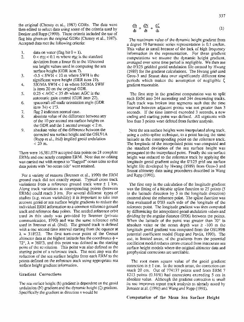
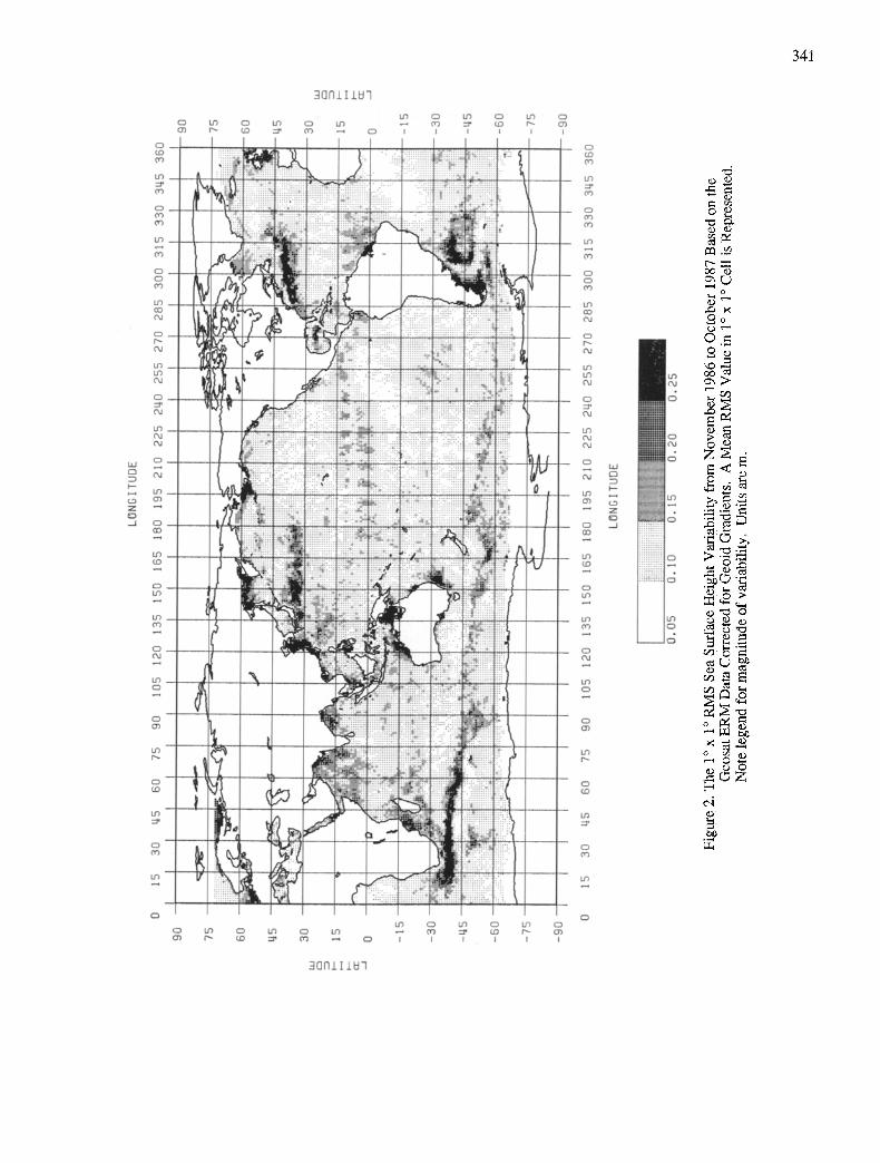
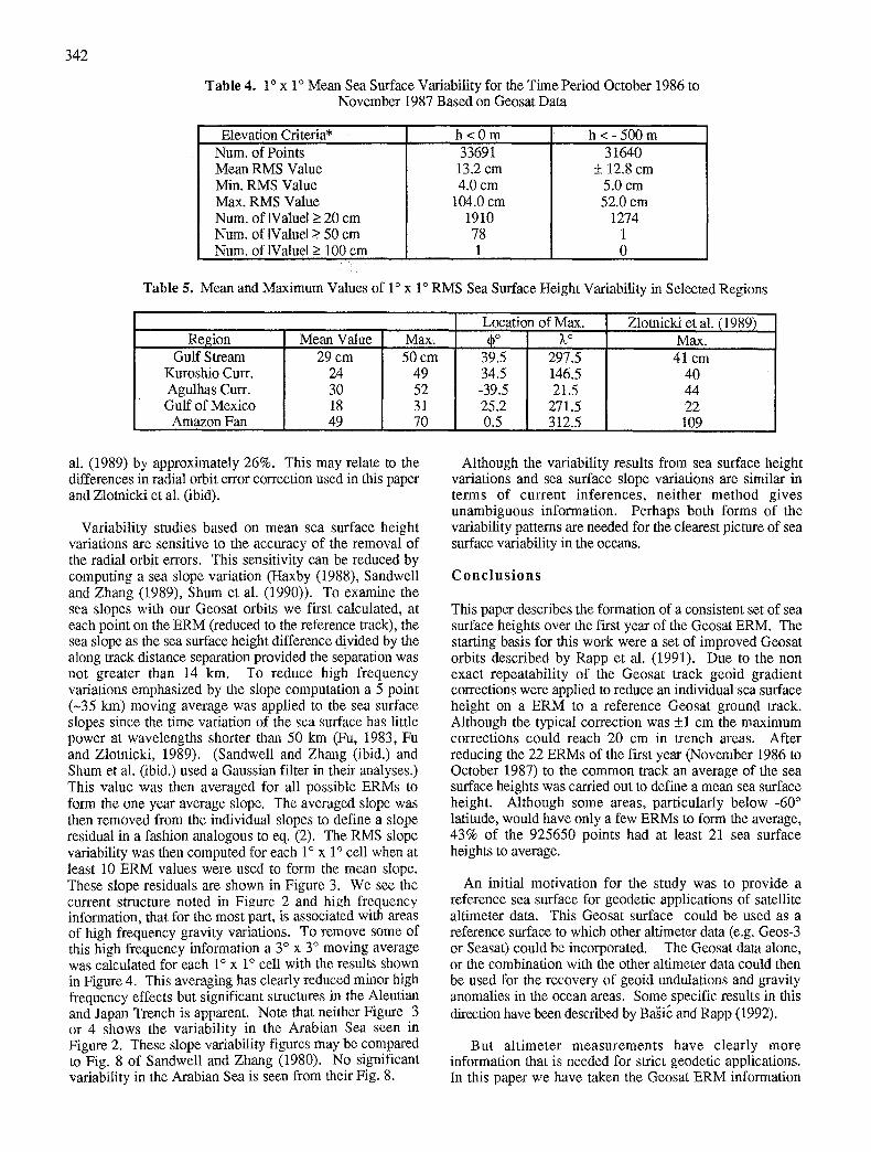
Statistical information on this variability is given in Table 4. The highest variability occurs in the areas such as the Agulhas, Falkland and Kuroshio Current, and the Gulf Slxeam, etc. These results are generally in good argument with the results of Zlotnicki et al., (1989) who analyzed just 3 months (November 1986 to January 1987) of Geosat data, and to Sandwell and Zhang (1989, Figure 8) who used one year of Geosat data. The apparent variability signatures of the North Equatorial Current and the North Equatorial Countercurrent is seen in the Pacific Ocean as a double band. As noted by Zlotnicki et al. (ibid) the signatures seen are dependent on the orbit error removal process. However, Zlotnicki (1992, private communication) has pointed out that much of the variability signal seen in this

Table 3. Statistical Information on Sea Surface Variability in the Time Period October 1986 to November 1987 When at Least 2 Values are Used to Form the Mean Sea Surface Height

Elevation Criteria* h < 0 m h < - 500 m Num. of Points Mean RMS Value Min. RMS Value Max. RMS Value Num. of Igaluel ___ 20 cm Num. of IValuel _> 50 cm Num, of IValuel >_ 100 cm

798270 12.9 cm 2.8 cm

107.6 cm 51770 1256

6

763509 + 12.6 cm

2.8 cm 61.9 cm 40576

187 0

* a data point is not used if the elevation criteria is not met.

From Table 3 we see the significant reduction in large variability estimates when the -500 m deletion criteria is applied. For all the ocean points comparisons 0.157% have an RMS variability > 50 cm. This percentage is reduced to 0.024% when the shallow (h > -500 m) water

• criteria is used. In the shallow water case 94% of the values have a variability < 20 cm. The reason for the large variability in shallow areas is probably due to inaccurate tide models in these areas.

In the next step the mean RMS variability within a 1 ° x 1 ° cell was computed using the residuals defined by eq. (2) when at least 10 values were available to calculate the mean value. A plot of the sea surface height variability as implied by the variations in the 1 ° x 1 ° cells is shown in Figure 2.

equatorial region is caused by M2 tidal errors in the t ide correction provided on the Geosat GDR. The role of improved M2 tides in the estimation of sea surface heights is described by Jacobs, Born, and Parke (1991).

Plots of the 1 ° x 1 ° RMS variability values were made in several different areas. In most areas of significant current structure it was not difficult to identify such structure through the contrast between the higher variability in the current and the lesser variability outside the current. With these plots we calculated the mean variability for five areas and selected the 1 ° x 1 ° cell with the largest variability. These results are shown in Table 5.

From the table we see that the maximum variability is approximately 80% greater than the mean value. The large variability in the Amazon Fan represents, most probably, tidal errors in the relatively shallow area. Our maximum values exceed the maximum values noted by Zlotnicki et

L~

F-

Z

:=.x_. .:..:::..

.-:;:...;::..

0

kO r22) 12; (23 kr; Lr) Gz) L~ C) LD

CO ~ CO J i I I I

r - -

i -

1

I

ko ~ I.o (221 I ~

1 I I 1 I

~HNIIIU']

::::::::::

:::::~:;:

r -

g--

7-

O LP C:~ 1~ I ~ ~O ~ ~ ~ O

O~ I

C) (D

[D ::P CO

LO

O'3

CD CD OD

@ Od

C2~ r~ f~d

kD

ff,j

(23

~d

kO C'd ~d

(23

k~

(Z3 00

qO

C~ gr~

N (zz~ Od

I

C~

k -

/

~-,r)

Oo

0.~

c4

341

30N±I±U3

342

Table 4. 1 ° x 1 ° Mean Sea Surface Variability for the Time Period October 1986 to November 1987 Based on Geosat Data

Table 5. Mean and Maximum Values of 1 ° x 1 ° RMS Sea Surface Height Variability in Selected Regions

al. (1989) by approximately 26%. This may relate to the Although the variability results from sea surface height differences in radial orbit error correction used in this paper variations and sea surface slope variations are similar in and Zlotnickietal. (ibid). terms of current inferences, neither method gives

unambiguous information. Perhaps both forms of the Variability studies based on mean sea surface height variability patterns are needed for the clearest picture of sea

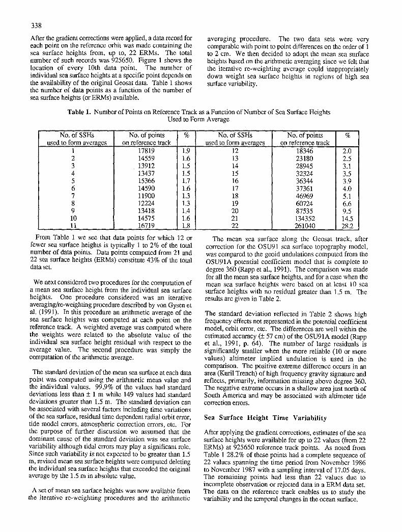
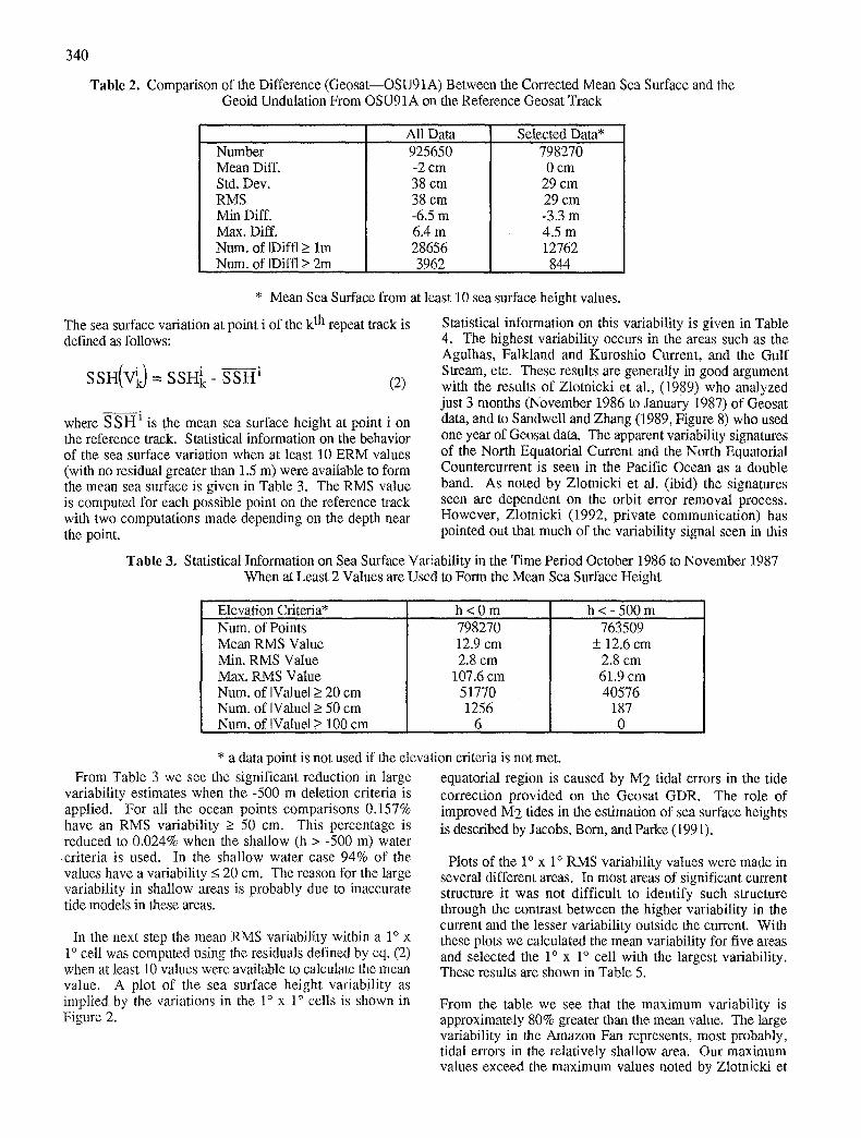
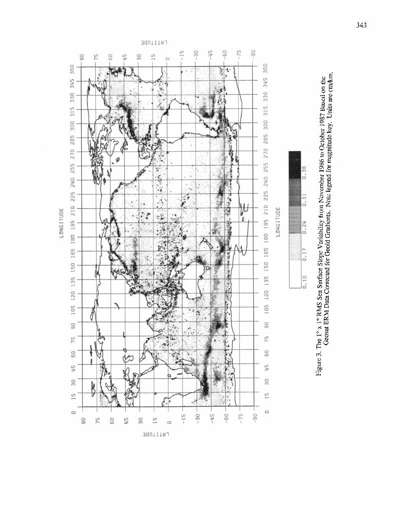
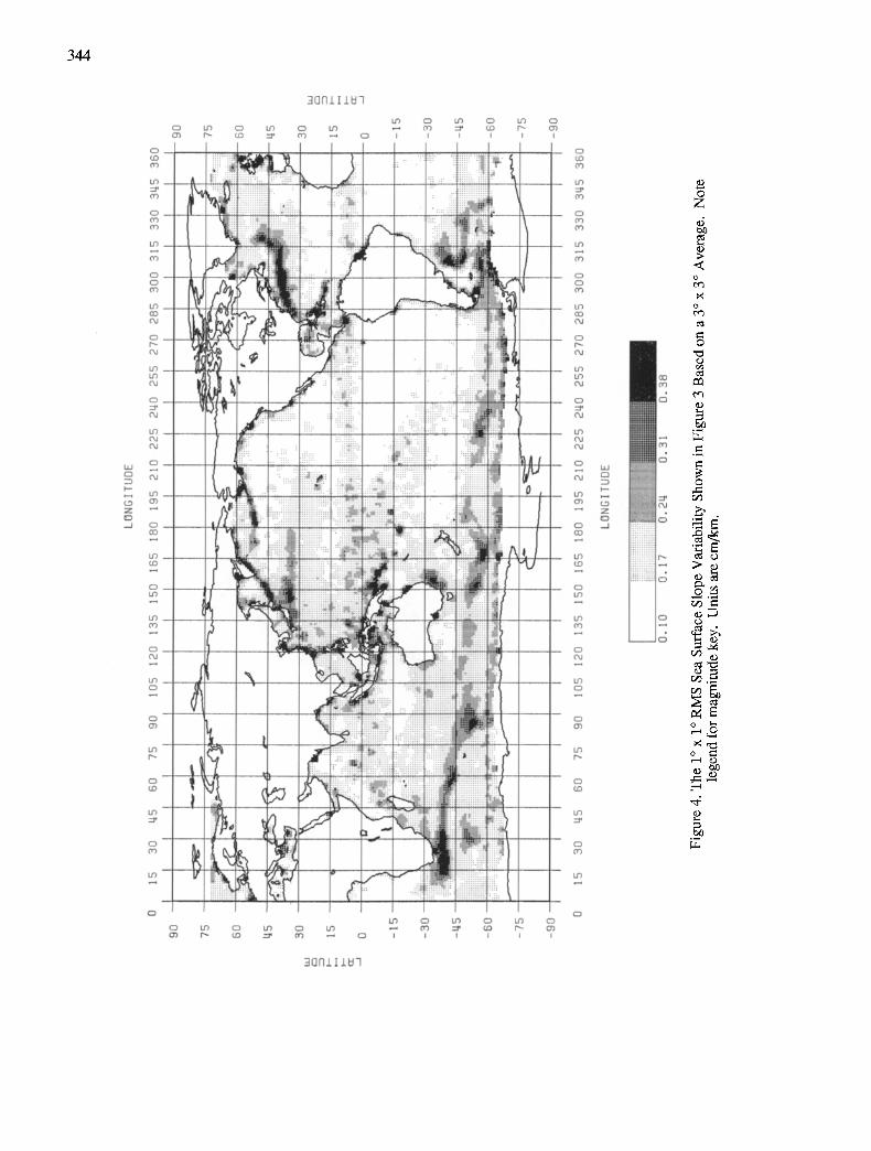
variations are sensitive to the accuracy of the removal of surface variability in the oceans. the radial orbit errors. This sensitivity can be reduced by computing a sea slope variation (Haxby (1988), Sandwell C o n c l u s i o n s and Zhang (1989), Shum et al. (1990)). To examine the sea slopes with our Geosat orbits we first calculated, at This paper describes the formation of a consistent set of sea each point on the ERM (reduced to the reference lrack), the surface heights over the first year of the Geosat ERM. The sea slope as the sea surface height difference divided by the starting basis for this work were a set of improved Geosat along track distance separation provided the separation was orbits described by Rapp et al. (1991). Due to the non not greater than 14 km. To reduce high frequency exact repeatability of the Geosat track geoid gradient variations emphasized by the slope computation a 5 point corrections were applied to reduce an individualsea surface (-35 kin) moving average was applied to the sea surface height on a ERM to a reference Geosat ground track. slopes since the time variation of the sea surface has little Although the typical correction was + 1 cm the maximum power at wavelengths shorter than 50 km (Fu, 1983, Fu corrections could reach 20 cm in trench areas. After and Zlotnicki, 1989). (Sandwell and Zhang (ibid.) and reducing the 22 ERMs of the first year (November 1986 to Shum et al. (ibid.) used a Gaussian filter in their analyses.) October 1987) to the common track an average of the sea This value was then averaged for all possible ERMs to surface heights was carried out to define a mean sea surface form the one year average slope. The averaged slope was height. Although some areas, particularly below -60 ° then removed from the individual slopes to define a slope latitude, would have only a few ERMs to form the average, residual in a fashion analogous to eq. (2). The RMS slope 43% of the 925650 points had at least 21 sea surface variability was then computed for each 1 ° x 1 ° cell when at heights to average. least 10 ERM Values were used to form the mean slope. These slope residuals are shown in Figure 3. We see the An initial motivation for the study was to provide a current structure noted in Figure 2 and high frequency reference sea surface for geodetic applications of satellite information, that for the most part, is associated with areas altimeter data. This Geosat surface could be used as a of high frequency gravity variations. To remove some of reference surface to which other altimeter data (e.g. Geos-3 this high frequency information a 3 ° x 3 ° moving average or Seasat) could be incorporated. The Geosat data alone, was calculated for each 1 ° x 1 ° cell with the results shown or the combination with the other altimeter data could then in Figure 4. This averaging has clearly reduced minor high be used for the recovery of geoid undulations and gravity frequency effects but significant structures in the Aleutian anomalies in the ocean areas. Some specific results in this and Japan Trench is apparent. Note that neither Figure 3 direction have been described by BaSic and Rapp (1992). or 4 shows the variability in the Arabian Sea seen in Figure 2. These slope variability figures may be compared But altimeter measurements have clearly more to Fig. 8 of Sandwell and Zhang (1980). No significant information that is needed for strict geodetic applications. variability in the Arabian Sea is seen from their Fig. 8. In this paper we have taken the Geosat ERM information

343

O LO E:] LO O LO 09 r ,~ Co :::9 o~

cD o . . . . . . . . . . . 2 o L : -~ , I IGJ : " ' "

oo :f~'L-"'iLii: Ff . . !~:i]" ! . , : ! : " - " . ~T :

C~

CM

CD C'~

I - - ~ kO _ _

C9 C~ Z

-J ~ : 3 _ _ CO

LO CO

O LO

LO ( O

OJ

LO O

CD

kc) r ~

O ( O

k ~

O t ~

k ~

O

r _ . - " :~. #: ! : . :

~,~Gi~!i...¢- ." ., ':~'#'''~':"

I ! L . : : " .. . . . : " : ' : " . . . . . " ,,a,t.:,, ....: :,~:~:~

: • '~::',:,~~,~i~i~.1 " ' '" `~j:~': ~ i . ~. :~: : ' 7 ! !i i!) i~::: :: : : : ~ :

! ! i . i i ~ I: ...:~iii!iiiil!:iii~!:ii!i:i :~,:{;:~i ::: ':: ' ..::::"=':~:'h':!:=.::! : ,...l,i;!~i"!i~

~i:~:~.:' ..~i.)~i )~;].i::~ii:~;i'" . . . . . . :i:.:i~yi)ii!t:;ii):T!~ :~:: ~",~;~:"

.. =:ili,ii~i,:; iiL~i~:#: i:: : . . . . . . . . .

. " " )~ ~i, :~;~:~:~:: d:~.i~;Ti.:.,"~

N ' : n~ :~ri,~,;i[i~.i:~ :!

I ~ i i ~ ' i i i

,

I

O ~ C2~ k ~ (23 127

I f ) O LO

C3 1 i I

' , : ? : , :iiiiiiiiiii ". ! i : -:1 .......... . . . . . . iiiii~ . . : . . : . : : :::

o r - . : . " '!i~i:~! ~ ! ~ i ~ i~::i~ ~ ~ ,

=: = ..-:.

• ? : : :iii',i

..i:.- ':' .. :::- . i i i i i i l " < : : ! : [ : : i i : :"~iii~!!i

" " .= L:i]i~12~ • .. ,,. ;17 Y # : : : ! i ;=:~::ii~ili

" " : . - ~*:-:!i~!~ i " : : : " : : : : : i~, ; i )

• .i °: '~:~.'.::!:::: . . . . . .: . . . . . . . . . :d:!!i; if! i

. . . . . . . . . . o . / L - - : ~ ' . . " : . : ~ t [ ! !

~.::ii~::i :: ........ i~ ~::.::ti!ai

....... _~: ::TP :;: .... +::::,, +i:,'rL~iiiiii~i

................... :,, iiii!!iiiii~ ',~::~!:.~,~ , .i:: I .-..":L~!~:~' t'..'l!i~i!!~ ~ . ~ " . . " . : i:i: :~i,:~,~:.~

:.,.::::~..~i;!!: !iiii:)i::ii ~i-~

:: ~ii ~,'o,, iii!~it . . . . . . . .

: $ iiiii :; • , ~ .

I LO

I

c o ~ I

]!ii!),,,

~ii::l

i@.::~

,i~. n

~N

: 0

t )

O~

o

CO

LO

CO

O

o~

LO

G ]

C ] C:] CO

__ LO CO OJ

O F ~- Od

LO

C?

Od

Od Od

~ N H -

CO

kD CO

k ~ CO

O

kO

O O~

LO r ~

LO

I

O3

If)

CZ) CZ~ LF) E3 bO

I I I I I

~m

oo

o

o

o

~8

~d

~OOLIIU]

3 4 4

E3

0

C3 ! . O3 CO

O3

CO

C'd

g ; Od

co . ! U3 O,J

(;3 ::::P Ckl

CO C'd Od

ta.J C:?

C~ C~

N CD

_ J C3 _ _ CO .---t

LD c o

C3 c o

kO _ _ O'3

C3 OJ

kD C3

(23 ~3

CO

c o

k ~

O

ts3

SOOlIIU]

co :;;P c0 .-.-, co : ~

o i t

. . . . . :::::::.:: ::...:::

:::: :::~:::: ::::::+..: i!!::~::iii:?p,

!'+i++!!,!i .........

+ . . . . . .

: : : : : . . . . . . . .

: ~:: ~i ~i7: i i +:' -= .. .. ...... "++++ ::i+::::::+!+

t ~ " ::-::;++ ...........

, , , ++++}|,+i++++;+++++ ++++++++++::

.+,, iii+, ....... +++++++++

.... ::::::::.

. . . . . . . . . ~:::~ !i!!!!!!! ~ l r~ :~! . l .:.::.!i!! !!!!!::i::i::

::::::~::. ~ ........... ~++++++:++

r'iii!iiii:~i

] i i i : ~ i

. - . _ ,,.~ll~++!.ff+ +

+

: m::r

m I,I

++i++++++~ ++3~ I'm;;,~

:+++ii+i+++ +.:+++++i

~ii+ii. :::::::

:+i+~+

:+12ili:;;!ii ~ti!![ :2.2222"

:~iiiii:: ii!+t::

""~'!:f!F"

:::::::. .... ::::: ::::.::::. :+++}++~+

"i++i++i

+++!+++iii ~siiiN}?+~

++++#++ 1112.!?!

N N ~:;i?iiiiii ::.:::++tt+¢ :++U+~'+'+

.;.::::::.++

i ; i i i i i i i i

::!iiiii+ Nii!~i ~i:::ii!ili

::~IN i .:::::::~

+m:.::

t+++- ~

• :ii,~ iiiiiiiiiiiiii : :: ::::;:::::::::

:: i i i i i~ ::y-= • . . . . . :~ ~ + ~

~::.iiil;i ~i?i;;i~ii ~ + ' + '+++++++++ +~;++++~+i p ~+++~ +~+;+++++,+ +++++t

~i+:++++++'+'++++++ |++++++ +.+++i+++++I

.-- !::~+~!!~++ +/ :...::::::

~iili

• :" :iili!

: .., .: v ::::~

• :::::::.

::h+~L':+~ . . . . .. ++++~+t - $iiiif!:..:i ~i~ !

, ,+: !lii~i!iiiiii:~+ :: ! iN

i!ii;;~Fii : ! : : ¢ i i • : ;i!+ii+iiiii!ii ++i~+i++i+! ;i;ii+;;+:~+ ;:+ +++ ~++~+ ++++++++++t +..+++++ ........ +; P+ PP!+++++++ ++++~++++: +~::+ . . . . . . . :+ ~ ++:i+~+:++~++++++ ii!!tiii ++++!+i+ :iit::>; +,':::~

! ! ~ ~ii!i; i!! i, iiiiii,!!iil

+ .,

. . . . + <~:+,. P+++++++++++++

: ++i

NI + ~ +?:+i++++i +-+iiiii+i +++++++i + +~++++++++++ +++++++++++~

~++i+;;: +++++i+#+ +.++++++++++ i+#++~+J+i .Ji+ ::+++++++q+ +iNIII+N+++ iiiii+::. +:+ :i+ii i!iiiiiiiiii Nig!iii iiiii;..+i! .+iiiiii !!iiiiiiiiii ' ~

~i{!{iiF Y!{i!iiii!! i++iii++ii++ +!!!!+!!¢~+I +++++: ++++::++++++ :+++~++++oo+ +++++++++++' +ii!i++++++ :+++:+++++++ . . . . . . . : ......

:++++i+++~ ~ i + :C+%+ ++ ++-++ ++++++++++I

. : " ~ ++++~i+++ ++++I+

i ....... +:~ ++++++. :++t

,"-" .... i+'. +o-+++ +++++%++~+ "+++I ++++~+++++ ............ i¢+++++++i+

P

LO p-.

I

C~ LO o I.~ o LO

N¢I , lJ

:::;~:

i!iiiii]+

ii~#P..P, 1

f i i i f

i i i@

!!!!¢

~i++i

~+ iIP" ml

L ' !

+iii ,

iii' '

-4--'--- J

!!~: 3 t++ t'

N

Ji++l| +i+'J

~3 lil~ |

N iiilt

CD ( O qO

CO

0 CO CO

LO

CO

_ _ CD 0 CO

LO O3 Od

_ _ CD p-,.

Od

_ _ LO Lf) OJ

CD z ~ C~

LO 0 4 O+J

CD

C~J C3

B-+ LO C~ CO "+++ Z

~D 0 _-I

c ~ k o

u 3 c o

c o Od

LO CD

I <23 0 3

kf3

f2? CO

kD =:P

C?) U3

kD

I,D (2:3 Lf~ (Z3 kl~ C3 ~ ~ ¢ . D r ~ Or1

t I I I L 1

¢ o

i> < o

o

0

t~O

0

.

~ ' ~

O

' 2

- 4

3 ~ n i l l U ~

with our improved orbits to study the time variability of the ocean surface. This has been done by computing the sea surface height variations and sea surface slope variations within the full one year in which the Geosat data available. Figure 2, 3, and 4 clearly show the major current structure from the variability estimates. Color plots of the variability have also been produced which carry additional information. One notes from Table 3 and 4 that the RMS variability averages + 13 cm with only 187 (out of 763509) values exceed 50 cm. The removal of shallow water (h > -500 m) data points reduced the number of larger residuals substantially. These points are most probably unreliable due to tidal errors in the reduction of the altimeter measurement.

Much work remains to be done with the altimeter data set. !n the oceanographic area one can study the sea surface variation on a monthly or seasonal time scale. One could use the dam for comparison with tide gauge variations especially in deeper water areas where the influence of erroneous tides will not be as great as in coastal regions.

A tape with all 22 ERM data and the averaged sea surface heights is available from the authors. Acknowledgement

The research described in this paper was supported through NASA's TOPEX Altimeter Research in Ocean Circulation Mission funded through the Jet Propulsion Laboratory under contract 958121.

R e f e r e n c e s

BaSic T RH Rapp (1992) Oceanwide prediction of gravity anomalies and sea surface heights using Geos-3, Seasat, and Geosat altimeter data, and ETOPO5U bathymetric data, Rep. No. 416, Dept. of Geod. Sci. and Surv. Ohio State Univ., Columbus

Brenner AC CJ Koblinsky BC Beckley (1990) A preliminary estimation of geoid induced variations on repeat orbit satellite altimeter observations, J. Geophys. Res., Vol. 95, No. 13

345

Fu LL V Zlotnicki (1989) Observing oceanic mesoscale eddies from Geosat altimetry: Preliminary results, Geophys. Res. Ltrs., 16 (5), 457-460

Haines BJ G Born G Rosborough J Marsh and R Williamson (1990) Precise orbit computation for the Geosat exact repeat mission, J. Geophys. Res., 95, C3, 2871-2885

Haxby W (1988) Sea surface slope variability from Geosat, 11/86-9/87, OceanOgraphy, 1, 3, p. 8-9, November

Hwang CW (1991) High precision gravity anomaly and sea surface height estimation from Geos-3/Seasat satellite altimeter data, Report No. 399, Dept. of Geodetic Science and Surveying, The Ohio State University, Columbus

Jacobs G A G Born M Parke (1991) Construction of the global annual cycle from Geosat altimeter data with an estimation of the M2 tidal alias error, (abstract), EOS, Trans. AGU, Supplement, Oct. 29, 1991, p. 258

Rapp RH NK Pavlis (1990) The development and analysis of geopotential coefficient models to spherical harmonic degree 360, J, Geophys. Res., Vol. 95, p. 21,885-21,911

Rapp RH YM Wang NK Pavlis (1991) The Ohio State 1991 geopotential and sea surface topography harmonic coefficient models, Rep. 410, Deptl of Geod. Sci. and Surv., The Ohio State Univ., Columbus

Sandwell D B Zhang (1989) Global mesoscale variability from the Geosat exact repeat mission: Correlation with ocean depths, J. Geophys. Res., 94 (C12), 17971-17984

Shum CK et al. (1990) Variation of global mesoscale eddy energy observed from Geosat, J. Geophys. Res., 95 (C10), 17865-17876

Cheney RE BC Douglas RW Agreen L Miller DL Poorer, NS Doyle (1987) Geosat altimeter geophysical data record user handbook, NOAA Technical Memorandum NOS NGS-46

Wang YM RH Rapp (1991) Geoid gradients tor Geosat and Topex/Poseidon repeat ground tracks, Report No. 408, Dept. of Geodetic Science and Surveying, The Ohio State University, Columbus

Denker H R Rapp (1990) Geodetic and oceanographic results from the analysis of 1 year of Geosat data, J. Geophys. Res., 95, C8, 13,151-13,168

Zlotnicki V L-L Fu W Patzert (1989) Seasonal variability in global sea level observed with Geosat altimetry, J, Geophys. Res., 94, C12, 17,959-18,237

Engelis T (1987) Radial orbit error reduction and sea surface topography determination using satellite altimetry, Rep. No. 377, Dept. of Good. Sci. and Surv. Ohio State Univ., Columbus

Fu LL (1983) On the wave number spectrum of oceanic mesoscale variability observed by the Seasat altimeter, J. Geophys. Res., 88 (C7), 4331-4341.