Download - The damage costs of climate change towards a dynamic representation

ELSEVIER Ecological Economics 19 (1996) 67-90

E C O L O G I C A L E C O N O M I C S

Analysis

The damage costs of climate change towards a dynamic representation

Richard S.J. Tol * Institute for Ent'ironmental Studies, Vrije Universiteit. De Boelelaan 1115. 1081 HV Amsterdam, The Netherlands

Received 19 September 1995: accepted 23 February 1996

Abstract

Economic assessments of climate change impacts are commonly presented as the effect of a climate change associated with a doubling of the atmospheric concentration of carbon dioxide on the current economy. This paper is an attempt to express impact as a function of both climate change and socio-economic change. With regard to climate change, issues discussed are level versus rate of change, speed of adaptation, speed of restoration and value adjustment, and symmetry. With regard to socio-economic change, agriculture, migration and the valuation of intangible losses are addressed. Uncertainty and higher order impacts are treated briefly. It is qualitatively argued and quantitatively illustrated that these issues matter a great deal for the damage profile over the next century. A damage model, based on my best guesses, is presented in the Appendix.

1. Introduction

Estimates of the socio-economic damage costs of cl imate change regularly appear in the literature on the economics of climate change, the most comprehensive and prominent being the assessments of Cline (1992), Fankhauser (1995), Nordhaus (1991, 1994), Titus (1992) and Tol (1995). Working Group 3 of the Second Assessment Report of the Intergovernmental Panel (Pearce et al., 1996) assesses the current knowledge. This paper evaluates the state of the art and attempts to take it a few steps further. Its most practical contribution is the damage costs module presented towards the end of the paper. The module is a first, rough attempt to include some of the dynamics that climate change impacts inhibit. The rest of the paper discusses such dynamics in a more qualitative way.

The starting point is Table 1, which contains estimates of the damage due to a doubling of the atmospheric concentration of carbon dioxide. Cline, Fankhauser, Nordhaus and Titus enumerate the detailed impact studies, compare and review them, cast them in a common metric and then add them up to get a first impression of the overall effect. They have done an admirable job, but it is only the first step, as they themselves hasten to

* Tel.: (31-20) 444-9555; Fax: (31-20) 444-9553; e-mail: richard,[email protected]

0921-8009/96/$15,00 Copyright © 1996 Elsevier Science B.V. All rights reserved. PII S0921-8009(96)00041-9

68 R.S.J. Tol / Ecological Economics 19 (1996) 67-90

Table 1

US cl imate change d a m a g e est imates (2 X C O 2 - 1095 (1990)) a

Loss ca tegory Fankhause r (2.5°C) Cline (2.5°C) Nordhaus (3.0°C) Titus (4.0°C) Tol b (2 .5oc)

Coastal defence 0.2 1.0 7.5 1.5

Dry land loss 2.1 1.5 3.2 c 2.0

Wet land loss 5.6 3.6 - - 5.0 d 5.0

Species loss 7.4 3.5 - - - - 5.0

Agr icu l ture 0.6 15.2 1.0 1.0 10.0

Forestry 1.0 2.9 - - 38.0 - -

Energy 6.9 9.0 - - 7.1 - -

Wate r 13.7 6.1 - - 9.9 - -

Other sectors - - 1.5 38.1 e __ __

Ameni ty . . . . 12.0

L i f e / m o r b i d i t y 10.0 > 5.0 - - 8.2 37.7 f

Air pollut ion 6.4 > 3.0 - - 23.7 - -

Wate r pollut ion - - - - - - 28.4 - -

Migrat ion 0.5 0.4 - - - - 1.0 Natural hazards 0.2 0.7 - - - - 0.3

Total U S A 60.2 > 53.5 50.3 121.3 74.0

(% GDP) (1.2) ( > 1.1) (1.0) (2.5) (1.5)

Total wor ld 269.6 220.0 315.7

(% G W P ) (1.4) (1,33) (1.9)

a Table adapted f rom Tol (1995); the f igures are est imates o f the order o f magni tude . b Inc luding Canada .

c Total land loss (dry- and wetlands).

d Total costs o f sea level rise (protect ion plus dry- and wet land loss).

e Inc luding those not assessed,

f Tol values an Amer ican life more than twice as h igh as Fankhause r does.

acknowledge. The figures of Table 1 are estimates of the order of magnitude of the impact of climate change. The assessments are not comprehensive. Table 1 reflects the first generation of climate impact studies. These studies focus on the impact of one particular state of climate change (the benchmark of 2 X CO 2) on present society. These studies do not, or only in a very simple fashion, assess what the damage would be of non-benchmark climate change, nor do the analyses yield insight into the sensitivity to climate change of possible future societies. This paper discusses the unfolding dimensions of the next generation of impact studies, thus drafting parts of the research agenda for the second generation impact studies. The paper interprets the first generation studies in a way that these can be less unrealistically used in integrated assessment models, l As such, the issues treated here are not new; integrated models exist and contain damage functions which do have climate and development as arguments. However, most integrated modellers confine themselves to stating their assumptions, sometimes testing the sensitivity. Here we bring the underlying thoughts into the open for discussion, highlighting the issues by the damage module of one particular integrated climate change assessment model, the Climate Framework on Uncertainty, Negotiation and Distribution (FUND; Tol et al., 1995).

Table 2 displays the regional distribution of the damage costs of climate change. The figures of Table 2 are to a large extent based on extrapolation of the already very uncertain estimates of Table 1. However, the pattern

L The te rm integrated assessment models ( IAMs) is here restricted to mean those IAMs which pe r fo rm cos t -bene f i t analyses. W e y a n t et al. (1996) discuss the state o f the art o f integrated c l imate change assessment .

R.S.J. Tol / Ecological Economics 19 (1996) 67-90 69

Table 2 Climate change damage estimates (2 X CO z -1095 (1988)) a

Regions b 1 2 3 4 5 6 7 8 9 Total

Coastal defence 1.5 1.7 1.8 0.5 0.0 1.0 2.0 0.5 0.5 9.5 Dryland loss 2.0 0.5 4.0 1.3 0.0 0.5 1.0 0.0 0.5 9.8 Wetland loss 5.0 4.0 4.5 1.3 0.0 1.5 1.5 0.5 0.5 18.8 Species loss 5.0 5.0 5.0 2.5 0.0 2.0 1.0 1.0 0.5 22.0 Agriculture 10.0 - 4 . 2 - 6 . 3 - 3 2 . 5 0.7 11.8 21.0 - 3 . 0 17.5 14.5 Amenity 12.0 12.0 12.0 - 1.0 0.1 0.4 1.2 1.0 0.5 38.0 Life/morbidity c 37.7 36.6 36.9 18.8 0.6 11.4 21.6 15.4 9.0 188.0 Migration 1.0 I. I 0.6 0.5 0.0 2.4 4.4 2.6 1.3 13.8 Natural hazards 0.3 0.0 0.8 0.0 0.0 0.1 0.1 0.1 0.3 1.4

Total 74.0 56.5 59.0 - 7.9 1.3 31.0 53.6 18.0 30.3 315.7 (% GDP) (1.5) (1.3) (2.8) ( - 0 . 3 ) (4.1) (4.3) (8.6) (5.2) (8.7) (1.9)

After Tol (1995); the figures are estimates of the order of magnitude. t' (1) USA and Canada; (2) OECD-Europe; (3) Japan, Australia and New Zealand; (4) Central and Eastern Europe and the former Soviet Union; (5) the Middle East; (6) Latin America; (7) South and South East Asia; (8) centrally planned Asia; (9) Africa. ' The value of a human life is assumed to equal $250000 plus 175X the per capita income in the region.

of vulnerability is clear: The poorer regions are more vulnerable to climate change than the richer ones. The reasons for this will be discussed below.

The paper is built up in the following manner. Section 2 starts with a classification of damage dynamics. The rest of the paper is framed in this classification. Section 3 is on the impact of non-benchmark climate change, that is, the impact of climate change before and after doubling of atmospheric carbon dioxide. 2 Section 4 discusses how the vulnerability to climate change may develop. Section 5 provides some numerical illustrations; the model used for this is described in the Appendix. Section 6 continues with two further topics in dynamics: Knowledge and uncertainty, and higher order impact; these two topics are more sketchily treated and need to be further developed in the future. Section 7 concludes.

2. Classification of damage dynamics

The damage costs as presented in Tables 1 and 2 represent what an equilibrium climate change associated with a doubling of atmospheric CO 2 (to occur somewhere in the next century) would have on the present economy, which is also assumed to be in equilibrium. As mentioned in the introduction, this is a necessary first step. Obviously, for the larger share of the future, we will not be confronted with the benchmark climate change of Tables 1 and 2. Equally obviously, the future economy on which climate change will impact is not the same as the present economy, not only in size, but also in composition. These two issues, non-benchmark climate changes and socio-economic vulnerability, are fully developed in the present paper. Two other issues in dynamics, uncertainty and higher order impacts, remain more hazy for the moment.

Non-benchmark climatic change is discussed in Section 3 along three lines: The shape of the damage function; the level or the rate of climatic change as determinant; and the speed of damage restoration and

2 Economic assessments of climate change impacts are commonly indexed on the global mean surface air temperature and benchmarked on 2.5°C or 3.0°C, supposedly the equilibrium reaction to 2 × CO 2. Actually, climate change impact is driven by regional climate change, which is not restricted secular trends in mean temperature. The use of a global index ignores the many different climatic patterns that may be associated with 2 X CO 2 and hides the possible inconsistencies and implausibilities in the climatic assumptions of the economic analysis or the underlying studies.

70 R.S.J. Tol/ Ecological Economics 19 (1996) 67-90

adaptation, and value adjustment. The shape of the damage function first of all determines the damage before and beyond benchmark climate change, and the impact of cooling. Cooling is of interest because it cannot be excluded regionally, particularly not when taking sulphate aerosols into consideration. In addition, global cooling cannot be excluded in a full uncertainty analysis (Morgan and Keith, 1995). The lack of observations of climate change damage and the limited nature of the physical impact studies force us to use expert knowledge to assess this shape (e.g., Nordhaus, 1994). The Appendix presents my best guess damage functions for the damage categories of Table 1.

A distinction is made between damage due to the level of climatic change and damage due the rate of change. The damage profile over time differs drastically depending on whether level or rate is used. Damage in the rate rather than the level of change would be easier to detect as it occurs earlier. For a number of decades of the 20th century, the rate of climate change was close to the rate projected for the next century; hence, empirical studies could be used to substantiate the damage estimates. Of course, the impact of climate may depend on a combination of level and rate of change, and on past stress.

Damage restoration is important for its obvious capacity to remove loss. A climate shock leads to recurrent damage declining to nought. Damage restoration differs from adaptation in that the former regards the removal of damage done (e.g., reconstruction, replacement), while the latter regards the adjustments to reduce damage from recurrent stress. Adaptation is the adjustment of habits, practices, infrastructure and capital to mitigate the consequences of a phenomenon that happens over and over again. Hence, adaptation to climate change requires that the change is recognised or, preferably, forecasted. Value adjustment is a mix between restoration and adaptation, but it concerns human valuation and preferences rather than physical impacts; it is the process in which people start appreciating the current situation and bury their nostalgic feelings, e.g., for past landscapes

3 and ecosystems. Adaptation and value adjustment are manifestations of socio-economic dynamics. Such dynamics are induced

by climate change. Section 4 discusses the dynamics which are more or less exogenous to climate change. Two issues are discussed: Vulnerability and valuation of intangibles.

A glance at Table 2 shows that the poorer regions are estimated to be more vulnerable to climate change than the richer. This has, inter alia, to do with the greater share of weather-exposed activities, particularly agriculture, in less developed economies. Another reason is the smaller capacity to adapt to and restore damage. This situation will improve with economic development. On the other hand, the increasing pressure of human activity will also influence the exposure of society to climate change.

The next issue is the valuation of the intangible damage. Intangible damage comprises species losses, amenity, life/morbidity and parts of wetland loss, air and water pollution, and migration. Tables 1 and 2 reveal that intangibles constitute a large share of the total damage in the OECD. This is not only because the OECD is less exposed to tangible damage (see the previous paragraph), but also because the rich tend to value intangible losses higher than the poor (relatively to the respective incomes; cf., e.g., Pearce (1980)): intangibles are luxurious goods. Hence, valuation will also change with growth of per capita income.

3. Non-benchmark climatic change

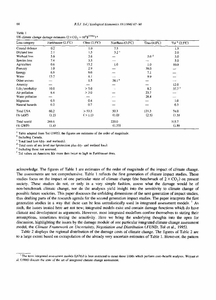
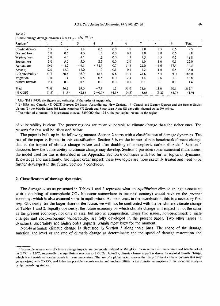
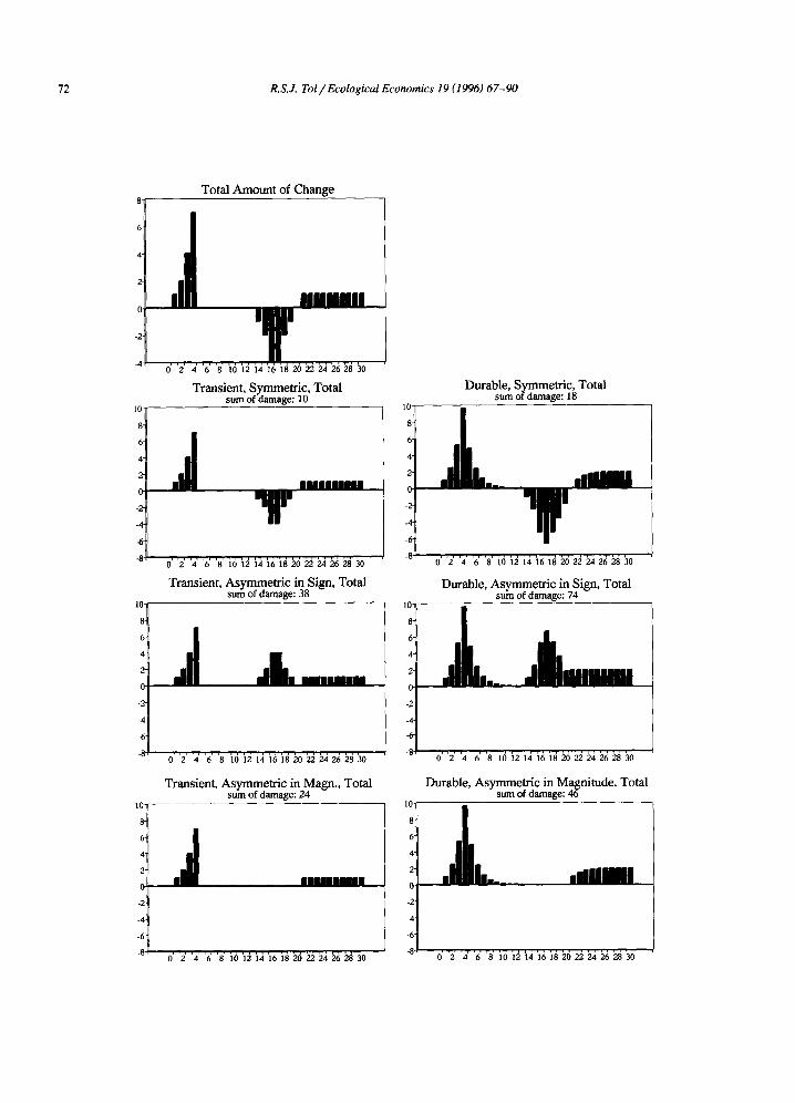
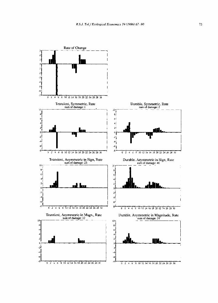
In the previous section we discussed three aspects of the function which describes the damage due to non-benchmark climate change. Here we will take this matter some steps further. Fig. 1 displays 14 graphs to illustrate the importance of a careful design of the damage function. The panels at the top row depict a hypothetical climate change scenario; the level of change is displayed on the left, the rate of change on the right.

3 The bequest/uniqueness/intrinsic value is, of course, lost and will remain so forever; in the long run, this may partly be compensated by such a value of the new situation (cf., also footnote 5).

R.S.J, To l l Ecological Economics 19 (1996) 67-90 71

The scenario is for illustration only; it is not a very plausible future. The panels at the three lower rows represent the damages that correspond to the climate scenario. All damage functions are assumed to be linear in climate change. The second row depicts damages that are symmetric. That is, f ( x ) = - f ( - x ) , or cooling causes equal benefits as a similar warming causes losses. In the third row, damage is caused by the absolute value of change. That is, f ( x ) = f ( - x ) , or cooling and warming result in equal losses. In the fourth row, damage is zero if the change is negative. That is, f(x) = 0 for x < 0, or cooling does not result in damage. Fig. 1 has four columns. The two rightmost columns are for the level of change, the leftmost columns for the rate of change. In the odd columns, damage is instantaneously restored; the systems under stress adapt infinitely fast; or human values are memoryless. In the even columns, the restoration; adaptation; or memory parameter is set to 0.5. That is, 50% of the total damage in year t is experienced in year t + 1 as well, in addition to the damage caused in year t + 1.

Fig. 1 clearly illustrates the importance of the damage specification: Not only are the damage profiles very different, total damage (reported in the subtitles) varies by a factor of seventy. Restoration (adaptation, memory) raises damages considerably. Asymmetries in sign and magnitude also raise costs, the latter by eliminating the benefits, the former by changing benefits into costs. The sum of the damages due to the level of change is higher than the sum of the damages due to the rate of change. This has to do with the smoothness of the scenario: In year 5 the damage due to the rate of change is clearly much higher than the damage due to the level of change. A more erratic scenario would push up the damages due to the rate of change.

Having classified the issues and having demonstrated their potential importance, it is now time to place the damages of Table 1 in the appropriate category.

Damage due to the level of change assumes an optimal state of the climate, at least, in the short term. Any (further) deviation of this (perceived or real) optimum incurs a loss. 4 Also, damage in the level of change neglects induced technological or organisational improvements. Damage due to the level of change implies that, should climate restabilise, damage will be incurred forever. 5 Expenditures on defensive capital (sunk capital and maintenance) are part of the damage due to the level of climate change. The opportunity costs of climate are another part. One example of damage in the level of climate change is change in the agriculture potential; some climates are simply better than others when it comes to growing crops, so there yields will be higher or costs of growing lower (Rosenzweig and Parry, 1994). A second example is human comfort, morbidity and mortality; although one gets used to heat or cold in a way and (medical) technology can do a lot, the human body is better fit for one climate than for the other (Sztrepek and Smith, 1995). The last example is sea level rise. Dryland and wetland loss constitute a clear opportunity cost. Although alternatives will be sought and probably found, the number of options available has decreased so the solution is likely to be inferior. Dryland loss can be prevented by coastal protection; the maintenance and depreciation of the raised structures constitute damages in the level of change (Yohe et al., 1995).

Damages due to the rate of change are transition costs. Adaptation is needed because the expected or accustomed state of the climate deviates from the actual state; adaptation takes time if the information on the future is imperfect or the system is inert. An obvious example is agriculture. If climate changes, a farmer first

4 Any movement towards the optimum would, of course, result in a benefit. 5 Note that one of the major problems with long-lived damage is that higher order effects are likely to outweigh the initial impact. An

illustration of this effect is the flooding of the Channel and the Bering Strait at the end of the last ice age. Although the current situation definitely hampers transport and travel, and myriads of uses could have been found for the land lost, history would have been so much different that it is hard to say whether the inundation was for the better or the worse (unless. of course, one is British).

Fig. 1. The damage costs of climate change for twelve different hypothetical specifications of the cost function for one single, hypothetical climate change scenario. Costs are linear in the total amount (left panel) or rate (right panel) of change. Damage can be transient (odd columns) or durable (even columns); in the durable case, 50% of the damage induced in year t is felt in year t + 1. Damages can be symmetric (2nd row) or asymmetric in sign (3rd row) or magnitude (4th row); asymmetry in sign is represent by taking damage to depend on the absolute value of change; asymmetry in magnitude is represented by assuming no damage for temperature decreases. The figure above the damage graphs is the (undiscounted) sum of the yearly damages. Figure on pages 72 and 73.


Total Amount of Change

ml lnunnnnnn Ik

0 2 4 6 8 10 12 14 16 18 20 22 24 26 28 30

Transient, Symmetric, Total sum of damage: 10

0 2 4 6 8 1 0 1 2 1 4 1 6 1 8 2 0 2 2 2 4 2 6 2 8 3 0

Transient, Asymmetric in Sign, Total sum of damage: 38

0 2 4 6 8 1 0 1 2 1 4 1 6 1 8 2 0 2 2 2 4 2 6 2 8 3 0

Transient, Asymmetric in Magn., Total sum of damage: 24

Durable, Symmetric, Total sum of damage: 18

.I [k.. dnlill

0 2 4 6 8 10 12 14 16 18 20 22 2426 28 30

Durable, Asymmetric in Sign, Total sum of damage: 74

I ]

0 2 4 6 8 10 12 14 16 18 20 22 24 26 28 30

Durable, Asymmetric in Magnitude, Total sum of damage: 46

,I L .,,..

0" 2 "4 6" 8 10 ]2 i4 16 18 2 0 2 2 2 4 26 28 30 0 2 4 6 8 10 12 14 16 18 20 22 2426 28 30


2-

1-

0

-1

-2"

-3-

-4.

-5-

-6

Rate of Change

hll n]

Transient, Symmetric, Rate Durable, Symmetric, Rate sum of damage: 1 sum of damage: 2

4 .Jir o • I , , , , , d i d , . . . I I v - • I

-2

-4

-6

-8 0' '2' '4' '6' '8' i6 i2 izi '16 il~ ")6 22 2.4 26 213 30 ' 81' 0' '2' '4' '6' 'S' i6 ]} i4 '16 '10 20 ~. 24 ')6 ")13 30

10

Transient, Asymmetric in Sign, Rate Durable, Asymmetric in Sign, Rate sum of damage: 23 sum of damage: 46

"

0 2 4 6 8 10 12 14 16 18 20 22 24 26 28 30 0 2 4 6 8 10 12 14 16 18 20 22 24 26 28 30

10"

8

6"

4"

2

0

-2

-4

-6

-8

Transient, Asymmetric in Magn., Rate sum of damage: 12

,,ll h,,

Durable, Asymmetric in Magnitude, Rate sum of damage: 24

0 2 4 6 8 10 12 14 16 18 20 22 24 26 28 30


has to recognise that the unusual weather should be considered a change, not a fluctuation. Then, she has to redesign her practices (assuming that she was previously at optimum). The same goes for any system that is tuned to the present climate. Successful adaptation can take away quite a substantial part of the damage. For instance, Rosenzweig and Parry (1994) estimate a cereal yield decrease of 1-8% worldwide without adaptation, but a decline of 5% to a 35% increase with 'full ' adaptation. Kalkstein's figures for heat-stress-induced mortality without acclimatization are six times higher than the figures with acclimatization (Kalkstein, 1989, 1993). 6

Restoration refers to damage done; if restoration is not possible, the impact is irreversible. Damages that take time to restore are, for instance, property lost in a storm or flood, or damage to crops and trees. Emigrated or deceased people are not necessarily economically replaced at a short notice. It would also take some time before alternatives are found for the economic use of land lost due to large-scale inundation.

In the long run, value adjustment is probably more important than damage restoration. It occurs when the climate (or the system that is valuable) deviates from the reference state. Over time, the memory of the reference fades, and the new climate becomes better appreciated. Examples include the amenity value of climate and the value attached to landscape and ecosystems.

Symmetric losses are equal in order of magnitude if climate changes in one direction or the other, and have the same sign as the change. An example, at least in sign, is heat stress, leading to more casualties if it gets warmer and less if it gets colder. Asymmetry in magnitude implies that the loss due to a change in one direction is greater than the loss suffered from the same change in another direction. This is the case if the combination of costs and opportunities is highly non-linear in climate (for instance, tropical cyclones) and in case the change affects finite stocks (for instance, wetland and species loss); in addition, the change has to be non-marginal. Asymmetry in sign implies that changes in any direction incur a loss. An example is deviation of reality from the expectation, which in one direction causes damage and in the other forgone profits. An example is tourism which can have overcapacity or undercapacity if the weather deviates from the expected. Some damages are both asymmetric in sign and in magnitude. Sea level rise is an example. Sea level fall is likely to be much cheaper than sea level rise. In case of sea level fall, only harbours and canals have to be refitted; whereas in case of a rise the whole coastline needs to be readjusted. Land loss is another example of asymmetric damage; as land is scarce, the opportunities gained by X additional square kilometres are worth less than the opportunities lost by X square kilometres lost.

Other studies have also addressed the matter of non-benchmark climate change damage. Hoel and Ivaksen (1993) use a representation in which the damage is partially induced by the rate and the level of change, depending on one additional parameter. I prefer two separate damage functions for clarity. The main difference is, however, that here damage categories are treated individually. Damage functions with different dynamic properties can often not be comprised to one function encompassing the different dynamics. The structure proposed here and the structure of Hoel and Ivaksen (1993) are not additive over various damage categories. Peck and Teisberg (1994) discuss the implications of (aggregate) damages due to the rate and total climate change on optimal emission abatement in the context of their model CETA, without expressing a preference. Again, damages are lumped together in one single damage function. That is, D, = ~tT, ~, with D damage, t time and T the global mean temperature in deviation from the reference level (usually, pre-industrial or 1990). Alternative, D, = ct ATt~, with AT t the change in temperature (usually, per decade). Peck and Teisberg (1994) conclude that the exponent of the damage function is more important than whether the rate or level of change is used. Damages in the rate of change occur more upfront and are more sensitive to the benchmark change chosen. The PAGE model (Hope et al., 1993) has damage functions in the level and the rate of change, and uses different functions for different damage categories. The damages in ICAM (Dowlatabadi and Morgan, 1993)

6 Note that the assessments of Table 1 and Table 2 assume full acclimatization; even then, life loss accounts for 1/15 to over 1/2 of total damage.


also depend partly on the rate of change and are separated with respect to the damage category. The DICE (Nordhaus, 1994) and MERGE (Manne et al., 1995) models specify damage in terms of the level of change. The damage modules of 1CAM and CETA are the only ones that allow for damages which last longer than the period in which they were caused. None of the damage modules explicitly addresses symmetry.

The shape of the damage function varies from linear to cubic (i.e., [3 is between 1 and 3) in the models discussed in the previous paragraph. The choice is ad hoc. For damages in the level of change, the linear specification leads to higher damage in the years before 2 × CO 2 and lower beyond compared to quadratic and cubic damage functions (Parry, 1993). I have treated this issue in Tol (1995). In the numerical examples treated below, the 'true' damage function is approximated by its power expansion cut off after the second term (i.e., a second order polynomial). The parameters are based on 'informed guesses'.

4. Socio-economic vulnerability

Commonly, the damage costs of climate change are split into a tangible and an intangible part. The former represents the damage to marketed goods, such as agriculture, energy and protection from the sea, the latter to non-marketed goods, which are nevertheless of value to human beings, such as landscapes and biodiversity. Intangible damages are compared to tangibles by assigning some monetary value to them. The most common ways of measuring willingness to pay or to accept compensation are contingent valuation, travel costs and hedonic pricing. Many characteristics, advantages and disadvantages can be (re)stated, but I restrict myself to one. Economic valuation of intangible goods and services, being developed within the neo-classical paradigm, presumes that each economic agent has a utility function, which she pursues to maximise. This utility function has many attributes, amongst which are the intangible good I to be valued and income M. Essentially, valuation techniques estimate the amount of money needed to compensate for the (partial) loss of the intangible good, or the amount the economic agent is willing to spend to pursue the intangible. That is, denoting utility by U, income by M and the intangible good by I, valuation aims to find the amount A M for which

U( M, I, O) = U( M + AM, I-T-AI, O) ( la )

or, further approximating,

OU aU O--~(')AM= 0--7(')31. ( lb )

The intangible change A I is equivalent to the monetary change A M. I will not go into the differences between willingness to pay and willingness to accept compensation (see Hanemann, 1991). The approximate nature of (lb) - - neglecting the background level of income M, intangible I and 'everything else' a~ - - is obvious, but readily ignored. Given the global nature and the long time span of the enhanced greenhouse effect, approxima- tions can have strange implications, the first of which is now discussed.

In Tol (1994), I criticised the DICE model of Nordhaus (1994) for the way in which the intangible losses are treated. After a monetary value has been attached to the intangible damages, DICE treats them as market goods, which they are not. Tangible income can be used for either consumption or production, whereas intangible 'income' is consumption. Bringing the intangibles back to where they belong, i.e., in the utility function, slightly raises the optimal greenhouse gas emission reduction according to DICE. This is due to the fact that in DICE all losses are subtracted from the output, which is then divided between consumption and investment. Thus, moving the intangible losses from the production to the utility function implies enhancing the prospects for economic growth, thereby increasing the possibility and need for emission abatement.

But the argument on the intangible losses can be developed further. The approximation in Eq. (1) is only valid for small A I. There is no reason to assume that utility is additive in intangibles, or money, or both. Utility is commonly assumed to be concave in income, i.e., the marginal utility of income declines as the total income grows, with the natural logarithm as the most widely used specification. Pearce (1980) points out that the


valuation of intangible damage grows as income grows and suggests that this happens linearly. In Tol (1994), I applied this specification - - utility equals the natural logarithm of income minus the monetary value of intangible damages, with this value growing linearly with income - - to DICE, resulting in a tripling of the optimal emission reduction. This example does not show that emission reduction ought to be three times as strict as Nordhaus advises; rather, it shows how sensitive such models are to relatively minor and sensible changes in the specification.

Given this sensitivity of integrated assessment models to slight changes in their specification, it is unfortunate to notice that only some broad generalities are known on changes in climatic change vulnerability. It is argued above that intangible damage is likely to increase with per capita income growth. On the other hand, tangible damages are estimated to be lower (as percentage of GDP) for the developed countries than for the developing countries, suggesting that, with economic growth, vulnerability to climatic change would fall over time.

The continued development of coastal regions increases the costs of sea level rise as either more land needs to be protected or more land is lost. Increasing demand for land pushes up land prices and so the costs of dryland loss. Enhanced protection induces additional wetland losses. On the other hand, the presently poor regions will be better capable of protection, not only because of growing means, but also because of shrinking costs with technological progress and experience.

Agricultural shares in gross domestic products have been decreasing with economic growth. The relative agricultural demand has fallen with economic growth. If this trend continues, countries will tend to be less vulnerable (percentwise) to climate change than at present. But will this trend continue? Individuals do spend relatively less on food as they grow richer (given fixed food prices) because of calorie saturation; of course, food patterns change with affluence. But together with the economy the population is projected to grow, leading to an increasing absolute demand for agricultural products. Supply is stimulated by technological progress and free world trade, but hampered by environmental degradation (including climate change) and confronted with increasing competition for land (the absolute amount of which decreases with sea level rise) for urbanisation, manufacturing and perhaps biomass plantations and solar energy parks. So, whether agriculture vulnerability increases or decreases depends on the prospects for more efficient production and distribution of agricultural products. If growing demand can be readily met, vulnerability will fall. If it cannot, markets will be under stress, and climate change is likely to further enhance this. Technological progress has outrun population growth in the past. Extrapolating this, agricultural vulnerability is likely to fall, but probably at a slower rate than at first sight appears.

At first sight, the evolution of the costs of migration over time is straightforward. In Table 2, the tangible costs of immigration was set at 40% of the per capita income in the host country and the intangible costs of emigration at 300% of the per capita income in the country of origin. As a first approximation, the numbers of migrants may be proportional to the population. Thus, the costs will automatically change with economic and population growth. However, the number of people on the move depends on the situation in the country of origin. No inhabitant of the OECD is in the benchmark estimates assumed to migrate because of climate change. When the Third World grows more prosperous, other adaptive measures (e.g., sea-shore protection) may replace large scale migration.

The situation with respect to natural hazard (in fact, only hurricanes are taken into account) is very similar to the one with respect to migration. Tangible (damage property) and intangible (loss of life) damages grow with the economy and the population. However, comparison of the present situation in richer and poorer countries reveals that in the former the material damage is particularly high while the number of casualties is very limited, whereas in the latter this picture is reversed (e.g., Burton et al., 1993).

5. Some numerical examples

After the largely qualitative discussions in the above, this section illustrates the importance and the influence of the factors identified. This is done with the experimental damage module of the Climate Framework f o r

R.S.J. Tol / Ecological Economics 19 (1996) 67-90

Table 3 Share of damages due to rate of change, per category

77

Category Share Category Share

Species loss 1 a immigration 1 Agriculture 3.7 b emigration 1 Heat/cold stress 5/6 coastal protection 1/4 Amenity 5/6 wetland 1 Hurricanes 5/6 dryland 1/2

a Species loss neglects the potential loss of unique values. b The figure for agriculture is greater than one, as Rosenzweig and Parry (1994) find benefits for agriculture under full adaptation, but losses without adaptation.

Uncertainty, Negotiation and Distribution (FUND), version 1.5 (Tol et al., 1995). FUND is an integrated assessment model for climate change, focusing on optimal emission control in an international context. In the exercises presented here, only the damage modules of FUND are active; climate change, economic growth and population growth are prescribed, and emission abatement is set to zero. The economic and population growth scenarios differ only slightly from the ones used by Manne and Richels (1992) and the standard scenarios of round 14 of the energy modeling forum.

From Table 1 (see Sections 3 and 4) to a damage module is a long way, requiring a lot of additional assumptions. The Appendix presents the equations, here I only highlight some aspects. Note that the larger share of the damage module is based on informed guesses. The first step is to reinterpret the static picture of Table 1, particularly with regard to those categories which are thought to be related to the rate of change, and for which no additional information is available (as is for agriculture and heat stress). Table 3 displays which share of the damage is assumed to be due to the rate of change. Annual damages due to the rate of change are assumed to be 1 /60 of the damage figures presented in Table 1. Assuming damage to be linear in climatic change, supposing a perfect memory, and assuming the global mean temperature to be 2.5°C higher in 2050 than in 1990, the benchmark damage remains the same. A convex damage function lowers damage in the first 60 years (1990-2050) and raises it afterwards. A less than perfect memory lowers damage. For agriculture and heat and cold stress, the annual damage due to the rate of change is set equal to the impact with and without adaptation and acclimatization, respectively. The benchmark rate of change is 2.5 C° /60 years = 0.0417 C°/year.

Damage memory is represented by a geometric decline, i.e., the damage of past years is discounted by a factor pt, t being the distance in years. The ps are determined by the year in which only 1% of the original damage is left. Table 4 displays the figures chosen. The share of agriculture in the gross domestic product is

Table 4 Duration of damage memory per category

Category Years Category Years

Species loss 100 immigration 5 Agriculture 10 emigration 5 Heat/cold stress 15 wetland (tangible) 10 Amenity 15 wetland (intangible) 50 Hurricanes 5 dryland 50


4.5 k IS92a R IS92b A

4 - C: IS92e I~ exponential K IS92e

3.5" E trian~ndar

~, 3-

I

Ls-

t -

0.5"

0 1990 20°0 2010 202° 2030 2040 2050 3060 2070 2080 3090 2100

y~ar

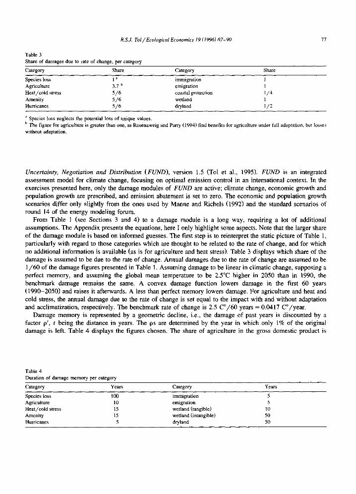
Fig. 2. Six scenarios for the change global mean surface air temperature, 1990-2100.

assumed to grow with the population and to fall with the growth of the economy. The valuation of intangible goods grows according to

GDP per capita

200OO GDP per capita '

1 + 200O0

implying that the maximum level is about twice as high as currently in the USA (cf., Manne et al., 1995). The number of people leaving is assumed to fall with

1

GDP per capita " 1 +

5O0

These assumptions are all rather ad hoc and serve for illustration only. Some sensitivity analysis is performed below.

Six temperature scenarios are investigated. In the first three, temperature rises linearly to 2.5, 3.5 and 4.5°(2 above 1990 levels, grossly corresponding to the IS92e, IS92b and IS92a (with high climate sensitivity) scenarios

0.0" k IS92a R E92b A C: IS92c

O.7- I~ exponential E ISO2e

~ 0,6" E triangular

B

01 ~ o.4-

1990 2000 2010 2020 2030 2040 2050 2060 2070 2080 2090 2100 year

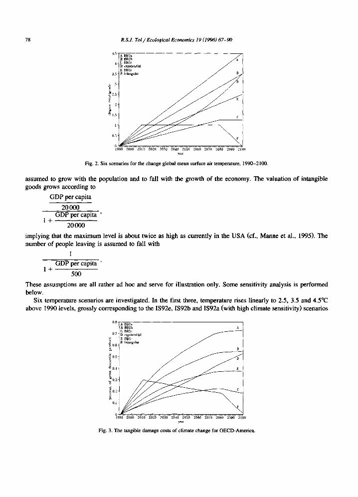
Fig. 3. The tangible damage costs of climate change for OECD-America.

R.S.J. Tol / Ecological Economics 19 (1996) 67-90

16 I ~: I I ] ~

oo

0",~ ....... ,,, . . . . . . . . . . . . . . . . . . . . , ....... ,,,, ,,,,,,,, . . . . . . . . . . . . . . . . . . . . . . . . . . . . . . . . . . . . . . . . "~1 1!1!111 2000 201[1 :2020 20:~1] :g{)lO 2050 20(;0 2070 2(;80 :!~9~) 21(10

yeal

Fig. 4. The intangible damage costs of climate change for OECD-America.

79

1.4 exponenlial N'q~e Irmngu~r

~ D

~ 0.6 -

i 0.4~

~'o.2=

oJ 199[) 2000 21110 2020 20011 2040 2050 2060 2070 2080 2090 21(111

)var

Fig. 5. The tangible damage costs of climate change for Africa.

~.5

! f 0 I ,,,,, . . . . . . . . . . . . . . . . . . . . . . . . . . . . . . . . . . . . . . . . . . . . . . . . . . . . . . . . . . . . . . . . . . . . . . . . . . . . . . . . . . . . . . . . . . . . . . . . . . . . . . . . 1990 2000 2010 2020 2030 2040 2050 3060 2070 200{I 2090 2100

year

Fig. 6. The intangible damage costs of climate change for Africa.


1.4-

.2.

0.8-

~ 0 . -

~ 0.4-

~" 0.2-

II

A: full d3~lamk~s R inclination to nugrate comtant

C

1990 2000 2010 :2020 20,qO 2010 2050 2060 .9070 .9080 2090 ~100 )car

Fig. 7. The sensitivity of the tangible damage costs for OECD-America to the dynamic specification.

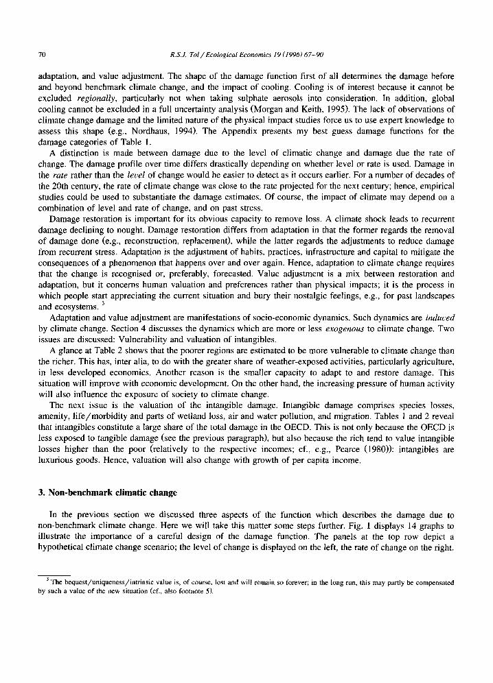
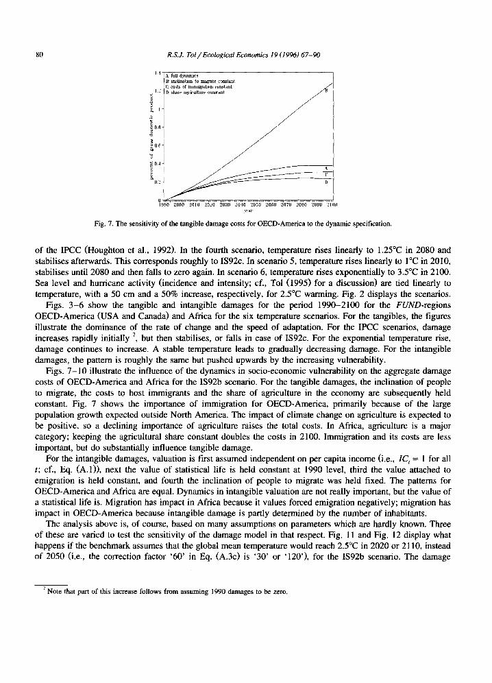
of the IPCC (Houghton et al., 1992). In the fourth scenario, temperature rises linearly to 1.25°C in 2080 and stabilises afterwards. This corresponds roughly to IS92c. In scenario 5, temperature rises linearly to I°C in 2010, stabilises until 2080 and then falls to zero again. In scenario 6, temperature rises exponentially to 3.5°C in 2100. Sea level and hurricane activity (incidence and intensity; cf., Tol (1995) for a discussion) are tied linearly to temperature, with a 50 cm and a 50% increase, respectively, for 2.5°C warming. Fig. 2 displays the scenarios.

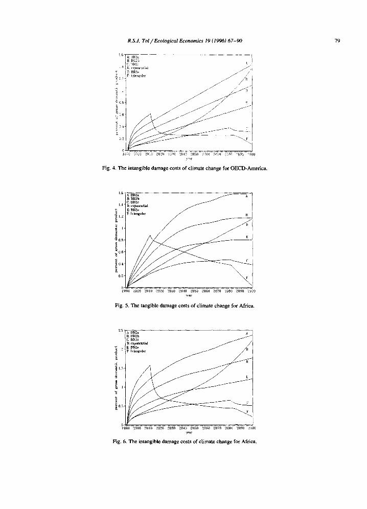
Figs. 3-6 show the tangible and intangible damages for the period 1990-2100 for the FUND-regions OECD-America (USA and Canada) and Africa for the six temperature scenarios. For the tangibles, the figures illustrate the dominance of the rate of change and the speed of adaptation. For the IPCC scenarios, damage increases rapidly initially 7, but then stabilises, or falls in case of IS92c. For the exponential temperature rise, damage continues to increase. A stable temperature leads to gradually decreasing damage. For the intangible damages, the pattern is roughly the same but pushed upwards by the increasing vulnerability.

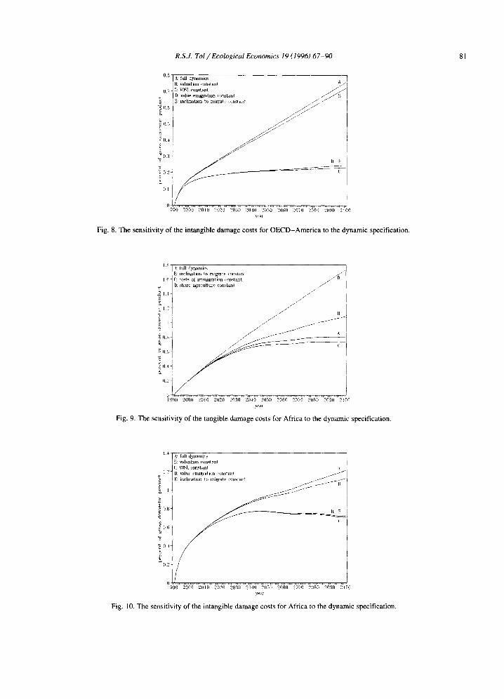
Figs. 7-10 illustrate the influence of the dynamics in socio-economic vulnerability on the aggregate damage costs of OECD-America and Africa for the IS92b scenario. For the tangible damages, the inclination of people to migrate, the costs to host immigrants and the share of agriculture in the economy are subsequently held constant. Fig. 7 shows the importance of immigration for OECD-America, primarily because of the large population growth expected outside North America. The impact of climate change on agriculture is expected to be positive, so a declining importance of agriculture raises the total costs. In Africa, agriculture is a major category; keeping the agricultural share constant doubles the costs in 2100. Immigration and its costs are less important, but do substantially influence tangible damage.

For the intangible damages, valuation is first assumed independent on per capita income (i.e., IC, = 1 for all t; cf., Eq. (A.1)), next the value of statistical life is held constant at 1990 level, third the value attached to emigration is held constant, and fourth the inclination of people to migrate was held fixed. The patterns for OECD-America and Africa are equal. Dynamics in intangible valuation are not really important, but the value of a statistical life is. Migration has impact in Africa because it values forced emigration negatively; migration has impact in OECD-America because intangible damage is partly determined by the number of inhabitants.

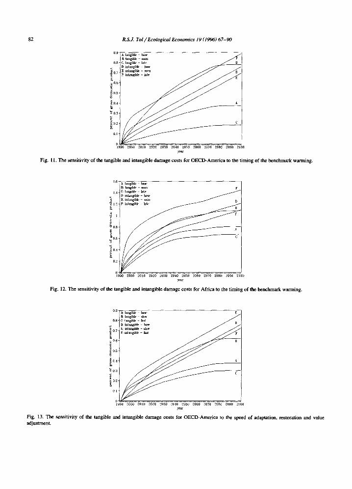
The analysis above is, of course, based on many assumptions on parameters which are hardly known. Three of these are varied to test the sensitivity of the damage model in that respect. Fig. 11 and Fig. 12 display what happens if the benchmark assumeS that the global mean temperature would reach 2.5°C in 2020 or 2110, instead of 2050 (i.e., the correction factor '60' in Eq. (A.3c) is '30' or '120'), for the IS92b scenario. The damage

7 Note that part of this increase follows from assuming 1990 damages to be zero.

R.S.J. Tel~Ecological Economics 19 (1996) 67-90 81

0.8-

0.7"

p 0.6 z.

05

0 .4"

full dynamic* ~aluation constant

C: VOSI, eol~stant [Y value emigl~ttion t'tlIIS[all{ E: inclination to migrate iiJnstani

= 0 . a t f I O. t

0 " ' ~ ~

- 0 1

1990 2000 2010 202-0 2030 2040 2t150 '21100 20T0 2080 :J090 2100 veal

Fig. 8. The sensitivity of the intangible damage costs for OECD-America to the dynamic specification.

1.0 i A: full dynamics I B: inelinalion to migrale ['OllSlant ~ ]

I 0 (': COSTS of i m m i g r a t i o n ca[as[ant .~ I'Z sham agriculture eonstanl

c 12

0 " -~ '

1.q00 2000 2.010 2020 2000 2040 2(150 200(I 2{170 2000 2090 210(I w,at

Fig. 9. The sensitivity of the tangible damage costs for Africa to the dynamic specification.

i l -

l .2-

k,

~ 0,8

~ 0 6 -

g 0.2 -

& full d y n a m i c s B: valuation ponstant C: VO81, mnst~ni ~, [}: vahle ellligratitJll eonslal)l /

i n c l i n a t i o n l o migra te eonslanl - zz ~990 2000 2010 2-020 2030 2-040 2050 2-068 2070 21/80 2-090 2100

year

Fig. 10. The sensitivity of the intangible damage costs for Africa to the dynamic specification.

82 R.S.J. Tol / Ecological Economics 19 (19961 67-90

0.9

tangible - soon ~ i " tangible - ba~

0.8 intangible - b a s e . . . . . , - 7 /

tangible - late

*~ intangible - soon / / / D ~ 0 . 7 ~ intengible - lat

~ 0.6 :g

0.5

0.4

o.,~

0.2

OA'

0 1990 2000 2010 2020 2030 21140 2050 2060 2070 2080 2090 2100

3~ar

Fig. 11. The sensitivity of the tangible and intangible damage costs for OECD-America to the timing of the benchmark warming.

1.6-

? ~ 1.2"

.~,

"~ 0.0-

~ 0.4"

0.2-

A: tangible - base [~ tangible - .~on F

: y , 0 .......................................... , , , ....... ,,,, ......... ,,, ....................................... 1990 2000 2010 2020 2030 2040 2050 2060 2070 2080 2090 2100

?,~ar

Fig. 12. The sensitivity of the tangible and intangible damage costs for Africa to the timing of the benchmark warming.

0.9"

0.6-

0.7-

.~ 0.6-

~ 0 . 0 -

1 0.4-

o.a-

~ 0.2-

0.1-

0

A~ tangible - base F, 1~ tangible - slow C: tangible - fast

I'~ intangible - shw J ~ / F: intangible - fast ~ / ~ ~ ~ F

1000 2000 2910 2020 2030 ~040 2050 2060 2070 2000 209(} 2100 veer

Fig. 13. The sensitivity of the tangible and intangible damage costs for OECD-America to the speed of adaptation, restoration and value adjustment.


1 . 4 ¸

1.2.

! 0 . 8

0.6.

0.4-

0.2"

D: tangible - slow E C: tangible - fast D g: intangible - l ~ e

intaagible - slow F F: intangible - f a s t

r

. . . . . . . . . . . . . . . H . . . . . . . . . . ......................................... . . . . . . . . . . . . . . . . . . . . . . . . . . . • 1990 2000 201U 2020 2030 2040 2050 2960 2070 20Bf~ 2090 2100

veal"

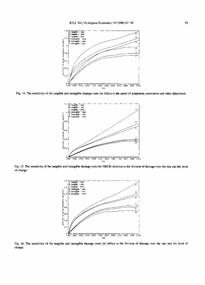
Fig. 14. The sensitivity of the tangible and intangible damage costs for Africa to the speed of adaptation, restoration and value adjustment.

1.2"

.2 0.8"

k tangible - base R tangible - rate C: tangible - level F / 1~ intangible - base Fz ilflangible - rate F: intangible - level

0

~ 0.6" i

o.4.

~,o2

o . . . . . . . . . . . . . . , H . . . . . . . . . . . . . . . . . . . . . . . . . . . . . . . . . . . . . . . . . . . . . . . . . . . . . . . . . . . . . . . . . . . . . . . . . . . . . . . . . . . . . . . 1990 2060 2010 2020 2030 2046 ~050 2060 ?070 2080 2090 2100

y~'ar

Fig. 15. The sensitivity of the tangible and intangible damage costs for OECD-America to the division of damage over the rote and the level of change.

l.fi ~ tangible - ha,c,

[~ tangible - tale J ~ , ~ [ .4- C: tangible - levH

I~ intangible - base f / I~ intangible - rate / l) ~ 1.2- F: intangible - level

~ 0.8- A

0 . 6 -

~ 0 . 4 -

0.2-

0 .................................................................................. , ....... , ................. 1990 2000 2010 2020 ~030 2040 20,50 2(t60 2070 2OBO 2090 2100

year

Fig. 16. The sensitivity of the tangible and intangible damage costs for Africa to the division of damage over the rate and the level of change.


profiles remain qualitatively the same. Interestingly, damage reacts about twice as strong to putting the benchmark more upfront, than to delaying it. Fig. 13 and Fig. 14 display the sensitivity to the speed of adaptation; restoration; value adjustment. The Ps, see Eq. (A.2), now follow from assuming that 0.1% or 10% (base case: 1%) of the initial damage remains after the life-times of Table 4. Again, the damage profiles qualitatively remain the same. Fig. 15 and Fig. 16 display what happens in case all damages associated with rate and level of change s are assumed to be completely due to rate of level. The qualitative damage profiles do not change. Damage goes up in case it is due to the level of change. The downward reaction of tangible damage is stronger than the upward; this is reversed for intangible damages.

The analyses in this section demonstrate the importance of a dynamic specification of climate change damage costs. The presence of dynamic features is tentatively shown to be more important than the choice of parameters of the damage model proposed in the Appendix.

6. Uncertainty

Uncertainty abounds in climate change issues! Our knowledge on all main processes, climate change, its physical impact and the economic damage, is far from complete. In addition, the uncertainty cascades through a number of levels (Shlyakhter et al., 1994). In Tol (1995), I looked at this issue through convolutions of conditional probability distributions, assuming that decision makers are interested in the expected damages and even more so in the expected reduction of the damage given (i.e., conditional upon) the proposed abatement measures. The damage costs discussed in the above all reflect best guesses, here interpreted as the mode of the distribution describing the uncertainty conditional upon the mode of the process causing the damage. For example, damage D is induced by a change in the global mean temperature T, following some function f(T) and with probability distribution p(D =f(T)) . But T is uncertain itself, leading to the natural interpretation of p(D) as conditional on T. Thus, the parameter of interest D follows a convoluted distribution.

A convoluted probability distribution is fatter tailed than its components, that is, the uncertainty increases. In climate change issues, the expected damage is further enlarged because of the prevalence of positive skewness in the uncertainties and the many convex transformations between the levels. Countervailing these three factors of ever increasing uncertainties is the portfolio effect: As climate change is regionally and sectorally diversified, bad luck in one place is compensated for by good luck elsewhere, thereby reducing the overall uncertainty. Some simple numerical examples, reported in Tol (1995), show that this effect is minor compared to the others: Expected damages can be up to a factor fifty larger than the best guesses. This study is of limited evidence as both the numbers of levels of uncertainties (3 at most) and the number of regions (9) and impact categories (9) are small. It does, however, demonstrate the dominance of convolution over portfolio.

This reasoning also applies through time. The future depends on the present so the future uncertainties are conditional upon the present ones. The unconditional uncertainties are hence convolutions of present and future uncertainties, and larger than the conditional uncertainties. Little to no attention has been paid to the implications of this for modelling and policy, at least, in my knowledge.

Learning, and particularly how it affects optimal emission reduction paths is subject of much study (e.g., Kolstad, 1994; Manne and Richels, 1992; Nordhaus, 1994; Ulph and Ulph, 1994). However, this literature focuses on the unrealistic case of full uncertainty resolution. Partial resolution and increases of uncertainty receive little or no attention.

8 Except agriculture, heat stress and cold stress, where there is a basis in the underlying studies for distinguishing between rate and level.


7. Higher order damage

I now have tentatively derived a dynamic set of climate change damage categories and functions. The economy is confronted with this set. Climate change damages set a chain of other effects in motion. For instance, coastal defence commonly is considered a government's task. Increased government spending on this part inevitably leads to either reduced spending elsewhere, or tax, deficit or inflation increases. Reductions in agricultural yield imply price increases. This type of reasoning holds for each damage category. The macroeconomic impacts of small changes to not too significant sectors are likely to be small. More important sectors, larger direct changes and compound effects may add substantially to the total damage costs, however. For instance, the insurance and reinsurance sector is the first buffer for the material Consequences of extreme weather events. Other sectors face huge costs should this buffer fail. The (re)insurance sector ran into big trouble in the early 1990s as a consequence of a series of severe hurricanes and storms; the reaction of the sector consisted mainly of restricted cover and raised premiums (Tol, 1996; Tol and Leek, 1996). Many activities, e.g., mortgaging, are performed under the assumption that there is insurance and so little risk. Being confronted with unexpected losses is a problem, as is investing without proper insurance.

The issue here is the manner in which the physical and economic damages themselves propagate, The first and foremost questions are, of course: Do they propagate? And, if so: What is the order of magnitude? The first question is easily answered in the affirmative. In a complex system such as the economy in which everything is linked to everything, every shock propagates through the entire system. The suitable question is therefore: Is the order of magnitude greater than the system's noise level? Scheraga et al. (1993) attempt to answer such questions with a dynamic general equilibrium model of the USA. Although they do calculate through the impact on agricultural, coastal protection and electricity consumption, they omit to compare the costs of climate change in a general equilibrium setting with the costs in partial equilibrium. Their results do show a certain synergy in the economic effect: The costs of impacts together is larger than the sum of the individual impacts.

In general, if the environment declines, more defensive expenditures need to be made. Defensive investment is here the expenditure on durable goods which only serve to help common (productive) capital goods function properly. The distinction between defensive and productive capital goods and investment is highly artificial, but the intuitive appeal is clear: Dikes, say, are not productive; without them, the plants behind them would not be either. An example of defensive consumption is insurance. If defensive expenditures are forced to rise, consumptive and productive expenditures fall, because of finite budgets. Under neo-classical assumptions, consumption and production fall to the point where their marginal utilities equal those of the defensive expenditures. How to measure the consumption loss is the same question which is attempted to be answered by the numerous correction methods for gross domestic product (Ref. to Harmen). These problems are outside the scope of this paper. In case defensive and productive capital goods are not separated (they are not in standard accounts), the shift from productive to defensive investment reveals itself in a lower capital productivity coefficient.

In the previous paragraph, I mentioned in passing that the marginal utility of defensive consumption and investment ought to be equal to the marginal utility of common consumption and productive investment, in order to obtain an optimal allocation of means. This supposes perfect information, which is a rather strong assumption with regard to climate change. This implies that defensive investment will be too high in some places (a suboptimal use of scarce resources) and too low in others (unduly high losses). The extent to which this will occur depends on both the rate of change and the forecastibility.

The uncertainties accompanying climatic change induce another cost not assessed so far in the literature. It has been argued above that uncertainty itself is a reason for greenhouse gas emission abatement. The same argument is used in project evaluation. The greater the risk, the greater the required rate of return. Climatic change increases the overall risk, but particularly in some sectors, such as agriculture, and hence lowers the overall investment, but in particular shifts capital from some sectors to other, less risky ones. This is a part of adaptation, lowering the costs of climate change.


8. Condu~ons

Any model is better than no model, provided its assumptions are clearly stated and the mapping from assumptions to results is clear. This paper presents a model of the damage costs of climate change, dynamic in both climate and socio-economic vulnerability. The model serves three purposes. Firstly, it is the experimental damage module of FUND, an integrated assessment model of climate change of the cost-benefit type. Secondly, a formal model helps to structure, hopefully, not only my thinking but also the debate. Thirdly, the present functional forms are intended to point climate change impact analysts at the sensitivity of damage estimates so as to urge them to work on more proper reduced forms.

In a series of steps, the paper argues qualitatively and quantitatively that the manner in which the dynamics of both climate and socio-economic vulnerability affect the impacts of the enhanced greenhouse effect matters a great deal. This calls for a reexamination of the current generation of damage models and damage modules in integrated assessment models. It also calls for research programme to replace my 'expert' judgement by more thorough analysis.

Acknowledgements

This paper would not have been the same without the constructive discussions with and extensive comments of Sam Fankhauser, Reyer Gerlagh, Matthijs HisschemiSller, Huib Jansen, Steve Schneider, Pier Vellinga, Harmen Verbruggen and the participants of the Nato Advanced Research Workshop on the economics of air pollution, Wageningen, 16-18 November, 1994. I hereby express my thanks to them and to the Dutch National Research Programme: Global Air Pollution and Climate Change for partly funding this research under grant 8510855.

Appendix A. Experimental damage cost module of the climate framework for uncertainty, negotiation and distribution, version 1.5

IC t, the factor with which the intangible losses are increased follows

YpC t 1 + YpC0/20000 IC t -- , (A.1)

1 + YpCt/20000 YpC 0

where YpC is the income per capita. The loss of species, ecosystems and the like, C s is modelled as

sL l cSt = N Yt l Ct" ~ "-~o + t - ~ o ] ] + Ps , - , ,

where SC is the species loss coefficient in fraction of GPD of Table 2, divided by 60 to go from the level to the rate of change.

Human amenity follows

C A = cA,L + C A,R, (A.3a)

where 1 T , - T o

cA,L = --A Y t l C t ~ (A.3b) 6 To

and

cA ,R = - - r, ic, - aT0 vA , - ' , . 6 60 [ ~ + (A.3c)

R.S.J. Tol / Ecological Economics 19 (1996) 67-90 8 7

The number of deaths D u related to heat stress follows a similar pattern

Ot n = Ot n'L + Ot n'R, (A.4a)

where

1 ~ - T o D~ "L = - H P , , (A.4b)

6 T O

with P the population and

D~'R=--660--P'~ - ~ o + Ar°] I t'D , - , " (A.4c)

The number of deaths related to cold stress D c follows an identical scheme with different parameters. The costs C "c follow from

O, nc = VHL,( O~ + O c) + PL Off c , , (A.4d)

where

VHL, = 250000 + 175YpC t. (A.5)

Agricultural damage D Agf is supposedly equal to

Ct agr= C Agr'L -+- C Agr'R, (A.6a)

where

7",-To C Agr'L = Agr e Yt A g f - (A.6b)

To and

P ' A g r ~ " t - 1 " c~g~'R=AgrRy g - ~ l - ~ o + + (A.6c)

Hurricane damage is

Ct Hr = C Hr'L + Ct Hr'R, (A.7a)

where

1 HA t - HA o C Hr'L = ~ H r r t HAo , (A.7b)

with HA the hurricane activity and

-~-~Yt-~ AHA----~ + AHA o] ] if A H A , > 0 ctHr,R _ cHr R (A.7c)

= Pm ,-'l +

5 6 -~Yt~ AHA--------~ + A---~0 ] ] if A H A t < 0

Hurricane activity lumps together intensity, frequency and geographical spread. All could change, though no one knows how (Kattenberg et al., 1996). Damage characteristics would be very different. However, one indicator is chosen for convenience. Once climatologists come up with clearer indications as to future hurricane regimes, Eq. (A.7) needs to be reconsidered.


The number of additional deaths due to hurricane activity exactly mirrors Eq. (A.7); the costs follow from multiplication by Eq. (A.5).

The number of people forced to migrate is

L l + YPCo/500 [ASL,[ P L , = 6--6 1 + YPCr/500 Pt 0.0-----~' (A.8a)

where SL is the sea level. The term in YpC is a logistic adjustment to vulnerability, similar, but reversed, to Eq. (A.1). The costs of people leaving is then

C, L = PLt3YpC , + PLCL1 (A.8b)

and the costs of people in region j entering

DtZj = 0.4YpC,4 y" tzijPL,.i + PECE-' ' (A.8c) i

where ~ij is the fraction of people leaving region i that enter region j. The costs of coastal protection are

c5 P = c P,L + c5

where

1 SL t - SL o C CP'L = -CPY,

4 SL o

and

where

3 CP 1 I ASTI ( AS t 2

cCP,R = - cCP,R PCP t-l + 1 3 CP Yt 1.2 (]AIStl + (ZlSt) 2)

5 4 6 0 1 " ~ - 0 ~AS 0

and

The costs of dryland loss follow

~ L = ~ L , L + ~L,R,

1 S L t - SL 0 ctOL. L = _ DLY,

2 SL 0

Ct Cp,R = PDLCD_L1 'R + [ -- __ _ _

,oL 2) + aSo

1 1 D L 1 [lASt , ( A S , ) 2)

if AS, > 0

if ASt < 0

if AS l > 0

if AS, < 0

(A.9a)

(A.9b)

(A.9c)

(A.10a)

(A.9b')

(A.9c')


The tangible costs of wetland loss are

2 60 AS o c W L ~T WL ,T

= P W L ' T C t I + 1 1 W L y t l ( I A S t l

5 2 60 - ~ o +

and the intangible costs of wetland loss

cy ,, = pw ,,c,w ., +

AS ° if AS, > 0

,aSo ] j

- - + if AS, > 0 2 60 AS o ~ AS o

5 2 60 t +,-o if AS, < O

(A.11a)

(A.11b)

R e f e r e n c e s

Burton, I., Kates, R,W. and White, G.F., 1993. At Risk: Natural Hazards, People's Vulnerability and Disasters. Routledge, London. Cline, W.R., 1992. The Economics of Global Warming. Institute for International Economics, Washington, DC. Dowlatabadi, H, and Morgan, G., 1993. A model framework for integrated studies of the climate problem. Energ. Policy, 15: 2(/9-221. Fankhauser, S., 1995. Valuing Climate Change: The Economics of the Greenhouse. EarthScan, London. Hanemann, W.M., 1991. Willingness to pay and willingness to accept: How much can they differ? Am. Econ. Rev., 81: 635-647. Hope, C.W., Anderson, J. and Wenman, P., 1993. Policy analysis of the greenhouse effect: An application of the PAGE model. Energ.

Policy, 15: 328-338. Houghton, J.T., Callander, B.A. and Varney, S.K., 1992. Climate Change 1992: The Supplementary Report of the IPCC Scientific

Assessment. Cambridge University Press, Cambridge. Hoel, M. and Ivaksen, I., 1993. The Environmental Costs of Greenhouse Gas Emissions. Mimeo, University of Oslo. Kalkstein, L.S., 1989. The impact of CO 2 and trace-gas induced climate changes upon human mortality, In: ed. J.B. Smith and D.A. Tirpak,

The Potential Effects of Global Climate Change on the United States, Appendix G: Health. Environmental Protection Agency, Washington, DC.

Kalkstein, L.S., 1993. Health and climate change: Direct impact in cities. Lancet, 342: 1397-1399. Kattenberg, A., Giorgi, F., Grassl, H., Meehl, G.A., Mitchell, J.F.B., Stouffer, R.J., Tokioka, T., Weaver, A.J. and Wigley, T.M.L.. 1996.

Climate models - projections on future climates. In: eds. J.T. Houghton, L.G. Meiro Filho, B.A. Callander, N. Harris, A. Kattenberg and K. Maskell, Climate Change 1995: The Science of Climate Change - Contribution of Working Group I to the Second Assessment Report of the Intergovernmental Panel on Climate Change. Cambridge University Press, Cambridge.

Kolstad, C.D., 1994. George Bush versus A1 Gore: Irreversibilities in greenhouse gas accumulation and emission control investment. Energ. Policy, 22: 772-778.

Manne, A.S., Mendelsohn, R. and Richels, R.G., 1995. MERGE: A model for evaluating regional and global effects of GHG reduction policies. Energ, Policy, 23: 17-34.

Manne, A.S. and Richels, R.G., 1992. Buying Greenhouse Insurance: The Economic Costs of CO 2 Emission Limits. MIT Press, Cambridge. MA.

Morgan, M.G. and Keith, D.W., 1995. Subjective Judgments by Climate Experts. Environ. Sci. Technol., 29: 468A-476A. Nordhaus, W.D., 1991. To slow or not to slow: The economics of the greenhouse effect. Econ. J., 101 :, 920-937. Nordhaus, W.D., 1994. Managing the Global Commons: The Economics of Climate Change. MIT Press, Cambridge, MA. Parry, I.W.H., 1993. Some estimates of the insurance value against climate change from reducing greenhouse gas emissions. Resour. Energ.

Econ., 15:, 99-115. Pearce, D.W., 1980. The social incidence of environmental costs and benefits. In: ed. T. O'Riordon and R.K. Turner, Progress in Resource

Management and Environmental Planning. John Wiley and Sons, Chichester. Pearce, D.W., Achanta, A.N., Cline, W.R., Fankhauser, S., Pachauri, R., Tol, R.S.J. and Vellinga, P., 1996. The social costs of climate

change: Greenhouse damage and the benefits of control. In: ed. J.P. Bruce, H. Lee and E.F. Haites, IPCC WGIII Second Assessment Report. Cambridge University Press, Cambridge, forthcoming.

90 R.S.Z Tol / Ecological Economics 19 (1996) 67-90

Peck, S.C. and Teisberg, T.J., 1994. Optimal carbon emissions trajectories when damages depend on the rate or level of global wanning. Clim. Change, 28: 289-314.

Rosenzweig, C. and Parry, M.L., 1994. Potential impact of climate change on world food supply. Nature, 367: 133-138. Scheraga, J.D., Leary, N.A., Goettle, R.J., Jorgenson, D.W. and Wilcoxen, P.J., 1993. Macroeconomic modeling and the assessment of

climate change impacts. In: ed. Y. Kaya, N. Nakicenovic, W.D. Nordhaus and F.L., Toth, Costs, Impacts and Benefits of CO 2 Mitigation. IIASA Collaborative Paper Series CP-93-2, Laxenburg.

Shlyakhter, A.I., Valverde A., L.J., Jr. and Wilson, R., 1994. Integrated Risk Analysis of Global Climate Change. Mimeo, Harvard University.

Sztrepek, K.M. and Smith, J.B., eds., 1995., As Climate Changes. Cambridge University Press, Cambridge. Titus, J.G., 1992. The costs of climate change to the United States. In: ed. S.K. Majumdar, L.S. Kalkstein, B. Yamal, E.W. Miller and L.M.

Rosenfeld, Global Climate Change: Implications, Challenges and Mitigation Measures. Pennsylvania Academy of Science. Tol, R.S.J., 1994. The damage costs of climate change: A note on tangibles and intangibles, Applied to DICE. Energy Policy, 22: 436-438. Tol, R.S.J., 1995. The damage costs of climate change toward more comprehensive calculations. Environ. Resour. Econ., 5: 353-374. Tol, R.S.J., 1996. The weather insurance sector. In: ed. T.E. Downing, A.A. Olsthoorn and R.S.J. Tol, Climate Change and Extreme Events:

Altered Risk, Socio-economic Impacts and Policy Responses. Institute for Environmental Studies R96/04, Vrije Universiteit, Amsterdam.

Tol, R.S.J., Van der Burg, T., Jansen, H.M.A. and Verbruggen, H., 1995. The Climate Fund: Some Notions on the Socio-economic Impacts of Greenhouse Gas Emissions and Emission Reduction in an International Context. R95/03, Institute for Environmental Studies, Vrije Universiteit, Amsterdam.

Tol, R.S.J. and Leek, F.P.M., 1996. Economic approaches to natural disasters. In: ed. T.E. Downing, A.A. Olsthoorn and R.S.J. Tol, Climate Change and Extreme Events: Altered Risk, Socio-economic Impacts and Policy Responses. Institute for Environmental Studies R96/04, Vrije Universiteit, Amsterdam.

Ulph, A. and Ulph, D., 1994. Global Warming, Irreversibility, and Learning: Some Clarificatory Notes. Mimeo, University of Southampton and University College London.

Weyant, J.P., Cline, W.R., Davidson, O., Dowlatabadi, H., Edmonds, J.A., Fankhauser, S., Grubb, M.E., Richels, R.G., Rotmans, J. and Tol, R.S.J., 1996. Integrated assessment of climate change. In: ed. J.P. Bruce, H. Lee and E.F. Haites, IPCC WGIII Second Assessment Report. Cambridge University Press, Cambridge, forthcoming.

Yohe, G., Neumann, J. and Ameden, H., 1995. Assessing the economic cost of greenhouse-induced sea level rise: Methods and applications in support of a national survey. J. Environ. Econ. Manage., 29: $78-$97.