


Bahasa
Halaman
Hukum

DataCamp Survival Analysis in R
The Cox Model
SURVIVAL ANALYSIS IN R
Heidi SeiboldStatistician at LMU Munich
DataCamp Survival Analysis in R
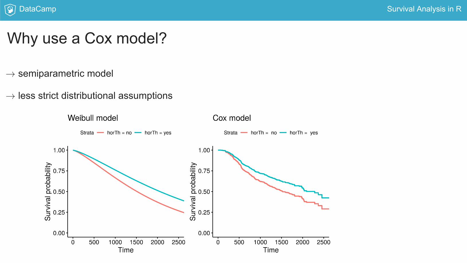
Why use a Cox model?
→ semiparametric model
→ less strict distributional assumptions

DataCamp Survival Analysis in R
The proportional hazards assumption
Not possible:

DataCamp Survival Analysis in R
Computing the Cox model
Cox model:
Weibull model:
cxmod <- coxph(Surv(time, cens) ~ horTh, data = GBSG2)
coef(cxmod)
#> horThyes
#> -0.3640099
wbmod <- survreg(Surv(time, cens) ~ horTh, data = GBSG2)
coef(wbmod)
#> (Intercept) horThyes
#> 7.6084486 0.3059506

DataCamp Survival Analysis in R
Let's practice computingCox models
SURVIVAL ANALYSIS IN R
DataCamp Survival Analysis in R
Visualizing the Cox model
SURVIVAL ANALYSIS IN R
Heidi SeiboldStatistician at LMU Munich
DataCamp Survival Analysis in R
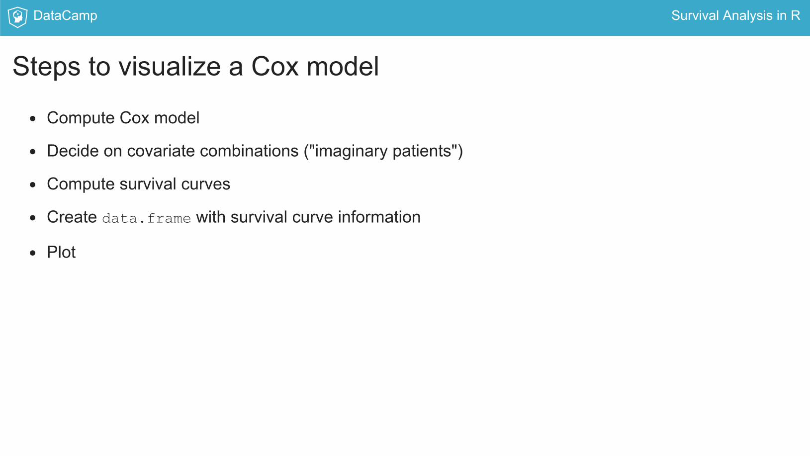
Steps to visualize a Cox model
Compute Cox model
Decide on covariate combinations ("imaginary patients")
Compute survival curves
Create data.frame with survival curve information
Plot
DataCamp Survival Analysis in R
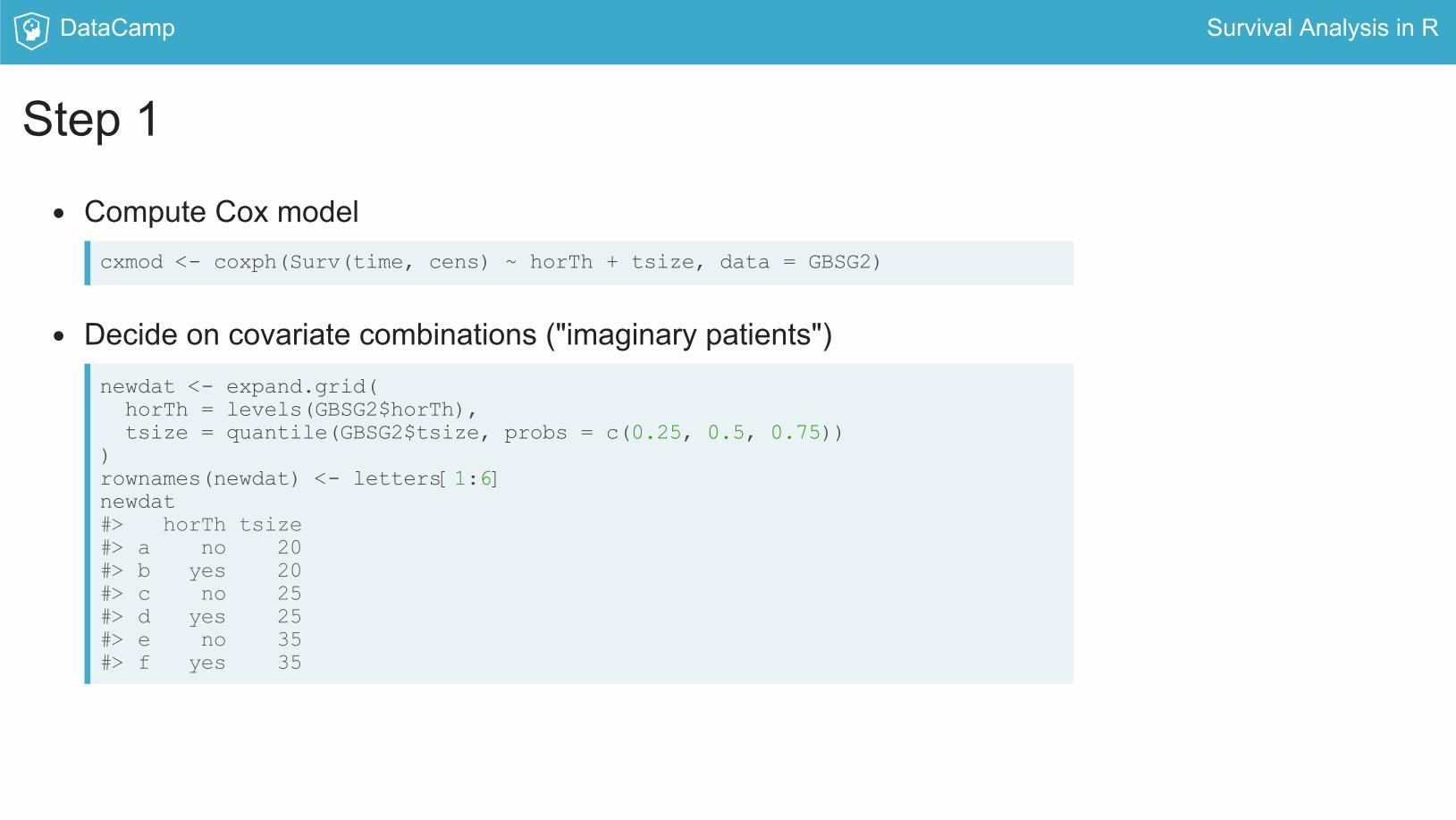
Step 1
Compute Cox model
Decide on covariate combinations ("imaginary patients")
cxmod <- coxph(Surv(time, cens) ~ horTh + tsize, data = GBSG2)
newdat <- expand.grid(
horTh = levels(GBSG2$horTh),
tsize = quantile(GBSG2$tsize, probs = c(0.25, 0.5, 0.75))
)
rownames(newdat) <- letters[1:6]
newdat
#> horTh tsize
#> a no 20
#> b yes 20
#> c no 25
#> d yes 25
#> e no 35
#> f yes 35
DataCamp Survival Analysis in R
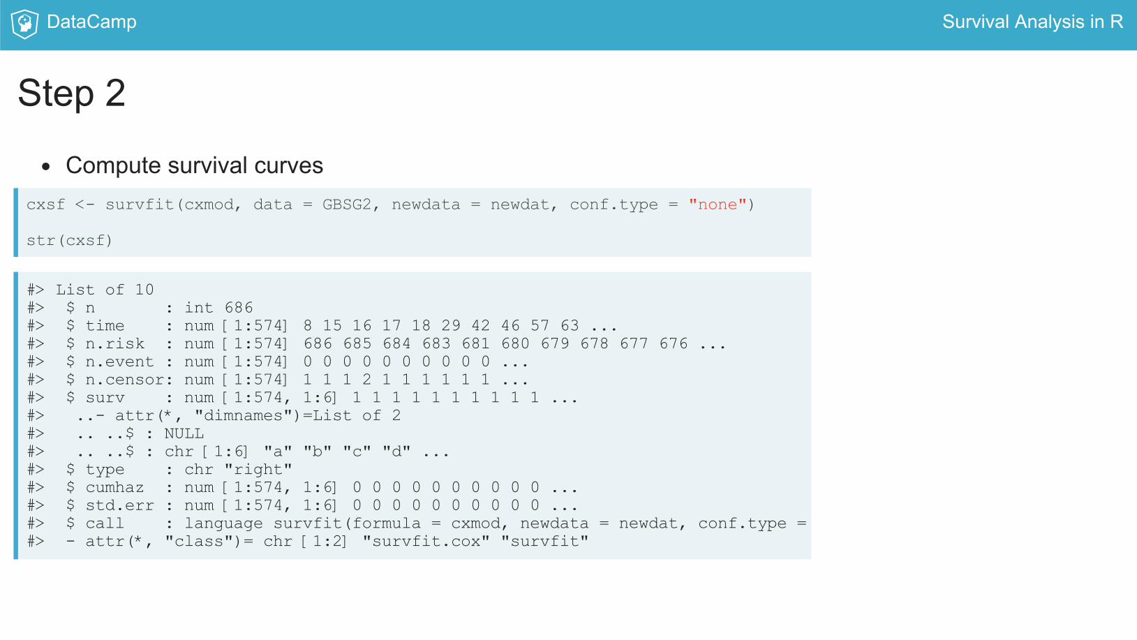
Step 2
Compute survival curvescxsf <- survfit(cxmod, data = GBSG2, newdata = newdat, conf.type = "none")
str(cxsf)
#> List of 10
#> $ n : int 686
#> $ time : num [1:574] 8 15 16 17 18 29 42 46 57 63 ...
#> $ n.risk : num [1:574] 686 685 684 683 681 680 679 678 677 676 ...
#> $ n.event : num [1:574] 0 0 0 0 0 0 0 0 0 0 ...
#> $ n.censor: num [1:574] 1 1 1 2 1 1 1 1 1 1 ...
#> $ surv : num [1:574, 1:6] 1 1 1 1 1 1 1 1 1 1 ...
#> ..- attr(*, "dimnames")=List of 2
#> .. ..$ : NULL
#> .. ..$ : chr [1:6] "a" "b" "c" "d" ...
#> $ type : chr "right"
#> $ cumhaz : num [1:574, 1:6] 0 0 0 0 0 0 0 0 0 0 ...
#> $ std.err : num [1:574, 1:6] 0 0 0 0 0 0 0 0 0 0 ...
#> $ call : language survfit(formula = cxmod, newdata = newdat, conf.type =
#> - attr(*, "class")= chr [1:2] "survfit.cox" "survfit"

DataCamp Survival Analysis in R
Step 3
Create data.frame with survival curve informationsurv_cxmod0 <- surv_summary(cxsf)
head(surv_cxmod0)
#> time n.risk n.event n.censor surv std.err upper lower strata
#> 1 8 686 0 1 1 0 NA NA a
#> 2 15 685 0 1 1 0 NA NA a
#> 3 16 684 0 1 1 0 NA NA a
#> 4 17 683 0 2 1 0 NA NA a
#> 5 18 681 0 1 1 0 NA NA a
#> 6 29 680 0 1 1 0 NA NA a
surv_cxmod <- cbind(surv_cxmod0,
newdat[as.character(surv_cxmod0$strata), ])
DataCamp Survival Analysis in R
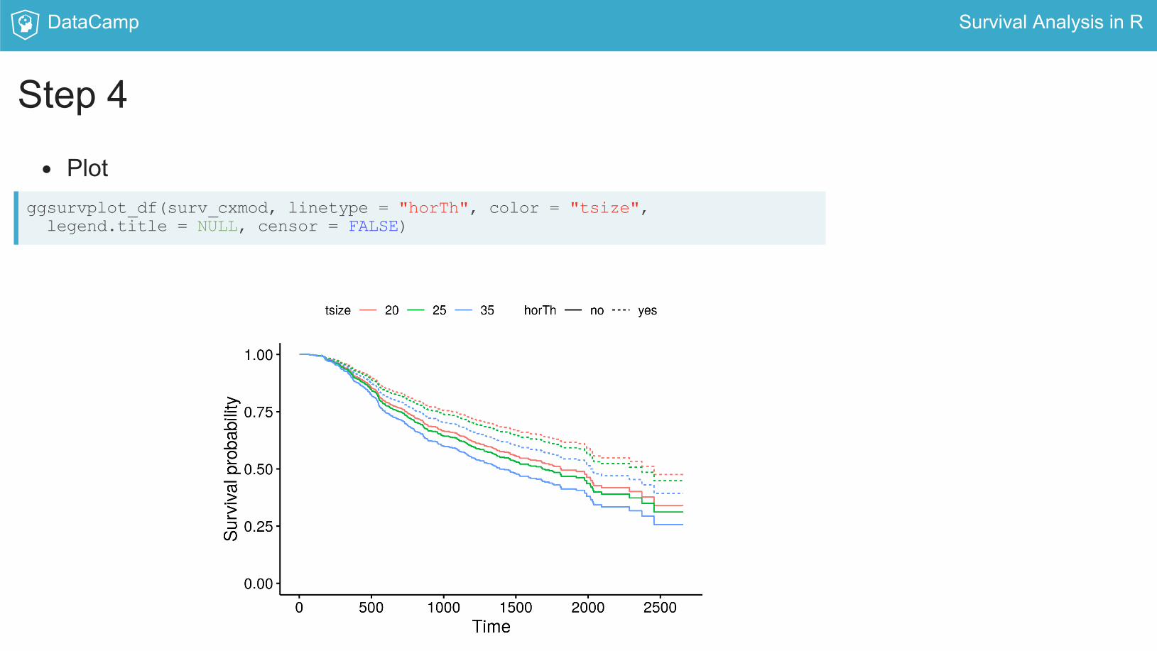
Step 4
Plotggsurvplot_df(surv_cxmod, linetype = "horTh", color = "tsize",
legend.title = NULL, censor = FALSE)

DataCamp Survival Analysis in R
Now it's your turn tovisualize!
SURVIVAL ANALYSIS IN R

DataCamp Survival Analysis in R
What we've learned in thiscourse
SURVIVAL ANALYSIS IN R
Heidi SeiboldStatistician at LMU Munich

DataCamp Survival Analysis in R
Concepts and Methods
CONCEPTS
Why survival methods
Censoring
Survival curve
METHODS
Kaplan-Meier Estimate
Weibull model
Cox model
DataCamp Survival Analysis in R
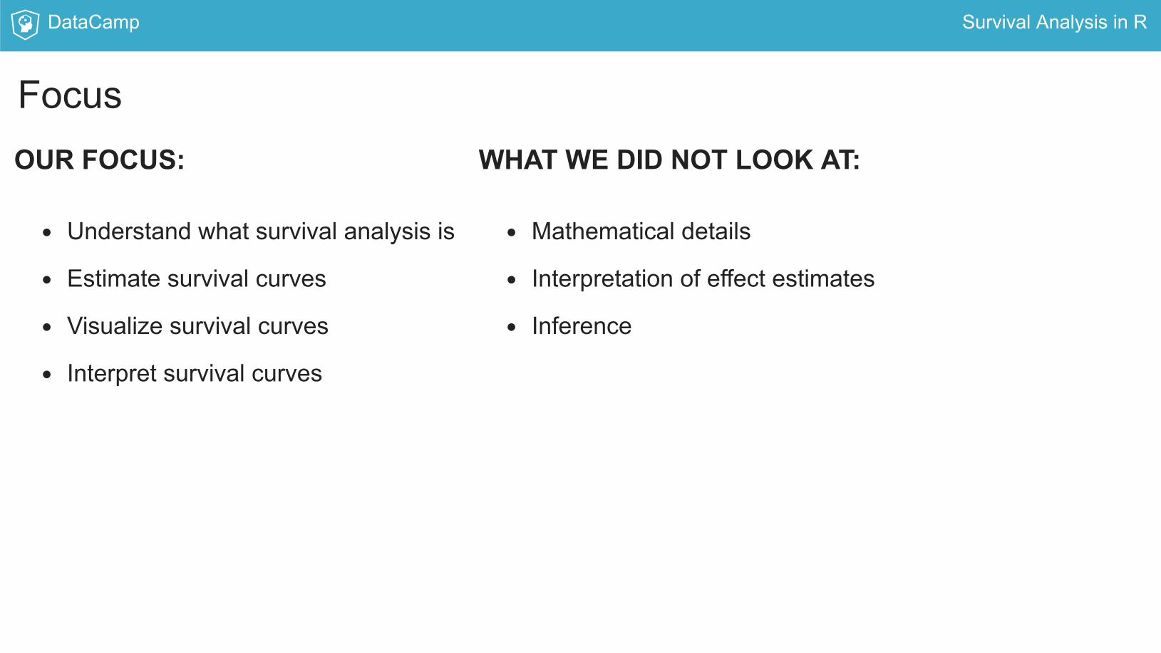
FocusOUR FOCUS:
Understand what survival analysis is
Estimate survival curves
Visualize survival curves
Interpret survival curves
WHAT WE DID NOT LOOK AT:
Mathematical details
Interpretation of effect estimates
Inference

DataCamp Survival Analysis in R
Let's practice one moretime!
SURVIVAL ANALYSIS IN R

DataCamp Survival Analysis in R
Thanks and Good Bye
SURVIVAL ANALYSIS IN R
Heidi SeiboldStatistician at LMU Munich

DataCamp Survival Analysis in R
Where you can go from here
Learn about...
What do the model estimates mean?
Tests, confidence intervals
Mathematical background
Competing risks models and other more advanced models
Other R packages
DataCamp Survival Analysis in R
Have fun!
SURVIVAL ANALYSIS IN R
Copyright © 2022 FDOKUMEN

