Download - Spatial aspects of the design and targeting of agricultural development strategies

EPTD DISCUSSION PAPER NO. 44

Environment and Production Technology Division

International Food Policy Research Institute (IFPRI)2033 K Street, N.W.

Washington, D.C. 20006

May 1999

EPTD Discussion Papers contain preliminary material and research results, and arecirculated prior to a full peer review in order to stimulate discussion and critical comment. Itis expected that most Discussion Papers will eventually be published in some other form, andthat their content may also be revised.

SPATIAL ASPECTS OF THE DESIGN AND TARGETINGOF AGRICULTURAL DEVELOPMENT STRATEGIES

Stanley Wood, Kate Sebastian, Freddy Nachtergaele,Daniel Nielsen, and Aiguo Dai

ABSTRACT

Two increasingly shared perspectives within the international developmentcommunity are that (a) geography matters, and (b) many government interventions wouldbe more successful if they were better targeted. This paper unites these two notions byexploring the opportunities for, and benefits of, bringing an explicitly spatial dimensionto the tasks of formulating and evaluating agricultural development strategies.

The paper was originally conceived to address the more specific goal of proposinga spatial characterization to underpin deliberations on appropriate development strategiesfor the “fragile” or “less-favored” lands of Sub-Saharan Africa. In practice, however, weconsidered that goal to be not only impractical but, perhaps, ill-conceived. The multiplesenses in which land may be considered fragile, coupled with the myriad of potentialdevelopment pathways would result in either an overly complex characterization or, morelikely, a need to aggregate and generalize that would render the characterization of littleuse when confronted with any specific, real-world problem. We first review the linguafranca of land fragility and find it lacking in its capacity to describe the dynamic interfacebetween the biophysical and socioeconomic factors that help shape rural developmentoptions. Subsequently, we propose a two-phased approach. First, development strategyoptions are characterized to identify the desirable ranges of conditions that would mostfavor successful strategy implementation. Second, those conditions exhibiting importantspatial dependency – such as agricultural potential, population density, and access toinfrastructure and markets – are matched against a similarly characterized, spatially-referenced (GIS) database. This process generates both spatial (map) and tabularrepresentations of strategy-specific development domains.

While there are many advantages to this tailored approach, it does depend onhaving access to a modest GIS capacity to re-characterize and re-interpret spatial datasetsas the nature and focus of development problems change, and as new and improved databecome available. This would be a significant step for many policy analysis units,typically run by economists. However, while acknowledging that not all aspects ofstrategic analysis necessarily benefit from a spatial perspective, we feel an importantadditional benefit of a spatial (GIS) framework is that it provides a powerful means oforganizing and integrating a very diverse range of disciplinary and data inputs.

At a more conceptual level we propose that it is the characterization of location,not the narrowly-focused characterization of land, that is more properly the focus ofattention from a development perspective. IFPRI is expanding on these concepts in itswork on policy-relevant applications of GIS linked more closely to economic perceptionsof space.

The paper includes appropriate examples of spatial analysis using data from EastAfrica and Burkina Faso, and concludes with an appendix describing and interpretingregional climate and soil data for Sub-Saharan Africa that was directly relevant to ouroriginal goal.

i

CONTENTS

1. Introduction....................................................................................................................1

2. Issues, Concepts, and Methods ......................................................................................5Paradigms for Relating Livelihoods and Landscapes....................................................5Land and Location .........................................................................................................8

The Lingua Franca of Land Fragility.......................................................................8Confusing Land with Location ................................................................................9Location and Time .................................................................................................13

Generic Characterization: Problematic, Restrictive and Unnecessary.........................15Spatial Analysis Techniques ........................................................................................18

Visualization ..........................................................................................................19Intersection.............................................................................................................19Spatial Characterization .........................................................................................19Distance and Network Functions ...........................................................................20Spatial Relationships..............................................................................................20

Development Strategy Applications of Spatial Analysis.............................................21Problem Diagnosis .................................................................................................21Development Strategy Characterization and Evaluation .......................................28Benchmark Sites and Extrapolation Domains .......................................................50

3. Conclusions..................................................................................................................51

References..........................................................................................................................56

Appendix: A Regional Overview of Climate, Soil, and Terrain Conditionsand Datasets for Sub-Saharan Africa.................................................................................63

Rainfall.........................................................................................................................63Annual Rainfall Patterns and Seasonal Variations ................................................63Long-Term Rainfall Trends ...................................................................................65Outlook for Near-Future Temperature and Rainfall ..............................................67

Soil and Terrain Data ...................................................................................................69Soil and Terrain Data Availability .........................................................................69Problems of Interpreting Soil Maps.......................................................................70Inherent Land-Related Constraints ........................................................................71Soil and Terrain Suitability Evaluations ................................................................74Land Degradation Status........................................................................................77

Data for Strategic Assessments....................................................................................79

SPATIAL ASPECTS OF THE DESIGN AND TARGETING OFAGRICULTURAL DEVELOPMENT STRATEGIES*

Stanley Wood, Kate Sebastian, Freddy Nachtergaele,Daniel Nielsen, and Aiguo Dai**

1. INTRODUCTION

In this paper, we examine how the use of information in a spatial context can

contribute to the formulation of policies for improving rural welfare while maintaining

the long-term economic potential of the natural resource base. As a first step, the paper

reviews notions of land fragility. A purely biophysical perspective is judged to be of

limited value; one that links the potential vulnerability of specific types of land to

degradation under specific land use practices is considered preferable, although general

dissatisfaction with terminology in this area is noted.

Furthermore, the notion of location and its suitability for a specific purpose, in

space and in time, is proposed as a more useful concept for formulating development

strategies. At any particular time, locations can be deemed less suitable for a range of

* An earlier version of this paper was presented at the NARO/DSE/IFPRI/EC

International Conference on “Strategies for Poverty Alleviation and Sustainable ResourceManagement of the Fragile Lands of Sub-Saharan Africa” in Entebbe, Uganda, May1998. Funding for the preparation of the paper came from the Environment andDevelopment budget of the European Union and from USAID’s Global Bureau.

** Stanley Wood is with the International Food Policy Research Institute,Washington, D.C.; Kate Sebastian is with the Department of Geography, University ofMaryland, College Park; Freddy Nachtergaele is with the Land and Water DevelopmentDivision, FAO, Rome; Daniel Nielsen is with the World Resources Institute,Washington, D.C.; and Aiguo Dai is with the National Center for Atmospheric Research,National Science Foundation, Boulder, Colorado. The authors would like to thank JakeBrunner, Connie Chan-Kang, Philip Pardey, and Marina Zanetti for their various valuablecontributions. The views of the authors do not necessarily reflect those of theirrespective institutions.

2

biophysical and socioeconomic reasons, including high rainfall variability, low soil

fertility, scarcity of drinking water and fuelwood, high incidence of pests, diseases and

weeds, poor infrastructure, limited integration with input and output markets, and so on.

Across time, the cumulative effect of human action brings about changes in these factors

that may alter the suitability of locations; slowly or rapidly, positively or negatively,

reversibly or irreversibly. But it is only feasible to identify the particular set of factors

that most adequately characterize development constraints and opportunities in the

context of a clearly defined problem and specific goals.

In setting out to write this paper we were faced with the task of proposing a

spatial schema that would support the evaluation of agriculture-led development options

for the “fragile lands” of Sub-Saharan Africa. But given the enormous diversity and site-

specific nature of many production system, cultural, socioeconomic, and resource

management issues, we consider it impractical, restrictive, and nowadays unnecessary to

design a unique spatial characterization schema for all problems and for all objectives.

Rather, we opt for developing effective tools to characterize locations based on specific

problems and to re-characterize those locations as our understanding and information

base improve, and as new problems arise.

Furthermore, we propose that the design of a problem-specific, location

characterization framework can be significantly improved by first characterizing the

development strategies that the location schema will be used to evaluate. Development

strategy characterization establishes the critical requirements for successful strategy

implementation and, hence, enables selection of the most relevant set of biophysical and

socioeconomic factors. Many of these factors will have significant spatial dependencies

3

and, therefore, could benefit from analysis in a spatial context. Once such development

strategy evaluation criteria are established they can help identify locations in which each

strategy is more likely to be effective.1 Location-specific data are held in spatial (GIS)

databases.

Since direct and feedback effects link welfare impacts in both less- and more-

favored locations, we also propose that development strategies for either type of location

should not be formulated in isolation. Spatial analysis procedures and databases need,

therefore, to encompass all locations in which significant impacts may arise as a

consequence of a new development strategy, even if the strategy is only directly targeted

at a single or specific sub-group of locations.

IFPRI’s recent work on development policy issues in less-favored lands has

formalized a research framework based on the theories of induced technical and

institutional innovation in agriculture and natural resource management (Scherr et al.

1996), and we briefly review this framework from a spatial perspective. The range of

factors embodied in this particular formulation are probably typical of many agricultural

development stylizations and, from a spatial perspective, can be viewed as those like

agricultural production and natural resource stocks that are specific to a location (intra-

locational), and those that link multiple locations (inter-locational), such as measures of

accessibility to markets and other services, and natural resource externalities such as river

pollution. It is only relatively recently that the development of tools such as geographic

information systems (GIS) has made inter-locational analyses tractable.

1 And we provide some simple examples of this approach the section

“Development Strategy Applications of Spatial Analysis.”

4

To illustrate these notions, and as a practical guide of how spatial analysis can

contribute to development planning and policy formulation, we describe some potential

applications, and with each provide a specific example using spatial data from East

Africa and Burkina Faso. The applications are:

• Diagnosing development problems and pressures;

• Characterizing development strategy options; and

• Transfering knowledge about development outcomes at specific locations

to assess potential outcomes at other locations, including the prospects of

technology transfer between locations.

In the second part of the paper (presented as an appendix) we review the spatial

and temporal variation in climate and soil resources across Sub-Saharan Africa, as these

will likely shape the design of agricultural development strategies within the region. The

dominant patterns of rainfall quantity and variability, key biophysical determinants of the

extent, nature, and year-to-year viability of agriculture, are briefly described. With

regard to soils, the evolution of soil mapping and soil databases is summarized, followed

by an overview of the type and extent of soil constraints throughout Sub-Saharan Africa.

Preliminary evidence of relationships among existing measures of “potential” and

“actual” land degradation and population density is also reported; although the

aggregated and subjective nature of much degradation-related data is seen to be a major

constraint to meaningful analysis and interpretation.

An opportunity is recognized for improved interaction between development

analysts working in national agencies, and other specialists in regional and international

agencies that build and manage spatial datasets and develop specialized analytical tools.

5

There is also a need for mechanisms to enable international analysts to tap local

information and keep themselves better informed of conditions likely to help or hinder

the effectiveness of strategic, international interventions, such as agricultural R&D, that

are designed to have positive outcomes spanning national boundaries.

2. ISSUES, CONCEPTS, AND METHODS

PARADIGMS FOR RELATING LIVELIHOODS AND LANDSCAPES

While the immediate focus of our attention was fragile land, the underlying

development concern is the risk of chronic or irreversible loss of economically productive

capacity as a consequence of resource degradation, whether or not the land is deemed to

be fragile. A particular concern is that poor rural communities may be unable to respond

adequately to the pressures they face (population growth being a prime example) and,

often having limited access to institutional or infrastructural support, may engage in

agricultural production practices that exacerbate the degradation process. This in turn

reduces production potential and generates even more pressure to further deplete natural

resource stocks and perpetuate the “cycle of poverty.” This “downward spiral” is,

however, not the only possible development trajectory (Tiffen et al. 1994; Reij 1996;

Hassan 1996; and World Bank 1996), and the significant challenge is to identify strategic

development choices that can lead to more socially desirable outcomes.

IFPRI’s ongoing research on improved policies for “less-favored” land has been

formalizing and testing a conceptual framework to describe induced institutional and

technical innovation in rural communities with regard to agricultural production and

natural resource management (Scherr et al. 1996). A stylized representation of that

6

framework, built around a “pressure-state-response” paradigm, is presented in Figure 1.

The figure identifies a range of key factors that research has so far identified as

influencing the evolution of rural communities, and hints at the large number of

relationships and feedback mechanisms. The figure is a useful starting point for

examining the potential relevance of space to the processes involved. Biophysical,

demographic, and infrastructure variables clearly have strong location specificity, but

other spatial characteristics such as physical accessibility (or remoteness) can

significantly influence household, enterprise, and community decisions in a number of

ways, e.g., by influencing price formation for inputs and outputs and, hence, the viability

and structure of factor and product markets. Thus, we can think about space, or the

importance of location, from two main perspectives:

• The intra-locational characteristics observable at a specific site, e.g.,

climate, soils, water resources, human population, flora and fauna, and

land use, as well as physical and social infrastructure such as roads, ports,

processing plants, health clinics, and banks.

• The inter-locational characteristics that determine how variables at one

site may influence, or be influenced by, variables at other sites. Such

relationships are often assessed in terms of physical distances (by shortest

route or via networks such as roads and rivers), perhaps with allowance

for the means of transportation and the quality of the surface (Deichmann

1997). Other examples include migration as well as more abstract

concepts like market integration and the environmental distance between

two locations. These are useful concepts when thinking, for example,

7

Figure 1 Induced technical and institutional innovation in agricultural production and natural resource research management

POLICY ENVIRONMENT AND INTERVENTIONS

Climate

Trans-national

externalities

Note: t0 - Community Baseline Conditions

Migration

RURAL COMMUNITY

Pressure/ShiftFactors

t1...tnChanges in

Markets/Prices

Population/Migration

Property rights

Technology

Infrastructure

Resource externality

InstitutionalResponses

t1...tn

LocalMarket,

Property Rights& other

InstitutionalAdjustments

CommunityConditions

t0...tn Natural resource

stocks & distribution

Human resource


Wealth/asset


External market

integration

Local Institutions

Externalities

Resource Use Responses t1...tn

CollectiveDecisions

Investment Management Self-regulation

HouseholdDecisions

Investment Land use Technology & input mix

Production& NRM

Practices

Consequences t1...tn

OutputsEconomic productsChange in natural resrce. conditions

OutcomesChanges in

Productivity Human Welfare

Adapted from Scherr et al 1996

8

about the transfer of agricultural technologies between locations (Pardey

and Wood 1994).

Most studies, even those with an explicit spatial focus, have only paid attention to

the intra-locational aspects. However, the rapid expansion of GIS technologies and

databases, together with a recognition of the benefits derived from thinking about

economics and the environment in a spatial framework to address trade, technology

transfer, and environmental externality issues, brings inter-locational issues to the fore.

LAND AND LOCATION

The Lingua Franca of Land Fragility

There is an extensive literature on lands variously described as fragile, marginal,

vulnerable, problem, and more- or less-favored. Early writers focused on purely

biophysical aspects including steep slopes, arid and semi-arid lands with highly variable

rainfall patterns, and areas that are poorly drained, too cold, or of low inherent fertility.

More recent contributions have recognized that a major development preoccupation is not

with the biophysical characteristics of land as such, but the susceptibility of different

types of land to biophysical degradation, on a temporary or long-term basis, as a

consequence of human activity. In this widely accepted view, at least from an

agricultural perspective, “fragility implies a mismatch between human use and

biophysical conditions” (Turner and Benjamin 1994, 106). Appropriately matching the

use of land with its capacity also underscores FAO’s approach to land evaluation, the first

guiding principle of which requires that “land suitability is assessed and classified in

relation to particular land uses” (FAO 1976, 3). Thus, a sloping, moderately watered,

hillside with light- to medium-textured soils could be extremely “fragile” under one use,

9

but under another, based on better adapted technologies and management practices, could

be quite productive, even over the long-term. In the fragile land rubric, inappropriate

type and intensity of use, inappropriate technology, the amount, mix, and timing of input

use, and other inappropriate management practices can act individually or interactively to

produce negative resource impacts. Two recent and fairly extensive reviews of fragile

land literature and concepts provide the following definitions:

“Fragility refers to the sensitivity of land to biophysical deterioration under common

agricultural, silvicultural, and pastoral systems and management practices.” Turner and

Benjamin (1994, 111)

“Fragile lands ... are those that are so sensitive to biophysical degradation that

common uses cannot be sustained and the land does not readily recover.” Turner and

Benjamin (1994, 111)

“Fragile land is land sensitive to land degradation as a result of inappropriate human

intervention.” TAC (1996, 5)

Confusing Land with Location

While there is some unanimity among natural scientists about the concept of

fragile land, the question remains as to how useful these definitions are in designing

development strategies. In considering this question some concerns arise:

Land – the scope of its meaning. Despite many attempts to broaden the scope of

meaning, land is generally interpreted as comprising: soil, terrain, land cover, and, in

some circumstances, surface and groundwater resources. FAO’s Framework for Land

Evaluation (FAO 1976, 9), however, provides a more encompassing definition in which

land comprises “the physical environment, including climate, relief, soils, hydrology, and

10

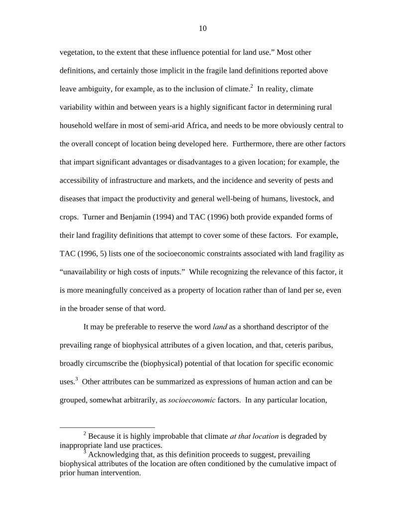
vegetation, to the extent that these influence potential for land use.” Most other

definitions, and certainly those implicit in the fragile land definitions reported above

leave ambiguity, for example, as to the inclusion of climate.2 In reality, climate

variability within and between years is a highly significant factor in determining rural

household welfare in most of semi-arid Africa, and needs to be more obviously central to

the overall concept of location being developed here. Furthermore, there are other factors

that impart significant advantages or disadvantages to a given location; for example, the

accessibility of infrastructure and markets, and the incidence and severity of pests and

diseases that impact the productivity and general well-being of humans, livestock, and

crops. Turner and Benjamin (1994) and TAC (1996) both provide expanded forms of

their land fragility definitions that attempt to cover some of these factors. For example,

TAC (1996, 5) lists one of the socioeconomic constraints associated with land fragility as

“unavailability or high costs of inputs.” While recognizing the relevance of this factor, it

is more meaningfully conceived as a property of location rather than of land per se, even

in the broader sense of that word.

It may be preferable to reserve the word land as a shorthand descriptor of the

prevailing range of biophysical attributes of a given location, and that, ceteris paribus,

broadly circumscribe the (biophysical) potential of that location for specific economic

uses.3 Other attributes can be summarized as expressions of human action and can be

grouped, somewhat arbitrarily, as socioeconomic factors. In any particular location,

2 Because it is highly improbable that climate at that location is degraded by

inappropriate land use practices.3 Acknowledging that, as this definition proceeds to suggest, prevailing

biophysical attributes of the location are often conditioned by the cumulative impact ofprior human intervention.

11

biophysical, and socioeconomic factors interact in ways that can alter the inherent

physical production potential of the land. Our primary concern here is with locations at

which human welfare and its supporting natural resource base may be at risk; whether

that be primarily as a consequence of biophysical or socioeconomic factors.

Opportunities for mitigating natural resource degradation. The land fragility literature

appears to take land as variable and land uses as fixed. Thus, the possibility that

“common practices” or “inappropriate human intervention” could evolve so as to reduce,

and perhaps even negate, resource degradation is missing from many definitions. In

reality, it is precisely this ameliorating outcome that most development strategies are

designed to bring about. There are three primary, and often simultaneous, sources of

mitigation:

• Induced Innovation—the local adaptation, experimentation, and

technological innovation by individuals, communities, and societies as a

response to external and internal pressures, e.g., the processes of induced

innovation hypothesized by Boserup (1965 and 1981), primarily as a

response to population growth.

• Formal scientific research and development (R&D)—that identifies new

policies, practices and technologies, and that has been highly successful to

date in improving agricultural productivity. With increasing concerns

about the rate of consumption of natural resources, a significant share of

public R&D investments is now being targeted to the development of so-

called “win-win” technologies that seek both to improve productivity and

12

to reduce pressure on the natural resource base. However, we must recognize

that in many instances there are tradeoffs involved.

• Market integration—integrating previously isolated communities into

regional and broader markets brings net economic benefits by stimulating the

generation of marketable surpluses using higher input production systems. In

addition to increasing income, market integration usually brings other forms

of institutional support, and a set of conditions is brought about that tend, over

time, to be land enhancing.4

Based on these considerations we conclude that the generally accepted concept of

land fragility is of limited use in a development policy context. From a development

perspective we prefer, and recommend, a spatial framework based on a broader consideration

of location rather than land wherein:

The capacity of a location to support a specific economic activity5 depends on both

biophysical factors such as climate, terrain, soil, hydrology, land cover, fauna, as well as

socioeconomic factors such as demography, income and technology constraints, physical and

institutional infrastructure, and market integration. It is recognized that the nature of the

activity, as well as human-induced and natural changes in these location-related factors, can

bring about positive or negative changes in the location’s capacity to support this (or an

alternative) activity over time.

This seems a more meaningful framework for designing strategies that foster human-

induced improvement. It does not exclude the possibility that short-term degradation could

be an optimum land management strategy (e.g., as found in fallow-based rotations), nor that

degradation can occur on “non-fragile” land if it is cultivated excessively (e.g., the

4 Although some would argue that the absence of markets for many environmental

goods and services leads to aggregate over-exploitation of land for the production of“economic” goods and services.

5 or development strategy.

13

Argentinian Pampas, or Machakos or the U.S. Dust Bowl in the 1930s), nor that degraded

lands can be rehabilitated (e.g., Machakos or the U.S. “Dust Bowl” in the 1990s).

Furthermore, it embraces the notion that, for example, markets and other institutions, and not

just technologies, can all play a role in influencing the extent to which land is degraded or

conserved.6

Location and Time

Another key issue is the temporal nature of the pressures bringing about change in

resources conditions. There are chronic pressures including: climate change and population

growth (and consequent changes in livestock and crop production), along with improvements

in infrastructure and technology, and other short-term or episodic pressures such as:

droughts, floods, disease epidemics, and pest outbreaks. From a development perspective it

is useful to separate these as requiring different, though possibly complementary, strategic

responses. Long-term pressures may best be addressed through policies related to structural

and incentive issues, while short-term pressures require some capacity for crisis response and

relief. One of the important policy challenges is to better integrate interventions, particularly

in the Sahelian countries, where short-term climatic uncertainty and extremes need to be

addressed as the long-term issues they clearly are.

Many of the concepts discussed in the previous sections are synthesized in Figure 2.

The figure highlights the complexity of land-use decisions in much of Sub-Saharan Africa,

where a range of dynamic pressures (both short- and long-term), and limited capital and other

6 While there is no shortage of concepts and empirical work on the economics of land

and location, from the works of von Thunen (1842) to those of Krugman (1998), there ismuch to be done to wed this body of work to broader development issues of the type we areaddressing.

14

Figure 2 Location specific development dynamics in sub-Saharan Africa

CollectiveDecisions Selected Land Use/Management Options

Chronic Pressures

Production& NRM

Practices

Endemic Pests & DiseasesRelated to Biophysical &Location Characteristics

Crops Livestock Human Population

PopulationGrowth

Episodic Pressures

Climatic Extremes

Rainfall, temp.

Epidemics/Outbreaks ofPests & Diseases Related to

Biophysical & LocationCharacteristics


Food & Settlement Needs

SettlementsWater, Fuel, Timber,

Fibre.

ExpectedOutputs

ActualProductivity

& NaturalResourceImpacts

HouseholdDecisions

Investment Land use Technology & input mix

Otherinfo*

Nutrition & HealthStresses


Droughts and Floods

* see Figure 1 for further details

Ag. ProductionCrops (rainfed, irrigated)Livestock (grazing, feed)Fisheries (inland, marine)Tree products

Human-Induced NaturalResource Impacts

Soil

Water

Forest, Range, Fisheries ...

SalinityDepth

Quantity

Quality

Quantity

Quality

TechnologyLabour

Purchased inputs

Natural ResourceConditions

Infrastructure DevelopmntComercializationTechnical Change

Climatic Trends &Variability

Temp.Rainfall

Market Instability Structural Adjustment, High Inflation, Devaluation, etc

15

inputs, result in high production variability and significant risk of natural resource

degradation.

GENERIC CHARACTERIZATION: PROBLEMATIC, RESTRICTIVE ANDUNNECESSARY

We have established that the scope of spatial interest, from a strategic perspective,

is location, and that location comprises both biophysical (e.g., land, broadly defined) and

socioeconomic factors. This begs the question of the feasibility of devising a practical,

generic schema for those biophysical and socioeconomic factors that might guide the

design of development strategies targeted to poverty alleviation and improved natural

resource management in Sub-Saharan Africa.

The design of any characterization schema should be based on several key

principles, including clear objectives of use, relevance to a known set of problems, and

reliance on a feasibly measurable and manageable set of characterizing variables. Even

these, seemingly trivial, requirements provide sufficient grounds to believe that a generic

schema would be impractical. For example, since poverty is a key concern we might

want to include the incidence (and, likely, severity) of poverty in any geographic area as

a key characterization variable. First, we must define a poverty metric, for which we will

need to obtain data of sufficient time and space resolution. Shall that metric be average

per-capita income, or household income—in total or by gender, or something else? And

to what extent would this metric capture other important poverty dimensions such as

health and nutritional status, and access to land, credit, and education? Even having

settled on a set of indicators, the generic, somehow-critical values of those poverty

16

indicators need to be defined.7 Natural resource issues are no less complex, including

soil erosion and soil fertility loss, water resource problems associated with over-

extraction, pollution and insecure access, the loss of genetic biodiversity, depletion of

fuelwood resources, and the growing complexity of pest and disease management.

One strategy is to aggregate characterization variables in an effort to devise a

pragmatic characterization schema, for example, to move away from direct measures of

soil organic matter, through indices of soil fertility, to soil classification. However, each

aggregation loses specificity that may, in truth, best describe the binding constraints to

development; unstable soil structure, failing property right arrangements, endemic

whitefly, fecal pollution of drinking water sources, or a host of other factors for which we

possibly have, or could assemble, data, or could make reasonable proximate estimates.

Such important details could “fall through the cracks” of a generic characterization

schema that would need to trade-off breadth (coverage) for depth (precision). Until the

scale and objectives of each development initiative are known, and until the critical

development constraints are diagnosed, we have little notion of the most relevant

variables, nor of the critical ranges of those variables, that may prove central to the

design of relevant and feasible interventions. Conversely, we maintain that

predetermined (i.e., preselected and preaggregated) generic schema are likely to impose

unnecessary restrictions of analytical scope and geographic scale.

Why may a generic schema be unnecessary? Because, without wishing to

minimize the real challenges of developing even a modest spatial analysis (GIS) capacity,

7 For a contemporary review how the spatial dimensions of human welfare and

poverty have been, and could be handled see Henninger (1998).

17

the techniques of building problem-specific characterizations in a dynamic and cost-

effective way are now little more complex, and little more expensive, than using other

large Windows-based software packages.8 Some types of data problem are also reducing

as high-resolution remote sensing data (e.g., USGS 1996), international compilations of

data (e.g., WRI 1995), and helpful analytical tools (e.g., Corbett and O’Brien 1997) are

beginning to provide solid, low-cost, start-up information on biophysical (and to a lesser

extent, socioeconomic) factors at the national level. Within most countries, other

publicly available datasets can add more spatial detail, as well as a wider range of

thematic variables, in a cost-effective manner.

Our council, then, is not to allocate scarce resources in attempting to devise a

generic classification schema, that may never properly fit any real-world problem.

Rather, we propose that the goal should be to foster the development of human, physical,

and information resources to build problem-specific characterizations as an integral part

of the strategy formulation process. The iterative nature of that process, in and of itself,

would also best be served by a capacity to quickly re-characterize and test the spatial

implications of alternative interventions. As the scope of geographic or other issues

surrounding each development problem and each intervention become better understood,

more refined characterization can be made. In this way, problem-oriented spatial

characterizations can be developed that, over time, improve the knowledge and data bases

for creating new problem-specific schema. In all cases the two dimensions of

characterization are:

• Characterization of development strategies—identifying the locational and

8 Bearing in mind that we are proposing spatial analysis capacities built around

secondary data collected and pre-processed by specialized agencies.

18

other attributes that would contribute to the success or failure of a specific

strategy. This is an essential step in identifying spatial domains within

which a given strategy is more likely to be successful.

• Characterization of locations—structuring the key spatial attributes of

land, infrastructure, demographics, poverty etc. This is important for such

tasks as problem identification, development strategy evaluation, and

technology transfer, and provides a basis for mapping locations based on

their similarity or dissimilarity. 9

By matching development strategies with locations, the improved ability to

diagnose problems and evaluate strategies, should make it possible to design

interventions that are both more effective and less costly to implement.

SPATIAL ANALYSIS TECHNIQUES

There are many potential applications of spatial analysis in the process of

designing development strategies. In the next section we will focus on just three strategy

formulation activities and, for each, illustrate a single analysis technique that is relatively

straightforward to describe and implement. However, to lay some groundwork for the

description of those applications, we will first make a brief review of the most common

spatial analysis techniques. While GIS technologies may differ in the way they represent

spatial objects and their associated properties, practically all GIS technologies support the

following:

9 When location characterization is performed only to assess the suitability of a

specific development strategy (e.g., locations are characterized using only thedevelopment strategy characterization variables) then these components are perfectlycomplementary.

19

Visualization

The mere visualization of information in its proper spatial context can foster an

understanding of some types of problems and opportunities. At the lowest level is the

presentation of different indicators using a single, fixed spatial configuration, e.g., using

district boundaries as a basis for displaying district-level statistics of population density,

crop production, average yield, head of livestock, and so on. At another level, different

types of map elements, with different boundary configurations can be precisely overlaid

for on-screen presentation or printing. This enables population density, road networks,

rainfall isohyets, soils, and other factors to be superimposed and visually examined in a

search for spatial patterns or anomalies.

Intersection

Beyond simple visual overlay of map elements, intersection supports the

analytical combination of digital maps to generate a new set of spatial (map) units as well

as cross-tabulations that summarize the spatial correspondence between values shown on

the original maps. For example, a watershed map depicting three elevation ranges, when

intersected with a population density map depicting four population density ranges, will

create a cross-table of area extents, and a corresponding spatial distribution map, of

twelve elevation-by-population density classes.

Spatial Characterization

Inductive – To identify locations having a desirable set of characteristics, relevant

characterization themes and key threshold criteria are first specified. A spatial search is

then performed across an appropriate GIS database to identify all locations satisfying the

20

specified criteria, e.g., show all areas with population density less than 50 persons per

square kilometer, river valley soils, annual rainfall of less than 500 millimeters, and

elevation ranges from 500 to 800 meters. Deductive – Here a specific location is

identified and the value ranges of variables from that location are abstracted from a user-

specified set of related maps, e.g., for a selected watershed, extract the representative

ranges of elevation, rainfall, population density, slope, and land cover that are

encountered within that watershed. Wood and Pardey (1998) provide a much more

detailed review of these methods applied to issues of agricultural research and

development, and the targeting and spillover of technology.

Distance and Network Functions

These functions allow distances between points to be calculated, as well as buffer

zones to be defined, and all objects within a certain distance to be located, e.g., find all

towns of more than 1,000 people within a radius of 50 kilometers. More sophisticated

network functions are able to recognize and manipulate points lying on the same network,

e.g., on the same road, river, and railway, and support queries such as, “find the closest

three villages by road from the current location.”

Spatial Relationships

The techniques described above take little or no account of relationships among

adjacent spatial units, but for some applications these relationships are critical.

Applications include slope determination (e.g., the relative elevation of adjacent points),

and identification of water flow pathways to the nearest river. These are relevant in

21

hydrological, soil erosion, and pollution studies. Similar algorithms support spatial

diffusion analysis, e.g., for modeling groundwater flow, or to represent diffusion of

technologies among farmers.

DEVELOPMENT STRATEGY APPLICATIONS OF SPATIAL ANALYSIS

Figure 3 presents a stylized view of the development strategy process into which a

spatial (GIS) representation of the real world has been inserted. This section will

describe how just three stages of that process could be facilitated by spatial analysis.

They are indicated on the figure by the numbers 1 to 3, and comprise: problem

diagnosis—a straightforward application of the intersection of two related themes as a

means of highlighting significant departures from an expected relationship; development

strategy characterization—a concrete example of the approach proposed in this paper - to

enable the delineation of locations appearing more or less suited to the successful

implementation of specific development strategies; and spatial extrapolation—the

characterization of locations having some desirable feature (e.g., where a specific strategy

or technology is known to have been successful) in order to find similar locations

elsewhere.

Problem Diagnosis

A classic means of establishing the well-being of an entity or process is to observe

its identifying characteristics and compare those observations against norms established

by empirical evidence or theory. The process may not provide major insight into

22

Figure 3 Spatial analysis as a component of development strategy formulation and evaluation

REAL WORLD ANALYSIS WORLD

INSTITUTIONSProblem identification and diagnosis. Defining needs and objectives, Consultation,

Intervention implementation (policies, institutions, technologies, etc)

SPATIAL WORLD

StrategyCharacterization

& Evaluation

IdentifyingIntervention

Options

Data/Knowledge

Management

Monitoring(Census

& Survey)

ProblemDiagnosis

Ad HocProblem

Area

2

1

PotentialStrategyDomains

SpatiallyTargeted

Intervention

POLICY/STRATEGY FORMULATION & EVALUATION

(search for analogous conditions (e.g., agroecology, demography, infrastructure)

SamplingNetwork

DevelopmentSuccess/Failure

3

23

causality, but it does at least identify the potential existence of a problem. Thus, if actual

crop or livestock yields, or water table levels, or fish stocks, are significantly different

from those expected, production or resource problems could be to blame. However, these

anomalies may also be due to data or method problems, issues equally worthy of

investigation. This type of comparative analysis is fairly standard even in a non-spatial

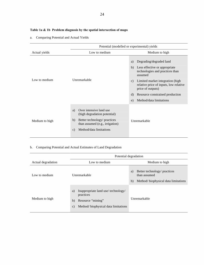
setting. Table 1 shows the format of simple cross-tabulations that a GIS could generate

by intersecting the two input maps. The table lays out the possible combinations of the

classes defined in each map, and the GIS calculates the area extent (or area proportion of

the total map area) of each combination encountered. Table 1(a) compares the area

correspondence of observed farmer yield classes (e.g., low-medium, medium-high)

against those obtained either from yield potential modeling (from a biophysical or

economic perspective) or from experimental yield data. It is essentially a spatial “yield

gap” analysis. For those combinations that warrant further investigation (high observed-

low potential, low potential-high observed) the table highlights some possible

explanations. Other combinations are considered unremarkable.

The advantage of performing this analysis in a spatial domain is that it produces

not only a table, but also a map, of the potential anomalies. This map can be visually

overlaid with other variables: rainfall, soils, and the yields of other crops to see whether

any spatial patterns emerge that help in explaining the phenomena (or in confirming data

problems). On the same basis, Table 1(b), relates potential soil degradation, (e.g.,

estimated by the USLE approach, Wischmeier and Smith 1962, or the Fertility Capability

Classification, FCC, Sanchez et al. 1982 and FAO 1997) to estimates of actual

degradation (based on empirical data or, as in the case of GLASOD, on expert

24

Table 1a & 1b Problem diagnosis by the spatial intersection of maps

a. Comparing Potential and Actual Yields

Potential (modelled or experimental) yields

Actual yields Low to medium Medium to high

Low to medium Unremarkable

a) Degrading/degraded land

b) Less effective or appropriatetechnologies and practices thanassumed

c) Limited market integration (highrelative price of inputs, low relativeprice of outputs)

d) Resource constrained production

e) Method/data limitations

Medium to high

a) Over intensive land use(high degradation potential)

b) Better technology/ practicesthan assumed (e.g., irrigation)

c) Method/data limitations

Unremarkable

b. Comparing Potential and Actual Estimates of Land Degradation

Potential degradation

Actual degradation Low to medium Medium to high

Low to medium Unremarkablea) Better technology/ practices

than assumed

b) Method/ biophysical data limitations

Medium to high

a) Inappropriate land use/ technology/practices

b) Resource “mining”

c) Method/ biophysical data limitations

Unremarkable

25

consultations with some field validation). This is an altogether more uncertain exercise

but could serve, at a minimum, to reveal any systematic biases in the potential assessment

methods, such as the improper accounting for sediment deposition when modeling soil

erosion over larger areas.

One of the significant data errors that may confound this simple type of analysis is

a mismatch in scale, or level of aggregation, between the two sources of data being

compared, and attention should be given to select or build data sets so as to minimize this

problem.

Example 1: Problem diagnosis (Yield comparison in East Africa). This example is based

on climate and yield data for Ethiopia, Kenya, and Uganda. Firstly, monthly mean

average temperature and a monthly mean aridity index10 were used to generate a map of

the potential suitability for maize production under low levels of input. Assuming that an

aridity index greater than 0.5 qualifies a month to be part of the growing season, the

Corbett and O’Brien (1997) dataset includes an estimate of the total length of growing

period (LGP) of any location. Although the Corbett and O’Brien definition of LGP is a

simplification of that used by FAO we applied the FAO’s LGP (and temperature) crop

suitability rules (Kassam et al. 1991) using the LGP and temperature variables from the

Corbett and O’Brien dataset to obtain an agroclimatic suitability map for low input,

rainfed maize production. Suitabilities were assigned to one of five levels; S1—very

suitable, S2—suitable, S3—moderately suitable, S4—marginally suitable, and N—not

10 Aridity index is the ratio of monthly rainfall to monthly potential

evapotranspiration. The climate surfaces underlying these measures were calculated byCorbett and O’Brien (1997) and are available as digital images with a spatial resolutionof 3 arc minutes.

26

suitable. The S1-S4 levels represent quartiles of the potential (biophysical) yield, i.e., S1

represents an expectation that 75-100 percent of the maximum yield could be attained at

that location. The results of this analysis are shown in Figure 4(a). With regard to actual

yield, data were generated by a joint Intergovernmental Authority on Drought and

Development (IGADD) and FAO study (van Velthuizen and Verelst 1995), in which

some 1,220 crop production system zones were delineated throughout the IGADD

countries: Sudan, Eritrea, Ethiopia, Djibouti, Somalia, Kenya, and Uganda. For each

zone a wide range of production related variables were measured and estimated,

including maize yield (see Figure 4(b)). The yield data correspond to the period 1987-90,

although the exact period varies by country. The two separate images were reduced to

just three classes, high-to-medium, medium-to-low, and not grown (actual map) or not

suitable (potential map). These maps were then intersected to produce the map shown in

Figure 4(c) and Table 2. For about 61 percent of the area there is correspondence in

terms of classification group of the two input maps. However, a significant proportion of

the area, 12.9 percent, is judged to be highly suitable, yet no actual yield is reported–

while about 5 percent of the area is considered “unsuitable” and yet produces maize in

the high yield class. The map clearly shows the large tracts where these differences occur

and Table 1 provided some suggestions as to how these differences could be interpreted

and further investigated. In this specific case the omission of soil constraints results in an

over-optimistic assessment of agricultural potential. Taking soils into account (a general,

but spatially variable, limitation) there would likely be a significant reduction of the 31.6

(0.5 + 12.9 + 18.2) percent of area in which potential yield levels appear to be overstated

relative to actual yields.

28

Table 2 Agricultural potential rating versus actual yield—maize (Ethiopia, Kenya, Uganda)

Agricultural potential ratinga

None Low-medium Medium-highActual yield

Area Share Area Share Area Share

1,000 km2 % 1,000 km2 % 1,000 km2 %

Noneb 721.6 43.6 9.0 0.5 212.6 12.9

Low-medium 131.8 7.0 18.2 1.1 181.5 18.2

Medium-high 81.1 4.9 31.9 1.9 265.4 16.1

a Based only on agroclimatic suitability—ratings would be downgraded after allowance for soil conditions.b No production in these areas.

Development Strategy Characterization and Evaluation

This technique can be used to address several related questions: How suited

would a specific development strategy be for a given set of locations (including an entire

country)? Which of the identified development strategy options would be most suited to

a given location? What mix of development strategy options would be needed to achieve

a particular goal, and how would they be targeted to match the most suited strategies to

the most appropriate locations?

In the ex ante sense used here, strategy evaluation is an iterative, two-stage

process.11 In the first stage, problem diagnosis together with a broader understanding of

the current and likely macro context, identifies some preliminary intervention

possibilities. In the second stage, these possibilities are evaluated in desk and field

studies, the outcome of which often calls for further refinement of promising strategy

11 And one that should be properly linked to the problem diagnosis and

stakeholder consultation mechanisms depicted in Figure 3.

29

options. This process is repeated until options that appear most attractive to stakeholders,

and feasible and cost-effective from an implementation standpoint, have been identified.

Our concern here is with the potential role of spatial analysis in this evaluation

process, and one possibility is to provide analysts and stakeholders with a visual and

statistical view of the geographic scope, and a qualitative feel for the intensity, of the

impact of a given strategy option. Table 3 presents a structure for characterizing strategy

options by identifying conditions that would significantly promote or hinder the

implementation of the strategy. The characterization data in such a table is of general

utility, but some aspects, e.g., development strategy requirements regarding agricultural

potential and physical infrastructure, would be of particular relevance for testing the

viability of the strategy from a geographic viewpoint. By building such a table we can

identify those variables (or proxies thereof) that have significant spatial dependency, and

that can be incorporated into the spatial development strategy characterization schema.

This approach focuses the search for appropriate spatial information, and requires

analysts to be specific about variables (and appropriate value ranges of those variables)

that are most likely to influence the outcome of a proposed strategy. Table 3 suggests

that agricultural potential is an important variable conditioning development strategy

options for any geographic area. Furthermore, it is often necessary to be specific about

the nature of the potential, e.g., upland crops, cash crops, irrigated or rainfed production.

Table 4 presents a matrix of the type required (for each location or area) as a reference

source when considering the range of agricultural options that could form the basis of a

development strategy initiative. The data for such a table can be obtained by a range of

methods, from informed expert judgement through to formal modeling. It is important

30

Table 3 Example framework for characterizing development strategies

Development strategy requirements/tolerances(e.g., enabling/negating conditions)

InfrastructureDevelopmentstrategy option Agricultural

potential Institutional PhysicalDemography

ComplementaryPolicies(E, O)a

Etc.b

Low external input CassavaMaize

ResearchExtensionNGOs

Low populationdensities

High external input (intensification)

Maize ExtensionShort-term creditLand titling

Good market access Medium-highpopulation densities

Liberalized inputmarkets (E)

Commercialization (cash crops)

CoffeeCitrus

Land titlingLong-term credit

All-weather roadsPorts

Migrant and seasonallabor

New quotaagreement

Rural non-farm industry Credit RoadsEducationElectrification

Etc.

a E—essential; O—optional.b See, for example, table 5.Shaded groups of development-related variables can exhibit high levels of spatial variability.

31

Table 4 Example framework for rating (biophysical) agricultural potentiala

Production system(technology, input mix, management intensity)

CropLow input

(Subsistence)Medium level(Smallholder)

High level(Smallholder)

Commercial

CerealsMaizeMillet…….

S3b

S2S2S2

S1S2

S2n/a

LivestockRangeland/Grazing…….

S2 S2 S1 S1

PerennialsCoffee…….

N N N N

Etc.

a For a given location or specified area.b Suitability Rating: S1–very suitable; S2–suitable; S3–moderately suitable; S4–marginallysuitable; N-Unsuitable.

that the agricultural potential be assessed for specific types of land use, that is, specific

combinations of products and production systems, since there can be significant

differences between the geographic extents not only of areas most suited to the

production of, say, sorghum, coffee, and potatoes, but also between areas most amenable

to say, predominantly manual versus predominantly mechanized production regimes

(e.g., the difficulties of manual cultivation in vertic soils and of mechanization in steeply

sloping land). Such data on agricultural potential are often obtainable from

ministries of agriculture as a lot of emphasis was given to land evaluation in Sub-Saharan

Africa in the 1980s (e.g., national studies supported by FAO in Ethiopia, Kenya,

Mozambique, Botswana, and Malawi).

32

With regard to likely natural resource requirements and impacts, Table 5 presents

some ideas about the type of information that would be required in order to bring an

explicit resource dimension to development strategy characterization. The table

identifies the resource inputs that would be needed if a particular strategy were to be

adopted, as well as the potential resource threats the strategy may pose.12 As with Table

3 (to which Table 5 represents a resource-specific extension), the expectation is that

several of the important factors identified will have a spatial component, and therefore,

could become part of the spatial (location) evaluation for that specific strategy.

Table 5 Example framework for characterizing resource aspects of development strategies

Natural resources requirements/impactsDevelopmentstrategy option Resource needsa Potential resource impacts

Low external input Organic fertilizerFuelwood

Soil fertility loss (OM, N, P)Soil erosion on steeper landForest degradation

High external input(intensification)

Irrigation water SalinizationFertilizer/pesticide leaching

Commercialization(cash crop)

Irrigation water Pesticide leachingPesticide-related health problemsof farm workers

Rural non-farm industry Wastewater quality

Etc.

Note: This table represents a simple extension of table 3.a Additional to the biophysical factors considered in assessing agricultural potential (e.g.,temperature, rainfall and soil).

12 Development strategy resource requirements and potential impacts are here

considered separately from the use of resource data as a means of estimating agriculturalpotential.

33

Summarizing, when designing and evaluating agricultural development strategies,

spatial analysis can play an initial role in assessing agricultural potential (as in the first

example, in which agricultural potential was proxied by the agroclimatic suitability of

maize at low input levels). Agricultural potential and other broader development factors,

including those specific to natural resource requirements or impacts, can then be used to

characterize each development strategy. Subsequently, these strategy-specific

characterization variables and value ranges are matched against location-specific values

held in a GIS database and, by this process, a set of strategy “domain” maps can be

generated. The geographical scope of each development strategy domain may overlap

with those of other strategies, thus delineating geographic areas where a range of

strategies may be feasible. After examining these results, each strategy can be accepted,

modified, or rejected, in order to build a portfolio of strategies likely to maximize

positive outcomes for specific target groups and regions. Within the spatial domains

delineated by any selected combination of development strategies, it would be necessary

to proceed with more detailed evaluation studies user higher resolution information and

related socioeconomic fieldwork, that may well modify initial assumptions made at the

macro level.

Example 2: Development strategy characterization and evaluation (East Africa). In this

characterization example, three hypothesized development characterization variables;

agricultural potential, population density, and a potential market integration index (PMI)

are overlaid to delineate a configuration of mutually exclusive geographic domains.

These three variables (each in two broad ranges – high and low) were proposed by

34

Pender, Place and Ehui (1999) as stratification criteria for targeting a range of agricultural

development strategies considered appropriate for Ethiopia, Kenya, and Uganda. While

Pender et al.’s criteria had been tabulated (see Table 6), they had not been fully

quantified nor translated into a spatial (map) representation.

The geographic scope of the spatial dataset compiled for this example

encompasses all of Kenya and Uganda, northern Tanzania, and southern Ethiopia. The

selection of this coverage was conditioned by the desire to use a new road network

database prepared by the World Resources Institute. In keeping with Pender et al., only

two classes were defined for the agricultural potential and population density maps (i.e.,

low-medium, medium-high), but three classes were defined for the PMI map (that was

used instead of their “market access” variable). The agricultural potential map was based

only on a single agroclimatic variable—water availability—proxied by a length of

growing period variable (LGP, one of the two variables used for the agricultural potential

map developed for example 1). In this case, an LGP of six months or more was classified

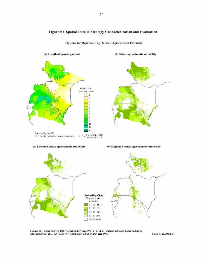
as high agricultural potential, and an LGP of five months or less as low (see Figure 5(a)).

The cut-off value was selected by visual comparison with a rainfall map since the

objective was to match the LGP variable with the 1,000mm rainfall cutoff variable

specified by Pender et al. (we preferred to use LGP as a water availability proxy since it

takes better account of seasonal rainfall distribution). It is possible, and almost certainly

desirable, to significantly improve this agricultural potential definition, both by being

more specific in terms of production systems, as well as by including additional

conditioning variables and more discriminating value ranges.

35

Table 6 Possible pathways of development in the East African Highlands

Population densityAgriculturalpotential

Marketaccess High Low

High

Central Kenya, parts of WesternKenya, Eastern Uganda

- High input cereals- Perishable cash crops- Dairy, intensive livestock- Non-perishable cash crops- Rural nonfarm development

???

HIGH

Low

Southwestern Uganda, parts ofWestern Kenya

- High input cereals- Non-perishable cash crops

Southwestern Ethiopia

- High input cereals- Non-perishable cash crops- Livestock intensification;

improved grazing areas

High

Parts of Central Tigray

With irrigation investment:- High input cereals- Perishable cash crops- Dairy, intensive livestock

Without irrigation investment:- Low input cereals- Rural nonfarm development

Parts of Northern Ethiopia

With irrigation investment:- High input cereals- Perishable cash crops- Dairy, intensive livestock

Without irrigation investment:- Low input cereals- Livestock intensification;

improved grazing areas- Woodlots- Rural nonfarm developmentL

OW

Low

Parts of Northern Ethiopia?

- Low input cereals- Limited livestock

intensification- Emigration

Much of Northern Ethiopia

- Low input cereals- Livestock intensification;

improved grazing areas

Source: Pender, Place and Ehui (1999).

Agricultural potential: High $ 1,000mm per annum, Low < 1,000m per annum rainfallPopulation density: High $ 175 persons/ha, Low < 175 persons/haMarket access: High > 100km, Low # 100km distance

36

Figures 5(b) to 5(d) illustrate crop-specific, agroclimatic suitability maps (based on an

interpretation of temperature and LGP variables). Figure 5(b) presents an aggregated

map for all maize ecotypes, while figures 5(c) and 5(d) show the sub-areas within which

lowland and highland ecotypes have high production potential.13 If commodity-specific

strategies were being evaluated, such more detailed interpretations could be substituted

for the generic agricultural potential map (5(e)) used in this example. The population

map (Deichman 1998) depicts population density for 1990 by third level administrative

unit. The map shown in Figure 5(f) was reclassified for the purposes of this analysis into

only two classes; low to medium population density (less than 175 persons per square

km.), and medium to high population density (175 or more persons per square km). This

corresponds exactly with the Pender et al. cutoff for this variable. The final variable,

PMI, is based on an algorithm reported by Deichmann (1997), and has been previously

used in the generation of regional population density maps (Tobler et al. 1995). For any

location the PMI represents an accumulated index of the travel time to the nearest n target

locations (markets), weighted by the population of each market location. “Nearest” is

assessed in terms of lowest travel time across a transport network (including off-road

travel time to reach the closest network point), and in this example the nearest three target

locations were used to build the index. Market locations were defined as gazetted

settlements having a population of greater than 5,000 inhabitants. Travel times along any

segment of the transport network depend upon travel speed, and speed is conditioned by

the nature of the surface, e.g., 60 km/h on a surfaced road, 25km/h on a dirt road,

13 And Figure 13 in the Appendix describing the use of soil information in Sub-

Saharan Africa shows a complementary interpretation of the agroedaphic suitability ofmaize.

40

and 7 km/h walking on a level path. Figure 5(g) shows the resultant map of the PMI

variable reclassified into just the three ranges used in this example; No (market

integration), low to medium, and medium to high. For the sake of clarity, only major

cities, and not all settlements used in the analysis, are shown on the map. The cutoff

value of the index between low and high was approximated visually to Pender et al.’s

criteria of 100km distance to market, but the two measures do not correspond well since

the PMI is much richer in its information content.

The intersection of the three input themes yielded a map showing 12 strategy

domains (two agricultural potential classes, by two population density classes, by three

PMI classes) as well as a cross-tabulation of the corresponding domain extents (Table 7).

The table shows that just under one third of the area examined falls in the

category L(ow)-L(ow)-L(ow) for agricultural potential, population density, and PMI

respectively, and less than three percent into the category H(igh)-H(igh)-H(igh). Of

potential development interest are areas such as H-L-H, representing 8.8 percent of the

mapped area, where there would appear to be the possibility for expanded agricultural

output (based on the in-migration of labor) with minimal infrastructure (roads)

investment, although clearly there are many omitted variables, such as the prevalence of

pests and diseases, that could help explain the apparent status quo. Data and method

constraints should always be kept in mind and certainly one major limitation in this

example is the highly aggregated (small number of) classes used for each variable. It

appears worthwhile to further explore how well the PMI variable may serve as a proxy

not only for a range of transport and other transactions costs, but also for technology

diffusion and public services.

41

Table 7 Preliminary estimation of development strategy domains (areas in square kilometers)

Low population densitya High population densitya

Low PMI Med PMI High PMI Low PMI Med PMI High PMI Low PMI Med PMI High PMI Low PMI Med PMI High PMICountry

Low agricultural potentialb High agricultural potential Low agricultural potential High agricultural potential

Ethiopia 119,736 81,115 4,394 47,224 114,203 16,154 174 87 792 174 14,049 6,585

Kenya 104,818 337,059 31,980 100 26,831 33,090 - 910 5,050 - 2,830 26,332

Tanzania 27,177 72,901 21,428 19,344 163,073 48,408 98 - 1,287 98 196 1,986

Uganda 97 17,115 - 387 120,783 44,504 - - - 97 3,421 13,598

TOTAL 251,827 508,189 57,802 67,054 424,890 142,155 272 997 7,129 368 20,496 48,501

Notes: PMI (Potential Market Integration) is an index. Ethiopia and Tanzania are only partially included (see Figure 5e).a Low population density < 175 person/km2, high population density $ 175 person/km2.b Water availability (P/ET > 0.5) in months per year. High $ 6 months, Low < 6 months.

Table 8 Preliminary estimation of total population within strategy domains (thousands)

Low population densitya High population densitya

Low PMI Med PMI High PMI Low PMI Med PMI High PMI Low PMI Med PMI High PMI Low PMI Med PMI High PMICountry

Low agricultural potential High agricultural potential Low agricultural potential High agricultural potential

Ethiopia 544 935 404 1,124 7,084 1,892 44 12 166 27 3,364 3,081

Kenya 60 2,627 1,790 22 1,156 4,181 0 87 2,069 0 482 8,162

Tanzania 95 1,796 1,604 80 5,743 4,183 126 0 335 6 6 1,234

Uganda 0 185 0 15 5,510 5,044 0 0 0 15 6,53 4,470

TOTAL 701 5,544 3,799 1,242 19,494 15,301 170 99 2,571 49 4,506 16,948

Note: PMI (Potential Market Integration) is an index. Agricultural potential: Water availability (P/ET > 0.5), Months per year, High $ 6 months, Low < 6 months.a Low population density < 175 person/km2, high population density $ 175 person/km2.

42

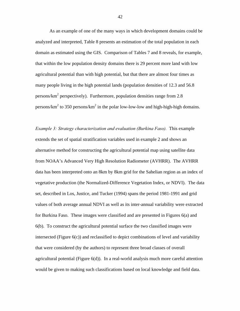
As an example of one of the many ways in which development domains could be

analyzed and interpreted, Table 8 presents an estimation of the total population in each

domain as estimated using the GIS. Comparison of Tables 7 and 8 reveals, for example,

that within the low population density domains there is 29 percent more land with low

agricultural potential than with high potential, but that there are almost four times as

many people living in the high potential lands (population densities of 12.3 and 56.8

persons/km2 perspectively). Furthermore, population densities range from 2.8

persons/km2 to 350 persons/km2 in the polar low-low-low and high-high-high domains.

Example 3: Strategy characterization and evaluation (Burkina Faso). This example

extends the set of spatial stratification variables used in example 2 and shows an

alternative method for constructing the agricultural potential map using satellite data

from NOAA’s Advanced Very High Resolution Radiometer (AVHRR). The AVHRR

data has been interpreted onto an 8km by 8km grid for the Sahelian region as an index of

vegetative production (the Normalized-Difference Vegetation Index, or NDVI). The data

set, described in Los, Justice, and Tucker (1994) spans the period 1981-1991 and grid

values of both average annual NDVI as well as its inter-annual variability were extracted

for Burkina Faso. These images were classified and are presented in Figures 6(a) and

6(b). To construct the agricultural potential surface the two classified images were

intersected (Figure 6(c)) and reclassified to depict combinations of level and variability

that were considered (by the authors) to represent three broad classes of overall

agricultural potential (Figure 6(d)). In a real-world analysis much more careful attention

would be given to making such classifications based on local knowledge and field data.

44

The final image, even though aggregated into only three classes, shows some significant

spatial variability that is not apparent from looking at long-term average precipitation or

LGP maps alone. Compared to the aridity index proxy used in example 1, the NDVI-

based agricultural potential is significantly more precise because it represents location-

specific integration of both climate and soil conditions.14 A limitation of coarse

resolution NDVI is that it is strictly a “greeness” indicator and does not differentiate

reliably between different types of vegetation, e.g., forest, grassland and cropland.

However, other global, regional and national sources of information on land cover and

land use could be used to further fine-tune the agricultural areas.

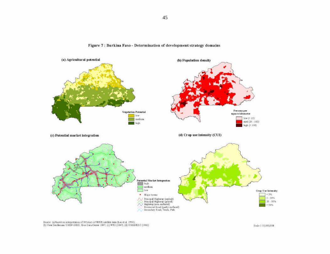
The Burkina Faso population density and PMI maps (Figures 7(b) and 7(c)) are

taken from the same sources as in example 2. The new information included in this

example is Crop Use Intensity (CUI), a measure of the percentage of land area under

cultivation. The CUI variable is based on interpretation of Landsat imagery together with

groundtruthing survey data from the early 1990s. The original dataset is classified into

five levels of CUI ranging from low, 0-5 percent area cultivated, to high, greater than 70

percent cultivated (Dalsted and Westin 1996). By intersecting the four maps of

agricultural potential, population density, PMI and CUI (Figures 7(a)-7(d) respectively)

an illustrative development strategy domain map was generated for Burkina Faso.

Two partial views of that final map are presented in Figures 8(a) and 8(b). Figure

8(a) highlights the areas having low to medium agricultural potential, but within which

14 Noting that the rainfall and potential evapotranspiration surfaces used to derive

the aridity index are based on the spatial extrapolation of point (climate station) data.The climate station network in most rural areas of Burkina Faso is likely to be very muchmore sparse than the spatial resolution of the AVHRR observations.

47

there is both significant actual cultivation and medium to high population density. In such

areas there is clearly scope for high social returns to investment that could raise the

productivity of agriculture – because agriculture is extensively practiced, and because

there are many people (both as producers and consumers). Such areas may benefit from

public investment policies that, for example, target agricultural R&D to address the

technological problems faced, and that facilitate development of input markets and small-

scale credit schemes. In areas where market integration is limited (low PMI) the existing

significant presence of both people and agriculture might suggest specific investment in

road infrastructure might be worthwhile. Clearly, there will also be a range of

institutional and micro issues that warrant attention, but these would need to be identified

through parallel assessments.

In the high agricultural potential areas (Figure 8(b)) other development issues can

be addressed. One is the extent to which high potential areas may be currently

“underutilized” (low CUI) from an agricultural perspective. There may be very good

reasons for this, such as the existence of forests, conservation areas, wildlife parks, and so

on, but this situation could also be indicative of potentially modifiable constraints to

agricultural expansion and intensification, such as endemic human and animal diseases,

regional insecurity, or severe lack of infrastructure.

In all cases, spatial stratification coupled with appropriate local knowledge and

interpretation can provide analysts and decisionmakers with relatively low-cost insights

into development constraints and opportunities, how significant they may be, and how

complex they may be to address (for example, are problems specific to a few contiguous

areas or are they fragmented across much larger areas). Table 9 presents the full

48

summary of the area extent within each domain of this protoype spatial stratification for

Burkina Faso, but other variables, and other boundary values would probably need to be

tested in a formal analysis. And, as in the previous example, the strategy domains can be

characterized in terms of, say, total population (see Table 10), area of agricultural land

(see Table 11), road density, or any other relevant indicator to support further assessment

of their value for development planning purposes.

Table 9 Total population within each preliminary development strategy domain for Burkina Faso(thousands)

LowPMI

MediumPMI

HighPMI

LowPMI

MediumPMI

HighPMI

LowPMI

MediumPMI

HighPMICrop use

intensity (CUI)Low agricultural potential Medium agricultural potential High agricultural potential

CUI in low population densityZero – 5 percent 208 368 27 78 192 14 36 120 95 - 30 percent 12 105 9 5 17 3 10 30 NA30 - 50 percent 7 50 14 9 164 31 12 156 26> 50 NA NA NA 7 3 NA NA NA NATOTAL 227 523 50 99 376 48 58 306 35

CUI in medium population densityZero – 5 percent 179 720 160 21 431 139 7 159 65 - 30 percent 36 167 35 3 188 54 3 88 030 - 50 percent 18 229 130 40 1,161 892 2 381 157> 50 2 NA NA 5 10 NA NA NA NATOTAL 235 1,351 325 69 1,790 1,085 12 628 163

CUI in high population densityZero – 5 percent 46 53 39 NA 19 23 NA 8 55 - 30 percent NA NA NA NA NA NA NA 23 3830 - 50 percent NA NA NA NA 184 1,062 NA 48 223> 50 NA NA NA NA NA NA NA NA NATOTAL 46 53 39 NA 203 1085 NA 79 266

CUI across all areasZero – 5 percent 433 1,141 226 99 642 176 43 287 205 - 30 percent 48 272 44 8 205 57 13 141 3830 - 50 percent 25 279 144 49 1,509 1,985 14 585 406> 50 2 NA NA 12 13 NA NA NA NATOTAL 508 1,692 414 168 2,369 2,218 70 1,013 464

Note: Population density is defined as: Low: < 25 person/km2; medium: 25-100 person/km2; and high > 100person/km2. PMI (Potential Market Integration) is an index. CUI (Crop Use Intensity) is a percentage of areacultivated. Agricultural potential is an index based on interpretation of NOAA’s AVHRR satellite data.

49Table 10 Total population within each preliminary development strategy domain for Burkina Faso(thousands)

LowPMI

MediumPMI

HighPMI

LowPMI

MediumPMI

HighPMI

LowPMI

MediumPMI

HighPMICrop use

intensity (CUI)Low agricultural potential Medium agricultural potential High agricultural potential

CUI in low population densityZero – 5 percent 208 368 27 78 192 14 36 120 95 - 30 percent 12 105 9 5 17 3 10 30 NA30 - 50 percent 7 50 14 9 164 31 12 156 26> 50 NA NA NA 7 3 NA NA NA NATOTAL 227 523 50 99 376 48 58 306 35

CUI in medium population densityZero – 5 percent 179 720 160 21 431 139 7 159 65 - 30 percent 36 167 35 3 188 54 3 88 030 - 50 percent 18 229 130 40 1,161 892 2 381 157> 50 2 NA NA 5 10 NA NA NA NATOTAL 235 1,351 325 69 1,790 1,085 12 628 163

CUI in high population densityZero – 5 percent 46 53 39 NA 19 23 NA 8 55 - 30 percent NA NA NA NA NA NA NA 23 3830 - 50 percent NA NA NA NA 184 1,062 NA 48 223> 50 NA NA NA NA NA NA NA NA NATOTAL 46 53 39 NA 203 1085 NA 79 266

CUI across all areasZero - 5 percent 433 1,141 226 99 642 176 43 287 205 - 30 percent 48 272 44 8 205 57 13 141 3830 - 50 percent 25 279 144 49 1,509 1,985 14 585 406> 50 2 NA NA 12 13 NA NA NA NATOTAL 508 1,692 414 168 2,369 2,218 70 1,013 464

Note: Population density is defined as: Low: < 25 person/km2; medium: 25-100 person/km2; and high > 100person/km2. PMI (Potential Market Integration) is an index. CUI (Crop Use Intensity) is a percentage of areacultivated. Agricultural potential is an index based on interpretation of NOAA’s AVHRR satellite data.

Table 11 Crop use intensity for each preliminary development strategy domain for Burkina Faso

LowPMI

MediumPMI

HighPMI

LowPMI

MediumPMI

HighPMI

LowPMI

MediumPMI

HighPMICrop Use

Intensity (CUI)Low agricultural potential Medium agricultural potential High agricultural potential

(percentage) (percentage) (percentage)

Low 1-7 3-12 9-22 2-9 9-20 15-28 3-12 12-25 20-35Medium 4-13 7-17 11-23 20-36 20-36 24-42 6-17 18-35 29-48High 0-5 0-5 0-5 0 27-45 28-47 0 20-39 26-46

TOTAL 1-8 4-14 10-22 4-12 16-30 23-41 3-12 14-29 26-44

Note: PMI (Potential Market Integration) is an index. CUI (Crop Use Intensity) is a percentage of areacultivated. Agricultural potential is an index based on interpretation of NOAA’s AVHRR satellite data.

50

Benchmark Sites and Extrapolation Domains

This is a relatively simple application in which a specific location (the benchmark

location), known to have some desirable properties is characterized, and those

characteristics are used as the basis of a GIS search to locate similar (analogous)

locations. There are many reasons why a benchmark location could have important

characteristics that warrant searching for elsewhere. In our context, the most likely

benchmark locations would be those where certain strategies have been successful, and

the hope would be that this procedure could identify other locations where such

interventions may have the same favorable outcome. The problem, common to all

characterization endeavors, is to select the most relevant and complementary set of

characterization variables. Once those variables have been identified (and presuming we

have, can obtain, or can approximate data for their spatial representation), we extract their

value ranges at the benchmark location from the GIS database. Those (user determined)

variables, and (computer determined) value ranges create the characterization schema for

the benchmark site which can then be used in a subsequent GIS operation to locate all

other similar areas within a specific geographic extent.

Example 4: Spatial extrapolation (East Africa). Using the same variables as for example

2 (agricultural potential, population density, and potential market integration - PMI) the

district of Machakos was selected as a benchmark location and the GIS was used to

determine the range of values of the three variables within that district. On the basis of

that determination, other locations (in this case third level administrative units) were

examined within the same geographical extent as example 2 (i.e., omitting southern

51

Tanzania and northern Ethiopia) in order to find like areas. The output of this search is

shown in Figure 9, and highlights the relatively unique nature of the Machakos district in

the early 90s. From a development perspective it would be most interesting to undertake

this type of analysis based on the characteristics of Machakos areas at different stages of

its documented degradation and rehabilitation, or by constructing characterization

variables that reflect the integration of human activities over time.

It should be noted that there are other, more sophisticated methods of

“automated” site characterization and extrapolation, primarily the use of cluster analysis

(see Wood and Pardey 1998), but the basic sequence of operations remains as described

above.

3. CONCLUSIONS15

The notion that spatial perspectives provide significant benefits to policy analysts and

others is based on evidence that rural development opportunities are affected by spatial

patterns and processes related to the environment, demography, and infrastructure.

Moreover, many “non-spatial” policy, market, and institutional variables exhibit spatial

aspects that can be taken into account.16

15 Some separate conclusions regarding data aspects of strategic assessment at a

regional scale are given in the appendix (section3).16 In reality, few of the measurable variables with which we are concerned are

truly “non-spatial.” Policy variables and household data, are oft quoted examples of non-spatial data. But policies, e.g., taxes, subsidies, quotas, and so on, have a spatial limit ofvalidity such as a country boundary and, at a different scale, most households can belocated spatially, even if the location changes in time (such as with transhumance).

53

Formulating good development strategies is a complex matter. One of the complexities is

the dynamic interaction among natural and human-induced factors and the stocks and

flows of natural and other resources. Obtaining an improved vision, literally and

metaphorically, of such interactions can foster improved approaches to policy

formulation, not only by the existence of a geographically referenced universe, but also

because geographical information systems (GIS) support the analytical integration of

spatial and (seemingly) non-spatial data. The spatial framework can be catalytic by

providing both a common focus for multidiscipline inputs to designing and testing

development strategies, as well as common formats for the integration of multi-discipline

information. This framework presents opportunities for time and cost savings in design

and analysis, and offers considerable scope for shaping more effective strategy options.

This is particularly so if a spatial structure can serve to make the policy process more

understandable to non-specialists and, by this means, make the process more accessible to

a greater range of stakeholders. With these considerations in mind we have proposed

bringing an explicit spatial dimension to the procedures by which problems are identified

and diagnosed, strategies designed and tested, and knowledge is extrapolated from local

experience.

With regard to the specific challenge of developing a characterization schema for

the fragile lands of Sub-Saharan Africa in the context of designing improved

development strategies, we have expressed several reservations. Firstly, the term “fragile

lands,” and its various definitions, appear inadequate to capture the broad range of

development issues that underlie the concern for its characterization. We interpret that

significant concern to be the search for development strategies (policy instruments,

54

institutions, and technologies) that contribute to conserving, and perhaps improving, the

long-term productive capacity of natural resources while satisfying the needs of current

populations. From this development policy perspective we have suggested that “the

suitability of a location to support specific economic activities over time” rather than land

fragility would be a more appropriate focus. We consider that human-induced changes in

suitability are brought about by the cumulative impact of a host of biophysical and

socioeconomic factors, the scope and relative importance of which depends upon the

precise nature of the economic activities (in our case, agricultural production activities)

involved. We, thus, conclude that a generic characterization schema would be extremely

difficult to conceive, limited in its practical value and, perhaps above all, unnecessary.

Rather we recommend investment in programs and methods that foster the build-up of

human and technical capacity to generate problem-specific characterization schema that

are certain to change as our databases, analytical tools, and fundamental understanding of

development processes and outcomes improve.

The basic contention of this paper has been that developing the capacity to

acquire, generate, manage and interpret spatial information, and using it creatively in the

strategy development process would focus, accelerate, and enrich that process, and

ultimately improve the likelihood of favorable social and environmental outcomes. The

paper sets out some ambitious, but achievable, ideas about how methods not traditionally

embraced by economists (who are normally among the closest to the policy process)

could be used to support and improve strategy design and development. The visual

presentation of data in spatial formats, in and of itself, can bring a new perspective on

agricultural and resource-related issues. An overview of the relative spatial distribution

55

of key variables may offer some insights into causality, as well as point to issues of data

resolution and quality. Most importantly, the approach offers a geographically-focused

perspective of the likely feasibility and attractiveness of specific development options in

agriculture - an activity whose success is often critically dependent on location-specific

factors.

56

REFERENCES

Aubert, G., and P. Duchaufour. 1956. Projet de classification des sols. In Rapports, VIecongrès international de la science du sol. Paris.

Batjes, N.H., et al. 1997. Soil data derived from WISE for use in global and regionalAEZ studies (version 1.00). <http://iiasa.ac.at>.

Boserup, E. 1965. The conditions of agricultural growth: The economics of agrarianchange under population pressure. London: Allen and Unwin.

Boserup, E. 1981. Population and technological change: A study of long-term trends.Chicago, Il.: The University of Chicago Press.

Braun, A.R., et al. 1997. Maintenance and improvement of soil productivity in thehighlands of Ethiopia, Kenya, Madagascar and Uganda: An inventory of spatialand non-spatial survey and research data on natural resources and landproductivity. AHI Technical Report Series No. 6. Kenya: Africa HighlandInitiative.

Brunner, J., and D. Nielsen. 1997. Land use stratification for natural resourcemanagement monitoring in the Sahel. WRI (World Resources Institute),Washington, D.C.

CCD (Convention to Combat Desertification). 1995. United Nations convention tocombat desertification in those countries experiencing serious drought and/ordesertification, particularly in Africa – Text with Annexes. No. CCD/95/1.Geneva, Switzerland: UNEP (United Nations Environment Programme).

Corbett, J.D., and R.F. O’Brien. 1997. The spatial characterization tool. TexasAgricultural Experimentation Station, Texas A&M University System. CD-ROM.

Crosson, P. 1995. Soil erosion estimates and costs. Science 269: 461-63.

Crosson, P., and J.R. Anderson. 1995. Achieving a sustainable agricultural system inSub-Saharan Africa. Building blocks for environmentally sustainabledevelopment in Africa No. 2. Washington, D.C.: The World Bank.

Dai, A., Y. Fung, and D. del Genio. 1997. Surface observed global land precipitationvariation during 1900-1988. Journal of Climate 10: 2943-62.

Dai, A., K.E. Trenberth, and T.R. Karl. 1998. Global variations in droughts and floods:1900-1995. Submitted to Geophysical Resource Literature. Mimeo.

Dalsted K., and F. Westin. 1996. An overview and evaluation of cropland use intensityin Africa. Report under USGS Contract 1434-92-C-4004.

57

Deichmann, U. 1997. Accessibility indicators in GIS. New York: United NationsStatistics Division.

Deichmann, U. 1998. A review of spatial population database design and modeling.Santa Barbara: University of California, National Center for GeographicInformation and Analysis.

FAO (Food and Agriculture Organization of the United Nations). 1971. FAO/UNESCOsoil map of the world. 10 Volumes, 19 Map Sheets. Paris: UNESCO (UnitedNations Education and Science Organization).

FAO (Food and Agriculture Organization of the United Nations). 1976. A framework forland evaluation. FAO Soils Bulletin No. 32. Rome.

FAO (Food and Agriculture Organization of the United Nations). 1978. Report on theagro-ecological zones projects, Vol. 1: Methodology and results for Africa.World Soil Resources Report No. 48. Rome.

FAO (Food and Agriculture Organization of the United Nations). 1991. A study of thereasons for success or failure of soil conservation project. Soils Bulletin No. 63.Rome.

FAO (Food and Agriculture Organization of the United Nations), et al. 1993. Globaland national soils and terrain digital databases (SOTER). World Soil ResourcesReport No. 74. Rome.

FAO (Food and Agriculture Organization of the United Nations). 1995. The digital soilmap of the world and derived soil properties. (Version 3.5). CD-ROM. Rome.

FAO (Food and Agriculture Organization of the United Nations). 1996. Land husbandry– components and strategy. Soils Bulletin No. 70. Rome.

FAO (Food and Agriculture Organization of the United Nations). 1997. Agro-ecologicalzoning guidelines. Soils Bulletin No. 73. Rome.

FAO (Food and Agriculture Organization of the United Nations). 1997. The digital soiland terrain database of East Africa (SEA). Mimeo.

FAO (Food and Agriculture Organization of the United Nations), University of Hawaii,and USDA (United States Department of Agriculture) Natural ResourceConservation Service. 1997. Merging databases and decision-aids: Linking anupdated soil fertility capability classification (FCC3) with the WISE (Worldinventory of soil emission potentials) database. Final Project Report. Honolulu,Hawaii.

FAO (Food and Agriculture Organization of the United Nations). 1998. World overviewof conservation approaches and technologies (WOCAT). CD-ROM. Rome.

58

FAO (Food and Agriculture Organization of the United Nations), ISRIC (InternationalSoil Resources Information Center), and ISSS (International Soil SciencesSociety). 1998. World reference base for soil resources. World Soil ResourcesReport No. 84. Rome.

FAO (Food and Agriculture Organization of the United Nations). 1998. Soils of EastAfrica and crop production zones of IGADD countries. Land and Water DigitalMedia Series No. 2. Rome.

FAO (Food and Agriculture Organization of the United Nations). 1998. Land coverclassification system: Classification concepts and user manual. CD-ROM.Rome.

FAO (Food and Agricultural Organization of the United Nations). 1998. FCC3 –Diagnosing constraints to crop growth with a decision aid linked to a soildatabase.<http://ftp.fao.org/WAICENT/FaoInfo/Agricult/AGL/AGLS/fcc3.HTM>(accessed 1998).

Fischer, G.W., et al. 1996. A provisional world climate resource inventory based on thelength of growing period concept. In Proceedings of the NASREC Workshop 5-12November, 1995. ISRIC (International Soils Resources Information Center):Wageningen, The Netherlands.

Fisher, G., et al. 1996. The potential effects of climate change on world food productionand security. Chapter 9 in Global climate change and agricultural production,ed. F. Bazzaz and W. Sombroek, 199-236. London: John Wiley & Sons.

Fontaine, B., and S. Janicot. 1996. Sea surface temperature fields associated with WestAfrican rainfall anomaly types. Journal of Climate 9: 2935-40.

Hansen, J., and S. Lebedeff. 1987. Global trends of measured surface air temperature.Journal of Geophysical Research 92 (13): 345-72.

Hassan, A. 1996. Improved traditional planting pits in the Tahoua Department, Niger.In Sustaining the soil: Indigenous soil and water conservation in Africa, ed. C.Reij, I. Scoones, and C. Toulmin. London: Earthscan Publishers Limited.

Henninger, N. 1998. Mapping and geographic analysis of human welfare and poverty –review and assessment. WRI (World Resources Institute). Mimeo.

Houghton, J.T. 1997. Global Warming. Cambridge: Cambridge University Press.

IBRD (International Bank for Reconstruction and Development). 1989. InternalEvaluation Report. Washington, D.C.

IGBP (International Geosphere and Biosphere Program) and DIS (Data InformationSystem). 1998. The IGBP-DIS global 1 km land cover data Set “Discover” –

59

proposal and implementation plans. IGBP-DIS Working Paper No. 13.Toulouse.

IPCC (International Panel on Climate Change). 1990. Climate change, IPCC scientificassessment. ed. J.T. Houghton, G.J. Jenkins, and J.J. Ephraums. Cambridge:WMO (World Meteorological Organization) and UNEP (United NationsEnvironment Programme), Cambridge University Press.

IPCC (International Panel on Climate Change). 1996. Climate change 1995.Contribution of WGI to the second assessment of report to the intergovernmentalpanel on climate change, ed. J.T. Houghton et al. Cambridge: CambridgeUniversity Press.

Kassam, A.H., et al. 1991. Agro-ecological land resources assessment for agriculturaldevelopment planning: A case study of Kenya resources database and landproductivity. Technical Annex 4 – Crop Productivity. World Soil ResourcesReports No. 71/4. FAO (Food and Agriculture Organization) Land and WaterDevelopment Division, and International Institute for Applied Systems Analysis.

Koohafkan, P., F. Nachtergaele, and J. Antoine. 1997. Use of agro-ecological zones andresource management domains for sustainable management of Africa wetlands.Paper presented at the Wetland Conference, Harare, Zimbabwe.

Krugman, P. 1998. Space: The final frontier. The Journal of Economic Perspectives 12(2): 161-74.

Kruska, R.L., B.D. Perry, and R.S. Reid. 1995. Recent progress in the development ofdecision support systems for improved animal health. In Proceedings of theAfrica GIS ‘95 meeting, integrated geographic information systems useful for asustainable management of natural resources in Africa. Abidjan.

Lamb, P.J., and A. Peppler. 1991. West Africa. In Teleconnections linking worldwideclimate anomalies, ed. M. Glantz, R.W. Katz, and N. Nicholls, 121-89.Cambridge: Cambridge University Press.

Lamb, P.J., and A. Peppler. 1992. Further case studies of tropical Atlantic surfaceatmospheric and oceanic patterns associated with sub-Saharan drought. Journalof Climate 5: 476-88.

Lamb, P.J., and A. Peppler. 1995. The science of climate change. In Contribution ofWGI to the second assessment of report of the intergovernmental panel on climatechange, ed. J.T. Houghton et al. Cambridge: Cambridge University Press.

Los, S.O., C.O. Justice, and C.J. Tucker. 1994. A global 1 by 1 NDVI dataset forclimate studies derived from the GIMMS continental NDVI data. InternationalJournal of Remote Sensing 15 (17): 3493-518.

60

MacVicar, C.N., et al. 1977. Soil classification, a binomial system for South Africa.Department of Agricultural Technical Services: Pretoria, South Africa.

Nachtergaele, F. 1996. From the soil map of the world to the global soil and terraindatabase: 1960-2000. AGLA (Soil Resources Management and ConservationService), Working Paper.

Nachtergaele, F., and R.B. Brinkman. 1996. Identification of analogous land foragrotechnology transfer in the Savannah zones of the developing world.Integrated Crop Management Series 1: 29-41.

Nicholson, S.E. 1989. African drought: Characteristics, casual theories and globalteleconnections. In Understanding climate change, ed. A. Berger, R.E.Dickinson, and J. Kidson, 79-100. Washington, D.C.: American GeophysicalUnion.

Nicholson, S.E. 1993. An overview of African rainfall fluctuations of the last decade.Journal of Climate 6: 1463-66.

Nicholson, S.E., and J. Kim. 1997. The relationship of the El Niño-southern oscillationto African rainfall. International Journal of Climatology 17: 117-35.

Oldeman, L.R., R.T.A. Hakkeling, and W.G. Sombroek. 1990. World map of the statusof human-induced soil degradation: An explanatory note. Global assessment ofsoil degradation (GLASOD). Nairobi: International Soil Reference andInformation Center and United Nations Environment Programme.

Oldeman, L.R., R.T.A. Hakkeling, and W.G. Sombroek. 1991. World map of the statusof human-induced soil degradation. Nairobi: United Nations EnvironmentProgramme.

Pardey, P.G., and S. Wood. 1994. Targeting research by agricultural environments.Chapter 31 in Agricultural technology: policy issues for the internationalcommunity, ed. J.R. Anderson, 566-89. Oxon, U.K.: CAB International.

Pender, J., F. Place, and S. Ehui. 1999. Strategies for sustainable agriculturaldevelopment in the East African highlands. Environment and ProductionTechnology Division Discussion Paper No. 41. International Food PolicyResearch Institute, Washington, D.C.

Pimentel, D., et al. 1976. Environmental and economic costs of soil erosion andconservation benefits. Science 194 (149).

Reij, C., I. Scoones, and C. Toulmin. 1996. Sustaining the soil: Indigenous soil andwater conservation in Africa. London: Earthscan Publishers Limited.

61

SADC (Southern African Development Council). 1997. The database of SADC: Theregional remote sensing project (RRSP). CD-ROM. Harare, Zimbabwe.

Sanchez, P.A., W. Couto, and S. Buol. 1982. The fertility capability classificationsystem: interpretation, applicability and modification. Geoderma 27: 283-309.

Scherr, S. J., G. Bergeron, J. Pender, and B. Barbier. 1996. Policies for sustainabledevelopment in fragile lands: Methodology overview. Fragile Lands Program.Environment and Production Technology Division. International Food PolicyResearch Institute, Washington, D.C. Mimeo.

Shea, D.J. 1986. Climatological atlas: 1950-1979. NCAR Technical Note No. TN-269+STR. Boulder, Colo.: National Center for Atmospheric Research.

Smaling, E. 1993. An agro-ecological framework for integrated nutrient managementwith special reference to Kenya. Ph.D., Wageningen University, TheNetherlands.

Soil Survey Staff. 1994. Keys to soil taxonomy. Sixth ed. Washington, D.C.: USDA(United States Department of Agriculture) Soil Conservation Service.

Stocking, M. 1986. The cost of soil erosion in Zimbabwe in terms of the loss of threemajor nutrients. Rome: FAO (Food and Agriculture Organization) SoilResources Management and Conservation Program.

TAC (Technical Advisory Committee) Secretariat and FAO (Food and AgricultureOrganization of the United Nations). 1996. Report of the study on CGIARresearch priorities for marginal land: Agenda item 3. Report presented at theSeventy-First Meeting of the International Livestock Research Institute, AddisAbaba, Ethiopia.

Tiffen, M., M. Mortimore, and F. Gichuki. 1994. More people—less erosion:Environmental recovery in Kenya. London: John Wiley & Sons.

Tobler, W., et al. 1995. The global demography project. Technical Report No. TR 95-6.Santa Barbara: University of California, Santa Barbara.

Trenberth, K.E., and T.J. Hoar. 1997. El niño and climate change. GeophysicalResource Literature 24: 3057-60.

Turner II, B.L., and P.A. Benjamin. 1994. Fragile lands: Identification and use foragriculture. Chapter 5 in Agricultural environment and health: Sustainabledevelopment in the 21st century, ed. V. Ruttan, 104-45. Minnesota: University ofMinnesota Press.

UNSO (United Nations Sahelian Office). 1997 An assessment of population levels in theworld's drylands: Aridity zones and dryland populations. New York: UNSO andUNDP (United Nations Development Programme).

62

USGS (United States Geological Survey). 1996 Digital elevation model for Africa 1 kmby 1 km. <http://edcwww.cr.usgs.gov/landaac/glcc/glcc.html> (accessed 1998).

Van Velthuizen, H., and L. Verelst. 1995. Crop production system zones of the IGADDsub-region. Agrometeorology Working Paper Series No. 10. Rome: IGADD(Intergovernmental Authority on Drought and Development) and FAO (Food andAgriculture Organization).

Von Thunen, J.H. 1842. Der Isolierte Staat. In Von Thunen’s isolated state, ed. P. Hall.London: Pergamon.

Wint, W., and D. Rogers. 1998. Predictions of cattle density, cultivation levels andfarming systems in Kenya. Consultants’ Report. Rome: FAO - AGA (Food andAgriculture Organization, Animal Production Division).

Wischmeier, W.H., and D.D. Smith. 1962. Soil loss estimation as a tool in soil andwater management planning. International Association of Scientific HydrologyPublication 59: 148-59.

Wood, S., and P.G. Pardey. 1998. Agroecological aspects of evaluating agriculturalR&D. Agricultural Systems 57 (1): 13-41.

World Bank. 1996. Natural resources management. Findings. Africa Region, No. 8,September.

WRI (World Resources Institute). 1995. Africa data sampler. CD-ROM. WashingtonD.C.

63

APPENDIX: A REGIONAL OVERVIEW OF CLIMATE, SOIL, AND TERRAINCONDITIONS AND DATASETS FOR SUB-SAHARAN AFRICA

Section one identified climate, soil, and terrain as key biophysical determinantsthat condition both the suitability of land for agricultural use, as well as its likelysusceptibility to degradation as a consequence of that use. Here we briefly review therange of climate and soil conditions encountered in Sub-Saharan Africa and the regionaldatasets available to describe them. We place particular emphasis on the amount andvariability of annual rainfall, and the nature and extent of soil limitations.

RAINFALL17

Over 60 percent of the African continent is semi- to hyper-arid, drought-proneland (UNSO 1997). This fact has been underscored during the past 20 to 30 years inwhich widespread drought conditions have persisted over the Sahel (defined as the areaten to 20 degrees north, and west of ten degrees east) (Nicholson 1993). The Sahelreceives most of its moisture from the south-west, monsoonal flow off the tropicalAtlantic and the Sahelian droughts are linked to anomalous sea surface temperatures(SST) over the tropical Atlantic Ocean (Lamb and Peppler, 1992). Over East Africa(about ten degrees south to five degrees north, and east of 26 degrees east), rainfall isinfluenced by both the Indian and Atlantic Oceans giving rise to the possibility of twodistinct growing seasons. In El Niño years, rainfall tends to be below average over thesub-Sahelian region (five to 20 degrees north) and southern Africa (south of ten degreessouth), and above average in East Africa (Dai et al., 1997; Nicholson and Kim, 1997).

Annual Rainfall Patterns and Seasonal Variations

Figure 10(a) shows the broad geographic patterns of mean annual precipitationtogether with their standard deviations for the 1950-1979 period (data from Shea 1986).Over the sub-Sahelian region annual rainfall decreases northward from approximately1,500mm, around six degrees north, to about ten to 20 mm around 20 degrees north,while in Central Africa annual rainfall exceeds 2,000mm. Over Ethiopia and Somalia,rainfall decreases rapidly eastward. In southern Africa (including Namibia, Botswana,and South Africa), annual rainfall decreases sharply southward to southwestward fromabout 700mm around 20 degrees south, to about 100mm in western South Africa. Themountain ranges in southern Namibia (elevation greater than 1,500m) and westernEthiopia (elevation greater than 2,000m) contribute to the steep rainfall gradients over the

17 Our discussion here draws on rainfall data compiled to emphasize temporal

variability since this is a major biophysical factor conditioning the vulnerability ofagricultural production established at a given location. Other datasets exist, of which themonthly, long-term average climate surfaces included in the Spatial CharacterizationTool CDs (Corbett and O’Brien 1997) are probably the most readily available and havegood spatial resolution. The SCT climate database was used in the worked examplessince temporal (multi-year) aspects were not considered.

64

Figure 10:

65

two regions, while much of the rest of the Sub-Saharan region is relatively flat. Thespatial patterns of the rainfall standard deviation (SD) are similar to those of the meanrainfall in that where mean annual rainfall is low, the SD tends to be higher. The SD isabout ten to 20 percent of the mean rainfall over Central Africa and increases to 20 to 40percent of the mean over the sub-Sahelian region, East Africa and southern Africa.

There is a distinct dry-wet seasonal cycle over Sub-Saharan Africa.Accompanying the north-southward movement of the intertropical convergence zone(ITCZ), the rainbelt (monthly rainfall greater than 50mm) moves northward from aboutthree degrees north in January, to 13 degrees north in April, to 18 degrees north in July,and then southward to 13 degrees north in October, and further south to three degreesnorth in January, completing the cycle (Figure 7(b)). This ITCZ-associated north-southward movement of the rainbelt controls the timing of the rainy and dry seasons overthe Sub-Saharan region. For example, over the Sahel, 97 percent of annual rainfalloccurs from May to October (August contributes most, 37 percent) (Lamb and Peppler1991). In southern Africa, the seasonal pattern is just the opposite. As the ITCZ and therainbelt moves northward during northern summer, Southern Africa (south of about 10degrees south) receives little rainfall from May to October. Over East Africa, March toMay and October to November are relatively wet months.

Long-Term Rainfall Trends

Figure 9 shows maps of the trends of November-April and May-October rainfallfrom 1910 to 1995, although data after 1988 are sparse over eastern sub-Sahel andeastern Africa and, thus, over the two regions the area-averaged time series may not bereliable for the period 1989-1995. Also shown are the area-averaged rainfall time seriesfor four regions: Western sub-Sahel (six to 18 degrees north and west of 18 degrees east),Eastern sub-Sahel (six to 18 degrees north and 18 to 40 degrees east), Southern Africa(south of ten degrees south), and Eastern Africa (26 to 40 degrees east and ten degreessouth to five degrees north). Apparently rainfall (mostly from May to October) hasdecreased during this century in the six to 20 degrees north zone, especially in Guinea,Sierra Leone, Mali, Niger, Chad, Sudan, and Ethiopia. The decreasing trend startedaround the mid-1960s and continued until the mid-1980s. Thereafter, there has beensome increase in rainfall in the western sub-Sahel region. November-April rainfall alsohas decreased in Mozambique, Zimbabwe, and north-eastern South Africa. On the otherhand, rainfall (mostly during November-April) has increased during the period inTanzania, Zambia, Uganda and western Kenya, while May to October rainfall hasincreased in Cameroon and Central Africa.

Many studies have linked the drought conditions in the Sahel to SST anomalies inthe tropical Atlantic and other parts of the world (e.g., Lamb and Peppler 1992; Fontaineand Janicot 1996). Indeed, rainfall over many parts of Africa, including the sub-Sahelianregion, East Africa, and southern Africa, are influenced by El Niño-Southern Oscillation(ENSO), which induces SST anomalies over the Atlantic and Indian Oceans (Nicholsonand Kim 1997). Although ENSO mainly induces inter-annual to multi-year variations inrainfall, it has displayed some decadal variations during recent decades, which may havecontributed to the rainfall trends over the sub-Sahel, southern Africa and East Africa.

66

Figure 11:

67

Plots of the Palmer Drought Severity Index (PDSI – Figure 12), a measure of soilmoisture content calculated using surface air temperature and precipitation (Dai et al.1998), reveal that the sub-Sahelian region has been in severe to moderate (PDSI less than-2.0) drought conditions (during both the dry and wet seasons) since the early 1970swhile much of southern Africa has been in severe to moderate drought conditions sincethe late 1970s. On the other hand, soil moisture content has increased over Tanzania,Zambia, Uganda and western Kenya during the course of the century.

Outlook for Near-Future Temperature and Rainfall

The trends of increasing temperature during recent decades over the sub-Sahelianregion (mostly during the wet season), East Africa and southern Africa are wellestablished. Temperatures over these regions are likely to stay at record levels in the nextfive to 10 years. Global climate models (GCMs) predict a warming of about one degreeCelsius over much of Africa with a doubling of atmospheric carbon dioxide content byabout the year 2030 (IPCC 1996). While some of the recent trends may be attributeddirectly to increasing carbon dioxide and other trace gases, a large portion of thetemperature increase is likely due to other factors such as low-frequency variations inENSO, and changes in vegetation and soil moisture content (many of which have beenattributed, at various times, and to varying extents, to human activity within and beyondAfrica).

GCM predictions of rainfall with increased carbon dioxide in the low latitudesvary among different models. In general, however, rainfall is expected to change little ordecrease slightly over much of the African continent (IPCC 1990 and 1996). In the nextfive to 10 years, rainfall over the sub-Sahelian region, East Africa, and southern Africawill depend more on El Niño activities rather than the effect of greenhouse gases. Thereis some evidence of increased rainfall in the western sub-Sahelian region during the1990s compared with the 1980s. Rainfall data for the eastern sub-Sahelian region areinsufficient for more recent years. Over southern Africa, rainfall has been below averagesince the late 1970s, which is closely related to the recent shift in El Niño towards morewarm phases during the 1980s and the 1990s (Trenberth and Hoar 1997). Withincreasing temperatures, soil moisture content is expected to remain low over sub-Sahelian and southern Africa in the near future unless rainfall increases substantially.The overall effect of these changes on agriculture, while complex and gradual, areexpected to be quite significant in terms of both production and global food trade (Fischeret al. 1996). Setting aside the significant data and method limitations to this type ofglobal climate change analysis, the Fischer et al. study predicts significantly negativeeconomic impacts for Africa under practically all conceivable scenarios of climatechange and induced production adjustments over a 1990-2060 analysis period.

However, useful model predictions of ENSO events can now be made up to 12months in advance, and could be used to predict rainfall anomalies, at least qualitatively,over the sub-Sahelian region, East and Southern Africa. If proven to be sufficientlyreliable in Africa, the economic impact of such forecasts to inform input suppliers,reservoir operators, farmers, and herders of seasonal weather expectations is potentially

68

Figure 12:

69

very large, and long-range forecasting probably merits much greater attention from theinternational scientific and development communities.18

SOIL AND TERRAIN DATA

Any biophysical stratification of land is confronted with the difficulty ofcharacterizing complex soil and terrain information in a meaningful way that allows forfurther analysis and interpretation.

Soil and Terrain Data Availability

A difficulty often encountered, particularly at the sub-regional and regional levels,is finding soil data that are sufficiently harmonized and homogeneous to allow systematicinterpretations for a wide range of purposes. Given the size of Sub-Saharan Africa andthe evolution of soil mapping in the region, often closely linked to pedagogical schools ofcolonizing nations, it is perhaps not surprising that the only harmonized picture for theregion as a whole, is the Soil Map of the World, SMW (FAO, 1971–1981). Although thismap is now available in digital format and includes soil data interpretation programs forpotential agricultural use (FAO, 1995), the scale of the map (1:5 million) and the fact thatmost data were derived from surveys carried out thirty or more years ago, precludereliable analysis at a detailed level. Nevertheless, the digital dataset does provide a goodoverview of the diversity and extent of soil and terrain constraints and potentials,particularly for larger countries and at the sub-regional level.

While the SMW remains the best available national map for some countries inSub-Saharan Africa, most others have undertaken more detailed soil studies since the1970s and high quality national soil maps are available, for instance, in Ghana and IvoryCoast (at 1:250,000 scale), and in Kenya and Botswana (1:1 million scale). Nachtergaele(1996) provides an overview of the current situation with regard to national soil maps inthe region. Furthermore, a number of more or less harmonized digital soil maps havenow been prepared based on existing national datasets. In this respect, two datasets areof particular note:

• The Southern African Development Council (SADC) digital soil dataset(SADC 1997) containing harmonized soil information at an equivalent scaleof 1:1 million, for Angola, Botswana, Malawi, Mozambique, Tanzania,Zambia, and Zimbabwe. Terrain data are less harmonized, since nationalphysiographic classifications have been retained.

• The northeastern Africa compilation by FAO and ISRIC, using an earlierbeing prepared for publishing on CD-ROM (FAO 1998a) together with a

18 For example Houghton (1997, 24) reports the response of Peruvian farmers to

predictions of the onset and likely intensity of the 1986-87 El Niño. Farmers were able tosubstitute rice in some cotton areas and, it is estimated, boost total production by 3percent. In comparison, the poorer forecast of 1982-83 El Niño event contributed to areported 14 percent decrease in total production.

70

version of the SOTER19 methodology (FAO 1993). These data are presentlyviewer program and land suitability interpretations for irrigated agriculture.An example of the output of this map is given in Figure 13b, which illustratesthe soil and terrain suitability for the irrigation of upland crops in the tencountries covered by this dataset (Burundi, Djibouti, Egypt, Eritrea, Ethiopia,Kenya, Rwanda, Somalia, Sudan, Uganda).

A soil and terrain compilation based on the SOTER methodology is beingprepared in parallel with ongoing national efforts for the southern Africa region (coveringMozambique, Botswana, Namibia, Angola, Swaziland and, perhaps, South Africa) atscales varying between 1:1 and 1:2 million. Publication of this compilation is expectedby the end of 1999. In West Africa, proposals have been made for harmonizing existingsoil data and maps, but funding has not yet been assured. For smaller countries, wherethe SMW often remains the only reference, any update will probably be limited to theaddition of terrain information, with little or no new soil data. An updated soil andterrain database for the whole of Sub-Saharan Africa is expected by the year 2002(Nachtergaele 1996).

Problems of Interpreting Soil Maps

Soil maps have been criticized as being unable to transmit the informationrequired, because of the complex language used to describe soils, and because soil mapsthemselves seldom identify the pure, homogeneous units preferred by users for easyinterpretation and GIS storage. Furthermore, there is no standardized way in which soilsare described. Many Francophone West African countries have been mapped using avariant of the Commission Projet de Classification des Sols (CPCS, Aubert andDuchaufour, 1956), a system no longer used in its country of origin. The eastern andsouthern parts of Africa have often adapted the FAO legend as a basis for soil mapping,while South Africa has developed a sophisticated system of its own (MacVicar et al.,1977). Some countries, such as Cameroon, Mali and Zambia have been mapped usingone of the versions of the USDA Soil Taxonomy (Soil Survey Staff, 1981).

At the international level there is widespread agreement on the need to promote asingle international soil correlation system. The World Reference Base (WRB) for SoilResources (FAO/ISRIC/ISSS 1998), to be presented at the upcoming InternationalCongress of Soil Science in Montpellier (August 1998), stands a good chance of beingaccepted as such a system. However, it will take considerably more time for any singlesystem to be adopted and applied.

19 SOTER: SOil and TERrain database: a methodology for collecting and storing

soil and terrain information on a physiographic basis. Landscape units are first defined,within which soil units are identified, each of which is characterized by a typical soilprofile. All information is stored in a relational database system. This three-tierapproach is promoted by the International Society for Soil Science (ISSS) and has beenactively supported by FAO, ISRIC, and UNEP.

71

The problem of delineating homogeneous soil units, particularly in smaller scale maps,exists because of the high variability in most soils over very short distances. One of thetechniques employed by soil scientists to address this problem is to hold tabularinformation describing the real-world heterogeneity of the dominant and associated soilscontained within every soil mapping unit. Whereas the proportion of a mapping unitoccupied by each soil type is specified, the location of the soil type within the unit isunknown. The development of the SOTER methodology is helping to resolve some ofthese limitations by more precisely documenting the distribution and location of soilswithin natural landscape units, and also by providing access to morphological andanalytical soil profile data linked to each soil unit. This should facilitate theunderstanding and use of soil information by other disciplines.

Inherent Land-Related Constraints

There are several approaches to translating soil characteristics into agronomicconstraints and potentials. One of the better known, is the Fertility CapabilityClassification (FCC) developed by Sanchez et al. (1982). The FCC criteria have beenapplied to the digital SMW to estimate the areal extent of the most important soilconstraints encountered in Sub-Saharan Africa. A country-level summary of thisinformation is given in Table 12.

The FCC classification criteria were linked to the soil mapping units of the SMWusing “taxotransfer functions”, algorithms based on expert knowledge or statisticalanalysis of a large number of soil profiles belonging to the same classification unit(Batjes et al. 1997), in order to derive soil properties for each taxon (classification name).For instance, the indicator hydromorphy in the FCC classification is correlated with allsoil units belonging to Fluvisols, Gleysols, or Histosols and to gleyic units in other soilgroups; shallow soils are identified by the presence of lithic or hardpan phases on themap; low cation exchange capacities (CEC) values are associated with Arenosols andmost Ferralsols with sandy topsoil textures; high phosphate fixation is correlated withfine textured Ferralsols and Acrisols; vertic properties with Vertisols and vertic soil unitsin other soil groups; salinity is equated with areas with Solonchaks and saline phases;while aluminum toxicity is considered prevalent in Ferralsols and Acrisols (except humicones) and in dystric Planosols, dystric Gleysols and dystric Cambisols. Erosion pronesoils are those soils present on very steep slopes (slope of greater than 30 percent) or soilslocated on moderate slopes (eight to 30 percent) but having coarse textures overlyingmuch finer ones.

The country results can be grouped and used for preliminary screening ofpotential development strategies or technology transfer potential (Nachtergaele andBrinkman 1996).

Wetlands

The problem of hydromorphic soils and the complex problem of managingwetlands including such diverse environments as mangrove coastal plains, small inlandvalleys, “mbugas,” “dambos,” and peats in Sub-Saharan Africa were recently discussed

72Table 12 Area of major soil constraints in Sub-Saharan Africa (FCC indicatorsa)

Soil constraint

Total area Hydromorphy Low CEC Aluminum toxicity High P-fixation Vertic properties Salinity Shallowness Erosion riskCountry

1,000km2 1,000km2 % 1,000 km2 % 1,000 km2 % 1,000 km2 % 1,000 km2 % 1,000 km2 % 1,000 km2 % 1,000 km2 %

Angola 1,247 153.4 12.3 387.8 31.1 339.2 27.2 68.6 5.5 11.2 0.9 5.0 0.4 57.4 4.6 147.1 11.8Benin 111 11.8 10.6 1.2 1.1 - - - - 2.7 2.4 0.1 0.1 8.7 7.8 24.4 22.0Botswana 567 29.5 5.2 250.6 44.2 2.8 0.5 - - 45.9 8.1 62.9 11.1 14.2 2.5 26.6 4.7Burkina Faso 274 41.9 15.3 20.3 7.4 2.5 0.9 - - 27.1 9.9 12.6 4.6 66.0 24.1 54.8 20.0Burundi 26 2.3 8.7 - - 9.7 37.4 7.4 28.5 1.0 3.8 0.4 1.7 1.1 4.3 10.0 38.6Cameroon 465 43.7 9.4 11.6 2.5 261.8 56.3 20.5 4.4 12.6 2.7 1.9 0.4 26.0 5.6 100.0 21.5CAR 623 51.1 8.2 108.4 17.4 319.6 51.3 24.3 3.9 1.9 0.3 1.2 0.2 45.5 7.3 122.1 19.6Chad 1,259 79.3 6.3 192.6 15.3 0.2 - - - 83.1 6.6 35.3 2.8 200.2 15.9 104.5 8.3Congo D. R. 2,267 380.9 16.8 591.7 26.1 1362.5 60.1 494.2 21.8 6.8 0.3 1.8 - 9.1 0.4 108.8 4.8Congo Republic 342 102.9 30.1 98.8 28.9 147.7 43.2 17.1 5.0 - - - - 1.7 0.5 22.9 6.7Djibouti 23 0.2 1.0 - - - - - - - - 10.0 43.5 9.4 40.8 0.4 1.7Equatorial Guinea 28 5.9 21.0 2.8 10.0 14.6 52.0 - - - - - - 2.8 10.0 2.5 9.0Ethiopia & Eritrea 1,101 5.5 0.5 22.0 2.0 56.2 5.1 8.8 0.8 101.3 9.2 56.2 5.1 331.4 30.1 342.4 31.1Gabon 258 34.8 13.5 31.0 12.0 122.0 47.3 21.4 8.3 - - 1.8 0.7 24.5 9.5 26.8 10.4Gambia 10 2.8 28.4 - - - - - - - - 0.9 8.7 0.4 3.6 0.7 7.1Ghana 228 22.6 9.9 8.7 3.8 58.4 25.6 2.1 0.9 4.1 1.8 0.2 0.1 23.0 10.1 48.3 21.2Guinea 246 21.2 8.6 5.7 2.3 97.4 39.6 7.1 2.9 0.5 0.2 3.4 1.4 79.5 32.3 71.3 29.0Guinea Buissau 28 4.5 16.2 1.2 4.4 2.4 8.7 - - - - 2.4 8.5 5.9 21.0 5.9 21.1Ivory Coast 318 18.8 5.9 10.8 3.4 185.1 58.2 9.2 2.9 1.3 0.4 - - 19.4 6.1 84.9 26.7Kenya 569 21.6 3.8 18.2 3.2 32.4 5.7 2.3 0.4 26.2 4.6 53.5 9.4 122.3 21.5 122.3 21.5Lesotho 30 2.3 7.8 - - 0.2 0.5 0.1 0.3 - - - - 9.1 30.3 21.2 70.5Liberia 96 15.1 15.7 8.8 9.2 60.6 63.1 11.6 12.1 - - 2.8 2.9 7.5 7.8 16.9 17.6Madagascar 582 39.0 6.7 44.8 7.7 185.7 31.9 8.7 1.5 7.6 1.3 4.7 0.8 31.4 5.4 204.3 35.1Malawi 94 4.6 4.9 3.1 3.3 21.2 22.5 6.7 7.1 2.6 2.8 0.6 0.6 13.5 14.4 23.4 24.9Mali 1,220 63.4 5.2 158.6 13.0 7.3 0.6 - - 14.6 1.2 19.5 1.6 202.5 16.6 136.6 11.2Mauritania 1,025 4.1 0.4 92.3 9.0 - - - - 3.1 0.3 9.2 0.9 225.5 22.0 92.3 9.0Mozambique 784 31.4 4.0 136.4 17.4 150.5 19.2 52.5 6.7 21.2 2.7 11.0 1.4 54.1 6.9 232.8 29.7Namibia 823 14.0 1.7 185.2 22.5 0.3 - - - 59.3 7.2 33.7 4.1 135.8 16.5 75.7 9.2Niger 1,267 34.2 2.7 351.0 27.7 - - - - 8.9 0.7 11.4 0.9 149.5 11.8 83.6 6.6Nigeria 911 123.9 13.6 118.9 13.0 75.6 8.3 0.3 - 17.3 1.9 20.0 2.2 128.5 14.1 240.5 26.4Rwanda 25 2.0 8.0 - - 4.8 19.3 4.0 15.8 0.1 0.4 - - 1.9 7.7 16.1 64.5Senegal 193 28.6 14.8 53.1 27.5 0.1 - - - 4.1 2.1 6.6 3.4 35.7 18.5 18.7 9.7Sierra Leone 72 7.1 9.8 2.6 3.6 42.5 59.0 1.2 1.6 - - 2.6 3.6 13.0 18.1 8.9 12.3Somalia 627 10.7 1.7 33.2 5.3 8.2 1.3 3.8 0.6 17.6 2.8 57.1 9.1 233.2 37.2 47.0 7.5South Africa 1,221 52.5 4.3 256.4 21.0 35.4 2.9 19.5 1.6 61.1 5.0 12.2 1.0 233.2 19.1 295.5 24.2Sudan 2,376 180.6 7.6 211.5 8.9 114.0 4.8 11.9 0.5 401.5 16.9 23.8 1.0 304.1 12.8 235.2 9.9Swaziland 17 2.2 13.1 1.4 8.0 4.5 26.6 3.2 18.6 - - - - 2.6 15.1 6.6 38.6Tanzania 884 74.3 8.4 63.6 7.2 261.7 29.6 32.7 3.7 53.0 6.0 16.8 1.9 69.8 7.9 259.0 29.3Togo 54 5.1 9.4 0.8 1.4 0.3 0.6 - - 1.5 2.8 0.5 0.9 8.5 15.7 12.8 23.7Uganda 200 21.0 10.5 5.8 2.9 93.6 46.8 5.0 2.5 7.0 3.5 0.4 0.2 14.6 7.3 31.6 15.8Zambia 743 136.7 18.4 170.1 22.9 274.9 37.0 82.5 11.1 26.0 3.5 - - 43.8 5.9 71.3 9.6Zimbabwe 387 16.6 4.3 53.8 13.9 10.8 2.8 1.9 0.5 32.5 8.4 3.1 0.8 38.3 9.9 55.3 14.3

TOTAL 23,621 1,904.0 8.1 3,714.0 15.7 4,366.0 18.5 982.2 3.9 1,064.0 4.5 483.7 2.0 3,005.0 12.7 3,612.0 15.3

Source: Authors calculations, based on an interpretation of the 1:5M soil map of the world (FAO 1995) using the Fertility Capability Classification algorithms (Sanchez et al. 1982, FAO 1997).

73

by Koohafkan et al. (1997). Although there are few countries where these represent thedominant land resource (Gambia and Republic of Congo have the highest extents,covering nearly 30 percent of their territories), most countries have a significantproportion of such wetlands, often used for seasonal grazing and extensive riceproduction. For more intensive agricultural use these lands require special managementtechniques. A fundamental problem, however, is finding means to harmonize agriculturaland environmental sector policies in order to foster a mix of wetland uses that balanceecological and biodiversity value with agricultural intensification potential.

Soils with Low Inherent Fertility

Soils with a low cation exchange capacity (CEC) occupy nearly four millionsquare kilometers in Sub-Saharan Africa. They are particularly important in countrieswhere sandy plains (Arenosols) dominate such as in Angola, Botswana, Namibia, Niger,Senegal, and Zambia, but also where coarse textured tropical soils (Ferralsols) occur suchas in parts of both Congo’s.

Low nutrient reserves, often accompanied by a low soil moisture storage capacity,dictate the use of relatively high inputs (in particular, those that boost organic mattercontent) if these soils are expected to produce at above subsistence levels.

Aluminum Toxicity and Phosphate Fixation

High rainfall, coupled with the presence of extremely old soils in humid, tropicalAfrica favors the leaching of nutrients, acidification and the accumulation of aluminum, atoxic element for most crops. This problem affects over 5 million km2 in the region,particularly countries such as Angola, Burundi, Cameroon, Central African Republic, TheRepublic of Congo, the Democratic Republic of Congo, Gabon, Ghana, Guinea, IvoryCoast, Liberia, Madagascar, Malawi, Tanzania, Uganda, and Zambia, where more thanone fourth of these countries’ territories are affected. Although some crops (pineapple,tea) are quite resistant to aluminum, and remedial action (careful liming) is relativelystraightforward, the associated problem of phosphate fixation is widespread in Burundi,Congo, Rwanda, and Swaziland and can only be overcome through increased externalinputs. The World Bank initiative on the use of rock phosphate represents a significantattempt to ameliorate this problem.

Vertic Properties

Black clay soils (vertisols) have particular characteristics that makes themdifficult to till when dry and practically inaccessible when wet. These soils which aregenerally rich chemically, require specific management techniques if intensification ofagriculture is envisaged. Cotton is known to perform quite well on these soils whichoccupy large areas in Burkina Faso, Chad, Ethiopia, and Sudan (Gezira).

74

Saline Soils

In the drier areas of Sub-Saharan Africa, saline (and sodic) soils occur naturally.However, the tabulated extents generally do not capture the presence of large areasaffected by secondary salinization due to poorly managed irrigation schemes. Thereclamation of these areas is not always straightforward and often uneconomic, pointingto the importance of improved management practices as an essential component ofirrigation.

Shallow Soils

Steep sloping lands, although relatively rare in Africa compared with othercontinents, often have soils less than 50 centimeters deep and therefore do not providesufficient foothold or root development space for many crops. These lands have areduced soil moisture storage capacity and are erosion prone. In some less hilly ormountainous areas, lateritic or other hardpans (duripans, petrocalcic horizons) may occur.Very little can be done to improve the performance of these soils, which ideally should bekept under natural vegetation.

Erosion Prone Soils

Soils occurring in very steep sloping lands (Burundi, Lesotho, Rwanda) and soilswith contrasting textural layers occurring in sloping lands are particularly sensitive tolandslides and removal and movement of topsoil and nutrients downhill. Adapted soilconservation techniques have been inventoried for many parts of Sub-Saharan Africaunder the World Overview of Conservation Approaches and Techniques initiative,WOCAT, a joint venture between the University of Bern, UNEP, FAO, OSS and GTZ(FAO 1998c).

Although many technical solutions are well known (FAO 1991 and 1996), it isrecognized that the acceptance and local adaptation of improved soil conservationpractices depends upon the perception of farmers and local communities about the cost-effectiveness of those practices. Since the attractiveness of soil conservation relates tocomplex, site-specific issues, there is much scope for a closer dialogue betweenconcerned institutions and land users in recognizing significant degradation problems andformulating appropriate interventions. In this respect it is also important to distinguishbetween soils naturally at risk for nutrient or soil loss as described here (so-calledproblem soils), and degradation that might occur on any soil through human intervention(see section 1.2).

Soil and Terrain Suitability Evaluations

The diversity of soils and soil problems suggest that care is needed in thegeographic targeting of agricultural development strategies, particularly those seeking tominimize negative natural resource impacts. Furthermore, different crop and livestock

75

systems have very different requirements with regard to the (climate and) soil conditionsunder which they are most likely to be economically viable. As stressed earlier in thispaper, soils and land per se are neither good nor bad, but rather they are good or bad forspecific purposes characterized by different bundles of outputs, production technology,inputs, and management.

During the late 1970s, FAO developed the agroecological zones (AEZ) approachas a means of assessing the physical production potential of land. The approach includesboth an agroclimatic as well as a soil and terrain evaluation component and AEZ outputs,including both a detailed land inventory (comprising some 32,000 distinct entries forAfrica) and physical crop suitability estimates for 11 crops, have since been usedextensively (although often in very aggregate form) in many global, regional, sub-regional, and even national studies. And the current availability of more detailed soil andclimate databases for the region, as well as advances in AEZ methodologies themselves,suggest there may be utility in updating and extending that original study, emphasizingthe improved capacity to tailor AEZs to better coincide with specific policies, agriculturalproduction systems, and technologies of interest.

Some typical soil and terrain suitability assessments are shown in Figure 13.Figure 13(a) shows the suitability for rainfed maize production for the whole of Sub-Saharan Africa, based on an analysis of SMW mapping units under an assumption of lowinput levels. Figure 13(b) shows the suitability to support irrigation of upland cropsbased on the 1:1 million scale soil and terrain database for north-eastern Africa. Thesefigures also illustrate the difficulty of representing land evaluation results in oneimage/map. Because the outputs comprise a distinct suitability class for each of the soilunits contained within the mapping unit, it is impossible to convey the full richness of theunderlying information in a single map.

One continuing problem in assessing the overall suitability of a location for aspecific agricultural activity is the need to address broader concerns than just biophysical(land) production potential, and this requires greater integration of a range of non-landvariables (that we have elsewhere referred to as socioeconomic factors). Some of thesechallenges arise simply because social scientists are often not accustomed to working inan explicitly spatial context, but more serious is the problem of finding common spatialscales and common levels of information generalization that meet the needs of differentdisciplines. The predominant social science focus on detailed characterization ofindividual locations, at the expense of thinking about characterizing across locations,exacerbates this difficulty.

The AEZ approach relies, for the most part, on a model of linear interaction andreclassification of separate thematic data overlays. While this has advantages in terms ofanalytical transparency and ease of computation, it does represent a gross simplificationof real-world interaction and feed-back, and for some applications (like those of concernhere, in which there are dynamic relationships between land use and natural resources)this may be a significant limitation. There are a growing number of situations for whichit is now feasible to perform stylized simulations of biophysical processes, e.g., for cropyield, soil erosion, and nutrient leaching. There is also the emerging area of bioeconomicmodeling (e.g., Barbier and Bergeron, 1997) in which land use and investment decisionsare linked through a dynamic simulation to such factors as current (or expected) natural

76

Figure 13: Suitability Interpretations of Soil and Terrain Data

(a) Soil Suitability for MaizeProduction

(b) Soil Suitability for Irrigation ofUpland Crops

Suitable Percentageof Mapping Unit

SuitablePercentage

of Mapping Unit

Source: Adapted from FAO GIS, 1998

Based on 1:5M Soil Map of the World

Based on 1:1M SOTER East AfricaDatabase

77

resource and market conditions. Such methods offer promise for meaningfulinterdisciplinary dialogue and analysis of land use over space and time.

Land Degradation Status

In the late 1980s, UNEP and ISRIC undertook a global inventory of the status ofhuman-induced land degradation (Oldeman et al., 1991). The Global Assessment of SoilDegradation (GLASOD) approach involved a structured elicitation of national, regionaland international experts on the location, severity and nature of land degradationthroughout the world. Expert information was integrated into standardized regionaltopographic base maps that contained only country boundaries, major cities andhydrological features. Results were published in a 1:10 million scale map in which therelative extent and severity of soil degradation is depicted according to type; watererosion, wind erosion, salinization, acidification, pollution, and physical deterioration.The map also indicates the location of stable land and “wastelands” (e.g., deserts and icecaps).

Table 13 provides a country summary of the area and area shares in each ofGLASOD’s five degradation severity classes, along with the dominant cause and type ofdegradation. Given the use made in this paper of the spatial variation of populationdensity as a factor influencing development strategy design, it was considered useful toexamine the spatial correspondence between that variable and the GLASOD degradationseverity index. Table 13 therefore, also contains an estimate of the average populationdensity (Tobler et al., 1995) in the areas corresponding to each soil degradation severityclass.

Inspection of the table suggests a relationship between the two variables. In manycountries higher population densities are associated with areas judged to be moreintensely degraded.20 However, for some countries one may suspect out-migration from,and even abandonment of, degraded lands and, hence, a possible decrease in populationdensities in the worst affected areas. In other cases, such that of Machakos (Tiffen et al.,1994), there are circumstances in which increased population pressure and high levels ofdegradation have induced actions that lead to successful land rehabilitation.

Nevertheless, taking the degradation measures at face value, the table doesindicate that the severest assessments of degradation are associated with very highpopulation densities in hilly highland countries in the region (Burundi, Ethiopia, Lesotho,Rwanda), while other cases are associated with higher deforestation rates in the morehumid countries such as Cameroon, Nigeria and Togo, sometimes associated by higherpopulation density (Nigeria and Togo), and in other cases not (Cameroon). Overgrazingappears to be a major cause of moderate to severe land degradation in most of the drylandcountries of the region. The dominant degradation type is closely associated withprevailing climatic conditions, with water erosion and nutrient depletion dominating in

20 However, with the GLASOD approach it is impossible to know whether expertjudgement was based, explicitly or implicitly on an assumption of this relationship whenthe degradation severity data were first assembled. Consequently no strong assertions ofcausality are possible. Furthermore, there are other difficulties associated with theinclusion of urban areas and populations.

78Table 13 Population density and GLASOD human-induced land degradation status in Sub-Saharan Africa

Severity of degradation

None Light Moderate Severe Very severeTotal area

Area Pop. density Area Pop. density Area Pop. density Area Pop. density Area Pop. densityCountry

1,000 km2 1,000 km2 % pers/km2 1,000 km2 % pers/km2 1,000 km2 % pers/km2 1,000 km2 % pers/km2 1,000 km2 % pers/km2

MainCause

MainType

Angola 1,247 761 61 6 194 16 7 121 10 8 65 5 10 105 8 27 D WBenin 111 0 NA NA 60 54 19 28 25 29 11 10 41 12 11 243 D WBotswana 567 173 31 1 253 45 2 76 13 5 24 4 11 42 7 2 O NBurkina Faso 274 0 0 NA 59 22 29 59 22 33 36 13 42 120 44 42 O, D, A WBurundi 26 2 7 275 0 0 NA 5 18 127 0 0 NA 20 75 248 A WCameroon 465 184 40 11 24 5 85 85 18 35 67 14 55 107 23 19 A, O, D WCAR 623 273 44 1 322 52 6 17 3 10 2 0 3 9 1 65 D WChad 1,259 501 40 1 374 30 8 83 7 10 284 23 6 17 1 13 O N, W, PCongo D.R. 2,267 744 33 14 1,174 52 14 179 8 39 147 7 32 22 1 229 D W, CCongo Republic 342 268 78 3 42 12 25 24 7 1 2 1 37 6 2 105 D CDjibouti 23 0 0 NA 0 0 NA 23 100 18 0 0 NA 0 0 NA O NEquatorial Guinea 28 22 79 12 6 21 21 0 0 NA 0 0 NA 0 0 NA D CEthiopia & Eritrea 1,101 48 4 23 113 10 40 632 57 26 88 8 129 220 20 109 O WGabon 258 210 81 3 8 3 8 23 9 2 17 7 11 0 0 NA D CThe Gambia 10 0 0 NA 5 55 59 5 45 166 0 0 NA 0 0 NA D WGhana 228 13 6 38 57 25 121 136 60 52 7 3 71 14 6 129 D WGuinea 246 0 0 NA 193 78 24 43 18 39 10 4 75 0 0 NA D WGuinea Bissau 28 0 0 NA 7 25 21 21 75 42 0 0 NA 0 0 NA D, A W, CIvory Coast 318 9 3 7 252 79 48 45 14 22 0 0 NA 12 4 24 D W, CKenya 569 37 7 20 233 41 3 126 22 36 109 19 111 65 11 129 O WLesotho 30 0 0 NA 0 0 NA 0 0 NA 22 74 55 8 26 97 O WLiberia 96 38 40 12 48 50 20 0 0 NA 10 11 68 0 0 NA D CMadagascar 582 0 0 NA 26 5 102 144 25 32 281 48 20 131 22 10 A WMalawi 94 37 39 67 3 3 110 54 58 125 0 0 NA 0 0 NA A WMali 1,220 560 46 0 215 18 19 83 7 37 163 13 9 199 16 9 O W, NMauritania 1,025 760 74 1 0 0 NA 0 0 NA 181 18 7 84 8 2 O NMozambique 784 244 31 18 228 29 20 312 40 24 0 0 NA 0 0 NA A, D WNamibia 823 467 57 2 97 12 1 70 9 1 174 21 2 15 2 1 O WNiger 1,267 687 54 0 10 1 21 0 0 NA 353 28 15 217 17 14 O NNigeria 911 27 3 174 345 38 67 39 4 122 245 27 106 255 28 197 D, O WRwanda 25 0 0 NA 0 0 NA 7 27 106 0 0 NA 18 73 251 A, D WSenegal 193 0 0 NA 76 39 15 49 26 39 27 14 18 41 21 110 D, O, A W, CSierra Leone 72 0 0 NA 35 48 42 10 14 75 28 38 70 0 0 NA D W, CSomalia 627 146 23 10 60 10 15 328 52 10 0 0 NA 93 15 39 O,A WSouth Africa 1,221 272 22 49 101 8 37 62 5 32 226 19 61 559 46 14 O W, NSudan 2,376 1,105 47 8 310 13 7 250 11 16 348 15 16 364 15 14 O W, NSwaziland 17 0 0 NA 0 0 NA 17 100 49 0 0 NA 0 0 NA A WTanzania 884 108 12 25 273 31 20 278 31 43 215 24 37 10 1 109 A, O WTogo 54 0 0 NA 13 25 37 11 21 54 16 30 55 13 25 150 D, A WUganda 200 8 4 83 2 1 11 86 43 56 82 41 130 23 11 129 O, D WZambia 743 133 18 6 155 21 6 330 44 13 124 17 15 0 0 NA D WZimbabwe 387 34 9 7 203 53 32 150 39 29 0 0 NA 0 0 NA A, O W

TOTAL 23,621 7,871 33 8 5,575 24 21 4,011 17 29 3,363 14 37 2,801 12 53

Source: Authors calculations, based on interpretation of GLASOD (Oldeman et al. 1990), land area data (FAO Agrostat), and population (Tobler et al. 1995).Key: A - Agriculture; C - Chemical Erosion; D - Deforestation; O - Overgrazing; P - Physical Erosion; W - Water Erosion; N - Wind Erosion.

79

the more humid countries of the region, and wind erosion and physical deteriorationprevailing in the dryland areas.

It would be feasible to explore further whether the inclusion of other variablessuch as livestock density (Wint and Rogers 1998; Kruska et al. 1995), and slope (USGS1996) would provide greater explanatory insights into the GLASOD degradation severityclasses, but again it would be impossible to assume that these were indeed independentgiven the way in which the GLASOD data were constructed.

Another approach is to establish whether the susceptibility of a soil todegradation, as assessed by an interpretation of its physical, chemical, and biologicalproperties, is a useful predictor of actual degradation. Figure 14 shows the relationshipbetween national aggregates of the GLASOD (actual) land degradation severity and theFCC erosion risk (potential) indicator. Again there appears to be some evidence of arelationship confirming that soil and terrain indicators merit inclusion as explanatoryvariables in predicting likely degradation rates.

While there is clearly some scope for improved prediction of land degradation,there are still many problems in the measurement of degradation, be it nutrient depletion(Smaling 1993) or net topsoil loss (Stocking 1986), and even more controversy aboutinterpreting the economic and social impact of that degradation (see, for example,Pimental et al., 1995, and the response by Crosson 1995). Despite the high politicalprofile attached to actions for mitigating the negative impacts of development on theenvironment, surprisingly little attention has been paid to the systematic measurement,compilation, and interpretation of data that could better inform national governments andtrans-national institutions about the appropriate type and scale of potential interventions.

DATA FOR STRATEGIC ASSESSMENTS

The soil information available for Africa south of the Sahara can be improved,and could be harmonized and collected at larger scales across the whole continent, inorder to provide a richer and more reliable basis for regional and country developmentassessments. There appears to be a specific need for improved interpretations of soilsand other information in the assessment of degradation. Furthermore, gathering hardevidence on the scale and nature of degradation and trying to untangle important aspectsof causality would need monitoring systems that, while often debated, appear far off.21

The analysis of problem soils in the Sub-Saharan region shows that there are largedifferences within regions and within countries in the type of soil problems encountered,with aluminum toxicities and phosphate fixation prevalent in humid zones and physicalsoil deterioration dominating in dryland areas. These problems require appropriatemanagement techniques and better information and incentives that foster the generationand adoption of cost-effective solutions.

There is clearly scope for continued and improved linkages between national,regional and international agencies engaged in building and managing datasets anddeveloping analytical tools that could be of broader interest. The rapidly expanding

21 Although activities planned under the auspices of the Convention to CombatDesertification include a monitoring system targeted to the specific problems of landdegradation in dryland areas (CCD 1995).

80

Figure 14 FCC (Potential) and GLASOD (actual) indicators of land degradation

global access to the Internet and electronic mail provides one significant means tofostering information sharing.

While there are certain national sensitivities, there remain significant scale andscope economies in the collection of some types of data (e.g., satellite imagery), inmethods development, and in the development of data protocols. However, it is a matterof concern that many international standards on classification schema for soil, terrain,land cover, land use, land degradation and climatic data are little known or not accepted.It is important to better understand if such schema are inappropriate, poorly promoted, ordifficult to understand and utilize. In this respect, those of the internationally endorsedinitiatives, such as SOTER, WRB, WOCAT and GLASOD-like methodologies that best

0

20

40

60

80

100

120

0 10 20 30 40 50 60 70 80

Potential: FCC Erosion Risk Factor

Act

ual:

GLA

SO

D R

atin

g of

Hum

an-I

nduc

ed L

and

Deg

rada

tion

81

serve national and international users, would probably merit wider support in Africa (andbeyond).

Elsewhere in this paper we have also encouraged the implementation of cost-effective mechanisms to allow development analysts working at a national level to tapinto local level information, where it exists. The objectives would be to improve thecharacterization of intervention successes and failures, as well as gain a betterunderstanding of local level production-cum-resource issues to interface with nationallevel policies and strategies. This could lead to the design of better, and better targetedinterventions.