Simulating the blood-muscle-valve mechanics of

the heart by an adaptive and parallel version of

the immersed boundary method

by

Boyce Eugene Griffith

A dissertation submitted in partial fulfillment

of the requirements for the degree of

Doctor of Philosophy

Department of Mathematics

New York University

September, 2005

Charles S. Peskin—Advisor

c© Boyce E. Griffith

All Rights Reserved, 2005

to mom and dad and adam.

iv

Acknowledgments

It is impossible to express adequately my gratitude for having been given the oppor-

tunity to work under the advisement of Charlie Peskin, a truly amazing scientist,

communicator of science, mentor, and teacher, as well as an incredibly kind and

generous person. Charlie’s enthusiasm for mathematics, biology, and computation

is infectious, and I feel extremely fortunate to have been given the chance to work

under him as a graduate student and to continue working with him as a Courant

Instructor.

It would have been impossible to complete the work described in Chapter 4

without the patient assistance of Dave McQueen. After several false starts (all my

fault), I’m surprised that Dave didn’t give up on me ever getting the heart model

working, but I am grateful that he didn’t!

My first four years at Courant were supported by the Department of Energy

Computational Science Graduate Fellowship Program, which allowed me the oppor-

tunity to spend two summers at the Institute for Scientific Computing Research at

Lawrence Livermore National Laboratory working with Rich Hornung of the Cen-

ter for Applied Scientific Computing. Rich introduced me to the world of adaptive

mesh refinement and, perhaps just as importantly, to an object-oriented approach

v

to scientific programming that has allowed me to write better, more useful software.

I also thank Rich and the rest of the SAMRAI team for providing (and continu-

ing to provide) invaluable assistance in my use of SAMRAI, an amazingly flexible

software framework that takes most of the grunt work out of developing adaptive

and distributed-parallel scientific applications. LLNL also kindly provided the su-

percomputing resources required to perform the simulations of cardiac mechanics

described in Chapter 4. I also thank the PETSc team at Argonne National Labo-

ratory, especially Barry Smith, Matt Knepley, and Satish Balay, for answering all

of my questions about using PETSc, another software package that makes writing

parallel scientific applications easy.

My final year at Courant was supported by a New York University Graduate

School of Arts and Science Dean’s Dissertation Fellowship along with supplemental

funding through a grant awarded to Professor Glenn Fishman, Director, Division

of Cardiology at the New York University School of Medicine. I want to express

my appreciation for the interest that Dr. Fishman has shown in my graduate work

and my gratitude for his willingness to serve on my thesis committee.

I also want to express my appreciation to Marsha Berger for serving on my

thesis committee. It was truly an honor to have one of the pioneers of structured

adaptive mesh refinement methods as a reader. I also thank David Keyes and

Margaret Wright—both of whom I originally met through the CSGF program—for

serving on my committee. Both are champions of computational science, and I am

honored that they both were able to find the time in their very busy schedules to

participate in this process.

I also thank each of my committee members for the interest and enthusiasm

vi

they have shown for this work. Thank you!

I also must thank my fellow students at Courant, especially my officemate Sam

Isaacson as well as Richard Siefring, Dave Eng, Maria Reznikoff, Barney Bramham,

Sam Lisi, Arjun Raj, Yoichiro Mori, and Andrew Bellinger.

From kindergarten through graduate school, I have been blessed with amazing

and inspiring teachers. Of these, I want to make special note of two teachers I had

the privilege of encountering as a student at Oak Ridge High School in Oak Ridge,

Tennessee: Gene Pickel (whose teaching philosophy is: “The primary purpose of

all education is to teach students to think!”) and Benita Albert (who always said

that anyone whose last name started with the letter “G” would wind up becoming

a mathematician). I also might not have wound up pursuing a graduate degree in

mathematics had it not been for the wonderful courses that I took from Frank Jones

and Steve Cox at Rice University. Dr. Cox, who was my undergraduate advisor,

also introduced me to the subject of mathematical biology and is probably the

person who is most directly responsible for me becoming a student at the Courant

Institute.

As both an undergraduate and graduate student, music performance proved to

be a necessary counterbalance to my more academic pursuits. I thank Larry Slezak

for all of the time, energy, and soul he put into directing the jazz band at Rice. I

also thank the NYU Department of Jazz Studies for letting me play the trumpet

in their bands (despite my obvious handicap of being “a math major”) and for

suggesting that I should take some trumpet lessons from the amazing Laurie Frink.

From my first week as an undergraduate at Rice up until my next-to-last week as

a graduate student at NYU, I was unbelievably fortunate to have had the experience

vii

of sharing first a room and later an apartment with Ryan Preston. Roommate

decisions at Rice are made by three upperclassmen who serve as orientation week

coordinators. Ryan and I, along with our other six roommates, were placed together

because the coordinators thought the results might be “interesting.” It is impossible

to imagine that they had any idea that Ryan and I would wind up roommates for

nine years! Thanks for putting up with my antics for all these years, Ryan!

Finally, although these acknowledgments are necessarily incomplete, I want to

end by thanking my family for their constant support, particularly my mother, my

father, and my brother.

New York, New York, September 2005

viii

Abstract

Like many problems in biofluid mechanics, cardiac mechanics can be modeled

as the dynamic interaction of a viscous incompressible fluid (the blood) and a

(visco-)elastic structure (the muscular walls and the valves of the heart). The im-

mersed boundary method is a mathematical formulation and numerical approach

to such problems that was originally introduced by Peskin to study blood flow

through heart valves, and extensions of this work have yielded a three-dimensional

model of the heart and great vessels. Although the computational framework used

for these simulations was carefully optimized for shared-memory parallel computers

comprised of tens of vector processors, recent supercomputers typically consist of

thousands of processors and do not provide a global address space. Making effec-

tive use of such machines requires a new implementation of the immersed boundary

method. Moreover, for problems that possess localized fine-scale features, compu-

tational resources are more efficiently utilized by employing adaptive techniques,

whereby high spatial resolution is deployed locally where it is most needed (e.g., in

the vicinity of the heart valves) and comparatively coarse resolution is employed

where it suffices.

In the present work, we introduce a new adaptive and parallel version of the

ix

immersed boundary method and apply this methodology to Peskin and McQueen’s

three-dimensional model of the heart and great vessels. The adaptive scheme em-

ploys the same hierarchical structured grid approach (but a different numerical

scheme) as the two-dimensional adaptive immersed boundary method introduced

by Roma, Peskin, and Berger, and is based on a formally second order accurate

(i.e., second order accurate for problems with sufficiently smooth solutions) version

of the immersed boundary method that we have recently described. Actual second

order convergence rates are obtained for both the uniform and adaptive methods

by considering the interaction of a viscous incompressible fluid and a viscoelas-

tic shell. We additionally describe a distributed-memory parallel implementation

of this adaptive methodology, work that was made more manageable by employ-

ing modern software design principles and by using readily available mathematical

software libraries. Finally, we present initial results from the application of this

software to the simulation of cardiac mechanics.

x

Contents

Dedication iv

Acknowledgments v

Abstract ix

List of Figures xv

List of Algorithms xxvi

List of Tables xxvii

List of Appendices xxx

1 Introduction 1

2 An adaptive immersed boundary method for fluid-structure inter-

action 6

2.1 Introduction and relationship to prior work . . . . . . . . . . . . . . 6

2.2 The continuous equations of motion . . . . . . . . . . . . . . . . . . 12

xi

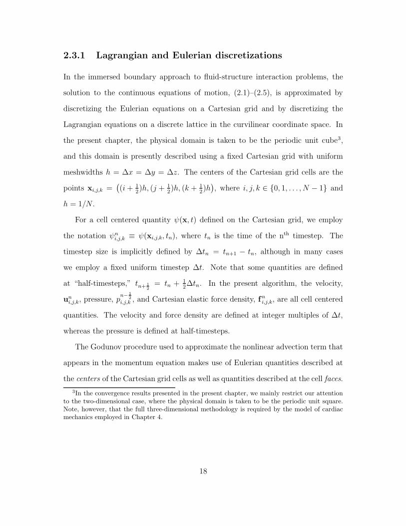
2.3 The uniform grid discretization of the equations of motion . . . . . 17

2.3.1 Lagrangian and Eulerian discretizations . . . . . . . . . . . . 18

2.3.2 Cartesian grid interpolation and finite difference operators . 21

2.3.3 Discrete projection operators . . . . . . . . . . . . . . . . . 25

2.3.4 A discrete curvilinear force density . . . . . . . . . . . . . . 29

2.3.5 Smoothed versions of the Dirac delta function . . . . . . . . 30

2.3.6 Timestepping . . . . . . . . . . . . . . . . . . . . . . . . . . 34

2.3.7 An explicit second order Godunov method . . . . . . . . . . 42

2.3.8 An L-stable scheme for linear parabolic problems . . . . . . 50

2.4 The adaptive discretization of the equations of motion . . . . . . . 54

2.4.1 Hierarchical structured Cartesian grids . . . . . . . . . . . . 54

2.4.2 Interpolation and finite difference operators on locally refined

grids . . . . . . . . . . . . . . . . . . . . . . . . . . . . . . . 61

2.4.3 Timestepping . . . . . . . . . . . . . . . . . . . . . . . . . . 83

2.4.4 Summary of the adaptive algorithm . . . . . . . . . . . . . . 88

2.5 Computational convergence results I: The locally refined projection

method for the incompressible Navier-Stokes equations . . . . . . . 92

2.6 Computational convergence results II: The adaptive version of the

immersed boundary method . . . . . . . . . . . . . . . . . . . . . . 100

2.6.1 Tapered elastic stiffness . . . . . . . . . . . . . . . . . . . . 106

2.6.2 Constant elastic stiffness . . . . . . . . . . . . . . . . . . . . 116

2.7 Hybrid approximate projection methods . . . . . . . . . . . . . . . 120

2.7.1 A more traditional approximate projection method . . . . . 122

2.7.2 Reducing nonphysical pressure oscillations . . . . . . . . . . 123

xii

2.8 Concluding remarks on the adaptive version of the immersed bound-

ary method . . . . . . . . . . . . . . . . . . . . . . . . . . . . . . . 127

3 A parallel implementation of the immersed boundary method for

distributed-memory multiprocessor systems 130

3.1 Basic approaches to distributed-memory parallelization . . . . . . . 130

3.2 Parallel communication and management of Eulerian quantities on

locally refined Cartesian grids . . . . . . . . . . . . . . . . . . . . . 137

3.2.1 Variables, patch data factories, and patch data . . . . . . . . 138

3.2.2 Parallel communication algorithms, operators, and schedules 143

3.2.3 Parallel computing on grid patches . . . . . . . . . . . . . . 145

3.3 Managing the distributed curvilinear mesh . . . . . . . . . . . . . . 158

3.4 Parallel linear solvers . . . . . . . . . . . . . . . . . . . . . . . . . . 166

3.4.1 A necessary condition for the solvability of the composite grid

Poisson problem . . . . . . . . . . . . . . . . . . . . . . . . . 168

3.4.2 The basic multigrid algorithm . . . . . . . . . . . . . . . . . 171

3.4.3 FAC: A composite grid version of the multigrid algorithm . . 177

3.4.4 Implementation issues . . . . . . . . . . . . . . . . . . . . . 184

4 Simulating the blood-muscle-valve mechanics of the heart 187

4.1 An overview of cardiac anatomy and physiology and the model heart 188

4.2 Connecting the model heart to a model of the circulation . . . . . . 191

4.2.1 Modifications to the discrete equations of motion . . . . . . 192

4.2.2 Determining qsrc from a reduced model of the circulation . . 198

4.3 Simulation results . . . . . . . . . . . . . . . . . . . . . . . . . . . . 203

xiii

4.4 Conclusions and directions for future work . . . . . . . . . . . . . . 214

Appendices 218

Bibliography 247

xiv

List of Figures

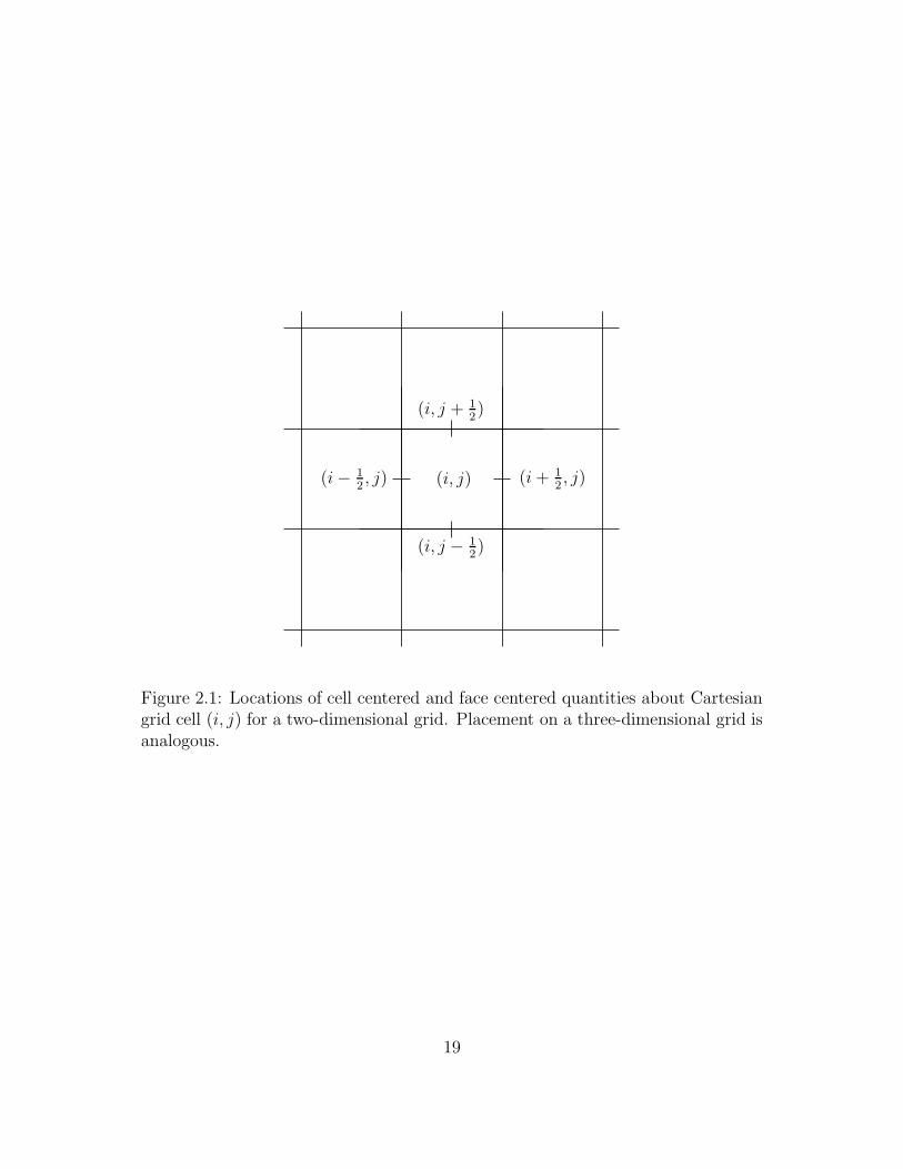
2.1 Locations of cell centered and face centered quantities about Carte-

sian grid cell (i, j) for a two-dimensional grid. Placement on a three-

dimensional grid is analogous. . . . . . . . . . . . . . . . . . . . . . 19

2.2 Three choices among many for φ(r) when constructing a smoothed

approximation to the Dirac delta function using equation (2.43).

These functions are defined by equations (2.49), (2.50), and (2.51),

respectively. . . . . . . . . . . . . . . . . . . . . . . . . . . . . . . . 31

2.3 A properly nested hierarchical structured locally refined Cartesian

grid. Patch boundaries are indicated by bold lines. Each level in the

patch hierarchy consists of one or more rectangular grid patches, and

the levels satisfy the proper nesting condition. Here, the refinement

ratio is r = 2. (Compare to the improperly nested configuration of

Figure 2.4.) . . . . . . . . . . . . . . . . . . . . . . . . . . . . . . . 56

2.4 An improperly nested hierarchical structured locally refined Carte-

sian grid. This configuration is improperly nested because unrefined

cells of level 0 are directly adjacent to cells of level 2. (Compare to

the properly nested configuration of Figure 2.3.) . . . . . . . . . . . 57

xv

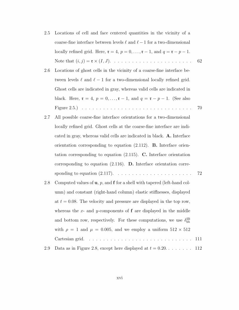
2.5 Locations of cell and face centered quantities in the vicinity of a

coarse-fine interface between levels ` and `− 1 for a two-dimensional

locally refined grid. Here, r = 4, p = 0, . . . , r− 1, and q = r− p− 1.

Note that (i, j) = r× (I, J). . . . . . . . . . . . . . . . . . . . . . . 62

2.6 Locations of ghost cells in the vicinity of a coarse-fine interface be-

tween levels ` and ` − 1 for a two-dimensional locally refined grid.

Ghost cells are indicated in gray, whereas valid cells are indicated in

black. Here, r = 4, p = 0, . . . , r − 1, and q = r − p − 1. (See also

Figure 2.5.) . . . . . . . . . . . . . . . . . . . . . . . . . . . . . . . 70

2.7 All possible coarse-fine interface orientations for a two-dimensional

locally refined grid. Ghost cells at the coarse-fine interface are indi-

cated in gray, whereas valid cells are indicated in black. A. Interface

orientation corresponding to equation (2.112). B. Interface orien-

tation corresponding to equation (2.115). C. Interface orientation

corresponding to equation (2.116). D. Interface orientation corre-

sponding to equation (2.117). . . . . . . . . . . . . . . . . . . . . . 72

2.8 Computed values of u, p, and f for a shell with tapered (left-hand col-

umn) and constant (right-hand column) elastic stiffnesses, displayed

at t = 0.08. The velocity and pressure are displayed in the top row,

whereas the x- and y-components of f are displayed in the middle

and bottom row, respectively. For these computations, we use δIB6h

with ρ = 1 and µ = 0.005, and we employ a uniform 512 × 512

Cartesian grid. . . . . . . . . . . . . . . . . . . . . . . . . . . . . . 111

2.9 Data as in Figure 2.8, except here displayed at t = 0.20. . . . . . . . 112

xvi

2.10 Data as in Figure 2.8, except here displayed at t = 0.32. . . . . . . . 113

2.11 Location of a shell with tapered (left-hand column) and constant

(right-hand column) elastic stiffnesses at A. t = 0.08, B. t = 0.20,

and C. t = 0.32 for an adaptive computation using δIB6h. In all cases,

level 0 consists of a single 128× 128 grid patch, and the refinement

ratio is r = 4. The volume occupied by the shell is indicated in gray,

and fine grid patches are indicated by thick black lines. Note that

the refined regions in the Cartesian grid are placed adaptively and

to cover the elastic structure completely. . . . . . . . . . . . . . . . 114

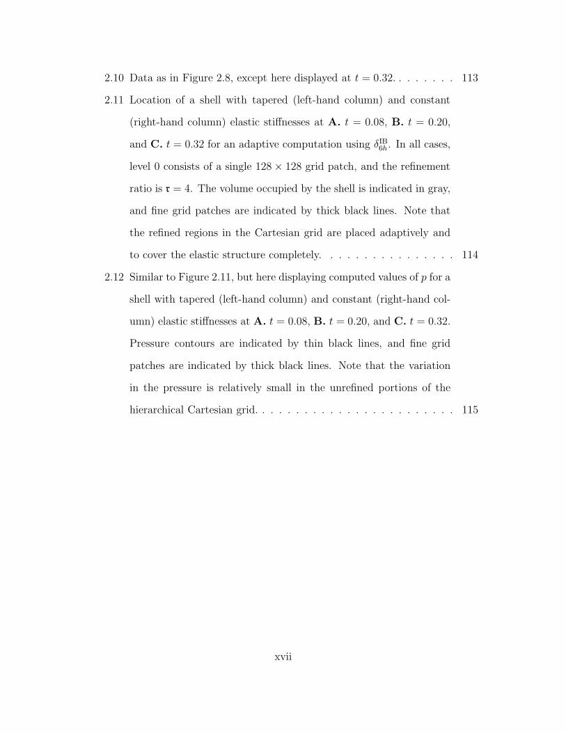
2.12 Similar to Figure 2.11, but here displaying computed values of p for a

shell with tapered (left-hand column) and constant (right-hand col-

umn) elastic stiffnesses at A. t = 0.08, B. t = 0.20, and C. t = 0.32.

Pressure contours are indicated by thin black lines, and fine grid

patches are indicated by thick black lines. Note that the variation

in the pressure is relatively small in the unrefined portions of the

hierarchical Cartesian grid. . . . . . . . . . . . . . . . . . . . . . . . 115

xvii

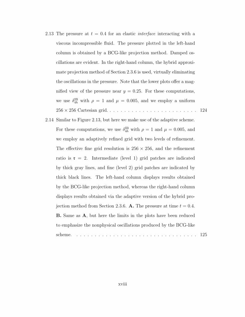
2.13 The pressure at t = 0.4 for an elastic interface interacting with a

viscous incompressible fluid. The pressure plotted in the left-hand

column is obtained by a BCG-like projection method. Damped os-

cillations are evident. In the right-hand column, the hybrid approxi-

mate projection method of Section 2.3.6 is used, virtually eliminating

the oscillations in the pressure. Note that the lower plots offer a mag-

nified view of the pressure near y = 0.25. For these computations,

we use δIB4h with ρ = 1 and µ = 0.005, and we employ a uniform

256× 256 Cartesian grid. . . . . . . . . . . . . . . . . . . . . . . . . 124

2.14 Similar to Figure 2.13, but here we make use of the adaptive scheme.

For these computations, we use δIB4h with ρ = 1 and µ = 0.005, and

we employ an adaptively refined grid with two levels of refinement.

The effective fine grid resolution is 256 × 256, and the refinement

ratio is r = 2. Intermediate (level 1) grid patches are indicated

by thick gray lines, and fine (level 2) grid patches are indicated by

thick black lines. The left-hand column displays results obtained

by the BCG-like projection method, whereas the right-hand column

displays results obtained via the adaptive version of the hybrid pro-

jection method from Section 2.3.6. A. The pressure at time t = 0.4.

B. Same as A, but here the limits in the plots have been reduced

to emphasize the nonphysical oscillations produced by the BCG-like

scheme. . . . . . . . . . . . . . . . . . . . . . . . . . . . . . . . . . 125

xviii

3.1 SAMRAI provides several predefined patch data objects that each

implement the standard PatchData interface. The parallel commu-

nication and data management capabilities provided by the SAM-

RAI library also support the introduction of application-specific data

types, and we make use of this ability in our implementation of the

adaptive version of the immersed boundary method. . . . . . . . . . 141

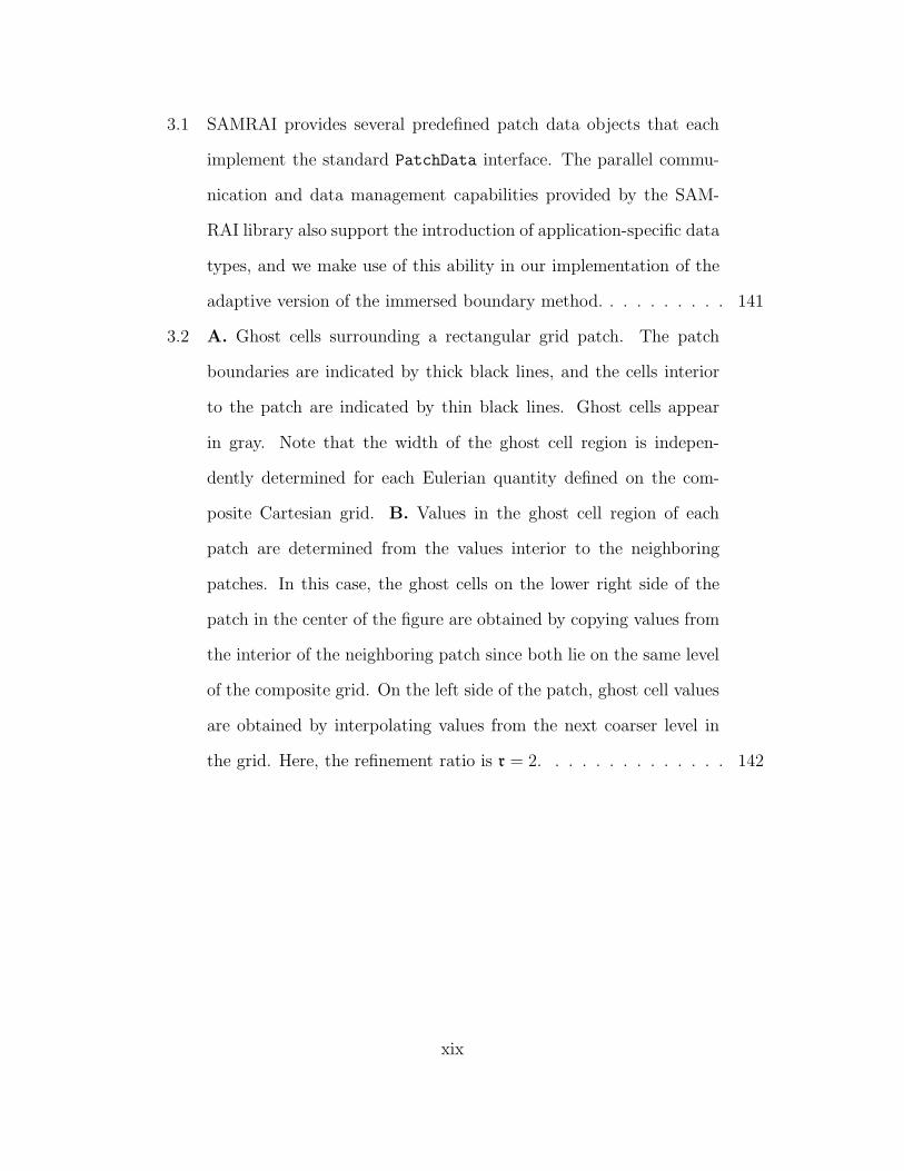
3.2 A. Ghost cells surrounding a rectangular grid patch. The patch

boundaries are indicated by thick black lines, and the cells interior

to the patch are indicated by thin black lines. Ghost cells appear

in gray. Note that the width of the ghost cell region is indepen-

dently determined for each Eulerian quantity defined on the com-

posite Cartesian grid. B. Values in the ghost cell region of each

patch are determined from the values interior to the neighboring

patches. In this case, the ghost cells on the lower right side of the

patch in the center of the figure are obtained by copying values from

the interior of the neighboring patch since both lie on the same level

of the composite grid. On the left side of the patch, ghost cell values

are obtained by interpolating values from the next coarser level in

the grid. Here, the refinement ratio is r = 2. . . . . . . . . . . . . . 142

xix

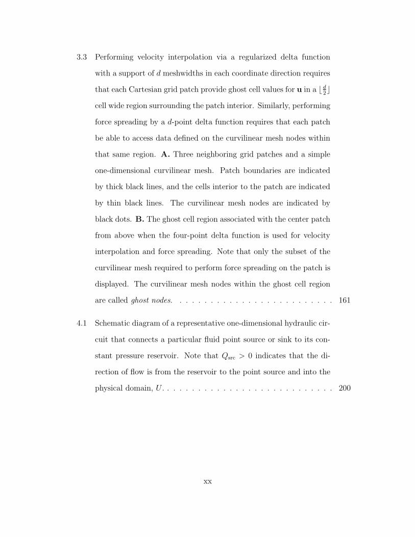
3.3 Performing velocity interpolation via a regularized delta function

with a support of d meshwidths in each coordinate direction requires

that each Cartesian grid patch provide ghost cell values for u in a b d2c

cell wide region surrounding the patch interior. Similarly, performing

force spreading by a d-point delta function requires that each patch

be able to access data defined on the curvilinear mesh nodes within

that same region. A. Three neighboring grid patches and a simple

one-dimensional curvilinear mesh. Patch boundaries are indicated

by thick black lines, and the cells interior to the patch are indicated

by thin black lines. The curvilinear mesh nodes are indicated by

black dots. B. The ghost cell region associated with the center patch

from above when the four-point delta function is used for velocity

interpolation and force spreading. Note that only the subset of the

curvilinear mesh required to perform force spreading on the patch is

displayed. The curvilinear mesh nodes within the ghost cell region

are called ghost nodes. . . . . . . . . . . . . . . . . . . . . . . . . . 161

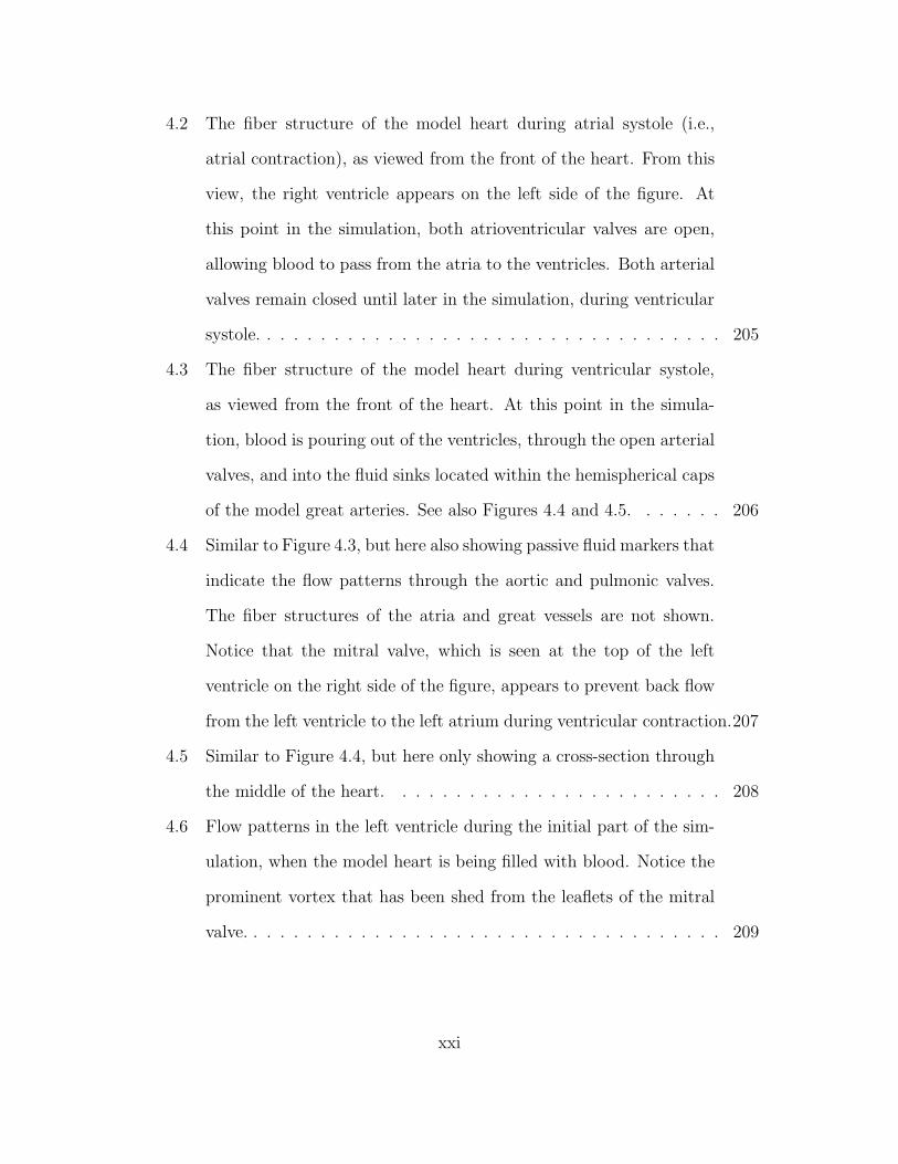
4.1 Schematic diagram of a representative one-dimensional hydraulic cir-

cuit that connects a particular fluid point source or sink to its con-

stant pressure reservoir. Note that Qsrc > 0 indicates that the di-

rection of flow is from the reservoir to the point source and into the

physical domain, U . . . . . . . . . . . . . . . . . . . . . . . . . . . . 200

xx

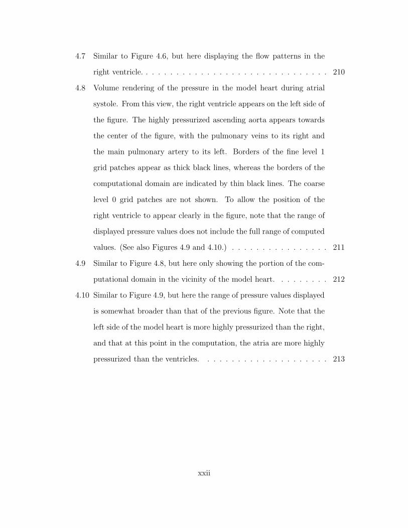
4.2 The fiber structure of the model heart during atrial systole (i.e.,

atrial contraction), as viewed from the front of the heart. From this

view, the right ventricle appears on the left side of the figure. At

this point in the simulation, both atrioventricular valves are open,

allowing blood to pass from the atria to the ventricles. Both arterial

valves remain closed until later in the simulation, during ventricular

systole. . . . . . . . . . . . . . . . . . . . . . . . . . . . . . . . . . . 205

4.3 The fiber structure of the model heart during ventricular systole,

as viewed from the front of the heart. At this point in the simula-

tion, blood is pouring out of the ventricles, through the open arterial

valves, and into the fluid sinks located within the hemispherical caps

of the model great arteries. See also Figures 4.4 and 4.5. . . . . . . 206

4.4 Similar to Figure 4.3, but here also showing passive fluid markers that

indicate the flow patterns through the aortic and pulmonic valves.

The fiber structures of the atria and great vessels are not shown.

Notice that the mitral valve, which is seen at the top of the left

ventricle on the right side of the figure, appears to prevent back flow

from the left ventricle to the left atrium during ventricular contraction.207

4.5 Similar to Figure 4.4, but here only showing a cross-section through

the middle of the heart. . . . . . . . . . . . . . . . . . . . . . . . . 208

4.6 Flow patterns in the left ventricle during the initial part of the sim-

ulation, when the model heart is being filled with blood. Notice the

prominent vortex that has been shed from the leaflets of the mitral

valve. . . . . . . . . . . . . . . . . . . . . . . . . . . . . . . . . . . . 209

xxi

4.7 Similar to Figure 4.6, but here displaying the flow patterns in the

right ventricle. . . . . . . . . . . . . . . . . . . . . . . . . . . . . . . 210

4.8 Volume rendering of the pressure in the model heart during atrial

systole. From this view, the right ventricle appears on the left side of

the figure. The highly pressurized ascending aorta appears towards

the center of the figure, with the pulmonary veins to its right and

the main pulmonary artery to its left. Borders of the fine level 1

grid patches appear as thick black lines, whereas the borders of the

computational domain are indicated by thin black lines. The coarse

level 0 grid patches are not shown. To allow the position of the

right ventricle to appear clearly in the figure, note that the range of

displayed pressure values does not include the full range of computed

values. (See also Figures 4.9 and 4.10.) . . . . . . . . . . . . . . . . 211

4.9 Similar to Figure 4.8, but here only showing the portion of the com-

putational domain in the vicinity of the model heart. . . . . . . . . 212

4.10 Similar to Figure 4.9, but here the range of pressure values displayed

is somewhat broader than that of the previous figure. Note that the

left side of the model heart is more highly pressurized than the right,

and that at this point in the computation, the atria are more highly

pressurized than the ventricles. . . . . . . . . . . . . . . . . . . . . 213

xxii

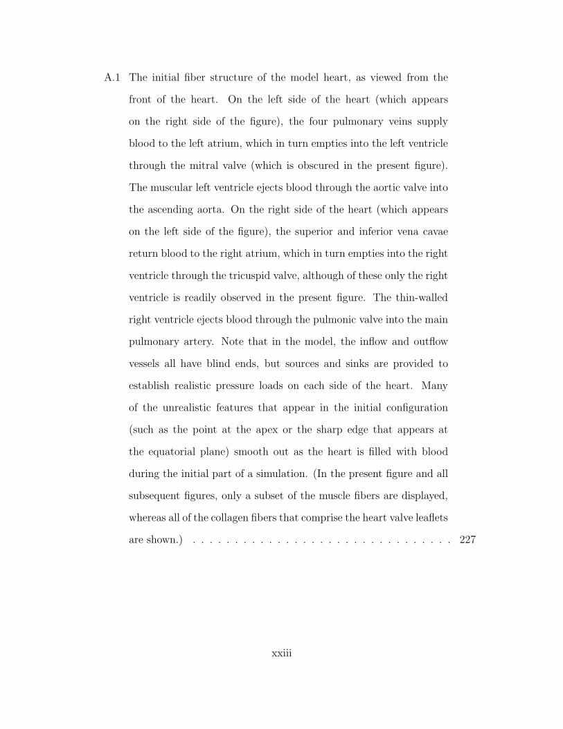
A.1 The initial fiber structure of the model heart, as viewed from the

front of the heart. On the left side of the heart (which appears

on the right side of the figure), the four pulmonary veins supply

blood to the left atrium, which in turn empties into the left ventricle

through the mitral valve (which is obscured in the present figure).

The muscular left ventricle ejects blood through the aortic valve into

the ascending aorta. On the right side of the heart (which appears

on the left side of the figure), the superior and inferior vena cavae

return blood to the right atrium, which in turn empties into the right

ventricle through the tricuspid valve, although of these only the right

ventricle is readily observed in the present figure. The thin-walled

right ventricle ejects blood through the pulmonic valve into the main

pulmonary artery. Note that in the model, the inflow and outflow

vessels all have blind ends, but sources and sinks are provided to

establish realistic pressure loads on each side of the heart. Many

of the unrealistic features that appear in the initial configuration

(such as the point at the apex or the sharp edge that appears at

the equatorial plane) smooth out as the heart is filled with blood

during the initial part of a simulation. (In the present figure and all

subsequent figures, only a subset of the muscle fibers are displayed,

whereas all of the collagen fibers that comprise the heart valve leaflets

are shown.) . . . . . . . . . . . . . . . . . . . . . . . . . . . . . . . 227

xxiii

A.2 The ventricular muscle fibers of the model heart, as viewed from the

front of the heart, so that the right ventricle again appears on the left

side of the figure. The present figure includes the outer/inner layer,

the right-inner/left-outer layer, and the internal left-ventricular lay-

ers described in Appendix A. The four coplanar valve rings are

indicated by black markers and form the base of the heart. From

this view, the aortic valve ring appears near the center of the figure,

with the pulmonic valve ring appearing slightly below and to the

left. The larger mitral and tricuspid valve rings appear respectively

to the right and back of the aortic valve ring. (As before, only a

subset of model muscle fibers are displayed.) . . . . . . . . . . . . . 228

A.3 The four nested internal left-ventricular layers of the model heart

described in Appendix A, as viewed from the front of the heart.

The valve rings are again indicated by black markers. The larger

mitral valve ring is the location at which the left atrium joins the

left ventricle, whereas the smaller aortic valve ring is the location at

which the ascending aorta is attached. (As before, only a subset of

model muscle fibers are displayed.) . . . . . . . . . . . . . . . . . . 229

A.4 Similar to Figure A.3, but here only showing three of the nested

internal left-ventricular layers . . . . . . . . . . . . . . . . . . . . . 230

A.5 Similar to Figure A.3, but here only showing two of the nested in-

ternal left-ventricular layers . . . . . . . . . . . . . . . . . . . . . . 230

A.6 Similar to Figure A.3, but here only showing one of the nested in-

ternal left-ventricular layers . . . . . . . . . . . . . . . . . . . . . . 231

xxiv

A.7 The inflow structures of the model heart, viewed from the right side

of the heart. The superior and inferior vena cavae appear on the

left side of the figure and are connected to the right atrium. The

right atrium empties through the tricuspid valve (which appears in

the figure to the right of the inferior vena cava) into the right ven-

tricle (not shown). Corresponding structures on the left side of the

heart appear on the right side of the figure. They include the four

pulmonary veins, the left atrium, and the left atrial appendage (au-

ricle). The left atrium empties through the mitral valve (which ap-

pears below the left atrium and to the left of the auricle) into the

left ventricle (not shown). Both the tricuspid valve and the mitral

valve are supported by fans of chordae tendineae, which in turn in-

sert into papillary muscles. (As before, except for the case of the

valve leaflets, only a subset of model fibers are displayed.) . . . . . 232

A.8 The four valves of the model heart viewed from above (i.e., looking

from the arterial side towards the ventricles). Note that the fiber

structure of both outflow (aortic and pulmonic) valves is identical,

although their elastic properties differ in accordance with the differ-

ent pressure loads each is required to support. . . . . . . . . . . . . 233

xxv

A.9 The four valves of the model heart, as viewed from the front of the

heart. From this view, the outflow (aortic and pulmonic) valves

appear above the inflow (mitral and tricuspid) valves. The pulmonic

valve is located above the aortic valve, and the mitral valve is located

to the right of the tricuspid valve. Note that the inflow valves are

supported by fans of chordae tendineae which insert into papillary

muscles, whereas the outflow valves are self-supporting. . . . . . . . 234

A.10 A. Surface rendering of the initial closed-valve configuration of the

model aortic heart valve leaflets. The structure of the model pul-

monic valve is identical, although it has different elastic proper-

ties that reflect the lower pressures developed by the right ventricle.

B. Similar to A, but here the curvilinear mesh that defines the initial

configuration of the valve is also shown. . . . . . . . . . . . . . . . . 235

xxvi

List of Algorithms

2.1 Evaluate u = Af→cuMAC on all levels of the patch hierarchy. . . . . 65

2.2 Evaluate Df→c · uMAC on all levels of the patch hierarchy. . . . . . . 65

2.3 Evaluate uMAC = Ac→fu on all levels of the patch hierarchy. . . . . 77

2.4 Evaluate Gc→fψ on all levels of the patch hierarchy. . . . . . . . . . 78

2.5 Simultaneously compute the approximate projection of u∗ and the

exact projection of uMAC,∗ = Ac→fu∗. . . . . . . . . . . . . . . . . . 91

3.1 The basic multigrid V-cycle for computing an approximate solution,

v, to the linear system of equations Lu = f on a uniform grid. . . . 175

3.2 The main FAC solver loop for computing an approximate solution,

v, to the linear system of equations Lu = f on a composite grid. . . 179

3.3 The composite grid generalization of the multigrid V-cycle for com-

puting an approximate solution, e, to the linear system of equations

Le = r on each level of a composite grid. . . . . . . . . . . . . . . . 179

3.4 The grid patch-based smoother employed in the inner FAC V-cycle. 182

xxvii

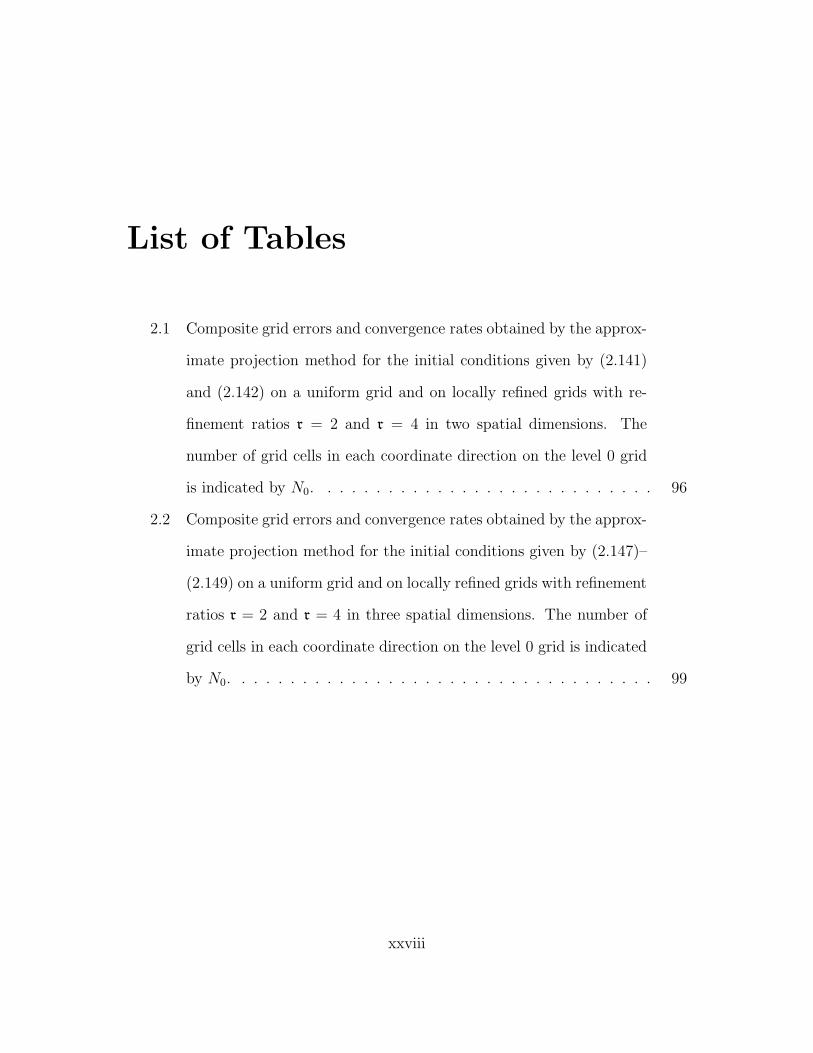
List of Tables

2.1 Composite grid errors and convergence rates obtained by the approx-

imate projection method for the initial conditions given by (2.141)

and (2.142) on a uniform grid and on locally refined grids with re-

finement ratios r = 2 and r = 4 in two spatial dimensions. The

number of grid cells in each coordinate direction on the level 0 grid

is indicated by N0. . . . . . . . . . . . . . . . . . . . . . . . . . . . 96

2.2 Composite grid errors and convergence rates obtained by the approx-

imate projection method for the initial conditions given by (2.147)–

(2.149) on a uniform grid and on locally refined grids with refinement

ratios r = 2 and r = 4 in three spatial dimensions. The number of

grid cells in each coordinate direction on the level 0 grid is indicated

by N0. . . . . . . . . . . . . . . . . . . . . . . . . . . . . . . . . . . 99

xxviii

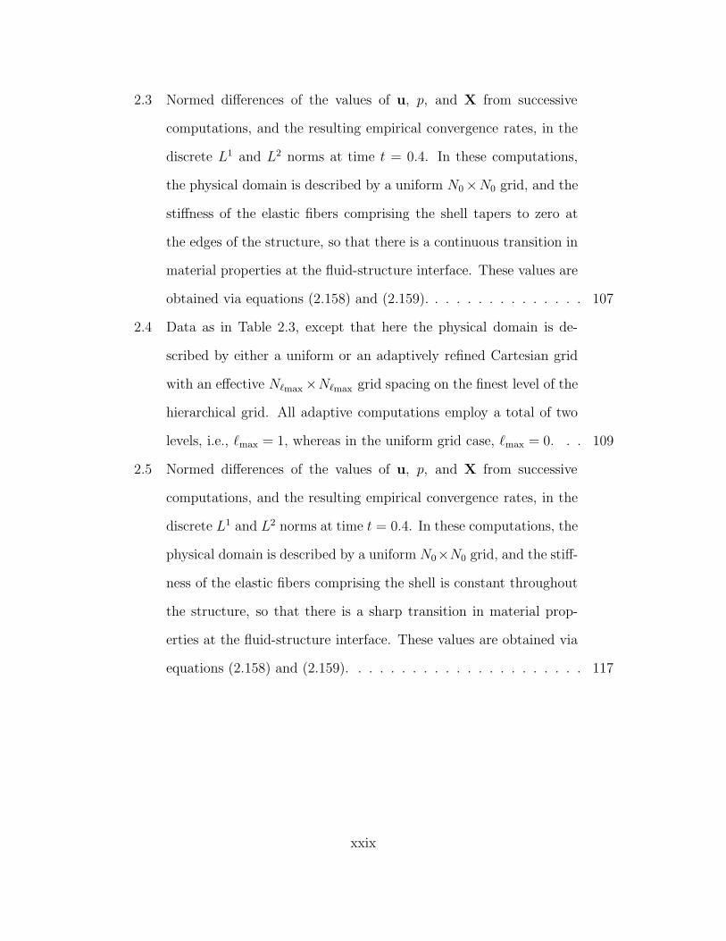
2.3 Normed differences of the values of u, p, and X from successive

computations, and the resulting empirical convergence rates, in the

discrete L1 and L2 norms at time t = 0.4. In these computations,

the physical domain is described by a uniform N0×N0 grid, and the

stiffness of the elastic fibers comprising the shell tapers to zero at

the edges of the structure, so that there is a continuous transition in

material properties at the fluid-structure interface. These values are

obtained via equations (2.158) and (2.159). . . . . . . . . . . . . . . 107

2.4 Data as in Table 2.3, except that here the physical domain is de-

scribed by either a uniform or an adaptively refined Cartesian grid

with an effective N`max×N`max grid spacing on the finest level of the

hierarchical grid. All adaptive computations employ a total of two

levels, i.e., `max = 1, whereas in the uniform grid case, `max = 0. . . 109

2.5 Normed differences of the values of u, p, and X from successive

computations, and the resulting empirical convergence rates, in the

discrete L1 and L2 norms at time t = 0.4. In these computations, the

physical domain is described by a uniform N0×N0 grid, and the stiff-

ness of the elastic fibers comprising the shell is constant throughout

the structure, so that there is a sharp transition in material prop-

erties at the fluid-structure interface. These values are obtained via

equations (2.158) and (2.159). . . . . . . . . . . . . . . . . . . . . . 117

xxix

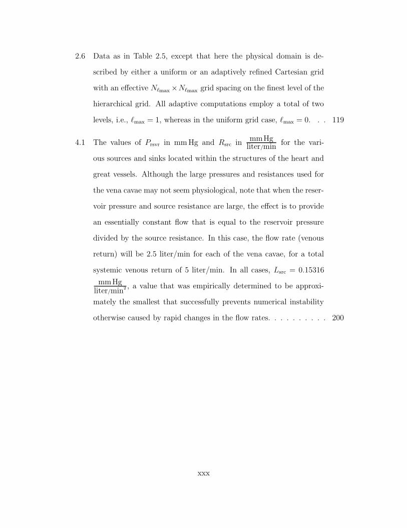
2.6 Data as in Table 2.5, except that here the physical domain is de-

scribed by either a uniform or an adaptively refined Cartesian grid

with an effective N`max×N`max grid spacing on the finest level of the

hierarchical grid. All adaptive computations employ a total of two

levels, i.e., `max = 1, whereas in the uniform grid case, `max = 0. . . 119

4.1 The values of Prsvr in mm Hg and Rsrc inmmHg

liter/minfor the vari-

ous sources and sinks located within the structures of the heart and

great vessels. Although the large pressures and resistances used for

the vena cavae may not seem physiological, note that when the reser-

voir pressure and source resistance are large, the effect is to provide

an essentially constant flow that is equal to the reservoir pressure

divided by the source resistance. In this case, the flow rate (venous

return) will be 2.5 liter/min for each of the vena cavae, for a total

systemic venous return of 5 liter/min. In all cases, Lsrc = 0.15316

mmHgliter/min2 , a value that was empirically determined to be approxi-

mately the smallest that successfully prevents numerical instability

otherwise caused by rapid changes in the flow rates. . . . . . . . . . 200

xxx

List of Appendices

A A three-dimensional fiber model of the heart 218

B Incompressible fluid dynamics with distributed sources and sinks236

B.1 The modified equations of motion . . . . . . . . . . . . . . . . . . . 237

B.2 The rate of dissipation of kinetic energy associated with fluid sources

and sinks . . . . . . . . . . . . . . . . . . . . . . . . . . . . . . . . 241

B.3 Summary of the equations of motion . . . . . . . . . . . . . . . . . 245

xxxi

Chapter 1

Introduction

The heart consists of two pumps—the right and left sides of the heart—that are

responsible for pumping blood through the lungs and through the peripheral organs,

respectively. Each side of the heart consists of two chambers, an atrium and a

ventricle, with the weaker atrium acting as a receiving chamber and as a primer

pump for the more powerful ventricle. In a normal heartbeat, the contraction

of the atria is followed after a brief delay (approximately one-sixth of a second)

by the contraction of the ventricles. These muscle contractions are stimulated

by electrical currents that flow through the heart tissue and are coordinated by

a specialized conduction system. This conduction system additionally allows the

ventricles to contract nearly synchronously, thereby ensuring that the heart is able

to effectively generate the high pressures required to pump blood to all the tissues

of the body. It should not be surprising, then, that arrhythmic excitation patterns

or abnormalities in the structure of the heart can pose serious health risks. In fact,

since 1900, cardiovascular diseases have been the leading causes of death in the

1

United States every year but 1918 [5].

Computer simulation can provide a means for studying both the normal and

diseased heart, providing detailed spatial and temporal data that may not be easily

obtained by experiment. Simulations also allow for systematic parameter studies

and thus can be used to aid the design of medical devices such as artificial heart

valves. Damage or destruction of the heart valve leaflets, most often caused by

autoimmune diseases or congenital defects, can lead to stenosis (where the flow

resistance of the valve becomes too large) or incompetence (where the valve becomes

leaky, allowing regurgitation). In either case, the normal functioning of the heart is

impaired, and in severe cases valve repair or replacement is required. Approximately

250,000 such operations are performed annually, and of these surgeries, roughly

180,000 involve the implanting of replacement valves [81]. Unfortunately, modern

prosthetic valves can result in several serious complications, many of which are

closely related to the the flow of blood in and around the replacement valve. For

instance, artificial valves may produce more turbulent flow patterns than those

yielded by healthy natural valves. Such turbulent flows can cause lethal damage to

red blood cells and may result in platelet activation. By contrast, prosthetic valves

may also produce new regions of flow stagnation, which can result in thrombus

formation, tissue overgrowth, and calcification. (For a more complete discussion

of these issues, the reader is refereed to, e.g., [81].) The design of artificial heart

valves can be posed as an optimization problem [48, 50], and numerical optimization

methods can be employed to determine valve shapes that, say, maximize flow rates

while minimizing regurgitation, stagnation, and turbulent shear stresses. However,

medically useful solutions to such problems will require detailed simulations of the

2

interaction of blood flow with the thin heart valve leaflets, the muscular heart wall,

and the nearby great vessels.

The present work focuses on the description and implementation of an adaptive

numerical method for simulating fluid-structure interaction, a method that we in

turn apply to the computer simulation cardiac mechanics. More specifically, we

introduce a new adaptive and parallel version of the immersed boundary method

and apply this methodology to Peskin and McQueen’s three-dimensional model of

the heart and great vessels [62, 49, 64, 52, 53]. In this model, the blood is described

as a viscous incompressible fluid, and the valves of the heart and the muscular

heart walls are described as elastic or viscoelastic structures. As we describe in

Chapter 2, the immersed boundary method is a mathematical formulation and

numerical approach to such problems.

Simulating blood flow in the heart by the immersed boundary method requires

the use of high spatial resolution; however, this requirement is somewhat localized

to the flow in the neighborhood of the immersed boundaries, i.e., the heart valve

leaflets, the muscular heart walls, and the walls of the great vessels. For the flow

within the chambers of the heart but away from the immersed boundaries, the

need for high spatial resolution is somewhat lessened, although it may be needed

in regions of high vorticity in the interior of the flow, i.e., in the neighborhood of

vortices that have been shed from the boundaries, particularly from the free edges

of the heart valve leaflets, and have subsequently moved away from the boundaries

into the interior of the flow. In the model of Peskin and McQueen, there is also flow

in the region exterior to the heart, although it seems plausible that it would suffice

to employ comparatively coarse resolution in this portion of the computational

3

domain.

For problems that possess localized fine-scale features, computational resources

are more efficiently utilized by employing adaptive techniques, whereby high spatial

resolution is deployed locally where it is most needed and comparatively coarse reso-

lution is employed where it suffices. In Chapter 2, we describe a particular adaptive

version of the immersed boundary method. Although this adaptive scheme employs

the same hierarchical structured grid approach as an earlier two-dimensional adap-

tive immersed boundary method introduced by Roma, Peskin, and Berger [66, 67],

the numerical algorithm employed in the present work is based on a non-adaptive,

formally second order accurate version of the immersed boundary method that we

recently introduced [29]. Like the uniform grid algorithm upon which it is based,

the new adaptive method is formally second order accurate in the sense that the

method is expected to converge at its formal order of accuracy only for problems

with a sufficiently smooth solution. By considering such a problem, namely the in-

teraction of a viscous incompressible fluid and a viscoelastic shell, we obtain actual

second order convergence rates with both the uniform and adaptive methods.

Despite decades of sustained growth in computing power, three-dimensional

heart simulation via the immersed boundary method continues to require the use

of large parallel computers. To make use of such platforms in their work, Peskin

and McQueen developed a parallel version of the immersed boundary method [51];

however, their computational framework was carefully optimized for the types of

machines that were most widely available at the time of its original development,

namely shared-memory parallel computers comprised of tens of vector processors.

Most recent supercomputers typically consist of hundreds, thousands, or even tens

4

of thousands of processors and do not provide a global address space. To take advan-

tage of modern parallel computers, we have implemented a new distributed-memory

parallel version of the immersed boundary method that is described in Chapter 3.

The resulting software is both sufficiently efficient to be useful for performing “pro-

duction level” simulations and sufficiently flexible to serve as a platform for the

continued development of new numerical methods. Accomplishing these twin goals

was made more manageable by employing modern software design principles [27]

and, as we discuss in some detail, by using readily available mathematical software

libraries.

Finally, in Chapter 4, we present initial computational results obtained from the

application of the adaptive and parallel implementation of the immersed boundary

method to Peskin and McQueen’s three-dimensional model of cardiac mechanics.

Although this work is not yet complete, we believe that the simulation results

obtained so far demonstrate that we have already begun to utilize effectively the

adaptive and distributed-parallel capabilities provided by this new version of the

immersed boundary method.

5

Chapter 2

An adaptive immersed boundary

method for fluid-structure

interaction

2.1 Introduction and relationship to prior work

Like many problems in biofluid mechanics, cardiac mechanics can be modeled

as the dynamic interaction of a viscous incompressible fluid (the blood) and a

(visco-)elastic structure (the muscular walls and the valves of the heart). The im-

mersed boundary method is a mathematical formulation and numerical approach

to such problems originally introduced by Peskin to study blood flow through heart

valves [57, 58]. In the formulation of the problem introduced by Peskin and ex-

tended by Peskin and McQueen [62, 49, 59, 63, 64, 52, 53], the blood is modeled

as a viscous incompressible fluid, whereas the muscular heart wall is modeled as a

6

thick viscoelastic structure and the flexible heart valve leaflets are modeled as thin

elastic boundaries.

In the immersed boundary formulation of problems involving the interaction of

a viscous incompressible fluid and an elastic or viscoelastic structure, the configu-

ration of the elastic structure is described by Lagrangian variables (i.e., variables

indexed by a coordinate system attached to the elastic structure), whereas the mo-

mentum, velocity, and incompressibility of the coupled fluid-structure system are

described by Eulerian variables (i.e., in reference to fixed physical coordinates).

In the continuous equations of motion, these two descriptions are connected by

making use of the Dirac delta function, whereas a smoothed approximation to the

delta function is used to link the Lagrangian and Eulerian descriptions when the

continuous equations are discretely approximated for computer simulation.

When the immersed boundary method is used to simulate blood flow in the

heart, high spatial resolution is required, especially in the vicinity of the heart

valve leaflets. If a uniform grid is employed to discretize the (Eulerian) equations

of motion for such a simulation, the fine grid spacing required to resolve the flow

through the valves is necessarily employed throughout the entire computational

domain, even in regions that may not require such high resolution (e.g., exterior

to the heart). By employing an adaptive discretization of the equations of motion,

high spatial resolution can be deployed locally where it is most needed, whereas

comparatively coarse resolution can be employed where it suffices. In principle,

such an adaptive scheme would allow for more efficient utilization of computational

resources when compared to non-adaptive strategies. Realizing such gains in prac-

tice requires the careful design and implementation of a number of algorithms and

7

data structures.

An adaptive version of the immersed boundary method was first introduced in

the Ph.D. thesis of A. M. Roma [66] and the subsequent work of Roma, Peskin,

and Berger [67]. In this work, the hierarchical structured grid approach of Berger

and Oliger [13] and Berger and Colella [12] was employed to introduce local spatial

refinement in the Eulerian grid in the vicinity of an immersed elastic interface. Note

that this adaptive version of the immersed boundary method was found to produce

dynamics that were not significantly different from those obtained by a non-adaptive

method that employed a uniform grid with the same spatial resolution as that of

the finest grid level in the adaptive computation.

The present chapter focuses on describing a new adaptive version of the im-

mersed boundary method for fluid-structure interaction problems. This adaptive

method is based upon a non-adaptive, formally second order accurate version of the

immersed boundary method recently described by Griffith and Peskin [29]. Like

the uniform grid algorithm upon which it is based, this new adaptive version of

the immersed boundary method is formally second order accurate in the sense that

the method is expected to converge at its formal order of accuracy only for prob-

lems with a sufficiently smooth solution. The present adaptive algorithm employs

the same hierarchical structured grid approach (but a different numerical scheme,

see below) as that used by Roma, Peskin, and Berger to discretize the Eulerian

equations of motion (i.e., the incompressible Navier-Stokes equations). Unlike the

method of Roma et al., the present algorithm employs a fully explicit treatment of

the Lagrangian equations of motion (i.e., the equations that specify the evolution

of the configuration of the elastic structure). In particular, in an attempt to reduce

8

the occurrence of nonphysical oscillations in the computed dynamics, we employ a

strong stability-preserving Runge-Kutta method [28] for the time integration of the

Lagrangian equations of motion.

The present method differs more dramatically from the approach of Roma et

al. in the details of its treatment of the Eulerian equations of motion, namely the

incompressible Navier-Stokes equations. Although both adaptive schemes employ

projection methods to solve the incompressible Navier-Stokes equations, the present

work employs a cell centered projection method that makes use of an implicit L-

stable discretization of the viscous terms [78, 47] and a second order Godunov

method for the explicit treatment of the nonlinear advection terms [20, 54, 55, 42].

Generally speaking, projection methods [18, 19, 11] are a class of fractional step

algorithms for incompressible flow problems that update the velocity by first solving

the momentum equation over a time interval without imposing the constraint of

incompressibility. Doing so yields an “intermediate” velocity field that is generally

not divergence free. The “true” updated velocity is then obtained by solving a

Poisson problem to enforce the incompressibility constraint. More abstractly, this

process projects the intermediate velocity onto the space of divergence free vector

fields.

In an “exact” projection method, the discrete divergence of the updated velocity

is identically zero (in exact arithmetic, and zero to within the tolerance of the

linear solver in practice). However, even on uniform grids, exact cell centered

projections present difficulties. For example, on a periodic grid with an even number

of grid cells in each coordinate direction, an exact projection operator possesses a

nontrivial nullspace that causes the pressure to decouple into 2d subfields, where d

9

is the number of spatial dimensions. To date, it appears that exact cell centered

projections have not been successfully implemented for co-located cell centered

velocities defined on hierarchically composed locally refined grids (i.e., such as those

used in the present work). Like most recent projection methods for locally refined

grids [55, 2, 42], the present method employs a projection method that is not exact

but rather is “approximate” in the sense that the discrete divergence of the velocity

only converges to zero at a second order rate as the composite computational grid

is refined. (Note that unlike exact projection methods, approximate projection

methods typically yield a fully coupled pressure field on both uniform and locally

refined grids.) When such methods are used with the immersed boundary method,

we have found that it is beneficial to determine the updated velocity and pressure

in terms of the solutions to two different approximate projection equations at each

timestep. This so-called hybrid approach was originally proposed by Almgren et

al. for simulating inviscid incompressible flow [3]. Our approach, which we first

detailed in [29], is essentially an extension of their algorithm (“version 5”) to the

viscous case.

Most traditional projection methods only employ a single projection at each

timestep to determine both the updated velocity and the updated pressure. Conse-

quently, when compared to such traditional projection algorithms, hybrid methods

require the solution of additional systems of linear equations at each timestep, al-

though this additional expense can be made modest. In the context of the immersed

boundary method, we have found that the use of a more traditional projection

method can introduce spurious oscillations in the computed pressure even in the

uniform grid case. These oscillations are exacerbated in the presence of local mesh

10

refinement. Though such oscillations are sometimes described as hallmarks of the

immersed boundary method [39], the hybrid approach that we employ virtually

eliminates these pressure oscillations both for uniform grid and adaptive compu-

tations. Moreover, these improvements are observed both for problems involving

thin elastic interfaces as well as for problems modeling thicker structures such as

viscoelastic shells.

Projection methods for locally refined grids fall into one of two categories: meth-

ods that employ a uniform timestep over the entire range of levels composing the

composite grid [55, 34], and methods that refine the timestep at the same rate as

the spatial grid spacing (i.e., methods that employ subcycling in time) [2, 42]. Al-

though it has been estimated that projection methods that synchronously advance

all levels of the grid hierarchy are less efficient than schemes employing subcycling

in time [2], the present method takes the former approach for ease of implemen-

tation. We have tried to design our present implementation in such a way that

subcycling in time can be introduced without too much additional effort, but we

leave the full implementation and study of subcycling in the immersed boundary

context for future research.

As in the uniform grid method of [29], actual second order numerical convergence

rates are observed when the adaptive method is used to simulate the interaction of

a viscous incompressible fluid and a viscoelastic shell (i.e., a body which, although

thin, is not infinitely thin). In the present chapter, the numerical performance

of the adaptive method is examined for viscoelastic shells with two sets of elastic

properties. In the first case, the stiffness of the shell tapers to zero at its edges, so

that there is a continuous transition in material properties between the fluid and

11

the structure. We also consider the case where the stiffness of the shell is constant,

so that there is a sharp discontinuity in the material properties of the coupled

system at the fluid-structure interface. At least for the moderate Reynolds number

flows considered here, when adaptive local refinement is employed, the computed

dynamics are virtually identical to those generated by a non-adaptive method that

employs a uniform grid with the same spatial resolution as that of the finest grid

level in the adaptive computation. Moreover, for each set of material properties

considered, the true solution appears to be sufficiently regular for the adaptive

method to converge at its formal order of accuracy as the computational grids are

refined.

Finally, perhaps the most important differences between the present adaptive

immersed boundary method and prior work lie not in the formulation of the method

but rather in its implementation, which allows for problems in three spatial dimen-

sions and supports distributed-memory parallelism. The description of the par-

allelization of the method is postponed to Chapter 3, and the application of this

adaptive and parallel methodology to the three-dimensional simulation of cardiac

blood-muscle-valve mechanics is described in Chapter 4.

2.2 The continuous equations of motion

Consider a system comprised of a viscoelastic structure immersed in a viscous in-

compressible fluid. We assume that the fluid has uniform density, ρ, and uniform

dynamic viscosity, µ. The structure is taken to be incompressible and neutrally

buoyant, and the viscous properties of the structure are assumed to be those of the

12

fluid in which it is immersed. Consequently, the momentum, velocity, and incom-

pressibility of the coupled system can be described by the incompressible Navier-

Stokes equations, augmented by an appropriately defined body force. (Even in the

more complicated case in which the mass density of the structure differs from that of

the fluid, the momentum, velocity, and incompressibility of the coupled system can

still be described by the incompressible Navier-Stokes equations; see [61, 82, 83].

The case in which the viscosity of the structure differs from that of the fluid can

also presumably be done by a generalization of the methods proposed here, but this

has not yet been attempted.)

The immersed boundary formulation of this problem employs an Eulerian de-

scription of the velocity and incompressibility of the fluid-structure system and

a Lagrangian description of the configuration of the immersed elastic structure.

In particular, the velocity of the entire coupled system is described in terms of an

Eulerian velocity field, u(x, t), where x = (x, y, z) are fixed physical (Cartesian) co-

ordinates1, whereas the configuration of the immersed elastic structure is described

in terms of a curvilinear coordinate system. Let (q, r, s) be material curvilinear

coordinates attached to the elastic structure so that fixed values of (q, r, s) label

a material point for all time t, with X(q, r, s, t) referring to the Cartesian posi-

tion of such a material point at time t. The physical domain consists of a region

U ⊂ IR3. For simplicity, we presently take U to be the unit cube and impose peri-

odic boundary conditions. The curvilinear coordinates are restricted to some region

of (q, r, s)-space, here denoted Ω ⊂ IR3. The configuration of the elastic structure

1It is important to emphasize that u(x, t) refers to the velocity of whichever material is phys-ically located at position x at time t. The same will be true for all of the Eulerian variables,including the pressure and the (Cartesian) elastic force density.

13

at time t is denoted by X(·, ·, ·, t), and the curvilinear force density (i.e., the density

with respect to (q, r, s)) generated by the elasticity of the structure is determined

by a time-dependent2 mapping from X(·, ·, ·, t), the structure configuration at time

t, to the elastic force density at time t, denoted F(·, ·, ·, t).

The equations of motion for the system can be written in the following form:

ρ

(

∂u

∂t+ (u · ∇)u

)

+∇p = µ∇2u + f , (2.1)

∇ · u = 0, (2.2)

f(x, t) =

∫

Ω

F(q, r, s, t) δ(x−X(q, r, s, t)) dq dr ds, (2.3)

∂X

∂t(q, r, s, t) = u(X(q, r, s, t), t) (2.4)

=

∫

U

u(x, t) δ(x−X(q, r, s, t)) dx,

F(·, ·, ·, t) = F [X(·, ·, ·, t), t]. (2.5)

Equations (2.1) and (2.2) are the incompressible Navier-Stokes equations written in

Eulerian form, where p(x, t) is the pressure and f(x, t) is the (Cartesian) elastic force

density. Equation (2.5) formalizes the assumption that the curvilinear elastic force

density, F(·, ·, ·, t), is given by a possibly time-dependent mapping of the structure

configuration, X(·, ·, ·, t).

Equations (2.3) and (2.4) describe the interaction between the Lagrangian and

Eulerian variables. In both equations, the three-dimensional Dirac delta function,

2By permitting the mapping to be time-dependent, we allow for the case in which the (active)structure can do net work on the fluid as it moves through a cycle in configuration space. Anexample of this is the cardiac cycle, in which the heart does net work on the blood during eachheartbeat.

14

δ(x) = δ(x)δ(y)δ(z), appears as the kernel of an integral transform that facilitates

conversions between Eulerian and Lagrangian quantities. Equation (2.3) converts

the curvilinear force density into the Cartesian force density. Note that their nu-

merical values are generally not equal at corresponding points. Nevertheless, the

Cartesian and curvilinear elastic force densities are equivalent as densities. Recall-

ing the defining property of the Dirac delta function,

∫

V

δ(x−X) dx =

1, if X ∈ V ,

0, otherwise,(2.6)

where V ⊂ U is an arbitrary region of physical space, we see that the densities are

indeed equivalent via

∫

V

f(x, t) dx =

∫

V

∫

Ω

F(q, r, s, t) δ(x−X(q, r, s, t)) dq dr ds dx

=

∫

Ω

F(q, r, s, t)

(∫

V

δ(x−X(q, r, s, t)) dx

)

dq dr ds

=

∫

X−1

(V,t)

F(q, r, s, t) dq dr ds,

where

X−1(V, t) = (q, r, s) |X(q, r, s, t) ∈ V . (2.7)

Note that another way to express f is by

f(X(q, r, s, t), t) J(q, r, s) = F(q, r, s, t), (2.8)

where J(q, r, s) denotes the Jacobian determinant of the coordinate transformation

15

(q, r, s)→ X(q, r, s, t). Thus it is easy to see that although f and F are equivalent

densities, their pointwise values will not generally be equal, i.e., f(X(q, r, s, t), t) 6=

F(q, r, s, t). (J(q, r, s) is time-independent as a result of the assumption that the

material is incompressible.)

The second of the interaction equations, equation (2.4), relates the material

velocity of the elastic structure to the Eulerian velocity field for the coupled system.

Since u(x, t) is the velocity of whichever material is physically located at position

x at time t, for any (q, r, s) ∈ Ω,

∂X

∂t(q, r, s, t) = u(X(q, r, s, t), t). (2.9)

As long as u is continuous, we may evaluate the velocity at X(q, r, s, t) by making

use of the delta function,

u(X(q, r, s, t), t) =

∫

U

u(x, t) δ(x−X(q, r, s, t)) dx. (2.10)

For the coupled system, continuity of the velocity field follows from the presence of

viscosity in both the fluid and the structure.

Before concluding this section, we mention one particular elastic force density

mapping that is used in the present chapter. Suppose that the immersed elastic

structure consists of a continuous collection of elastic fibers, where the material

coordinates (q, r, s) have been chosen so that a fixed value of the pair (q, r) labels

a particular fiber for all time. Let τ denote the unit tangent vector in the fiber

16

direction,

τ =∂X/∂s

|∂X/∂s| . (2.11)

Since the fibers are elastic, the fiber tension, T , is related to the fiber strain, which

is determined by |∂X/∂s|. The fiber tension can be expressed by a generalized

Hooke’s law of the form

T = σ (|∂X/∂s| ; q, r, s) . (2.12)

(Note that we here describe a case in which F has no explicit dependence on time.)

One can show [64, 61] that the corresponding curvilinear elastic force density can

be put in the form

F [X(·, ·, ·, t), t] =∂

∂s(Tτ ) . (2.13)

Since T and τ are both defined in terms of ∂X/∂s, F is a mapping from the

structure configuration to the curvilinear force density, F(·, ·, ·, t).

2.3 The uniform grid discretization of the equa-

tions of motion

In this section, we present the basic numerical scheme for the case of fixed uniform

discretizations of the equations of motion. An alternate presentation of this material

appears in [29]. The focus here is on describing the uniform grid scheme in a manner

that allows us to easily introduce modifications that yield the adaptive methodology.

The adaptive method is subsequently described in Section 2.4.

17

2.3.1 Lagrangian and Eulerian discretizations

In the immersed boundary approach to fluid-structure interaction problems, the

solution to the continuous equations of motion, (2.1)–(2.5), is approximated by

discretizing the Eulerian equations on a Cartesian grid and by discretizing the

Lagrangian equations on a discrete lattice in the curvilinear coordinate space. In

the present chapter, the physical domain is taken to be the periodic unit cube3,

and this domain is presently described using a fixed Cartesian grid with uniform

meshwidths h = ∆x = ∆y = ∆z. The centers of the Cartesian grid cells are the

points xi,j,k =(

(i+ 12)h, (j + 1

2)h, (k + 1

2)h)

, where i, j, k ∈ 0, 1, . . . , N − 1 and

h = 1/N .

For a cell centered quantity ψ(x, t) defined on the Cartesian grid, we employ

the notation ψni,j,k ≡ ψ(xi,j,k, tn), where tn is the time of the nth timestep. The

timestep size is implicitly defined by ∆tn = tn+1 − tn, although in many cases

we employ a fixed uniform timestep ∆t. Note that some quantities are defined

at “half-timesteps,” tn+ 12

= tn + 12∆tn. In the present algorithm, the velocity,

uni,j,k, pressure, p

n− 12

i,j,k , and Cartesian elastic force density, fni,j,k, are all cell centered

quantities. The velocity and force density are defined at integer multiples of ∆t,

whereas the pressure is defined at half-timesteps.

The Godunov procedure used to approximate the nonlinear advection term that

appears in the momentum equation makes use of Eulerian quantities described at

the centers of the Cartesian grid cells as well as quantities described at the cell faces.

3In the convergence results presented in the present chapter, we mainly restrict our attentionto the two-dimensional case, where the physical domain is taken to be the periodic unit square.Note, however, that the full three-dimensional methodology is required by the model of cardiacmechanics employed in Chapter 4.

18

PSfrag replacements

(i, j)(i− 12, j) (i + 1

2, j)

(i, j − 12)

(i, j + 12)

Figure 2.1: Locations of cell centered and face centered quantities about Cartesiangrid cell (i, j) for a two-dimensional grid. Placement on a three-dimensional grid isanalogous.

19

We shall also make use of both cell centered and face centered quantities when

defining the various Cartesian grid interpolation operators and finite difference

approximations to the spatial differential operators for both uniform and locally

refined grids. If ψ(x, t) is defined on the faces of the Cartesian grid cells, we employ

the notation ψni− 1

2,j,k≡ ψ(xi− 1

2,j,k, tn) to indicate the evaluation of ψ on the x-faces

of the grid, i.e., at the points xi− 12,j,k =

(

i h, (j + 12)h, (k + 1

2)h)

. Evaluation of ψ

on the y- and z-faces is denoted similarly.

By convention, a vector field defined on the Cartesian grid in terms of those

vector components that are normal to the faces of the grid cells is called a MAC

vector field [32]. That is to say, if uMAC = (uMAC, vMAC, wMAC) is a MAC vector

field, uMAC is defined at the points xi− 12,j,k =

(

i h, (j + 12)h, (k + 1

2)h)

, whereas vMAC

is defined at the points xi,j− 12,k =

(

(i+ 12)h, j h, (k + 1

2)h)

, and wMAC is defined

at the points xi,j,k− 12

=(

(i + 12)h, (j + 1

2)h, k h

)

. In the following discussion, we

introduce two different MAC vector fields, denoted uMAC and uADV. Note that

these staggered grid velocities are distinct from the cell centered velocity field,

which is simply denoted u.

The curvilinear coordinate space is discretized on a fixed lattice in (q, r, s)-space

with uniform meshwidths (∆q,∆r,∆s). Unless otherwise noted, from now on the

curvilinear coordinate indices (q, r, s) will refer to the “nodes” of the curvilinear

computational lattice, so that (q, r, s) = (q0, r0, s0) + (l∆q,m∆r, n∆s) for fixed

constants q0, r0, and s0 and integer values of l, m, and n.

Although the discretization of the curvilinear coordinate space is fixed, it is

important to note that the physical locations of the nodes of the curvilinear mesh,

Xn(q, r, s) ≡ X(q, r, s, tn), are free to move throughout the physical domain. In

20

particular, the physical positions of the nodes of the curvilinear mesh are in no way

required to conform to the Cartesian grid.

2.3.2 Cartesian grid interpolation and finite difference op-

erators

We now introduce Cartesian grid interpolation operators and finite difference ap-

proximations to the spatial differential operators appearing in the Eulerian equa-

tions of motion. In the uniform grid case, the cell centered and face centered oper-

ators that we employ are utterly standard second order accurate approximations.

However, we introduce them in a somewhat nonstandard manner in an attempt to

simplify the transition from uniform grids to grids with regions of local refinement.

In particular, we first define interpolation and finite difference operators that map

cell centered quantities to face centered quantities (and vice versa), and then use

these “c → f” and “f → c” operators to define the standard cell centered finite

difference operators (i.e., the operators that map cell centered quantities to cell

centered quantities).

In the uniform grid algorithm, when a MAC vector field is defined by inter-

polating ui,j,k = (ui,j,k, vi,j,k, wi,j,k) from cell centers to cell faces, the individual

components of uMAC are obtained by linear interpolation (averaging). We employ

21

the notation

uMACi+ 1

2,j,k

=(Ac→f1 u)i+ 1

2,j,k =

ui+1,j,k + ui,j,k

2, (2.14)

vMACi,j+ 1

2,k

= (Ac→f2 v)i,j+ 1

2,k =

vi,j+1,k + vi,j,k

2, (2.15)

wMACi,j,k+ 1

2=(Ac→f

3 w)i,j,k+ 12

=wi,j,k+1 + wi,j,k

2, (2.16)

and say in this case that uMAC = Ac→fu. Notice that only the normal component

of uMAC is defined at a given cell face. Analogously, a cell centered vector field ui,j,k

could be defined by interpolating a MAC vector field from cell faces to cell centers.

In this case, the interpolation operation is denoted

ui,j,k = (Af→c1 uMAC)i,j,k =

uMACi+ 1

2,j,k

+ uMACi− 1

2,j,k

2, (2.17)

vi,j,k = (Af→c2 vMAC)i,j,k =

vMACi,j+ 1

2,k

+ vMACi,j− 1

2,k

2, (2.18)

wi,j,k =(Af→c3 wMAC)i,j,k =

wMACi,j,k+ 1

2

+ wMACi,j,k− 1

2

2, (2.19)

and we write u = Af→cuMAC.

On uniform Cartesian grids, the MAC gradient of a cell centered scalar quantity,

ψ, is approximated at cell faces by

(Gc→fx ψ)i+ 1

2,j,k =

ψi+1,j,k − ψi,j,k

h, (2.20)

(Gc→fy ψ)i,j+ 1

2,k =

ψi,j+1,k − ψi,j,k

h, (2.21)

(Gc→fz ψ)i,j,k+ 1

2=ψi,j,k+1 − ψi,j,k

h, (2.22)

22

whereas the cell centered divergence of a MAC vector field, uMAC, is approximated

by second order accurate centered differences, namely

(Df→c · uMAC)i,j,k =(

Df→cx uMAC

)

i,j,k+(

Df→cy vMAC

)

i,j,k+(

Df→cz wMAC

)

i,j,k(2.23)

=uMAC

i+ 12,j,k− uMAC

i− 12,j,k

h+vMAC

i,j+ 12,k− vMAC

i,j− 12,k

h+wMAC

i,j,k+ 12

− wMACi,j,k− 1

2

h.

With these MAC operators so defined, we are ready to define their purely cell

centered counterparts. The cell centered divergence of a cell centered vector field,

u = (u, v, w), is approximated at cell centers by

(D · u)i,j,k = (Df→c · Ac→fu)i,j,k. (2.24)

Following this definition, the cell centered divergence of u is computed by first

interpolating u from cell centers to cell faces, and then computing the cell centered

divergence of the resulting MAC vector field. It is not hard to check that on a

uniform grid, the resulting finite difference operator is equivalent to the standard

centered difference approximation to the divergence operator, i.e.,

(D · u)i,j,k =ui+1,j,k − ui−1,j,k

2h+vi,j+1,k − vi,j−1,k

2h+wi,j,k+1 − wi,j,k−1

2h. (2.25)

Similarly, the gradient of a cell centered scalar function, ψ, is approximated at cell

centers by

(Gψ)i,j,k = (Af→cGc→fψ)i,j,k. (2.26)

Again, a simple calculation verifies that this cell centered approximation to the

23

gradient is identical to the standard centered difference approximation, namely

(Gψ)i,j,k =

(

ψi+1,j,k − ψi−1,j,k

2h,ψi,j+1,k − ψi,j−1,k

2h,ψi,j,k+1 − ψi,j,k−1

2h

)

. (2.27)

Finally, the Laplacian of a cell centered scalar function, ψ, is approximated at cell

centers via

(Lψ)i,j,k = (Df→c ·Gc→fψ)i,j,k. (2.28)

This definition can be seen to be equivalent to the standard second order accurate

approximation to ∇2ψ,

(Lψ)i,j,k =ψi+1,j,k + ψi−1,j,k − 2ψi,j,k

h2+ψi,j+1,k + ψi,j−1,k − 2ψi,j,k

h2(2.29)

+ψi,j,k+1 + ψi,j,k−1 − 2ψi,j,k

h2.

(Note that L = Df→c ·Gc→f does not equal D ·G.) The discrete vector Laplacian of

a vector field u = (u, v, w) is (Lu)i,j,k = ((Lu)i,j,k, (Lv)i,j,k, (Lw)i,j,k). It is simply

the application of the discrete scalar Laplacian to the individual components of u.

As a prelude to our discussion of the adaptive scheme, we note that on locally

refined grids, it will prove necessary to modify the definitions of Gc→f and Ac→f

along interfaces between two different levels of spatial refinement (i.e., at so-called

coarse-fine interfaces), since the stencils for these operators will involve values

taken from both sides of such interfaces. Away from coarse-fine interfaces, Gc→f

and Ac→f are used without modification. By contrast, Df→c· and Af→c are used

without modification throughout the entire hierarchically composed grid. Thus, to

describe fully all of the analogues to the proceeding finite difference operators on

24

locally refined grids, it suffices to describe the modifications required to the MAC

difference and interpolation operators whose stencils span coarse-fine interfaces.

2.3.3 Discrete projection operators

Like all projection-type methods for incompressible flow, our method for the incom-

pressible Navier-Stokes equations makes use of the Hodge decomposition theorem

[18, 19, 11]. This result says that an arbitrary smooth vector field can be uniquely

decomposed as the sum of a divergence free vector field and the gradient of a scalar

function. The (cell centered) discrete analog of this decomposition is

w = v + Gϕ, (2.30)

where w is an arbitrary cell centered vector field on the Cartesian grid and v

satisfies (D · v)i,j,k ≡ 0 on the grid. Equation (2.30) implicitly defines a projection

operator, P , given by

v = Pw =(

I −G (D ·G)−1D·)

w. (2.31)

Since (D ·v)i,j,k ≡ 0, for any vector field w, P 2w = Pw, so P is idempotent. That

is to say, P is a projection.

In practice, the application of the operator defined by equation (2.31) requires

the solution of a system of linear equations of the form D ·Gϕ = D ·w. On a

periodic three-dimensional Cartesian grid with an even number of grid cells in each

25

coordinate direction, D ·G has a nontrivial eight-dimensional nullspace4. This

complicates the solution process when iterative methods (such as multigrid) are

employed to solve for ϕ. Moreover, when P is used in the solution of the incom-

pressible Navier-Stokes equations, this nontrivial nullspace results in the decoupling

of pressure field on eight sub-grids, leading to a so-called “checkerboard” instability.

The difficulties posed by exact cell centered projections are only compounded in

the presence of local mesh refinement.

To avoid these difficulties, it was originally proposed in [4] that the foregoing ex-

act projection be replaced by a carefully chosen “approximate” projection operator.

In the uniform grid method, we use a cell centered approximate projection opera-

tor of a type first introduced by M. F. Lai [36] (see also [42]). This approximate

projection operator, P , is defined by

Pw =(

I −G (L)−1D·)

w. (2.32)

It is important to note that this operator is not a projection, since L 6= D ·G. How-

ever, L and D·G agree to second order in h so that for smooth w, D · Pw = O(h2).

Moreover, ‖Pw − Pw‖ → 0 as h→ 0. On a uniform grid with periodic boundary

conditions, it can be demonstrated that ‖Pw‖ ≤ ‖w‖, so the cell centered ap-

proximate projection operator is stable [36]. Another important issue with regard

to the stability of the overall method is the question of which quantity is to be

(approximately) projected [3]; we address this issue below in Section 2.3.6.

4In general, for a d-dimensional periodic grid with an even number of grid cells in each coor-dinate direction, D ·G has a nontrivial 2d-dimensional kernel. Analogous operators are poorlybehaved even in the absence of periodic boundary conditions or on grids with odd numbers ofgrid cells.

26

Unlike exact projections for co-located cell centered vector fields, exact pro-

jections of MAC vector fields are easily implemented both on uniform and locally

refined grids, and require no computational machinery beyond that required to com-

pute the foregoing approximate cell centered projection, P . To determine the form

of the exact MAC projection, first recall that for a cell centered scalar quantity, ψ,

(Lψ)i,j,k = (Df→c ·Gc→fψ)i,j,k. (2.33)

This correspondence allows us to compute easily the exact projection of a MAC

vector field. In particular, the MAC projection of wMAC is given by

vMAC = PMACwMAC =(

I −Gc→fL−1Df→c·)

wMAC, (2.34)

where PMAC denotes the MAC projection operator. This is an exact projection,

since (Df→c ·vMAC)i,j,k ≡ 0. Moreover, in practice, the application of PMAC requires

the solution of the same discrete Poisson problem that must be solved to apply the

approximate cell centered projection, P .

The approximate cell centered projection defined above, P , can be reinterpreted

in terms of the exact MAC projection, PMAC. Given a cell centered vector field, w,

the approximate projection of w is determined by first solving a system of linear

equations for ϕ,

Lϕ = D ·w, (2.35)

and then computing

v = w −Gϕ. (2.36)

27

To see the connection between the cell centered approximate projection and the

MAC projection, let wMAC be defined by wMAC = Ac→fw. The (exact) MAC pro-

jection of wMAC is obtained by first solving a system of linear equations for ϕ′,

Lϕ′ = Df→c ·wMAC, (2.37)

and then computing

vMAC = wMAC −Gc→fϕ′. (2.38)

However, since D · w = Df→c · Ac→fw, it is clear that the solutions to (2.35) and

(2.37) are equal up to an additive constant, i.e., ϕi,j,k ≡ ϕ′i,j,k + C. Consequently,

(Gϕ)i,j,k ≡(

Af→cGc→fϕ′)i,j,k

. Thus, when wMAC = Ac→fw, the cell centered dis-

crete gradient that is employed to obtain v in (2.36) is precisely the cell centered

interpolation of the MAC gradient that is used to obtain vMAC in (2.38).

From the foregoing discussion, it might appear that a more natural definition

for an approximate cell centered projection of w could be obtained by comput-

ing Af→cPMACAc→fw. That is: First, interpolate the cell centered vector field to

cell faces. Second, compute the exact MAC projection of the face centered vec-

tor field. Third, interpolate the resulting discretely divergence-free, face centered

vector field back onto the cell centers. While this may seem like a plausible way

to define an approximate projection, this approach is not used. As Minion points

out [55], the problem with this approach is that when simple averages are used to

interpolate from cell centers to cell faces (and vice versa), this method introduces

a diffusive term into the discretization that scales like the grid spacing, h. In ad-

dition to yielding a method that is at best first order accurate, this diffusive term

28

also dramatically smears out any fine scale features of the flow. Similar diffusive

terms occur even if higher order interpolants are used in place of simple averaging.

The approximate projection operator employed in the present work avoids these

undesirable features.

2.3.4 A discrete curvilinear force density

The continuous version of the elastic force density that we employ in the present

chapter is given by equations (2.11)–(2.13). To approximate this force density on

the curvilinear computational lattice, we introduce a finite difference approximation

to differentiation in the s curvilinear coordinate direction, defined by

(DsΨ)(q, r, s) =Ψ(

q, r, s+ 12∆s)

− Ψ(

q, r, s− 12∆s)

∆s, (2.39)

where Ψ(q, r, s) is a function defined on the curvilinear computational lattice.

Given a structure configuration, X(·, ·, ·), the unit tangent vector, (2.11), is

approximated at “half-integer” multiples of ∆s by

τ

(

q, r, s+1

2∆s

)

=(DsX)(q, r, s+ 1

2∆s)

∣

∣(DsX)(q, r, s+ 12∆s)

∣

∣

. (2.40)

Similarly, the fiber tension, (2.12), is approximated by

T

(

q, r, s+1

2∆s

)

= σ

(∣

∣

∣

∣

(DsX)

(

q, r, s+1

2∆s

)∣

∣

∣

∣

; q, r, s+1

2∆s

)

. (2.41)

Finally, equations (2.40) and (2.41) may be used to approximate the curvilinear

29

elastic force density, (2.13), at integer multiples of ∆s by

F(q, r, s) = (Ds (Tτ )) (q, r, s). (2.42)

Note that the half-integer multiples of ∆s that appear in the foregoing are only

intermediate values. In the end, the evaluation of (2.42) at the nodes of the curvi-

linear computational lattice requires only the values of X(q, r, s) at the nodes of the

curvilinear computational lattice, i.e., for (q, r, s) = (q0, r0, s0) + (l∆q,m∆r, n∆s)

for fixed constants q0, r0, and s0 and for integer values of l, m, and n.

2.3.5 Smoothed versions of the Dirac delta function

In its treatment of the interaction equations that connect the Lagrangian and Eu-

lerian frames, the immersed boundary method makes use of a smoothed approxi-

mation to the Dirac delta function. In the computational results below, we shall

employ several such functions, though our choices are by no means exhaustive. In

each case, the smoothed delta function, denoted δh(x), is of the tensor product form

δh(x) =1

h3φ(x

h

)

φ(y

h

)

φ(z

h

)

, (2.43)

recalling that x = (x, y, z) and that h = ∆x = ∆y = ∆z. Our particular choices

for φ(r) are displayed in Figure 2.2 and are defined presently.

In [61], it is shown that the following five postulates uniquely determine one

30

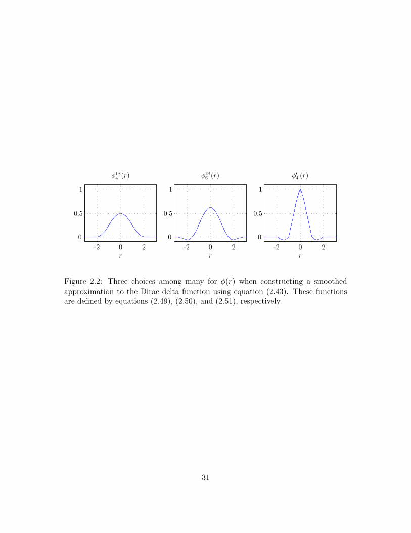
PSfrag replacements φIB4 (r)

r-2 0 2

0

0.5

1

PSfrag replacements φIB6 (r)

r-2 0 2

0

0.5

1

PSfrag replacements φC4 (r)

r-2 0 2

0

0.5

1

Figure 2.2: Three choices among many for φ(r) when constructing a smoothedapproximation to the Dirac delta function using equation (2.43). These functionsare defined by equations (2.49), (2.50), and (2.51), respectively.

31

particular choice of φ(r):

φ(r) is continuous for all real r, (2.44)

φ(r) = 0 for |r| ≥ 2, (2.45)

∑

j even

φ(r − j) =∑

j odd

φ(r − j) =1

2for all real r, (2.46)

∑

j

(r − j)φ(r − j) = 0 for all real r, and (2.47)

∑

j

(φ(r − j))2 = C for all real r, (2.48)

where the constant C is independent of r. (The construction of φ(r) from these

postulates reveals that C = 38.) A detailed motivation for these postulates is

provided in [64, 61]. The smoothed delta function that is defined in terms of the

unique function that satisfies these requirements has a support of four meshwidths

in each coordinate direction (yielding a support of 64 grid cells in three spatial

dimensions) and is referred to as the four-point delta function, which we denote by

δIB4h(x). It is is defined in terms of

φIB4 (r) =

18

(

3− 2 |r|+√

1 + 4 |r| − 4r2)

, 0 ≤ |r| < 1,

18

(

5− 2 |r| −√

−7 + 12 |r| − 4r2)

, 1 ≤ |r| < 2,

0, 2 ≤ |r| .

(2.49)

In fact, an entire family of such functions may be generated by starting with

the foregoing postulates and then imposing additional pairs of moment conditions.

32

(Note that the support of φ(r) necessarily increases as more moment conditions are

added.) By requiring the smoothed delta function to satisfy two additional discrete

moment conditions, the six-point delta function is obtained. This delta function,

first employed by Stockie [71], is denoted δIB6h(x) and is defined in terms of

φIB6 (r) =

61112− 11

42|r| − 11

56|r|2 + 1

12|r|3

+√

3336

(

243 + 1584 |r| − 748 |r|2 − 1560 |r|3

+ 500 |r|4 + 336 |r|5 − 112 |r|6)

12 ,

0 ≤ |r| < 1,

2116

+ 712|r| − 7

8|r|2 + 1

6|r|3 − 3

2φIB

6 (|r| − 1), 1 ≤ |r| < 2,

98− 23

12|r|+ 3

4|r|2 − 1

12|r|3 + 1

2φIB

6 (|r| − 2), 2 ≤ |r| < 3,

0, 3 ≤ |r| .

(2.50)

In [75], Tornberg and Engquist examine the use of smoothed delta functions in

the regularization of singular source terms in a variety of settings. One smoothed

delta function that provides them with particularly good results is the piecewise

cubic delta function, which is denoted δC4h(x) and defined in terms of

φC4 (r) =

1− 12|r| − |r|2 + 1

2|r|3 , 0 ≤ |r| < 1,

1− 116|r|+ |r|2 − 1

6|r|3 , 1 ≤ |r| < 2,

0, 2 ≤ |r| .

(2.51)

This piecewise cubic function would appear to combine the best features of the four-

point and six-point delta functions defined by (2.49) and (2.50): it has a support

of only four meshwidths and yet satisfies four moment conditions. In practice, it is

also less costly to compute than either of the other delta functions as it does not

33

require the evaluation of any square roots. However, φC4 (r) clearly cannot satisfy all

of the postulates that were used in the construction of φIB4 (r) or φIB

6 (r), and when

used with the immersed boundary method, the piecewise cubic delta function can

introduce oscillations that are suppressed by the other regularized delta functions

(especially for thin interface problems). Nonetheless, in situations where it does not

generate spurious oscillations, the piecewise cubic delta function seems to produce

results that are comparable to those obtained by using the more expensive six-point

delta function.

2.3.6 Timestepping

At the beginning of timestep n, we possess approximations to the values of the state

variables at time tn, namely un and Xn. The pressure (which is at least in principle

not a state variable) must be defined at half-timesteps to obtain a consistent second

order accurate method. Thus, at the beginning of each timestep n > 0, we also

possess an approximation to a “time-lagged” pressure, pn− 12 . We also maintain an

“auxiliary” MAC velocity, uMAC,n, that is used in our treatment of the nonlinear

advection term that appears in the momentum equation. (As we describe below,

the value of uMAC is obtained during the process of updating the cell centered

velocity, u.)

To advance the solution forward in time by the increment ∆t, we first compute

X(n+1)(q, r, s), a preliminary approximation5 to the locations of the nodes of the

5Note that X(n+1) is only our first approximation to the structure configuration at time tn+1.

The final approximation is denoted Xn+1, and generally X

(n+1) 6= Xn+1.

34

curvilinear mesh at time tn+1. To do so, equation (2.4) is approximated by

X(n+1)(q, r, s) = Xn(q, r, s) + ∆t∑

i,j,k

uni,j,k δh(xi,j,k −Xn(q, r, s)) h3. (2.52)

A discrete approximation to F [X(·, ·, ·), t] provides the curvilinear elastic force den-

sities corresponding to structure configurations Xn and X(n+1), respectively denoted

Fn and F(n+1). The equivalent Cartesian elastic force densities are obtained by dis-

cretizing (2.3) and are given by

fni,j,k =

∑

q,r,s

Fn(q, r, s) δh(xi,j,k −Xn(q, r, s)) ∆q∆r∆s, (2.53)

f(n+1)i,j,k =

∑

q,r,s

F(n+1)(q, r, s) δh(xi,j,k −X(n+1)(q, r, s)) ∆q∆r∆s. (2.54)

(In later chapters of the present work, note that we will frequently refer to such

operations as spreading the force from the curvilinear mesh to the Cartesian grid.)

A timestep-centered approximation to the Cartesian elastic force density is defined

by

fn+ 12 ≡ 1

2

(

fn + f (n+1))

. (2.55)

We next determine un+1, uMAC,n+1, and pn+ 12 by integrating the incompressible

Navier-Stokes equations in time via a second order projection method similar to

the method introduced by Bell, Colella, and Glaz [11], a method that in turn is a

second order accurate version of Chorin’s original projection method [18, 19]. Our

algorithm extends to the viscous case the hybrid approximate projection method

(“version 5”) introduced by Almgren et al. for the incompressible Euler equations

35

[3]. In particular, as in [3], we obtain the values of un+1 and pn+ 12 in terms of the

solutions to different projection equations. The value of uMAC,n+1 is obtained as a

byproduct of the computation that yields un+1.

Given un, uMAC,n, fn+ 12 , and pn− 1

2 , we first obtain the approximation to the

updated velocity, un+1. We do so by discretizing the momentum equation (2.1)

over the time interval ∆t without imposing the constraint of incompressibility on

un+1. Instead, the gradient of the time-lagged pressure provides an approximation

to the true pressure gradient. The nonlinear advection term is treated explicitly,

and a version of the implicit L-stable method of Twizell et al. [78] introduced by

McCorquodale et al. [47] is used to integrate the viscous terms in time. With

ν ≡ µ/ρ, the discretization of (2.1) is

(I − η2νL)(I − η1νL)u∗ = (2.56)

= (I + η3νL)un + ∆t(I + η4νL)

(

−Nn+ 12 +

1

ρ

(

fn+ 12 −Gpn− 1

2

)

)

,

where Nn+ 12 is the explicit approximation to [(u · ∇)u]n+ 1

2 detailed in Section 2.3.7,

and

η1 =a−√a2 − 4a+ 2

2∆t, η2 =

a+√a2 − 4a+ 2

2∆t,

η3 = (1− a) ∆t, η4 =

(

1

2− a)

∆t,

with a = 2−√

2− ε, where ε is machine precision. The derivation of this treatment

of the viscous terms is briefly outlined in Section 2.3.8.

The solution to equation (2.56) yields an “intermediate” velocity field, tradi-

36

tionally denoted u∗, that is generally not discretely divergence free. In formulating

a projection method, one may project either the velocity increment (i.e., u∗ − un)

or the intermediate velocity itself. Although either choice yields the same value for

un+1 when exact projections are employed, this is not the case when approximate

projection operators are used. Several studies have found that a more stable al-

gorithm is obtained by approximately projecting the intermediate velocity [3, 42],

and we follow this approach. In particular, un+1 is obtained by making use of the

approximate projection operator, P , defined by equation (2.32), yielding

un+1 = Pu∗. (2.57)

To compute uMAC,n+1, we first interpolate u∗ from cell centers to cell faces,

obtaining

uMAC,∗ = Ac→fu∗. (2.58)

In general, uMAC,∗ is not discretely divergence free, so uMAC,n+1 is obtained by

computing the MAC projection of uMAC,∗, i.e.,

uMAC,n+1 = PMACuMAC,∗. (2.59)

Luckily, this operation does not require the solution of an additional system of

linear equations! To see why this is so, recall that computing the approximate

projection of u∗ requires the solution of a discrete Poisson problem of the form

Lϕ = D · u∗. (2.60)

37

Since (Df→c · uMAC,∗)i,j,k ≡ (Df→c · Ac→fu∗)i,j,k ≡ (D · u∗)i,j,k, equation (2.60) is the

same linear system that must be solved to project uMAC,∗. The solution to (2.60),

ϕ, may simply be reused to evaluate

uMAC,n+1 = uMAC,∗ −Gc→fϕ. (2.61)

Having obtained the values of un+1 and uMAC,n+1, we now turn our attention

to computing the updated pressure. Although it is possible to determine this value

in terms of the approximate projection of u∗, we have found that it is beneficial

to determine pn+ 12 by approximately projecting a second intermediate velocity field

that is given by a second treatment of the momentum equation. This alternate

treatment of (2.1) is nearly identical to (2.56) except that it does not include any

approximation to the pressure gradient, i.e.,

(I − η2νL)(I − η1νL)u∗ = (2.62)

= (I + η3νL)un + ∆t(I + η4νL)

(

−Nn+ 12 +

1

ρfn+ 1

2

)

.

The solution to this equation, u∗, is the intermediate velocity that we project to

obtain pn+ 12 . We emphasize that u∗ is only used to compute pn+ 1

2 and is not used in

determining our final approximation to the velocity at time tn+1. The approximate

projection of u∗, however, generates an alternate approximation to the velocity at

time tn+1,

un+1 = P u∗ = u∗ −Gϕ, (2.63)

38

i.e.,

u∗ = un+1 + Gϕ, (2.64)

where ϕ is defined as the solution to a discrete Poisson problem,

Lϕ = D · u∗. (2.65)

Since P is an approximate projection operator, in general un+1 6= un+1.

The pressure consistent with (2.62) and (2.63) is the scalar function pn+ 12 that

satisfies

(I − η2νL)(I − η1νL)un+1 = (2.66)

= (I + η3νL)un + ∆t(I + η4νL)

(

−Nn+ 12 +

1

ρ

(

fn+ 12 −Gpn+ 1

2

)

)

.

Following [16], a second order accurate approximation to the updated pressure is

determined by substituting (2.63) back into (2.62) and comparing the result to

(2.66). Doing so, the discrete pressure gradient is seen to satisfy

(I + η4νL)Gpn+ 12 =

ρ

∆t(I − η2νL)(I − η1νL)Gϕ. (2.67)

Consequently, we obtain pn+ 12 via

pn+ 12 =

ρ

∆t(I + η4νL)−1(I − η2νL)(I − η1νL)ϕ. (2.68)

Since η4 = (√

2 − 32

+ ε)∆t < 0, and since L is a nonpositive operator, pn+ 12

39

is well-defined by (2.68). Note that ϕ is proportional to a first order accurate

approximation to the time centered pressure. Full second order accuracy is obtained

by solving a system of linear equations in (2.68). Although pn+ 12 has no influence

on the value obtained for un+1, it is used in the next timestep, when computing

un+2.

(Note that in the foregoing, equations (2.63), (2.64), (2.66), and (2.67), along

with the quantity un+1 that appears in those equations, are used to derive the

appropriate definition for the updated pressure but not to compute the value of

pn+ 12 . In particular, pn+ 1

2 is computed only in terms of u∗ and ϕ via equations

(2.62), (2.65), and (2.68).)

Having obtained the values un+1, uMAC,n+1, and pn+ 12 , we complete the timestep

by computing Xn+1 via

Xn+1(q, r, s) = Xn(q, r, s) (2.69)

+∆t

2

(

∑

i,j,k

uni,j,k δh(xi,j,k −Xn(q, r, s)) h3 +

∑

i,j,k

un+1i,j,k δh(xi,j,k −X(n+1)(q, r, s)) h3

)

Note that the evolution of the structure configuration via (2.52) and (2.69) takes the

form of a second order accurate strong stability-preserving Runge-Kutta method

[28]. Equation (2.69) is an explicit formula for Xn+1, since X(n+1) is already defined;

see equation (2.52).

Finally, we must discuss the initial timestep. The initial state of the system is

completely determined by the initial values of u and X. First, uMAC is initialized

40

by interpolating the initial value of u from cell centers to cell faces,

uMAC,0 = Ac→fu0. (2.70)

To ensure that the initial velocity at least approximately satisfies (D · u)0i,j,k ≡ 0,

we then perform an initial approximate projection, replacing u0 by

u0 ← Pu0. (2.71)

We similarly replace uMAC,0 by its MAC projection,

uMAC,0 ← PMACuMAC,0. (2.72)

Again, having computed the approximate projection of u0, it is not necessary to

solve any additional systems of linear equations to compute this initial MAC pro-

jection.

Next, the pressure must be determined from the values of u0, uMAC,0, and X0.

We obtain the pressure iteratively as follows. First, the pressure is provisionally set

to be identically zero. We then perform a preliminary timestep. The computation

of this preliminary timestep yields a first approximation to the pressure at time

t = 12∆t0. We then iteratively recompute the initial timestep, always using the

most recent approximation to the pressure. After a small number of iterations (we

use a total of five), we obtain a sufficiently accurate approximation to the pressure

at time t = 12∆t0 to achieve overall second order accuracy.

41

2.3.7 An explicit second order Godunov method

The explicit second order Godunov method that we employ to treat the nonlinear

advection terms appearing in the incompressible Navier-Stokes equations is based

on well-established methods introduced by Colella for the advection equation and

hyperbolic conservation laws [20], methods that were first applied to the incom-

pressible Navier-Stokes equations by Bell, Colella, and Glaz [11]. The particular

methodology that we employ combines versions of the original scheme that have

been further specialized to the case of incompressible flow by Minion [54, 55] and

Martin and Colella [42]. The purpose of the present section is simply to document

the particular choices that we have made for the convenience of the reader.

Note that in the present subsection, variables affixed with a “∼” are generally

different from the quantities u∗, un+1, and ϕ defined in Section 2.3.6.

An explicit Godunov extrapolation procedure

To simplify the description of the Godunov procedure, we temporarily restrict our

attention in this section to the advection-diffusion equation,

∂c

∂t+ (u · ∇)c = ν∇2c+ ψ, (2.73)

where c is a scalar quantity that is being advected and diffused, u is a specified

advection velocity, ν ≥ 0 is the diffusion coefficient, and ψ is a given source term.

Our goal in this section is to describe an explicit second order accurate procedure

that uses values defined at time tn to extrapolate the face centered value of c at time

tn+ 12. Although described only for the advection-diffusion equation, the following

42

procedure is used without modification as part of our approximation to the nonlinear

advection term appearing in the incompressible Navier-Stokes equations.

The particular procedure that we employ is an explicit Godunov method intro-

duced by Colella for the advection equation [20], and modified by Minion in the case

that c is being both advected and diffused [54]. The idea is to extrapolate c from

cell centers to cell faces by using Taylor expansions for c about the Cartesian grid

cell centers. Notice that this extrapolation process is ambiguous: at every cell face,

there are two nearest cell centers and hence two Taylor expansions to choose from.

The ambiguity is resolved by using the expansion that is about the cell center that

lies in the upwind direction—a method motivated by the solution to the Riemann

problem for the one-dimensional Burgers’ equation.

In order to obtain a stable explicit extrapolation scheme, the timestep must

satisfy a condition of the form ∆t = O(h). Consequently, the Taylor series for

c(x, t), taken about the point xi,j,k and evaluated at cell face xi+ 12,j,k and at time

t = tn+ 12, is

cn+ 1

2,L

i+ 12,j,k

= cni,j,k +h

2(cx)

ni,j,k +

∆t

2(ct)

ni,j,k +O(h2). (2.74)

Note that in this expansion, the face centered value of c is obtained in terms of cell

centered quantities that lie to the left of cell face xi+ 12,j,k. The time derivative, ct,

43

can be eliminated by making use of equation (2.73), yielding

cn+ 1

2,L

i+ 12,j,k

= cni,j,k +

(

h

2− ∆t

2un

i,j,k

)

(cx)ni,j,k (2.75)

− ∆t

2

(

vni,j,k

(

∂

∂y

(

c− ∆t

3wcz

))n

i,j,k

+ wni,j,k

(

∂

∂z

(

c− ∆t

3vcy

))n

i,j,k

)

+∆t

2

(

ν(∇2c)ni,j,k + ψn

i,j,k

)

+O(h2),

where u = (u, v, w). A similar expansion about xi+1,j,k, evaluated at face xi+ 12,j,k,

yields the right state,

cn+ 1

2,R

i+ 12,j,k

= cni+1,j,k −(

h

2+

∆t

2un

i+1,j,k

)

(cx)ni+1,j,k (2.76)

− ∆t

2

(

vni+1,j,k

(

∂

∂y

(

c− ∆t

3wcz

))n

i+1,j,k

+ wni+1,j,k

(

∂

∂z

(

c− ∆t

3vcy

))n

i+1,j,k

)

+∆t

2

(

ν(∇2c)ni+1,j,k + ψn

i+1,j,k))

+O(h2).

Similar expansions define the front and back states, cn+ 1

2,F/B

i,j+ 12,k

, as well as the down

and up states, cn+ 1

2,D/U

i,j,k+ 12

. Notice that the foregoing Taylor expansions include both

the terms required to obtain second order accuracy as well as the higher order terms

required for full corner transport coupling in three spatial dimensions [68].

Following [54, 55], a second order approximation to each of the proceeding

Taylor expansions is computed in two steps. The resulting scheme is stable so long

as the timestep satisfies a CFL condition of the form ‖u‖∞∆t ≤ h, independent of

the value of ν ≥ 0. Though capital letters are generally reserved for Lagrangian

variables in the remainder of this work, in the following expressions it is convenient

44

to let Uni,j,k = (Un

i,j,k, Vni,j,k,W

ni,j,k) denote a cell centered velocity field defined on the

Cartesian grid that is determined by Un = Af→cuMAC,n.

In the first step of the scheme, cn+ 1

2,F

i,j+ 12,k

is approximated by

cn+ 1

2,F

i,j+ 12,k

= cni,j,k +1

2

(

1− ∆t

hV n

i,j,k

)

(

D0yc)n

i,j,k+

∆t

2

(

ν(Lc)ni,j,k + ψn

i,j,k

)

, (2.77)

where D0y is a fourth order centered difference operator defined by

(

D0yc)n

i,j,k=

2

3

(

cni,j+1,k − cni,j−1,k

)

− 1

12

(

cni,j+2,k − cni,j−2,k

)

. (2.78)

Similarly, cn+ 1

2,B

i,j+ 12,k

is approximated by

cn+ 1

2,B

i,j+ 12,k

= (2.79)

= cni,j+1,k −1

2

(

1 +∆t

hV n

i,j+1,k

)

(

D0yc)n

i,j+1,k+

∆t

2

(

ν(Lc)ni,j+1,k + ψn

i,j+1,k

)

.

Analogous approximations define cn+ 1

2,L/R

i+ 12,j,k

and cn+ 1

2,D/U

i,j,k+ 12

. Note that each of these

values includes approximations only to those derivative terms that are normal to the

cell face where the expansion is being approximated. For now, transverse derivatives

(i.e., derivatives in directions that are tangential to a face) are not included.

At each cell face, cn+ 12 is defined by choosing the upwind state, for instance

cn+ 1

2

i,j,k+ 12

=

cn+ 1

2,D

i,j,k+ 12

, if uMAC,n

i,j,k+ 12

> 0,

cn+ 1

2,U

i,j,k+ 12

, if uMAC,n

i,j,k+ 12

< 0,

12

(

cn+ 1

2,D

i,j,k+ 12

+ cn+ 1

2,U

i,j,k+ 12

)

, if uMAC,n

i,j,k+ 12

= 0,

(2.80)

45

and similarly for cn+ 1

2

i+ 12,j,k

and cn+ 1

2

i,j+ 12,k.

The second step in the extrapolation procedure introduces approximations to

the transverse derivative terms. These approximations are obtained by differencing

the initial extrapolation, cn+ 12 . In particular, we have

cn+ 1

2,L

i+ 12,j,k

= cn+ 1

2

i+ 12,j,k− ∆t

2hV n

i,j,k

(

cn+ 1

2

i,j+ 12,k− cn+ 1

2

i,j− 12,k

)

− ∆t2hW n

i,j,k

(

cn+ 1

2

i,j,k+ 12

− cn+ 12

i,j,k− 12

)

+ ∆t2

6h2 Vni,j,k×

(

W ni,j,k

(

cn+ 1

2

i,j,k+ 12

− cn+ 12

i,j,k− 12

)

−W ni,j−1,k

(

cn+ 1

2

i,j−1,k+ 12

− cn+ 12

i,j−1,k− 12

))

, if V ni,j,k > 0,

(

W ni,j+1,k

(

cn+ 1

2

i,j+1,k+ 12

− cn+ 12

i,j+1,k− 12

)

−W ni,j,k

(

cn+ 1

2

i,j,k+ 12

− cn+ 12

i,j,k− 12

))

, otherwise.

+ ∆t2

6h2Wni,j,k×

(

V ni,j,k

(

cn+ 1

2

i,j+ 12,k− cn+ 1

2

i,j− 12,k

)

− V ni,j,k−1

(

cn+ 1

2

i,j+ 12,k−1− cn+ 1

2

i,j− 12,k−1

))

, if W ni,j,k > 0,

(

V ni,j,k+1

(

cn+ 1

2

i,j+ 12,k+1− cn+ 1

2

i,j− 12,k+1

)

− V ni,j,k

(

cn+ 1

2

i,j+ 12,k− cn+ 1

2

i,j− 12,k

))

, otherwise.

where here we have included approximations to the remaining terms required to

obtain second order accuracy and to the terms required for full corner coupling

in three spatial dimensions. Similar formulas yield the remaining values. Finally,

having determined cn+ 1

2,L/R

i+ 12,j,k

, cn+ 1

2,F/B

i,j+ 12,k

, and cn+ 1

2,D/U

i,j,k+ 12

, the value of cn+ 12 is obtained

on each cell face by choosing the upwind state as in (2.80).

Note that the inclusion of the higher order terms that yield full corner coupling

in three spatial dimensions does not increase the formal order of accuracy of the

scheme. Excluding them would still yield a second order accurate method and

would incur only a modest reduction in the size of the largest stable timestep. In

46

practice, however, including these additional terms yields an insignificant increase

in the overall cost of the present version of the immersed boundary method, and so

we include these terms in the hope that full corner coupling increases the quality

of the solution.

Computing the advection term

In order to compute the explicit approximation to the nonlinear advection term,

[(u · ∇)u]n+ 12 , used in the solution of the incompressible Navier-Stokes equations,

we employ a timestep centered advection velocity, denoted uADV. This advection

velocity is a discretely divergence free MAC vector field and is obtained in two

steps:

The first step in obtaining uADV employs the previously detailed Godunov

scheme to extrapolate to the cell faces each component of the cell centered velocity,

uni,j,k = (un

i,j,k, vni,j,k, w

ni,j,k). This is performed component-wise, i.e., we first employ

the Godunov procedure with uni,j,k replacing cni,j,k and employ the corresponding

source term,

ψni,j,k =

1

ρ

(

(f1)ni,j,k − (Gxp)

n− 12

i,j,k

)

, (2.81)

where f = (f1, f2, f3) is the discrete Cartesian elastic force density and Gp =

(Gxp,Gyp,Gzp) is the discrete pressure gradient. This yields a timestep centered

approximation to u at each cell face in the Cartesian grid. The analogous procedure

is performed for v and w, ultimately yielding timestep centered approximations to

u, v, and w at each cell face in the grid. These extrapolated velocities are denoted

un+ 12 , vn+ 1

2 , and wn+ 12 .

47

The second step in obtaining uADV discards the transverse components of the

extrapolated velocity field (i.e., velocities in directions that are tangential to a

face). This yields a MAC velocity, denoted uADV,∗, that generally is not discretely

divergence free with respect to Df→c·, the MAC divergence operator. To enforce

incompressibility, the advection velocity is defined to be the MAC projection of

uADV,∗, i.e.,

uADV = PMACuADV,∗ = uADV,∗ −Gc→fϕADV, (2.82)

where ϕADV is the solution to a discrete Poisson problem,

LϕADV = Df→c · uADV,∗. (2.83)

This completes the procedure for computing uADV.

With uADV in hand, we next re-extrapolate the timestep centered normal and

transverse velocities at each cell face, using the timestep centered advection velocity,

uADV, in place of uMAC,n. Except for this one difference, the extrapolation procedure

is identical to that previously used to obtain un+ 12 , vn+ 1

2 , and wn+ 12 . Doing so yields

a second approximation to the timestep centered normal and transverse velocities

at each cell face in the Cartesian grid, denoted un+ 12 , vn+ 1

2 , and wn+ 12 . (Note that

we do not discard the transverse components of the re-extrapolated velocity field.)

Next, the solution to (2.83), ϕADV, is used to approximately enforce the incom-

pressibility constraint. For the velocities that are normal to the cell face where they

48

are defined, we set

un+ 1

2

i+ 12,j,k

= un+ 1

2

i+ 12,j,k− 1

h

(

ϕADVi+1,j,k − ϕADV

i,j,k

)

, (2.84)

vn+ 1

2

i,j+ 12,k

= vn+ 1

2

i,j+ 12,k− 1

h

(

ϕADVi,j+1,k − ϕADV

i,j,k

)

, (2.85)

wn+ 1

2

i,j,k+ 12

= wn+ 1

2

i,j,k+ 12

− 1

h

(

ϕADVi,j,k+1 − ϕADV

i,j,k

)

, (2.86)

whereas for the transverse components, we have, for instance,

un+ 1

2

i,j+ 12,k

= un+ 1

2

i,j+ 12,k− 1

4h

(

ϕADVi+1,j,k − ϕADV

i−1,j,k + ϕADVi+1,j+1,k − ϕADV

i−1,j+1,k

)

, (2.87)

vn+ 1

2

i,j,k+ 12

= vn+ 1

2

i,j,k+ 12

− 1

4h

(

ϕADVi,j+1,k − ϕADV

i,j−1,k + ϕADVi,j+1,k+1 − ϕADV

i,j−1,k+1

)

, (2.88)

wn+ 1

2

i+ 12,j,k

= wn+ 1

2

i+ 12,j,k− 1

4h

(

ϕADVi,j,k+1 − ϕADV

i,j,k−1 + ϕADVi+1,j,k+1 − ϕADV

i+1,j,k−1

)

, (2.89)

and similarly for the remaining transverse components. Note that in each case, the

appropriate component of a discrete gradient of ϕADV is being used to approximately

enforce the incompressibility constraint6.

At long last, the approximation to the nonlinear advection term,

Nn+ 1

2i,j,k =

(

(N1)n+ 1

2i,j,k , (N2)

n+ 12

i,j,k , (N3)n+ 1

2i,j,k

)

≈ [(u · ∇)u]n+ 1

2i,j,k , (2.90)

6This “pseudo-projection” may strike the reader as a peculiar thing to do; however, doing soyields a modest reduction in the errors in the computed solutions obtained by the approximateprojection method when it is tested against known exact solutions to the incompressible Navier-Stokes equations. Similar approaches are employed in the approximate projection methods of,e.g., [3, 42].

49

is defined by non-conservative differencing where, for instance,

(N1)n+ 1

2i,j,k =

1

2h

(

uADVi+ 1

2,j,k

+ uADVi− 1

2,j,k

) (

un+ 1

2

i+ 12,j,k− un+ 1

2

i− 12,j,k

)

(2.91)

+1

2h

(

vADVi,j+ 1

2,k

+ vADVi,j− 1

2,k

) (

un+ 1

2

i,j+ 12,k− un+ 1

2

i,j− 12,k

)

+1

2h

(

wADVi,j,k+ 1

2+ wADV

i,j,k− 12

)(

un+ 1

2

i,j,k+ 12

− un+ 12

i,j,k− 12

)

,

with N2 and N3 defined similarly. Since uADV is discretely divergence free, we could

have employed conservative differencing here to approximate the advection term.

We do not do so, however, as we find that the use of non-conservative differencing

produces lower errors when we test the approximate projection method against

known analytic solutions to the incompressible Navier-Stokes equations.

2.3.8 An L-stable scheme for linear parabolic problems

In Section 2.3.6, a version of the implicit L-stable method of Twizell et al. [78]

introduced by McCorquodale et al. [47] is employed for the time integration of the

viscous terms in equations (2.56) and (2.62). L-stability, which is defined shortly,

is a strengthened version of the more familiar notion of A-stability. Before defining

L-stability, we motivate the method by considering a semi-discretization of a linear

parabolic equation with a time-dependent source term, namely

du

dt(xi,j,k, t) = (Lu)(xi,j,k, t) + f(xi,j,k, t), (2.92)

u(xi,j,k, 0) = g(xi,j,k). (2.93)

50

Restricting our attention temporarily to the case f ≡ 0, the exact solution to (2.92)

and (2.93) is given for t = t0, t1, t2, . . . , by the recurrence relation

u(xi,j,k, tn+1) = (exp(∆tL)u)(xi,j,k, tn), (2.94)

where ∆t = tn+1 − tn.

Following [78], let R(∆tL) denote an approximation to exp(∆tL) of the form

R(∆tL) = (I − a∆tL + b∆t2L2)−1[I + (1− a)∆tL], (2.95)

where a and b are presently undetermined parameters of the method. The approx-

imation to the exact solution is denoted uni,j,k and satisfies the recurrence

un+1i,j,k = (R(∆tL)u)n

i,j,k. (2.96)

The order of accuracy of the method and its stability properties can be deter-

mined by applying the scheme to the simple scalar equation

dy

dt(t) = λy(t), (2.97)

where Re(λ) < 0. One can determine that the local truncation error of the method

is given by

y(tn)− yn =

(

1

2− a+ b

)

∆t2 y′′(tn) +

(

1

6− a

2+ b

)

∆t3 y′′′(tn) +O(∆t4). (2.98)

51

Consequently, to obtain a second order accurate method it is necessary that

b = a− 1

2. (2.99)

A discretization of (2.97) said to be A-stable if for any initial value, y0, and for

any ∆t > 0, yn decays to zero as n → ∞. An A-stable method for (2.97) is

said to be L-stable if for any value of yn, yn+1 tends to zero as ∆t → ∞. Since

yn+1 = R(∆tλ)yn, where (recalling equations (2.95) and (2.99))

R(∆tλ) =1 + (1− a)∆tλ

1− a∆tλ +(

a− 12

)

∆t2λ2, (2.100)

one can show the scheme is L-stable so long as

a >1

2. (2.101)

Note that setting a = 12

yields the trapezoidal rule, a method that is A-stable but

not L-stable. The trapezoidal rule fails to be L-stable since given any value of yn,

yn+1 → −yn as ∆t→∞.

To implement the scheme using fast linear solvers, it is helpful to factor the

denominator of equation (2.95), with a 6= 12, to obtain

R(∆tL) = (I − η1L)−1(I − η2L)−1[I + η3L], (2.102)

with η1 = a−√

a2−4a+22

∆t, η2 = a+√

a2−4a+22

∆t, and η3 = (1− a) ∆t. If η1 6= η2, a

52

partial fractions decomposition of (2.102) can be obtained, namely

R(∆tL) =1− a + η1

η1 − η2(I − η1L)−1 +

1− a+ η2

η2 − η1(I − η2L)−1. (2.103)

Complex coefficients are avoided in (2.102) and (2.103) for a2 − 4a+ 2 ≥ 0. To

additionally obtain η1 6= η2, we require a to satisfy the stronger condition

a < 2−√

2 or a > 2 +√

2. (2.104)

Subject to (2.104), theO(∆t3) term in (2.98) is approximately minimized in floating

point arithmetic by setting a = 2−√

2− ε, where ε is machine precision. Since this

choice of a satisfies (2.101), in this case the method is also L-stable. Note that this

is the value of a used in Section 2.3.6, although presently we do not make use of

the partial fractions decomposition, (2.103).

For f 6≡ 0, we follow McCorquodale et al. [47] and set

un+1i,j,k = (R(∆tL)u)n

i,j,k + ∆t(S(∆tL)f)n+ 1

2i,j,k , (2.105)

where

S(∆tL) = (I − η1L)−1(I − η2L)−1[I + η4∆tL], (2.106)

where η1 and η2 are as given above and η4 =(

12− a)

∆t.

53

2.4 The adaptive discretization of the equations

of motion

The present section extends the foregoing uniform grid method to provide an adap-

tive discretization of the Eulerian equations of motion (i.e., the incompressible

Navier-Stokes equations). In particular, we replace the uniform Cartesian grid

discretization of the physical domain, U , with a hierarchy of nested grids with suc-

cessively finer mesh spacings. Although approximate projection methods for the

incompressible Euler [42] and Navier-Stokes [2] equations have been developed for

such locally refined grids that perform local refinement in time as well as in space, in

the present work all levels of the grid hierarchy are advanced synchronously, thereby

simplifying both the description of the adaptive method and its implementation.

As in the non-adaptive method, the discretization of the curvilinear coordinate

space is fixed, but it is important to emphasize again that the physical locations

of the nodes of the curvilinear mesh, Xn(q, r, s), are free to move throughout the

physical domain and are not required to conform to the Cartesian grid. By contrast,

in the present scheme, the Cartesian grid is required to conform to the evolving

configuration of the curvilinear mesh since we adaptively deploy local refinement

in the vicinity of the elastic structure.

2.4.1 Hierarchical structured Cartesian grids

The locally refined Cartesian grid is composed of the union of rectangular grid

patches that are organized into a sequence of patch levels (see Figure 2.3). We shall

54

frequently refer to the collection of patch levels as the patch hierarchy, or simply

the hierarchy. The levels are numbered ` = 0, . . . , `max, where ` = 0 indicates the

coarsest level in the hierarchy and ` = `max indicates the finest level. All of the

patches in level ` share the same grid spacings, (∆x`,∆y`,∆z`), although for the

purposes of the present discussion it suffices to assume that h` = ∆x` = ∆y` = ∆z`.

The grid spacing on a particular level is not arbitrary; instead, the grid spacing at

level `+1 is required to be an integer factor r > 1 finer than the grid spacing at level

`, so that h`+1 = h`/r. Although typical choices for this refinement ratio are r = 2

or 4, in the present scheme any integer r > 1 may be employed as the refinement

ratio. (In fact, in the implementation of the adaptive method, the refinement ratio

is neither fixed across the entire patch hierarchy nor required to be isotropic. These

slight generalizations of the presented method are easily implemented in practice

but do not seem sufficiently important to warrant the additional notation required

by their description.) As in the uniform grid method, the centers of the Cartesian

grid cells on level ` are the points xi,j,k =(

(i + 12)h`, (j + 1

2)h`, (k + 1

2)h`

)

, although

it is important to note that in general only patch level 0 completely covers the

physical domain. Thus, on a locally refined grid, the level ` grid cells are a subset of

the cells of a uniform discretization of the physical domain with the same resolution

as level `.

The patch levels are required to be properly nested in the sense that the union

of the grid patches at level ` + 1 must be strictly contained in the union of the

patches at level `. That is, the union of the level ` patches must be large enough

to provide at least a one cell wide buffer of unrefined level ` grid cells around the

union of the level ` + 1 patches. Note that this is not equivalent to requiring

55

PSfrag replacements

Level 0

Level 1

Level 2

Figure 2.3: A properly nested hierarchical structured locally refined Cartesian grid.Patch boundaries are indicated by bold lines. Each level in the patch hierarchyconsists of one or more rectangular grid patches, and the levels satisfy the propernesting condition. Here, the refinement ratio is r = 2. (Compare to the improperlynested configuration of Figure 2.4.)

56

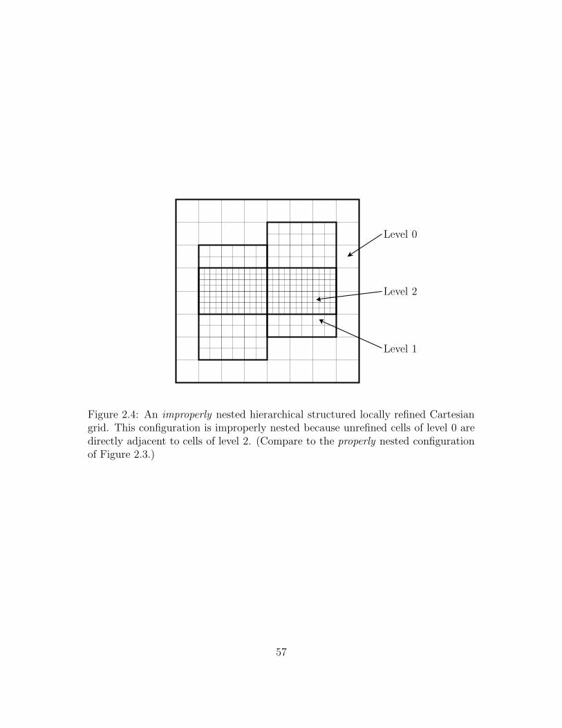
PSfrag replacements

Level 0

Level 1

Level 2

Figure 2.4: An improperly nested hierarchical structured locally refined Cartesiangrid. This configuration is improperly nested because unrefined cells of level 0 aredirectly adjacent to cells of level 2. (Compare to the properly nested configurationof Figure 2.3.)

57

that each level ` + 1 patch be contained (strictly or otherwise) within a single

level ` patch. The nesting requirement is typically relaxed at domain boundaries

with prescribed physical boundary conditions (but not at periodic boundaries).

Figure 2.3 displays a locally refined grid that satisfies the proper nesting condition,

whereas Figure 2.4 demonstrates how a locally refined grid may fail to satisfy the

proper nesting condition.

The patch hierarchy is constructed, either at the initial time or at a later point in

the computation (i.e., during adaptive regridding), by a simple recursive procedure,

as follows. The coarsest level, namely level 0, consists of one or more grid patches

whose union completely covers the physical domain, U . Next, having constructed

levels 0, . . . , ` < `max, grid cells at level ` are tagged for further refinement according

to criteria described below, thereby identifying the portion of level ` that requires

still higher spatial resolution. These tagged cells are grouped together into rectan-

gular grid patches by a parallel implementation of the Berger-Rigoutsos clustering

algorithm [14] described by Wissink et al. [80]. The level ` boxes generated by the

clustering algorithm are subsequently refined by the refinement ratio, r, to form

the new level ` + 1 patches. (Note that a consequence of this construction is that

fine level `+ 1 grid patch boundaries align with coarse level ` grid cell boundaries.

This property simplifies interlevel data communication as well as the development

of numerical methods on the locally refined grid.) This process is repeated until

the specified maximum number of levels have been generated. Along the way, care

must be taken to ensure that the patch levels satisfy the proper nesting condition.

It may also be necessary to further modify the generated boxes to achieve good load

balancing and communications efficiency in parallel computational environments,

58

but further discussion of such details is postponed to Chapter 3.

During the initial construction and subsequent regriddings of the patch hier-

archy, grid cells are tagged for refinement when they contain one or more curvi-

linear mesh nodes. More precisely, cell (i, j, k) on level ` < `max is tagged for

refinement if there exists a curvilinear mesh node (q, r, s) such that Xn(q, r, s) ∈

[ih`, (i+ 1)h`) × [jh`, (j + 1)h`) × [kh`, (k + 1)h`). A consequence of this tagging

criteria is that the elastic structure is embedded in the finest level of the patch hi-

erarchy. (A generalization that we do not consider here is to assign portions of the

elastic structure to levels other than the finest one.) Additional grid cells are tagged

for refinement on level `max − 1 both to prevent the structure from “escaping” the

finest level of the patch hierarchy between regridding operations, and to ensure that

the structure configuration is sufficiently far from the coarse-fine interface between

levels `max− 1 and `max to avoid complicating the discretization of the Lagrangian-

Eulerian interaction equations. In particular, when velocity interpolation and force

spreading are performed via a regularized delta function with a support of d mesh-

widths in each coordinate direction, we ensure that the physical position of each

node of the curvilinear mesh is at least dd/2e+ 1 grid cells away from the nearest

coarse-fine interface on level `max. Additional cells may be tagged for refinement

according to feature detection criteria (e.g., based on the local magnitude of the

vorticity) or other user-defined error estimators.

Each grid cell at level ` < `max either is completely covered by cells on the next

finer level or is not refined at all. Analogously, each cell face either is completely

covered by cell faces on the next finer level or is not refined at all. Since we assume

that the solution on finer levels is more accurate than that on coarser levels, we

59

distinguish between valid and invalid regions of each level. For a cell centered

quantity, the valid region of level ` consists of precisely those level ` cells that are

not covered by any finer grid cells. Similarly, for a face centered quantity, the valid

region of level ` consists of those level ` grid faces that are not covered by any

finer faces. Note that face centered quantities defined on the coarse-fine interface

between levels ` and ` + 1 are valid on level `+ 1 but not on level `.

In the present scheme, all quantities defined on the locally refined Cartesian grid

are considered composite grid variables. For such a variable, the degrees of freedom

are precisely those values that are within the valid region of each level of the patch

hierarchy. The values in the invalid region of each level are implicitly defined in

terms of the underlying fine grid values. In particular, values of a composite grid

variable in the invalid region of level ` < `max are defined to be the conservative

averages of the underlying fine grid values on level `+ 1. Note that this definition

for the values in the invalid region has a recursive character, since it is possible

that an invalid grid cell at level ` may be covered not only by cells on level ` + 1

but also by cells from finer levels. We make use of both cell centered composite

grid variables and face centered composite grid variables (including composite grid

MAC vector fields) in the adaptive scheme.

Although we do not make use of them in the description of the adaptive dis-

cretization, we shall additionally make use of level variables in Chapter 3 when

we discuss the parallel linear solvers that are employed in the implementation of

the adaptive scheme. Unlike composite grid variables, the degrees of freedom for

a level variable include values in both the valid and invalid regions of each patch

level. In particular, the values of a level variable in the invalid region of a level are

60

not assumed to be related in any way to values defined on other patch levels.

2.4.2 Interpolation and finite difference operators on lo-

cally refined grids

We now turn our attention to the modifications to the interpolation and finite dif-

ference operators introduced in Section 2.3.2 that are necessitated by the presence

of local grid refinement. One of the benefits of the structured local mesh refinement

approach is that uniform grid discretizations generally may be employed without

modification away from coarse-fine interfaces between levels of refinement. As we

describe presently, in some cases it is possible to use essentially unmodified uniform

grid interpolation or difference operators throughout each level of the patch hierar-

chy, whereas in other cases it is necessary to modify the interpolation and difference

stencils at coarse-fine interfaces. In particular, we use the requirement that values

in the invalid region of a patch level be defined as the conservative averages of the

underlying fine grid data to show that Af→c and Df→c· may be used essentially

without modification at coarse-fine interfaces. On the other hand, it is necessary to

modify the definitions of Ac→f and Gc→f at coarse-fine interfaces. (Recall that we

use these “c→ f” and “f→ c” operators to define the purely cell centered difference

operators, namely G, D·, and L.)

In an attempt to simplify the discussion, we first consider the discretizations

at the coarse-fine interface on a two-dimensional grid before considering the more

complicated three-dimensional cases. In particular, we consider a portion of the

interface between levels `− 1 and ` where a coarse cell, denoted (I − 1, J), lies di-

61

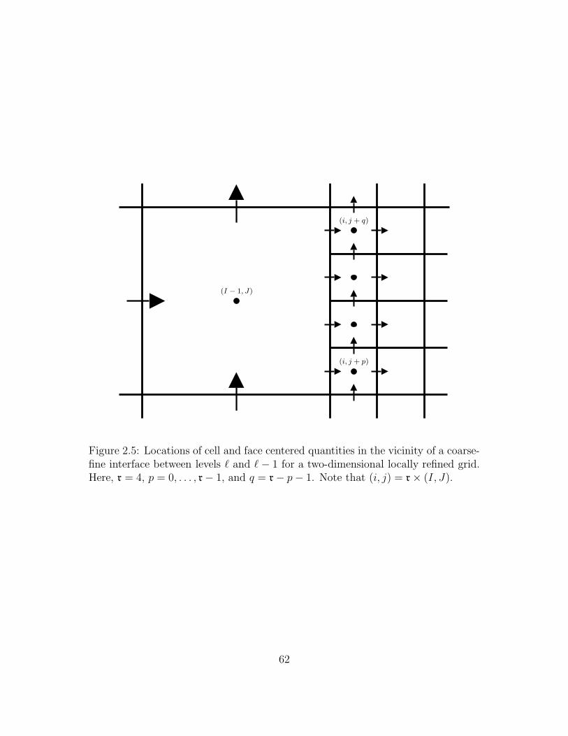
PSfrag replacements

(I − 1, J)

(i, j + p)

(i, j + q)

Figure 2.5: Locations of cell and face centered quantities in the vicinity of a coarse-fine interface between levels ` and `− 1 for a two-dimensional locally refined grid.Here, r = 4, p = 0, . . . , r− 1, and q = r− p− 1. Note that (i, j) = r× (I, J).

62

rectly to the left of r fine cells, collectively denoted (i, j), (i, j + 1), . . . , (i, j + r− 1).

This situation is depicted in Figure 2.5. When a careful presentation of the three-

dimensional case is required, we shall consider an analogous situation for a three-

dimensional locally refined grid, where coarse cell (I−1, J,K) lies directly to the left

of r2 fine cells, (i, j, k), . . . , (i, j + r− 1, k), (i, j, k + 1), . . . , (i, j + r− 1, k + r− 1).

In the two-dimensional case, note that (i, j) = r × (I, J), and that in the three-

dimensional case, (i, j, k) = r× (I, J,K).

Composite grid definitions for Af→c and Df→c·

Recall that values in the invalid regions of each level in the patch hierarchy are

defined to be the conservative averages of the underlying fine data. To make this

more concrete, consider a scalar function u defined on the x-faces of the composite

grid. In reference to the two-dimensional configuration illustrated by Figure 2.5,

we have that the (invalid) value uI− 12,J is defined as the conservative average of the

underlying fine grid values, namely

uI− 12,J =

1

r

r−1∑

p=0

ui− 12,j+p. (2.107)

The three-dimensional case is similar, with

uI− 12,J,K =

1

r2

r−1∑

pj ,pk=0

ui− 12,j+pj,k+pk

. (2.108)

In either case, the remaining coarse grid values in the invalid region are determined

in an analogous fashion. With the values in the invalid regions of each level in

63

the patch hierarchy so defined, the composite grid definitions of the interpolation

operator Af→c and the discrete divergence operator Df→c· are obtained by employing

the uniform grid operators throughout each level of the patch hierarchy without

further modification at coarse-fine interfaces. Simple procedures for evaluating

these composite grid operators on each level of the patch hierarchy are outlined in

Algorithms 2.1 and 2.2. Note that in the case of Af→c, an additional step is required

to synchronize the interpolated values in the invalid region of each level with the

underlying fine values.

We now consider the order of accuracy of these composite grid operators in the

vicinity of a coarse-fine interface. On the “fine side” of any coarse-fine interface, it is

clear that both Af→c and Df→c· are second order accurate. Their orders of accuracy

on the “coarse side” of a coarse-fine interface may be determined by considering

the Taylor series expansions of u(x). In reference to Figure 2.5, the relevant Taylor

expansions of u(x) evaluated at coarse cell center xI−1,J are

ui− 12,j+p = uI−1,J +

rh`

2(∂xu)I−1,J +

(

p− r− 1

2

)

h` (∂yu)I−1,J +O(

h2`

)

,

uI− 32,J = uI−1,J −

rh`

2(∂xu)I−1,J +O

(

h2`

)

,

where p = 0, . . . , r − 1. When we interpolate u(x) from x-faces (I − 32, J) and

(I − 12, J) to cell center (I − 1, J) via Algorithm 2.1, we have that

(Af→c1 u)I−1,J =

1

2

(

uI− 12,J + uI− 3

2,J

)

=1

2

(

1

r

r−1∑

p=0

(

ui− 12,j+p

)

+ uI− 32,J

)

64

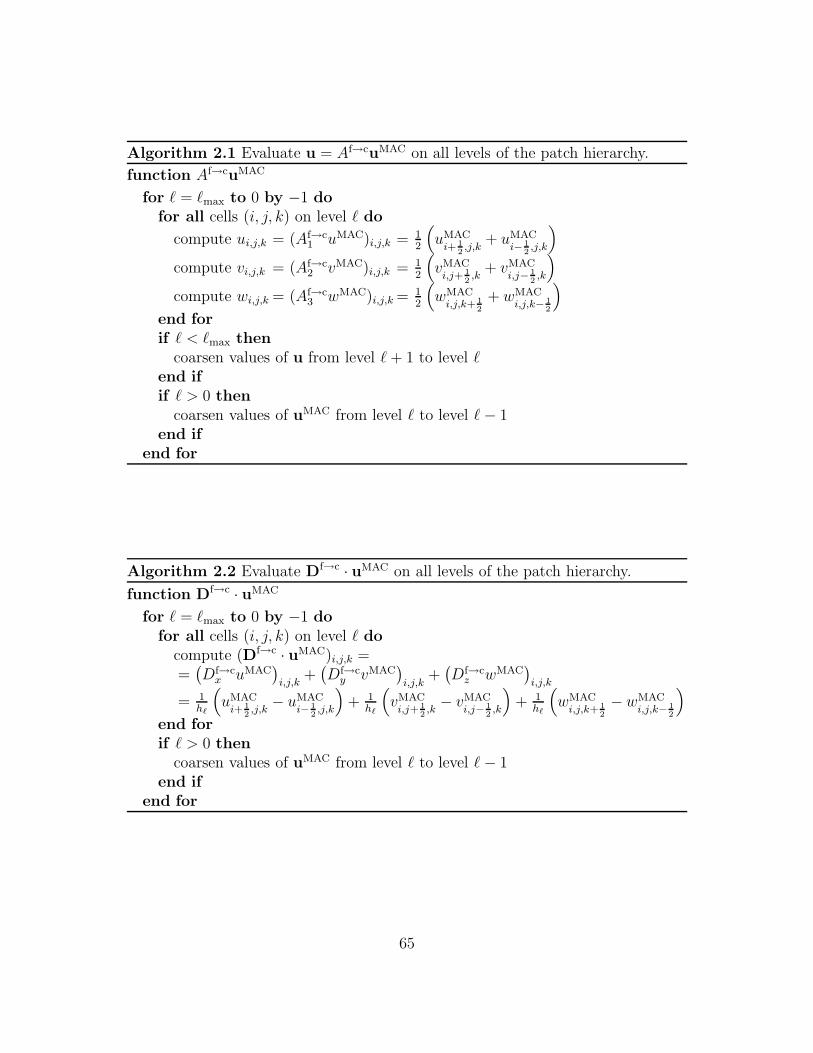
Algorithm 2.1 Evaluate u = Af→cuMAC on all levels of the patch hierarchy.

function Af→cuMAC

for ` = `max to 0 by −1 do

for all cells (i, j, k) on level ` do

compute ui,j,k = (Af→c1 uMAC)i,j,k = 1

2

(

uMACi+ 1

2,j,k

+ uMACi− 1

2,j,k

)

compute vi,j,k = (Af→c2 vMAC)i,j,k = 1

2

(

vMACi,j+ 1

2,k

+ vMACi,j− 1

2,k

)

compute wi,j,k = (Af→c3 wMAC)i,j,k = 1

2

(

wMACi,j,k+ 1

2

+ wMACi,j,k− 1

2

)

end for

if ` < `max then

coarsen values of u from level `+ 1 to level `end if

if ` > 0 then

coarsen values of uMAC from level ` to level `− 1end if

end for

Algorithm 2.2 Evaluate Df→c · uMAC on all levels of the patch hierarchy.

function Df→c · uMAC

for ` = `max to 0 by −1 do

for all cells (i, j, k) on level ` do

compute (Df→c · uMAC)i,j,k ==(

Df→cx uMAC

)

i,j,k+(

Df→cy vMAC

)

i,j,k+(

Df→cz wMAC

)

i,j,k

= 1h`

(

uMACi+ 1

2,j,k− uMAC

i− 12,j,k

)

+ 1h`

(

vMACi,j+ 1

2,k− vMAC

i,j− 12,k

)

+ 1h`

(

wMACi,j,k+ 1

2

− wMACi,j,k− 1

2

)

end for

if ` > 0 then

coarsen values of uMAC from level ` to level `− 1end if

end for

65

by equation (2.107). Making use of the Taylor expansions yields

(Af→c1 u)I−1,J =

1

2

(

1

r

r−1∑

p=0

(

uI−1,J +rh`

2(∂xu)I−1,J +

(

p− r− 1

2

)

h` (∂yu)I−1,J

)

+ uI−1,J −rh`

2(∂xu)I−1,J +O

(

h2`

)

)

= uI−1,J +1

2

(

1

r

r−1∑

p=0

(

p− r− 1

2

)

h` (∂yu)I−1,J

)

+O(

h2`

)

= uI−1,J +O(

h2`

)

sincer−1∑

p=0

(

p− r− 1

2

)

= −r(r− 1)

2+

r−1∑

p=0

p = 0.

Thus, Af→c is second order accurate on both sides of the coarse-fine interface de-

picted in Figure 2.5. Similar calculations demonstrate that Af→c is second order

accurate for all possible coarse-fine interface orientations for both two-dimensional

and three-dimensional locally refined grids.

Similarly, when we compute the cell centered difference of u(x) at cell (I−1, J)

from its values at cell faces (I − 32, J) and (I − 1

2, J) via Algorithm 2.2, we have

that

(Df→cx u)I−1,J =

1

rh`

(

uI− 12,J − uI− 3

2,J

)

=1

rh`

(

1

r

r−1∑

p=0

(

ui− 12,j+p

)

− uI− 32,J

)

,

66

again by equation (2.107). Making use of the Taylor expansions, we see that

(Df→cx u)I−1,J =

1

rh`

(

1

r

r−1∑

p=0

(

uI−1,J +rh`

2(∂xu)I−1,J +

(

p− r− 1

2

)

h` (∂yu)I−1,J

)

− uI−1,J +rh`

2(∂xu)I−1,J +O

(

h2`

)

)

= (∂xu)I−1,J +1

rh`

(

1

r

r−1∑

p=0

(

p− r− 1

2

)

h` (∂yu)I−1,J

)

+O (h`)

= (∂xu)I−1,J +O (h`)

Thus, Df→c· is at least first order accurate on the coarse side of the coarse-fine

interface depicted in Figure 2.5. Similar calculations demonstrate that Df→c· is

at least first order accurate on the coarse side of any possible coarse-fine interface

orientation for both two-dimensional and three-dimensional locally refined grids.

To see that Df→c· is first order accurate but not second order accurate at the

coarse-fine interface, we must include additional terms in the Taylor series expan-

sion. Again in reference to Figure 2.5, it suffices to consider the higher order terms

of the form

1

rh`

(

uI− 12,J − uI− 3

2,J

)

= (2.109)

= (∂xu)I−1,J +1

rh`

(

1

r

r−1∑

p=0

1

2

((

p− r− 1

2

)

h`

)2

(∂yyu)I−1,J

)

+O (h`) .

For this finite difference approximation to be second order accurate, it is necessary

(but not sufficient) for the higher order terms included in equation (2.109) to sum

to zero. However, for any r > 1, there are at least two values of p ∈ 0, . . . , r− 1

67

such that((

p− r−12

)

h`

)2> 0, so the higher order terms included in (2.109) do not

sum to zero. Consequently, Df→c· is not second order accurate at cell (I − 1, J).

Note that this reduction in accuracy is restricted to only those coarse cells that are

adjacent to the coarse-fine interface.

Composite grid definitions for Ac→f and Gc→f

Intuitively, we are able to define the composite grid versions of Af→c and Df→c·

in terms of their unmodified uniform grid counterparts because the stencils for

these operators do not cross coarse-fine interfaces on the composite grid. On the

other hand, natural definitions for the interpolation operator Ac→f and the discrete

gradient operator Gc→f at coarse-fine interfaces involve cell centered values taken

from both sides of such interfaces, and hence in this case it is impossible to avoid

modifying their stencils at the coarse-fine interface. In an attempt to clarify the

description of the discretizations employed at coarse-fine interfaces, we first present

the two-dimensional case, where we follow an approach similar to that taken by

Ewing et al. [24]. We then describe the extension of this approach to three spatial

dimensions.

Again, we consider a scalar function u, this time defined at cell centers. To

determine appropriate definitions for Ac→f and Gc→f at a coarse-fine interface, we

consider the Taylor series expansion of u about points on the interface. In reference

to Figure 2.5, the relevant Taylor expansions of u(x) evaluated at fine cell faces

68

xi− 12,j+p are

ui,j+p = ui− 12,j+p +

h`

2(∂xu)i− 1

2,j+p + O

(

h2`

)

,

ui,j+q = ui− 12,j+p +

h`

2(∂xu)i− 1

2,j+p + (q − p)h` (∂yu)i− 1

2,j+p + O

(

h2`

)

,

uI−1,J = ui− 12,j+p −

rh`

2(∂xu)i− 1

2,j+p +

(

r− 1

2− p)

h` (∂yu)i− 12,j+p + O

(

h2`

)

,

where p = 0, . . . , r− 1 and q = r− p− 1. It is not hard to verify that

(Ac→f1 u)i− 1

2,j+p ≡

2

r + 1

ui,j+p + uI−1,J

2+

(2r− 1)ui,j+p − ui,j+q

2(r + 1)(2.110)

= ui− 12,j+p +O

(

h2`

)

,

and that

(Gc→fx u)i− 1

2,j+p ≡

2

r + 1

(ui,j+p − uI−1,J)

h`+

1

r + 1

ui,j+q − ui,j+p

h`(2.111)

= (∂xu)i− 12,j+p +O (h`) .

Like the composite grid definition for Df→c·, the composite grid discrete gradient

suffers from a localized reduction in accuracy at coarse-fine interfaces. Note that

equations (2.110) and (2.111) can be interpreted as “naive” interpolation and differ-

ence schemes that have been “corrected” to achieve second and first order accuracy,

respectively.

Although Ac→f and Gc→f are defined at the coarse-fine interface in terms of

equations (2.110) and (2.111), to compute these values, it is convenient to first

69

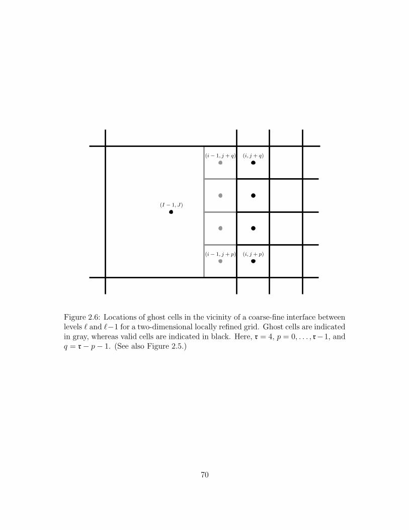
PSfrag replacements

(I − 1, J)

(i, j + p)

(i, j + q)

(i − 1, j + p)

(i − 1, j + q)

Figure 2.6: Locations of ghost cells in the vicinity of a coarse-fine interface betweenlevels ` and `−1 for a two-dimensional locally refined grid. Ghost cells are indicatedin gray, whereas valid cells are indicated in black. Here, r = 4, p = 0, . . . , r−1, andq = r− p− 1. (See also Figure 2.5.)

70

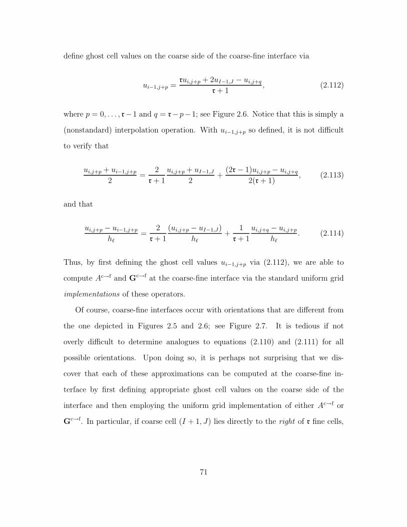
define ghost cell values on the coarse side of the coarse-fine interface via

ui−1,j+p =rui,j+p + 2uI−1,J − ui,j+q

r + 1, (2.112)

where p = 0, . . . , r−1 and q = r−p−1; see Figure 2.6. Notice that this is simply a

(nonstandard) interpolation operation. With ui−1,j+p so defined, it is not difficult

to verify that

ui,j+p + ui−1,j+p

2=

2

r + 1

ui,j+p + uI−1,J

2+

(2r− 1)ui,j+p − ui,j+q

2(r + 1), (2.113)

and that

ui,j+p − ui−1,j+p

h`=

2

r + 1

(ui,j+p − uI−1,J)

h`+

1

r + 1

ui,j+q − ui,j+p

h`. (2.114)

Thus, by first defining the ghost cell values ui−1,j+p via (2.112), we are able to

compute Ac→f and Gc→f at the coarse-fine interface via the standard uniform grid

implementations of these operators.

Of course, coarse-fine interfaces occur with orientations that are different from

the one depicted in Figures 2.5 and 2.6; see Figure 2.7. It is tedious if not

overly difficult to determine analogues to equations (2.110) and (2.111) for all

possible orientations. Upon doing so, it is perhaps not surprising that we dis-

cover that each of these approximations can be computed at the coarse-fine in-

terface by first defining appropriate ghost cell values on the coarse side of the

interface and then employing the uniform grid implementation of either Ac→f or

Gc→f. In particular, if coarse cell (I + 1, J) lies directly to the right of r fine cells,

71

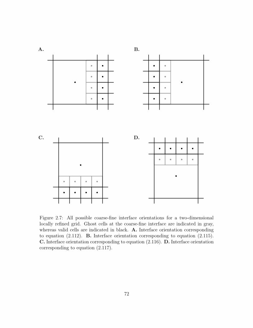
PSfrag replacements

A. B.

C. D.

Figure 2.7: All possible coarse-fine interface orientations for a two-dimensionallocally refined grid. Ghost cells at the coarse-fine interface are indicated in gray,whereas valid cells are indicated in black. A. Interface orientation correspondingto equation (2.112). B. Interface orientation corresponding to equation (2.115).C. Interface orientation corresponding to equation (2.116). D. Interface orientationcorresponding to equation (2.117).

72

(i+ r− 1, j), . . . , (i+ r− 1, j + r− 1), the coarse-fine ghost cell values are defined

by

ui+r,j+p =rui+r−1,j+p + 2uI+1,J − ui+r−1,j+q

r + 1, (2.115)

where p = 0, . . . , r− 1 and q = r− p− 1. If coarse cell (I, J + 1) lies directly above

r fine cells, (i, j + r− 1), . . . , (i+ r− 1, j + r− 1), the coarse-fine ghost cell values

are determined by

ui+p,j+r =rui+p,j+r−1 + 2uI,J+1 − ui+q,j+r−1

r + 1, (2.116)

whereas if coarse cell (I, J−1) lies directly below r fine cells, (i, j), . . . , (i+ r− 1, j),

the coarse-fine ghost cell values are determined by

ui+p,j−1 =rui+p,j + 2uI,J−1 − ui+q,j

r + 1. (2.117)

Thus, by first making use of the (virtually identical) equations (2.112)–(2.117) to

define the ghost cell values, we can simply reuse the uniform grid implementations

of Ac→f and Gc→f when computing their composite grid counterparts! In particular,

once equations (2.112)–(2.117) have been employed to determine the level ` ghost

cell values on the coarse side of the coarse-fine interface, we use the uniform grid

forms of Ac→f and Gc→f without modification throughout throughout level `. After

doing so, the values computed on the level ` cell faces must be coarsened back onto

level ` − 1. In the actual implementation of these operators, care must be taken

to ensure that the coarse grid values are not accidentally overwritten with invalid

data.

73

We next turn our attention to three spatial dimensions. In this case, the relevant

Taylor expansions of u(x) evaluated at fine cell faces xi− 12,j+pj ,k+pk

can be compactly

expressed via

ui,j+pj ,k+pk

ui,j+qj ,k+qk

uI−1,J,K

=

1 h`

20 0

1 h`

2(qj − pj)h` (qk − pk)h`

1 − rh`

2

(

r−12− pj

)

h`

(

r−12− pk

)

h`

×

ui− 12,j+pj ,k+pk

(∂xu)i− 12,j+pj ,k+pk

(∂yu)i− 12,j+pj ,k+pk

(∂zu)i− 12,j+pj ,k+pk

+O(

h2`

)

where pj, pk = 0, . . . , r− 1, qj = r − pj − 1, and qk = r − pk − 1. It is not hard to

verify that

(Ac→f1 u)i− 1

2,j+pj ,k+pk

≡ (2.118)

≡ 2

r + 1

ui,j+pj ,k+pk+ uI−1,J,K

2+

(2r− 1)ui,j+pj,k+pk− ui,j+qj,k+qk

2(r + 1)

= ui− 12,j+pj ,k+pk

+O(

h2`

)

,

74

and that

(Gc→fx u)i− 1

2,j+pj ,k+pk

≡ (2.119)

≡ 2

r + 1

(

ui,j+pj,k+pk− uI−1,J,K

)

h`+

1

(r + 1)

ui,j+qj,k+qk− ui,j+pj,k+pk

h`

= (∂xu)i− 12,j+pj ,k+pk

+O (h`) .

Note the similarity between equations (2.110) and (2.118), and between equations

(2.111) and (2.119).

As in the two-dimensional case, instead of directly making use of equations

(2.118) and (2.119) to compute Ac→f and Gc→f, we first define ghost cell values on

the coarse side of the coarse-fine interface via

ui−1,j+pj ,k+pk=

rui,j+pj,k+pk+ 2uI−1,J,K − ui,j+qj,k+qk

r + 1, (2.120)

where pj, pk = 0, . . . , r− 1, qj = r− pj − 1, and qk = r− pk − 1. With these ghost

cell values so defined, it is not hard to verify that

ui,j+pj ,k+pk+ ui−1,j+pj,k+pk

2= (2.121)

=2

r + 1

ui,j+pj ,k+pk+ uI−1,J,K

2+

(2r− 1)ui,j+pj,k+pk− ui,j+qj ,k+qk

2(r + 1),

75

and that

ui,j+pj,k+pk− ui−1,j+pj ,k+pk

h`= (2.122)

=2

r + 1

(

ui,j+pj ,k+pk− uI−1,J,K

)

h`+

1

(r + 1)

ui,j+qj,k+qk− ui,j+pj,k+pk

h`.

Analogues to (2.120) corresponding to all possible three-dimensional coarse-fine

interface orientations are obtained as easily as in the two-dimensional case. Proce-

dures for correctly evaluating these composite grid operators on each level of the

patch hierarchy are outlined in Algorithms 2.3 and 2.4.

Cell centered composite grid operators

With the composite grid versions of Af→c, Ac→f, Df→c·, and Gc→f so defined, we

are ready to define their purely cell centered counterparts. As in the uniform grid

case, the composite grid cell centered divergence of a cell centered vector field,

u = (u, v, w), is approximated at cell centers on each level of the patch hierarchy

by

(D · u)i,j,k = (Df→c · Ac→fu)i,j,k. (2.123)

Away from coarse-fine interfaces, this definition of the discrete divergence is identi-

cal to its uniform grid counterpart defined by equations (2.24) and (2.25), namely

(D · u)i,j,k =ui+1,j,k − ui−1,j,k

2h`+vi,j+1,k − vi,j−1,k

2h`+wi,j,k+1 − wi,j,k−1

2h`. (2.124)

At coarse-fine interfaces, a somewhat more complicated difference stencil is implic-

itly defined by the composition of the composite grid operators Df→c· and Ac→f.

76

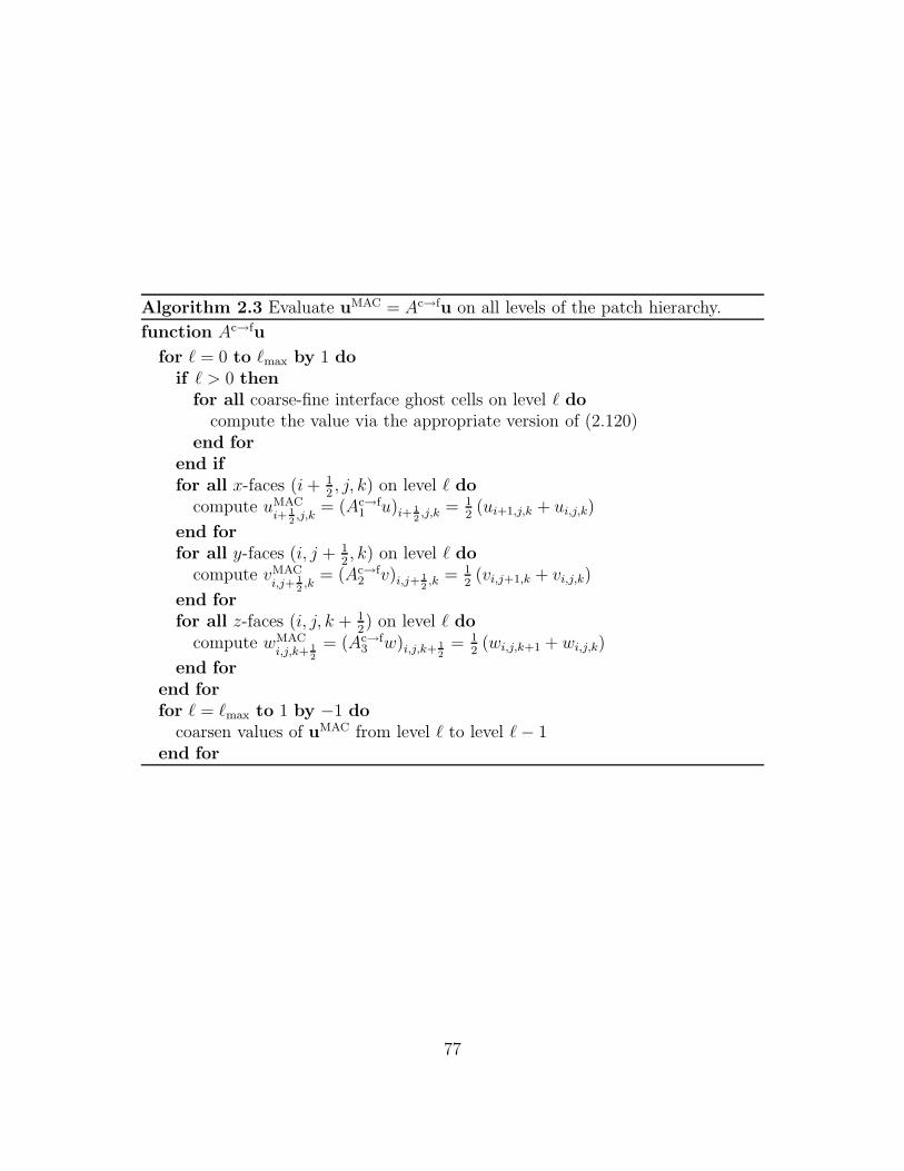
Algorithm 2.3 Evaluate uMAC = Ac→fu on all levels of the patch hierarchy.

function Ac→fu

for ` = 0 to `max by 1 do

if ` > 0 then

for all coarse-fine interface ghost cells on level ` do

compute the value via the appropriate version of (2.120)end for

end if

for all x-faces (i+ 12, j, k) on level ` do

compute uMACi+ 1

2,j,k

= (Ac→f1 u)i+ 1

2,j,k = 1

2(ui+1,j,k + ui,j,k)

end for

for all y-faces (i, j + 12, k) on level ` do

compute vMACi,j+ 1

2,k

= (Ac→f2 v)i,j+ 1

2,k = 1

2(vi,j+1,k + vi,j,k)

end for

for all z-faces (i, j, k + 12) on level ` do

compute wMACi,j,k+ 1

2

= (Ac→f3 w)i,j,k+ 1

2= 1

2(wi,j,k+1 + wi,j,k)

end for

end for

for ` = `max to 1 by −1 do

coarsen values of uMAC from level ` to level `− 1end for

77

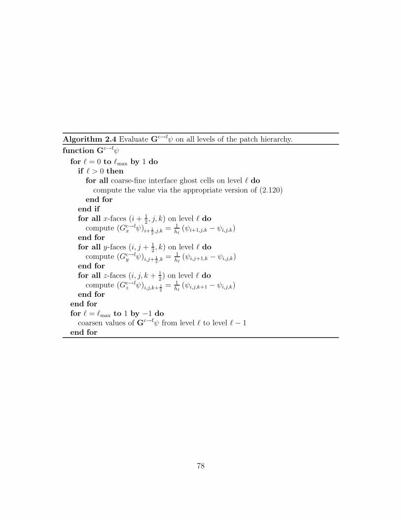
Algorithm 2.4 Evaluate Gc→fψ on all levels of the patch hierarchy.

function Gc→fψ

for ` = 0 to `max by 1 do

if ` > 0 then

for all coarse-fine interface ghost cells on level ` do

compute the value via the appropriate version of (2.120)end for

end if

for all x-faces (i+ 12, j, k) on level ` do

compute (Gc→fx ψ)i+ 1

2,j,k = 1

h`(ψi+1,j,k − ψi,j,k)

end for

for all y-faces (i, j + 12, k) on level ` do

compute (Gc→fy ψ)i,j+ 1

2,k = 1

h`(ψi,j+1,k − ψi,j,k)

end for

for all z-faces (i, j, k + 12) on level ` do

compute (Gc→fz ψ)i,j,k+ 1

2= 1

h`(ψi,j,k+1 − ψi,j,k)

end for

end for

for ` = `max to 1 by −1 do

coarsen values of Gc→fψ from level ` to level `− 1end for

78

This approximation is second order accurate away from coarse-fine interfaces but

is only first order accurate in the vicinity of a coarse-fine interface.

Likewise, the composite grid gradient of a cell centered scalar function, ψ, is

approximated at cell centers by

(Gψ)i,j,k = (Af→cGc→fψ)i,j,k. (2.125)

Again, away from coarse-fine interfaces, this composite grid definition of the discrete

gradient is identical to its uniform grid counterpart defined by equations (2.26) and

(2.27), namely

(Gψ)i,j,k =

(

ψi+1,j,k − ψi−1,j,k

2h`,ψi,j+1,k − ψi,j−1,k

2h`,ψi,j,k+1 − ψi,j,k−1

2h`

)

. (2.126)

Like the composite grid discrete divergence, the cell centered composite grid gra-

dient is second order accurate away from coarse-fine interfaces but suffers from a

localized reduction in accuracy in the vicinity of a coarse-fine interface.

Finally, the Laplacian of a cell centered scalar function, ψ, is approximated at

cell centers via

(Lψ)i,j,k = (Df→c ·Gc→fψ)i,j,k. (2.127)

Note that this discretization of the Laplace operator is symmetric [24]. Away from

the coarse-fine interface, the composite grid operator agrees with the uniform grid

79

discretization given by equation (2.29), namely

(Lψ)i,j,k =ψi+1,j,k + ψi−1,j,k − 2ψi,j,k

h2`

+ψi,j+1,k + ψi,j−1,k − 2ψi,j,k

h2`

(2.128)

+ψi,j,k+1 + ψi,j,k−1 − 2ψi,j,k

h2`

.

Like the composite grid divergence and gradient operators, the cell centered com-

posite grid approximation to the Laplacian is only second order accurate away from

coarse-fine interfaces.

Approximate and exact projections on locally refined grids

The form of the approximate cell centered projection operator for locally refined

grids is identical to its uniform grid counterpart as defined by equation (2.32) in

Section 2.3.3, namely

Pw =(

I −G (L)−1D·)

w, (2.129)

where w is a cell centered vector field defined on the locally refined Cartesian grid.

As in the uniform grid case, this operator is not a projection, since L 6= D ·G,

although for smooth u, ‖D · Pu‖ → 0 as the composite grid is refined. Similarly,

the exact MAC projection of a composite grid MAC vector field, wMAC, is given by

PMACwMAC =(

I −Gc→fL−1Df→c·)

wMAC. (2.130)

Note that, as in the uniform grid case, (Df→c · PMACwMAC)i,j,k ≡ 0.

The interested reader is referred back to Section 2.3.3 for a more complete

discussion of the relationship between the approximate cell centered projection and

80

the exact MAC projection. A major issue which we have yet to address in the

present discussion is how we go about solving systems of linear equations such as

Lϕ = D·u∗ on the composite Cartesian grid. This issue will be addressed in Chapter

3, where we describe the parallelization of the foregoing adaptive algorithm.

Local reductions in the order of accuracy

As we have frequently pointed out in the foregoing discussion, whereas the com-

posite grid interpolation operators Ac→f and Af→c retain the global second order

accuracy of their uniform grid counterparts, each of the composite grid finite differ-

ence approximations is only second order accurate away from coarse-fine interfaces

in the locally refined grid. In the vicinity of such interfaces, each of the composite

grid finite difference operators employed in the present work is only first order ac-

curate. Luckily, such localized reductions in the accuracy of the discretizations are

acceptable (if not desirable) since, at least when solving elliptic problems, it is well

known that reducing the order of accuracy on lower dimensional interfaces within

the computational domain does not alter the global accuracy of the the solution.

It has been shown analytically that a composite grid discretization of the Laplace

operator like that employed in the present work is of order h3/2 [24], and in prac-

tice we observe empirical second order convergence rates for the adaptive immersed

boundary method so long as the test problem is sufficiently smooth.

Even though they do not seem to prevent the scheme from attaining global sec-

ond order accuracy, localized reductions in accuracy could be avoided altogether by

employing higher order approximations at the coarse-fine interface. In the case of

the discrete gradient operator, this has been done in previous projection methods for

81

locally refined grids [55, 2, 42], where quadratic interpolation is employed to obtain

a more accurate approximation to the gradient at the coarse-fine interface. Im-

plementing the quadratic discretization at coarse-fine interfaces is somewhat more

involved than the present approach since additional coarse grid values are used in

the discretization. For some coarse-fine interface configurations, it is not even possi-

ble to perform the full coarse grid quadratic interpolation [42]. Since this quadratic

approximation to the gradient has generally been paired with the same composite

grid divergence operator as that used in the present work, the resulting composite

grid discretization of ∇2 still suffers from a localized reduction in accuracy near

coarse-fine interfaces. Moreover, this discretization is nonsymmetric, unlike the

discretization employed in the present work.

Since both approaches appear to yield schemes that have essentially the same

formal order of accuracy, it would be interesting to compare directly solutions

obtained by the present approach with those obtained when the composite grid

gradient is discretized by the methods described by [55, 2, 42]. In particular, it

would be beneficial to determine if the additional difficulties introduced by employ-

ing quadratic interpolation at coarse-fine interfaces (including loss of symmetry

in the discretization of ∇2 and a more complex implementation) are justified by

improvements in the quality of the computed solution. At least in the context

the immersed boundary method, however, so long as the coarse-fine boundary dis-

cretization yields a (globally) second order accurate projection method, we suspect

that the choice of coarse-fine discretization will have little impact on the overall

quality of the computed dynamics.

82

2.4.3 Timestepping

Since all levels of the locally refined grid are advanced synchronously, the timestep-

ping scheme employed in the adaptive method is largely the same as that presented

in Section 2.3.6 for the uniform grid method. The main difference between the

adaptive and non-adaptive timestepping schemes is that in the adaptive method,

the locally refined Cartesian grid is regenerated at periodic intervals according to

the refinement criteria described in Section 2.4.1. During this adaptive regridding

process, a new patch hierarchy is generated, and each Eulerian quantity that is

maintained on the locally refined Cartesian grid must be transferred from the old

patch hierarchy to the new one. Where the old and new level ` patches overlap,

such Eulerian quantities are copied directly from the old patches to the new ones.

The remaining values on the new level ` patches are determined by interpolation

from coarser levels.

The interpolation process employed during adaptive regridding may be either

conservative or non-conservative, depending on the quantity that is being interpo-

lated. For instance, the pressure, p, is not a conserved quantity, and so it suffices

to employ simple trilinear interpolation to determine new values on level ` from

values on coarser levels. In particular, for a non-conserved quantity, those values

on the new level ` patches that are not supplied by some old level ` patch are de-

termined by performing trilinear interpolation using the nearest eight coarse grid

values. On the other hand, for uniform density incompressible flows, the velocity, u,

is a conserved quantity (because of momentum conservation), and thus maintaining

discrete conservation of u during adaptive regridding prevents spurious changes in

83

the net momentum of the system. In this case, if a value on a new level ` patch is

not supplied by some old level ` patch, it is obtained in terms of a piecewise trilinear

reconstruction of u on the next coarser level (i.e., level ` − 1) via a multidimen-

sional generalization of the monotonized central-difference (MC) limited piecewise

linear reconstruction procedure. In the multidimensional MC limited interpolation

procedure, the mean value of the reconstruction of u in a level ` − 1 coarse grid

cell (I, J,K) is set to the value uI,J,K, whereas the slope of the piecewise trilinear

reconstruction in each coordinate direction is taken to be the MC limited slope in

that direction, e.g., the slope of the reconstruction of u in the x-coordinate direction

is defined by

minmod

(

unI+1,J,K − un

I−1,J,K

2h`−1, 2un

I,J,K − unI−1,J,K

h`−1, 2un

I+1,J,K − unI,J,K

h`−1

)

,

where the minmod function of three arguments is

minmod(a, b, c) =

a, if |a| ≤ min(|a|, |b|, |c|) and sign(a) = sign(b) = sign(c),

b, if |b| ≤ min(|a|, |b|, |c|) and sign(a) = sign(b) = sign(c),

c, if |c| ≤ min(|a|, |b|, |c|) and sign(a) = sign(b) = sign(c),

0, otherwise.

Thus, if a, b, and c have the same sign, the minmod function evaluates to the one

with the smallest modulus; otherwise, it evaluates to zero. By determining the

slopes in this manner, the piecewise trilinear reconstruction retains second order

accuracy where u is smooth and avoids creating spurious maxima or minima where

u is not smooth. (See, e.g., [40] for a more detailed presentation of slope limiters,

84

including the MC limiter.) When this procedure is used to determine the new

fine grid values, the discrete integral of u (and thus the momentum of the discrete

system) is not altered by the adaptive regridding process.

As a result of the foregoing conservative interpolation procedure, the cell cen-

tered velocity, un, may no longer be “sufficiently divergence free” with respect to

the cell centered divergence operator, D·, following adaptive regridding. To address

this issue, we replace un by its approximate projection after the regridding process

is complete. Before doing so, however, we first reinitialize uMAC,n by interpolating

un from cell centers to cell faces,

uMAC,n ← Ac→fun. (2.131)

Next, we replace un by its approximate projection, i.e.,

un ← Pun. (2.132)

As usual, we simultaneously replace uMAC,n by its exact MAC projection,

uMAC,n ← PMACuMAC,n, (2.133)

without having to solve any additional systems of linear equations. This completes

our discussion of the adaptive regridding process.

We now briefly detail the remaining differences between the adaptive and uni-

form grid timestepping schemes. When we compute the explicit approximation to

the nonlinear advection term in the adaptive scheme, we are able to essentially

85

reuse the Godunov procedure described in Section 2.3.7. In order for this proce-

dure to be well-defined at coarse-fine interfaces, ghost cell values are provided on

the coarse sides of such interfaces via the foregoing conservative linear interpola-

tion procedure. Also note that prior to performing the non-conservative differencing

that determines the approximation to [(u · ∇)u]n+ 12 , all face centered values must

be properly determined on the invalid regions of coarse levels as the conservative

averages of the underlying fine grid values.

Finally, as a result of the refinement criteria outlined in Section 2.4.1, the

discretization of the interaction equations is virtually unchanged in the adaptive

scheme. In particular, since each node of the curvilinear mesh is embedded in the

finest level of the patch hierarchy, equation (2.52) becomes

X(n+1)(q, r, s) = Xn(q, r, s) (2.134)

+ ∆t∑

i,j,k∈

level `max

uni,j,k δh`max

(xi,j,k −Xn(q, r, s)) h3`max.

Recall that when velocity interpolation and force spreading are performed via a

regularized delta function with a support of d meshwidths in each coordinate di-

rection, we ensure that the physical position of each node of the curvilinear mesh

is at least dd/2e + 1 grid cells away from the nearest coarse-fine interface on level

`max. Consequently, X(n+1)(q, r, s) is well-defined by equation (2.134). Moreover,

the explicit treatment of the advection terms effectively requires that ∆t be suf-

ficiently small to prevent any curvilinear mesh node from moving more than one

meshwidth in any coordinate direction during a single timestep. In particular, the

86

time increment must satisfy a CFL condition of the form

∆t ≤ C min`∈0...`max

h`/ max(i,j,k)∈

level `

(

|uni,j,k|, |vn

i,j,k|, |wni,j,k|

)

, (2.135)

where the CFL number, C, is less than one. Consequently, for each curvilinear mesh

node, X(n+1)(q, r, s) is at least dd/2e grid cells away from the nearest coarse-fine

interface on level `max, so that Xn+1(q, r, s) is well-defined by

Xn+1(q, r, s) = Xn(q, r, s) (2.136)

+∆t

2

∑

i,j,k∈

level `max

uni,j,k δh`max

(xi,j,k −Xn(q, r, s)) h3`max+

+∑

i,j,k∈

level `max

un+1i,j,k δh`max

(xi,j,k −X(n+1)(q, r, s)) h3`max

.

The remaining interaction equations, namely the analogues to equations (2.53) and

(2.54) in the uniform grid method, are treated similarly.

Note that a consequence of this explicit treatment of the Lagrangian equations

of motion is that (2.135) with C < 1 is not the only stability constraint that ∆t

must satisfy. For many applications of the immersed boundary method, it is often

necessary that ∆t = O(

h2`max

)

or even ∆t = O(

h4`max

)

to ensure the stability

of the scheme7. Thus, in practice the timestep size is frequently guaranteed to

7Although note that replacing the explicit treatment of the Lagrangian equations of motionin the present scheme with an implicit treatment would presumably free the method from theseonerous stability constraints and allow for the stable use of any C < 1 [77, 43]. Unfortunately,at the present time, the development and implementation of an implicit version of the immersedboundary method that is suitable for large scale simulation remains future work.

87

satisfy (2.135) for C 1, so that adaptively regenerating the patch hierarchy once

every nregrid = b1/Cc timesteps is sufficiently frequent to prevent the structure from

“escaping” the finest level of the hierarchy. Adaptive regridding could be performed

even less frequently by ensuring that each curvilinear mesh node is more than one

level `max grid cell away from the coarse-fine interface between levels `max − 1 and

`max. This could be accomplished, for instance, by employing larger tag buffers

when the patch hierarchy is (re-)constructed. In practice, we generally do not

make any effort to decrease the regridding frequency since regridding is typically a

small fraction of the overall computational cost of the scheme.

2.4.4 Summary of the adaptive algorithm

The adaptive algorithm is summarized as follows:

1: construct the initial patch hierarchy and initialize all state variables

2:(

u0,uMAC,0)

← project (u0)

3: set p0 = 0

4: for n = 0 to nmax by 1 do the main timestep loop

5: if mod (n, nregrid) = 0 and n > 0 then

6: regrid the patch hierarchy

7: interpolate Eulerian quantities from the old patch hierarchy to the new one

8:(

un,uMAC,n)

← project (un)

9: end if

10: for all (q, r, s) in the curvilinear mesh do see equations (2.52) and (2.134)

11: interpolate un to Xn(q, r, s) to determine Un(q, r, s)

88

12: compute X(n+1)(q, r, s) = Xn(q, r, s) + ∆tUn(q, r, s)

13: end for

14: for all (q, r, s) in the curvilinear mesh do see equations (2.53) and (2.54)

15: compute Fn(q, r, s) and F(n+1)(q, r, s) from Xn(·, ·, ·) and X(n+1)(·, ·, ·)

16: determine fn and f (n+1) by spreading Fn(q, r, s) and F(n+1)(q, r, s) to the

Cartesian grid

17: end for

18: set fn+ 12 = 1

2

(

fn + f (n+1))

19: if n = 0 then initialize the pressure

20: for m = 1 to 5 by 1 do

21: compute the explicit approximation to [(u · ∇)u]12 from u0, uMAC,0, f0,

and p0 see Section 2.3.7

22: solve equation (2.56) for u∗

23:(

u1,uMAC,1)

← project (u∗)

24: solve equations (2.66) and (2.68) to determine p12

25: p0 ← p12

26: end for

27: else use the time-lagged pressure for all timesteps n > 0

28: compute the explicit approximation to [(u · ∇)u]n+ 12 from un, uMAC,n, fn,

and pn− 12 see Section 2.3.7

29: solve equation (2.56) for u∗

30:(

un+1,uMAC,n+1)

← project (u∗)

31: solve equations (2.66) and (2.68) to determine pn+ 12

32: end if

89

33: for all (q, r, s) in the curvilinear mesh do see equations (2.69) and (2.136)

34: interpolate un+1 to X(n+1)(q, r, s) to determine U(n+1)(q, r, s)

35: compute Xn+1(q, r, s) = Xn(q, r, s) + ∆t2

(

Un(q, r, s) + U(n+1)(q, r, s))

36: end for

37: end for

In the foregoing pseudocode, note that U(·, ·, ·) is taken to be the interpolation of

the Cartesian grid velocity, u, to the nodes of the curvilinear mesh, and that the

function project (u?) is defined by Algorithm 2.5.

90

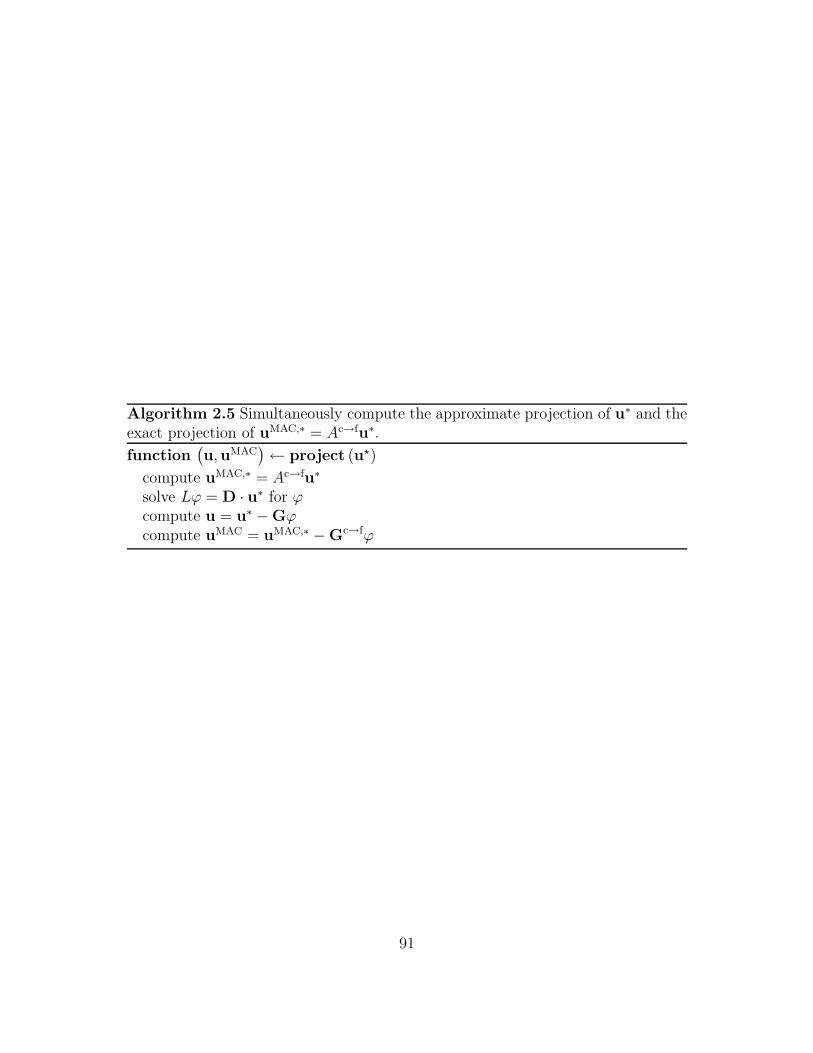
Algorithm 2.5 Simultaneously compute the approximate projection of u∗ and theexact projection of uMAC,∗ = Ac→fu∗.

function(

u,uMAC)

← project (u?)

compute uMAC,∗ = Ac→fu∗

solve Lϕ = D · u∗ for ϕcompute u = u∗ −Gϕcompute uMAC = uMAC,∗ −Gc→fϕ

91

2.5 Computational convergence results I: The lo-

cally refined projection method for the in-

compressible Navier-Stokes equations

Before examining the convergence properties of the adaptive version of the im-

mersed boundary method, we first assess the accuracy of the most complex compo-

nent of the present version of the immersed boundary method, namely the approx-

imate projection method employed for the solution of the incompressible Navier-

Stokes equations. In particular, we verify that the locally refined projection method

attains global second order convergence rates despite localized reductions in the spa-

tial order of accuracy at coarse-fine interfaces in the composite grid. Moreover, at

least for the range of grid spacings considered, we frequently observe essentially

second order pointwise convergence rates.

In [54], it is shown that the uniform grid version of the explicit Godunov pro-

cedure that is used in the present work to approximate [(u · ∇)u]n+ 12 is stable so

long as the timestep size, ∆t, satisfies

∆t ≤ h/max(i,j,k)

(|ui,j,k|, |vi,j,k|, |wi,j,k|) . (2.137)

Intuitively, for the timestep size to satisfy (2.137), ∆t must be small enough to

guarantee that any particle that is being passively advected by the flow, u, travel

less than one meshwidth in any coordinate direction during a single timestep. In the

present section, the timestep size, ∆tn, is dynamically determined at each timestep

92

n by

∆tn = C min`∈0...`max

h`/ max(i,j,k)∈

level `

(

|uni,j,k|, |vn

i,j,k|, |wni,j,k|

)

, (2.138)

where the CFL number, C, is less than one. Note that when we test the full

adaptive immersed boundary method, a more severe timestep restriction must be

imposed to ensure the stability of the scheme.

To measure convergence rates for Eulerian quantities defined on the composite

grid, we make use of various composite grid Lp norms. The discrete Lp norm of a

cell centered scalar valued function defined on the composite Cartesian grid, ψ, is

given by

‖ψi,j,k‖pp =

`max∑

`=0

∑

valid(i,j,k)∈

level `

|ψi,j,k|p h3` . (2.139)

Note that this discrete norm is only defined in terms of those values of ψ in the valid

region of each level in patch hierarchy. The L∞ norm is similarly defined, again

only in terms of the data in the valid regions of all levels in the patch hierarchy, by

‖ψi,j,k‖∞ = max`∈0...`max

maxvalid

(i,j,k)∈

level `

|ψi,j,k|. (2.140)

Analogous definitions are employed for the discrete norms of vector valued func-

tions, and appropriate modifications to these definitions are employed for two-

dimensional test cases.

In the first convergence test, we consider the solution to the two-dimensional

incompressible Navier-Stokes equations on the periodic unit square for the initial

93

conditions

u(x, 0) = 1− 2 cos(2πx) sin(2πy), (2.141)

v(x, 0) = 1 + 2 sin(2πx) cos(2πy). (2.142)

With ρ = 1, the exact solution to the incompressible Navier-Stokes equations for

these initial conditions is given by

u(x, t) = 1− 2 exp(−8π2µt) cos(2π(x− t)) sin(2π(y − t)), (2.143)

v(x, t) = 1 + 2 exp(−8π2µt) sin(2π(x− t)) cos(2π(y − t)), (2.144)

p(x, t) = − exp(−16π2µt) (cos(4π(x− t)) + cos(4π(y − t))) . (2.145)

We examine the convergence properties of the approximate projection method for

µ = 0.0001 on a composite grid with a single fixed region of localized refinement

consisting of the square defined by (x, y) ∈ (0.25, 0.75)× (0.25, 0.75) for the refine-

ment ratios r = 2 and r = 4. For comparison, we also examine the accuracy of the

method on a uniform grid. In each case, the number of grid cells in each coordinate

direction on the coarsest level, N0, is assigned the values 64, 128, 256, and 512. For

the composite grid computations, the refinement ratio, r, is held constant, so that

when the grid spacing on the coarsest level is halved, so is the grid spacing in the

refined region. The CFL number is fixed at C = 0.975, and errors and convergence

rates are assessed at t = 1. Since the same CFL number is employed in each set

of computations, note that for a fixed value of N0, the timestep size for r = 2 is

roughly twice that as for r = 4. Similarly, for a fixed value of N0, the timestep size

94

in the uniform grid case is roughly twice that as for r = 2. The results from these

sets of computations are summarized in Table 2.1.

From the data presented in Table 2.1, it is clear that over the range of grid

spacings considered, the computed values are converging to the true solution at

essentially second order rates in both the discrete L2 and L∞ norms as the uniform

and composite grids are refined. Although the second order global convergence rates

obtained in the locally refined cases are not unexpected, it is somewhat surprising

that second order pointwise convergence is observed, since the approximations to

the spatial differential operators are only first order accurate near coarse-fine in-

terfaces. Given sufficient spatial resolution, presumably the pointwise convergence

rates would drop to first order.

For µ = 0.0001 and t ∈ (0, 1),

0.9843 < exp(−16π2µt) < exp(−8π2µt) < 1, (2.146)

so that during the computed time interval, the exact solution is very nearly a trans-

lation of the initial conditions. Consequently, in the locally refined computations,

the least resolved portions of the flow (i.e., where the velocities and pressure are

least smooth) are not restricted to the locally refined region. Instead, these features

repeatedly pass through the refined region, and in particular, they repeatedly cross

the coarse-fine interface, where the spatial approximation suffers a local reduction

in accuracy. Comparing the errors obtained on a locally refined grid with an N0×N0

base grid to those obtained on a uniform N0 × N0 grid, it is clear that the locally

refined projection method generally produces solutions that are at least as accu-

95

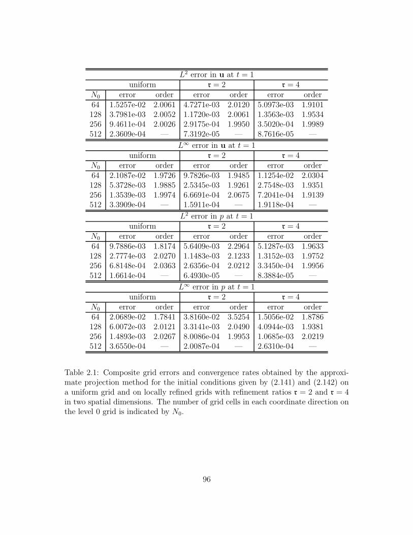
L2 error in u at t = 1uniform r = 2 r = 4

N0 error order error order error order64 1.5257e-02 2.0061 4.7271e-03 2.0120 5.0973e-03 1.9101128 3.7981e-03 2.0052 1.1720e-03 2.0061 1.3563e-03 1.9534256 9.4611e-04 2.0026 2.9175e-04 1.9950 3.5020e-04 1.9989512 2.3609e-04 — 7.3192e-05 — 8.7616e-05 —

L∞ error in u at t = 1uniform r = 2 r = 4

N0 error order error order error order64 2.1087e-02 1.9726 9.7826e-03 1.9485 1.1254e-02 2.0304128 5.3728e-03 1.9885 2.5345e-03 1.9261 2.7548e-03 1.9351256 1.3539e-03 1.9974 6.6691e-04 2.0675 7.2041e-04 1.9139512 3.3909e-04 — 1.5911e-04 — 1.9118e-04 —

L2 error in p at t = 1uniform r = 2 r = 4

N0 error order error order error order64 9.7886e-03 1.8174 5.6409e-03 2.2964 5.1287e-03 1.9633128 2.7774e-03 2.0270 1.1483e-03 2.1233 1.3152e-03 1.9752256 6.8148e-04 2.0363 2.6356e-04 2.0212 3.3450e-04 1.9956512 1.6614e-04 — 6.4930e-05 — 8.3884e-05 —

L∞ error in p at t = 1uniform r = 2 r = 4

N0 error order error order error order64 2.0689e-02 1.7841 3.8160e-02 3.5254 1.5056e-02 1.8786128 6.0072e-03 2.0121 3.3141e-03 2.0490 4.0944e-03 1.9381256 1.4893e-03 2.0267 8.0086e-04 1.9953 1.0685e-03 2.0219512 3.6550e-04 — 2.0087e-04 — 2.6310e-04 —

Table 2.1: Composite grid errors and convergence rates obtained by the approxi-mate projection method for the initial conditions given by (2.141) and (2.142) ona uniform grid and on locally refined grids with refinement ratios r = 2 and r = 4in two spatial dimensions. The number of grid cells in each coordinate direction onthe level 0 grid is indicated by N0.

96

rate as those obtained by the uniform grid method. Thus, even though the least

adequately resolved portions of the flow repeatedly cross the coarse-fine interface,

the presence of local refinement does not appear to degrade the overall quality of

the composite grid solution. Somewhat paradoxically, however, for a fixed value of

N0, the magnitude of the error for r = 4 is generally larger than that observed in

the less highly refined r = 2 case. This seeming discrepancy is explained in part

by the fact that, given the same coarse grid spacing, the truncation error at the

coarse-fine interface is slightly larger for r = 4 than it is for r = 2.

To assess the accuracy of the approximate projection method in three spatial

dimensions, we consider the solution to the incompressible Navier-Stokes equations

on the periodic unit cube for the initial conditions

u(x, 0) = 1 + cos(2πy) + sin(2πz), (2.147)

v(x, 0) = 1 + sin(2πx) + cos(2πz), (2.148)

w(x, 0) = 1 + cos(2πx) + sin(2πy). (2.149)

In the inviscid case (i.e., for µ = 0), the exact solution to the incompressible Euler

equations for these initial conditions is equal (up to a Galilean shift of the inertial

reference frame) to the Arnold-Beltrami-Childress steady solution to the three-

dimensional incompressible Euler equations (see, e.g., [23]). With ρ = 1 and µ ≥ 0,

the exact solution to the incompressible Navier-Stokes equations for these initial

97

conditions is given by

u(x, t) = 1 + exp(−4π2µt)(cos(2π(y − t)) + sin(2π(z − t))), (2.150)

v(x, t) = 1 + exp(−4π2µt)(sin(2π(x− t)) + cos(2π(z − t))), (2.151)

w(x, t) = 1 + exp(−4π2µt)(cos(2π(x− t)) + sin(2π(y − t))), (2.152)

p(x, t) =− exp(−8π2µt)× ( cos(2π(y − t)) sin(2π(z − t)) + (2.153)

sin(2π(x− t)) cos(2π(z − t)) +

cos(2π(x− t)) sin(2π(y − t)) ).

We examine the convergence properties of the approximate projection method for

µ = 0.001 on a composite grid with a single fixed region of localized refinement

consisting of the cube defined by (x, y, z) ∈ (0.25, 0.75)× (0.25, 0.75)× (0.25, 0.75)

for the refinement ratios r = 2 and r = 4. For comparison, we also examine the

accuracy of the method on a uniform grid. For the uniform grid and r = 2 cases,

the number of grid cells in each coordinate direction on the coarsest level, N0, is

assigned the values 16, 32, 64, and 128. Because of the expense of the computation,

for the r = 4 case we only consider N0 = 16, 32, and 64. For the composite grid

computations, the refinement ratio, r, is held constant, so that when the grid spacing

on the coarsest level is halved, so is the grid spacing in the refined region. The CFL

number is fixed at C = 0.975, and errors and convergence rates are assessed at

t = 1. The results from these sets of computations are summarized in Table 2.2.

As in the two-dimensional tests, from the data presented in Table 2.2, it is clear

that over the range of grid spacings considered, the computed values are converging

98

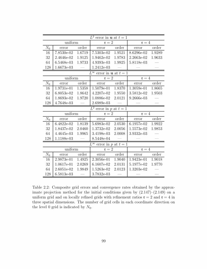
L2 error in u at t = 1uniform r = 2 r = 4

N0 error order error order error order16 7.8530e-02 1.6719 7.5303e-02 1.9521 8.6296e-02 1.928932 2.4646e-02 1.9125 1.9462e-02 1.9783 2.2663e-02 1.963364 6.5468e-03 1.9733 4.9393e-03 1.9925 5.8118e-03 —128 1.6673e-03 — 1.2412e-03 — — —

L∞ error in u at t = 1uniform r = 2 r = 4

N0 error order error order error order16 1.9731e-01 1.5358 1.5079e-01 1.8370 1.3059e-01 1.866532 6.8053e-02 1.8642 4.2207e-02 1.9550 3.5812e-02 1.950364 1.8693e-02 1.9720 1.0886e-02 2.0121 9.2666e-03 —128 4.7648e-03 — 2.6989e-03 — — —

L2 error in p at t = 1uniform r = 2 r = 4

N0 error order error order error order16 6.4822e-02 1.8139 5.6983e-02 2.0530 6.1957e-02 1.992232 1.8437e-02 2.0460 1.3732e-02 2.0056 1.5573e-02 1.985364 4.4645e-03 1.9965 3.4198e-03 2.0008 3.9332e-03 —128 1.1188e-03 — 8.5448e-04 — — —

L∞ error in p at t = 1uniform r = 2 r = 4

N0 error order error order error order16 2.9873e-01 1.4925 2.3056e-01 1.9040 1.9423e-01 1.901832 1.0617e-01 2.0269 6.1607e-02 2.0131 5.1977e-02 1.977064 2.6051e-02 1.9849 1.5263e-02 2.0123 1.3203e-02 —128 6.5813e-03 — 3.7832e-03 — — —

Table 2.2: Composite grid errors and convergence rates obtained by the approx-imate projection method for the initial conditions given by (2.147)–(2.149) on auniform grid and on locally refined grids with refinement ratios r = 2 and r = 4 inthree spatial dimensions. The number of grid cells in each coordinate direction onthe level 0 grid is indicated by N0.

99

to the true solution at essentially second order rates in both the discrete L2 and L∞

norms as the uniform and composite grids are refined. Again, although the exact

solution is roughly a translation of the initial conditions over the computed time

interval, the errors in the composite grid solutions at a fixed value of N0 compare

favorably to those in the uniform grid solution. In particular, despite the fact that

the least resolved features of the flow repeatedly cross the coarse-fine interface, the

locally refined projection method produces solutions that are at least as accurate

as those obtained by the uniform grid method. Unlike the two-dimensional results,

for a fixed value of N0, the magnitude of the pointwise error for r = 4 is generally

smaller than that observed in the less highly refined r = 2 case, although the L2

error for r = 4 is still generally larger than that of the r = 2 case.

2.6 Computational convergence results II: The

adaptive version of the immersed boundary

method

Prior to [29], the convergence of the immersed boundary method typically had been

studied computationally for problems which did not possess a sufficient degree of

smoothness for the method to attain its formal convergence rate. In particular,

most earlier convergence studies focused on the case of a viscous incompressible

fluid interacting with an infinitely thin elastic membrane (i.e., an elastic interface

or boundary). The true solutions to such problems possess discontinuities at the

interface in the pressure and in the normal derivative of the velocity, and these

100

discontinuities are not accurately captured either by the present version of the

immersed boundary method or by earlier versions of the method8.

We introduced a different approach to testing the immersed boundary method

in [29], where we considered the interaction between a viscous incompressible fluid

and a viscoelastic shell of finite thickness. This approach allowed us to assess the

performance of the uniform grid version of the present scheme in a setting where

convergence rates that corresponded to the formal order of accuracy of the method

were both anticipated and observed. (Since the shell is thin but not infinitely thin,

the discontinuities present in the true interface problem do not arise in this situa-

tion.) We follow the same approach in the present work to test the adaptive version

of the immersed boundary method. Before doing so, however, we first summarize

relevant results from [29]. Although we present in [29] empirical convergence re-

sults over a broad range of Reynolds numbers, in the present work we restrict our

attention to the moderate Reynolds number case, where Re ≈ 100.

In all of our convergence studies, the elastic properties of the shell are described

in terms of a continuum of anisotropic elastic fibers. We consider two particular

sets of elastic properties. In Section 2.6.1, we specify the stiffness of the fibers

so that the fiber tension smoothly tends to zero at the edges of the shell. As

long as the structure does not become too distorted, the resulting Cartesian elastic

force density, f , will be a continuous function of x. In Section 2.6.2, the fiber

tension is taken to be a constant multiple of |∂X/∂s|. In this case, the resulting

Cartesian elastic force density is only piecewise continuous because of the sharp

8An alternative approach is taken by the immersed interface method [41, 39], where suchdiscontinuities are explicitly accounted for by the method in a manner that yields higher orderaccuracy.

101

discontinuity in material properties that occurs at the fluid-structure interface.

For the moderate Reynolds number flows considered in the present study, where

Re ≈ 100, we observe second order or nearly second order convergence rates in

both situations. (Note that in the results presented in [29], empirical convergence

rates are observed for Re ≈ 1000 that are somewhat less than second order but

still generally in excess of first order. In those computations, it appears that under-

resolution of the velocity prevents the method from attaining full second order

convergence rates. Presumably, second order convergence would be observed even

for the high Reynolds number cases on sufficiently fine grids.)

Before proceeding to the specification of the two sets of elastic properties in

Sections 2.6.1 and 2.6.2, and the presentation of the corresponding computational

results, we first describe the common aspects for both sets of computations, in-

cluding the computational meshes used to describe the Cartesian and curvilinear

coordinate spaces, the initial conditions, and the choice of timestep.

For the two-dimensional problems considered in the present section, the physical

domain, U , is specified to be the periodic unit square and is discretized on an

adaptively refined grid. The number of grid cells in each coordinate direction on

the coarsest level (i.e., on level 0) is denoted N0, and the refinement ratio between

successive levels of resolution is r. Thus the effective grid spacing on the finest

level of the grid (i.e., on level `max) corresponds to that of a uniform grid with

N`max = r`maxN0 grid cells in each coordinate direction. Unlike the discretization of

the physical domain, the curvilinear mesh that discretizes the curvilinear coordinate

space is fixed throughout each computation. For this computational study, we take

the curvilinear coordinate space to be Ω = [0, 1]× [0, 1] (dropping the q curvilinear

102

coordinate), and we employ a fixed N r×N s computational lattice in the curvilinear

coordinate space, where N r = 38N`max and N s = 75

16N`max . With ∆r = 1/N r and

∆s = 1/N s, the “nodes” of the curvilinear mesh are the points

(r, s) = (r0, s0) + (m∆r, n∆s) =

(

∆r

2,∆s

2

)

+ (m∆r, n∆s) , (2.154)

where m ∈ 0, 1, . . . , N r − 1 and n ∈ 0, 1, . . . , N s − 1. Here, the shift by ∆r2

avoids having fibers at the exact edges of the shell, whereas the shift by ∆s2

is for

notational consistency only.

As discussed in Sections 2.2 and 2.3.4, the elastic force density generated by

the structure configuration is defined in terms of a continuum of elastic fibers, and

the curvilinear coordinates, (q, r, s), are chosen so that so that a fixed value of the

pair (q, r) labels a particular fiber for all time t, although we again emphasize that

for the present two-dimensional results we drop the q curvilinear coordinate. So

that each fiber forms a closed loop, Ω is taken to be periodic in the s-coordinate

direction. Note that s is not equal to arc length along the fibers. For this particular

Lagrangian elastic force density mapping, no boundary conditions are imposed on

the other boundaries of the curvilinear coordinate space.

The initial configuration of the viscoelastic body is given by the mapping

X(r, s, 0) =

(

1

2,1

2

)

(2.155)

+

((

α + γ

(

r − 1

2

))

cos(2πs),

(

β + γ

(

r − 1

2

))

sin(2πs)

)

,

with α = 0.2, β = 0.25, and γ = 0.0625. This expression defines the initial

103

configuration of each fiber to be an ellipse, so that the initial configuration of the

entire structure is a thick elliptical shell. The value of γ determines the thickness

of the shell and is chosen so that the thickness of the initial configuration is at

least four Cartesian meshwidths on the finest level (i.e., on level `max) of each of

the uniform or composite grids that we consider.

In all computations, the uniform density of the fluid-structure system is taken

to be ρ = 1, the uniform viscosity is taken to be µ = 0.005, and the initial velocity

of the system is taken to be u(x, 0) ≡ 0. After being released at t = 0, the shell

undergoes damped oscillations and tends toward its resting configuration, a circular

shell. The computation is halted and convergence is assessed at t = 0.4. Using the

fiber tensions specified in either Section 2.6.1 or Section 2.6.2, the shell will have

approximately completed its first oscillation at this point in the computation, and

for both sets of material properties, the corresponding flows have Re ≈ 100.

In all cases, we employ a uniform timestep that is chosen so that the computed

velocity always satisfies the composite grid CFL condition for the CFL number

C = 0.1, i.e.,

∆t < 0.1 min`∈0...`max

h`/max(i,j)∈

level `

(

|uni,j|, |vn

i,j|)

. (2.156)

This is a more severe restriction than our explicit treatment of the nonlinear ad-

vection term requires; however, since we are treating the elastic force density in

an explicit manner, the hyperbolic stability restriction is not the only stability

constraint that the timestep size must satisfy. Although (2.156) may not be suf-

ficient to ensure stability in the limit as h`max → 0, it appears to be adequate

for the uniform and composite grids considered here. To prevent the viscoelastic

104

structure from “escaping” the finest level of the hierarchical grid in the adaptive

computations, we regrid the patch hierarchy every nregrid = 8 timesteps9. For the

following computations, equation (2.156) is satisfied for ∆t = 0.08/N`max, and this

choice generally appears to result in stable computations for the grid spacings and

material parameters we consider.

Below, we present empirical convergence rates for u, p, and X in appropriately

defined discrete Lp norms for p = 1, 2. The discrete Lp norm of a cell centered

quantity defined on the locally refined Cartesian grid is defined as in Section 2.5. For

W(r, s) = (W1(r, s),W2(r, s)), a vector valued function defined on the curvilinear

mesh, the discrete Lp norm is defined by

‖W‖p =

(

∑

r,s

∣

∣W 21 (r, s) +W 2

2 (r, s)∣

∣

p/2∆r∆s

)1/p

. (2.157)

Since analytic solutions are not available for the present test cases, we compute

estimates for the convergence rates in a standard manner. In particular, for a

computed quantity, ψ, let ep[ψ;N0, L, r] denote the discrete Lp norm of the difference

in the approximation to ψ obtained on an L-level hierarchical Cartesian grid with

an N0×N0 base grid (and the corresponding uniform curvilinear mesh and uniform

timestep) and the approximation to ψ obtained on an L-level hierarchical Cartesian

grid with a 2N0 × 2N0 base grid (and the corresponding uniform curvilinear mesh

9For the present adaptive version of the immersed boundary method, adaptively regeneratingthe patch hierarchy once every nregrid = b1/Cc timesteps is sufficiently frequent to prevent thestructure from escaping the finest level of the hierarchy, where C is the maximum CFL number.

105

and uniform timestep), i.e.,

ep[ψ;N0, L, r] = ‖ψN0 − I(2N0 ,L,r)→(N0,L,r)ψ2N0‖p, (2.158)

where I(2N0 ,L,r)→(N0,L,r) denotes interpolation from finer to coarser L-level composite

grids. An empirical estimate for the convergence rate of ψ in this norm is given by

rp[ψ;N0, L, r] = log2

(

ep[ψ;N0, L, r]

ep[ψ; 2N0, L, r]

)

. (2.159)

2.6.1 Tapered elastic stiffness

For the first set of material properties, we set the fiber tension, T , via

T = σ (|∂X/∂s| ; r, s) = (1 + sin(2πr − π/2)) |∂X/∂s| . (2.160)

Recalling equations (2.11)–(2.13), the resulting Lagrangian elastic force density is

given by

F =∂

∂s(Tτ ) = (1 + sin(2πr − π/2))

∂2X

∂s2. (2.161)

In the absence of sharp corners in the elastic fibers that comprise the shell, this

Lagrangian force density smoothly tapers to zero as r approaches 0 or 1, i.e., there

is a continuous transition in material properties at the fluid-structure interface. As

long as the structure does not become too distorted, the resulting Cartesian elastic

force density, f , will remain a continuous function of x.

For our first convergence study, we use a uniform Cartesian grid discretization of

the physical domain and employ several choices for the regularized delta function,

106

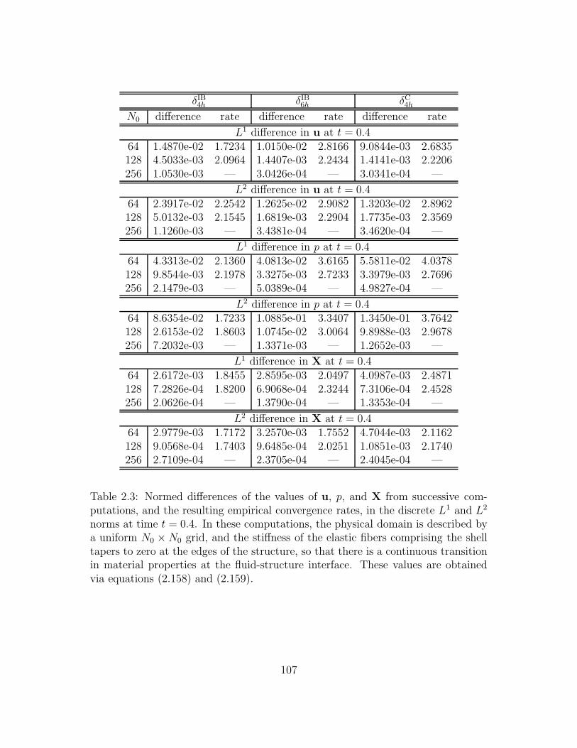
δIB4h δIB

6h δC4h

N0 difference rate difference rate difference rate

L1 difference in u at t = 0.464 1.4870e-02 1.7234 1.0150e-02 2.8166 9.0844e-03 2.6835128 4.5033e-03 2.0964 1.4407e-03 2.2434 1.4141e-03 2.2206256 1.0530e-03 — 3.0426e-04 — 3.0341e-04 —

L2 difference in u at t = 0.464 2.3917e-02 2.2542 1.2625e-02 2.9082 1.3203e-02 2.8962128 5.0132e-03 2.1545 1.6819e-03 2.2904 1.7735e-03 2.3569256 1.1260e-03 — 3.4381e-04 — 3.4620e-04 —

L1 difference in p at t = 0.464 4.3313e-02 2.1360 4.0813e-02 3.6165 5.5811e-02 4.0378128 9.8544e-03 2.1978 3.3275e-03 2.7233 3.3979e-03 2.7696256 2.1479e-03 — 5.0389e-04 — 4.9827e-04 —

L2 difference in p at t = 0.464 8.6354e-02 1.7233 1.0885e-01 3.3407 1.3450e-01 3.7642128 2.6153e-02 1.8603 1.0745e-02 3.0064 9.8988e-03 2.9678256 7.2032e-03 — 1.3371e-03 — 1.2652e-03 —

L1 difference in X at t = 0.464 2.6172e-03 1.8455 2.8595e-03 2.0497 4.0987e-03 2.4871128 7.2826e-04 1.8200 6.9068e-04 2.3244 7.3106e-04 2.4528256 2.0626e-04 — 1.3790e-04 — 1.3353e-04 —

L2 difference in X at t = 0.464 2.9779e-03 1.7172 3.2570e-03 1.7552 4.7044e-03 2.1162128 9.0568e-04 1.7403 9.6485e-04 2.0251 1.0851e-03 2.1740256 2.7109e-04 — 2.3705e-04 — 2.4045e-04 —

Table 2.3: Normed differences of the values of u, p, and X from successive com-putations, and the resulting empirical convergence rates, in the discrete L1 and L2

norms at time t = 0.4. In these computations, the physical domain is described bya uniform N0 × N0 grid, and the stiffness of the elastic fibers comprising the shelltapers to zero at the edges of the structure, so that there is a continuous transitionin material properties at the fluid-structure interface. These values are obtainedvia equations (2.158) and (2.159).

107

δh. Table 2.3 summarizes the norms of the differences in the values of u, p, and

X obtained from successive computations, and the resulting empirical convergence

rates, at time t = 0.4. These values are obtained via equations (2.158) and (2.159)

and are identical to the values reported in [29], except that in [29] the empirical

convergence rates for the Cartesian grid velocity field were reported separately for

each component of u. Second order convergence rates are observed for nearly all

computed quantities.

As shown in Table 2.3, when we employ regularized delta functions which satisfy

four moment conditions (e.g., δC4h and δIB

6h), we almost always observe convergence

rates that are in excess of second order. In particular, third order convergence rates

are observed for the pressure in several cases. One possible reason for these high

rates may be the rapid dampening of oscillations in the computed pressure as N0

increases. Recall that both δC4h and δIB

6h possess negative “tails” (see Figure 2.2).

For the coarser grid computations, these negative tails appear to induce oscillations

in the computed Eulerian quantities near the fluid-structure interface. As the spa-

tial resolution is increased, these oscillations rapidly die out, possibly resulting in

somewhat inflated estimated convergence rates.

Representative results for this particular set of material properties are displayed

in the left-hand columns of Figures 2.8–2.10, corresponding to times t = 0.08, 0.20,

and 0.32, respectively. These computed values were obtained using the six-point

delta function, δIB6h, with a uniform 512 × 512 grid, although similar results were

obtained for the other smoothed delta functions.

Next, we test the adaptive version of the immersed boundary method using

the same two-dimensional problem. For these computations, we consider only the

108

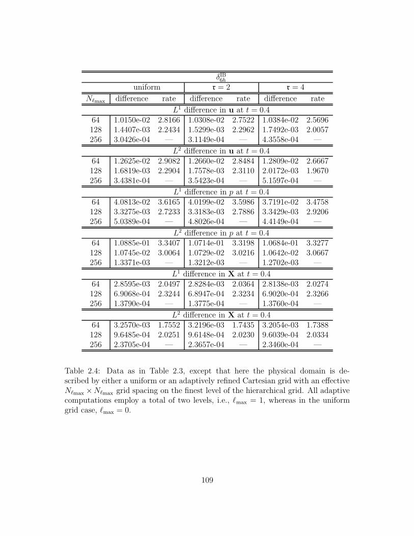
δIB6h

uniform r = 2 r = 4

N`max difference rate difference rate difference rate

L1 difference in u at t = 0.464 1.0150e-02 2.8166 1.0308e-02 2.7522 1.0384e-02 2.5696128 1.4407e-03 2.2434 1.5299e-03 2.2962 1.7492e-03 2.0057256 3.0426e-04 — 3.1149e-04 — 4.3558e-04 —

L2 difference in u at t = 0.464 1.2625e-02 2.9082 1.2660e-02 2.8484 1.2809e-02 2.6667128 1.6819e-03 2.2904 1.7578e-03 2.3110 2.0172e-03 1.9670256 3.4381e-04 — 3.5423e-04 — 5.1597e-04 —

L1 difference in p at t = 0.464 4.0813e-02 3.6165 4.0199e-02 3.5986 3.7191e-02 3.4758128 3.3275e-03 2.7233 3.3183e-03 2.7886 3.3429e-03 2.9206256 5.0389e-04 — 4.8026e-04 — 4.4149e-04 —

L2 difference in p at t = 0.464 1.0885e-01 3.3407 1.0714e-01 3.3198 1.0684e-01 3.3277128 1.0745e-02 3.0064 1.0729e-02 3.0216 1.0642e-02 3.0667256 1.3371e-03 — 1.3212e-03 — 1.2702e-03 —

L1 difference in X at t = 0.464 2.8595e-03 2.0497 2.8284e-03 2.0364 2.8138e-03 2.0274128 6.9068e-04 2.3244 6.8947e-04 2.3234 6.9020e-04 2.3266256 1.3790e-04 — 1.3775e-04 — 1.3760e-04 —

L2 difference in X at t = 0.464 3.2570e-03 1.7552 3.2196e-03 1.7435 3.2054e-03 1.7388128 9.6485e-04 2.0251 9.6148e-04 2.0230 9.6039e-04 2.0334256 2.3705e-04 — 2.3657e-04 — 2.3460e-04 —

Table 2.4: Data as in Table 2.3, except that here the physical domain is de-scribed by either a uniform or an adaptively refined Cartesian grid with an effectiveN`max ×N`max grid spacing on the finest level of the hierarchical grid. All adaptivecomputations employ a total of two levels, i.e., `max = 1, whereas in the uniformgrid case, `max = 0.

109

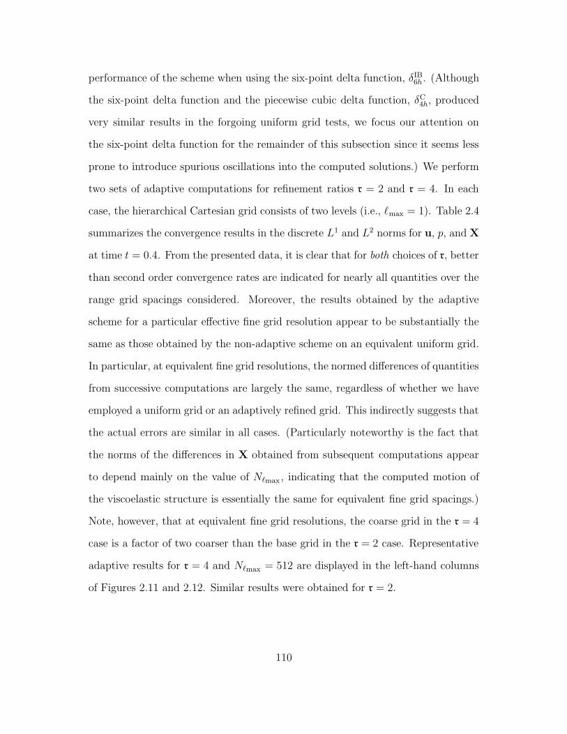
performance of the scheme when using the six-point delta function, δIB6h. (Although

the six-point delta function and the piecewise cubic delta function, δC4h, produced

very similar results in the forgoing uniform grid tests, we focus our attention on

the six-point delta function for the remainder of this subsection since it seems less

prone to introduce spurious oscillations into the computed solutions.) We perform

two sets of adaptive computations for refinement ratios r = 2 and r = 4. In each

case, the hierarchical Cartesian grid consists of two levels (i.e., `max = 1). Table 2.4

summarizes the convergence results in the discrete L1 and L2 norms for u, p, and X

at time t = 0.4. From the presented data, it is clear that for both choices of r, better

than second order convergence rates are indicated for nearly all quantities over the

range grid spacings considered. Moreover, the results obtained by the adaptive

scheme for a particular effective fine grid resolution appear to be substantially the

same as those obtained by the non-adaptive scheme on an equivalent uniform grid.

In particular, at equivalent fine grid resolutions, the normed differences of quantities

from successive computations are largely the same, regardless of whether we have

employed a uniform grid or an adaptively refined grid. This indirectly suggests that

the actual errors are similar in all cases. (Particularly noteworthy is the fact that

the norms of the differences in X obtained from subsequent computations appear

to depend mainly on the value of N`max , indicating that the computed motion of

the viscoelastic structure is essentially the same for equivalent fine grid spacings.)

Note, however, that at equivalent fine grid resolutions, the coarse grid in the r = 4

case is a factor of two coarser than the base grid in the r = 2 case. Representative

adaptive results for r = 4 and N`max = 512 are displayed in the left-hand columns

of Figures 2.11 and 2.12. Similar results were obtained for r = 2.

110

A.

B.

C.

Figure 2.8: Computed values of u, p, and f for a shell with tapered (left-handcolumn) and constant (right-hand column) elastic stiffnesses, displayed at t = 0.08.The velocity and pressure are displayed in the top row, whereas the x- and y-components of f are displayed in the middle and bottom row, respectively. Forthese computations, we use δIB

6h with ρ = 1 and µ = 0.005, and we employ auniform 512× 512 Cartesian grid.

111

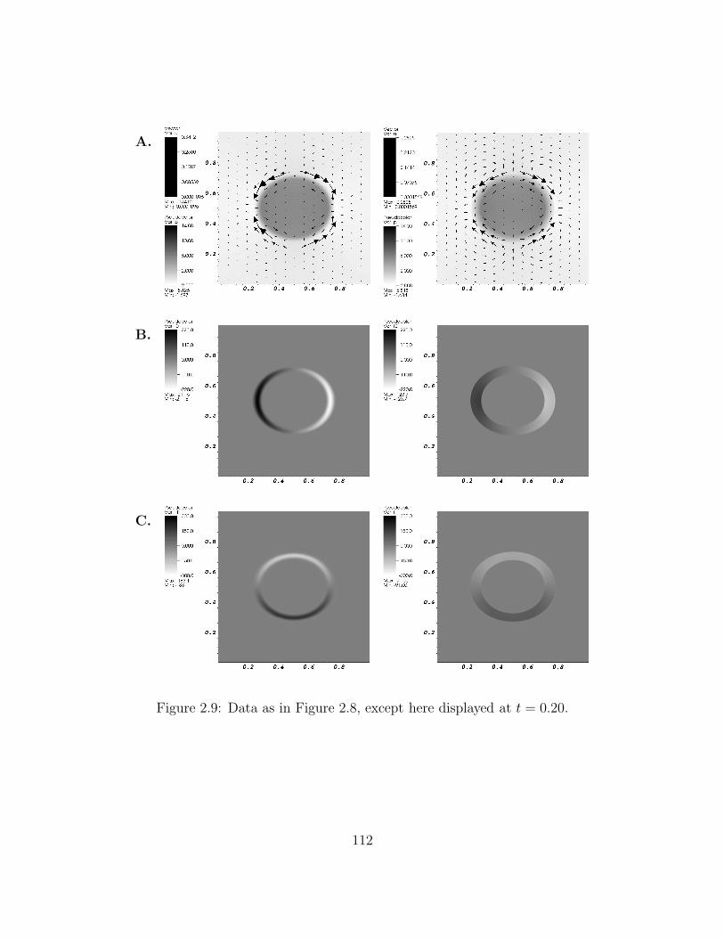
A.

B.

C.

Figure 2.9: Data as in Figure 2.8, except here displayed at t = 0.20.

112

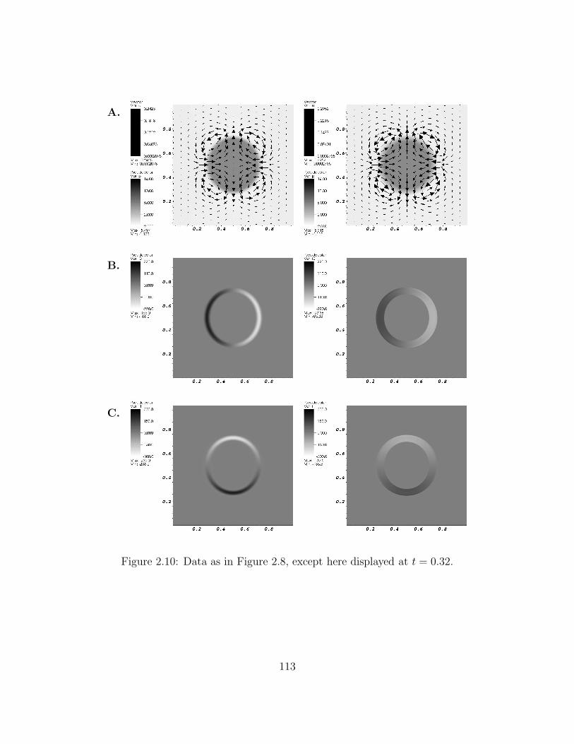
A.

B.

C.

Figure 2.10: Data as in Figure 2.8, except here displayed at t = 0.32.

113

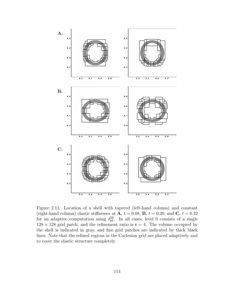
A.

B.

C.

Figure 2.11: Location of a shell with tapered (left-hand column) and constant(right-hand column) elastic stiffnesses at A. t = 0.08, B. t = 0.20, and C. t = 0.32for an adaptive computation using δIB

6h. In all cases, level 0 consists of a single128 × 128 grid patch, and the refinement ratio is r = 4. The volume occupied bythe shell is indicated in gray, and fine grid patches are indicated by thick blacklines. Note that the refined regions in the Cartesian grid are placed adaptively andto cover the elastic structure completely.

114

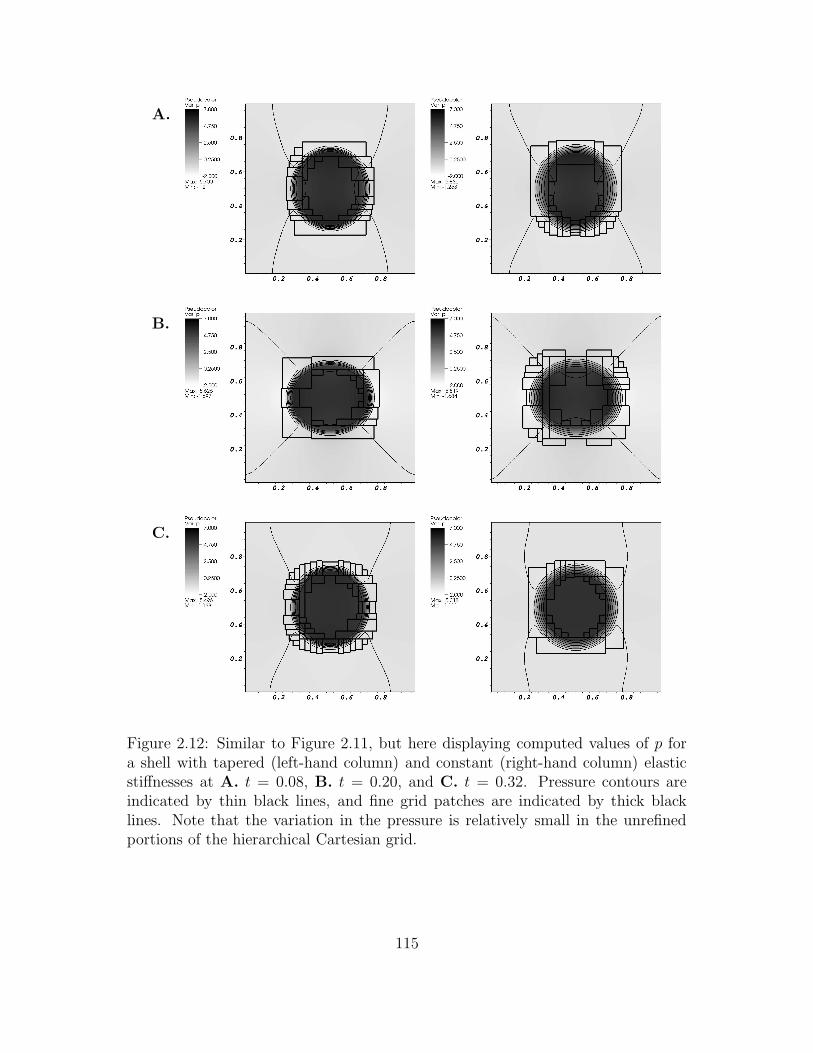
A.

B.

C.

Figure 2.12: Similar to Figure 2.11, but here displaying computed values of p fora shell with tapered (left-hand column) and constant (right-hand column) elasticstiffnesses at A. t = 0.08, B. t = 0.20, and C. t = 0.32. Pressure contours areindicated by thin black lines, and fine grid patches are indicated by thick blacklines. Note that the variation in the pressure is relatively small in the unrefinedportions of the hierarchical Cartesian grid.

115

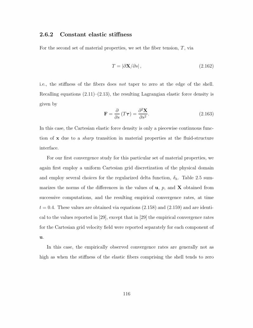
2.6.2 Constant elastic stiffness

For the second set of material properties, we set the fiber tension, T , via

T = |∂X/∂s| , (2.162)

i.e., the stiffness of the fibers does not taper to zero at the edge of the shell.

Recalling equations (2.11)–(2.13), the resulting Lagrangian elastic force density is

given by

F =∂

∂s(Tτ ) =

∂2X

∂s2. (2.163)

In this case, the Cartesian elastic force density is only a piecewise continuous func-

tion of x due to a sharp transition in material properties at the fluid-structure

interface.

For our first convergence study for this particular set of material properties, we

again first employ a uniform Cartesian grid discretization of the physical domain

and employ several choices for the regularized delta function, δh. Table 2.5 sum-

marizes the norms of the differences in the values of u, p, and X obtained from

successive computations, and the resulting empirical convergence rates, at time

t = 0.4. These values are obtained via equations (2.158) and (2.159) and are identi-

cal to the values reported in [29], except that in [29] the empirical convergence rates

for the Cartesian grid velocity field were reported separately for each component of

u.

In this case, the empirically observed convergence rates are generally not as

high as when the stiffness of the elastic fibers comprising the shell tends to zero

116

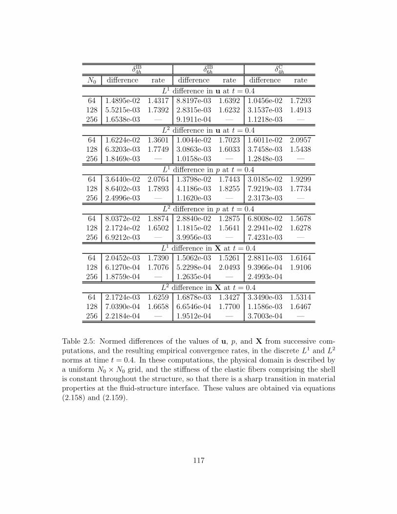
δIB4h δIB

6h δC4h

N0 difference rate difference rate difference rate

L1 difference in u at t = 0.464 1.4895e-02 1.4317 8.8197e-03 1.6392 1.0456e-02 1.7293128 5.5215e-03 1.7392 2.8315e-03 1.6232 3.1537e-03 1.4913256 1.6538e-03 — 9.1911e-04 — 1.1218e-03 —

L2 difference in u at t = 0.464 1.6224e-02 1.3601 1.0044e-02 1.7023 1.6011e-02 2.0957128 6.3203e-03 1.7749 3.0863e-03 1.6033 3.7458e-03 1.5438256 1.8469e-03 — 1.0158e-03 — 1.2848e-03 —

L1 difference in p at t = 0.464 3.6440e-02 2.0764 1.3798e-02 1.7443 3.0185e-02 1.9299128 8.6402e-03 1.7893 4.1186e-03 1.8255 7.9219e-03 1.7734256 2.4996e-03 — 1.1620e-03 — 2.3173e-03 —

L2 difference in p at t = 0.464 8.0372e-02 1.8874 2.8840e-02 1.2875 6.8008e-02 1.5678128 2.1724e-02 1.6502 1.1815e-02 1.5641 2.2941e-02 1.6278256 6.9212e-03 — 3.9956e-03 — 7.4231e-03 —

L1 difference in X at t = 0.464 2.0452e-03 1.7390 1.5062e-03 1.5261 2.8811e-03 1.6164128 6.1270e-04 1.7076 5.2298e-04 2.0493 9.3966e-04 1.9106256 1.8759e-04 — 1.2635e-04 — 2.4993e-04

L2 difference in X at t = 0.464 2.1724e-03 1.6259 1.6878e-03 1.3427 3.3490e-03 1.5314128 7.0390e-04 1.6658 6.6546e-04 1.7700 1.1586e-03 1.6467256 2.2184e-04 — 1.9512e-04 — 3.7003e-04 —

Table 2.5: Normed differences of the values of u, p, and X from successive com-putations, and the resulting empirical convergence rates, in the discrete L1 and L2

norms at time t = 0.4. In these computations, the physical domain is described bya uniform N0 × N0 grid, and the stiffness of the elastic fibers comprising the shellis constant throughout the structure, so that there is a sharp transition in materialproperties at the fluid-structure interface. These values are obtained via equations(2.158) and (2.159).

117

near the edge of the structure. This is not surprising since, unlike the tapered

case, the Cartesian force density in this case is in fact discontinuous. Nonetheless,

convergence rates at or near second order are generally indicated, although it is

possible that full second order convergence rates are not observed because of under-

resolution of the velocity in the vicinity of very narrow vorticity layers that form

near the fluid-structure interface. These vorticity layers appear well resolved for

N0 = 256 and N0 = 512, but not for N0 = 128.

Representative results for this choice of material properties are displayed in the

right-hand columns of Figures 2.8–2.10, corresponding to times t = 0.08, 0.20, and

0.32, respectively. These computed values were obtained using the six-point delta

function, δIB6h, with a uniform 512×512 grid, although similar results were obtained

for the other delta functions.

Next, we test the adaptive version of the immersed boundary method using the

same two-dimensional problem. As in the previous subsection, for these compu-

tations, we consider only the performance of the scheme when using the six-point

delta function, δIB6h. We again perform two sets of adaptive computations for refine-

ment ratios r = 2 and r = 4. In each case, the hierarchical Cartesian grid consists

of two levels (i.e., `max = 1). Table 2.6 summarizes the convergence results in the

discrete L1 and L2 norms for u, p, and X at time t = 0.4. From the presented data,

it is clear that for the range of grid spacings considered, the adaptive scheme again

achieves convergence rates that are essentially the same as those observed for the

uniform discretization, and for both choices of r, the results obtained by the adap-

tive scheme for a particular effective fine grid resolution appear to be substantially

the same as those obtained by the non-adaptive scheme on an equivalent uniform

118

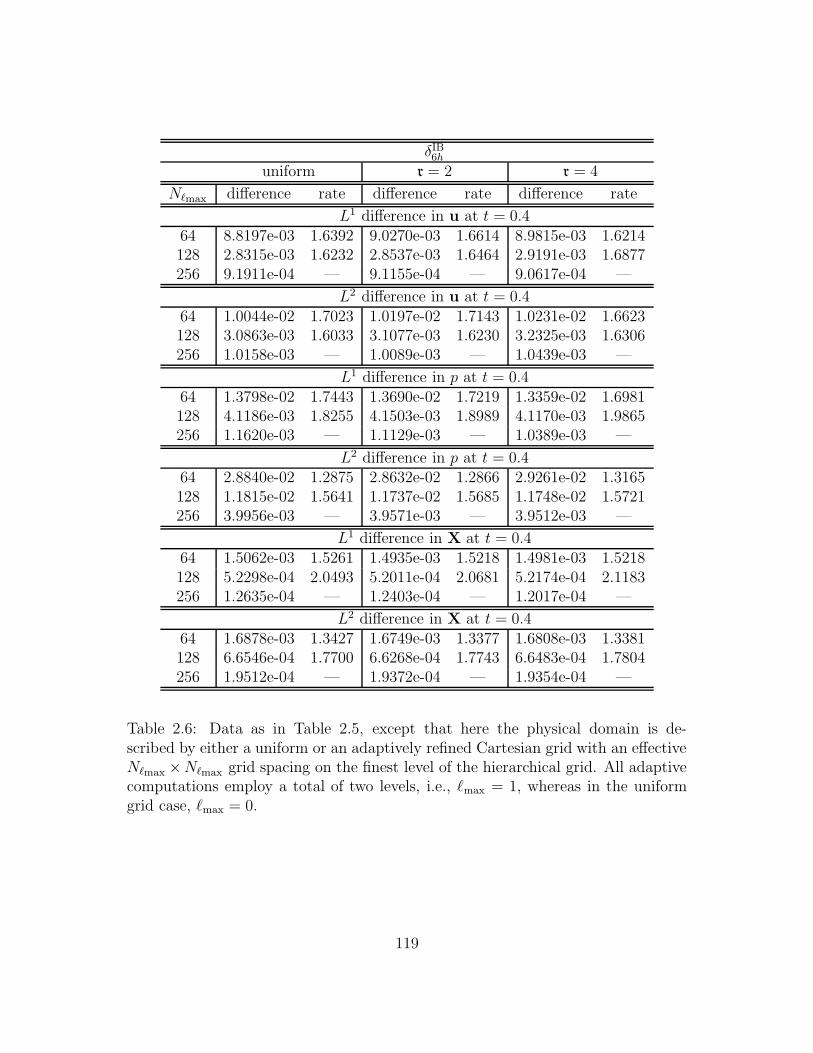
δIB6h

uniform r = 2 r = 4

N`max difference rate difference rate difference rate

L1 difference in u at t = 0.464 8.8197e-03 1.6392 9.0270e-03 1.6614 8.9815e-03 1.6214128 2.8315e-03 1.6232 2.8537e-03 1.6464 2.9191e-03 1.6877256 9.1911e-04 — 9.1155e-04 — 9.0617e-04 —

L2 difference in u at t = 0.464 1.0044e-02 1.7023 1.0197e-02 1.7143 1.0231e-02 1.6623128 3.0863e-03 1.6033 3.1077e-03 1.6230 3.2325e-03 1.6306256 1.0158e-03 — 1.0089e-03 — 1.0439e-03 —

L1 difference in p at t = 0.464 1.3798e-02 1.7443 1.3690e-02 1.7219 1.3359e-02 1.6981128 4.1186e-03 1.8255 4.1503e-03 1.8989 4.1170e-03 1.9865256 1.1620e-03 — 1.1129e-03 — 1.0389e-03 —

L2 difference in p at t = 0.464 2.8840e-02 1.2875 2.8632e-02 1.2866 2.9261e-02 1.3165128 1.1815e-02 1.5641 1.1737e-02 1.5685 1.1748e-02 1.5721256 3.9956e-03 — 3.9571e-03 — 3.9512e-03 —

L1 difference in X at t = 0.464 1.5062e-03 1.5261 1.4935e-03 1.5218 1.4981e-03 1.5218128 5.2298e-04 2.0493 5.2011e-04 2.0681 5.2174e-04 2.1183256 1.2635e-04 — 1.2403e-04 — 1.2017e-04 —

L2 difference in X at t = 0.464 1.6878e-03 1.3427 1.6749e-03 1.3377 1.6808e-03 1.3381128 6.6546e-04 1.7700 6.6268e-04 1.7743 6.6483e-04 1.7804256 1.9512e-04 — 1.9372e-04 — 1.9354e-04 —

Table 2.6: Data as in Table 2.5, except that here the physical domain is de-scribed by either a uniform or an adaptively refined Cartesian grid with an effectiveN`max ×N`max grid spacing on the finest level of the hierarchical grid. All adaptivecomputations employ a total of two levels, i.e., `max = 1, whereas in the uniformgrid case, `max = 0.

119

grid. Representative adaptive results for r = 4 and N`max = 512 are displayed in

the right-hand columns of Figures 2.11 and 2.12. Similar results were obtained for

r = 2.

2.7 Hybrid approximate projection methods

Historically, projection methods have generally used the solution to a single pro-

jection equation at each timestep to determine both the updated velocity and the

updated pressure (see [18, 19, 11], among many others). One alternative approach

is to define the updated pressure in terms of a projection that is different from that

used to obtain the updated velocity. When exact projection operators (i.e., projec-

tions that exactly enforce the discrete incompressibility of the updated velocity in

exact arithmetic) are used on periodic computational domains, there is generally no

reason to employ an additional projection, since the value of the computed velocity,

un+1, is unaffected by the approximation made to the true pressure gradient used

to obtain the intermediate velocity, u∗. This is because the approximation to the

true pressure gradient used to obtain the intermediate velocity is exactly removed

from u∗ by an exact projection. Even when physical (i.e., non-periodic) boundaries

are present, the approximation to the true pressure gradient typically influences

the velocity primarily near the physical boundary. When approximate projections

are used in place of exact ones, the situation is more complicated, since the approx-

imation to the true pressure gradient used to compute u∗ is only approximately

corrected by the projection.

For uniform grid discretizations, it is well known that even exact cell centered

120

projection methods can introduce nonphysical oscillations because the operator

D ·G possesses a nontrivial nullspace (resulting in so-called checkerboard modes).

Approximate cell centered projection methods can exacerbate this problem by pro-

ducing computed velocities that are contaminated by components that are non-

solenoidal with respect to the cell centered divergence operator, a problem that

is further compounded in the presence of local grid refinement. A common ap-

proach to dealing with these difficulties is to stably filter the undesirable compo-

nents (i.e., the components corresponding to the nonsolenoidal and checkerboard

modes) from the computed velocity [36, 65, 21]. An alternative approach to im-

proving the quality of the computed solution was suggested by Almgren et al. [3],

who introduced a hybrid approximate projection method for the incompressible

Euler equations. (The uniform grid approximate projection method presented in

Section 2.3.6 is one possible extension of this method to the viscous case.) In the

hybrid approximate projection approach of Almgren et al., two different interme-

diate velocities are determined at each timestep from two different treatments of

the momentum equation. Each intermediate velocity is approximately projected,

with the first projection determining the updated velocity and the second yielding

the updated pressure. This approach is clearly more computationally demanding

than simply determining the velocity and pressure in terms of a single approxi-

mate projection10. To justify this additional computational cost and algorithmic

complexity, we demonstrate below that nonphysical oscillations can occur in the

10The computational cost of the hybrid projection method can be reduced by solving for thedifference in the solutions to the two projection equations rather than solving a second projectionequation. Since an accurate initial guess for this difference is available, the resulting equationfrequently needs to be solved only to a loose relative error tolerance.

121

computed pressure when a more “traditional” projection method is used (i.e., a

projection method that obtains the updated velocity and pressure in terms of a

single treatment of the momentum equation and the solution to a single projection

at each timestep). These oscillations, sometimes considered to be a characteristic

of the immersed boundary method [39], are virtually eliminated by making use of

our hybrid method. In the adaptively refined case, we also demonstrate that the

use of the hybrid method suppresses long-range pressure oscillations which occur

when the traditional projection method is employed.

2.7.1 A more traditional approximate projection method

Before demonstrating the reduction in nonphysical oscillations provided by our hy-

brid method, we must briefly describe the more traditional second order projection

method that we compare to the hybrid scheme. This method is essentially a version

of the projection method of Bell, Colella, and Glaz (BCG) [11], making use of a

modification similar to one introduced by Brown et al. [16] to obtain full second

order accuracy in the pressure. We refer to the resulting scheme as a “BCG-like”

approximate projection method. For this method, the velocity, denoted u, and

pressure, denoted p, are both obtained in terms of the solution to the same pro-

jection equation. It is important to emphasize that since we are making use of

approximate projections, it is generally the case that u 6= u and p 6= p, where u

and p are the velocity and pressure obtained via the hybrid approximate projection

method of Section 2.3.6.

122

In the BCG-like method, the intermediate velocity is determined by

(I − η2νL)(I − η1νL)u∗ = (2.164)

= (I + η3νL)un + ∆t(I + η4νL)

(

−Nn+ 12 +

1

ρ

(

fn+ 12 −Gpn− 1

2

)

)

.

Next, un+1 is given by approximately projecting u∗, i.e.,

u∗ = un+1 + Gϕ, (2.165)

where

Lϕ = D · u∗. (2.166)

The pressure consistent with this treatment of the incompressible Navier-Stokes

equations can be obtained in a manner similar to that previously used to determine

the updated pressure in the hybrid scheme. In this case, the updated pressure is

the scalar function pn+ 12 given by

pn+ 12 = pn− 1

2 +ρ

∆t(I + η4νL)−1(I − η2νL)(I − η1νL)ϕ. (2.167)

2.7.2 Reducing nonphysical pressure oscillations

To demonstrate the effectiveness of our hybrid approximate projection method in

reducing nonphysical oscillations when compared to a BCG-like projection method,

we consider a two-dimensional fluid-structure interaction problem similar to those

described in Section 2.6, but here we restrict the curvilinear coordinate space to

123

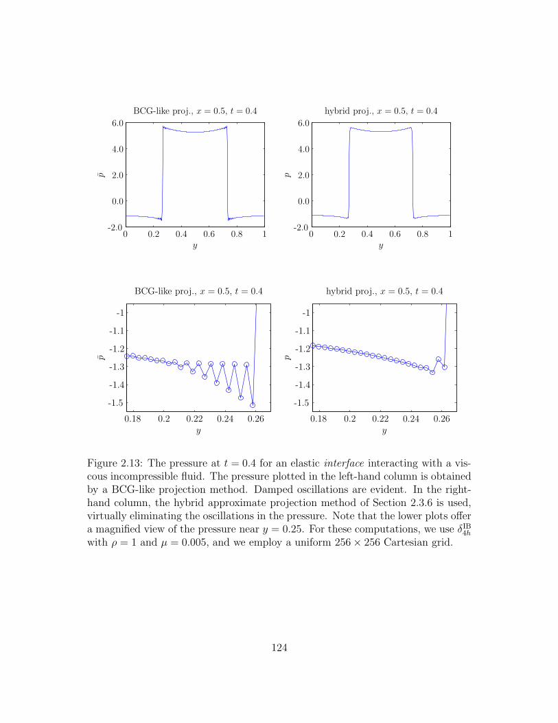
PSfrag replacements

y

pBCG-like proj., x = 0.5, t = 0.4

0 0.2 0.4 0.6 0.8 1-2.0

0.0

2.0

4.0

6.0

PSfrag replacements

y

p

hybrid proj., x = 0.5, t = 0.4

0 0.2 0.4 0.6 0.8 1-2.0

0.0

2.0

4.0

6.0

PSfrag replacements

y

p

BCG-like proj., x = 0.5, t = 0.4

0.18 0.2 0.22 0.24 0.26

-1.5

-1.4

-1.3

-1.2

-1.1

-1

PSfrag replacements

y

phybrid proj., x = 0.5, t = 0.4

0.18 0.2 0.22 0.24 0.26

-1.5

-1.4

-1.3

-1.2

-1.1

-1

Figure 2.13: The pressure at t = 0.4 for an elastic interface interacting with a vis-cous incompressible fluid. The pressure plotted in the left-hand column is obtainedby a BCG-like projection method. Damped oscillations are evident. In the right-hand column, the hybrid approximate projection method of Section 2.3.6 is used,virtually eliminating the oscillations in the pressure. Note that the lower plots offera magnified view of the pressure near y = 0.25. For these computations, we use δIB

4h

with ρ = 1 and µ = 0.005, and we employ a uniform 256× 256 Cartesian grid.

124

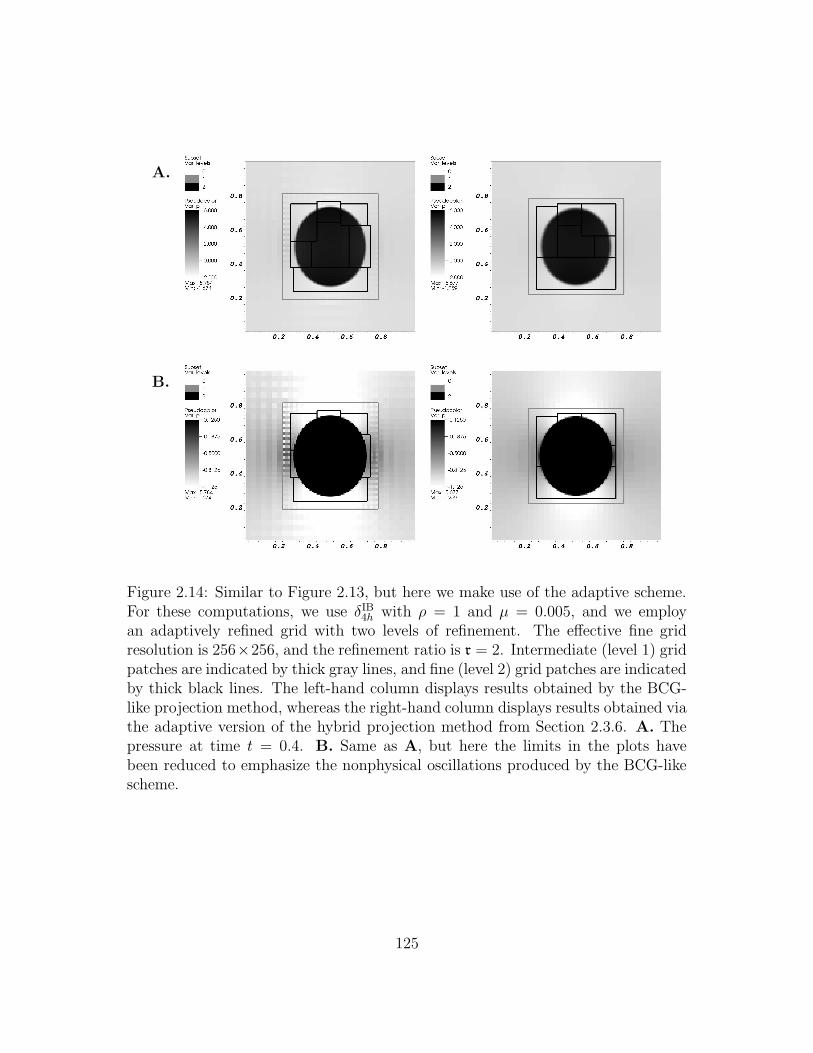
A.

B.

Figure 2.14: Similar to Figure 2.13, but here we make use of the adaptive scheme.For these computations, we use δIB

4h with ρ = 1 and µ = 0.005, and we employan adaptively refined grid with two levels of refinement. The effective fine gridresolution is 256×256, and the refinement ratio is r = 2. Intermediate (level 1) gridpatches are indicated by thick gray lines, and fine (level 2) grid patches are indicatedby thick black lines. The left-hand column displays results obtained by the BCG-like projection method, whereas the right-hand column displays results obtained viathe adaptive version of the hybrid projection method from Section 2.3.6. A. Thepressure at time t = 0.4. B. Same as A, but here the limits in the plots havebeen reduced to emphasize the nonphysical oscillations produced by the BCG-likescheme.

125

Ω = [12, 1

2]× [0, 1], so that the structure is a true elastic interface. This is a situation

where the immersed boundary method can produce nonphysical oscillations in the

computed pressure near the interface [39]. Like the computations of Section 2.6, the

initial configuration is given by (2.155), although here restricted to r ≡ 12

so that

the initial configuration is an elliptical membrane. Following its release at t = 0,

the membrane undergoes damped oscillations until eventually settling in a circular

configuration. We compute the motion of the coupled system up to t = 0.4, at

which time the elastic structure has completed one full oscillation and is beginning

its second. The material properties are as described in Section 2.6.2, with ρ = 1

and µ = 0.005, and the smoothed delta function employed for these comparisons is

δIB4h.

The computation is first performed using the BCG-like approximate projection

method on a uniform 256× 256 Cartesian grid (and the corresponding curvilinear

mesh). When this traditional projection method is employed, oscillations are read-

ily observed in the computed pressure plotted in Figure 2.13, and it is clear that

these oscillations continue for many grid cells away from the interface before dying

out. When we repeat the computation, this time using the hybrid approximate

projection method of Section 2.3.6, the oscillations are virtually eliminated from

the computed pressure. As shown in Figure 2.14, similar results are obtained in the

adaptive context, but in this case the BCG-like scheme induces long-range pressure

oscillations. It appears that these long-range oscillations may be a result of partic-

ular spatial discretization at the coarse-fine interface employed in the present work,

and it may be possible to eliminate them by employing a different discretization

at such interfaces. However, by employing our hybrid projection method, we are

126

able to simultaneously eliminate both the near-boundary oscillations (such as those

displayed in Figure 2.13) and the long-range oscillations (such as those displayed in

Figure 2.14) that are exhibited by the BCG-like scheme in the immersed boundary

context.

2.8 Concluding remarks on the adaptive version

of the immersed boundary method

In the present chapter, we have introduced a formally second order accurate adap-

tive version of the immersed boundary method and examined the performance of

this scheme for a prototypical fluid-structure interaction problem. This new algo-

rithm is an extension of the uniform grid method described in [29], and both the

present adaptive method and its uniform grid counterpart are differentiated from

most previous versions of the immersed boundary method by their inclusion of sev-

eral numerical methods intended to reduce the occurrence of nonphysical oscilla-

tions in the computed dynamics. In particular, we use a strong stability-preserving

Runge-Kutta method for the time integration of the structure configuration, an im-

plicit L-stable discretization of the viscous terms in the momentum equation, and

a second order Godunov method for the explicit treatment of the nonlinear terms

in the momentum equation. We also employ a new hybrid approximate projection

method for the incompressible Navier-Stokes equations. When compared to more

traditional projection methods, we have demonstrated that this hybrid approach

dramatically reduces the occurrence of oscillations in the computed pressure for

127

both uniform and adaptively refined computations.

By considering fluid-structure interaction problems which possess sufficiently

smooth solutions, actual second order convergence rates were demonstrated in our

numerical tests of the method for moderate Reynolds number flows. Unlike most

previous convergence studies for the immersed boundary method, however, we did

not consider the interaction of a true interface and an incompressible fluid. When

the immersed boundary method is applied to such problems, second order con-

vergence rates are not observed because of the inability of the method to prop-

erly capture discontinuities in the pressure and normal derivative of the velocity

across the interface. We avoided these discontinuities by considering the interaction

of a viscoelastic shell of finite thickness and an incompressible fluid11. Although

such problems are in some sense not as difficult as true interface problems, they

are relevant to many application areas where the immersed boundary method is

used. A particular example appears in Chapter 4, where we apply the methodol-

ogy described in the present chapter to Peskin and McQueen’s model of the heart

and nearby great vessels [62, 49, 59, 63, 64, 51, 52, 53]. Although elastic surfaces

are used in this model to describe the heart valve leaflets, the description of the

muscular heart wall is analogous to a viscoelastic shell—albeit one with complex,

time-dependent elastic properties.

Finally, in the present chapter, the adaptive scheme was demonstrated to pro-

duce results that are substantially the same as those obtained by the equivalent

uniform grid method (i.e., results that are largely identical to those obtained on

11Note, however, that second order or nearly second order convergence rates were observed bothfor the case that there is a smooth transition in material properties at the fluid-structure interfaceand for the case that there is a sharp transition in material properties.

128

a uniform grid with resolution that is equal to the highest resolution employed in

the adaptive computation). In particular, the adaptive scheme was demonstrated

to yield second order or nearly second order convergence rates that were similar

to those produced by the equivalent uniform grid method. Moreover, we found

that the adaptive method produced virtually identical computed dynamics when

compared to the equivalent non-adaptive scheme. This is not a surprise, perhaps,

since in the test problems considered, the dominant errors in the computed solu-

tions appear to be localized near the fluid-structure interface. In such situations,

the least resolved portions of the solution will be embedded in the finest level of

the adaptively refined grid and will generally lie away from coarse-fine interfaces.

Nonetheless, this result has important practical implications, since it indicates that

for problems with localized fine scale features, it may be possible to obtain well

resolved simulation results by adaptively deploying very high spatial resolution in

only a limited portion of the computational domain. In order for such an adaptive

approach to translate into real-world performance gains, however, it is not enough

to simply possess an effective adaptive discretization; the adaptive scheme must be

efficiently implemented, and we shall address this important topic in the following

chapter.

129

Chapter 3

A parallel implementation of the

immersed boundary method for

distributed-memory

multiprocessor systems

3.1 Basic approaches to distributed-memory par-

allelization

Despite decades of sustained increases in computing power, obtaining well-resolved

simulation results in three spatial dimensions still generally requires the use of sig-

nificant computing resources. Correspondingly, we have implemented the adaptive

version of the immersed boundary method introduced in Chapter 2 for use on the

130

class of large scale computing platforms that is most widely available at the present

time, namely distributed-memory parallel computers. This chapter provides a high-

level overview of this parallel implementation, paying particular attention to the al-

gorithms and data structures that yield an implementation of the numerical scheme

that is sufficiently efficient to be useful for large scale simulation. Although we do

not present detailed timing results for this parallel code, the efficacy of the software

is demonstrated in part by the simulation results presented in Chapter 4. Through-

out our discussion, we highlight our use of readily available mathematical software

libraries. Indeed, we feel that the appropriate use of such libraries has played an

essential role in making the development of the present parallel implementation

and its application to simulating cardiac mechanics manageable tasks.

Modern distributed-memory parallel computers typically consist of hundreds,

thousands, or even tens of thousands of processing nodes that are connected by a

high-speed network. The defining characteristics of such machines are that each of

the nodes in the system has its own local memory, and that a particular node is

unable to access directly data that is stored in the memory of another node. In

particular, such machines do not possess a global memory address space. Instead,

when data on one node is required by another node in the system, an explicit

communication step is required to transfer the data between the two processors.

On most present distributed-memory machines, interprocess data transactions are

facilitated by a so-called message-passing library. Although these libraries generally

must be tuned to the design of a particular system and therefore are in some

sense platform-dependent, most provide at least a broad subset of the functionality

specified by the Message-Passing Interface (MPI) standard [56, 30]. Consequently,

131

distributed-memory parallel software can at least in principle be made portable,

so that it can be compiled and executed on any parallel platform that provides an

MPI-compliant communication library.

Individual nodes of a distributed-memory parallel machine may themselves be

full-fledged parallel computers. On such platforms, a given node typically consists

of a small number of processors, each of which has access to a shared local pool of

memory. Although such machines are commonly encountered, at the present time

we have only implemented support for distributed parallelism via message-passing.

Future improvements to the current implementation may be facilitated by switching

to a hybrid programming model that exploits both modes of parallelism. Such

an approach could take advantage of the substantial experience accrued from the

development and application by Peskin and McQueen of a shared-memory parallel

implementation of an earlier version of the immersed boundary method [51].

Developing a distributed-memory parallel implementation of any particular ver-

sion of the immersed boundary method requires a number of design decisions. Per-

haps the most important of these addresses the manner in which the Lagrangian

and Eulerian data is partitioned across the available processors. Among the possible

choices are:

1. Independently subdivide and distribute the Cartesian grid and the curvilinear

mesh; or

2. First subdivide and distribute the Cartesian grid (possibly doing so according

to criteria that accounts for the configuration of the curvilinear mesh); then

subdivide and distribute the curvilinear mesh so that each curvilinear mesh

132

node is assigned to the processor that “owns” the portion of the Cartesian

grid in which that node is “embedded.”

In considering these two possibilities, a third alternative may come to mind: first

partition the curvilinear mesh and then partition the Cartesian grid accordingly;

however, it is difficult to conceive of a reasonable way to implement such an ap-

proach without placing restrictions on the configuration of the curvilinear mesh.

A distributed-memory parallel implementation of an earlier version of the im-

mersed boundary method has been developed as part of the Titanium project at

the University of California at Berkeley that essentially follows the first of the afore-

mentioned approaches to partitioning the Lagrangian and Eulerian data [74]. Since

the curvilinear mesh and Cartesian grid are independently distributed amongst the

available processors, it is relatively straightforward to subdivide both in a man-

ner that results in a nearly-uniform distribution of the computational workload

associated with “purely Lagrangian” and “purely Eulerian” computations1. One

drawback to this approach is that it potentially requires a large amount of interpro-

cess communication to evaluate the discrete interaction equations. In particular,

when the four-point delta function is employed in three spatial dimensions, each

curvilinear mesh node is coupled to 64 Cartesian grid cells, and note that a partic-

ular curvilinear mesh node will not necessarily be assigned to the same processor

as that which has been assigned the data corresponding to the nearby Cartesian

grid cells. Moreover, the degree of coupling rapidly increases as the support of

1By “purely Lagrangian,” we mean computations involving only data defined on the curvilinearmesh, e.g., determining the discrete curvilinear force density, F(·, ·, ·), from the configuration ofthe elastic structure, X(·, ·, ·). Similarly, “purely Eulerian” computations involve only data thatis defined on the Cartesian grid, e.g., determining the value of the updated velocity, u

n+1, fromthe approximate projection of an intermediate velocity field.

133

the regularized delta function is broadened, and it is clear from the convergence

results presented in Chapter 2 that such delta functions can yield substantial im-

provements in the quality of the computed solutions. Nonetheless, promising initial

results have been obtained by following this approach to parallelizing the immersed

boundary method.

Our parallel implementation of the adaptive version immersed boundary method

takes the second of the above listed approaches to distributing the Eulerian and La-

grangian data and does so in a manner that we now make more precise. Before pro-

ceeding, recall that the levels of the composite grid are numbered by ` = 0, . . . , `max,

where ` = 0 indicates the coarsest level and ` = `max indicates the finest; that the

uniform grid spacing on each level of the hierarchical grid is given by h`; and that

the curvilinear mesh is embedded within the finest level of the composite Cartesian

grid. (For more details, see Section 2.4.1.) It is also convenient to define c`(i, j, k)

by

c`(i, j, k) = [ih`, (i+ 1)h`)× [jh`, (j + 1)h`)× [kh`, (k + 1)h`), (3.1)

so that c`(i, j, k) indicates the physical region that is occupied by Cartesian grid cell

(i, j, k) on level `. Each time that the composite Cartesian grid is (re-)initialized, we

require that the grid patches generated on each level of the patch hierarchy be non-

overlapping. These patches are then distributed amongst the available processors

according to load balancing criteria that attempts to account for the present config-

uration of the curvilinear mesh (see below). Once this has been accomplished, each

of the available processors has been assigned some subset of the rectangular grid

patches that comprise the hierarchical grid. Since the patches that make up each

134

level are non-overlapping, note that each Cartesian grid cell (i, j, k) on a particular

level of the hierarchy is associated with only one of the processors.

We next subdivide and distribute the curvilinear mesh. Each curvilinear mesh

node (q, r, s) is assigned to whichever processor has been assigned the particular

Cartesian grid cell (i, j, k) on level `max that satisfies X(q, r, s) ∈ c`max(i, j, k). In

other words, each curvilinear mesh node is assigned to the processor that owns the

Cartesian grid cell on level `max in which that curvilinear mesh node is embedded.

Since the grid patches on each level are required to be non-overlapping, this defines a

unique decomposition and distribution of the curvilinear mesh. Note that although

the parallel distribution of the curvilinear mesh is completely determined by the

parallel distribution of the Cartesian grid, the manner in which the Cartesian grid

patches are distributed to the processors is determined at least in part by the

configuration of the curvilinear mesh in accordance with the load balancing criteria

described below.

Defining the distribution of the Lagrangian data in terms of the distribution

of the Eulerian data in the foregoing manner ensures that relatively little inter-

process communication is required to evaluate the discrete interaction equations.

Unfortunately, this particular data distribution makes balancing the computational

workload somewhat more challenging. A reasonable approach to balancing the

purely Eulerian computational workload is to assign to each processor a subset of

the grid patches that comprise each level of the hierarchy, doing so in a manner

that attempts to ensure that the total volume of the set of patches assigned to

each processor is roughly equal. This is done on a level-by-level basis for each level

` < `max, since in the present adaptive scheme, the only computations performed

135

on those levels are purely Eulerian.

Since the parallel distribution of the Cartesian grid patches completely deter-

mines that of the curvilinear mesh, a different load balancing strategy is employed

on level `max of the composite Cartesian grid (i.e., the level in which the curvilinear

mesh is embedded). First, a workload estimate is computed in each cell on level

`max via

worki,j,k = α + β |(q, r, s) : X(q, r, s) ∈ c`max(i, j, k)| , (3.2)

i.e., the workload estimate in cell (i, j, k) is taken to be α plus β times the number of

curvilinear mesh nodes embedded in cell (i, j, k), so that α determines the relative

importance of the Eulerian workload and β determines the relative importance of

the Lagrangian workload. (Presently, we simply set α = β = 1, although these

values have not been tuned in any way. The optimal values are almost certainly

application dependent and are likely different from those that we are presently

using.) With the workload estimate so defined, the patches that comprise the

finest level of the hierarchy are distributed to the available processors in a manner

that attempts to ensure that the total estimated workload is roughly equal on each

processor. Note that a consequence of this load balancing strategy is that the

parallel distributions of both the Cartesian grid and the curvilinear mesh are able

to adapt to the configuration of the elastic structure as it evolves during the course

of a simulation.

136

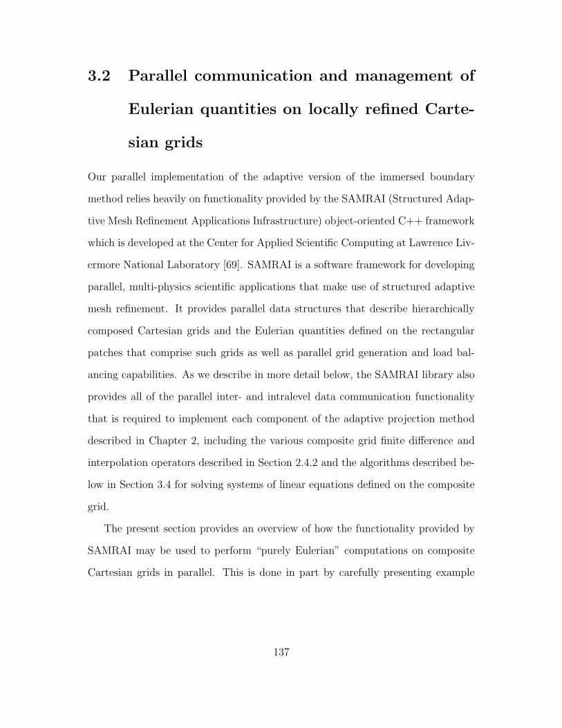
3.2 Parallel communication and management of

Eulerian quantities on locally refined Carte-

sian grids

Our parallel implementation of the adaptive version of the immersed boundary

method relies heavily on functionality provided by the SAMRAI (Structured Adap-

tive Mesh Refinement Applications Infrastructure) object-oriented C++ framework

which is developed at the Center for Applied Scientific Computing at Lawrence Liv-

ermore National Laboratory [69]. SAMRAI is a software framework for developing

parallel, multi-physics scientific applications that make use of structured adaptive

mesh refinement. It provides parallel data structures that describe hierarchically

composed Cartesian grids and the Eulerian quantities defined on the rectangular

patches that comprise such grids as well as parallel grid generation and load bal-

ancing capabilities. As we describe in more detail below, the SAMRAI library also

provides all of the parallel inter- and intralevel data communication functionality

that is required to implement each component of the adaptive projection method

described in Chapter 2, including the various composite grid finite difference and

interpolation operators described in Section 2.4.2 and the algorithms described be-

low in Section 3.4 for solving systems of linear equations defined on the composite

grid.

The present section provides an overview of how the functionality provided by

SAMRAI may be used to perform “purely Eulerian” computations on composite

Cartesian grids in parallel. This is done in part by carefully presenting example

137

code that performs a simple computation, namely the evaluation of the uniform

grid version of the Laplacian on a single level of a locally refined Cartesian grid.

Although the operation that we describe is extremely simple, the functionality

required by its implementation is much the same as that needed to implement

the more complex operations required by the adaptive version of the immersed

boundary method. Moreover, as we describe in Section 3.3, this same functionality

may be exploited to simplify the management of the distributed curvilinear mesh

and the evaluation of the Lagrangian-Eulerian interaction equations.

Of course, a complete description of the SAMRAI framework is beyond the scope

of the present work. The interested reader is referred to [69, 79, 33, 80] for more

detailed discussions of the design, implementation, and application of SAMRAI.

3.2.1 Variables, patch data factories, and patch data

SAMRAI conceptually separates variables from their associated data storage. In the

implementation of non-adaptive numerical methods, there is little reason to make

such a distinction, since the data associated with a particular variable (e.g., in the

present context, the cell centered Eulerian velocity field, u) typically has a static

representation (e.g., a fixed-size array in memory of double precision values). This

is not the case in an adaptive computation, since the grid on which the problem is

discretized is frequently modified to account for the evolving state of the computed

solution. Consequently, the form of the data storage associated with a particular

variable is necessarily non-static.

In SAMRAI, variable objects specify properties that are independent of the

138

particular configuration of the patch hierarchy; consequently, these objects typi-

cally persist throughout the course of a simulation. Such configuration-independent

properties could include the manner in which a quantity is indexed on the grid (e.g.,

cell centered or face centered), the number of degrees of freedom (e.g., the degrees of

freedom per cell center or cell face), or the width of the ghost cell region associated

with the quantity (see Figures 3.1 and 3.2). For instance, in the present version of

the immersed boundary method, the Eulerian velocity, u, is a cell centered, vector

valued quantity with d degrees of freedom per cell center (where d is the number

of spatial dimensions), and to allow for the evaluation of the various finite differ-

ence operators on each grid patch, its associated ghost cell region is required to

be at least one cell wide. Similarly, the time-centered MAC advection velocity,

uADV, is a face centered quantity, but it only posses one degree of freedom per face

since a MAC velocity is defined in terms of only those components that are normal

to the cell faces. Note that these properties are all independent of the particular

configuration of the composite grid.

By contrast, the form of the actual data storage allocated for a particular quan-

tity is necessarily dependent on the configuration of the composite grid. SAMRAI

allocates the storage corresponding to each variable in a patch-by-patch manner,

and such patch-based storage is referred to as patch data. For instance, on each

of the grid patches that comprise a particular configuration of the composite grid,

storage (i.e., an array of double precision values) is allocated that corresponds to

the cell centered velocity, u. The size of the storage is determined by the size of the

rectangular box region occupied by the patch as well as the manner in which the

quantity is indexed, the number of degrees of freedom, and the width of the ghost

139

cell region associated with u. When the patch hierarchy is adaptively regridded,

the patch data must be regenerated since the patches that make up each level of

the composite grid following a regridding operation will generally be different from

those that comprised the old hierarchy configuration. (As we have mentioned, the

patches that make up each level of the hierarchy are distributed across the available

processors. Moreover, note that a particular patch and all of its associated patch

data are assigned to the same processor.)

SAMRAI variables specify the form of the underlying patch data via an abstract

factory mechanism [27]. More specifically, each variable object must implement a

function, getPatchDataFactory(), that specifies a patch data factory object that

is used to allocate the patch data storage associated with the variable. Each patch

data factory object in turn must provide an implementation of a member function,

allocate(), that is used to allocate patch data on arbitrary grid patches. For in-

stance, the variable object associated with the Eulerian velocity, u, specifies a patch

data factory that allocates cell centered patch data (i.e., CellData objects) on arbi-

trary grid patches. Similarly, the variable object associated with the time-centered

advection velocity, uADV, specifies a patch data factory that allocates face centered

patch data (i.e., FaceData objects). At first glance, this may seem like an unnec-

essary degree of abstraction; however, requiring each variable, patch data factory,

or patch data object to provide a standardized interface allows the parallel data

management and communications capabilities provided by the SAMRAI library to

be implemented only in terms of such generic interfaces. Consequently, the commu-

nication and management capabilities provided by SAMRAI are independent of the

implementation details of specific data types and, in particular, do not require that

140

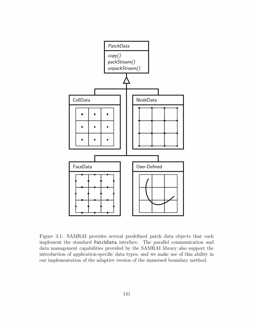
PSfrag replacements

PatchData

copy()

packStream()

unpackStream()

CellData NodeData

FaceData User-Defined

Figure 3.1: SAMRAI provides several predefined patch data objects that eachimplement the standard PatchData interface. The parallel communication anddata management capabilities provided by the SAMRAI library also support theintroduction of application-specific data types, and we make use of this ability inour implementation of the adaptive version of the immersed boundary method.

141

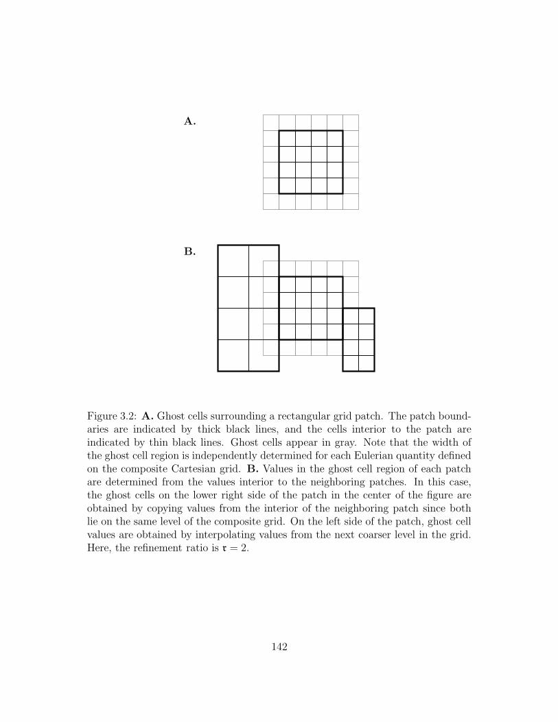
PSfrag replacements

A.

B.

Figure 3.2: A. Ghost cells surrounding a rectangular grid patch. The patch bound-aries are indicated by thick black lines, and the cells interior to the patch areindicated by thin black lines. Ghost cells appear in gray. Note that the width ofthe ghost cell region is independently determined for each Eulerian quantity definedon the composite Cartesian grid. B. Values in the ghost cell region of each patchare determined from the values interior to the neighboring patches. In this case,the ghost cells on the lower right side of the patch in the center of the figure areobtained by copying values from the interior of the neighboring patch since bothlie on the same level of the composite grid. On the left side of the patch, ghost cellvalues are obtained by interpolating values from the next coarser level in the grid.Here, the refinement ratio is r = 2.

142

an application only use some predetermined collection of data types. Moreover,

this design facilitates the development and deployment of application-specific data

types that may be substantially different from the standard ones provided by the

library.

3.2.2 Parallel communication algorithms, operators, and

schedules

Operations that involve parallel communication can also decomposed into compo-

nents that are independent of the configuration of the patch hierarchy and com-

ponents that are specific to a particular hierarchy configuration. In SAMRAI, a

communication algorithm is an object that describes parallel data transactions in

terms of the variables and operations involved, whereas a communication schedule

is an object that stores and executes the particular interprocess transactions that

are required to perform such operations on a given patch hierarchy. Hence, a com-

munication algorithm provides a configuration-independent description of one or

more operations that require parallel communication to be performed, and a com-

munication schedule provides the means to actually perform such operations. As a

result, communication algorithms generally are initialized once at the beginning of

a computation and are then reused throughout the course of the simulation without

further modification. By contrast, communication schedules must be regenerated

each time that the hierarchy configuration is modified, e.g., following adaptive re-

gridding. Since locally refined grids can become quite complicated during the course

of a simulation, the process of regenerating the schedules required by a particular

143

application can itself be an expensive operation. Consequently, communications

schedules are designed so that they may be reused so long as the configuration of

the patch hierarchy remains unmodified. In the context of the present adaptive

version of the immersed boundary method, we typically regrid the patch hierarchy

only every nregrid ≈ 10 timesteps, and as a result we are able to get significant reuse

out of the generated communication schedules.

There are two kinds of communications algorithms provided by the SAMRAI li-

brary: coarsening algorithms and refinement algorithms. Coarsening algorithms

describe operations that move data from finer levels of the patch hierarchy to

coarser levels, whereas refinement algorithms describe operations that move data

from coarser levels to finer levels. Refinement algorithms also can be used to de-

scribe transactions that move data between patches on the same level (e.g., to set

values in ghost cells), as such operations can be thought of as a special case of re-

finement. Both types of communication algorithms are initialized by specifying the

variables involved in the transaction and the operations that are to be performed

on that specified data. Note that in general, data that is moved from one level

of the patch hierarchy to another cannot be simply copied, but instead must be

either restricted from a finer level to a coarser one or interpolated from a coarser

level to a finer one. In the case of a coarsening algorithm, the coarsening operators

are generally some form of conservative averaging, e.g., either cell centered or face

centered conservative averaging. For a refinement algorithm, the refinement opera-

tors may perform interpolation operations such as linear interpolation or piecewise

linear conservative interpolation. User-defined coarsening and refinement operators

may also be provided.

144

Given any particular patch hierarchy configuration, a communication algorithm

is able to compute the particular parallel data transactions required to perform

the specified operations and store them in a communication schedule. For any

particular algorithm and hierarchy configuration, the set of required transactions

is determined by comparing the patch box regions on the source and destination

levels. Such comparisons must be done in an efficient manner if the construction of

communication schedules is to remain a small fraction of the overall computational

workload2 [80]. The schedules that are generated by a coarsening algorithm for

a particular configuration of the patch hierarchy are called coarsening schedules,

whereas those generated by refinement algorithms are referred to as refinement

schedules. Again, note that although communication schedules must be regener-

ated each time that the patch hierarchy is modified, they may be reused between

regridding operations, when the hierarchy configuration remains static.

3.2.3 Parallel computing on grid patches

To make the foregoing notions more concrete, we present here example code3 that

evaluates in parallel a cell centered approximation to the Laplacian of a cell centered

quantity, ui,j,k, on each grid patch on a specified level of the patch hierarchy. More

precisely, for each grid cell (i, j, k) on a particular level of the patch hierarchy, we

2The most easily implemented algorithms for performing such operations are quadratic in thenumber of compared patch boxes. Since the number of patches that comprise the composite gridtends to grow with the size of the problem and with the number of processors, more complexalgorithms are required to avoid the situation where the construction of communication schedulesbecomes a dominate cost of an adaptive computation.

3Extensive comments are provided in the example code in an attempt to make it understand-able for those readers unfamiliar with C++ or FORTRAN syntax.

145

compute

fi,j,k = (Lu)i,j,k (3.3)

using the uniform grid definition of (Lu)i,j,k given by equation (2.29). In the exam-

ple code, the ghost cell values of u that lie on the “coarse side” of the coarse-fine

interface are obtained by linearly interpolating data defined on the next coarser level

of the patch hierarchy. It is important to note that the resulting finite difference

approximation to the Laplacian is different from the one described in Section 2.4.2.

However, it should be emphasized that our purpose here is not to document our

actual implementation of the composite grid finite difference approximation to the

Laplacian, which does indeed compute the approximation described in Section 2.4.2.

Instead, it is to give the reader a sense of the basic structure of that implementa-

tion. Moreover, the basic form of the following code is similar to that of much of

our implementation of the adaptive version of the immersed boundary method, in-

cluding the implementations of the interpolation and finite difference operators, the

explicit Godunov procedure outlined in Section 2.3.7, the multilevel linear solvers

described below in Section 3.4, and even the discrete interaction equations, i.e.,

equations (2.52)–(2.54) and (2.69).

Setting the ghost cell values

The following example code evaluates fi,j,k = (Lu)i,j,k on each patch on the specified

level of the patch hierarchy, where the particular level number is specified by the

integer variable level_num. The first step in doing so involves setting the ghost

cell values for the patch data that corresponds to u. This must be done on each

146

patch on level level_num.

On every patch, there are precisely two types of ghost cells: ghost cells that

intersect the interiors of neighboring patches on the same level, and ghost cells that

lie on the coarse side of the coarse-fine interface. In the following code, when a

ghost cell overlaps the interior of some patch in the same level of the patch hierar-

chy, the value of u in that ghost cell is provided by simply copying data from the

interior of that neighboring patch. Otherwise, when a ghost cell lies on the coarse

side of the coarse-fine interface, the value of u in that ghost cell is determined

by linearly interpolating data from the next coarser level in the patch hierarchy,

i.e., level level_num-1. (Again, we emphasize that the resulting discretization at

the coarse-fine interface in this sample code is different from the one employed in

our actual implementation of the composite grid finite difference approximation to

the Laplace operator.) Note that since the patches on each level are distributed

amongst the available processors, these operations in general require interprocess

communication. In SAMRAI, such parallel communication is performed via stan-

dard MPI routines, and conveniently, these MPI function calls are hidden from the

application developer.

In the following code, note that integer value u_idx is a so-called patch data

descriptor index that indicates the identity of the patch data that corresponds

to the variable u. Similarly, the integer value f_idx indicates which patch data

corresponds to f . Also note that NDIM is an integer value that determines the

number of spatial dimensions. It is set at compile time by a preprocessor directive,

thereby allowing much (but not all) of the code to be “dimensionally independent.”

147

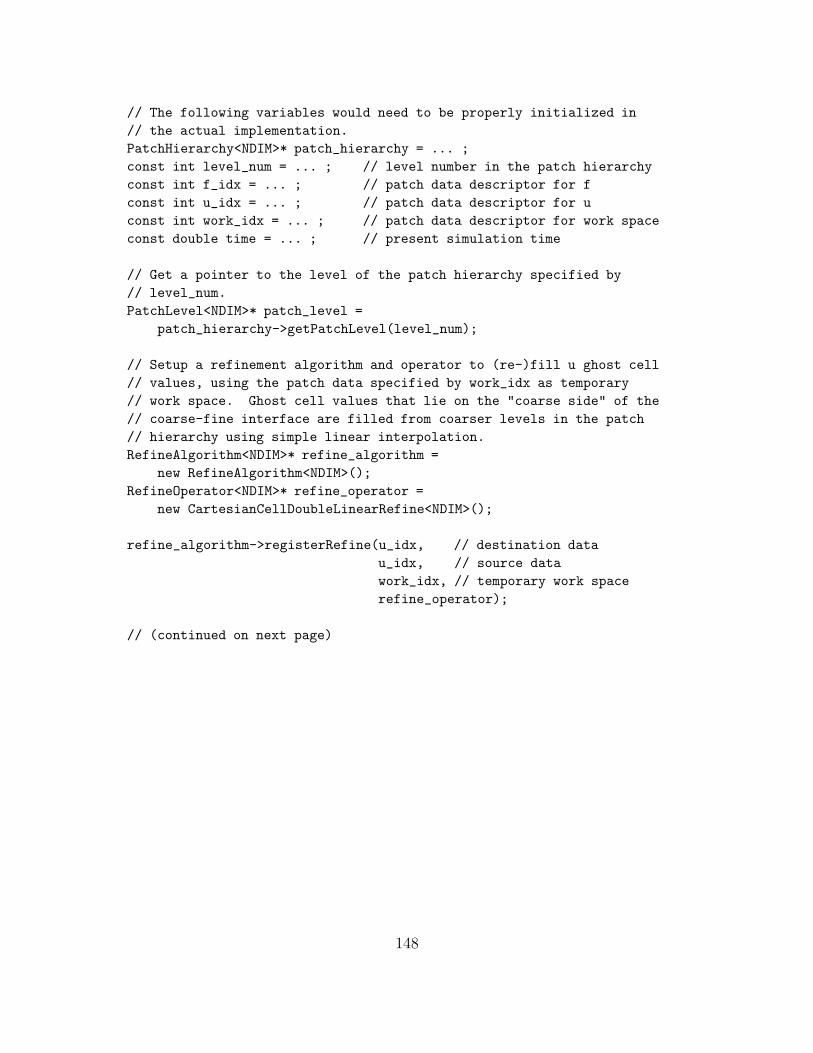
// The following variables would need to be properly initialized in

// the actual implementation.

PatchHierarchy<NDIM>* patch_hierarchy = ... ;

const int level_num = ... ; // level number in the patch hierarchy

const int f_idx = ... ; // patch data descriptor for f

const int u_idx = ... ; // patch data descriptor for u

const int work_idx = ... ; // patch data descriptor for work space

const double time = ... ; // present simulation time

// Get a pointer to the level of the patch hierarchy specified by

// level_num.

PatchLevel<NDIM>* patch_level =

patch_hierarchy->getPatchLevel(level_num);

// Setup a refinement algorithm and operator to (re-)fill u ghost cell

// values, using the patch data specified by work_idx as temporary

// work space. Ghost cell values that lie on the "coarse side" of the

// coarse-fine interface are filled from coarser levels in the patch

// hierarchy using simple linear interpolation.

RefineAlgorithm<NDIM>* refine_algorithm =

new RefineAlgorithm<NDIM>();

RefineOperator<NDIM>* refine_operator =

new CartesianCellDoubleLinearRefine<NDIM>();

refine_algorithm->registerRefine(u_idx, // destination data

u_idx, // source data

work_idx, // temporary work space

refine_operator);

// (continued on next page)

148

// Create a reusable refinement schedule that performs the following

// operations:

//

// (1) linearly interpolate data from the next coarser level of the

// patch hierarchy to those ghost cells that lie on the "coarse

// side" of the coarse-fine interface, and

// (2) copy data from the interiors of the patches on the specified

// level of the patch hierarchy to the remaining ghost cells on

// that same level.

//

// Note that this refinement schedule may be reused so long as the

// patch hierarchy configuration remains unchanged.

RefineSchedule<NDIM>* refine_schedule =

refine_algorithm->createSchedule(patch_level,

level_num-1,

patch_hierarchy);

// Fill the values of u in all ghost cells on the patch level.

//

// Note that the simulation time must be specified here since

// refinement schedules can perform interpolation in time as well as

// space.

refine_schedule->fillData(time);

// Compute the discrete Laplacian on each (local) patch on the

// specified level of the patch hierarchy.

for (PatchLevel<NDIM>::Iterator p(patch_level); p; p++)

Patch<NDIM>* patch = patch_level->getPatch(p());

// See below for discussion of the following syntax.

CellData<NDIM,double>* f_data =

dynamic_cast< CellData<NDIM,double>* >(

patch->getPatchData(f_idx));

CellData<NDIM,double>* u_data =

dynamic_cast< CellData<NDIM,double>* >(

patch->getPatchData(u_idx));

laplace(f_data, u_data, patch); // (see below)

149

After some (intentionally incomplete) preliminary variable declarations, the

foregoing code creates and configures RefineAlgorithm and RefineOperator ob-

jects that define the hierarchy-independent form of the interprocess communication

and data interpolation that must occur to set the values of u in the ghost cell region.

Recall that such objects in general may be used throughout a simulation without fur-

ther modification. Next, the RefineAlgorithm is used to create a RefineSchedule

object. This communication schedule records the particular parallel data transac-

tions that must occur to set the ghost cell values of u for a particular configuration

of the patch hierarchy. Since communication schedule objects define operations

that are specific to a given hierarchy configuration, they must be regenerated each

time the hierarchy configuration changes, although they can be reused so long as

the hierarchy remains unmodified. After the RefineSchedule is created, it is im-

mediately used to set the values of u in the ghost cell region via the invocation of its

fillData() member function. After the call to fillData() completes, no further

parallel communication is required to compute fi,j,k = (Lu)i,j,k on each patch in

the level.

Next, on each process, the code iterates over the local patches in the patch

level (i.e., each parallel process only loops over the patches that have been assigned

to that processor) and obtains pointers to the local NDIM-dimensional CellData

objects that correspond to f and u. (Recall that NDIM indicates the number of

spatial dimensions and is set at compile time.) These pointers are obtained on

each patch from the corresponding Patch object. In particular, the code passes the

patch data descriptor indices to the getPatchData() member function provided by

the Patch class to retrieve pointers to the appropriate patch data objects. These

150

patch data pointers, along with a pointer to the patch object itself, are then passed

on to the function laplace() that is defined below.

(Note that in the foregoing example code, the syntax required to set the values

of f_data and u_data is complicated by the fact that the function getPatchData()

provided by the Patch class does not return pointers to CellData objects. Rather, it

returns pointers to the abstract patch data base class, i.e., pointers to objects of type

PatchData. This is done to allow for the easy specification of user-defined patch

data types that are not provided by the SAMRAI library. However, one consequence

of this design is that a downcast4 (expressed here as a dynamic_cast<>) must be

performed to obtain a CellData* from the value returned by the getPatchData()

member function. In actual applications, is is possible to largely avoid explicitly

downcasting pointers by using a “smart” pointer class provided by the SAMRAI

library that automatically performs such casts when possible. We avoid the use

of such smart pointers in the presentation of this example since, except in a few

instances, doing so reduces the complexity of the syntax of the code.)

Computing (Lu)i,j,k on each patch on the level

Once the ghost values have been set, the evaluation of fi,j,k = (Lu)i,j,k can proceed

in parallel. Each patch may be processed independently of the other patches on

the level, and on any particular patch, very little information is required about the

4A downcast is an operation whereby a pointer to a base class, such as a PatchData*, isconverted to a pointer to a derived class, such as a CellData*. In general, such casting operationsshould be done with some care, since there are typically several different derived classes associatedwith any particular base class. In developing SAMRAI-based applications, however, it is generallya simple matter to ensure that the patch data associated with a particular descriptor indexcorresponds to the anticipated patch data type.

151

geometry of the patch and essentially no information is required as to the relation-

ship between the patch and the rest of the hierarchy5. In particular, evaluating the

finite difference approximation on the patch requires that we determine:

1. the grid spacing on the patch;

2. the extents of the box region occupied by the patch; and

3. the widths of the ghost cell regions for the patch data that defines f and u.

This information is accessible via the Patch object and the CellData objects that

correspond to f and u. The following code retrieves this information, obtains

pointers to the actual data corresponding to f and u, and then calls a low-level

FORTRAN routine that actually computes fi,j,k = (Lu)i,j,k on the patch.

5Note that operations that employ a specialized treatment at the coarse-fine interface typicallydo require some additional information about the relationship between a particular patch and therest of the patch hierarchy. In particular, such operations typically require that a data structurebe provided to indicate where the coarse-fine interface is actually located.

152

// Compute f = div grad u on the specified patch using standard

// second order accurate finite differences.

void laplace(

CellData<NDIM,double>* f_data,

CellData<NDIM,double>* u_data,

Patch<NDIM>* patch)

// Determine the grid spacing on the patch. Note that the grid

// spacing is an NDIM-dimensional array and is not assumed to

// be isotropic.

CartesianPatchGeometry<NDIM>* pgeom =

dynamic_cast< CartesianPatchGeometry<NDIM>* >(

patch->getPatchGeometry());

const double* const dx = pgeom->getDx();

// Determine the region occupied by this patch.

const Box<NDIM>& patch_box = patch->getBox();

// Get pointers to the actual data that corresponds to f and u,

// and then determine the widths of the ghost cell regions for

// each quantity.

double* const f = f_data->getPointer();

const double* const u = u_data->getPointer();

const int f_ghosts = (f_data->getGhostCellWidth()).max();

const int u_ghosts = (u_data->getGhostCellWidth()).max();

// Call a FORTRAN routine to actually evaluate f = div grad u.

ctoclaplace_(

f, f_ghosts,

u, u_ghosts,

patch_box.lower(0), patch_box.upper(0),

#if (NDIM > 1)

patch_box.lower(1), patch_box.upper(1),

#if (NDIM > 2)

patch_box.lower(2), patch_box.upper(2),

#endif

#endif

dx);

return;

153

The implementation of the function laplace() first determines the grid spacing,

dx, and the box that defines the region6 occupied by the patch, patch_box. Both

are specified, either directly or indirectly, through the interface provided by the

Patch object. The code then obtains pointers to the actual data that defines f

and u on the patch and determines the widths of the ghost cell regions for both

quantities. Note that for simplicity, the code assumes that the ghost cell region

widths are uniform, i.e., that the width of the ghost cell region is the same in each

coordinate direction, although f_data and u_data are not assumed to have the

same ghost cell region widths. (For instance, for the present operation to be well-

defined, f is not required to have any ghost cells at all, whereas the patch data

associated with u is required to have at least a single layer of ghost cells surrounding

the interior of each patch.)

The actual data corresponding to f on the patch interior and ghost cell region,

to which we obtain a pointer in the foregoing via f_data->getPointer(), corre-

sponds to a contiguous column-major (FORTRAN-style) array of double precision

values. In three spatial dimensions, the extents of the data accessible through f are

expressed in pseudocode as

f(patch_box.lower(0)-f_ghosts:patch_box.upper(0)+f_ghosts,

patch_box.lower(1)-f_ghosts:patch_box.upper(1)+f_ghosts,

patch_box.lower(2)-f_ghosts:patch_box.upper(2)+f_ghosts)

The data that corresponds to u is similarly defined.

6The lower extents of the region occupied by the patch are specified by the lower() memberfunction provided by the Box class, whereas the upper extents are specified by the upper()

function. Both functions return cell centered indices that correspond to the particular level of thepatch hierarchy to which the patch belongs.

154

Since the actual code that evaluates numerical operations on individual grid

patches must be able to handle data defined on essentially arbitrary boxes, we have

found that it is convenient to implement such operations as simple FORTRAN rou-

tines. In particular, FORTRAN provides extremely simple syntax for “reshaping”

contiguous arrays of data, as is demonstrated in the following code where we finally

provide numerical operations to evaluate fi,j,k = (Lu)i,j,k on a single patch. Note

that this is the only part of this example that is fundamentally dependent on the

number of spatial dimensions.

155

ccccccccccccccccccccccccccccccccccccccccccccccccccccccccccccccccccccccccc

c Computes f = div grad u.

c

c Uses the seven point stencil to compute the cell centered Laplacian

c of a cell centered variable u in three spatial dimensions.

ccccccccccccccccccccccccccccccccccccccccccccccccccccccccccccccccccccccccc

c

subroutine ctoclaplace(

& f,f_ghosts,

& u,u_ghosts,

& i_lower,i_upper,

& j_lower,j_upper,

& k_lower,k_upper,

& dx)

c

implicit none

c

c Input.

c

integer i_lower,i_upper

integer j_lower,j_upper

integer k_lower,k_upper

integer f_ghosts,u_ghosts

double precision u(i_lower-u_ghosts:i_upper+u_ghosts,

& j_lower-u_ghosts:j_upper+u_ghosts,

& k_lower-u_ghosts:k_upper+u_ghosts)

double precision dx(0:2)

c

c Output.

c

double precision f(i_lower-f_ghosts:i_upper+f_ghosts,

& j_lower-f_ghosts:j_upper+f_ghosts,

& k_lower-f_ghosts:k_upper+f_ghosts)

c

c Local variables.

c

integer i,j,k

double precision i_fac,j_fac,k_fac

156

c

c Compute the finite difference approximation to the Laplacian of u.

c

i_fac = 1.d0/(dx(0)**2.d0)

j_fac = 1.d0/(dx(1)**2.d0)

k_fac = 1.d0/(dx(2)**2.d0)

do k = k_lower,k_upper

do j = j_lower,j_upper

do i = i_lower,i_upper

f(i,j,k) =

& i_fac*(u(i-1,j,k)+u(i+1,j,k)-2.d0*u(i,j,k))+

& j_fac*(u(i,j-1,k)+u(i,j+1,k)-2.d0*u(i,j,k))+

& k_fac*(u(i,j,k-1)+u(i,j,k+1)-2.d0*u(i,j,k))

enddo

enddo

enddo

c

return

end

c

157

3.3 Managing the distributed curvilinear mesh

So far, we have described how SAMRAI can be used to manage and communi-

cate data defined on the composite Cartesian grid. In this section, we turn our

attention to the management of data defined on the distributed curvilinear mesh.

To perform the operations required to implement the immersed boundary method,

we again make use of the SAMRAI framework, but here we do so in conjunc-

tion with parallel data structures provided by the PETSc (Portable, Extensible

Toolkit for Scientific Computation) library which is developed at the Mathematics

and Computer Science Division at Argonne National Laboratory [8, 7, 9]. One of

the original goals of the PETSc project was to provide a framework for develop-

ing high-performance parallel scientific applications that make use of unstructured

grids, and we utilize these capabilities to store and communicate data defined on

the distributed curvilinear mesh and to perform computations involving that data.

(Note that although the curvilinear meshes that appear in Chapter 2 are essen-

tially logically Cartesian structured grids, we feel that the fiber structure of the

model of the heart and great vessels employed in Chapter 4 and described in Ap-

pendix A is most easily treated as an unstructured grid, and we have designed our

implementation of the immersed boundary method accordingly.)

In the implementation, each of the Lagrangian quantities defined on the curvi-

linear mesh (e.g., the curvilinear force density, F(·, ·, ·), or the configuration of the

(visco-)elastic structure, X(·, ·, ·)) is stored in a separate PETSc VecMPI distributed-

parallel vector object7. Each curvilinear mesh node has a corresponding entry (or

7Although it is written largely in the C programming language, PETSc employs an object-oriented style similar to that found in many C++-based software libraries.

158

set of entries in the case of a vector valued quantity) in each of the parallel vector

objects. Recall from Section 3.1 that the nodes of the curvilinear mesh are dis-

tributed across the available processors so that each mesh node is assigned to the

same processor as is assigned the Cartesian grid cell in which that mesh node is

embedded, i.e., mesh node (q, r, s) is assigned to the same processor as is assigned

the Cartesian grid patch on level `max that contains the cell (i, j, k) that satisfies

X(q, r, s) ∈ c`max(i, j, k).

Since each quantity defined on the curvilinear mesh is stored as a PETSc vector,

linear operations that are defined on the curvilinear mesh can be expressed in terms

of one of the parallel sparse matrix classes provided by PETSc, e.g., MatMPIAIJ or

MatMPIBAIJ. For instance, in the computations described in Chapter 2, the discrete

curvilinear force density is determined by evaluating a finite difference approxima-

tion to ∂2

∂s2X at the nodes of the curvilinear mesh. A finite difference approximation

to ∂2

∂s2 can easily be described by a PETSc matrix, and once such a matrix object is

initialized, it is a simple matter to compute in parallel the curvilinear force density

on the curvilinear mesh. In particular, given a PETSc matrix L that encodes the

finite difference approximation to ∂2

∂s2 and PETSc vectors X and F that respectively

correspond to the Lagrangian quantities X and F, the discrete curvilinear force

density may be computed via the simple expression MatMult(L,X,F). It is only

slightly more complicated to evaluate in parallel nonlinear force density mappings,

such as those described in Appendix A that specify the elastic forces generated by

deformation to the model heart, since in such cases, the only operations that require

parallel communication typically can be expressed as matrix-vector products.

In addition to evaluating the curvilinear elastic force density, which is a “purely

159

Lagrangian” computation, we must also be able to interpolate the velocity from

the Cartesian grid to the curvilinear mesh and spread the force density from the

curvilinear mesh to the Cartesian grid. This is done by evaluating the discrete

Lagrangian-Eulerian interaction equations (i.e., in the uniform grid case, equations

(2.52)–(2.54) and (2.69)). Like the “purely Eulerian” computations discussed in

Section 3.2, velocity interpolation and force spreading can be performed by evalu-

ating the interaction equations on each local patch in parallel, and like the purely

Eulerian computations, performing these operations within a particular patch re-

quires not only data defined in the patch interior but also values defined within a

ghost cell region surrounding the patch interior. In particular, in the case of velocity

interpolation, the Eulerian velocity, u, must be provided in a properly sized ghost

cell region, whereas in the case of force spreading, the curvilinear force density,

F, must be locally accessible both for the nodes that are located within the patch

interior and for the nodes that are embedded within a ghost cell region.

When velocity interpolation is performed via a regularized delta function with

a support of d meshwidths in each coordinate direction, the support of the delta

function centered about any of the curvilinear mesh nodes within a particular patch

can extend beyond the patch boundary by at most d2

grid cells in any coordinate di-

rection. Thus, interpolating the Cartesian cell centered velocity, u, to any location

within a particular patch requires that a b d2c cell wide ghost cell region be provided

for the patch data associated with u. In particular, should a smaller ghost cell re-

gion be provided, note that it will not be possible to use the specified delta function

to interpolate the values provided by the patch data to an arbitrary location in the

patch interior. Of course, the needed data could be provided by some other means

160

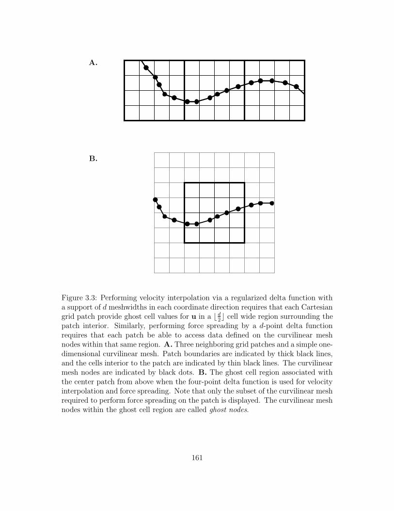
PSfrag replacements

A.

B.

Figure 3.3: Performing velocity interpolation via a regularized delta function witha support of d meshwidths in each coordinate direction requires that each Cartesiangrid patch provide ghost cell values for u in a b d

2c cell wide region surrounding the

patch interior. Similarly, performing force spreading by a d-point delta functionrequires that each patch be able to access data defined on the curvilinear meshnodes within that same region. A. Three neighboring grid patches and a simple one-dimensional curvilinear mesh. Patch boundaries are indicated by thick black lines,and the cells interior to the patch are indicated by thin black lines. The curvilinearmesh nodes are indicated by black dots. B. The ghost cell region associated withthe center patch from above when the four-point delta function is used for velocityinterpolation and force spreading. Note that only the subset of the curvilinear meshrequired to perform force spreading on the patch is displayed. The curvilinear meshnodes within the ghost cell region are called ghost nodes.

161

(e.g., by explicit parallel communication); however, it is convenient to be able to

perform such operations in terms of the local data associated with each patch. Sim-

ilarly, when the same delta function is employed to spread the force density from

the curvilinear mesh to the Cartesian grid, the collection of curvilinear mesh nodes

that can possibly impart some amount of force to the interior of a particular patch

includes not only the mesh nodes that lie within the patch interior but also most8 of

the nodes that lie within the b d2c cell wide ghost cell region surrounding the patch

interior. (See Figure 3.3.)

Supplying the Cartesian ghost cell values required to compute the interpolated

velocity at each curvilinear mesh node requires only that the ghost cell region

associated with the cell centered velocity, u, be at least b d2c cells wide. Since

SAMRAI provides support for arbitrarily sized ghost cell regions, this is easily

accomplished. In a similar manner, ensuring that all of the nodal values of the

curvilinear force density that are required to evaluate the Cartesian force density

within a given patch are accessible on the processor to which that patch is assigned

requires that curvilinear ghost node values be provided on each processor. Once

the identities of the ghost nodes are determined on each processor, facilities for

accessing such ghost node values are provided by the “ghosted” version of the

PETSc VecMPI parallel vector object.

To efficiently determine which of the curvilinear mesh nodes must be provided

as ghost nodes, we introduce some additional Eulerian patch data that is stored

only on the finest level of the patch hierarchy. In particular, for each Cartesian

8When d is even, any curvilinear mesh nodes that are located between the outermost boundaryof the ghost cell region and the outermost “ring” of ghost cell centers cannot impart any force tothe centers of the Cartesian cells that lie in the patch interior.

162

grid cell (i, j, k) on level `max, we explicitly store the set of curvilinear mesh nodes

embedded in that cell, i.e., we maintain for each (i, j, k) the set

Qi,j,k = (q, r, s) : X(q, r, s) ∈ c`max(i, j, k). (3.4)

To store this data on the composite Cartesian grid, we introduce a version of the

standard SAMRAI IndexData patch data type that has been specialized through

template instantiation and class inheritance. For each Cartesian grid cell (i, j, k)

that contains one or more curvilinear mesh nodes, this new patch data type main-

tains data corresponding to the set Qi,j,k, whereas no data is allocated for those

cells that do not contain any curvilinear mesh nodes. (Although we do not discuss

this issue further in the present work, this new patch data type also maintains in-

formation regarding the connectivity of the curvilinear mesh, i.e., it provides a local

portion of a distributed “link table” that indicates which nodes in the curvilinear

mesh are connected by elastic links.) Although this application-specific data type

is not a part of the SAMRAI library, the parallel communication and data man-

agement facilities provided by SAMRAI are designed so that they can be used with

such application-specific data types without modification. In particular, we can use

a SAMRAI RefineAlgorithm to generate a RefineSchedule to fill the ghost cell

values of Q on each patch on level `max, thereby allowing us to determine the set of

curvilinear mesh nodes (including curvilinear mesh ghost nodes) that are required

to spread F(·, ·, ·) to the interior cells of any particular patch in the level.

It may appear that the set of curvilinear coordinate indices associated with

a particular Cartesian grid cell, Qi,j,k, is information that would rapidly become

163

useless, since each node of the curvilinear mesh is constantly in motion. Recall,

however, that the computed velocity, u, and the timestep size, ∆t, must satisfy a

CFL condition of the form

∆t ≤ C min`∈0...`max

h`/ max(i,j,k)∈

level `

(

|uni,j,k|, |vn

i,j,k|, |wni,j,k|

)

, (3.5)

and that in practice, we typically have that C 1. Consequently, in a given

timestep, each curvilinear mesh node may move at most C fractional meshwidths

per timestep in any coordinate direction. As long as Q is updated every b1/Cc

timesteps, then even if the value of Qi,j,k does not indicate the indices of the curvi-

linear mesh nodes that are presently within cell (i, j, k), it at least indicates which

curvilinear mesh nodes are no more than one Cartesian meshwidth away from cell

(i, j, k). (Recall that we also must adaptively regrid the patch hierarchy every

b1/Cc timesteps to ensure that the curvilinear mesh does not “escape” the finest

level of the locally refined Cartesian grid. Thus, it suffices to update the value of

Q as part of the regridding process; see below.) It is not difficult to modify the

algorithms that make use of Q to take this small amount of “uncertainty” into

account.

The Eulerian quantity Qi,j,k is also used in redistributing the curvilinear mesh

when the hierarchy configuration changes. Each time that the patch hierarchy is

adaptively regridded, the distribution of the curvilinear mesh nodes across the pro-

cessors must be updated to correspond to the newly generated set of Cartesian grid

patches. The new configuration of the distributed curvilinear mesh can be deter-

mined from Q, but only if the value of Qi,j,k is properly reset in each cell before the

164

patch hierarchy is regenerated9. In particular, before the composite grid is recon-

structed, we must ensure that Q accounts for the actual, present configuration of

the curvilinear mesh (i.e., we must eliminate the “uncertainty” mentioned above).

Since Qi,j,k is data defined on the composite Cartesian grid, its parallel redistribu-

tion is automatically handled by the SAMRAI library. Once the patch hierarchy

has been reconfigured, the portion of the distributed curvilinear mesh that is as-

signed to a particular processor is determined from the values of Q defined on each

of the local Cartesian grid patches on level `max. Using this information, we can

then create a PETSc VecScatter object which is then used to “scatter” each La-

grangian quantity from the old configuration of the distributed curvilinear mesh to

the newly defined data distribution.

Before concluding this section, we note that PETSc provides extensive support

for the solution of linear and nonlinear systems of equations. As we describe in the

following section, we already make some use of this functionality to solve systems

of linear equations defined on the composite Cartesian grid. (Note that this is

possible as a result of a SAMRAI-PETSc interface that allows SAMRAI data to

be treated like a PETSc Vec object.) We have noted previously that the explicit

treatment of the Lagrangian equations of motion that is employed in the present

version of the immersed boundary method results in a severe restriction on the

size of the largest stable timestep. Such restrictions can be overcome by making

use of an implicit version of the immersed boundary method [77, 43]; however, to

date, it appears that an implicit version of the immersed boundary method that is

9In principle, it is possible to reset Q after the patch hierarchy is regenerated; however, do-ing so would require us to re-implement functionality similar to that provided by the SAMRAIRefineAlgorithm and RefineSchedule objects.

165

suitable for large-scale simulation has not been developed. Addressing this issue is

likely to be crucial to obtaining highly resolved simulation results by any version of

the immersed boundary method, adaptive or otherwise. Since we already employ

PETSc data structures to describe the quantities defined on the curvilinear mesh,

it should not be overly difficult to further exploit the functionality provided by

PETSc to solve the systems of linear and nonlinear equations that appear in implicit

treatments of the Lagrangian equations of motion. Although this work has not yet

been done, we anticipate being able to use the present computational framework as

a platform for developing new implicit versions of the immersed boundary method.

3.4 Parallel linear solvers

We finally turn our attention to the algorithms we employ to solve systems of

linear equations defined on the composite grid. For instance, recall from Chapter 2

that during timestep n of the present version of the immersed boundary method,

the updated velocity, un+1, is defined to be the approximate projection of the

intermediate velocity, u∗. Computing this projection requires that we first solve a

Poisson problem of the form

Lϕ = D · u∗. (3.6)

Then, un+1 is given by

un+1 = u∗ −Gϕ. (3.7)

Composite grid systems of equations also must be solved to compute the time-

centered advection velocity, uADV, the intermediate velocities, u∗ and u∗, and

166

the updated pressure, pn+ 12 . (Recall that the remaining velocity computed during

timestep n, namely the “auxiliary” MAC velocity, uMAC,n+1, is obtained in terms

of the solution to the same Poisson problem that is solved to determine un+1.)

For simplicity, in the present section, we restrict our attention to algorithms for

the solution of the composite grid scalar Poisson problem,

Lu = f. (3.8)

Although we do not specifically consider them here, linear systems of the form

(I − κL)u = f (3.9)

also appear in the description of the adaptive projection method for κ > 0. (Recall

that L is a nonpositive operator, so that for κ ≥ 0, I − κL is a positive operator.)

The algorithms we describe in the present section require no essential modifications

to be deployed in the solution of such problems. Note that the quantities u and f

that appear throughout this section generally should not be taken to be related to

quantities with the same designations that appear elsewhere in the present work.

The same is true of the quantities v, e, and r that are introduced below when we

begin our discussion of the multigrid algorithm in Section 3.4.2.

167

3.4.1 A necessary condition for the solvability of the com-

posite grid Poisson problem

Before we describe the algorithms that we use to solve Poisson problems on the

composite grid, we first briefly address the issue of when it is possible to solve such

systems and outline how one can show that all such problems encountered in the

adaptive version of the immersed boundary method at least satisfy a necessary

condition for solvability.

Since we impose periodic boundary conditions on the physical domain, U , equa-

tion (3.8) is solvable only if f satisfies a discrete analogue of the continuous com-

patibility condition10,∫

U

f dx = 0. (3.10)

In particular, for a uniform grid discretization of U , it is necessary that f satisfy

∑

i,j,k

fi,j,k h3 = 0. (3.11)

In the more general case, when the physical domain, U , is described in terms of a

multilevel composite grid, f must satisfy a similar condition, namely

`max∑

`=0

∑

valid(i,j,k)∈

level `

fi,j,k h3` = 0. (3.12)

Recall that we distinguish between valid and invalid regions of each level of the

10Note that since I − κL is a positive operator for κ ≥ 0, no similar restriction must be placedon f when we solve equations of the form (3.9).

168

composite grid, and that for a cell centered quantity, the valid region of level `

consists of precisely those level ` cells that are not covered by any finer grid cells.

It is not overly difficult to see that each linear system of equations of the form

(3.8) that appears in the adaptive version of the immersed boundary method has

a right-hand-side that satisfies the composite grid compatibility condition, (3.12).

In the numerical scheme, such systems are only encountered when we compute

the projection of a composite grid vector field. As we recall above, computing the

approximate cell centered projection of a cell centered velocity, u∗, requires that

we solve a system of equations of the form

Lϕ = D · u∗. (3.13)

Similarly, to compute the exact MAC projection of a MAC velocity, uMAC,∗, we

must solve a linear system of the form

LϕMAC = Df→c · uMAC,∗. (3.14)

Regardless of the particular values of u∗ and uMAC,∗, it can be shown that the

right-hand-sides of both of the foregoing systems of equations satisfy (3.12). To

do so, we first recall that we define the composite grid cell centered divergence in

terms of the MAC divergence. In particular, D · u∗ is defined by

(D · u∗)i,j,k = (Df→c · Ac→fu∗)i,j,k. (3.15)

Thus, the cell centered divergence of a cell centered vector field is equal to the MAC

169

divergence of a related MAC vector field. Consequently, to demonstrate that each

linear system of the form (3.8) that appears in the present version of the immersed

boundary method possesses a right-hand-side that satisfies (3.12), it suffices to show

that`max∑

`=0

∑

valid(i,j,k)∈

level `

(

Df→c · uMAC)

i,j,kh3

` = 0 (3.16)

for any MAC vector field, uMAC. Conveniently, it is well-known that both the

uniform and composite grid MAC divergence operators (trivially) satisfy a discrete

version of the divergence theorem [55]. In the uniform grid case, the “discrete MAC

divergence theorem” allows us to write

∑

i,j,k

(

Df→c · uMAC)

i,j,kh3 = (3.17)

=

(

∑

j,k

uMACN+ 1

2,j,k− uMAC

− 12,j,k

+∑

i,k

vMACi,N+ 1

2,k− vMAC

i,− 12,k

+∑

i,j

wMACi,j,N+ 1

2− wMAC

i,j,− 12

)

h2,

where uMAC = (uMAC, vMAC, wMAC), and where N is the number of grid cells in

each coordinate direction. Since U is periodic, however, it is clear from (3.17) that

for any value of uMAC,

∑

i,j,k

(

Df→c · uMAC)

i,j,kh3 = 0. (3.18)

The composite grid version of (3.17) is analogous, although the notation is some-

what more cumbersome and so we omit the details. The result, however, is that

Df→c ·uMAC does indeed satisfy (3.16), independent of the particular value of uMAC.

170

We note that it is difficult to show (and indeed perhaps has not yet been shown)

that (3.16) is sufficient to ensure the solvability of LϕMAC = Df→c · uMAC on

an arbitrarily composed composite grid. However, in practice, our solvers always

appear able to converge, even for very complicated composite grids.

3.4.2 The basic multigrid algorithm

We begin our discussion of the particular algorithms that we employ to solve sys-

tems of the form

Lu = f (3.19)

by giving a brief overview of the multigrid algorithm for the special case that the

physical domain, U , is described by a uniform grid. Note that we also make use of

this uniform grid version of the multigrid algorithm in the multilevel case, which we

address below in Section 3.4.3. (More thorough presentations of multigrid appear

in, e.g., [22, 15]. See also, e.g., [17, 70] and the references therein for more details on

the convergence properties and algorithmic complexity of multigrid and multigrid-

like methods.)

The basic multigrid algorithm is heuristically motivated as follows: If u is the

solution to (3.19) and if v is an approximation to u, then the error in the approxi-

mation is the quantity e defined by

e = u− v. (3.20)

Thus, given any approximate solution, if the error is known, then the actual solution

171

is trivially obtained by computing u = v+e. Of course, so long as the true solution

is unknown, so is the error. In fact, e is itself the solution to a related system of

linear equations, namely

Le = r, (3.21)

where r = f − Lv is the residual. Nonetheless, if we were able to obtain an

approximation to the error, say e, then we might hope that we could use e to

improve our approximation to the true solution by computing

v ← v + e. (3.22)

In essence, multigrid is an efficient algorithm for determining such an approximation

to the error. The key to its efficiency is that when basic iterative methods (such as

Gauss-Seidel or damped11 Jacobi iterations) are employed to solve systems of the

form (3.19) or (3.21), only a small number of iterations are required to damp the

high-frequency, oscillatory components of the error in the approximate solution12.

In particular, a small number of Gauss-Seidel or damped Jacobi iterations yields

an approximation to the true solution whose error, e = u− v, is “smooth” on the

original uniform discretization of U . (Because of this smoothing behavior, such

basic iterative methods are frequently referred to as smoothers in the multigrid

literature.) On a coarser discretization of U , however, this same error generally

appears “less smooth,” and hence on a coarser grid, we can again use an inexpensive

11Note that the use of undamped Jacobi can lead to a divergent multigrid algorithm. For themodel problem Lu = f on a uniform grid, a damping factor of ω = 2

3 is optimal; see [22].12Unfortunately, the remaining low-frequency error modes are much more slowly eliminated

from the approximate solution by such basic iterative methods, hence the need for a more complexalgorithm.

172

smoother to rapidly eliminate the high-frequency components in that coarsened

error. Thus, to obtain an approximation to the error on the original fine grid,

the multigrid algorithm restricts the residual, r = f − Lv, from the original fine

grid to a coarser discretization of U . Next, a small number of Gauss-Seidel or

damped Jacobi iterations are used to solve approximately the residual equation,

(3.21), on this coarser grid, thereby obtaining an approximation to the true error

on that grid. This approximation to the error, which we denote by e, is then

prolonged from the coarser grid back to the original fine grid. This interpolation of

the approximation to the coarse grid error is subsequently used to update v on the

original fine grid, although note that the approximation is improved by this process

only when appropriate choices are made for each of the components of the overall

algorithm (e.g., the restriction and prolongation operators and the smoother).

In the foregoing, we have informally described a two-grid version of the multigrid

algorithm. In practice, the algorithm is performed recursively on increasingly coarse

discretizations of the physical domain. (In fact, for scalar Poisson problems of the

form (3.19), the coarsest grid typically consists of only a single grid cell!) Concisely

presenting this recursive version of the algorithm requires that we introduce some

additional notation. Let Uh denote a uniform discretization of the physical domain

with a uniform grid spacing h. Thus, Uh and U2h are both discretizations of U ,

but the grid spacing employed by U 2h is a factor of two coarser than that of Uh.

Let h0 denote the grid spacing on the original discretization of U , so that U h0 is

the computational domain on which we wish to solve Lu = f . For a particular grid

spacing h, let uh, vh, fh, rh, and eh denote quantities that are defined on Uh, and

let Lh denote the finite difference approximation to the Laplacian that corresponds

173

to Uh. Finally, let Ih→2h denote a coarsening operator that restricts quantities from

Uh to U2h, and similarly let I2h→h denote an interpolation operator that prolongs

quantities from U 2h to Uh. The recursive version of the basic multigrid V-cycle

algorithm is then given by:

174

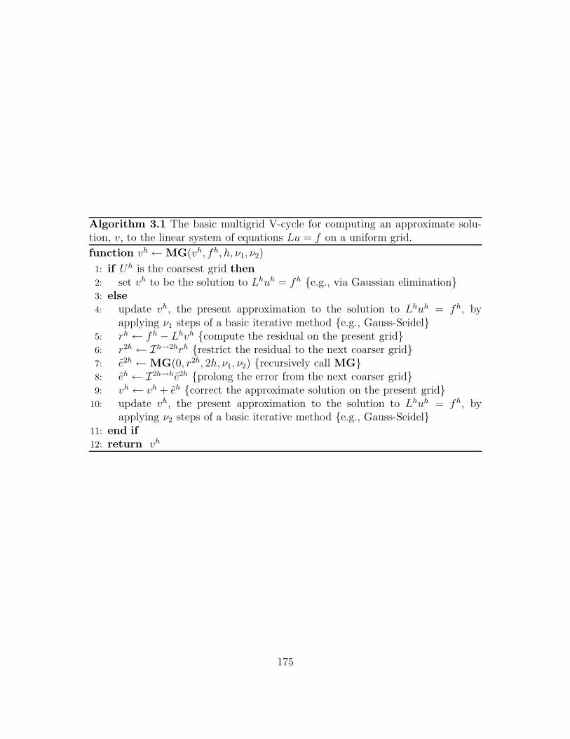
Algorithm 3.1 The basic multigrid V-cycle for computing an approximate solu-tion, v, to the linear system of equations Lu = f on a uniform grid.

function vh ←MG(vh, fh, h, ν1, ν2)

1: if Uh is the coarsest grid then

2: set vh to be the solution to Lhuh = fh e.g., via Gaussian elimination3: else

4: update vh, the present approximation to the solution to Lhuh = fh, byapplying ν1 steps of a basic iterative method e.g., Gauss-Seidel

5: rh ← fh − Lhvh compute the residual on the present grid6: r2h ← Ih→2hrh restrict the residual to the next coarser grid7: e2h ←MG(0, r2h, 2h, ν1, ν2) recursively call MG8: eh ← I2h→he2h prolong the error from the next coarser grid9: vh ← vh + eh correct the approximate solution on the present grid

10: update vh, the present approximation to the solution to Lhuh = fh, byapplying ν2 steps of a basic iterative method e.g., Gauss-Seidel

11: end if

12: return vh

175

Note that common choices for ν1 and ν2 in practice are (ν1, ν2) = (1, 1) or (0, 1).

Although a single V-cycle multigrid iteration is typically not sufficient to obtain

a good approximation to the true solution, at least for the model problem considered

in the present section, an accurate approximation to u may be obtained on U h0 by

performing a relatively small number (e.g., 10) of V-cycles, for instance via:

1: rh0 ← fh0 − Lh0vh0 compute the residual

2: while ‖rh0‖ ≥ εtol do

3: eh0 ←MG(0, rh0, h0, ν1, ν2) approximate the error

4: vh0 ← vh0 + eh0 update the approximate solution

5: rh0 ← fh0 − Lh0vh0 recompute the residual

6: end while

Faster convergence to the true solution may be obtained by using a slightly more

complicated V-cycle algorithm known as full multigrid. In either case, however, the

number of V-cycles required to yield a specified reduction in the error is independent

of h0, i.e., is independent of the grid spacing on the discretization of U on which

we wish to solve Lu = f . Moreover, the total work required by the algorithm is

O(Nd0 ), where d is the number of spatial dimensions and N0 is the number of grid

cells in each coordinate direction on Uh0 . Consequently, multigrid is considered

an (asymptotically) optimal solution algorithm, since it computes a solution by

performing only O(1) operations per grid cell.

Our implementation of the adaptive version of the immersed boundary method

makes use of the parallel multigrid solvers that are developed as part of the hypre

project at the Center for Applied Scientific Computing at Lawrence Livermore

176

National Laboratory [35, 26]. Presently, hypre provides a suite of multigrid solvers

that are designed for use with large problems on massively parallel computers. The

particular algorithm that we currently make most frequent use of is known as PFMG

and is described in, e.g., [6, 25]. Although PFMG is somewhat more complicated

than the algorithm we have sketched here, both employ the same fundamental ideas.

3.4.3 FAC: A composite grid version of the multigrid algo-

rithm

In the previous section, we outlined an approach to solving linear systems of equa-

tions on uniform grids, i.e., the multigrid algorithm. Of course, to implement the

adaptive scheme, we must be able to solve such systems on hierarchically composed

locally refined grids. We do so by making use of a composite grid generalization of

multigrid known as the fast adaptive composite grid method, or simply FAC. Like

multigrid, for which the number of iterations required to yield a specified reduction

in the error is independent of the uniform grid spacing, the convergence rate of

FAC is independent of the number of levels in the composite grid. In particular,

the number of FAC iterations required to reduce an initial error by a given factor

does not grow as more levels are added to the composite grid. Thus, like multigrid,

FAC is considered to be an (asymptotically) optimal algorithm. (More detailed

descriptions of the development, convergence properties, and algorithmic complex-

ity of FAC can be found in, e.g., [44, 46, 45]. See also [37, 38] for a more recent,

asynchronous version of FAC known as AFACx.)

To describe the FAC algorithm, we again introduce some additional notation.

177

As usual, we number the levels of the composite grid by ` = 0, . . . , `max, where ` = 0

indicates the coarsest level and ` = `max indicates the finest. In the description of

the algorithm, it is convenient to make use of level variables, i.e., variables that are

independently defined on each level of the patch hierarchy. In particular, unlike a

composite grid variable, the values of a level variable in the invalid region of a level

are not assumed to be related in any way to values defined on other levels of the

composite grid. In the following, let r` and e` denote level variables defined on level

`. Let I`→(`−1) denote a coarsening operator that restricts quantities defined on

level ` to the portion of the next coarser level that is covered by level ` (i.e., that

coarsens data on level ` onto the invalid region of level `−1). Similarly, let I (`−1)→`

denote an interpolation operator that prolongs quantities defined on the coarser

level `−1 to the finer level `. Finally, let Uh` denote the uniform grid discretization

of the region of the physical domain that is geometrically covered by level `, and

let Lh` denote the appropriate uniform grid approximation to the Laplacian on the

interior of Uh` . In particular, note that Lh` does not employ a modified difference

stencil at the coarse-fine interface; in the algorithm, the treatment at the coarse-

fine interface is facilitated by the manner in which the ghost cell values are defined.

The basic FAC algorithm is then given by:

178

Algorithm 3.2 The main FAC solver loop for computing an approximate solution,v, to the linear system of equations Lu = f on a composite grid.

1: synchronize v and f on the composite grid2: r ← f − Lv compute the composite grid residual3: while ‖r‖ ≥ εtol do

4: e← 0 (re-)initialize e on each level of the composite grid5: FACsweep(e, r, `max, ν, ν1, ν2)6: v ← v + e7: synchronize v on the composite grid8: r ← f − Lv compute the composite grid residual9: end while

Algorithm 3.3 The composite grid generalization of the multigrid V-cycle forcomputing an approximate solution, e, to the linear system of equations Le = r oneach level of a composite grid.

function FACsweep(e, r, `, ν, ν1, ν2)

1: if ` = 0 then

2: e` ←MG(0, r`, h0, ν1, ν2) perform a single iteration of the V-cycle multigridalgorithm on the coarsest level of the hierarchy; note that until this point inthe sweep, e` = 0

3: else

4: r`−1 ← I`→(`−1)r` restrict the residual to the next coarser level; note thatat this point in the sweep, e` = 0

5: FACsweep(e, r, `− 1, ν, ν1, ν2) recursively call FACsweep6: e` ← I(`−1)→`e`−1 prolong the error from the next coarser level to provide

an initial approximation to the error on this level; note that until this pointin the sweep, e` = 0

7: smoothError(e, r, `, ν) see below8: end if

179

Note that we typically employ the values (ν, ν1, ν2) = (2, 0, 2).

As we have described it, the FAC algorithm consists of two components:

1. an outer loop that iteratively corrects the approximation to the solution to

Lu = f on the composite grid (Algorithm 3.2); and

2. an inner loop that makes two passes through the levels of the composite grid,

a “downward” pass from finer levels to coarser levels and an “upward” pass

from coarser levels back to finer ones (Algorithm 3.3).

On the downward pass of the inner loop, Algorithm 3.3 simply ensures that the

residual is appropriately initialized on each level of the hierarchy. (In fact, this is

not required so long as the composite grid residual is properly initialized when it

is passed to the FACsweeep routine.) During this downward sweep, note that

the approximation to the error, e, is zero on each level of the hierarchy. Once the

coarsest level is reached, a single multigrid V-cycle is performed to obtain an initial

approximation to the error on that level. In this context, the uniform grid multigrid

algorithm is referred to as the bottom solver 13. Finally, during the upward sweep,

an approximation to the level ` error is first obtained by prolonging the error from

the next coarser level, level `− 1. This initial approximate error is then smoothed

on level ` by the smoothError function that is defined below.

It is important to note that as Algorithm 3.3 cycles through the levels of the

composite grid, the results are retained in the level variables e` that are (inde-

pendently) defined on each level of the hierarchy. Once FACsweep completes its

13This terminology is traditional but slightly misleading in the present context, since the singlemultigrid V-cycle employed on level ` = 0 is generally insufficient to actually solve Lh0 e0 = r0.

180

downward and upward passes through the patch hierarchy, this collection of level

variables is used to update the composite grid approximation to the solution in the

main FAC solver loop.

An implementation of the foregoing FAC algorithm, including the outer solver

loop and the inner FAC V-cycle, is provided by the SAMRAI library. In our

applications of the algorithm, we employ conservative averaging for the restriction

operator, I`→(`−1), and simple linear interpolation for the prolongation operator,

I(`−1)→`. (Note that conservative linear interpolation is not required; moreover, its

use decreases the convergence rate of the solver.)

Although the SAMRAI framework provides a version of the smoothError func-

tion that is suitable for use in the solution to cell centered Poisson problems, we

provide our own implementation that seems to yield slightly better performance.

Before we state our version of smoothError, let us define e`patch and r`

patch to be the

restrictions of e` and r` to a single level ` grid patch. Similarly, let Lh`

patch denote the

restriction of Lh` to a level ` patch. (Recall that Lh` is the uniform grid definition

of the Laplacian that is associated with the portion of the domain associated with

Uh`, and that the coarse-fine discretization is implicitly handled by the definition

of ghost cell values.) Our version of the smoothError function is then given by:

181

Algorithm 3.4 The grid patch-based smoother employed in the inner FAC V-cycle.

function smoothError(e, r, `, ν)

1: for i = 1 to ν by 1 do

2: if ` > 0 then

3: for all coarse-fine interface ghost cells on level ` do

4: compute the value of e` via the appropriate version of (2.120) see Sec-tion 2.4.2

5: end for

6: end if

7: fill all remaining ghost cells values of e`

8: for all patches on level ` do

9: update e`patch on the patch via a single symmetric Gauss-Seidel iteration

for the local system of equations Lh`

patche`patch = r`

patch note that boundaryconditions are provided by the values in the ghost cell region of the patch

10: end for

11: end for

182

Note that the symmetric version of Gauss-Seidel, which is also known as SSOR(1),

is discussed in, e.g., [10, 22]. (Somewhat surprisingly, in the present context, a

single symmetric Gauss-Seidel sweep on each patch is more effective than two non-

symmetric Gauss-Seidel sweeps, even though the overall FAC algorithm does not

define a symmetric operator.)

The foregoing definition of smoothError yields a “level smoother” that is ex-

tremely similar to a parallel multigrid smoother that is commonly referred to as

processor block Gauss-Seidel [1]. In that algorithm, the physical domain is decom-

posed into several subdomains that are distributed across the available processors.

Gauss-Seidel iterations are then performed simultaneously on each processor on

the local portion of the discretization. Despite its name, however, processor block

Gauss-Seidel is not a true Gauss-Seidel algorithm; instead, it is a block Jacobi al-

gorithm that locally applies Gauss-Seidel on each subdomain. The only difference

between a more typical processor block Gauss-Seidel algorithm and Algorithm 3.4

is that processor block Gauss-Seidel generally employs only a single subdomain

per processor, whereas in Algorithm 3.4, there are in general multiple decoupled

subdomains (i.e., grid patches) per processor.

It is important to note that for some problems, processor block Gauss-Seidel

has irregular convergence properties that depend on the parallel distribution of

the computational domain. Moreover, when processor block Gauss-Seidel is used

as a multigrid smoother, it can sometimes yield a divergent algorithm [1]. (This

is a result of the overall block Jacobi-like character of the algorithm.) Despite

these potential pitfalls, at least for the scalar Poisson problems encountered in the

present work, we have found that FAC converges in a steady and reliable manner

183

when we use the smoother defined by Algorithm 3.4 in conjunction with PFMG as

a multigrid bottom solver.

3.4.4 Implementation issues

Although FAC is often effective as a standalone linear solver, Algorithm 3.3 also

may be used as a preconditioner for a Krylov subspace method such as the well-

known Generalized Minimum Residual (GMRES) method. In our applications of

the adaptive immersed boundary method, we generally use FAC as a preconditioner

rather than as a solver, since we have found that doing so tends to yield slightly

better performance, although the improvement is rather modest. The present cell

centered version of the FAC algorithm can be paired with any Krylov method that

is suitable for the solution of nonsymmetric14 systems of linear equations, including

GMRES and the Bi-Conjugate Gradient Stabilized (Bi-CGSTAB) method. (An

excellent and freely available reference that includes descriptions of most of the

commonly used Krylov methods, along with basic iterative methods and precondi-

tioners, is [10]. See also, e.g., [22, 76].)

For systems of equations of the form

(I − κL)u = f, (3.23)

14Note that although our composite grid discretization of the Laplacian is symmetric, a sym-metric version of the cell centered FAC algorithm has apparently not yet been developed. Despitethis difficulty, the present version of FAC can generally be used with the conjugate gradient (CG)method, as the preconditioned operator is apparently only “mildly” nonsymmetric. We do notuse CG, however, as in practice we seem to obtain better performance from methods such asGMRES.

184

with κ > 0, we employ the FAC-preconditioned GMRES method. In the present

version of the immersed boundary method, systems of this form result from the im-

plicit treatment of the viscous terms in the momentum equation, and in such cases

κ = O(∆t). Consequently, these systems generally are quite well conditioned. In

particular, for the values of κ that we typically encounter in our present appli-

cations, systems of the form (3.23) can be solved to a relative error tolerance of

at least 1.0e-8 within approximately three preconditioned GMRES iterations, and

frequently the solver converges after only a single preconditioned iteration. In ei-

ther case, the rate of convergence is sufficiently rapid to avoid the use a restarted

version of GMRES. (Note that each preconditioned GMRES iteration employs a

single matrix-vector product and a single application of the FAC preconditioner,

but that the amount of storage required by GMRES grows linearly with the number

of iterations.)

To solve systems of the form

Lu = f, (3.24)

we employ the FAC-preconditioned Bi-CGSTAB method, and for such problems,

Bi-CGSTAB generally convergences to a relative error tolerance of 1.0e-8 or higher

within approximately six iterations. (Note that each preconditioned Bi-CGSTAB

iteration employs two matrix-vector multiplications and two FAC sweeps, i.e., twice

the number per iteration than GMRES. Unlike GMRES, however, the amount of

storage required by Bi-CGSTAB is independent of the number of iterations.)

Rather than developing our own implementations of these preconditioned Krylov

subspace methods, we instead make use of the suite of Krylov solvers provided by

185

the PETSc library. This is facilitated by a SAMRAI-PETSc interface, whereby

SAMRAI data defined on the (SAMRAI-maintained) composite grid may be passed

to a PETSc solver as if it were a native PETSc vector. In fact, SAMRAI data

that is “wrapped” in a PETSc-compatible interface in this manner may be passed

as an argument to any PETSc function that uses only the standard vector space

operations (e.g., scalar multiplication and vector-vector operations such as addition,

subtraction, and the dot product). Besides these standard vector space operations,

Krylov solvers only require routines to evaluate matrix-vector products (i.e., in the

present context, routines that evaluate f ← Lv or f ← (I − κL)v) and routines

that apply the preconditioner (i.e., here, FACsweep). Although these operations

are largely implemented in terms of SAMRAI objects, supplying such routines to

the PETSc solvers requires only an extremely modest amount of “glue” code to

interface the SAMRAI-based implementation to the PETSc solver. As a result

of the flexible design of both SAMRAI and PETSc, we consequently are able to

harness the widely used and extensively tested PETSc solvers within a largely

SAMRAI-based application by providing only a small amount of additional code.

186

Chapter 4

Simulating the blood-muscle-valve

mechanics of the heart

In the previous chapters, we have introduced an adaptive, formally second order ac-

curate version of the immersed boundary method, demonstrated that this method

actually converges at a second order rate when it is used to simulate the interac-

tion of a viscous incompressible fluid and a viscoelastic shell, and described the

implementation of this scheme for distributed-memory parallel computers. In the

present chapter, we finally turn our attention to the application of this parallel

and adaptive methodology to Peskin and McQueen’s three-dimensional model of

cardiac mechanics [62, 49, 64, 52, 53]. The implementation of this model requires

a small number of changes to the numerical methods described in Chapter 2, and

we briefly outline the necessary modifications before presenting simulation results.

Before doing so, however, we first summarize those anatomical and physiological

features of the heart and nearby great vessels that are most relevant to our compu-

187

tational results (a more complete discussion of cardiac physiology can be obtained

from any text on medical physiology, e.g., Guyton and Hall [31]). We then briefly

describe the three-dimensional model employed in the present chapter1.

4.1 An overview of cardiac anatomy and physiol-

ogy and the model heart

The heart is a four chambered organ that consists of two pumps, the left and

right sides of the heart, whose respective duties are to pump oxygenated blood

to the tissues of the body and to pump oxygen-depleted blood returned from the

tissues of the body to the lungs, where the blood is reoxygenated. Each side of

the heart is comprised of two chambers, namely an atrium and a ventricle, and

in both cases, the weaker atrium acts as a receiving chamber and as a primer

pump for the more powerful ventricle. The left side of the heart is responsible for

pumping oxygenated blood through the systemic circulation to the tissues of the

body. To accomplish this task, the left ventricle is necessarily thick and muscular.

In comparison, the right ventricle is thin-walled. This is a reflection of the function

of the right side of the heart, which is to return deoxygenated blood to the lungs

and then back to the left atrium, a distance that is considerably shorter than the

length of the systemic circulation. Consequently, the right ventricle is required to

generate pressures that are approximately a sixth of those generated by the left

1To differentiate more clearly the present work from that of Peskin and McQueen, a moredetailed description of the three-dimensional fiber model of the heart and great vessels is postponeduntil Appendix A, which summarizes their work. In particular, note that the initial configurationof the model heart, its valves, and the nearby great vessels is displayed in Figures A.1–A.10.

188

ventricle, despite the fact that for a healthy individual, the left and right sides of

the heart pump approximately the same amount of blood over the cardiac cycle.

On the left side of the heart, the pulmonary veins supply oxygen-enriched blood

from the lungs to the left atrium, whereas the right atrium is filled with blood that

is returned from the tissues of the body by the superior and inferior vena cavae.

On both sides of the heart, blood empties from the atria into the ventricles via

the atrioventricular valves, namely the mitral valve on the left side of the heart

and the tricuspid valve on the right. Both atrioventricular valves are supported

by fans of fibrous chordae tendineae, which in turn insert into papillary muscles

anchored in the ventricular walls and the interventricular septum. In a healthy

heart, the papillary muscles pull on the chordae tendineae during ventricular systole

(i.e., ventricular contraction) to prevent the atrioventricular valves from bulging

backwards into the atria.

During systole, blood pours out of the ventricles, through the arterial valves,

and into the great arteries. On the left side of the heart, the left ventricle ejects

blood through the aortic valve into the ascending aorta, whereas the right ventricle

ejects through the pulmonic valve into the main pulmonary artery. Unlike the

atrioventricular valves, both arterial valves are self-supporting. The arterial valve

openings are also much smaller than those of the atrioventricular valves, which

results in higher ejection velocities and more severe mechanical stresses.

The model of the heart and great vessels described in Appendix A and employed

in the present chapter includes representations of all of the major features of the

heart and nearby great vessels, including the four chambers of the heart, i.e., the left

and right ventricles and atria; the two atrioventricular (inflow) valves, including the

189

supporting fans of chordae tendineae and papillary muscles; the two arterial (out-

flow) valves; the veins that return blood to the atria, i.e., the pulmonary veins and

the superior and inferior vena cavae; and finally the major arteries that carry the

blood ejected by the ventricles, i.e., the ascending aorta and the main pulmonary

artery. Each of these structures is modeled as a system of elastic fibers: in the case

of the valves, the fibers mainly correspond to passive collagen fibers; in the great

vessels, they correspond to smooth muscle tissue; and in the myocardium, they

correspond to active muscle fibers that possess time-dependent contractile proper-

ties. A brief discussion of the elastic properties of these structures is provided in

Appendix A, but the main result is that most of the forces generated by the elastic-

ity of the model heart may be computed in the manner described in Section 2.3.4,

although the fiber tension is determined differently. In particular, the fiber tension

varies both temporally (to simulate active, contractile muscle) and spatially (to

simulate the waves of muscle activation and deactivation that propagate through

the heart). Nonetheless, implementing the elastic properties specified by the model

requires no major changes to the numerical scheme presented in Chapter 2.

In the model, the blood is treated as a viscous incompressible fluid with uniform

mass density, ρ = 1.0 (g/cm3), and uniform dynamic viscosity, µ = 0.04 (g/cm sec).

The fiber structure of the heart and great vessels is taken to be incompressible and

neutrally buoyant, and the viscous properties of the heart are assumed to be the

same as those of the blood. The region surrounding the model heart is taken to be

filled with fluid that possesses the same uniform mass density and viscosity as the

blood. This is not completely unrealistic since in the body, the heart is surrounded

by the pericardium, which includes a fluid-filled layer that lubricates the heart.

190

Even outside the pericardium, there is tissue that has nontrivial attributes such

as incompressibility, mass density, and viscosity, and the motion of this external

tissue is coupled to that of the heart. To represent the external tissue as fluid with

the same properties as the blood may be a crude approximation, but it is a better

approximation than ignoring the external tissue completely. As before, periodic

boundary conditions are imposed on the physical domain, and the heart and blood

are assumed to be initially at rest, so that u0 ≡ 0. It is important to emphasize that

in the model, the motion of the heart and blood is not specified for t > 0. Instead,

the dynamics are determined during the course of the simulation by solving the

equations of motion for the coupled fluid-structure system.

Before concluding this section, it is important to note that the model does not

include a detailed description of the circulation. Instead, the inflow and outflow

vessels all have blind ends, and fluid sources and sinks are provided to establish

realistic pressure loads on each side of the heart. Implementing this aspect of

the model does necessitate several changes to the previously described numerical

methods, and these modifications are the subject of the following section.

4.2 Connecting the model heart to a model of the

circulation

As we have noted, in the three-dimensional fiber model of the heart used in the

present chapter, the inflow and outflow vessels are not connected to a detailed

model of the circulatory system. Instead, the great vessels (including the ascending

191

aorta, the pulmonary artery, the pulmonary veins, and the superior and inferior

vena cavae) all have hemispherically capped blind ends. Fluid sources and sinks

are supplied in or near these blind ends to establish realistic pressure loads and

thereby simulate connections to the rest of the circulation. A consequence of this,

however, is that it is no longer the case that ∇ · u ≡ 0. Instead, fluid is locally

created or destroyed at a net rate qsrc, so that

∇ · u = qsrc 6≡ 0. (4.1)

It is perhaps not surprising that modifications to the continuous and discretetized

equations of motion are necessitated by the introduction of fluid sources and sinks

that are internal to the physical domain. A derivation of the modified continuous

equations by C. S. Peskin is detailed in Appendix B, and the numerical treatment

of these modified continuous equations is described below in Section 4.2.1, although

in both cases these changes are independent of the particular form of qsrc. We then

briefly describe in Section 4.2.2 the present manner in which qsrc is determined when

the model heart is coupled to the model circulation. For simplicity, we consider here

only the case of a uniform discretization of the Eulerian equations of motion. In

practice, appropriate extensions to the adaptively refined case are straightforward

to implement.

4.2.1 Modifications to the discrete equations of motion

As detailed in Appendix B, the Eulerian equations of motion (i.e., the incompress-

ible Navier-Stokes equations) must be modified when fluid sources and sinks lie

192

within the physical domain, U . The main result of the derivation of the modified

equations is that an additional “friction” term associated with the sources and sinks

must be included in the momentum equation, and that the form of this friction-like

term depends on the manner in which the nonlinear terms of the Navier-Stokes

equations are written. Three equivalent forms of the modified continuous equa-

tions are summarized in Section B.3, but in our numerical methods and simulation

results, we shall make use of only the second of these three alternate forms. In

particular, we make use of the “non-conservative” or “transport” form, (B.34), as

this is the form of the modified equations that most closely resembles the more

standard form of the equations considered in Chapter 2.

Recalling equations (2.1)–(2.5) from Section 2.2, the equations of motion for

the coupled fluid-structure system, modified for the case that there are distributed

fluid sources and sinks within the physical domain, are:

ρ

(

∂u

∂t+ (u · ∇)u

)

+∇p = µ∇2u + f − ρuq+src, (4.2)

∇ · u = qsrc, (4.3)

f(x, t) =

∫

Ω

F(q, r, s, t) δ(x−X(q, r, s, t)) dq dr ds, (4.4)

∂X

∂t(q, r, s, t) = u(X(q, r, s, t), t) (4.5)

=

∫

U

u(x, t) δ(x−X(q, r, s, t)) dx,

F(·, ·, ·, t) = F [X(·, ·, ·, t), t], (4.6)

193

where q+src is defined by

q+src(x, t) =

qsrc(x, t), if qsrc(x, t) ≥ 0,

0, if qsrc(x, t) ≤ 0.(4.7)

It is important to note that the pressure, p, that appears in the foregoing equa-

tions (and throughout the present chapter) is different from the quantity called the

pressure that appears in the derivation of the modified Navier-Stokes equations.

In particular, if we let pB denote the quantity referred to as the pressure in Ap-

pendix B, then pB = p + 13µqsrc. Also, since U is taken to be a periodic box, note

that it is necessary that qsrc satisfy the compatibility condition

∫

U

qsrc(x, t) dx = 0, (4.8)

since, with ∂U denoting the boundary of U with outward unit normal n,

∫

U

qsrc dx =

∫

U

∇ · u dx =

∫

∂U

u · n dS = 0 (4.9)

by the divergence theorem and the periodicity of u. This compatibility condition

essentially requires that the total volume of fluid that enters the physical domain,

U , through fluid sources over any arbitrary interval of time be exactly balanced by

corresponding outflow through fluid sinks during that same time interval. This is

a reflection of the fact that despite the presence of internal fluid sources and sinks,

the fluid is still incompressible.

To treat these modified continuous equations of motion, there are only two major

194

changes that must be made to our original discretization of the original continuous

equations. In particular, our original treatment of the momentum equation must

be altered to account for the friction-like term associated with the fluid sources

that now appears on the right-hand side of (4.2). We also must account for the fact

that ∇ · u = qsrc 6≡ 0 when we project the various intermediate velocity fields. We

briefly outline these changes presently, assuming for simplicity that qsrc(x, t) is an

externally supplied source/sink distribution2.

Modifications to the discretized momentum equation

We first describe our approximations to the additional friction-like term associ-

ated with fluid sources, −ρuq+src, that now appears in the momentum equation.

Approximations to this term must be evaluated twice during each timestep: first,

during the Godunov extrapolation procedure that is employed to determine the

explicit approximation to [(u · ∇)u]n+ 12 ; and second, during the computation of the

intermediate velocities, u∗ and u∗.

When we employ the Godunov procedure described in Section 2.3.7 to extrapo-

late uni,j,k to cell faces, instead of using the source term defined by equation (2.81),

we employ the modified source term

ψni,j,k =

1

ρ

(

(f1)ni,j,k − ρ

(

Af→c1 uMAC

)n

i,j,k

(

q+src

)n

i,j,k− (Gxp)

n− 12

i,j,k

)

, (4.10)

where f = (f1, f2, f3) is the discrete Cartesian elastic force density and Gp =

(Gxp,Gyp,Gzp) is the discrete pressure gradient. Similar formulas yield the appro-

2As we shall discuss in Section 4.2.2, in our simulation results, qsrc is in fact determined duringthe course of the computation.

195

priate source terms for v and w. Note that for qsrc ≡ 0, the modified source term

specified by (4.10) reduces to equation (2.81).

Similarly, during the timestepping procedure described in Section 2.3.6, rather

than solving equation (2.56) to obtain u∗, we instead solve

(I − η2νL)(I − η1νL)u∗ = (I + η3νL)un+ (4.11)

+ ∆t(I + η4νL)

(

−Nn+ 12 +

1

ρ

(

fn+ 12 − ρ

(

Af→cuADV) (

q+src

)n+ 12 −Gpn− 1

2

)

)

,

where uADV is the timestep centered advection velocity that is determined during

the evaluation of the approximation to [(u · ∇)u]n+ 12 . A similar expression replaces

equation (2.62) to determine u∗.

Modifications to the approximate cell centered and exact MAC projec-

tions

Next, the forms of the cell centered and MAC projections must be altered to account

for ∇ · u = qsrc 6≡ 0. In the modified scheme, un+1 is obtained from u∗ during

timestep n by first solving a discrete Poisson problem for ϕ,

Lϕ = D · u∗ − qn+1src ,

and then evaluating

un+1 = u∗ −Gϕ.

For this Poisson problem to be solvable, it is necessary that∑

i,j,k(qsrc)n+1i,j,k = 0, i.e.,

qsrc must satisfy a discrete version of the continuous compatibility condition, (4.8).

196

In the case that qn+1src ≡ 0, this modified projection clearly reduces to the standard

cell centered approximate projection operator defined by equation (2.32) in Chap-

ter 2. Like its more standard counterpart, this modified cell centered projection

is approximate in the sense that un+1 does not satisfy D · un+1 = qn+1src pointwise.

However, so long as u and qsrc are smooth, ‖D ·un+1− qn+1src ‖ → 0 as the Cartesian

grid is refined3. Similar modifications are made to the procedure by which pn+ 12 is

determined from u∗.

Recall that in addition to the cell centered velocity, u, we also maintain a MAC

velocity, uMAC. It is not hard to see that since uMAC,∗ = Ac→fu∗, we may still obtain

uMAC,n+1 from uMAC,∗ in terms of the approximate projection of u∗. In particular, as

before, the solution to the same system of linear equations is used both to determine

un+1 from u∗ and to determine uMAC,n+1 from uMAC,∗. Moreover, the modified MAC

projection is still exact in the sense that(

Df→c · uMAC,n+1)

i,j,k≡ (qsrc)

n+1i,j,k.

Analogously, during timestep n, we obtain the timestep-centered advection ve-

locity, uADV, via the modified Godunov procedure. Similarly to the original scheme

described in Section 2.3.7, we now obtain uADV from uADV,∗ by first solving a dis-

crete Poisson problem,

LϕADV = Df→c · uADV,∗ − qn+ 12

src ,

and then evaluating

uADV = uADV,∗ −Gc→fϕADV.

Again, this operation is exact in the sense that(

Df→c · uADV)

i,j,k≡ (qsrc)

n+ 12

i,j,k .

3In the case of a uniform Cartesian grid, ‖D · un+1 − qn+1src ‖ = O(h2) for smooth u and qsrc.

197

4.2.2 Determining qsrc from a reduced model of the circu-

lation

We now turn our attention the the determination of qsrc. In the present model,

there are a total of five (regularized) point sources and sinks that are positioned

inside the structures of the heart and great vessels. These include two point sources

located near the capped ends of the superior and inferior vena cavae along with a

third source located inside the left atrium, just below the four pulmonary veins.

Corresponding fluid sinks are positioned near the capped ends of the ascending

aorta and the main pulmonary artery. These sources and sinks must remain within

these model structures during the course of the computation; however, the motion

of the fiber structures is itself determined during the course of the simulation and

is not known a priori. Consequently, the position of each point source or sink must

be determined from the time-varying configuration of the model heart. To do so,

five “clouds” of passive marker particles are embedded in the fiber structure of

the heart, one for each source or sink. Each cloud consists of a large number of

markers, and the location of a particular source or sink is taken to be the centroid

of the corresponding marker cloud. The motion of the clouds of marker particles

is determined in precisely the same manner as that of the fiber structure of the

heart (i.e., by numerically integrating the interpolation of the computed Eulerian

velocity field, u; see equations (2.52) and (2.69)). So long as the initial position of

each marker exactly coincides with that of some node of the curvilinear fiber mesh,

the clouds of markers remain exactly embedded within the fiber structure of the

heart throughout the simulation.

198

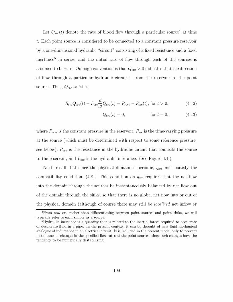
Let Qsrc(t) denote the rate of blood flow through a particular source4 at time

t. Each point source is considered to be connected to a constant pressure reservoir

by a one-dimensional hydraulic “circuit” consisting of a fixed resistance and a fixed

inertance5 in series, and the initial rate of flow through each of the sources is

assumed to be zero. Our sign convention is thatQsrc > 0 indicates that the direction

of flow through a particular hydraulic circuit is from the reservoir to the point

source. Thus, Qsrc satisfies

RsrcQsrc(t) + Lsrcd

dtQsrc(t) = Prsvr − Psrc(t), for t > 0, (4.12)

Qsrc(t) = 0, for t = 0, (4.13)

where Prsvr is the constant pressure in the reservoir, Psrc is the time-varying pressure

at the source (which must be determined with respect to some reference pressure;

see below), Rsrc is the resistance in the hydraulic circuit that connects the source

to the reservoir, and Lsrc is the hydraulic inertance. (See Figure 4.1.)

Next, recall that since the physical domain is periodic, qsrc must satisfy the

compatibility condition, (4.8). This condition on qsrc requires that the net flow

into the domain through the sources be instantaneously balanced by net flow out

of the domain through the sinks, so that there is no global net flow into or out of

the physical domain (although of course there may still be localized net inflow or

4From now on, rather than differentiating between point sources and point sinks, we willtypically refer to each simply as a source.

5Hydraulic inertance is a quantity that is related to the inertial forces required to accelerateor decelerate fluid in a pipe. In the present context, it can be thought of as a fluid mechanicalanalogue of inductance in an electrical circuit. It is included in the present model only to preventinstantaneous changes in the specified flow rates at the point sources, since such changes have thetendency to be numerically destabilizing.

199

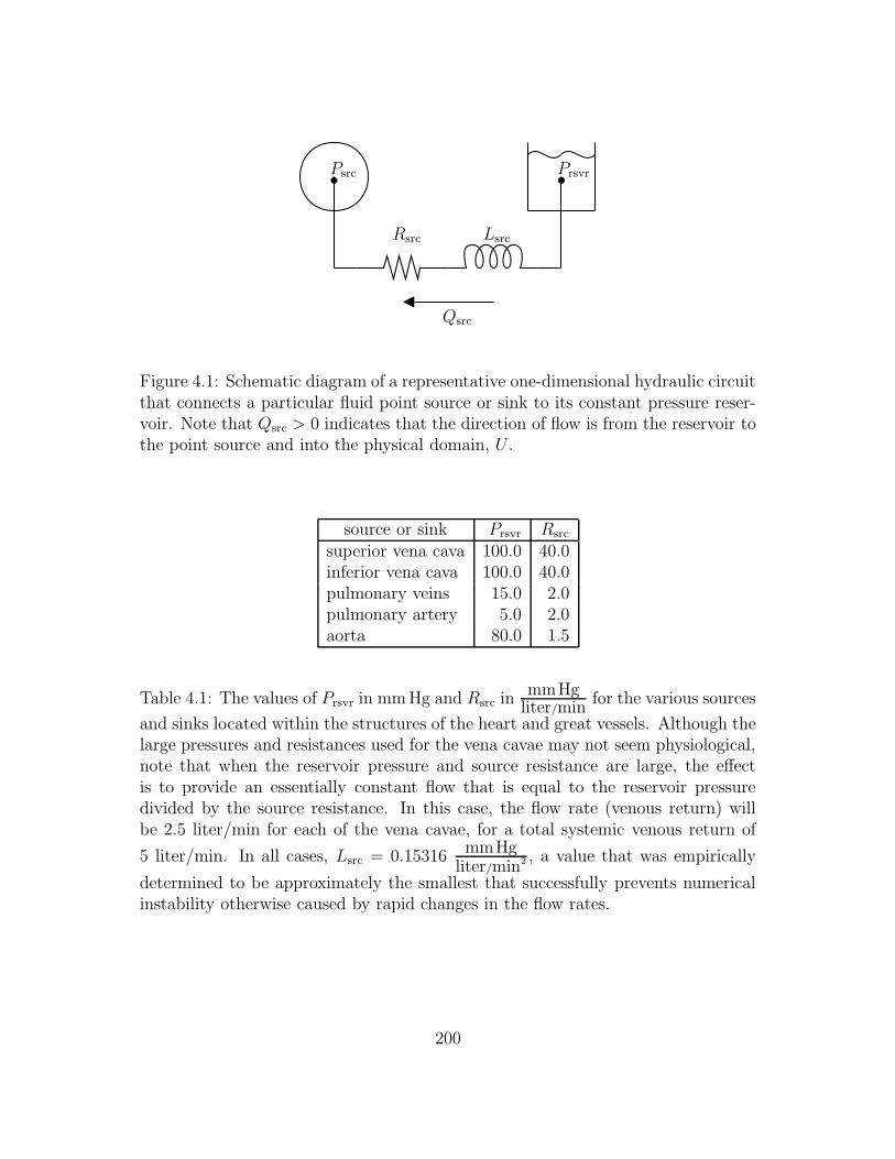
PSfrag replacementsRsrc Lsrc

Qsrc

Psrc Prsvr

Figure 4.1: Schematic diagram of a representative one-dimensional hydraulic circuitthat connects a particular fluid point source or sink to its constant pressure reser-voir. Note that Qsrc > 0 indicates that the direction of flow is from the reservoir tothe point source and into the physical domain, U .

source or sink Prsvr Rsrc

superior vena cava 100.0 40.0inferior vena cava 100.0 40.0pulmonary veins 15.0 2.0pulmonary artery 5.0 2.0aorta 80.0 1.5

Table 4.1: The values of Prsvr in mm Hg and Rsrc inmmHg

liter/minfor the various sources

and sinks located within the structures of the heart and great vessels. Although thelarge pressures and resistances used for the vena cavae may not seem physiological,note that when the reservoir pressure and source resistance are large, the effectis to provide an essentially constant flow that is equal to the reservoir pressuredivided by the source resistance. In this case, the flow rate (venous return) willbe 2.5 liter/min for each of the vena cavae, for a total systemic venous return of

5 liter/min. In all cases, Lsrc = 0.15316mmHg

liter/min2 , a value that was empirically

determined to be approximately the smallest that successfully prevents numericalinstability otherwise caused by rapid changes in the flow rates.

200

outflow). However, in general the rate of blood flow into the heart at the sources

will not be exactly balanced by corresponding outflow at the sinks. For instance,

early in the simulation, the sources in the veins are responsible for filling the heart

with blood. At this point in the computation, however, there is generally little or

no corresponding outflow through the sinks in the arteries. By contrast, later in the

simulation during ventricular ejection, the large volume of blood that is expelled

into the sinks in the arteries is not matched by correspondingly large inflow from

the veins. Consequently, if qsrc is to satisfy (4.8), a compensating source/sink must

be provided to ensure that there is no net change in the fluid volume. It is most

natural to place this additional source/sink away from the structures of the heart

and great vessels. Unlike the sources within the heart and great vessels, which are

modeled as (regularized) point sources, the external source/sink is taken to occupy

a large rectangular volume, V0, that is aligned with the faces of the Cartesian grid

cells. In an attempt to maximize the distance between the heart and the external

source/sink, V0 is placed so that it spans both sides of the periodic boundary that

faces the left and right sides of the heart.

We are now ready to state more precisely the manner in which qsrc is determined.

As there is no initial flow through any of the sources or sinks, q0src ≡ 0. At each

timestep n > 0, we first compute the mean value of the most recent available

pressure (i.e., pn− 12 ) within the external source/sink via

P n0 =

1

vol(V0)

∑

i,j,k∈V0

pn− 1

2i,j,k . (4.14)

This value is taken to be the reference pressure when we determine the pressures

201

at the remaining point sources.

Next, numbering the point sources l = 1, . . . , 5, we determine the present posi-

tion of each internal point source l as the centroid of the appropriate cloud of mark-

ers embedded in the fiber structure of the heart (i.e., essentially from Xn(·, ·, ·)).

Let Xnl denote the position of point source l at time tn. The pressure at each point

source, P nl , is obtained by interpolating the pressure from the Cartesian grid to the

point source locations using a “spread-out” version of the four-point delta function.

In particular, for l = 1, . . . , 5, we compute

P nl =

(

∑

i,j,k

pn− 1

2i,j,k

1

8δIB4h

(

1

2(xi,j,k −Xn

l )

)

h3

)

− P n0 . (4.15)

Having obtained the pressures at each source in reference to P0, the rate of blood

flow at each point source l, denoted Qnl , is then determined via a backward-Euler

discretization of (4.12). The mean rate of flow at the external source/sink is then

given by

Qn0 = − 1

vol(V0)

5∑

l=1

Qnl , (4.16)

so that the net flow rate into the domain through the internal sources is matched

by corresponding outflow at the external source/sink.

Finally, we obtain qnsrc on the Cartesian grid, again using the spread-out version

of the four-point delta function, via

(qsrc)ni,j,k =

5∑

l=1

Qnl

1

8δIB4h

(

1

2(xi,j,k −Xn

l )

)

h3 +

Qn0 , if (i, j, k) ∈ V0,

0, otherwise.(4.17)

202

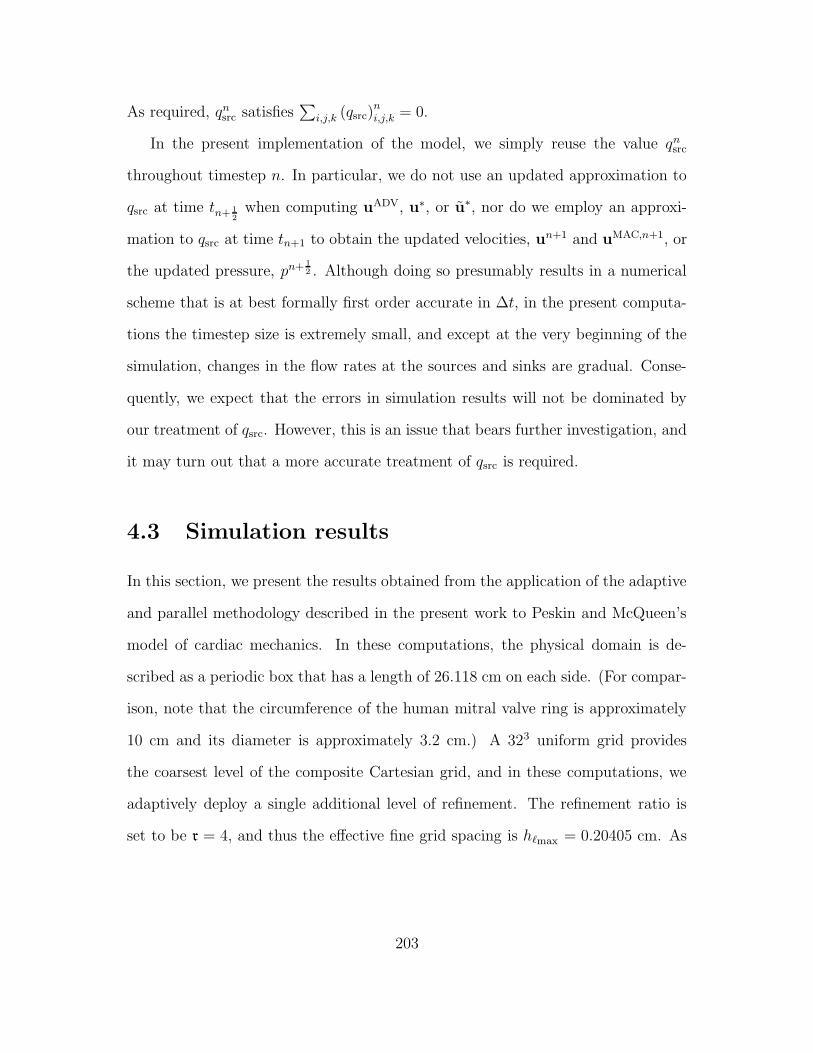
As required, qnsrc satisfies

∑

i,j,k (qsrc)ni,j,k = 0.

In the present implementation of the model, we simply reuse the value qnsrc

throughout timestep n. In particular, we do not use an updated approximation to

qsrc at time tn+ 12

when computing uADV, u∗, or u∗, nor do we employ an approxi-

mation to qsrc at time tn+1 to obtain the updated velocities, un+1 and uMAC,n+1, or

the updated pressure, pn+ 12 . Although doing so presumably results in a numerical

scheme that is at best formally first order accurate in ∆t, in the present computa-

tions the timestep size is extremely small, and except at the very beginning of the

simulation, changes in the flow rates at the sources and sinks are gradual. Conse-

quently, we expect that the errors in simulation results will not be dominated by

our treatment of qsrc. However, this is an issue that bears further investigation, and

it may turn out that a more accurate treatment of qsrc is required.

4.3 Simulation results

In this section, we present the results obtained from the application of the adaptive

and parallel methodology described in the present work to Peskin and McQueen’s

model of cardiac mechanics. In these computations, the physical domain is de-

scribed as a periodic box that has a length of 26.118 cm on each side. (For compar-

ison, note that the circumference of the human mitral valve ring is approximately

10 cm and its diameter is approximately 3.2 cm.) A 323 uniform grid provides

the coarsest level of the composite Cartesian grid, and in these computations, we

adaptively deploy a single additional level of refinement. The refinement ratio is

set to be r = 4, and thus the effective fine grid spacing is h`max = 0.20405 cm. As

203

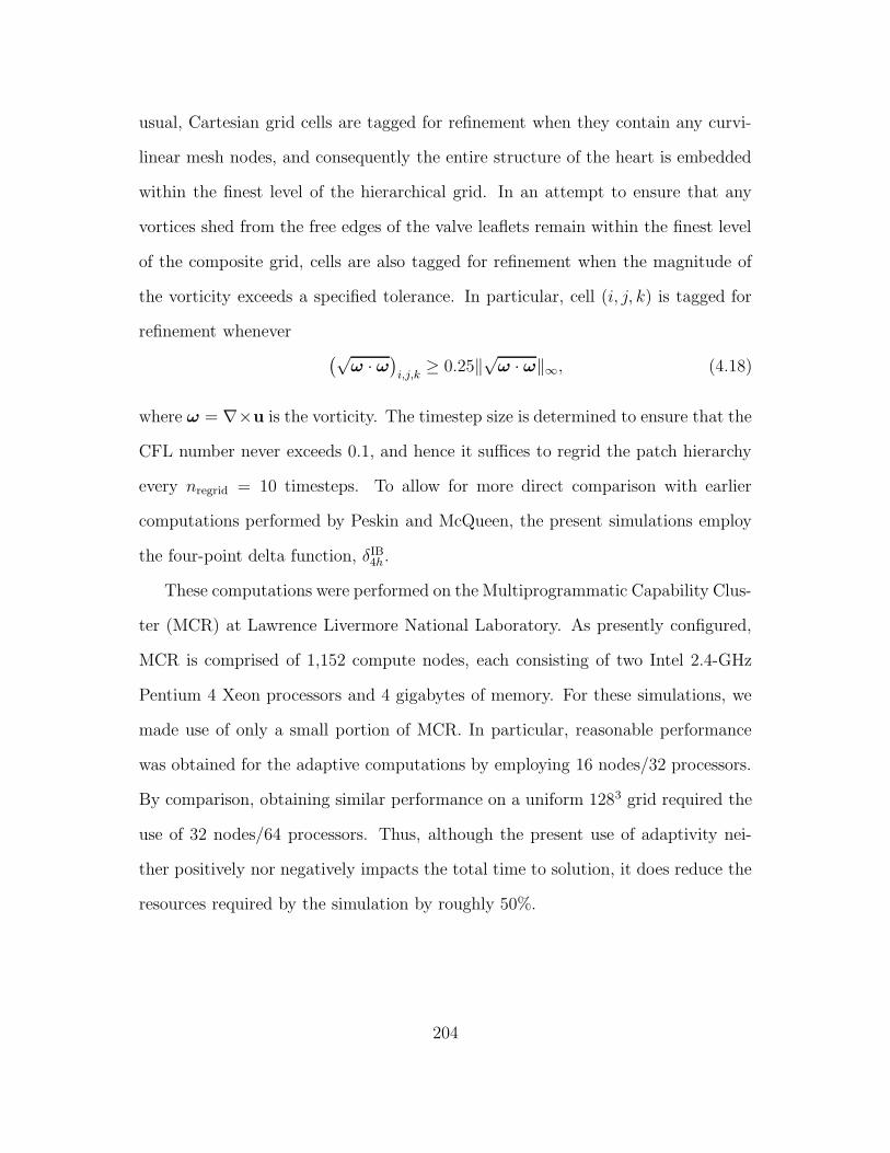
usual, Cartesian grid cells are tagged for refinement when they contain any curvi-

linear mesh nodes, and consequently the entire structure of the heart is embedded

within the finest level of the hierarchical grid. In an attempt to ensure that any

vortices shed from the free edges of the valve leaflets remain within the finest level

of the composite grid, cells are also tagged for refinement when the magnitude of

the vorticity exceeds a specified tolerance. In particular, cell (i, j, k) is tagged for

refinement whenever(√

ω · ω)

i,j,k≥ 0.25‖

√ω · ω‖∞, (4.18)

where ω = ∇×u is the vorticity. The timestep size is determined to ensure that the

CFL number never exceeds 0.1, and hence it suffices to regrid the patch hierarchy

every nregrid = 10 timesteps. To allow for more direct comparison with earlier

computations performed by Peskin and McQueen, the present simulations employ

the four-point delta function, δIB4h.

These computations were performed on the Multiprogrammatic Capability Clus-

ter (MCR) at Lawrence Livermore National Laboratory. As presently configured,

MCR is comprised of 1,152 compute nodes, each consisting of two Intel 2.4-GHz

Pentium 4 Xeon processors and 4 gigabytes of memory. For these simulations, we

made use of only a small portion of MCR. In particular, reasonable performance

was obtained for the adaptive computations by employing 16 nodes/32 processors.

By comparison, obtaining similar performance on a uniform 1283 grid required the

use of 32 nodes/64 processors. Thus, although the present use of adaptivity nei-

ther positively nor negatively impacts the total time to solution, it does reduce the

resources required by the simulation by roughly 50%.

204

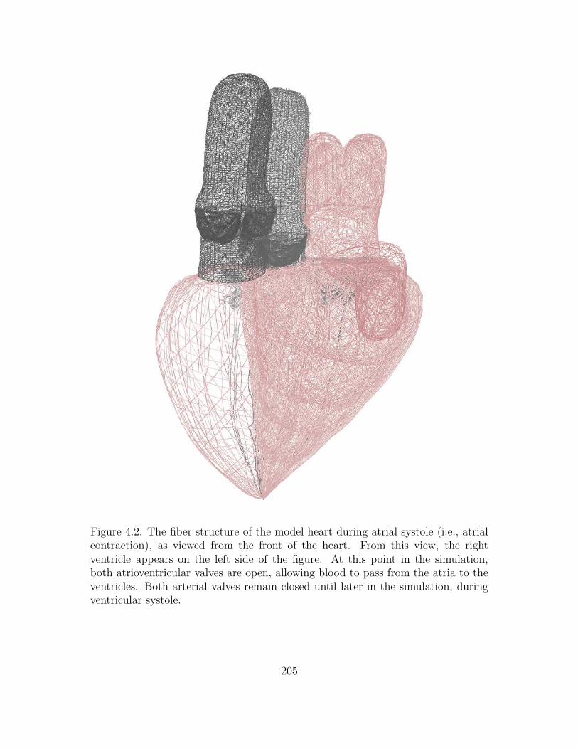
Figure 4.2: The fiber structure of the model heart during atrial systole (i.e., atrialcontraction), as viewed from the front of the heart. From this view, the rightventricle appears on the left side of the figure. At this point in the simulation,both atrioventricular valves are open, allowing blood to pass from the atria to theventricles. Both arterial valves remain closed until later in the simulation, duringventricular systole.

205

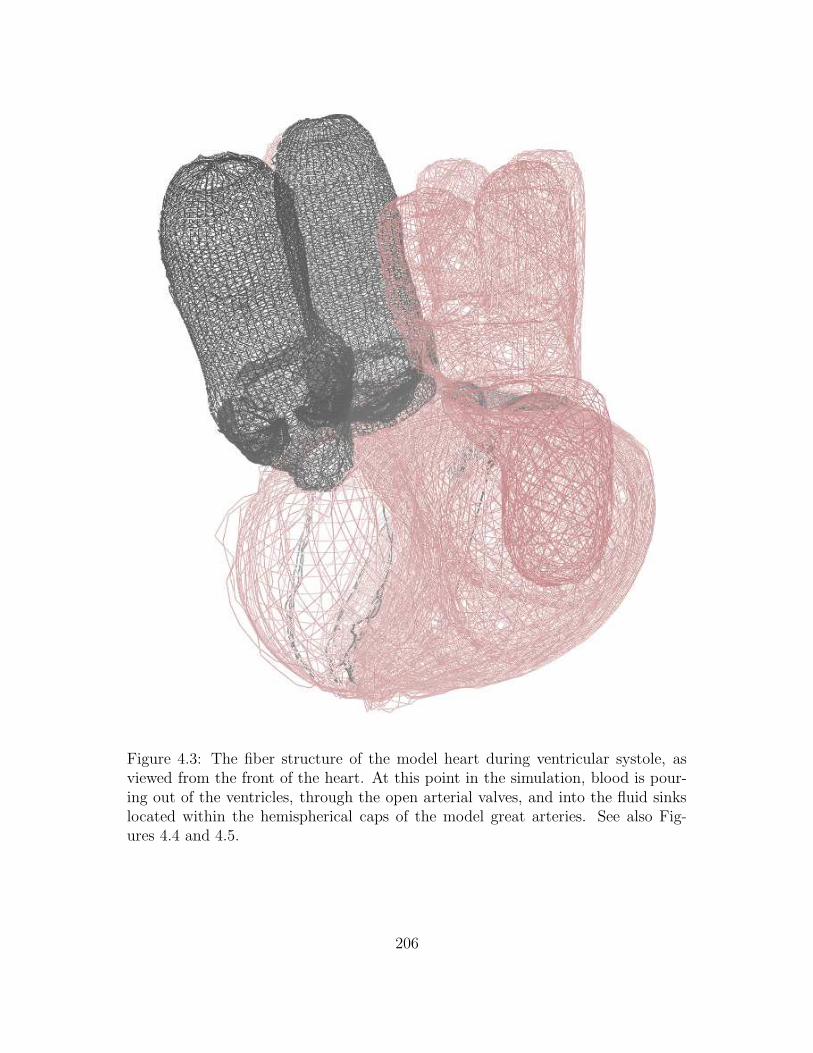
Figure 4.3: The fiber structure of the model heart during ventricular systole, asviewed from the front of the heart. At this point in the simulation, blood is pour-ing out of the ventricles, through the open arterial valves, and into the fluid sinkslocated within the hemispherical caps of the model great arteries. See also Fig-ures 4.4 and 4.5.

206

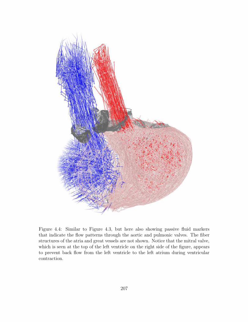
Figure 4.4: Similar to Figure 4.3, but here also showing passive fluid markersthat indicate the flow patterns through the aortic and pulmonic valves. The fiberstructures of the atria and great vessels are not shown. Notice that the mitral valve,which is seen at the top of the left ventricle on the right side of the figure, appearsto prevent back flow from the left ventricle to the left atrium during ventricularcontraction.

207

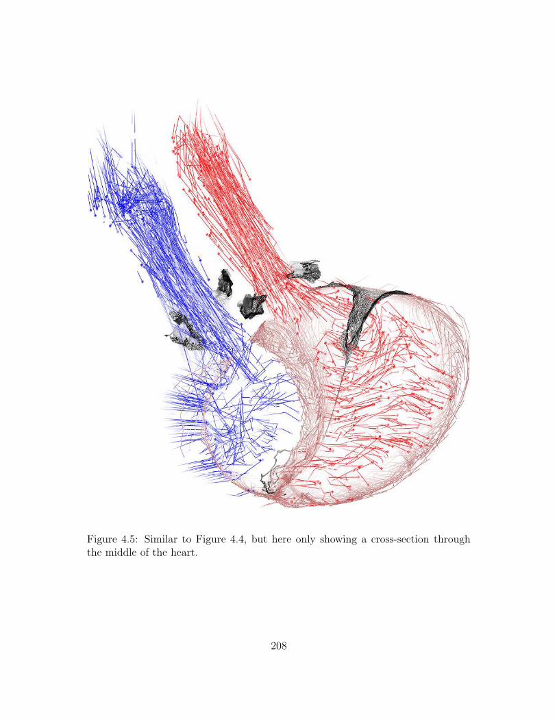
Figure 4.5: Similar to Figure 4.4, but here only showing a cross-section throughthe middle of the heart.

208

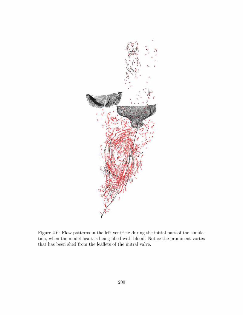
Figure 4.6: Flow patterns in the left ventricle during the initial part of the simula-tion, when the model heart is being filled with blood. Notice the prominent vortexthat has been shed from the leaflets of the mitral valve.

209

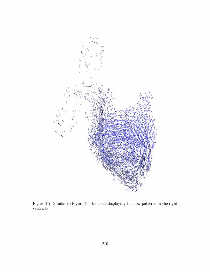
Figure 4.7: Similar to Figure 4.6, but here displaying the flow patterns in the rightventricle.

210

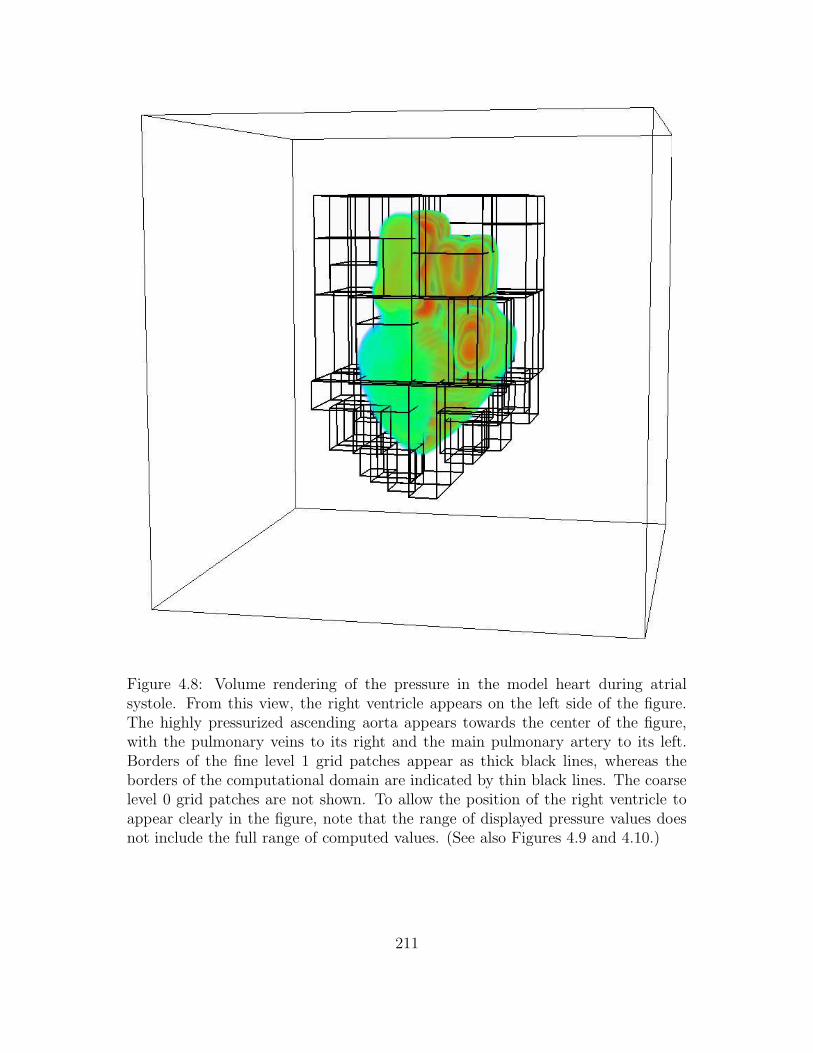
Figure 4.8: Volume rendering of the pressure in the model heart during atrialsystole. From this view, the right ventricle appears on the left side of the figure.The highly pressurized ascending aorta appears towards the center of the figure,with the pulmonary veins to its right and the main pulmonary artery to its left.Borders of the fine level 1 grid patches appear as thick black lines, whereas theborders of the computational domain are indicated by thin black lines. The coarselevel 0 grid patches are not shown. To allow the position of the right ventricle toappear clearly in the figure, note that the range of displayed pressure values doesnot include the full range of computed values. (See also Figures 4.9 and 4.10.)

211

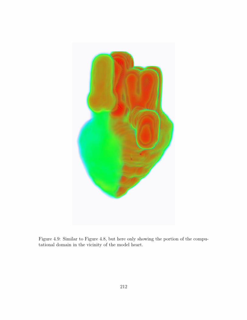
Figure 4.9: Similar to Figure 4.8, but here only showing the portion of the compu-tational domain in the vicinity of the model heart.

212

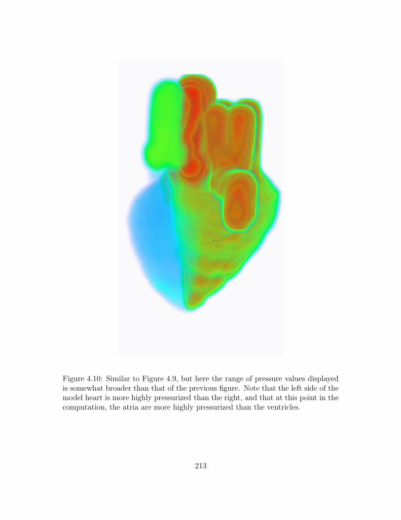
Figure 4.10: Similar to Figure 4.9, but here the range of pressure values displayedis somewhat broader than that of the previous figure. Note that the left side of themodel heart is more highly pressurized than the right, and that at this point in thecomputation, the atria are more highly pressurized than the ventricles.

213

4.4 Conclusions and directions for future work

In this chapter, we have demonstrated the successful application of the adaptive and

parallel methodology described in the present work to Peskin and McQueen’s three-

dimensional model of the heart and great vessels. It is important to emphasize,

however, that at the present time, we have made only limited use of the capabilities

provided by the adaptive version of the immersed boundary method. In particular,

although we believe that the present version of the immersed boundary method

yields somewhat more highly resolved results than previous versions at equivalent

spatial resolutions, the present adaptive computations do not employ finer spatial

grids than those used in the earlier work of Peskin and McQueen6. Instead, we

have used the adaptive methodology to “adaptively coarsen” the portions of the

computational domain that are exterior to the heart. Doing so does yield a modest

reduction in the computational demands of the model; however, making use of the

present adaptive methodology to obtain substantial increases in spatial resolution

remains future work. Although this is not a serious difficulty, note that performing

such simulations will require the construction of a more highly resolved fiber model

of the heart, as at higher Cartesian grid resolutions, the present fiber structure

would appear “porous.”

The full promise of adaptive methods for simulating cardiac mechanics perhaps

may not be realized until we are able to successfully deploy very high spatial res-

olution in a more localized fashion, e.g., only in the vicinity of the valves and the

vortices that have been shed from the free edges of the valve leaflets. The abil-

6In fact, to prevent failure of the arterial valves, the effective fine grid resolution employed inthe present simulation results is slightly coarser than that used in, e.g., [64, 52, 53].

214

ity to do so will require a generalization of the present adaptive scheme, since we

presently assume that the structures of the heart are embedded in the finest level

of the hierarchically composed Cartesian grid. The necessary generalizations are

fairly straightforward, and allowing portions of the heart (e.g., the muscular heart

walls) to be assigned to coarser levels of the locally refined grid should require only

minor modifications to the present computational framework. Nonetheless, this is

work that has not yet been done.

As we seek to obtain more highly resolved results, a more difficult challenge

will likely be posed by the stability constraint that limits the timestep size. In

the present version of the immersed boundary method, this constraint rapidly be-

comes quite severe as the spatial grid is refined. In particular, since we treat the

Lagrangian equations of motion in an explicit manner, the presence of bending-

resistant elements in the leaflets of the outflow valves results in a stability restric-

tion of the form ∆t = O(

h4`max

)

. Thus, until a computationally efficient implicit

version of the immersed boundary method is developed, it may not be feasible to

employ substantially finer grids than those used in the present work. Another,

possibly complementary avenue towards lessening the impact of such restrictions

on the timestep size is to develop a version of the adaptive method that employs

subcycling in time, whereby the timestep is refined locally along with the spatial

meshwidth. Such a method would at least allow for very small timesteps to be

employed only on a subset of the overall computational domain.

Recognizing these difficulties, we have attempted to design the implementation

of the present version of the immersed boundary method both so that it is useful as

a tool for performing large scale simulations, and so that it is useful as a platform

215

for developing future numerical methods. Although the degree to which we have

succeeded in meeting the first of these goals can be judged at least in part from the

simulation results of the present chapter, our success in developing a framework

that facilitates algorithmic development will only be demonstrated by future work.

Nonetheless, we believe that the present work represents a step towards the goal of

efficiently obtaining fully resolved simulations of cardiac mechanics.

216

Appendices

217

Appendix A

A three-dimensional fiber model

of the heart

The purpose of the present appendix is to summarize for the convenience of the

reader the major features of the three-dimensional fiber model of the heart and

great vessels developed by Peskin and McQueen [59, 63, 64, 52, 53]. A detailed

account of all of the technical details of this model is beyond the scope of the

present work, and the interested reader should consult the foregoing references for

a more complete description of the model. Instead, we focus here on describing the

features of the model that are most relevant to the simulation results presented in

Chapter 4.

The heart is a four chambered organ that consists of two pumps—the right and

left sides of the heart—that are responsible for pumping blood through the lungs

and through the peripheral organs, respectively. Each side of the heart consists

of two chambers, an atrium and a ventricle, with the weaker atrium acting as a

218

receiving chamber and as a primer pump for the more powerful ventricle. In the

body, the pulmonary veins supply oxygen-enriched blood from the lungs to the

left atrium, which in turn empties into the left ventricle through the mitral valve.

The muscular left ventricle ejects blood through the aortic valve into the ascending

aorta, through which it is distributed to all the tissues of the body (including the

heart itself via the coronary arteries). The corresponding structures of the right

side of the heart perform similar functions, but in this case the purpose of the heart

is to return oxygen-depleted blood to the lungs to be reoxygenated. In particular,

the superior and inferior vena cavae return blood from the tissues of the body to the

right atrium, which in turn empties into the right ventricle through the tricuspid

valve. The thin-walled right ventricle ejects blood through the pulmonic valve into

the pulmonary artery, through which the blood is returned to the lungs.

The two ventricles of the heart together form a structure that is often described

as possessing a somewhat conical shape, with an apex at the bottom of the heart

and a base towards the top. Although the axis of this cone is not constant as it

passes from apex to base, it is convenient (and traditional) to consider this axis

as being vertical in anatomical discussions of the isolated heart. (Note that from

this brief description of the shape of the ventricles, one might conclude that the

ventricles achieve their maximum diameter at the base of the heart. This is not

the case; rather, they are widest on a plane slightly below the base that is known

as the equatorial plane of the heart.) The valves of the heart are nearly coplanar

and essentially lie in the plane of the base. Above the base lie the ascending aorta

and the main pulmonary artery as well as the left and right atria, into which are

inserted the pulmonary veins and the superior and inferior vena cavae.

219

The three-dimensional model of the heart includes representations of each of

the major structural features of the heart and nearby great vessels. These include

the four chambers of the heart, i.e., the left and right ventricles and atria; the two

atrioventricular (inflow) valves; the two arterial (outflow) valves; the veins that

return blood to the atria, i.e., the pulmonary veins and the superior and inferior

vena cavae; and finally the major arteries that carry the blood ejected by the

ventricles, i.e., the ascending aorta and the main pulmonary artery. Each of these

structures is modeled as a system of elastic fibers: in the case of the valves, the fibers

mainly correspond to passive collagen fibers; in the great vessels, they correspond

to smooth muscle tissue; and in the myocardium, they correspond to active muscle

fibers that possess time-dependent contractile properties. Note that the model does

not include a detailed description of the circulation. Instead, the inflow and outflow

vessels all have blind ends, and fluid sources and sinks are provided to establish

realistic pressure loads on each side of the heart. (See also Section 4.2.2.)

The muscle fiber geometry of the model ventricles is based on the dissections of

C. E. Thomas, who chemically removed the connective tissue between the muscle

fascicles of porcine and canine hearts and then carefully tracked the spatial paths

of small bundles of fibers isolated with tweezers [73]. Thomas describes the ven-

tricular muscle fibers as being organized into a number of layers, with each fiber

beginning and ending at one of the valve rings. Each layer is described by Thomas

as consisting of two sheets: one on which fibers spiral away from the base, and

another on which they return to the base. The model of the ventricles includes a

subset of the layers qualitatively described by Thomas, namely:

220

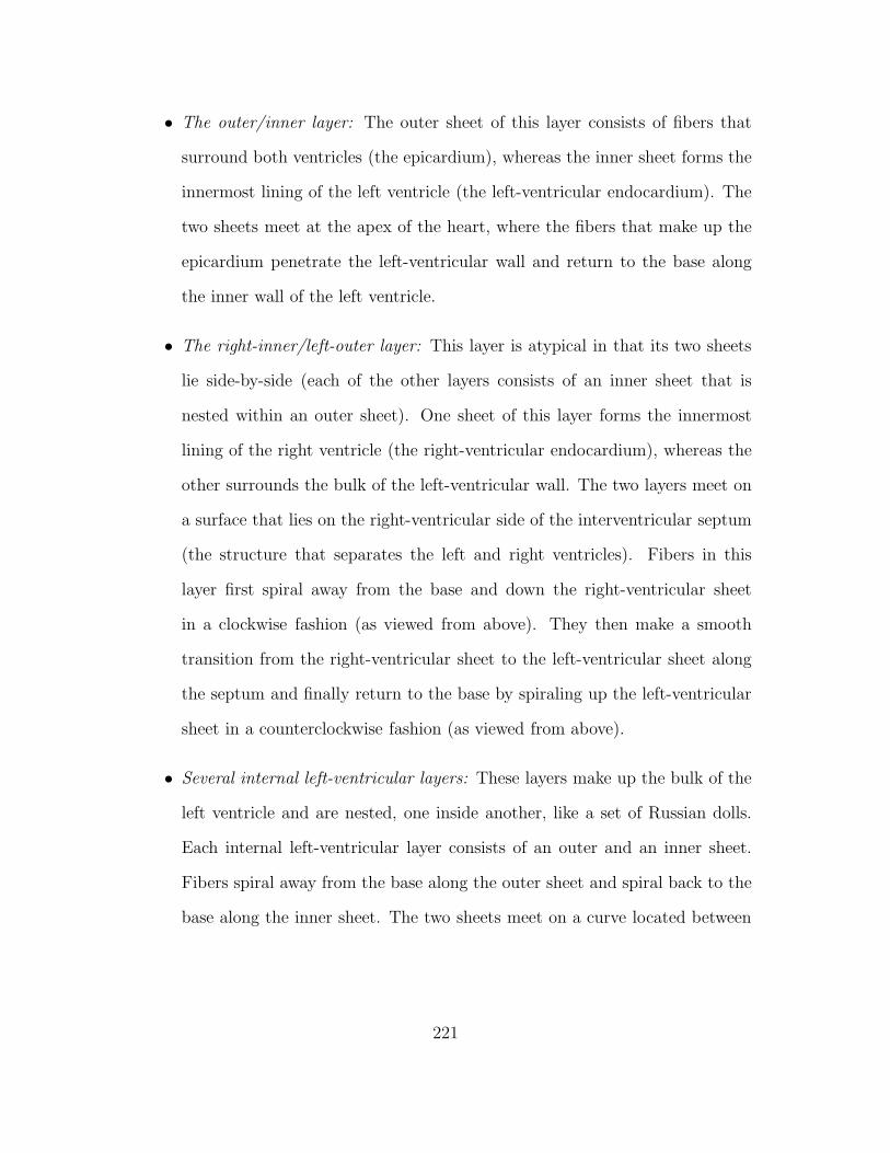
• The outer/inner layer: The outer sheet of this layer consists of fibers that

surround both ventricles (the epicardium), whereas the inner sheet forms the

innermost lining of the left ventricle (the left-ventricular endocardium). The

two sheets meet at the apex of the heart, where the fibers that make up the

epicardium penetrate the left-ventricular wall and return to the base along

the inner wall of the left ventricle.

• The right-inner/left-outer layer: This layer is atypical in that its two sheets

lie side-by-side (each of the other layers consists of an inner sheet that is

nested within an outer sheet). One sheet of this layer forms the innermost

lining of the right ventricle (the right-ventricular endocardium), whereas the

other surrounds the bulk of the left-ventricular wall. The two layers meet on

a surface that lies on the right-ventricular side of the interventricular septum

(the structure that separates the left and right ventricles). Fibers in this

layer first spiral away from the base and down the right-ventricular sheet

in a clockwise fashion (as viewed from above). They then make a smooth

transition from the right-ventricular sheet to the left-ventricular sheet along

the septum and finally return to the base by spiraling up the left-ventricular

sheet in a counterclockwise fashion (as viewed from above).

• Several internal left-ventricular layers: These layers make up the bulk of the

left ventricle and are nested, one inside another, like a set of Russian dolls.

Each internal left-ventricular layer consists of an outer and an inner sheet.

Fibers spiral away from the base along the outer sheet and spiral back to the

base along the inner sheet. The two sheets meet on a curve located between

221

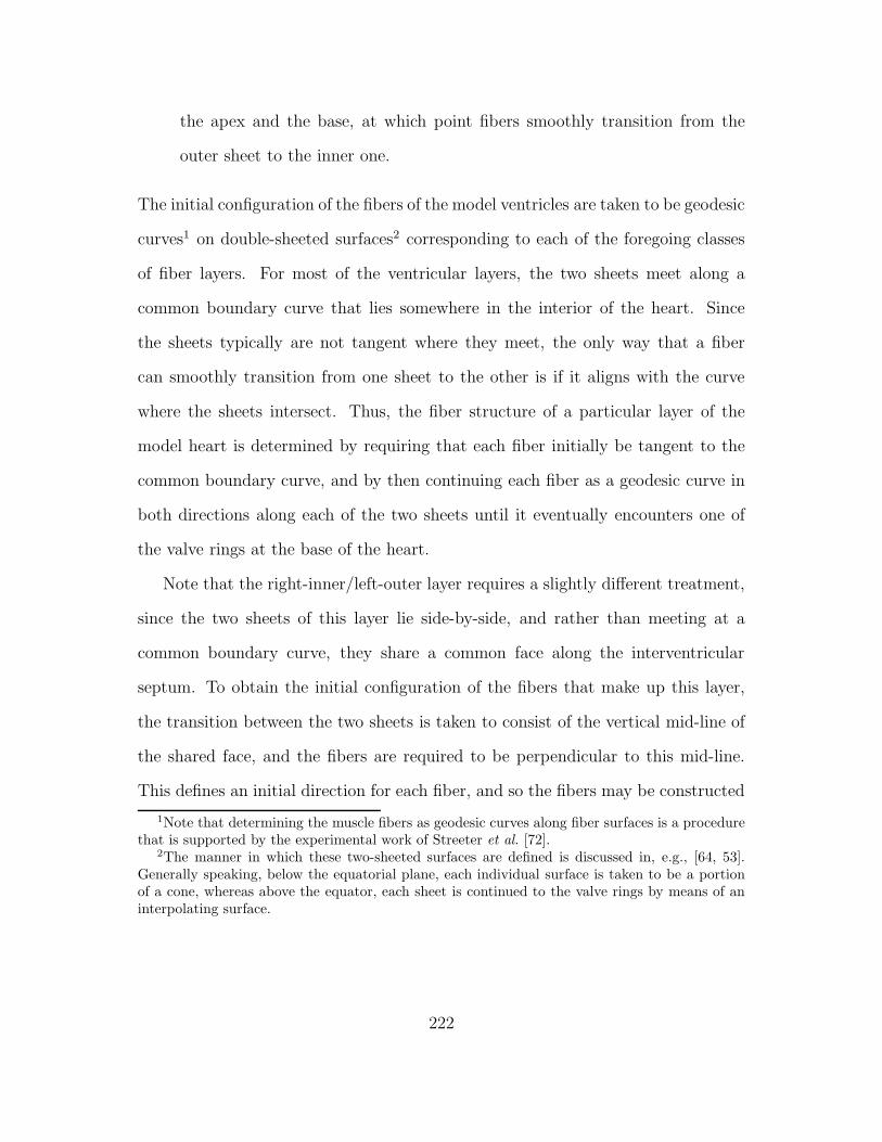
the apex and the base, at which point fibers smoothly transition from the

outer sheet to the inner one.

The initial configuration of the fibers of the model ventricles are taken to be geodesic

curves1 on double-sheeted surfaces2 corresponding to each of the foregoing classes

of fiber layers. For most of the ventricular layers, the two sheets meet along a

common boundary curve that lies somewhere in the interior of the heart. Since

the sheets typically are not tangent where they meet, the only way that a fiber

can smoothly transition from one sheet to the other is if it aligns with the curve

where the sheets intersect. Thus, the fiber structure of a particular layer of the

model heart is determined by requiring that each fiber initially be tangent to the

common boundary curve, and by then continuing each fiber as a geodesic curve in

both directions along each of the two sheets until it eventually encounters one of

the valve rings at the base of the heart.

Note that the right-inner/left-outer layer requires a slightly different treatment,

since the two sheets of this layer lie side-by-side, and rather than meeting at a

common boundary curve, they share a common face along the interventricular

septum. To obtain the initial configuration of the fibers that make up this layer,

the transition between the two sheets is taken to consist of the vertical mid-line of

the shared face, and the fibers are required to be perpendicular to this mid-line.

This defines an initial direction for each fiber, and so the fibers may be constructed

1Note that determining the muscle fibers as geodesic curves along fiber surfaces is a procedurethat is supported by the experimental work of Streeter et al. [72].

2The manner in which these two-sheeted surfaces are defined is discussed in, e.g., [64, 53].Generally speaking, below the equatorial plane, each individual surface is taken to be a portionof a cone, whereas above the equator, each sheet is continued to the valve rings by means of aninterpolating surface.

222

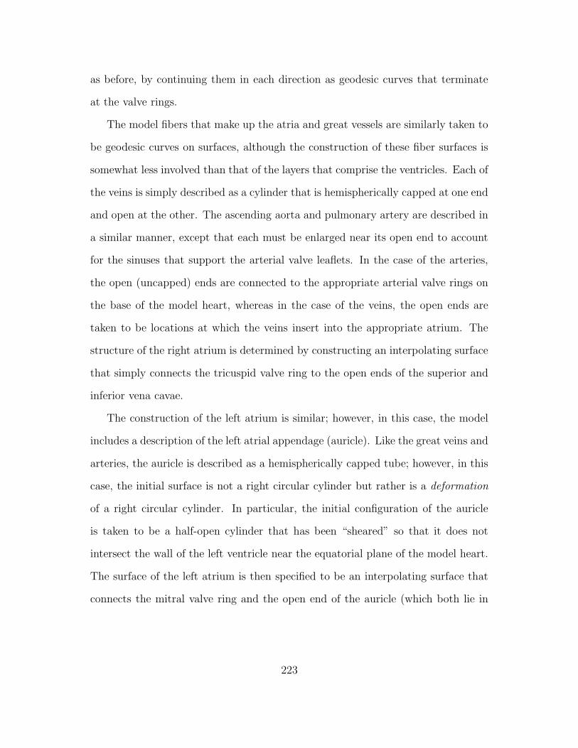
as before, by continuing them in each direction as geodesic curves that terminate

at the valve rings.

The model fibers that make up the atria and great vessels are similarly taken to

be geodesic curves on surfaces, although the construction of these fiber surfaces is

somewhat less involved than that of the layers that comprise the ventricles. Each of

the veins is simply described as a cylinder that is hemispherically capped at one end

and open at the other. The ascending aorta and pulmonary artery are described in

a similar manner, except that each must be enlarged near its open end to account

for the sinuses that support the arterial valve leaflets. In the case of the arteries,

the open (uncapped) ends are connected to the appropriate arterial valve rings on

the base of the model heart, whereas in the case of the veins, the open ends are

taken to be locations at which the veins insert into the appropriate atrium. The

structure of the right atrium is determined by constructing an interpolating surface

that simply connects the tricuspid valve ring to the open ends of the superior and

inferior vena cavae.

The construction of the left atrium is similar; however, in this case, the model

includes a description of the left atrial appendage (auricle). Like the great veins and

arteries, the auricle is described as a hemispherically capped tube; however, in this

case, the initial surface is not a right circular cylinder but rather is a deformation

of a right circular cylinder. In particular, the initial configuration of the auricle

is taken to be a half-open cylinder that has been “sheared” so that it does not

intersect the wall of the left ventricle near the equatorial plane of the model heart.

The surface of the left atrium is then specified to be an interpolating surface that

connects the mitral valve ring and the open end of the auricle (which both lie in

223

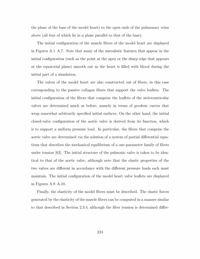
the plane of the base of the model heart) to the open ends of the pulmonary veins

above (all four of which lie in a plane parallel to that of the base).

The initial configuration of the muscle fibers of the model heart are displayed

in Figures A.1–A.7. Note that many of the unrealistic features that appear in the

initial configuration (such as the point at the apex or the sharp edge that appears

at the equatorial plane) smooth out as the heart is filled with blood during the

initial part of a simulation.

The valves of the model heart are also constructed out of fibers, in this case

corresponding to the passive collagen fibers that support the valve leaflets. The

initial configuration of the fibers that comprise the leaflets of the atrioventricular

valves are determined much as before, namely in terms of geodesic curves that

wrap somewhat arbitrarily specified initial surfaces. On the other hand, the initial

closed-valve configuration of the aortic valve is derived from its function, which

is to support a uniform pressure load. In particular, the fibers that comprise the

aortic valve are determined via the solution of a system of partial differential equa-

tions that describes the mechanical equilibrium of a one-parameter family of fibers

under tension [63]. The initial structure of the pulmonic valve is taken to be iden-

tical to that of the aortic valve, although note that the elastic properties of the

two valves are different in accordance with the different pressure loads each must

maintain. The initial configuration of the model heart valve leaflets are displayed

in Figures A.8–A.10.

Finally, the elasticity of the model fibers must be described. The elastic forces

generated by the elasticity of the muscle fibers can be computed in a manner similar

to that described in Section 2.3.4, although the fiber tension is determined differ-

224

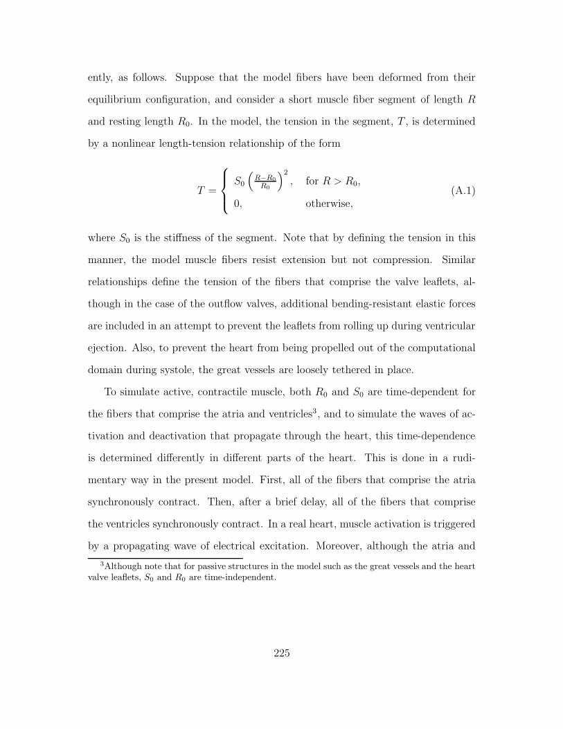
ently, as follows. Suppose that the model fibers have been deformed from their

equilibrium configuration, and consider a short muscle fiber segment of length R

and resting length R0. In the model, the tension in the segment, T , is determined

by a nonlinear length-tension relationship of the form

T =

S0

(

R−R0

R0

)2

, for R > R0,

0, otherwise,(A.1)

where S0 is the stiffness of the segment. Note that by defining the tension in this

manner, the model muscle fibers resist extension but not compression. Similar

relationships define the tension of the fibers that comprise the valve leaflets, al-

though in the case of the outflow valves, additional bending-resistant elastic forces

are included in an attempt to prevent the leaflets from rolling up during ventricular

ejection. Also, to prevent the heart from being propelled out of the computational

domain during systole, the great vessels are loosely tethered in place.

To simulate active, contractile muscle, both R0 and S0 are time-dependent for

the fibers that comprise the atria and ventricles3, and to simulate the waves of ac-

tivation and deactivation that propagate through the heart, this time-dependence

is determined differently in different parts of the heart. This is done in a rudi-

mentary way in the present model. First, all of the fibers that comprise the atria

synchronously contract. Then, after a brief delay, all of the fibers that comprise

the ventricles synchronously contract. In a real heart, muscle activation is triggered

by a propagating wave of electrical excitation. Moreover, although the atria and

3Although note that for passive structures in the model such as the great vessels and the heartvalve leaflets, S0 and R0 are time-independent.

225

ventricles contract in a coordinated manner in a healthy heart, they do not do so

synchronously. The inclusion of more realistic muscle activation patterns into this

model of cardiac mechanics, possibly by means of a realistic electrophysiological

model, remains important future work.

226

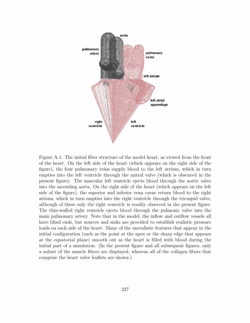
Figure A.1: The initial fiber structure of the model heart, as viewed from the frontof the heart. On the left side of the heart (which appears on the right side of thefigure), the four pulmonary veins supply blood to the left atrium, which in turnempties into the left ventricle through the mitral valve (which is obscured in thepresent figure). The muscular left ventricle ejects blood through the aortic valveinto the ascending aorta. On the right side of the heart (which appears on the leftside of the figure), the superior and inferior vena cavae return blood to the rightatrium, which in turn empties into the right ventricle through the tricuspid valve,although of these only the right ventricle is readily observed in the present figure.The thin-walled right ventricle ejects blood through the pulmonic valve into themain pulmonary artery. Note that in the model, the inflow and outflow vessels allhave blind ends, but sources and sinks are provided to establish realistic pressureloads on each side of the heart. Many of the unrealistic features that appear in theinitial configuration (such as the point at the apex or the sharp edge that appearsat the equatorial plane) smooth out as the heart is filled with blood during theinitial part of a simulation. (In the present figure and all subsequent figures, onlya subset of the muscle fibers are displayed, whereas all of the collagen fibers thatcomprise the heart valve leaflets are shown.)

227

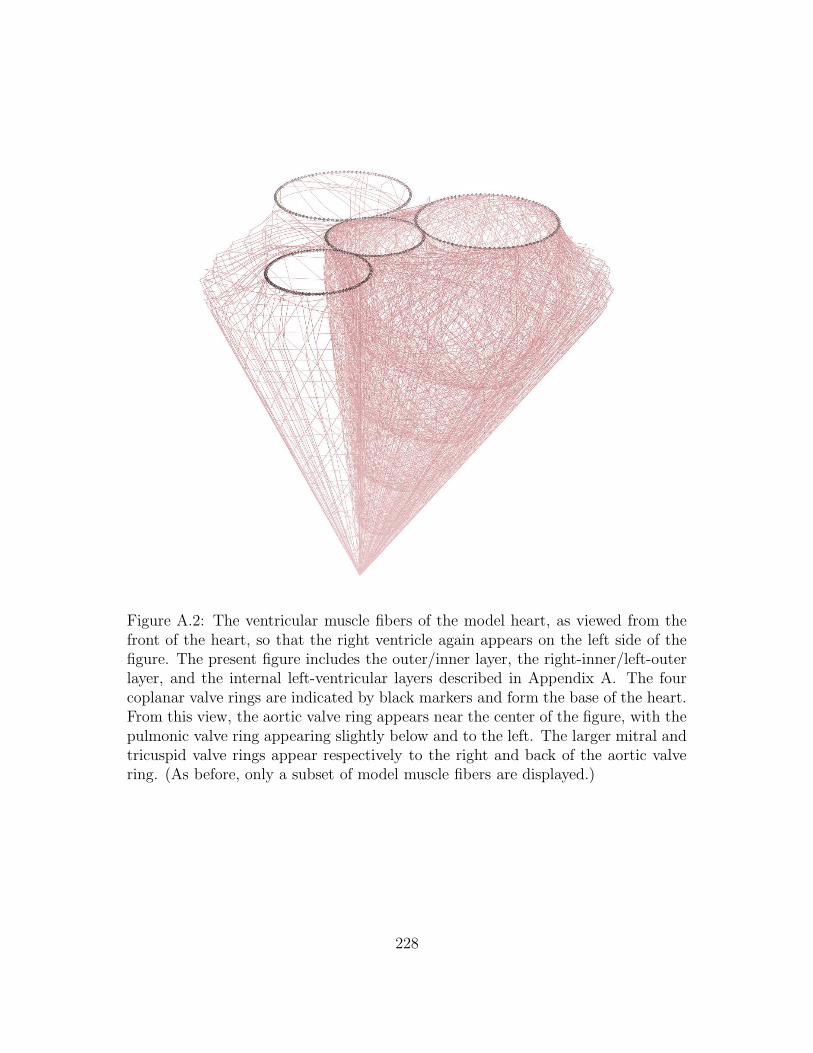
Figure A.2: The ventricular muscle fibers of the model heart, as viewed from thefront of the heart, so that the right ventricle again appears on the left side of thefigure. The present figure includes the outer/inner layer, the right-inner/left-outerlayer, and the internal left-ventricular layers described in Appendix A. The fourcoplanar valve rings are indicated by black markers and form the base of the heart.From this view, the aortic valve ring appears near the center of the figure, with thepulmonic valve ring appearing slightly below and to the left. The larger mitral andtricuspid valve rings appear respectively to the right and back of the aortic valvering. (As before, only a subset of model muscle fibers are displayed.)

228

Figure A.3: The four nested internal left-ventricular layers of the model heartdescribed in Appendix A, as viewed from the front of the heart. The valve ringsare again indicated by black markers. The larger mitral valve ring is the location atwhich the left atrium joins the left ventricle, whereas the smaller aortic valve ringis the location at which the ascending aorta is attached. (As before, only a subsetof model muscle fibers are displayed.)

229

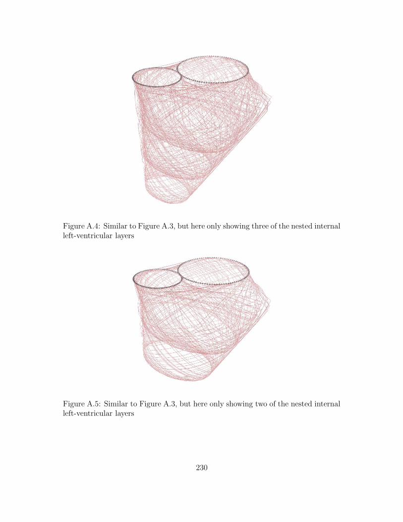
Figure A.4: Similar to Figure A.3, but here only showing three of the nested internalleft-ventricular layers

Figure A.5: Similar to Figure A.3, but here only showing two of the nested internalleft-ventricular layers

230

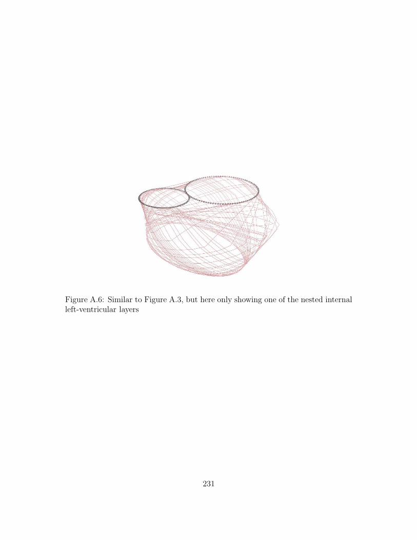
Figure A.6: Similar to Figure A.3, but here only showing one of the nested internalleft-ventricular layers

231

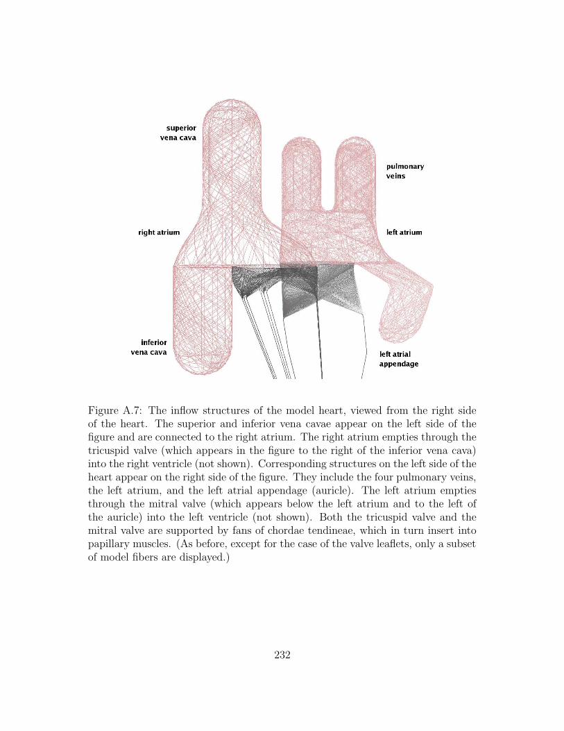
Figure A.7: The inflow structures of the model heart, viewed from the right sideof the heart. The superior and inferior vena cavae appear on the left side of thefigure and are connected to the right atrium. The right atrium empties through thetricuspid valve (which appears in the figure to the right of the inferior vena cava)into the right ventricle (not shown). Corresponding structures on the left side of theheart appear on the right side of the figure. They include the four pulmonary veins,the left atrium, and the left atrial appendage (auricle). The left atrium emptiesthrough the mitral valve (which appears below the left atrium and to the left ofthe auricle) into the left ventricle (not shown). Both the tricuspid valve and themitral valve are supported by fans of chordae tendineae, which in turn insert intopapillary muscles. (As before, except for the case of the valve leaflets, only a subsetof model fibers are displayed.)

232

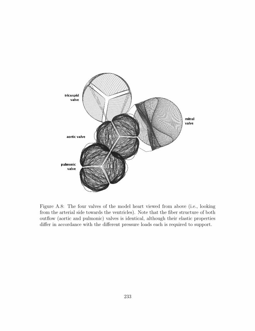
Figure A.8: The four valves of the model heart viewed from above (i.e., lookingfrom the arterial side towards the ventricles). Note that the fiber structure of bothoutflow (aortic and pulmonic) valves is identical, although their elastic propertiesdiffer in accordance with the different pressure loads each is required to support.

233

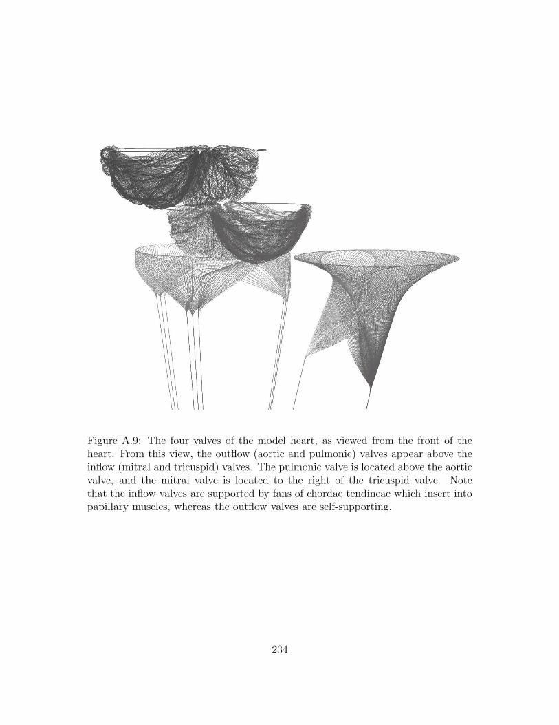
Figure A.9: The four valves of the model heart, as viewed from the front of theheart. From this view, the outflow (aortic and pulmonic) valves appear above theinflow (mitral and tricuspid) valves. The pulmonic valve is located above the aorticvalve, and the mitral valve is located to the right of the tricuspid valve. Notethat the inflow valves are supported by fans of chordae tendineae which insert intopapillary muscles, whereas the outflow valves are self-supporting.

234

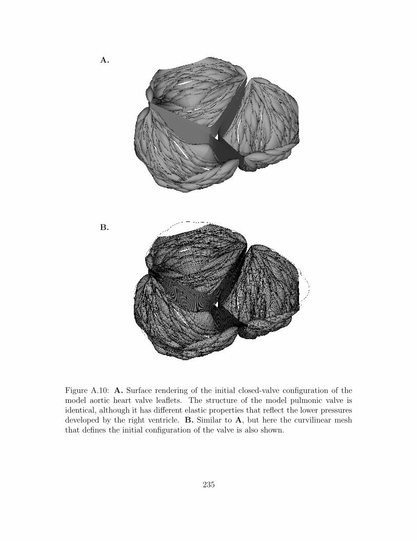
A.

B.

Figure A.10: A. Surface rendering of the initial closed-valve configuration of themodel aortic heart valve leaflets. The structure of the model pulmonic valve isidentical, although it has different elastic properties that reflect the lower pressuresdeveloped by the right ventricle. B. Similar to A, but here the curvilinear meshthat defines the initial configuration of the valve is also shown.

235

Appendix B

Incompressible fluid dynamics

with distributed sources and sinks

This appendix provides for the convenience of the reader a slightly edited tran-

scription of a set of unpublished notes by C. S. Peskin on the formulation of the

equations of motion for a viscous incompressible fluid in the case that there are

fluid sources or sinks distributed within the domain occupied by the fluid [60].

Note that in the present appendix, it is convenient to denote the components

of the (Eulerian) velocity by u = (u1, u2, u3). Also note that δij is taken to be the

familiar Kronecker delta function, i.e.,

δij =

1, if i = j,

0, otherwise.(B.1)

236

B.1 The modified equations of motion

We consider a viscous incompressible fluid with uniform density, ρ, and uniform

dynamic viscosity, µ. The fluid fills all of three-dimensional space (or, alternatively,

it fills a periodic box U ⊂ IR3). In either case, let U be the domain occupied by the

fluid. To accommodate fluid sources and sinks that are distributed within U , we

assume that the fluid is locally created or destroyed at net rate qsrc(x, t), so that

∇ · u(x, t) = qsrc(x, t). (B.2)

In the periodic case, we require that qsrc satisfy the compatibility condition

∫

U

qsrc(x, t) dx = 0. (B.3)

Otherwise, if U = IR3, qsrc(x, t) is arbitrary.

Our purpose is to define the equations of motion for such a fluid. Doing so

requires that we make several additional assumptions regarding its properties. Our

choices are as follows:

(i) The creation of fluid does not introduce any additional momentum. That is,

at a fluid source, fluid is created with zero momentum and then immediately

suffers an inelastic collision with the existing fluid in the neighborhood of the

source. This collision brings the newly created fluid up to the local velocity,

u(x, t), at the price of converting some kinetic energy into heat (in an amount

that is calculated below in Section B.2).

237

(ii) When a parcel of fluid is destroyed at a fluid sink, its momentum is destroyed

also.

(iii) The stress tensor of the fluid is, as usual,

σij = −p δij + µ

(

∂ui

∂xj

+∂uj

∂xi

− 2

3qsrcδij

)

, (B.4)

recalling that ∇ · u(x, t) = qsrc(x, t).

As we shall see, Assumptions (i) and (ii) are asymmetric with respect to the creation

(qsrc(x, t) > 0) and destruction (qsrc(x, t) < 0) of fluid. Anticipating this, we define

q+src(x, t) =

qsrc(x, t), if qsrc(x, t) ≥ 0,

0, if qsrc(x, t) ≤ 0,(B.5)

q−src(x, t) =

0, if qsrc(x, t) ≥ 0,

qsrc(x, t), if qsrc(x, t) ≤ 0.(B.6)

Thus, q+src ≥ 0, q−src ≤ 0, qsrc = q+

src + q−src, and |qsrc| = q+src − q−src.

Now, consider a fixed region of space V ⊂ U with surface ∂V and outward unit

normal n. Let Pi(V, t) be the ith component of the momentum within the region

V , for i = 1, 2, 3. Then

Pi(V, t) =

∫

V

ρui dx, (B.7)

and

dPi

dt(V, t) =

∫

V

ρ∂ui

∂tdx. (B.8)

238

According to our assumptions, however, we also have that

dPi

dt(V, t) =

∫

∂V

3∑

j=1

(

−p δij + µ

(

∂ui

∂xj+∂uj

∂xi− 2

3qsrcδij

))

nj dS (B.9)

−∫

∂V

ρui

3∑

j=1

(njuj) dS +

∫

V

ρuiq−src dx.

(Recall that q−src ≤ 0.) The last term in (B.9) is the only one that is non-standard.

It accounts for the destruction of momentum, along with the fluid in which that mo-

mentum used to reside, at fluid sinks (see Assumption (ii)). According to Assump-

tion (i), however, there is no corresponding term at fluid sources, where qsrc > 0.

This is the asymmetry mentioned above.

Combining equations (B.8) and (B.9) and applying the divergence theorem, we

find that

∫

V

ρ∂ui

∂t− ρuiq

−src +

3∑

j=1

∂

∂xj

((

p+2

3µqsrc

)

δij + ρuiuj (B.10)

− µ(

∂ui

∂xj

+∂uj

∂xi

))

dx = 0.

Since the choice of V ⊂ U is arbitrary, the integrand must be zero. Therefore,

making use of equation (B.2), we obtain

ρ

(

∂ui

∂t+

3∑

j=1

∂

∂xj

(uiuj)

)

+∂

∂xi

(

p− 1

3µqsrc

)

= µ3∑

j=1

∂2ui

∂x2j

+ ρuiq−src. (B.11)

Note that the term p+ 23µqsrc in equation (B.10) has become p− 1

3µqsrc in equation

239

(B.11). The additional −µqsrc comes from the identity

3∑

j=1

∂

∂xj

∂uj

∂xi=∂qsrc∂xi

. (B.12)

Equation (B.11) resembles the standard Navier-Stokes equation for a viscous in-

compressible fluid written in conservation form, but note that there are two new

features. One is that p− 13µqsrc plays the role of the pressure. The other is the term

ρuiq−src, which introduces a kind of friction since q−src ≤ 0.

Two alternate forms of (B.11) are also of interest. They are obtained by ma-

nipulating the nonlinear terms. First, note the identities

3∑

j=1

∂

∂xj

(uiuj) =3∑

j=1

∂ui

∂xj

uj + ui

3∑

j=1

∂uj

∂xj

=3∑

j=1

∂ui

∂xj

uj + uiqsrc, (B.13)

and

q−src − qsrc = −q+src, (B.14)

q−src −1

2qsrc =

1

2

(

q−src − q+src

)

= −1

2|qsrc|. (B.15)

These identities allow us to rewrite equation (B.11) in either of the two equivalent

forms:

ρ

(

∂ui

∂t+

3∑

j=1

∂ui

∂xjuj

)

+∂

∂xi

(

p− 1

3µqsrc

)

= µ

3∑

j=1

∂2ui

∂x2j

− ρuiq+src, (B.16)

240

and

ρ

(

∂ui

∂t+

1

2

3∑

j=1

∂

∂xj(uiuj) +

1

2

3∑

j=1

∂ui

∂xjuj

)

+∂

∂xi

(

p− 1

3µqsrc

)

= (B.17)

= µ3∑

j=1

∂2ui

∂x2j

− 1

2ρui|qsrc|.

(In the present work, we make use of equation (B.16) in developing numerical

methods for the modified equations of motion, whereas equation (B.17) is employed

below to determine the rate of kinetic energy dissipation at the sources and sinks.)

B.2 The rate of dissipation of kinetic energy as-

sociated with fluid sources and sinks

Next, we consider the dissipation of kinetic energy associated with the sources and

sinks. For this purpose, the most convenient of the three equivalent forms of the

equations of motion is the last one, equation (B.17). To proceed, multiply both

sides of equation (B.17) by ui, sum over i, and integrate over the domain occupied

by the fluid, U . Integration by parts shows that the nonlinear term in equation

(B.17) makes no contribution to the rate of dissipation (which is why this form of

the equations is convenient for the present purpose), and we are left with

d

dt

∫

U

1

2ρ‖u‖2 dx =

∫

U

pqsrc−1

3µq2

src−µ3∑

i=1

3∑

j=1

(

∂ui

∂xj

)2

− 1

2ρ‖u‖2|qsrc| dx. (B.18)

241

The viscous terms may be put in a more standard form in the following way. Let

Dij =∂ui

∂xj+∂uj

∂xi− 2

3qsrcδij, (B.19)

where, as before, ∇ · u = qsrc. Then,

∫

U

3∑

i=1

3∑

j=1

Dij∂ui

∂xjdx =

∫

U

3∑

i=1

3∑

j=1

(

(

∂ui

∂xj

)2

+∂ui

∂xj

∂uj

∂xi

)

− 2

3q2src dx, (B.20)

but, integrating by parts twice to switch the derivatives yields

∫

U

3∑

i=1

3∑

j=1

∂ui

∂xj

∂uj

∂xidx =

∫

U

3∑

i=1

3∑

j=1

∂ui

∂xi

∂uj

∂xjdx =

∫

U

q2src dx. (B.21)

Therefore,

∫

U

3∑

i=1

3∑

j=1

Dij∂ui

∂xj

dx =

∫

U

3∑

i=1

3∑

j=1

(

∂ui

∂xj

)2

+1

3q2src dx. (B.22)

Substituting equation (B.22) into the energy balance equation, equation (B.18), we

obtain

d

dt

∫

U

1

2ρ‖u‖2 dx =

∫

U

pqsrc − µ3∑

i=1

3∑

j=1

Dij∂ui

∂xj− 1

2ρ‖u‖2|qsrc| dx. (B.23)

The interpretation of equation (B.23) is as follows: The left-hand side is the

rate of change of kinetic energy. On the right-hand side, the first term,

∫

U

pqsrc dx, (B.24)

242

is the net rate at which work is done by the sources and sinks against the pressure

field of the fluid.

The next term,

+µ

∫

U

3∑

i=1

3∑

j=1

Dij∂ui

∂xj

dx, (B.25)

(which appears in equation (B.23) with a minus sign) is the rate of viscous energy

dissipation into heat. Note that it is possible to rewrite this term in the form

+µ

2

∫

U

3∑

i=1

3∑

j=1

D2ij dx, (B.26)

although we skip the details of deriving this.

Finally, the term

+

∫

U

1

2ρ‖u‖2|q| dx (B.27)

(which also appears in equation (B.23) with a minus sign) is the rate of kinetic

energy dissipation by the sources and sinks.

In the case of a fluid sink, the origin of this last term is clear, since by Assump-

tion (ii), the destruction of a fluid element involves the destruction of its momentum

and hence also its kinetic energy.

In the case of a fluid source, the interpretation is more subtle. By Assumption

(i), when a fluid element is created at a source, it possesses no momentum and

hence no kinetic energy. Newly created fluid elements acquire momentum and

kinetic energy through an inelastic collision with the surrounding fluid. To analyze

such a collision, consider a particle of mass M and velocity W that collides with

a particle of mass m that is initially at rest. In the case of an extreme inelastic

243

collision, following the collision the particles stick together. Their common velocity,

W ′, is determined by conservation of momentum,

MW = (M +m)W ′, (B.28)

and the kinetic energies before and after the collision are respectively given by

E =1

2MW 2, (B.29)

E ′ =1

2(M +m)(W ′)2 =

1

2(M +m)

(

M

M +m

)2

W 2. (B.30)

Thus, the change in kinetic energy is

∆E = E ′ − E =1

2MW 2

(

M

M +m− 1

)

(B.31)

= −1

2

Mm

M +mW 2.

In the case that m M , MmM+m

≈ m, and thus in this case an amount of kinetic

energy approximately equal to 12mW 2 is converted into heat by the extreme inelastic

collision. This result is essentially the same as the last term in equation (B.23) at

a fluid source.

244

B.3 Summary of the equations of motion

In summary, the equations of motion are

∇ · u = qsrc, (B.32)

together with any of the following three equivalent forms:

ρ

(

∂ui

∂t+

3∑

j=1

∂

∂xj(uiuj)

)

+∂

∂xi

(

p− 1

3µqsrc

)

= µ

3∑

j=1

∂2ui

∂x2j

+ ρuiq−src, (B.33)

ρ

(

∂ui

∂t+

3∑

j=1

∂ui

∂xjuj

)

+∂

∂xi

(

p− 1

3µqsrc

)

= µ

3∑

j=1

∂2ui

∂x2j

− ρuiq+src, (B.34)

or

ρ

(

∂ui

∂t+

1

2

3∑

j=1

∂

∂xj

(uiuj) +1

2

3∑

j=1

∂ui

∂xj

uj

)

+∂

∂xi

(

p− 1

3µqsrc

)

= (B.35)

= µ

3∑

j=1

∂2ui

∂x2j

− 1

2ρui|qsrc|.

The main result of this Appendix is that the correct version of the “friction”

term associated with fluid sources and sinks depends on the manner in which the

nonlinear terms of the Navier-Stokes equations are written. In particular, when

these equations are written in the “conservative” form, (B.33), then friction appears

in the equations as though localized only at the sinks; when the nonlinear terms are

written in what may be called the “non-conservative” or “transport” form, (B.34),

then friction appears in the equations as though localized only at the sources;

245

and finally, when the nonlinear terms are written in the intermediate or “skew-

symmetric” form, (B.35), then friction appears in the equations as though acting

at sources and sinks alike.

246

Bibliography

[1] M. F. Adams, M. Brezina, J. J. Hu, and R. S. Tuminaro. Parallel multi-

grid smoothing: polynomial versus Gauss-Seidel. Journal of Computational

Physics, 188(2):593–610, 2003.

[2] A. S. Almgren, J. B. Bell, P. Colella, L. H. Howell, and M. L. Welcome. A

conservative adaptive projection method for the variable density incompress-

ible Navier-Stokes equations. Journal of Computational Physics, 142(1):1–46,

1998.

[3] A. S. Almgren, J. B. Bell, and W. Y. Crutchfield. Approximate projection

methods: Part I. Inviscid analysis. SIAM Journal on Scientific Computing,

22(4):1139–1159, 2000.

[4] A. S. Almgren, J. B. Bell, and W. G. Szymczak. A numerical method for the

incompressible Navier-Stokes equations based on an approximate projection.

SIAM Journal on Scientific Computing, 17(2):358–369, 1996.

[5] American Heart Association. Heart Disease and Stroke Statistics—2005 up-

date. American Heart Association, Dallas, TX, USA, 2004.

247

[6] S. F. Ashby and R. D. Falgout. A parallel multigrid preconditioned conjugate

gradient algorithm for groundwater flow simulations. Nuclear Science and

Engineering, 124(1):145–159, 1996. Also available as LLNL Technical Report

UCRL-JC-122359.

[7] S. Balay, K. Buschelman, V. Eijkhout, W. D. Gropp, D. Kaushik, M. G.

Knepley, L. C. McInnes, B. F. Smith, and H. Zhang. PETSc Users Manual.

Technical Report ANL-95/11 - Revision 2.1.5, Argonne National Laboratory,

2004.

[8] S. Balay, K. Buschelman, W. D. Gropp, D. Kaushik, M. G. Knep-

ley, L. C. McInnes, B. F. Smith, and H. Zhang. PETSc Web page.

http://www.mcs.anl.gov/petsc.

[9] S. Balay, V. Eijkhout, W. D. Gropp, L. C. McInnes, and B. F. Smith. Efficient

management of parallelism in object oriented numerical software libraries. In

E. Arge, A. M. Bruaset, and H. P. Langtangen, editors, Modern Software Tools

in Scientific Computing, pages 163–202. Birkhauser Press, 1997.

[10] R. Barrett, M. Berry, T. F. Chan, J. Demmel, J. Donato, J. Dongarra, V. Ei-

jkhout, R. Pozo, C. Romine, and H. Van der Vorst. Templates for the Solution

of Linear Systems: Building Blocks for Iterative Methods, Second Edition. So-

ciety for Industrial and Applied Mathematics, Philadelphia, PA, USA, 1994.

Also available from http://www.netlib.org/templates.

248

[11] J. B. Bell, P. Colella, and H. M. Glaz. A second-order projection method for

the incompressible Navier-Stokes equations. Journal of Computational Physics,

85(2):257–283, 1989.

[12] M. J. Berger and P. Colella. Local adaptive mesh refinement for shock hydro-

dynamics. Journal of Computational Physics, 82(1):64–84, 1989.

[13] M. J. Berger and J. Oliger. Adaptive mesh refinement for hyperbolic partial-

differential equations. Journal of Computational Physics, 53(3):484–512, 1984.

[14] M. J. Berger and I. Rigoutsos. An algorithm for point clustering and grid

generation. IEEE Transactions on Systems, Man and Cybernetics, 21(5):1278–

1286, 1991.

[15] W. L. Briggs, V. E. Henson, and S. F. McCormick. A Multigrid Tutorial,

Second Edition. Society for Industrial and Applied Mathematics, Philadelphia,

PA, USA, 2000.

[16] D. L. Brown, R. Cortez, and M. L. Minion. Accurate projection methods for

the incompressible Navier-Stokes equations. Journal of Computational Physics,

168(2):464–499, 2001.

[17] T. F. Chan and T. P. Mathew. Domain decomposition algorithms. Acta

Numerica, 3:61–143, 1994.

[18] A. J. Chorin. Numerical solution of the Navier-Stokes equations. Mathematics

of Computation, 22(104):745–762, 1968.

249

[19] A. J. Chorin. On the convergence of discrete approximations to the Navier-

Stokes equations. Mathematics of Computation, 23(106):341–353, 1969.

[20] P. Colella. Multidimensional upwind methods for hyperbolic conservation laws.

Journal of Computational Physics, 87(1):171–200, 1989.

[21] R. K. Crockett, P. Colella, R. T. Fisher, R. I. Klein, and C. F. McKee. An un-

split, cell-centered Godunov method for ideal MHD. Journal of Computational

Physics, 203(2):422–448, 2005.

[22] J. W. Demmel. Applied Numerical Linear Algebra. Society for Industrial and

Applied Mathematics, Philadelphia, PA, USA, 1997.

[23] T. Dombre, U. Frisch, J. M. Greene, M. Henon, A. Mehr, and A. M. Soward.

Chaotic streamlines in the ABC flows. Journal of Fluid Mechanics, 167:353–

391, 1986.

[24] R. E. Ewing, R. D. Lazarov, and P. S. Vassilevski. Local refinement techniques

for elliptic problems on cell-centered grids I. Error analysis. Mathematics of

Computation, 56(194):437–461, 1991.

[25] R. D. Falgout and J. E. Jones. Multigrid on massively parallel architectures.

In E. Dick, K. Riemslagh, and J. Vierendeels, editors, Multigred Methods VI,

volume 14 of Lecture Notes in Computational Science and Engineering, pages

101–107. Springer, 2000. Also available as LLNL Technical Report UCRL-JC-

133948.

250

[26] R. D. Falgout and U. M. Yang. hypre: a library of high performance pre-

conditioners. In P. M. A. Sloot, C. J. K. Tan, J. J. Dongarra, and A. G.

Hoekstra, editors, Computational Science - ICCS 2002 Part III, volume 2331

of Lecture Notes in Computer Science, pages 632–641. Springer–Verlag, 2002.

Also available as LLNL Technical Report UCRL-JC-146175.

[27] E. Gamma, R. Helm, R. Johnson, and J. Vlissides. Design Patterns: Elements

of Reusable Object-Oriented Software. Addison-Wesley, 1995.

[28] S. Gottlieb, C.-W. Shu, and E. Tadmor. Strong stability-preserving high-order

time discretization methods. SIAM Review, 43(1):89–112, 2001.

[29] B. E. Griffith and C. S. Peskin. On the order of accuracy of the immersed

boundary method: Higher order convergence rates for sufficiently smooth prob-

lems. Journal of Computational Physics, 208(1):75–105, 2005.

[30] W. Gropp, E. Lusk, and A. Skjellum. Using MPI: Portable Parallel Program-

ming with the Message-Passing Interface, Second Edition. The MIT Press,

Cambridge, MA, USA, 1999.

[31] A. C. Guyton and J. E. Hall. Textbook of Medical Physiology, Tenth Edition.

W. B. Saunders Company, Philadelphia, PA, USA, 2000.

[32] F. H. Harlow and J. E. Welch. Numerical calculation of time-dependent viscous

incompresible flow of fluid with free surface. Physics of Fluids, 8(12):2182–

2189, 1965.

251

[33] R. D. Hornung and S. R. Kohn. Managing application complexity in the

SAMRAI object-oriented framework. Concurrency and Computation: Practice

and Experience, 14(5):347–368, 2002.

[34] L. H. Howell and J. B. Bell. An adaptive mesh projection method for viscous

incompressible flow. SIAM Journal on Scientific Computing, 18(4):996–1013,

1997.

[35] hypre: High performance preconditioners. http://www.llnl.gov/CASC/hypre.

[36] M. F. Lai. A projection method for reacting flow in the zero mach number

limit. PhD thesis, University of California at Berkeley, 1993.

[37] B. Lee, S. F. McCormick, B. Philip, and D. J. Quinlan. Asynchronous fast

adaptive composite-grid methods for elliptic problems: Numerical results.

SIAM Journal on Scientific Computing, 25(2):682–700, 2003.

[38] B. Lee, S. F. McCormick, B. Philip, and D. J. Quinlan. Asynchronous fast

adaptive composite-grid methods for elliptic problems: Theoretical founda-

tions. SIAM Journal on Numerical Analysis, 42(1):130–152, 2004.

[39] L. Lee and R. J. Leveque. An immersed interface method for incompressible

Navier-Stokes equations. SIAM Journal on Scientific Computing, 25(3):832–

856, 2003.

[40] R. J. LeVeque. Finite Volume Methods for Hyperbolic Problems. Cambridge

University Press, 2002.

252

[41] R. J. Leveque and Z. Li. Immersed interface methods for Stokes flow with

elastic boundaries or surface tension. SIAM Journal on Scientific Computing,

18(3):709–735, 1997.

[42] D. F. Martin and P. Colella. A cell-centered adaptive projection method

for the incompressible Euler equations. Journal of Computational Physics,

163(2):271–312, 2000.

[43] A. A. Mayo and C. S. Peskin. An implicit numerical method for fluid dy-

namics problems with immersed elastic boundaries. In A. Y. Cheer and C. P.

van Dam, editors, Fluid Dynamics in Biology: Proceedings of an AMS-IMS-

SIAM Joint Summer Research Conference, volume 140 of Contemporary Math-

ematics, pages 261–277, Providence, RI, USA, 1993. American Mathematical

Society.

[44] S. F. McCormick. Multilevel Adaptive Methods for Partial Differential Equa-

tions. Society for Industrial and Applied Mathematics, Philadelphia, PA, USA,

1989.

[45] S. F. McCormick. Multilevel Projection Methods for Partial Differential Equa-

tions. Society for Industrial and Applied Mathematics, Philadelphia, PA, USA,

1992.

[46] S. F. McCormick, S. M. McKay, and J. W. Thomas. Computational com-

plexity of the fast adaptive composite grid (FAC) method. Applied Numerical

Mathematics, 6(3):315–327, 1989.

253

[47] P. McCorquodale, P. Colella, and H. Johansen. A Cartesian grid embedded

boundary method for the heat equation on irregular domains. Journal of

Computational Physics, 173(2):620–635, 2001.

[48] D. M. McQueen and C. S. Peskin. Computer-aided design of pivoting-disc

prosthetic mitral valves. Journal of Thoracic and Cardiovascular Surgery,

86(1):126–135, 1983.

[49] D. M. McQueen and C. S. Peskin. A three-dimensional computational method

for blood flow in the heart. II. Contractile fibers. Journal of Computational

Physics, 82(2):289–297, 1989.

[50] D. M. McQueen and C. S. Peskin. Curved butterfly bileaflet prosthetic cardiac

valve. U.S. patent number 5,026,391, June 1991.

[51] D. M. McQueen and C. S. Peskin. Shared-memory parallel vector implemen-

tation of the immersed boundary method for the computation of blood flow

in the beating mammalian heart. Journal of Supercomputing, 11(3):213–236,

1997.

[52] D. M. McQueen and C. S. Peskin. A three-dimensional computer model of

the human heart for studying cardiac fluid dynamics. Computer Graphics,

34(1):56–60, 2000.

[53] D. M. McQueen and C. S. Peskin. Heart simulation by an immersed boundary

method with formal second-order accuracy and reduced numerical viscosity. In

H. Aref and J. W. Phillips, editors, Mechanics for a New Millennium, Proceed-

254

ings of the 20th International Conference on Theoretical and Applied Mechanics

(ICTAM 2000). Kluwer Academic Publishers, 2001.

[54] M. L. Minion. On the stability of Godunov-projection methods for incompress-

ible flow. Journal of Computational Physics, 123(2):435–449, 1996.

[55] M. L. Minion. A projection method for locally refined grids. Journal of Com-

putational Physics, 127(1):158–178, 1996.

[56] Message Passing Interface Forum. http://www.mpi-forum.org.

[57] C. S. Peskin. Flow patterns around heart valves: A digital computer method

for solving the equations of motion. PhD thesis, Albert Einstein College of

Medicine, 1972.

[58] C. S. Peskin. Numerical analysis of blood flow in the heart. Journal of Com-

putational Physics, 25(3):220–252, 1977.

[59] C. S. Peskin. Fiber architecture of the left-ventricular wall: An asymptotic

analysis. Communications on Pure and Applied Mathematics, 42(1):79–113,

1989.

[60] C. S. Peskin. Incompressible fluid dynamics with distributed sources and sinks.

Unpublished notes, 1998.

[61] C. S. Peskin. The immersed boundary method. Acta Numerica, 11:479–517,

2002.

255

[62] C. S. Peskin and D. M. McQueen. A three-dimensional computational method

for blood flow in the heart. I. Immersed elastic fibers in a viscous incompressible

fluid. Journal of Computational Physics, 81(2):372–405, 1989.

[63] C. S. Peskin and D. M. McQueen. Mechanical equilibrium determines the

fractal fiber architecture of aortic heart valve leaflets. American Journal of

Physiology-Heart and Circulatory Physiology, 266(1):H319–H328, 1994.

[64] C. S. Peskin and D. M. McQueen. Fluid dynamics of the heart and its valves. In

H. G. Othmer, F. R. Adler, M. A. Lewis, and J. C. Dallon, editors, Case Studies

in Mathematical Modeling: Ecology, Physiology, and Cell Biology, pages 309–

337. Prentice-Hall, Englewood Cliffs, NJ, USA, 1996.

[65] W. J. Rider. Filtering nonsolenoidal modes in numerical solutions of incom-

pressible flows. Technical Report LA-UR-3014, Los Alamos National Labora-

tory, 1994.

[66] A. M. Roma. A multilevel self adaptive version of the immersed boundary

method. PhD thesis, Courant Institute of Mathematical Sciences, New York

University, 1996.

[67] A. M. Roma, C. S. Peskin, and M. J. Berger. An adaptive version of the

immersed boundary method. Journal of Computational Physics, 153(2):509–

534, 1999.

[68] J. Saltzman. An unsplit 3D upwind method for hyperbolic conservation laws.

Journal of Computational Physics, 115(1):153–168, 1994.

256

[69] SAMRAI: Structured Adaptive Mesh Refinement Application Infrastructure.

http://www.llnl.gov/CASC/SAMRAI.

[70] B. F. Smith, P. E. Bjørstad, and W. D. Gropp. Domain Decomposition: Par-

allel Multilevel Methods for Elliptic Partial Differential Equations. Cambridge

University Press, 1996.

[71] J. M. Stockie. Analysis and computation of immersed boundaries, with appli-

cation to pulp fibres. PhD thesis, Institute of Applied Mathematics, University

of British Columbia, 1997.

[72] D. D. Streeter, W. E. Powers, A. Ross, and F. Torrent-Gusap. Three-

dimensional fiber orientation in the mammalian left ventricular wall. In

J. Baan, A. Noordergraaf, and J. Raines, editors, Cardiovascular System Dy-

namics, pages 73–84. MIT Press, Cambridge, MA, USA, 1978.

[73] C. E. Thomas. The muscular architecture of the ventricles of hog and dog

hearts. American Journal of Anatomy, 101(1):17–57, 1957.

[74] Titanium Project Home Page. http://titanium.cs.berkeley.edu.

[75] A.-K. Tornberg and B. Engquist. Numerical approximations of singular source

terms in differential equations. Journal of Computational Physics, 200(2):462–

488, 2004.

[76] L. N. Trefethen and D. Bau III. Numerical Linear Algebra. Society for Indus-

trial and Applied Mathematics, Philadelphia, PA, USA, 1997.

257

[77] C. Tu and C. S. Peskin. Stability and instability in the computation of flows

with moving immersed boundaries: A comparison of three methods. SIAM

Journal on Scientific and Statistical Computing, 13(6):1361–1376, 1992.

[78] E. H. Twizell, A. B. Gumel, and M. A. Arigu. Second-order, L0-stable methods

for the heat equation with time-dependent boundary conditions. Advances in

Computational Mathematics, 6(3–4):333–352, 1996.

[79] A. M. Wissink, R. D. Hornung, , S. R. Kohn, and S. G. Smith N. Elliott. Large

scale parallel structured AMR calculations using the SAMRAI framework. In

Proceedings of the SC01 Conference on High Performance Networking and

Computing, Denver, CO, USA, 2001. Also available as LLNL technical report

UCRL-JC-144755.

[80] A. M. Wissink, D. Hysom, and R. D. Hornung. Enhancing scalability of parallel

structured AMR calculations. In Proceedings of the 17th ACM International

Conference on Supercomputing (ICS03), pages 336–347, New York, NY, USA,

2003. ACM Press. Also available as LLNL Technical Report UCRL-JC-151791.

[81] A. P. Yoganathan, Z. M. He, and S. C. Jones. Fluid mechanics of heart valves.

Annual Review of Biomedical Engineering, 6:331–362, 2004.

[82] L. Zhu and C. S. Peskin. Simulation of a flapping flexible filament in a flow-

ing soap film by the immersed boundary method. Journal of Computational

Physics, 179(2):452–468, 2002.

[83] L. Zhu and C. S. Peskin. Interaction of two flapping filaments in a flowing

soap film. Physics of Fluids, 15(7):1954–1960, 2003.

258