Download - Sensor placement based on proper orthogonal decomposition modeling of a cylinder wake

AIAA 2003-4259

____________ American Institute of Aeronautics and Astronautics

1

Sensor Placement Based on Proper Orthogonal Decomposition Modeling of a Cylinder Wake

Kelly Cohen*, Stefan Siegel** and Thomas McLaughlin†

U.S. Air Force Academy, Department of Aeronautics Colorado Springs, CO 80840

Abstract

The effectiveness of a sensor configuration for feedback flow control on the wake of a circular cylinder is

investigated in both direct numerical simulation as well as in a water tunnel experiment. The research program is aimed at suppressing the von Kármán vortex street in the wake of a cylinder at a Reynolds number of 100. The design of sensor number and placement was based on data from a laminar direct numerical simulation of the Navier Stokes equations for the unforced condition. A low-dimensional Proper Orthogonal Decomposition (POD) was applied to the vorticity calculated from the flow field and sensor placement was based on the intensity of the resulting spatial eigenfunctions. The numerically generated data was comprised of 70 snapshots taken from the steady state regime. A Linear Stochastic Estimator (LSE) was employed to map the velocity data to the temporal coefficients of the reduced order model. The capability of the sensor configuration to provide accurate estimates of the four low-dimensional states was validated experimentally in a water tunnel at a Reynolds number of 108. For the experimental wake, a sample of 200 Particle Image Velocimetry (PIV) measurements was used. Results show that for experimental data, the root mean square estimation error of the estimates of the first two modes was within 6% of the desired values and for the next 2 modes was within 20% of the desired values. This level of error is acceptable for a moderately robust controller.

Nomenclature

an (t) Time dependent coefficient, of nth mode, of the low-dimensional model

bn Coefficients associated with the control input, of nth mode, of low-dimensional model Cn

s Coefficients of the linear stochastic estimator Cd Mean drag coefficient Cd = FD / .5 ρ U∞

2 .D.1 D Cylinder Diameter f Vortex shedding frequency fa Feedback control input to the cylinder FD Drag Force gk Quadratic nonlinear function used in low-dimensional, time-depending model Re Reynolds number Re = U∞ D / υ St Strouhal number St = f D / U∞ us Sensor measurement of stream-wise velocity

)t,y,x(u~ Velocity field

)y,x(U Mean flow U∞ Freestream velocity

u (x, y, t) Fluctuating velocity component x, y Spatial coordinates α Skew angle of attack of the incoming flow used to trigger CFD simulation

Ф (x, y) Spatial eigenfunction υ Kinematic viscosity

* Assistant Research Associate, Member AIAA

** Visiting Researcher, Member AIAA

† Research Associate, Associate Fellow AIAA

33rd AIAA Fluid Dynamics Conference and Exhibit23-26 June 2003, Orlando, Florida

AIAA 2003-4259

This material is declared a work of the U.S. Government and is not subject to copyright protection in the United States.

Dow

nloa

ded

by U

NIV

ER

SIT

Y O

F C

INC

INN

AT

I on

Nov

embe

r 24

, 201

4 | h

ttp://

arc.

aiaa

.org

| D

OI:

10.

2514

/6.2

003-

4259

AIAA 2003-4259


2

Introduction

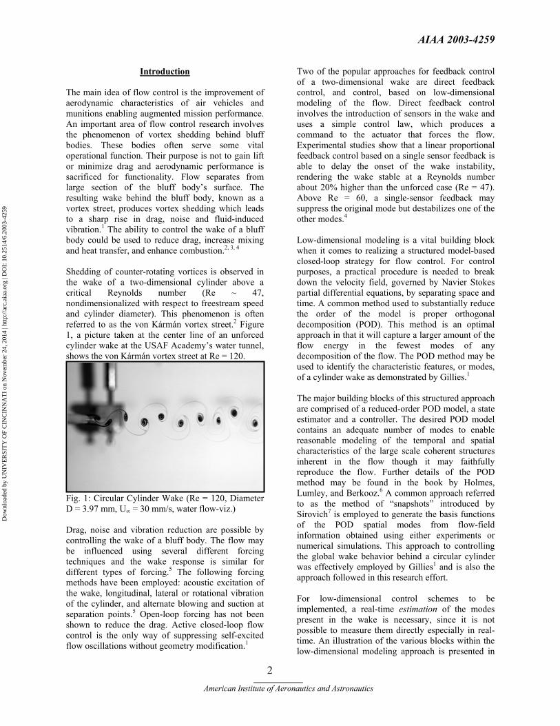
The main idea of flow control is the improvement of aerodynamic characteristics of air vehicles and munitions enabling augmented mission performance. An important area of flow control research involves the phenomenon of vortex shedding behind bluff bodies. These bodies often serve some vital operational function. Their purpose is not to gain lift or minimize drag and aerodynamic performance is sacrificed for functionality. Flow separates from large section of the bluff body’s surface. The resulting wake behind the bluff body, known as a vortex street, produces vortex shedding which leads to a sharp rise in drag, noise and fluid-induced vibration.1 The ability to control the wake of a bluff body could be used to reduce drag, increase mixing and heat transfer, and enhance combustion.2, 3, 4 Shedding of counter-rotating vortices is observed in the wake of a two-dimensional cylinder above a critical Reynolds number (Re ~ 47, nondimensionalized with respect to freestream speed and cylinder diameter). This phenomenon is often referred to as the von Kármán vortex street.2 Figure 1, a picture taken at the center line of an unforced cylinder wake at the USAF Academy’s water tunnel, shows the von Kármán vortex street at Re = 120.

Fig. 1: Circular Cylinder Wake (Re = 120, Diameter D = 3.97 mm, U∞ = 30 mm/s, water flow-viz.)

Drag, noise and vibration reduction are possible by controlling the wake of a bluff body. The flow may be influenced using several different forcing techniques and the wake response is similar for different types of forcing.5 The following forcing methods have been employed: acoustic excitation of the wake, longitudinal, lateral or rotational vibration of the cylinder, and alternate blowing and suction at separation points.5 Open-loop forcing has not been shown to reduce the drag. Active closed-loop flow control is the only way of suppressing self-excited flow oscillations without geometry modification.1

Two of the popular approaches for feedback control of a two-dimensional wake are direct feedback control, and control, based on low-dimensional modeling of the flow. Direct feedback control involves the introduction of sensors in the wake and uses a simple control law, which produces a command to the actuator that forces the flow. Experimental studies show that a linear proportional feedback control based on a single sensor feedback is able to delay the onset of the wake instability, rendering the wake stable at a Reynolds number about 20% higher than the unforced case (Re = 47). Above Re = 60, a single-sensor feedback may suppress the original mode but destabilizes one of the other modes.4 Low-dimensional modeling is a vital building block when it comes to realizing a structured model-based closed-loop strategy for flow control. For control purposes, a practical procedure is needed to break down the velocity field, governed by Navier Stokes partial differential equations, by separating space and time. A common method used to substantially reduce the order of the model is proper orthogonal decomposition (POD). This method is an optimal approach in that it will capture a larger amount of the flow energy in the fewest modes of any decomposition of the flow. The POD method may be used to identify the characteristic features, or modes, of a cylinder wake as demonstrated by Gillies.1

The major building blocks of this structured approach are comprised of a reduced-order POD model, a state estimator and a controller. The desired POD model contains an adequate number of modes to enable reasonable modeling of the temporal and spatial characteristics of the large scale coherent structures inherent in the flow though it may faithfully reproduce the flow. Further details of the POD method may be found in the book by Holmes, Lumley, and Berkooz.6 A common approach referred to as the method of “snapshots” introduced by Sirovich7 is employed to generate the basis functions of the POD spatial modes from flow-field information obtained using either experiments or numerical simulations. This approach to controlling the global wake behavior behind a circular cylinder was effectively employed by Gillies1 and is also the approach followed in this research effort.

For low-dimensional control schemes to be implemented, a real-time estimation of the modes present in the wake is necessary, since it is not possible to measure them directly especially in real-time. An illustration of the various blocks within the low-dimensional modeling approach is presented in

Dow

nloa

ded

by U

NIV

ER

SIT

Y O

F C

INC

INN

AT

I on

Nov

embe

r 24

, 201

4 | h

ttp://

arc.

aiaa

.org

| D

OI:

10.

2514

/6.2

003-

4259

AIAA 2003-4259


3

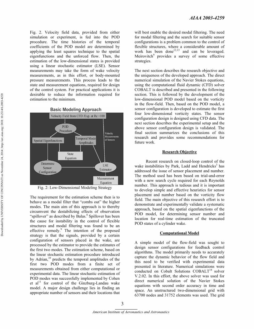
Fig. 2. Velocity field data, provided from either simulation or experiment, is fed into the POD procedure. The time histories of the temporal coefficients of the POD model are determined by applying the least squares technique to the spatial eigenfunctions and the unforced flow. Then, the estimation of the low-dimensional states is provided using a linear stochastic estimator (LSE). Sensor measurements may take the form of wake velocity measurements, as in this effort, or body-mounted pressure measurements. This process leads to the state and measurement equations, required for design of the control system. For practical applications it is desirable to reduce the information required for estimation to the minimum.

Fig. 2: Low-Dimensional Modeling Strategy

The requirement for the estimation scheme then is to behave as a modal filter that “combs out” the higher modes. The main aim of this approach is to thereby circumvent the destabilizing effects of observation “spillover” as described by Balas.8 Spillover has been the cause for instability in the control of flexible structures and modal filtering was found to be an effective remedy.9 The intention of the proposed strategy is that the signals, provided by a certain configuration of sensors placed in the wake, are processed by the estimator to provide the estimates of the first two modes. The estimation scheme, based on the linear stochastic estimation procedure introduced by Adrian,10 predicts the temporal amplitudes of the first two POD modes from a finite set of measurements obtained from either computational or experimental data. The linear stochastic estimation of POD modes was successfully implemented by Cohen et al11 for control of the Ginzburg-Landau wake model. A major design challenge lies in finding an appropriate number of sensors and their locations that

will best enable the desired modal filtering. The need for modal filtering and the search for suitable sensor configurations is a problem common to the control of flexible structures, where a considerable amount of work has been done12,13 and can be leveraged. Meirovitch9 provides a survey of some effective strategies. The next section describes the research objective and the uniqueness of the developed approach. The direct numerical simulation of the Navier Stokes equations, using the computational fluid dynamic (CFD) solver COBALT is described and presented in the following section. This is followed by the development of the low-dimensional POD model based on the vorticity in the flow-field. Then, based on the POD model, a sensor configuration is developed to estimate the first four low-dimensional vorticity states. The sensor configuration design is designed using CFD data. The next section describes the experimental setup and the above sensor configuration design is validated. The final section summarizes the conclusions of this research and provides some recommendations for future work.

Research Objective

Recent research on closed-loop control of the

wake instabilities by Park, Ladd and Hendricks3 has addressed the issue of sensor placement and number. The method used has been based on trial-and-error with a new search cycle required for each Reynolds number. This approach is tedious and it is important to develop simple and effective heuristics for sensor placement and number based on the vorticity flow field. The main objective of this research effort is to demonstrate and experimentally validate a systematic approach, based on the spatial eigenfunctions of the POD model, for determining sensor number and location for real-time estimation of the truncated POD states of a cylinder wake.

Computational Model A simple model of the flow-field was sought to design sensor configurations for feedback control algorithms. The model primarily needs to accurately capture the dynamic behavior of the flow field and this need to be verified with experimental data presented in literature. Numerical simulations were conducted on Cobalt Solutions COBALT14 solver V.2.02. In this effort, the above solver was used for direct numerical solution of the Navier Stokes equations with second order accuracy in time and space. An unstructured two-dimensional grid with 63700 nodes and 31752 elements was used. The grid

Dow

nloa

ded

by U

NIV

ER

SIT

Y O

F C

INC

INN

AT

I on

Nov

embe

r 24

, 201

4 | h

ttp://

arc.

aiaa

.org

| D

OI:

10.

2514

/6.2

003-

4259

AIAA 2003-4259


4

extended from –16.9 cylinder diameters to 21.1 cylinder diameters in the x (streamwise) direction, and ±19.4 cylinder diameters in y (flow normal) direction. Additional simulation parameters are as follows: • Two-dimensional cylinder, diameter = 1m • Reynolds Number (Re) = 100 • Laminar Navier-Stokes equations • Vortex shedding frequency – 5.55Hz. • Mean flow, U= 34 m/s • Damping Coefficients: Advection = 0.01;

Diffusion = 0.00 • 32 Iterations for matrix solution scheme • 3 Newtonian sub-iterations • Non-dimensional time step, ∆t*=∆t.U/D= 0.05 • Time step, ∆t = 0.00147 s.

The simulation was triggered by skewing the incoming mean flow by α = 0.5 degrees to introduce an initial perturbation. An important issue concerning the validity of the CFD model needs to be addressed before using the data. For validation of the unforced cylinder wake CFD model at Re = 100, the resulting value of the mean drag coefficient, Cd, will be compared to experimental and computational investigations reported in the literature. At Re = 100, experimental data, reported by Oertel15 and Panton16 point to Cd values from 1.26 to 1.4. Furthermore, Min and Choi17 report on several numerical studies that obtained drag coefficients of 1.35 and 1.337. The COBALT CFD model, used in this effort results in a Cd =1.35 at Re = 100, which compares well with the reported literature. Another important benchmark parameter concerns the value of the non-dimensional Strouhal number (St) for the unforced cylinder wake. Experimental results at Re = 100, presented by Williamson,18 point to St values ranging from 0.163 and 0.166. The COBALT CFD model, used in this effort, has a St = 0.163 at Re = 100 which also compares well with the reported literature.

POD Modeling

Feasible real time estimation and control of the cylinder wake may be effectively realized by reducing the model complexity of the cylinder wake as described by the Navier-Stokes equations, using POD techniques. POD, a non-linear model reduction approach is referred to in the literature as the Karhunen-Loeve expansion.6 The desired POD model will contain an adequate number of modes to enable modeling of the temporal and spatial characteristics of the large-scale coherent structures inherent in the flow, but no more modes than necessary.

In this effort, the basis functions of the POD spatial modes from the numerical solution of the Navier-Stokes equations obtained using COBALT.14 In all 70 snap-shots were used equally spaced at 0.00735 seconds apart. The time between snapshots is five times the simulation time step. The snap-shots were taken after ensuring that the cylinder wake reached steady state. Only the U velocity component (in the direction of the mean flow) was used for the sensor placement and number studies reported in this effort. For control design purposes, the POD method enables the Navier-Stokes equations to be modeled as a set of ordinary differential equations (O.D.E.).19 The POD analysis was completed in MATLAB. At first, the vorticity data is loaded and arranged from the COBALT solver of the Navier-Stokes equations for the circular cylinder wake at Re = 100. The decomposition of this component of the velocity field is as follows: ),,(),(),,(~ tyxuyxUtyxu += (1) where U[m/s] denotes the mean flow and u[m/s] is the fluctuating component that may be expanded as:

∑=

=n

k

kik yxtatyxu

1

)( ),()(),,( φ (2)

where ak(t) denotes the time-dependent coefficients having units of m/s (see Fig. 3) and фi(x,y) represents the non-dimensional spatial eigenfunctions (see Fig. 4) determined from the POD procedure. In this entire effort, the velocity component represents the vorticity, which is calculated from the flow field. From an ensemble of snapshots, the 'average snapshot' is computed and then this profile is subtracted from each member of the ensemble. This is done mainly for reasons of scale; i.e. the deviations from the mean contain information of interest but may be small compared with the original signal. Next, the empirical correlation matrix, R is computed. A simple approximation technique is applied to obtain the numerical integration. In this effort, the correlation matrix is computed using the inner product.19 Solving the eigenvalue problem, the eigenvalues and the orthogonal spatial eigenfunctions, фi(x,y) are obtained (see Fig. 3). Since the eigenvalues measure the relative energy of the system dynamics contained in that particular mode, they may be normalized to correspond to a percentage. Finally, the time histories of the

Dow

nloa

ded

by U

NIV

ER

SIT

Y O

F C

INC

INN

AT

I on

Nov

embe

r 24

, 201

4 | h

ttp://

arc.

aiaa

.org

| D

OI:

10.

2514

/6.2

003-

4259

AIAA 2003-4259


5

temporal coefficients of the POD model, ak(t), are determined using the extracted spatial modes and the data of the unforced flow. For an arbitrarily forced circular cylinder, we can write the low-dimensional wake model20 as:

aknkk fbag

dtda

+= )( (3)

where gk, for k modes, is a quadratic non-linear function of the time-dependent mode coefficients. bk are coefficients associated with the control input and fa is the feedback control input to the cylinder. For the open-loop case fa = 0. For a full state feedback system, the closed loop control input, fa, is a function of ak. However, it is not possible to obtain a direct measurement of ak. The POD algorithms, based on the above steps and realized in MATLAB, were applied to the CFD and experimental data obtained at Re = 100 and Re = 108 respectively. The energy content for the first eight vorticity modes is presented in Table 1. It can be seen that most of the kinetic energy of the flow lies in the first eight modes. An important aspect of reduced order modeling concerns truncation. How many modes are important and what are the criteria for effective truncation?

The answers to the above questions have been addressed by Cohen et al.20 This effort showed that control of the POD model of the von Kármán vortex street in the wake of a circular cylinder at Re = 100 is enabled using just the first mode. Furthermore, feedback based on the first mode alone suppressed all the other modes in the four mode POD model. In view of this result, truncation of the POD model will take place after the first four modes, which contain 94.4% of the total amount of energy. At this point, it is imperative to note the difference between the number of modes required to reconstruct the flow and the number of modes required for effective low-dimensional modeling for control design. In this effort, we are interested in estimating only those modes required for closed-loop control. On the other hand, an accurate reconstruction of the velocity field based on a low-dimensional model may be obtained using between 4-8 modes.19 The POD algorithm was applied to the velocity component in the direction of the flow as described in Equation (1). The velocity field may be obtained from a CFD simulation or from a real-time PIV (particle image velocimetry) system as described by Siegel et al.21 The quintessential question is whether an effective estimate of the states, of the 4 mode low-dimensional model, ak, can be estimated based on the real-time velocity field

measurements. The answer is in the affirmative and the details that provides the estimate of the first four modes, a1-a4, are presented in the next section.

Estimation and Sensor Configuration The time histories of the temporal coefficients of the POD model are determined by applying the least squares technique to the spatial modes and the unforced flow. The intent of the proposed strategy is that the velocity measurements provided by the sensors are processed by the estimator to provide the estimates of the first two temporal modes. The estimation scheme, based on the linear stochastic estimation procedure introduced by Adrian,10 predicts the temporal amplitudes of the first four POD modes (about 95% of the kinetic energy) from a finite set of velocity measurements obtained from the CFD solution of the uncontrolled cylinder wake. For each sensor configuration, 70 velocity measurements were used equally spaced at 0.00735 seconds apart. All the measurements were taken after ensuring that the cylinder wake reached steady state. Only data concerning velocity components in the direction of the flow were used for the sensor placement and number studies reported in this effort. The vorticity mode amplitudes, a1-a4, presented in Fig. 4 at the above 70 discrete times were mapped onto the extracted sensor signals, us, as follows:

∑=

=m

ss

nsn tuCta

1)()( (4)

where m is the number of sensors and Cns represents

the coefficients of the linear mapping. The effectiveness of a linear mapping between for velocity measurements and POD states has been experimentally validated by Siegel et al. 23 The coefficients Cn

s (n=1,2; s=1,m) in Equation (4) are obtained via the linear stochastic estimation method from the set of discrete sensor signals and temporal mode amplitudes. For the sensor configuration, the effectiveness of the linear stochastic estimation process for the estimation of the first four temporal mode amplitudes, a1 – a4, is calculated. The quantitative criterion, associated with estimation accuracy, is based on the root mean square (RMS) of the error between the estimated and the extracted mode amplitudes. For sake of convenience, this RMS error is normalized with the RMS of the desired extracted mode amplitudes, and presented as a percentage. The resulting error percentage and the number of sensors may be integrated together into a cost function and the purpose of the design process would then be to select the configuration that minimizes this cost.

Dow

nloa

ded

by U

NIV

ER

SIT

Y O

F C

INC

INN

AT

I on

Nov

embe

r 24

, 201

4 | h

ttp://

arc.

aiaa

.org

| D

OI:

10.

2514

/6.2

003-

4259

AIAA 2003-4259


6

−1 0 1 2 3 4 5 6−2

−1.5

−1

−0.5

0

0.5

1

1.5

X/D

Y/D

Mode 1

−1 0 1 2 3 4 5 6−2

−1.5

−1

−0.5

0

0.5

1

1.5

X/D

Y/D

Mode 2

−1 0 1 2 3 4 5 6−2

−1.5

−1

−0.5

0

0.5

1

1.5

X/D

Y/D

Mode 3

−1 0 1 2 3 4 5 6−2

−1.5

−1

−0.5

0

0.5

1

1.5

X/D

Y/D

Mode 4

−1 0 1 2 3 4 5 6 7−2

−1.5

−1

−0.5

0

0.5

1

1.5

X/D

Y/D

Mode 1

−1 0 1 2 3 4 5 6 7−2

−1.5

−1

−0.5

0

0.5

1

1.5

X/D

Y/D

Mode 2

−1 0 1 2 3 4 5 6 7−2

−1.5

−1

−0.5

0

0.5

1

1.5

X/D

Y/D

Mode 3

−1 0 1 2 3 4 5 6 7−2

−1.5

−1

−0.5

0

0.5

1

1.5

X/D

Y/D

Mode 4

Fig. 3: Spatial Eigenfunctions of 4 mode model. The left column contains the eigenfuctions obtained from CFD data at Re=100, and the right column contains the eigenfuctions obtained from Experimental data at Re=108. Solid lines are positive, dashed lines are negative isocontours.

Dow

nloa

ded

by U

NIV

ER

SIT

Y O

F C

INC

INN

AT

I on

Nov

embe

r 24

, 201

4 | h

ttp://

arc.

aiaa

.org

| D

OI:

10.

2514

/6.2

003-

4259

AIAA 2003-4259


7

Table 1: Energy content (eigenvalues) for the first eight vorticity modes of the POD model

Mode I Mode II Mode III Mode IV Mode V Mode VI Mode VII Mode VIII CFD Data

Re = 100 [%]

46.17

37.82

5.47

4.94

2.31

2.26

0.35

0.34 Experimental

Data Re = 108 [%]

43.40

41.98

3.03

2.73

0.79

0.70

0.35

0.30

2.4 2.5 2.6 2.7 2.8 2.9 3 3.1 3.2−100

−80

−60

−40

−20

0

20

40

60

80

100

Time [s]

Vor

ticity

Mod

e A

mpl

itude

s

CFD Data Re =100

Ext. Mode 1Ext. Mode 2Ext. Mode 3Ext. Mode 4Est. Mode 1Est. Mode 2Est. Mode 3Est. Mode 4

Fig. 4: Extracted Mode Amplitudes projected on the estimated ones for CFD data at Re=100

Closed-loop flow control is a relatively new research field and the issue of sensor placement and number has been dealt with in an ad-hoc manner. In this effort, an attempt will be made to emulate some of the proven successes form the field of structural structure control. Heuristically speaking, when some very fine dust particles are placed on a flexible plate, excited at one of its natural frequencies, after a short while the particles arrange themselves in a certain pattern typical of those frequencies. The particles will be concentrated in the areas that do not experience any motion (the nodes). On the other hand, at the areas where the motion is most

active (the internodes) will be clean of particles. It is at the internodes that the vibrational energy of that particular mode is at a maximum and sensors placed at these locations are extremely effective in estimating that particular mode. The above heuristic approach has been used by Bayon de Noyer22 in locating effective sensor locations for acceleration feedback control to alleviate tail buffeting of a high performance twin tail aircraft. Note the usage of the term “effective sensor configuration” as it is based on validated heuristics as opposed to “optimal sensor

Dow

nloa

ded

by U

NIV

ER

SIT

Y O

F C

INC

INN

AT

I on

Nov

embe

r 24

, 201

4 | h

ttp://

arc.

aiaa

.org

| D

OI:

10.

2514

/6.2

003-

4259

AIAA 2003-4259


8

configuration” that results from a mathematical pattern search for a sensor configuration. So, what needs to be done to determine an effective sensor configuration is to find the areas of energetic modal activity. Table 2: Location of vorticity maxima/minima of the spatial eigenfunctions used for sensor placement

X/D Y/D Mode 1

1. 2.

2.0 4.0

0.0 0.0

Mode 2 3. 4.

1.5 3.0

0.0 0.0

Mode 3 5. 6. 7. 8.

2.2 2.3 3.3 3.3

-0.3 0.3 -0.6 0.6

Mode 4 5. 6. 7. 8.

2.8 2.8 3.8 3.8

0.5 -0.5 0.8 -0.8

The spatial eigenfunctions obtained from the POD procedure provides information concerning the location of areas where modal activity is at its highest. In Fig. 3, these energetic areas would be the maxima (solid lines in Fig. 3) and minima (dashed lines in Fig. 3). Placing sensors at the energetic maxima and minima of each mode is the basic hypothesis of this effort and the purpose of the CFD simulation is to design a sensor configuration which is later validated using water-tunnel experiments. Location of vorticity maxima/minima of the spatial eigenfunctions (see Fig. 3) are used for sensor placement as shown in Table 2. The locations of the sensors in Table 2 are referenced in terms of the coordinates, non-dimensionalized with respect to the cylinder diameter D, namely, X/D and Y/D. A sensor was placed on each the maxima and the minima of modes 1 and 2 (see Fig. 3). On the other hand, for effective estimation, two pairs of sensors each are located on maxima/minima of modes 3 and 4. The estimated versus desired mode amplitude plot, for the above sensor configuration is presented in Fig. 4. For this configuration, the RMS estimation errors are provided in Table 3. Considering the fact that the LSE is providing vorticity estimates, the RMS values in Table 3 are low and can be dealt with using a moderately robust controller.

Experimental Set Up and Validation

The basis for validation of the design concerning sensor configuration was experimentally obtained from velocity measurements in the wake of a circular cylinder at Re =

108. The experimental measurements were obtained in the Eidetic Model 2436 recirculating water tunnel. The water tunnel is situated in the Aeronautics Laboratory at the US Air Force Academy. The cross section of the water tunnel is 38 cm × 38 cm and the test section is 1.5m in length. The circular cylinder model, as depicted in Fig. 6, is comprised of a stainless steel rod, has a diameter, D, of 3.97 mm and a span, L, of 381 mm. The aspect ratio of the cylinder, L/D, is about 95. The cylinder was positioned horizontally in the water tunnel. The actuation system shown in Fig. 6 was not used for the unforced experiments in this effort. The Reynolds number (Re = U∞D/υ) is calculated from the freestream velocity, U∞, obtained from PIV (particle image velocimetry) velocity measurements. The kinematic viscosity, υ, is calculated on the basis of temperature measurements. The natural shedding frequency of the cylinder, f, was calculated from the period of the time dependent mode amplitude, a1, as shown in Fig. 5. The calculated Strouhal number (St = fD/U∞) was then obtained based on the shedding frequency calculation. Williamson18 provides experimental data that correlates the Reynolds number to the Strouhal number for a circular cylinder and this information is used to obtain the expected Strouhal number. In Table 4, the expected and the calculated Strouhal numbers are compared. Furthermore, an uncertainty analysis provides a Reynolds number accuracy of ±7.5 (or 6-7% error). The superposition of the percent difference presented in Table 4 on the data provided by Williamson18 validates the experimental working point at a Reynolds number of 108.

Fig. 5: Experimental Circular Cylinder Model The digital PIV system provided two-dimensional velocity field measurements in the wake of the unforced cylinder from which the vorticity was calculated. The

Dow

nloa

ded

by U

NIV

ER

SIT

Y O

F C

INC

INN

AT

I on

Nov

embe

r 24

, 201

4 | h

ttp://

arc.

aiaa

.org

| D

OI:

10.

2514

/6.2

003-

4259

AIAA 2003-4259


9

field of view extended from the trailing edge of the cylinder to approximately eight diameters (8D) downstream. The PIV system employed a 1 Mpixel CCD camera. It was operated in dual exposure mode using cross correlation to determine the pixel displacements based on two snapshots. A 32×32 pixel interrogation area with 50% overlap was used in the data reduction. This setup results in vector field of 49 x 49 vectors. The field has a spatial resolution of -3.6 < X/D < 7.8. Each vector map was post-processed using a two-step sequence: first, a validation routine examined a 5×5 vector area and

replaced rejected vectors with an averaged estimate; second, an averaging filter was applied to each 5×5 vector area to reduce noise. The rejection criterion was determined as a vector being more than 10% different in magnitude than the surrounding vectors average. An invalid vector is one that does not accurately capture the velocity information at a point in the flow field. Vectors making the above criteria were replaced by the mean of their neighbors.

9.5 10 10.5 11 11.5 12 12.5 13 13.5−0.06

−0.04

−0.02

0

0.02

0.04

0.06

Time [s]

Vor

ticity

Mod

e A

mpl

itude

s

Ext. Mode 1Ext. Mode 2Ext. Mode 3Ext. Mode 4Est. Mode 1Est. Mode 2Est. Mode 3Est. Mode 4

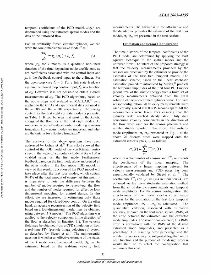
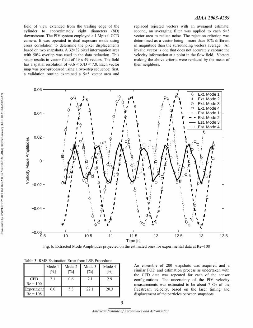
Fig. 6: Extracted Mode Amplitudes projected on the estimated ones for experimental data at Re=108 Table 3: RMS Estimation Error from LSE Procedure

Mode 1 [%]

Mode 2 [%]

Mode 3 [%]

Mode 4 [%]

CFD Re = 100

2.1 0.6 7.1 2.9

Experiment Re = 108

6.0 5.3 22.1 20.3

An ensemble of 200 snapshots was acquired and a similar POD and estimation process as undertaken with the CFD data was repeated for each of the sensor configurations. The uncertainty of the PIV velocity measurements was estimated to be about 7-8% of the freestream velocity, based on the laser timing and displacement of the particles between snapshots.

Dow

nloa

ded

by U

NIV

ER

SIT

Y O

F C

INC

INN

AT

I on

Nov

embe

r 24

, 201

4 | h

ttp://

arc.

aiaa

.org

| D

OI:

10.

2514

/6.2

003-

4259

AIAA 2003-4259


10

From Fig. 6, it can be seen that the sensor configuration, detailed in Table 2, brings the r.m.s of the estimation error to 5-6% for the first two modes and to about 20% of modes 3-4. This error should be acceptable for a moderately robust controller. Given the velocity measurement error of 7-8%, it seems that the above results, especially for modes 1-2, are fairly decent.

Table 4: Validation of the data (Re vs. St) Reynolds

Number Expected Strouhal

Number18

Observed Strouhal Number

Percent Difference

[%] CFD

Re = 100 100 0.165 0.163 1.2

Experiment Re = 108

108 0.168 0.160 4.8

The vorticity signals (u), provided by a certain configuration of sensors, are processed by the estimator to provide the estimates of the first 4 modes. The estimation scheme, based on the linear stochastic estimation procedure, predicts the temporal amplitudes of the first 4 POD modes from a finite set of measurements obtained from CFD/experimental data. The coefficients Cn

s in Equation (4) are obtained via the linear stochastic estimation method from the set of discrete snapshots (200 for experiments and 70 for CFD simulation). This procedure is done off-line just once for each case.

Conclusions and Recommendations

A heuristic procedure was developed to determine the placement and number of sensors for the feedback control suppression of the wake instability behind a circular cylinder. This procedure is based on a low-dimensional, proper orthogonal decomposition modeling and linear stochastic estimation. The development of the procedure was based on COBALT CFD simulations of a cylinder at a Reynolds number of 100. Experimental studies, based on noisy experimental data obtained from the water tunnel cylinder model at a Reynolds number of 108, validated the effectiveness of the developed sensor placement and design procedure. Results show that for experimental data, the root mean square estimation error of the estimates of the first 2 modes was within 6% and for the next 2 modes was within 20%. This level of error is acceptable for a moderately robust controller. Further research will aim at refining the developed heuristic procedure for sensor number and placement by taking symmetry, with respect to the x-axis, into account. In this effort, we noticed the potential for estimation error improvement by placing sensors at maxima/minima of the spatial eigenfunctions of modes 1-4. This potential

should be further examined in a sensitivity study. Furthermore, there may be additional cost improvements to be gained by implementing a non-linear estimator instead of the linear stochastic estimator. It will be beneficial to examine the generic nature of the developed strategy for different bluff body geometries and Reynolds numbers.

Acknowledgements

The first author would like to acknowledge the support provided by the AFOSR/ESEP program. The authors would like to acknowledge the support and assistance provided by Dr. Belinda King (AFOSR). The authors would like to thank cadets John Dayton and Kevin Hoy for collecting the experimental data in the water tunnel and Major Jim Forsythe for providing the CFD model.

References

1Gillies, E. A., “Low-dimensional Control of the

Circular Cylinder Wake”, Journal of Fluid Mechanics, Vol. 371, 1998, 157-178.

2von Kármán, T., “Aerodynamics: Selected Topics in Light of their Historic Development”, Cornell University Press, Ithaca, New York, 1954.

3Park, D.S., Ladd, D.M., and Hendricks, E.W., “Feedback Control of a Global Mode in Spatially Developing Flows”, Physics Letters A, Vol. 182, 1993, pp. 244-248.

4Roussopoulos, K., “Feedback Control of Vortex Shedding at Low Reynolds Numbers”, Journal of Fluid Mechanics, Vol. 248, 1993, pp. 267-296.

5Blevins. R. “Flow Induced Vibration”, 2nd Edition, Van Nostrand Reinhold, New York, 1990.

6Holmes, P., Lumley, J.L., and Berkooz, G., “Turbulence, Coherent Structures, Dynamical Systems and Symmetry”, Cambridge University Press, Cambridge, 1996.

7Sirovich, L., “Turbulence and the Dynamics of Coherent Structures Part I: Coherent Structures”, Quarterly of Applied Mathematics, Vol. 45, No. 3, 1987, pp. 561-571. 8Balas, M.J., “Active Control of Flexible Systems”, Journal of Optimization Theory and Applications, Vol. 25, No. 3, 1978, pp. 217-236. 9Meirovitch, L., “Dynamics and Control of Structures”, John Wiley & Sons, Inc., New York, 1990, pp. 313-351. 10Adrian, R.J., “On the Role of Conditional Averages in Turbulence Theory”, Proceedings of the Fourth Biennial Symposium on Turbulence in Liquids, J. Zakin and G. Patterson (Eds.), Science Press, Princeton, 1977, pp. 323-332. 11Cohen, K., Siegel S., McLaughlin T., and Myatt J., 2003, "Proper Orthogonal Decomposition Modeling Of

Dow

nloa

ded

by U

NIV

ER

SIT

Y O

F C

INC

INN

AT

I on

Nov

embe

r 24

, 201

4 | h

ttp://

arc.

aiaa

.org

| D

OI:

10.

2514

/6.2

003-

4259

AIAA 2003-4259


11

A Controlled Ginzburg-Landau Cylinder Wake Model", AIAA Paper 2003-1292, Jan. 2003. 12Baruh, H., and Choe, K., "Sensor Placement in Structural Control", Journal of Guidance and Control, Volume 13, Number 3, May-June 1990, pp. 524-533. 13Lim, K.B., “A Disturbance Rejection Approach to Actuator and Sensor Placement”, NASA CR-201623, Jan-Feb.1997. 14Cobalt CFD, Cobalt Solutions, LLC, URL: http://www.cobaltcfd.com [cited 14 February 2003]. 15Oertel, H. Jr., “Wakes Behind Blunt Bodies”, Annual Review of Fluid Mechanics, Vol. 22, 1990, pp. 539-564. 16Panton, R.L., “Incompressible Flow”, 2nd Edition, John Wiley & Sons, New York, 1996, pp. 384-400. 17Min, C., and Choi, H., “Suboptimal Feedback Control of Vortex Shedding at Low Reynolds Numbers”, Journal of Fluid Mechanics, Vol. 401, 1999, pp.123-156. 18Williamson, C. H. K., “Vortex Dynamics in the Cylinder Wake”, Annual Review of Fluid Mechanics, Vol. 28, 1996, pp. 477-539.

19Smith, D. R., Siegel, S., and McLaughlin T., “Modeling of the wake Behind a Circular Cylinder Undergoing Rotational Oscillation”, AIAA Paper 2002-3066, June 2002.

20Cohen, K., Siegel, S., McLaughlin, T., and Gillies, E., “Feedback Control of a Cylinder Wake Low-Dimensional Model”, AIAA Journal, Vol. 41, No. 8, August 2003 (tentative). 21Siegel, S., Cohen, K., McLaughlin, T., and Myatt, J., "Real-Time Particle Image Velocimetry for Closed-Loop Flow Control Studies", AIAA Paper 2003-0920, Jan. 2003. 22Bayon de Noyer, “Tail Buffet Alleviation of High Performance Twin Tail Aircraft using Offset Piezoceramic Stack Actuators and Acceleration Feedback Control”, Ph.D. Thesis, Aerospace Engineering, Georgia Institute of Technology, Atlanta, Georgia 30332, November 1999. 23Siegel, S., Cohen, K., Smith, D., and McLaughlin, T, "Observability Conditions for POD Modes in a Circular Cylinder Wake", 55th APS/DFD Meeting, Vol. 47, No. 10, Paper DN 4, Dallas, TX, Nov. 2002.

Dow

nloa

ded

by U

NIV

ER

SIT

Y O

F C

INC

INN

AT

I on

Nov

embe

r 24

, 201

4 | h

ttp://

arc.

aiaa

.org

| D

OI:

10.

2514

/6.2

003-

4259