arX

iv:1

006.

0653

v1 [

hep-

ph]

3 J

un 2

010

Preprint typeset in JHEP style - HYPER VERSION SLAC-PUB-14136

June 3, 2010

RECO level√smin

and subsystem√smin

: improved

global inclusive variables for measuring the new physics

mass scale in 6ET events at hadron colliders

Partha Konar

Physics Department, University of Florida, Gainesville, FL 32611, USA

E-mail: konar@phys.ufl.edu

Kyoungchul Kong

Theoretical Physics Department, SLAC, Menlo Park, CA 94025, USA

E-mail: kckong@slac.stanford.edu

Konstantin T. Matchev

Physics Department, University of Florida, Gainesville, FL 32611, USA

E-mail: matchev@phys.ufl.edu

Myeonghun Park

Physics Department, University of Florida, Gainesville, FL 32611, USA

E-mail: ishaed@phys.ufl.edu

Abstract: The variable√smin was originally proposed in [1] as a model-independent, global

and fully inclusive measure of the new physics mass scale in missing energy events at hadron

colliders. In the original incarnation of√smin, however, the connection to the new physics

mass scale was blurred by the effects of the underlying event, most notably initial state

radiation and multiple parton interactions. In this paper we advertize two improved variants

of the√smin variable, which overcome this problem. First we show that by evaluating the√

smin variable at the RECO level, in terms of the reconstructed objects in the event, the

effects from the underlying event are significantly diminished and the nice correlation between

the peak in the√s(reco)min distribution and the new physics mass scale is restored. Secondly,

the underlying event problem can be avoided altogether when the√smin concept is applied

to a subsystem of the event which does not involve any QCD jets. We supply an analytic

formula for the resulting subsystem√s(sub)min variable and show that its peak exhibits the

usual correlation with the mass scale of the particles produced in the subsystem. Finally,

we contrast√smin to other popular inclusive variables such as HT , MTgen and MTTgen. We

illustrate our discussion with several examples from supersymmetry, and with dilepton events

from top quark pair production.

Keywords: Beyond Standard Model, Hadronic Colliders, Supersymmetry Phenomenology.

Contents

1. Introduction and motivation 1

1.1 The need for a universal, global and inclusive mass variable 1

1.2 Definition of√smin 4

1.3√smin and the underlying event problem 6

2. Definition of the RECO level variable√s(reco)min 7

3. Definition of the subsystem variable√s(sub)min 10

4. SM example: dilepton events from tt production 13

4.1 Event simulation details 13

4.2√s(reco)min variable 14

4.3√s(sub)min variable 20

5. An exclusive SUSY example: multijet events from gluino production 23

6. An inclusive SUSY example: GMSB study point GM1b 27

7. Comparison to other inclusive collider variables 31

8. Summary and conclusions 35

1. Introduction and motivation

1.1 The need for a universal, global and inclusive mass variable

It is generally believed that missing energy signatures offer the best bet for discovering new

physics Beyond the Standard Model (BSM) at colliders. This belief is reinforced by the dark

matter puzzle - the Standard Model (SM) does not contain a suitable dark matter candidate.

If dark matter particles are produced at colliders, they will be invisible in the detector,

and will in principle lead to missing energy and missing momentum. However, at hadron

colliders the total energy and longitudinal momentum of the event are unknown. Therefore,

the production of any invisible particles can only be inferred from an imbalance in the total

transverse momentum. The measured missing transverse momentum 6~PT then gives the sum

of the transverse momenta of all invisible particles in the event.

Unfortunately, 6 ~PT is the only measured quantity directly related to the invisible parti-

cles. Without any further model-dependent assumptions, it is in general very difficult if not

– 1 –

impossible to make any definitive statements about the nature and properties of the miss-

ing particles. For example, leaving all theoretical prejudice aside, one would not be able to

answer such basic and fundamental questions like [1–5]: How many invisible particles were

produced in the event? Are all invisible particles SM neutrinos, or are there any new neutral,

stable, weakly-interacting massive particles (WIMPs) among them? What are the masses

of the new invisible particles? What are their spins? What are the masses of any (parent)

particles which may have decayed to invisible particles?

The recent literature is abundant with numerous proposals1 on how under particular cir-

cumstances one might be able to measure the masses of the invisible particles. Unfortunately,

all of the proposed methods suffer from varying degrees of model-dependence2:

• Limited applicability topology-wise. Most methods are model-dependent in the sense

that each method crucially relies on the assumption of a very specific event topology.

One common flaw of all methods on the market is that they usually do not allow any

SM neutrinos to enter the targeted event topology, and the missing energy is typically

assumed to arise only as a result of the production of (two) new dark matter parti-

cles. Furthermore, each method has its own limitations. For example, the traditional

invariant mass endpoint methods [10–20] require the identification of a sufficiently long

cascade decay chain, with at least three successive two-body decays [21]. The polyno-

mial methods of Refs. [22–29] also require such long decay chains and furthermore, the

events must be symmetric, i.e. must have two identical decay chains per event, or else

the decay chain must be even longer [21]. The recently popular MT2 methods [30–39]

do not require long decay chains [21], but typically assume that the parent particles are

the same and decay to two identical invisible particles3. The limitations of the MCT

methods [40–42] are rather similar. The kinematic cusp method [43] is limited to the

so called “antler” event topology, which contains two symmetric one-step decay chains

originating from a single s-channel resonance. In light of all these various assumptions,

it is certainly desirable to have a universal method which can be applied to any event

topology. To the best of our knowledge, the only such method in the literature is the

one proposed in Ref. [1], where the√smin variable was first introduced. The

√smin

variable is defined in terms of the total energy E and 3-momentum ~P observed in the

event, and thus does not make any reference to the actual event topology. In this sense√smin is a universal variable which can be applied under any circumstances.

• Limited applicability signature-wise. As a rule, most of the proposed methods work well

only if the corresponding signature contains some minimum number of high pT isolated

leptons. Leptonic signatures have the twofold advantage of lower SM backgrounds

and good lepton momentum measurement. The performance of the methods typically

deteriorates as we lower the number of leptons in the signature. The most challenging

1See Ref. [6] for a recent review.2Worse still, there are even fewer ideas for measuring the spins of the new particles in a truly model-

independent fashion [7–9].3See [3,4] for a more general approach which avoids this assumption.

– 2 –

signature of multijets plus 6ET has rarely been studied in relation to mass and spin

measurements (see, however [33, 44–47]). Unfortunately, at hadron colliders like the

Tevatron and LHC, one typically expects strong production to dominate the new physics

cross-sections, and this in turn guarantees the presence of some minimum number of

jets in the signature. At the same time, a priori there are no theoretical arguments

which would similarly guarantee the presence of any hard isolated leptons. Therefore,

one would like to have a general, sufficiently inclusive method, which treats jets and

leptons on an equal footing. The√smin method of Ref. [1] satisfies this requirement as

well, since it does not differentiate between the type of reconstructed objects. In fact,

the original proposal of Ref. [1] did not require any object reconstruction at all, and

used (muon-corrected) calorimeter energy measurements to define the observed E and~P in the event.

• Combinatorics problem. Even if one correctly guesses the new physics event topology,

and the signature happens to be abundant in hard isolated leptons, one still has to face

the usual combinatorics problem of how to properly associate the reconstructed objects

with the individual particles in the assumed event topology. Here we shall be careful

to make the distinction between two different aspects of the combinatorics problem:

– Partitioning ambiguity. As a prototypical example, consider a model of supersym-

metry (SUSY) in which R-parity is conserved and the lightest supersymmetric

particle (LSP) is neutral and stable. Each SUSY event contains two independent

cascade decay chains, so first one must decide which reconstructed objects belong

to the first decay chain and which belong to the second [32, 48]. However, a pri-

ori there are no guiding principles on how to do this partitioning into subsets.

The decision is further complicated by the inevitable presence of jets from initial

state radiation, which have nothing to do with the SUSY cascades [49]; by final

state radiation, which modifies the assumed event topology; and by the occasional

overlapping of jets [50].

– Ordering ambiguity. Having separated the objects into two groups, one must still

decide on the sequential ordering of the reconstructed objects along each decay

chain. One well-known example of this problem is the ambiguity between the

“near” and “far” lepton in the standard jet-lepton-lepton squark decay chain [20].

The severity of either one of these two combinatorics problems depends on the type

of signature — simple signatures resulting from short decay chains suffer from less

combinatorics but tend to have larger SM backgrounds. By the same token, more

complex signatures, which result from longer decay chains, are easier to see over the

SM backgrounds, but very quickly run into severe combinatorial problems. Thus ideally

one would like to have a method which treats all objects in the event in a fully inclusive

manner, so that neither of these two combinatorial issues can ever arise at all. The√smin variable of Ref. [1] was proposed for exactly this reason, and is free of the

partitioning and ordering combinatorial ambiguities.

– 3 –

• Limited use of the available experimental information. At hadron colliders, events with

invisible particles in the final state present an additional challenge: the total energy

and longitudinal momentum of the initial state in the event are unknown. On the other

hand, the transverse momentum of the initial state is known, which has greatly moti-

vated the use of transverse variables like the missing “transverse energy” 6ET , the scalar

sum of transverse momentaHT , the transverse massMT , the stransverse massMT2 [30],

the contransverse mass MCT [40], etc. An unsettling feature of a purely transverse kine-

matical approach is that it completely ignores the measured longitudinal momentum

components of the visible particles. In principle, the longitudinal momenta also carry a

certain amount of information about the underlying physics, although it is difficult to

see immediately how this information can be utilized. (For example, one cannot take

advantage of longitudinal momentum conservation, because the longitudinal momen-

tum of the initial state is unknown.) By defining the√smin variable in a manifestly

1+3 Lorentz invariant way, Ref. [1] proposed one possible way to utilize the additional

information encoded in the measured longitudinal momenta.

The above discussion makes it clear that the method of the√smin variable has several

unique advantages over all other known methods: it is completely general and universal, is

fully inclusive, and to the fullest extent makes use of the available experimental information.

In spite of these advantages, the√smin variable has not yet found wide application. The one

major perceived drawback of√smin is its sensitivity to initial state radiation (ISR) and/or

multiple parton interactions (MPI) [1, 6, 51–53]. To see how this comes about, let us first

review the formal definition of√smin.

1.2 Definition of√smin

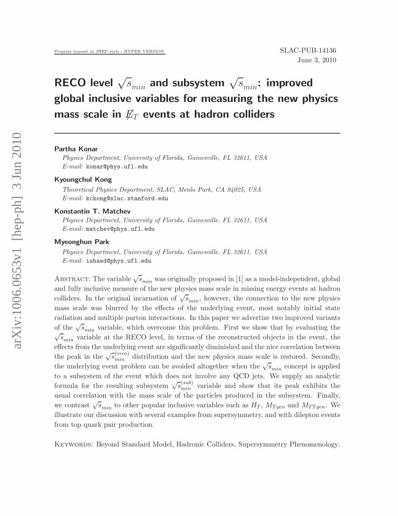
Consider the most generic missing energy event topology shown in Fig. 1. As seen from the

figure, in defining√smin, one imagines a completely general setup – each event contains some

number nvis of Standard Model (SM) particles Xi, i = 1, 2, . . . , nvis, which are visible in the

detector, i.e. their energies and momenta are in principle measured. Examples of such visible

SM particles are the basic reconstructed objects, e.g. jets, photons, electrons and muons. The

visible particles Xi are denoted in Fig. 1 with solid black lines and may originate either from

ISR, or from the hard scattering and subsequent cascade decays (indicated with the green-

shaded ellipse). In turn, the missing transverse momentum 6~PT arises from a certain number

ninv of stable neutral particles χi, i = 1, 2, . . . , ninv, which are invisible in the detector. In

general, the set of invisible particles consists of some number nχ of BSM particles (indicated

with the red dashed lines), as well as some number nν = ninv −nχ of SM neutrinos (denoted

with the black dashed lines). As already mentioned earlier, the 6~PT measurement alone does

not reveal the number ninv of missing particles, nor how many of them are neutrinos and

how many are BSM (dark matter) particles. This general setup also allows the identities and

the masses mi of the BSM invisible particles χi, (i = 1, 2, . . . , nχ) in principle to be different,

as in models with several different species of dark matter particles [54–57]. Of course, the

– 4 –

X1

X2

X3

X4

Xnvis

χninv

χnχ+2

χnχ+1

p(p)

p(p)

χnχ

χ2

χ1

E,Px, Py, Pz

6~PT

Figure 1: The generic event topology used to define the√smin variable in Ref. [1]. Black (red)

lines correspond to SM (BSM) particles. The solid lines denote SM particles Xi, i = 1, 2, . . . , nvis,

which are visible in the detector, e.g. jets, electrons, muons and photons. The SM particles may

originate either from initial state radiation (ISR), or from the hard scattering and subsequent cascade

decays (indicated with the green-shaded ellipse). The dashed lines denote neutral stable particles χi,

i = 1, 2, . . . , ninv, which are invisible in the detector. In general, the set of invisible particles consists

of some number nχ of BSM particles (indicated with the red dashed lines), as well as some number

nν = ninv −nχ of SM neutrinos (denoted with the black dashed lines). The identities and the masses

mi of the BSM invisible particles χi, (i = 1, 2, . . . , nχ) do not necessarily have to be all the same, i.e. we

allow for the simultaneous production of several different species of dark matter particles. The global

event variables describing the visible particles are: the total energy E, the transverse components Px

and Py and the longitudinal component Pz of the total visible momentum ~P . The only experimentally

available information regarding the invisible particles is the missing transverse momentum 6~PT .

neutrino masses can be safely taken to be zero

mi = 0, for i = nχ + 1, nχ + 2, . . . , ninv . (1.1)

Given this very general setup, Ref. [1] asked the following question: What is theminimum

value√smin of the parton-level Mandelstam invariant mass variable

√s which is consistent

with the observed visible 4-momentum vector Pµ ≡ (E, ~P )? As it turned out, the answer to

this question is given by the universal formula [1]

√smin(6M) ≡

√

E2 − P 2z +

√

6M2+ 6P 2T , (1.2)

– 5 –

where the mass parameter 6M is nothing but the total mass of all invisible particles in the

event:

6M ≡ninv∑

i=1

mi =

nχ∑

i=1

mi , (1.3)

and the second equality follows from the assumption of vanishing neutrino masses (1.1). The

result (1.2) can be equivalently rewritten in a more symmetric form

√smin(6M) =

√

M2 + P 2T +

√

6M2+ 6P 2T (1.4)

in terms of the total visible invariant mass M defined as

M2 ≡ E2 − P 2x − P 2

y − P 2z ≡ E2 − P 2

T − P 2z . (1.5)

Notice that in spite of the complete arbitrariness of the invisible particle sector at this point,

the definition of√smin depends on a single unknown parameter 6M - the sum of all the

masses of the invisible particles in the event. For future reference, one should keep in mind

that transverse momentum conservation at this point implies that

~PT+ 6~PT = 0. (1.6)

The main result from Ref. [1] was that in the absence of ISR and MPI, the peak in the√smin distribution nicely correlates with the mass threshold of the newly produced parti-

cles. This observation provides one generic relation between the total mass of the produced

particles and the total mass 6M of the invisible particles. Based on several SUSY examples

involving fully hadronic signatures in symmetric as well as asymmetric topologies, Ref. [1]

showed that the accuracy of this measurement rivals the one achieved with the more tradi-

tional MT2 methods.

1.3√smin and the underlying event problem

At the same time, it was also recognized that effects from the underlying event (UE), most

notably ISR and MPI, severely jeopardize this measurement. The problem is that in the

presence of the UE, the√smin variable would be measuring the total energy of the full

system shown in Fig. 1, while for studying any new physics we are mostly interested in the

energy of the hard scattering, as represented by the green-shaded ellipse in Fig. 1. The

inclusion of the UE causes a drastic shift of the peak of the√smin distribution to higher

values, often by as much as a few TeV [1,51,52]. As a result, it appeared that unless effects

from the underlying event could somehow be compensated for, the proposed measurement of

the√smin peak would be of no practical value.

The main purpose of this paper is to propose two fresh new approaches to dealing with

the underlying event problem which has plagued the√smin variable and prevented its more

widespread use in hadron collider physics applications. But before we discuss the two new

ideas put forth in this paper, we first briefly mention the two existing proposals in the

literature on how to deal with the underlying event problem.

– 6 –

First, it was recognized in Ref. [1] that the contributions from the underlying event tend

to be in the forward region, i.e. at large values of |η|. Correspondingly, by choosing a suitable

cut |η| < ηmax, designed to eliminate contributions from the very forward regions, one could

in principle restore the proper behavior of the√smin distribution [1]. Unfortunately, there

are no a priori guidelines on how to choose the appropriate value of ηmax, therefore this

approach introduces an uncontrollable systematic error and has not been pursued further in

the literature.

An alternative approach was proposed in Refs. [51, 52], which pointed out that the ISR

effects on√smin are in principle calculable in QCD from first principles. The calculations

presented in Refs. [51, 52] could then be used to “unfold” the ISR effects and correct for the

shift in the peak of the√smin distribution. Unfortunately, in this analytical approach, the

MPI effects would still be unaccounted for, and would have to be modeled and validated

separately by some other means. While such an approach may eventually bear fruit at some

point in the future, we shall not pursue it here.

We see that, for one reason or another, both of these strategies appear unsatisfactory.

Therefore, here we shall pursue two different approaches. We shall propose two new variants

of the√smin variable, which we label

√s(reco)min and

√s(sub)min and define in Secs. 2 and 3,

correspondingly. We illustrate the properties of these two variables with several examples

in Secs. 4-6. These examples will show that both√s(reco)min and

√s(sub)min are unharmed by the

effects from the underlying event, thus resurrecting the original idea of Ref. [1] to use the peak

in the√smin distribution as a first, quick, model-independent estimate of the new physics

mass scale. In Section 7 we compare the performance of√smin against some other inclusive

variables which are commonly used in hadron collider physics for the purpose of estimating

the new physics mass scale. Section 8 is reserved for our main summary and conclusions.

2. Definition of the RECO level variable√s(reco)min

In the first approach, we shall not modify the original definition of√smin and will continue to

use the usual equation (1.2) (or its equivalent (1.4)), preserving the desired universal, global

and inclusive character of the√smin variable. Then we shall concentrate on the question, how

should one calculate the observable quantities E, ~P and 6PT entering the defining equations

(1.2) and (1.4).

The previous√smin studies [1, 51,52] used calorimeter-based measurements of the total

visible energy E and momentum ~P as follows. The total visible energy in the calorimeter

E(cal) is simply a scalar sum over all calorimeter deposits

E(cal) ≡∑

α

Eα , (2.1)

where the index α labels the calorimeter towers, and Eα is the energy deposit in the α tower.

As usual, since muons do not deposit significantly in the calorimeters, the measured Eα

should first be corrected for the energy of any muons which might be present in the event

and happen to pass through the corresponding tower α. The three components of the total

– 7 –

visible momentum ~P were also measured from the calorimeters as

Px(cal) =∑

α

Eα sin θα cosϕα , (2.2)

Py(cal) =∑

α

Eα sin θα sinϕα , (2.3)

Pz(cal) =∑

α

Eα cos θα , (2.4)

where θα and ϕα are correspondingly the polar and azimuthal angular coordinates of the α

calorimeter tower. The missing transverse momentum can similarly be measured from the

calorimeter as (see eq. (1.6))

6~PT (cal) ≡ − ~PT (cal). (2.5)

Using these calorimeter-based measurements (2.1-2.5), one can make the identification

E ≡ E(cal) , (2.6)

~P ≡ ~P(cal) , (2.7)

6~PT ≡ 6~PT (cal) (2.8)

in the definition (1.2) and construct the corresponding “calorimeter-based”√smin variable

as √s(cal)min (6M) ≡

√

E2(cal) − P 2

z(cal) +√

6M2+ 6P 2T (cal) . (2.9)

This was precisely the quantity which was studied in [1,51,52] and shown to exhibit extreme

sensitivity to the physics of the underlying event.

Here we propose to evaluate the visible quantities E and ~P at the RECO level, i.e.

in terms of the reconstructed objects, namely jets, muons, electrons and photons4. To be

precise, let there be Nobj reconstructed objects in the event, with energies Ei and 3-momenta~Pi, i = 1, 2, . . . , Nobj , correspondingly. Then in place of (2.6-2.8), let us instead identify

E ≡ E(reco) ≡Nobj∑

i=1

Ei , (2.10)

~P ≡ ~P(reco) ≡Nobj∑

i=1

~Pi , (2.11)

6~PT ≡ 6~PT (reco) = −~PT (reco) , (2.12)

and correspondingly define a “RECO-level”√smin variable as

√s(reco)min (6M) ≡

√

E2(reco) − P 2

z(reco) +√

6M2+ 6P 2T (reco) , (2.13)

4This possibility was briefly alluded to in [1], but not pursued in any detail.

– 8 –

which can also be rewritten in analogy to (1.4) as

√s(reco)min (6M) ≡

√

M2(reco) + P 2

T (reco) +√

6M2+ 6P 2T (reco) , (2.14)

where 6PT (reco) and PT (reco) are related as in eq. (2.12) and the RECO-level total visible mass

M(reco) is defined by

M2(reco) ≡ E2

(reco) − ~P 2(reco) . (2.15)

What are the benefits from the new RECO-level√smin definitions (2.13,2.14) in compar-

ison to the old calorimeter-based√smin definition in (2.9)? In order to understand the basic

idea, it is worth comparing the calorimeter-based missing transverse momentum 6PT (which in

the literature is commonly referred to as “missing transverse energy” 6ET ) and the analogous

RECO-level variable 6HT , the “missing HT”. The 6~HT vector is defined as the negative of the

vector sum of the transverse momenta of all reconstructed objects in the event:

6~HT ≡ −Nobj∑

i=1

~PT i . (2.16)

Then it is clear that in terms of our notation here, 6HT is nothing but 6PT (reco).

It is known that 6HT performs better than 6ET [58]. First, 6HT is less affected by a number

of adverse instrumental factors such as: electronic noise, faulty calorimeter cells, pile-up, etc.

These effects tend to populate the calorimeter uniformly with unclustered energy, which will

later fail the basic quality cuts during object reconstruction. In contrast, the true missing

momentum is dominated by clustered energy, which will be successfully captured during

reconstruction. Another advantage of 6HT is that one can easily apply the known jet energy

corrections to account for the nonlinear detector response. For both of these reasons, CMS

is now using 6HT at both the trigger level and offline [58].

Now realize that√s(cal)min is analogous to the calorimeter-based 6ET , while our new variable√

s(reco)min is analogous to the RECO-level 6HT . Thus we may already expect that

√s(reco)min will

inherit the advantages of 6HT and will be better suited for determining the new physics

mass scale than the calorimeter-based quantity√s(cal)min . This expectation is confirmed in

the explicit examples studied below in Secs. 4 and 5. Apart from the already mentioned

instrumental issues, the most important advantage of√s(reco)min from the physics point of view

is that it is much less sensitive to the effects from the underlying event, which had doomed

its calorimeter-based√s(cal)min cousin.

Strictly speaking, the idea of√s(reco)min does not solve the underlying event problem com-

pletely and as a matter of principle. Every now and then the underlying event will still

produce a well-defined jet, which will have to be included in the calculation of√s(reco)min . Be-

cause of this effect, we cannot any more guarantee that√s(reco)min provides a lower bound on

the true value√strue of the center-of-mass energy of the hard scattering — the additional

jets formed out of ISR, pile-up, and so on, will sometimes cause√s(reco)min to exceed

√strue.

Nevertheless we find that this effect modifies only the shape of the√s(reco)min distribution, but

leaves the location of its peak largely intact. To the extent that one is mostly interested in

the peak location,√s(reco)min should already be good enough for all practical purposes.

– 9 –

X1

Xnsub

Xnsub+1

Xnvis

χninv

χnχ+1

p(p)

p(p)

χnχ

χ1

E(up), ~P (up)

E(sub), ~P(sub)

6~PT

P1

P2

Pnp

√s(sub)

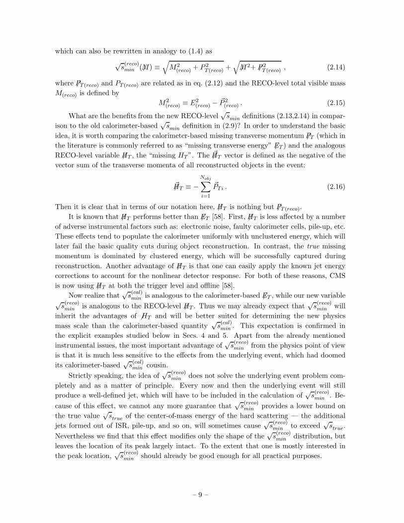
Figure 2: A rearrangement of Fig. 1 into an event topology exhibiting a well defined subsystem

(delineated by the black rectangle) with total invariant mass√s(sub)

. There are nsub visible particles

Xi, i = 1, 2, . . . , nsub, originating from within the subsystem, while the remaining nvis − nsub visible

particles Xnsub+1, . . . , Xnvisare created upstream, outside the subsystem. The subsystem results

from the production and decays of a certain number of parent particles Pj , j = 1, 2, . . . , np, (some

of) which may decay semi-invisibly. All invisible particles χ1, . . . , χninvare then assumed to originate

from within the subsystem.

3. Definition of the subsystem variable√s(sub)min

In this section we propose an alternative modification of the original√smin variable, which

solves the underlying event problem completely and as a matter of principle. The downside

of this approach is that it is not as general and universal as the one discussed in the previous

section, and can be applied only in cases where one can unambiguously identify a subsystem

of the original event topology which is untouched by the underlying event. The basic idea

is schematically illustrated in Fig. 2, which is nothing but a slight rearrangement of Fig. 1

exhibiting a well defined subsystem (delineated by the black rectangle). The original nvis

visible particle Xi from Fig. 1 have now been divided into two groups as follows:

1. There are nsub visible particles X1, . . . ,Xnsuboriginating from within the subsystem.

Their total energy and total momentum are denoted by E(sub) and ~P(sub), correspond-

– 10 –

ingly. The subsystem particles are chosen so that to guarantee that they could not have

come from the underlying event.

2. The remaining nvis − nsub visible particles Xnsub+1, . . . ,Xnvisare created upstream

(outside the subsystem) and have total energy E(up) and total momentum ~P(up). The

upstream particles may originate from the underlying event or from decays of heavier

particles upstream – this distinction is inconsequential at this point.

We also assume that all invisible particles χ1, . . . , χninvoriginate from within the subsystem,

i.e. that no invisible particles are created upstream. In effect, all we have done in Fig. 2 is

to partition the original measured values of the total visible energy E and 3-momentum ~P

from Fig. 1 into two separate components as

E = E(up) + E(sub) , (3.1)

~P = ~P(up) + ~P(sub) . (3.2)

Notice that now the missing transverse momentum is defined as

6~PT ≡ −~PT (up) − ~PT (sub) , (3.3)

while the total visible invariant mass M(sub) of the subsystem is given by

M2(sub) = E2

(sub) − ~P 2(sub) . (3.4)

At this point the reader may be wondering what are the guiding principles for categorizing

a given visible particle Xi as a subsystem or an upstream particle. Since our goal is to identify

a subsystem which is shielded from the effects of the underlying event, the safest way to do

the partition of the visible particles is to require that all QCD jets belong to the upstream

particles, while the subsystem particles consist of objects which are unlikely to come from

the underlying event, such as isolated electrons, photons and muons (and possibly identified

τ -jets and, to a lesser extent, tagged b-jets).

With those preliminaries, we are now ready to ask the usual√smin question: Given

the measured values of E(up), E(sub), ~P(up) and ~P(sub), what is the minimum value√s(sub)min

of the subsystem Mandelstam invariant mass variable√s(sub)

, which is consistent with those

measurements? Proceeding as in [1], once again we find a very simple universal answer,

which, with the help of (3.3) and (3.4), can be equivalently written in several different ways

– 11 –

as follows:

√s(sub)min (6M) =

{

(

√

E2(sub) − P 2

z(sub) +√

6M2+ 6P 2T

)2

− P 2T (up)

}12

(3.5)

=

{

(

√

M2(sub) + P 2

T (sub) +√

6M2+ 6P 2T

)2

− P 2T (up)

}12

(3.6)

=

{

(

√

M2(sub) + P 2

T (sub) +√

6M2+ 6P 2T

)2

− (~PT (sub)+ 6~PT )2

}12

(3.7)

= ||pT (sub)+ 6pT || , (3.8)

where in the last line we have introduced the Lorentz 1+2 vectors

pT (sub) ≡(√

M2(sub)

+ P 2T (sub)

, ~PT (sub)

)

; (3.9)

6pT ≡(

√

6M2+ 6P 2T , 6~PT

)

. (3.10)

As usual, the length of a 1+2 vector is computed as ||p|| = √p · p =

√

p20 − p21 − p22.

Before we proceed to the examples of the next few sections, as a sanity check of the

obtained result it is useful to consider some limiting cases. First, by taking the upstream

visible particles to be an empty set, i.e. ~PT (up) → 0, we recover the usual expression for√smin given in eqs. (1.2,1.4). Next, consider a case with no invisible particles, i.e. 6M = 0

and correspondingly, 6 ~PT = 0. In that case we obtain that√s(sub)min = M(sub), which is of

course the correct result. Finally, suppose that there are no visible subsystem particles, i.e.

E(sub) = ~P(sub) = M(sub) = 0. In that case we obtain√s(sub)min = 6M , which is also the correct

answer.

As we shall see, the subsystem concept of Fig. 2 will be most useful when the subsystem

results from the production and decays of a certain number np of parent particles Pj with

masses MPj, j = 1, 2, . . . , np, correspondingly. Then the total combined mass of all parent

particles is given by

Mp ≡np∑

j=1

MPj. (3.11)

By the conjecture of ref. [1], the location of the peak of the√s(sub)min (6M) distribution will

provide an approximate measurement of Mp as a function of the unknown parameter 6M .

By construction, the obtained relationship Mp(6M) will then be completely insensitive to the

effects from the underlying event.

At this point it may seem that by excluding all QCD jets from the subsystem, we have

significantly narrowed down the number of potential applications of the√s(sub)min variable. Fur-

thermore, we have apparently reintroduced a certain amount of model-dependence which the

original√smin approach was trying so hard to avoid. Those are in principle valid objections,

– 12 –

which can be overcome by using the√s(reco)min variable introduced in the previous section.

Nevertheless, we feel that the√s(sub)min variable can prove to be useful in its own right, and

in a wide variety of contexts. To see this, note that the typical hadron collider signatures of

the most popular new physics models (supersymmetry, extra dimensions, Little Higgs, etc.)

are precisely of the form exhibited in Fig. 2. One typically considers production of colored

particles (squarks, gluinos, KK-quarks, etc.) whose cross-sections dominate. In turn, these

colored particles shed their color charge by emitting jets and decaying to lighter, uncolored

particles in an electroweak sector. The decays of the latter often involve electromagnetic ob-

jects, which could be targeted for selection in the subsystem. The√s(sub)min variable would then

be the perfect tool for studying the mass scales in the electroweak sector (in the context of

supersymmetry, for example, the electroweak sector is composed of the charginos, neutralinos

and sleptons).

Before we move on to some specific examples illustrating these ideas, one last com-

ment is in order. One may wonder whether the√s(sub)min variable should be computed at the

RECO-level or from the calorimeter. Since the subsystem will usually be defined in terms

of reconstructed objects, the more logical option is to calculate√s(sub)min at the RECO-level

and label it as√s(sub,reco)min . However, to streamline our notation, in what follows we shall

always omit the “reco” part of the superscript and will always implicitly assume that√s(sub)min

is computed at RECO-level.

4. SM example: dilepton events from tt production

In this and the next two sections we illustrate the properties of the new variables√s(reco)min

and√s(sub)min with some specific examples. In this section we discuss an example taken from

the Standard Model, which is guaranteed to be available for early studies at the LHC. We

consider dilepton events from tt pair production, where both W ’s decay leptonically. In this

event topology, there are two missing particles (two neutrinos). Therefore, these events very

closely resemble the typical SUSY-like events, in which there are two missing dark matter

particles. In the next two sections, we shall also consider some SUSY examples. In all cases,

we perform detailed event simulation, including the effects from the underlying event and

detector resolution.

4.1 Event simulation details

Events are generated with PYTHIA [59] (using its default model of the underlying event) at

an LHC of 14 TeV, and then reconstructed with the PGS detector simulation package [60].

We have made certain modifications in the publicly available version of PGS to better match

it to the CMS detector. For example, we take the hadronic calorimeter resolution to be [61]

σ

E=

120%√E

, (4.1)

– 13 –

while the electromagnetic calorimeter resolution is [61]

( σ

E

)2=

(

S√E

)2

+

(

N

E

)2

+ C2 , (4.2)

where the energy E is measured in GeV, S = 3.63% is the stochastic term, N = 0.124 is the

noise and C = 0.26% is the constant term. Muons are reconstructed within |η| < 2.4, and we

use the muon global reconstruction efficiency quoted in [61]. We use default pT cuts on the

reconstructed objects as follows: 3 GeV for muons, 10 GeV for electrons and photons, and

15 GeV for jets.

For the tt example presented in this section, we use the approximate next-to-next-to-

leading order tt cross-section of σtt = 894 ± 4+73+12−46−12 pb at a top mass of mt = 175 GeV [62].

For the SUSY examples in the next two sections we use leading order cross-sections.

Since our examples are meant for illustration purposes only, we do not include any

backgrounds to the processes being considered, nor do we require any specific triggers. A

detailed study of the dilepton tt signature including all those effects will appear elsewhere [63].

4.2√s(reco)min variable

We first consider SUSY-like missing energy events arising from tt production, where each

W -boson is forced to decay leptonically (to an electron or a muon). We do not impose any

trigger or offline requirements, and simply plot directly the output from PGS5. We show

various√s quantities of interest in Fig. 3, setting 6M = 0, since in this case the missing

particles are neutrinos and are massless. The dotted (yellow-shaded) histogram represents

the true√s distribution of the tt pair. It quickly rises at the tt mass threshold

Mp ≡ 2mt = 350 GeV (4.3)

and then eventually falls off at large√s due to the parton density function suppression.

Because the top quarks are typically produced with some boost, the√strue distribution in

Fig. 3 peaks a little bit above threshold:(√

strue)

peak> Mp . (4.4)

It is clear that if one could directly measure the√strue distribution, or at least its onset,

the tt mass scale will be easily revealed. Unfortunately, the escaping neutrinos make such a

measurement impossible, unless one is willing to make additional model-dependent assump-

tions6.5Therefore, our plots in this subsection are normalized to a total number of events equal to σtt×BR(W →

e, µ)2.6For example, one can use the known values of the neutrino, W and top masses to solve for the neutrino

kinematics (up to discrete ambiguities). However, this method assumes that the full mass spectrum is already

known, and furthermore, uses the knowledge of the top decay topology to perfectly solve the combinatorics

problem discussed in the Introduction. As an example, consider a case where the lepton is produced first

and the b-quark second, i.e. when the top first decays to a lepton and a leptoquark, which in turn decays to

a neutrino and a b-quark. The kinematic method would then be using the wrong on-shell conditions. The

advantage of the√smin approach is that it is fully inclusive and does not make any reference to the actual

decay topology.

– 14 –

Figure 3: Distributions of various√smin quantities discussed in the text, for the dilepton tt sample

at the LHC with 14 TeV CM energy and 0.5 fb−1 of data. The dotted (yellow-shaded) histogram gives

the true√s distribution of the tt pair. The blue histogram is the distribution of the calorimeter-based√

s(cal)min variable in the ideal case when all effects from the underlying event are turned off. The red

histogram shows the corresponding result for√s(cal)min in the presence of the underlying event. The black

histogram is the distribution of the√s(reco)min variable introduced in Sec. 2. All

√smin distributions

are shown for 6M = 0.

Fig. 3 also shows two versions of the calorimeter-based√s(cal)min variable: the blue (red)

histogram is obtained by switching off (on) the underlying event (ISR and MPI). These

curves reveal two very interesting phenomena. First, without the UE, the peak of the√s(cal)min

distribution (blue histogram) is very close to the parent mass threshold [1]:

no UE =⇒(√

s(cal)min

)

peak≈ Mp . (4.5)

The main observation of Ref. [1] was that this correlation offers an alternative, fully inclusive

and model-independent, method of estimating the mass scale Mp of the parent particles, even

when some of their decay products are invisible and not seen in the detector.

Unfortunately, the “no UE” limit of eq. (4.5) is unphysical, and the corresponding√s(cal)min

distribution (blue histogram in in Fig. 3) is unobservable. What is worse, when one tries to

measure the√s(cal)min distribution in the presence of the UE (red histogram in Fig. 3), the

resulting peak is very far from the physical threshold:

with UE =⇒(√

s(cal)min

)

peak≫ Mp . (4.6)

– 15 –

In the tt example of Fig. 3, the shift is on the order of 1 TeV! It appears therefore that in

practice the√s(cal)min peak would be uncorrelated with any physical mass scale, and instead

would be completely determined by the (uninteresting) physics of the underlying event. Once

the nice model-independent correlation of eq. (4.5) is destroyed by the UE, it becomes of only

academic value [1, 6, 51–53].

However, Fig. 3 also suggests the solution to this difficult problem. If we look at the

distribution of the√s(reco)min variable (black solid histogram), we see that its peak has returned

to the desired value:(√

s(reco)min

)

peak≈ Mp , (4.7)

thus resurrecting the original proposal of Ref. [1]. In order to measure physical mass thresh-

olds, one simply needs to investigate the distribution of the inclusive√s(reco)min variable, which

is calculated at RECO-level. Each peak in that distribution signals the opening of a new

channel, and from (4.7) the location of the peak provides an immediate estimate of the total

mass of all particles involved in the production. Of course, the√s(reco)min distribution is now

not as sharply peaked as the unphysical “no UE” case of√s(cal)min , but as long as its peak is

found in the right location, the method of Ref. [1] becomes viable once again.

Our first main result is therefore nicely summarized in Fig. 3, which shows a total of 4

distributions, 3 of which are either unphysical (the blue histogram of√s(cal)min in the absence of

the UE), unobservable (the yellow-shaded histogram of√strue), or useless (the red histogram

of√s(cal)min in the presence of the UE). The only distribution in Fig. 3 which is physical,

observable and useful at the same time, is the distribution of√s(reco)min (solid black histogram).

Before concluding this subsection, we explain the reason for the improved performance

of the√s(reco)min variable in comparison to the

√s(cal)min version. As already anticipated in Sec. 2,

the basic idea is that energy deposits which are due to hard particles originating from the

hard scattering, tend to be clustered, while the energy deposits due to the UE tend to be

more uniformly spread throughout the detector. In order to see this pictorially, in Figs. 4

and 5 we show a series of calorimeter maps of the combined ECAL+HCAL energy deposits

as a function of the pseudorapidity η and azimuthal angle φ. Since the calorimeter in PGS is

segmented in cells of (∆η,∆φ) = (0.1, 0.1), each calorimeter tower is represented by a square

pixel, which is color-coded according to the amount of energy present in the tower. We have

chosen the color scheme so that larger deposits correspond to darker colors.

Each calorimeter map figure below has four panels. In the upper two panels the calorime-

ter is filled at the parton level directly from PYTHIA. This corresponds to a perfect detector,

where we ignore any smearing effects due to the finite energy resolution. The lower two plots

in each figure show the corresponding results after PGS simulation. Thus by comparing the

plots in the upper row to those in the bottom row, one can see the effect of the detector

resolution. While the finite detector resolution does play some role, we find that it is of no

particular importance for understanding the reason behind the big swings in the√smin peaks

observed in Fig. 3.

Let us instead concentrate on comparing the plots in the left column versus those in

the right column. The left plots show the absolute energy deposit Eα in the α calorimeter

– 16 –

η-4 -3 -2 -1 0 1 2 3 4

φ

0

1

2

3

4

5

6

(G

eV)

cal

E

0

5

10

15

20

25

30

35

40

(parton level)calE

q

qe

e

η-4 -3 -2 -1 0 1 2 3 4

φ

0

1

2

3

4

5

6

(G

eV)

T,ca

lE

0

5

10

15

20

25

30

35

40

(parton level)T,calE

q

qe

e

η-4 -3 -2 -1 0 1 2 3 4

φ

0

1

2

3

4

5

6

(G

eV)

cal

E

0

5

10

15

20

25

30

35

40

(detector level)calE

q

qe

e

η-4 -3 -2 -1 0 1 2 3 4

φ

0

1

2

3

4

5

6

(G

eV)

T,ca

lE

0

5

10

15

20

25

30

35

40

(detector level)T,calE

q

qe

e

Figure 4: PGS calorimeter map of the energy deposits, as a function of pseudorapidity η and

azimuthal angle φ, for a dilepton tt event with only two reconstructed jets. At the parton level, this

particular event has two b-quarks and two electrons. The location of a b-quark (electron, muon) is

marked with the letter “q” (“e”, “µ”). A grey circle delineates (the cone of) a reconstructed jet,

while a green dotted circle denotes a reconstructed lepton. In the upper two plots the calorimeter is

filled at the parton level directly from PYTHIA, while the lower two plots contain results after PGS

simulation. The left plots show absolute energy deposits Eα, while in the right plots the energy in

each tower is shown projected on the transverse plane as Eα cos θα.

tower, while in the right plots this energy is shown projected on the transverse plane as

Eα cos θα. The difference between the left and the right plots is quite striking. The plots

– 17 –

η-4 -3 -2 -1 0 1 2 3 4

φ

0

1

2

3

4

5

6

(G

eV)

cal

E

0

5

10

15

20

25

30

35

40

(parton level)calE

q

q

µ

e

η-4 -3 -2 -1 0 1 2 3 4

φ

0

1

2

3

4

5

6

(G

eV)

T,ca

lE

0

5

10

15

20

25

30

35

40

(parton level)T,calE

q

q

µ

e

η-4 -3 -2 -1 0 1 2 3 4

φ

0

1

2

3

4

5

6

(G

eV)

cal

E

0

5

10

15

20

25

30

35

40

(detector level)calE

q

q

µ

e

η-4 -3 -2 -1 0 1 2 3 4

φ

0

1

2

3

4

5

6

(G

eV)

T,ca

lE

0

5

10

15

20

25

30

35

40

(detector level)T,calE

q

q

µ

e

Figure 5: The same as Fig. 4, but for an event with three additional reconstructed jets.

on the left exhibit lots of energy, which is deposited mostly in the forward calorimeter cells

(at large |η|) [1]. The plots on the right, on the other hand, show only a few clusters of

energy, concentrated mostly in the central part of the detector. Those energy clusters give

rise to the objects (jets, electrons and photons) which are reconstructed from the calorimeter.

Furthermore, each energy cluster can be easily identified with a parton-level particle in the top

decay chain. In order to exhibit this correlation, in Figs. 4 and 5 we use the following notation

for the parton-level particles: a b-quark (electron, muon) is marked with the letter “q” (“e”,

“µ”). A grey circle delineates (the cone of) a reconstructed jet, while a green dotted circle

– 18 –

Event type PYTHIA parton level after PGS simulation√strue

√s(cal)min

√s(cal)min

√s(reco)min

tt event in Fig. 4 427 1110 1179 363

tt event in Fig. 5 638 2596 2761 736

SUSY event in Fig. 12 1954 3539 3509 2085

Table 1: Selected√s quantities (in GeV) for the events shown in Figs. 4, 5 and 12. The second

column shows the true invariant mass√strue of the parent system: top quark pair in case of Figs. 4

and 5, or gluino pair in case of Fig. 12. The third column shows the value of the√s(cal)min variable

(2.9) calculated at the parton level, without any PGS detector simulation, but with the full detector

acceptance cut of |η| < 4.1. The fourth column lists the value of√s(cal)min obtained after PGS detector

simulation, while the last column shows the value of the√s(reco)min variable defined in (2.13).

marks a reconstructed lepton (electron or muon). The lepton isolation requirement implies

that green circles should be void of large energy deposits off-center, and indeed we observe

this to be the case.

In particular, Fig. 4 shows a bare-bone dilepton tt event with just two reconstructed jets

and two reconstructed leptons (which happen to be both electrons). As seen in the figure,

the two jets can be easily traced back to the two b-quarks at the parton level, and there are

no additional reconstructed jets due to the UE activity. Because the event is so clean and

simple, one might expect to obtain a reasonable value for√smin, i.e. close to the tt threshold.

However, this is not the case, if we use the calorimeter-based measurement√s(cal)min . As seen

in Table 1, the measured value of√s(cal)min is very far off — on the order of 1 TeV, even in the

case of a perfect detector. The reason for this discrepancy is now easy to understand from

Fig. 4. Recall that√s(cal)min is defined in terms of the total energy E(cal) in the calorimeter,

which in turn is dominated by the large deposits in the forward region, which came from the

underlying event. More importantly, those contributions are more or less equally spread over

the forward and backward region of the detector, leading to cancellations in the calculation

of the corresponding longitudinal Pz(cal) momentum component. As a result, the first term

in (2.9) becomes completely dominated by the UE contributions [51].

Let us now see how the calculation of√s(reco)min is affected by the UE. Since object recon-

struction is done with the help of minimum transverse cuts (for clustering and object id),

the relevant calorimeter plots are the maps on the right side in Fig. 4. We see that the large

forward energy deposits which were causing the large shift in√s(cal)min are not incorporated

into any reconstructed objects, and thus do not contribute to the√s(reco)min calculation at all.

In effect, the RECO-level prescription for calculating√smin is leaving out precisely the un-

wanted contributions from the UE, while keeping the relevant contributions from the hard

scattering. As seen from Table 1, the calculated value of√s(reco)min for that event is 363 GeV,

which is indeed very close to the tt threshold. It is also smaller than the true√s value of

427 GeV in that event, which is to be expected, since by design√smin ≤ √

s, and this event

does not have any extra ISR jets to spoil this relation.

It is instructive to consider another, more complex tt dilepton event, such as the one

– 19 –

shown in Fig. 5. The corresponding calculated values for√s(cal)min and

√s(reco)min are shown in

the second row of Table 1. As seen in Fig. 5, this event has additional jets and a lot more

UE activity. As a result, the calculated value of√s(cal)min is shifted by almost 2 TeV from

the nominal√strue value. Nevertheless, the RECO-level prescription nicely compensates for

this effect, and the calculated√s(reco)min value is only 736 GeV, which is within 100 GeV of

the nominal√strue = 638 GeV. Notice that in this example we end up with a situation

where√s(reco)min >

√strue. Fig. 3 indicates that this happens quite often — the tail of the√

s(reco)min distribution is more populated than the (yellow-shaded)

√strue distribution. This

should be no cause for concern. First of all, we are only interested in the peak of the√s(reco)min

distribution, and we do not need to make any comparisons between√s(reco)min and

√strue.

Second, any such comparison would be meaningless, since the value of√strue is a priori

unknown, and unobservable.

4.3√s(sub)min variable

Before concluding this section, we shall use the tt example to also illustrate the idea of

the subsystem√s(sub)min variable developed in Sec. 3. Dilepton tt events are a perfect testing

ground for this idea, since the WW subsystem decays leptonically, without any jet activity.

We therefore define the subsystem as the two hard isolated leptons resulting from the decays of

the W -bosons. Correspondingly, we require two reconstructed leptons (electrons or muons)

at the PGS level7, and plot the distribution of the leptonic subsystem√s(sub)min variable in

Fig. 6. As before, the dotted (yellow-shaded) histogram represents the true√s distribution

of the W+W− pair. As expected, it quickly rises at the WW threshold (denoted by the

vertical arrow), then falls off at large√s. Since the

√s(WW )true distribution is unobservable,

the best we can do is to study the corresponding√s(sub)min distribution shown with the solid

black histogram. In this subsystem example, all UE activity is lumped together with the

upstream b-jets from the top quarks decays, and thus has no bearing on the properties of the

leptonic√s(sub)min . In particular, we find that the value of

√s(sub)min is always smaller than the true√

s(WW )true . More importantly, Fig. 6 demonstrates that the peak in the

√s(sub)min distribution is

found precisely at the mass threshold of the particles (in this case the two W bosons) which

initiated the subsystem. Therefore, in analogy to (4.7) we can also write

(√s(sub)min

)

peak≈ M (sub)

p , (4.8)

where M(sub)p is the combined mass of all the parents initiating the subsystem. Fig. 6 shows

that in the tt example just considered, this relation holds to a very high degree of accuracy.

This example should not leave the reader with the impression that hadronic jets are never

allowed to be part of the subsystem. On the contrary — the subsystem may very well include

reconstructed jets as well. The tt case considered here in fact provides a perfect example to

illustrate the idea.

7The selection efficiency for the two leptons is on the order of 60%, which explains the different normalization

of the distributions in Figs. 3 and 6.

– 20 –

Figure 6: The same as Fig. 3, but for the dilepton subsystem in dilepton tt events with two recon-

structed leptons in PGS. The dotted (yellow-shaded) histogram gives the true√s distribution of the

W+W− pair in those events. The black histogram shows the distribution of the (leptonic) subsystem

variable√s(sub)min defined in Sec. 3. In this case, the subsystem is defined by the two isolated leptons,

while all jets are treated as upstream particles. The vertical arrow marks the W+W− mass threshold.

Let us reconsider the tt dilepton sample, and redefine the subsystem so that we now tar-

get the two top quarks as the parents initiating the subsystem. Correspondingly, in addition

to the two leptons, let us allow the subsystem to include two jets, presumably coming from

the two top quark decays. Unfortunately, in doing so, we must face a variant of the partition-

ing8 combinatorial problem discussed in the introduction: as seen in Fig. 7, the typical jet

multiplicity in the events is relatively high, and we must therefore specify the exact procedure

how to select the two jets which would enter the subsystem. We shall consider three different

approaches.

• B-tagging. We can use the fact that the jets from top quark decay are b-jets, while the

jets from ISR are typically light flavor jets. Therefore, by requiring exactly two b-tags,

and including only the two b-tagged jets as part of the subsystem, we can significantly

increase the probability of selecting the correct jets. Of course, ISR will sometimes

also contribute b-tagged jets from gluon splitting, but that happens rather rarely and

the corresponding contribution can be suppressed by a further invariant mass cut on

the two b-jets. The resulting√s(sub)min distribution for the subsystem of 2 leptons and 2

b-tagged jets is shown in Fig. 8 with the black histogram. We see that, as expected,

the distribution peaks at the tt threshold and this time provides a measurement of the

8By construction, the√smin and

√s(sub)min variables never have to face the ordering combinatorial problem.

– 21 –

Figure 7: Unit-normalized distribution of jet multiplicity in dilepton tt events.

top quark mass:(√

s(sub)min

)

peak≈ M (sub)

p = 2mt = 350 GeV . (4.9)

The disadvantage of this method is the loss in statistics: compare the normalization

of the black histogram in Fig. 8 after applying the two b-tags, to the dotted (yellow-

shaded) distribution of the true tt distribution in the selected inclusive dilepton sample

(without b-tags).

• Selection by jet pT . Here one can use the fact that the jets from top decays are on

average harder than the jets from ISR. Correspondingly, by choosing the two highest

pT jets (regardless of b-tagging), one also increases the probability to select the correct

jet pair. The corresponding distribution is shown in Fig. 8 with the blue histogram,

and is also seen to peak at the tt threshold. An important advantage of this method is

that one does not have to pay the price of reduced statistics due to the two additional

b-tags.

• No selection. The most conservative approach would be to apply no selection criteria

on the jets, and include all reconstructed jets in the subsystem. Then the subsystem√s(sub)min variable essentially reverts back to the RECO-level inclusive variable

√s(reco)min

already discussed in the previous subsection. Not surprisingly, we find the peak of its

distribution (red histogram in Fig. 8) near the tt threshold as well.

All three of these examples show that jets can also be usefully incorporated into the

subsystem. The only question is whether one can find a reliable way of preferentially selecting

jets which are more likely to originate from within the intended subsystem, as opposed to

– 22 –

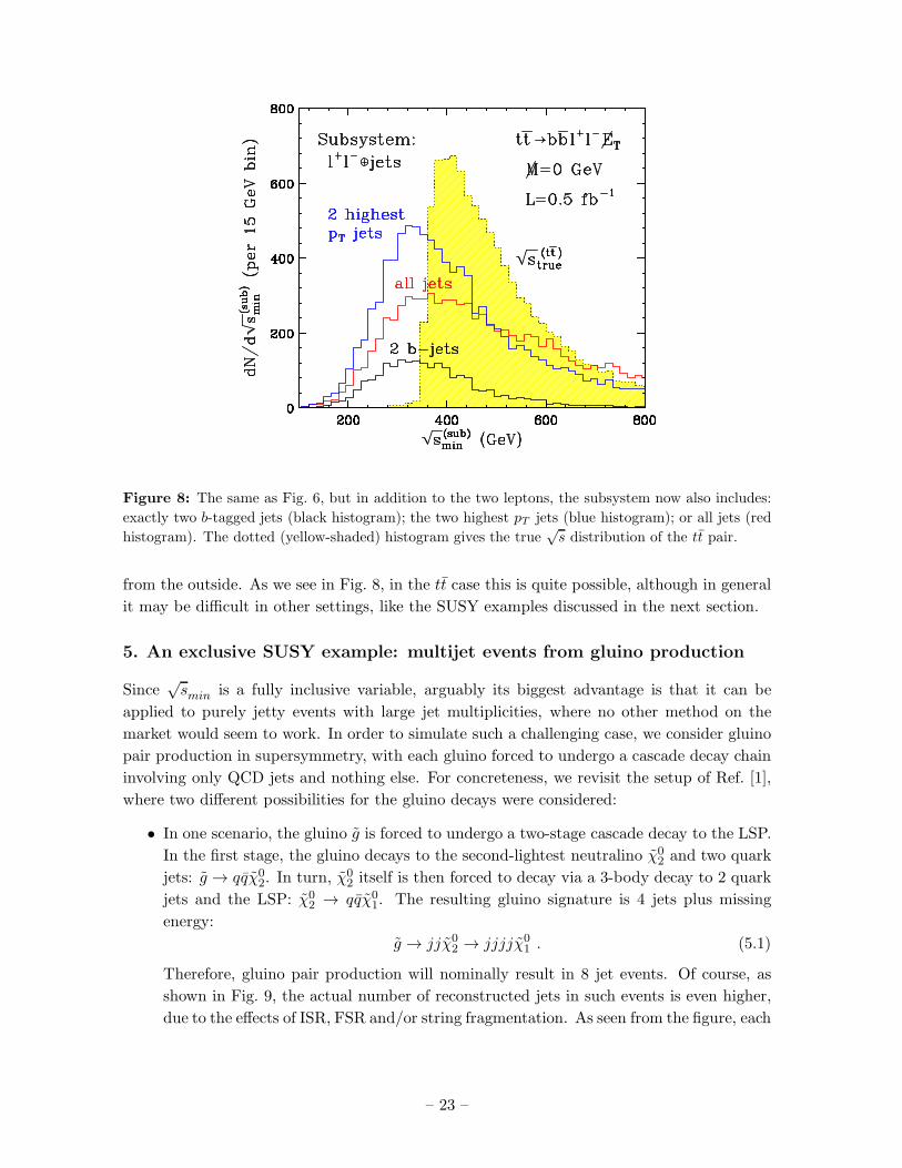
Figure 8: The same as Fig. 6, but in addition to the two leptons, the subsystem now also includes:

exactly two b-tagged jets (black histogram); the two highest pT jets (blue histogram); or all jets (red

histogram). The dotted (yellow-shaded) histogram gives the true√s distribution of the tt pair.

from the outside. As we see in Fig. 8, in the tt case this is quite possible, although in general

it may be difficult in other settings, like the SUSY examples discussed in the next section.

5. An exclusive SUSY example: multijet events from gluino production

Since√smin is a fully inclusive variable, arguably its biggest advantage is that it can be

applied to purely jetty events with large jet multiplicities, where no other method on the

market would seem to work. In order to simulate such a challenging case, we consider gluino

pair production in supersymmetry, with each gluino forced to undergo a cascade decay chain

involving only QCD jets and nothing else. For concreteness, we revisit the setup of Ref. [1],

where two different possibilities for the gluino decays were considered:

• In one scenario, the gluino g is forced to undergo a two-stage cascade decay to the LSP.

In the first stage, the gluino decays to the second-lightest neutralino χ02 and two quark

jets: g → qqχ02. In turn, χ0

2 itself is then forced to decay via a 3-body decay to 2 quark

jets and the LSP: χ02 → qqχ0

1. The resulting gluino signature is 4 jets plus missing

energy:

g → jjχ02 → jjjjχ0

1 . (5.1)

Therefore, gluino pair production will nominally result in 8 jet events. Of course, as

shown in Fig. 9, the actual number of reconstructed jets in such events is even higher,

due to the effects of ISR, FSR and/or string fragmentation. As seen from the figure, each

– 23 –

Figure 9: Unit-normalized distribution of jet multiplicity in gluino pair production events, with each

gluino decaying to four jets and a χ01 LSP as in (5.1).

such event has on average ∼ 10 jets, presenting a formidable combinatorics problem.

We suspect that all9 mass reconstruction methods on the market are doomed if they

were to face such a scenario. It is therefore of particular interest to see how well the√smin method (which is advertized as universally applicable) would fare under such

dire circumstances.

• In the second scenario, the gluino decays directly to the LSP via a three-body decay

g → jjχ01 , (5.2)

so that gluino pair-production events would nominally have 4 jets and missing energy.

For concreteness, in each scenario we fix the mass spectrum as was done in [1]: we use the

approximate gaugino unification relations to relate the gaugino and neutralino masses as

mg = 3mχ02= 6mχ0

1. (5.3)

We can then vary one of these masses, and choose the other two in accord with these relations.

Since we assume three-body decays in (5.2) and (5.1), we do not need to specify the SUSY

scalar mass parameters, which can be taken to be very large. In addition, as implied by

(5.3), we imagine that the lightest two neutralinos are gaugino-like, so that we do not have

to specify the higgsino mass parameter either, and it can be taken to be very large as well.

After these preliminaries, our results for these two scenarios are shown in Figs. 10 and

11, correspondingly. In Fig. 10 (Fig. 11) we consider the 8-jet signature arising from (5.1)

9With the possible exception of the MTgen method of Ref. [32], see Section 7 below.

– 24 –

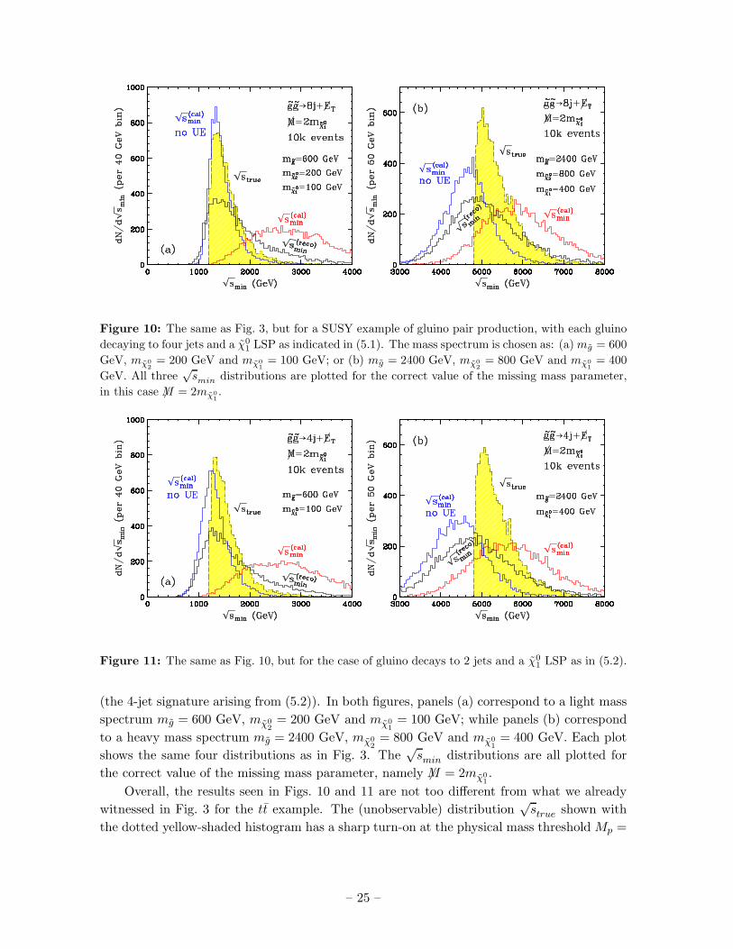
Figure 10: The same as Fig. 3, but for a SUSY example of gluino pair production, with each gluino

decaying to four jets and a χ01 LSP as indicated in (5.1). The mass spectrum is chosen as: (a)mg = 600

GeV, mχ0

2

= 200 GeV and mχ0

1

= 100 GeV; or (b) mg = 2400 GeV, mχ0

2

= 800 GeV and mχ0

1

= 400

GeV. All three√smin distributions are plotted for the correct value of the missing mass parameter,

in this case 6M = 2mχ0

1

.

Figure 11: The same as Fig. 10, but for the case of gluino decays to 2 jets and a χ01 LSP as in (5.2).

(the 4-jet signature arising from (5.2)). In both figures, panels (a) correspond to a light mass

spectrum mg = 600 GeV, mχ02= 200 GeV and mχ0

1= 100 GeV; while panels (b) correspond

to a heavy mass spectrum mg = 2400 GeV, mχ02= 800 GeV and mχ0

1= 400 GeV. Each plot

shows the same four distributions as in Fig. 3. The√smin distributions are all plotted for

the correct value of the missing mass parameter, namely 6M = 2mχ01.

Overall, the results seen in Figs. 10 and 11 are not too different from what we already

witnessed in Fig. 3 for the tt example. The (unobservable) distribution√strue shown with

the dotted yellow-shaded histogram has a sharp turn-on at the physical mass threshold Mp =

– 25 –

η-4 -3 -2 -1 0 1 2 3 4

φ

0

1

2

3

4

5

6

(G

eV)

cal

E

0

5

10

15

20

25

30

35

40

(parton level)calE

q

q

q

q

q

q

q

q

η-4 -3 -2 -1 0 1 2 3 4

φ

0

1

2

3

4

5

6

(G

eV)

T,ca

lE

0

5

10

15

20

25

30

35

40

(parton level)T,calE

q

q

q

q

q

q

q

q

η-4 -3 -2 -1 0 1 2 3 4

φ

0

1

2

3

4

5

6

(G

eV)

cal

E

0

5

10

15

20

25

30

35

40

(detector level)calE

q

q

q

q

q

q

q

q

η-4 -3 -2 -1 0 1 2 3 4

φ

0

1

2

3

4

5

6

(G

eV)

T,ca

lE

0

5

10

15

20

25

30

35

40

(detector level)T,calE

q

q

q

q

q

q

q

q

Figure 12: The same as Fig. 4, but for a SUSY event of gluino pair production, with each gluino

forced to decay to 4 jets and the LSP as in (5.1). The SUSY mass spectrum is as in Figs. 10(a)

and 11(a): mg = 600 GeV, mχ0

2

= 200 GeV and mχ0

1

= 100 GeV. As in Figs. 4 and 5, the circles

denote jets reconstructed in PGS, and here “q” marks the location of a quark from a gluino decay

chain. Therefore, a circle without a “q” inside corresponds to a jet resulting from ISR or FSR, while

a letter “q” without an accompanying circle represents a quark in the gluino decay chain which was

not subsequently reconstructed as a jet.

2mg. If the effects of the UE are ignored, the position of this threshold is given rather well

by the peak of the√s(cal)min distribution (blue histogram). Unfortunately, the UE shifts the

peak in√s(cal)min by 1-2 TeV (red histogram). Fortunately, the distribution of the RECO-level

– 26 –

variable√s(reco)min (black histogram) is stable against UE contamination, and its peak is still

in the right place (near Mp).

Having already seen a similar behavior in the tt example of the previous section, these

results may not seem very impressive, until one realizes just how complicated those events are.

For illustration, Fig. 12 shows the previously discussed calorimeter maps for one particular

“8 jet” event. This event happens to have 11 reconstructed jets, which is consistent with

the typical jet multiplicity seen in Fig. 9. The values of the√s quantities of interest for

this event are listed in Table 1. We see that the RECO prescription for calculating√smin is

able to compensate for a shift in√s of more than 1.5 TeV! A casual look at Fig. 12 should

be enough to convince the reader just how daunting the task of mass reconstruction in such

events is. In this sense, the ease with which the√smin method reveals the gluino mass scale

in Figs. 10 and 11 is quite impressive.

6. An inclusive SUSY example: GMSB study point GM1b

In the Introduction we already mentioned that√smin is a fully inclusive variable. Here we

would like to point out that there are two different aspects of the inclusivity property of√smin:

• Object-wise inclusivity:√smin is inclusive with regards to the type of reconstructed

objects. The definition of√s(reco)min does not distinguish between the different types of

reconstructed objects (and√s(cal)min makes no reference to any reconstructed objects at

all). This makes√smin a very convenient variable to use in those cases where the

newly produced particles have many possible decay modes, and restricting oneself to a

single exclusive signature would cause loss in statistics. For illustration, consider the

gluino pair production example from the previous section. Even though we are always

producing the same type of parent particles (two gluinos), in general they can have

several different decay modes, leading to a very diverse sample of events with varying

number of jets and leptons. Nevertheless, the√s(reco)min distribution, plotted over this

whole signal sample, will still be able to pinpoint the gluino mass scale, as explained in

Sec. 5.

• Event-wise inclusivity:√smin is inclusive also with regards to the type of events, i.e. the

type of new particle production. For simplicity, in our previous examples we have been

considering only one production mechanism at a time, but this is not really necessary —√smin can also be applied in the case of several simultaneous production mechanisms.

In order to illustrate the last point, in this section we shall consider the simultaneous

production of the full spectrum of SUSY particles at a particular benchmark point. We chose

the GM1b CMS study point [64], which is nothing but a minimal gauge-mediated SUSY-

breaking (GMSB) scenario on the SPS8 Snowmass slope [65]. The input parameters are

Λ=80 TeV, Mmes=160 TeV, Nmes=1, tan β = 15 and µ > 0. The physical mass spectrum is

given in Table 2. Point GM1b is characterized by a neutralino NLSP, which promptly decays

– 27 –

uL dL uR dR ℓL νℓ ℓR χ±

2 χ04 χ0

3 g

908 911 872 870 289 278 145 371 371 348 690

t1 b1 t2 b2 τ2 ντ τ1 χ±

1 χ02 χ0

1 G

806 863 895 878 290 277 138 206 206 106 0

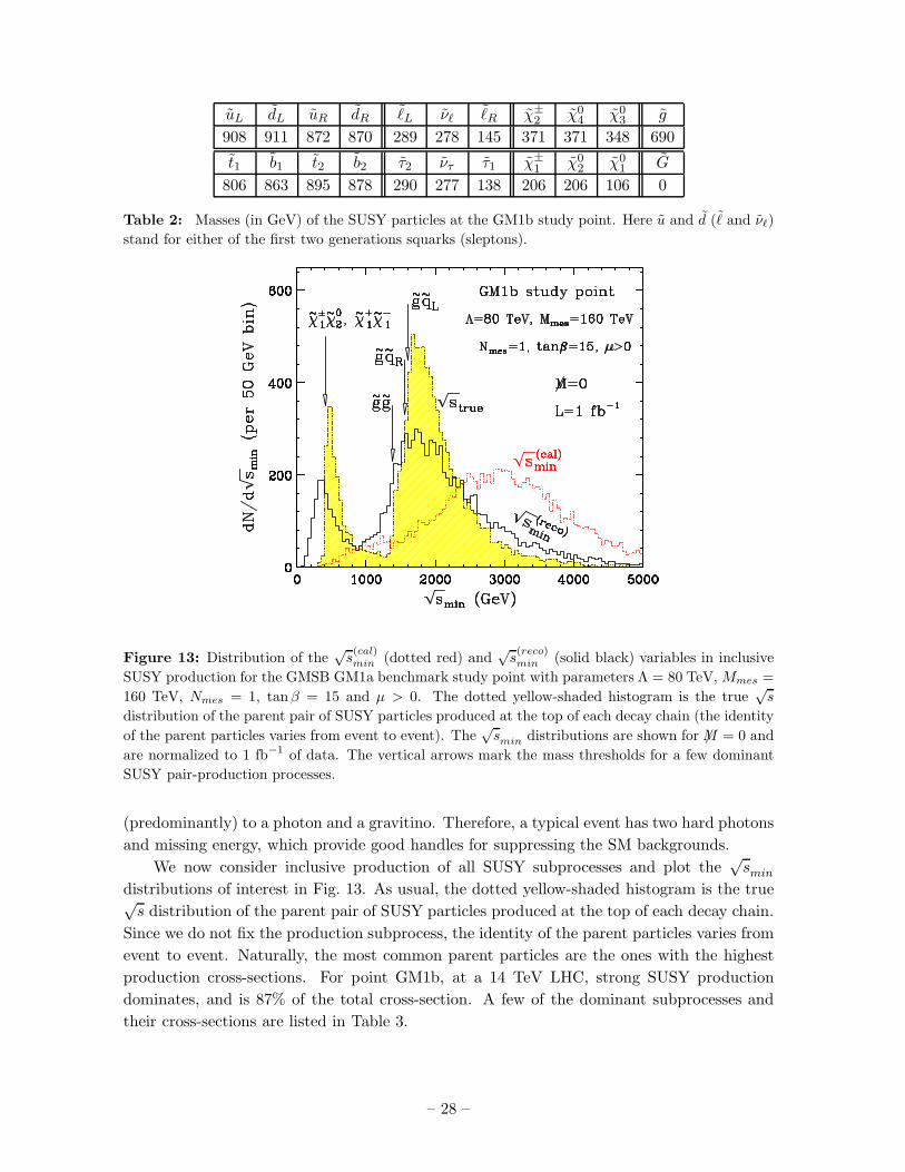
Table 2: Masses (in GeV) of the SUSY particles at the GM1b study point. Here u and d (ℓ and νℓ)

stand for either of the first two generations squarks (sleptons).

Figure 13: Distribution of the√s(cal)min (dotted red) and

√s(reco)min (solid black) variables in inclusive

SUSY production for the GMSB GM1a benchmark study point with parameters Λ = 80 TeV, Mmes =

160 TeV, Nmes = 1, tanβ = 15 and µ > 0. The dotted yellow-shaded histogram is the true√s

distribution of the parent pair of SUSY particles produced at the top of each decay chain (the identity

of the parent particles varies from event to event). The√smin distributions are shown for 6M = 0 and

are normalized to 1 fb−1 of data. The vertical arrows mark the mass thresholds for a few dominant

SUSY pair-production processes.

(predominantly) to a photon and a gravitino. Therefore, a typical event has two hard photons

and missing energy, which provide good handles for suppressing the SM backgrounds.

We now consider inclusive production of all SUSY subprocesses and plot the√smin

distributions of interest in Fig. 13. As usual, the dotted yellow-shaded histogram is the true√s distribution of the parent pair of SUSY particles produced at the top of each decay chain.

Since we do not fix the production subprocess, the identity of the parent particles varies from

event to event. Naturally, the most common parent particles are the ones with the highest

production cross-sections. For point GM1b, at a 14 TeV LHC, strong SUSY production

dominates, and is 87% of the total cross-section. A few of the dominant subprocesses and

their cross-sections are listed in Table 3.

– 28 –

Process χ±

1 χ02 χ+

1 χ−

1 gg gqR gqL qRqR qLqR qLqL

σ (pb) 0.83 0.43 2.03 2.17 1.90 0.36 0.50 0.28

Mp (GeV) 412 412 1380 ∼ 1560 ∼ 1600 ∼ 1740 ∼ 1780 ∼ 1820

Table 3: Cross-sections (in pb) and parent mass thresholds (in GeV) for the dominant production

processes at the GM1b study point. The listed squark cross-sections are summed over the light squark

flavors and conjugate states. The total SUSY cross-section at point GM1b is 9.4 pb.

The true√s distribution in Fig. 13 exhibits an interesting double-peak structure, which

is easy to understand as follows. As we have seen in the exclusive examples from Secs. 4 and 5,

at hadron colliders the particles tend to be produced with√s close to their mass threshold. As

seen in Table 2, the particle spectrum of the GM1b point can be broadly divided (according

to mass) into two groups of superpartners: electroweak sector (the lightest chargino χ±

1 ,

second-to-lightest neutralino χ02 and sleptons) with a mass scale on the order of 200 GeV and

a strong sector (squarks and gluino) with masses of order 700−900 GeV. The first peak in the

true√s distribution (near

√s ∼ 500 GeV) arises from the pair production of two particles

from the electroweak sector, while the second, broader peak in the range of√s ∼ 1500−2300

GeV is due to the pair production of two colored superpartners10. Each one of those peaks

is made up of several contributions from different individual subprocesses, but because their

mass thresholds11 are so close, in the figure they cannot be individually resolved, and appear

as a single bump.

If one could somehow directly observe the true√s SUSY distribution (the dotted yellow-

shaded histogram in Fig. 13), this would lead to some very interesting conclusions. First, from

the presence of two separate peaks one would know immediately that there are two widely

separated scales in the problem. Second, the normalization of each peak would indicate

the relative size of the total inclusive cross-sections (in this example, of the particles in the

electroweak sector versus those in the strong sector). Finally, the broadness of each peak

is indicative of the total number of contributing subprocesses, as well as the typical mass

splittings of the particles within each sector. It may appear surprising that one is able to

draw so many conclusions from a single distribution of an inclusive variable, but this just

comes to show the importance of√s as one of the fundamental collider physics variables.

Unfortunately, because of the missing energy due to the escaping invisible particles, the

true√s distribution cannot be observed, and the best one can do to approximate it is to look

at the distributions of our inclusive√smin variables discussed in Sec. 2: the calorimeter-based√

s(cal)min variable (dotted red histogram in Fig. 13) and the RECO-level

√s(reco)min variable (solid

black histogram in Fig. 13). In the figure, both of those are plotted for 6M = 0.

First let us concentrate on the calorimeter-based version√s(cal)min (dotted red histogram).

We can immediately see the detrimental effects of the UE: first, the electroweak production

peak has been almost completely smeared out, while the strong production peak has been

10The attentive reader may also notice two barely visible bumps (near 950 GeV and 1150 GeV) reflecting

the associated production of one colored and one uncolored particle: gχ±

1 , gχ02 and qχ±

1 , qχ02, correspondingly.

11A few individual mass thresholds are indicated by vertical arrows in Fig. 13.

– 29 –

Figure 14: The same as Fig. 6, but for the GMSB SUSY example considered in Fig. 13. Here the

subsystem is defined in terms of the two hard photons resulting from the two χ01 → G + γ decays.

The vertical arrow marks the onset for inclusive χ01χ

01 production.

shifted upwards by more than a TeV! This behavior is not too surprising, since the same

effect was already encountered in our previous examples in Secs. 4 and 5. Fortunately, we

now also know the solution to this problem: one needs to consider the RECO-level variable√s(reco)min instead, which tracks the true

√s distribution much better. We can see evidence of

this in Fig. 13 as well: notice how the (black)√s(reco)min histogram exhibits the same features

as the (yellow-shaded) true√s distribution. In particular,

√s(reco)min does show two separate

peaks (indicating that SUSY production takes place at two different mass scales), the peaks

are in their proper locations (relative to the missing mass scale 6M), and have the correct

relative width, hinting at the size of the mass splittings in each sector. We thus conclude that

all of the interesting physics conclusions that one would be able to reach from looking at the

true√s distributions, can still be made based on the inclusive distribution of our RECO-level√

s(reco)min variable.

Before concluding this section, we shall take the opportunity to use the GM1b example

to also illustrate the√s(sub)min variable proposed in Sec. 3. As already mentioned, the GM1b

study point corresponds to a GMSB scenario with a promptly decaying Bino-like χ01 NLSP.

Most events therefore contain two hard photons from the two χ01 decays to gravitinos. Then

it is quite natural to define the exclusive subsystem in Fig. 2 in terms of these two photons.

The corresponding√s(sub)min distribution is shown in Fig. 14 with the black solid histogram.

For completeness, in the figure we also show the true√s distribution of the χ0

1 pair (dotted

yellow-shaded histogram). The vertical arrow marks the location of the χ01χ

01 mass threshold.

– 30 –

We notice that the peak of the√s(sub)min distribution nicely reveals the location of the neutralino

mass threshold, and from there the neutralino mass itself. We see that the method of√s(sub)min

provides a very simple way of measuring the NLSP mass in such GMSB scenarios (for an

alternative approach based on MT2, see [66]).

7. Comparison to other inclusive collider variables

Having discussed the newly proposed variables√s(reco)min and

√s(sub)min in various settings in

Secs. 4-6, we shall now compare them to some other global inclusive variables which have

been discussed in the literature in relation to determining a mass scale of the new physics. For

simplicity here we shall concentrate only on the most model-independent variables, which do

not suffer from the topological and combinatorial ambiguities mentioned in the Introduction.

At the moment, there are only a handful of such variables. Depending on the treatment

of the unknown masses of the invisible particles, they can be classified into one of the following

two categories:

• Variables which do not depend on an unknown invisible mass parameter. The most

popular members of this class are the “missing HT ” variable

6HT ≡

∣

∣

∣

∣

∣

∣

−Nobj∑

i=1

~PT i

∣

∣

∣

∣

∣

∣

, (7.1)

which is simply the magnitude of the 6 ~HT vector from eq. (2.16), and the scalar HT

variable

HT ≡ 6HT +

Nobj∑

i=1

PT i . (7.2)

Here we follow the notation from Sec. 2, where ~PT i is the measured transverse mo-

mentum of the i-th reconstructed object in the event (i = 1, 2, . . . , Nobj). The main

advantage of 6HT and HT is their simplicity: both are very general, and are defined

purely in terms of observed quantities, without any unknown mass parameters. The

downside of 6HT and HT is that they cannot be directly correlated with any physical

mass scale in a model-independent way12.

• Variables which exhibit dependence on one or more invisible mass parameters. As two

representatives from this class we shall consider MTgen from Ref. [32] and√s(reco)min from

Sec. 2 here. We shall not repeat the technical definition of MTgen, and instead refer the

uninitiated reader to the original paper [32]. Suffice it to say that the method of MTgen

starts out by assuming exactly two decay chains in each event. The arising combinato-

rial problem is then solved by brute force — by considering all possible partitions of the

12Some early studies of HT -like variables found interesting linear correlations between the peak in the HT

distribution and a suitably defined SUSY mass scale in the context of specific SUSY models, e.g. minimal

supergravity (MSUGRA) [10,67,68], minimal GMSB [67], or mixed moduli-mediation [69]. However, any such

correlations do not survive further scrutiny in more generic SUSY scenarios, see e.g. [70].

– 31 –

event into two sides, computing MT2 for each such partition, and taking the minimum

value of MT2 found in the process. Both MTgen and√s(reco)min introduce a priori unknown

parameters related to the mass scale of the missing particles produced in the event. In

the case of√s(reco)min , this is simply the single parameter 6M , measuring the total invisible

mass (in the sense of a scalar sum as defined in eq. (1.3)). The MTgen variable, on the

other hand, must in principle introduce two separate missing mass parameters 6M1 and

6M2 (one for each side of the event). However, the existing applications of MTgen in

the literature have typically made the assumption that 6M1 = 6M2, although this is not

really necessary and one could just as easily work in terms of two separate inputs 6M1

and 6M2 [3, 4]. The inconvenience of having to deal with unknown mass parameters in

the case of MTgen and√s(reco)min is greatly compensated by the luxury of being able to

relate certain features of their distributions to a fundamental physical mass scale in a

robust, model-independent way. In particular, the upper endpoint M(max)Tgen of the MTgen

distribution gives the larger of the two parent masses max{MP1 ,MP2} [71]. Therefore,

if the two parent masses are the same, i.e. MP1 = MP2 , then the parent mass threshold

Mp = MP1 +MP2 is simply given by

Mp = 2M(max)Tgen . (7.3)

On the other hand, as we have already seen in Secs. 4-6, the peak of the√s(reco)min is

similarly correlated with the parent mass threshold, see eq. (4.7).

In principle, all four13 of these variables are inclusive both object-wise and event-wise. It is

therefore of interest to compare them with respect to:

1. The degree of correlation with the new physics mass scale Mp.

2. Stability of this correlation against the detrimental effects of the UE.

Figs. 15, 16 and 17 allow for such comparisons.

In Fig. 15 we first revisit the case of the dilepton tt sample discussed in Sec. 4. In addition

to the true√s (yellow shaded) and

√s(reco)min (black) distribution already appearing in Fig. 3,

we now also plot the distributions of 2MTgen (red dots), HT (green dots) and 6HT (blue dots),

all calculated at the RECO-level. For completeness, in Fig. 15 we also show a variant of

MTgen, called MTTgen (magenta dots), where all visible particle momenta are first projected

on the transverse plane, before computing MTgen in the usual way [32]14. All results include

the full simulation of the underlying event. For plotting convenience, the 6HT distribution is

shown scaled down by a factor of 2.

13We caution the reader that HT is often defined in a more narrow sense than eq. (7.2). For example,

sometimes the 6HT term is omitted, sometimes the sum in eq. (7.2) is limited to the reconstructed jets only;

or to the four highest pT jets only; or to all jets, but starting from the second-highest pT one.14We caution the reader that the definition of MTTgen cannot be found in the published version of Ref. [32]

— the MTTgen discussion was added in a recent replacement on the archive, which appeared more than two

years after the original publication.

– 32 –

Figure 15: The same as Fig. 3, but now in addition to the true√s (yellow shaded) and

√s(reco)min

(black) distribution, we also plot the distributions of 2MTgen (red dots), 2MTTgen (magenta dots),

HT (green dots) and 6HT (blue dots), all calculated at the RECO-level. All results include the full

simulation of the underlying event. For plotting convenience, the 6HT distribution is shown scaled

down by a factor of 2. The vertical dotted line marks the tt mass threshold Mp = 2mt = 350 GeV.

Based on the results from Fig. 15, we can now address the question, which inclusive

distribution shows the best correlation with the parent mass scale (in this case the parent

mass scale is the tt mass threshold Mp = 2mt = 350 GeV marked by the vertical dotted

line in Fig. 15). Let us begin with the two variables, 6HT and HT , which do not depend

on any unknown mass parameters. Fig. 15 reveals that the 6HT distribution peaks very far

from threshold, and therefore does not reveal much information about the new physics mass

scale. Consequently, any attempt at extracting new physics parameters out of the missing

energy distribution alone, must make some additional model-dependent assumptions [72]. On

the other hand, the HT distribution appears to correlate better with Mp, since its peak is

relatively close to the tt threshold. However, this relationship is purely empirical, and it is

difficult to know what is the associated systematic error.

Moving on to the variables which carry a dependence on a missing mass parameter,√s(reco)min , 2MTgen and 2MTTgen, we see that all three are affected to some extent by the

presence of the UE. In particular, the distributions of 2MTgen and 2MTTgen are now smeared

and extend significantly beyond their expected endpoint (7.3). Not surprisingly, the UE has

a larger impact on 2MTgen than on 2MTTgen. In either case, there is no obvious endpoint.

Nevertheless, one could in principle try to extract an endpoint through a straight-line fit, for

example, but it is clear that the obtained value will be wrong by a certain amount (depending

– 33 –

Figure 16: The same as Fig. 15, but for the gluino pair production example from Sec. 5, with each

gluino decaying to 4 jets as in (5.1). We use the light SUSY mass spectrum from Fig. 10(a). The

vertical dotted line now shows the gg mass threshold Mp = 2mg = 1200 GeV.

on the chosen region for fitting and on the associated backgrounds). All these difficulties with

2MTgen and 2MTTgen are simply a reflection of the challenge of measuring a mass scale from

an endpoint as in (7.3), instead of from a peak as in (4.7). By comparison, the determination

of the new physics mass scale from the√s(reco)min distribution is much more robust. As shown

in Fig. 15, the√s(reco)min peak is barely affected by the UE, and is still found precisely in the

right location.

All of the above discussion can be directly applied to the SUSY examples considered in

Sec. 5 as well. As an illustration, Figs. 16 and 17 revisit two of the gluino examples from

Section 5. In both figures, we consider gluino pair-production with a light SUSY spectrum

(mχ01= 100 GeV, mχ0

2= 200 GeV and mg = 600 GeV). Then in Fig. 16 each gluino decays

to 4 jets as in eq. (5.1), while in Fig. 17 each gluino decays to 2 jets as in eq. (5.2). (Thus

Fig. 16 is the analogue of Fig. 10(a), while Fig. 17 is the analogue of Fig. 11(a).)

The conclusions from Figs. 16 and 17 are very similar. Both figures confirm that 6HT

is not very helpful in determining the gluino mass scale Mp = 2mg = 1200 GeV (indicated

by the vertical dotted line). The HT distribution, on the other hand, has a nice well-defined

peak, but the location of the HT peak always underestimates the gluino mass scale (by about

250 GeV in each case). Figs. 16 and 17 also confirm the effect already seen in Fig. 15: that the

underlying event causes the 2MTgen and 2MTTgen distributions to extend well beyond their

upper kinematic endpoint, thus violating (7.3) and making the corresponding extraction of

Mp rather problematic. In fact, just by looking at Figs. 16 and 17, one might be tempted to

– 34 –

Figure 17: The same as Fig. 16, but with each gluino decaying to 2 jets as in (5.2). Compare to

Fig. 11(a).

deduce that, if anything, it is the peak in 2MTgen that perhaps might indicate the value of the

new physics mass scale and not the 2MTgen endpoint. Finally, the√s(reco)min distribution also

feels to some extent the effects from the UE, but always has its peak in the near vicinity of

Mp. Therefore, among the five inclusive variables under consideration here,√s(reco)min appears

to provide the best estimate of the new physics mass scale. The correlation (4.7) advertized

in this paper is seen to hold very well in Fig. 17 and reasonably well in Fig. 16.

8. Summary and conclusions

Since the original proposal of the√smin variable in Ref. [1], its practicability has been called

into question in light of the effects from the underlying event, in particular initial state

radiation and multiple parton interactions. In this paper we proposed two variations of the√smin variable which are intended to avoid this problems.

1. RECO-level√s(reco)min . The first variant, the RECO-level variable

√s(reco)min introduced

in Sec. 2, is basically a modification of the prescription for computing the original√smin variable: instead of using (muon-corrected) calorimeter deposits, as was done

in [1, 51], one could instead calculate√smin with the help of the reconstructed objects

(jets and isolated photons, electrons and muons). Our examples in Sections 4, 5 and

6 showed that this procedure tends to automatically subtract out the bulk of the UE

contributions, rendering the√s(reco)min variable safe.

– 35 –

2. Subsystem√s(sub)min . Our second suggestion, discussed in Sec. 3, was to apply

√smin to

a subsystem of the observed event, which is suitably defined so that it does not include

the contributions from the underlying event. The easiest way to do this is to veto jets

from entering the definition of the subsystem. In this case, the subsystem variable√s(sub)min is completely unaffected by the underlying event. However, depending on the

particular scenario, in principle one could also allow (certain kinds of) jets to enter the

subsystem. As long as there is an efficient method (through cuts) of selecting jets which

(most likely) did not originate from the UE, this should work as well, as demonstrated

in Fig. 6 with our tt example.

Being simply variants of the original√smin variable, both

√s(reco)min and

√s(sub)min auto-

matically inherit the many nice properties of√smin:

• Both√s(reco)min and

√s(sub)min have a clear physical meaning: the minimum CM energy

in the (sub)system, which is required in order to explain the observed signal in the

detector.

• Both√s(reco)min and

√s(sub)min are defined in a manifestly 1+3 Lorentz invariant way. As

a consequence, their definitions utilize the available information about the longitudinal

momentum components of the particles observed in the detector.

• Both√s(reco)min and

√s(sub)min can be computed by simple analytical formulas, eqs. (2.13,2.14)

and (3.5-3.8), correspondingly.

• √s(reco)min (and to some extent

√s(sub)min ) is a general, global, and inclusive variable, which

can be applied to any type of events, regardless of the event topology, number or type

of reconstructed objects, number or type of missing particles, etc. For example, all of

the arbitrariness associated with the number and type of missing particles is encoded

by a single parameter 6M .

• The most important property of both√s(reco)min and

√s(sub)min is that they exhibit a peak

in their distributions, which directly correlates with the mass scale Mp of the parent

particles. In this regard we remind the reader that, compared to a kinematic endpoint,

a peak is a feature which is much easier to observe and subsequently measure precisely

over the SM backgrounds. This point was specifically illustrated in Sec. 7, where we

contrasted the observability of the peak in the√s(reco)min distribution to the observability

of the endpoints of the 2MTgen and 2MTTgen distributions.

At the same time, compared to the original calorimeter-based√smin variable considered

in Ref. [1], the new variables√s(reco)min and

√s(sub)min proposed here have one crucial advantage:

they have very little sensitivity to the effects from the underlying event (ISR and MPI). As

a result, the measurement of the corresponding mass scale from the peak in the distribution

of√s(reco)min or

√s(sub)min is robust and physically meaningful.

In conclusion, we have shown that the variables√s(reco)min and

√s(sub)min have certain im-

portant advantages, and we feel that the experimental collaborations at the Tevatron and

the LHC can only benefit from including them among their arsenal of observables.

– 36 –

Acknowledgments

We thank A. Barr, C. Lester, F. Moortgat, L. Pape and B. Webber for stimulating discussions

and correspondence. This work is supported in part by a US Department of Energy grant

DE-FG02-97ER41029. SLAC is operated by Stanford University for the US Department of

Energy under contract DE-AC02-76SF00515.

References

[1] P. Konar, K. Kong and K. T. Matchev, “√smin : A Global inclusive variable for determining

the mass scale of new physics in events with missing energy at hadron colliders,” JHEP 0903,

085 (2009) [arXiv:0812.1042 [hep-ph]].

[2] S. Chang and A. de Gouvea, “Neutrino Alternatives For Missing Energy Events At Colliders,”

Phys. Rev. D 80, 015008 (2009) [arXiv:0901.4796 [hep-ph]].

[3] A. J. Barr, B. Gripaios and C. G. Lester, “Transverse masses and kinematic constraints: from

the boundary to the crease,” JHEP 0911, 096 (2009) [arXiv:0908.3779 [hep-ph]].

[4] P. Konar, K. Kong, K. T. Matchev and M. Park, “Dark Matter Particle Spectroscopy at the

LHC: Generalizing MT2 to Asymmetric Event Topologies,” JHEP 1004, 086 (2010)

[arXiv:0911.4126 [hep-ph]].

[5] K. Agashe, D. Kim, M. Toharia and D. G. E. Walker, “Distinguishing Dark Matter

Stabilization Symmetries Using Multiple Kinematic Edges and Cusps,” arXiv:1003.0899

[hep-ph].

[6] A. J. Barr and C. G. Lester, “A Review of the Mass Measurement Techniques proposed for the

Large Hadron Collider,” arXiv:1004.2732 [hep-ph].

[7] M. R. Buckley, H. Murayama, W. Klemm and V. Rentala, “Discriminating spin through

quantum interference,” Phys. Rev. D 78, 014028 (2008) [arXiv:0711.0364 [hep-ph]].

[8] M. Burns, K. Kong, K. T. Matchev and M. Park, “A General Method for Model-Independent

Measurements of Particle Spins, Couplings and Mixing Angles in Cascade Decays with Missing

Energy at Hadron Colliders,” JHEP 0810, 081 (2008) [arXiv:0808.2472 [hep-ph]].

[9] F. Boudjema and R. K. Singh, “A model independent spin analysis of fundamental particles

using azimuthal asymmetries,” JHEP 0907, 028 (2009) [arXiv:0903.4705 [hep-ph]].

[10] I. Hinchliffe, F. E. Paige, M. D. Shapiro, J. Soderqvist and W. Yao, “Precision SUSY

measurements at LHC,” Phys. Rev. D 55, 5520 (1997) [arXiv:hep-ph/9610544].

[11] H. Bachacou, I. Hinchliffe and F. E. Paige, “Measurements of masses in SUGRA models at

LHC,” Phys. Rev. D 62, 015009 (2000) [arXiv:hep-ph/9907518].

[12] I. Hinchliffe and F. E. Paige, “Measurements in SUGRA models with large tan(beta) at LHC,”

Phys. Rev. D 61, 095011 (2000) [arXiv:hep-ph/9907519].

[13] B. C. Allanach, C. G. Lester, M. A. Parker and B. R. Webber, “Measuring sparticle masses in

non-universal string inspired models at the LHC,” JHEP 0009, 004 (2000)

[arXiv:hep-ph/0007009].

[14] B. K. Gjelsten, D. J. Miller and P. Osland, “Measurement of SUSY masses via cascade decays

for SPS 1a,” JHEP 0412, 003 (2004) [arXiv:hep-ph/0410303].

– 37 –

[15] B. K. Gjelsten, D. J. Miller and P. Osland, “Measurement of the gluino mass via cascade

decays for SPS 1a,” JHEP 0506, 015 (2005) [arXiv:hep-ph/0501033].

[16] A. Birkedal, R. C. Group and K. Matchev, “Slepton mass measurements at the LHC,” In the

Proceedings of 2005 International Linear Collider Workshop (LCWS 2005), Stanford,

California, 18-22 Mar 2005, pp 0210 [arXiv:hep-ph/0507002].

[17] D. J. Miller, P. Osland and A. R. Raklev, “Invariant mass distributions in cascade decays,”

JHEP 0603, 034 (2006) [arXiv:hep-ph/0510356].

[18] D. Costanzo and D. R. Tovey, “Supersymmetric particle mass measurement with invariant

mass correlations,” JHEP 0904, 084 (2009) [arXiv:0902.2331 [hep-ph]].

[19] M. Burns, K. T. Matchev and M. Park, “Using kinematic boundary lines for particle mass

measurements and disambiguation in SUSY-like events with missing energy,” JHEP 0905, 094

(2009) [arXiv:0903.4371 [hep-ph]].

[20] K. T. Matchev, F. Moortgat, L. Pape and M. Park, “Precise reconstruction of sparticle masses

without ambiguities,” JHEP 0908, 104 (2009) [arXiv:0906.2417 [hep-ph]].

[21] M. Burns, K. Kong, K. T. Matchev and M. Park, “Using Subsystem MT2 for Complete Mass

Determinations in Decay Chains with Missing Energy at Hadron Colliders,” JHEP 0903, 143

(2009) [arXiv:0810.5576 [hep-ph]].

[22] M. M. Nojiri, G. Polesello and D. R. Tovey, “Proposal for a new reconstruction technique for

SUSY processes at the LHC,” arXiv:hep-ph/0312317.

[23] K. Kawagoe, M. M. Nojiri and G. Polesello, “A new SUSY mass reconstruction method at the

CERN LHC,” Phys. Rev. D 71, 035008 (2005) [arXiv:hep-ph/0410160].

[24] H. C. Cheng, J. F. Gunion, Z. Han, G. Marandella and B. McElrath, “Mass Determination in

SUSY-like Events with Missing Energy,” JHEP 0712, 076 (2007) [arXiv:0707.0030 [hep-ph]].

[25] M. M. Nojiri, G. Polesello and D. R. Tovey, “A hybrid method for determining SUSY particle

masses at the LHC with fully identified cascade decays,” JHEP 0805, 014 (2008)

[arXiv:0712.2718 [hep-ph]].

[26] H. C. Cheng, D. Engelhardt, J. F. Gunion, Z. Han and B. McElrath, “Accurate Mass

Determinations in Decay Chains with Missing Energy,” Phys. Rev. Lett. 100, 252001 (2008)

[arXiv:0802.4290 [hep-ph]].

[27] H. C. Cheng, J. F. Gunion, Z. Han and B. McElrath, “Accurate Mass Determinations in Decay

Chains with Missing Energy: II,” Phys. Rev. D 80, 035020 (2009) [arXiv:0905.1344 [hep-ph]].

[28] B. Webber, “Mass determination in sequential particle decay chains,” JHEP 0909, 124 (2009)

[arXiv:0907.5307 [hep-ph]].

[29] M. M. Nojiri, K. Sakurai and B. R. Webber, “Reconstructing particle masses from pairs of

decay chains,” arXiv:1005.2532 [hep-ph].

[30] C. G. Lester and D. J. Summers, “Measuring masses of semi-invisibly decaying particles pair

produced at hadron colliders,” Phys. Lett. B 463, 99 (1999) [arXiv:hep-ph/9906349].

[31] A. Barr, C. Lester and P. Stephens, “m(T2): The truth behind the glamour,” J. Phys. G 29,

2343 (2003) [arXiv:hep-ph/0304226].

– 38 –

[32] C. Lester and A. Barr, “MTGEN : Mass scale measurements in pair-production at colliders,”

JHEP 0712, 102 (2007) [arXiv:0708.1028 [hep-ph]].

[33] W. S. Cho, K. Choi, Y. G. Kim and C. B. Park, “Gluino Stransverse Mass,” Phys. Rev. Lett.

100, 171801 (2008) [arXiv:0709.0288 [hep-ph]].

[34] B. Gripaios, “Transverse Observables and Mass Determination at Hadron Colliders,” JHEP

0802, 053 (2008) [arXiv:0709.2740 [hep-ph]].

[35] A. J. Barr, B. Gripaios and C. G. Lester, “Weighing Wimps with Kinks at Colliders: Invisible

Particle Mass Measurements from Endpoints,” JHEP 0802, 014 (2008) [arXiv:0711.4008

[hep-ph]].

[36] W. S. Cho, K. Choi, Y. G. Kim and C. B. Park, “Measuring superparticle masses at hadron

collider using the transverse mass kink,” JHEP 0802, 035 (2008) [arXiv:0711.4526 [hep-ph]].

[37] H. C. Cheng and Z. Han, “Minimal Kinematic Constraints and MT2,” JHEP 0812, 063 (2008)

[arXiv:0810.5178 [hep-ph]].

[38] K. T. Matchev, F. Moortgat, L. Pape and M. Park, “Precision sparticle spectroscopy in the

inclusive same-sign dilepton channel at LHC,” arXiv:0909.4300 [hep-ph].

[39] P. Konar, K. Kong, K. T. Matchev and M. Park, “Superpartner mass measurements with 1D

decomposed MT2,” arXiv:0910.3679 [hep-ph].

[40] D. R. Tovey, “On measuring the masses of pair-produced semi-invisibly decaying particles at

hadron colliders,” JHEP 0804, 034 (2008) [arXiv:0802.2879 [hep-ph]].

[41] G. Polesello and D. R. Tovey, “Supersymmetric particle mass measurement with the

boost-corrected contransverse mass,” JHEP 1003, 030 (2010) [arXiv:0910.0174 [hep-ph]].

[42] K. T. Matchev and M. Park, “A general method for determining the masses of semi-invisibly

decaying particles at hadron colliders,” arXiv:0910.1584 [hep-ph].

[43] T. Han, I. W. Kim and J. Song, “Kinematic Cusps: Determining the Missing Particle Mass at

the LHC,” arXiv:0906.5009 [hep-ph].

[44] A. Alves, O. Eboli and T. Plehn, “It’s a gluino,” Phys. Rev. D 74, 095010 (2006)

[arXiv:hep-ph/0605067].

[45] J. M. Butterworth, J. R. Ellis and A. R. Raklev, “Reconstructing sparticle mass spectra using

hadronic decays,” JHEP 0705, 033 (2007) [arXiv:hep-ph/0702150].

[46] C. Csaki, J. Heinonen and M. Perelstein, “Testing Gluino Spin with Three-Body Decays,”

JHEP 0710, 107 (2007) [arXiv:0707.0014 [hep-ph]].

[47] M. M. Nojiri, K. Sakurai, Y. Shimizu and M. Takeuchi, “Handling jets + missing ET channel

using inclusive mT2,” JHEP 0810, 100 (2008) [arXiv:0808.1094 [hep-ph]].

[48] M. M. Nojiri, Y. Shimizu, S. Okada and K. Kawagoe, “Inclusive transverse mass analysis for

squark and gluino mass determination,” JHEP 0806, 035 (2008) [arXiv:0802.2412 [hep-ph]].

[49] J. Alwall, K. Hiramatsu, M. M. Nojiri and Y. Shimizu, “Novel reconstruction technique for

New Physics processes with initial state radiation,” Phys. Rev. Lett. 103, 151802 (2009)

[arXiv:0905.1201 [hep-ph]].

[50] M. M. Nojiri and M. Takeuchi, “Study of the top reconstruction in top-partner events at the

LHC,” JHEP 0810, 025 (2008) [arXiv:0802.4142 [hep-ph]].

– 39 –

[51] A. Papaefstathiou and B. Webber, “Effects of QCD radiation on inclusive variables for

determining the scale of new physics at hadron colliders,” JHEP 0906, 069 (2009)

[arXiv:0903.2013 [hep-ph]].

[52] A. Papaefstathiou and B. Webber, “Effects of invisible particle emission on inclusive variables

for determining the scale of new physics at hadron colliders,” arXiv:1004.4762 [hep-ph].

[53] G. Brooijmans et al., “New Physics at the LHC. A Les Houches Report: Physics at TeV

Colliders 2009 - New Physics Working Group,” arXiv:1005.1229 [hep-ph].

[54] T. Hur, H. S. Lee and S. Nasri, “A Supersymmetric U(1)’ Model with Multiple Dark Matters,”

Phys. Rev. D 77, 015008 (2008) [arXiv:0710.2653 [hep-ph]].

[55] Q. H. Cao, E. Ma, J. Wudka and C. P. Yuan, “Multipartite Dark Matter,” arXiv:0711.3881

[hep-ph].

[56] H. Sung Cheon, S. K. Kang and C. S. Kim, “Doubly Coexisting Dark Matter Candidates in an

Extended Seesaw Model,” Phys. Lett. B 675, 203 (2009) [arXiv:0807.0981 [hep-ph]].

[57] T. Hur, H. S. Lee and C. Luhn, “Common gauge origin of discrete symmetries in observable

sector and hidden sector,” JHEP 0901, 081 (2009) [arXiv:0811.0812 [hep-ph]].

[58] Greg Landsberg, “ 6ET in CMS”, talk given at the “Missing Energy” workshop, UC Davis, April

1, 2009.

[59] T. Sjostrand, S. Mrenna and P. Skands, “PYTHIA 6.4 physics and manual,” JHEP 0605, 026

(2006) [arXiv:hep-ph/0603175].

[60] J. Conway, “PGS: Simple simulation package for generic collider detectors,”

http://www.physics.ucdavis.edu/∼conway/research/software/pgs/pgs.html.

[61] G. L. Bayatian et al. [CMS Collaboration], “CMS physics: Technical design report,” vol. I:

“Detector Performance and Software”, CERN/LHCC 2006-001.

[62] N. Kidonakis and R. Vogt, “The Theoretical top quark cross section at the Tevatron and the

LHC,” Phys. Rev. D 78, 074005 (2008) [arXiv:0805.3844 [hep-ph]].

[63] P. Konar, K. Kong, K. T. Matchev, and M. Park, in preparation.

[64] https://twiki.cern.ch/twiki/bin/view/Main/SezenSekmen

[65] B. C. Allanach et al., “The Snowmass points and slopes: Benchmarks for SUSY searches,” in

Proc. of the APS/DPF/DPB Summer Study on the Future of Particle Physics (Snowmass

2001) ed. N. Graf, Eur. Phys. J. C 25, 113 (2002) [arXiv:hep-ph/0202233].

[66] K. Hamaguchi, E. Nakamura and S. Shirai, “A Measurement of Neutralino Mass at the LHC

in Light Gravitino Scenarios,” Phys. Lett. B 666, 57 (2008) [arXiv:0805.2502 [hep-ph]].

[67] D. R. Tovey, “Measuring the SUSY mass scale at the LHC,” Phys. Lett. B 498, 1 (2001)

[arXiv:hep-ph/0006276].

[68] J. Hisano, K. Kawagoe and M. M. Nojiri, “A detailed study of the gluino decay into the third

generation squarks at the CERN LHC,” Phys. Rev. D 68, 035007 (2003)

[arXiv:hep-ph/0304214].

[69] R. Kitano and Y. Nomura, “Supersymmetry, naturalness, and signatures at the LHC,” Phys.

Rev. D 73, 095004 (2006) [arXiv:hep-ph/0602096].

– 40 –

[70] S. I. Bityukov and N. V. Krasnikov, “LHC (CMS) SUSY discovery potential for nonuniversal

gaugino and squark masses and the determination of the effective SUSY scale,”

arXiv:hep-ph/0210269.

[71] A. J. Barr and C. Gwenlan, “The race for supersymmetry: using mT2 for discovery,” Phys.

Rev. D 80, 074007 (2009) [arXiv:0907.2713 [hep-ph]].

[72] J. Hubisz, J. Lykken, M. Pierini and M. Spiropulu, “Missing energy look-alikes with 100 pb−1

at the LHC,” Phys. Rev. D 78, 075008 (2008) [arXiv:0805.2398 [hep-ph]].

– 41 –