


Bahasa
Halaman
Hukum

Rad229 – MRI Signals and Sequences
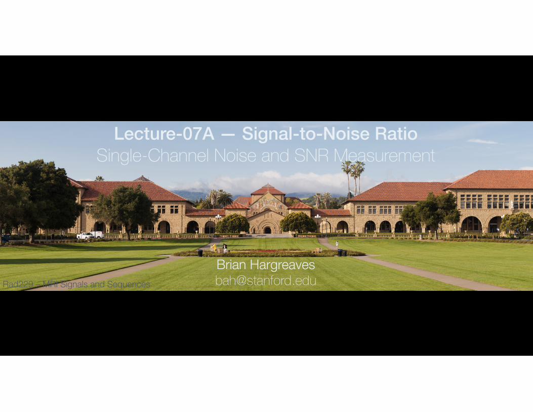
Brian Hargreaves [email protected]
Lecture-07A — Signal-to-Noise Ratio Single-Channel Noise and SNR Measurement

Learning Objectives
• Understand noise statistics in k-space, complex images, and magnitude images
• Explain when the distribution is Gaussian, Rayleigh and Rician
• Know basic methods to measure SNR
Rad229
3Lec-07ASlide-

SNR: Signal-to-Noise Ratio
•Signal (desired) vs Noise (interference)•Thermal noise, depends on coil, patient size
Rad229
4Lec-07ASlide-
Low SNR High SNR
Signal
Noise
Real
Imag
inary

Origins of SNR
• Body noise dominance • SNR = C f(Ob) (Im)
– C = constants– f(Ob) = function of object– Im = Imaging parameters
Macovaki A, Noise in MRI. Magn Reson Med 1996; 36:494-497Rad229
5Lec-07ASlide-
SNR = [2χ ρ
γμ0 KTπ ] 1
r20 l [ω0Vvoxel Tacq]
ω0 = frequency Vvoxel = voxel volumeTacq = A/D time

Noise and the Signal Equation
• Noise is zero-mean, complex, additive• Recall signal equation from lecture 2:
• Additive complex, gaussian noise:• Probability density function P(nr,ni) is a simple product of
gaussian distributions for real and imaginary:
Noise is complex, gaussian and additive, with zero mean and variance σ2 (both real and imaginary)Rad229
6Lec-07ASlide-
S( k ) = ∫objectM( r )e−i2π k ⋅ r d r + nc(0,σ)
( 1
σ 2πe− n2
i2σ2 )( 1
σ 2πe− n2r
2σ2 )P(nr, ni) =
nc = nr + i * ni

Gaussian Noise in (Discrete) Image Space and k-Space
• Assume equally scaled FFT / iFFT: – Equations are 1D!
• Noise statistics preserved (Mn <=> Sk)– additive complex noise– gaussian, zero-mean
Complex, zero-mean gaussian noise in k-space transforms to complex gaussian noise in image space, both same variance σ2
Rad229
7Lec-07ASlide-
Sk =1
N
N−1
∑n=0
Mne−i2πkn/N
Mn =1
N
N−1
∑k=0
Sei2πkn/N
σ = σr = σi

Example: Verifying Noise Properties
• Make k-space noise, Fourier transform, calculate statistics for varying signal:
lec7_01.mRad229
8Lec-07ASlide-
nsig = 1; % Noise sigma parameter (real and imaginary)N = 256; % Image/k-space size.
kr = randn([N,N])*nsig; % Generate gaussian noise (real part)ki = randn([N,N])*nsig; % Generate gaussian noise (imag part, same)k = kr+i*ki; % Combine
im = N * ift(k); % iFFT with scaling of sqrt(N*N)=N[std(real(im(:))),std(imag(im(:)))]
% -- Calculate noise as a function of SNR, with magnitude images
s=[0:0.1:10]; % s = Signal, so same as SNR if nsig==1for p=1:length(s) mn(p) = mean(abs(im(:)+s(p))); % Mean of magnitude signal sd(p) = std(abs(im(:)+s(p))); % Std.deviation of magnitude end;
k-Space Image
Close to gaussian (SNR>4)
Question 1
If the k-space of a 128x128 image is all 1s, and the noise has σ=1, what is the SNR at the image center? What is the mean of the magnitude background image?
Noise transfers without scaling, so has σ=1 in the imageThe signal at the center is the sum over 128x128, normalized by N, or 128SNR = 128The background mean is
Rad229
9Lec-07ASlide-
σ π/2 = 1.2
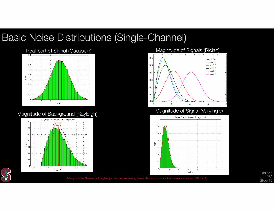
Basic Noise Distributions (Single-Channel)
Magnitude Noise is Rayleigh for zero-mean, then Rician (Looks Gaussian above SNR ~ 4)Rad229
10Lec-07ASlide-
Real-part of Signal (Gaussian) Magnitude of Signals (Rician)
Magnitude of Signal (Varying ν)Magnitude of Background (Rayleigh)
π/2

Question 2
Intuitively, why is the noise distribution for magnitude images almost gaussian for reasonably high SNR?
A. The “quadrature” noise has minimal effect on magnitudeB. The noise is real-valued in image spaceC. The image and noise are in-phase
A. Quadrature noise does not affect magnitude much
Rad229
11Lec-07ASlide-
Signal
Noise
Real
Imag
inary

Basic SNR Measurement (1 coil)
• Measure mean in signal area ROI• Measure std-deviation in magnitude
background ROI• Correct for Rayleigh distribution in background
For a single channel coil, noise can be measured from the background magnitude mean or standard deviationRad229
12Lec-07ASlide-
meanRayleigh = 1.26 σRayleigh = 0.65
σgaussian = meanRayleigh / sqrt(π/2) = 1.008 σgaussian = σRayleigh / sqrt(2-π/2) = 0.997

Difference Method SNR
• In theory, N measurements should give you a population, and at each pixel you get a (roughly gaussian) distribution
• With 2 measurements you can still estimate mean and standard deviation (Reeder et al)
• Still want SNR > 4, or underestimate noise
The difference method is a crude measure of the variation at a particular voxelRad229
13Lec-07ASlide-
Sum
Difference of Magnitude Images
σMag-Diff = 1.394 σgaussian = σMag-Diff/ sqrt(2) ~ 1.0

Question 3
If you acquire an image 3 times and the standard deviation of the magnitude signals is 0.5 and the average signal is 5
A. The SNR is about 10, and noise is Rayleigh distributedB. The SNR is about 10, noise is approximately GaussianC. The SNR is about 7, and noise is complex-gaussianD. SNR is about 7, and noise is approximately Gaussian
B. Above SNR of ~4 the Rician distribution looks Gaussian, so this method will work well
Rad229
14Lec-07ASlide-
Magnitude of Signals

Summary
• Noise in k-space and complex images is complex and Gaussian• Magnitude image noise has:
– Rician distribution (non-zero signal or mean)– Rayleigh in the background)
• SNR can be measured by foreground/background or the difference method (with corrections as appropriate)
Rad229
15Lec-07ASlide-
How do different setup factors and sequence parameters affect SNR?
Copyright © 2022 FDOKUMEN

