


Bahasa
Halaman
Hukum

Photo-z optimization for measurements of the BAOradial scale
Daniel Roig1, Licia Verde3,1, Jordi Miralda-Escude3,2,1,Raul Jimenez3,1, Carlos Pena-Garay4
1 Institute of Space Sciences (CSIC-IEEC), Fac. Ciencies, CampusUAB, Bellaterra, Spain.2 Institut of Ciencies del Cosmos, Universitat de Barcelona,Barcelona, Spain.3 ICREA, Barcelona, Spain4 Instituto de Fısica Corpuscular (CSIC-UVEG), Valencia, Spain
Abstract.Baryon Acoustic Oscillations (BAO) in the radial direction offer a method
to directly measure the Universe expansion history, and to set limits to spacecurvature when combined to the angular BAO signal. In addition to spectroscopicsurveys, radial BAO might be measured from accurate enough photometricredshifts obtained with narrow-band filters. We explore the requirements fora photometric survey using Luminous Red Galaxies (LRG) to competitivelymeasure the radial BAO signal and discuss the possible systematic errors ofthis approach. If LRG were a highly homogeneous population, we show thatthe photo-z accuracy would not substantially improve by increasing the numberof filters beyond ∼ 10, except for a small fraction of the sources detected athigh signal-to-noise, and broad-band filters would suffice to achieve the targetσz = 0.003(1 + z) for measuring radial BAO. Using the LRG spectra obtainedfrom SDSS, we find that the spectral variability of LRG substantially worsens theachievable photometric redshift errors, and that the optimal system consists of∼ 30 filters of width ∆λ/λ ∼ 0.02. A S/N > 20 is generally necessary at thefilters on the red side of the Hα break to reach the target photometric accuracy.We estimate that a 5-year survey in a dedicated telescope with etendue in excessof 60 m2 deg2 would be necessary to obtain a high enough density of galaxies tomeasure radial BAO with sufficiently low shot noise up to z = 0.85. We concludethat spectroscopic surveys have a superior performance than photometric ones formeasuring BAO in the radial direction.
1. Introduction
An important observable to constrain the nature of dark energy is the HubbleparameterH(z) [1], since it constitutes a more direct probe to the dark energy equationof state than the angular diameter distance da(z) or the luminosity distance dL(z),which depend on an integral of H(z). Einstein’s equations imply that a homogeneousand isotropic universe, which is described by the FRW metric, that is composed ofmatter and dark energy with equation of state pQ = wQ(z)ρQ expands according to
H(z)H0
=[ρT (z)ρT (0)
]1/2
= (1)
arX
iv:0
812.
3414
v2 [
astr
o-ph
] 1
8 Ja
n 20
09
Photo-z optimizaton 2[ΩM (1 + z)3 + Ωk(1 + z)2 + ΩQ exp
(3∫ z
0
1 + wQ(z′)1 + z′
dz′)]1/2
,
where the subscripts Q, k, M and T refer to dark energy, space curvature, matter, andtotal energy density, respectively. In the absence of space curvature, the quantitiesdA(z) and dL(z) are related to H(z) via dA(z)(1 + z) = dL(z)/(1 + z) =
∫ z0dz′/H(z′).
The acoustic oscillations in the photon-baryon plasma, observed as acoustic peaksin the CMB power spectrum, are also imprinted in the matter distribution at thescale of the sound horizon at the radiation drag epoch, when baryons were releasedfrom the photon pressure. The mass distribution is traced by the distribution ofgalaxies, and the Baryon Acoustic Oscillations (BAO) can be observed as a peak inthe galaxy correlation function or as a series of harmonic oscillations in the galaxypower spectrum. The sound horizon at the radiation drag epoch can be computed veryaccurately from CMB observations (e.g., rs = 153.2± 2.0 Mpc from WMAP5, [2]), soit provides a natural standard ruler. In fact, the galaxy power spectrum can be usedto measure both the angular diameter distance through the clustering perpendicularto the line-of-sight, and the expansion rate H(z) through the clustering along the line-of-sight. Therefore, BAO measurements test the relation between H(z) and dA(z),providing constraints on dark energy and a limit to space curvature (e.g., [3, 4, 5, 6] ).The BAO technique is being considered a powerful probe to the nature of dark energy[7, 8, 9, 10] because of its potential to provide a standard ruler at different redshiftsand its robustness to systematic effects.
For an ideal galaxy survey, [11] have shown that a volume of 1 (Gpc/h)3 at lowredshift can constrain H0 to the 7 % level. Forthcoming surveys with larger volumeare expected to reach the statistical power to constrain H(z) at the % level. Thereare a number of requirements that these surveys need to satisfy for measuring BAO:covering a large survey volume, modeling the effects of galaxy bias and non-linearity,characterizing the covariance between different modes, evaluating the galaxy selectionfunction to sufficient accuracy, reducing photometric calibration errors to low enoughlevels to avoid contamination of the BAO signal, etc. Measuring the BAO scalein the radial direction demands in addition that galaxy redshifts are measured to asufficiently high accuracy, σz, to avoid an excessive smoothing of the BAO peak, whichhas an intrinsic width δr ∼ 10 Mpc, i.e., δz ≤ δrH(z)/c. As shown by [12], a redshiftaccuracy σz < 0.003(1 + z) is required to avoid substantial loss of accuracy of theH(z) measurement from a given survey volume. Spectroscopic surveys usually yielda redshift accuracy much higher than this minimum requirement.
An alternative approach to measure the large number of redshifts requiredfor BAO detection are photometric redshifts from imaging surveys. Broad-bandphotometry with ∼ 6 filters usually reaches only to σz/(1 + z) ∼ 0.03 for the generalpopulation (with red galaxies having slightly smaller photo-z errors than blue ones),insufficient for measuring radial BAO. However, as the Combo-17 survey [13] hasdemonstrated, the galaxy photo-z accuracy can be improved by using a larger numberof narrower filters. Photometric surveys can cover a large area of the sky fasterthan a spectroscopic survey and reach a higher number density of observed objects.We are therefore motivated to investigate the requirements for a photometric surveywith medium to narrow bands to deliver interesting BAO measurements, and theoptimization of the number of filters. Previous work has already explored this issue([14, 12, 15, 16]). Here we concentrate specifically on the impact of the number ofbands, signal-to-noise, and non-uniformity of the galaxy sample. We conclude with
Photo-z optimizaton 3
several considerations on the systematic effects that the photometric approach entails.In our investigation we use both synthetic stellar population models and Sloan
Digital Sky Survey (SDSS)-DR6 spectra of Luminous Red Galaxies. We concentrateon LRG because they have several properties that make them particularly useful forBAO surveys: they are a fairly homogeneous population, the form of their spectramakes them particularly suitable for good photo-z determinations, and their highluminosity facilitates reaching a high enough signal-to-noise up to high redshifts. Forthese reasons, LRG are the target of choice for z < 2 BAO surveys (at higher redshiftthe Lyα forest probably provides the best method for measuring BAO; see [17]). Themain conclusion we reach is that a spectroscopic survey is superior to narrow-bandphotometric surveys for measuring the radial BAO signal. We also show that if itwere possible to find a very homogeneous population of LRG (with spectra closelymatched by a single spectral template), then the photometric redshift accuracy wouldnot substantially increase with the number of filters used beyond a total number of∼ 10 at a fixed total exposure time. This is not the case for galaxies measured at highsignal-to-noise, for which a larger number of filters is optimal, but this high signal-to-noise cannot be achieved for a large enough number of objects in a way that iscompetitive with the spectroscopic approach. In reality, however, the variability ofrealistic galaxy spectra worsens the photometric redshift accuracy, making it optimalto increase the number of filters to ∼ 30 and requiring a higher signal-to-noise per filterto reach the desired redshift accuracy. These results are generally in good agreementwith those of [15].
This paper is organized as follows: in § 2 we review the requirements for a surveyto measure radial BAO. The modeling of the LRG population is described in § 3, andin § 4 we describe our fiducial survey model. The results are presented in § 5, wherewe analyze in detail the photo-z accuracy as a function of the number of filters, galaxyluminosity and redshift, first for ideal galaxies that match the templates precisely andthen for real galaxies with SDSS spectra. Discussion and conclusions are presented in§ 6 and § 7. Throughout this paper, we use a cosmological model with H0 = 70 km s−1
Mpc−1, Ωm = 0.3, ΩΛ = 0.7. Readers who want to quickly see the main conclusionsor our study may wish to go directly to Figure 14. This shows the number density ofLRG in several redshift bins with photometric redshift better than 0.003(1 + z) as afunction of the etendue times the exposure time of a survey. It also shows the numberdensity required to reach nP = 1, necessary to make shot noise subdominant in theFourier modes near the line-of-sight useful for measuring BAO.
2. Spectroscopy vs photometry and target photometric requirements
Future BAO surveys need to: a) cover large volumes of the universe samplingthe acoustic scale rs = 153.2 ± 2 Mpc with a density of galaxies high enough tomake shot-noise subdominant, and b) not degrade with redshift errors the line-of-sight information that yields a measurement of H(z). The latter conditionimplies, quantitatively, that the statistical photo-z errors need to be smaller thanσz = 0.003(1 + z) [12]. In Figure 1 we show the present–day (z=0) linear matterpower spectrum (dotted line) and the corresponding line-of-sight redshift-space powerspectrum (thin solid line), assuming a scale-independent bias b = 2, a β parameterβ = 1/b d ln δ/d ln a ∼ Ω0.6
m /b ' 0.24, and assuming an intrinsic galaxy velocitydispersion of 420 km/s, corresponding to a pairwise velocity dispersion σp = 600km/s,typical of non-linear redshift-space distortions. The line-of-sight power spectrum
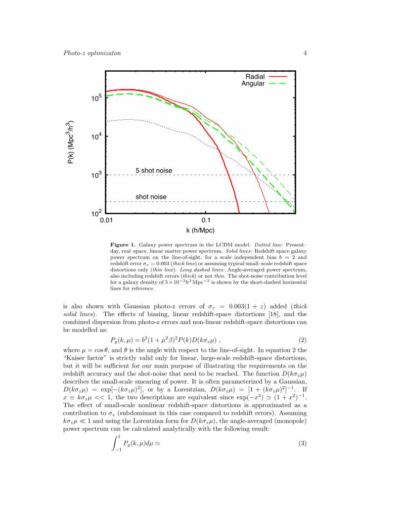
Photo-z optimizaton 4
102
103
104
105
0.01 0.1
P(k)
(Mpc
3 /h3 )
k (h/Mpc)
shot noise
5 shot noise
RadialAngular
Figure 1. Galaxy power spectrum in the LCDM model. Dotted line: Present–day, real–space, linear matter power spectrum. Solid lines: Redshift space galaxypower spectrum on the line-of-sight, for a scale independent bias b = 2 andredshift error σz = 0.003 (thick line) or assuming typical small–scale redshift spacedistortions only (thin line). Long dashed lines: Angle-averaged power spectrum,also including redshift errors (thick) or not thin. The shot-noise contribution levelfor a galaxy density of 5×10⁻³h3 Mpc−3 is shown by the short-dashed horizontallines for reference.
is also shown with Gaussian photo-z errors of σz = 0.003(1 + z) added (thicksolid lines). The effects of biasing, linear redshift-space distortions [18], and thecombined dispersion from photo-z errors and non-linear redshift-space distortions canbe modelled as:
Pg(k, µ) = b2(1 + µ2β)2P (k)D(kσzµ) , (2)
where µ = cos θ, and θ is the angle with respect to the line-of-sight. In equation 2 the“Kaiser factor” is strictly valid only for linear, large-scale redshift-space distortions,but it will be sufficient for our main purpose of illustrating the requirements on theredshift accuracy and the shot-noise that need to be reached. The function D(kσzµ)describes the small-scale smearing of power. It is often parameterized by a Gaussian,D(kσzµ) = exp[−(kσzµ)2], or by a Lorentzian, D(kσzµ) = [1 + (kσzµ)2]−1. Ifx ≡ kσzµ << 1, the two descriptions are equivalent since exp(−x2) ' (1 + x2)−1.The effect of small-scale nonlinear redshift-space distortions is approximated as acontribution to σz (subdominant in this case compared to redshift errors). Assumingkσzµ 1 and using the Lorentzian form for D(kσzµ), the angle-averaged (monopole)power spectrum can be calculated analytically with the following result:∫ 1
−1
Pg(k, µ)dµ ' (3)

Photo-z optimizaton 5
b2P (k)[
(β2 + 6β)3k2σ2
z
− β4
k4σ4z
+(
1kσz− β√
8k3σ3z
+β2
√2k5σ5
z
)arctan(kσz)
].
This monopole term is shown as the long-dashed line in Figure 1. The Figurealso shows the shot noise contribution (short-dashed lines) for a galaxy density ofn = 5 × 10⁻³, and the level at which nP = 5 and nP = 1 , which is where theshot noise contribution is negligible: in the line-of-sight, shot noise starts becomingcomparable to the P (k) signal at larger scales than for the angle-averaged P (k).
Let us consider the following two cases: a photometric survey with targetphoto-z errors σz ∼ 0.003 (thick lines), and a spectroscopic survey (thinlines, corresponding to unavoidable non-linear velocities). The sampling varianceerror on P (k, µ) scales as σP /P = 1/
√2πk2∆k∆µVeff/(2π)3, where Veff =
[nP (k, µ)/(nP (k, µ) + 1)]2 Vsurvey, and the accuracy at which the acoustic scale canbe measured is directly proportional to σP /P . Thus, if the two surveys have thesame number density of galaxies, and the spectroscopic survey reaches nP = 5 alongthe line of sight at k = 0.32h/Mpc, then the photometric survey reaches nP = 5 atk = 0.16h/Mpc. Note that the number of independent modes is roughly proportionalto k3
max, and so the spectroscopic survey could obtain a much better constraint onthe BAO scale from measuring the power on many more modes. ‡ In order to becompetitive with a spectroscopic survey, a photometric survey would need to achievea much higher galaxy density. If the survey volume were to be the same for the twosurveys, then at k = 0.2h/Mpc a photometric survey would need a galaxy numberdensity exp(−k2σ2
z) ∼ 25 times higher than a spectroscopic survey to achieve the samenP along the line of sight direction. The angle-averaged quantity is, of course, lesssensitive to the smearing along the line of sight, and the same is true for all orientationswhere µ < 1. As shown by [12], at z∼1 a redshift error of 0.3% degrades the erroron H(z) by a factor ∼ 2, demanding therefore a survey with 4 times the volume ofa spectroscopic survey to match its performance. As most forthcoming spectroscopicsurveys will cover more than a quarter of the available sky (i.e., more than a quarter ofthe 30000 square degrees outside the galactic plane), the photometric approach mightonly be advantageous if it could reach higher redshifts.
The above considerations indicate that a spectroscopic survey is the favoredoption unless a much larger fraction of the sky can be covered with a photometricsurvey and with an extremely high object density; this is equivalent to imposing therequirement of σz < 0.3% down to fainter magnitudes. Below, we calculate if such asurvey is possible. For this we concentrate on LRG, which are bright and have veryhomogeneous spectra, and we study the dependence of the results on intrinsic galaxyvariability, luminosity, etc.
3. Models for the Population of Luminous Red Galaxies
We start by calculating the number density of LRG that can be observed at eachluminosity and redshift. We use the [19] luminosity function of LRG and adopttheir model of a Shechter luminosity function slope of α = −0.5 (see Table 6 in[19]). To model the spectral distribution of galaxies, we use the first five templatespresented in [20] §. These are empirical templates computed using the SPEED [21]
‡ Since the relative error on the power spectrum σP /P does not depend on redshift, the aboveconsiderations are valid at any redshift, with the caveat that the non-linearities decrease with z butthe photo-z errors do not.§ http://www.ice.csic.es/personal/jimenez/PHOTOZ/
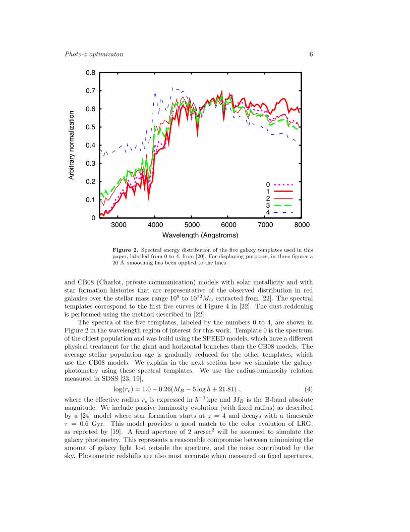
Photo-z optimizaton 6
0
0.1
0.2
0.3
0.4
0.5
0.6
0.7
0.8
3000 4000 5000 6000 7000 8000
Arbi
trary
nor
mal
izatio
n
Wavelength (Angstroms)
01234
Figure 2. Spectral energy distribution of the five galaxy templates used in thispaper, labelled from 0 to 4, from [20]. For displaying purposes, in these figures a20 A smoothing has been applied to the lines.
and CB08 (Charlot, private communication) models with solar metallicity and withstar formation histories that are representative of the observed distribution in redgalaxies over the stellar mass range 109 to 1012M extracted from [22]. The spectraltemplates correspond to the first five curves of Figure 4 in [22]. The dust reddeningis performed using the method described in [22].
The spectra of the five templates, labeled by the numbers 0 to 4, are shown inFigure 2 in the wavelength region of interest for this work. Template 0 is the spectrumof the oldest population and was build using the SPEED models, which have a differentphysical treatment for the giant and horizontal branches than the CB08 models. Theaverage stellar population age is gradually reduced for the other templates, whichuse the CB08 models. We explain in the next section how we simulate the galaxyphotometry using these spectral templates. We use the radius-luminosity relationmeasured in SDSS [23, 19],
log(re) = 1.0− 0.26(MB − 5 log h+ 21.81) , (4)
where the effective radius re is expressed in h−1 kpc and MB is the B-band absolutemagnitude. We include passive luminosity evolution (with fixed radius) as describedby a [24] model where star formation starts at z = 4 and decays with a timescaleτ = 0.6 Gyr. This model provides a good match to the color evolution of LRG,as reported by [19]. A fixed aperture of 2 arcsec2 will be assumed to simulate thegalaxy photometry. This represents a reasonable compromise between minimizing theamount of galaxy light lost outside the aperture, and the noise contributed by thesky. Photometric redshifts are also most accurate when measured on fixed apertures,

Photo-z optimizaton 7
0.2
0.3
0.4
0.5
0.6
0.7
0.8
0.5 1 1.5 2 2.5 3 3.5 4 4.5 5
Frac
tion
of lig
ht in
side
a 2
arcs
ec2 a
pertu
re
L/L*
Seeing of 0.8 arcsecSeeing of 1.2 arcsec
Figure 3. Fraction of light of a LRG within a 2 arcsec2 aperture as a function ofluminosity for four different values of redshift, z = 0.3, 0.5, 0.7, 0.9 from bottomto top, and two different values of the seeing, 0.8 arcsec (solid lines) and 1.2 arcsec(dotted lines).
rather than variable apertures that may be adjusted to the observed galaxy profile.We show in Figure 3 the fraction of galaxy light included within the aperture as afunction of luminosity for four different values of redshift and two different seeings.
4. Survey Model
Throughout this paper we consider a fiducial narrow-band photometric survey as anexample of the accuracy that can be achieved to measure a large number of LRGphotometric redshifts, for the purpose of detecting BAO. We focus on narrow-bandphotometry in a wavelength range that is most useful for obtaining LRG redshifts overthe range z = 0.5 to z = 1.0, using the 4000 A (or Hα) break, a blend of H and Ca lines.We choose a set of Nf filters covering the fixed wavelength range from λ1 = 5300 A toλn = 8300 A, dividing this range into Nf intervals of equal wavelength width. We willconsider different values Nf to optimize this number for photometric redshifts for agiven survey and telescope setup. The shape of the filter window functions is assumedto be a top-hat of width ∆λ = (λn − λ1)/(Nf + 1/2)‖, with the addition of lateralwings on each side where the window function varies linearly from zero to the valuein the central top-hat. The width of each of the wings is set to 1/4 of the width of thetop-hat. The top-hat parts of the window function are adjacent and non-overlapping,whereas the wings cause the filters to have a certain degree of overlap. In a practical
‖ The 1/2 is due to the presence of the wings.

Photo-z optimizaton 8
0.2
0.25
0.3
0.35
0.4
0.45
0.5
0.55
0.6
0.65
0.7
5500 6000 6500 7000 7500 8000
Thro
ughp
ut
Wavelength (Angstroms)
Figure 4. Overall throughput (solid) and throughput without includingatmospheric absorption (dotted) used in this work.
application, it would probably be useful to complement this filter system with widerfilters around the wavelength range considered here: this would eliminate some of thephoto-z catastrophic failures (outliers in the photometric redshift error distribution).However, the addition of wide filters would not improve the accuracy of the goodredshifts because they cannot contribute to a better resolution.
Figure 4 shows the overall throughput as a function of wavelength. We haveincluded atmospheric absorption assuming an average of 1.2 atmospheric columns.We also include two mirror reflections, filter transmission and CCD efficiency from[26, 27, 28]. We use the sky brightness of Patat (2008, private communication; [25]),measured for the Paranal Observatory, to simulate the photometric noise in eachband. This is adequate for a dark site in the absence of any artificial light, and amean airglow intensity over the solar cycle. Figure 5 shows the spectrum of the sky inthe AB magnitude system, and the average sky brightness in each one of the filters forthe case Nf = 30 (blue diamonds). The squares and circles indicate the noise levels inour fiducial survey and are discussed below.
Once the shape of the filters, the overall throughput, sky brightness, source fluxand radius, and seeing have been fixed, the photometric precision reached by a surveyfor the flux in each filter is proportional to [Et/(NfΩ)]1/2, where E is the etendue(the product of the effective telescope aperture times the field of view), t is the totalsurvey observing time, and Ω is the total solid angle covered by the survey. We shallassume for our fiducial survey a product Et = 1.5 × 10⁵ m2 deg2 hr, correspondingfor example to a characteristic case of a dedicated telescope with etendue E = 30(e.g., a 3 m telescope with a 5 square degrees field of view) that can obtain good
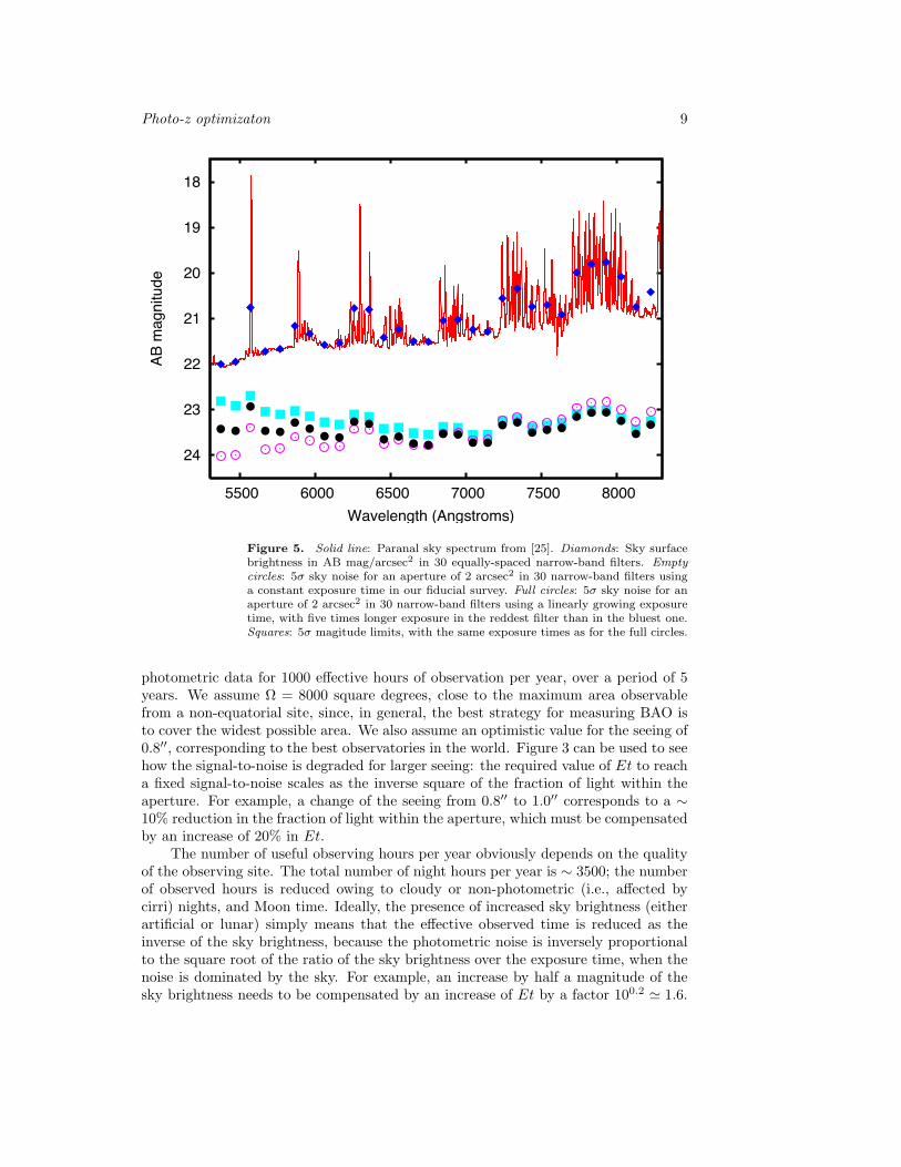
Photo-z optimizaton 9
18
19
20
21
22
23
24
5500 6000 6500 7000 7500 8000
AB m
agni
tude
Wavelength (Angstroms)
Figure 5. Solid line: Paranal sky spectrum from [25]. Diamonds: Sky surfacebrightness in AB mag/arcsec2 in 30 equally-spaced narrow-band filters. Emptycircles: 5σ sky noise for an aperture of 2 arcsec2 in 30 narrow-band filters usinga constant exposure time in our fiducial survey. Full circles: 5σ sky noise for anaperture of 2 arcsec2 in 30 narrow-band filters using a linearly growing exposuretime, with five times longer exposure in the reddest filter than in the bluest one.Squares: 5σ magitude limits, with the same exposure times as for the full circles.
photometric data for 1000 effective hours of observation per year, over a period of 5years. We assume Ω = 8000 square degrees, close to the maximum area observablefrom a non-equatorial site, since, in general, the best strategy for measuring BAO isto cover the widest possible area. We also assume an optimistic value for the seeing of0.8′′, corresponding to the best observatories in the world. Figure 3 can be used to seehow the signal-to-noise is degraded for larger seeing: the required value of Et to reacha fixed signal-to-noise scales as the inverse square of the fraction of light within theaperture. For example, a change of the seeing from 0.8′′ to 1.0′′ corresponds to a ∼10% reduction in the fraction of light within the aperture, which must be compensatedby an increase of 20% in Et.
The number of useful observing hours per year obviously depends on the qualityof the observing site. The total number of night hours per year is ∼ 3500; the numberof observed hours is reduced owing to cloudy or non-photometric (i.e., affected bycirri) nights, and Moon time. Ideally, the presence of increased sky brightness (eitherartificial or lunar) simply means that the effective observed time is reduced as theinverse of the sky brightness, because the photometric noise is inversely proportionalto the square root of the ratio of the sky brightness over the exposure time, when thenoise is dominated by the sky. For example, an increase by half a magnitude of thesky brightness needs to be compensated by an increase of Et by a factor 100.2 ' 1.6.
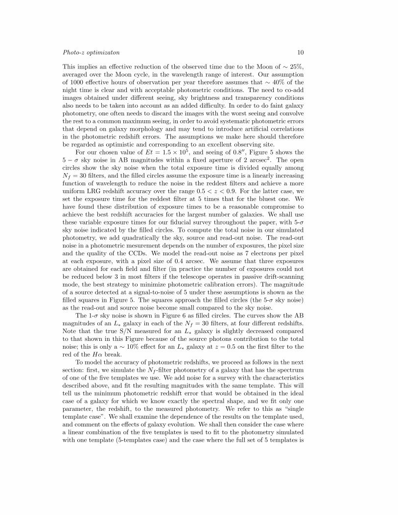
Photo-z optimizaton 10
This implies an effective reduction of the observed time due to the Moon of ∼ 25%,averaged over the Moon cycle, in the wavelength range of interest. Our assumptionof 1000 effective hours of observation per year therefore assumes that ∼ 40% of thenight time is clear and with acceptable photometric conditions. The need to co-addimages obtained under different seeing, sky brightness and transparency conditionsalso needs to be taken into account as an added difficulty. In order to do faint galaxyphotometry, one often needs to discard the images with the worst seeing and convolvethe rest to a common maximum seeing, in order to avoid systematic photometric errorsthat depend on galaxy morphology and may tend to introduce artificial correlationsin the photometric redshift errors. The assumptions we make here should thereforebe regarded as optimistic and corresponding to an excellent observing site.
For our chosen value of Et = 1.5 × 10⁵, and seeing of 0.8′′, Figure 5 shows the5 − σ sky noise in AB magnitudes within a fixed aperture of 2 arcsec2. The opencircles show the sky noise when the total exposure time is divided equally amongNf = 30 filters, and the filled circles assume the exposure time is a linearly increasingfunction of wavelength to reduce the noise in the reddest filters and achieve a moreuniform LRG redshift accuracy over the range 0.5 < z < 0.9. For the latter case, weset the exposure time for the reddest filter at 5 times that for the bluest one. Wehave found these distribution of exposure times to be a reasonable compromise toachieve the best redshift accuracies for the largest number of galaxies. We shall usethese variable exposure times for our fiducial survey throughout the paper, with 5-σsky noise indicated by the filled circles. To compute the total noise in our simulatedphotometry, we add quadratically the sky, source and read-out noise. The read-outnoise in a photometric mesurement depends on the number of exposures, the pixel sizeand the quality of the CCDs. We model the read-out noise as 7 electrons per pixelat each exposure, with a pixel size of 0.4 arcsec. We assume that three exposuresare obtained for each field and filter (in practice the number of exposures could notbe reduced below 3 in most filters if the telescope operates in passive drift-scanningmode, the best strategy to minimize photometric calibration errors). The magnitudeof a source detected at a signal-to-noise of 5 under these assumptions is shown as thefilled squares in Figure 5. The squares approach the filled circles (the 5-σ sky noise)as the read-out and source noise become small compared to the sky noise.
The 1-σ sky noise is shown in Figure 6 as filled circles. The curves show the ABmagnitudes of an L∗ galaxy in each of the Nf = 30 filters, at four different redshifts.Note that the true S/N measured for an L∗ galaxy is slightly decreased comparedto that shown in this Figure because of the source photons contribution to the totalnoise; this is only a ∼ 10% effect for an L∗ galaxy at z = 0.5 on the first filter to thered of the Hα break.
To model the accuracy of photometric redshifts, we proceed as follows in the nextsection: first, we simulate the Nf -filter photometry of a galaxy that has the spectrumof one of the five templates we use. We add noise for a survey with the characteristicsdescribed above, and fit the resulting magnitudes with the same template. This willtell us the minimum photometric redshift error that would be obtained in the idealcase of a galaxy for which we know exactly the spectral shape, and we fit only oneparameter, the redshift, to the measured photometry. We refer to this as “singletemplate case”. We shall examine the dependence of the results on the template used,and comment on the effects of galaxy evolution. We shall then consider the case wherea linear combination of the five templates is used to fit to the photometry simulatedwith one template (5-templates case) and the case where the full set of 5 templates is
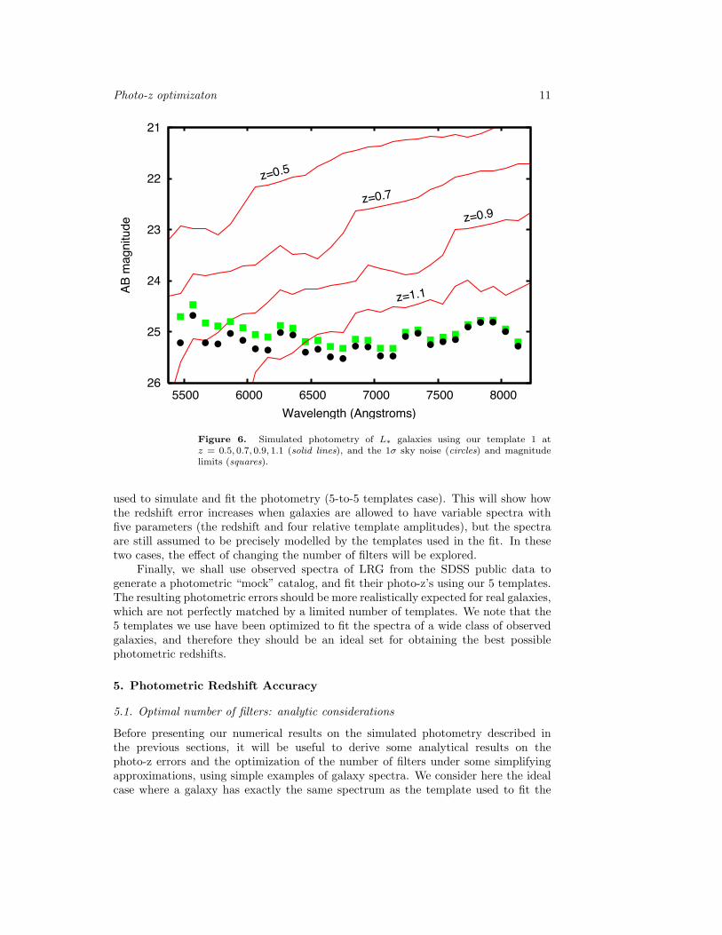
Photo-z optimizaton 11
21
22
23
24
25
26 5500 6000 6500 7000 7500 8000
AB m
agni
tude
Wavelength (Angstroms)
z=0.5
z=0.7
z=0.9
z=1.1
Figure 6. Simulated photometry of L∗ galaxies using our template 1 atz = 0.5, 0.7, 0.9, 1.1 (solid lines), and the 1σ sky noise (circles) and magnitudelimits (squares).
used to simulate and fit the photometry (5-to-5 templates case). This will show howthe redshift error increases when galaxies are allowed to have variable spectra withfive parameters (the redshift and four relative template amplitudes), but the spectraare still assumed to be precisely modelled by the templates used in the fit. In thesetwo cases, the effect of changing the number of filters will be explored.
Finally, we shall use observed spectra of LRG from the SDSS public data togenerate a photometric “mock” catalog, and fit their photo-z’s using our 5 templates.The resulting photometric errors should be more realistically expected for real galaxies,which are not perfectly matched by a limited number of templates. We note that the5 templates we use have been optimized to fit the spectra of a wide class of observedgalaxies, and therefore they should be an ideal set for obtaining the best possiblephotometric redshifts.
5. Photometric Redshift Accuracy
5.1. Optimal number of filters: analytic considerations
Before presenting our numerical results on the simulated photometry described inthe previous sections, it will be useful to derive some analytical results on thephoto-z errors and the optimization of the number of filters under some simplifyingapproximations, using simple examples of galaxy spectra. We consider here the idealcase where a galaxy has exactly the same spectrum as the template used to fit the
Photo-z optimizaton 12
measured photometry, and approximate the filter windows as a top-hat.If a fixed total exposure time is to be divided among all the filters, then the signal-
to-noise in each individual filter, F/σF (where F denotes flux and σF its statisticalerror), is inversely proportional to the number of filters Nf : the exposure time ineach filter is tf ∝ N−1
f , and the wavelength width of each filter is ∆λ ∝ N−1f .
Hence, the number of photons detected in each filter is Nph ∝ tf∆λ ∝ N−2f , and
F/σF ∝ N1/2ph ∝ N−1
f . As we increase the number of filters, the resolution increasesat the expense of the achieved signal-to-noise.
To model the use of the Hα break in LRG, we first consider a galaxy spectrumthat has a break at wavelength λ0, where the flux per unit wavelength is Fλ = F0 atλ > λ0 and Fλ = (1−B)F0 at λ < λ0. The filter that includes the break wavelengthλ0 has a flux
F = F0(1−Bx) , (5)
where x = (λi−λ0)/∆λ, and λi is the wavelength of the right edge of the filter. Fromthe measured value of F (and assuming that we know exactly the values of F0 and Bfrom the measurements in the other filters), the wavelength λ0 can be measured to anaccuracy
σλ = ∆λσFF0B
. (6)
Since σF /F0 ∝ Nf , and ∆λ ∝ N−1f , we conclude that the error to which the
wavelength λ0 is measured is independent of the number of filters, and results ina photometric redshift accuracy σz given by
σz1 + z
≡ σlz =σλλ
=∆λλ
σFF0B
. (7)
In other words, unresolved breaks in the spectra of galaxies yield a redshiftmeasurement that does not improve as the number of filters is increased. This iscorrect only in the idealized situation where the amplitude of the break is perfectlyknown and galaxy variability may be ignored.
For a resolved break, we assume that the flux varies linearly from F0 to F0(1−B)over a wavelength range λ0 to λ0 + δλ. The flux measured in a filter centered atwavelength λi and which is fully included within the interval of the break of widthδλ is F = F0(1 − Bx), where x = (λi − λ0)/δλ. Hence, the error on λ0 that can bededuced from the flux measured in one filter only is
σλ = δλσFF0B
∝ Nf . (8)
Since the number of filters contained in the wavelength range of the resolved break,δλ, is proportional to Nf , and the combined error from the measurement in all thefilters is reduced as N−1/2
f , we find that the set of all photometric measurements will
yield an error σλ ∝ N1/2f . Therefore, the filters should not be any narrower than the
intrinsic width of any breaks that substantially contribute to the photometric redshiftmeasurement.
On the other hand, if the spectrum contains features similar to an emission orabsorption line, then it is advantageous to increase the number of filters. For a linefeature with an equivalent width Wλ which is entirely contained in one filter, themeasured flux is F = F0(1 +Wλ/∆λ), independently of the position of the line withina top-hat filter. The difference F − F0 = F0Wλ/∆λ ∝ Nf can be measured to an
Photo-z optimizaton 13
accuracy σF ∝ Nf , so the position of the feature is measured to increasing accuracyas the number of filters is increased, up to the point where the feature is resolved.
In practice, the spectra of LRG contain several features that may beapproximately modelled as breaks and/or line features of different wavelength widths.In the case of a single template, the optimal number of filters results from thecontribution of all the features to the determination of the photometric redshift. Atthe same time, the spectra of real galaxies are, of course, not described by a singletemplate and depend on a variety of parameters. The need to fit for these spectralvariations in addition to the redshift favors an increased number of filters when thesignal-to-noise that can be reached is high enough. This is seen in more detail inthe following section; the analytic considerations discussed above will be helpful tointerpret the numerical results for fits to simulated photometry of LRG.
5.2. Single template galaxies
We now present the numerical results of recovering photometric redshifts from thesimulated photometry of LRG spectra, for the case of our fiducial survey as describedin §4. The distribution of photometric redshift errors is generally not Gaussian becauseof the presence of outliers, or catastrophic failures, which naturally increase as thesignal-to-noise drops. To avoid having to deal with identification of outliers, we reportthe photo-z error σz in all of our figures, unless otherwise stated, as the interval suchthat 68% of the simulated galaxies have a smaller difference between their true redshiftand fitted redshift. As long as the fraction of outliers is small, the 68 percentile valueshould approximately correspond to the rms redshift error after the outliers have beensuccessfully removed. We shall not discuss here the methods for removing outliersin photometric redshifts; these would depend on how our assumed narrow-band filtersystem is complemented with wider filters on a broader range of wavelengths. Inpractice, any method for fitting photometric redshifts will fail to detect some outliersand will classify some good redshifts as outliers. Our assumption that outliers areremoved perfectly is the most optimistic possible one.
We start with the simplest case where the same template used to generate thegalaxy photometry is then used to fit the photometric redshift. This corresponds to theideal case where the galaxy spectral shape is precisely known, and only the redshift andluminosity need to be fitted. We use template 1 for this purpose in this section. Therelative redshift error σlz = σz/(1 + z) is shown in Figure 7 (top panel) as a functionof redshift, for galaxies of luminosity L∗ and varying the number of filters. For thisFigure, we show both the 68 percentile error (thick lines) and the 95 percentile error(thin lines). The thin and thick lines should be separated by a factor 2 for a Gaussiandistribution of errors, and by an increasing factor as the fraction of outliers increases.The redshift errors are calculated at 450 values of the redshift, from z = 0.1 to z = 1in increments of δz = 0.002. For each value of the redshift, the error is computed froma total of 100 photometry simulations. Therefore, each curve in Figure 7 (top panel)is based on a total of 45000 simulations of galaxy photometry. The results are shownas filled dots, after averaging in quadrature over redshift intervals of width ∆z = 0.1(lines between dots are plotted for guidance only). The bottom panel of Figure 7shows the redshift error (68 percentile) as a function of galaxy luminosity for redshifts0.65, 0.75 and 0.85 (with errors increasing with redshift), again after averaging overan interval ∆z = 0.1, and for Nf = 10, 30 and 50.
We see from this Figure that for galaxies of luminosity L∗, the redshift errors are
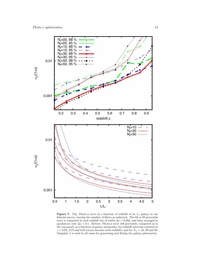
Photo-z optimizaton 14
0.001
0.01
0.2 0.3 0.4 0.5 0.6 0.7 0.8 0.9
!z/(
1+z)
redshift z
Nf=05, 68 %Nf=05, 95 %Nf=10, 68 %Nf=10, 95 %Nf=30, 68 %Nf=30, 95 %Nf=50, 68 %Nf=50, 95 %
0.001
0.01
0.5 1 1.5 2 2.5 3 3.5 4 4.5 5
!z/(
1+z)
L/L*
Nf=10Nf=30Nf=50
Figure 7. Top: Photo-z error as a function of redshift of an L∗ galaxy in ourfiducial survey, varying the number of filters as indicated. The 68 or 95 percentileerror is computed in each redshift bin of width ∆z = 0.002, and then averaged inquadrature over ∆z = 0.1. Bottom: Photo-z error (68 percentile, computed as inthe top panel) as a function of galaxy luminosity, for redshift intervals centered atz = 0.65, 0.75 and 0.85 (errors increase with redshift), and for Nf = 10, 30 and 50.Template 1 is used in all cases for generating and fitting the galaxy photometry.
Photo-z optimizaton 15
practically independent of the number of filters in our fiducial survey. At z > 0.4,there is only a small improvement of σz when Nf is increased from 10 to 30, andeven this small improvement is offset by an increasing fraction of outliers as Nf isincreased. This implies that it would not be worth to use more than ∼ 10 filters tomeasure photometric redshifts for galaxies of luminosities near L∗ that are well fittedby a single template.
The target accuracy of 0.003(1 + z) to measure radial BAO is achieved up toz ∼ 0.7 for L = L∗. The bottom panel shows that at z = 0.9 the same target can beachieved for L > 1.6L∗. For galaxies of high luminosity, increasing Nf from 10 to 30becomes a stronger advantage, but gains for Nf > 30 are not substantial, especiallybecause the outliers increase with Nf . The approximately constant redshift accuracywith the number of filters is roughly a consequence of the analytic arguments discussedin §5.1 for the case when the main spectral feature is an unresolved break. Note thatthere are also numerous features in the spectrum of template 1 (Figure 2) that canbe modelled as absorption lines of width ∼ λ/30 (particularly at wavelengths justblueward of the Hα break), which are the principal reason for the improvement ofredshift errors from Nf = 10 to Nf = 30 for high signal-to-noise.
So far, the results have been shown averaged over redshift bins of ∆z = 0.1. Theunbinned results are shown in Figure 8, for the cases Nf = 10 and Nf = 50. Thereare periodic oscillations in the redshift error, with a spacing δz that corresponds tothe separation between filters. These oscillations are due to different features in thespectrum (mostly the Hα break) crossing the center and the edge of filters as theredshift varies. The redshift error is best (smallest) when the Hα break is placedbetween two filters, and it is worst when it is placed at the center of one filter. Theseoscillations should naturally depend on the shape of the filter windows, as well as theform of the Hα break, and therefore the type of LRG galaxy. One should note thatthe scale of the oscillation corresponds to the BAO scale for Nf ' 30. The presenceof these artificial oscillations in the redshift error, which could vary their amplitudeover the survey area owing to variations of the seeing or other observing conditionsthat may systematically affect the photometry, needs to be properly calibrated andcorrected for in order to avoid introducing perturbations in the BAO peak of thegalaxy correlation function.
5.3. Using multiple templates
In reality LRG are not a perfectly uniform population described by a single spectrum.We now see the impact on the redshift errors when variations in the galaxy spectraare allowed for. We use the five templates described in §3, which have been optimizedto provide a good representation of observed galaxy spectra [20, 22].
Figure 9 shows the photo-z error for spectra generated with template 1 andL = L∗. The thin lines are the same as those shown in Figure 7 (top panel), fittedwith the same template 1. The thick lines are the result obtained when any linearcombination of the five templates is allowed in the fit. As expected, the errors increasewhen we allow for spectral variability: the maximum photo-z accuracy for an idealgalaxy having exactly the same spectrum as template 1 is obtained when we knowthat the galaxy has the spectrum of template 1. When we do not know this, andspectral variability needs to be allowed for, the photo-z error is larger. When fittingwith our five templates, the target accuracy of σz = 0.003(1 + z) is achieved only forz < 0.63 at L = L∗ for Nf = 30 (which is roughly the ideal number of filters). Results
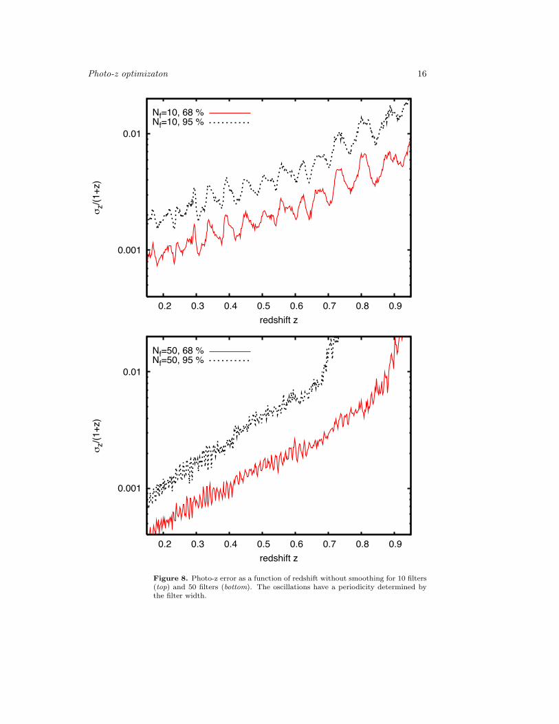
Photo-z optimizaton 16
0.001
0.01
0.2 0.3 0.4 0.5 0.6 0.7 0.8 0.9
!z/(
1+
z)
redshift z
Nf=10, 68 %Nf=10, 95 %
0.001
0.01
0.2 0.3 0.4 0.5 0.6 0.7 0.8 0.9
!z/(
1+z)
redshift z
Nf=50, 68 %Nf=50, 95 %
Figure 8. Photo-z error as a function of redshift without smoothing for 10 filters(top) and 50 filters (bottom). The oscillations have a periodicity determined bythe filter width.
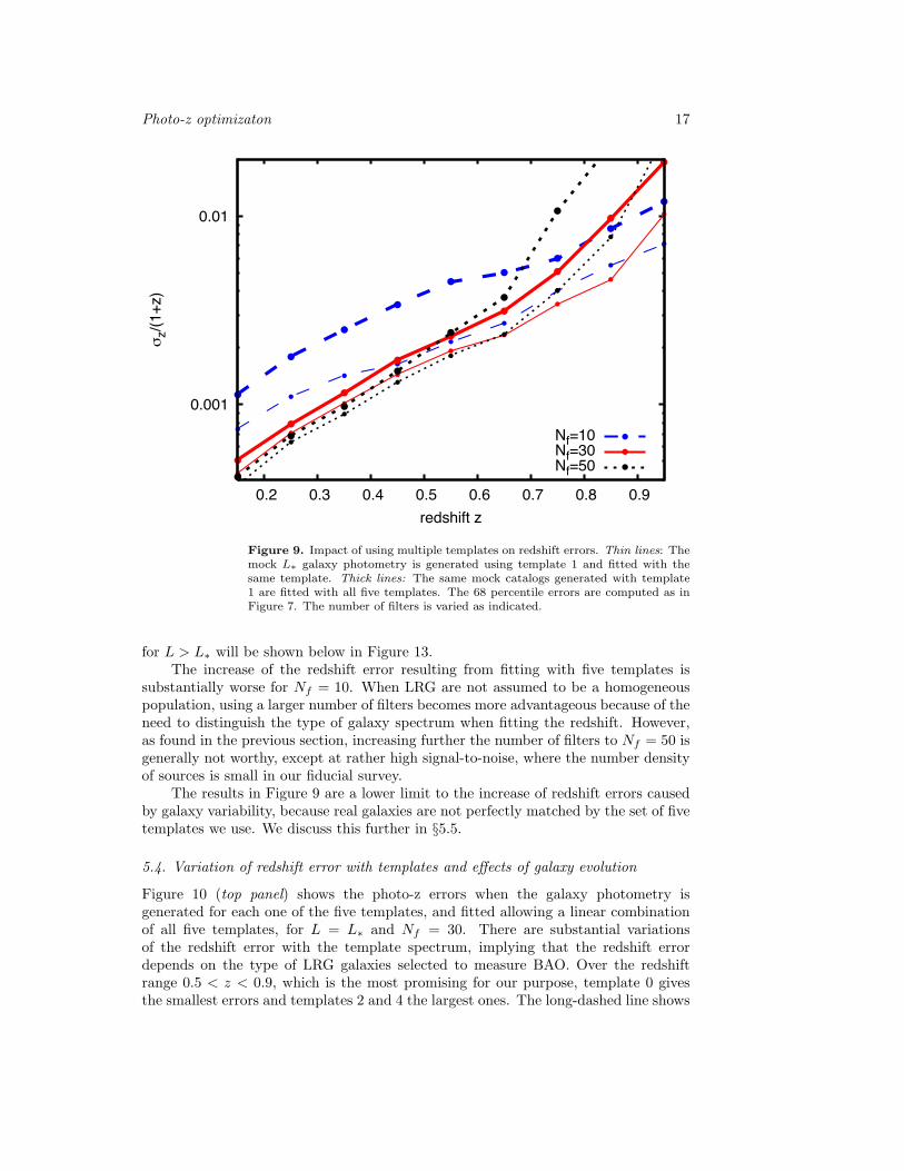
Photo-z optimizaton 17
0.001
0.01
0.2 0.3 0.4 0.5 0.6 0.7 0.8 0.9
!z/(
1+z)
redshift z
Nf=10Nf=30Nf=50
Figure 9. Impact of using multiple templates on redshift errors. Thin lines: Themock L∗ galaxy photometry is generated using template 1 and fitted with thesame template. Thick lines: The same mock catalogs generated with template1 are fitted with all five templates. The 68 percentile errors are computed as inFigure 7. The number of filters is varied as indicated.
for L > L∗ will be shown below in Figure 13.The increase of the redshift error resulting from fitting with five templates is
substantially worse for Nf = 10. When LRG are not assumed to be a homogeneouspopulation, using a larger number of filters becomes more advantageous because of theneed to distinguish the type of galaxy spectrum when fitting the redshift. However,as found in the previous section, increasing further the number of filters to Nf = 50 isgenerally not worthy, except at rather high signal-to-noise, where the number densityof sources is small in our fiducial survey.
The results in Figure 9 are a lower limit to the increase of redshift errors causedby galaxy variability, because real galaxies are not perfectly matched by the set of fivetemplates we use. We discuss this further in §5.5.
5.4. Variation of redshift error with templates and effects of galaxy evolution
Figure 10 (top panel) shows the photo-z errors when the galaxy photometry isgenerated for each one of the five templates, and fitted allowing a linear combinationof all five templates, for L = L∗ and Nf = 30. There are substantial variationsof the redshift error with the template spectrum, implying that the redshift errordepends on the type of LRG galaxies selected to measure BAO. Over the redshiftrange 0.5 < z < 0.9, which is the most promising for our purpose, template 0 givesthe smallest errors and templates 2 and 4 the largest ones. The long-dashed line shows
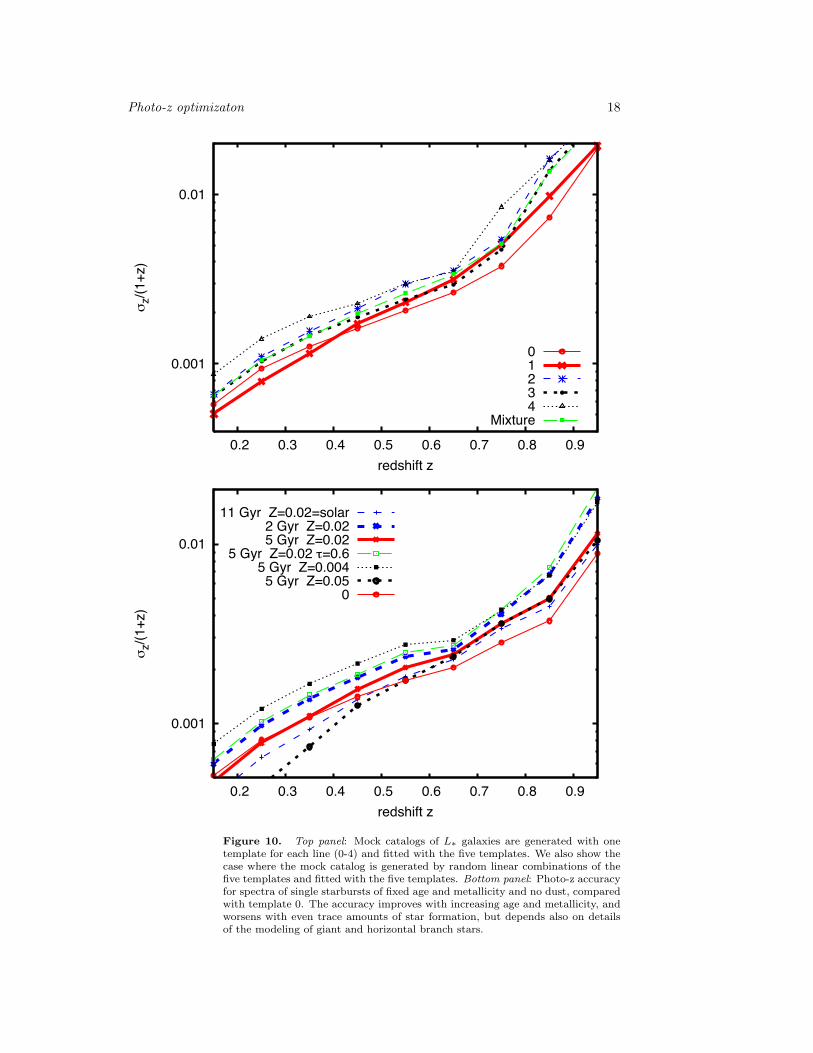
Photo-z optimizaton 18
0.001
0.01
0.2 0.3 0.4 0.5 0.6 0.7 0.8 0.9
!z/(
1+z)
redshift z
01234
Mixture
0.001
0.01
0.2 0.3 0.4 0.5 0.6 0.7 0.8 0.9
!z/(
1+z)
redshift z
11 Gyr Z=0.02=solar2 Gyr Z=0.025 Gyr Z=0.02
5 Gyr Z=0.02 "=0.65 Gyr Z=0.004
5 Gyr Z=0.050
Figure 10. Top panel: Mock catalogs of L∗ galaxies are generated with onetemplate for each line (0-4) and fitted with the five templates. We also show thecase where the mock catalog is generated by random linear combinations of thefive templates and fitted with the five templates. Bottom panel: Photo-z accuracyfor spectra of single starbursts of fixed age and metallicity and no dust, comparedwith template 0. The accuracy improves with increasing age and metallicity, andworsens with even trace amounts of star formation, but depends also on detailsof the modeling of giant and horizontal branch stars.
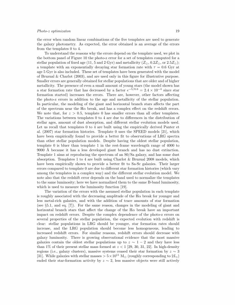
Photo-z optimizaton 19
the error when random linear combinations of the five templates are used to generatethe galaxy photometry. As expected, the error obtained is an average of the errorsfrom the templates 0 to 4.
To understand the reasons why the errors depend on the template used, we plot inthe bottom panel of Figure 10 the photo-z error for a set of templates computed for astellar population of fixed age (11, 5 and 2 Gyr) and metallicity (Z, 0.2Z, or 2.5Z);a template with an exponentially decaying star formation rate with τ = 0.6 Gyr atage 5 Gyr is also included. These set of templates have been generated with the modelof Bruzual & Charlot (2003), and are used only in this figure for illustrative purpose.Smaller errors are generally obtained for stellar populations that are older and of highermetallicity. The presence of even a small amount of young stars (the model shown hasa star formation rate that has decreased by a factor e−5/0.6 = 2.4 × 10⁻⁴ since starformation started) increases the errors. There are, however, other factors affectingthe photo-z errors in addition to the age and metallicity of the stellar population.In particular, the modeling of the giant and horizontal branch stars affects the partof the spectrum near the Hα break, and has a complex effect on the redshift errors.We note that, for z > 0.5, template 0 has smaller errors than all other templates.The variations between templates 0 to 4 are due to differences in the distribution ofstellar ages, amount of dust absorption, and different stellar evolution models used.Let us recall that templates 0 to 4 are built using the empirically derived Panter etal. (2007) star formation histories. Template 0 uses the SPEED models [21], whichhave been empirically found to provide a better fit to observations of LRG spectrathan other stellar population models. Despite having the oldest stellar population,template 0 is bluer than template 1 in the rest-frame wavelength range of 4000 to9000 A because it has a less developed giant branch and has no dust extinction.Template 1 aims at reproducing the spectrum of an S0/Sa galaxy, and has some dustabsorption. Templates 1 to 4 are built using Charlot & Bruzual 2008 models, whichhave been empirically shown to provide a better fit to Sa-Sc galaxies. Their largererrors compared to template 0 are due to different star formation histories (which varyamong the templates in a complex way) and the different stellar evolution model. Wenote also that the redshift error depends on the band used to normalize the templatesto the same luminosity; here we have normalized them to the same B-band luminosity,which is used to measure the luminosity function [19].
The variation of the errors with the assumed stellar population in each templateis roughly associated with the decreasing amplitude of the Hα break for younger andless metal-rich galaxies, and with the addition of trace amounts of star formation(see §5.1, and eq. [7]). For the same reason, changes in the modeling of giant andhorizontal branch stars that affect the change of the Hα break have an importantimpact on redshift errors. Despite the complex dependence of the photo-z errors onseveral properties of the stellar population, the expected evolution with redshift isclear: stellar populations in LRG should be younger, star formation rates shouldincrease, and the LRG population should become less homogeneous, leading toincreased redshift errors. For similar reasons, redshift errors should decrease withgalaxy luminosity. There is growing observational evidence that the most massivegalaxies contain the oldest stellar populations up to z ∼ 1 − 2 and they have lessthan 1% of their present stellar mass formed at z < 1 [29, 30, 31, 22]. In high-densityregions (i.e., galaxy clusters), massive systems ceased their star formation by z ∼ 3[31]. While galaxies with stellar masses > 5×10¹¹ M (roughly corresponding to 2L∗)ended their star-formation activity by z ∼ 2, less massive objects were still actively
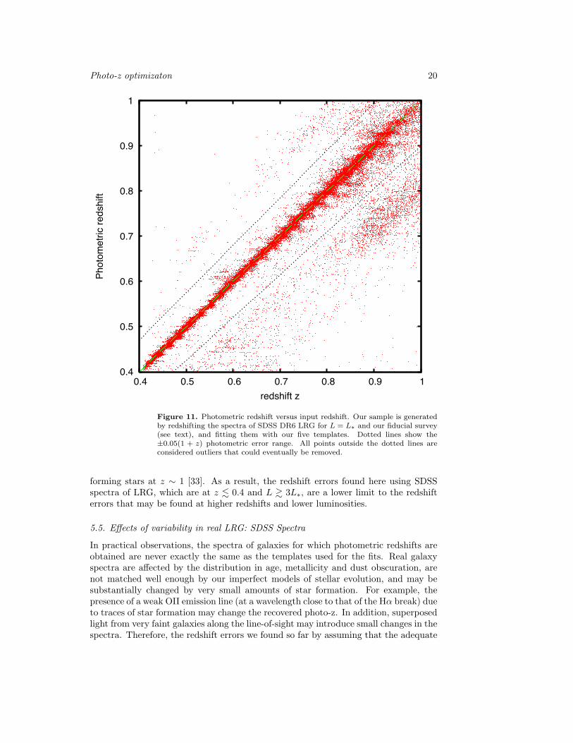
Photo-z optimizaton 20
0.4
0.5
0.6
0.7
0.8
0.9
1
0.4 0.5 0.6 0.7 0.8 0.9 1
Phot
omet
ric re
dshi
ft
redshift z
Figure 11. Photometric redshift versus input redshift. Our sample is generatedby redshifting the spectra of SDSS DR6 LRG for L = L∗ and our fiducial survey(see text), and fitting them with our five templates. Dotted lines show the±0.05(1 + z) photometric error range. All points outside the dotted lines areconsidered outliers that could eventually be removed.
forming stars at z ∼ 1 [33]. As a result, the redshift errors found here using SDSSspectra of LRG, which are at z . 0.4 and L & 3L∗, are a lower limit to the redshifterrors that may be found at higher redshifts and lower luminosities.
5.5. Effects of variability in real LRG: SDSS Spectra
In practical observations, the spectra of galaxies for which photometric redshifts areobtained are never exactly the same as the templates used for the fits. Real galaxyspectra are affected by the distribution in age, metallicity and dust obscuration, arenot matched well enough by our imperfect models of stellar evolution, and may besubstantially changed by very small amounts of star formation. For example, thepresence of a weak OII emission line (at a wavelength close to that of the Hα break) dueto traces of star formation may change the recovered photo-z. In addition, superposedlight from very faint galaxies along the line-of-sight may introduce small changes in thespectra. Therefore, the redshift errors we found so far by assuming that the adequate
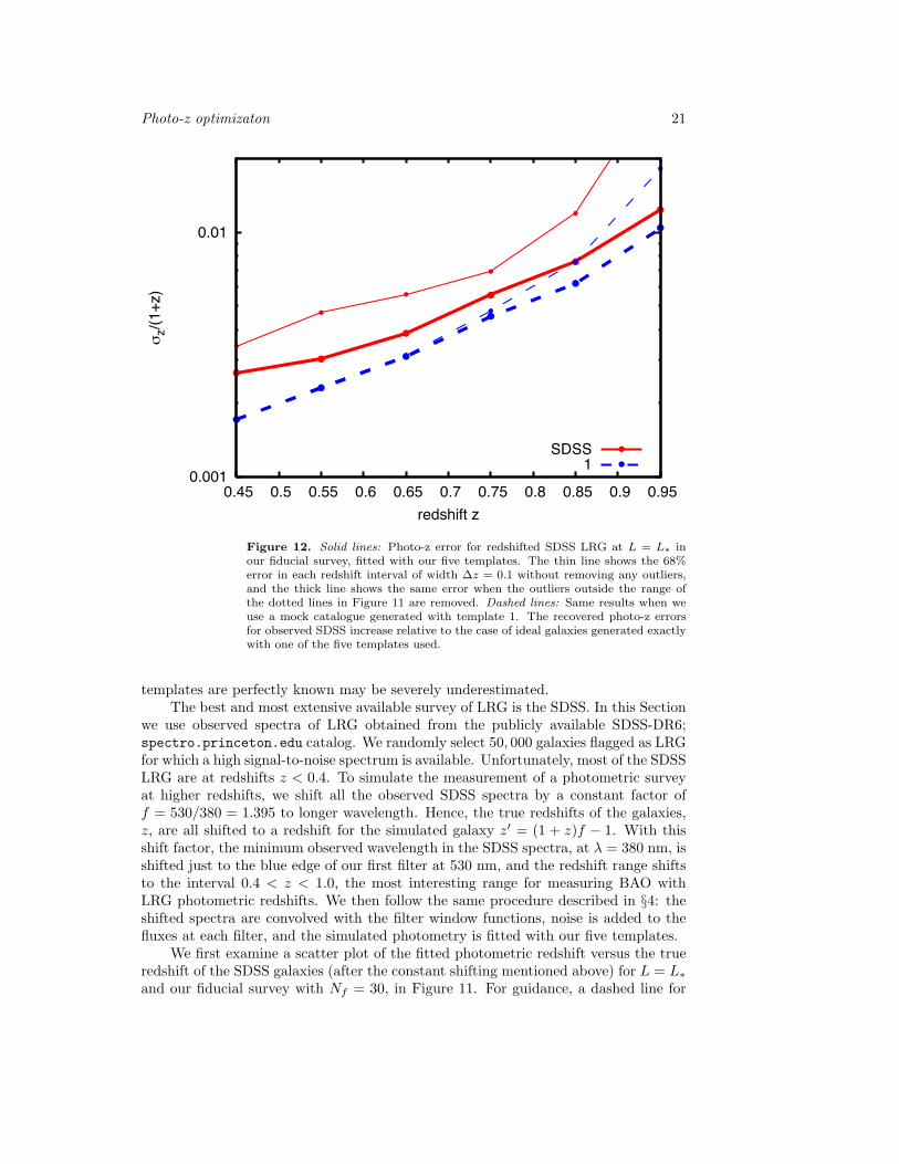
Photo-z optimizaton 21
0.001
0.01
0.45 0.5 0.55 0.6 0.65 0.7 0.75 0.8 0.85 0.9 0.95
!z/(
1+z)
redshift z
SDSS1
Figure 12. Solid lines: Photo-z error for redshifted SDSS LRG at L = L∗ inour fiducial survey, fitted with our five templates. The thin line shows the 68%error in each redshift interval of width ∆z = 0.1 without removing any outliers,and the thick line shows the same error when the outliers outside the range ofthe dotted lines in Figure 11 are removed. Dashed lines: Same results when weuse a mock catalogue generated with template 1. The recovered photo-z errorsfor observed SDSS increase relative to the case of ideal galaxies generated exactlywith one of the five templates used.
templates are perfectly known may be severely underestimated.The best and most extensive available survey of LRG is the SDSS. In this Section
we use observed spectra of LRG obtained from the publicly available SDSS-DR6;spectro.princeton.edu catalog. We randomly select 50, 000 galaxies flagged as LRGfor which a high signal-to-noise spectrum is available. Unfortunately, most of the SDSSLRG are at redshifts z < 0.4. To simulate the measurement of a photometric surveyat higher redshifts, we shift all the observed SDSS spectra by a constant factor off = 530/380 = 1.395 to longer wavelength. Hence, the true redshifts of the galaxies,z, are all shifted to a redshift for the simulated galaxy z′ = (1 + z)f − 1. With thisshift factor, the minimum observed wavelength in the SDSS spectra, at λ = 380 nm, isshifted just to the blue edge of our first filter at 530 nm, and the redshift range shiftsto the interval 0.4 < z < 1.0, the most interesting range for measuring BAO withLRG photometric redshifts. We then follow the same procedure described in §4: theshifted spectra are convolved with the filter window functions, noise is added to thefluxes at each filter, and the simulated photometry is fitted with our five templates.
We first examine a scatter plot of the fitted photometric redshift versus the trueredshift of the SDSS galaxies (after the constant shifting mentioned above) for L = L∗and our fiducial survey with Nf = 30, in Figure 11. For guidance, a dashed line for
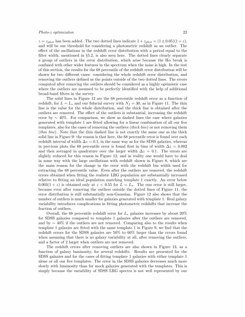
Photo-z optimizaton 22
z = zphot has been added. The two dotted lines indicate 1 + zphot = (1± 0.05)(1 + z),and will be our threshold for considering a photometric redshift as an outlier. Theeffect of the oscillations in the redshift error distribution with a period equal to thefilter width, mentioned in §5.2, is also seen here. The dotted lines clearly separatea group of outliers in the error distribution, which arise because the Hα break isconfused with other wider features in the spectrum when the noise is high. In the restof this section, the results for the 68 percentile of the redshift error distribution will beshown for two different cases: considering the whole redshift error distribution, andremoving the outliers defined as the points outside of the two dotted lines. The errorscomputed after removing the outliers should be considered as a highly optimistic casewhere the outliers are assumed to be perfectly identified with the help of additionalbroad-band filters in the survey.
The solid lines in Figure 12 are the 68 percentile redshift error as a function ofredshift, for L = L∗ and our fiducial survey with Nf = 30, as in Figure 11. The thinline is the value for the whole distribution, and the thick line is obtained after theoutliers are removed. The effect of the outliers is substantial, increasing the redshifterror by ∼ 40%. For comparison, we show as dashed lines the case where galaxiesgenerated with template 1 are fitted allowing for a linear combination of all our fivetemplates, also for the cases of removing the outliers (thick line) or not removing them(thin line). Note that the thin dashed line is not exactly the same one as the thicksolid line in Figure 9: the reason is that here, the 68 percentile error is found over eachredshift interval of width ∆z = 0.1, in the same way as for the SDSS galaxies, whereasin previous plots the 68 percentile error is found first in bins of width ∆z = 0.002and then averaged in quadrature over the larger width ∆z = 0.1. The errors areslightly reduced for this reason in Figure 12, and in reality one would have to dealin some way with the large oscillations with redshift shown in Figure 8, which arethe main reason for the change in the error with the redshift bin width used forextracting the 68 percentile value. Even after the outliers are removed, the redshifterrors obtained when fitting the realistic LRG population are substantially increasedrelative to fitting an ideal population matching template 1 exactly. An error below0.003(1 + z) is obtained only at z < 0.55 for L = L∗. The rms error is still larger,because even after removing the outliers outside the dotted lines of Figure 11, theerror distribution is still substantially non-Gaussian. Figure 12 also shows that thenumber of outliers is much smaller for galaxies generated with template 1. Real galaxyvariability introduces complications in fitting photometric redshifts that increase thefraction of outliers.
Overall, the 68 percentile redshift error for L∗ galaxies increases by about 20%for SDSS galaxies compared to template 1 galaxies after the outliers are removed,and by ∼ 40% if the outliers are not removed. Comparing also to the results whentemplate 1 galaxies are fitted with the same template 1 in Figure 9, we find that theredshift errors for the SDSS galaxies are 50% to 60% larger than the errors foundwhen assuming that there is no galaxy variability at all, after removing the outliers,and a factor of 2 larger when outliers are not removed.
The redshift errors after removing outliers are also shown in Figure 13, as afunction of galaxy luminosity, for several redshifts. Results are presented for theSDSS galaxies and for the cases of fitting template 1 galaxies with either template 1alone or all our five templates. The error in the SDSS galaxies decreases much moreslowly with luminosity than for mock galaxies generated with the templates. This issimply because the variability of SDSS LRG spectra is not well represented by our

Photo-z optimizaton 23
0.001
0.01
0.5 1 1.5 2 2.5 3 3.5 4 4.5 5
!z/(
1+z)
L/L*
SDSS vs all1 vs 1
1 vs all
Figure 13. Photo-z error as a function of luminosity. Solid lines: RedshiftedSDSS DR6 galaxies are fitted with our five templates. Dashed lines: Same resultswhen galaxies are generated with template 1, and fitted with five templates.Dotted lines: Same results for galaxies generated with template 1 and fittedwith the same template. The redshift error is the 68 percentile of the averageddistribution over each redshift interval of width ∆z = 0.1, centered at z = 0.65,0.75 and 0.85 (errors increase with redshift).
templates. For L & 2L∗, the errors for the SDSS galaxies are nearly twice as large asthe errors obtained from galaxies that match template 1 exactly, while the errors whenfitting with one or all five templates become nearly equal. The fraction of outliers isalso found to be much larger for the SDSS galaxies. The galaxy variability in theSDSS LRG is highly complex and cannot be easily accounted for with a small numberof templates, even when these templates have been calibrated with observed galaxies.
We have checked the dependence of the redshift errors on the signal-to-noisereached in the photometry. For Nf = 30, we find that the photo-z error versus thesignal-to-noise in the reddest filter (S/Nlast) is quite robust to the various assumptionsmade about the survey design. The target accuracy of σlz = 0.003 is reached for SDSSgalaxies at S/Nlast ' 20, and at S/Nlast ' 12 in the one template anlaysis. The photo-z error and the fraction of outliers increase rapidly for lower signal-to-noise. At highersignal-to-noise, the errors continue to decrease rapidly for galaxies generated with thetemplates, but they flatten out to an ”error-floor” of about σlz = 0.002 for the SDSSgalaxies, the “knee” being at around S/Nlast ∼ 30, indicating an intrinsic galaxyvariability that is not adequately modelled by a small number of templates.
A possible problem when using the SDSS spectra of LRG to model photometrymight arise from spectroscopic calibration errors, which could result in artificialvariations of the simulated fluxes that are not due to real galaxy variability but
Photo-z optimizaton 24
to calibration errors. In fact, [16] argued that SDSS spectra cannot be used tomodel variability for this reason; we reach a different conclusion. Even thoughthe spectroscopic calibration errors are found to be typically at the level of ∼ 4%on wavelength scales of 100 nm when comparing photometry and spectroscopy ofstars (see http://www.sdss.org/dr6/products/spectra/spectrophotometry.html ), theprecision of the photometric redshifts depends on measuring spectral features at thesmallest wavelength scale allowed by the narrow-band filters (for LRG, this is mostlythe Hα break). For a filter width of 10nm, the derived photometric redshifts mightbe affected by spectroscopic calibration errors on a similar wavelength scale. At thisscale, the calibration errors are much smaller: they are certainly less than 2% fromthe analysis of quasar spectra in regions with no Lyα forest absorption (P. McDonald,private communication; see also Figure 19 in [32], where the contribution to the fluxvariance due to calibration errors from different scales in quasar spectra is shownas a ratio to the Lyα forest power), and they should be less than 1% from themost recent calibration made with low-metallicity F-subdwarfs (D. Schlegel, privatecommunication). We therefore conclude that the variations in the SDSS spectra ofLRG galaxies which result in increased photometric redshift errors are mostly real andnot due to spectroscopic calibration errors.
We emphasize that, owing to galaxy evolution, the variability present in theSDSS spectra is a lower limit for the variability that should be expected for LRG athigher redshift, as discussed in §5.4. The errors might possibly be reduced by furtheroptimization of the templates as a function of galaxy luminosity and environment ifgalaxy variability at high redshift were better understood, but how substantial animprovement may be achievable in this way remains to be proven.
6. Discussion
This paper has presented an analysis of the expected photometric redshift errors inLRG that can be achieved in an imaging survey with a system of a large number ofnarrow-band filters. We have found that an optimal choice for the number of filtersis Nf ' 30 over the wavelength range 530 to 830 nm, allowing redshift measurementsover the range 0.5 < z < 0.9. A central focus of our investigation is that the intrinsicvariability of LRG implies a substantial increase of the redshift errors compared toa calculation where all the LRG are assumed to match exactly the same templateused to fit their photometry. We find that it is crucial to properly include the effectsof spectral variability when evaluating the prospects for any survey to measure BAO(particularly in the radial direction) in the power spectrum of LRG.
The implications of our results can be summarized by considering, for anyparticular survey, the lowest luminosity that a galaxy needs to have to yield a redshiftaccuracy better than the target level for measuring BAO in the radial direction,σlz < 0.003. The power of a survey to reach the required photometric accuracydepends mainly on the product Et of the etendue times the total observing time.This lowest luminosity as a function of Et is shown in the upper panel of Figure 14, atfive different redshift intervals, when the total survey area is fixed to Ω = 8000 squaredegrees and Nf = 30, for the SDSS galaxies after removing outliers with redshift errors∆z > 0.05(1+z). Note that the minimum luminosity shown at each value of Et is theone that would yield a 68 percentile error equal to σlz = 0.003; the rms error would belarger because even after removing the most extreme outliers, the error distributionis still substantially non-Gaussian. The luminosity function [19] implies the number
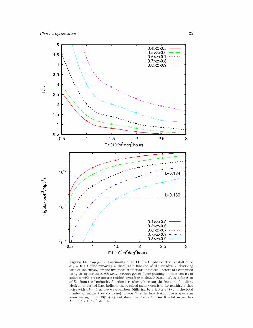
Photo-z optimizaton 25
0.5
1
1.5
2
2.5
3
3.5
4
4.5
5
0.5 1 1.5 2 2.5 3
L/L *
E!t (105m2deg2hour)
0.4>z>0.50.5>z>0.60.6>z>0.70.7>z>0.80.8>z>0.9
10-5
10-4
10-3
0.5 1 1.5 2 2.5 3
n (g
alax
ies!
h3 /Mpc
3 )
E!t (105m2deg2hour)
k=0.164
k=0.130
0.4>z>0.50.5>z>0.60.6>z>0.70.7>z>0.80.8>z>0.9
Figure 14. Top panel: Luminosity of an LRG with photometric redshift errorσlz = 0.003 after removing outliers, as a function of the etendue × observingtime of the survey, for the five redshift intervals indicated. Errors are computedusing the spectra of SDSS LRG. Bottom panel: Corresponding number density ofgalaxies with a photometric redshift error better than 0.003(1 + z), as a functionof Et, from the luminosity function [19] after taking out the fraction of outliers.Horizontal dashed lines indicate the required galaxy densities for reaching a shotnoise with nP = 1 at two wavenumbers (differing by a factor of two in the totalnumber of modes they comprise), where P is the line-of-sight power spectrumassuming σlz = 0.003(1 + z) and shown in Figure 1. Our fiducial survey hasEt = 1.5× 10⁵ m2 deg2 hr.
Photo-z optimizaton 26
density of galaxies above this minimum luminosity that is shown in the bottom panel,after subtracting outliers. As shown in Figure 1, the photometric redshift errorssuppress the power spectrum near the line-of-sight, which must be compensated by anincreased number density of galaxies to keep shot noise sub-dominant on a given scale.The bottom panel of Figure 14 addresses this issue. For redshift errors σlz = 0.003,the two horizontal dashed lines show the galaxy number density required to reducethe shot noise to the level nP = 1 at wavenumbers k = 0.13 h Mpc−1 and k = 0.164h Mpc−1 near the line-of-sight. Modes up to k = 0.164 h Mpc−1 must be sampledto fully measure the second BAO. Figure 14 shows that Et > 3 × 10⁵ m2 deg2 hris required to reach nP = 1 up to z = 0.85 for k = 0.164 h Mpc−1 near the line-of-sight. For the characteristic total observing time of 5000 hours assumed in our fiducialsurvey, this corresponds to E > 60 m2 deg2.
This minimum value for Et depends on several technical details of the telescope-camera system and the observing conditions for the survey. The assumptions madehere for our fiducial survey were specified in §4: a seeing of 0.8”, read-out noiseof 7 × 3 electrons per pixel (with a pixel size of 0.4”), the efficiency for the latestavailable CCD’s, optical losses of two mirror reflections only, and the sky brightnessof the Paranal observatory at an airmass of 1.2. These assumptions can be consideredas highly optimistic, except perhaps the assumption on the read-out noise which mightbe improved with the best available technology. Changes in these assumptions implycorresponding changes in the required value of Et necessary to reach a fixed signal-to-noise in the galaxy photometry. We can quantify this in the following way:
• A seeing degradation from 0.8” to 1.2” implies a 20% decrease in the signal-to-noise for a fixed aperture, and therefore requires a 40% increase in Et(d lnEt/d ln seeing′′ ' 1)• An increase by half a magnitude of the sky brightness (comparable for example
to the sky variation over a sun cycle or between ecliptic plane and ecliptic pole)can be compensated by a increase in Et of a factor 1.6 (d lnEt/dBsky ' 0.9)• A reduction in readout noise of a factor of three can be compensated by a ∼ 20%
reduction in Et ( d lnEt/d lnNreadout = 0.3; we have verified this by repeating allthe above calculations for a lower read-out noise). An even lower read-out noise,however, would not yield the same fractional improvement because at that pointthe read-out noise becomes subdominant.
• Any factors that decrease the overall throughput of the system (i.e., lowerefficiency of the CCD’s, additional optical losses in the telescope-camera system,reduced filter transmission, etc.) will of course increase the required Et inproportion to the inverse of the throughput. An important factor that may causesuch a reduction in the throughput would likely be present in a system of narrowfilters based on interferometry, where the filter window has a variation across thefield-of-view caused by the varying incidence angle of the light. The averagingof the filter window shape as a source moves across the field in drift-scanningmode would widen the filter window without increasing the number of detectedphotons.
These considerations mean that, in practice, the required etendue would likely besubstantially larger.
Photo-z optimizaton 27
7. Conclusions
The principal objective of this paper is to examine the potential for narrow-bandphotometric surveys to measure the radial BAO signal in the LRG power spectrum.We have revisited this issue after [12, 11, 14], addressing the optimization of thenumber of filters and filter width, discussing the dependence on the spectra ofthe target population of LRG, and considering the signal-to-noise that could berealistically achieved in a survey. We have found it to be particularly important totake into account the spectral variability of a realistic galaxy population for properlyevaluating the photometric redshift accuracy that can be achieved. Our conclusionscan be summarized as follows:
a) In agreement with [12, 11, 14] the photometric approach, even if it can achievethe target photo-z error of 0.3%, will be advantegeous only if it can cover a muchlarger fraction of the sky, with a higher galaxy density and reach higher redshiftsthan the spectroscopic surveys currently under way. Not only one needs higher sourcedensity in a photometric survey to measure the oscillations up to k ∼ 0.2, but alsothe distribution of redshift errors needs to be known accurately to correct for theireffect on the power spectrum shape and be able to measure the BAO shape. This isequivalent to the requirement of obtaining photo-z with better than 0.3% accuracyto fainter magnitudes than spectroscopy. We have concentrated on the LRG galaxiesbecause they are a fairly homogeneous population, the form of their spectra makesthem particularly suitable for good photo-z determinations and because they representthe target of choice for z < 2 BAO surveys.
b) If LRG were a perfectly homogeneous population (with spectra closely matchedby a single spectral template), the photometric redshift accuracy would not improvevery much beyond a total number of filters Nf ' 10, except for galaxies at highsignal-to-noise which would have a low number density in a survey with Et '1.5 × 10⁵ m2 deg2 hr. In reality, galaxy spectra are variable and the ideal numberof filters is Nf ' 30 over a wavelength range 530 nm < λ < 830 nm, focusing onthe redshift range 0.5 < z < 0.9. Medium-to-narrow band filters photometric redshifterrors show periodic oscillations with a spacing δz that corresponds to the filter widths.For a filter width of ∼ 100A, the scale of the oscillation corresponds to the BAO scale.The presence of these oscillations may introduce significant biases in the measurementof the BAO scale (see Section 5.2).
c) The variability of realistic galaxy spectra demand high resolution (or morefilters in a photometric survey) and high signal-to-noise. We have quantified, withrealistic simulations of a photometric survey, the minimum galaxy luminosity andthe corresponding number density for which 0.3% photo-z error can be obtained as afunction of the survey Etendue× exposure time Et (see Figure 14). We estimate theminimum value of Et necessary to measure the full second baryonic acoustic oscillationin the power spectrum, at k < 0.164 h/Mpc near the line-of-sight, with shot noisenP > 1 and up to z = 0.85, at Et ' 3× 10⁵ m2 deg2 hr. The actual required value ofEt would likely be larger when taking into account that our assumptions for the seeingand the overall throughput of the telescope-camera system are optimistic, and thatthe presence of outliers, optimistically clipped and ignored, will degrade the estimatedperformance. Moreover, the true level of galaxy variability should likely be higher thanin the SDSS LRG sample we have used (which is for z . 0.4 and L & 3L∗), becausethe variability of LRG spectra is expected to increase with redshift and decrease withluminosity.
Photo-z optimizaton 28
Current spectroscopic surveys (e.g., SDSSIII–BOSS) are obtaining spectra of themassive (> 2L∗) population of LRG at z < 0.75 to measure radial and tangentialBAO scale. Here we have investigated the conditions necessary to obtain the requiredphoto-z accuracy of 0.3% from a similar or fainter population using photometry, whichin principle is less expensive in terms of observing. We have concluded that an etendueof 30 m2 deg2 is required for tracing the same population as BOSS (z < 0.75, L > 2L∗)with radial BAO signal degraded only by ∼ 60% due to photo-z errors. But to improveon this i.e., to reach L∗ galaxies at slightly higher redshifts, the minimum etenduerequired is 60 m2 deg2 for a 5-year survey (corresponding to a 4m telescope with thelargest fields of view that have been made), and probably needs to be larger givenour optimistic assumptions we have made for the seeing, throughput, observing time,removal of outliers and systematic errors.
In this paper we have restricted our attention to the objective of measuring radialBAO with LRG. However, a large-area imaging optical survey with a large number ofnarrower bands than existing surveys would have many other applications, and mightlead to a large number of interesting astronomical discoveries. We have shown in thispaper that, for realistically achievable values of Et at the present time, the density ofLRG sources that could be measured with a narrow-band photometric survey with thetarget redshift accuracy for radial BAO will not be large enough to make it competitivewith a spectroscopic survey. Therefore, a photometric survey with a large number ofoptical narrow-bands needs to find its scientific justification in other astronomicalapplications.
Acknowledgements
We warmly thank D. Eisenstein, J. Gunn, P. McDonald and D. Schlegel for discussions.This work was carried out in the framework of the PAU Consolider Collaboration: theauthors are part of the Physics of the Accelerating Universe (PAU) proposal, currentlysupported by the Spanish Ministry for Science and Innovation (MICINN) through theConsolider Ingenio-2010 program project CSD2007-00060. DR acknowledges supportfrom the Spanish MICINN through a FPU grant. LV acknowledges the support ofFP7-PEOPLE-2002IRG4-4-IRG#202182 and CSIC I3 #200750I034. The work of RJis supported by grants from the Spanish MICINN and the European Union (FP7). JMis supported by the Spanish MICINN grants AYA2006-06341 and AYA-15623-C02-01and the European Union FP6 grant IRG-046435. CPG acknowledges MICINN grantNo. FPA2007-60323.
References
[1] Simon J., et al., 2005, PhRvD, 71, 123001[2] Komatsu E., et al., 2008, arXiv:0803.0547[3] Polarski D., Ranquet A., 2005, PhysLettB, 627, 1[4] Huang Z.Y., Wang B., Su R. K., 2007, Int J.Mod.Phys. A 22, 1819[5] Clarckson C., Cortes M., Bassett B., 2008, JCAP 0780 011[6] Baremboin G., Fernandez-Martinez E., Mena O., Verde L., in preparation.[7] Eisenstein D. J., et al., 2005, ApJ, 633, 560[8] Cole S., et al., 2005, MNRAS, 362, 505[9] Percival W., et al. 2007a, MNRAS, 381, 1053
[10] Percival, W., et al. 2007b, ApJ, 657, 645[11] Seo, H.-J., & Eisenstein, D. J. 2007, ApJ, 665, 14[12] Seo H.-J., Eisenstein D. J., 2003, ApJ, 598, 720
Photo-z optimizaton 29
[13] Wolf C., Meisenheimer K., Rix H.-W., Borch A., Dye S., Kleinheinrich M., 2003, A&A, 401, 73[14] Blake C., Bridle S., 2005, MNRAS, 363, 1329[15] Dahlen, T., et al., 2008, AJ, 136, 1361[16] Benitez N., et al., 2008, arXiv:0807.0535[17] McDonald, P., & Eisenstein, D. J. 2007, PRD, 76, 063009[18] Kaiser, N. 1987, MNRAS, 227, 1[19] Brown M. J. I., et al., 2007, ApJ, 654, 858[20] Niemack M. D., et al.., 2008, arXiv:0803.3221[21] Jimenez R., et al., 2004, MNRAS, 349, 240[22] Panter, B., et al., 2007, MNRAS, 378, 1550[23] Shen, S., et al., 2003, MNRAS, 343, 978[24] Bruzual G., Charlot S., 2003, MNRAS, 344, 1000[25] Patat, F. 2008, A&A, 481, 575[26] Roy A. E., Clarke D., 2003, Astronomy, IoP Publishing[27] BARR Associates, 2008, private communication[28] Fabricius M. H., et al., 2006, SPIE6068.[29] Cowie, L. L., Songaila, A., & Barger, A. J. 1999, AJ, 118, 603[30] Heavens A., et al., 2004, Nature, 428, 625[31] Thomas D., et al., 2005, ApJ, 621, 673[32] McDonald, P., et al. 2006, ApJS, 163, 80[33] Treu T. et al., 2005, ApJ, 633, 174
Copyright © 2022 FDOKUMEN

