


Bahasa
Halaman
Hukum


Optimal Control of Commercial Office Battery Systems, and Grid IntegratedEnergy Resources on Distribution Networks
by
Michael Derin Sankur
A dissertation submitted in partial satisfaction of the
requirements for the degree of
Doctor of Philosophy
in
Engineering - Mechanical Engineering
in the
Graduate Division
of the
University of California, Berkeley
Committee in charge:
Professor Dave Auslander, ChairProfessor Kameshwar Poolla
Assistant Professor Scott MouraAdjunct Professor Alexandra Von Meier
Fall 2017

Optimal Control of Commercial Office Battery Systems, and Grid IntegratedEnergy Resources on Distribution Networks
Copyright 2017by
Michael Derin Sankur
1
Abstract
Optimal Control of Commercial Office Battery Systems, and Grid Integrated EnergyResources on Distribution Networks
by
Michael Derin Sankur
Doctor of Philosophy in Engineering - Mechanical Engineering
University of California, Berkeley
Professor Dave Auslander, Chair
The proliferation of new sensing and actuation technologies presents new opportunitiesfor enhanced supervision, optimization, and control of energy systems. In the commercialoffice environment, the use of smart power strips, uninterruptible power supplies, and ad-vanced building energy management systems is growing as a means to implement control ofenergy efficiency measures and demand response. In electricity distribution networks, phasormeasurement units and inverters are enabling utility operators to monitor and manage dis-tribution systems more effectively. The physics or operational constraints of systems withinthe commercial office environment or distribution networks are often nonlinear or noncon-vex, and thus difficult to incorporate into optimization programs. This dissertation presentsresearch into modeling and optimal control of two nonlinear energy systems.
At the commercial office scale, we discuss the development and implementation of optimalcontrol of plug loads and office scale battery storage. Building upon successes in optimalcontrol of plug loads, we propose a model predictive controller (MPC) for the incorporationof battery storage. We derive a model of an off the shelf battery storage system throughexperimental data, and discuss extensions to allow controllable charging. We investigate twomethods to solve the nonlinear and binary MPC, and simulations show the promise dynamicprogramming method.
At the distribution network scale, we discuss power flow models for optimization of griddistributed energy resources (DER), and techniques for solving nonlinear optimal powerflow (OPF) problems. First, we study semidefinite programming as a method for solvingnonlinear OPFs for control of voltage phasors. Simulation results motivate the developmentof novel models. We then derive a linearized unbalanced power flow model (LUPFM) for usein convex optimal power flow (OPF) formulations. The LUPFM builds upon previous workby adding a relationship between voltage phasor and complex power flow. A study into theLUPFM accuracy shows its fidelity for benchmark networks. We discuss two applicationsof the LUPFM. The first is balancing of voltage magnitude on a distribution network, andsimulations are successful for both radial and mesh networks. The second application is

2
minimization of voltage magnitude and angle difference for switching operations. Simulationsshow the success and potential of the LUPFM for OPF control of voltage phasors.

i
To Nellie the Elephant
See you on the road to Mandalay
ii
Contents
Contents ii
List of Figures v
List of Tables vii
1 Introduction 11.1 Modeling and Optimal Control of Commercial Office Plug Loads and Battery
Storage Systems . . . . . . . . . . . . . . . . . . . . . . . . . . . . . . . . . . 11.2 Optimization and Control of Distribution Network Scale Energy Systems . . 21.3 Research Contributions . . . . . . . . . . . . . . . . . . . . . . . . . . . . . . 31.4 Organization of this Dissertation . . . . . . . . . . . . . . . . . . . . . . . . 4
I Modeling and Optimal Control of Commercial Office PlugLoads and Battery Storage Systems 5
2 Introduction 6
3 Model Predictive Control of Plug Loads and an Office Scale BatteryStorage System 8
4 Experimentally Derived OSBS Battery Model 14
5 An Exhaustive Search Numerical Method and Simulation Results 195.1 Exhaustive Search Numerical Method . . . . . . . . . . . . . . . . . . . . . . 195.2 Simulation Results using Exhaustive Search Method . . . . . . . . . . . . . . 21
6 A Dynamic Programming Algorithm for the MPC Optimization Pro-gram and Simulation Results 306.1 Dynamic Programming Algorithm . . . . . . . . . . . . . . . . . . . . . . . . 306.2 Simulation Results using Dynamic Programming Algorithm . . . . . . . . . 32
iii
7 Concluding Remarks and Future Work 39
II Modeling of Unbalanced Power Flow and Optimal Controlof Distributed Energy Resources for Grid Reconfiguration 41
8 Introduction 428.1 Nomenclature, Definitions, and Preliminaries . . . . . . . . . . . . . . . . . . 44
9 A Discussion of Semidefinite Programming for Optimal Power FlowProblems 499.1 Introduction . . . . . . . . . . . . . . . . . . . . . . . . . . . . . . . . . . . . 499.2 Previous Research in SDP for OPFs . . . . . . . . . . . . . . . . . . . . . . . 509.3 Extensions of the SDP OPF for Control of Voltage Phasors . . . . . . . . . . 529.4 Conclusions . . . . . . . . . . . . . . . . . . . . . . . . . . . . . . . . . . . . 62
10 Derivation of a Linearized Unbalanced Power Flow Model 6410.1 Introduction . . . . . . . . . . . . . . . . . . . . . . . . . . . . . . . . . . . . 6410.2 Derivation of Power and Losses for Unbalanced Approximate Power Flow . . 6510.3 Derivation of Voltage Magnitude Relations for Unbalanced Approximate Power
Flow . . . . . . . . . . . . . . . . . . . . . . . . . . . . . . . . . . . . . . . . 6710.4 Derivation of Voltage Angle Relations for Unbalanced Approximate Power Flow 7110.5 Linearized Unbalanced Power Flow Model . . . . . . . . . . . . . . . . . . . 75
11 Accuracy Analysis of Linearized Unbalanced Power Flow Approximation 77
12 Applications of the Linearized Unbalanced Power Flow Model 8312.1 Voltage Magnitude Balancing . . . . . . . . . . . . . . . . . . . . . . . . . . 8312.2 Phasor Difference Minimization for Switching Operations . . . . . . . . . . . 90
13 Concluding Remarks and Future Work 99
14 Conclusion 10114.1 Modeling and Optimal Control of Commercial Office Plug Loads and Battery
Storage Systems . . . . . . . . . . . . . . . . . . . . . . . . . . . . . . . . . . 10114.2 Modeling of Unbalanced Power Flow and Optimal Control of Distributed En-
ergy Resources for Grid Reconfiguration . . . . . . . . . . . . . . . . . . . . 102
Bibliography 103
A Distribution Network Parameters 108A.1 Parameters of the Five Node Network . . . . . . . . . . . . . . . . . . . . . . 108A.2 Parameters of the IEEE 13 Node Test Feeder . . . . . . . . . . . . . . . . . 109

iv
A.3 Parameters of the Nine Node Meshed Network . . . . . . . . . . . . . . . . . 112
B Newton-Raphson Algorithm for Solving Approximate Unbalanced PowerFlow 117
C Derivation of a Half-space Approximations for L2 Norm Constraints 121
v
List of Figures
3.1 Office plug loads and OSBS presided over by an EIG . . . . . . . . . . . . . . . 103.2 Plot of inconvenience function r(Qt) where Qr = 40 and rr = 0.1. . . . . . . . . 13
4.1 APC UPS charging cycle SOC and net power. . . . . . . . . . . . . . . . . . . . 154.2 APC UPS computed charging power and piecewise linear charging power model. 17
5.1 Demand response (DR) and load-following (LF) scenario load-shed targets. . . . 225.2 Total and component load-shed of plug loads and an OSBS for static target scenario. 235.3 Demand response scenario simulation results for UPS and CBS. . . . . . . . . . 285.4 Load-following scenario simulation results for UPS and CBS. . . . . . . . . . . . 29
6.1 OSBS operation states for DR scenario. . . . . . . . . . . . . . . . . . . . . . . . 356.2 Performance comparison between UPS and CBS for DR scenario. . . . . . . . . 366.3 OSBS operation states for LF scenario. . . . . . . . . . . . . . . . . . . . . . . . 376.4 Performance comparison between UPS and CBS for LF scenario. . . . . . . . . . 38
8.1 Simple network showing node voltages, line currents, and line impedances . . . . 468.2 Diagram of simple network showing node voltage, node load, line impedance, and
line complex power. . . . . . . . . . . . . . . . . . . . . . . . . . . . . . . . . . . 46
9.1 Diagram of simple network used in SDP OPF Simulations. . . . . . . . . . . . . 549.2 Results of OPF (9.16) simulations with varying voltage magnitude reference and
reactive power dispatch penalty. Blue dots represent cases with rank-one solu-tions. Red dots represent cases where a rank-one solution was not obtained. . . 57
9.3 Results of OPF (9.16) simulations with varying voltage magnitude reference andreactive power dispatch penalty. Blue dots represent cases with rank-one solu-tions. Red dots represent cases where a rank-one solution was not obtained. . . 57
11.1 IEEE 13 node feeder topology modified for accuracy analysis of unbalanced ap-proximate power flow model. . . . . . . . . . . . . . . . . . . . . . . . . . . . . . 79
11.2 Maximum voltage magnitude error across all phases and nodes from Monte Carlosimulation. . . . . . . . . . . . . . . . . . . . . . . . . . . . . . . . . . . . . . . 80
11.3 Apparent power error from Monte Carlo simulation. . . . . . . . . . . . . . . . . 80

vi
11.4 Monte Carlo simulation results for voltage angle error and total vector error forcase where all voltage magnitudes are assumed to be 1 in (10.44). . . . . . . . . 81
11.5 Monte Carlo simulation results for voltage angle error and total vector error forcase where voltage magnitudes in (10.44) are assigned to the values from solvingpower flow. . . . . . . . . . . . . . . . . . . . . . . . . . . . . . . . . . . . . . . 82
12.1 Modified IEEE 13 node feeder topology for voltage magnitude balancing simulation. 8512.2 Plot of voltage magnitudes for base case of voltage magnitude balancing scenario 8612.3 Plot of voltage magnitudes for control case of voltage magnitude balancing scenario 8612.4 Comparison of voltage magnitude imbalance for voltage balancing scenario. . . . 8712.5 Nine node mesh network topology. . . . . . . . . . . . . . . . . . . . . . . . . . 8812.6 Plot of voltage magnitudes for base case of voltage magnitude balancing scenario
for nine node mesh network . . . . . . . . . . . . . . . . . . . . . . . . . . . . . 8812.7 Plot of voltage magnitudes for control case of voltage magnitude balancing sce-
nario for nine node mesh network . . . . . . . . . . . . . . . . . . . . . . . . . . 8912.8 Comparison of voltage magnitude imbalance for voltage balancing scenario for
nine node mesh network. . . . . . . . . . . . . . . . . . . . . . . . . . . . . . . . 8912.9 Distribution network composed of two IEEE 13 node feeder models connected to
same transmission line. . . . . . . . . . . . . . . . . . . . . . . . . . . . . . . . . 92
C.1 Tangential half-space approximation of circle. . . . . . . . . . . . . . . . . . . . 123C.2 Error of half-space approximation of apparent power constraint. . . . . . . . . . 123

vii
List of Tables
3.1 Nomenclature for Part I. . . . . . . . . . . . . . . . . . . . . . . . . . . . . . . . 93.2 OSBS decision variables and operation states. . . . . . . . . . . . . . . . . . . . 11
5.1 Plug loads used in simulations. . . . . . . . . . . . . . . . . . . . . . . . . . . . 225.2 Comparison of UPS and CBS performance for DR scenario. . . . . . . . . . . . 255.3 Comparison of UPS and CBS performance for LF scenario. . . . . . . . . . . . . 27
6.1 OSBS control states in Figure 6.1 and Figure 6.3. . . . . . . . . . . . . . . . . . 33
8.1 Nomenclature for Part II. . . . . . . . . . . . . . . . . . . . . . . . . . . . . . . 45
9.1 Voltage from solving power flow [48] with zero DER dispatch. . . . . . . . . . . 55
12.1 Optimal DER dispatch for voltage balancing on IEEE 13 node feeder . . . . . . 8712.2 Optimal DER dispatch for voltage balancing on nine node mesh network . . . . 9012.3 Results of phasor matching for switching action simulation. . . . . . . . . . . . . 9512.4 Optimal DER dispatch for phasor matching and switching action . . . . . . . . 9612.5 Results of phasor matching for switching action simulation. . . . . . . . . . . . . 9712.6 Optimal DER dispatch for phasor matching and switching action . . . . . . . . 98
A.1 Five node network node parameters . . . . . . . . . . . . . . . . . . . . . . . . . 108A.2 Five node network line parameters. . . . . . . . . . . . . . . . . . . . . . . . . . 108A.3 Five node network complex demands . . . . . . . . . . . . . . . . . . . . . . . . 109A.4 Five node network capacitors . . . . . . . . . . . . . . . . . . . . . . . . . . . . 109A.5 Five node network DER apparent power capacity. . . . . . . . . . . . . . . . . . 109A.6 IEEE 13 node test network node phases . . . . . . . . . . . . . . . . . . . . . . 109A.7 IEEE 13 node test network line parameters. . . . . . . . . . . . . . . . . . . . . 111A.8 IEEE 13 node test feeder complex demands . . . . . . . . . . . . . . . . . . . . 112A.9 IEEE 13 node test feeder capacitors . . . . . . . . . . . . . . . . . . . . . . . . . 112A.10 IEEE 13 node feeder DER apparent power capacity . . . . . . . . . . . . . . . . 112A.11 Nine node mesh network node parameters . . . . . . . . . . . . . . . . . . . . . 113A.12 Nine node mesh network line parameters. . . . . . . . . . . . . . . . . . . . . . . 115A.13 Nine node mesh network complex demands . . . . . . . . . . . . . . . . . . . . 116

viii
A.14 Nine node mesh network capacitors . . . . . . . . . . . . . . . . . . . . . . . . . 116A.15 Nine node mesh network DER apparent power capacity. . . . . . . . . . . . . . 116

ix
Acknowledgments
First and foremost, I would like to thank my advisor Professor Dave Auslander for all thehelp, advice, insight, and support that he has given me during my time as Ph.D. student. Igrateful for the opportunity to work with him, and all of the knowledge and experience thatI have gained from being his student.
I owe a large debt of gratitude to my friend, colleague, and mentor Dr. Dan Arnold.His continued friendship, support, and guidance has helped me immensely throughout thisprocess. I am very grateful to have worked alongside Dan, and without him this dissertationwould not be possible.
I want to express my deep gratitude to Professor Alexandra Von Meier for her supportand mentorship. Her research insight and feedback have been invaluable. I also want tothank her for the opportunity to be a graduate student instructor.
I would like to thank Professor Kameshwar Poolla for serving on my dissertation commit-tee. I also want to thank Professor Scott Moura for serving on my dissertation committee,for his dissertation feedback and advise, and for the opportunity to be a graduate studentinstructor.
I am grateful to Professors Karl Hedrick, Dennis Lieu, Shmuel Oren, and KameshwarPoolla for serving on my qualification exam committee.
I would like to thank the Department of Defense and the National Defense Science andEngineering Graduate Fellowship program, for the award in 2009.
I want to express my gratitude to my colleagues from the DIADR (A Distributed In-telligent Automated Demand Response Building Management System, # DE-EE0003847)project: Tyler Jones, Andrew Krioukov, Nate Murthy, Jorge Ortiz, Therese Peffer, JayTaneja, Jason Trager, Rongxin Yin, Siyuan Zhou, and the research staff at Siemens.
I want to thank my colleagues from the OpenBAS (Open Building Automation System,#DE-EE0006351) project: Therese Peffer, Marco Pritoni and Jacob Cabrera.
I want to thank my colleagues from the ARPA-E (#DE-AR0000340) project: Kyle Bradyand Roel Dobbe.
I am grateful to Emma Stewart for providing employment and research opportunities atLawrence Berkeley National Laboratory.
I want to thank my family. My mother Vega and father Haluk have provided tremendoussupport and inspiration with unlimited patience throughout this process. I am grateful to mysister Ailene as she was my childhood role model and she inspired me to seek an education.I am also grateful she did not earn a PhD, as I have now won this round of sibling rivalry.
I am very grateful for my family friend Marla Petal for her invaluable help in motivationand organization.

1
Chapter 1
Introduction
With the advent of new technologies ranging from smart power strips, uninterruptiblepower supplies, the internet of things, advanced metering infrastructure for electric grid,micro synchophasor measurement units, to inverters there are new and exciting areas inwhich to apply optimization and control theory to energy systems. However, many of thesesystems have nonlinear physics or nonlinear operational characteristics and thus requiresuitable mathematical models or optimization techniques. The focus of this work is toapply modeling, optimization and control techniques to two nonlinear energy systems. Thefirst system is a commercial office with plug loads and battery storage. The second is anunbalanced distribution network with integrated distributed energy resources (DER).
1.1 Modeling and Optimal Control of Commercial
Office Plug Loads and Battery Storage Systems
Commercial buildings are becoming increasingly metered and controllable with the adop-tion of technologies such as smart meters, smart power strips, and advanced building energymanagement systems [19, 49]. Economic incentives such as time-of-use electricity pricing hasled to many research efforts in and the advancement of technologies for commercial buildingefficiency and demand response.
An area often overlooked until recently in commercial buildings for load-shedding areplug loads [3, 19, 40]. Systems such as office scale battery storage (OSBS) are enabling peakload reduction and load shifting actions to be complemented by plug loads [41]. In this work,we study the modeling optimal control of plug loads and an OSBS in a commercial officesetting. The effort is detailed in Part I of this dissertation.
This work builds upon previous effort of plug load control [2, 4, 3, 40], we focus mainlyon the integration of an off the shelf OSBS system. Firstly, a model predictive controller(MPC) is formulated that encapsulates the behavior or plug loads. A battery charging anddischarging model is derived from experimental data. The battery model is nonlinear andnonconvex, with two modes of operation. Next, techniques for obtaining the optimal control
CHAPTER 1. INTRODUCTION 2
state of plug loads and the OSBS are discussed. The first technique is an exhaustive searchalgorithm, and simulations highlight its shortcomings. The second technique studied isdynamic programming. Simulations show its strength in optimizing over long time horizonswith good time granularity.
1.2 Optimization and Control of Distribution
Network Scale Energy Systems
Modeling, formulation, and solving of optimal power flow (OPF) problems is an areaof research that is increasingly important with the advent of renewable and distributedenergy resources, and the increasing ubiquity of grid sensors and data [43]. An importantarea for the application of OPF is grid reconfiguration for grid stability, reliability andintegration of micro-gridding. In this work, we study OPFs that seek to manage DER forgrid reconfiguration actions on an unbalanced network.
The physics of power flow are nonlinear and nonconvex, making it difficult to directlyincorporate the physics into an reliably and easily solvable OPF problem. To address this,research has focused on semidefinite programming (SDP) and approximate power flow models[7], however literature has highlighted some drawbacks that may preclude its widespreadapplicability [24, 27]. Novel linearized models for unbalanced power flow are used for theirlinear properties, however their approximate nature may not capture important nonlinearphysics [14, 39].
Our first effort in this area is to develop SDP OPFs for control of voltage magnitude andangle, and to explore convergence to a physically meaningful solution through simulation.We propose and derive several OPFs for control of voltage phasors. Simulations motivatefurther study in the control of voltage magnitude, and show the viability of placing boundson voltage angle.
Our second effort is to develop a model that can be incorporated into a convex pro-gram, and thus we derive a linearized unbalanced power flow model (LUPFM). This modelaugments previous literature [14, 39] by adding a relationship for voltage angle and com-plex power flow. We investigate the accuracy of the LUPFM, and find it acceptable forbenchmark networks.
Two OPF applications of the LUPFM are discussed. The first OPF seeks to balancevoltage magnitude across different phases at nodes on a network. Simulation results showthe ability of the OPF to reduce voltage imbalance for both radial and mesh networks.The second OPF seeks to minimize the voltage phasor difference between two points on anetwork for switching actions. Simulation results show the ability of the OPF to regulatevoltage magnitude and angles at different points on a network.
CHAPTER 1. INTRODUCTION 3
1.3 Research Contributions
The contributions of Part I, titled Modeling and Optimal Control of Commercial Office PlugLoads and Battery Storage Systems, of this work are as follows:
- Chapter 3: A model predictive control formulation is developed that expands on previouswork in optimal control of plug loads [3, 40]. This MPC incorporates devices commonlyfound in commercial offices and an abstract energy storage model.
- Chapter 4: A battery model of an off the shelf uninterruptible power supply (UPS) is de-rived through experimentation. To incorporate a real UPS into the MPC from Chapter 3,its battery discharging and charging and charge controller characteristics are investigatedand modeled.
- Chapter 5: An exhaustive search method for solving the MPC is investigated. Simulationresults show the limited viability of this method.
- Chapter 6: A dynamic programming method for solving the MPC is investigated. Simu-lation results show its promise as a viable method for optimizing over extended periods.
The contributions of Part II, titled Modeling of Unbalanced Power Flow and Optimal Controlof Distributed Energy Resources for Grid Reconfiguration, of this work are as follows:
- Chapter 9: The derivation and investigation of SDP OPFs for control of voltage phasors.Simulation results further motivate efforts in this area, and the exploration of other powerflow models.
- Chapter 10: The derivation of a linearized unbalanced power flow model (LUPFM). Thismodel augments that of [14, 39] by incorporating a relationship between voltage angle andcomplex power flow.
- Chapter 11: The accuracy of the LUPFM is investigated, with simulation results demon-strating model accuracy for benchmark networks.
- Chapter 12: Two OPFs that incorporate the LUPFM are designed and experiments areperformed demonstrating the its effectiveness in OPFs for voltage control.
- Section 12.1: OPF1 seeks to minimize voltage magnitude imbalance across a distributionnetwork. Simulation results show significant reduction in voltage imbalance.
- Section 12.2: OPF2 seeks to minimize voltage phasor difference (both voltage magnitudedifference and angle difference) between two points in a network for switching actions.Simulations show OPF2 controlling both voltage magnitude and angle, thus reducingpotential power flow across an open switch scheduled to be closed.

CHAPTER 1. INTRODUCTION 4
1.4 Organization of this Dissertation
Part I of this dissertation is concerned with modeling and optimal control of office scalebattery storage systems.
- Chapter 2 gives overview of existing technologies and summarizes the effort undertaken inPart I.
- Chapter 3 discusses the derivation of an MPC for optimal load-shedding through controlof plug loads and battery storage.
- Chapter 4 discusses the derivation of a battery system operation model through experi-mental data.
- Chapter 5 presents an exhaustive search control algorithm and simulation results arediscussed.
- Chapter 6 derives and discusses a dynamic programming algorithm for optimizing OSBScontrol state, and simulation results for two scenarios are discussed.
- Chapter 7 provides concluding remarks and a discussion of future work.
Part II of this dissertation is concerned with power flow models and optimization of distri-bution networks.
- Chapter 8 summarizes the current state of research into linear and nonlinear OPFs andoutlines the research effort of Part II.
- Chapter 9 discusses research in using SDP for OPF for control of voltage magnitude andangle.
- Chapter 10 provides a derivation of a linearized unbalanced power flow model.
- Chapter 11 investigates the accuracy of the LUPFM from Chapter 10.
- Chapter 12 provides discussion of two applications of the LUPFM in OPFs for voltagecontrol, and simulations.
- Chapter 13 provides concluding remarks and a discussion of future work.
Conclusions for this dissertation are drawn in Chapter 14.

5
Part I
Modeling and Optimal Control ofCommercial Office Plug Loads and
Battery Storage Systems

6
Chapter 2
Introduction
The commercial building sector accounts for 36 % of electrical energy consumption inthe United States [45]. The advent and increasing ubiquity of smart-meters, tiered andtime-of-use pricing has led to research in and advancements of commercial demand responsetechnologies. Many successful efforts in reducing building peak power, and energy consump-tion, target building HVAC and lighting systems. Building HVAC and lighting are majorconsumers of electricity. These systems are likely to be centrally controlled and metered.
Plug loads, on the other hand, are often neglected as a resource for demand response.Plug loads can account for 30 % to 50 % of energy consumption in commercial buildings [49,19]. A plug load is a device that draws electrical power from an outlet for operation. Thisincludes, but not limited to, desktop computers, desktop monitors, fans, persona, heaters,and lamps. Their inclusion as a resource for demand response would greatly increase theflexibility and efficacy of a DR system. Plug loads are usually not utilized for DR for severalreasons. The foremost reason is their distributed nature and lack of centralized point ofaccess and control. Plug loads most often lack the necessary intelligence for self-monitoringand control so intermediary devices are needed for these purposes. Finally, the cost to retrofita building with meterable and controllable outlets is often prohibitive.
Advancements in technologies are enabling plug loads to become a load-shed resourcefor DR. One such technology is the smart power strip (SPS). An SPS is a device comprisedof one or more electrical outlets. The outlets are independently metered and controllable,and enable the user to selectively power connected devices. A second enabling technologyis the Energy Information gateway (EIG). An EIG is a software system that interfaces withexisting hardware (such as an SPS) for plug load monitoring and control [2, 4, 40]. Athird enabling technology is battery storage, specifically office scale battery storage (OSBS)system. An OSBS system provides power to one or more plug loads from outlet power orfrom its own battery power. Many commercial environments contain one or more OSBSsystems for protection against power failure. The increasing adoption and ubiquity of SPSs,EIGs, and OSBS systems in commercial environments prompts the investigation of optimalcontrol of an OSBS system and plug loads as load-shedding resources.
There have been many research efforts focused on the incorporation of plug loads and
CHAPTER 2. INTRODUCTION 7
battery storage in the context of DR. The authors in [34] present a model predictive control(MPC) framework for coordinated control of laptop battery charging for DR. Their algorithmsimplifies to a modified knapsack problem with constraints to avoid over cycling betweencharging and discharging states. Their simulations show that laptop batteries are a viableresource for load-shifting. In [36] the authors present an MPC framework to reduce peakelectricity demand. The authors develop a room thermal model to account for thermalstorage and varying tariffs on electricity.
The authors in [17] develop an algorithm for optimal storage use in a demand responsecontext. They propose a simple convex optimization program that does not require pricinginformation. In [46], the authors use dynamic programming to develop control policies ofbattery storage for residential demand response. They minimize the residential energy costtaking advantage of predictions of variable pricing signals. Optimal energy storage controlpolicies are developed in [21], where the authors utilize a dynamic programming algorithm.However, many of these efforts do not address the control of battery storage in conjunctionwith plug loads, or employ simple or generalized battery models.
Much of our previous effort has focused on the development of our own EIG [2], [4], [40].EIG development was spread across several projects. The initial project was to develop anopen-source reference model of an EIG for a residential setting, sponsored by the CaliforniaEnergy Commission (CEC) and the California Institute for Energy and the Environment(CIEE). The EIG was adapted for and deployed in a commercial setting as part of a projectwith Siemens. Further development includes several iterations and the use of a linear solverfor optimal plug load control. We successfully demonstrated the EIG exercising optimal con-trol of plug loads in a commercial office during a load-following (LF) scenario, and validatedsimulation results with physical experiments [3].
In this work, we investigate optimal control of an OSBS system alongside plug loadsfor load-shedding. We look at two OSBS systems, investigating the value of controllablecharging. We develop a model predictive control (MPC) framework to account for varyingload-shed targets and OSBS battery dynamics. An experientially derived battery modelis presented. An exhaustive search numerical method is discussed, and simulation resultsdemonstrate the the use of an OSBS alongside plug loads as a load-shed resource. Simulationresults also quantify the value of controllable charging for increasing battery capacities. Adynamic programming algorithm is discussed. The algorithm produces control variable lookup tables and quantifies OSBS performance. lastly, this work is summarized and plans tocarry this work forward are discussed.
8
Chapter 3
Model Predictive Control of PlugLoads and an Office Scale BatteryStorage System
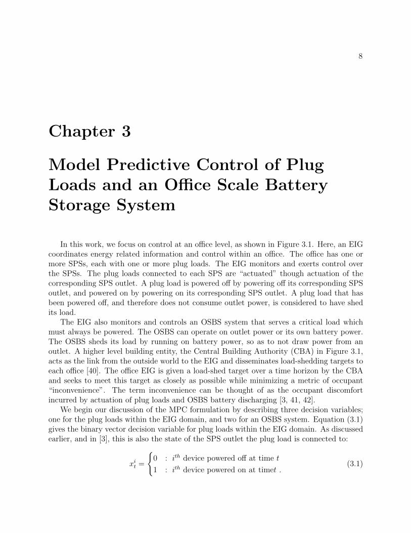
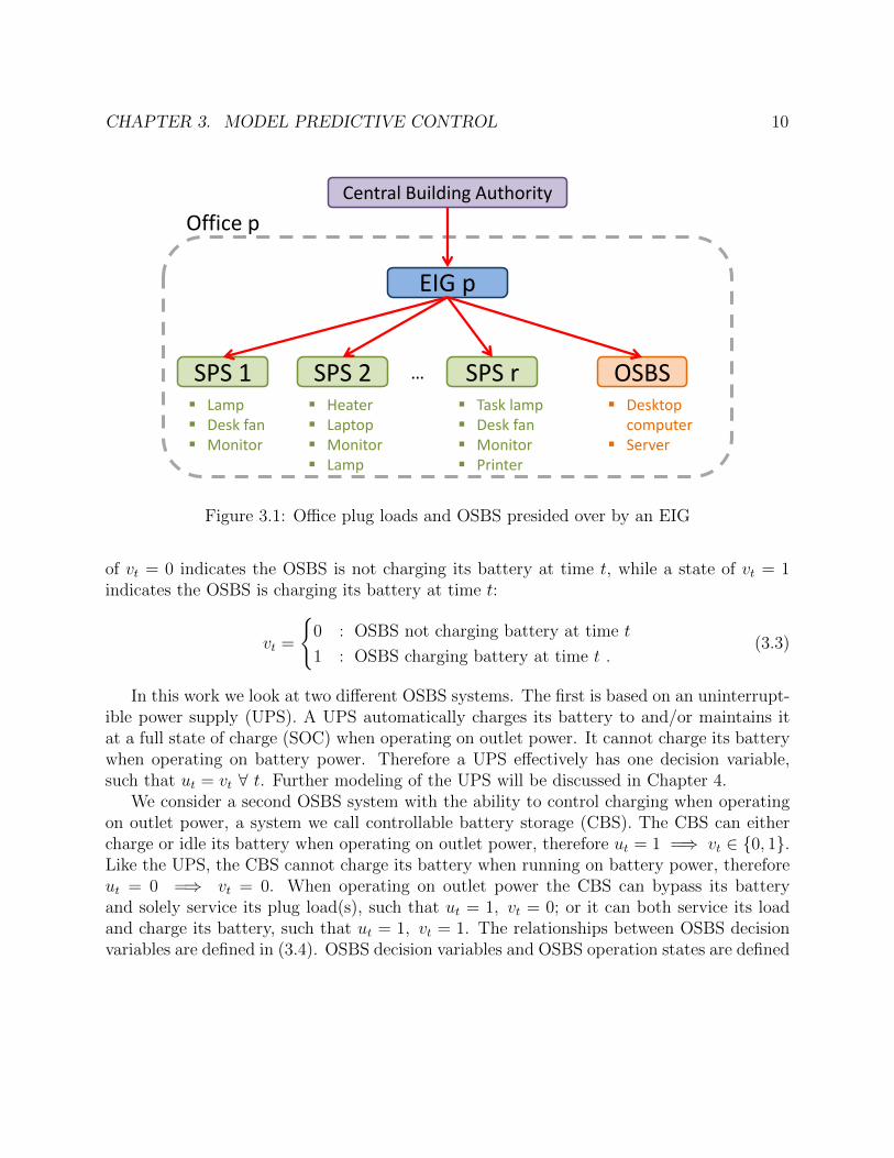
In this work, we focus on control at an office level, as shown in Figure 3.1. Here, an EIGcoordinates energy related information and control within an office. The office has one ormore SPSs, each with one or more plug loads. The EIG monitors and exerts control overthe SPSs. The plug loads connected to each SPS are “actuated” though actuation of thecorresponding SPS outlet. A plug load is powered off by powering off its corresponding SPSoutlet, and powered on by powering on its corresponding SPS outlet. A plug load that hasbeen powered off, and therefore does not consume outlet power, is considered to have shedits load.
The EIG also monitors and controls an OSBS system that serves a critical load whichmust always be powered. The OSBS can operate on outlet power or its own battery power.The OSBS sheds its load by running on battery power, so as to not draw power from anoutlet. A higher level building entity, the Central Building Authority (CBA) in Figure 3.1,acts as the link from the outside world to the EIG and disseminates load-shedding targets toeach office [40]. The office EIG is given a load-shed target over a time horizon by the CBAand seeks to meet this target as closely as possible while minimizing a metric of occupant“inconvenience”. The term inconvenience can be thought of as the occupant discomfortincurred by actuation of plug loads and OSBS battery discharging [3, 41, 42].
We begin our discussion of the MPC formulation by describing three decision variables;one for the plug loads within the EIG domain, and two for an OSBS system. Equation (3.1)gives the binary vector decision variable for plug loads within the EIG domain. As discussedearlier, and in [3], this is also the state of the SPS outlet the plug load is connected to:
xit =
{0 : ith device powered off at time t
1 : ith device powered on at timet .(3.1)

CHAPTER 3. MODEL PREDICTIVE CONTROL 9
Sym-bol
Description Unit
γt Load-shed target at time t for an office [W]
c Vector denoting power consumption of office plug loads [W]
pt Vector denoting inconveniences associated with actuation of office plugloads at time t
[-]
xt Vector of binary decision variables denoting power state of office plugloads at time t
[-]
σt Maximum allowable inconvenience associated with office plug loads attime t
[-]
LT Total load on OSBS [W]
St OSBS battery energy at time t [J]
K OSBS total battery energy capacity [J]
Qt OSBS battery state of charge (SOC), representing percent of batteryenergy St of total battery capacity K
[%]
Pt OSBS charging power at time t [W]
Pt OSBS average charging power over time t to t+ ∆T [W]
ut Binary decision variable indicating OSBS outlet power state [Z]
vt Binary decision variable indicating OSBS battery charging state [Z]
rt Inconvenience as a function of SOC at time t [-]
N Prediction horizon of model predictive control (MPC) [-]
βpl Weighting given to inconvenience of plug load actuation [W]
βsoc Weighting given to inconvenience of battery discharge [W]
Table 3.1: Nomenclature for Part I.
The binary decision variable for OSBS power, ut, is defined by (3.2). This decisionvariable refers to whether the OSBS is operating on power from its own battery, or operatingon power drawn from an outlet. A state of ut = 0 indicates the OSBS operates on its batterypower at time t. A state of ut = 1 indicates the OSBS operates on power drawn from anoutlet at time t. The term “operates” in this context refers to running the OSBS andservicing any connected plug loads:
ut =
{0 : OSBS operating on battery power at time t
1 : OSBS operating on outlet power at time t .(3.2)
The binary decision variable for OSBS charging state, vt, is defined by (3.3). A state
CHAPTER 3. MODEL PREDICTIVE CONTROL 10
EIG p
SPS 1 SPS 2 SPS r OSBS …
Lamp Desk fan Monitor
Heater Laptop Monitor Lamp
Task lamp Desk fan Monitor Printer
Desktop computer
Server
Central Building Authority
Office p
Figure 3.1: Office plug loads and OSBS presided over by an EIG
of vt = 0 indicates the OSBS is not charging its battery at time t, while a state of vt = 1indicates the OSBS is charging its battery at time t:
vt =
{0 : OSBS not charging battery at time t
1 : OSBS charging battery at time t .(3.3)
In this work we look at two different OSBS systems. The first is based on an uninterrupt-ible power supply (UPS). A UPS automatically charges its battery to and/or maintains itat a full state of charge (SOC) when operating on outlet power. It cannot charge its batterywhen operating on battery power. Therefore a UPS effectively has one decision variable,such that ut = vt ∀ t. Further modeling of the UPS will be discussed in Chapter 4.
We consider a second OSBS system with the ability to control charging when operatingon outlet power, a system we call controllable battery storage (CBS). The CBS can eithercharge or idle its battery when operating on outlet power, therefore ut = 1 =⇒ vt ∈ {0, 1}.Like the UPS, the CBS cannot charge its battery when running on battery power, thereforeut = 0 =⇒ vt = 0. When operating on outlet power the CBS can bypass its batteryand solely service its plug load(s), such that ut = 1, vt = 0; or it can both service its loadand charge its battery, such that ut = 1, vt = 1. The relationships between OSBS decisionvariables are defined in (3.4). OSBS decision variables and OSBS operation states are defined
CHAPTER 3. MODEL PREDICTIVE CONTROL 11
in Table 3.2:
UPS:ut = 0 =⇒ vt = 0
ut = 1 =⇒ vt = 1
CBS:ut = 0 =⇒ vt = 0
ut = 1 =⇒ vt ∈ {0, 1} .
(3.4)
OSBS ut vt Operation State
UPS0 0 UPS operating on battery power and not charging its battery.
1 1 UPS drawing outlet power and charging/maintaining battery to/at100% SOC.
CBS
0 0 CBS operating on battery power and not charging its battery.
1 0 CBS drawing outlet power and not charging its battery.
1 1 CBS drawing outlet power and charging/maintaining battery to/at100% SOC.
Table 3.2: OSBS decision variables and operation states.
The objective function of the MPC is given in (3.5), in which two terms are summedover a time horizon. The first term is the absolute value of the difference between the targetload-shed, and the load-shed from plug loads, cT (xt − 1), and the OSBS, LT (ut − 1) +Ptvt.The charging power is included in this term as battery charging requires drawing poweradditional to the OSBS load being serviced. It should be noted that as plug load powerand OSBS power are discrete, the load-shed target is not likely to be exactly met, and anunder-shed or over-shed will likely occur. The second term is the measure of inconvenienceor incurred by actuation of plug loads and OSBS battery discharge. In (3.5), X0→N−1 refersto the sequence of xt from t = 0 to t = N − 1. The same applies for U0→N−1 for ut andV0→N−1 for vt.
minimizeX0→N−1U0→N−1V0→N−1
N−1∑t=0
∣∣γt + cT (xt − 1) + LT (ut − 1) + Pt (Qt) vt∣∣ . . .
+ βplpTt (1− xt) + βsocrt(Qt) .
(3.5)
The generalized set of constraints of the MPC is given by (3.6). Here, (3.6a) representsbattery state of charge (SOC) dynamics in time as a function of the current SOC, the totalload on the OSBS and its operation state. Equation (3.6b) is the average charging powerover the timestep from t to t + ∆T as a function of the current SOC, rt. A measure of
CHAPTER 3. MODEL PREDICTIVE CONTROL 12
inconvenience as a function of SOC is given in (3.6c). The derivation of an OSBS model for(3.6a), (3.6b), and (3.6c) will be discussed in the subsequent section:
Qt+1 = fSOC(Qt, LT , ut, vt) ∀ t ∈ {0, N − 1} (3.6a)
Pt = fP (Qt) ∀ t ∈ {0, N − 1} (3.6b)
rt = fr(Qt) ∀ t ∈ {0, N − 1} (3.6c)
Qt ≥ Qmin,t ∀ t ∈ {0, N} (3.6d)
pTt ≤ σt (1− xt) ∀ t ∈ {0, N − 1} (3.6e)
xt ∈ χt ∀ t ∈ {0, N − 1} (3.6f)
xit ∈ {0, 1} ∀ i ∀ t ∈ {0, N − 1} (3.6g)
ut ∈ {0, 1} ∀ t ∈ {0, N − 1} (3.6h)
vt ∈ {0, 1} ∀ t ∈ {0, N − 1} . (3.6i)
A time varying minimum SOC constraint is given by (3.6d). This constraint is includedas many batteries incur damage at low SOCs, and an occupant may want to maintain aminimum SOC as a power failure safeguard. A time varying constraint on the maximumallowable inconvenience incurred from plug load actuation is given by (3.6e). This constraintrepresents the user’s desire to meet the target without incurring too much inconvenience.As in [3], this can also be considered the point at which meeting the load-shed target is nolonger as valuable to the occupant as use of their plug loads. A time of use constraint forplug loads is given by (3.6f), indicating the occupants need to use their devices at certaintimes. Equation (3.6g) enforces the binary nature of plug load operation. Finally (3.6h)and (3.6i) enforce OSBS control states as binary. Equations (3.5) and (3.6) comprise theoptimization program for the model predictive controller.
A model of the inconvenience incurred by discharging the UPS was also developed, givenby (3.7). While there is a constraint placed on the SOC (3.6), (3.7) in the objective (3.5)serves to penalize low OSBS SOC. The constraints and penalty may arise from concernsabout battery life and the desire to always maintain a minimum reserve SOC in case ofpower failure:
rt(Qt) =
1−
(1− rrQr
)Qt : 0 ≤ Qt ≤ Qr
rr
(100−Qt
100−Qr
): Qr ≤ Qt ≤ 100 .
(3.7)
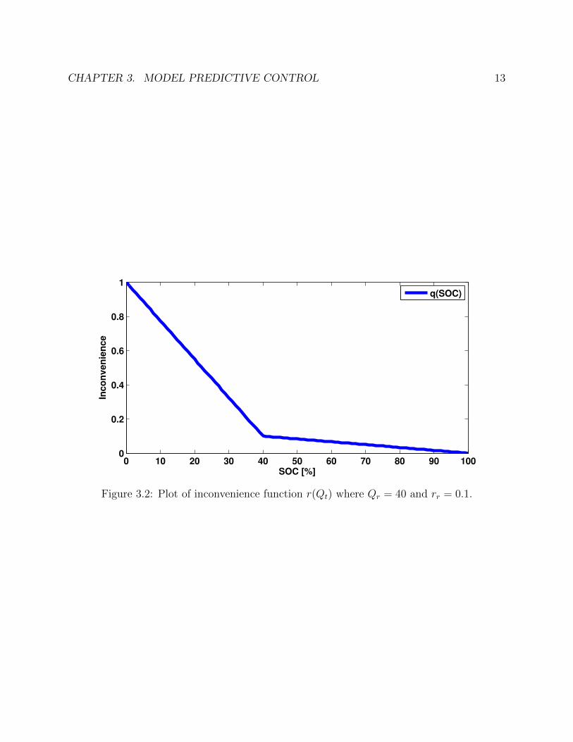
We chose a piecewise linear function, whose value remains relatively small for high SOCsand increases dramatically as the SOC decreases past a cutoff. An example of this functionwith values Qr = 40 and rr = 0.1 can be seen in Figure 3.2. The penalty function on SOCis likely to be a business decision and so will not be discussed in detail in this work.
CHAPTER 3. MODEL PREDICTIVE CONTROL 13
0 10 20 30 40 50 60 70 80 90 1000
0.2
0.4
0.6
0.8
1
SOC [%]
Inc
on
ve
nie
nc
e
q(SOC)
Figure 3.2: Plot of inconvenience function r(Qt) where Qr = 40 and rr = 0.1.
14
Chapter 4
Experimentally Derived OSBSBattery Model
A dynamic model of a commercially available OSBS was experimentally developed forthis MPC formulation. The OSBS is an uninterruptible power supply (UPS), the AmericanPower Conversion (APC) Smart UPS 1500RXLM, referred to the APC UPS. The APCUPS operates on its battery power when outlet power is disconnected, until outlet poweris restored or the battery reaches a minimum state of charge whereupon it shuts down.When outlet power is connected the APC UPS charges its battery to, and/or maintains itsbattery, at 100% SOC. The UPS model described in the previous section, and defined by(3.4) is based on the operational nature of the APC UPS. The APC UPS cannot control itscharging independently when it is drawing outlet power.
As the system state is the OSBS SOC, we seek to derive a model which captures batterycharging power as a function of battery state of charge (SOC). In order to model the APCUPS, it was discharged to several pre-defined SOCs by connecting a load and disconnectingoutlet power. After the APC UPS reached the target SOC, outlet power was restored andthe APC UPS was allowed to charge to 100% SOC. This was done for a range of connectedplug loads, including loads of 60 W, 120 W and 180 W. From the APC UPS software, time,percent (%) battery capacity, and battery voltage was recorded in one (1) minute intervals.The power drawn by the APC UPS was recorded in 15 second intervals with an SPS. Thepower drawn from the APC UPS by the connected plug load was recorded in 15 secondintervals by a second SPS. It was observed in all tests that the APC UPS drew an almostconstant amount of power additional to the connected load when not charging its battery.This was confirmed by analyzing the power data recorded by the two SPSs. The tests andpower data also showed that the connected plug load drew nearly the same amount of powerregardless APC UPS operation state, differing by 3 % at maximum.
The APC UPS percent battery capacity was assumed to be its battery SOC. As SPSpower trace data was recorded at 15 second intervals, it was linearly interpolated to fit theone minute intervals of the APC UPS data. Thus a set of SOC and power data was createdfor the APC UPS. The power drawn by the plug load was subtracted from the power drawn
CHAPTER 4. EXPERIMENTALLY DERIVED OSBS BATTERY MODEL 15
60 90 120 150 180 210 24020
40
60
80
100
Time [min]
SO
C [
%]
(a) APC UPS battery capacity (SOC) recorded during charging cycle.
60 90 120 150 180 210 2400
50
100
150
200
250
Time [min]
Net
Po
wer
[W]
(b) APC UPS net power consumption during charging cycle. This is the difference between themeasured power drawn by the UPS and that drawn by the loads connected to the UPS.
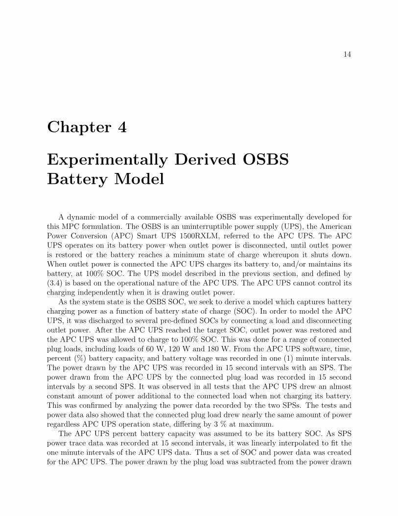
Figure 4.1: APC UPS charging cycle SOC and net power. In this figure, the black dashedline represents the switch from a period of nearly constant power draw to that of decayingpower draw. The magenta dotted line represents the time at which the SOC reaches 100%,assumed to be when charging is complete.
by the APC UPS to obtain the net power consumed by the APC UPS.Figure 4.1 shows the data for a test in which the UPS was discharged to a 20 % SOC
with a nominal load of 180 W. Figure 4.1b shows the SOC increasing in an linear fashion intime. In Figure 4.1b it can be seen that the APC UPS drew an almost constant amount ofnet power as the its SOC increased from 20 % to 50 %. The net power decreases as the SOCincreases from 50 % to 100 %. After the battery reaches, and stays at, 100 % SOC it canbe seen that the APC UPS continues to draw a decaying amount of power. As we look touse battery SOC as a state variable and parameterize charging power in SOC, it is assumedthat charging is complete once the battery has reached 100 % SOC. The time and data afterthe APC UPS reaches 100 % SOC is neglected. When the APC UPS initially reaches 100 %SOC it can be seen that it is drawing roughly 60 W net, which is assumed to be the constantUPS operation power. From these observations we arrive at a battery charging model forthe UPS, listed below:
1. Constant APC operation power during all power states of 60 W.

CHAPTER 4. EXPERIMENTALLY DERIVED OSBS BATTERY MODEL 16
2. Connected plug load draws constant power regardless of UPS power state.
3. Constant charging power when SOC between 0% and 50% of 140 W.
4. Charging completed when APC UPS reaches 100 % SOC.
We select a battery energy model in which the SOC Qt is the percent of total batteryenergy capacity at time t. Battery energy at time t is represented by St. The total batteryenergy capacity K is the maximum amount of energy the battery can hold, defined as themaximum time the OSBS can operate on battery power (discharge to zero energy) with anominal load, including operating power. Therefore the SOC Qt is defined as in (4.1):
Qt =StK× 100 % . (4.1)
As K is a constant, it is trivial to replace Qt with St in equations. The SOC dynamicsare represented as battery energy dynamics, given by (4.2), similar to the model presentedin [17]:
St+1 = St +[(ut − 1)(LT ) + ηcvtPt(St)
]∆T . (4.2)
Battery energy is linear in time, and binary in the control states ut and vt. Here, Pt denotesthe average amount of charging power over from time t to t+∆T . The variable ηc representsbattery charging efficiency, and is chosen as 1. This equation demonstrates the binary natureof the APC UPS, as it either operates on battery power or outlet power. The battery energymodel is generalized with both OSBS decision variables to be used for both the UPS andCBS model. The battery energy dynamics can also be written solely in terms of the SOCby using (4.1), resulting in the OSBS SOC dynamics, (4.3):
Qt+1 = Qt +K
100
[(ut − 1)(LT ) + ηcvtPt(St)
]∆T . (4.3)
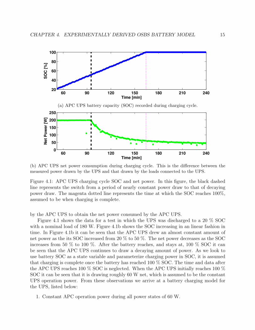
Battery charging power was parametrized in battery SOC as in (4.4). This functioncaptures the constant charging power draw from 0 to 50 % SOC, as seen in Figure 4.1.The decaying charging power seen as SOC increases from 50 to 100 % was modeled using aconstrained least squares fit. A piecewise linear function was ostensibly chosen to place theoptimization program within a linear programming framework:
Pt (Qt) =
140 : 0 ≤ Qt ≤ 50
510− 7.4Qt : 50 ≤ Qt ≤ 60
240− 2.9Qt : 60 ≤ Qt ≤ 75
90− 0.9Qt : 75 ≤ Qt ≤ 100 .
(4.4)
The piecewise linear function was constrained such that: Pt(50) = 140 to represent thetransition between constant and decaying power draw, Pt maintains piecewise continuity,and Pt(100) = 0 to represent the completion of charging at 100 % SOC. Figure 4.2 depicts
CHAPTER 4. EXPERIMENTALLY DERIVED OSBS BATTERY MODEL 17
25 40 55 70 85 1000
30
60
90
120
150
180
SOC [%]
Po
wer
[W]
Charging Power Computed
Charging Power Model
Figure 4.2: APC UPS computed charging power and piecewise linear charging power model.
the charging power model, with 3 linear segments for the decaying charging power regime.The piecewise linear function was also ostensibly selected so that the optimization programwould be compatible with a linear programming framework.
The full MPC optimization program, with the SOC as the state, is written as (4.5). Itshould be noted that this program is nonlinear, binary in its decision variables, and hasseveral switched modes from the battery charging model.

CHAPTER 4. EXPERIMENTALLY DERIVED OSBS BATTERY MODEL 18
minimizeX0→N−1U0→N−1V0→N−1
N−1∑t=0
∣∣γt + cT (xt − 1) + LT (ut − 1) + Pt (Qt) vt∣∣ . . .
+ βplpTt (1− xt) + βsocrt(Qt)
subject to ∀ t ∈ {0, N − 1}Qt+1 = Qt + (K/100)
[(ut − 1)(LT ) + ηcvtPt(St)
]∆T
Pt(Qt) =
140 : 0 ≤ Qt ≤ 50
510− 7.4Qt : 50 < Qt ≤ 60
240− 2.9Qt : 60 < Qt ≤ 75
90− 0.9Qt : 75 < Qt ≤ 100
rt(Qt) =
((Qr − 1 + rr)/Qr)Qt : 0 ≤ Qt ≤ Qr
rr(100−Qt)/(100−Qr) : Qr ≤ Qt ≤ 100
Qt ≥ Qmin,t
pTt (1− xt) ≤ σt
xt ∈ χtxit ∈ {0, 1} ∀ iut ∈ {0, 1}vt ∈ {0, 1} .
(4.5)

19
Chapter 5
An Exhaustive Search NumericalMethod and Simulation Results
5.1 Exhaustive Search Numerical Method
The full MPC optimization program is given by (3.5)-(4.4), and concisely presented in(4.5). The MPC objective function contains a binary term LTut and a nonlinear binaryterm, utPt(Qt). The non-convex piecewise linear charging power model introduces switchedmodes into the set of MPC constraints. Additionally the decision variables xt, ut, and vt areall binary. The nature of this MPC program precludes it from being solved by many popularsolvers as they are not well suited to handle these types of problems.
It is clear that the aforementioned nonlinearities and non-convexities come from thebinary nature of OSBS operation and its charging power model. By removing all termsassociated with the OSBS from (3.5) and (3.6), the optimization program is reduced to abinary integer linear program (BILP) quite similar to that in [3]. This can be leveraged tosolve the optimization program by an exhaustive search.
We denote a general sequence of ut from t = 0 to N − 1 as U0→N−1, and that of vt asV0→N−1. For any combination of U0→N−1 and V0→N−1, and Q0, the sequences S1→N andQ1→N can be calculated by (4.2). Using (4.4) the sequence P 0→N−1 can be computed, ascan r0→N−1 with (3.7). Treating these sequences as exogenous parameters, like the load-shedtarget γt, the optimization problem is reduced to an N step BILP as in(5.1):
minimizeX0→N−1
N−1∑t=0
∣∣γt + cT (xt − 1n) + (LT ) (u�t − 1) + Pt‡(Qt)v
�t
∣∣ . . .+ βplp
Tt (1n − xt) + βsocr
‡t (Qt)
subject to pTt (1n − xt) ≤ σt ∀ t ∈ {0, N − 1}xt ∈ χt ∀ t ∈ {0, N − 1}xt ∈ {0, 1} ∀ t ∈ {0, N − 1} .
(5.1)
CHAPTER 5. AN EXHAUSTIVE SEARCH NUMERICAL METHOD ANDSIMULATION RESULTS 20
Here, the superscript � denotes the decision variables from the combination of U0→N−1 andV0→N−1, and the superscript ‡ denotes the calculated values for the combination. The decisionvariable X0→N−1 is the sequence of xt for t = 0 to N − 1.
This method discretizes the portion of the state space of (3.5) and (3.6) representingthe OSBS, keeping the decision variables representing plug loads free. The simplificationremoves the nonlinearities and non-convex switched battery model from the optimizationprogram. The optimization program of (3.5) and (3.7) is reduced to a BILP (5.1) of dimen-sion nN , where n is the number of plug loads, for which many open source and commercialsolvers are available. As in (3.4), it can be seen that the UPS effectively has one decisionvariable, therefore U0→N−1 = V0→N−1. The CBS has two decision variables, thus U0→N−1and V0→N−1 may differ. Not all combinations of U0→N−1 and V0→N−1 will be feasible fromCBS operation and (3.4). The optimal decision variable sequences X∗0→N−1, U
∗0→N−1, and
V ∗0→N−1 are obtained by comparing every combination of every permutation of U0→N−1 andV0→N−1. This is done by comparing the BILP objective value for the each combination.Thus, the algorithm for solving the MPC optimization problem is as follows:
1. Grid ut and vt over all possible permutations of U0→N−1 and V0→N−1.
2. Iterate over all sequences U0→N−1 (UPS), or all combinations of sequences U0→N−1 andV0→N−1 (CBS).
- For CBS only, check feasibility of current sequence combination with regard toCBS operation, and proceed only if feasible.
3. Evolve OSBS dynamics (4.2) and (4.4) for the current decision variable sequence (UPS)or combination (CBS) over horizon t = 0 to N − 1.
4. Check feasibility of current sequence or combination with regard to minimum SOCconstraint (3.6d) over horizon t = 0 to N − 1 (UPS and CBS)
5. Solve BILP (5.1) if current sequence or combination is feasible.
6. Compare current BILP objective to best obtained thus far:
- If better, store objective, U0→N−1, V0→N−1 and X0→N−1 as best thus far.
- Otherwise, discard.
7. Return optimal solution after BILP solved for all feasible sequences (UPS) or combi-nations (CBS).
This method returns the optimal decision variable sequences for plug loads and the UPSor CBS over the time horizon t = 0 to N − 1. For a prediction horizon of N steps, thereare 2N permutations of U0→N−1. The BILP must be solved for all feasible, with regard toSOC, permutations of U0→N−1 to obtain the optimal decision variables sequences of X∗0→N−1and U∗0→N−1. The CBS has two decision variables, and therefore two sequences, there are

CHAPTER 5. AN EXHAUSTIVE SEARCH NUMERICAL METHOD ANDSIMULATION RESULTS 21
22N = 4N possible combinations of the permutations of U0→N−1 and V0→N−1. As there arethree CBS operation states, there are 3N permutations feasible with regard to CBS operation.Not all permutations will be feasible with regard to the minimum SOC constraint.
It should be noted that this method can quickly become intractable with an increasingMPC prediction horizon and/or number of OSBSs. For an office with a single UPS andprediction horizon N = 10, the algorithm would need to compare 210 possible sequences,solving the BILP of dimension 10n for each feasible sequence. For an EIG domain with mUPSs, there are 2mN possible combinations of sequence permutations. Though a powerfulcomputer may be able to handle longer prediction horizons, this method may still deliversuboptimal results. Small timesteps may cause the temporal length of the prediction horizonto be too short. The inability to predict far enough into the future may cause “shortsighted”policies to be implemented, due to load-shed target changes outside the prediction horizon.Longer timesteps would ameliorate this problem, however this would mean averaging theOSBS charging power and battery dynamics over a longer time period. The exponentialcomputational scaling associated with this method preclude both longer prediction horizonsand greater dimensionality in the number of OSBSs per EIG.
5.2 Simulation Results using Exhaustive Search
Method
We now present results from simulations of an EIG exerting control of office plug loadsand an OSBS. The simulations are for a 360 minute period with a load-shed period of 180minutes from 60 to 240 minutes. Outside the load-shed period, rule based control is appliedto the OSBS, such that the UPS and CBS charge their batteries to 100% SOC. During theload-shed period the MPC is employed to obtain the optimal decision variable sequences.The MPC optimization program is solved at each timestep setting the current timestep ast = 0. The MPC implements the first decision variable of each sequence, x∗0, u
∗0, and v∗0 for
the duration of the timestep.We consider two scenarios for simulations; a DR scenario and a load-following (LF)
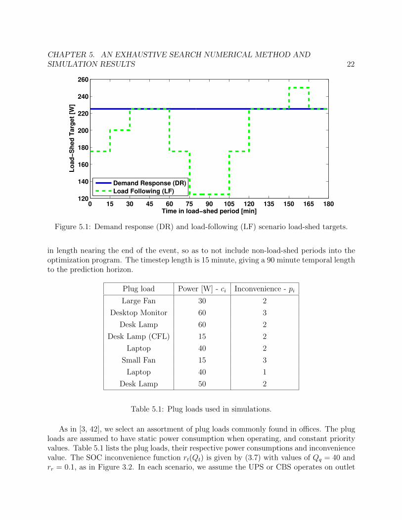
scenario. A static load-shed target is assigned by the CBA to the EIG in the DR scenario.In the LF scenario, the load-shed target is variable in time. The load-shed targets are shownin Figure 5.1. Each scenario is simulated with a range of battery capacities (run times), from60 minutes to 210 minutes in 30 minute increments. The minimum allowable SOC is 10%to allow for prolonged operation on battery power.
The UPS and CBS service a load of 120 W, and their operating power is 60 W as perthe APC UPS model. Therefore when operating on battery power their load-shed is 180 W.The plug load inconvenience weighting βpl is 10, and the SOC inconvenience weighting βsoc ischosen as 5. The maximum allowable inconvenience σt is 4 during load-shed periods, and 0otherwise. The maximum prediction horizon is chosen as N = 6 to balance the performanceof the MPC algorithm and computational expediency. The prediction horizon decreases
CHAPTER 5. AN EXHAUSTIVE SEARCH NUMERICAL METHOD ANDSIMULATION RESULTS 22
0 15 30 45 60 75 90 105 120 135 150 165 180120
140
160
180
200
220
240
260
Time in load−shed period [min]
Lo
ad
−S
he
d T
arg
et
[W]
Demand Response (DR)
Load Following (LF)
Figure 5.1: Demand response (DR) and load-following (LF) scenario load-shed targets.
in length nearing the end of the event, so as to not include non-load-shed periods into theoptimization program. The timestep length is 15 minute, giving a 90 minute temporal lengthto the prediction horizon.
Plug load Power [W] - ci Inconvenience - pi
Large Fan 30 2
Desktop Monitor 60 3
Desk Lamp 60 2
Desk Lamp (CFL) 15 2
Laptop 40 2
Small Fan 15 3
Laptop 40 1
Desk Lamp 50 2
Table 5.1: Plug loads used in simulations.
As in [3, 42], we select an assortment of plug loads commonly found in offices. The plugloads are assumed to have static power consumption when operating, and constant priorityvalues. Table 5.1 lists the plug loads, their respective power consumptions and inconveniencevalue. The SOC inconvenience function rt(Qt) is given by (3.7) with values of Qq = 40 andrr = 0.1, as in Figure 3.2. In each scenario, we assume the UPS or CBS operates on outlet
CHAPTER 5. AN EXHAUSTIVE SEARCH NUMERICAL METHOD ANDSIMULATION RESULTS 23
0 30 60 90 120 150 180 210 240 270 300 330 360−150
−100
−50
0
50
100
150
200
250
Time [min]
Lo
ad
−S
hed
[W
]
Target γt
Total Load Shed
0 30 60 90 120 150 180 210 240 270 300 330 360−150
−100
−50
0
50
100
150
200
250
Time [min]
Lo
ad
−S
hed
[W
]
Plug−Loads
UPS
(a) Load-shed from plug loads and UPS.
0 30 60 90 120 150 180 210 240 270 300 330 360−150
−100
−50
0
50
100
150
200
250
Time [min]
Lo
ad
−S
hed
[W
]
Target γt
Total Load Shed
0 30 60 90 120 150 180 210 240 270 300 330 360−150
−100
−50
0
50
100
150
200
250
Time [min]
Lo
ad
−S
hed
[W
]
Plug−Loads
CBS
(b) Load-shed from plug loads and CBS.
Figure 5.2: Total and component load-shed of plug loads and an OSBS for static targetscenario.
power and is allowed to charge before and after the load-shed period. The UPS or CBSbegin the simulation with 100 % SOC.
Model Predictive Control of Plug Loads and an OSBS forLoad-Shedding
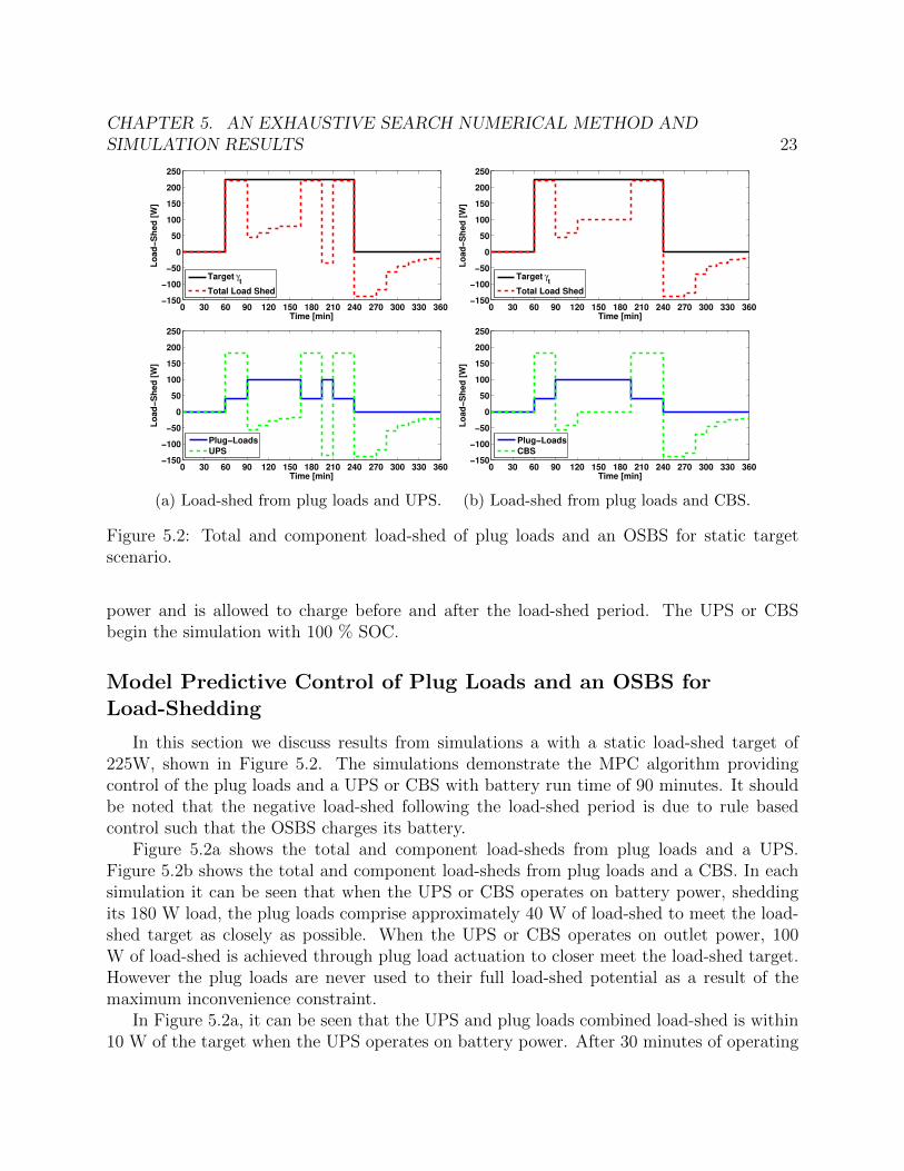
In this section we discuss results from simulations a with a static load-shed target of225W, shown in Figure 5.2. The simulations demonstrate the MPC algorithm providingcontrol of the plug loads and a UPS or CBS with battery run time of 90 minutes. It shouldbe noted that the negative load-shed following the load-shed period is due to rule basedcontrol such that the OSBS charges its battery.
Figure 5.2a shows the total and component load-sheds from plug loads and a UPS.Figure 5.2b shows the total and component load-sheds from plug loads and a CBS. In eachsimulation it can be seen that when the UPS or CBS operates on battery power, sheddingits 180 W load, the plug loads comprise approximately 40 W of load-shed to meet the load-shed target as closely as possible. When the UPS or CBS operates on outlet power, 100W of load-shed is achieved through plug load actuation to closer meet the load-shed target.However the plug loads are never used to their full load-shed potential as a result of themaximum inconvenience constraint.
In Figure 5.2a, it can be seen that the UPS and plug loads combined load-shed is within10 W of the target when the UPS operates on battery power. After 30 minutes of operating
CHAPTER 5. AN EXHAUSTIVE SEARCH NUMERICAL METHOD ANDSIMULATION RESULTS 24
on battery power, the UPS charges its battery for 75 minutes. The UPS then operates onbattery power for 30 minutes before returning to outlet power. At this point the UPS isdrawing 140 W to charge, while the plug loads contribute 100 W to the load-shed, thus thereis actually a negative load-shed of 40 W.
In Figure 5.2b, it can be seen that the CBS operates on battery power for the first30 minutes of the load-shed period. It then operates on outlet power and charges for 30minutes, before operating on outlet power without charging for 75 minutes. During thistime, the plug loads constitute the load-shed of 100 W. For the last 45 minutes of the event,the CBS operates on battery power, and the plug loads constitute 40 W of load-shed.
In Figure 5.2, it can be seen that the UPS runs on battery power for a total of 90 minutes,while the CBS does so for 75 minutes. The UPS charges its battery for more time than theCBS, during the times either OSBS draws outlet power. The time from 120 minutes to 195minutes in which the CBS operates on outlet power without charging its battery highlightsthat doing so is optimal for certain conditions.
Demand Response Scenario
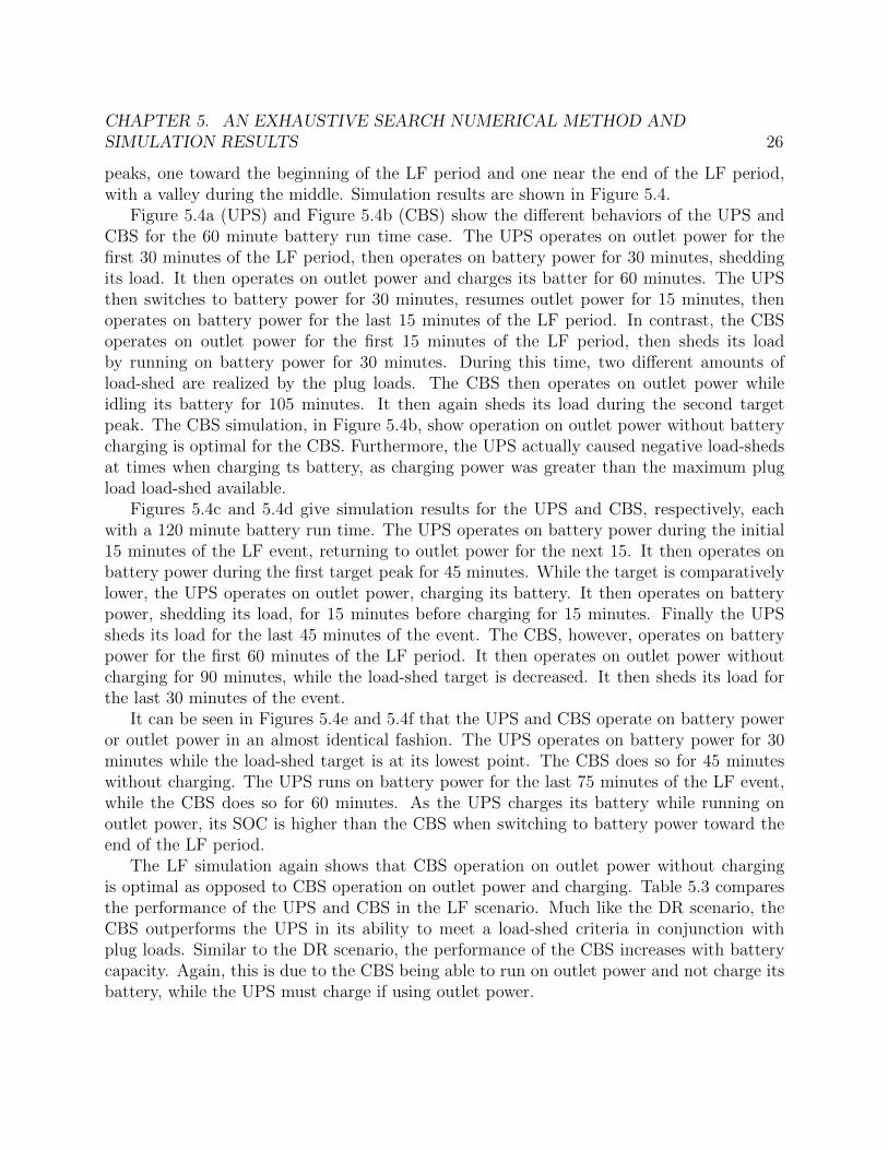
In the demand response scenario, a static load-shed target of 225W was assigned overthe 180 minute load-shed period. Simulation results for three battery capacity cases, forboth the UPS and CBS, are shown in Figure 5.3. The figures show the load-shed target andthe total load-shed achieved when using plug loads and either the UPS (red, left column) orCBS (blue, right column). It can be seen that the UPS and CBS generally exhibit similarbehavior at the end of the DR period independent of batter capacity. They both reserveand/or charge to accrue enough SOC to operate on battery power such that the battery ismaximally discharged by the end of the DR period.
Figures 5.3a and 5.3b show simulation results for a UPS and CBS with 60 minute batteryrun times, respectively. Both operate on outlet power from the beginning of the event, withplug loads constituting the load-shed of 100 W. Starting 45 minutes prior to the end ofthe event, both the UPS and CBS operate on battery power, shedding their load. Duringthis time plug loads contribute 40 W of load-shed, instead of the prior 100 W. Similar tothe results from Figure 5.2 the plug load inconvenience constrains prevents their load-shedpotential from being fully realized when the OSBS operates on outlet power.
Simulation results for the 120 minute run time case are shown in Figure 5.3c and 5.3d.It can be seen that the UPS and CBS exhibit similar behavior during the DR period. Theyboth operate on battery power for the initial 15 minutes of the DR period, then operateon outlet power. The UPS charges its battery as it must, while the CBS does not. At 75minutes from the end of the DR period, both the UPS and CBS operate on battery power,shedding their respective loads.
Figure 5.3e and Figure 5.3f show the results from the 180 minute run time case for theUPS and CBS, respectively. The UPS and CBS both shed their loads by operating on batterypower for the first 60 minutes of the DR period. They then both operate on outlet power for45 minutes. During this time the UPS charges its battery and the CBS does not. Both the
CHAPTER 5. AN EXHAUSTIVE SEARCH NUMERICAL METHOD ANDSIMULATION RESULTS 25
UPS and CBS operate on battery power for the last 75 minutes of the DR period, sheddingtheir respective loads.
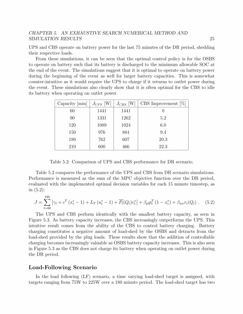
From these simulations, it can be seen that the optimal control policy is for the OSBSto operate on battery such that its battery is discharged to the minimum allowable SOC atthe end of the event. The simulations suggest that it is optimal to operate on battery powerduring the beginning of the event as well for larger battery capacities. This is somewhatcounter-intuitive as it would require the UPS to charge if it returns to outlet power duringthe event. These simulations also clearly show that it is often optimal for the CBS to idleits battery when operating on outlet power.
Capacity [min] JUPS [W] JCBS [W] CBS Improvement [%]
60 1441 1441 0
90 1331 1262 5.2
120 1089 1024 6.0
150 976 884 9.4
180 762 607 20.3
210 600 466 22.3
Table 5.2: Comparison of UPS and CBS performance for DR scenario.
Table 5.2 compares the performance of the UPS and CBS from DR scenario simulations.Performance is measured as the sum of the MPC objective function over the DR period,evaluated with the implemented optimal decision variables for each 15 minute timestep, asin (5.2):
J =240∑t=60
∣∣γt + cT (x∗t − 1) + LT (u∗t − 1) + Pt(Qt)v∗t
∣∣+ βplpTt (1− x∗t ) + βsocrt(Qt) . (5.2)
The UPS and CBS perform identically with the smallest battery capacity, as seen inFigure 5.3. As battery capacity increases, the CBS increasingly outperforms the UPS. Thisintuitive result comes from the ability of the CBS to control battery charging. Batterycharging constitutes a negative amount of load-shed by the OSBS and detracts from theload-shed provided by the plug loads. These results show that the addition of controllablecharging becomes increasingly valuable as OSBS battery capacity increases. This is also seenin Figure 5.3 as the CBS does not charge its battery when operating on outlet power duringthe DR period.
Load-Following Scenario
In the load following (LF) scenario, a time varying load-shed target is assigned, withtargets ranging from 75W to 225W over a 180 minute period. The load-shed target has two
CHAPTER 5. AN EXHAUSTIVE SEARCH NUMERICAL METHOD ANDSIMULATION RESULTS 26
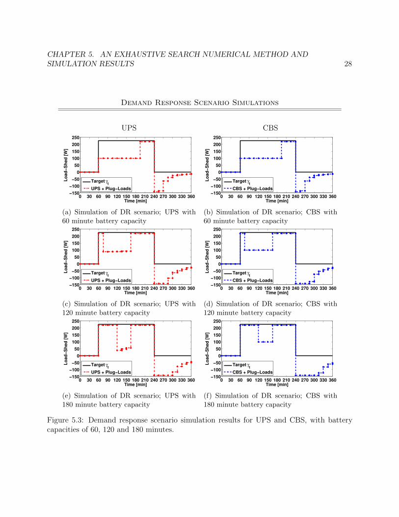
peaks, one toward the beginning of the LF period and one near the end of the LF period,with a valley during the middle. Simulation results are shown in Figure 5.4.
Figure 5.4a (UPS) and Figure 5.4b (CBS) show the different behaviors of the UPS andCBS for the 60 minute battery run time case. The UPS operates on outlet power for thefirst 30 minutes of the LF period, then operates on battery power for 30 minutes, sheddingits load. It then operates on outlet power and charges its batter for 60 minutes. The UPSthen switches to battery power for 30 minutes, resumes outlet power for 15 minutes, thenoperates on battery power for the last 15 minutes of the LF period. In contrast, the CBSoperates on outlet power for the first 15 minutes of the LF period, then sheds its loadby running on battery power for 30 minutes. During this time, two different amounts ofload-shed are realized by the plug loads. The CBS then operates on outlet power whileidling its battery for 105 minutes. It then again sheds its load during the second targetpeak. The CBS simulation, in Figure 5.4b, show operation on outlet power without batterycharging is optimal for the CBS. Furthermore, the UPS actually caused negative load-shedsat times when charging ts battery, as charging power was greater than the maximum plugload load-shed available.
Figures 5.4c and 5.4d give simulation results for the UPS and CBS, respectively, eachwith a 120 minute battery run time. The UPS operates on battery power during the initial15 minutes of the LF event, returning to outlet power for the next 15. It then operates onbattery power during the first target peak for 45 minutes. While the target is comparativelylower, the UPS operates on outlet power, charging its battery. It then operates on batterypower, shedding its load, for 15 minutes before charging for 15 minutes. Finally the UPSsheds its load for the last 45 minutes of the event. The CBS, however, operates on batterypower for the first 60 minutes of the LF period. It then operates on outlet power withoutcharging for 90 minutes, while the load-shed target is decreased. It then sheds its load forthe last 30 minutes of the event.
It can be seen in Figures 5.4e and 5.4f that the UPS and CBS operate on battery poweror outlet power in an almost identical fashion. The UPS operates on battery power for 30minutes while the load-shed target is at its lowest point. The CBS does so for 45 minuteswithout charging. The UPS runs on battery power for the last 75 minutes of the LF event,while the CBS does so for 60 minutes. As the UPS charges its battery while running onoutlet power, its SOC is higher than the CBS when switching to battery power toward theend of the LF period.
The LF simulation again shows that CBS operation on outlet power without chargingis optimal as opposed to CBS operation on outlet power and charging. Table 5.3 comparesthe performance of the UPS and CBS in the LF scenario. Much like the DR scenario, theCBS outperforms the UPS in its ability to meet a load-shed criteria in conjunction withplug loads. Similar to the DR scenario, the performance of the CBS increases with batterycapacity. Again, this is due to the CBS being able to run on outlet power and not charge itsbattery, while the UPS must charge if using outlet power.

CHAPTER 5. AN EXHAUSTIVE SEARCH NUMERICAL METHOD ANDSIMULATION RESULTS 27
Capacity [min] JUPS [W] JCBS [W] CBS Improvement [%]
60 1183 1118 5.5
90 1100 968 12
120 876 736 16
150 683 556 18.6
180 450 357 20.7
210 389 256 34.2
Table 5.3: Comparison of UPS and CBS performance for LF scenario.
Remarks on Exhaustive Search Method and Simulations
Simulation results show that the CBS offers better performance than the UPS for boththe DR and LF scenarios. The performance gap increases as battery size increases. Thisintuitive result comes as the CBS offers more flexibility as it can run on outlet power and notcharge its battery. Simulation results also highlight that it is very often optimal for the CBSto utilize this feature during a DR or LF event. This can be seen in Figure 5.4, where theCBS does not charge its battery while running on outlet power, when the load-shed targetis relatively low. Of course, with a low enough load-shed target it may be optimal to chargethe CBS battery, especially if plug loads can be actuated to account for the charging powerdrawn.
While the exhaustive search method delivers an optimal control policy at each timestep,it suffers from several drawbacks. The main drawback is the length of the prediction horizonN . The optimal control policy may not take important future events into account. As theprediction horizon N needs to be small enough for computational expediency, the lengthof the timesteps also becomes an issue. With a timestep that is too small, the temporallength of the prediction horizon may be too short to capture important future events and/orto capture different battery charging regimes. This can be remedied by increasing timesteplength. However the OSBS charging power is then averaged over a longer time. These caveatsassociated with the exhaustive search method prompt the search for a different method forsolving the optimization program, which will be discussed in the next chapter.
CHAPTER 5. AN EXHAUSTIVE SEARCH NUMERICAL METHOD ANDSIMULATION RESULTS 28
Demand Response Scenario Simulations
UPS CBS
0 30 60 90 120 150 180 210 240 270 300 330 360−150
−100
−50
0
50
100
150
200
250
Time [min]
Lo
ad
−S
hed
[W
]
Target γt
UPS + Plug−Loads
(a) Simulation of DR scenario; UPS with60 minute battery capacity
0 30 60 90 120 150 180 210 240 270 300 330 360−150
−100
−50
0
50
100
150
200
250
Time [min]
Lo
ad
−S
hed
[W
]
Target γt
CBS + Plug−Loads
(b) Simulation of DR scenario; CBS with60 minute battery capacity
0 30 60 90 120 150 180 210 240 270 300 330 360−150
−100
−50
0
50
100
150
200
250
Time [min]
Lo
ad
−S
hed
[W
]
Target γt
UPS + Plug−Loads
(c) Simulation of DR scenario; UPS with120 minute battery capacity
0 30 60 90 120 150 180 210 240 270 300 330 360−150
−100
−50
0
50
100
150
200
250
Time [min]
Lo
ad
−S
hed
[W
]
Target γt
CBS + Plug−Loads
(d) Simulation of DR scenario; CBS with120 minute battery capacity
0 30 60 90 120 150 180 210 240 270 300 330 360−150
−100
−50
0
50
100
150
200
250
Time [min]
Lo
ad
−S
hed
[W
]
Target γt
UPS + Plug−Loads
(e) Simulation of DR scenario; UPS with180 minute battery capacity
0 30 60 90 120 150 180 210 240 270 300 330 360−150
−100
−50
0
50
100
150
200
250
Time [min]
Lo
ad
−S
hed
[W
]
Target γt
CBS + Plug−Loads
(f) Simulation of DR scenario; CBS with180 minute battery capacity
Figure 5.3: Demand response scenario simulation results for UPS and CBS, with batterycapacities of 60, 120 and 180 minutes.
CHAPTER 5. AN EXHAUSTIVE SEARCH NUMERICAL METHOD ANDSIMULATION RESULTS 29
Load-Following Simulations
UPS CBS
0 30 60 90 120 150 180 210 240 270 300 330 360−150
−100
−50
0
50
100
150
200
250
Time [min]
Lo
ad
−S
hed
[W
]
Target γt
UPS + Plug−Loads
(a) Simulation of LF Scenario; UPS with 60minute battery capacity
0 30 60 90 120 150 180 210 240 270 300 330 360−150
−100
−50
0
50
100
150
200
250
Time [min]
Lo
ad
−S
hed
[W
]
Target γt
CBS + Plug−Loads
(b) Simulation of LF Scenario; CBS with60 minute battery capacity
0 30 60 90 120 150 180 210 240 270 300 330 360−150
−100
−50
0
50
100
150
200
250
Time [min]
Lo
ad
−S
hed
[W
]
Target γt
UPS + Plug−Loads
(c) Simulation of LF Scenario; UPS with120 minute battery capacity
0 30 60 90 120 150 180 210 240 270 300 330 360−150
−100
−50
0
50
100
150
200
250
Time [min]
Lo
ad
−S
hed
[W
]
Target γt
CBS + Plug−Loads
(d) Simulation of LF Scenario; CBS with120 minute battery capacity
0 30 60 90 120 150 180 210 240 270 300 330 360−150
−100
−50
0
50
100
150
200
250
Time [min]
Lo
ad
−S
hed
[W
]
Target γt
UPS + Plug−Loads
(e) Simulation of LF Scenario; UPS with180 minute battery capacity
0 30 60 90 120 150 180 210 240 270 300 330 360−150
−100
−50
0
50
100
150
200
250
Time [min]
Lo
ad
−S
hed
[W
]
Target γt
CBS + Plug−Loads
(f) Simulation of LF Scenario; CBS with180 minute battery capacity
Figure 5.4: Load-following scenario simulation results for UPS and CBS, with battery ca-pacities of 60, 120 and 180 minutes.

30
Chapter 6
A Dynamic Programming Algorithmfor the MPC Optimization Programand Simulation Results
6.1 Dynamic Programming Algorithm
Dynamic programming is a powerful optimization tool, that can be used to solve manycomplex problems not amenable to linear or quadratic programs. The basic tenet is todissolve a problem into a series of smaller problems. As in [21], [46] it is used to optimizebased on a set of predicted signals and/or events .The MPC formulation is amenable tobeing formulated as a dynamic program, addressing several of the problems associated bythe aforementioned exhaustive search method. The system state is the OSBS battery energySt, and by linear scaling the SOC Qt. The UPS effectively has one binary decision variable,and therefore has two operation states: operation on outlet battery where ut = vt = 0, andoperation on outlet power where ut = vt = 1. The CBS has two decision variables, and threeoperational states: operation on battery power where ut = vt = 0, operation on outlet powerwithout charging where ut = 1, vt = 0, and operation on outlet power with charging whereut = vt = 1.
The algorithm for solving the DP is as follows: The SOC Q is gridded as a discrete set ofpoints. At the last timestep, t = N , the boundary condition is computed for each point inthe SOC grid as rN(QN) and is stored as the terminal cost VN(QN). The algorithm proceedsto the previous timestep, t = N − 1. At each SOC grid point Qj the OSBS dynamics(4.2) and (4.4) are evolved over one timestep for the two (UPS) or three (CBS) operationstates. For Qj
t , this gives the battery energy St+1(Sjt , ut, vt), and SOC Qt+1(Q
jt , ut, vt) by
(4.1) at the next time step, and the average charging power over the timestep Pt(Qjt). The
feasibility of each OSBS operation state is checked using Qt+1(Qjt , ut, vt) in the minimum
SOC constraint (3.6d). If an operation state is feasible, a binary integer linear program (6.1)gives the optimal plug load decision variable x∗t (Q
jt , ut, vt) as a function of the OSBS SOC
CHAPTER 6. A DYNAMIC PROGRAMMING ALGORITHM FOR THE MPCOPTIMIZATION PROGRAM AND SIMULATION RESULTS 31
and operation state for the current timestep:
x∗t (Qjt , ut, vt) = argmin
xt
{∣∣γt + cT (xt − 1) + LT (ut − 1) + Pt(Qjt)vt∣∣+ βplp
Tt (1− xt)
}subject to pTt (1− xt) ≤ σt
xt ∈ χtxit ∈ {0, 1} ∀i .
(6.1)The stage cost is computed for each operation state, as in (6.2), using the average charging
power and the optimal plug load states x∗t (Qt, ut, vt) for the operation state:
gt(Qjt , ut, vt) =
∣∣γt + cT(xj∗t (Qj
t , ut, vt)− 1)
+ LT (ut − 1) + Pt(Qjt)vt∣∣ . . .
+ βplpTt
(1− xj∗t (Qj
t , ut, vt))
+ βsocrt(Qjt) .
(6.2)
The cost-to-go function (6.3) is evaluated for feasible OSBS operation states, using a lin-ear interpolation to calculate Vt+1(Qt+1(Q
jt , ut, vt)). The OSBS operation state, and therefore
decision variables, that minimizes vjt (Qjt) is chosen as the optimal:
v∗t (Qjt) = min
ut,vt
{gt(Q
jt , ut, vt) + Vt+1(Qt+1(Q
jt , ut, vt))
}. (6.3)
Evaluating (6.3) gives the optimal OSBS decision variables u∗t (Qjt) and v∗t (Q
jt) at time t
and for SOC point Qjt . This also gives the optimal plug load decision variable x∗t (Q
jt). The
optimal decision variables are saved in lookup tables indexed by time and SOC. The cost-to-go v∗t (Q
jt) is stored for the current timestep and SOC. This algorithm proceeds backwards
in time until the initial timestep, at which point it is terminated. The DP algorithm is alsooutlined below:
1. At t = N , initialize cost-to-go function VN(QN) using boundary condition of rN(QN)for all SOCs grid points.
2. Proceed backward one timestep and loop through all SOC grid points.
3. At the current SOC grid point Qjt , compute St+1(Q
jt) by (4.2), Qt+1(Q
jt) by (4.1),
Pt(Qjt) by (4.4), and rt(Q
jt) by (3.7) for each operation state.
4. Check feasibility of operation state with regard to battery SOC (3.6d).
- If operation state is infeasible and vt = 0, set cost-to-go for operation state toinfinity.
- If operation state is infeasible and vt = 1, solve BILP (6.1) and compute stagecost (6.2) for operation state.
- If operation state is feasible, solve BILP (6.1) and compute stage cost (6.2) foroperation state.

CHAPTER 6. A DYNAMIC PROGRAMMING ALGORITHM FOR THE MPCOPTIMIZATION PROGRAM AND SIMULATION RESULTS 32
5. Select optimal OSBS and plug load operation state for SOC grid point via (6.3).
6. Store optimal decision variables u∗t (Qjt), v
∗t (Q
jt), x
∗t (Q
jt), and cost-to-go v∗t (Q
jt) for
current SOC.
7. Repeat steps 3 through 6 for all SOC grid points at current time t.
8. Repeat steps 2 through 7 progressing backward in time through first timestep t = 1.Terminate after.
Casting the MPC as a dynamic program eliminates several of the problems of the exhaus-tive search method. While the DP algorithm has advantages in solving the MPC optimizationprogram, it also has drawbacks. The most recognizable is the preclusion of solving an op-timization program with multiple OSBS systems within a domain. For k OSBS systems,each with SOC grid of size n, there are nk possible SOC combinations. At each of thesecombinations every possible control state over the k OSBS systems must be compared, up tok3. It can clearly be seen that this method is not scalable in the number of OSBS systems,as computation scales exponentially.
6.2 Simulation Results using Dynamic Programming
Algorithm
In this section we present simulation results for two scenarios. The first scenario is of ademand response (DR) event in which a static load-shed target is assigned to the EIG froma higher building level authority. The second is a load-following (LF) scenario where a timevarying load-shed target is assigned. The load-shed targets for both scenarios are shown inFigure 5.1 for simulation periods (event length) of 180 minutes. The timestep length is one(1) minute.
The simulations are of an EIG coordinating the listed plug loads and either a UPS orCBS. As in the simulations for the exhaustive search method, we select a variety of plugloads representing commonly found devices in commercial offices [3, 42]. The plug loads andtheir respective power consumption and occupant assigned static inconvenience value arelisted in Table 5.1.
The UPS and CBS have identical parameters and battery models. We look at one batterycapacity for these simulations; 180 minutes. The plug load served by the OSBS is 120 W,and the OSBS operating power is 60 W. The total load on the OSBS is LT = 180 W.The minimum SOC is 25%, to simulate battery longevity considerations and to represent areserve of battery energy desired by the occupant. The plug load inconvenience weighting isβpl = 25, and SOC inconvenience weighting is βsoc = 50. The SOC inconvenience functionrt(Qt) is given by (3.7) with values of Qq = 40 and rr = 0.1, and can be seen in Figure3.2. In each scenario, we assume the OSBS operates on outlet power before and after theload-shed period, however we do not limit the initial SOC to 100 % SOC.
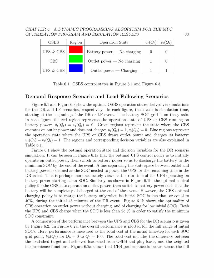
CHAPTER 6. A DYNAMIC PROGRAMMING ALGORITHM FOR THE MPCOPTIMIZATION PROGRAM AND SIMULATION RESULTS 33
OSBS Region Operation State ut(Qt) vt(Qt)
UPS & CBS Battery power — No charging 0 0
CBS Outlet power — No charging 1 0
UPS & CBS Outlet power — Charging 1 1
Table 6.1: OSBS control states in Figure 6.1 and Figure 6.3.
Demand Response Scenario and Load-Following Scenarios
Figure 6.1 and Figure 6.3 show the optimal OSBS operation states derived via simulationsfor the DR and LF scenarios, respectively. In each figure, the x axis is simulation time,starting at the beginning of the DR or LF event. The battery SOC grid is on the y axis.In each figure, the red region represents the operation state of UPS or CBS running onbattery power: ut(Qt) = vt(Qt) = 0. Green regions represent the state where the CBSoperates on outlet power and does not charge: ut(Qt) = 1, vt(Qt) = 0. Blue regions representthe operation state where the UPS or CBS draws outlet power and charges its battery:ut(Qt) = vt(Qt) = 1. The regions and corresponding decision variables are also explained inTable 6.1.
Figure 6.1 show the optimal operation state and decision variables for the DR scenariosimulation. It can be seen in Figure 6.1a that the optimal UPS control policy is to initiallyoperate on outlet power, then switch to battery power so as to discharge the battery to theminimum SOC by the end of the event. A line separating the state space between outlet andbattery power is defined as the SOC needed to power the UPS for the remaining time in theDR event. This is perhaps more accurately views as the run time of the UPS operating onbattery power starting at an SOC. Similarly, as shown in Figure 6.1b, the optimal controlpolicy for the CBS is to operate on outlet power, then switch to battery power such that thebattery will be completely discharged at the end of the event. However, the CBS optimalcharging policy is to charge the battery only when its initial SOC is less than or equal to40%, during the initial 45 minutes of the DR event. Figure 6.1b shows the optimality ofCBS operation on outlet power without charging, and of charging for low initial SOCs. Boththe UPS and CBS charge when the SOC is less than 25 % in order to satisfy the minimumSOC constraint.
A comparison of the performance between the UPS and CBS for the DR scenario is givenby Figure 6.2. In Figure 6.2a, the overall performance is plotted for the full range of initialSOCs. Here, performance is measured as the total cost at the initial timestep for each SOCgrid point, V0(Q0) for Q0 = 0 to Q0 = 100. The total cost includes the difference betweenthe load-shed target and achieved load-shed from OSBS and plug loads, and the weightedinconvenience functions. Figure 6.2a shows that CBS performance is better across the full
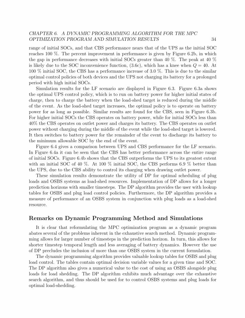
CHAPTER 6. A DYNAMIC PROGRAMMING ALGORITHM FOR THE MPCOPTIMIZATION PROGRAM AND SIMULATION RESULTS 34
range of initial SOCs, and that CBS performance nears that of the UPS as the initial SOCreaches 100 %. The percent improvement in performance is given by Figure 6.2b, in whichthe gap in performance decreases with initial SOCs greater than 40 %. The peak at 40 %is likely due to the SOC inconvenience function, (3.6c), which has a knee when Q = 40. At100 % initial SOC, the CBS has a performance increase of 3.0 %. This is due to the similaroptimal control policies of both devices and the UPS not charging its battery for a prolongedperiod with high initial SOCs.
Simulation results for the LF scenario are displayed in Figure 6.3. Figure 6.3a showsthe optimal UPS control policy, which is to run on battery power for higher initial states ofcharge, then to charge the battery when the load-shed target is reduced during the middleof the event. As the load-shed target increases, the optimal policy is to operate on batterypower for as long as possible. Similar results are found for the CBS, seen in Figure 6.3b.For higher initial SOCs the CBS operates on battery power, while for initial SOCs less than40% the CBS operates on outlet power and charges its battery. The CBS operates on outletpower without charging during the middle of the event while the load-shed target is lowered.It then switches to battery power for the remainder of the event to discharge its battery tothe minimum allowable SOC by the end of the event.
Figure 6.4 gives a comparison between UPS and CBS performance for the LF scenario.In Figure 6.4a it can be seen that the CBS has better performance across the entire rangeof initial SOCs. Figure 6.4b shows that the CBS outperforms the UPS to its greatest extentwith an initial SOC of 40 %. At 100 % initial SOC, the CBS performs 6.9 % better thanthe UPS, due to the CBS ability to control its charging when drawing outlet power.
These simulation results demonstrate the utility of DP for optimal scheduling of plugloads and OSBS systems as load-shed resources. Implementation of DP allows for a longerprediction horizons with smaller timesteps. The DP algorithm provides the user with lookuptables for OSBS and plug load control policies. Furthermore, the DP algorithm provides ameasure of performance of an OSBS system in conjunction with plug loads as a load-shedresource.
Remarks on Dynamic Programming Method and Simulations
It is clear that reformulating the MPC optimization program as a dynamic programabates several of the problems inherent in the exhaustive search method. Dynamic program-ming allows for larger number of timesteps in the prediction horizon. In turn, this allows forshorter timestep temporal length and less averaging of battery dynamics. However the useof DP precludes the inclusion of more than one OSBS system in the current formulation.
The dynamic programming algorithm provides valuable lookup tables for OSBS and plugload control. The tables contain optimal decision variable values for a given time and SOC.The DP algorithm also gives a numerical value to the cost of using an OSBS alongside plugloads for load shedding. The DP algorithm exhibits much advantage over the exhaustivesearch algorithm, and thus should be used for to control OSBS systems and plug loads foroptimal load-shedding.
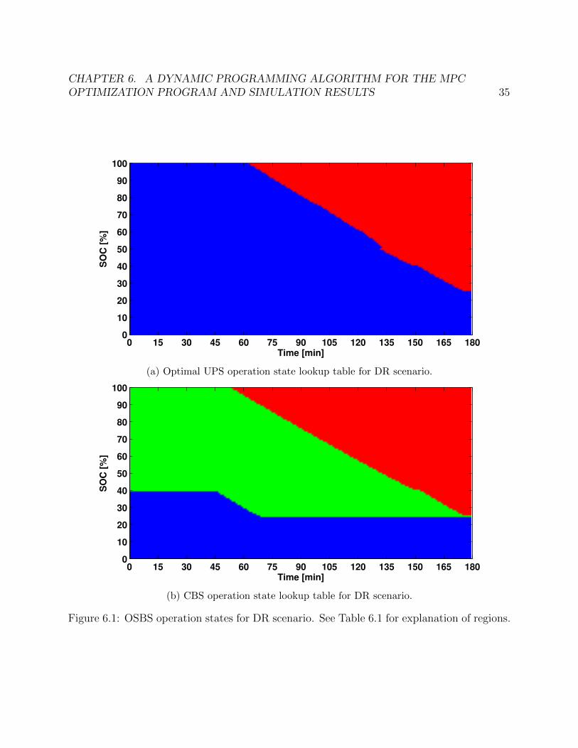
CHAPTER 6. A DYNAMIC PROGRAMMING ALGORITHM FOR THE MPCOPTIMIZATION PROGRAM AND SIMULATION RESULTS 35
Time [min]
SO
C [
%]
0 15 30 45 60 75 90 105 120 135 150 165 1800
10
20
30
40
50
60
70
80
90
100
(a) Optimal UPS operation state lookup table for DR scenario.
Time [min]
SO
C [
%]
0 15 30 45 60 75 90 105 120 135 150 165 1800
10
20
30
40
50
60
70
80
90
100
(b) CBS operation state lookup table for DR scenario.
Figure 6.1: OSBS operation states for DR scenario. See Table 6.1 for explanation of regions.
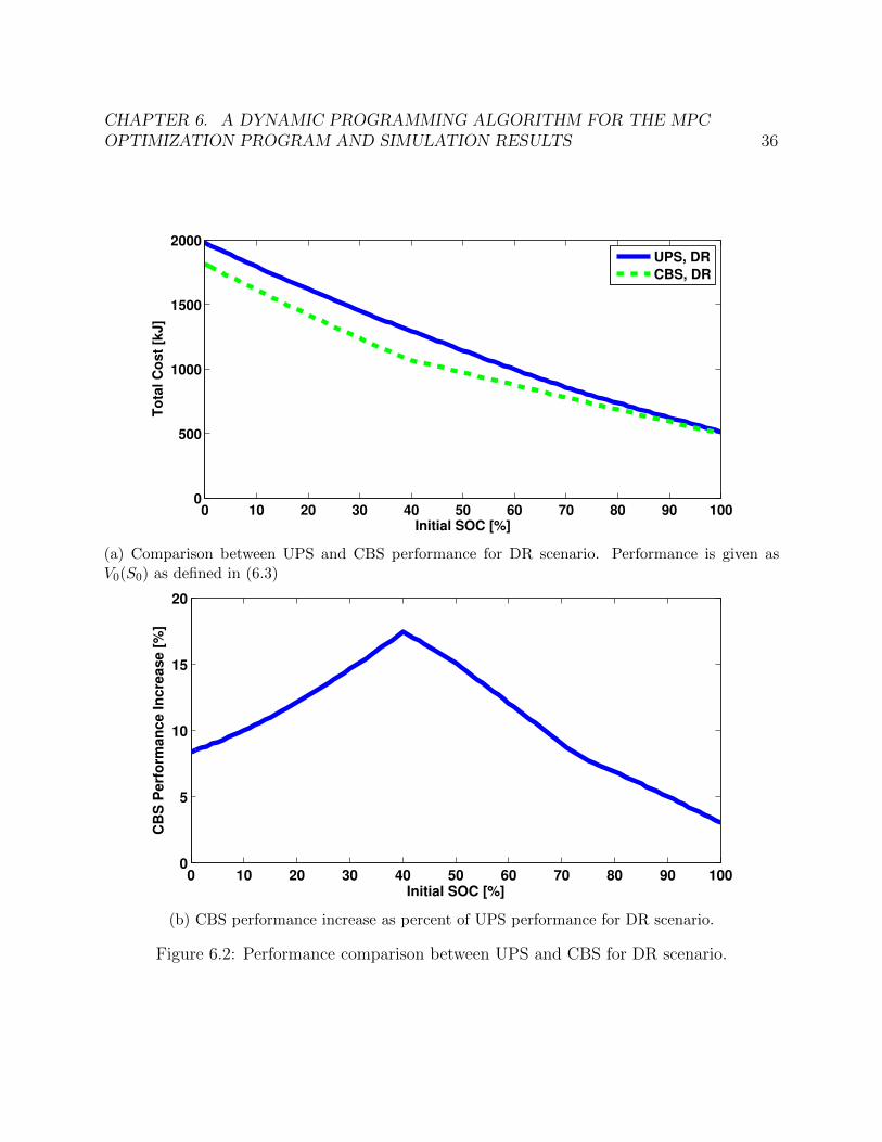
CHAPTER 6. A DYNAMIC PROGRAMMING ALGORITHM FOR THE MPCOPTIMIZATION PROGRAM AND SIMULATION RESULTS 36
0 10 20 30 40 50 60 70 80 90 1000
500
1000
1500
2000
Initial SOC [%]
To
tal C
ost
[kJ]
UPS, DR
CBS, DR
(a) Comparison between UPS and CBS performance for DR scenario. Performance is given asV0(S0) as defined in (6.3)
0 10 20 30 40 50 60 70 80 90 1000
5
10
15
20
Initial SOC [%]
CB
S P
erf
orm
an
ce In
cre
ase [
%]
(b) CBS performance increase as percent of UPS performance for DR scenario.
Figure 6.2: Performance comparison between UPS and CBS for DR scenario.
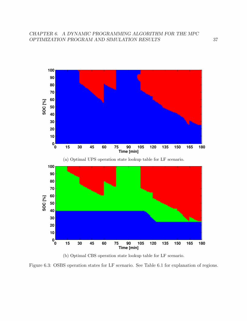
CHAPTER 6. A DYNAMIC PROGRAMMING ALGORITHM FOR THE MPCOPTIMIZATION PROGRAM AND SIMULATION RESULTS 37
Time [min]
SO
C [
%]
0 15 30 45 60 75 90 105 120 135 150 165 1800
10
20
30
40
50
60
70
80
90
100
(a) Optimal UPS operation state lookup table for LF scenario.
Time [min]
SO
C [
%]
0 15 30 45 60 75 90 105 120 135 150 165 1800
10
20
30
40
50
60
70
80
90
100
(b) Optimal CBS operation state lookup table for LF scenario.
Figure 6.3: OSBS operation states for LF scenario. See Table 6.1 for explanation of regions.
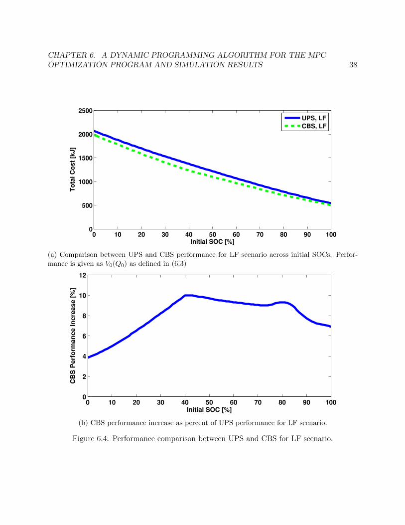
CHAPTER 6. A DYNAMIC PROGRAMMING ALGORITHM FOR THE MPCOPTIMIZATION PROGRAM AND SIMULATION RESULTS 38
0 10 20 30 40 50 60 70 80 90 1000
500
1000
1500
2000
2500
Initial SOC [%]
To
tal C
ost
[kJ]
UPS, LF
CBS, LF
(a) Comparison between UPS and CBS performance for LF scenario across initial SOCs. Perfor-mance is given as V0(Q0) as defined in (6.3)
0 10 20 30 40 50 60 70 80 90 1000
2
4
6
8
10
12
Initial SOC [%]
CB
S P
erf
orm
an
ce In
cre
ase [
%]
(b) CBS performance increase as percent of UPS performance for LF scenario.
Figure 6.4: Performance comparison between UPS and CBS for LF scenario.
39
Chapter 7
Concluding Remarks and FutureWork
In this work we present a framework for optimal control of plug loads and battery storagein the context of load-shedding. We discuss the impetus for this work, enabling technologiesand previous research efforts in the field. The use of EIG and SPS systems in a commercialoffice is discussed and a model predictive controller is formulated. This MPC balancesmeeting a load-shedding objective with the inconvenience and discomfort associated withdoing so. An OSBS battery model derived from experimental observation is discussed. TwoOSBS systems are presented, with their differences in physical key physical and mathematicalmodel difference highlighted.
The complexity of the MPC optimization program is discussed. A simplification enablesthe use of an exhaustive search method which is outlined. Simulation results for a demandresponse and a load-following scenarios are presented. Simulations show the value of batterystorage to complement plug loads as a load-shed resource. Simulations show that it is optimalto run on battery power so as to discharge it at the end of a DR or LF event. The resultsquantify the increasing value of controllable charging with battery capacity. We found thatfor the smallest battery capacities, the UPS and CBS offer identical performance. The CBSoutperforms the UPS 22.3 % in the DR scenario, and 34.2 % in the LF scenario. Thedrawbacks of this numerical method, which may preclude its practical implementation, arealso discussed.
A second numerical method for the optimization program is presented. This dynamicprogramming algorithm eliminates several of the drawbacks of the exhaustive search method,but not without its own. The DP algorithm is discussed, as are simulations performedusing it. The simulation results demonstrate that it is optimal for both the UPS and CBSto discharge their batteries to the minimum SOC by end of the event. The UPS shouldcharge/maintain its battery to/at 100 % SOC during the beginning of the event. The CBSshould only charge its battery if it has a low SOC during the beginning of the event. TheCBS very often operates on outlet power without charging. These results prove the needfor controllable charging. We found that for 100 % initial SOC, CBS performance is 3.0 %

CHAPTER 7. CONCLUDING REMARKS AND FUTURE WORK 40
better than the UPS in the DR scenario, and 6.9 % better in the LF scenario.We plan to continue this work in two key areas. The first is to investigate other methods
for solving the MPC optimization program, including binary relaxations. A second method isthe reformulation of the battery model with special ordered sets to allow for casting the MPCas a linear program. The second area in which this work will be continued is experimentationwith available hardware to verify simulation results.
41
Part II
Modeling of Unbalanced Power Flowand Optimal Control of Distributed
Energy Resources for GridReconfiguration
42
Chapter 8
Introduction
The proliferation of new types of sensors into the electric power distribution system isproviding deeper insights into the operation of the grid and is driving innovation around newparadigms for system management. Among the many new sensing devices being deployed inthe distribution grid, distribution synchrophasors provide a suite of new functionality thatcould serve to better inform the process of managing Distributed Energy Resources (DER).Distribution PMUs not only collect “traditional” system telemetry (such as voltage andcurrent magnitudes) on sub-second time intervals, but provide access to voltage and currentphase angles as well. These devices are now becoming more commonplace and are eithermanifesting as standalone units [30] or are being incorporated into other system components[44].
The growing presence of distribution PMUs indicates that sufficient infrastructure maybe in place in future grids to support control activities that make decisions based on feedervoltage measurements. In fact, a small, but growing, number of control applications thatutilize phase angle measurements have started to appear in literature. The work of [35]proposed the use of voltage angle measurements to curtail over-generation of renewables.Additionally, the authors of [47] considered voltage angle thresholds as criteria to connectrenewable generation. Both works refer to this control activity as “Angle Constrained ActiveManagement”, or ACAM.
An application for distribution PMU data may be useful is enabling fast and safe switch-ing of network elements. The ability to disconnect and reconnect microgrids and quicklyreconfigure distribution networks are two important abilities of future distribution networks[15, 16, 37]. Network Reconfiguration and microgrid islanding/reconnection may requireswitching actions.
Preventing arcing and or large transient currents when opening or closing a switch isimportant for safe and reliable grid operation, and to prolong the life of existing protectionequipment. To open a switch, the magnitude of the current, and therefore power, flowingthrough the line must not be over safe limits, as well as the switch action to occur at a currentzero-crossing. To close a switch, the voltage difference across it end must be sufficiently smallto prevent arcing and large current surges.

CHAPTER 8. INTRODUCTION 43
As such, distribution system operators (DSOs) require power injection at reconfigura-tion locations to close switches and minimize impact on grid components and power quality.Switching actions may be scheduled beforehand, but for a contingency case a mobile gener-ation that provides power to the correct location may be dispatched.
The advent and proliferation of distributed energy resources present an opportunity topower sections of a network and facilitate network reconfiguration at a potentially fastertimescale than current practices. With proper location of DER and sufficient power/energyresource it may be possible to control voltage and current phasors at critical points in thenetwork from the DSO, without needing to dispatch a mobile generation unit or engineeringteam.
The literature on control and optimization of DER to for more sophisticated operationdistribution networks is quite vast. Many of the works in this field seek are motivated froman economic standpoint, and works in which the aim is to directly control voltage phasors issparse.
Many works in the field study the use of semidefinite programming (SDP), semidefiniterelaxations (SDR), and convex relaxations in optimal power flow (OPF) problems. Workson this topic range from studying the geometry of the problem [23], to conditions underwhich a convex relaxation in likely to be tight [22], to limitations on the application of SDPs[24], to solving distributed SDP OPFs for unbalanced networks [11]. It should be noted thatmuch of the earlier literature considers balanced networks, and only recently have unbalancednetworks been studied [11, 50].
Recently, other works in the field have studied using approximate power models, includinglinearized models [6, 14, 39], and quadratic models [13]. Other works have considered optimalDER dispatch in a model-free framework [1, 5].
To enabled control strategies for regulation of voltage phasors, we build upon a linearmodel of unbalanced power flow by adding a relation between voltage angle differences andline real and reactive power. Previous works have considered linear models of unbalancedpower flow [14, 39], but have only provided considered voltage magnitude. To our knowledge,this work is the first to include voltage angle on an unbalanced network, and in which anOPF is capable of regulating the entire voltage phasor (magnitude and angle).
In this work, we investigate OPF formulations for control of voltage magnitude andphase angle through DER dispatch, for the purposes of opening or closing a switch ona distribution network. First in Section 8.1, pertinent nomenclature and equations arepresented and explained. In Chapter 9, semidefinite programming for OPF formulationsis discussed. Section 9.2 provides an overview of the state of research on SDP OPFs andpresents an argument for the need of other OPF formulations. In Section 9.3, we deriveSDP OPFs for the control of voltage magnitude and phase angle, and discuss preliminarysimulations on simple networks.
In Chapter 10, a linearized unbalanced power flow model (LUPFM) that incorporatesvoltage angle is derived. The accuracy of the LUPFM is investigated in Chapter 11 forbenchmark IEEE test feeders. Two applications of the LUPFM are discussed in Chapter12, with Section 12.1 presenting an OPF for balancing voltage magnitude across multiple

CHAPTER 8. INTRODUCTION 44
phases at networks nodes, and Section 12.2 presenting an OPF for minimizing voltage phasordifference across the ends of an open switch.
8.1 Nomenclature, Definitions, and Preliminaries
Symbol Description Unit
N Set of network nodes in network
Pn Set of phases that exist at node n
E Set of lines (edges) in network
Pmn Set of phases that exist on line (m,n)
G Set of nodes with energy resources
V φn Voltage phasor at node n on phase φ [p.u.]
Vn Vector of voltage phasors at node n [p.u.]
Eφn Square magnitude of voltage at node n on phase φ [(p.u.)2]
En Vector of square magnitudes of voltage at node n [(p.u.)2]
θφn Phase angle of voltage phasor at node n on phase φ [-]
Θn Vector of phase angles of voltage phasors at node n [-]
iφn Load current of phase φ at node n [p.u.]
in Vector of load currents at node n [p.u.]
Zφφmn Impedance of line (m,n) on phase φ [p.u.]
Zφψmn Impedance of line (m,n) between phases φ and ψ [p.u.]
Zmn Impedance matrix of line (m,n) [p.u.]
Y φφmn Admittance of line (m,n) on phase φ [p.u.]
Y φψmn Admittance of line (m,n) between phases φ and ψ [p.u.]
Ymn Admittance matrix of line (m,n) [p.u.]
Iφmn Current phasor on phase φ on line (m,n) [p.u.]
Imn Vector of current phasors on line (m,n) [p.u.]
P φmn,m Real power on line (m,n) on phase φ at node m [p.u.]
Pmn,m Vector of real power on line (m,n) at node m [p.u.]
P φmn,n Real power on line (m,n) on phase φ at node n [p.u.]
Pmn,n Vector of real power on line (m,n) at node n [p.u.]
Qφmn,m Reactive power on line (m,n) on phase φ at node m [p.u.]
Qmn,m Vector of reactive power at node m [p.u.]
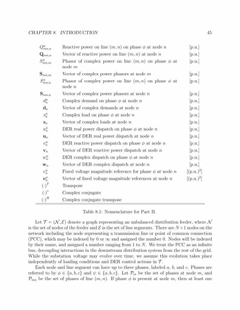
CHAPTER 8. INTRODUCTION 45
Qφmn,n Reactive power on line (m,n) on phase φ at node n [p.u.]
Qmn,n Vector of reactive power on line (m,n) at node n [p.u.]
Sφmn,m Phasor of complex power on line (m,n) on phase φ atnode m
[p.u.]
Smn,m Vector of complex power phasors at node m [p.u.]
Sφmn,n Phasor of complex power on line (m,n) on phase φ atnode n
[p.u.]
Smn,n Vector of complex power phasors at node n [p.u.]
dφn Complex demand on phase φ at node n [p.u.]
dn Vector of complex demands at node n [p.u.]
sφn Complex load on phase φ at node n [p.u.]
sn Vector of complex loads at node n [p.u.]
uφn DER real power dispatch on phase φ at node n [p.u.]
un Vector of DER real power dispatch at node n [p.u.]
vφn DER reactive power dispatch on phase φ at node n [p.u.]
vn Vector of DER reactive power dispatch at node n [p.u.]
wφn DER complex dispatch on phase φ at node n [p.u.]
wn Vector of DER complex dispatch at node n [p.u.]
eφn Fixed voltage magnitude reference for phase φ at node n [(p.u.)2]
eφn Vector of fixed voltage magnitude references at node n [(p.u.)2]
(·)T Transpose
(·)∗ Complex conjugate
(·)H Complex conjugate transpose
Table 8.1: Nomenclature for Part II.
Let T = (N , E) denote a graph representing an unbalanced distribution feeder, where Nis the set of nodes of the feeder and E is the set of line segments. There are N+1 nodes on thenetwork including the node representing a transmission line or point of common connection(PCC), which may be indexed by 0 or∞ and assigned the number 0. Nodes will be indexedby their name, and assigned a number ranging from 1 to N . We treat the PCC as an infinitebus, decoupling interactions in the downstream distribution system from the rest of the grid.While the substation voltage may evolve over time, we assume this evolution takes placeindependently of loading conditions and DER control actions in T .
Each node and line segment can have up to three phases, labeled a, b, and c. Phases arereferred to by φ ∈ {a, b, c} and ψ ∈ {a, b, c}. Let Pm be the set of phases at node m, andPmn be the set of phases of line (m,n). If phase φ is present at node m, then at least one
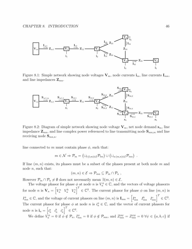
CHAPTER 8. INTRODUCTION 46
V∞ V1Z∞1
I∞1
i1
V2Z12
I12
i2
V3
Z23I23
i3
V4
Z24I24
i4
Z34
I34
V5Z45
I45i5
Figure 8.1: Simple network showing node voltages Vm, node currents im, line currents Imn,and line impedances Zmn.
V∞ V1Z∞1
S∞1,∞ S∞1,1
s1
V2Z12
S12,1 S12,2
s2
V3
Z23S23,2
S23,3
s3
V4
Z13S24,2
S24,4
s4
Z34
S34,3
S34,4
V5Z45
S45,4 S45,5
s5
Figure 8.2: Diagram of simple network showing node voltage Vm, net node demand sm, lineimpedance Zmn, and line complex power referenced to line transmitting node Smn,m and linereceiving node Smn,n.
line connected to m must contain phase φ, such that:
m ∈ N ⇒ Pm =(∪l:(l,m)∈EPlm
)∪(∪n:(m,n)∈EPmn
).
If line (m,n) exists, its phases must be a subset of the phases present at both node m andnode n, such that:
(m,n) ∈ E ⇒ Pmn ⊆ Pm ∩ Pn ,
However Pm ∩ Pn 6= ∅ does not necessarily mean ∃(m,n) ∈ E .The voltage phasor for phase φ at node n is V φ
n ∈ C, and the vectors of voltage phasorrs
for node n is Vn =[V an V b
n V cn
]T∈ C3. The current phasor for phase φ on line (m,n) is
Iφmn ∈ C, and the voltage of current phasors on line (m,n) is Imn =[Iamn Ibmn Icmn
]T∈ C3.
The current phasor for phase φ at node n is iφn ∈ C, and the vector of current phasors for
node n is in =[ian ibn icn
]T∈ C3.
We define V φn = 0 if φ /∈ Pn, Iφmn = 0 if φ /∈ Pmn, and Zφψ
mn = Zψφmn = 0 ∀ψ ∈ {a, b, c} if

CHAPTER 8. INTRODUCTION 47
φ /∈ Pmn, such that:
φ /∈ Pn ⇒ V φn = 0
φ /∈ Pmn ⇒ Iφmn = 0
φ /∈ Pmn ⇒ Zφψmn = Zψφ
mn = 0 ∀ψ ∈ {a, b, c}φ /∈ Pmn ⇒ Y φψ
mn = Y ψφmn = 0 ∀ψ ∈ {a, b, c} .
(8.1)
The current/voltage relationship for a three phase line (m,n) between adjacent nodes mand n is captured by Kirchhoff’s Voltage Laws (KVL) in its full (8.2), and compact form(8.3): V
am
V bm
V cm
=
Van
V bn
V cn
+
Zaamn Zab
mn Zacmn
Zbamn Zbb
mn Zbcmn
Zcamn Zcb
mn Zccmn
I
amn
Ibmn
Icmn
(8.2)
Vm = Vn + ZmnImn , (8.3)
where, Zφψmn = rφψmn + jxφψmn denotes the complex impedance of line (m,n) across phases φ and
ψ. Here, (8.2) and (8.3) are presented where Pmn = {a, b, c}. For lines with less than threephases (|Pmn| = 1, or |Pmn| = 2) (8.3) becomes:
[Vm]Pmn = [Vn]Pmn + [Zmn]Pmn,Pmn [Imn]Pmn , (8.4)
by employing the same indexing notation as in [11]. In this notation, rows of all terms in(8.4), and columns of Zmn, corresponding to φ /∈ Pmn are removed. For example, for a singlephase line (m,n) where Pmn = {φ}, (8.4) is stated as:
V φm = V φ
n + ZφφmnI
φmn .
For a two phase line (m,n) where Pmn = {a, b}, (8.4) is stated as:[V am
V bm
]=
[V an
V bn
]+
[Zaamn Zab
mn
Zbamn Zbb
mn
][Iamn
Ibmn
].
For a two phase line (m,n) where Pmn = {a, c}, (8.4) is stated as:[V am
V cm
]=
[V an
V cn
]+
[Zaamn Zac
mn
Zcamn Zcc
mn
][Iamn
Icmn
].
Kirchoff’s Current law at node m is given in its full (8.5) and compact (8.6) forms:
∑l:(l,m)∈E
Ialm
Iblm
Iclm
=
iam
ibm
icm
+∑
n:(m,n)∈E
Iamn
Ibmn
Icmn
(8.5)
∑l:(l,m)∈E
Ilm = im +∑
n:(m,n)∈E
Imn . (8.6)
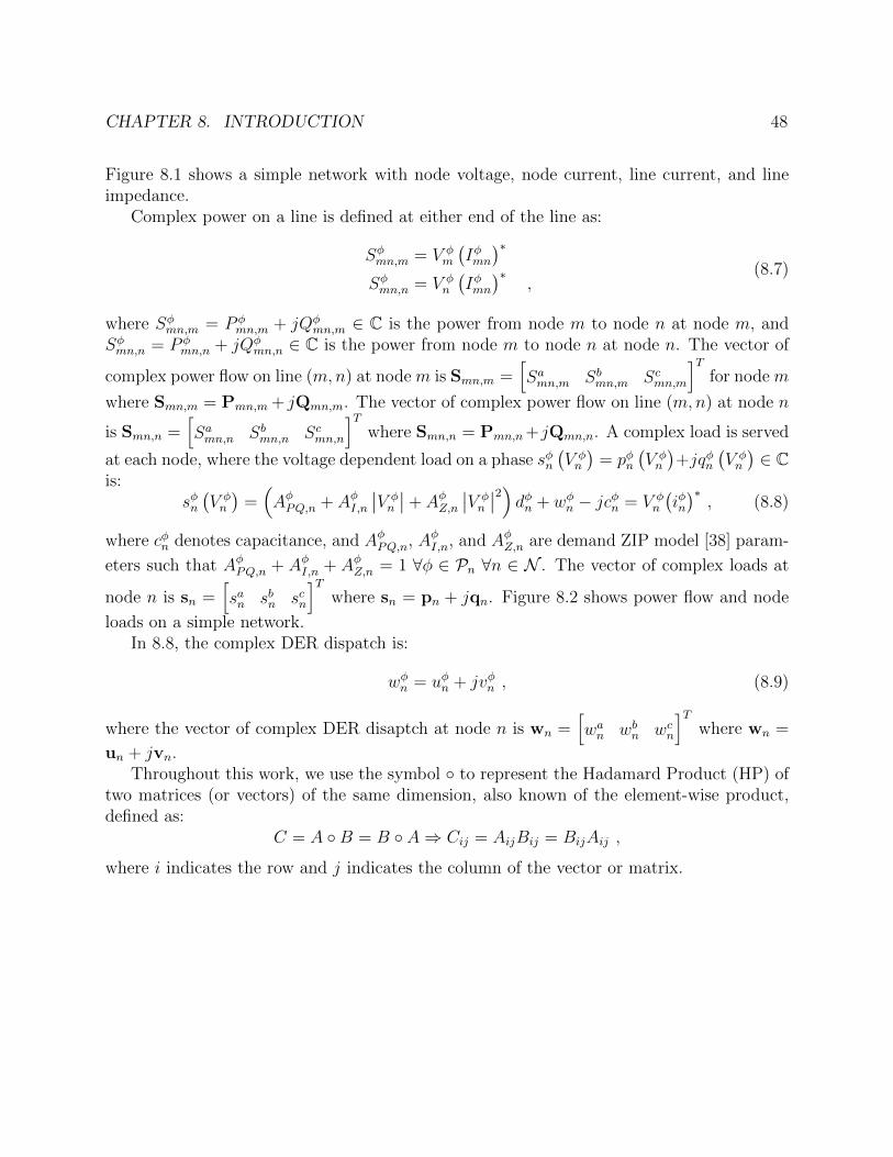
CHAPTER 8. INTRODUCTION 48
Figure 8.1 shows a simple network with node voltage, node current, line current, and lineimpedance.
Complex power on a line is defined at either end of the line as:
Sφmn,m = V φm
(Iφmn)∗
Sφmn,n = V φn
(Iφmn)∗
,(8.7)
where Sφmn,m = P φmn,m + jQφ
mn,m ∈ C is the power from node m to node n at node m, andSφmn,n = P φ
mn,n + jQφmn,n ∈ C is the power from node m to node n at node n. The vector of
complex power flow on line (m,n) at node m is Smn,m =[Samn,m Sbmn,m Scmn,m
]Tfor node m
where Smn,m = Pmn,m + jQmn,m. The vector of complex power flow on line (m,n) at node n
is Smn,n =[Samn,n Sbmn,n Scmn,n
]Twhere Smn,n = Pmn,n+jQmn,n. A complex load is served
at each node, where the voltage dependent load on a phase sφn(V φn
)= pφn
(V φn
)+jqφn
(V φn
)∈ C
is:sφn(V φn
)=(AφPQ,n + AφI,n
∣∣V φn
∣∣+ AφZ,n∣∣V φn
∣∣2) dφn + wφn − jcφn = V φn
(iφn)∗, (8.8)
where cφn denotes capacitance, and AφPQ,n, AφI,n, and AφZ,n are demand ZIP model [38] param-
eters such that AφPQ,n + AφI,n + AφZ,n = 1 ∀φ ∈ Pn ∀n ∈ N . The vector of complex loads at
node n is sn =[san sbn scn
]Twhere sn = pn + jqn. Figure 8.2 shows power flow and node
loads on a simple network.In 8.8, the complex DER dispatch is:
wφn = uφn + jvφn , (8.9)
where the vector of complex DER disaptch at node n is wn =[wan wbn wcn
]Twhere wn =
un + jvn.Throughout this work, we use the symbol ◦ to represent the Hadamard Product (HP) of
two matrices (or vectors) of the same dimension, also known of the element-wise product,defined as:
C = A ◦B = B ◦ A⇒ Cij = AijBij = BijAij ,
where i indicates the row and j indicates the column of the vector or matrix.

49
Chapter 9
A Discussion of SemidefiniteProgramming for Optimal PowerFlow Problems
9.1 Introduction
Power flow models are often nonlinear (very often quadratic) and nonconvex, due to thenonlinear relations between voltage, current, and complex power. To give an example of thenonlinear nature of power flow models, consider line (m,n) ∈ E , where the complex powerat node m is Smn,m = VmI
∗mn. A model incorporating line power flows, node voltage and line
current would therefore have quadratic equality constraints. Substituting the variable forcurrent, by using the line voltage difference divided by line admittance, Imn = Ymn (Vm − Vn),the power flow on the line at node m is Smn,m = VmY
∗mn (V ∗m − V ∗n ) = Y ∗mn (VmV
∗m − VmV ∗n ).
However, this model is now quadratic in voltage, and contains quadratic inequality con-straints. While this nonlinear equation can be linearized by variable substitution, it maybe difficult to regain the original variables. Furthermore, nonlinear constraints, especiallynonlinear equality constrains, often cause problems numerical solver convergence.
Semidefinite programming (SDP) is a useful method for transforming and approximatingoptimization programs with nonlinear or nonconvex objectives or constraints [28]. Thisis especially true for quadratic constraint quadratic programs (QCQP), which many OPFproblems are (as seen in the above example). SDP for OPF applications has been studiedextensively in recent history, with much literature addressing single phase networks, someearlier works include [7, 22]. More recent literature addresses multiphase networks [11,50]. In this work, we will use SDP as a shorthand for both semidefinite programming andsemidefinite program.
An SDP is an optimization program with a positive semidefinite matrix variable, whichwill be denoted as X. Linear operators, such as the trace, Tr(·), are often used to incorporateinequality or equality constraints and craft objective functions [28]. Constraints that are

CHAPTER 9. A DISCUSSION OF SEMIDEFINITE PROGRAMMING FOR OPTIMALPOWER FLOW PROBLEMS 50
quadratic in X can be incorporated with linear matrix inequalities. The matrix variable X,is often formed from a vector x right multiplied by its complex conjugate transpose, suchthat X = xxH . To recover the vector x from the matrix X, the solution to the SDP, X, musthave a rank of one. However, the condition that X is rank-one is not convex [28]. Thereforethis constraint is often removed from the SDP to obtain a semidefinite relaxation (SDR), aconvex relaxation of the original SDP. The SDR is better suited for solver utilizing interiorpoint methods. While a solver may not return a matrix that is strictly rank-one, if the ratioof the largest nonzero eigenvalue to the second largest nonzero eigenvalue is large enough,the matrix may be considered to be rank-one.
We now provide a summary of select literature on OPF SDPs for single and multiphasenetworks. We will discuss the successes of SDPs, and also drawbacks that may precludethem from being practically applicable.
9.2 Previous Research in SDP for OPFs
Literature on semidefinite programming has mainly focused on single phase networks,and the results show the potential of SDP and SDR as a viable method for solving nonlinearand nonconvex OPF problems. One of the earliest works utilizing SDP for OPF applicationsis [7], in which the authors derive an OPF SDP, and solve the SDP using interior pointmethods. In [22], the authors investigate conditions under which the SDP and SDR primaland dual problems will converge to the same solution, and under which a rank-one solutionis obtainable. The authors of [23] discuss geometric interpretations of power flow physics,and show that the optimal Pareto-optimal points do not change under convex relaxations.The authors also discuss line power bounds and angle constraints.
The authors of [24] investigate limitations of semidefinite programming in solving OPFproblems. They propose modifications to the SDP to replicate OPF solutions for five nodeand seven node networks. They authors found that their approach in modifying constraintswas unsuccessful, and found varying levels of success modifying the SDP objective.
The authors present simulations on simple networks that show convergence to rank-onesolutions with both binding non binding line flow constraints, with results verified by aseparate solver. However, when line flow the constraint bounds are tightened, a rank-onesolution is unobtainable, though the new problem is feasible.
The authors of [27] study sufficiency conditions for the exactness of SDP convex relax-ations; the conditions under which a rank-one solution is obtainable. The authors propose alemma (Lemma 1 in [27]) that states that a nondegenrate feasible solution to a SDP will haverank greater than 1 if the number of equality constraints plus binding inequality constraintsto the SDP is greater than or equal to twice problem dimension.
The authors propose a theorem (Theorem 2 in [27]) stating that if a primal nondegeneratesolution in the optimal solution set of the primal SDP problem has equality constraints andbinding inequality constraints in number greater than twice the problem dimensionality,then there are no rank-one solutions in the optimal solution set. This theorem places strict

CHAPTER 9. A DISCUSSION OF SEMIDEFINITE PROGRAMMING FOR OPTIMALPOWER FLOW PROBLEMS 51
bounds on the number of equality constraints that a SDP can have in order to possibly yield arank-one optimal solution, which is less than twice the problem dimensionality. The authorsprovide remarks on SDP formulation and common constraints on voltage and generation(DER dispatch).
The authors perform numerical studies on several test cases. Using test cases from liter-ature, the authors show that while all the test cases follow the sufficient condition outlinedin [27], a unique rank-one solution could not be found.
The authors then empirically investigate the effect on a network’s load profile has onobtaining an exact relaxation. They found that in gridding several loads on a network,roughly 93.7% of cases had a unique optimal solution, however only 6.3% of all cases yieldeda unique rank-one solution, so that for a vast majority of cases the relaxation is inexact.
In [29], the authors investigate implementation of an SDP OPF formulation for bothradial (acyclic) and mesh (cyclic) networks. The authors explore different formulations andline capacity constraints and their relation to obtaining an exact SDP relaxation.
The authors discuss four types of common line capacity constraints and equivalent formsfor an SDP, showing that the four line constraints have similar nonconvex feasible regions.Simulations on a simple three bus mesh network show that only one of the constraints yielda rank-1 solution for all values of maximum line voltage angle difference, while the otherthree only do so for certain values. The authors conclude from this example that problemformulation and constraint type are important to factors in successfully obtaining an exactrelaxation. The authors prove that for a mesh (cyclic) network of size 3, an exact relaxationcan be obtained if the minimum reactive DER dispatch is unbounded for a lossless case, andif the real and reactive DER dispatch is unbounded for a lossy case.
The authors then propose adding a penalty function to the OPF objective, penalizingDER reactive power dispatch, in order to obtain a low-rank or rank-1 solution. The authorsdefine a degree of sub-optimality for this modified OPF, and discuss how the modified OPFSDP solution can be used to find the global optimal solution to the original OPF.
Simulation results on mesh (cylic) test networks show that the original OPF is unable toobtain rank-1 solutions, however the modified OPF yields rank-1 solutions with appropriateweighting on the additional reactive power dispatch penalty. Simulations results also showthat the weight on the additional penalty does not significantly impact DER real powerdispatch compared to the original OPF, but does significantly alter the DER reactive powerdispatch.
In [31] and [32], the authors investigate physical network conditions that will lead to anSDP producing a globally optimal solution. The authors investigate two networks which canbe equivalently modeled, showing that the SDR converges for one and not the other.
From these examples, it can be surmised that SDP has drawbacks that may preclude itfrom being widely applicable to many different networks,
Recently, the literature on SDP OPF formulations has expanded to study multiphasenetworks. In [11], the authors derive an unblanaced multi-phase power flow model for ra-dial networks, and transform the problem into an equivalent semi-definite program (SDP)formulation. The authors discuss a convex relaxation to the equivalent SDP that such that
CHAPTER 9. A DISCUSSION OF SEMIDEFINITE PROGRAMMING FOR OPTIMALPOWER FLOW PROBLEMS 52
the relaxed equivalent SDP is convex. The authors derive a distributed solution such thatthe SDP can be implemented within subnetworks on a radial network. They leverage analgorithm using alternating direction method of multiplies (ADMM) to solve several localSDP problems accounting for a global objective and constraints.
The authors successfully transform a nonlinear optimization problem into an equivalentSDP. They furthermore apply a rank relaxation to the equivalent SDP such that the relaxedproblem is convex. The authors show that if the relaxed SDP has a solution with rank 1,then the solution is optimal for both the relaxed problem and the equivalent SDP.
The authors provide an intuitive argument that builds upon that of [23, 51], as to whythe multiphase SDP should converge to a rank-one solution for a radial (acyclic) network.While the authors present simulations that show the success of their method, for certaincases a rank-one solution was not obtainable unless the substation voltage was changed from1 to 1.02 p.u.
The authors of [50] build upon the work in [11] by developing an algorithm to solve anOPF should the convex relaxation of the SDP fail.
Literature on SDP OPFs has shown great success in utilizing SDP to solve nonlinearOPFs. However the literature also outlines several properties of SDP that may preclude itfrom being practically implementable.
9.3 Extensions of the SDP OPF for Control of
Voltage Phasors
Many of the OPFs discussed in recent literature papers are economic dispatch problems.In this section, we will derive objective functions and constraints and objective functions forcontrol of voltage phasors for the purposes of grid reconfiguration. The work in this sectionis not intended as a definitive study on SDP OPFs for controlling voltage magnitude andphase angle. Instead, it is a preliminary foray into the method for comparative purposes.
Summary of Nomenclature and SDP/SDR Derivation
In this section, we outline pertinent nomenclature and derive relations that can be incor-porated into an SDP OPF. The nomenclature and derivation are based on that in [11], withsome modifications.
All node voltage phasor vectors Vm, m ∈ N are collected into the vector v ∈ C3(N+1):
v =[VT
0 VT1 . . . VT
N
]T, (9.1)
and all node current phasor vectors im, (m) ∈ N are collected into the vector i ∈ C3(N+1):
i =[iT0 iT1 . . . iTN
]T. (9.2)

CHAPTER 9. A DISCUSSION OF SEMIDEFINITE PROGRAMMING FOR OPTIMALPOWER FLOW PROBLEMS 53
The vectors i and v are related by the symmetric admittance matrix Y ∈ C3(N+1)×3(N+1)
such that:i = Yv , (9.3)
with Y as defined in [11]. The voltage (current) on phase φ at node n can be obtained bymultiplying the voltage (current) vector by the transpose of vector eφn, as defined in [11]:
V φn =
(eφn)T
v
iφn =(eφn)T
i =(eφn)T
Yv .(9.4)
The hermitian matrix V ∈ C3(N+1)×3(N+1) is defined as:
V = vvH . (9.5)
The squared magnitude of the voltage phasor V φn is:∣∣V φ
n
∣∣2 =(V φn
)∗V φn = vHeφn
(eφn)T
v = vHΦφV,nv . . .
= Tr(vHΦφ
V,nv)
= Tr(
ΦφV,nvvH
)= Tr
(ΦφV,nV
),
(9.6)
where ΦφV,n = eφn
(eφn)T ∈ R3(N+1)×3(N+1). Minimum and maximum voltage magnitude con-
straints are incorporated into the OPF as:
V φn ≤
∣∣V φn
∣∣ ≤ Vφ
n ⇒(V φn
)2 ≤ Tr(
ΦφV,nV
)≤(Vφ
n
)2. (9.7)
The complex load on phase φ at node n is defined by (8.8), and can be expressed as:
sφn = V φn
(iφn)∗
=(iφn)∗V φn = iHeφn
(eφn)T
v = vHYHeφn(eφn)T
v = vHYφnv . . .
= Tr(vHYφ
nv)
= Tr(YφnvvH
)= Tr
(YφnV),
(9.8)
where Yφn = YHeφn
(eφn)T ∈ C3(N+1)×3(N+1). The active (real) and reactive (imaginary) parts
of the complex load are:
pφn =1
2
(vHYφ
nv + vH(Yφn
)Hv)
=1
2Tr((
Yφn +
(Yφn
)H)V)
= Tr(Φφp,nV
)qφn =
1
j2
(vHYφ
nv − vH(Yφn
)Hv)
=1
j2Tr((
Yφn −
(Yφn
)H)V)
= Tr(Φφq,nV
),
(9.9)
where Φφp,n = 1
2
(Yφn +
(Yφn
)H)and Φφ
q,n = 1j2
(Yφn −
(Yφn
)H).
From (8.8), the DER real and reactive power dispatch on phase φ at node n, uφn and vφn,respectively, are:
uφn = pφn −(AφPQ,n + AφZ,n
∣∣V φn
∣∣2)Re{dφn}
= Tr(Φφp,nV
)−(AφPQ,n + AφZ,n Tr
(ΦφV,nV
))Re{dφn}
vφn = qφn −(AφPQ,n + AφZ,n
∣∣V φn
∣∣2) Im{dφn}
+ cφn
= Tr(Φφq,nV
)−(AφPQ,n + AφZ,n Tr
(ΦφV,nV
))Im{dφn}
+ cφn .
(9.10)
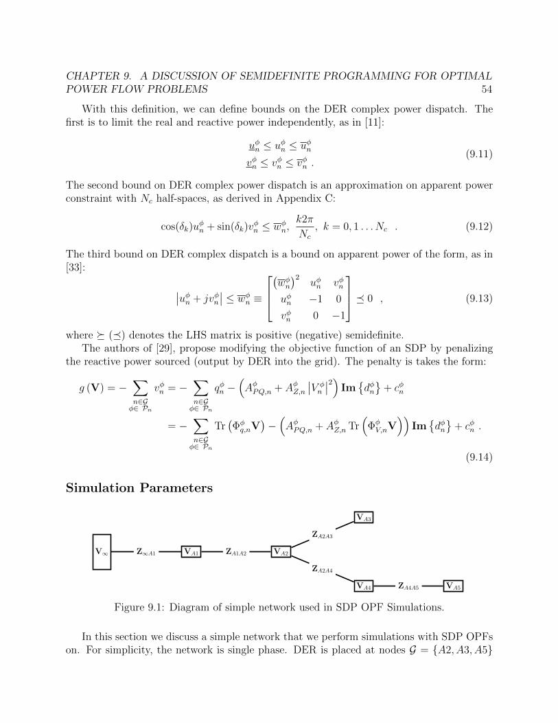
CHAPTER 9. A DISCUSSION OF SEMIDEFINITE PROGRAMMING FOR OPTIMALPOWER FLOW PROBLEMS 54
With this definition, we can define bounds on the DER complex power dispatch. Thefirst is to limit the real and reactive power independently, as in [11]:
uφn ≤ uφn ≤ uφn
vφn ≤ vφn ≤ vφn .(9.11)
The second bound on DER complex power dispatch is an approximation on apparent powerconstraint with Nc half-spaces, as derived in Appendix C:
cos(δk)uφn + sin(δk)v
φn ≤ wφn,
k2π
Nc
, k = 0, 1 . . . Nc . (9.12)
The third bound on DER complex dispatch is a bound on apparent power of the form, as in[33]:
∣∣uφn + jvφn∣∣ ≤ wφn ≡
(wφn)2
uφn vφn
uφn −1 0
vφn 0 −1
� 0 , (9.13)
where � (�) denotes the LHS matrix is positive (negative) semidefinite.The authors of [29], propose modifying the objective function of an SDP by penalizing
the reactive power sourced (output by DER into the grid). The penalty is takes the form:
g (V) = −∑n∈Gφ∈ Pn
vφn = −∑n∈Gφ∈ Pn
qφn −(AφPQ,n + AφZ,n
∣∣V φn
∣∣2) Im{dφn}
+ cφn
= −∑n∈Gφ∈ Pn
Tr(Φφq,nV
)−(AφPQ,n + AφZ,n Tr
(ΦφV,nV
))Im{dφn}
+ cφn .
(9.14)
Simulation Parameters
V∞ VA1Z∞A1 VA2ZA1A2
VA3
ZA2A3
VA4
ZA2A4
VA5ZA4A5
Figure 9.1: Diagram of simple network used in SDP OPF Simulations.
In this section we discuss a simple network that we perform simulations with SDP OPFson. For simplicity, the network is single phase. DER is placed at nodes G = {A2, A3, A5}
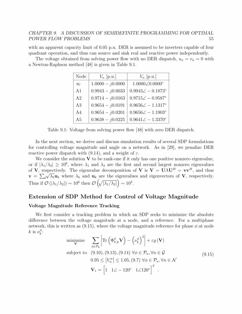
CHAPTER 9. A DISCUSSION OF SEMIDEFINITE PROGRAMMING FOR OPTIMALPOWER FLOW PROBLEMS 55
with an apparent capacity limit of 0.05 p.u. DER is assumed to be inverters capable of fourquadrant operation, and thus can source and sink real and reactive power independently.
The voltage obtained from solving power flow with no DER dispatch, un = vn = 0 witha Newton-Raphson method [48] is given in Table 9.1.
Node Vn [p.u.] Vn [p.u.]
∞ 1.0000− j0.0000 1.0000∠0.0000◦
A1 0.9943− j0.0033 0.9943∠− 0.1873◦
A2 0.9714− j0.0163 0.9715∠− 0.9587◦
A3 0.9654− j0.0191 0.9656∠− 1.1317◦
A4 0.9654− j0.0201 0.9656∠− 1.1903◦
A5 0.9638− j0.0225 0.9641∠− 1.3370◦
Table 9.1: Voltage from solving power flow [48] with zero DER dispatch.
In the next section, we derive and discuss simulation results of several SDP formulationsfor controlling voltage magnitude and angle on a network. As in [29], we penalize DERreactive power dispatch with (9.14), and a weight of ε.
We consider the solution V to be rank-one if it only has one positive nonzero eigenvalue,or if |λ1/λ2| ≥ 106, where λ1 and λ2 are the first and second largest nonzero eigenvaluesof V, respectively. The eigenvalue decomposition of V is V = UΛUH = vvH , and thusv =
∑k
√λkuk where λk and uk are the eigenvalues and eigenvectors of V, respectively.
Thus if O (|λ1/λ2|) ∼ 106 then O(√|λ1/λ2|
)∼ 103.
Extension of SDP Method for Control of Voltage Magnitude
Voltage Magnitude Reference Tracking
We first consider a tracking problem in which an SDP seeks to minimize the absolutedifference between the voltage magnitude at a node, and a reference. For a multiphasenetwork, this is written as (9.15), where the voltage magnitude reference for phase φ at nodek is νφk :
minimizeV
∑φ∈Pk
∣∣∣∣Tr(
ΦφV,kV
)−(νφk
)2∣∣∣∣+ εg (V)
subject to (9.10), (9.13), (9.14) ∀φ ∈ Pn,∀n ∈ G0.95 ≤
∣∣V φn
∣∣ ≤ 1.05, (9.7) ∀φ ∈ Pn,∀n ∈ N
V1 =[1 1∠− 120◦ 1∠120◦
]T.
(9.15)
CHAPTER 9. A DISCUSSION OF SEMIDEFINITE PROGRAMMING FOR OPTIMALPOWER FLOW PROBLEMS 56
The objective function can be transformed into a linear objective function and two linearconstraints by introducing a new variable γφV,k such that:
minimizeV,γφk
∑φ∈Pk
γφk + εg (V)
subject to (9.10), (9.13), (9.14) ∀φ ∈ Pn,∀n ∈ G0.95 ≤
∣∣V φn
∣∣ ≤ 1.05, (9.7) ∀φ ∈ Pn,∀n ∈ N
V1 =[1 1∠− 120◦ 1∠120◦
]TTr(
ΦφV,kV
)−(νφk
)2≤ γφV,k ∀φ ∈ Pk
− Tr(
ΦφV,kV
)+(νφk
)2≤ γφV,k ∀φ ∈ Pk .
(9.16)
The OPF can also be cast as a quadratic minimization, as in (9.17):
minimizeV
∑φ∈Pk
(Tr(
ΦφV,kV
)−(νφk
)2)2
+ εg (V)
subject to (9.10), (9.13), (9.14) ∀φ ∈ Pn,∀n ∈ G0.95 ≤
∣∣V φn
∣∣ ≤ 1.05, (9.7) ∀φ ∈ Pn,∀n ∈ N
V1 =[1 1∠− 120◦ 1∠120◦
]T,
(9.17)
and transformed by introducing the variable γφk and a semidefinite matrix, as in [32]:
minimizeV,γφk
∑φ∈Pk
γφk + εg (V)
subject to (9.10), (9.13), (9.14) ∀φ ∈ Pn,∀n ∈ G0.95 ≤
∣∣V φn
∣∣ ≤ 1.05, (9.7) ∀φ ∈ Pn, ∀n ∈ N
V1 =[1 1∠− 120◦ 1∠120◦
]T γφk
(Tr(
ΦφV,kV
)−(νφk
)2)(
Tr(
ΦφV,kV
)−(νφk
)2)1
� 0 ∀φ ∈ Pk .
(9.18)
Simulations were run on the network shown in Figure 9.1, with the OPF of (9.16), withthe node k = A2 given a reference. We perform simulations for voltage magnitude referencesvarying from 0.95 to 1.0 in increments of 0.005 p.u. Additionally, the DER reactive powerdispatch is penalized as in [29] with ε varying from 0 to 0.5 in increments of 0.05.
Figure 9.2 gives the results a simulation of (9.16) with varying voltage magnitude ref-erence and reactive power dispatch penalty. It can be seen that for a voltage magnitude
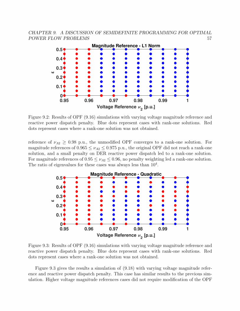
CHAPTER 9. A DISCUSSION OF SEMIDEFINITE PROGRAMMING FOR OPTIMALPOWER FLOW PROBLEMS 57
0.95 0.96 0.97 0.98 0.99 1
Voltage Reference 2 [p.u.]
0
0.1
0.2
0.3
0.4
0.5Magnitude Reference - L1 Norm
Figure 9.2: Results of OPF (9.16) simulations with varying voltage magnitude reference andreactive power dispatch penalty. Blue dots represent cases with rank-one solutions. Reddots represent cases where a rank-one solution was not obtained.
reference of νA2 ≥ 0.98 p.u., the unmodified OPF converges to a rank-one solution. Formagnitude references of 0.965 ≤ νA2 ≤ 0.975 p.u., the original OPF did not reach a rank-onesolution, and a small penalty on DER reactive power dispatch led to a rank-one solution.For magnitude references of 0.95 ≤ νA2 ≤ 0.96, no penalty weighting led a rank-one solution.The ratio of eigenvalues for these cases was always less than 104.
0.95 0.96 0.97 0.98 0.99 1
Voltage Reference 2 [p.u.]
0
0.1
0.2
0.3
0.4
0.5Magnitude Reference - Quadratic
Figure 9.3: Results of OPF (9.16) simulations with varying voltage magnitude reference andreactive power dispatch penalty. Blue dots represent cases with rank-one solutions. Reddots represent cases where a rank-one solution was not obtained.
Figure 9.3 gives the results a simulation of (9.18) with varying voltage magnitude refer-ence and reactive power dispatch penalty. This case has similar results to the previous sim-ulation. Higher voltage magnitude references cases did not require modification of the OPF

CHAPTER 9. A DISCUSSION OF SEMIDEFINITE PROGRAMMING FOR OPTIMALPOWER FLOW PROBLEMS 58
objective function. Cases where the voltage magnitude references was 0.965 ≤ νA2 ≤ 0.975p.u., required a small penalty to obtain a rank-one solution. Finally, the cases where0.95 ≤ νA2 ≤ 0.96 did not converge to a rank-one solution despite with any weightingon DER reactive power dispatch.
Minimization of Voltage Magnitude Difference
The previous OPFs can be extended to minimize the difference between voltage magni-tude across different phases at a node, between the same phase at different nodes, or betweendifferent phases at different nodes:
Eφkl =
∣∣∣V φk
∣∣∣2 − ∣∣∣V φl
∣∣∣2 = Tr(
ΦφV,kV
)− Tr
(ΦφV,lV
)= Tr
(ΦφV,klV
), (9.19)
where ΦφV,kl = Φφ
V,k −ΦφV,l. An OPF minimizing the absolute value of the difference between
voltage magnitude of phase φ at node k and node l is:
minimizeV
∑φ∈Pkl
∣∣∣Tr(
ΦφV,klV
)∣∣∣+ εg (V)
subject to (9.10), (9.13), (9.14) ∀φ ∈ Pn,∀n ∈ G0.95 ≤
∣∣V φn
∣∣ ≤ 1.05, (9.7) ∀φ ∈ Pn,∀n ∈ N
V1 =[1 1∠− 120◦ 1∠120◦
]T.
(9.20)
This objective can likewise be transformed into a linear objective function and two linearconstraints as in:
minimizeV,γφkl
∑φ∈Pkl
γφkl + εg (V)
subject to (9.10), (9.13), (9.14) ∀φ ∈ Pn,∀n ∈ G0.95 ≤
∣∣V φn
∣∣ ≤ 1.05, (9.7) ∀φ ∈ Pn,∀n ∈ N
V1 =[1 1∠− 120◦ 1∠120◦
]TTr(
ΦφV,klV
)≤ γφV,kl ∀φ ∈ Pkl
− Tr(
ΦφV,klV
)≤ γφV,kl ∀φ ∈ Pkl .
(9.21)
The OPF minimizing voltage magnitude difference can also be cast a quadratic minimization
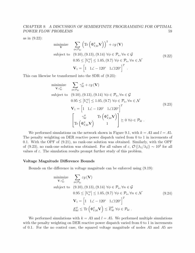
CHAPTER 9. A DISCUSSION OF SEMIDEFINITE PROGRAMMING FOR OPTIMALPOWER FLOW PROBLEMS 59
as in (9.22):
minimizeV
∑φ∈Pkl
(Tr(
ΦφV,klV
))2+ εg (V)
subject to (9.10), (9.13), (9.14) ∀φ ∈ Pn,∀n ∈ G0.95 ≤
∣∣V φn
∣∣ ≤ 1.05, (9.7) ∀φ ∈ Pn,∀n ∈ N
V1 =[1 1∠− 120◦ 1∠120◦
]T.
(9.22)
This can likewise be transformed into the SDR of (9.23):
minimizeV,γφkl
∑φ∈Pkl
γφkl + εg (V)
subject to (9.10), (9.13), (9.14) ∀φ ∈ Pn,∀n ∈ G0.95 ≤
∣∣V φn
∣∣ ≤ 1.05, (9.7) ∀φ ∈ Pn,∀n ∈ N
V1 =[1 1∠− 120◦ 1∠120◦
]T γφkl Tr
(ΦφV,klV
)Tr(
ΦφV,klV
)1
� 0 ∀φ ∈ Pkl .
(9.23)
We performed simulations on the network shown in Figure 9.1, with k = A3 and l = A5.The penalty weighting on DER reactive power dispatch varied from 0 to 1 in increments of0.1. With the OPF of (9.21), no rank-one solution was obtained. Similarly, with the OPFof (9.23), no rank-one solution was obtained. For all values of ε, O (|λ1/λ2|) ∼ 103 for allvalues of ε. The simulation results prompt further study of this problem.
Voltage Magnitude Difference Bounds
Bounds on the difference in voltage magnitude can be enforced using (9.19):
minimizeV,γφkl
∑φ∈Pkl
εg (V)
subject to (9.10), (9.13), (9.14) ∀φ ∈ Pn,∀n ∈ G0.95 ≤
∣∣V φn
∣∣ ≤ 1.05, (9.7) ∀φ ∈ Pn,∀n ∈ N
V1 =[1 1∠− 120◦ 1∠120◦
]TEφkl ≤ Tr
(ΦφV,klV
)≤ E
φ
kl ∀φ ∈ Pkl .
(9.24)
We performed simulations with k = A3 and l = A5. We performed multiple simulationswith the penalty weighting on DER reactive power dispatch varied from 0 to 1 in incrementsof 0.1. For the no control case, the squared voltage magnitude of nodes A3 and A5 are

CHAPTER 9. A DISCUSSION OF SEMIDEFINITE PROGRAMMING FOR OPTIMALPOWER FLOW PROBLEMS 60
|VA3|2 = 0.9323 and |VA5|2 = 0.9294, respectively. With a magnitude difference bound of−0.01 ≤ Eφ
kl ≤ 0.01 no rank one solution was found, and O (|λ1/λ2|) ∼ 103 for all values
of ε. With a magnitude difference bound of −0.005 ≤ Eφkl ≤ 0.005, no rank one solution
was found, and O (|λ1/λ2|) ∼ 103 for all values of ε. With a magnitude difference bound of−0.001 ≤ Eφ
kl ≤ 0.001, no rank one solution was found, and O (|λ1/λ2|) ∼ 103 for all valuesof ε. The simulation results prompt further study of this problem.
Extension of SDP Method for Control of Voltage Angle
Consider an off-diagonal index of V corresponding to the product of the phasor of aphase φ at node m and the complex conjugate of the phasor for phase φ at node n, whichcan be expressed in polar form:
V φm
(V φn
)∗=∣∣V φm
∣∣ ∣∣V φn
∣∣∠ (θπm − θπn)
=∣∣V φm
∣∣ ∣∣V φn
∣∣ [cos (θπm − θπn) + j sin (θπm − θπn)] . (9.25)
We now define θφmn = θφm− θφn. The ratio of the real and imaginary components of V φm
(V φn
)∗is defined by the tangent function:
Im{V φm
(V φn
)∗}Re{V φm
(V φn
)∗} =
∣∣V φm
∣∣ ∣∣V φn
∣∣ sin (θφmn)∣∣∣V φm
∣∣∣ ∣∣∣V φn
∣∣∣ cos(θφmn) = tan
(θφmn). (9.26)
The real and imaginary components of V φm
(V φn
)∗are defined as:
Re{V φm
(V φn
)∗}=
1
2
[V φm
(V φn
)∗+(V φm
)∗V φn
]=
1
2
[Tr(ΦφmnV
)+ Tr
(ΦφnmV
)]Im{V φm
(V φn
)∗}=
1
j2
[V φm
(V φn
)∗ − (V φm
)∗V φn
]=
1
j2
[Tr(ΦφmnV
)− Tr
(ΦφnmV
)],
(9.27)
where the matrices Φφmn and Φφ
nm are defined as:
Φφmn = eφn
(eφm)T, Φφ
nm = eφm(eφn)T
, (9.28)
using the same notation for eφm and eφn as in [11]. Thus, we can use (9.26), (9.27), and (9.28)to obtain relationships defining an off diagonal element of V in terms of the its angle:
Re{V φm
(V φn
)∗}sin(θφmn)
= Im{V φm
(V φn
)∗}cos(θφmn)
Tr(
ΦφRe,mnV
)sin(θφmn)
= Tr(
ΦφIm,mnV
)cos(θφmn)
ΦRe,mn =1
2
[Φφmn + Φφ
nm
], ΦIm,mn =
1
j2
[Φφmn − Φφ
nm
].
(9.29)
While 9.29 can be used to directly assign voltage angles, it is likely to not be practicallyapplicable as choosing a feasible set of angles may prove difficult or impossible.

CHAPTER 9. A DISCUSSION OF SEMIDEFINITE PROGRAMMING FOR OPTIMALPOWER FLOW PROBLEMS 61
Voltage Angle Difference Bounds
On the interval 〈−π/2, π/2〉, a ≤ b⇒ tan (a) ≤ tan (b), and thus we can take advantageof this property to introduce upper and lower bounds on voltage phasor angle using the
previous analysis. Defining a lower angle bound as θφmn, and an upper angle bound as θφ
mn,we can introduce a new constraint:
θφmn ≤ θφmn ≤ θφ
mn ⇒ tan(θφmn)≤ tan
(θφmn)≤ tan
(θφ
mn
), (9.30)
where θφmn, θφ
mn and θφmn are all on the interval 〈−π, π〉. With the definition of the real andimaginary parts of V φ
m
(V φn
)∗from (9.26), this can be rewritten as:
tan(θφmn)≤
Im{V φm
(V φn
)∗}Re{V φm
(V φn
)∗} ≤ tan(θφ
mn
), (9.31)
which can be rewritten by multiplying by the denominator:
tan(θφmn)Re{V φm
(V φn
)∗} ≤ Im{V φm
(V φn
)∗} ≤ tan(θφ
mn
)Re{V φm
(V φn
)∗}. (9.32)
Using the trace operator, this can be rewritten as a constraint for the voltage angle lowerbound:
tan(θφmn)
Tr(
ΦφRe,mnV
)≤ Tr
(ΦφIm,mnV
), (9.33)
and voltage angle upper bound:
Tr(
ΦφIm,mnV
)≤ tan
(θφ
mn
)Tr(
ΦφRe,mnV
). (9.34)
An example OPF that incorporates bounds on voltage angle difference is given by (9.35):
minimizeV
f (V) + εg (V)
subject to (9.10), (9.13), (9.14) ∀φ ∈ Pn,∀n ∈ G0.95 ≤
∣∣V φn
∣∣ ≤ 1.05, (9.7) ∀φ ∈ Pn,∀n ∈ N
V1 =[1 1∠− 120◦ 1∠120◦
]Ttan(θφkl
)Tr(
ΦφRe,klV
)≤ Tr
(ΦφRe,klV
)∀φ ∈ Pkl
Tr(
ΦφIm,klV
)≤ tan
(θφ
kl
)Tr(
ΦφRe,klV
)∀φ ∈ Pkl .
(9.35)
We perform simulations on the network show in Figure 9.1. The objective function of(9.35) is f (V) = |VA2|2 = Tr (ΦV,2V). We place angle bounds where k = A3 and l = A5.
With angle bounds of θφkl = −0.005 and θφ
kl = 0.005, a rank-one solution is obtained withε = 0 and O |λ1/λ2| ≈ 107. Solving power flow with the optimal DER dispatch from 9.35,
CHAPTER 9. A DISCUSSION OF SEMIDEFINITE PROGRAMMING FOR OPTIMALPOWER FLOW PROBLEMS 62
VA3 = 0.9743∠ − 1.1142◦ and VA5 = 0.9737∠ − 1.1630◦. The resultant voltage angles arewithin the imposed bounds.
With angle bounds of θφkl = −0.001 and θφ
kl = 0.001, a rank-one solution is obtained withε = 0 and O |λ1/λ2| ≈ 107. Solving power flow with the optimal DER dispatch from 9.35,VA3 = 0.9733∠ − 1.1368◦ and VA5 = 0.9724∠ − 1.1366◦. The resultant voltage angles arewithin the imposed bounds.
While simulation results are promising, the lack of success in controlling voltage magni-tude motivates the concerted analysis of controlling voltage magnitude and angle within anSDP formulation.
9.4 Conclusions
This chapter provided a discussion of the literature on SDP for OPF problems, and apreliminary study into SDP for controlling voltage magnitude and angle. While literaturehas detailed the success of SDP as a method for solving nonlinear and nonconvex OPFs,these works also highlighted drawbacks to the method. Simulation results motivate furtheranalysis.
The first part of this chapter discusses recent works on SDP OPFs that show the method’spromise, however, these works also outline why it may not be a viable method with currentsolvers. In [24], simulations have shown that a rank-one solution may not be obtainable,even for a feasible problem, when load line flow constraints are tightened. In [27], analysishas shown that too many equality constraints and binding inequality constraints will preventconvergence to a rank-one solution. In [29], to rectify convergence issues with certain cyclicnetworks, the authors suggest a possible solution of augmenting the objective function topenalize DER reactive power dispatch, thus changing the original problem. Finally, simu-lation results in [11] show that SDP convergence is sensitive to slack bus voltage. Recentliterature points to methods for addressing some of these issues with iterative methods [26,50, 51].
The second part of this chapter explores SDP as a method for solving OPFs for controllingvoltage magnitude and angle. We derive SDP formulations for several OPFs for managementof voltage magnitude and angle. Simulation results show that an OPF that tracks a voltagemagnitude target will converge to a rank-one solution for higher target values, will converge toa rank-one solution for certain target values with a penalty on DER reactive power dispatch,and will not converge to a rank-one solution for lower target vales.
A second simulation in which an OPF seeks to minimize voltage magnitude differencefailed to produce a rank-one solution, despite the OPF modification proposed in [29]. Athird simulation in which an OPF seeks to place constraints on voltage magnitude differ-ence failed to produce a rank-one solution, despite the OPF modification proposed in [29].Finally, a fourth simulation in which an OPF seeks to impose constraints on voltage angledifference successfully produced rank-one solutions for several bounds, without necessitating

CHAPTER 9. A DISCUSSION OF SEMIDEFINITE PROGRAMMING FOR OPTIMALPOWER FLOW PROBLEMS 63
the OPF modification proposed in [29]. These simulation results motivate further analysisinto controlling voltage magnitude with SDP OPFs.
This work is not an exhaustive or definitive study on the efficacy of SDP OPFs in con-trolling voltage magnitude and angle, but rather an preliminary exploration. The lack ofrank-one solutions for minimizing voltage magnitude difference, and lack of objective thatminimizes voltage angle difference motivates the need for the investigation of other powerflow models for DER optimization.

64
Chapter 10
Derivation of a Linearized UnbalancedPower Flow Model
10.1 Introduction
From the discussion of semidefinite programming presented in Chapter 9, it is clearthat SDP and current solves currently have drawbacks that may preclude its application tosolve OPF large, multiphase, or meshed (cyclic) networks. With this in in mind, we seek anovel model for unbalanced power flow model that can easily be incorporated into a convexoptimization program.
Baran and Wu developed the DistFlow single phase power flow model in [9], and asimplified version of the DistFlow model in [8]. The simplified version contains linear powerflow equations, except for the loss terms which are quadratic in real and reactive line powerflows.
The DistFlow and its linearized version, often referred to as LinDistFlow, have beenused for optimization and control of distribution network resources, along with networkstate estimation. In [12], the authors utilize a modified version of the simplified simplifiedDistFlow equations to develop local volt/var control schemes. The authors of [25] employsimplified simplified DistFlow in developing localized voltage regulation algorithms. In [10],the authors take advantage of the simplified simplified DistFlow system of equations toinvestigate linear approximations of the the power flow manifold.
The DistFlow has also been extended to three phase systems, as have the simplifiedDistFlow system of equations. Gan and Low [14] extend the DistFlow to three phases,and apply simplifying assumptions to obtain linear version of the simplified DistFlow. Theauthors conclude that for networks with small line losses and nearly balanced voltages,the linear approximation is accurate. The authors of [20] develop localized single phaseand three phase voltage control schemes using the single phase and three phase simplifiedDistFlow equations. The authors also derive a version of the three phase simplified DistFlowfor voltage regulation in[39]. The authors also derive approximations for previously omitted
CHAPTER 10. DERIVATION OF A LINEARIZED UNBALANCED POWER FLOWMODEL 65
nonlinear terms.As the simplified DistFlow and its three phase counterpart are linear, the systems of
equations can be incorporated into a linear program (LP) or quadratic program (QP), orother convex optimization programs. However, the models of [14], [20], and [39] do notcontain the voltage phasor angle. To this end, we builds upon the three phase simplifiedDistFlow by adding equations for voltage phase angle.
10.2 Derivation of Power and Losses for Unbalanced
Approximate Power Flow
We now derive complex power and loss terms on a line (m,n) ∈ E . This derivation followsthat of [14] and [39] for three phases systems. Our derivation arrives at the same result asin [14], but with different nomenclature.
Power Referenced to Line Receiving Node
We now derive complex power and losses for lines (l,m) ∈ E and (m,n) ∈ E that connectto node m ∈ N . This derivation follows that of [14] and [39] for three phases systems. Ourderivation arrives at the same result as in [14], but with different nomenclature and method.
To start, we take the HP of Vm and the complex conjugate (non-transposed) of (8.6):∑l:(l,m)∈E
Vm ◦ I∗lm = Vm ◦ i∗m +∑
n:(m,n)∈E
Vm ◦ I∗mn . (10.1)
The Vm term inside the summation on the RHS is substituted using (8.3):∑l:(l,m)∈E
Vm ◦ I∗lm = Vm ◦ i∗m +∑
n:(m,n)∈E
Vn ◦ I∗mn + (ZmnImn) ◦ I∗mn . (10.2)
Here, we define the per phase complex power as Sφlm,m = Vφm
(Iφlm
)∗, and Sφmn,n = Vφ
n
(Iφmn)∗
,
and the 3 × 1 vectors of complex power phasors Slm,m = Vm ◦ I∗lm and Smn,n = Vn ◦ I∗mnwhere Smn,n is the power from node m to node n at node n, such that:∑
l:(l,m)∈E
Slm,m = sm +∑
n:(m,n)∈E
Smn,n + Lmn . (10.3)
As we define Iφmn = 0 ∀φ /∈ Pmn and Iφmn = 0 ∀φ /∈ Pmn, then clearly Sφmn,n = 0 ∀φ /∈ Pmn.The term Lmn ∈ C3×1 is a nonlinear and non-convex loss term. Thus this equation
will be difficult to incorporate into an optimization framework. We therefore introduce thefollowing assumption:
A1: Lmn is constant ∀(m,n) ∈ E
CHAPTER 10. DERIVATION OF A LINEARIZED UNBALANCED POWER FLOWMODEL 66
Applying A1 to (10.3) gives a linear equation for the conservation of complex power at nodem ∈ N , (10.4). ∑
l:(l,m)∈E
Slm,m ≈ sm +∑
n:(m,n)∈E
Smn,n + Lmn . (10.4)
Additionally, following the analysis in [9] and [14], we introduce a second assumption:
A2: Lmn =[0 0 0
]T∀(m,n) ∈ E
Assumption A2 states that line losses are small compared to line flows, such that∣∣Lφmn∣∣�∣∣Sφmn∣∣ ∀φ ∈ Pmn ∀(m,n) ∈ E and can therefore be neglected. With this assumption applied
to (10.4), we arrive at a simplified equation for the conservation of complex power (10.5):∑l:(l,m)∈E
Slm ≈ sm +∑
n:(m,n)∈E
Smn . (10.5)
It should be noted that when A2 is applied, we will drop the second subscript denotingthe node the power is referenced at. This is because if losses are assumed to be 0, thenthe power at the transmitting node and receiving node of a line are equivalent, such thatSmn,m = Smn,n = Smn ∀(m,n) ∈ E , and Sφmn = 0 ∀φ /∈ Pmn.
Power Referenced to Line Transmitting Node
In the previous subsection, we derived three phase complex power flow for lines connectedto node m ∈ N , with the power referenced to the receiving end of the line. While thetransmitting and receiving end of a line (m,n) ∈ E can be arbitrarily chosen, referencingpower at one end or the other may improve accuracy of a model, especially when usingmeasured voltage and power values.
We now derive a similar set of equation to (10.2) – (10.5), however with line complexpower defined at the line’s transmitting node. We again start by taking the HP of Vm andthe complex conjugate (non-transposed) of (8.6):∑
l:(l,m)∈E
Vm ◦ I∗lm = Vm ◦ i∗m +∑
n:(m,n)∈E
Vm ◦ I∗mn . (10.6)
The Vm term inside the summation on the LHS is substituted using (8.3) on line (l,m) ∈ E :∑l:(l,m)∈E
Vl ◦ I∗lm − (ZlmIlm) ◦ I∗lm = Vm ◦ i∗m +∑
n:(m,n)∈E
Vm ◦ I∗mn . (10.7)
Here, we define the per phase complex power as Sφlm,l = Vφl
(Iφlm
)∗and Sφmn,m = Vφ
m
(Iφmn)∗
.
The 3×1 vector of complex power phasors are defined as Slm,l = Vl◦I∗lm and Smn,m = Vm◦I∗mnwhere Smn,m is the power from node m to node n at node m, such that:∑
l:(l,m)∈E
Slm,l − Llm = sm +∑
n:(m,n)∈E
Smn,m . (10.8)

CHAPTER 10. DERIVATION OF A LINEARIZED UNBALANCED POWER FLOWMODEL 67
As we define Iφmn = 0 ∀φ /∈ Pmn, then clearly Sφmn,m = 0 ∀φ /∈ Pmn.Similarly to (10.3), Llm ∈ C3×1 is a nonlinear and non-convex loss term. Applying A1
on line (l,m) ∈ E to (10.8) gives a linear equation for the conservation of complex power atnode m, (10.9): ∑
l:(l,m)∈E
Slm,l − Llm ≈ sm +∑
n:(m,n)∈E
Smn,m . (10.9)
Additionally, applying A2 further simplifies (10.9) into (10.10):∑l:(l,m)∈E
Slm ≈ sm +∑
n:(m,n)∈E
Smn . (10.10)
It should be noted that (10.5) and (10.10) are equivalent, as when A2 is applied to a line(m,n) ∈ E , Sφmn,m = Sφmn,n = Sφmn ∀φ ∈ Pmn and Smn,m = Smn,n = Smn when losses areneglected.
10.3 Derivation of Voltage Magnitude Relations for
Unbalanced Approximate Power Flow
In this section, we present a derivation for squared voltage magnitudes and complex mul-tiphase power for unbalanced systems. This section follows derivations in [14, 39], howeverwe present it in this work to keep a uniform nomenclature with the next section, to motivatethe extension of the model to consider voltage angles in the following section, and to high-light a common structure shared between the voltage magnitude/complex power flow andvoltage angle/complex power flow relationships.
The reader should note that here we present the derivation for a line with three phaseswhere Pmn = {a, b, c}. For lines with less than three phases (|Pmn| = 1 or |Pmn| = 2), allequations should be indexed by Pmn as (8.4) is.
As in the previous section, Section 10.2, we will derive equations relating voltage mag-nitude to complex power flow first referencing voltage and power to the receiving node of aline, then the transmitting node.
Derivation of Magnitude Equation with Voltage and PowerReferenced to Line Receiving Node
To start, we consider line (m,n) ∈ E , and take the Hadamard Product of (8.3) and itscomplex conjugate (non-transposed):
Vm ◦V∗m = (Vn + ZmnImn) ◦ (Vn + ZmnImn)∗ . (10.11)
This can be rewritten by distributing the terms on the RHS:
Vm ◦V∗m = Vn ◦V∗n + Vn ◦ (ZmnImn)∗+ (ZmnImn) ◦V∗n + (ZmnImn) ◦ (ZmnImn)∗ . (10.12)

CHAPTER 10. DERIVATION OF A LINEARIZED UNBALANCED POWER FLOWMODEL 68
Now, we define the real scalar:
Eφm =
∣∣V φm
∣∣2 = V φm(V φ
m)∗ , (10.13)
the 3× 1 real vector:
Em =[Eam Eb
m Ecm
]T= Vm ◦V∗m , (10.14)
and the 3× 1 real vector:
Hmn = (ZmnImn) ◦ (ZmnImn)∗ = (Vm −Vn) ◦ (Vm −Vn)∗ . (10.15)
With these definitions, we also take advantage of the commutative property of the HP andgroup the second and third terms of the RHS of (10.12) inside the real operator, as they arethe complex conjugate of each other:
Em = En + 2 Re {(ZmnImn)∗ ◦Vn}+ Hmn . (10.16)
We expand (ZmnImn)∗ ◦Vn to obtain:
Em = En + 2 Re
V
an
(ZaamnI
amn + Zab
mnIbmn + Zac
mnIcmn
)∗V bn
(ZbamnI
amn + Zbb
mnIbmn + Zbc
mnIcmn
)∗V cn
(ZcamnI
amn + Zcb
mnIbmn + Zcc
mnIcmn
)∗+ Hmn . (10.17)
Now, we use the definition of complex power at the receiving node where(Iφmn)∗
= Sφmn,n/Vφn ,
and define the term γφψn = V φn /V
ψn , thus expand (10.17) to (10.18):
Em = En + 2 Re
(Zaa
mn)∗Samn,n + γabn (Zabmn)∗Sbmn,n + γacn (Zac
mn)∗Scmn,n
γban (Zbamn)∗Samn,n + (Zbb
mn)∗Sbmn,n + γbcn (Zbcmn)∗Scmn,n
γcan (Zcamn)∗Samn,n + γcbn (Zcb
mn)∗Sbmn,n + (Zccmn)∗Scmn,n
+ Hmn . (10.18)
The 3 × 1 vector on the RHS can be separated into a 3 × 3 matrix multiplied by the 3 × 1vector Smn,n:
Em = En + 2 Re
(Zaa
mn)∗ γabn (Zabmn)∗ γacn (Zac
mn)∗
γban (Zbamn)∗ (Zbb
mn)∗ γbcn (Zbcmn)∗
γcan (Zcamn)∗ γcbn (Zcb
mn)∗ (Zccmn)∗
S
amn,n
Sbmn,n
Scmn,n
+ Hmn . (10.19)
Defining the matrix Γn ∈ C3×3 as:
Γn = Vn (1/Vn)T =
1 γabn γacn
γban 1 γbcn
γcan γcbn 1
, (10.20)
CHAPTER 10. DERIVATION OF A LINEARIZED UNBALANCED POWER FLOWMODEL 69
we can use the definition of the HP to separate the 3× 3 matrix into two 3× 3 matrices asin:
Em = En + 2 Re {(Γn ◦ Z∗mn) Smn,n}+ Hmn . (10.21)
Finally, we apply the real operator (Re) on the RHS, separating the complex power vectorinto its active and reactive components, Smn,n = Pmn,n + jQmn,n, to arrive at:
Em = En + 2Mmn,nPmn,n − 2Nmn,nQmn,n + Hmn
Mmn,n = Re {Γn ◦ Z∗mn}Nmn,n = Im {Γn ◦ Z∗mn} .
(10.22)
We have derived equations that govern the relationship between squared voltage mag-nitudes and complex power flow across line (m,n). This system of equations is nonlinearand nonconvex system, and therefore cannot be incorporated into a convex optimizationframework without the use of approximations or convex relaxations. However, this systemcan be linearized with the following assumptions:
A3: Hmn is constant ∀(m,n) ∈ E
A4: γφψn are constant ∀φ, ψ ∈ Pn, φ 6= ψ, ∀n ∈ N
Application of assumptions A3 and A4 to (10.23) results in a linear model that relates thesquared magnitudes of nodal voltages and complex power flows to DER injected power.
Em ≈ En + 2Mmn,nPmn,n − 2Nmn,nQmn,n + Hmn . (10.23)
The magnitude equations can be further simplified via logical choices for the constantparameters of A3 and A4. Following the analysis presented in [9], we choose Hmn =[0 0 0
]T∀(m,n) ∈ E . As in [14] and [39], we assign the γφψn such that:
γabn = α γbcn = α γacn = α2
γban = α2 γcbn = α2 γcan = α∀n ∈ N ≡ Γn =
1 α α2
α2 1 α
α α2 1
∀n ∈ N , (10.24)
where α = 1∠120◦ = 12(−1 + j
√3) and α2 = α−1 = α∗ = 1∠240◦.
With these choices for Hmn and γφψn , we obtain a linear system of equations relation thedifference in voltage magnitude across line (m,n) to real and reactive power flows on theline:
Em ≈ En + 2MmnPmn,n − 2NmnQmn,n , (10.25)
Mmn =1
2
2raamn −rabmn +√
3xabmn −racmn −√
3xacmn
−rbamn −√
3xbamn 2rbbmn −rbcmn +√
3xbcmn
−rcamn +√
3xcamn −rcbmn −√
3xcbmn 2rccmn
, (10.26)
CHAPTER 10. DERIVATION OF A LINEARIZED UNBALANCED POWER FLOWMODEL 70
Nmn =1
2
−2xaamn xabmn +√
3rabmn xacmn −√
3racmn
xbamn −√
3rbamn −2xbbmn xbc +√
3rbcmn
xcamn +√
3rcamn xcbmn −√
3rcbmn −2xccmn
. (10.27)
Magnitude Equation Reference to Line Transmitting Node
Similar to Section 10.2, the magnitude equations can be rederived to reference nodevoltages at the transmitting end of the line.
To start, consider line (m,n) ∈ E with the voltage difference due to line impedance takenon the left side. We then take the Hadamard Product of (8.3) and its complex conjugate(non-transposed):
(Vm − ZmnImn) ◦ (Vm − ZmnImn)∗ = Vn ◦V∗n . (10.28)
This can be rewritten by distributing the terms on the LHS:
Vm ◦V∗m−Vm ◦ (ZmnImn)∗− (ZmnImn) ◦V∗m + (ZmnImn) ◦ (ZmnImn)∗ = Vn ◦V∗n . (10.29)
With the definitions of Em, En, Hmn, we again take advantage of the commutative propertyof the HP and group the second and third terms of the LHS of (10.29) inside the realoperator:
Em − 2 Re {(ZmnImn)∗ ◦Vm}+ Hmn = En . (10.30)
At this point, we will focus on the terms inside the real operator (Re) and expand(ZmnImn)∗ ◦Vm to obtain:
Em − 2 Re
V
am
(ZaamnI
amn + Zab
mnIbmn + Zac
mnIcmn
)∗V bm
(ZbamnI
amn + Zbb
mnIbmn + Zbc
mnIcmn
)∗V cm
(ZcamnI
amn + Zcb
mnIbmn + Zcc
mnIcmn
)∗+ Hmn = En . (10.31)
Now, we use the definition of complex power at the line transmitting node, where(Iφmn)∗
=Sφmn/V
φm, and define the term γφψm = V φ
m/Vψm , thus expand (10.31) to (10.32):
Em−2 Re
(Zaa
mn)∗Samn,m + γabm (Zabmn)∗Sbmn,m + γacm (Zac
mn)∗Scmn,m
γbam (Zbamn)∗Samn,m + (Zbb
mn)∗Sbmn,m + γbcm(Zbcmn)∗Scmn,m
γcam (Zcamn)∗Samn,m + γcbm(Zcb
mn)∗Sbmn,m + (Zccmn)∗Scmn,m
+Hmn = En . (10.32)
The 3 × 1 vector on the RHS can be separated into a 3 × 3 matrix multiplied by the 3 × 1vector Smn.
Em − 2 Re
(Zaa
mn)∗ γabm (Zabmn)∗ γacm (Zac
mn)∗
γbam (Zbamn)∗ (Zbb
mn)∗ γbcm(Zbcmn)∗
γcam (Zcamn)∗ γcbm(Zcb
mn)∗ (Zccmn)∗
S
amn,m
Sbmn,m
Scmn,m
+ Hmn = En . (10.33)

CHAPTER 10. DERIVATION OF A LINEARIZED UNBALANCED POWER FLOWMODEL 71
With the definition of Γm ∈ C3×3 as Γm = Vm (1/Vm)T , we can use the definition of the HPto separate the 3× 3 matrix into two 3× 3 matrices as in:
Em − 2 Re {(Γm ◦ Z∗mn) Smn,m}+ Hmn = En . (10.34)
Finally, we apply the real operator on the LHS, separating the complex power vector intoits active and reactive components, Smn,m = Pmn,m + jQmn,m, to arrive at:
Em = En + 2Mmn,mPmn,m − 2Nmn,mQmn,m −Hmn
Mmn,m = Re {Γm ◦ Z∗mn}Nmn,m = Im {Γm ◦ Z∗mn} .
(10.35)
It is interesting to note, at this point, that (10.22) and (10.35) are quite similar, with thedifference being that (10.22) has the matrix Γn and line powers Smn,n defined at node n andthe higher order term Hmn positive on the RHS, while (10.35) has the matrix Γm and linepowers Smn,m defined at node m and the higher order term Hmn negative on the RHS.
As with the previously derived magnitude equations with power and voltage referredto the receiving node, these equations are nonlinear and nonconvex, and we employ theassumptions A3 and A4 in the same manner. Application of assumptions A3 and A4 to(10.35) results in a linear model that relates the squared magnitudes of nodal voltages andcomplex power flows to DER injected power.
Em ≈ En + 2Mmn,mPmn,m − 2Nmn,mQmn,m −Hmn . (10.36)
Similar to the previous derivation, choosing Hmn =[0 0 0
]T∀(m,n) ∈ E , and γφψ such
that:
γabm = α γbcm = α γacm = α2
γbam = α2 γcbm = α2 γcam = α∀m ∈ N ≡ Γm =
1 α α2
α2 1 α
α α2 1
∀m ∈ N , (10.37)
we arrive at a linearized relation between voltage magnitude and complex power:
Em ≈ En + 2MmnPmn,m − 2NmnQmn,m , (10.38)
with Mmn and Nmn defined by (10.26) and (10.27), respectively.
10.4 Derivation of Voltage Angle Relations for
Unbalanced Approximate Power Flow
We now derive an extension of the power and magnitude system that relates differencesin voltage angles between adjacent nodes to complex power flows. This derivation sharesmany similarities with the analysis of Section 10.3. The derivation presented here representsa three phase line, Pmn = {a, b, c}. For lines with less than three phases (|Pmn| = 1 or|Pmn| = 2), all equations should be indexed by Pmn as (8.4) is.
This work adds to that of [14] and [39] by adding an equation for voltage angle.

CHAPTER 10. DERIVATION OF A LINEARIZED UNBALANCED POWER FLOWMODEL 72
Motivational Example
Consider a line (m,n) ∈ E . For simplicity, we assume the line is single phase, andtherefore omit the phase superscript φ. The power across (m,n) at node m is:
Smn,m = VmI∗mn = Vm (Vm − Vn)∗ /Z∗mn .
Multiplying the numerator and denominator the impedance of the line Zmn:
Smn,m = |Vm|2 Zmn/ |Zmn|2 − VmV ∗nZmn/ |Zmn|2 .
For simplicity, we will assume that |Zmn| = 1, and expand the terms of previous equationinto their respective complex components:
Smn,m = |Vm|2 (rmn + jxmn)− |Vm| |Vn| (cos (θm − θn) + j sin (θm − θn)) (rmn + jxmn) .
Grouping the real and reactive power components:
Smn,m = |Vm|2 rmn − |Vm| |Vn| (rmn cos (θm − θn)− xmn sin (θm − θn)) . . .
+ j(|Vm|2 xmn − |Vm| |Vn| (xmn cos (θm − θn) + rmn sin (θm − θn))
).
At this point, it is clear that power flow across the line (m,n) is dependent on the boththe difference in voltage magnitude between node m and n, but also the difference in voltageangle between node m and n. To further illustrate the dependence on voltage angle, weassume that the voltage magnitude at node m and node n are equal such that |Vm| = |Vn|:
Smn,m = |Vm|2 (rmn − rmn cos (θm − θn) + xmn sin (θm − θn)) . . .
+ j |Vm|2 (xmn − xmn cos (θm − θn)− rmn sin (θm − θn)) .
From this equation, it is clear that differences in voltage angle between the two node m andn will cause power to flow on (m,n). The power and magnitude equations presented in thiswork, [14], and [39], and the SDP formulation in [11], are suited to control the real andreactive power flow on lines of a distibution network.
However, these formulations are not suited to the scenario of closing a switch between twonodes, where power will begin to flow on the newly created line. With the switch open, thenodes are disconnected, and no power flows, and therefore power flow cannot be controlled.
We seek to build upon the approximate unbalanced power flow model to allow for controlof voltage angle, such that control of the complete phasor is possible. Such control will enable“cleaner” switching actions wherein a minimal voltage difference across an open switch willprevent otherwise large, and potentially equipment damaging or dangerous, power surges.
CHAPTER 10. DERIVATION OF A LINEARIZED UNBALANCED POWER FLOWMODEL 73
Angle Equations with Voltage and Power Referenced to LineReceiving Node
We begin by taking the HP of the complex conjugate of (8.3) and Vn:
V∗m ◦Vn = V∗n ◦Vn + (ZmnImn)∗ ◦Vn . (10.39)
With the results from the Section 10.3, we can substitute both terms on the RHS, andexpand the LHS with the polar representations of voltage phasors: |V
am| |V a
n |∠ (−θam + θan)∣∣V bm
∣∣ ∣∣V bn
∣∣∠ (−θbm + θbn)
|V cm| |V c
n |∠ (−θcm + θcn)
= En + (Γn ◦ Z∗mn) Smn,n . (10.40)
To be consistent with convention in the power and magnitude equations, we multiply bothsides by −1. We then take the imaginary component of both sides: |V
am| |V a
n | sin (θam − θan)∣∣V bm
∣∣ ∣∣V bn
∣∣ sin (θbm − θbn)|V cm| |V c
n | sin (θcm − θcn)
= − Im {(Γn ◦ Z∗mn) Smn,n} . (10.41)
Finally, we apply the imaginary operator to the RHS of (10.41): |Vam| |V a
n | sin (θam − θan)∣∣V bm
∣∣ ∣∣V bn
∣∣ sin (θbm − θbn)|V cm| |V c
n | sin (θcm − θcn)
= −Nmn,nPmn,n −Mmn,nQmn,n , (10.42)
with Mmn,n and Nmn,n defined as in (10.23).Inspection of the voltage angle equation reveals some interesting properties compared to
the voltage magnitude equations of (10.22). The RHS of Eqs. (10.22) and (10.42) are thereal and imaginary parts of the same argument (except for a scaling factor of one-half).
The angle equation (10.42) is nonlinear and nonconvex, and therefore difficult to incor-porate into an OPF. Therefore, we introduce the following three assumptions:
A4: γφψn are constant ∀φ, ψ ∈ Pn, φ 6= ψ, ∀n ∈ N
A5:∣∣Vφ
m
∣∣ and∣∣Vφ
n
∣∣ are constant ∀φ ∈ Pmn, ∀(m,n) ∈ N
A6: sin(θφm − θφn
)≈ θφm − θφn, via small angle approximation, ∀φ ∈ Pmn, ∀(m,n) ∈ E
It should be noted that A4 is the same as in Section 10.3, and is applied to both themagnitude and angle equations. Furthermore, the reader should note that A5 is only applied
to (10.42). We now define∣∣V φn
∣∣ = eφn ∀φ ∈ Pn ∀n ∈ N with en =[ean ebn ecn
]T∀n ∈ N as
CHAPTER 10. DERIVATION OF A LINEARIZED UNBALANCED POWER FLOWMODEL 74
a set of fixed voltage magnitude references, assumed to be constant despite control action.Application of A4, A5, and A6 to (10.42), gives a linear version of (10.42):
em ◦ en ◦Θm ≈ em ◦ en ◦Θn −Nmn,nPmn,n −Mmn,nQmn,n , (10.43)
where Θm =[θam θbm θcm
]T. This linear equation can further be simplified by selecting γφψn
as in (10.24) so that Mmn and Nmn are defined as in (10.26) and (10.27), respectively:
em ◦ en ◦Θm ≈ em ◦ en ◦Θn −NmnPmn,n −MmnQmn,n . (10.44)
Should the network voltage magnitudes be unknown or unmeasurable, they can be assumedto be that of the typical substation nominal voltage magnitude of 1, thus (10.44) becomes(10.45):
Θm ≈ Θn −NmnPmn,n −MmnQmn,n . (10.45)
Angle Equations with Voltage Referenced to Line TransmittingNode
Similar the previous two sections, we can rederive the angle equation by referencing thevoltage ratios γ and power to the transmitting node of the line. We start with by taking theHP of Vm and the complex conjugate (non-transposed) of KVL on line (m,n):
V∗m ◦Vm = V∗n ◦Vm + (ZmnImn) ◦Vm . (10.46)
With the definitions of the power and magnitude equation derivations, we rearrange bothsides:
Em =
|Vam| |V a
n |∠ (θam − θan)∣∣V bm
∣∣ ∣∣V bn
∣∣∠ (θbm − θbn)|V cm| |V c
n |∠ (θcm − θcn)
+ (Γm ◦ Z∗mn) Smn,m . (10.47)
Taking the imaginary components of both sides eliminates the LHS:
0 =
|Vam| |V a
n | sin (θam − θan)∣∣V bm
∣∣ ∣∣V bn
∣∣ sin (θbm − θbn)|V cm| |V c
n | sin (θcm − θcn)
+ Im {(Γm ◦ Z∗mn) Smn,m} . (10.48)
Applying the Im operator and subtracting the second term from both sides leads to anequation similar to that of (10.49): |V
am| |V a
n | sin (θam − θan)∣∣V bm
∣∣ ∣∣V bn
∣∣ sin (θbm − θbn)|V cm| |V c
n | sin (θcm − θcn)
= −Nmn,mPmn,m −Mmn,mQmn,m . (10.49)
CHAPTER 10. DERIVATION OF A LINEARIZED UNBALANCED POWER FLOWMODEL 75
Applying A4, A5, and A6 to (10.49) gives (10.50):
em ◦ en ◦Θm ≈ em ◦ en ◦Θn −Nmn,mPmn,m −Mmn,mQmn,m . (10.50)
This linear equation can further be simplified by selecting γφψn as in (10.24) so that Mmn
and Nmn are defined as in (10.26) and (10.27), respectively:
em ◦ en ◦Θm ≈ em ◦ en ◦Θn −NmnPmn,m −MmnQmn,m . (10.51)
If the voltage magnitudes are unknown, 10.44 can be simplified by assuming all voltagemagnitudes are roughly 1, giving 10.52:
Θm ≈ Θn −NmnPmn,m −MmnQmn,m . (10.52)
10.5 Linearized Unbalanced Power Flow Model
We now present a set of equations comprising a LUPFM for multiphase radial and meshnetworks.
In the previous sections, we have derived am equation for unbalanced multiphase powerflow, equations relating voltage magnitude to complex unbalanced power flow, and equationsrelating voltage angle to complex unbalanced power flow. For each of these, linearizingassumptions were applied only to the respective equations, without considering the otherequations. We now apply assumptions to all three equations to obtain a comprehensive andlinear appoximate power flow model.
The first equation is for a complex load on phase φ at node n, where AφPQ,n + AφZ,n =
1 ∀φ ∈ Pn, ∀n ∈ N and AφI,n = 0 ∀φ ∈ Pn, ∀n ∈ N :
sφn(V φn
)=(AφPQ,n + AφZ,nE
φn
)dφn + wφn − jcφn
sn (Vn) = (APQ,n + AZ,n ◦ En) ◦ dn + wn − jcn .(10.53)
A2 is applied to the power equation, such that:
Smn,m = Smn,n = Smn ∀(m,n) ∈ E∑l:(l,m)∈E
Slm ≈ sm +∑
n:(m,n)∈E
Smn . (10.54)
A3 is applied to the magnitude equation where Hmn =[0 0 0
]T∀(m,n) ∈ E , and A4
is applied with Γm = Γn = Γ according to (10.24), such that:
Em ≈ En + 2MmnPmn − 2NmnQmn , (10.55)
with Mmn and Nmn and defined as in (10.58).
CHAPTER 10. DERIVATION OF A LINEARIZED UNBALANCED POWER FLOWMODEL 76
A4 with Γm = Γn = Γ according to (10.24), A5, and A6 are applied to the angleequation, such that:
em ◦ en ◦Θm ≈ em ◦ en ◦Θn −NmnPmn −MmnQmn . (10.56)
with Mmn and Nmn and defined as in (10.58) Finally, if no fixed voltage references are chosenor available, they can be assigned as 1, such that eφn = 1 ∀φ ∈ Pn ∀n ∈ N :
Θm ≈ Θn −NmnPmn −MmnQmn . (10.57)
with Mmn and Nmn and defined as in (10.58):
Mmn =1
2
2raamn −rabmn +√
3xabmn −racmn −√
3xacmn
−rbamn −√
3xbamn 2rbbmn −rbcmn +√
3xbcmn
−rcamn +√
3xcamn −rcbmn −√
3xcbmn 2rccmn
Nmn =1
2
−2xaamn xabmn +√
3rabmn xacmn −√
3racmn
xbamn −√
3rbamn −2xbbmn xbc +√
3rbcmn
xcamn +√
3rcamn xcbmn −√
3rcbmn −2xccmn
.
(10.58)
The linear model presented in this section assumes three phase nodes and lines. For lineswith Pmn 6= {a, b, c}, (10.55), (10.56), (10.57), and (10.58) should be indexed as describedin Section 8.1.
77
Chapter 11
Accuracy Analysis of LinearizedUnbalanced Power FlowApproximation
The LUPFM contains several linearizing assumptions with selection of nominal param-eters, thus investigation into the accuracy of these approximations is warranted. Such ananalysis can give insight into not only the accuracy of the assumptions, but also under whatconditions the assumptions fail to reflect actual power flow.
To investigate this accuracy, we perform a Monte Carlo simulation on a modified versionof the IEEE 13 node test feeder [18], the topology of which can be seen in 11.1. In this version,the voltage regulator between nodes 650 and 632 is omitted, the transformer between nodes633 and 634 is replaced by a line of configuration 601 and length of 50 feet, and the switchbetween node 671 and 692 is replaced by a line with configuration 601 and length of 50 feet.A node representing a transmission line is appended to the network, connecting to node
650, with a fixed voltage reference of[1 1∠240◦ 1∠120◦
]T. This node is treated as an
infinite bus such that connection with the distribution network does not affect transmissionline voltage. Node phases are given in Table A.6, and line phases and per-unit impedancesare given in Table A.7.
Node are assigned complex power demands with the real, and reactive, demand com-ponents randomly chosen from uniform distribution between 0 and a maximum real, andreactive demand, respectively. The maximum component demands are independently in-creased in increments of 0.01 p.u. from 0.01 p.u. to 0.15 p.u. At each combination ofmaximum real and reactive demand, 25 simulations are conducted. At each simulation, basepower flow is solved using a Newton-Raphson method comprising the load model (8.8), KVL(8.4), and KCL (8.6), adapted from [48]. Approximate power flow is solved with a Newton-Raphson method of the LUPFM comprised of (10.53), (10.54), (10.55), (10.58), and either(10.56) or (10.57).
To explore the effect of using fixed known or measured voltage magnitudes values in the
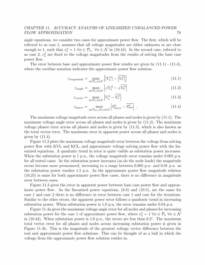
CHAPTER 11. ACCURACY ANALYSIS OF LINEARIZED UNBALANCED POWERFLOW APPROXIMATION 78
angle equations, we consider two cases for approximate power flow. The first, which will bereferred to as case 1, assumes that all voltage magnitudes are either unknown or are closeenough to 1, such that eφn = 1 ∀φ ∈ Pn, ∀n ∈ N in (10.44). In the second case, referred toas case 2, eφn are fixed to the voltage magnitudes from the results of solving the base casepower flow.
The error between base and approximate power flow results are given by (11.1) - (11.4),where the overline notation indicates the approximate power flow solution.
εmagnitude = maxφ∈Pn,n∈N
∣∣∣∣∣V φn
∣∣− ∣∣∣V φn
∣∣∣∣∣∣ (11.1)
εangle = maxφ∈Pn,n∈N
∣∣∣∠V φn − ∠V φ
n
∣∣∣ (11.2)
εvector = maxφ∈Pn,n∈N
∣∣∣V φn − V
φn
∣∣∣ (11.3)
εpower = maxφ∈Pmn,(m,n)∈E
∣∣∣Sφmn,n − Sφmn∣∣∣ . (11.4)
The maximum voltage magnitude error across all phases and nodes is given by (11.1). Themaximum voltage angle error across all phases and nodes is given by (11.2). The maximumvoltage phasor error across all phases and nodes is given by (11.3), which is also known asthe total vector error. The maximum error in apparent power across all phases and nodes isgiven by (11.4).
Figure 11.2 plots the maximum voltage magnitude error between the voltage from solvingpower flow with KVL and KCL, and approximate voltage solving power flow with the lin-earized equations. A quadratic trend in error is quite visible as substation power increases.When the substation power is 1 p.u., the voltage magnitude error remains under 0.005 p.u.for all tested cases. As the substation power increases (as do the node loads) the magnitudeerrors become more pronounced, increasing to a range between 0.005 p.u. and 0.01 p.u. asthe substation power reaches 1.5 p.u. As the approximate power flow magnitude relation(10.25) is same for both approximate power flow cases, there is no difference in magnitudeerror between cases.
Figure 11.3 gives the error in apparent power between base case power flow and approx-imate power flow. As the linearized power equations, (8.8) and (10.5), are the same forcase 1 and case 2 there is no difference in error between case 1 and case for the iterations.Similar to the other errors, the apparent power error follows a quadratic trend in increasingsubstation power. When substation power is 1.0 p.u, the error remains under 0.04 p.u.
Figure 11.4a gives the maximum voltage angle error for all nodes and phases for increasingsubstation power for the case 1 of approximate power flow, where eφn = 1 ∀φ ∈ Pn ∀n ∈ Nin (10.44). When substation power is 1.0 p.u., the errors are less than 0.2◦. The maximumtotal vector error for all phases and nodes across increasing substation power is given inFigure 11.4b. This is the magnitude of the greatest voltage vector difference between thereal and approximate power flow solutions. This can be thought of as a ball in which thevoltage from the approximate power flow solution resides in.
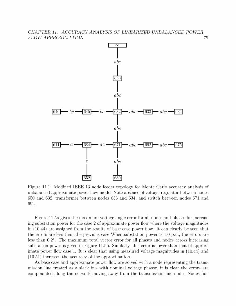
CHAPTER 11. ACCURACY ANALYSIS OF LINEARIZED UNBALANCED POWERFLOW APPROXIMATION 79
∞
650
abc
632
abc
633abc 634abc645 bc646 bc
671
abc
692abc 675abc
680
abc
684 ac
652
c
611 a
Figure 11.1: Modified IEEE 13 node feeder topology for Monte Carlo accuracy analysis ofunbalanced approximate power flow mode. Note absence of voltage regulator between nodes650 and 632, transformer between nodes 633 and 634, and switch between nodes 671 and692.
Figure 11.5a gives the maximum voltage angle error for all nodes and phases for increas-ing substation power for the case 2 of approximate power flow where the voltage magnitudesin (10.44) are assigned from the results of base case power flow. It can clearly be seen thatthe errors are less than the previous case When substation power is 1.0 p.u., the errors areless than 0.2◦. The maximum total vector error for all phases and nodes across increasingsubstation power is given in Figure 11.5b. Similarly, this error is lower than that of approx-imate power flow case 1. It is clear that using measured voltage magnitudes in (10.44) and(10.51) increases the accuracy of the approximation.
As base case and approximate power flow are solved with a node representing the trans-mission line treated as a slack bus with nominal voltage phasor, it is clear the errors arecompounded along the network moving away from the transmission line node. Nodes fur-
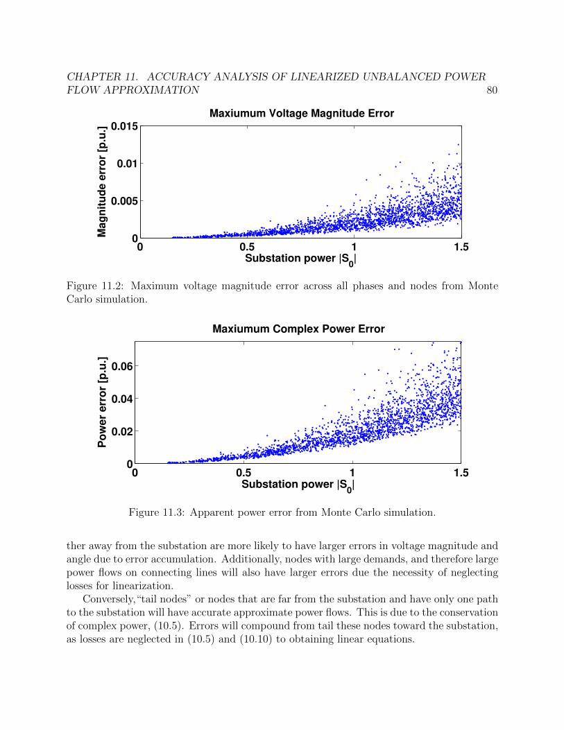
CHAPTER 11. ACCURACY ANALYSIS OF LINEARIZED UNBALANCED POWERFLOW APPROXIMATION 80
0 0.5 1 1.50
0.005
0.01
0.015
Maxiumum Voltage Magnitude Error
Substation power |S0|
Mag
nit
ud
e e
rro
r [p
.u.]
Figure 11.2: Maximum voltage magnitude error across all phases and nodes from MonteCarlo simulation.
0 0.5 1 1.50
0.02
0.04
0.06
Maxiumum Complex Power Error
Substation power |S0|
Po
we
r e
rro
r [p
.u.]
Figure 11.3: Apparent power error from Monte Carlo simulation.
ther away from the substation are more likely to have larger errors in voltage magnitude andangle due to error accumulation. Additionally, nodes with large demands, and therefore largepower flows on connecting lines will also have larger errors due the necessity of neglectinglosses for linearization.
Conversely,“tail nodes” or nodes that are far from the substation and have only one pathto the substation will have accurate approximate power flows. This is due to the conservationof complex power, (10.5). Errors will compound from tail these nodes toward the substation,as losses are neglected in (10.5) and (10.10) to obtaining linear equations.
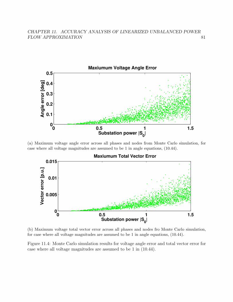
CHAPTER 11. ACCURACY ANALYSIS OF LINEARIZED UNBALANCED POWERFLOW APPROXIMATION 81
0 0.5 1 1.50
0.1
0.2
0.3
0.4
0.5
Maxiumum Voltage Angle Error
Substation power |S0|
An
gle
err
or
[deg
]
(a) Maximum voltage angle error across all phases and nodes from Monte Carlo simulation, forcase where all voltage magnitudes are assumed to be 1 in angle equations, (10.44).
0 0.5 1 1.50
0.005
0.01
0.015
Maxiumum Total Vector Error
Substation power |S0|
Vecto
r err
or
[p.u
.]
(b) Maximum voltage total vector error across all phases and nodes fro Monte Carlo simulation,for case where all voltage magnitudes are assumed to be 1 in angle equations, (10.44).
Figure 11.4: Monte Carlo simulation results for voltage angle error and total vector error forcase where all voltage magnitudes are assumed to be 1 in (10.44).
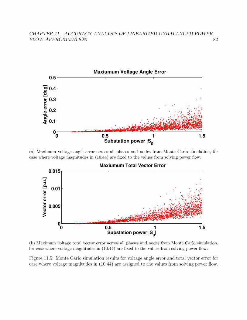
CHAPTER 11. ACCURACY ANALYSIS OF LINEARIZED UNBALANCED POWERFLOW APPROXIMATION 82
0 0.5 1 1.50
0.1
0.2
0.3
0.4
0.5
Maxiumum Voltage Angle Error
Substation power |S0|
An
gle
err
or
[deg
]
(a) Maximum voltage angle error across all phases and nodes from Monte Carlo simulation, forcase where voltage magnitudes in (10.44) are fixed to the values from solving power flow.
0 0.5 1 1.50
0.005
0.01
0.015
Maxiumum Total Vector Error
Substation power |S0|
Vecto
r err
or
[p.u
.]
(b) Maximum voltage total vector error across all phases and nodes from Monte Carlo simulation,for case where voltage magnitudes in (10.44) are fixed to the values from solving power flow.
Figure 11.5: Monte Carlo simulation results for voltage angle error and total vector error forcase where voltage magnitudes in (10.44) are assigned to the values from solving power flow.
83
Chapter 12
Applications of the LinearizedUnbalanced Power Flow Model
Control and optimization of DER on balanced networks is a topic that has encompassedmuch research effort. In recent years, these efforts have been extended to multiphase un-balanced networks, presenting new challenges in mathematical modeling and application ofoptimization techniques. In this chapter, we discuss two applications of the equations forLUPFM for optimal control of DER on distribution networks.
12.1 Voltage Magnitude Balancing
In this section, we discuss an experiment in which we incorporate linearized power, mag-nitude, and angle equations in an OPF that controls DERs to regulate and balance voltagemagnitudes on an unbalanced radial distribution network. Voltage balancing is an impor-tant objective as many three phase loads (induction motors for instance) are sensitive tohigh levels of imbalance. Furthermore, many 3-phase voltage regulation equipment actuatesbased solely on single phase measurements. Therefore, significant levels of imbalance canlead to improper operation of these devices.
The goal of this experiment is to minimize the total voltage magnitude imbalance acrossthe feeder. Voltage magnitude imbalance is defined as the absolute error of the difference ofvoltage magnitude between two difference phases at a node. The voltage imbalance at noden is defined as:
Υn =∑
φ∈Pn,ψ∈Pnφ 6=ψ
∣∣∣∣V φn
∣∣− ∣∣V ψn
∣∣∣∣ . (12.1)
For nodes with one phase (|Pn| = 1) Υn = 0 The total network voltage magnitude imbalanceis define as:
ΥN =∑n∈N
∑φ∈Pn,ψ∈Pn
φ 6=ψ
∣∣∣∣V φn
∣∣− ∣∣V ψn
∣∣∣∣ . (12.2)
CHAPTER 12. APPLICATIONS OF THE LINEARIZED UNBALANCED POWERFLOW MODEL 84
We design an OPF to minimize network voltage magnitude imbalance, regulate systemvoltage magnitude to within acceptable limits. The OPF also account for DER apparentpower constraints and regulates the dispatch. This OPF, (12.3) is:
minimizeuφn,v
φn,E
φn ,P
φmn,Q
φmn
∑n∈N
∑φ∈Pn,ψ∈Pn
φ 6=ψ
(Eφn − Eψ
n
)2+
[∑φ∈Pn
ρw∣∣wφn∣∣2
]
subject to (10.53), (10.54), (10.55), (10.58), (10.56)
Eφn ≤ Eφ
n ≤ Eφ
n ∀φ ∈ Pn, ∀n ∈ N∣∣wφn∣∣ ≤ wφn ∀φ ∈ Pn, ∀n ∈ N .
(12.3)
In 12.3, the DER dispatch apparent power constraints,∣∣wφn∣∣ ≤ w ∀φ ∈ Pn, ∀n ∈ N can
be approximated by a series of linear equations as derived in Appendix C, such that (12.3)is a true quadratic program.
It should be noted that comparison of either case to an SDP formulation of (12.3) wewere not able to obtain a rank-one solution to an equivalent problem formulated as an SDP.
Voltage Magnitude Balance Experiment on a Radial Network
We perform this experiment on a modified version of the IEEE 13 node test feeder [18],the topology of which can be seen in 12.1. In this version, the voltage regulator betweennodes 650 and 632 is omitted, the transformer between nodes 633 and 634 is replaced bya line of configuration 601 and length of 50 feet, and the switch between node 671 and692 is replaced by a line with configuration 601 and length of 50 feet.Additionally, a noderepresenting a transmission line is appended to the network, connecting to node 650, with
a fixed voltage reference of[1 1∠240◦ 1∠120◦
]T. This node is treated as an infinite bus
such that connection with the distribution network does not affect transmission line voltage.A transformer is placed between node 650 and the transmission line, with impedance asspecified in [18]. Node parameters and phases can be found in Table A.6. Line parameters,phases and impedances can be found in Table A.7.
All capacitors, listed in Table A.9, are omitted. Node demands, listed in Table A.8, arespecified by [18], are multiplied by a factor of 1.125, and are assumed to follow the model of(8.8) with AφPQ,n = 0.85, AφI,n = 0, and AφZ,n = 0.15 ∀φ ∈ Pn ∀n ∈ N .
DER are placed on all existing phases of nodes 632, 675, 680, and 684. DER are assumedto be single phase inverters capable of four quadrant operation, where the dispatch of onephase is independent of others at the same node. The DER have an apparent power limit of0.025 p.u., or 125 kW. DER placement, phases and apparent power capacity can be foundin Table A.10. The penalty on DER dispatch is weighted with ρw = 0.5. Voltage magnitude
bounds were 0.95 <=∣∣V φn
∣∣ ≤ 1.05 such that Eφn = 0.9025 and E
φ
n = 1.1025.
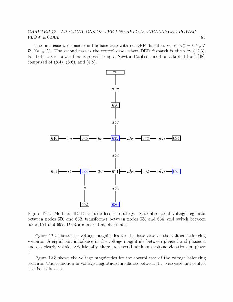
CHAPTER 12. APPLICATIONS OF THE LINEARIZED UNBALANCED POWERFLOW MODEL 85
The first case we consider is the base case with no DER dispatch, where wφn = 0 ∀φ ∈Pn ∀n ∈ N . The second case is the control case, where DER dispatch is given by (12.3).For both cases, power flow is solved using a Newton-Raphson method adapted from [48],comprised of (8.4), (8.6), and (8.8).
∞
650
abc
632
abc
633abc 634abc645 bc646 bc
671
abc
692abc 675abc
680
abc
684 ac
652
c
611 a
Figure 12.1: Modified IEEE 13 node feeder topology. Note absence of voltage regulatorbetween nodes 650 and 632, transformer between nodes 633 and 634, and switch betweennodes 671 and 692. DER are present at blue nodes.
Figure 12.2 shows the voltage magnitudes for the base case of the voltage balancingscenario. A significant imbalance in the voltage magnitude between phase b and phases aand c is clearly visible. Additionally, there are several minimum voltage violations on phasec.
Figure 12.3 shows the voltage magnitudes for the control case of the voltage balancingscenario. The reduction in voltage magnitude imbalance between the base case and controlcase is easily seen.
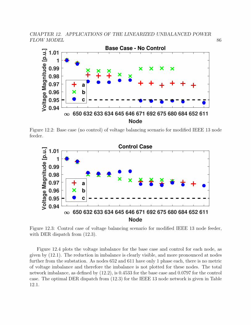
CHAPTER 12. APPLICATIONS OF THE LINEARIZED UNBALANCED POWERFLOW MODEL 86
650 632 633 634 645 646 671 692 675 680 684 652 611
Node
0.94
0.95
0.96
0.97
0.98
0.99
1
1.01
Vo
ltag
e M
ag
nit
ud
e [
p.u
.] Base Case - No Control
a
b
c
Figure 12.2: Base case (no control) of voltage balancing scenario for modified IEEE 13 nodefeeder.
650 632 633 634 645 646 671 692 675 680 684 652 611
Node
0.94
0.95
0.96
0.97
0.98
0.99
1
1.01
Vo
ltag
e M
ag
nit
ud
e [
p.u
.] Control Case
a
b
c
Figure 12.3: Control case of voltage balancing scenario for modified IEEE 13 node feeder,with DER dispatch from (12.3).
Figure 12.4 plots the voltage imbalance for the base case and control for each node, asgiven by (12.1). The reduction in imbalance is clearly visible, and more pronounced at nodesfurther from the substation. As nodes 652 and 611 have only 1 phase each, there is no metricof voltage imbalance and therefore the imbalance is not plotted for these nodes. The totalnetwork imbalance, as defined by (12.2), is 0.4533 for the base case and 0.0797 for the controlcase. The optimal DER dispatch from (12.3) for the IEEE 13 node network is given in Table12.1.
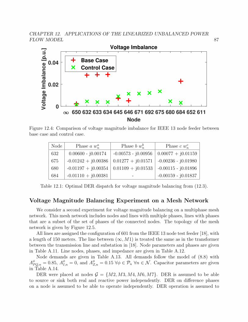
CHAPTER 12. APPLICATIONS OF THE LINEARIZED UNBALANCED POWERFLOW MODEL 87
650 632 633 634 645 646 671 692 675 680 684 652 611
Node
0
0.02
0.04
Vo
ltag
e Im
bala
nce [
p.u
.] Voltage Imbalance
Base Case
Control Case
Figure 12.4: Comparison of voltage magnitude imbalance for IEEE 13 node feeder betweenbase case and control case.
Node Phase a wan Phase b wbn Phase c wcn
632 0.00600 - j0.00174 -0.00573 - j0.00956 0.00077 + j0.01159
675 -0.01242 + j0.00386 0.01277 + j0.01571 -0.00236 - j0.01980
680 -0.01197 + j0.00354 0.01109 + j0.01533 -0.00115 - j0.01896
684 -0.01110 + j0.00381 - -0.00159 - j0.01837
Table 12.1: Optimal DER dispatch for voltage magnitude balancing from (12.3).
Voltage Magnitude Balancing Experiment on a Mesh Network
We consider a second experiment for voltage magnitude balancing on a multiphase meshnetwork. This mesh network includes nodes and lines with multiple phases, lines with phasesthat are a subset of the set of phases of the connected nodes. The topology of the meshnetwork is given by Figure 12.5.
All lines are assigned the configuration of 601 from the IEEE 13 node test feeder [18], witha length of 150 meters. The line between (∞,M1) is treated the same as in the transformerbetween the transmission line and substation in [18]. Node parameters and phases are givenin Table A.11. Line nodes, phases, and impedance are given in Table A.12.
Node demands are given in Table A.13. All demands follow the model of (8.8) withAφPQ,n = 0.85, AφI,n = 0, and AφZ,n = 0.15 ∀φ ∈ Pn ∀n ∈ N . Capacitor parameters are givenin Table A.14.
DER were placed at nodes G = {M2,M3,M4,M6,M7}. DER is assumed to be ableto source or sink both real and reactive power independently. DER on difference phaseson a node is assumed to be able to operate independently. DER operation is assumed to
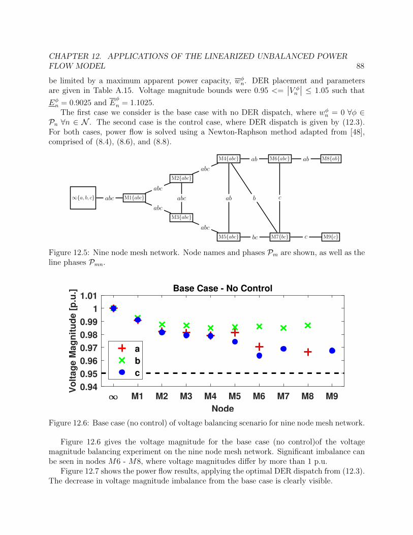
CHAPTER 12. APPLICATIONS OF THE LINEARIZED UNBALANCED POWERFLOW MODEL 88
be limited by a maximum apparent power capacity, wφn. DER placement and parametersare given in Table A.15. Voltage magnitude bounds were 0.95 <=
∣∣V φn
∣∣ ≤ 1.05 such that
Eφn = 0.9025 and E
φ
n = 1.1025.The first case we consider is the base case with no DER dispatch, where wφn = 0 ∀φ ∈
Pn ∀n ∈ N . The second case is the control case, where DER dispatch is given by (12.3).For both cases, power flow is solved using a Newton-Raphson method adapted from [48],comprised of (8.4), (8.6), and (8.8).
∞{a, b, c} M1{abc}abc
M2{abc}
abc
M3{abc}abc
abc
M4{abc}
abc
M5{abc}abc
ab
M6{abc}ab
M7{bc}bc
b c
M8{ab}ab
M9{c}c
Figure 12.5: Nine node mesh network. Node names and phases Pm are shown, as well as theline phases Pmn.
M1 M2 M3 M4 M5 M6 M7 M8 M9
Node
0.94
0.95
0.96
0.97
0.98
0.99
1
1.01
Vo
ltag
e M
ag
nit
ud
e [
p.u
.] Base Case - No Control
a
b
c
Figure 12.6: Base case (no control) of voltage balancing scenario for nine node mesh network.
Figure 12.6 gives the voltage magnitude for the base case (no control)of the voltagemagnitude balancing experiment on the nine node mesh network. Significant imbalance canbe seen in nodes M6 - M8, where voltage magnitudes differ by more than 1 p.u.
Figure 12.7 shows the power flow results, applying the optimal DER dispatch from (12.3).The decrease in voltage magnitude imbalance from the base case is clearly visible.
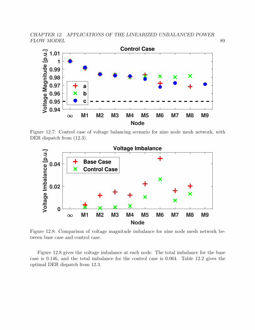
CHAPTER 12. APPLICATIONS OF THE LINEARIZED UNBALANCED POWERFLOW MODEL 89
M1 M2 M3 M4 M5 M6 M7 M8 M9
Node
0.94
0.95
0.96
0.97
0.98
0.99
1
1.01
Vo
ltag
e M
ag
nit
ud
e [
p.u
.] Control Case
a
b
c
Figure 12.7: Control case of voltage balancing scenario for nine node mesh network, withDER dispatch from (12.3).
M1 M2 M3 M4 M5 M6 M7 M8 M9
Node
0
0.02
0.04
Vo
ltag
e Im
bala
nce [
p.u
.] Voltage Imbalance
Base Case
Control Case
Figure 12.8: Comparison of voltage magnitude imbalance for nine node mesh network be-tween base case and control case.
Figure 12.8 gives the voltage imbalance at each node. The total imbalance for the basecase is 0.146, and the total imbalance for the control case is 0.064. Table 12.2 gives theoptimal DER dispatch from 12.3.
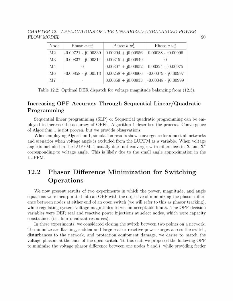
CHAPTER 12. APPLICATIONS OF THE LINEARIZED UNBALANCED POWERFLOW MODEL 90
Node Phase a wan Phase b wbn Phase c wcn
M2 -0.00721 - j0.00339 0.00294 + j0.00956 0.00088 - j0.00996
M3 -0.00837 - j0.00314 0.00315 + j0.00949 0
M4 0 0.00307 + j0.00952 0.00224 - j0.00975
M6 -0.00858 - j0.00513 0.00258 + j0.00966 -0.00079 - j0.00997
M7 - 0.00359 + j0.00933 -0.00048 - j0.00999
Table 12.2: Optimal DER dispatch for voltage magnitude balancing from (12.3).
Increasing OPF Accuracy Through Sequential Linear/QuadraticProgramming
Sequential linear programming (SLP) or Sequential quadratic programming can be em-ployed to increase the accuracy of OPFs. Algorithm 1 describes the process. Convergenceof Algorithm 1 is not proven, but we provide observations.
When employing Algorithm 1, simulation results show convergence for almost all networksand scenarios when voltage angle is excluded from the LUPFM as a variable. When voltageangle is included in the LUPFM, 1 usually does not converge, with differences in X and X∗
corresponding to voltage angle. This is likely due to the small angle approximation in theLUPFM.
12.2 Phasor Difference Minimization for Switching
Operations
We now present results of two experiments in which the power, magnitude, and angleequations were incorporated into an OPF with the objective of minimizing the phasor differ-ence between nodes at either end of an open switch (we will refer to this as phasor tracking),while regulating system voltage magnitudes to within acceptable limits. The OPF decisionvariables were DER real and reactive power injections at select nodes, which were capacityconstrained (i.e. four-quadrant resources).
In these experiments, we considered closing the switch between two points on a network.To minimize arc flashing, sudden and large real or reactive power surges across the switch,disturbances to the network, and protection equipment damage, we desire to match thevoltage phasors at the ends of the open switch. To this end, we proposed the following OPFto minimize the voltage phasor difference between one nodes k and l, while providing feeder
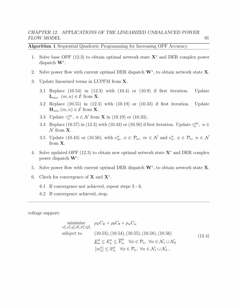
CHAPTER 12. APPLICATIONS OF THE LINEARIZED UNBALANCED POWERFLOW MODEL 91
Algorithm 1 Sequential Quadratic Programming for Increasing OPF Accuracy
1. Solve base OPF (12.3) to obtain optimal network state X∗ and DER complex powerdispatch W∗.
2. Solve power flow with current optimal DER dispatch W∗, to obtain network state X.
3. Update linearized terms in LUPFM from X.
3.1 Replace (10.54) in (12.3) with (10.4) or (10.9) if first iteration. UpdateLmn, (m,n) ∈ E from X.
3.2 Replace (10.55) in (12.3) with (10.19) or (10.33) if first iteration. UpdateHmn, (m,n) ∈ E from X.
3.3 Update γφψn , n ∈ N from X in (10.19) or (10.33).
3.4 Replace (10.57) in (12.3) with (10.43) or (10.50) if first iteration. Update γφψn , n ∈N from X.
3.5 Update (10.43) or (10.50), with eφm, φ ∈ Pm, m ∈ N and eφn, φ ∈ Pn, n ∈ Nfrom X.
4. Solve updated OPF (12.3) to obtain new optimal network state X∗ and DER complexpower dispatch W∗.
5. Solve power flow with current optimal DER dispatch W∗, to obtain network state X.
6. Check for convergence of X and X∗.
6.1 If convergence not achieved, repeat steps 3 - 6.
6.2 If convergence achieved, stop.
voltage support:
minimizeuφn,v
φn,y
φn,θ
φn,P
φn ,Q
φn
ρECE + ρθCθ + ρwCw
subject to (10.53), (10.54), (10.55), (10.58), (10.56)
Eφn ≤ Eφ
n ≤ Eφ
n ∀φ ∈ Pn, ∀n ∈ N1 ∪N2∣∣wφn∣∣ ≤ wφn ∀φ ∈ Pn, ∀n ∈ N1 ∪N2 ,
(12.4)
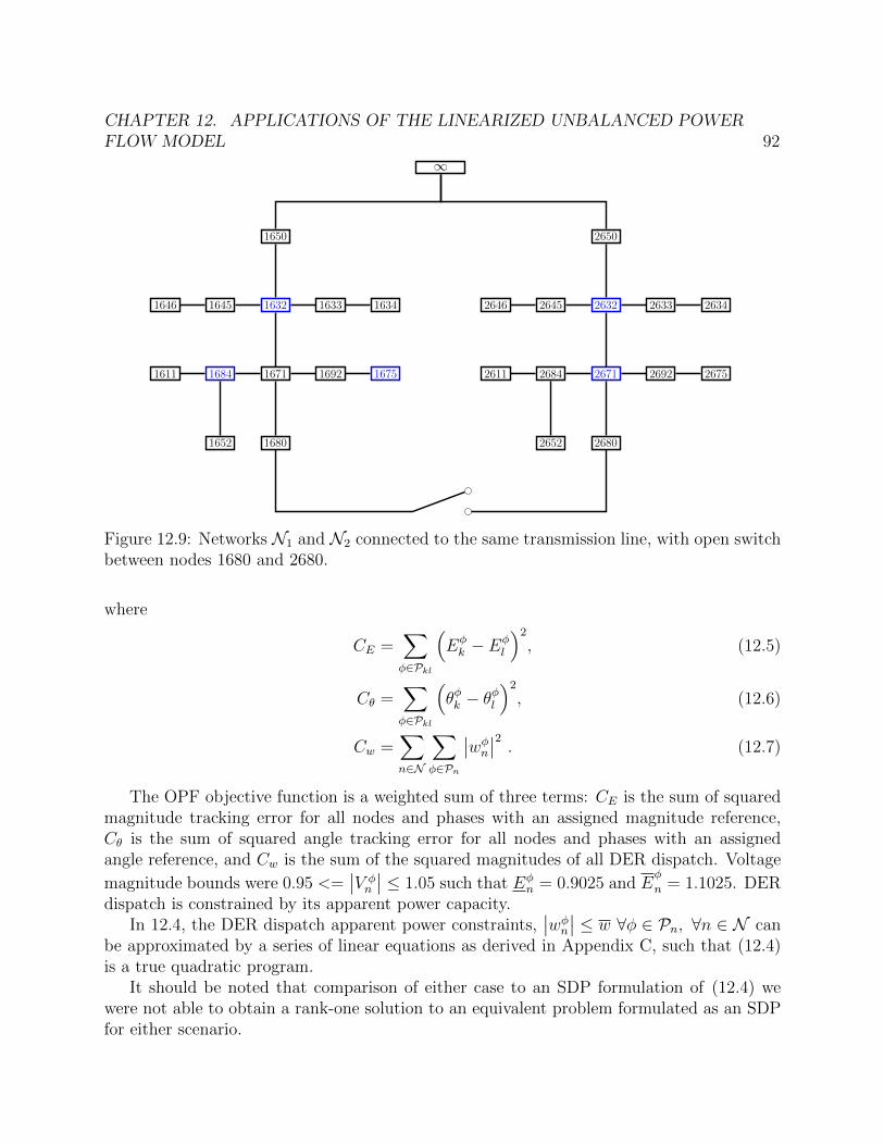
CHAPTER 12. APPLICATIONS OF THE LINEARIZED UNBALANCED POWERFLOW MODEL 92
∞
1650
1632 1633 163416451646
1671 1692 1675
1680
1684
1652
1611
2650
2632 2633 263426452646
2671 2692 2675
2680
2684
2652
2611
Figure 12.9: Networks N1 and N2 connected to the same transmission line, with open switchbetween nodes 1680 and 2680.
where
CE =∑φ∈Pkl
(Eφk − E
φl
)2, (12.5)
Cθ =∑φ∈Pkl
(θφk − θ
φl
)2, (12.6)
Cw =∑n∈N
∑φ∈Pn
∣∣wφn∣∣2 . (12.7)
The OPF objective function is a weighted sum of three terms: CE is the sum of squaredmagnitude tracking error for all nodes and phases with an assigned magnitude reference,Cθ is the sum of squared angle tracking error for all nodes and phases with an assignedangle reference, and Cw is the sum of the squared magnitudes of all DER dispatch. Voltage
magnitude bounds were 0.95 <=∣∣V φn
∣∣ ≤ 1.05 such that Eφn = 0.9025 and E
φ
n = 1.1025. DERdispatch is constrained by its apparent power capacity.
In 12.4, the DER dispatch apparent power constraints,∣∣wφn∣∣ ≤ w ∀φ ∈ Pn, ∀n ∈ N can
be approximated by a series of linear equations as derived in Appendix C, such that (12.4)is a true quadratic program.
It should be noted that comparison of either case to an SDP formulation of (12.4) wewere not able to obtain a rank-one solution to an equivalent problem formulated as an SDPfor either scenario.
CHAPTER 12. APPLICATIONS OF THE LINEARIZED UNBALANCED POWERFLOW MODEL 93
Phasor Difference Minimization on a Radial Network
The first experiment was conducted on two modified versions of the IEEE 13 node dis-tribution test feeder model [18]. Feeder topology, line configuration, line impedance, linelength, and spot loads are specified in [18] and outlined in Appendix A.2. We consider twonetworks, N1 and N2, connected to the same transmission line as in Figure 12.9. For clarity,we concatenate the number 1 to the front of nodes within N1 and the number 2 for nodeswithin N2 (e.g. node 671 of N1 is now 1671 and node 634 of N2 is now 2634). The trans-mission line, indexed by ∞ and denoted in Figure 12.9 by ∞, is treated as an infinite bus,
with fixed voltage reference of V∞ =[1 1∠240◦ 1∠120◦
]Tp.u..
The first network, N1, is a modified version of the IEEE 13 node test feeder model.The voltage regulator between nodes 1650 and 1632 is omitted, the transformer betweennodes 1633 and 1634 is replaced by a line of configuration 601 and length of 50 feet, andthe switch between node 1671 and 1692 is replaced by a line with configuration 601 andlength of 50 feet. All loads are assumed to be Wye connected. We place Wye connected0.01 + j0.004 p.u. loads on all phases at node 1680. Capacitors in N1 were multiplied bya factor of 0.5. Four quadrant capable DER were placed at on all existing phases at nodesG∞ = {1632, 1675, 1684}. We assumed each DER can inject or sink both real and reactivepower separately on each phase of the feeder. All DER were constrained by an apparentpower capacity limit on each phase of 250 kVA, or 0.05 p.u.
The second network, N2, is also a modified version of the IEEE 13 node test feedermodel. The voltage regulator between nodes 2650 and 2632 is omitted, the transformerbetween nodes 2633 and 2634 is replaced by a line of configuration 601 and length of 50 feet,and the switch between node 2671 and 2692 is replaced by a line with configuration 601 andlength of 50 feet. All loads are assumed to be Wye connected. We place Wye connected0.01 + j0.004 p.u. loads on all phases at node 2680. Capacitors in N1 were multiplied bya factor of 0.5. Four quadrant capable DER were placed at on all existing phases at nodesG∞ = {2632, 2671}. We assumed each DER can inject or sink both real and reactive powerseparately on each phase of the feeder. All DER were constrained by an apparent powercapacity limit on each phase of 250 kVA, or 0.05 p.u.
Loads follow the voltage dependent load model of (8.8) with parameters AφPQ,n = 0.85
and AφZ,n = 0.15 ∀φ ∈ {a, b, c}, ∀n ∈ N1, ∀n ∈ N2. To create a load imbalance between thetwo networks, we multiply all loads in N1 by a factor of 0.75 and all loads in N2 by a factorof 1.5. An open switch was placed between node k = 1680 of N1 and node l = 2680 of N2,with a line with configuration 601 and length of 500 feet.
The weighting on the three components of the objective function of (12.4) are ρE = 1000,ρθ = 1000, and ρw = 1. Results from this experiment can be seen in Table 12.3. Weconsider three cases: “No Control” (NC) where all DER dispatch is 0, “Magnitude Control”(MC) where the optimal DER dispatch is obtained solving (12.4) with ρθ = 0, and “PhasorControl” (PC) where the optimal DER dispatch is obtained solving (12.4). For each case,power flow is solved with the zero (NC) or optimal DER dispatch from (12.4) (MC,PC). For
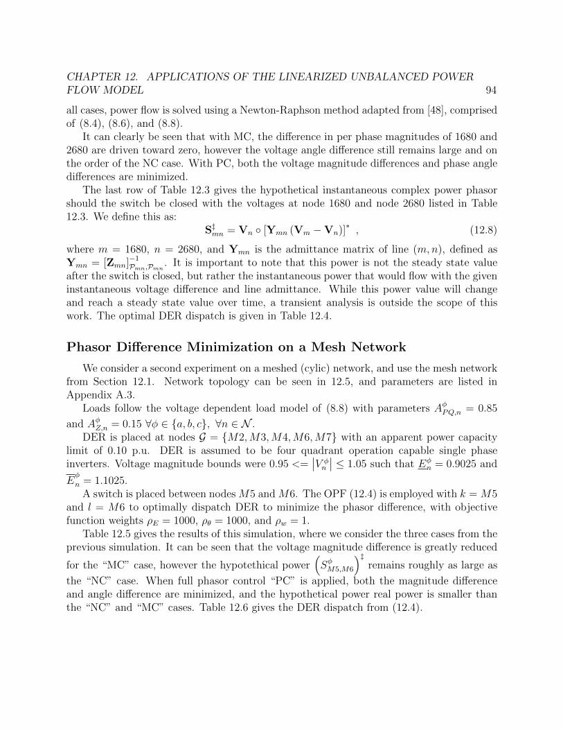
CHAPTER 12. APPLICATIONS OF THE LINEARIZED UNBALANCED POWERFLOW MODEL 94
all cases, power flow is solved using a Newton-Raphson method adapted from [48], comprisedof (8.4), (8.6), and (8.8).
It can clearly be seen that with MC, the difference in per phase magnitudes of 1680 and2680 are driven toward zero, however the voltage angle difference still remains large and onthe order of the NC case. With PC, both the voltage magnitude differences and phase angledifferences are minimized.
The last row of Table 12.3 gives the hypothetical instantaneous complex power phasorshould the switch be closed with the voltages at node 1680 and node 2680 listed in Table12.3. We define this as:
S‡mn = Vn ◦ [Ymn (Vm −Vn)]∗ , (12.8)
where m = 1680, n = 2680, and Ymn is the admittance matrix of line (m,n), defined asYmn = [Zmn]−1Pmn,Pmn . It is important to note that this power is not the steady state valueafter the switch is closed, but rather the instantaneous power that would flow with the giveninstantaneous voltage difference and line admittance. While this power value will changeand reach a steady state value over time, a transient analysis is outside the scope of thiswork. The optimal DER dispatch is given in Table 12.4.
Phasor Difference Minimization on a Mesh Network
We consider a second experiment on a meshed (cylic) network, and use the mesh networkfrom Section 12.1. Network topology can be seen in 12.5, and parameters are listed inAppendix A.3.
Loads follow the voltage dependent load model of (8.8) with parameters AφPQ,n = 0.85
and AφZ,n = 0.15 ∀φ ∈ {a, b, c}, ∀n ∈ N .DER is placed at nodes G = {M2,M3,M4,M6,M7} with an apparent power capacity
limit of 0.10 p.u. DER is assumed to be four quadrant operation capable single phaseinverters. Voltage magnitude bounds were 0.95 <=
∣∣V φn
∣∣ ≤ 1.05 such that Eφn = 0.9025 and
Eφ
n = 1.1025.A switch is placed between nodes M5 and M6. The OPF (12.4) is employed with k = M5
and l = M6 to optimally dispatch DER to minimize the phasor difference, with objectivefunction weights ρE = 1000, ρθ = 1000, and ρw = 1.
Table 12.5 gives the results of this simulation, where we consider the three cases from theprevious simulation. It can be seen that the voltage magnitude difference is greatly reduced
for the “MC” case, however the hypotethical power(SφM5,M6
)‡remains roughly as large as
the “NC” case. When full phasor control “PC” is applied, both the magnitude differenceand angle difference are minimized, and the hypothetical power real power is smaller thanthe “NC” and “MC” cases. Table 12.6 gives the DER dispatch from (12.4).
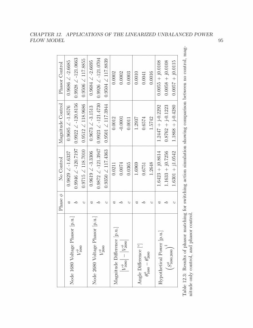
CHAPTER 12. APPLICATIONS OF THE LINEARIZED UNBALANCED POWERFLOW MODEL 95
Phas
eφ
No
Con
trol
Mag
nit
ude
Con
trol
Phas
orC
ontr
ol
Node
1680
Vol
tage
Phas
or[p
.u.]
Vφ 1680
a0.
9829
∠-1
.633
70.
9685
∠-1
.857
60.
9686
∠-2
.668
5
b0.
9946
∠-1
20.7
197
0.99
22∠
-120
.815
60.
9928
∠-1
21.0
663
c0.
9715
∠11
8.70
100.
9512
∠11
8.96
860.
9506
∠11
7.88
55
Node
2680
Vol
tage
Phas
or[p
.u.]
Vφ 2680
a0.
9619
∠-3
.330
60.
9673
∠-3
.151
30.
9684
∠-2
.669
5
b0.
9872
∠-1
21.3
947
0.99
23∠
-121
.473
00.
9926
∠-1
21.0
704
c0.
9350
∠11
7.43
630.
9501
∠11
7.39
440.
9504
∠11
7.88
39
Mag
nit
ude
Diff
eren
ce[p
.u.]
∣ ∣ ∣Vφ 1680
∣ ∣ ∣−∣ ∣ ∣Vφ 2680
∣ ∣ ∣a
0.02
110.
0012
0.00
02
b0.
0074
-0.0
001
0.00
02
c0.
0365
0.00
110.
0003
Angl
eD
iffer
ence
[◦]
θφ 1680−θφ 2
680
a1.
6969
1.29
370.
0010
b0.
6751
0.65
740.
0041
c1.
2648
1.57
420.
0016
Hyp
othet
ical
Pow
er[p
.u.]
( Sφ 1680,2680
) ‡a
1.64
23+
j0.8
614
1.24
47+
j-0.
2292
0.00
55+
j0.0
108
b1.
1633
+j0
.725
60.
8762
+j-
0.12
230.
0058
+j0
.010
8
c1.
6301
+j1
.054
21.
1868
+j-
0.42
800.
0057
+j0
.011
5
Tab
le12
.3:
Res
ult
sof
phas
orm
atch
ing
for
swit
chin
gac
tion
sim
ula
tion
show
ing
com
par
ison
bet
wee
nno
contr
ol,
mag
-nit
ude
only
contr
ol,
and
phas
orco
ntr
ol.
CHAPTER 12. APPLICATIONS OF THE LINEARIZED UNBALANCED POWERFLOW MODEL 96
Node Phase A Phase B Phase C
1632 0.0312 + j0.0189 0.0329 + j0.0197 0.0383 + j0.0214
1675 0.0433 + j0.0251 0.0436 + j0.0244 0.0440 + j0.0238
1684 0.0431 + j0.0253 0 0.0441 + j0.0236
2632 -0.0349 + j-0.0139 -0.0273 + j-0.0188 -0.0378 + j-0.0328
2671 -0.0472 + j-0.0166 -0.0419 + j-0.0273 -0.0381 + j-0.0324
Table 12.4: Optimal DER dispatch for phasor matching for switching action from (12.4).

CHAPTER 12. APPLICATIONS OF THE LINEARIZED UNBALANCED POWERFLOW MODEL 97
Phas
eφ
No
Con
trol
Mag
nit
ude
Con
trol
Phas
orC
ontr
ol
Node
M5
Vol
tage
Phas
or[p
.u.]
Vφ 1680
a0.
9814
∠-0
.999
30.
9838
∠-0
.794
60.
9816
∠-1
.685
6
b0.
9855
∠-1
20.9
524
0.98
04∠
-120
.827
30.
9968
∠-1
20.4
100
c0.
9744
∠11
8.43
290.
9902
∠11
8.42
580.
9629
∠11
9.27
20
Node
M6
Vol
tage
Phas
or[p
.u.]
Vφ 2680
a0.
9705
∠-1
.219
70.
9792
∠-1
.102
70.
9762
∠-1
.725
6
b0.
9860
∠-1
21.3
005
0.97
95∠
-120
.835
60.
9941
∠-1
20.4
713
c0.
9636
∠11
7.78
750.
9882
∠11
7.86
040.
9517
∠11
9.15
03
Mag
nit
ude
Diff
eren
ce[p
.u.]
∣ ∣ ∣Vφ M5
∣ ∣ ∣−∣ ∣ ∣Vφ M6
∣ ∣ ∣a
0.01
100.
0046
0.00
54
b-0
.000
50.
0009
0.00
27
c0.
0107
0.00
210.
0112
Angl
eD
iffer
ence
[◦]
θφ M5−θφ M
6
a0.
2205
0.30
810.
0400
b0.
3481
0.00
830.
0613
c0.
6454
0.56
540.
1217
Hyp
othet
ical
Pow
er[p
.u.]
( Sφ M
5,M
6
) ‡a
0.34
81+
j0.5
246
0.39
51+
j0.2
329
0.08
67+
j0.3
426
b0.
3137
+j0
.031
10.
0925
+j0
.076
90.
1405
+j0
.206
2
c0.
7499
+j0
.325
10.
4886
+j-
0.07
970.
2669
+j0
.449
5
Tab
le12
.5:
Res
ult
sof
phas
orm
atch
ing
for
swit
chin
gac
tion
sim
ula
tion
show
ing
com
par
ison
bet
wee
nno
contr
ol,
mag
-nit
ude
only
contr
ol,
and
phas
orco
ntr
ol.
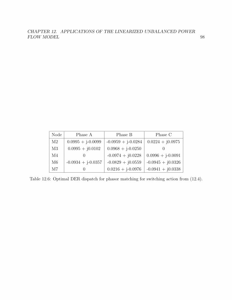
CHAPTER 12. APPLICATIONS OF THE LINEARIZED UNBALANCED POWERFLOW MODEL 98
Node Phase A Phase B Phase C
M2 0.0995 + j-0.0099 -0.0959 + j-0.0284 0.0224 + j0.0975
M3 0.0995 + j0.0102 0.0968 + j-0.0250 0
M4 0 -0.0974 + j0.0228 0.0996 + j-0.0091
M6 -0.0934 + j-0.0357 -0.0829 + j0.0559 -0.0945 + j0.0326
M7 0 0.0216 + j-0.0976 -0.0941 + j0.0338
Table 12.6: Optimal DER dispatch for phasor matching for switching action from (12.4).
99
Chapter 13
Concluding Remarks and FutureWork
Optimization of energy resources on unbalanced networks is a challenging field due to thenonlinear and nonconvex physics of power flow. Many works have studied how to addressthese issues using semidefinite programming and approximate linear models.
In this work, we our aim was to investigate solving OPF problems that cannot be ad-dressed with SDP techniques. We extend the work of [14, 20, 39] by developing a linearizedmodel for unbalanced power flow in Section 10.4. This model maps voltage angle differencesacross a line to the complex power flow on the line.
In Chapter 11, We investigated the accuracy of the LUPFM, comparing the results ofsolving power flow with the system physics and the LUPFM. We found that under normaloperating conditions, the model leads to magnitude errors on the order of 1%, angle errorsof less than 0.5 and substation power errors of 5% of the network rated power.
In Chapter 12, we study two applications of the LUPFM. The first application is tominimize the difference in voltage magnitude across different phases at nodes in a distributionnetwork. Simulation results prove the OPF effective in this endeavor.
The second application is to minimize the voltage phasor difference between two nodes,representing an open switch. We design an OPF that seeks to minimize the voltage mag-nitude difference per phase at two nodes, and the voltage angle difference per phase at twonodes. Simulation results demonstrate the efficacy of the OPF in minimizing voltage phasordifference.
The ability to switch components into and out of distribution feeders with minimal impacton system operation presents many opportunities to reconfigure distribution systems for avariety of purposes. Moving forward, we intend to investigate two such applications. First,we plan to study grid reconfiguration in order to better withstand critical grid events (e.g.weather-related or other types of disasters). In anticipation of a critical event, it may beadvantageous to alter system topology to maximize the ability to serve critical loads. Tosolve such a problem, we will most likely need to extend our present OPF formulation intoa receding horizon controller, that can optimize over a future time window. Secondly, as

CHAPTER 13. CONCLUDING REMARKS AND FUTURE WORK 100
“clean” switching may also enable distributed microgrids to coalesce and pool resources toprovide ancillary services, we intend to extend this OPF formulation to allow for mixed-integer formulations.
101
Chapter 14
Conclusion
14.1 Modeling and Optimal Control of Commercial
Office Plug Loads and Battery Storage Systems
This dissertation developed an approach for control of commercial office OSBS alongsideplug loads.
Summary of Results
This work focused on two main aspects: development of a model for an off the shelf OSBSfor incorporation into an MPC, and solving the nonlinear and nonconvex MPC. A modelpredictive control formulation was augmented to include generic battery storage for demandresponse of load following. A model of an off the shelf OSBS was derived from experimentaldata. Two algorithms for solving the nonlinear MPC were derived and discussed.
An exhaustive search algorithm that optimizes plug load control over all possible batterycontrol sequences was derived. Simulations with this algorithm highlight the severe faults ofshort prediction horizon and necessity of long timesteps.
A dynamic programming algorithm was then implemented. Simulation results show thepromise of this method, and highlight positive attributes such as long prediction windowand good timestep granularity. Simulation results also provide insight into the benefit of anOSBS with controllable charging.
Future Work
While the research in this work provided methods for control of plug loads and an OSBS,more work is needed before such work can be practically implemented. One key area is thedevelopment of an algorithm for optimal OSBS control for OSBS systems.
CHAPTER 14. CONCLUSION 102
14.2 Modeling of Unbalanced Power Flow and
Optimal Control of Distributed Energy
Resources for Grid Reconfiguration
This dissertation focused on approaches for controlling voltage magnitude and phaseangle on an unbalanced distribution network.
Summary of Results
First semidefinite programming is discussed as a method for solving nonlinear and non-convex OPFs. Literature points to many successes, but also bring to light many drawbacksand attributes of SDP that may preclude its widespread implementation. We then deriveseveral SDP OPFs for control of voltage magnitude and angle. Simulations motivate furtheranalysis into the control of voltage magnitude, and also show success in constraining voltageangle.
A linearized unbalanced power flow model (LUPFM) is derived for incorporation intoconvex OPFs. This model augments those of [14, 39] by adding a relationship betweenvoltage angle difference across a network line and complex power flow on the line. Theaccuracy of the LUPFM is investigated and found to be satisfactory for IEEE benchmarkunbalanced networks.
Two application of the LUPFM are discussed. The first is an OPF that seeks to minimizevoltage magnitude imbalance at nodes on an unbalanced network. Simulation results for bothradial and mesh networks show the success of this OPF.
The second is an OPF that seeks to minimize voltage phasor difference between twounconnected nodes for switching actions. Simulations for both radial and mesh networks aresuccessful in reducing the phasor difference.
Future Work
There are many key areas in which the LUPFM can improve distribution network oper-ation. An example is to incorporate the LUPFM into an MPC for voltage phasor regulationacross changing loads and distributed generation and storage conditions.
There are also many ways in which the LUPFM can be improved itself. Development ofmore accurate inverter models is a necessary task. Development of additional operationalnetwork constraints for the LUPFM is also necessary. Finally, a more thorough investigationinto sequential linear programming would likely prove beneficial.

103
Bibliography
[1] D. B. Arnold et al. “Model-Free Optimal Coordination of Distributed Energy Resourcesfor Provisioning Transmission-Level Services”. In: IEEE Transactions on Power Sys-tems PP.99 (2017), pp. 1–1. issn: 0885-8950. doi: 10.1109/TPWRS.2017.2707405.
[2] Daniel B Arnold, Michael D Sankur, and David M Auslander. “An energy informationgateway for use in residential and commercial environments”. In: Power and EnergySociety General Meeting (PES), 2012 IEEE. IEEE. 2012, pp. 1–5.
[3] Daniel B Arnold, Michael D Sankur, and David M Auslander. “Optimal Control ofOffice Plug-loads for Commercial Building Demand Response”. In: ASME 2013 Dy-namic Systems and Control Conference. American Society of Mechanical Engineers.2013, V001T13A001–V001T13A001.
[4] Daniel B Arnold, Michael D Sankur, and David M Auslander. “The next generationenergy information gateway for use in residential and commercial environments”. In:Power and Energy Society General Meeting (PES), 2013 IEEE. IEEE. 2013, pp. 1–5.
[5] Daniel B Arnold et al. “Model-Free Optimal Control of VAR Resources in DistributionSystems: An Extremum Seeking Approach”. In: IEEE Transactions on Power SystemsPP (99 2015), pp. 1–11.
[6] Daniel B Arnold et al. “Optimal dispatch of reactive power for voltage regulation andbalancing in unbalanced distribution systems”. In: IEEE Power and Energy SocietyGeneral Meeting, accepted (2016).
[7] Xiaoqing Bai et al. “Semidefinite programming for optimal power flow problems”. In:International Journal of Electrical Power & Energy Systems 30.6 (2008), pp. 383–392.
[8] Mesut E Baran and Felix F Wu. “Network reconfiguration in distribution systemsfor loss reduction and load balancing”. In: IEEE Transactions on Power delivery 4.2(1989), pp. 1401–1407.
[9] Mesut E Baran and Felix F Wu. “Optimal sizing of capacitors placed on a radialdistribution system”. In: IEEE Transactions on Power Delivery 4.1 (1989), pp. 735–743.
[10] Saverio Bolognani and Florian Dorfler. “Fast power system analysis via implicit lin-earization of the power flow manifold”. In: Communication, Control, and Computing(Allerton), 2015 53rd Annual Allerton Conference on. IEEE. 2015, pp. 402–409.
BIBLIOGRAPHY 104
[11] Emiliano Dall’Anese, Hao Zhu, and Georgios Giannakis. “Distributed optimal powerflow for smart microgrids”. In: Smart Grid, IEEE Transactions on 4.3 (2013), pp. 1464–1475.
[12] Masoud Farivar, Lijun Chen, and Steven Low. “Equilibrium and dynamics of localvoltage control in distribution systems”. In: Decision and Control (CDC), 2013 IEEE52nd Annual Conference on. IEEE. 2013, pp. 4329–4334.
[13] John Franco, Luis Ochoa, and Ruben Romero. “AC OPF for Smart Distribution Net-works: An Efficient and Robust Quadratic Approach”. In: IEEE Transactions on SmartGrid (2017).
[14] Lingwen Gan and Steven H Low. “Convex relaxations and linear approximation foroptimal power flow in multiphase radial networks”. In: Power Systems ComputationConference (PSCC), 2014. IEEE. 2014, pp. 1–9.
[15] Grid Modernization Multi-Year Program Plan. http://energy.gov/sites/prod/files / 2016 / 01 / f28 / Grid \ %20Modernization \ %20Multi - Year \ %20Program \
%20Plan.pdf.
[16] Gerald Thomas Heydt. “The next generation of power distribution systems”. In: IEEETransactions on Smart Grid 1.3 (2010), pp. 225–235.
[17] Longbo Huang, Jean Walrand, and Kannan Ramchandran. “Optimal demand re-sponse with energy storage management”. In: Smart Grid Communications (Smart-GridComm), 2012 IEEE Third International Conference on. IEEE. 2012, pp. 61–66.
[18] IEEE Distribution Test Feeders. http://ewh.ieee.org/soc/pes/dsacom/testfeeders/index.html. Online; accessed May-2015.
[19] David Kaneda et al. “Plug load reduction: The next big hurdle for net zero energy build-ing design”. In: published in the ACEEE Summer Study on Energy Efficient Buildings(2010), pp. 9–120.
[20] Vassilis Kekatos et al. “Voltage regulation algorithms for multiphase power distributiongrids”. In: IEEE Transactions on Power Systems 31.5 (2016), pp. 3913–3923.
[21] Iordanis Koutsopoulos, Vassiliki Hatzi, and Leandros Tassiulas. “Optimal energy stor-age control policies for the smart power grid”. In: Smart Grid Communications (Smart-GridComm), 2011 IEEE International Conference on. IEEE. 2011, pp. 475–480.
[22] Javad Lavaei and Steven H Low. “Zero duality gap in optimal power flow problem”.In: IEEE Transactions on Power Systems 27.1 (2012), pp. 92–107.
[23] Javad Lavaei, David Tse, and Baosen Zhang. “Geometry of power flows and optimiza-tion in distribution networks”. In: IEEE Transactions on Power Systems 29.2 (2014),pp. 572–583.
[24] Bernard C Lesieutre et al. “Examining the limits of the application of semidefiniteprogramming to power flow problems”. In: Communication, Control, and Computing(Allerton), 2011 49th Annual Allerton Conference on. IEEE. 2011, pp. 1492–1499.
BIBLIOGRAPHY 105
[25] Na Li, Guannan Qu, and Munther Dahleh. “Real-time decentralized voltage control indistribution networks”. In: Communication, Control, and Computing (Allerton), 201452nd Annual Allerton Conference on. IEEE. 2014, pp. 582–588.
[26] Raphael Louca, Peter Seiler, and Eilyan Bitar. “A rank minimization algorithm toenhance semidefinite relaxations of optimal power flow”. In: Communication, Control,and Computing (Allerton), 2013 51st Annual Allerton Conference on. IEEE. 2013,pp. 1010–1020.
[27] Raphael Louca, Peter Seiler, and Eilyan Bitar. “Nondegeneracy and inexactness ofsemidefinite relaxations of optimal power flow”. In: arXiv preprint arXiv:1411.4663(2014).
[28] Zhi-Quan Luo et al. “Semidefinite relaxation of quadratic optimization problems”. In:IEEE Signal Processing Magazine 27.3 (2010), pp. 20–34.
[29] Ramtin Madani, Somayeh Sojoudi, and Javad Lavaei. “Convex relaxation for optimalpower flow problem: Mesh networks”. In: IEEE Transactions on Power Systems 30.1(2015), pp. 199–211.
[30] A. von Meier et al. “Micro-synchrophasors for distribution systems”. In: ISGT 2014.Feb. 2014, pp. 1–5. doi: 10.1109/ISGT.2014.6816509.
[31] Daniel K Molzahn, Sina S Baghsorkhi, and Ian A Hiskens. “Semidefinite relaxationsof equivalent optimal power flow problems: An illustrative example”. In: Circuits andSystems (ISCAS), 2015 IEEE International Symposium on. IEEE. 2015, pp. 1887–1890.
[32] Daniel K Molzahn and Ian A Hiskens. “Convex relaxations of optimal power flowproblems: An illustrative example”. In: IEEE Transactions on Circuits and Systems I:Regular Papers 63.5 (2016), pp. 650–660.
[33] Daniel K Molzahn et al. “Implementation of a large-scale optimal power flow solverbased on semidefinite programming”. In: IEEE Transactions on Power Systems 28.4(2013), pp. 3987–3998.
[34] Nathan Murthy. “Energy-agile laptops: Demand response of mobile plug loads usingsensor/actuator networks”. In: Smart Grid Communications (SmartGridComm), 2012IEEE Third International Conference on. IEEE. 2012, pp. 581–586.
[35] Luis F Ochoa and Douglas H Wilson. “Angle constraint active management of distri-bution networks with wind power”. In: Innovative Smart Grid Technologies ConferenceEurope (ISGT Europe), 2010 IEEE PES. IEEE. 2010, pp. 1–5.
[36] Frauke Oldewurtel et al. “Reducing peak electricity demand in building climate controlusing real-time pricing and model predictive control”. In: Decision and Control (CDC),2010 49th IEEE Conference on. IEEE. 2010, pp. 1927–1932.
[37] Quadrennial Energy Review: First Installment. urlhttp://energy.gov/epsa/downloads/quadrennial-energy-review-first-installment. Online; April-2015.
BIBLIOGRAPHY 106
[38] He Renmu, Ma Jin, and David J Hill. “Composite load modeling via measurementapproach”. In: IEEE Transactions on Power Systems 21.2 (2006), pp. 663–672.
[39] Brett A Robbins and Alejandro D Domınguez-Garcıa. “Optimal reactive power dis-patch for voltage regulation in unbalanced distribution systems”. In: IEEE Transac-tions on Power Systems 31.4 (2016), pp. 2903–2913.
[40] Michael D Sankur, Daniel B Arnold, and David Auslander. “An architecture for inte-grated commercial building demand response”. In: Power and Energy Society GeneralMeeting (PES), 2013 IEEE. IEEE. 2013, pp. 1–5.
[41] Michael D Sankur, Daniel B Arnold, and David M Auslander. “Dynamic Programmingfor Optimal Load-Shedding of Office Scale Battery Storage and Plug-Loads”. In: Powerand Energy Society General Meeting (PES), 2015 IEEE. IEEE. 2015.
[42] Michael D Sankur, Daniel B Arnold, and David M Auslander. “Model Predictive Con-trol of Commercial Office Plug-Loads and Battery Storage Systems”. In: ASME 2014Dynamic Systems and Control Conference. American Society of Mechanical Engineers.2014, V001T07A001–V001T07A001.
[43] E M Stewart et al. Analysis of High-Penetration Levels of Photovoltaics into the Dis-tribution Grid on Oahu, Hawaii, Detailed Analysis of HECO Feeder WF1. Tech. rep.NREL subcontract report NREL/SR-5500-54494, 2013.
[44] Synchrophasor Fact Sheet. https://cdn.selinc.com/assets/Literature/Product\%20Literature / Flyers / FS _ Synchrophasor _ BF _ 20100617 . pdf ? v = 20150408 -
131001. Online; June-2010.
[45] Energy Information Administration (US). Annual Energy Review 2011. GovernmentPrinting Office, 2012.
[46] Peter Van de Ven et al. “Optimal control of residential energy storage under pricefluctuations”. In: ENERGY 2011, The First International Conference on Smart Grids,Green Communications and IT Energy-aware Technologies. 2011, pp. 159–162.
[47] Dongping Wang et al. “PMU-based angle constraint active management on 33kV distri-bution network”. In: Electricity Distribution (CIRED 2013), 22nd International Con-ference and Exhibition on. IET. 2013, pp. 1–4.
[48] RG Wasley and MA Shlash. “Newton-Raphson algorithm for 3-phase load flow”. In:Proceedings of the Institution of Electrical Engineers. Vol. 121. 7. IET. 1974, pp. 630–638.
[49] Thomas Weng et al. “Managing plug-loads for demand response within buildings”. In:Proceedings of the Third ACM Workshop on Embedded Sensing Systems for Energy-Efficiency in Buildings. ACM. 2011, pp. 13–18.
[50] Ahmed S Zamzam, Nicholas D Sidiropoulos, and Emiliano Dall’Anese. “Beyond re-laxation and Newton-Raphson: Solving AC OPF for multi-phase systems with renew-ables”. In: IEEE Transactions on Smart Grid (2016).

BIBLIOGRAPHY 107
[51] Baosen Zhang et al. “Optimal distributed voltage regulation in power distribution net-works”. In: Cornell University Library Web Page. Available online: http://arxiv.org/abs/1204.5226v1 (accessed on 23 April 2012) (2012).

108
Appendix A
Distribution Network Parameters
A.1 Parameters of the Five Node Network
This appendix will outline the parameters of the five node meshed network as used insimulations in Chapter 9. The topology can be seen in Figure 9.1.
Node ∞ A1 A2 A3 A4 A5
Pm {a} {a} {a} {a} {a} {a}
Table A.1: Five node network nodes parameters.
Node m Node n Pmn 100× [Zmn]Pmn [p.u.]
∞ A1 {a}[0.3281 + j0.9639
]A1 A2 {a}
[1.3125 + j3.8557
]A2 A3 {a}
[0.9844 + j2.8918
]A2 A4 {a}
[0.9844 + j2.8918
]A4 A5 {a}
[0.9844 + j2.8918
]Table A.2: Five node network line nodes, phases and impedances.

APPENDIX A. DISTRIBUTION NETWORK PARAMETERS 109
Node Phase a dan Phase b dbn Phase c dcn
A2 0.1000 + j0.0800 - -
A3 0.1000 + j0.1000 - -
A4 0.0600 + j0.0800 - -
A5 0.0600 + j0.0400 - -
Table A.3: Per-unit complex demands at nodes for nine node network
Node Phase a can Phase b cbn Phase c ccn
A5 j0.0400 - -
Table A.4: Per-unit capacitance at nodes for nine node network
Node Phase a wan Phase b wbn Phase c wcn
A2 0.1000 - -
A3 0.1000 - -
A5 0.1000 - -
Table A.5: Per-unit apparent power capacity for DER placed nine node network.
A.2 Parameters of the IEEE 13 Node Test Feeder
This appendix will outline the parameters of the IEEE 13 node test feeder as used insimulations in Chapter 11 and Chapter 12. The topology can be seen in Figure 11.1.
Node ∞ 650 632 633 634 645 646
Pm {a, b, c} {a, b, c} {a, b, c} {a, b, c} {a, b, c} {b, c} {b, c}Node 671 692 675 680 684 652 611
Pm {a, b, c} {a, b, c} {a, b, c} {a, b, c} {a, c} {a} {c}
Table A.6: IEEE 13 node test network nodes parameters from [18].
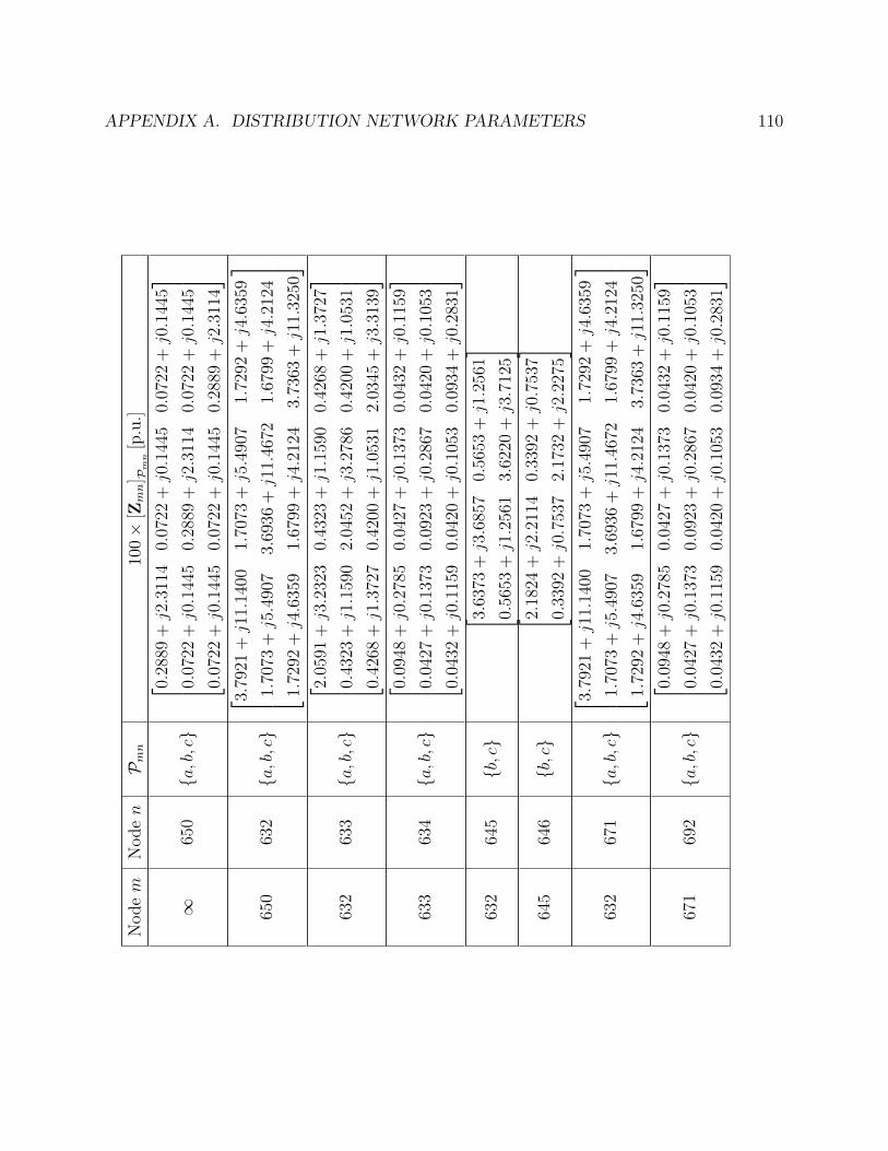
APPENDIX A. DISTRIBUTION NETWORK PARAMETERS 110N
odem
Noden
Pmn
100×
[Zmn] Pmn
[p.u
.]
∞65
0{a,b,c}
0.28
89+j2.3
114
0.07
22+j0.1
445
0.07
22+j0.1
445
0.07
22+j0.1
445
0.28
89+j2.3
114
0.07
22+j0.1
445
0.07
22+j0.1
445
0.07
22+j0.1
445
0.28
89+j2.3
114
650
632
{a,b,c}
3.79
21+j1
1.14
001.
7073
+j5.4
907
1.72
92+j4.6
359
1.70
73+j5.4
907
3.69
36+j1
1.46
721.
6799
+j4.2
124
1.72
92+j4.6
359
1.67
99+j4.2
124
3.73
63+j1
1.32
50
63
263
3{a,b,c}
2.05
91+j3.2
323
0.43
23+j1.1
590
0.42
68+j1.3
727
0.43
23+j1.1
590
2.04
52+j3.2
786
0.42
00+j1.0
531
0.42
68+j1.3
727
0.42
00+j1.0
531
2.03
45+j3.3
139
633
634
{a,b,c}
0.09
48+j0.2
785
0.04
27+j0.1
373
0.04
32+j0.1
159
0.04
27+j0.1
373
0.09
23+j0.2
867
0.04
20+j0.1
053
0.04
32+j0.1
159
0.04
20+j0.1
053
0.09
34+j0.2
831
632
645
{b,c}
[ 3.63
73+j3.6
857
0.56
53+j1.2
561
0.56
53+j1.2
561
3.62
20+j3.7
125]
645
646
{b,c}
[ 2.18
24+j2.2
114
0.33
92+j0.7
537
0.33
92+j0.7
537
2.17
32+j2.2
275]
632
671
{a,b,c}
3.79
21+j1
1.14
001.
7073
+j5.4
907
1.72
92+j4.6
359
1.70
73+j5.4
907
3.69
36+j1
1.46
721.
6799
+j4.2
124
1.72
92+j4.6
359
1.67
99+j4.2
124
3.73
63+j1
1.32
50
67
169
2{a,b,c}
0.09
48+j0.2
785
0.04
27+j0.1
373
0.04
32+j0.1
159
0.04
27+j0.1
373
0.09
23+j0.2
867
0.04
20+j0.1
053
0.04
32+j0.1
159
0.04
20+j0.1
053
0.09
34+j0.2
831
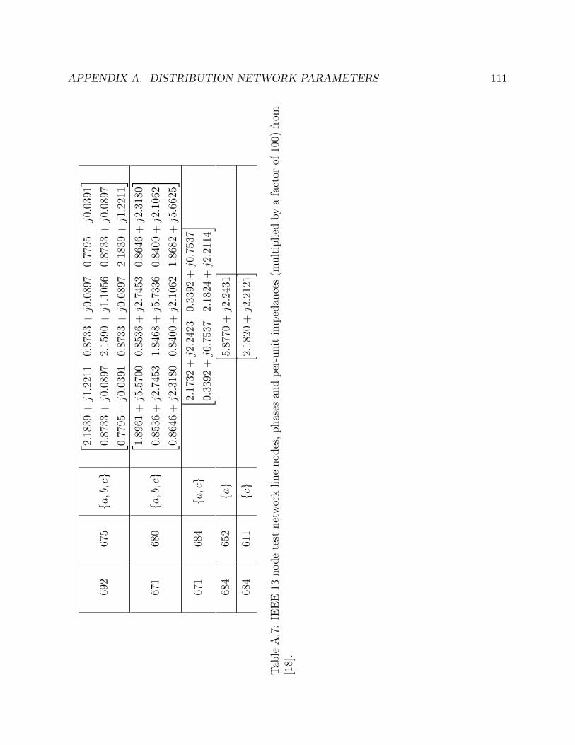
APPENDIX A. DISTRIBUTION NETWORK PARAMETERS 111
692
675
{a,b,c}
2.18
39+j1.2
211
0.87
33+j0.0
897
0.77
95−j0.0
391
0.87
33+j0.0
897
2.15
90+j1.1
056
0.87
33+j0.0
897
0.77
95−j0.0
391
0.87
33+j0.0
897
2.18
39+j1.2
211
671
680
{a,b,c}
1.89
61+j5.5
700
0.85
36+j2.7
453
0.86
46+j2.3
180
0.85
36+j2.7
453
1.84
68+j5.7
336
0.84
00+j2.1
062
0.86
46+j2.3
180
0.84
00+j2.1
062
1.86
82+j5.6
625
671
684
{a,c}
[ 2.17
32+j2.2
423
0.33
92+j0.7
537
0.33
92+j0.7
537
2.18
24+j2.2
114]
684
652
{a}
[ 5.87
70+j2.2
431]
684
611
{c}
[ 2.18
20+j2.2
121]
Tab
leA
.7:
IEE
E13
node
test
net
wor
kline
nodes
,phas
esan
dp
er-u
nit
imp
edan
ces
(mult
iplied
by
afa
ctor
of10
0)fr
om[1
8].

APPENDIX A. DISTRIBUTION NETWORK PARAMETERS 112
Node Phase a dan Phase b dbn Phase c dcn
634 0.0320 + j0.0220 0.0240 + j0.0180 0.0240 + j0.0180
645 - 0.0340 + j0.0250 0
646 - 0.0460 + j0.0264 0
671 0.0770 + j0.0440 0.0770 + j0.0440 0.0770 + j0.0440
692 0 0 0.0340 + j0.0302
675 0.0970 + j0.0380 0.0136 + j0.0120 0.0580 + j0.0424
680 0.0020 + j0.0010 0.0020 + j0.0010 0.0020 + j0.0010
652 0.0256 + j0.0172 - -
611 - - 0.0340 + j0.0160
Table A.8: Per-unit complex demands at nodes for IEEE 13 node feeder model from [18].
Node Phase a can Phase b cbn Phase c ccn
675 j0.0400 j0.0400 j0.0400
611 - - j0.0200
Table A.9: Per-unit capacitance at nodes for IEEE 13 node feeder from [18].
Node Phase a wan Phase b wbn Phase c wcn
632 0.0250 0.0250 0.0250
675 0.0250 0.0250 0.0250
680 0.0250 0.0250 0.0250
684 0.0250 - 0.0250
Table A.10: Per-unit apparent power capacity for DER placed on IEEE 13 node feeder.
A.3 Parameters of the Nine Node Meshed Network
This appendix will outline the parameters of the nine node meshed network as used insimulations in Chapter 12. The topology can be seen in Figure 12.5.

APPENDIX A. DISTRIBUTION NETWORK PARAMETERS 113
Node ∞ M1 M2 M3 M4
Pm {a, b, c} {a, b, c} {a, b, c} {a, b, c} {a, b, c}Node M5 M6 M7 M8 M9
Pm {a, b, c} {a, b, c} {b, c} {a, b} {c}
Table A.11: Nine node mesh network nodes parameters.

APPENDIX A. DISTRIBUTION NETWORK PARAMETERS 114N
odem
Noden
Pmn
100×
[Zmn] Pmn
[p.u
.]
∞M
1{a,b,c}
0.28
89+j2.3
114
0.07
22+j0.1
445
0.07
22+j0.1
445
0.07
22+j0.1
445
0.28
89+j2.3
114
0.07
22+j0.1
445
0.07
22+j0.1
445
0.07
22+j0.1
445
0.28
89+j2.3
114
M1
M2
{a,b,c}
0.93
31+j2.7
411
0.42
01+j1.3
510
0.42
55+j1.1
407
0.42
01+j1.3
510
0.90
89+j2.8
217
0.41
34+j1.0
365
0.42
55+j1.1
407
0.41
34+j1.0
365
0.91
94+j2.7
867
M2
M3
{a,b,c}
0.93
31+j2.7
411
0.42
01+j1.3
510
0.42
55+j1.1
407
0.42
01+j1.3
510
0.90
89+j2.8
217
0.41
34+j1.0
365
0.42
55+j1.1
407
0.41
34+j1.0
365
0.91
94+j2.7
867
M2
M3
{a,b,c}
0.93
31+j2.7
411
0.42
01+j1.3
510
0.42
55+j1.1
407
0.42
01+j1.3
510
0.90
89+j2.8
217
0.41
34+j1.0
365
0.42
55+j1.1
407
0.41
34+j1.0
365
0.91
94+j2.7
867
M2
M4
{a,b,c}
0.93
31+j2.7
411
0.42
01+j1.3
510
0.42
55+j1.1
407
0.42
01+j1.3
510
0.90
89+j2.8
217
0.41
34+j1.0
365
0.42
55+j1.1
407
0.41
34+j1.0
365
0.91
94+j2.7
867
M3
M5
{a,b,c}
0.93
31+j2.7
411
0.42
01+j1.3
510
0.42
55+j1.1
407
0.42
01+j1.3
510
0.90
89+j2.8
217
0.41
34+j1.0
365
0.42
55+j1.1
407
0.41
34+j1.0
365
0.91
94+j2.7
867
M4
M5
{a,b}
[ 0.93
31+j2.7
411
0.42
01+j1.3
510
0.42
01+j1.3
510
0.90
89+j2.8
217]
M4
M6
{a,b}
[ 0.93
31+j2.7
411
0.42
01+j1.3
510
0.42
01+j1.3
510
0.90
89+j2.8
217]
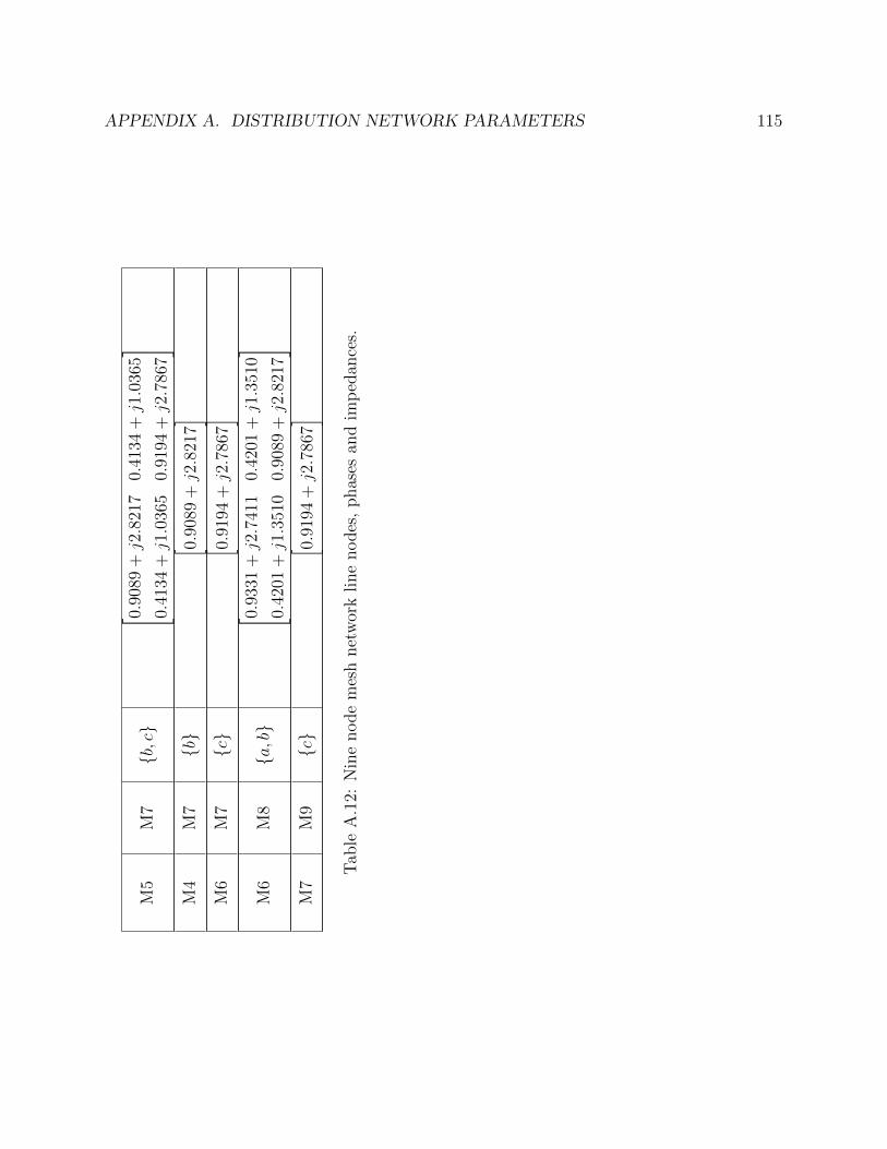
APPENDIX A. DISTRIBUTION NETWORK PARAMETERS 115
M5
M7
{b,c}
[ 0.90
89+j2.8
217
0.41
34+j1.0
365
0.41
34+j1.0
365
0.91
94+j2.7
867]
M4
M7
{b}
[ 0.90
89+j2.8
217]
M6
M7
{c}
[ 0.91
94+j2.7
867]
M6
M8
{a,b}
[ 0.93
31+j2.7
411
0.42
01+j1.3
510
0.42
01+j1.3
510
0.90
89+j2.8
217]
M7
M9
{c}
[ 0.91
94+j2.7
867]
Tab
leA
.12:
Nin
enode
mes
hnet
wor
kline
nodes
,phas
esan
dim
ped
ance
s.
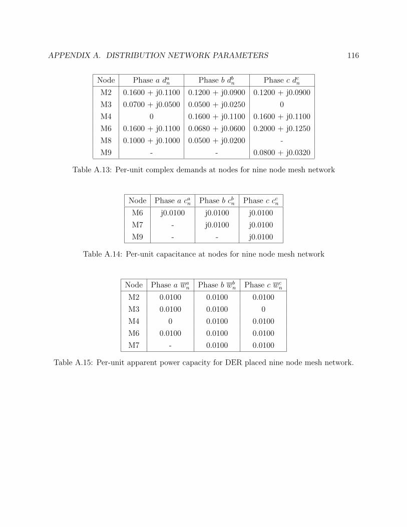
APPENDIX A. DISTRIBUTION NETWORK PARAMETERS 116
Node Phase a dan Phase b dbn Phase c dcn
M2 0.1600 + j0.1100 0.1200 + j0.0900 0.1200 + j0.0900
M3 0.0700 + j0.0500 0.0500 + j0.0250 0
M4 0 0.1600 + j0.1100 0.1600 + j0.1100
M6 0.1600 + j0.1100 0.0680 + j0.0600 0.2000 + j0.1250
M8 0.1000 + j0.1000 0.0500 + j0.0200 -
M9 - - 0.0800 + j0.0320
Table A.13: Per-unit complex demands at nodes for nine node mesh network
Node Phase a can Phase b cbn Phase c ccn
M6 j0.0100 j0.0100 j0.0100
M7 - j0.0100 j0.0100
M9 - - j0.0100
Table A.14: Per-unit capacitance at nodes for nine node mesh network
Node Phase a wan Phase b wbn Phase c wcn
M2 0.0100 0.0100 0.0100
M3 0.0100 0.0100 0
M4 0 0.0100 0.0100
M6 0.0100 0.0100 0.0100
M7 - 0.0100 0.0100
Table A.15: Per-unit apparent power capacity for DER placed nine node mesh network.

117
Appendix B
Newton-Raphson Algorithm forSolving Approximate UnbalancedPower Flow
This section presents the equations, residuals, and Jacobian terms for a Newton-Raphsonmethod that solves unbalanced approximate power flow. The method presented here incor-
porates A2, A3 where Hmn =[0 0 0
]T, A4 to both the magnitude and angle equations,
A5, and A6. Thus this method encompasses (10.53), (10.54), (10.55), (10.58), and (10.56).In this method, the pertinent variables are Eφ
n , θφn, P φmn, and Qφ
mn.
Line Real and Reactive Power
For a line (m,n) ∈ E , if φ /∈ Pmn then by definition:
P φmn = 0
Qφmn = 0 .
(B.1)
The residuals are defined as:∆P φ
mn = 0
∆Qφmn = 0 .
(B.2)
The partial derivative of the residuals are:
∂∆P φmn
∂P φmn
= 1
∂∆Qφmn
∂Qφmn
= 1 .
(B.3)

APPENDIX B. NEWTON-RAPHSON ALGORITHM FOR SOLVING APPROXIMATEUNBALANCED POWER FLOW 118
Magnitude Equation on Line (m,n)
For a line (m,n) ∈ E , if φ ∈ Pmn we consider (10.55) where Mmn, and Nmn, are definedby (10.58). For φ ∈ Pmn, the magnitude equation is:
Eφm = Eφ
n + 2∑
ψ∈Pmn
MφψmnP
ψmn −Nφψ
mnQψmn . (B.4)
The residual of the magnitude equation is:
∆Eφmn = −Eφ
m + Eφn + 2
∑ψ∈Pmn
MφψmnP
ψmn − 2Nφψ
mnQψmn . (B.5)
The partial derivatives of the magnitude equation residual are:
∂∆Eφmn
∂Eφm
= −1
∂∆Eφmn
∂Eφn
= 1
∂∆Eφmn
∂Pψmn
= 2Mφψmn ψ ∈ Pmn,
∂∆Eφmn
∂Qψmn
= −2Nφψmn ψ ∈ Pmn .
(B.6)
Angle equation on Line (m,n)
For a line (m,n) ∈ E , if φ ∈ Pmn we consider (10.56) where Mmn, and Nmn, are definedby (10.58), and eφm and eφn are fixed voltage magnitudes. For phase phi ∈ Pmn, the angleequation is:
eφmeφnθ
φm = eφme
φnθ
φn −
∑ψ∈Pmn
MφψmnP
ψmn +Nφψ
mnQψmn . (B.7)
The residuals of the magnitude equation is defined as:
∆θφmn = −eφmeφnθφm + eφmeφnθ
φn −
∑ψ∈Pmn
MφψmnP
ψmn +Nφψ
mnQψmn . (B.8)
The partial derivatives of the magnitude equation residuals are:
∂∆θφmn
∂θφm= −eφmeφn
∂∆θφmn
∂θφn= eφme
φn
∂∆θφmn
∂Pψmn
= −Nφψmn ψ ∈ Pmn
∂∆θφmn
∂Qψmn
= −Mφψmn ψ ∈ Pmn .
(B.9)

APPENDIX B. NEWTON-RAPHSON ALGORITHM FOR SOLVING APPROXIMATEUNBALANCED POWER FLOW 119
Node Voltage Magnitude and Angle
For a node n ∈ N , if φ /∈ Pn then the voltage magnitude and angle are:
Eφn = 0
θφn = 0 .(B.10)
The residuals of the voltage magnitude and angle are:
∆Eφn = Eφ
n
∆θφn = θφn .(B.11)
The partial derivative(s) of the residual of the voltage magnitude and angle are:
∂∆Eφn
∂Eφn
= 1
∂∆θφn
∂θφn= 1 .
(B.12)
Node Real Power Conservation
For a node m ∈ N , if φ ∈ Pn the conservation of real power, with pφm taken as the realcomponent of sφm, is:∑
l:(l,m)∈E
P φlm =
(AφPQ,m + AφZ,mE
φm
)Re{dφm}
+ uφm +∑
n:(m,n)∈E
P φmn . (B.13)
The residual of node real power conservation is:
∆pφm = −∑
l:(l,m)∈E
P φlm +
(AφPQ,m + AφZ,mE
φn
)Re{dφm}
+ uφm +∑
n:(m,n)∈E
P φmn . (B.14)
The partial derivatives of the residual of node real power conservation are:
∂∆pφm
∂P φlm
= −1
∂∆pφm
∂Eφm
= AφZ,m Re{dφm}
∂∆pφm
∂P φmn
= 1 .
(B.15)

APPENDIX B. NEWTON-RAPHSON ALGORITHM FOR SOLVING APPROXIMATEUNBALANCED POWER FLOW 120
Node Reactive Power Conservation
For a node m ∈ N , if φ ∈ Pn the conservation of reactive power, with qφm taken as theimaginary component of sφm, is:∑
l:(l,m)∈E
Qφlm =
(AφPQ,m + AφZ,mE
φm
)Im{dφm}
+ vφm − cφm +∑
n:(m,n)∈E
Qφmn . (B.16)
The residual of node real power conservation is:
∆qφm = −∑
l:(l,m)∈E
Qφlm +
(AφPQ,m + AφZ,mE
φn
)Im{dφm}
+ vφm − cφm +∑
n:(m,n)∈E
Pφmn . (B.17)
The partial derivatives of the residual of node real power conservation are:
∂∆qφm
∂Qφlm
= −1
∂∆qφm
∂Eφm
= AφZ,m Im{dφm}
∂∆qφm
∂Qφmn
= 1 .
(B.18)
Slack Node Voltage Magnitude and Angle
Solving power flow typically requires selecting a slack node and assigning a fixed voltagereference. The slack node voltage magnitude variable will be represented by Eφ
sl, and the
slack node voltage angle variable will be represented by θφsl. An overline notation will denotethe fixed voltage reference. At the slack node, the voltage magnitude and angle are:
Eφsl = Eφ
θφsl = θφ .(B.19)
The residuals of the slack bus voltage equations are:
∆Eφsl = Eφ
sl − Eφ
∆θφsl = θφsl − θφ .(B.20)
The partial derivatives of the residuals of the slack bus voltage equations are:
∂∆Eφsl
∂Eφsl
= 1
∂∆θφsl∂θφsl
= 1 .
(B.21)
Typically, the slack node is chosen as the node representing the transmission line, and given
a voltage reference of Vsl =[1 1∠240◦ 1∠120◦
]T.

121
Appendix C
Derivation of a Half-spaceApproximations for L2 NormConstraints
Inverter dispatch is often bound by apparent power capacity limit; a bound on the mag-nitude of complex power dispatch, un + jvn. Though this bound is convex, it is nonlinear,thus we seek to derive an easy to implement linear approximation of the apparent powercapacity constraint:
‖un + jvn‖ ≤ wn . (C.1)
We begin with the equation defining a circle and its interior centered at (x0, y0) withradius R, and express the variables x and y in polar form:
(x− x0)2 + (y − y0)2 ≤ R2
x = x0 + r cos(δ)
y = y0 + r sin(δ) ,
(C.2)
with 0 ≤ δ ≤ 2π. We expand (C.2) to:
x2 − 2x0x+ x20 + y2 − 2y0y + y20 ≤ R2 , (C.3)
and with (C.2), arrive at (C.4):
(x0 + r cos(δ))x− 2x0 (x0 + r cos(δ)) + x20 + . . .
(y0 + r sin(δ)) y − 2y0 (y0 + r sin(δ)) + y20 ≤ R2 .(C.4)
Here we separate (x0 + r cos(δ))x, and again use (C.2) in x0x and y0y, giving (C.5):
x0 (x0 + r cos(δ)) + r cos(δ)x− 2x0 (x0 + r cos(δ)) + x20 + . . .
y0 (y0 + r sin(δ)) + r sin(δ)y − 2y0 (y0 + r sin(δ)) + y20 ≤ R2 .(C.5)

APPENDIX C. DERIVATION OF A HALF-SPACE APPROXIMATIONS FOR L2NORM CONSTRAINTS 122
To simplify (C.5), we cancel the x20 and y20 terms, and gather the x0r cos(δ) and y0r sin(δ)
r cos(δ)x− x0r cos(δ) + r sin(δ)y − y0r sin(δ) ≤ R2 . (C.6)
Points on the boundary of the set will have r = R, which we plug into (C.6). As R > 0, wecan divide both sides by R, and thus finish with (C.7), a linear relationship for the genericvariables (x, y):
cos(δ)x+ sin(δ)y ≤ r + x0 cos(δ) + y0 sin(δ) . (C.7)
Equation (C.7) gives a linear constraint on the variables x and y for the parameter δ, anddefines the half-space tangent to the circle at point (x, y) = (x0 + R cos(δ), y0 + R sin(δ)).Half-spaces are convex, as are the intersection of any number of half-spaces. Thus a set Nc
half-spaces of the form (C.8) will form a convex linear approximation of a circle:
X = {(x, y)| cos(δk)x+ sin(δk)y ≤ r + x0 cos(δk) + y0 sin(δk),
δk =k2π
Nc
, k = 0, 1 . . . Nc} .(C.8)
This linear approximation can be seen in Figure C.1 for Nc = 12 such that δk = 30◦. Theaccuracy of the approximation is shown in Figure C.2, with the number of half spaces rangingfrom 4 (δk = 90◦) to 120 (δk = 3◦). It can clearly be seen that around 60 half-spaces, thehalf-space approximation contains 0.1 % more area than the circle defined by the L2 normconstraint.
Substituting the original variables for real and reactive complex power dispatch andapparent power capacity:
W φn = {(uφn, vφn)| cos(δk)u
φn + sin(δk)v
φn ≤ wφn + uφn,0 cos(δk) + vφn,0 sin(δk),
δk =k2π
Nc
, k = 0, 1 . . . Nc} .(C.9)
where (uφn,0, vφn,0) is the center of the apparent power constraint.
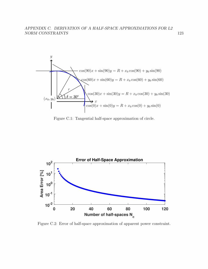
APPENDIX C. DERIVATION OF A HALF-SPACE APPROXIMATIONS FOR L2NORM CONSTRAINTS 123
x
y
(x0, y0)δ = 30◦
cos(0)x+ sin(0)y = R + x0 cos(0) + y0 sin(0)
r
δ = 30◦cos(30)x+ sin(30)y = R + x0 cos(30) + y0 sin(30)
cos(60)x+ sin(60)y = R + x0 cos(60) + y0 sin(60)
cos(90)x+ sin(90)y = R + x0 cos(90) + y0 sin(90)
Figure C.1: Tangential half-space approximation of circle.
0 20 40 60 80 100 120
Number of half-spaces Nc
10-2
10-1
100
101
102
Are
a E
rro
r [%
]
Error of Half-Space Approximation
Figure C.2: Error of half-space approximation of apparent power constraint.
Copyright © 2022 FDOKUMEN

