ONE STEP CLOSER TO FULLY AUTOMATED STRUCTURE INTERPRETATION IN 3D

SEISMIC DATA

by

YIHUAI LOU

BO ZHANG, COMMITTEE CHAIR DELORES M. ROBINSON

YONG ZHANG HERONG ZHENG

XINMING WU

A DISSERTATION

Submitted in partial fulfillment of the requirements for the degree of Doctor of Philosophy

in the Department of Geological Sciences in the Graduate School of

The University of Alabama

TUSCALOOSA, ALABAMA

2020

Copyright Yihuai Lou 2020 ALL RIGHTS RESERVED

ii

ABSTRACT

Seismic structure interpretation is the compulsory step for 3D seismic structure modeling,

stratigraphic features analysis, and 3D reservoir modeling. The modern 3D seismic surveys

usually cover up to hundreds of square kilometers with thousands of inline and crossline vertical

slices. Manual seismic structure interpretation (horizon and fault interpretations) on thousands of

inline and crossline vertical slices is a time-consuming and tedious task. My dissertation focuses

on developing new algorithms and workflows to automatically extract horizon surfaces and fault

surfaces from the 3D seismic data.

Most automatic horizon extraction algorithms are based on the seismic reflector dip

attribute. The quality of extracted horizons is highly affected by the accuracy of the seismic

reflector dip. However, the seismic reflector dip attribute is usually inaccurate near discontinuous

zones such as faults and unconformities. Moreover, the accuracy of an extracted horizon

increases with increasing user interpreted control points. I improve the automatic seismic horizon

interpretation from three aspects: (1) improving the accuracy of the seismic reflector dip

attribute, (2) tracking a horizon using multiple seismic attributes, and (3) automatically

generating control points prior the automatic tracking horizons. The extracted seismic horizons

strictly follow the local seismic reflection events over the whole seismic survey.

Automatic or semi-automatic fault surface construction is still a challenges task although

seismic fault attributes are widely used in assisting seismic fault interpretation in 3D seismic

survey. The staircase and undesired sequence stratigraphic artifacts are the main factors that

ii

hinder researchers from automatically constructing fault surfaces. I improve the automatic

seismic fault interpretation from two aspects: (1) generating a new seismic fault attribute without

staircase and undesired sequence stratigraphic artifacts, and (2) automatically constructing fault

surfaces by analyzing the topological features of the new seismic fault attribute on time and

vertical slices. The proposed fault surface construction workflow successfully constructs fault

surfaces and computes corresponding fault parameters such as fault dip and strike and even

conjugate faults within the seismic survey.

iii

DEDICATION

This dissertation is dedicated to my family.

iv

LIST OF ABBREVIATIONS AND SYMBOLS

DTW Dynamic time warping

GST Gradient structure tensor

IDTW Improved dynamic time warping

MWS Multiple window scanning

PCA Principal component analysis

QC Quality control

RGT Relative geologic time

SNR Signal-to-noise ratio

TWT Two-way traveltime

WPCA Weighted principal component analysis

v

ACKNOWLEDGMENTS

I would like to thank everyone who helped me complete the dissertation research. First, I

want to thank my academic advisor Dr. Bo Zhang for giving me the opportunity to work with

him. This dissertation is impossible to be finished without the help, support, and patient guidance

from Dr. Zhang throughout the past four years. He taught me how to do research, how to make

well-organized slides, and how to organize a technical paper.

I greatly appreciate the support, encouragement, and inspiring comments from my

committee members, Dr. Delores M. Robinson, Dr. Yong Zhang, Dr. Herong Zheng, and Dr.

Xinming Wu. I want to thank the Department of Geological Sciences for providing me the

teaching assistantship funding I have received.

I appreciate the valuable academic comments and help from the faculty and friends in the

AASPI team, Dr. Kurt J. Marfurt, Dr. Jie Qi, and Dr. Tao Zhao. I want to thank the help and

support from my friends, fellow students, and visiting scholars. My special thanks go to Naihao

Liu and Man Lu. I would like to thank Naihao for guidance in code writing. His encouragements

helped me pass through the earliest stage of my research. I would like to thank Man Lu for her

help in teaching, and her companionship brought me lots of joy in my Ph.D. life. I also want to

thank my research group members Hao Wu, Rongchang Liu, and Huijing Fang.

I would like to express my deep gratitude to my parents. I would never have finished my

Ph.D. degree without their endless love, encouragement, and support. Your supports make my

life meaningful, and I hope I have made you proud.

vi

CONTENTS

ABSTRACT .................................................................................................................................... ii

DEDICATION ............................................................................................................................... iii

LIST OF ABBREVIATIONS AND SYMBOLS .......................................................................... iv

ACKNOWLEDGMENTS .............................................................................................................. v

LIST OF FIGURES ........................................................................................................................ x

CHAPTER 1: INTRODUCTION ................................................................................................... 1

REFERENCES ......................................................................................................................................... 6

CHAPTER 2: ACCURATE SEISMIC DIP AND AZIMUTH ESTIMATION USING SEMBLANCE DIP GUIDED STRUCTURE-TENSOR ANALYSIS........................................... 8

2.1 ABSTRACT ........................................................................................................................................ 8

2.2 INTRODUCTION .............................................................................................................................. 9

2.3 DIP ESTIMATION USING MULTIPLE WINDOWS SCANNING............................................... 12

2.4 DIP ESTIMATION BY APPLYSIS TO ANALYTICAL SEISMIC TRACES ............................... 16

2.5 DIP ESTIMATION BY INTEGRATING DISCRETE WINDOW SCANNING AND GST ANALYSIS ............................................................................................................................................. 22

2.6 REAL DATA EXAMPLES .............................................................................................................. 24

2.7 CONCLUSIONS ............................................................................................................................... 34

2.8 REFERENCES ................................................................................................................................. 35

CHAPTER 3: SEISMIC HORIZON PICKING BY INTEGRATING REFLECTOR DIP AND INSTANTANEOUS PHASE ATTRIBUTES .............................................................................. 37

3.1 ABSTRACT ...................................................................................................................................... 37

3.2 INTRODUCTION ............................................................................................................................ 38

3.3 METHOD ......................................................................................................................................... 40

3.3.1 Step one: Patch size and seed definition .................................................................................... 43

3.3.2 Step two: Horizon patches generation and refinement............................................................... 44

vii

3.3.3 Step three: Horizon patches merging ......................................................................................... 48

3.3.4 Step four: Horizon ranking and output....................................................................................... 56

3.4 DISCUSSION ................................................................................................................................... 59

3.5 CONCLUSIONS ............................................................................................................................... 60

3.6 REFERENCES ................................................................................................................................. 62

CHAPTER 4: SIMULATING THE PROCEDURE OF MANUAL SEISMIC HORIZON PICKING ...................................................................................................................................... 64

4.1 ABSTRACT ...................................................................................................................................... 64

4.2 INTRODUCTION ............................................................................................................................ 65

4.3 HORIZON TRACKING WITH THE CONSTRAINT OF CONTROL POINTS ............................ 67

4.4 SEISMIC REFLECTOR’S DIP ESTIMATION USING IMPROVED DYNAMIC TIME WARPING (IDTW) ................................................................................................................................ 69

4.5 LOOP-TIE CHECKING OF AUTOMATICALLY EXTRACTED HORIZON .............................. 72

4.6 THE GENERATION OF LOOP TIE MET HORIZON PATCH ..................................................... 78

4.7 WORKFLOW OF HORIZON PICKING ......................................................................................... 82

4.7.1 Step one: Defining seed seismic traces ...................................................................................... 83

4.7.2 Step two: Producing horizon patches ......................................................................................... 85

4.7.3 Step three: Merging horizon patches.......................................................................................... 86

4.7.4 Step four: Extracting horizon volume ........................................................................................ 90

4.8 THE QUALITY CONTROL (QC) OF EXTRACTED HORIZON ................................................. 92

4.9 CONCLUSIONS ............................................................................................................................... 93

4.10 REFERENCES ............................................................................................................................... 95

CHAPTER 5: SEISMIC FAULT ATTRIBUTE ESTIMATION USING A LOCAL FAULT MODEL ........................................................................................................................................ 97

5.1 ABSTRACT ...................................................................................................................................... 97

5.2 INTRODUCTION ............................................................................................................................ 98

5.3 METHOD ....................................................................................................................................... 100

viii

5.3.1 Coherence computation using a local fault model ................................................................... 101

5.3.2 Fault probability ....................................................................................................................... 107

5.3.3 Fault probability smoothing along the fault plane ................................................................... 110

5.4 RESULTS ....................................................................................................................................... 111

5.4.1 Comparative analysis for a noisy synthetic seismic data ......................................................... 111

5.4.2 Comparative analysis for F3 block seismic survey .................................................................. 112

5.4.3 Comparative analysis for Kerry seismic survey ....................................................................... 114

5.5 DISCUSSION ................................................................................................................................. 116

5.6 CONCLUSIONS ............................................................................................................................. 117

5.7 REFERENCES ............................................................................................................................... 118

CHAPTER 6: FAULT SURFACES CONSTRUCTION THROUGH THE TOPOLOGY ANALYSIS OF SEISMIC FAULT ATTRIBUTES................................................................... 120

6.1 ABSTRACT .................................................................................................................................... 120

6.2 INTRODUCTION .......................................................................................................................... 121

6.3 GENERATING FAULT STICKS USING SEISMIC FAULT ATTRIBUTE ............................... 123

6.3.1 Generating initial fault sticks ................................................................................................... 124

6.3.2 Calculating the orientation of initial fault sticks ...................................................................... 125

6.3.3 Calculating refined fault sticks ................................................................................................ 129

6.4 GROUPING FAULT STICKS ....................................................................................................... 132

6.5 GENERATING FAULT SURFACES THROUGH THE TOPOLOGY ANALYSIS ................... 135

6.5.1 Generating fault surface patches .............................................................................................. 136

6.5.2 Merging fault surface patches .................................................................................................. 143

6.5.3 Calculating fault parameters using 3D WPCA ........................................................................ 146

6.5.4 3D fault surface ........................................................................................................................ 148

6.6 CONCLUSIONS ............................................................................................................................. 150

6.7 REFERENCES ............................................................................................................................... 152

ix

CHAPTER 7: CONCLUSION ................................................................................................... 154

x

LIST OF FIGURES

Figure 2.1. Schematic showing the 2D semblance scanning method (modified from Marfurt, 2006). ............................................................................................................................................ 13

Figure 2.2. A representative inline seismic section with two analysis points (the red and blue crosses). Computed dips of the red and blue crosses are shown in Figure 2.3a and 2.3b, respectively. .................................................................................................................................. 14

Figure 2.3. The computed dip varying with the increment of discrete scanning dips at the analysis points indicated by (a) the red cross and (b) the blue cross in Figure 2.2. ...................... 15

Figure 2.4. The computed dip as a function of discrete candidate analysis windows. (a) The discrete candidate window along the 0° (the traditional GST window). (b) The discrete candidate window along the minimum scanning degree. (c) The discrete candidate window along the dip approximately parallel to the local seismic reflectors. (d) The computed dip for the analysis point. ............................................................................................................................................. 17

Figure 2.5. The computed (a) inline dip and (b) crossline dip at analysis point indicated by the red cross in Figure 2.2. The computed dips are a function of discrete candidate analysis windows computed dip as a function of discrete candidate analysis windows. ........................................... 21

Figure 2.6. The computed (a) inline dip and (b) crossline dip at the analysis point indicated by the blue cross in Figure 2.2. The computed dips are a function of discrete candidate analysis windows. ....................................................................................................................................... 22

Figure 2.7. Workflow for the dip estimation by integrating discrete window scanning and GST analysis. ......................................................................................................................................... 23

Figure 2.8. The representative inline seismic section depicting a salt dome in the black rectangle........................................................................................................................................................ 24

Figure 2.9. Compares the estimated crossline dip of different methods for the inline seismic section in Figure 2.8. Dip estimations based on (a) the semblance scanning method, (b) GST analysis, and (c) our proposed method. ........................................................................................ 25

Figure 2.10. The magnified estimated dip in the blue rectangle in Figure 2.9 overlay on the magnified seismic section in the blue box in Figure 2.8. Dip estimations based on (a) semblance scanning method, (b) GST analysis, and (c) our proposed method. The white arrows in Figure 2.10a indicate estimated dip smears across discontinuous zones. The red arrow in Figure 2.10b indicates the inaccurate dip estimation. The red and white arrows in Figure 2.10c indicate that our method accurately estimates the reflector dip near discontinuous zones. .............................. 26

xi

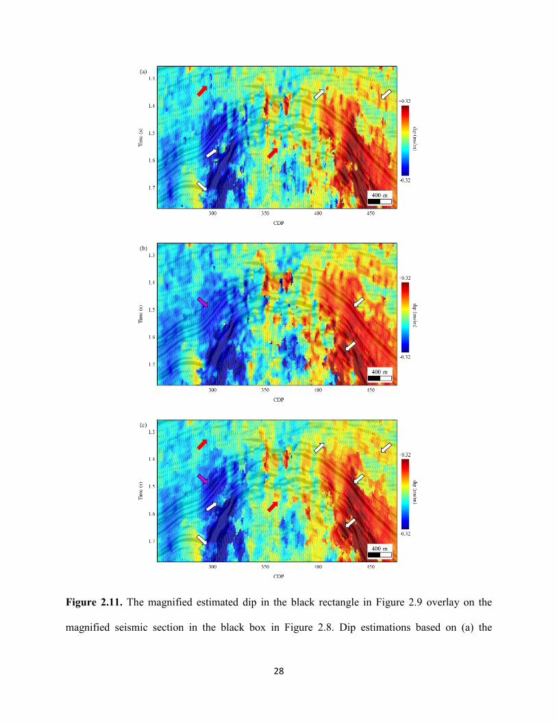
Figure 2.11. The magnified estimated dip in the black rectangle in Figure 2.9 overlay on the magnified seismic section in the black box in Figure 2.8. Dip estimations based on (a) the semblance scanning method, (b) GST analysis, and (c) our proposed method. The white and red arrows in Figure 2.11a indicate inaccurate estimated dips and artifacts, respectively. The purple and white arrows in Figure 2.11b indicate the seismic reflections should have the same color, and almost the same color, respectively. The arrows in Figure 2.11c indicate that our method accurately estimates the reflector dip magnified estimated dip. ................................................... 28

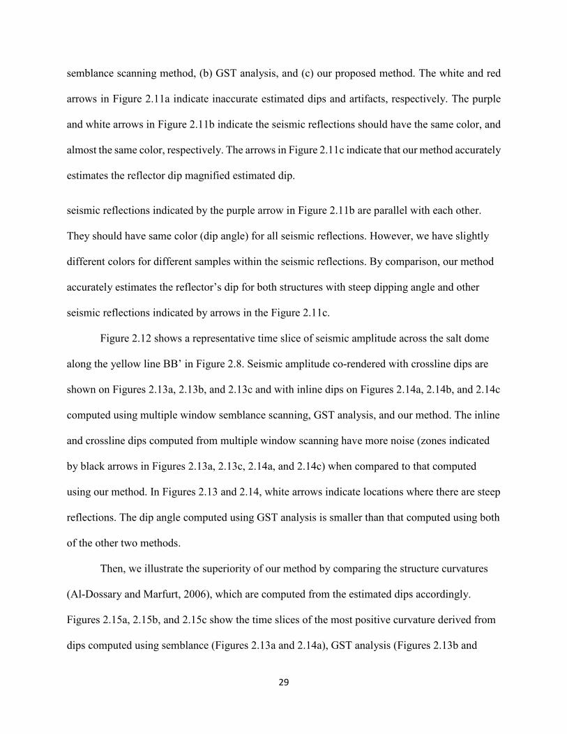
Figure 2.12. The representative time slice seismic data set at 1650 ms. ..................................... 30

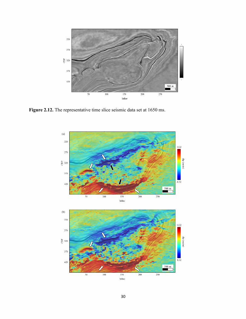
Figure 2.13. Time slice at 1650 ms from the crossline dip volume (equivalent to the time slice in Figure 2.12). Dip estimations based on (a) the semblance scanning method, (b) GST analysis, and (c) our proposed method. The white and black arrows indicate steep reflections and locations with noise, respectively. ................................................................................................................ 31

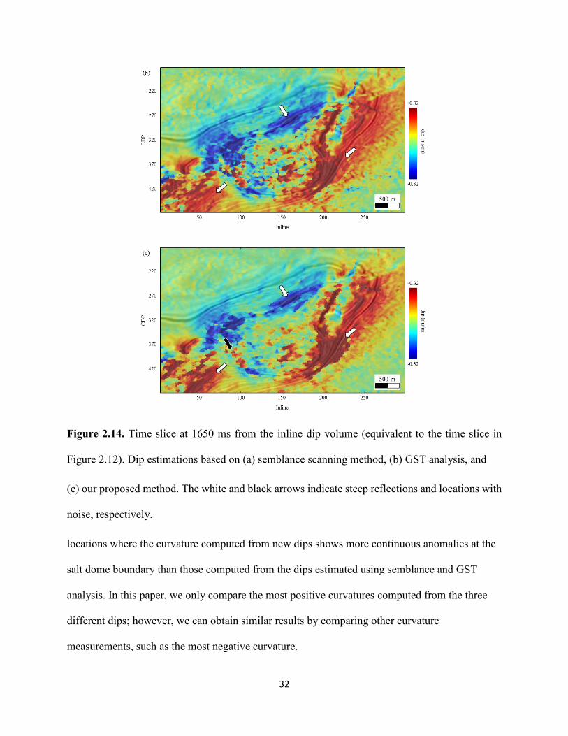
Figure 2.14. Time slice at 1650 ms from the inline dip volume (equivalent to the time slice in Figure 2.12). Dip estimations based on (a) semblance scanning method, (b) GST analysis, and 32

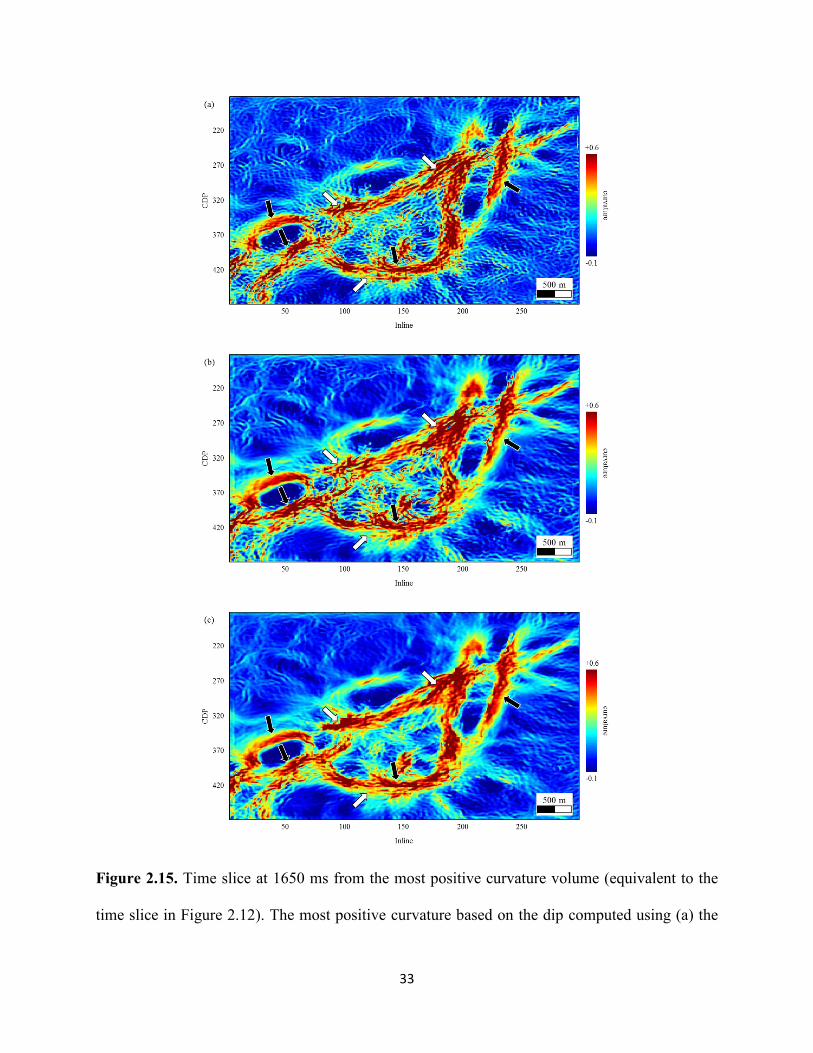
Figure 2.15. Time slice at 1650 ms from the most positive curvature volume (equivalent to the time slice in Figure 2.12). The most positive curvature based on the dip computed using (a) the semblance scanning method, (b) GST analysis, and (c) our proposed method. The white and black arrows indicate representative locations at the salt dome boundary. .................................. 33

Figure 3.1. An automatic tracked horizon using the reflector dip overlaid on (a) a 2D inline seismic section, and overlaid on (b) the corresponding 2D inline instantaneous phase section…41

Figure 3.2. Flowchart showing the automatic horizon tracking and chronostratigraphic relative geologic time (RGT) volume generation based on seismic attributes………………………….. 42

Figure 3.3. The defined overlapping horizon patches………………………………………….. 43

Figure 3.4. The defined seeds (the blue crosses) on a representative inline section…………… 44

Figure 3.5. One representative horizon patch (a) before and (b) after trimming according to the coherence value of the samples on the horizon patch. The t0 represents the two-way traveltime of samples on the patch…………………………………………………………………………….. 46

Figure 3.6. One (a) The tracked horizon patches overlaid on the representative inline instantaneous phase section. (b) The refined horizon patches overlaid on the same inline instantaneous phase section. (c) The magnified tracked horizon patches from the red and blue rectangles in (a and b). Seismic sections 1 and 2 are indicated by the red and blue rectangles in (a), respectively. Seismic sections 3 and 4 are indicated by the red and blue rectangles in (b), respectively……………………………………………………………………………………… 47

Figure 3.7. (a) The target patch and nearby candidate patches before merging any candidate patches. (b) The merging result after merging all of the candidate patches. (c) The interpolated horizon across the seismic survey………………………………………………………………. 49

Figure 3.8. All merged and interpolated horizons overlaid on the representative inline seismic section…………………………………………………………………………………………… 51

xii

Figure 3.9. Geometry analysis between merged and interpolated horizons. (a) Two trough horizons merge together at one end due to the reflections from a nonconformity. (b) Two trough horizons merge together at both ends. (c) The result of three horizons after the geometry analysis………………………………………………………………………………………….. 53

Figure 3.10. The 3D view of two crossing horizons (a) before and (b) after horizon geometry analysis………………………………………………………………………………………….. 55

Figure 3.11. (a) All of the merged horizons after geometry relationship analysis overlaid on the representative inline seismic section. The merged horizons are classified as the selected horizon and invalid horizons. (b) The first output horizon (the yellow line) and remaining horizon patches (the red curves)…………………………………………………………………………. 56

Figure 3.12. The final outputted horizons with the assigned RGT value………………………. 58

Figure 3.13. (a) The computed RGT of the representative inline section. (b) The chair display of the RGT volume using automatically tracked horizons………………………………………….58

Figure 4.1. An automatic tracked horizon with (a) one control point and (b) three control points overlaid on a 2D inline seismic slice……………………………………………………………. 68

Figure 4.2. Two signals and the alignment results. (1) The referred signal. (2) The stretched signal used to align the signal shown in panel 1. The aligned results using (3) DTW and (4) IDTW. The yellow and red arrows indicate modified signal values and severe stretching using DTW, respectively. ....................................................................................................................... 71

Figure 4.3. The calculated reflector dip of the representative sample (yellow dot) using IDTW. Panels 1 and 2 show the referred signal and the stretched signal, respectively. ........................... 72

Figure 4.4. (a) The calculated “left” and “right” reflector dips of the representative sample (yellow dot) located on the referred trace (blue curve) using IDTW. (b) The calculated “right” dip of the red dot and “left” dip of the blue dot located on the target traces (black curves) using IDTW. ........................................................................................................................................... 74

Figure 4.5. A representative example of the loop-tie checking applied in 2D case. The forward tracked horizon with (a) a backward tracked horizon which meets loop-tie checking, and (b) a backward tracked horizon which fails to meet loop-tie checking. (c) The result of accepted and rejected horizons after the loop tie checking. ............................................................................... 77

Figure 4.6. A representative example of the loop-tie checking applied in 3D case. (a) Four representative 2D seismic slices and corresponding tracked horizons before the loop-tie checking. (b) The accepted loop-tie met horizon patch. (c) The rejected loop tie failed horizon patch. ............................................................................................................................................. 79

Figure 4.7. The base map of the seismic survey. ......................................................................... 80

Figure 4.8. The tracked horizon (yellow line) on the crossline slice BB’. .................................. 81

xiii

Figure 4.9. (a) The result after extracting horizons along crossline slices under the constraints of interpretation on inline slice AA’. (b) Before and (c) after cropping the extracted horizon using the loop-tie checking strategy illustrated in Figure 4.6................................................................. 82

Figure 4.10. The workflow showing the proposed horizon volume generation steps. ................ 83

Figure 4.11. The base map of seismic survey with defined seed seismic traces. ........................ 84

Figure 4.12. (a) The defined seeds and (b) loop tie met horizon patches overlaid on the representative inline slice AA’...................................................................................................... 85

Figure 4.13. (a) The selected center horizon patch with the corresponding control point. (b) The selected surrounding candidate horizon patch with the corresponding control point. (c) The center patch after merging the first candidate patch. (d) The center patch after merging all surrounding candidate patches. ..................................................................................................... 88

Figure 4.14. The merged horizon patch in Figure 13d overlaid on the representative inline seismic slice FF’. .......................................................................................................................... 89

Figure 4.15. (a) The center horizon patch after manually merging the isolated horizon patch indicated by the green arrow. (b) The extracted horizon surface over the whole seismic survey. 90

Figure 4.16. (a) The first extracted horizon (blue curve) and iteratively extracted horizons (yellow curves). (b) All extracted horizons on the representative inline slice.............................. 91

Figure 4.17. The extracted horizon surface colored using (a) seismic amplitude and (b) accumulated error.......................................................................................................................... 93

Figure 5.1. Workflow for the new fault attribute based on a local fault model……………….. 101

Figure 5.2. A representative inline seismic section with two analysis points indicated by the yellow and green stars. Candidate fault planes and 2D analysis windows for the yellow star with dip of ........................................................................................................................................... 103

Figure 5.3. The 3D search-based estimation of coherence using our local fault model. ........... 104

Figure 5.4. The 2D coherence results of the yellow star in Figure 5.2 as a function of discrete scanning windows. (a) Cleft + Cright and (b) Cfull. The yellow arrows indicate the maximum Cleft + Cright and its corresponding Cfull. ................................................................................................. 105

Figure 5.5. The 3D coherence results of the yellow star in Figure 5.2. (a) The Cleft + Cright as a function of a set of dip and azimuth. (b) The Cfull as a function of a set of dip and azimuth. The yellow arrows indicate the maximum Cleft + Cright and its corresponding Cfull. .......................... 106

Figure 5.6. The 3D coherence results of the green star in Figure 5.2. (a) The Cleft + Cright as a function of a set of dip and azimuth. (b) The Cfull as a function of a set of dip and azimuth. The yellow arrows indicate the maximum Cleft + Cright and its corresponding Cfull. .......................... 107

Figure 5.7. The statistical analysis of coherence values (Cleft + Cright) for the yellow and green stars in Figure 5.2. (a) The percentage of Cleft + Cright for the yellow star. (b) The percentage of

xiv

Cleft + Cright for the green star. (c) The cumulated frequency of Cleft + Cright for the yellow star. (d) The cumulated frequency of Cleft + Cright for the green star. ....................................................... 109

Figure 5.8. (a) The synthetic noisy image. (b) The result of the semblance-based coherence. (c) The result of the fault attribute generated using our proposed method. The red arrows indicate the fault masked by noise. The blue and green arrows indicate the staircase artifacts and stratigraphic anomalies, respectively. .............................................................................................................. 112

Figure 5.9. Chair diagram showing data from the Netherlands F3 survey: (a) amplitude, clockwise-oriented, (b) semblance-based coherence, and (c) new fault attribute. The red arrows indicate the fault masked by noise. The blue arrows indicate the staircase artifacts. The purple arrows indicate the fault location with discontinuous fault attributes. ....................................... 114

Figure 5.10. Chair diagram showing data from the New Zealand Kerry survey: (a) amplitude, clockwise-oriented, (b) semblance-based coherence, and (c) new fault attribute. The red arrows indicate the fault masked by noise. The blue and green arrows indicate the staircase artifacts and stratigraphic anomalies, respectively. ......................................................................................... 115

Figure 6.1. Chair diagram showing the fault attribute overlaid on corresponding seismic data, which is acquired from the New Zealand Kerry survey……………………………………….. 123

Figure 6.2. The representative example of initial fault stick generation operations. (1) The 2D fault attribute slice. (2) The unanalyzed fault stick. (3) The refined unanalyzed fault stick. (4) The thinned unanalyzed fault stick. (5) The thinned unanalyzed fault stick with furcated pixels indicated by red dots. (6) The initial fault sticks. ....................................................................... 125

Figure 6.3. The calculated fault orientation using (a) all samples in the analysis window and (b) using our proposed method. The first panel shows the analysis point and corresponding analysis window. The second panel shows the samples used to calculated fault orientation. The third panel shows the calculated fault orientation. .............................................................................. 128

Figure 6.4. The refined fault orientation after applying the Kuwahara searching method to the calculated fault orientation in Figure 6.3b. ................................................................................. 129

Figure 6.5. The representative examples of fault stick refinement operations: (a) separating and (b) merging. The first, second and third panels show the initial fault stick, the refined fault orientation, and the refined fault sticks, respectively. ................................................................ 130

Figure 6.6. Chair diagram showing (a) refined fault dip and azimuth and (b) generated vertical and horizontal fault sticks overlaid on the seismic survey. ........................................................ 131

Figure 6.7. Fault sticks grouping workflow. .............................................................................. 133

Figure 6.8. The horizontal fault sticks on a representative time slice. The red arrow indicates the selected horizontal fault stick...................................................................................................... 134

Figure 6.9. The representative example of fault sticks grouping operation. (a) The center stick (blue) and grouped vertical fault sticks (red) in the first grouping round. (b) The new center sticks (blue) and grouped horizontal fault sticks (red). (c) All extracted fault sticks. ................ 135

xv

Figure 6.10. (a) The representative inline slice with three vertical fault sticks. The black and green sticks are mutual exclusion vertical sticks. The representative examples of fault surface patch construction operations (b) without and (c) with mutual exclusion vertical sticks. .......... 137

Figure 6.11. The cartoon of the labeling strategy without mutual exclusion vertical sticks. .... 138

Figure 6.12. The cartoon of the labeling strategy with mutual exclusion vertical sticks. .......... 139

Figure 6.13. The cartoon of the labeling strategy shows the example of stopping merging fault sticks on the current time slice and starting a new fault surface merging on the next time slice...................................................................................................................................................... 140

Figure 6.14. Fault sticks of different fault surfaces on representative time slices after the topological analysis. .................................................................................................................... 142

Figure 6.15. Fault sticks of different fault surface patches on representative inline slice after the topological analysis. .................................................................................................................... 142

Figure 6.16. The automatic merged fault surface patches. ........................................................ 144

Figure 6.17. The fault sticks on representative time slices nearby the crossing time slices of two fault surfaces. .............................................................................................................................. 144

Figure 6.18. (a) The manually merged fault surface patches, and (b) generated fault surfaces. 146

Figure 6.19. (a) The calculated fault azimuth and (b) fault dip overlaid with the generated fault surfaces in Figure 6.18b. ............................................................................................................. 148

Figure 6.20. (a) Generated fault surfaces, and corresponding (b) fault azimuth and (c) fault dip...................................................................................................................................................... 149

1

CHAPTER 1 INTRODUCTION

Horizon and fault interpretations are the main tasks in seismic structure interpretation. To

accelerate the procedure of seismic structure interpretation, researchers have developed

numerous automatic seismic structure interpretation algorithms. However, it is still a challenge to

automatically generate high-quality seismic horizons and faults.

My Ph.D. dissertation concentrates on developing new algorithms and workflows to

accelerate the procedure of the horizon and fault interpretations. My dissertation has two

research objectives: automatically picking seismic horizon and fault surfaces. To achieve my

goals, I first generate a new seismic reflector dip attribute and a new seismic fault attribute to

guarantee the accuracy of extracted seismic horizons and fault surfaces construction. I then

develop algorithms automatically extracting seismic horizons and fault surfaces. The

dissertation consists of seven chapters, an introduction chapter (Chapter 1), five manuscripts

intended to be peer-reviewed journal articles (Chapter 2, Chapter 3, Chapter 4, Chapter 5, and

Chapter 6), and an overall conclusion chapter (Chapter 7).

Horizon interpretation

Most horizon extraction methods are based on seismic reflector dip attributes computed

from seismic data. Lomask et al. (2006) flattened the seismic reflection events using the reflector

dip attribute. Parks (2010) automatically tracked seismic horizons using reflector dip. Wu and

Hale (2015) further improved the stability of automatic horizon picking by adding interpreted

control points. Wu and Fomel (2018) improved the accuracy of extracted horizon picking by

fitting the local reflector dip and correlating the seismic traces on user-defined grids. The

2

instantaneous phase attribute is also used to facilitate horizon interpretation. Stark (2004) first

produced seismic horizons by unwarping the instantaneous phase. Wu and Zhong (2012)

improved the accuracy of seismic horizons near discontinuous zones using the graph cut phase

unwarping method.

Most current automatic horizon extraction algorithms are based on a single seismic

attribute, such as seismic reflector dip or unwrapped instantaneous phases. The quality of the

tracked horizons is highly influenced by the accuracy of the selected seismic attribute. However,

seismic attributes such as reflector dip are usually inaccurate near and across geological features

such as faults and unconformities. Moreover, all current automatic horizon picking algorithms do

not evaluate the accuracy of extracted horizons. The loop-tie is the step checking of the accuracy

of picked horizons in the procedure of manual seismic horizon picking. I propose a set of

strategies to improve the accuracy of automatic seismic horizon interpretation: (1) generating an

accurate seismic reflector dip attribute (chapter 2), (2) extracting seismic horizons using multiple

seismic attributes, including seismic reflector dip, coherence, and instantaneous phase (chapter

3), and (3) developing horizon extracting algorithm, which includes the loop tie checking

(chapter 4).

Chapter 2, entitled “Accurate seismic dip and azimuth estimation using semblance dip

guided structure-tensor analysis”, coauthored by Bo Zhang, Tengfei Lin, Naihao Liu, Hao Wu,

Rongchang Liu, and Danping Cao, was published in Geophysics. This chapter focuses on

developing a new algorithm generating an accurate seismic reflector dip attribute. Currently,

there are two main seismic dip and azimuth estimation methods: (1) the semblance-based

multiple window scanning method, and (2) the gradient structure tensor (GST) analysis.

However, the accuracy of the seismic dip estimated using semblance-based method is affected by

3

the dip of seismic reflectors. The accuracy of the seismic dip estimated using GST analysis is

affected by the analysis window centered at the analysis point. I propose a new algorithm to

overcome the disadvantages of dip estimation using multiple window scanning and GST analysis

by combining and improving these two methods.

Chapter 3, entitled “Seismic horizon picking by integrating reflector dip and

instantaneous phase attributes”, coauthored by Bo Zhang, Tengfei Lin, and Danping Cao, was

published in Geophysics. This chapter focuses on developing a new workflow to automatically

track a horizon for each reflection within the 3D seismic survey. I propose to improve the quality

of picked horizons using multiple seismic attributes, including seismic reflector dip, coherence,

and instantaneous phase. There are four main steps in the proposed workflow: (1) picking

horizon patches using the reflector dip attribute, (2) “trimming” horizon patches using coherence

attribute, (3) refining horizon patches using instantaneous phase attribute, and (4) generating

horizon surfaces by merging horizon patches.

Chapter 4, entitled “Simulating the procedure of manual seismic horizon picking”,

coauthored by Bo Zhang, Huijing Fang, and Danping Cao, is currently under review in

Geophysics. This chapter focuses on developing a new workflow to automatically construct

seismic horizons by simulating the procedure of manual seismic horizon picking. There are three

main steps in the proposed workflow: (1) generating horizon patches, (2) merging horizon

patches, and (3) extract seismic horizon surfaces under the constraints of merged horizon

patches. There are three main steps in generating horizon patches: (1) tracking horizons along

inline seismic slices, (2) tracking horizons along crossline seismic slices, and (3) “cropping”

horizons using the defined loop-tie checking. The loop-tie checking ensures that the

automatically picked horizons patches have the same accuracy with manually picked horizons.

4

Thus, the merged horizon patches can function as the hard constraints for the automatic horizon

picking over the whole seismic survey.

Fault interpretation

Seismic coherence measurements that detect structural discontinuities are normally used

to assist fault interpretation in 3D seismic survey. Marfurt et al. (1998) generated the coherence

algorithm by computing semblance in a suite of windows aligned with candidate reflector dips.

Marfurt et al. (1999) generated the coherence algorithm by using the Eigenstructure of seismic

traces along the reflectors dip. The semblance-based coherence is further improved by

employing a multiple window Kuwahara filtering (Marfurt, 2006). The gradient structure tensor

(GST) is also proposed to detect discontinuities by utilizing the calculated eigenvalues (Bakker

et al., 1999; Fehmers and Hoecker, 2003; Wu, 2017). Hale (2013) computed the fault likelihood

by scanning all possible fault orientations. Researchers have tried to automatically form the

seismic fault surfaces using seismic fault attributes. Zhang et al. (2014) generated fault surfaces

by applying the vein pattern recognition algorithm to the coherence attributes. Wu and Hale

(2016) generated fault surfaces using a linked data structure from 3D seismic images. Wu and

Fomel (2018) proposed the optimal surface voting algorithm to generate fault surfaces, and

calculate corresponding fault dip and azimuth.

Seismic fault attributes provide geoscientists with alternative images of faults, which can

be used to assist seismic fault interpretation. Twenty years after the introduction of coherence,

developing an accurate fault attribute free of artifacts remains an ongoing challenge. Moreover,

seismic fault attributes can only highlight possible fault locations and cannot provide fault

surfaces. I propose a set of strategies to accelerate the procedure of seismic fault interpretation:

(1) generating a new fault attribute without staircase artifacts an undesired stratigraphic

5

anomalies (chapter 5), and (2) constructing seismic fault surfaces through the topology analysis

of the new fault attribute (chapter 6).

Chapter 5, entitled “Seismic Fault Attribute Estimation Using a Local Fault Model”,

coauthored by Bo Zhang, Ruiqi Wang, Tengfei Lin, and Danping Cao, was published in

Geophysics. This chapter focuses on developing a new fault attribute without staircase artifacts.

The proposed algorithm assumes that there exists a fault plane passing through each sample of

our seismic data. The proposed local fault model is composed of the hypothesized fault plane and

an oblique analysis window centered at the analysis sample. The fault plane subdivides the

original oblique analysis window into two sub-windows. The proposed algorithm generates the

new fault attribute without staircase artifacts and undesired stratigraphic anomalies by analyzing

the computed coherence of the two sub-windows and the full analysis window.

Chapter 6, entitled “Fault surfaces construction through the topology analysis of seismic

fault attributes”, coauthored by Bo Zhang, Pan Yong, Huijing Fang, Yijiang Zhang, and Danping

Cao, is currently under review in Geophysics. This chapter focuses on developing a new

workflow to automatically construct fault surfaces within the 3D seismic survey. I propose to

automatically construct fault surfaces by analyzing the topological features of fault attributes.

There are three main steps in the proposed workflow: (1) generating fault sticks, (2) grouping

fault sticks by analyzing the topological relationships, (3) constructing fault surfaces by merging

grouped fault sticks through the topology analysis.

6

REFERENCES

Bakker, P., L. J. van Vliet, and P. W. Verbeek, 1999, Edge-preserving orientation adaptive filtering: IEEE Computer Society Conference on Computer Vision and Pattern Recognition, 1, 535-540.

Fehmers, G. C., and C. F. Höcker, 2003, Fast structural interpretation with structure-oriented filtering: Geophysics, 68(4), 1286-1293.

Hale, D., 2013, Methods to compute fault images, extract fault surfaces, and estimate fault throws from 3D seismic images: Geophysics, 78(2), O33–O43.

Lomask, J., A. Guitton, S. Fomel, J. Claerbout, and A. A. Valenciano, 2006, Flattening without picking: Geophysics, 71(4), P13-P20.

Marfurt, K. J., 2006, Robust estimates of 3D reflector dip and azimuth: Geophysics, 71(4), P29-P40.

Marfurt, K. J., R. L. Kirlin, S. L. Farmer, and M. S. Bahorich, 1998, 3D seismic attributes using a running window semblance-based algorithm: Geophysics, 63(4), 1150-1165.

Marfurt, K. J., V. Sudhakar, A. Gersztenkorn, K. D. Crawford, and S. E. Nissen, 1999, Coherency calculations in the presence of structural dip: Geophysics, 64(1), 104-111

Parks, D., 2010, Seismic image flattening as a linear inverse problem: Master’s thesis, Colorado School of Mines.

Stark, T. J., 2004, Relative geologic time (age) volumes-Relating every seismic sample to a geologically reasonable horizon: The Leading Edge, 23(9), 928-932.

Wu, X., 2017, Structure-, stratigraphy- and fault-guided regularization in geophysical inversion: Geophysical Journal International, 210(1), 184-195.

Wu, X. and D. Hale, 2015, Horizon volumes with interpreted constraints: Geophysics, 80(2), IM21-IM33.

Wu, X. and D. Hale, 2016, 3D seismic image processing for faults: Geophysics, 81(2), IM1-IM11.

Wu, X., and S. Fomel, 2018, Automatic fault interpretation with optimal surface voting: Geophysics, 83(5), O67–O82.

Wu, X., and G. Zhong, 2012, Generating a relative geologic time volume by 3D graph-cut phase unwarping method with horizon and unconformity constraints: Geophysics, 77(4), O21–O34.

Wu, X. and S. Fomel, 2018, Least-squares horizons with local slopes and multi-grid correlations: Geophysics, 84(4), IM29-IM40.

7

Zhang, B., Y. Liu, M. Pelissier, and N. Hemstra, 2014, Semiautomated fault interpretation based on seismic attributes: Interpretation, 2(1), SA11–SA19.

8

CHAPTER 2 ACCURATE SEISMIC DIP AND AZIMUTH ESTIMATION USING SEMBLANCE DIP

GUIDED STRUCTURE-TENSOR ANALYSIS Yihuai Lou1, Bo Zhang1, Tengfei Lin2, Naihao Liu3, Hao Wu1, Rongchang Liu1, and Danping

Cao4

1The University of Alabama, Department of Geological Science. 2Department of Middle East E&P, CNPC.

3Xi’an Jiaotong University, School of Electronic and Information Engineering. 4China University of Petroleum (East China), School of Geoscience.

This paper was published by SEG journal Geophysics in 2019

ABSTRACT

Seismic volumetric dip and azimuth are widely used in assisting seismic interpretation to

depict geological structures such as chaotic slumps, fans, faults, and unconformities. Current

popular dip and azimuth estimation methods include the semblance-based multiple window

scanning method and gradient structure tensor (GST) analysis. However, the dip estimation

accuracy using the semblance scanning method is affected by the dip of seismic reflectors. The

dip estimation accuracy using GST analysis is affected by the analysis window centered at the

analysis point. We proposed a new algorithm to overcome the disadvantages of dip estimation

using multiple window scanning and GST analysis by combining and improving the two

methods. The algorithm first obtains an estimated “rough” dip and azimuth for reflectors using

the semblance scanning method. Then, the algorithm defines a window that is “roughly” parallel

with the local reflectors using the estimated “rough” dip and azimuth. The algorithm next

estimates the dip and azimuth of the reflectors within the analysis window using GST analysis.

To improve the robustness of GST analysis to noise, we employ analytic seismic traces to

compute the GST matrix. The algorithm finally employs Kuwahara window strategy to

9

determine the dip and azimuth of local reflectors. To illustrate the superiority of this algorithm,

we apply it to the F3 block poststack seismic data acquired in the North Sea, Netherlands. The

comparison shows that the seismic volumetric dips estimated using our method more accurately

follow the local seismic reflectors than dips computed from GST analysis and the semblance-

based multiple window scanning method.

INTRODUCTION

The seismic volumetric dip and azimuth, which together reflect the orientations of seismic

events, are important geometric attributes in assisting 3D seismic data interpretation. Four main

categories exist for calculating seismic volumetric dip and azimuth. The first category is based on

the cross-correlation. Bahorich and Farmer (1995) calculated the seismic volumetric dip by

comparing the cross-correlation of a set of windowed seismic data, which was generated using

time-lagging between nearby seismic traces. The second category uses a complex trace analysis to

calculate the volumetric dip. Barnes (1996) and Luo et al. (1996) estimated the seismic dip by

using the partial derivative of the instantaneous phase obtained from 3D complex trace analysis.

To improve the stability of seismic dip estimation, Barnes (2000) smoothed the instantaneous

phase using a weighted average window. Barnes (2007) further estimated the seismic dip by

employing the ratio of smoothed instantaneous wavenumber to smooth instantaneous frequency.

The third category is based on the semblance-based multiple window scanning method. Marfurt et

al. (1998) first calculated semblance between the windowed seismic traces along a set of preset

dips and azimuths and then treated the dip and azimuth pair that has the highest semblance value

as the local reflector’s dip and azimuth. Marfurt (2006) improved the accuracy of dip and azimuth

estimation by using Kuwahara’s multiple-window search. The fourth category is based on the

gradient structure tensor (GST). The seismic volumetric dip and azimuth was estimated by

10

utilizing the eigenvector that corresponds to the largest eigenvalue (Bakker et al., 1999; Fehmers

and Hoecker, 2003). The GST resulted in inaccurate dip estimation when the sampling window

encountered faults and other discontinuous structures. To improve the accuracy of the dip and

azimuth estimation, Luo et al. (2006) used a data-adaptive weighting function to reformulate the

GST. Wang et al. (2018) estimated the dip and azimuth by combining the GST analysis and

Kuwahara’s multiple-window search strategy. Wu and Janson (2017) used directional structure

tensors to estimate the seismic structural and stratigraphic orientations. Other methods, such as

plane-wave destruction (Fomel, 2002), predictive painting (Fomel, 2010), and globally consistent

dip estimation (Aarre, 2010), have been proposed to compute volumetric dip and azimuth.

The volumetric dip and azimuth are widely used to compute other geometric seismic

attributes such as curvatures and similarity/coherence. The volumetric dip and azimuth can be used

to improve the accuracy of the dip-steered coherence near steep structures (Marfurt et al., 1999).

Barnes (2003) used the shaded relief seismic attribute, which combines reflectors dip and azimuth,

to depict small-scale geologic structures. Al-Dossary and Marfurt (2006) used a partial derivative

of reflectors dip to calculate the seismic curvature and further correlate seismic curvatures with

fracture density. Lomask et al. (2006), Wu and Hale (2015; 2016), and Lou and Zhang (2018) used

the reflector dip and azimuth to flatten the seismic reflection events and then generated a relative

geologic time volume based on the flattened seismic volume. Wu and Fomel (2018) used reflection

dips together with multi-grid correlations to calculate least-squares horizons. In addition, the

seismic volumetric dip and azimuth are used for edge-preserving smoothing to detect sharp edges

in seismic data, such as faults and other discontinuous structures (Luo et al., 2002; Qi et al., 2014;

Wu and Guo, 2019). Structure-oriented filtering uses the volumetric dip and azimuth to suppress

noise of both poststack and prestack seismic data and preserve edges of geologic structures

11

(Hoecker and Fehmers, 2002; Zhang et al., 2016; Wu and Guo, 2019). Qi et al. (2016) employed

a structure-oriented Kuwahara filter for seismic facies analysis. The reflector dip and azimuth are

also used to incorporate structural constraints in geophysical inversion problems (Clapp et al.

2004; Wu 2017).

Multiple-window Kuwahara scanning and GST are among the most successful methods

to estimate the dip and azimuth of seismic reflectors. The Kuwahara window search was

developed by Kuwahara et al. (1976) to suppress random noise of image interior textures, but

preserve texture edges. However, the multiple window scanning methods need users to define a

set of dips and azimuths for the dip and azimuth scanning. Unfortunately, the user-defined

increment of discrete candidate dip and azimuth may affect the accuracy of the dip and azimuth

estimation. Computation costs increase with decreasing the interval of dips and azimuths.

However, the accuracy of dip and azimuth estimation may decrease with increasing the interval

of dips and azimuths, especially for the dip reflectors. Thus, it is very difficult to define a

suitable interval of dips and azimuths for the whole seismic survey. GST-based methods treat the

eigenvector (usually the first eigenvector) corresponding to the largest eigenvalue as the dip and

azimuth of the local reflector. However, the correlation between the first eigenvector and dip and

azimuth of local reflectors depends highly on the anisotropy of the windowed seismic image.

The anisotropy of the seismic image is defined as the reflection patterns varying with different

directions. An accurate dip and azimuth estimation can only be obtained if the extracted seismic

events are the dominant linear feature within the analysis window. Thus, it is imperative that the

seismic events within the defined window correspond to the most “dominant” linear feature

(usually the first eigen value and eigen vectors) prior to the estimation of dip and azimuth using

GST analysis. In this paper, we present a new method to estimate the seismic volumetric dip and

12

azimuth robustly by integrating multiple-window Kuwahara scanning and GST analysis. We

begin with generating a set of searching windows centered as the analysis point by rotating the

analysis window along a user-defined dip and azimuth. Then, we calculate the semblance of

seismic data in each analysis window. The window with highest semblance value is the best

window for the following GST analysis. Using the best window, we extract the seismic data and

employ GST analysis to compute the dip and azimuth of seismic data. Finally, we employ the

Kuwahara window search to determine the dip and azimuth of local seismic reflectors. Our

method is applied to the poststack seismic survey in the F3 Block acquired in the North Sea,

Netherlands.

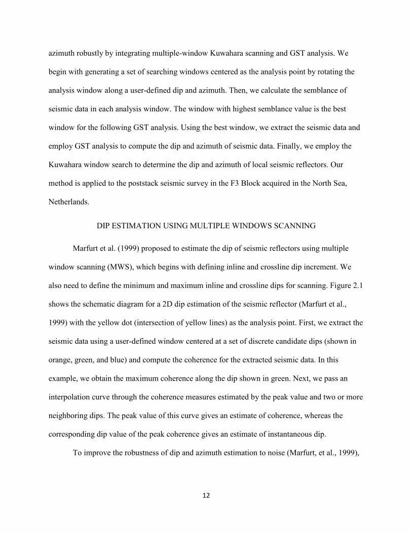
DIP ESTIMATION USING MULTIPLE WINDOWS SCANNING

Marfurt et al. (1999) proposed to estimate the dip of seismic reflectors using multiple

window scanning (MWS), which begins with defining inline and crossline dip increment. We

also need to define the minimum and maximum inline and crossline dips for scanning. Figure 2.1

shows the schematic diagram for a 2D dip estimation of the seismic reflector (Marfurt et al.,

1999) with the yellow dot (intersection of yellow lines) as the analysis point. First, we extract the

seismic data using a user-defined window centered at a set of discrete candidate dips (shown in

orange, green, and blue) and compute the coherence for the extracted seismic data. In this

example, we obtain the maximum coherence along the dip shown in green. Next, we pass an

interpolation curve through the coherence measures estimated by the peak value and two or more

neighboring dips. The peak value of this curve gives an estimate of coherence, whereas the

corresponding dip value of the peak coherence gives an estimate of instantaneous dip.

To improve the robustness of dip and azimuth estimation to noise (Marfurt, et al., 1999),

13

Figure 2.1. Schematic showing the 2D semblance scanning method (modified from Marfurt,

2006).

we employ complex seismic trace ( )yxtF ,, in the following analysis. The complex seismic

trace ( )yxtF ,, is defined as

( ) ( ) ( )t,x,yift,x,yft,x,yF H+= , (2.1)

where Hf is the Hilbert transform of the real seismic trace, f ; t is the two-way travel time; x

and y are the inline and crossline coordinates, respectively. We calculate the coherence ( )lkS ,

for the analysis point in every analysis window using the semblance-based coherence (Marfurt et

al., 1998)

( )( ) ( )

( )[ ] ( )[ ]{ }∑ ∑ +++

∑

∑ ++

∑ +

=+

−= =

+

−= ==

t

tt

t

tt

M

Mm

N

nt

Ht

M

Mm

N

nt

HN

nt

yxmfyxmfN

yxmfyxmflkS

1

20

20

2

10

2

10

ττ

ττ

,,,,

,,,,, , (2.2)

14

where Mt is the half window size in number of samples; k and l are the dip indexes in inline and

crossline directions, respectively; N is the number of seismic traces in the analysis window; τ0 is

the time index corresponding to τ0. We use ( )X to represent ( )yxt ,, in the following analysis.

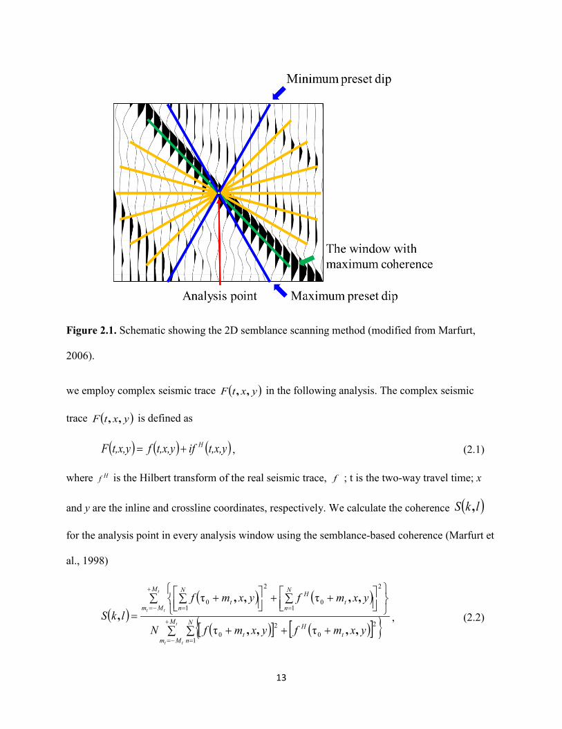
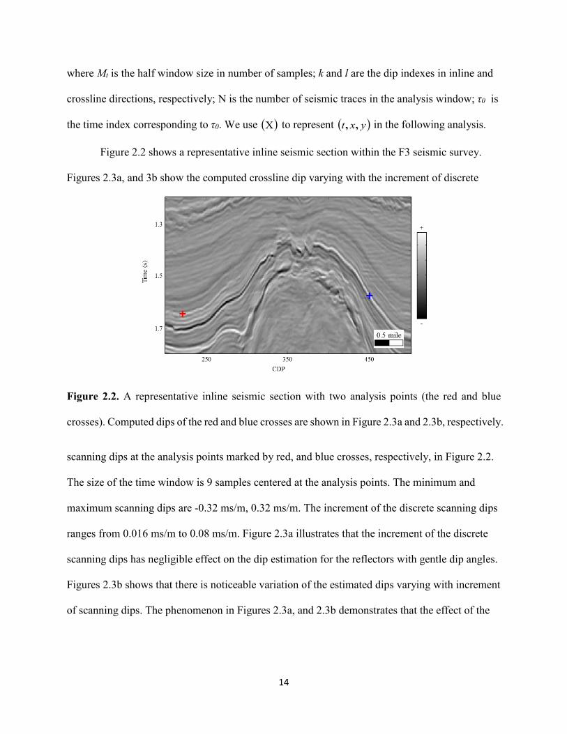
Figure 2.2 shows a representative inline seismic section within the F3 seismic survey.

Figures 2.3a, and 3b show the computed crossline dip varying with the increment of discrete

Figure 2.2. A representative inline seismic section with two analysis points (the red and blue

crosses). Computed dips of the red and blue crosses are shown in Figure 2.3a and 2.3b, respectively.

scanning dips at the analysis points marked by red, and blue crosses, respectively, in Figure 2.2.

The size of the time window is 9 samples centered at the analysis points. The minimum and

maximum scanning dips are -0.32 ms/m, 0.32 ms/m. The increment of the discrete scanning dips

ranges from 0.016 ms/m to 0.08 ms/m. Figure 2.3a illustrates that the increment of the discrete

scanning dips has negligible effect on the dip estimation for the reflectors with gentle dip angles.

Figures 2.3b shows that there is noticeable variation of the estimated dips varying with increment

of scanning dips. The phenomenon in Figures 2.3a, and 2.3b demonstrates that the effect of the

15

increment of discrete scanning dips on the dip estimation for the reflectors increases with

increasing dip angle of the seismic reflectors.

Figure 2.3. The computed dip varying with the increment of discrete scanning dips at the analysis

points indicated by (a) the red cross and (b) the blue cross in Figure 2.2.

16

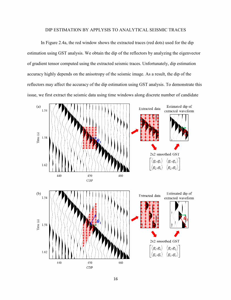
DIP ESTIMATION BY APPLYSIS TO ANALYTICAL SEISMIC TRACES

In Figure 2.4a, the red window shows the extracted traces (red dots) used for the dip

estimation using GST analysis. We obtain the dip of the reflectors by analyzing the eigenvector

of gradient tensor computed using the extracted seismic traces. Unfortunately, dip estimation

accuracy highly depends on the anisotropy of the seismic image. As a result, the dip of the

reflectors may affect the accuracy of the dip estimation using GST analysis. To demonstrate this

issue, we first extract the seismic data using time windows along discrete number of candidate

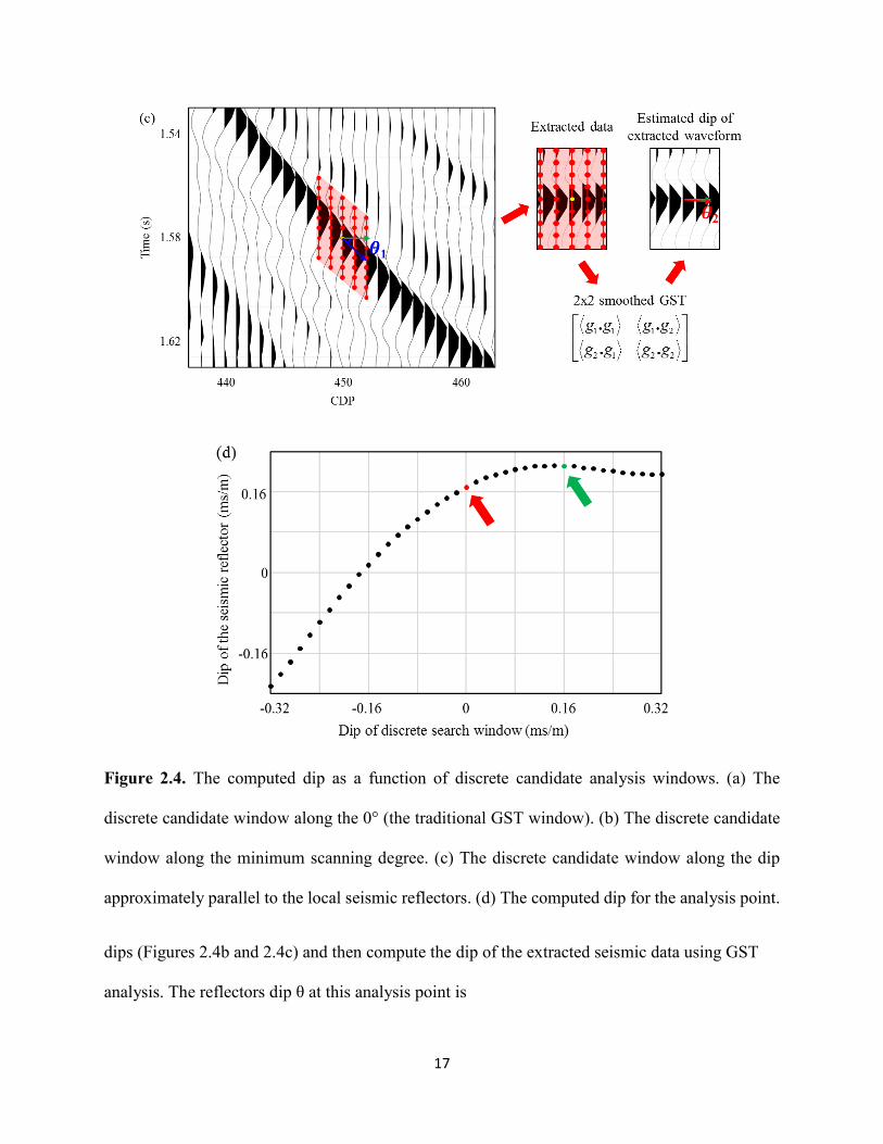
17

Figure 2.4. The computed dip as a function of discrete candidate analysis windows. (a) The

discrete candidate window along the 0° (the traditional GST window). (b) The discrete candidate

window along the minimum scanning degree. (c) The discrete candidate window along the dip

approximately parallel to the local seismic reflectors. (d) The computed dip for the analysis point.

dips (Figures 2.4b and 2.4c) and then compute the dip of the extracted seismic data using GST

analysis. The reflectors dip θ at this analysis point is

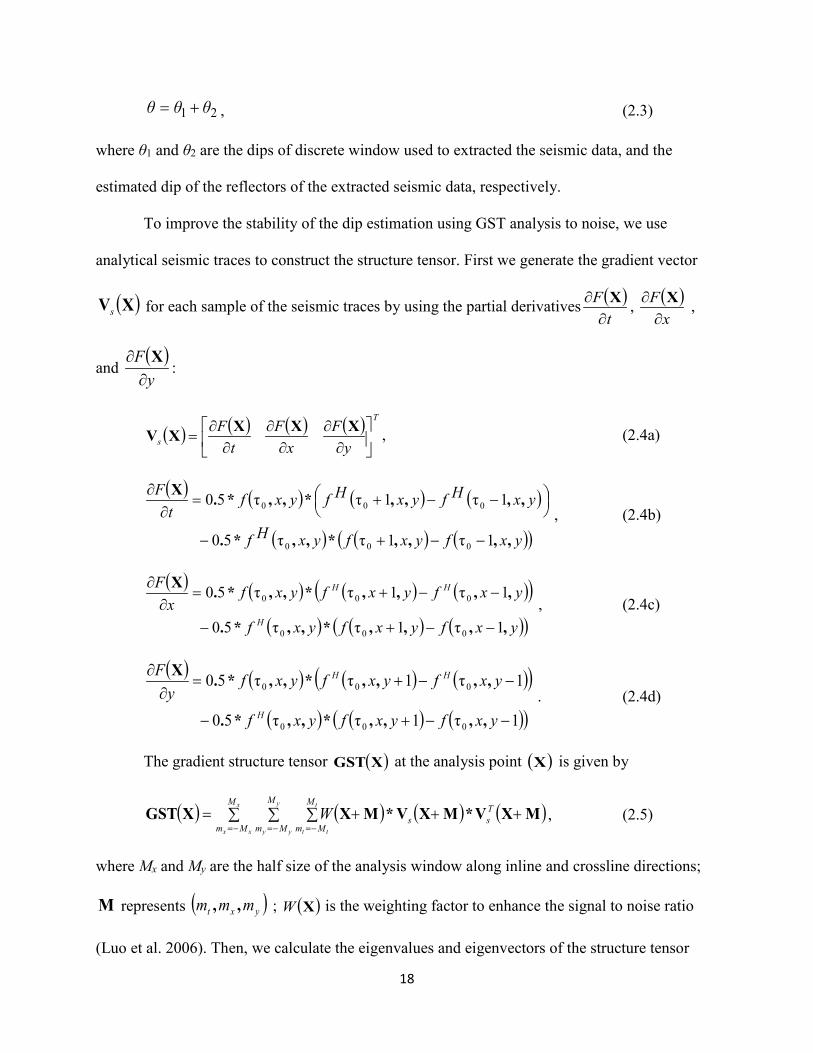
18

21 θθθ += , (2.3)

where θ1 and θ2 are the dips of discrete window used to extracted the seismic data, and the

estimated dip of the reflectors of the extracted seismic data, respectively.

To improve the stability of the dip estimation using GST analysis to noise, we use

analytical seismic traces to construct the structure tensor. First we generate the gradient vector

( )XVs for each sample of the seismic traces by using the partial derivatives ( )t

F∂

∂ X , ( )x

F∂

∂ X ,

and ( )y

F∂

∂ X:

( ) ( ) ( ) ( ) T

s yF

xF

tF

∂

∂∂

∂∂

∂=

XXXXV , (2.4a)

( ) ( ) ( ) ( )

( ) ( ) ( )( )yxfyxfyxHf

yxHfyxHfyxft

F

,,,,*,,*.

,,,,*,,*.X

1τ1ττ50

1τ1ττ50

000

000

−−+−

−−+=

∂∂

, (2.4b)

( ) ( ) ( ) ( )( )( ) ( ) ( )( )yxfyxfyxf

yxfyxfyxfx

F

H

HH

,,,,*,,*.

,,,,*,,*.X

1τ1ττ50

1τ1ττ50

000

000

−−+−

−−+=∂

∂ , (2.4c)

( ) ( ) ( ) ( )( )( ) ( ) ( )( )1τ1ττ50

1τ1ττ50

000

000

−−+−

−−+=∂

∂

yxfyxfyxf

yxfyxfyxfy

F

H

HH

,,,,*,,*.

,,,,*,,*.X . (2.4d)

The gradient structure tensor ( )XGST at the analysis point ( )X is given by

( ) ( ) ( ) ( )MXV*MXV*MXXGST +∑ ∑ ∑ ++=−= −= −=

Ts

M

Mm

M

Mm

M

Mms

x

xx

y

yy

t

tt

W , (2.5)

where Mx and My are the half size of the analysis window along inline and crossline directions;

M represents ( )yxt mmm ,, ; ( )XW is the weighting factor to enhance the signal to noise ratio

(Luo et al. 2006). Then, we calculate the eigenvalues and eigenvectors of the structure tensor

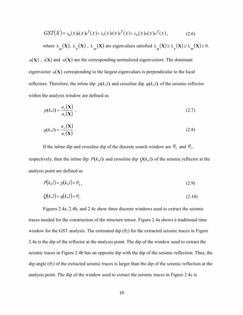
19

( ) ( ) ( ) ( ) ( ) ( ) ( ) ( ) ( ) ( )XwXwXλXvXvXλXuXuXλ Tw

Tv

TuXGST ++= , (2.6)

where ( )Xuλ , ( )Xvλ , ( )Xwλ are eigenvalues satisfied ( ) ( ) ( ) 0λλλ ≥≥≥ XXX wvu .

( )Xu , ( )Xv and ( )Xw are the corresponding normalized eigenvectors. The dominant

eigenvector ( )Xu corresponding to the largest eigenvalues is perpendicular to the local

reflectors. Therefore, the inline dip ),( lkp and crossline dip ),( lkq of the seismic reflector

within the analysis window are defined as

( )( )XX

),(t

x

uu

lkp = , (2.7)

( )( )XX

),(t

y

uu

lkq = . (2.8)

If the inline dip and crossline dip of the discrete search window are kθ and lθ ,

respectively, then the inline dip ),( lkP and crossline dip ),( lkQ of the seismic reflector at the

analysis point are defined as

( ) ( ) kθlkplkP += ,, , (2.9)

( ) ( ) lθlkqlkQ += ,, . (2.10)

Figures 2.4a, 2.4b, and 2.4c show three discrete windows used to extract the seismic

traces needed for the construction of the structure tensor. Figure 2.4a shows a traditional time

window for the GST analysis. The estimated dip (θ2) for the extracted seismic traces in Figure

2.4a is the dip of the reflector at the analysis point. The dip of the window used to extract the

seismic traces in Figure 2.4b has an opposite dip with the dip of the seismic reflection. Thus, the

dip angle (θ2) of the extracted seismic traces is larger than the dip of the seismic reflection at the

analysis point. The dip of the window used to extract the seismic traces in Figure 2.4c is

20

approximately same as the dip of the seismic reflection. Thus, the dip angle (θ2) of the extracted

seismic traces in Figure 2.4c approximately equals to 0 ms/m. Figure 2.4d shows the computed

dip θ at the analysis point labeled by the blue cross shown in Figure 2.2 varying with dips of the

analysis window. The dip value labeled by the green dot in Figure 2.4d is estimated using an

analysis window, which is approximately parallel to the local seismic events. The dip value

labeled by the red dot in Figure 2.4d is estimated using an analysis window which has 0 ms/m

dip angle (the traditional window). Ideally, the estimated dip θ at the analysis point should be a

constant value for all analysis windows if the anisotropy value of seismic images is 0. However,

Figure 2.4d illustrates that we obtain different dip estimations if we use different analysis

windows. Thus, the reflectors dip estimated using GST analysis is highly dependent on how

seismic data are extracted. Figure 2.4d also illustrates that there is negligible variation of dip

values if the analysis windows are approximately parallel with the dip of the local reflectors.

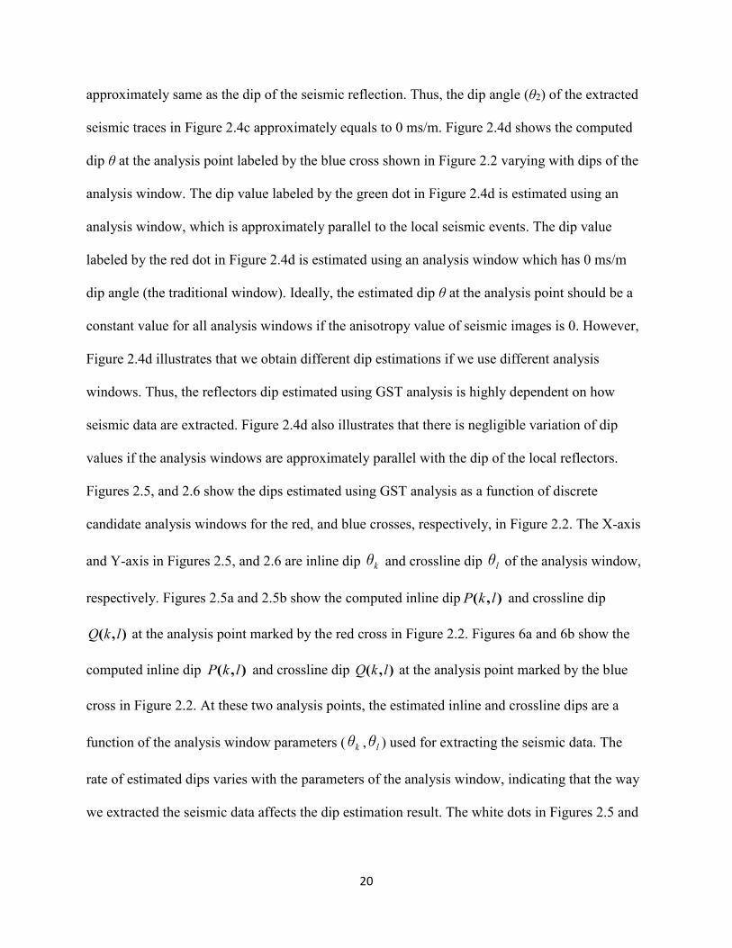
Figures 2.5, and 2.6 show the dips estimated using GST analysis as a function of discrete

candidate analysis windows for the red, and blue crosses, respectively, in Figure 2.2. The X-axis

and Y-axis in Figures 2.5, and 2.6 are inline dip kθ and crossline dip lθ of the analysis window,

respectively. Figures 2.5a and 2.5b show the computed inline dip ),( lkP and crossline dip

),( lkQ at the analysis point marked by the red cross in Figure 2.2. Figures 6a and 6b show the

computed inline dip ),( lkP and crossline dip ),( lkQ at the analysis point marked by the blue

cross in Figure 2.2. At these two analysis points, the estimated inline and crossline dips are a

function of the analysis window parameters ( kθ , lθ ) used for extracting the seismic data. The

rate of estimated dips varies with the parameters of the analysis window, indicating that the way

we extracted the seismic data affects the dip estimation result. The white dots in Figures 2.5 and

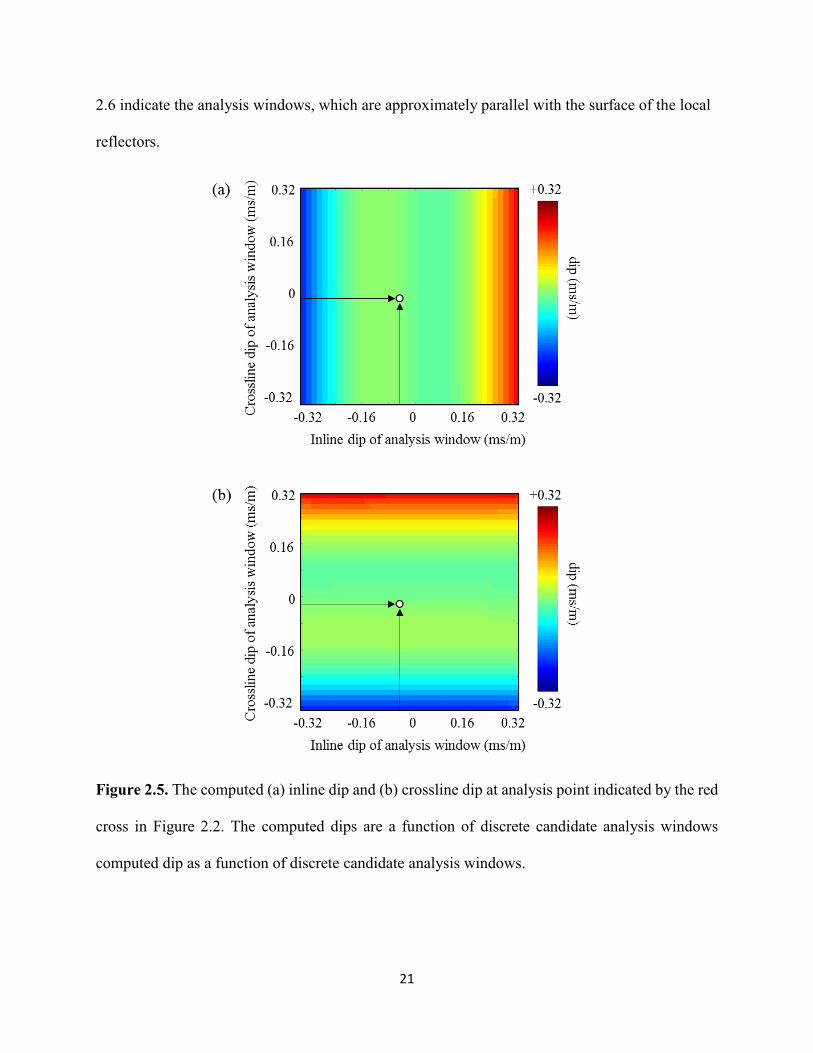
21

2.6 indicate the analysis windows, which are approximately parallel with the surface of the local

reflectors.

Figure 2.5. The computed (a) inline dip and (b) crossline dip at analysis point indicated by the red

cross in Figure 2.2. The computed dips are a function of discrete candidate analysis windows

computed dip as a function of discrete candidate analysis windows.

22

Figure 2.6. The computed (a) inline dip and (b) crossline dip at the analysis point indicated by the

blue cross in Figure 2.2. The computed dips are a function of discrete candidate analysis windows.

DIP ESTIMATION BY INTEGRATING DISCRETE WINDOW SCANNING AND GST

ANALYSIS

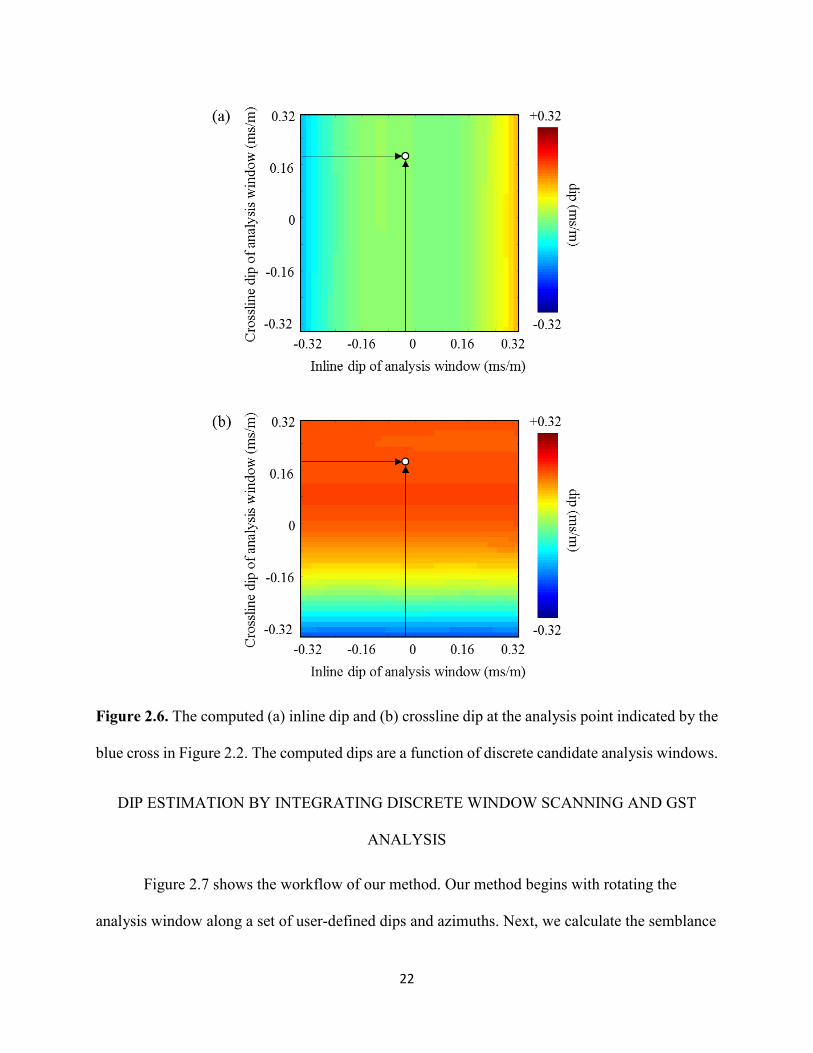
Figure 2.7 shows the workflow of our method. Our method begins with rotating the

analysis window along a set of user-defined dips and azimuths. Next, we calculate the semblance

23

in every analysis window. Considering that the GST analysis may result in inaccurate dip

estimation when the analysis window does not follow the local reflector, we select the window

that is approximately parallel to the local seismic events as the analysis window for GST

analysis. In this paper, we employ the semblance scanning strategy to find the window which is

approximately parallel to the local reflector. Next, we compute the dip and azimuth of the

seismic events within the selected window using GST analysis. Finally, we output the dip,

azimuth, and coherence of the analysis point using Kuwahara searching (Marfurt, 2006).

Figure 2.7. Workflow for the dip estimation by integrating discrete window scanning and GST

analysis.

24

REAL DATA EXAMPLES

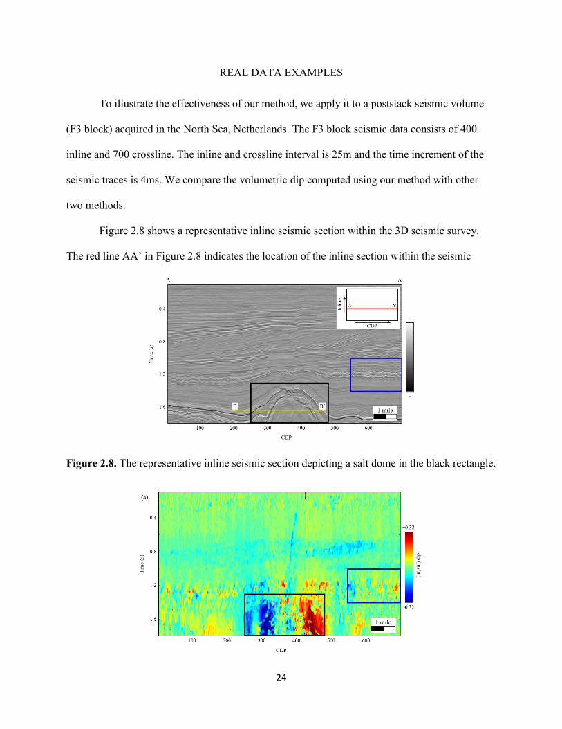
To illustrate the effectiveness of our method, we apply it to a poststack seismic volume

(F3 block) acquired in the North Sea, Netherlands. The F3 block seismic data consists of 400

inline and 700 crossline. The inline and crossline interval is 25m and the time increment of the

seismic traces is 4ms. We compare the volumetric dip computed using our method with other

two methods.

Figure 2.8 shows a representative inline seismic section within the 3D seismic survey.

The red line AA’ in Figure 2.8 indicates the location of the inline section within the seismic

Figure 2.8. The representative inline seismic section depicting a salt dome in the black rectangle.

25

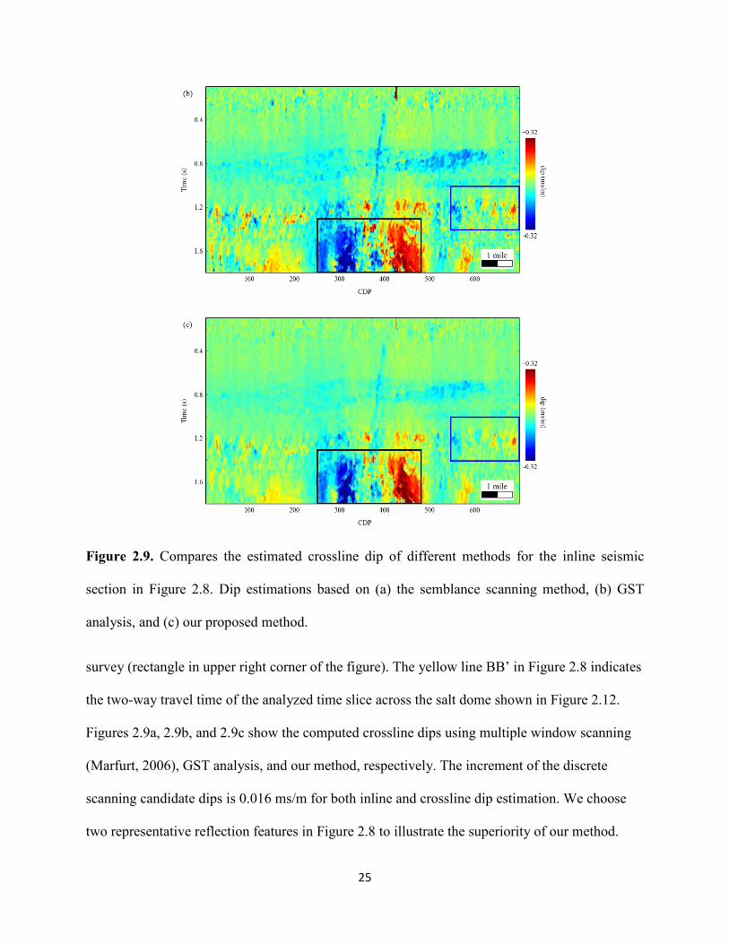
Figure 2.9. Compares the estimated crossline dip of different methods for the inline seismic

section in Figure 2.8. Dip estimations based on (a) the semblance scanning method, (b) GST

analysis, and (c) our proposed method.

survey (rectangle in upper right corner of the figure). The yellow line BB’ in Figure 2.8 indicates

the two-way travel time of the analyzed time slice across the salt dome shown in Figure 2.12.

Figures 2.9a, 2.9b, and 2.9c show the computed crossline dips using multiple window scanning

(Marfurt, 2006), GST analysis, and our method, respectively. The increment of the discrete

scanning candidate dips is 0.016 ms/m for both inline and crossline dip estimation. We choose

two representative reflection features in Figure 2.8 to illustrate the superiority of our method.

26

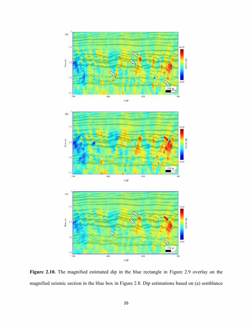
Figure 2.10. The magnified estimated dip in the blue rectangle in Figure 2.9 overlay on the

magnified seismic section in the blue box in Figure 2.8. Dip estimations based on (a) semblance

27

scanning method, (b) GST analysis, and (c) our proposed method. The white arrows in Figure

2.10a indicate estimated dip smears across discontinuous zones. The red arrow in Figure 2.10b

indicates the inaccurate dip estimation. The red and white arrows in Figure 2.10c indicate that our

method accurately estimates the reflector dip near discontinuous zones.

Steep crossline dip angles are present for the seismic reflections within the black rectangle and

“sinusoidal” shapes and chaotic features within the blue rectangle (Figure 2.8). Figures 2.10a,

2.10b, and 2.10c show the zoomed-in seismic amplitude (blue rectangle, Figure 2.8) co-rendered

with the crossline dip computed using multiple window scanning, GST analysis, and our method,

respectively. In Figure 2.10a, the dip computed using the scanning method smears across

discontinuous zones indicated by white arrows. In Figure 2.10b, the estimated dip using GST

analysis has abrupt changes (color changing from red to dark blue) for the seismic reflection

indicated by the red arrow, indicating that the GST based method may give us an inaccurate dip

estimation of seismic reflectors. However, our method accurately estimates the reflectors dip

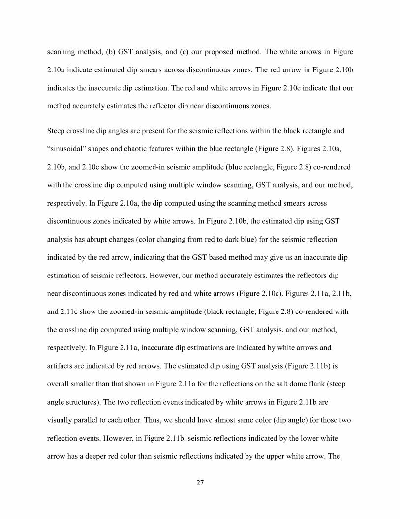
near discontinuous zones indicated by red and white arrows (Figure 2.10c). Figures 2.11a, 2.11b,

and 2.11c show the zoomed-in seismic amplitude (black rectangle, Figure 2.8) co-rendered with

the crossline dip computed using multiple window scanning, GST analysis, and our method,

respectively. In Figure 2.11a, inaccurate dip estimations are indicated by white arrows and

artifacts are indicated by red arrows. The estimated dip using GST analysis (Figure 2.11b) is

overall smaller than that shown in Figure 2.11a for the reflections on the salt dome flank (steep

angle structures). The two reflection events indicated by white arrows in Figure 2.11b are

visually parallel to each other. Thus, we should have almost same color (dip angle) for those two

reflection events. However, in Figure 2.11b, seismic reflections indicated by the lower white

arrow has a deeper red color than seismic reflections indicated by the upper white arrow. The

28

Figure 2.11. The magnified estimated dip in the black rectangle in Figure 2.9 overlay on the

magnified seismic section in the black box in Figure 2.8. Dip estimations based on (a) the

29

semblance scanning method, (b) GST analysis, and (c) our proposed method. The white and red

arrows in Figure 2.11a indicate inaccurate estimated dips and artifacts, respectively. The purple

and white arrows in Figure 2.11b indicate the seismic reflections should have the same color, and

almost the same color, respectively. The arrows in Figure 2.11c indicate that our method accurately

estimates the reflector dip magnified estimated dip.

seismic reflections indicated by the purple arrow in Figure 2.11b are parallel with each other.

They should have same color (dip angle) for all seismic reflections. However, we have slightly

different colors for different samples within the seismic reflections. By comparison, our method

accurately estimates the reflector’s dip for both structures with steep dipping angle and other

seismic reflections indicated by arrows in the Figure 2.11c.

Figure 2.12 shows a representative time slice of seismic amplitude across the salt dome

along the yellow line BB’ in Figure 2.8. Seismic amplitude co-rendered with crossline dips are

shown on Figures 2.13a, 2.13b, and 2.13c and with inline dips on Figures 2.14a, 2.14b, and 2.14c

computed using multiple window semblance scanning, GST analysis, and our method. The inline

and crossline dips computed from multiple window scanning have more noise (zones indicated

by black arrows in Figures 2.13a, 2.13c, 2.14a, and 2.14c) when compared to that computed

using our method. In Figures 2.13 and 2.14, white arrows indicate locations where there are steep

reflections. The dip angle computed using GST analysis is smaller than that computed using both

of the other two methods.

Then, we illustrate the superiority of our method by comparing the structure curvatures

(Al-Dossary and Marfurt, 2006), which are computed from the estimated dips accordingly.

Figures 2.15a, 2.15b, and 2.15c show the time slices of the most positive curvature derived from

dips computed using semblance (Figures 2.13a and 2.14a), GST analysis (Figures 2.13b and

30

Figure 2.12. The representative time slice seismic data set at 1650 ms.

31

Figure 2.13. Time slice at 1650 ms from the crossline dip volume (equivalent to the time slice in

Figure 2.12). Dip estimations based on (a) the semblance scanning method, (b) GST analysis, and

(c) our proposed method. The white and black arrows indicate steep reflections and locations with

noise, respectively.

2.14b), and our method (Figures 2.13c and 2.14c), respectively. The black arrows in Figures

2.15a, 2.15b, and 2.15c indicate representative locations at the salt dome boundary. The smeared

curvature anomalies across the salt dome boundary are indicated by black arrows in Figures

2.15a and 2.15b. However, the curvature anomalies in Figure 2.15c illustrate sharp features at the

salt dome boundary. The white arrows in Figures 2.15a, 2.15b, and 2.15c show the representative

32

Figure 2.14. Time slice at 1650 ms from the inline dip volume (equivalent to the time slice in

Figure 2.12). Dip estimations based on (a) semblance scanning method, (b) GST analysis, and

(c) our proposed method. The white and black arrows indicate steep reflections and locations with

noise, respectively.

locations where the curvature computed from new dips shows more continuous anomalies at the

salt dome boundary than those computed from the dips estimated using semblance and GST

analysis. In this paper, we only compare the most positive curvatures computed from the three

different dips; however, we can obtain similar results by comparing other curvature

measurements, such as the most negative curvature.

33

Figure 2.15. Time slice at 1650 ms from the most positive curvature volume (equivalent to the

time slice in Figure 2.12). The most positive curvature based on the dip computed using (a) the

34

semblance scanning method, (b) GST analysis, and (c) our proposed method. The white and black

arrows indicate representative locations at the salt dome boundary.

CONCLUSIONS

In this paper, we propose a new method to improve the accuracy of volumetric dip

estimation. A proper increment of discrete candidate angles is one of the most important

parameters for the dip estimation using multiple window scanning. The dip estimated using GST

analysis is usually smaller than the dip of seismic reflectors. Our workflow avoids the inaccurate

dip estimation near discontinuous and steep structure zones by integrating the advantages of the

multiple window scanning and GST analysis. We improve the accuracy of dip estimation by

applying GST analysis to the window, which is approximately parallel to the local seismic

reflector. We employ the multiple window scanning method to find the window that is

approximately parallel to the local seismic reflector. Field data examples show that our method

precisely estimates reflectors dip near steep structures. The field data application also

demonstrates that the dip estimated using our method has better anti-noise performance, and the

structure curvature generated using our method precisely highlights the boundary of the salt

dome.

35

REFERENCES

Aarre, V., 2010, Globally consistent dip estimation: SEG Technical Program Expanded Abstracts 2010, 1387-1391.

Al-Dossary, S. and K. J. Marfurt, 2006, 3D volumetric multispectral estimates of reflector curvature and rotation: Geophysics, 71(5), P41-P51.

Bahorich, M., and S. Farmer, 1995, 3D seismic discontinuity for faults and stratigraphic features: The coherence cube: The Leading Edge, 14(10), 1053-1058.

Bakker, P., L. J. van Vliet, and P. W. Verbeek, 1999, Edge-preserving orientation adaptive filtering: IEEE Computer Society Conference on Computer Vision and Pattern Recognition, 1, 535-540.

Barnes, A. E., 1996, Theory of 2-D complex seismic trace analysis: Geophysics, 61(1), 264-272.

Barnes, A. E., 2000, Weighted average seismic attributes: Geophysics, 65(1), 275-285.

Barnes, A. E., 2003, Shaded relief seismic attribute: Geophysics, 68(4), 1281-1285.

Barnes A. E., 2007, A tutorial on complex seismic trace analysis: Geophysics, 72(6), W33-W43.

Clapp, R. G., B. Biondi, and J. F. Claerbout, 2004, Incorporating geologic information into reflection tomography: Geophysics, 69(2), 533–546.

Fehmers, G. C., and C. F. Höcker, 2003, Fast structural interpretation with structure-oriented filtering: Geophysics, 68(4), 1286-1293.

Fomel, S., 2002, Applications of plane-wave destruction filters: Geophysics, 67(6), 1946–1960.

Fomel, S., 2010, Predictive painting of 3-D seismic volumes: Geophysics, 75(4), A25–A30.

Hoecker, C., and G. Fehmers, 2002, Fast structural interpretation with structure-oriented filtering: The Leading Edge, 21(3), 238-243.

Kuwahara, M., K. Hachimura, S. Eiho, and M. Kinoshita, 1976, Processing of RI-angiocardiographic images: Digital processing of biomedical images, 187-202.

Lomask, J., A. Guitton, S. Fomel, J. Claerbout, and A. A. Valenciano, 2006, Flattening without picking: Geophysics, 71(4), P13-P20.

Lou, Y., and B. Zhang, 2018, Automatic horizon picking using multiple seismic attributes: SEG Technical Program Expanded Abstracts 2018, 1683-1687.

Luo, Y., W. G. Higgs, and W. S. Kowalik, 1996, Edge detection and stratigraphic analysis using 3D seismic data: SEG Technical Program Expanded Abstracts 1996, 324-327.

36

Luo, Y., M. Marhoon, S. Al-Dossary, and M. Alfaraj, 2002, Edge-preserving smoothing and applications: The Leading Edge, 21(2), 136–158

Luo, Y., Y. E. Wang, N. M. AlBinHassan, and M. N. Alfaraj, 2006, Computation of dips and azimuths with weighted structural tensor approach: Geophysics, 71(5), V119-V121

Marfurt, K. J., 2006, Robust estimates of 3D reflector dip and azimuth: Geophysics, 71(4), P29-P40.

Marfurt, K. J., R. L. Kirlin, S. L. Farmer, and M. S. Bahorich, 1998, 3D seismic attributes using a running window semblance-based algorithm: Geophysics, 63(4), 1150-1165.

Marfurt, K. J., V. Sudhakar, A. Gersztenkorn, K. D. Crawford, and S. E. Nissen, 1999, Coherency calculations in the presence of structural dip: Geophysics, 64(1), 104-111

Qi, J., B. Zhang, H. Zhou, and K. J. Marfurt, 2014, Attribute expression of fault-controlled karst - Fort Worth Basin, TX: Interpretation, 2(3), SF91–SF110.

Qi, J., T. Lin, T. Zhao, F. Li, and K. J. Marfurt, 2016, Semisupervised multiattribute seismic facies analysis: Interpretation, 4(1), SB91-SB106.

Wang, X., W. Chen, and Z. Zhu, 2018, Robust Seismic Volumetric Dip Estimation Combining Structure Tensor and Multiwindow Technology: IEEE Transactions on Geoscience and Remote Sensing, 99, 1-11.

Wu, X., 2017, Structure-, stratigraphy- and fault-guided regularization in geophysical inversion: Geophysical Journal International, 210(1), 184-195.

Wu, X. and D. Hale, 2015, Horizon volumes with interpreted constraints: Geophysics, 80(2), IM21-IM33.

Wu, X. and D. Hale, 2016, Automatically interpreting all faults, unconformities, and horizons from 3D seismic images: Interpretation, 4(2), T227-T237.

Wu, X. and S. Fomel, 2018, Least-squares horizons with local slopes and multi-grid correlations: Geophysics, 84(4), IM29-IM40.

Wu, X. and Z. Guo, 2019, Detecting faults and channels while enhancing seismic structural and stratigraphic features: Interpretation, 7(1), T155-T166.

Wu, X. and X., Janson, 2017, Directional structure tensors in estimating seismic structural and stratigraphic orientations: Geophysical Journal International, 210(1), 534-548

Zhang, B., T. Lin, S. Guo, O.E. Davogustto, and K.J. Marfurt, 2016, Noise suppression of time-migrated gathers using prestack structure-oriented filtering: Interpretation, 4(2), pp.SG19-SG29.

37

CHAPTER 3 SEISMIC HORIZON PICKING BY INTEGRATING REFLECTOR DIP AND

INSTANTANEOUS PHASE ATTRIBUTES Yihuai Lou1, Bo Zhang1, Tengfei Lin2, Danping Cao3

1The University of Alabama, Department of Geological Science. 2Department of Middle East E&P, Research Institute of Petroleum Exploration & Development,

CNPC. 3China University of Petroleum (East China), School of Geoscience.

This paper was published by SEG journal Geophysics in 2020.

ABSTRACT

Seismic horizons are the compulsory inputs for seismic stratigraphy analysis and 3D

reservoir modeling. Manual interpreting horizons on thousands of vertical seismic slices of 3D

seismic survey is a time consuming task. Automatic horizon interpreting algorithms are usually

based on seismic reflector dip. However, the estimated seismic reflector dip is usually inaccurate

near and across geological features such as unconformities. We propose to improve the quality of

picked horizons using multiple seismic attributes. We assume that seismic horizons follow

reflector dip and the same horizon should have similar instantaneous phase values. We first

generate horizon patches using a reflector dip attribute, which is similar with current methods.

We use seismic coherence attribute as the stop criteria for tracking the horizon within each patch.

Considering the inaccuracy of reflector dip estimates at and near the discontinuous structures

such as fault and unconformities, we use the seismic instantaneous phase attribute to improve the

quality of the generated horizon patches. We generate horizons by merging the residual horizon

patches and only output the best horizon in each iteration. Our method is capable of generating a

horizon for each reflection within the 3D seismic survey and the generated horizons strictly

38

follow the seismic reflections over the whole seismic survey. Finally, each time sample of

seismic traces is assigned a chronostratigraphic relative geologic time value according to the

tracked horizons.

INTRODUCTION

Horizon interpretation is one of the key steps of locating reservoirs and well placement.

Interpreters track horizon surfaces according to the amplitude, phase, and continuity patterns of

seismic events. Horizon picking on a dense grid for a 3D seismic survey is a time-consuming

task. Thus, automating the task will reduce the time consumption. There are four main categories

for the automatic horizon tracking methods.

The first category uses user-interpreted horizons to interpolate a set of separated horizons

(Zeng et al., 1998). Unfortunately, the interpolated horizons usually cannot follow the local

reflectors. The second category is horizon patches method, which is composed of two main

steps. The first step is automatically tracking small horizon surfaces named horizon patches

using seismic attributes on the user-defined subset of the seismic survey. The second step is

merging the horizon patches to form the horizons. Borgos et al. (2003) first used peaks and

troughs of the seismic amplitude to generate horizon patches and then merged the horizon

patches to form a horizon by comparing the similarity of the waveforms of the patches. Monsen

et al. (2007) merged the horizon patches by considering both the waveform attributes and the

topological relationships between the horizon patches. Verney et al. (2008) merged the horizon

patches by considering the geometry relationship between horizon patches. The third category is

based on the dip of seismic reflectors. Lomask et al. (2006) first flattened the seismic reflection

events using the reflector dip and then generated a relative geologic time (RGT) volume based

on the flattened seismic volume. Luo and Hale (2013) first unfaulted a seismic image using fault

39

slip vectors and then unfolded the unfaulted image using seismic normal vectors (perpendicular

to reflection events). Wu and Hale (2015) improved the stability of the horizon picking and

computed a complete horizon volume with the constraint of sets of control points. The fourth

category is based on unwrapping the instantaneous phase of the seismic data. Stark (2004) first

unwrapped the instantaneous phase of seismic data and then produced the RGT volume using the

phase-unwrapped volume. Samples on the same horizon should have the same RGT value. Wu

and Zhong (2012) produced the RGT volume by using the graph-cut phase-unwrapping method.

Unfortunately, unconformity surfaces have to be manually interpreted to constrain the phase

unwrapping (Wu and Hale, 2015). Wu and Fomel (2018) computed horizons across faults by

fitting, in least-squares sense, the horizons with both local slopes and multi-grid correlations of

seismic reflections. Lou and Zhang (2018) employed seismic amplitude, reflector dip and

instantaneous phase to track the horizons.

Selecting proper seismic attributes is very important for seismic interpretation, such as

facies recognition, facies analysis, and structure interpretation (Zhang et al., 2014; Qi et al.,

2016; Qi et al., 2018; Yuan et al., 2018; Lou et al., 2019). Common seismic attributes used for

horizon tracking include seismic phases, reflector dip, and the peak or trough of the seismic

amplitude. Guillon et al. (2013) used the convergence density of seismic reflection events to

highlight periods of non-deposition. Dossi et al. (2015) used the cosine of the instantaneous

phase to detect and characterize reflections in seismic and ground-penetrating radar data. Forte et

al. (2016) used the cosine of the instantaneous phase to detect horizons. Unfortunately, seismic

attributes, such as dip and unwrapped phase, are usually inaccurate at unconformities and near

fault zones. Inaccurate seismic-attribute estimations could further introduce errors in the

automatic horizon picking. The automatically tracked horizons may cross several seismic

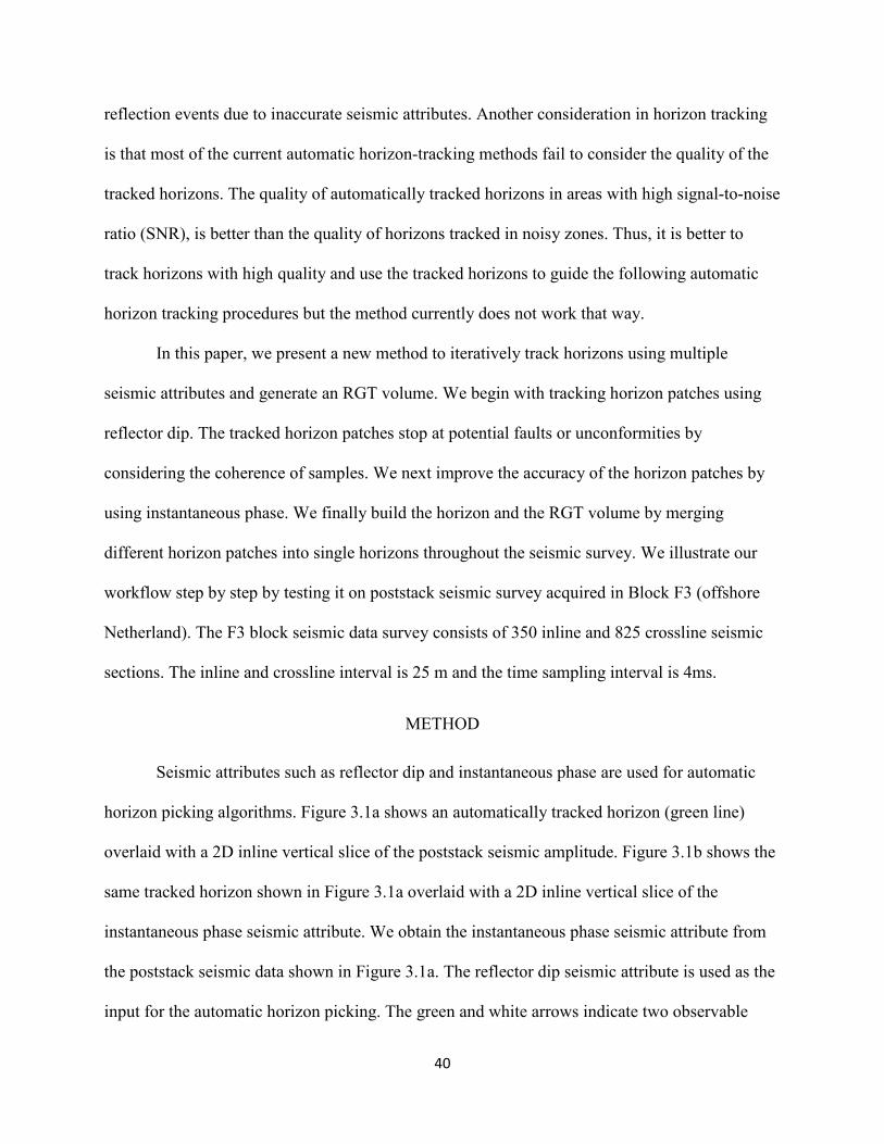
40

reflection events due to inaccurate seismic attributes. Another consideration in horizon tracking

is that most of the current automatic horizon-tracking methods fail to consider the quality of the

tracked horizons. The quality of automatically tracked horizons in areas with high signal-to-noise

ratio (SNR), is better than the quality of horizons tracked in noisy zones. Thus, it is better to

track horizons with high quality and use the tracked horizons to guide the following automatic

horizon tracking procedures but the method currently does not work that way.

In this paper, we present a new method to iteratively track horizons using multiple

seismic attributes and generate an RGT volume. We begin with tracking horizon patches using

reflector dip. The tracked horizon patches stop at potential faults or unconformities by

considering the coherence of samples. We next improve the accuracy of the horizon patches by

using instantaneous phase. We finally build the horizon and the RGT volume by merging

different horizon patches into single horizons throughout the seismic survey. We illustrate our

workflow step by step by testing it on poststack seismic survey acquired in Block F3 (offshore

Netherland). The F3 block seismic data survey consists of 350 inline and 825 crossline seismic

sections. The inline and crossline interval is 25 m and the time sampling interval is 4ms.

METHOD

Seismic attributes such as reflector dip and instantaneous phase are used for automatic

horizon picking algorithms. Figure 3.1a shows an automatically tracked horizon (green line)

overlaid with a 2D inline vertical slice of the poststack seismic amplitude. Figure 3.1b shows the

same tracked horizon shown in Figure 3.1a overlaid with a 2D inline vertical slice of the

instantaneous phase seismic attribute. We obtain the instantaneous phase seismic attribute from

the poststack seismic data shown in Figure 3.1a. The reflector dip seismic attribute is used as the

input for the automatic horizon picking. The green and white arrows indicate two observable

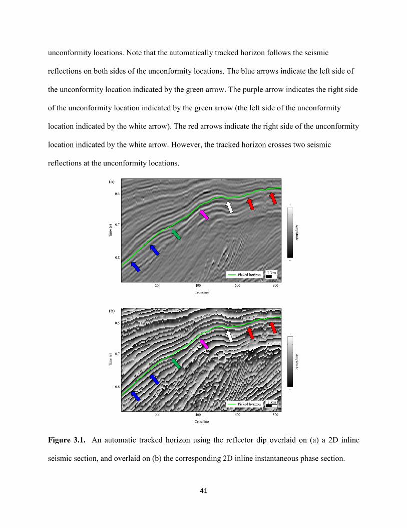
41

unconformity locations. Note that the automatically tracked horizon follows the seismic

reflections on both sides of the unconformity locations. The blue arrows indicate the left side of

the unconformity location indicated by the green arrow. The purple arrow indicates the right side

of the unconformity location indicated by the green arrow (the left side of the unconformity

location indicated by the white arrow). The red arrows indicate the right side of the unconformity

location indicated by the white arrow. However, the tracked horizon crosses two seismic

reflections at the unconformity locations.

Figure 3.1. An automatic tracked horizon using the reflector dip overlaid on (a) a 2D inline

seismic section, and overlaid on (b) the corresponding 2D inline instantaneous phase section.

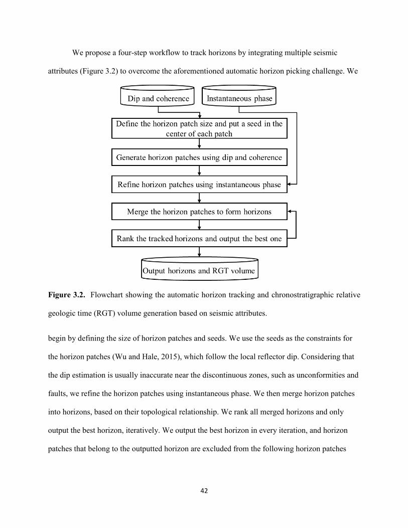
42

We propose a four-step workflow to track horizons by integrating multiple seismic

attributes (Figure 3.2) to overcome the aforementioned automatic horizon picking challenge. We

Figure 3.2. Flowchart showing the automatic horizon tracking and chronostratigraphic relative

geologic time (RGT) volume generation based on seismic attributes.

begin by defining the size of horizon patches and seeds. We use the seeds as the constraints for

the horizon patches (Wu and Hale, 2015), which follow the local reflector dip. Considering that

the dip estimation is usually inaccurate near the discontinuous zones, such as unconformities and

faults, we refine the horizon patches using instantaneous phase. We then merge horizon patches

into horizons, based on their topological relationship. We rank all merged horizons and only

output the best horizon, iteratively. We output the best horizon in every iteration, and horizon

patches that belong to the outputted horizon are excluded from the following horizon patches

43

merging process. We repeat the process of merging, ranking, and outputting until all the horizon

patches belong to a certain horizon.

Step one: Patch size and seed definition

The patch size varies according to the SNR and the complexity of the structure of the

study area. We consider the following criteria in the determination of the size of horizon patches.

The patch size should be small enough to ensure the tracked patches strictly follow the local

reflector dip. The defined patches overlap to facilitate the following process of patches merging.

The topological relationship of the tracked horizon patches within the overlapping zone is used

to avoid the crossing phenomenon in the merging process of horizon patches. The user-defined

patch size of our study case is 36 crossline by 18 inline seismic sections. The size of the

overlapping zone is six crossline by three inline sections. Figure 3.3 shows defined overlapping

Figure 3.3. The defined overlapping horizon patches.

patches for our seismic survey where the red rectangles are the defined horizon patches and the

blue strips are the overlapping zones between defined horizon patches. Every patch is overlapped

with four nearby patches, except patches along the border. Seismic traces used for the seeds

generation (black dots in Figure 3.3) are located at the center of the corresponding horizon

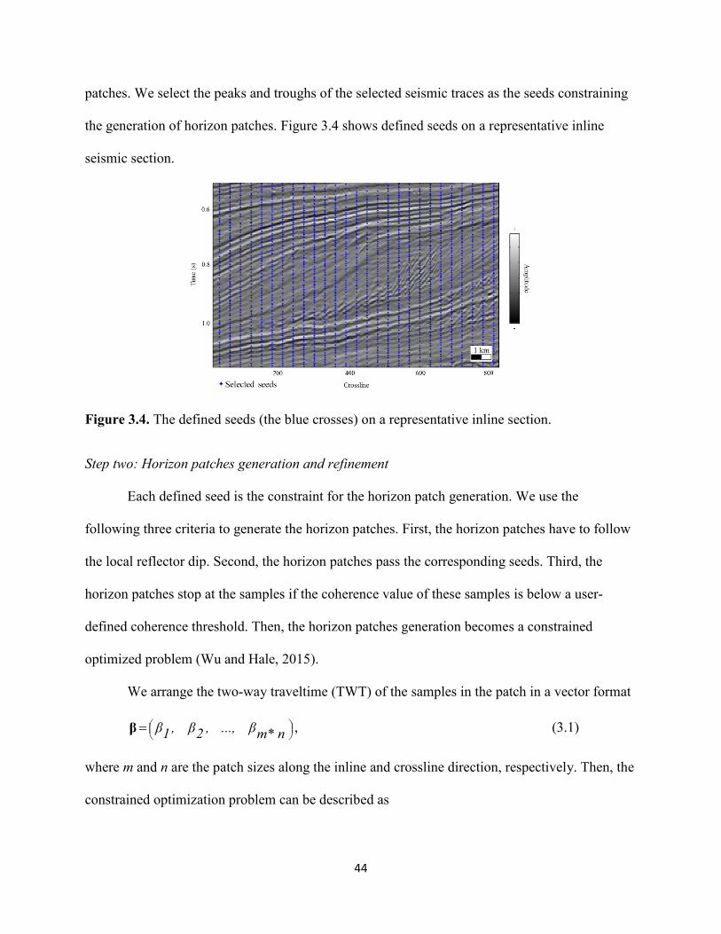
44

patches. We select the peaks and troughs of the selected seismic traces as the seeds constraining

the generation of horizon patches. Figure 3.4 shows defined seeds on a representative inline

seismic section.

Figure 3.4. The defined seeds (the blue crosses) on a representative inline section.

Step two: Horizon patches generation and refinement

Each defined seed is the constraint for the horizon patch generation. We use the

following three criteria to generate the horizon patches. First, the horizon patches have to follow

the local reflector dip. Second, the horizon patches pass the corresponding seeds. Third, the

horizon patches stop at the samples if the coherence value of these samples is below a user-

defined coherence threshold. Then, the horizon patches generation becomes a constrained

optimized problem (Wu and Hale, 2015).

We arrange the two-way traveltime (TWT) of the samples in the patch in a vector format

= n*mβ...,,2β,1ββ , (3.1)

where m and n are the patch sizes along the inline and crossline direction, respectively. Then, the

constrained optimization problem can be described as

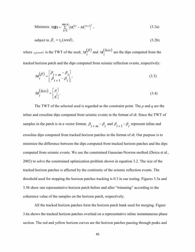
45

Minimize ( ) ( )∑×

=∆−∆=

nm

iS Seis

ii1

2β tt)β( , (3.2a)

subject to )(0 seedts =β , (3.2b)

where )(0 seedt is the TWT of the seed; ( )βit∆ and ( )Seis

it∆ are the dips computed from the

tracked horizon patch and the dips computed from seismic reflection events, respectively:

( )

−+

−+=∆iiimi

i βββββ

1t , (3.3)

( )

=∆

qpSeis

it . (3.4)

The TWT of the selected seed is regarded as the constraint point. The p and q are the

inline and crossline dips computed from seismic events in the format of dt. Since the TWT of

samples in the patch is in a vector format, imi ββ −+ and ii ββ −+1 represent inline and

crossline dips computed from tracked horizon patches in the format of dt. Our purpose is to

minimize the difference between the dips computed from tracked horizon patches and the dips

computed from seismic events. We use the constrained Gaussian-Newton method (Doicu et al.,

2002) to solve the constrained optimization problem shown in equation 3.2. The size of the

tracked horizon patches is affected by the continuity of the seismic reflection events. The

threshold used for stopping the horizon patches tracking is 0.3 in our testing. Figures 3.5a and

3.5b show one representative horizon patch before and after “trimming” according to the

coherence value of the samples on the horizon patch, respectively.

All the tracked horizon patches form the horizon patch bank used for merging. Figure

3.6a shows the tracked horizon patches overlaid on a representative inline instantaneous phase

section. The red and yellow horizon curves are the horizon patches passing through peaks and

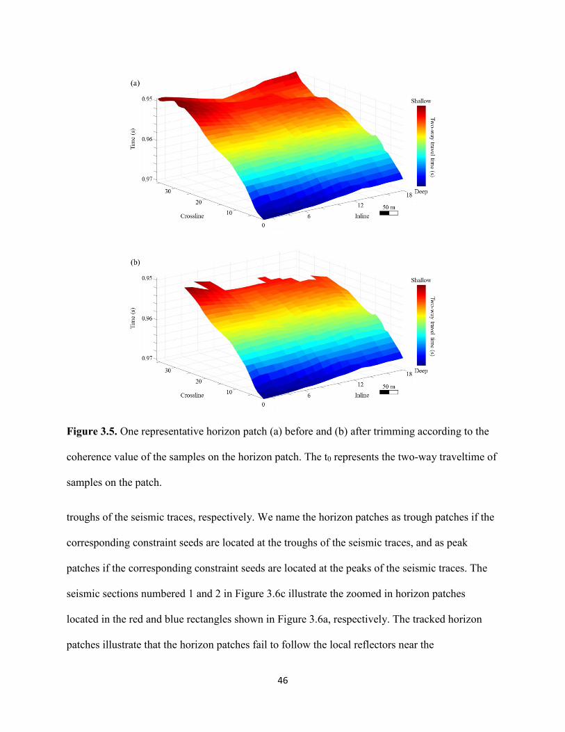
46

Figure 3.5. One representative horizon patch (a) before and (b) after trimming according to the

coherence value of the samples on the horizon patch. The t0 represents the two-way traveltime of

samples on the patch.

troughs of the seismic traces, respectively. We name the horizon patches as trough patches if the

corresponding constraint seeds are located at the troughs of the seismic traces, and as peak

patches if the corresponding constraint seeds are located at the peaks of the seismic traces. The

seismic sections numbered 1 and 2 in Figure 3.6c illustrate the zoomed in horizon patches

located in the red and blue rectangles shown in Figure 3.6a, respectively. The tracked horizon

patches illustrate that the horizon patches fail to follow the local reflectors near the

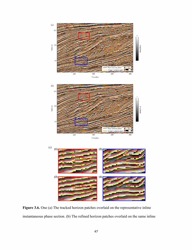
47

Figure 3.6. One (a) The tracked horizon patches overlaid on the representative inline

instantaneous phase section. (b) The refined horizon patches overlaid on the same inline

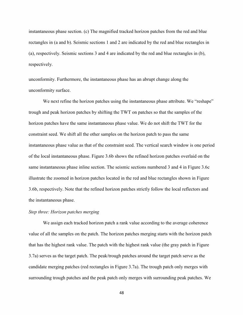
48

instantaneous phase section. (c) The magnified tracked horizon patches from the red and blue

rectangles in (a and b). Seismic sections 1 and 2 are indicated by the red and blue rectangles in

(a), respectively. Seismic sections 3 and 4 are indicated by the red and blue rectangles in (b),

respectively.

unconformity. Furthermore, the instantaneous phase has an abrupt change along the

unconformity surface.

We next refine the horizon patches using the instantaneous phase attribute. We “reshape”

trough and peak horizon patches by shifting the TWT on patches so that the samples of the

horizon patches have the same instantaneous phase value. We do not shift the TWT for the

constraint seed. We shift all the other samples on the horizon patch to pass the same

instantaneous phase value as that of the constraint seed. The vertical search window is one period

of the local instantaneous phase. Figure 3.6b shows the refined horizon patches overlaid on the

same instantaneous phase inline section. The seismic sections numbered 3 and 4 in Figure 3.6c

illustrate the zoomed in horizon patches located in the red and blue rectangles shown in Figure

3.6b, respectively. Note that the refined horizon patches strictly follow the local reflectors and

the instantaneous phase.

Step three: Horizon patches merging

We assign each tracked horizon patch a rank value according to the average coherence

value of all the samples on the patch. The horizon patches merging starts with the horizon patch

that has the highest rank value. The patch with the highest rank value (the gray patch in Figure

3.7a) serves as the target patch. The peak/trough patches around the target patch serve as the

candidate merging patches (red rectangles in Figure 3.7a). The trough patch only merges with

surrounding trough patches and the peak patch only merges with surrounding peak patches. We

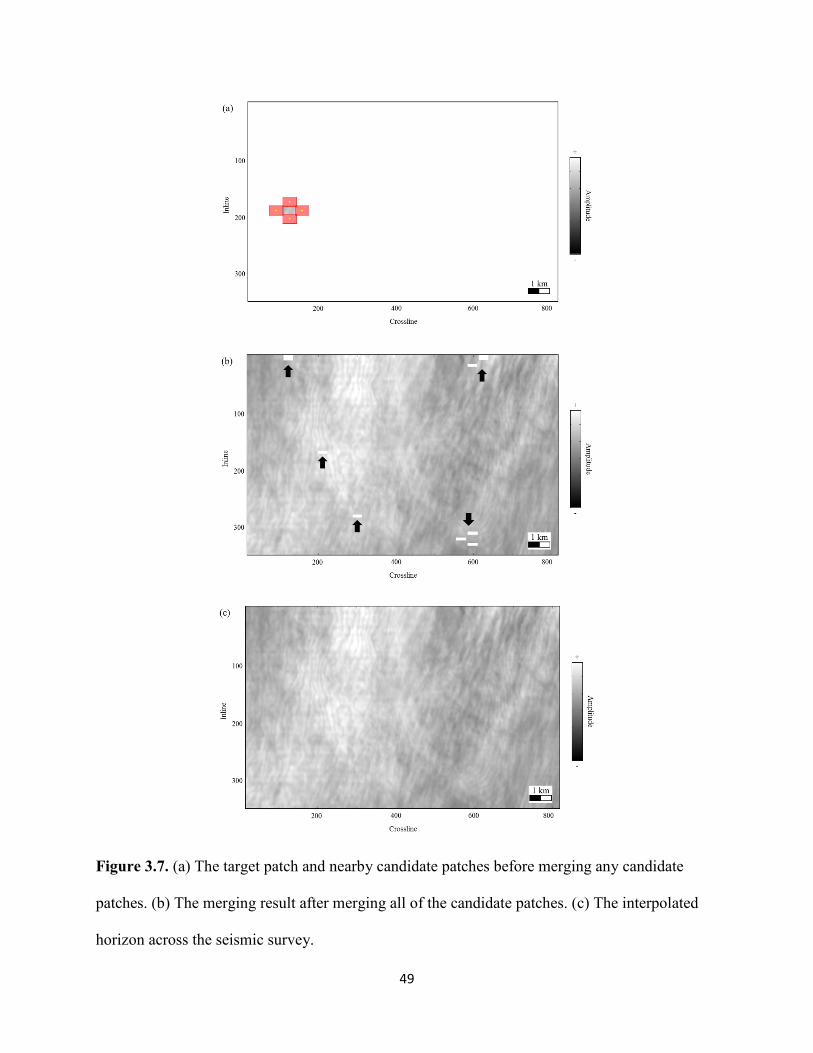
49

Figure 3.7. (a) The target patch and nearby candidate patches before merging any candidate

patches. (b) The merging result after merging all of the candidate patches. (c) The interpolated

horizon across the seismic survey.

50

do not allow a trough patch passing across two merged peak patches, and vice versa. We only

merge one candidate patch each time that has the best match with the target patch.

The seismic traces within the overlapping zone have two tracked TWT (𝑡𝑡0𝑎𝑎 and 𝑡𝑡0𝑏𝑏). The

first tracked 𝑡𝑡0𝑎𝑎 belongs to the target patch while the second 𝑡𝑡0𝑏𝑏 belongs the candidate patch. We

define the matching degree by comparing the similarity S between the seismic amplitude within

the overlapping zone of the target patch and candidate patches. We denote the seismic trace

within the overlapping zone as ( )jif , , where ( )ji, is the location axis of the seismic trace. The

seismic amplitude centered at 𝑡𝑡0𝑎𝑎 and 𝑡𝑡0𝑏𝑏 are defined ( )jifa , and ( )jifb , , respectively. Then, the

similarity between these two seismograms is defined as

( )( ) ( )[ ] ( ) ( )[ ]

( )[ ] ( )[ ] ( )[ ] ( )[ ]∑

∑+

−=

+

−=

+++++++

+++++++

= K

Kk

bHb

bb

aHa

aa

K

Kk

bHb

aHa

bb

aa

jikfjikfjikfjikf

jikfjikfjikfjikf

jiS2

02

02

02

0

200

200

,,,,,,,,

,,,,,,,,

,

ττττ

ττττ

, (3.5)

where K is the half window size in number of samples; 𝜏𝜏0𝑎𝑎 and 𝜏𝜏0𝑏𝑏 are the time indices

corresponding to 𝑡𝑡0𝑎𝑎 and 𝑡𝑡0𝑏𝑏, respectively; and Hf is the Hilbert-transform component of the real

seismic trace f . Then, the similarity between the target and candidate patches is defined as

( )

JI

jiS

S

I

i

J

j

*

,1 1∑∑= == , (3.6)

where I and J are the length and width of overlapping zones of the patches along the inline and

crossline directions, respectively.

After the target path (the gray patch in Figure 3.7a) merges the candidate merging patch

with highest similarity, the new merged horizon patch serves as the target patch and the

surrounding patches serve as the candidate merging patches. We suppose that each horizon

covers the entire seismic survey and our merging process continues until our merged horizon

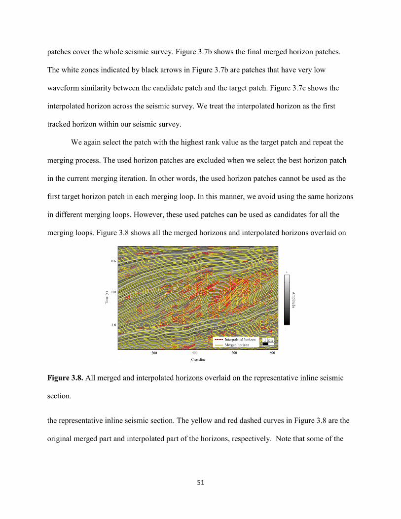
51

patches cover the whole seismic survey. Figure 3.7b shows the final merged horizon patches.

The white zones indicated by black arrows in Figure 3.7b are patches that have very low

waveform similarity between the candidate patch and the target patch. Figure 3.7c shows the

interpolated horizon across the seismic survey. We treat the interpolated horizon as the first

tracked horizon within our seismic survey.

We again select the patch with the highest rank value as the target patch and repeat the

merging process. The used horizon patches are excluded when we select the best horizon patch

in the current merging iteration. In other words, the used horizon patches cannot be used as the

first target horizon patch in each merging loop. In this manner, we avoid using the same horizons

in different merging loops. However, these used patches can be used as candidates for all the

merging loops. Figure 3.8 shows all the merged horizons and interpolated horizons overlaid on

Figure 3.8. All merged and interpolated horizons overlaid on the representative inline seismic

section.

the representative inline seismic section. The yellow and red dashed curves in Figure 3.8 are the

original merged part and interpolated part of the horizons, respectively. Note that some of the

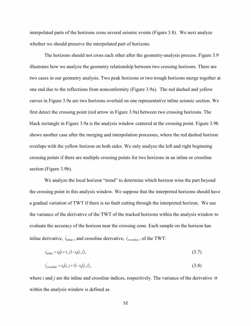
52

interpolated parts of the horizons cross several seismic events (Figure 3.8). We next analyze

whether we should preserve the interpolated part of horizons.

The horizons should not cross each other after the geometry-analysis process. Figure 3.9

illustrates how we analyze the geometry relationship between two crossing horizons. There are

two cases in our geometry analysis. Two peak horizons or two trough horizons merge together at

one end due to the reflections from nonconformity (Figure 3.9a). The red dashed and yellow

curves in Figure 3.9a are two horizons overlaid on one representative inline seismic section. We

first detect the crossing point (red arrow in Figure 3.9a) between two crossing horizons. The

black rectangle in Figure 3.9a is the analysis window centered at the crossing point. Figure 3.9b

shows another case after the merging and interpolation processes, where the red dashed horizon

overlaps with the yellow horizon on both sides. We only analyze the left and right beginning

crossing points if there are multiple crossing points for two horizons in an inline or crossline

section (Figure 3.9b).

We analyze the local horizon “trend” to determine which horizon wins the part beyond

the crossing point in this analysis window. We suppose that the interpreted horizons should have

a gradual variation of TWT if there is no fault cutting through the interpreted horizon. We use

the variance of the derivative of the TWT of the tracked horizons within the analysis window to

evaluate the accuracy of the horizon near the crossing zone. Each sample on the horizon has

inline derivative, 'inlinet , and crossline derivative, '

crosslinet , of the TWT:

( ) ( )jitjittinline ,,1 00' −+= , (3.7)

( ) ( )jitjittcrossline ,1, 00' −+= , (3.8)

where i and j are the inline and crossline indices, respectively. The variance of the derivative σ

within the analysis window is defined as

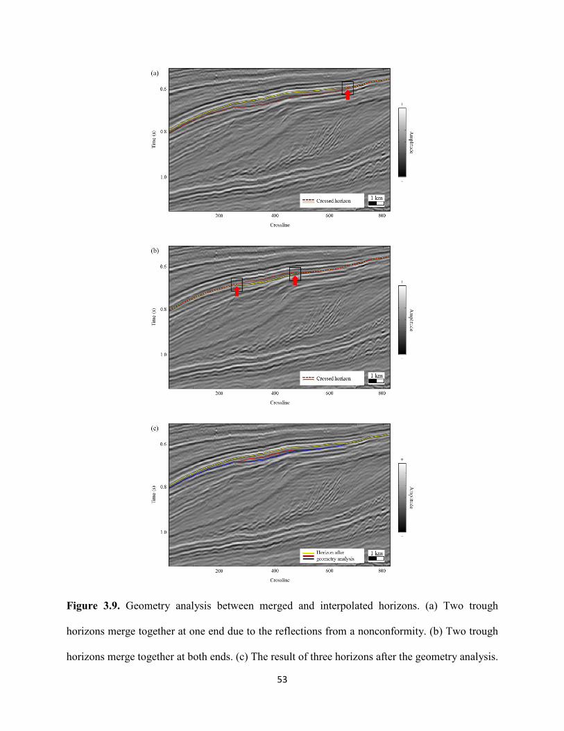
53

Figure 3.9. Geometry analysis between merged and interpolated horizons. (a) Two trough

horizons merge together at one end due to the reflections from a nonconformity. (b) Two trough

horizons merge together at both ends. (c) The result of three horizons after the geometry analysis.

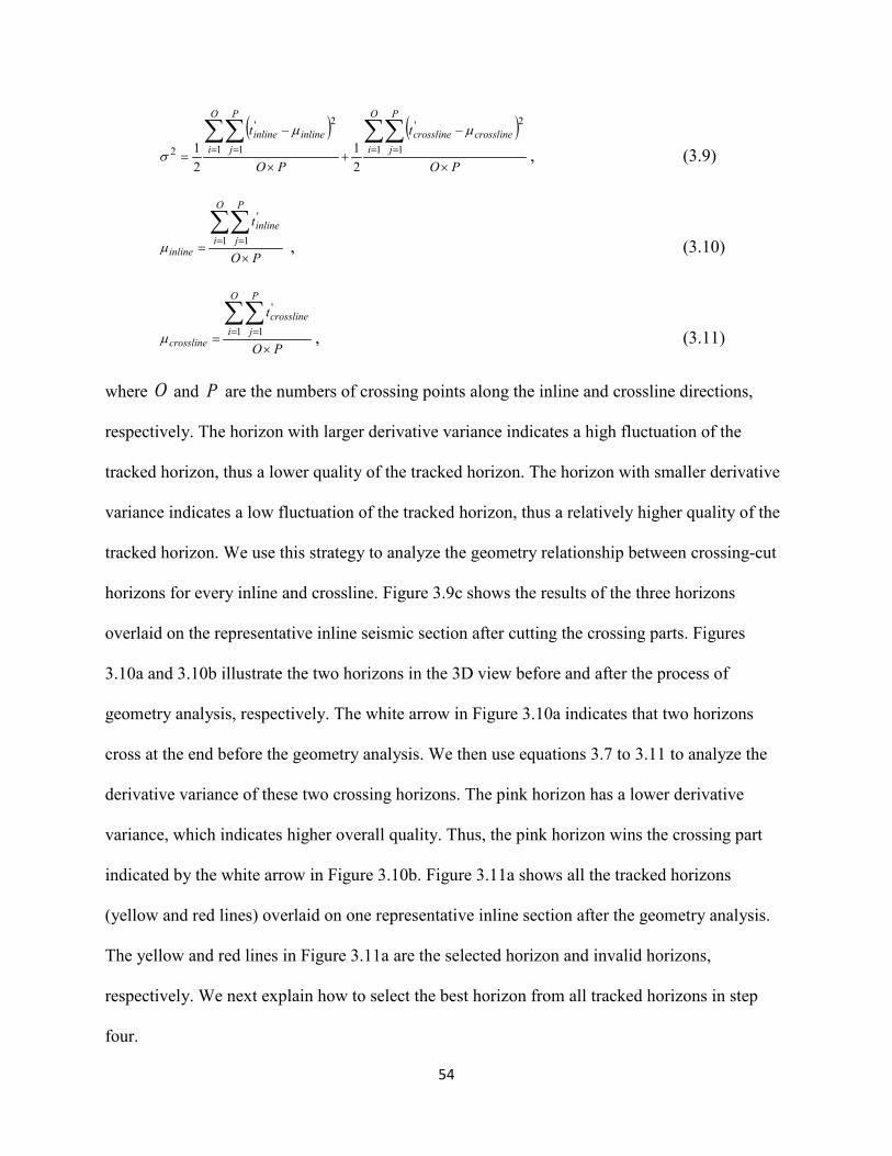
54

( ) ( )PO

t

PO

tO

i

P

jcrosslinecrossline

O

i

P

jinlineinline

×

−

+×

−

=

∑∑∑∑= == = 1 1

2'

1 1

2'

221

21

µµ

σ , (3.9)

PO

tO

i

P

jinline

inline ×=

∑∑= =1 1

'

µ , (3.10)

PO

tO

i

P

jcrossline

crossline ×=

∑∑= =1 1

'

µ , (3.11)

where O and P are the numbers of crossing points along the inline and crossline directions,

respectively. The horizon with larger derivative variance indicates a high fluctuation of the

tracked horizon, thus a lower quality of the tracked horizon. The horizon with smaller derivative

variance indicates a low fluctuation of the tracked horizon, thus a relatively higher quality of the

tracked horizon. We use this strategy to analyze the geometry relationship between crossing-cut

horizons for every inline and crossline. Figure 3.9c shows the results of the three horizons

overlaid on the representative inline seismic section after cutting the crossing parts. Figures

3.10a and 3.10b illustrate the two horizons in the 3D view before and after the process of

geometry analysis, respectively. The white arrow in Figure 3.10a indicates that two horizons

cross at the end before the geometry analysis. We then use equations 3.7 to 3.11 to analyze the

derivative variance of these two crossing horizons. The pink horizon has a lower derivative

variance, which indicates higher overall quality. Thus, the pink horizon wins the crossing part

indicated by the white arrow in Figure 3.10b. Figure 3.11a shows all the tracked horizons

(yellow and red lines) overlaid on one representative inline section after the geometry analysis.

The yellow and red lines in Figure 3.11a are the selected horizon and invalid horizons,

respectively. We next explain how to select the best horizon from all tracked horizons in step

four.

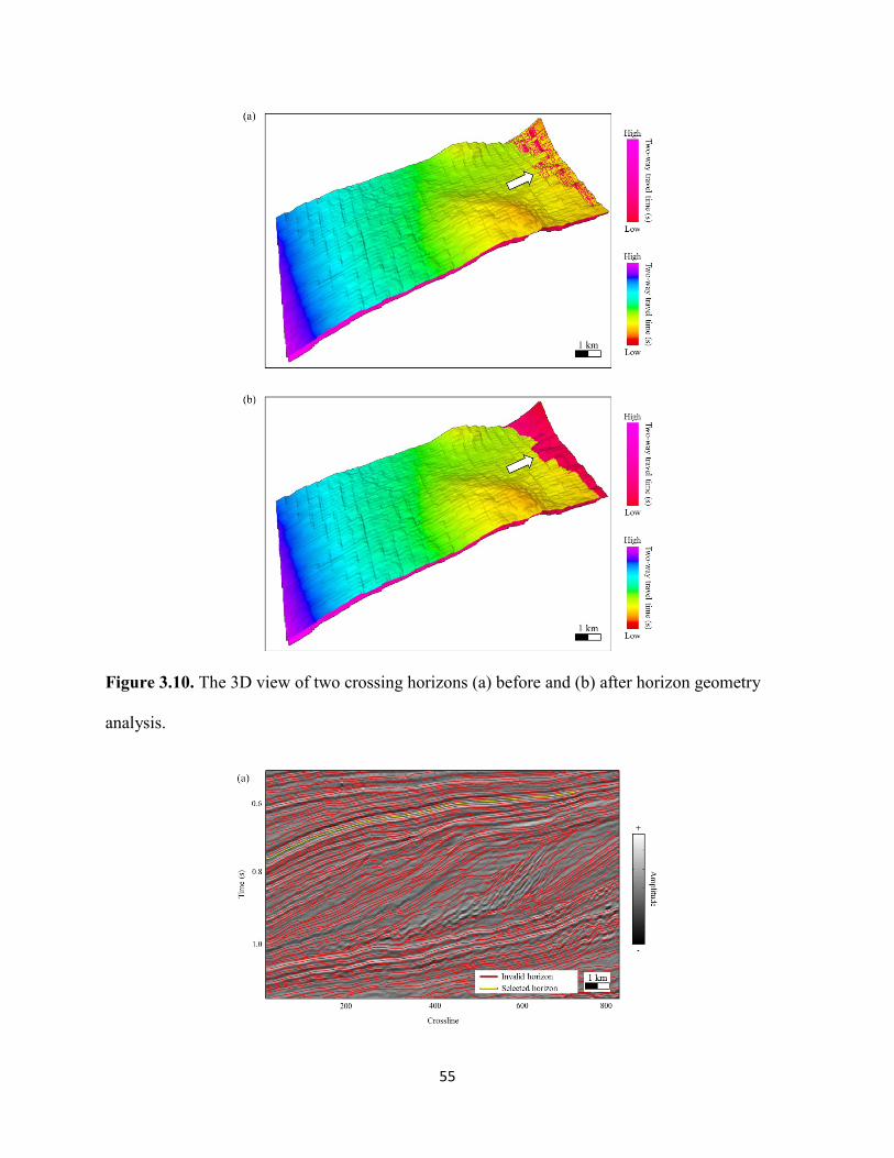
55

Figure 3.10. The 3D view of two crossing horizons (a) before and (b) after horizon geometry

analysis.

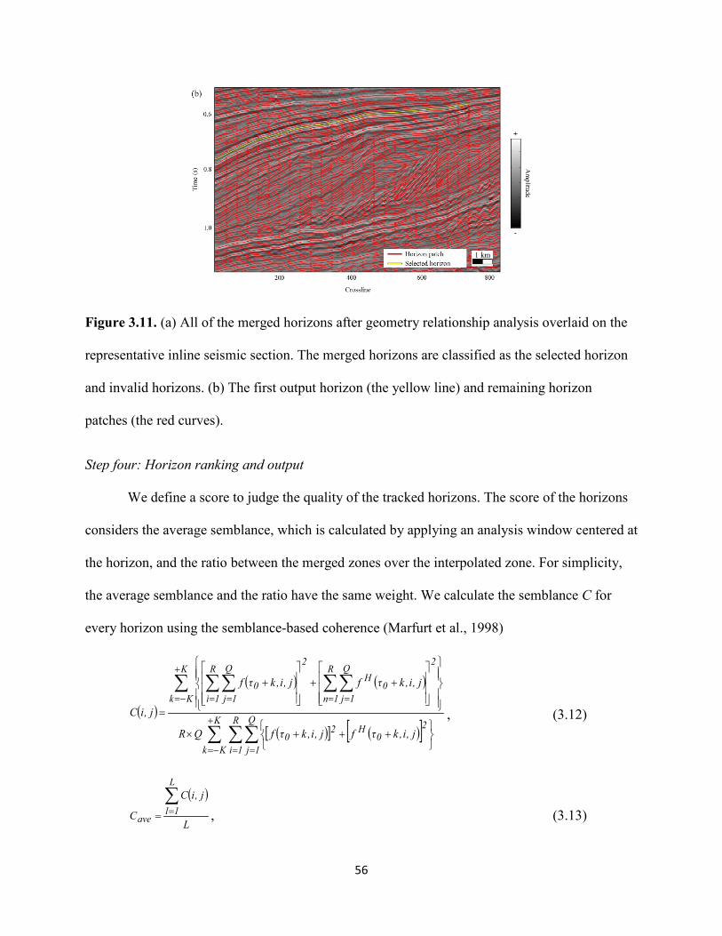
56

Figure 3.11. (a) All of the merged horizons after geometry relationship analysis overlaid on the

representative inline seismic section. The merged horizons are classified as the selected horizon

and invalid horizons. (b) The first output horizon (the yellow line) and remaining horizon

patches (the red curves).

Step four: Horizon ranking and output

We define a score to judge the quality of the tracked horizons. The score of the horizons

considers the average semblance, which is calculated by applying an analysis window centered at

the horizon, and the ratio between the merged zones over the interpolated zone. For simplicity,

the average semblance and the ratio have the same weight. We calculate the semblance C for

every horizon using the semblance-based coherence (Marfurt et al., 1998)

( )

( ) ( )

( )[ ] ( )[ ]∑ ∑∑

∑ ∑∑∑∑

+

−= = =

+

−= = == =

+++×

++

+

=K

Kk

R

1i

Q

1j

20

H20

K

Kk

2R

1n

Q

1j0

H2

R

1i

Q

1j0

j,i,kτfj,i,kτfQR

j,i,kτfj,i,kτf

j,iC , (3.12)

( )

L

j,iC

C

L

1lave

∑== , (3.13)

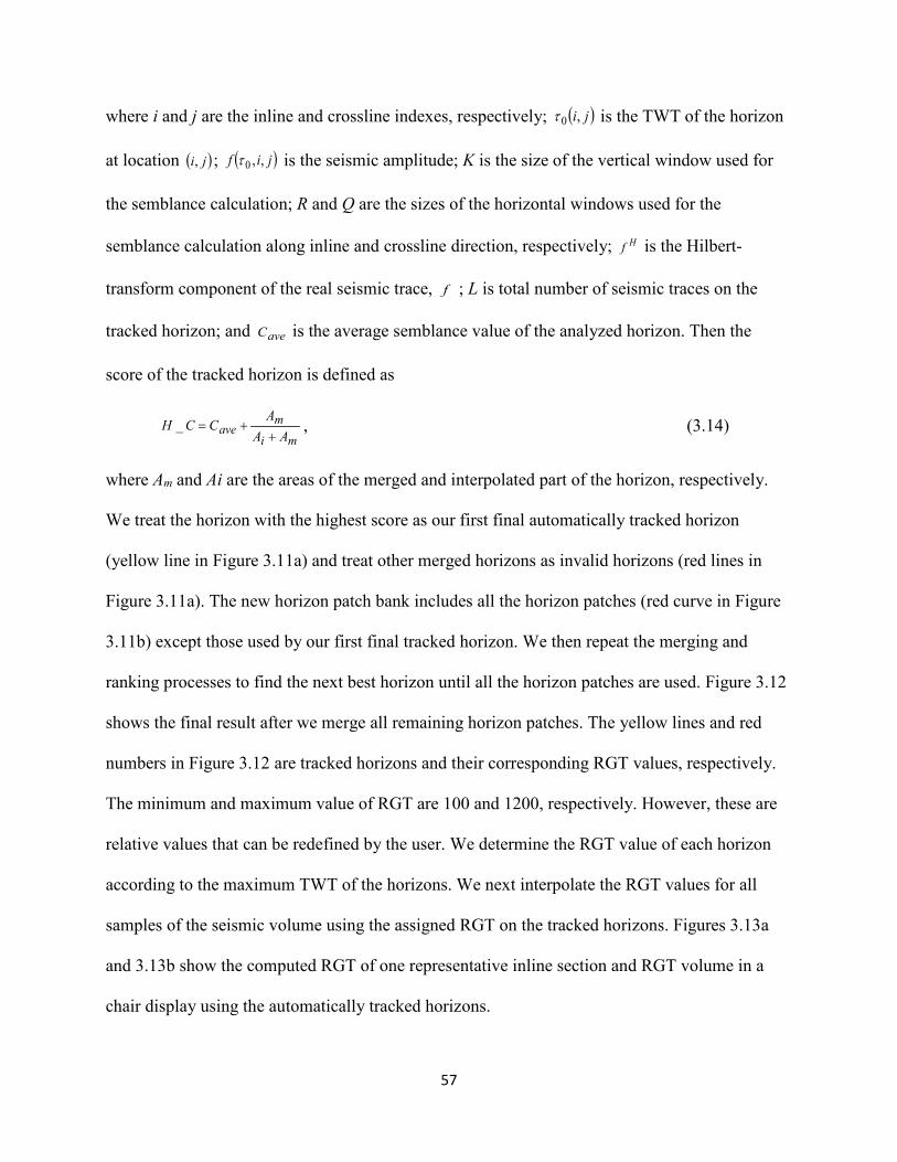
57

where i and j are the inline and crossline indexes, respectively; ( )ji,0τ is the TWT of the horizon

at location ( )ji, ; ( )jif ,,0τ is the seismic amplitude; K is the size of the vertical window used for

the semblance calculation; R and Q are the sizes of the horizontal windows used for the

semblance calculation along inline and crossline direction, respectively; Hf is the Hilbert-

transform component of the real seismic trace, f ; L is total number of seismic traces on the

tracked horizon; and aveC is the average semblance value of the analyzed horizon. Then the

score of the tracked horizon is defined as

mi

mave AA

ACC_H

++= , (3.14)

where Am and Ai are the areas of the merged and interpolated part of the horizon, respectively.

We treat the horizon with the highest score as our first final automatically tracked horizon

(yellow line in Figure 3.11a) and treat other merged horizons as invalid horizons (red lines in

Figure 3.11a). The new horizon patch bank includes all the horizon patches (red curve in Figure

3.11b) except those used by our first final tracked horizon. We then repeat the merging and

ranking processes to find the next best horizon until all the horizon patches are used. Figure 3.12

shows the final result after we merge all remaining horizon patches. The yellow lines and red

numbers in Figure 3.12 are tracked horizons and their corresponding RGT values, respectively.

The minimum and maximum value of RGT are 100 and 1200, respectively. However, these are

relative values that can be redefined by the user. We determine the RGT value of each horizon

according to the maximum TWT of the horizons. We next interpolate the RGT values for all

samples of the seismic volume using the assigned RGT on the tracked horizons. Figures 3.13a

and 3.13b show the computed RGT of one representative inline section and RGT volume in a

chair display using the automatically tracked horizons.

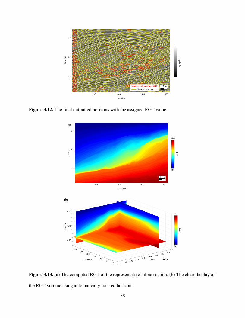
58

Figure 3.12. The final outputted horizons with the assigned RGT value.

Figure 3.13. (a) The computed RGT of the representative inline section. (b) The chair display of

the RGT volume using automatically tracked horizons.

59

DISCUSSION

Our method is based on two assumptions: (1) seismic horizons should follow the reflector

dip, and (2) the same horizon should have similar instantaneous phase values. Both assumptions

have been used to develop algorithms for automated horizons picking. We combine those two

assumptions together for the first time to pick seismic horizons. The value of the instantaneous

phase attribute can be easily affected by the noise. Thus, we suggest to apply a structure oriented

filtering to the seismic data before computing the seismic instantaneous phase, reflector dip, and

coherence attributes. Tracking horizons within a small subdivided seismic survey (patch)

improves the accuracy of the tracked horizons and heavily reduces the size of the matrixes

needed in the optimization process. Our algorithm assumes that the tracked horizon patches after

the refinement process accurately follow the seismic reflections. Thus, the time cost of horizon

patches tracking is the same as for the currently used methods. To make sure that the merged

horizons follow seismic reflections, we only output the best merged horizon in each horizon

merging iteration, and the best merged horizon functions as constraints in the following iterations

of horizon patches merging process. Merging the horizon patches iteration by iteration is the

most time consuming step. The main reason why we need an iterative process is that we do not

have prior information about which seismic reflections will be the “best” reflection in current

horizon tracking iteration. One possible solution of expediting this process is to first rank the

priority of each seismic reflection using signal comparison algorithms such as the dynamic time

warping (DTW) (Sakoe and Chiba, 1978).

A proper horizon patch size and low coherence threshold are the parameters needed for

the generation of horizon patches. The patch size in our application is 36 crosslines by 18 inlines.

We acknowledge that it is challenging to link the patch size with the parameters of seismic

60

survey or seismic data itself. We suggest a two-step workflow to determine the patch size. The

first step is generating the horizon patches according to a set of user defined patch sizes. The

second step is using human judgement to exam whether the generated horizon patches follow

well the local seismic reflections. We choose the largest size whose corresponding horizon

patches follow the local reflections as the patch size in our workflow. We again determine the

low coherence threshold through testing. We choose 0.3 as the low coherence threshold to stop

the horizon tracking process within the defined patch at fault locations. A low similarity value is

needed to determine whether two horizon patches should be merged in the patch merging

process. The value of low similarity is set as the same value with the low coherence threshold

used in the horizon patch generating process.

Picking horizons across faults would be a challenge for our method. Our method is

designed to minimize two objectives: (1) the difference between the dip computed from picked

horizons and dip computed using seismic waveforms, and (2) the phase difference on the picked

horizons between nearby seismic traces. However, the dip of picked horizons at the fault location

is infinite and the dip computed using seismic waveform is inaccurate at the fault location. The

infinite dip and inaccurate dip may hinder us to accurately tracking the horizons across the faults.

One solution is to stop the horizon tracking at the fault location and then align the horizon

patches across the faults using algorithms like dynamic time programming (Sakoe and Chiba,

1978).

CONCLUSIONS

Most current horizon picking methods only use one seismic attribute such as reflector dip

or instantaneous phase as the input to automatically track horizons. The application demonstrates

that the tracked horizon that only used one seismic attribute (reflector dip) may cross several

61

seismic reflections at unconformity locations. The inaccurate computed dip values are

responsible for the inaccurate horizon picking at the unconformity locations. We proposed to

stabilize the horizon picking at the unconformity locations using multiple seismic attributes

(coherence, reflector dip, and instantaneous phase). Interpreters usually produce seismic horizons

by following the peaks or troughs of reflections. Thus, we selected peaks and troughs of seismic

reflections as seeds to constrain the horizon patches generation process. The constrained

Gaussian-Newton method is used by our algorithm to make sure the generated horizon patches

pass through the selected seeds. We tested our method on a field poststack seismic survey data.

We noticed that the same horizon has almost the same instantaneous phase values across the

whole seismic survey. Thus, we successfully corrected the inaccurate two-way travel time of

picked horizon patches in the process of horizon patches generation by using the instantaneous

phase attribute. The refined horizons patches follow very well with the poststack seismic

reflections not only at locations where we have parallel and continuous reflections but also the

unconformity locations where the dip attribute is inaccurate. It is very common that we have very

good SNR for some seismic reflections and low SNR for other seismic reflections even within

the same seismic survey. Thus, it would be beneficial to first pick the seismic reflections with

high SNR and then use those picked horizons as the constraints for the following horizon picking

process. Unfortunately, only picking one horizon each iteration would increase the computation

cost of automatic horizon picking algorithms.

62

REFERENCES

Borgos, H. G., T. Skov, T. Randen, and L. Sonneland, 2003, Automated geometry extraction from 3D seismic data: SEG Technical Program Expanded Abstracts 2003, 1541-1544.

Doicu, A., F. Schreier, and M. Hess, 2002, Iteratively regularized Gauss–Newton method for bound-constraint problems in atmospheric remote sensing: Computer physics communications, 153(1), 59-65.

Dossi, M., E. Forte, and M. Pipan, 2015, Automated reflection picking and polarity assessment through attribute analysis: theory and application to synthetic and real GPR data: Geophysics, 80(5), H23-H35.

Forte, E., M. Dossi, M. Pipan, and A. D. Ben, 2016, Automated phase attribute-based picking applied to reflection seismics: Geophysics, 81(2), V141-V150.

Guillon, S., N. Keskes, J. Gallon, and M. Donias, 2013, Geotime: A 3D automatic tool for chronostratigraphic seismic interpretation and filtering: The Leading Edge, 32(2), 154-159.

Lomask, J., A. Guitton, S. Fomel, J. Claerbout, and A. A. Valenciano, 2006, Flattening without picking: Geophysics, 71(4), P13-P20.

Lou, Y., and B. Zhang, 2018, Automatic horizon picking using multiple seismic attributes: SEG Technical Program Expanded Abstracts 2018, 1683-1687.

Lou, Y., B. Zhang, R. Wang, T. Lin, and D. Cao, 2019, Seismic Fault Attribute Estimation Using a Local Fault Model: Geophysics, 84(4), O73-O80.

Luo, S. and D. Hale, 2013, Unfaulting and unfolding 3D seismic images: Geophysics, 78(4), O45-O56.

Marfurt, K. J., R. L. Kirlin, S. L. Farmer, and M. S. Bahorich, 1998, 3-D seismic attributes using a semblance-based coherency algorithm: Geophysics, 63(4), 1150-1165.

Monsen, E. M., H. G. Borgos, P. L. Guern, and L. Sonneland, 2007, Geological process controlled interpretation based on 3D Wheeler diagram generation: SEG Technical Program Expanded Abstracts 2007, 885-889.

Qi, J., B. Lyu, A. AlAli, G. Machado, Y. Hu, and K. J. Marfurt, 2018, Image processing of seismic attributes for automatic fault extraction: Geophysics, 84(1), O25-O37.

Qi, J., T. Lin, T. Zhao, F. Li, and K. Marfurt, 2016, Semisupervised multiattribute seismic facies analysis: Interpretation, 4(1), SB91-SB106.

Sakoe, H., and S. Chiba, 1978, Dynamic programming algorithm optimization for spoken word recognition: IEEE Transactions on Acoustics, Speech, and Signal Processing, 26, 43–49.

63

Stark, T. J., 2004, Relative geologic time (age) volumes-Relating every seismic sample to a geologically reasonable horizon: The Leading Edge, 23(9), 928-932.

Verney, P., M. Perrin, M. Thonnat, and J. F. Rainaud, 2008, An approach of seismic interpretation based on cognitive vision: 70th EAGE Conference and Exhibition incorporating SPE EUROPEC 2008.

Wu, X. and D. Hale, 2015, Horizon volumes with interpreted constraints: Geophysics, 80(2), IM21-IM33.

Wu, X., and G. Zhong, 2012, Generating a relative geologic time volume by 3D graph-cut phase unwrapping method with horizon and unconformity constraints: Geophysics, 77(4), O21–O34.

Wu, X., and S. Fomel, 2018, Least-squares horizons with local slopes and multi-grid correlations, Geophysics, 83(4), IM29–IM40.

Yuan, S., Y. Su, T. Wang, J. Wang, and S. Wang, 2018, Geosteering phase attributes: A new detector for the discontinuities of seismic images: IEEE Geoscience and Remote Sensing Letters, 99, 1-5.

Zeng, H., M. M. Backus, K. T. Barrow, and N. Tyler, 1998, Stratal slicing, part I: realistic 3-D seismic model: Geophysics, 63(2), 502-513.

Zeng, H., S. C. Henry, and J. P. Riola, 1998, Strata slicing; Part II, Real 3-D seismic data: Geophysics, 63(2), 514–522.

Zhang, B., Y. Liu, M. Pelissier, and N. Hemstra, 2014, Semiautomated fault interpretation based on seismic attributes: Interpretation, 2(1), SA11-SA19.

64

CHAPTER 4 SIMULATING THE PROCEDURE OF MANUAL SEISMIC HORIZON PICKING

Yihuai Lou1, Bo Zhang1, Huijing Fang2 and Danping Cao3 1The University of Alabama, Department of Geological Science.

2China University of Petroleum (Beijing), College of Geosciences. 3China University of Petroleum (East China), School of Geoscience.

This paper was submitted to SEG journal Geophysics in 2020.

ABSTRACT

Manual seismic horizon picking is the least efficient interpretation technique in terms

of time and effort. Loop-tie is the key “element” and most time consuming task in manual

horizon picking which ensures the accuracy of horizon picking. Auto-picking techniques have

been around since the early 1980s. However, there are few studies regarding simulating the

procedure of manual seismic horizon picking and quantitatively evaluating the auto-picked

horizons. We propose to perform the auto-picking on inline and crossline seismic vertical slices

independently, similar to the manual horizon picking procedure. We then evaluate the picked

horizons using a loop-tie step similar to the loop-tie checking in manual horizon picking. To

simulate the loop-tie step in manual picking, we define two dip attributes for each time sample of

seismic traces: “left” and “right” reflector dips. We only preserve the portion of tracked horizon

that meets the defined loop-tie checking. We next merge the tracked horizons centered at the

seed seismic traces and the two-way travel time of merged horizons function as the “hard”

controls for the final step of auto-picking. We finally use seismic dip attribute to track the

horizons over the seismic survey under the hard controls. The real data demonstrates that our

algorithm can extract accurate horizons near discontinuity locations such as faults and

unconformities.

65

INTRODUCTION

Sequence boundary and sequence type are important for determining depositional

environments. Seismic stratigraphic sequence analysis is based on interpreted seismic horizons.

Interpreters pick horizons by tracking seismic peaks, troughs, or zero-crossing in the user

selected 2D vertical slices. A typical 3D seismic survey usually contains hundreds of inline and

crossline vertical slices. Thus, it is a time-consuming task to manually pick horizons on hundreds

or even thousands of vertical slices.

Researchers have developed numerous automatic horizon picking algorithms to reduce

the time consumption of the seismic horizon interpretation task. Zeng et al. (1998) firstly

interpolate a set of horizons under the constraints of user interpreted horizons. Unfortunately, the

interpolated horizons usually fail to follow the local reflectors, especially the discontinuous

seismic reflection events near faults and unconformities. Some methods are based on horizon

patches. Horizon patch based methods usually generate horizon patches using seismic amplitude

or seismic attributes, and then merge different horizon patches into horizons by analyzing

seismic waveforms (Borgos et al., 2003; Monsen et al., 2007). The instantaneous phase attribute

is commonly used to facilitate the procedure of horizon interpretation. Stark (2004) first

produced seismic horizons by unwarping the instantaneous phase and generated relative

geological time (RGT) volume. Wu and Zhong (2012) improved the accuracy of RGT volume

near strong discontinuous zones by using the graph cut phase unwarping method. Wu et al.

(2019) first manually picked horizons on several user-defined vertical slices and then employed

convolutional neural network to pick the horizons on seismic traces.

Most horizon extraction methods are based on seismic reflector dip. Lomask et al. (2006)

first computed the seismic reflector dip attribute, and then flattened the seismic reflection events

66

and generate the RGT volume. Parks (2010) estimated the reflector dip using a structure tensor,

and automatically tracking seismic horizons. Fomel (2010) generated the 3D seismic horizon

volume by using the predictive painting algorithm. Researchers improved the accuracy of

automatically tracked horizons by minimizing the dip of horizons with the local seismic reflector

dip in the least-squares sense (Lomask et al. 2006; Parks, 2010; Zinck et al., 2013). Wu and Hale

(2015) further improved the stability of automatic horizon picking by manually adding several

time samples that belong to the same seismic horizon as control points.

Seismic reflector dip can be estimated by using cross-correlation (Bahorich and Farmer,

1995), structure tensors (Bakker et al., 1999; Fehmers and Hoecker, 2003; Wu and Janson,

2017), complex traces (Barnes, 1996; Luo et al., 1996), semblance-based multiple window

scanning (Marfurt et al., 1998; Marfurt 2006; Lou et al., 2019b), and dynamic time programming

(Zhang et al., 2019). Unfortunately, seismic reflector dip is usually inaccurate near discontinuous

zones, such as faults and unconformities. Automatically picked horizons may cross several

seismic reflection events due to inaccurate seismic reflector dip. Researchers proposed several

strategies to overcome the influence of inaccurate seismic reflector dip estimations. Wu and

Fomel (2018) improved dip based horizon picking methods by fitting the local reflector dip and

multigrid correlations of seismic traces. Lou et al. (2019a) improved the accuracy of horizon

tracking by employing multiple seismic attributes, and generated the horizon volume and

corresponding RGT volume.

However, all current automatic horizon picking algorithms lack the criteria of evaluating

the accuracy of extracted horizons. The loop-tie is the step that checks the accuracy of picked

horizons in the procedure of manual seismic horizon picking. In this paper, we propose a new

workflow to automatically simulate manual seismic horizon picking. There are three main steps

67

in our proposed workflow: (1) picking horizon patches centered at user-defined seed seismic

traces, (2) merging horizon patches, and (3) automatically picking horizons over the whole

seismic survey under the constrains of merged horizons. There are three main steps in generating

horizon patches: (1) tracking the horizons along inline seismic slices, (2) tracking the horizons

along crossline seismic slices, and (3) loop-tie checking the tracked results on inline and

crossline slices and rejecting the tracked results that do not meet the defined loop-tie checking.

The loop-tie checking ensures that the automatically picked horizon patches have the same

accuracy with manually picked horizons. Thus, the merged horizon patches can function as the

hard constraints for the automatic horizon picking over the whole seismic survey. We illustrate

our workflow step by step by applying it on the poststack seismic survey F3 acquired from

offshore Netherland.

HORIZON TRACKING WITH THE CONSTRAINT OF CONTROL POINTS

Wu and Hale (2015) generated the horizon volume under the user defined control points.

Figure 4.1a shows the tracked horizon (yellow curve) with the control point indicted by the blue

cross mark. The blue arrows in Figure 4.1a indicate the extracted horizon portion that strictly

follow seismic reflection events near the control point (blue cross mark). The red arrows in

Figure 4.1a indicate that the tracked horizon incorrectly follow the seismic events across the

unconformity locations. The inaccurate dip estimation at unconformity locations is responsible

for the inaccuracy of the extracted horizon across the uniformity points. To ensure the tracked

horizon follows the same seismic event, we then add two more control points indicated by red

cross marks in Figure 4.1b at the other side of unconformity. The tracked horizon with three

control points exactly follows the same seismic reflection event, except the portion indicated by

the red arrow in Figure 4.1b. The inaccurate extracted portion in Figure 4.1b indicates that we

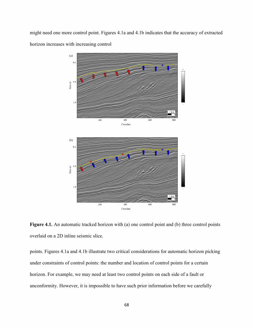
68

might need one more control point. Figures 4.1a and 4.1b indicates that the accuracy of extracted

horizon increases with increasing control

Figure 4.1. An automatic tracked horizon with (a) one control point and (b) three control points

overlaid on a 2D inline seismic slice.

points. Figures 4.1a and 4.1b illustrate two critical considerations for automatic horizon picking

under constraints of control points: the number and location of control points for a certain

horizon. For example, we may need at least two control points on each side of a fault or

unconformity. However, it is impossible to have such prior information before we carefully

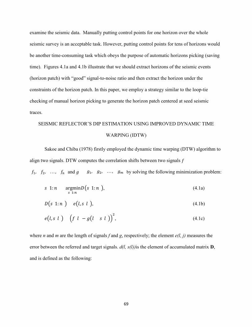
69

examine the seismic data. Manually putting control points for one horizon over the whole

seismic survey is an acceptable task. However, putting control points for tens of horizons would

be another time-consuming task which obeys the purpose of automatic horizons picking (saving

time). Figures 4.1a and 4.1b illustrate that we should extract horizons of the seismic events

(horizon patch) with “good” signal-to-noise ratio and then extract the horizon under the

constraints of the horizon patch. In this paper, we employ a strategy similar to the loop-tie

checking of manual horizon picking to generate the horizon patch centered at seed seismic

traces.

SEISMIC REFLECTOR’S DIP ESTIMATION USING IMPROVED DYNAMIC TIME

WARPING (IDTW)

Sakoe and Chiba (1978) firstly employed the dynamic time warping (DTW) algorithm to

align two signals. DTW computes the correlation shifts between two signals 𝑓𝑓 =

(𝑓𝑓1, 𝑓𝑓2, . . . , 𝑓𝑓𝑛𝑛) and 𝑔𝑔 = (𝑔𝑔1, 𝑔𝑔2, . . . , 𝑔𝑔𝑚𝑚) by solving the following minimization problem:

𝑠𝑠 (1:𝑛𝑛) = argmin𝑠𝑠 (1:𝑛𝑛)

𝐷𝐷 �𝑠𝑠(1:𝑛𝑛)�, (4.1a)

𝐷𝐷�𝑠𝑠(1:𝑛𝑛)� = 𝑒𝑒�𝑙𝑙, 𝑠𝑠(𝑙𝑙)�, (4.1b)

𝑒𝑒�𝑙𝑙, 𝑠𝑠(𝑙𝑙)� = �𝑓𝑓(𝑙𝑙) − 𝑔𝑔�𝑙𝑙 + 𝑠𝑠(𝑙𝑙)��2, (4.1c)

where n and m are the length of signals f and g, respectively; the element e(l, j) measures the

error between the referred and target signals. d(l, s(l))is the element of accumulated matrix D,

and is defined as the following:

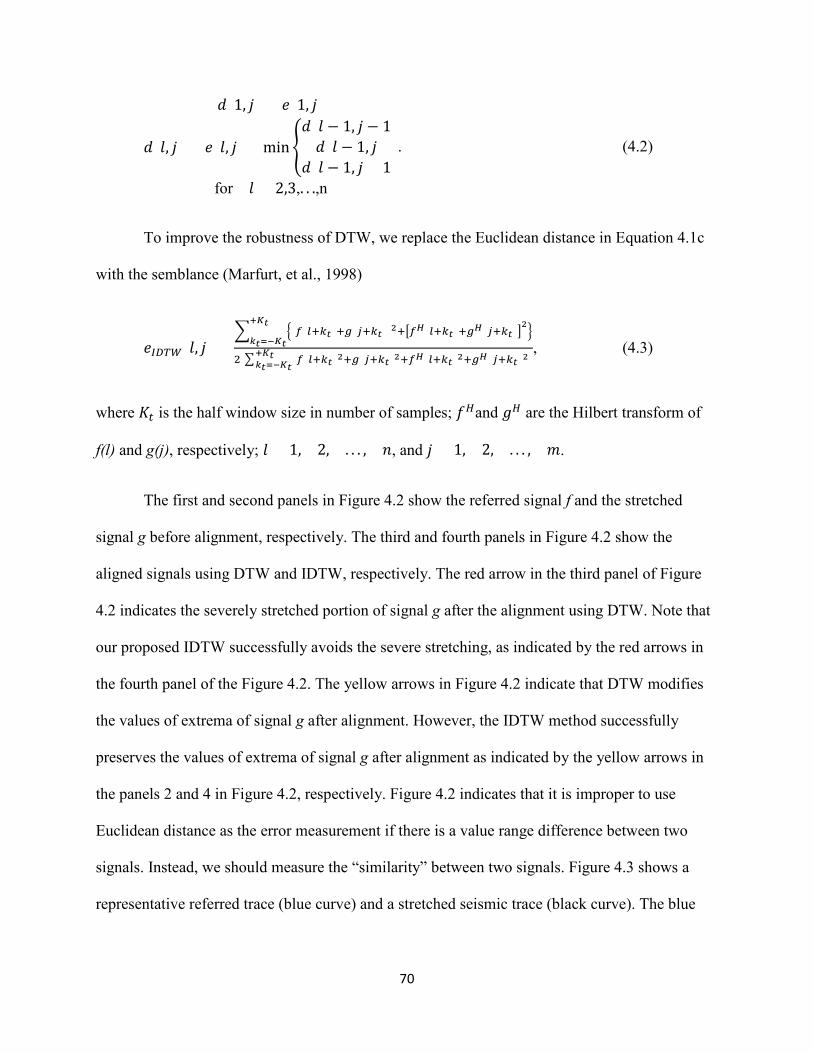
70

𝑑𝑑(1, 𝑗𝑗) = 𝑒𝑒(1, 𝑗𝑗)

𝑑𝑑(𝑙𝑙, 𝑗𝑗) = 𝑒𝑒(𝑙𝑙, 𝑗𝑗) + min�𝑑𝑑(𝑙𝑙 − 1, 𝑗𝑗 − 1)𝑑𝑑(𝑙𝑙 − 1, 𝑗𝑗)

𝑑𝑑(𝑙𝑙 − 1, 𝑗𝑗 + 1)for 𝑙𝑙 = 2,3,. . .,n

. (4.2)

To improve the robustness of DTW, we replace the Euclidean distance in Equation 4.1c

with the semblance (Marfurt, et al., 1998)

𝑒𝑒𝐼𝐼𝐼𝐼𝐼𝐼𝐼𝐼(𝑙𝑙, 𝑗𝑗) =� �[𝑓𝑓(𝑙𝑙+𝑘𝑘𝑡𝑡)+𝑔𝑔(𝑗𝑗+𝑘𝑘𝑡𝑡)]2+�𝑓𝑓𝐻𝐻(𝑙𝑙+𝑘𝑘𝑡𝑡)+𝑔𝑔𝐻𝐻(𝑗𝑗+𝑘𝑘𝑡𝑡)�

2�

+𝐾𝐾𝑡𝑡

𝑘𝑘𝑡𝑡=−𝐾𝐾𝑡𝑡

2� {𝑓𝑓(𝑙𝑙+𝑘𝑘𝑡𝑡)2+𝑔𝑔(𝑗𝑗+𝑘𝑘𝑡𝑡)2+𝑓𝑓𝐻𝐻(𝑙𝑙+𝑘𝑘𝑡𝑡)2+𝑔𝑔𝐻𝐻(𝑗𝑗+𝑘𝑘𝑡𝑡)2}+𝐾𝐾𝑡𝑡𝑘𝑘𝑡𝑡=−𝐾𝐾𝑡𝑡

, (4.3)

where 𝐾𝐾𝑡𝑡 is the half window size in number of samples; 𝑓𝑓𝐻𝐻and 𝑔𝑔𝐻𝐻 are the Hilbert transform of

f(l) and g(j), respectively; 𝑙𝑙 = 1, 2, . . . , 𝑛𝑛, and 𝑗𝑗 = 1, 2, . . . , 𝑚𝑚.

The first and second panels in Figure 4.2 show the referred signal f and the stretched

signal g before alignment, respectively. The third and fourth panels in Figure 4.2 show the

aligned signals using DTW and IDTW, respectively. The red arrow in the third panel of Figure

4.2 indicates the severely stretched portion of signal g after the alignment using DTW. Note that

our proposed IDTW successfully avoids the severe stretching, as indicated by the red arrows in

the fourth panel of the Figure 4.2. The yellow arrows in Figure 4.2 indicate that DTW modifies

the values of extrema of signal g after alignment. However, the IDTW method successfully

preserves the values of extrema of signal g after alignment as indicated by the yellow arrows in

the panels 2 and 4 in Figure 4.2, respectively. Figure 4.2 indicates that it is improper to use

Euclidean distance as the error measurement if there is a value range difference between two

signals. Instead, we should measure the “similarity” between two signals. Figure 4.3 shows a

representative referred trace (blue curve) and a stretched seismic trace (black curve). The blue

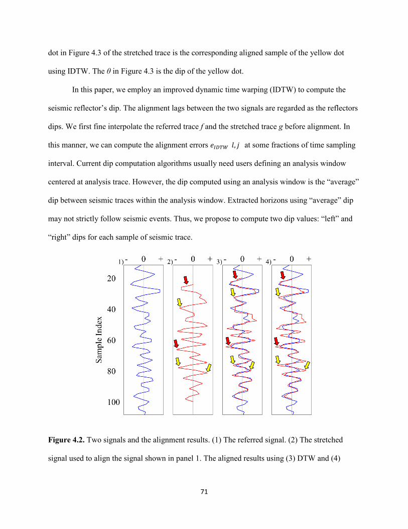
71

dot in Figure 4.3 of the stretched trace is the corresponding aligned sample of the yellow dot

using IDTW. The θ in Figure 4.3 is the dip of the yellow dot.

In this paper, we employ an improved dynamic time warping (IDTW) to compute the

seismic reflector’s dip. The alignment lags between the two signals are regarded as the reflectors

dips. We first fine interpolate the referred trace f and the stretched trace g before alignment. In

this manner, we can compute the alignment errors 𝑒𝑒𝐼𝐼𝐼𝐼𝐼𝐼𝐼𝐼(𝑙𝑙, 𝑗𝑗) at some fractions of time sampling

interval. Current dip computation algorithms usually need users defining an analysis window

centered at analysis trace. However, the dip computed using an analysis window is the “average”

dip between seismic traces within the analysis window. Extracted horizons using “average” dip

may not strictly follow seismic events. Thus, we propose to compute two dip values: “left” and

“right” dips for each sample of seismic trace.

Figure 4.2. Two signals and the alignment results. (1) The referred signal. (2) The stretched

signal used to align the signal shown in panel 1. The aligned results using (3) DTW and (4)

72

IDTW. The yellow and red arrows indicate modified signal values and severe stretching using

DTW, respectively.

Figure 4.3. The calculated reflector dip of the representative sample (yellow dot) using IDTW.

Panels 1 and 2 show the referred signal and the stretched signal, respectively.

LOOP-TIE CHECKING OF AUTOMATICALLY EXTRACTED HORIZON

Manual horizon picking is performed on inline and crossline vertical slices

independently. Thus, an important task is checking whether picked horizons of the same seismic

traces on inline and crossline vertical slices pass through the same two-way travel time and this

task is named as loop-tie. Although 3D automatic horizon extracting algorithms produce

horizons meeting the loop-tie checking. There is no guarantee that the extracted horizon strictly

follows the same seismic reflection event. Automatic horizon picking algorithms are based on

pre-computed seismic attributes such as seismic reflector’s dip. Considering that signal-to-noise

ratio of seismic events varies within the 3D seismic survey, it is impossible to obtain an accurate

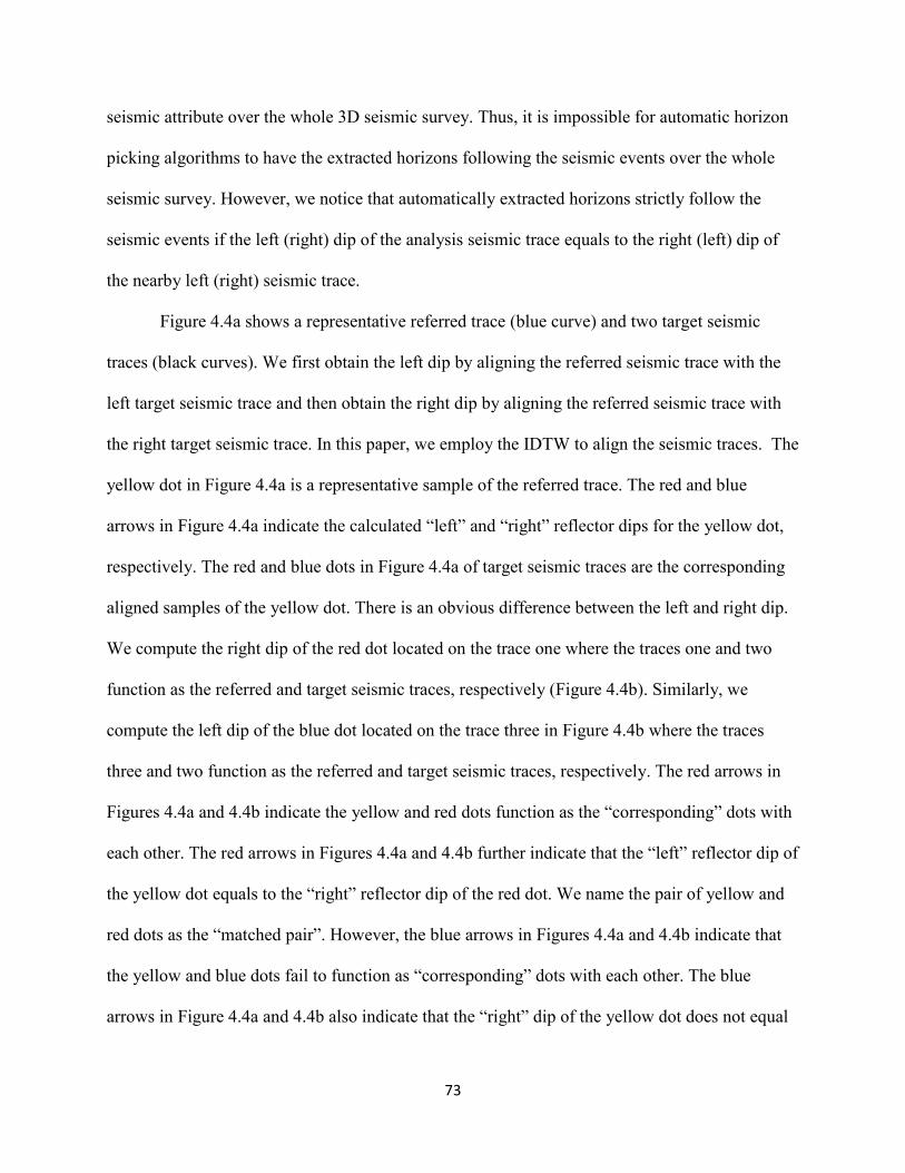
73

seismic attribute over the whole 3D seismic survey. Thus, it is impossible for automatic horizon

picking algorithms to have the extracted horizons following the seismic events over the whole

seismic survey. However, we notice that automatically extracted horizons strictly follow the

seismic events if the left (right) dip of the analysis seismic trace equals to the right (left) dip of

the nearby left (right) seismic trace.

Figure 4.4a shows a representative referred trace (blue curve) and two target seismic

traces (black curves). We first obtain the left dip by aligning the referred seismic trace with the

left target seismic trace and then obtain the right dip by aligning the referred seismic trace with

the right target seismic trace. In this paper, we employ the IDTW to align the seismic traces. The

yellow dot in Figure 4.4a is a representative sample of the referred trace. The red and blue

arrows in Figure 4.4a indicate the calculated “left” and “right” reflector dips for the yellow dot,

respectively. The red and blue dots in Figure 4.4a of target seismic traces are the corresponding

aligned samples of the yellow dot. There is an obvious difference between the left and right dip.

We compute the right dip of the red dot located on the trace one where the traces one and two

function as the referred and target seismic traces, respectively (Figure 4.4b). Similarly, we

compute the left dip of the blue dot located on the trace three in Figure 4.4b where the traces

three and two function as the referred and target seismic traces, respectively. The red arrows in

Figures 4.4a and 4.4b indicate the yellow and red dots function as the “corresponding” dots with

each other. The red arrows in Figures 4.4a and 4.4b further indicate that the “left” reflector dip of

the yellow dot equals to the “right” reflector dip of the red dot. We name the pair of yellow and

red dots as the “matched pair”. However, the blue arrows in Figures 4.4a and 4.4b indicate that

the yellow and blue dots fail to function as “corresponding” dots with each other. The blue

arrows in Figure 4.4a and 4.4b also indicate that the “right” dip of the yellow dot does not equal

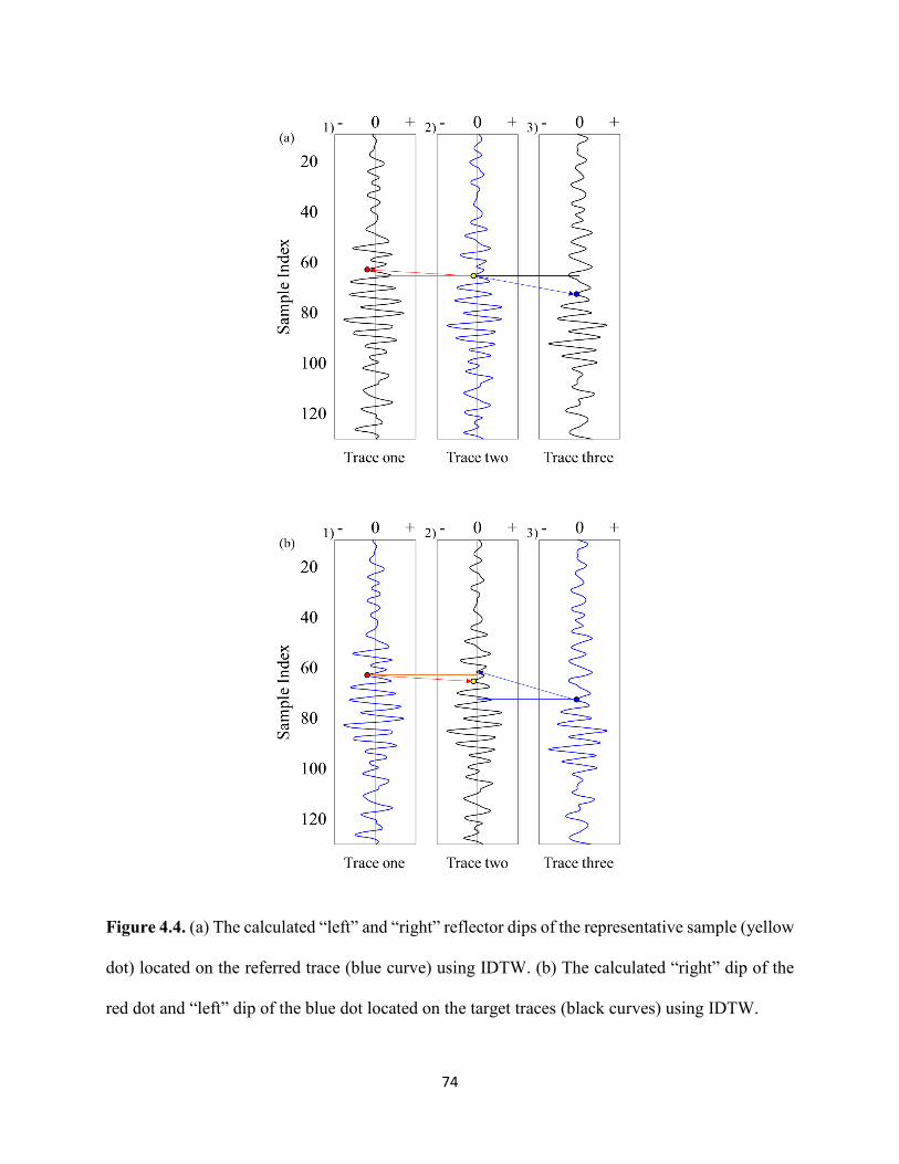
74

Figure 4.4. (a) The calculated “left” and “right” reflector dips of the representative sample (yellow

dot) located on the referred trace (blue curve) using IDTW. (b) The calculated “right” dip of the

red dot and “left” dip of the blue dot located on the target traces (black curves) using IDTW.

75

the “left” dip of the blue dot. We name the pair of yellow and blue dots as the “mismatched

pair”.

Our algorithm tracks the horizons on inline and crossline slices independently. We use

equation 4.4 to obtain the two-way travel time of trace j if trace j is located at the right side of the

referred seismic trace k

𝑡𝑡(𝑗𝑗) = 𝑡𝑡𝑠𝑠𝑠𝑠𝑠𝑠𝑠𝑠 + ∑ ∆𝑡𝑡𝑚𝑚𝑟𝑟𝑟𝑟𝑔𝑔ℎ𝑡𝑡�𝑡𝑡(𝑚𝑚)�𝑗𝑗−1

𝑘𝑘+1 , (4.4a)

𝑘𝑘 + 1 ≤ 𝑚𝑚 ≤ 𝑗𝑗 − 1, (4.4b)

where 𝑡𝑡𝑠𝑠𝑠𝑠𝑠𝑠𝑠𝑠 is the two-way travel time of the control point at the referred seismic trace k;

∆𝑡𝑡𝑚𝑚𝑟𝑟𝑟𝑟𝑔𝑔ℎ𝑡𝑡�𝑡𝑡(𝑚𝑚)� is the right dip of the trace m at two-way travel of 𝑡𝑡(𝑚𝑚). We use equation 4.5 to

obtain the two-way travel time of trace i if trace i is located at the left side of referred seismic

trace k

𝑡𝑡(𝑖𝑖) = 𝑡𝑡𝑠𝑠𝑠𝑠𝑠𝑠𝑠𝑠 − ∑ ∆𝑡𝑡𝑛𝑛𝑙𝑙𝑠𝑠𝑓𝑓𝑡𝑡�𝑡𝑡(𝑛𝑛)�𝑟𝑟−1

𝑘𝑘−1 , (4.5a)

𝑘𝑘 − 1 ≤ 𝑛𝑛 ≤ 𝑖𝑖 − 1. (4.5b)

Where ∆𝑡𝑡𝑛𝑛𝑙𝑙𝑠𝑠𝑓𝑓𝑡𝑡�𝑡𝑡(𝑛𝑛)� is the left dip of the trace n at two-way travel of t(n).

The loop tie checking of our algorithm is based on forward and backward horizon

tracking and consists of horizon tracking on inline and crossline slices independently. The

vertical yellow line in Figure 4.5a is the seed seismic trace and the blue cross mark indicates the

control point. We first use equations 4.4 and 4.5 to track the horizon, which is the yellow curve

in Figure 4.5a, on an inline vertical slice and this procedure is name as “forward horizon

tracking”. Then we treat the extracted two-way time, which are the pink cross marks in Figures

4.5a and 4.5b, of trace j (other than the seed seismic trace) as the control point. We use equation

76

4.4, if trace j is located at the left side of the seed trace, or equation 4.5, if trace j is located at the

right side of the seed trace, to generate a backward horizon. The back tracking is performed until

the initial control point is reached (blue cross marker in Figure 4.5a).

The red dash curves in Figures 4.5a and 4.5b show two representative backward tracked

horizons. The forward tracked horizon in Figure 4.5a (yellow curve) and the backward tracked

horizon (red dashed curve) perfectly coincides with each other, and the extracted horizon at trace

j in Figure 4.5a is a loop tie meeting extraction. The backward extracted horizon in Figure 4.5b

fails to coincide with each other and the extracted horizon at trace j in Figure 4.5b is not a loop

tie meeting extraction. Loop tie checking is performed for each seismic trace of the inline slice

and we only keep those extracted two-way travel time of seismic traces that are loop tie meeting

extractions. The accepted portion and rejected portion of the horizon are yellow and red curves

shown in Figure 4.5c, respectively.

Loop-tie checking is based on analyzing the relationship between extracted horizons on

nearby inline and crossline slices. Figure 4.6a demonstrates the steps of checking whether the

automatically extracted horizons between nearby inline and crossline slices meet the loop-tie.

Inline seismic slice AA’ and corresponding yellow curve in Figure 4.6a are the same seismic

slice and extracted yellow horizon shown in Figure 4.5a. The extracted horizon between seismic

trace number four and seismic trace number one is the same accepted yellow horizon shown in

Figure 4.5c. We then automatically track the horizon along crossline BB’ where seismic trace

number 1 is the referred seismic trace, and the extracted two-way travel time of trace number 1 is

the control point. We accept the extracted horizon between seismic traces number 1 and number

2 on crossline slice BB’ using the loop-tie checking procedure illustrated in Figure 4.5. We next

track the horizon along crossline slice DD’ where the seismic trace number 4 as referred seismic

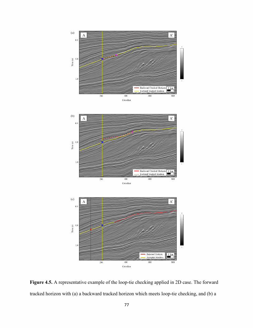
77

Figure 4.5. A representative example of the loop-tie checking applied in 2D case. The forward

tracked horizon with (a) a backward tracked horizon which meets loop-tie checking, and (b) a

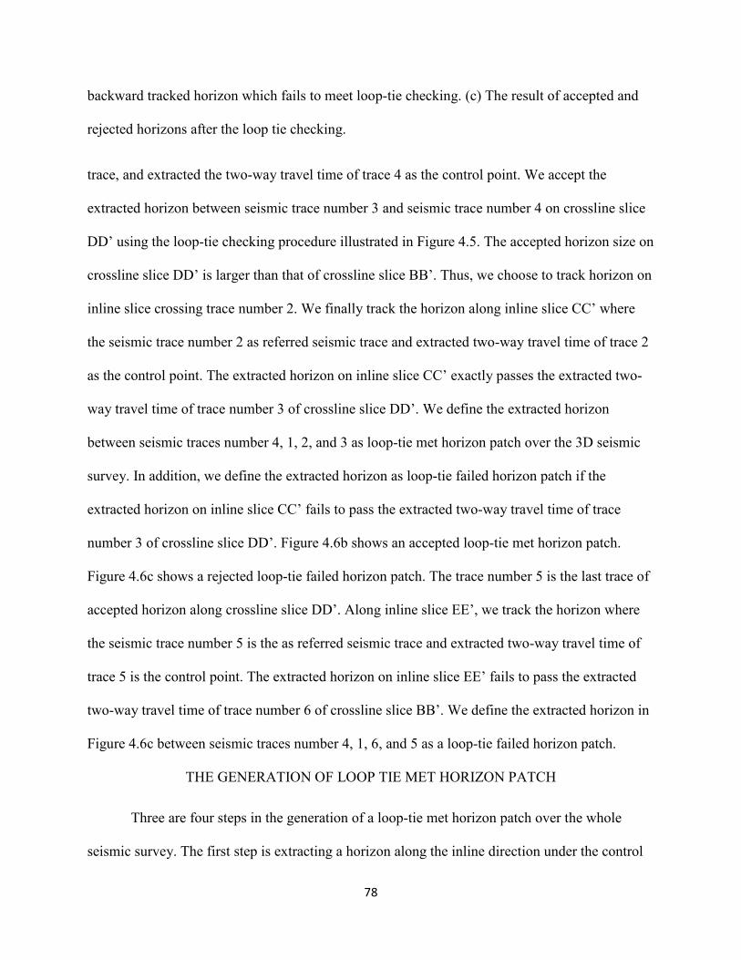
78

backward tracked horizon which fails to meet loop-tie checking. (c) The result of accepted and

rejected horizons after the loop tie checking.

trace, and extracted the two-way travel time of trace 4 as the control point. We accept the

extracted horizon between seismic trace number 3 and seismic trace number 4 on crossline slice

DD’ using the loop-tie checking procedure illustrated in Figure 4.5. The accepted horizon size on

crossline slice DD’ is larger than that of crossline slice BB’. Thus, we choose to track horizon on

inline slice crossing trace number 2. We finally track the horizon along inline slice CC’ where

the seismic trace number 2 as referred seismic trace and extracted two-way travel time of trace 2

as the control point. The extracted horizon on inline slice CC’ exactly passes the extracted two-

way travel time of trace number 3 of crossline slice DD’. We define the extracted horizon

between seismic traces number 4, 1, 2, and 3 as loop-tie met horizon patch over the 3D seismic

survey. In addition, we define the extracted horizon as loop-tie failed horizon patch if the

extracted horizon on inline slice CC’ fails to pass the extracted two-way travel time of trace

number 3 of crossline slice DD’. Figure 4.6b shows an accepted loop-tie met horizon patch.

Figure 4.6c shows a rejected loop-tie failed horizon patch. The trace number 5 is the last trace of

accepted horizon along crossline slice DD’. Along inline slice EE’, we track the horizon where

the seismic trace number 5 is the as referred seismic trace and extracted two-way travel time of

trace 5 is the control point. The extracted horizon on inline slice EE’ fails to pass the extracted

two-way travel time of trace number 6 of crossline slice BB’. We define the extracted horizon in

Figure 4.6c between seismic traces number 4, 1, 6, and 5 as a loop-tie failed horizon patch.

THE GENERATION OF LOOP TIE MET HORIZON PATCH

Three are four steps in the generation of a loop-tie met horizon patch over the whole

seismic survey. The first step is extracting a horizon along the inline direction under the control

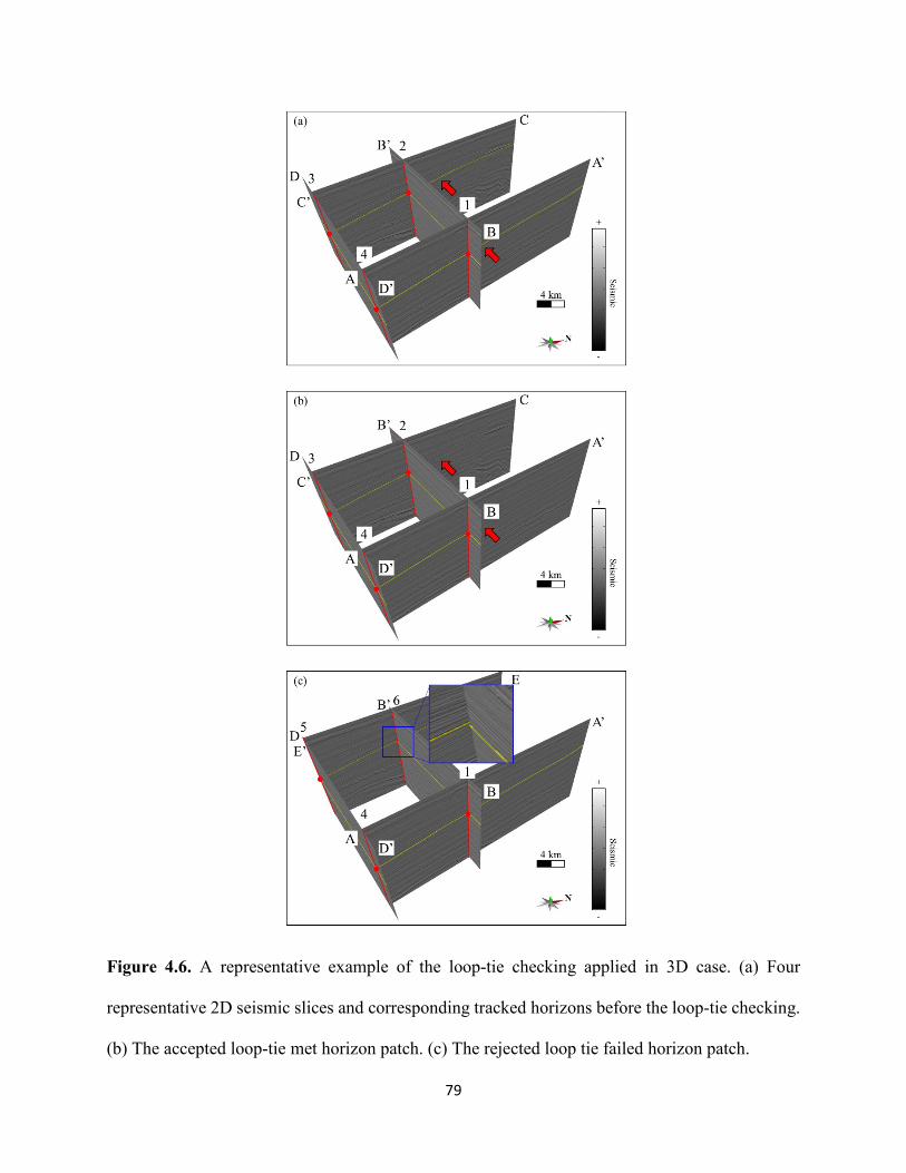
79

Figure 4.6. A representative example of the loop-tie checking applied in 3D case. (a) Four

representative 2D seismic slices and corresponding tracked horizons before the loop-tie checking.

(b) The accepted loop-tie met horizon patch. (c) The rejected loop tie failed horizon patch.

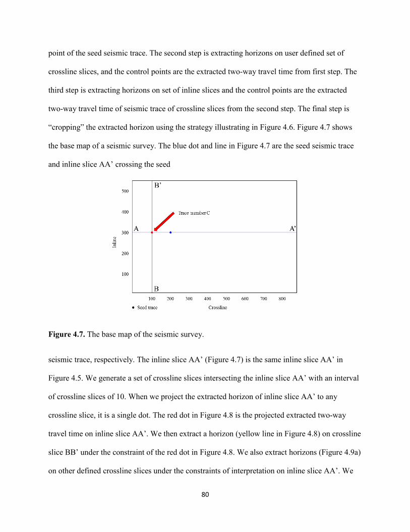
80

point of the seed seismic trace. The second step is extracting horizons on user defined set of

crossline slices, and the control points are the extracted two-way travel time from first step. The

third step is extracting horizons on set of inline slices and the control points are the extracted

two-way travel time of seismic trace of crossline slices from the second step. The final step is

“cropping” the extracted horizon using the strategy illustrating in Figure 4.6. Figure 4.7 shows

the base map of a seismic survey. The blue dot and line in Figure 4.7 are the seed seismic trace

and inline slice AA’ crossing the seed

Figure 4.7. The base map of the seismic survey.

seismic trace, respectively. The inline slice AA’ (Figure 4.7) is the same inline slice AA’ in

Figure 4.5. We generate a set of crossline slices intersecting the inline slice AA’ with an interval

of crossline slices of 10. When we project the extracted horizon of inline slice AA’ to any

crossline slice, it is a single dot. The red dot in Figure 4.8 is the projected extracted two-way

travel time on inline slice AA’. We then extract a horizon (yellow line in Figure 4.8) on crossline

slice BB’ under the constraint of the red dot in Figure 4.8. We also extract horizons (Figure 4.9a)

on other defined crossline slices under the constraints of interpretation on inline slice AA’. We

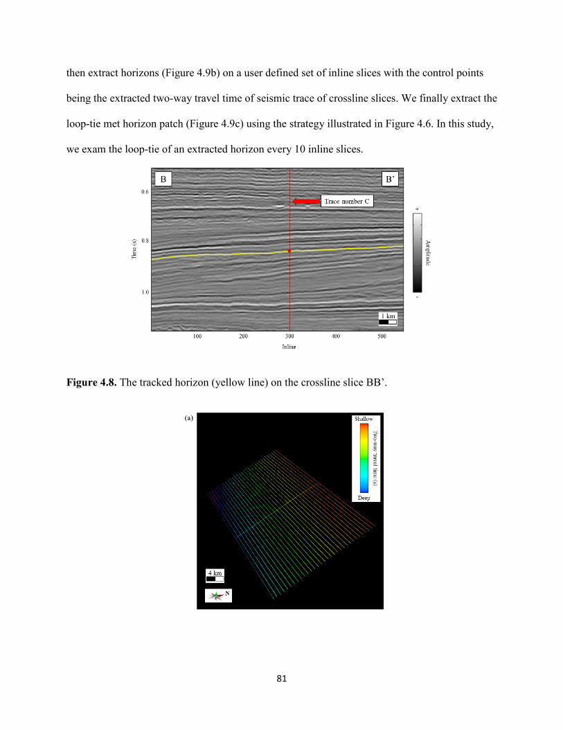
81

then extract horizons (Figure 4.9b) on a user defined set of inline slices with the control points

being the extracted two-way travel time of seismic trace of crossline slices. We finally extract the

loop-tie met horizon patch (Figure 4.9c) using the strategy illustrated in Figure 4.6. In this study,

we exam the loop-tie of an extracted horizon every 10 inline slices.

Figure 4.8. The tracked horizon (yellow line) on the crossline slice BB’.

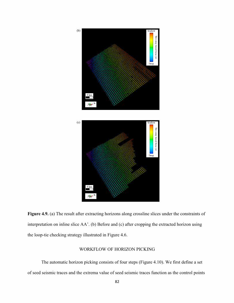
82

Figure 4.9. (a) The result after extracting horizons along crossline slices under the constraints of

interpretation on inline slice AA’. (b) Before and (c) after cropping the extracted horizon using

the loop-tie checking strategy illustrated in Figure 4.6.

WORKFLOW OF HORIZON PICKING

The automatic horizon picking consists of four steps (Figure 4.10). We first define a set

of seed seismic traces and the extrema value of seed seismic traces function as the control points

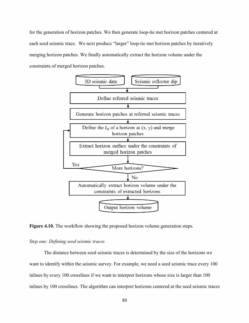
83

for the generation of horizon patches. We then generate loop-tie met horizon patches centered at

each seed seismic trace. We next produce “larger” loop-tie met horizon patches by iteratively

merging horizon patches. We finally automatically extract the horizon volume under the

constraints of merged horizon patches.

Figure 4.10. The workflow showing the proposed horizon volume generation steps.

Step one: Defining seed seismic traces

The distance between seed seismic traces is determined by the size of the horizons we

want to identify within the seismic survey. For example, we need a seed seismic trace every 100

inlines by every 100 crosslines if we want to interpret horizons whose size is larger than 100

inlines by 100 crosslines. The algorithm can interpret horizons centered at the seed seismic traces

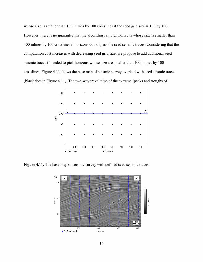
84

whose size is smaller than 100 inlines by 100 crosslines if the seed grid size is 100 by 100.

However, there is no guarantee that the algorithm can pick horizons whose size is smaller than

100 inlines by 100 crosslines if horizons do not pass the seed seismic traces. Considering that the

computation cost increases with decreasing seed grid size, we propose to add additional seed

seismic traces if needed to pick horizons whose size are smaller than 100 inlines by 100

crosslines. Figure 4.11 shows the base map of seismic survey overlaid with seed seismic traces

(black dots in Figure 4.11). The two-way travel time of the extrema (peaks and troughs of

Figure 4.11. The base map of seismic survey with defined seed seismic traces.

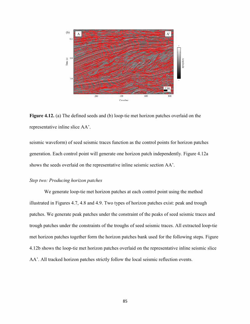
85

Figure 4.12. (a) The defined seeds and (b) loop-tie met horizon patches overlaid on the

representative inline slice AA’.

seismic waveform) of seed seismic traces function as the control points for horizon patches

generation. Each control point will generate one horizon patch independently. Figure 4.12a

shows the seeds overlaid on the representative inline seismic section AA’.

Step two: Producing horizon patches

We generate loop-tie met horizon patches at each control point using the method

illustrated in Figures 4.7, 4.8 and 4.9. Two types of horizon patches exist: peak and trough

patches. We generate peak patches under the constraint of the peaks of seed seismic traces and

trough patches under the constraints of the troughs of seed seismic traces. All extracted loop-tie

met horizon patches together form the horizon patches bank used for the following steps. Figure

4.12b shows the loop-tie met horizon patches overlaid on the representative inline seismic slice

AA’. All tracked horizon patches strictly follow the local seismic reflection events.

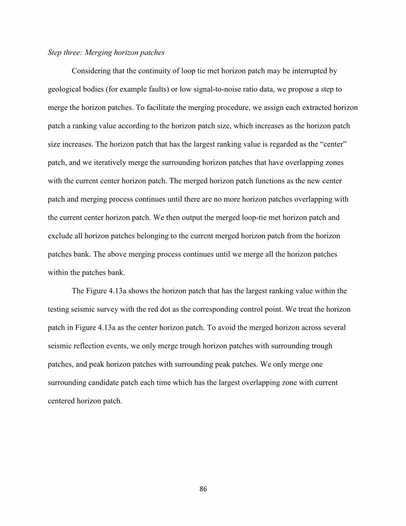
86

Step three: Merging horizon patches

Considering that the continuity of loop tie met horizon patch may be interrupted by

geological bodies (for example faults) or low signal-to-noise ratio data, we propose a step to

merge the horizon patches. To facilitate the merging procedure, we assign each extracted horizon

patch a ranking value according to the horizon patch size, which increases as the horizon patch

size increases. The horizon patch that has the largest ranking value is regarded as the “center”

patch, and we iteratively merge the surrounding horizon patches that have overlapping zones

with the current center horizon patch. The merged horizon patch functions as the new center

patch and merging process continues until there are no more horizon patches overlapping with

the current center horizon patch. We then output the merged loop-tie met horizon patch and

exclude all horizon patches belonging to the current merged horizon patch from the horizon

patches bank. The above merging process continues until we merge all the horizon patches

within the patches bank.

The Figure 4.13a shows the horizon patch that has the largest ranking value within the

testing seismic survey with the red dot as the corresponding control point. We treat the horizon

patch in Figure 4.13a as the center horizon patch. To avoid the merged horizon across several

seismic reflection events, we only merge trough horizon patches with surrounding trough

patches, and peak horizon patches with surrounding peak patches. We only merge one

surrounding candidate patch each time which has the largest overlapping zone with current

centered horizon patch.

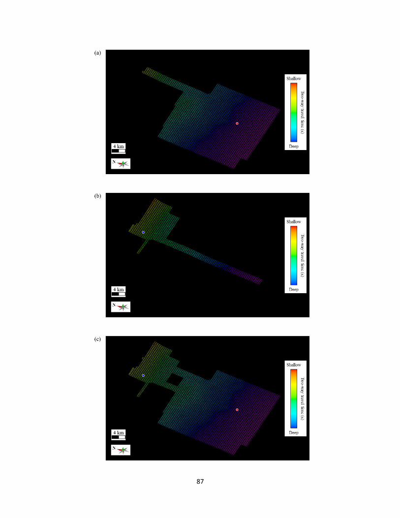
87

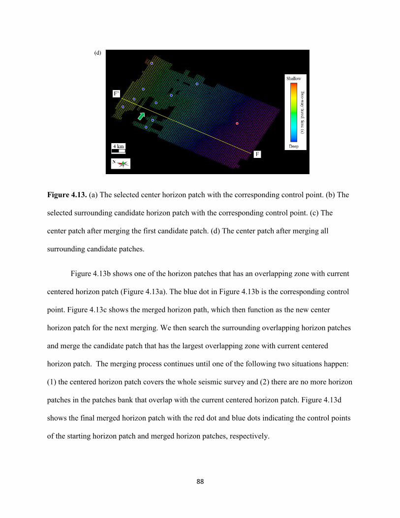
88

Figure 4.13. (a) The selected center horizon patch with the corresponding control point. (b) The

selected surrounding candidate horizon patch with the corresponding control point. (c) The

center patch after merging the first candidate patch. (d) The center patch after merging all

surrounding candidate patches.

Figure 4.13b shows one of the horizon patches that has an overlapping zone with current

centered horizon patch (Figure 4.13a). The blue dot in Figure 4.13b is the corresponding control

point. Figure 4.13c shows the merged horizon path, which then function as the new center

horizon patch for the next merging. We then search the surrounding overlapping horizon patches

and merge the candidate patch that has the largest overlapping zone with current centered

horizon patch. The merging process continues until one of the following two situations happen:

(1) the centered horizon patch covers the whole seismic survey and (2) there are no more horizon

patches in the patches bank that overlap with the current centered horizon patch. Figure 4.13d

shows the final merged horizon patch with the red dot and blue dots indicating the control points

of the starting horizon patch and merged horizon patches, respectively.

89

Considering that the accuracy of the extracted horizon increasing with number of control

points, our merging workflow also allows the manual merging of a horizon patch that does not

have an overlapping zone with current centered horizon patch. The green arrow in Figure 4.13d

indicates a relative large “empty” zone where there are no overlapping horizon patches with the

current merged centered horizon patch. The yellow line FF’ in Figure 4.13d is one inline slice

(Figure 4.14) crossing the empty zone. The yellow curve in Figure 4.14 is the merged centered

horizon patch. The red curve in Figure 4.14 locates at the same seismic reflection event tracked

by the yellow curve. Thus, we manually merge the horizon patch (indicated by the green arrow

in Figure 4.15a) that includes the red curve in Figure 4.14. The white dot in Figure 4.15a is the

control point generating the horizon patch indicated by the green arrow in Figure 4.15a. We

finally automatically extract the horizon (Figure 4.15b) over the whole seismic survey using the

seismic dip attribute with the merged horizon patch (Figure 4.15a) functioning as the control

point.

Figure 4.14. The merged horizon patch in Figure 13d overlaid on the representative inline

seismic slice FF’.

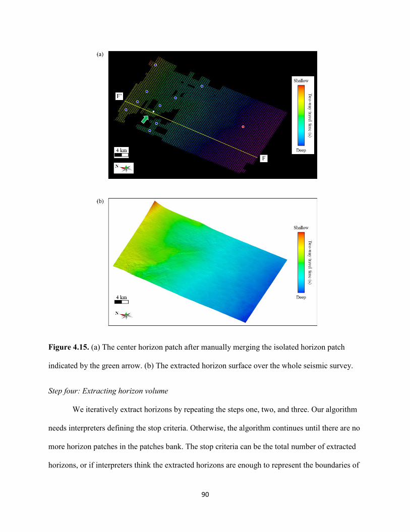
90

Figure 4.15. (a) The center horizon patch after manually merging the isolated horizon patch

indicated by the green arrow. (b) The extracted horizon surface over the whole seismic survey.

Step four: Extracting horizon volume

We iteratively extract horizons by repeating the steps one, two, and three. Our algorithm

needs interpreters defining the stop criteria. Otherwise, the algorithm continues until there are no

more horizon patches in the patches bank. The stop criteria can be the total number of extracted

horizons, or if interpreters think the extracted horizons are enough to represent the boundaries of

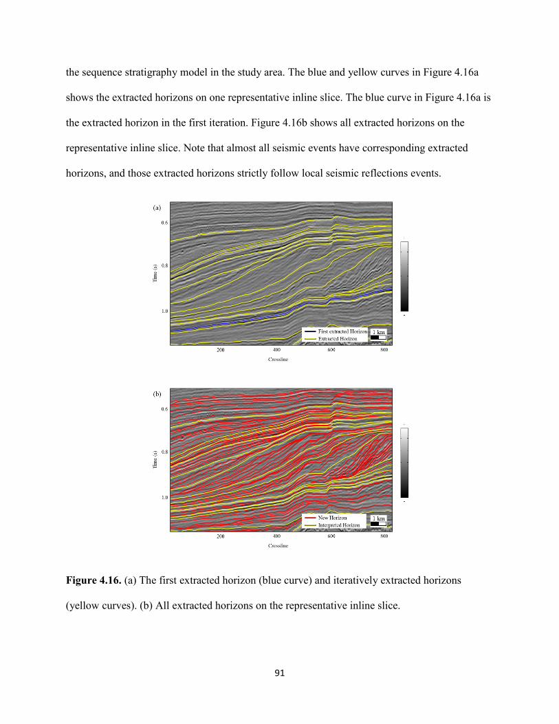
91

the sequence stratigraphy model in the study area. The blue and yellow curves in Figure 4.16a

shows the extracted horizons on one representative inline slice. The blue curve in Figure 4.16a is

the extracted horizon in the first iteration. Figure 4.16b shows all extracted horizons on the

representative inline slice. Note that almost all seismic events have corresponding extracted

horizons, and those extracted horizons strictly follow local seismic reflections events.

Figure 4.16. (a) The first extracted horizon (blue curve) and iteratively extracted horizons

(yellow curves). (b) All extracted horizons on the representative inline slice.

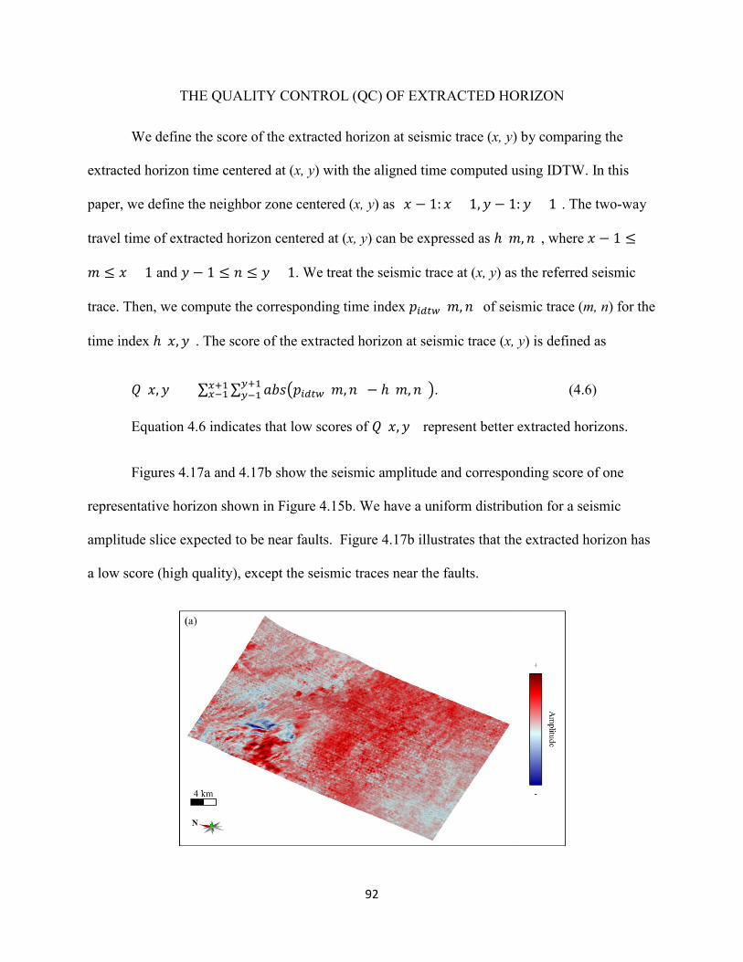
92

THE QUALITY CONTROL (QC) OF EXTRACTED HORIZON

We define the score of the extracted horizon at seismic trace (x, y) by comparing the

extracted horizon time centered at (x, y) with the aligned time computed using IDTW. In this

paper, we define the neighbor zone centered (x, y) as [𝑥𝑥 − 1: 𝑥𝑥 + 1,𝑦𝑦 − 1:𝑦𝑦 + 1]. The two-way

travel time of extracted horizon centered at (x, y) can be expressed as ℎ(𝑚𝑚,𝑛𝑛), where 𝑥𝑥 − 1 ≤

𝑚𝑚 ≤ 𝑥𝑥 + 1 and 𝑦𝑦 − 1 ≤ 𝑛𝑛 ≤ 𝑦𝑦 + 1. We treat the seismic trace at (x, y) as the referred seismic

trace. Then, we compute the corresponding time index 𝑝𝑝𝑟𝑟𝑠𝑠𝑡𝑡𝑖𝑖(𝑚𝑚,𝑛𝑛) of seismic trace (m, n) for the

time index ℎ(𝑥𝑥,𝑦𝑦). The score of the extracted horizon at seismic trace (x, y) is defined as

𝑄𝑄(𝑥𝑥,𝑦𝑦 ) = ∑ ∑ 𝑎𝑎𝑎𝑎𝑠𝑠�𝑝𝑝𝑟𝑟𝑠𝑠𝑡𝑡𝑖𝑖(𝑚𝑚,𝑛𝑛) − ℎ(𝑚𝑚,𝑛𝑛)�𝑦𝑦+1𝑦𝑦−1

𝑥𝑥+1𝑥𝑥−1 . (4.6)

Equation 4.6 indicates that low scores of 𝑄𝑄(𝑥𝑥,𝑦𝑦 ) represent better extracted horizons.

Figures 4.17a and 4.17b show the seismic amplitude and corresponding score of one

representative horizon shown in Figure 4.15b. We have a uniform distribution for a seismic

amplitude slice expected to be near faults. Figure 4.17b illustrates that the extracted horizon has

a low score (high quality), except the seismic traces near the faults.

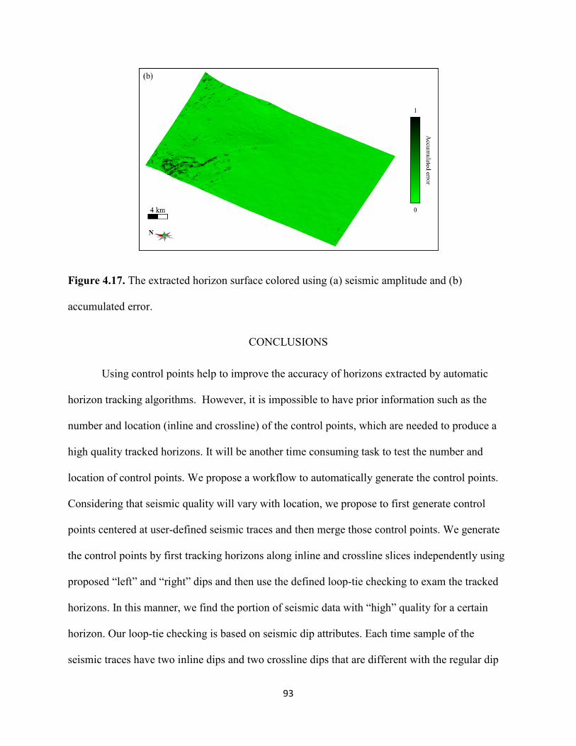
93

Figure 4.17. The extracted horizon surface colored using (a) seismic amplitude and (b)

accumulated error.

CONCLUSIONS

Using control points help to improve the accuracy of horizons extracted by automatic

horizon tracking algorithms. However, it is impossible to have prior information such as the

number and location (inline and crossline) of the control points, which are needed to produce a

high quality tracked horizons. It will be another time consuming task to test the number and

location of control points. We propose a workflow to automatically generate the control points.

Considering that seismic quality will vary with location, we propose to first generate control

points centered at user-defined seismic traces and then merge those control points. We generate

the control points by first tracking horizons along inline and crossline slices independently using

proposed “left” and “right” dips and then use the defined loop-tie checking to exam the tracked

horizons. In this manner, we find the portion of seismic data with “high” quality for a certain

horizon. Our loop-tie checking is based on seismic dip attributes. Each time sample of the

seismic traces have two inline dips and two crossline dips that are different with the regular dip

94

attributes. The four dip attribute values are used to ensure the generated control points have the

same accuracy of manual interpretation. Thus, those control points can function as the “hard”

constraints for the automatic horizon picking algorithms. The application demonstrates that the

extracted horizons using our proposed method exactly follow the local seismic reflection events.

95

REFERENCES

Bahorich, M., and S. Farmer, 1995, 3D seismic discontinuity for faults and stratigraphic features: The coherence cube: The Leading Edge, 14(10), 1053-1058.

Bakker, P., L. J. van Vliet, and P. W. Verbeek, 1999, Edge-preserving orientation adaptive filtering: IEEE Computer Society Conference on Computer Vision and Pattern Recognition, 1, 535-540.

Barnes, A. E., 1996, Theory of 2-D complex seismic trace analysis: Geophysics, 61(1), 264-272.

Borgos, H. G., T. Skov, T. Randen, and L. Sonneland, 2003, Automated geometry extraction from 3D seismic data: SEG Technical Program Expanded Abstracts 2003, 1541-1544.

Fehmers, G. C., and C. F. Höcker, 2003, Fast structural interpretation with structure-oriented filtering: Geophysics, 68(4), 1286-1293.

Fomel, S., 2010, Predictive painting of 3D seismic volumes: Geophysics, 75(4), A25–A30.

Lomask, J., A. Guitton, S. Fomel, J. Claerbout, and A. A. Valenciano, 2006, Flattening without picking: Geophysics, 71(4), P13-P20.

Lou, Y., B. Zhang, T. Lin, and D. Cao, 2019a, Automatic horizon picking using multiple seismic attributes: Geophysics, 85(2), 1-48.

Lou, Y., B. Zhang, T. Lin, N. Liu, H. Wu, R. Liu, and D. Cao, 2019b, Accurate seismic dip and azimuth estimation using multi-window scanning of structure-tensor: Geophysics, 84(5), 1-54.

Luo, Y., W. G. Higgs, and W. S. Kowalik, 1996, Edge detection and stratigraphic analysis using 3D seismic data: SEG Technical Program Expanded Abstracts 1996, 324-327.

Monsen, E. M., H. G. Borgos, P. L. Guern, and L. Sonneland, 2007, Geological process controlled interpretation based on 3D Wheeler diagram generation: SEG Technical Program Expanded Abstracts 2007, 885-889.

Marfurt, K. J., 2006, Robust estimates of 3D reflector dip and azimuth: Geophysics, 71(4), P29-P40.

Marfurt, K. J., R. L. Kirlin, S. L. Farmer, and M. S. Bahorich, 1998, 3-D seismic attributes using a semblance-based coherency algorithm: Geophysics, 63(4), 1150-1165.

Parks, D., 2010, Seismic image flattening as a linear inverse problem: Master’s thesis, Colorado School of Mines.

Sakoe, H., and S. Chiba, 1978, Dynamic programming algorithm optimization for spoken word recognition: IEEE Transactions on Acoustics, Speech, and Signal Processing, 26, 43–49.

96

Stark, T. J., 2004, Relative geologic time (age) volumes-Relating every seismic sample to a geologically reasonable horizon: The Leading Edge, 23(9), 928-932.

Wu, H., B. Zhang, T. Lin, D. Cao, and Y. Lou, 2019, Semi-automated seismic horizon interpretation using encoder-decoder convolutional neural network: Geophysics, 84(6), B403-B417.

Wu, X., and D. Hale, 2015, Horizon volumes with interpreted constraints: Geophysics, 80(2), IM21-IM33.

Wu, X., and G. Zhong, 2012, Generating a relative geologic time volume by 3D graph-cut phase unwarping method with horizon and unconformity constraints: Geophysics, 77(4), O21–O34.

Wu, X., and S. Fomel, 2018, Least-squares horizons with local slopes and multi-grid correlations, Geophysics, 83(4), IM29–IM40.

Wu, X. and X., Janson, 2017, Directional structure tensors in estimating seismic structural and stratigraphic orientations: Geophysical Journal International, 210(1), 534-548.

Zeng, H., M. M. Backus, K. T. Barrow, and N. Tyler, 1998, Stratal slicing, part I: realistic 3-D seismic model: Geophysics, 63(2), 502-513.

Zhang, B., Y. Lou, and H. Wu, 2019, Orientation estimate of 3D seismic events using dynamic programming: SEG Technical Program Expanded Abstracts 2019, 1873-1877.

Zinck, G., M. Donias, J. Daniel, S. Guillon, and O. Lavialle, 2013, Fast seismic horizon reconstruction based on local dip transformation: Journal of Applied Geophysics, 96, 11–18

97

CHAPTER 5 SEISMIC FAULT ATTRIBUTE ESTIMATION USING LOCAL FAULT MODEL

Yihuai Lou1, Bo Zhang1, Ruiqi Wang2, Tengfei Lin3 and Danping Cao4 1The University of Alabama, Department of Geological Science.

2Pennsylvania State University, Department of Energy and Mineral Engineering. 3Department of Middle East E&P, Research Institute of Petroleum Exploration & Development,

CNPC. 4China University of Petroleum (East China), School of Geoscience.

This paper was published by SEG journal Geophysics in 2019

ABSTRACT

Faults in the subsurface can be an avenue of, or a barrier to, hydrocarbon flow and

pressure communication. Manual interpretation of discontinuities on 3D seismic amplitude

volume is the most common way to define faults within a reservoir. Unfortunately, 3D seismic

fault interpretation can be a time-consuming and tedious task. Seismic attributes such as

coherence help define faults, but suffer from “staircase” artifacts and non-fault related

stratigraphic discontinuities. We assume that each sample of the seismic data is located at a

potential fault plane. The hypothesized fault divides the seismic data centered at the analysis

sample into two sub-windows. We then compute the coherence for the two sub-windows, and for

the full analysis window. We repeat the process by rotating the hypothesized fault plane along a

set of user-defined discrete fault dip and azimuth. We obtain almost same coherence values for

the sub-windows and full window if the analysis point is not located at a fault plane. The “best”

fault plane results in maximum coherence for the sub-windows and minimum coherence for the

full window if the analysis point is located at a fault plane. To improve the continuity of the fault

attributes, we finally smooth the fault probability attribute along the estimated fault plane. We

illustrate the effectiveness of our workflow by applying it to a synthetic and two real seismic

98

data. The results indicate the proposed workflow successfully produces continuous fault attribute

without staircase artifacts and stratigraphic discontinuities.

INTRODUCTION

Identification and mapping of faults is the first step in seismic structure interpretation in

both conventional and unconventional plays. The identification of major and subtle faults is

critical to identify potential drilling hazards, and understand the orientation and intensity of

potential natural fractures. For large datasets, handpicking faults is time-consuming, such that

any means to accelerate the process is attractive. Major faults are easily seen and picked by

experienced interpreters in areas of the seismic volume exhibiting a relatively good signal-to-

noise ratio; however, in other areas, more subtle faults are masked by noise. Twenty years after

the introduction of coherence, developing an accurate and sensitive fault attribute remains an

ongoing challenge.

Coherence measurements that detect structural discontinuities are normally used to assist

fault interpretation in 3D seismic survey. Fault detection algorithms fall into two categories. The

first category selects the sampling window without considering volumetric dip and azimuth.

Barnes (1996) and Luo et al. (1996) use complex trace analysis to detect faults and stratigraphic

boundaries in 3D seismic data. The gradient structure tensor (GST) is proposed to detect

discontinuities by utilizing the eigenvector that corresponds to the largest eigenvalue (Bakker et

al., 1999; Fehmers and Hoecker, 2003). Wu (2017) improves the fault detection performance of

GST based coherence by using the directional structure tensors. The second category employs

the volumetric dip and azimuth to compute coherence. The cross-correlation shifts traces by an

assumed dip (Bahorich and Farmer, 1995). Marfurt et al. (1998) generate the coherence

algorithm by computing semblance in a suite of windows aligned with candidate reflector dips.

99

Marfurt et al. (1999) generate the coherence algorithm by using the Eigenstructure of seismic

traces along the reflectors dip. The semblance-based coherence is further improved by

employing a multiple window Kuwahara filtering (Marfurt, 2006). Luo et al. (2002) and Wang et

al. (2008) use seismic volumetric dip and azimuth to detect sharp edges by using edge-preserving

smoothing. Donias et al. (2007) detect and isolate faults from noise by using the steered data-

analysis window over a set of dip and azimuth directions. Qi et al. (2017) propose a new way to

compute the energy-ratio coherence for azimuthally limited comprehensive data volumes. Some

other researchers (Neff et al., 2000; Cohen et al., 2006; Hale, 2009; Wu and Zhu, 2017) suggest

smoothing along fault strikes and dips to enhance fault features by scanning over all possible

combinations of fault strikes and dips. Similarly, Hale (2013) and Wu and Hale (2016) scan over

all possible fault orientations to compute fault likelihood or fault-oriented semblance. Other

methods, such as gradient magnitude (Aqrawi and Boe, 2011), and geosteering phase attributes

(Yuan et al., 2018; Wang et al., 2018), have been proposed to detect structural discontinuities.

Several researchers have proposed methods to improve the quality of coherence

attributes. Pedersen et al. (2002, 2003) proposed to enhance fault features along paths of

“artificial ants” by assuming the paths follow faults. Qi and Castagna (2013) detected the faults

of Barnett shale by applying principal component analysis to the seismic attributes. Zhang et al.

(2014) improved the coherence attributes by using a vein pattern recognition algorithm. Qi et al.

(2017, 2018) built a workflow to enhance and skeletonize coherence fault images along fault

planes. Wu and Fomel (2018) proposed an efficient method to extract optimal surfaces following

maximum fault attributes and use these optimal surfaces to vote for enhanced fault images of

fault probabilities, strikes and dips.

100

All coherence algorithms are computed using an oblique window centered at each

analysis voxel consisting of user-defined traces (horizontal) and time samples (vertical). Since

the size of the analysis window is oriented vertically along traces, the staircase artifacts are

caused by the vertical extent of the analysis window, where larger vertical extent results in

larger, smoother staircase artifacts (Marfurt and Lin, 2017). A remedy is to limit the vertical

analysis window to approximately the dominant period of the seismic data, thereby avoiding

mixing discontinuities from deeper or shallower horizons (Marfurt and Lin, 2017). However, it is

difficult to determine the window size which approximately equals to the local dominant period

of the seismic data. In this paper, we develop a new method to minimize the staircase artifacts

and undesired stratigraphic anomalies using a local fault model. Our method belongs to the

second category of fault detection algorithms. We assume that there exists a fault plane passing

through each voxel of our seismic data. The fault plane subdivides the original oblique analysis

window into two sub-windows. We determine the fault dip and azimuth by analyzing the

computed coherence of the two sub-windows. Then, we smooth the fault probability along the

local orientation of fault plane to minimize staircase artifacts and undesired stratigraphic

anomalies. We begin with illustrating how to compute the new fault attributes by using a local

fault model. We then demonstrate the effectiveness of our workflow by applying it to a synthetic

data and two real seismic data acquired over the offshore Netherlands (F3) and the marine New

Zealand (Kerry 3D), respectively.

METHOD

To minimize the effect of staircase artifacts and undesired stratigraphic discontinuities on

fault analysis in the seismic image, we propose a method (Figure 5.1) to generate the fault

attribute using a local fault model. Our method assumes that we have a local fault plane passing

101

through each analysis point. We obtain the dip and azimuth of the fault plane by rotating the fault

plane along a set of discrete dip and azimuth. We obtain the fault probability at the analysis

window by statistically evaluating the computed coherence for each candidate fault.

Figure 5.1. Workflow for the new fault attribute based on a local fault model.

Coherence computation using a local fault model

Our method begins by defining a set of assumed fault planes centered at the analysis

point. We generate the assumed fault planes by defining the minimum, maximum, and increment

of the fault scanning dip and azimuth. The yellow stars and yellow lines in Figures 5.2a, 5.2b,

and 4.2c denote the analysis points and three candidate faults, respectively. The dip angles in

102

Figures 5.2a, 5.2b, 5.2c are 90o, 45o, and the dip angle coincident with the fault plane,

respectively. The assumed faults (yellow lines in Figure 5.2a, 5.2b, and 5.2c) divide the 2D

analysis window into two sub-windows. The left and right sub-windows is composed of red and

blue seismic data, respectively. The yellow surface in Figure 5.3 shows a representative assumed

fault plane in 3D. The red and blue traces in Figure 5.3 form two separate sub-analysis windows.

We then compute the semblance-based coherence S for each sub-window by considering

the local reflector’s dip (Marfurt et al., 1998).

( ) ( )

( )[ ] ( )[ ]∑ ∑

∑ ∑∑+

−= =

+

−= ==

−−++−−+

−−++

−−+

=t

tt

t

tt

M

Mm

N

1n

2nnnnt0

H2nnnnt0

M

Mm

2N

1nnnnnt0

H2N

1nnnnnt0

y,x,qypxmτfy,x,qypxmτfN

y,x,qypxmτfy,x,qypxmτf

S, (5.1)

where Hf is the Hilbert transform of the real seismic trace, f ; t is the two-way travel time; x

and y are the inline and crossline coordinates, respectively; Mt is the half window size in number

of samples; N is the number of seismic traces in the analysis window; τ0 is the time of the center

analysis point; p and q are the reflector dips in the inline and crossline directions, respectively.

The coherence value of the seismic data within the left and right sub-windows are named

as Cleft and Cright, respectively. We also use equation 5.1 to compute the coherence Cfull for the

full analysis window, where the full analysis window includes the seismic data in both the left

(red) and right (blue) sub-windows. Note that we obtain the most coherent seismic traces for the

left and right sub-windows if the assumed fault plane is coincident with the true fault plane. We

should obtain the lowest value of Cfull if the assumed fault plane is parallel the true fault plane. If

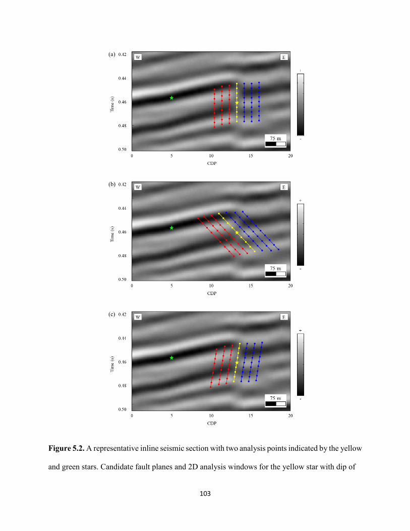
103

Figure 5.2. A representative inline seismic section with two analysis points indicated by the yellow

and green stars. Candidate fault planes and 2D analysis windows for the yellow star with dip of

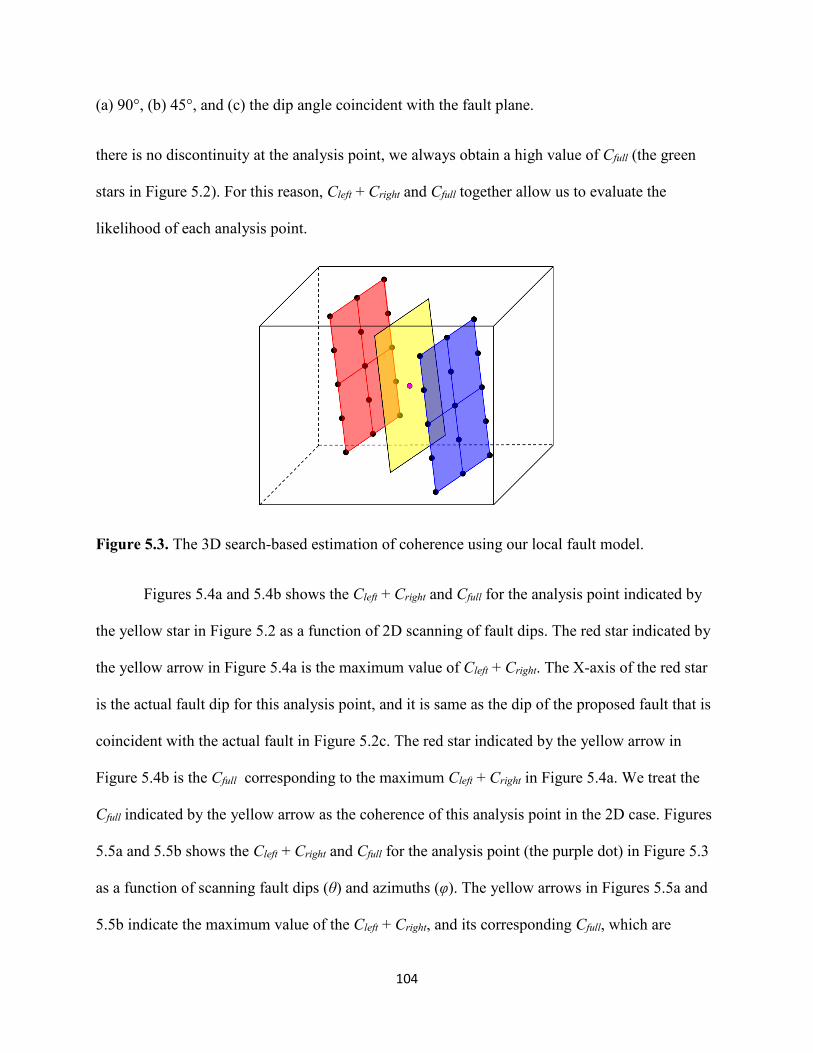
104

(a) 90°, (b) 45°, and (c) the dip angle coincident with the fault plane.

there is no discontinuity at the analysis point, we always obtain a high value of Cfull (the green

stars in Figure 5.2). For this reason, Cleft + Cright and Cfull together allow us to evaluate the

likelihood of each analysis point.

Figure 5.3. The 3D search-based estimation of coherence using our local fault model.

Figures 5.4a and 5.4b shows the Cleft + Cright and Cfull for the analysis point indicated by

the yellow star in Figure 5.2 as a function of 2D scanning of fault dips. The red star indicated by

the yellow arrow in Figure 5.4a is the maximum value of Cleft + Cright. The X-axis of the red star

is the actual fault dip for this analysis point, and it is same as the dip of the proposed fault that is

coincident with the actual fault in Figure 5.2c. The red star indicated by the yellow arrow in

Figure 5.4b is the Cfull corresponding to the maximum Cleft + Cright in Figure 5.4a. We treat the

Cfull indicated by the yellow arrow as the coherence of this analysis point in the 2D case. Figures

5.5a and 5.5b shows the Cleft + Cright and Cfull for the analysis point (the purple dot) in Figure 5.3

as a function of scanning fault dips (θ) and azimuths (φ). The yellow arrows in Figures 5.5a and

5.5b indicate the maximum value of the Cleft + Cright, and its corresponding Cfull, which are

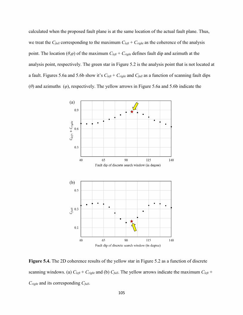
105

calculated when the proposed fault plane is at the same location of the actual fault plane. Thus,

we treat the Cfull corresponding to the maximum Cleft + Cright as the coherence of the analysis

point. The location (θ,φ) of the maximum Cleft + Cright defines fault dip and azimuth at the

analysis point, respectively. The green star in Figure 5.2 is the analysis point that is not located at

a fault. Figures 5.6a and 5.6b show it’s Cleft + Cright and Cfull as a function of scanning fault dips

(θ) and azimuths (φ), respectively. The yellow arrows in Figure 5.6a and 5.6b indicate the

Figure 5.4. The 2D coherence results of the yellow star in Figure 5.2 as a function of discrete

scanning windows. (a) Cleft + Cright and (b) Cfull. The yellow arrows indicate the maximum Cleft +

Cright and its corresponding Cfull.

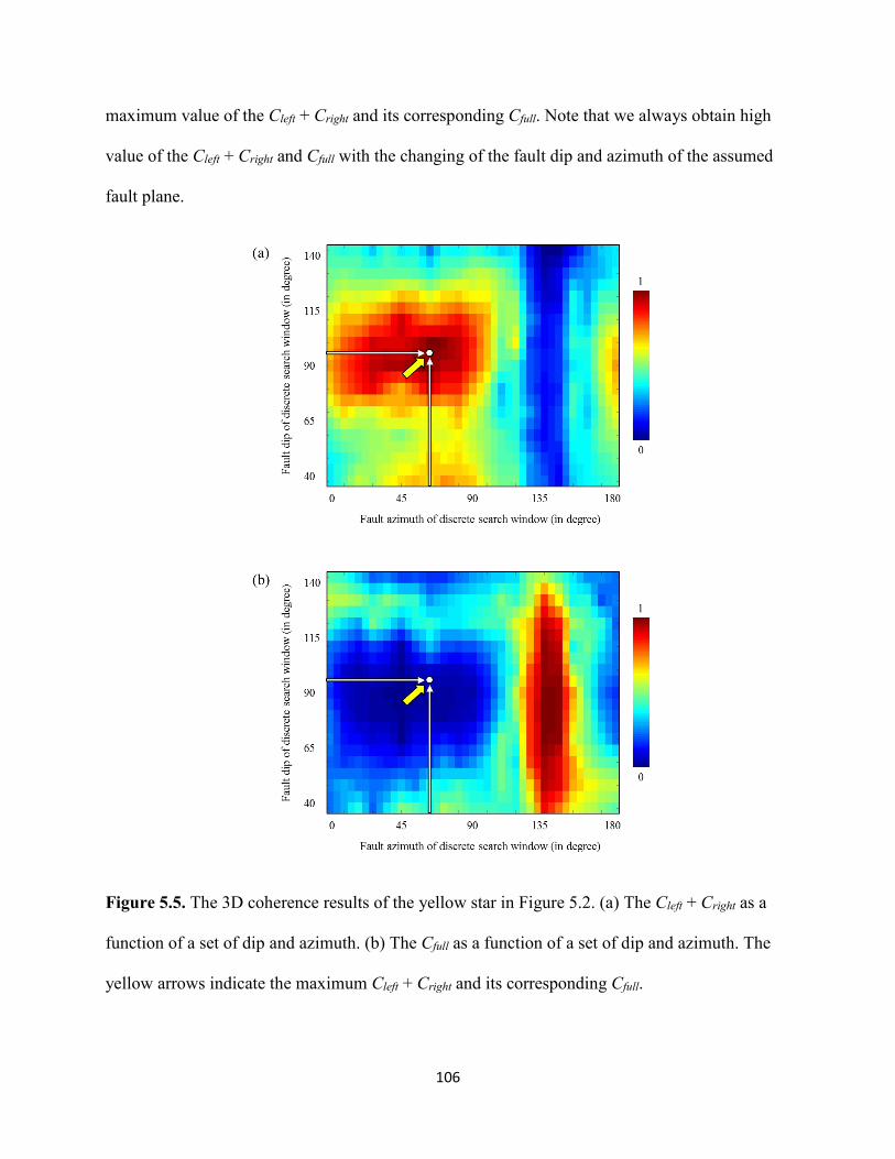
106

maximum value of the Cleft + Cright and its corresponding Cfull. Note that we always obtain high

value of the Cleft + Cright and Cfull with the changing of the fault dip and azimuth of the assumed

fault plane.

Figure 5.5. The 3D coherence results of the yellow star in Figure 5.2. (a) The Cleft + Cright as a

function of a set of dip and azimuth. (b) The Cfull as a function of a set of dip and azimuth. The

yellow arrows indicate the maximum Cleft + Cright and its corresponding Cfull.

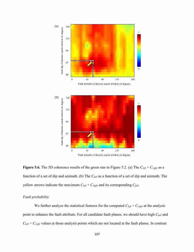
107

Figure 5.6. The 3D coherence results of the green star in Figure 5.2. (a) The Cleft + Cright as a

function of a set of dip and azimuth. (b) The Cfull as a function of a set of dip and azimuth. The

yellow arrows indicate the maximum Cleft + Cright and its corresponding Cfull.

Fault probability

We further analyze the statistical features for the computed Cleft + Cright at the analysis

point to enhance the fault attribute. For all candidate fault planes, we should have high Cfull and

Cleft + Cright values at those analysis points which are not located at the fault planes. In contrast

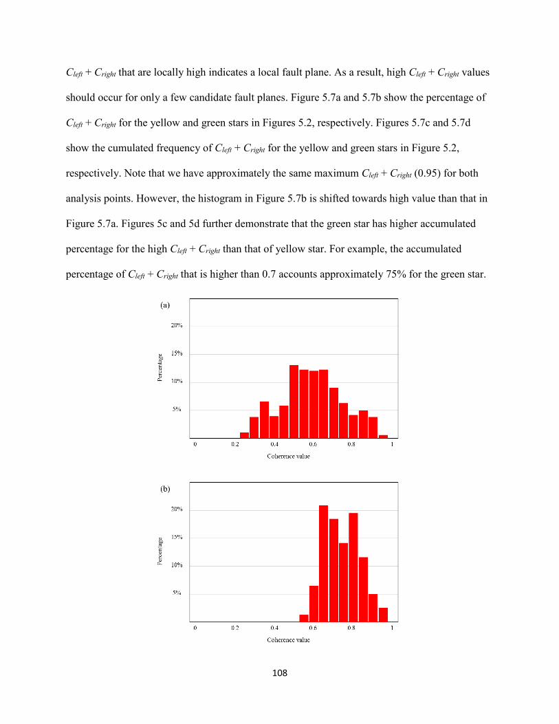
108

Cleft + Cright that are locally high indicates a local fault plane. As a result, high Cleft + Cright values

should occur for only a few candidate fault planes. Figure 5.7a and 5.7b show the percentage of

Cleft + Cright for the yellow and green stars in Figures 5.2, respectively. Figures 5.7c and 5.7d

show the cumulated frequency of Cleft + Cright for the yellow and green stars in Figure 5.2,

respectively. Note that we have approximately the same maximum Cleft + Cright (0.95) for both

analysis points. However, the histogram in Figure 5.7b is shifted towards high value than that in

Figure 5.7a. Figures 5c and 5d further demonstrate that the green star has higher accumulated

percentage for the high Cleft + Cright than that of yellow star. For example, the accumulated

percentage of Cleft + Cright that is higher than 0.7 accounts approximately 75% for the green star.

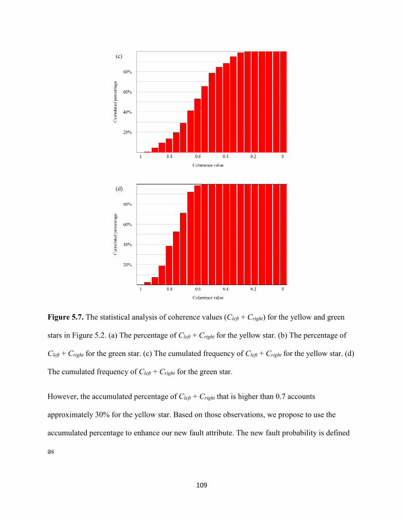
109

Figure 5.7. The statistical analysis of coherence values (Cleft + Cright) for the yellow and green

stars in Figure 5.2. (a) The percentage of Cleft + Cright for the yellow star. (b) The percentage of

Cleft + Cright for the green star. (c) The cumulated frequency of Cleft + Cright for the yellow star. (d)

The cumulated frequency of Cleft + Cright for the green star.

However, the accumulated percentage of Cleft + Cright that is higher than 0.7 accounts

approximately 30% for the yellow star. Based on those observations, we propose to use the

accumulated percentage to enhance our new fault attribute. The new fault probability is defined

as

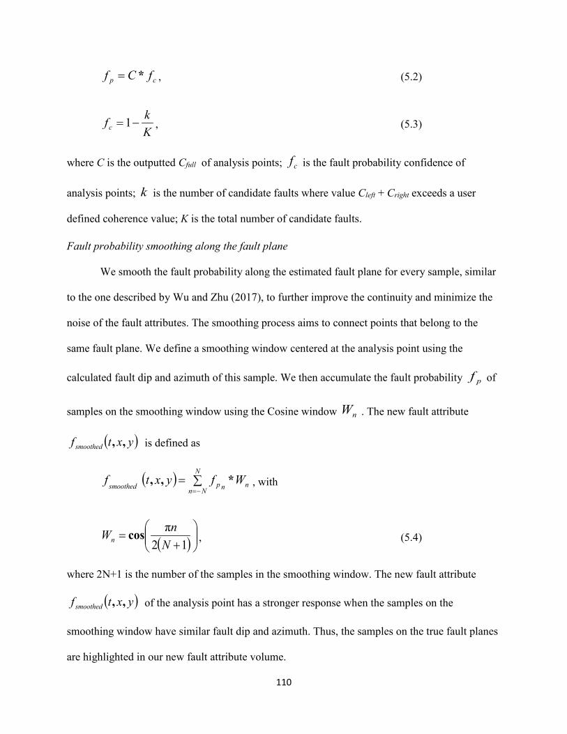
110

cp fCf *= , (5.2)

Kkfc −=1 , (5.3)

where C is the outputted Cfull of analysis points; cf is the fault probability confidence of

analysis points; k is the number of candidate faults where value Cleft + Cright exceeds a user

defined coherence value; K is the total number of candidate faults.

Fault probability smoothing along the fault plane

We smooth the fault probability along the estimated fault plane for every sample, similar

to the one described by Wu and Zhu (2017), to further improve the continuity and minimize the

noise of the fault attributes. The smoothing process aims to connect points that belong to the

same fault plane. We define a smoothing window centered at the analysis point using the

calculated fault dip and azimuth of this sample. We then accumulate the fault probability pf of

samples on the smoothing window using the Cosine window nW . The new fault attribute

( )yxtf smoothed ,, is defined as

( ) ∑=−=

N

Nnnnpsmoothed Wfyxtf *,, , with

( )

+

=12

πN

nWn cos , (5.4)

where 2N+1 is the number of the samples in the smoothing window. The new fault attribute

( )yxtf smoothed ,, of the analysis point has a stronger response when the samples on the

smoothing window have similar fault dip and azimuth. Thus, the samples on the true fault planes

are highlighted in our new fault attribute volume.

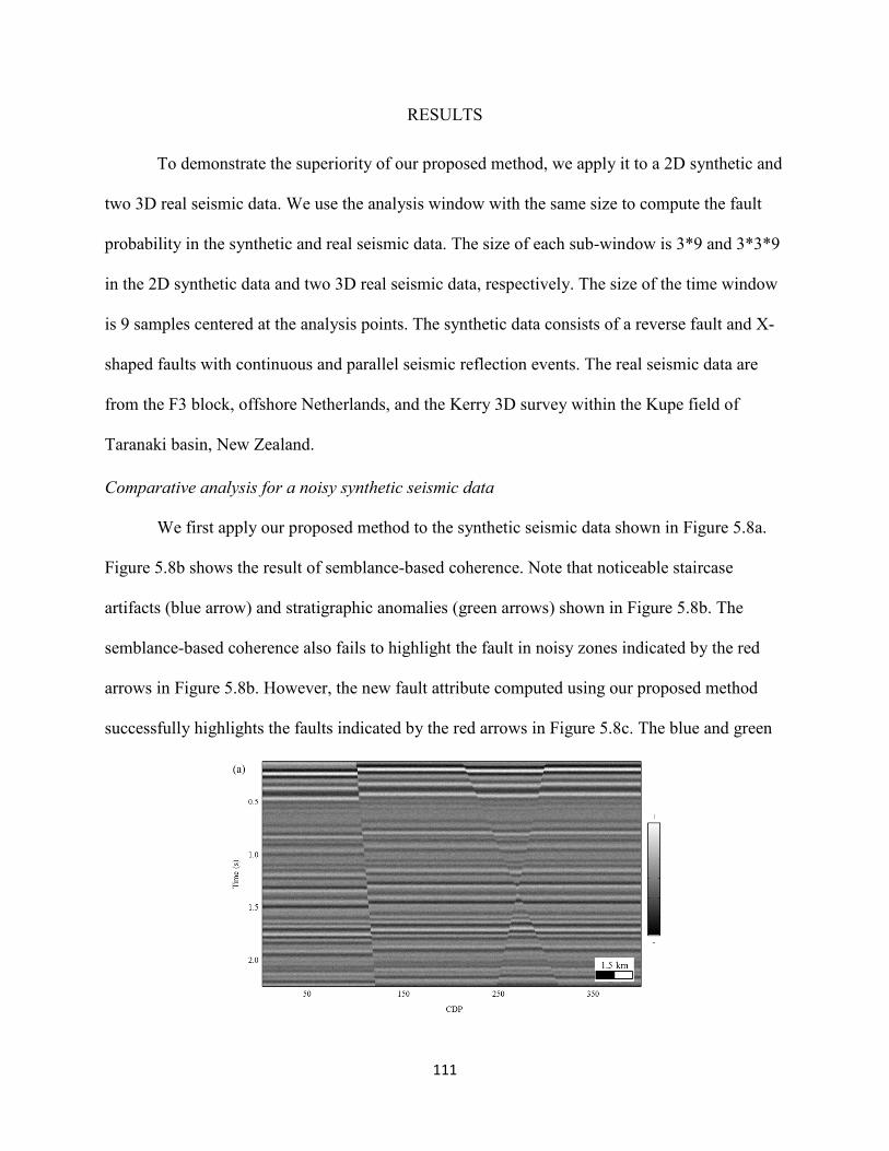
111

RESULTS

To demonstrate the superiority of our proposed method, we apply it to a 2D synthetic and

two 3D real seismic data. We use the analysis window with the same size to compute the fault

probability in the synthetic and real seismic data. The size of each sub-window is 3*9 and 3*3*9

in the 2D synthetic data and two 3D real seismic data, respectively. The size of the time window

is 9 samples centered at the analysis points. The synthetic data consists of a reverse fault and X-

shaped faults with continuous and parallel seismic reflection events. The real seismic data are

from the F3 block, offshore Netherlands, and the Kerry 3D survey within the Kupe field of

Taranaki basin, New Zealand.

Comparative analysis for a noisy synthetic seismic data

We first apply our proposed method to the synthetic seismic data shown in Figure 5.8a.

Figure 5.8b shows the result of semblance-based coherence. Note that noticeable staircase

artifacts (blue arrow) and stratigraphic anomalies (green arrows) shown in Figure 5.8b. The

semblance-based coherence also fails to highlight the fault in noisy zones indicated by the red

arrows in Figure 5.8b. However, the new fault attribute computed using our proposed method

successfully highlights the faults indicated by the red arrows in Figure 5.8c. The blue and green

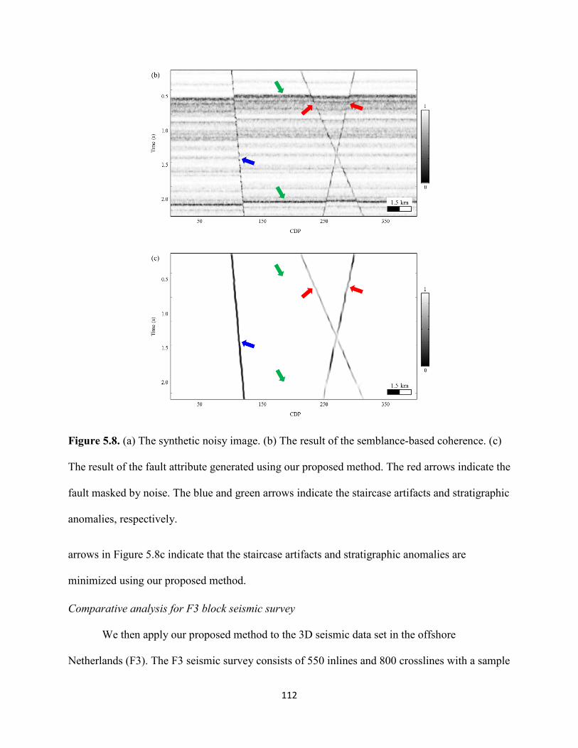
112

Figure 5.8. (a) The synthetic noisy image. (b) The result of the semblance-based coherence. (c)

The result of the fault attribute generated using our proposed method. The red arrows indicate the

fault masked by noise. The blue and green arrows indicate the staircase artifacts and stratigraphic

anomalies, respectively.

arrows in Figure 5.8c indicate that the staircase artifacts and stratigraphic anomalies are

minimized using our proposed method.

Comparative analysis for F3 block seismic survey

We then apply our proposed method to the 3D seismic data set in the offshore

Netherlands (F3). The F3 seismic survey consists of 550 inlines and 800 crosslines with a sample

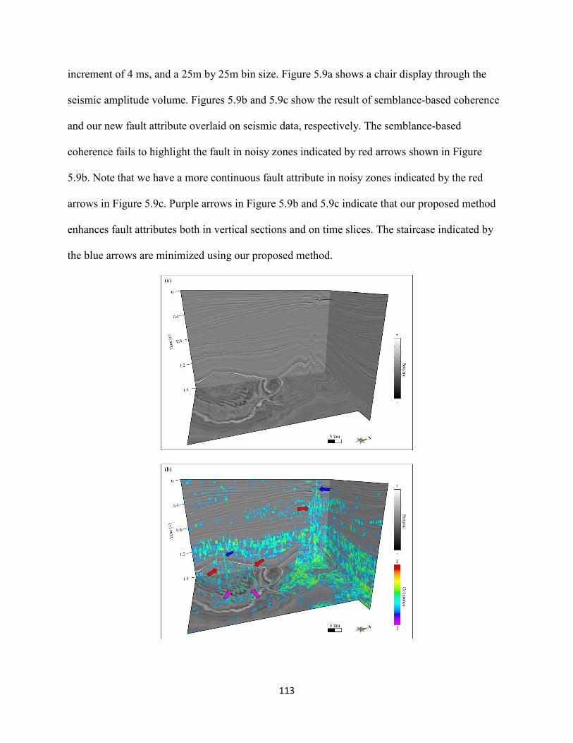
113

increment of 4 ms, and a 25m by 25m bin size. Figure 5.9a shows a chair display through the

seismic amplitude volume. Figures 5.9b and 5.9c show the result of semblance-based coherence

and our new fault attribute overlaid on seismic data, respectively. The semblance-based

coherence fails to highlight the fault in noisy zones indicated by red arrows shown in Figure

5.9b. Note that we have a more continuous fault attribute in noisy zones indicated by the red

arrows in Figure 5.9c. Purple arrows in Figure 5.9b and 5.9c indicate that our proposed method

enhances fault attributes both in vertical sections and on time slices. The staircase indicated by

the blue arrows are minimized using our proposed method.

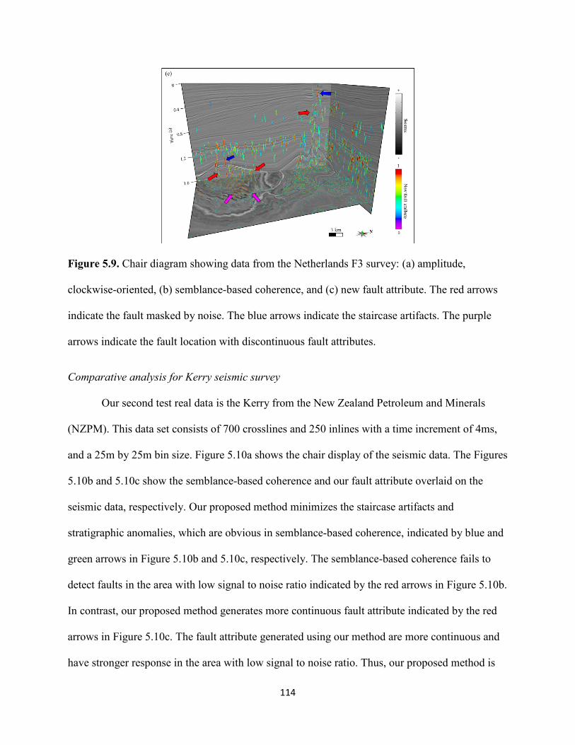
114

Figure 5.9. Chair diagram showing data from the Netherlands F3 survey: (a) amplitude,

clockwise-oriented, (b) semblance-based coherence, and (c) new fault attribute. The red arrows

indicate the fault masked by noise. The blue arrows indicate the staircase artifacts. The purple

arrows indicate the fault location with discontinuous fault attributes.

Comparative analysis for Kerry seismic survey

Our second test real data is the Kerry from the New Zealand Petroleum and Minerals

(NZPM). This data set consists of 700 crosslines and 250 inlines with a time increment of 4ms,

and a 25m by 25m bin size. Figure 5.10a shows the chair display of the seismic data. The Figures

5.10b and 5.10c show the semblance-based coherence and our fault attribute overlaid on the

seismic data, respectively. Our proposed method minimizes the staircase artifacts and

stratigraphic anomalies, which are obvious in semblance-based coherence, indicated by blue and

green arrows in Figure 5.10b and 5.10c, respectively. The semblance-based coherence fails to

detect faults in the area with low signal to noise ratio indicated by the red arrows in Figure 5.10b.

In contrast, our proposed method generates more continuous fault attribute indicated by the red

arrows in Figure 5.10c. The fault attribute generated using our method are more continuous and

have stronger response in the area with low signal to noise ratio. Thus, our proposed method is

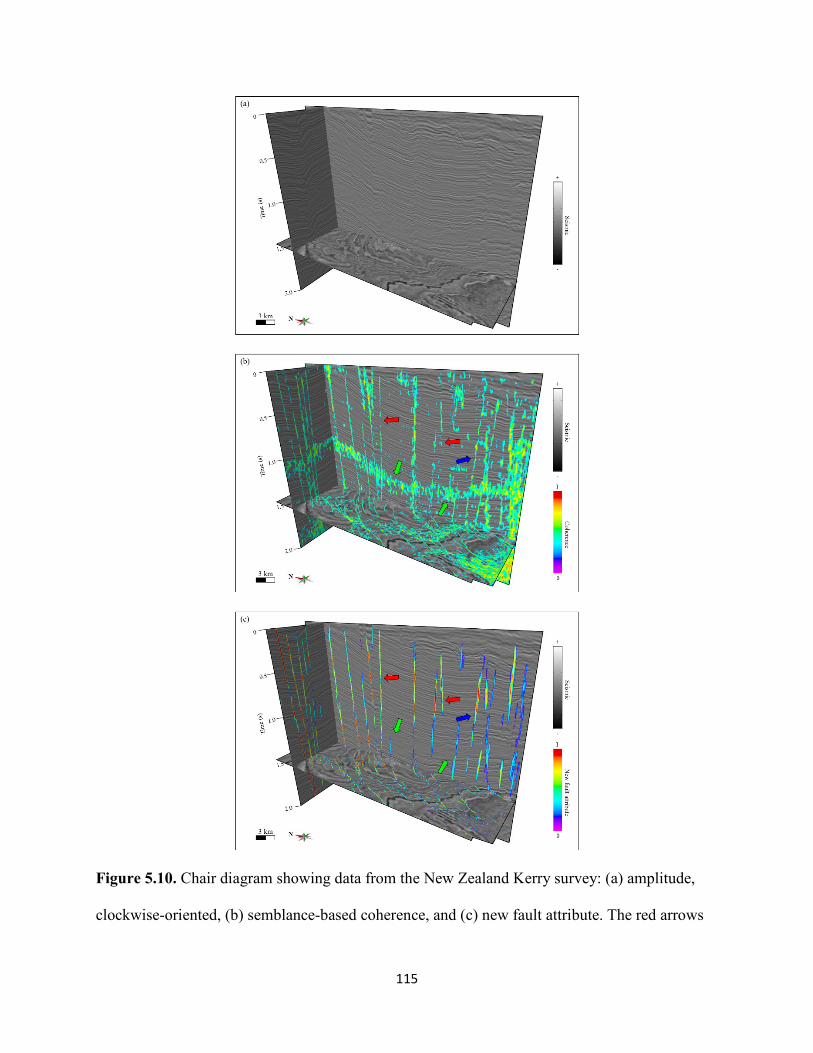
115

Figure 5.10. Chair diagram showing data from the New Zealand Kerry survey: (a) amplitude,

clockwise-oriented, (b) semblance-based coherence, and (c) new fault attribute. The red arrows

116

indicate the fault masked by noise. The blue and green arrows indicate the staircase artifacts and

stratigraphic anomalies, respectively.

superior to conventional coherence method in enhancing faults and depressing staircase artifacts

and stratigraphic anomalies.

DISCUSSION

We assume each analysis sample within the seismic survey may belong to a fault surface

with a single fault dip and azimuth. We obtain the “best” local fault plane by analyzing the

coherence of windowed seismic data divided by the local fault plane. The time analysis window

size of coherence computation is one of the most critical parameters in our method and we

suggest the time analysis of coherence computation window size should approximately equals to

the time duration of one reflection event. The time analysis window size of fault attribute

enhancement is another important parameter in our method and we suggest the time analysis

window size of fault attribute enhancement should approximately equals to the length of the

smallest faults planes within the seismic survey. Our fault model assumes the fault plane is

locally planar. Thus, our method cannot properly address the intersecting points of the X-shaped

faults (Figure 5.8). However, we believe that the smoothing process would properly “replace”

high coherence values with low coherence values for voxels nearby intersecting points of X-

shaped faults if we use the anisotropy smoothing filter. The anisotropic filter would also fail to

replace high coherence values with low coherence values if we have more than two fault sticks

passing through the same voxel. Fortunately, we have rare real cases in which more than two

fault sticks intersect at the same voxel. The seismic data quality definitely affects the

effectiveness of our method. Our method cannot detect the orientation of fault planes if the

semblance of seismic data fails to highlight the faults locations.

117

CONCLUSIONS

We propose to calculate the fault attribute using a 3D scanning strategy constrained by a

local fault model. Our proposed method successfully minimizes staircase artifacts and

stratigraphic anomalies and generates more continuous fault attribute. The proposed method also

precisely highlights faults in the seismic image and has better anti-noise performance. The fault

attribute generated using our proposed method is more continuous along the fault plane in the

inline and crossline sections when compared to that of semblance-based coherence. However, the

computation cost of our proposed method is higher than that of semblance-based coherence. The

computation cost is proportionally increasing with the number of hypothesized local fault plane.

The number of hypothesized local fault plane equals the product between the number of discrete

dip and the number of azimuth of local fault plane. The discrete dip and azimuth of fault plane in

this paper range from -40o to 40o and 0o to 180o, respectively. The increments of dip and azimuth

of fault plane are 10o and 20o, respectively. Thus, our computation cost is roughly 80 times

higher than the conventional semblance-based coherence.

118

REFERENCES

Aqrawi, A. A., and T. H. Boe, 2011, Improved fault segmentation using a dip guided and modified 3D Sobel filter: SEG Technical Program Expanded Abstracts 2011, 999-1003.

Bahorich, M., and S. Farmer, 1995, 3D seismic discontinuity for faults and stratigraphic features: The coherence cube: The Leading Edge, 14(10), 1053-1058.

Bakker, P., L. J. van Vliet, and P.W. Verbeek, 1999, Edge-preserving orientation adaptive filtering: Proceedings, 1999 IEEE Computer Society Conference on Computer Vision and Pattern Recognition, 1, 535-540.

Barnes, A. E., 1996, Theory of 2-D complex seismic trace analysis: Geophysics, 61(1), 264-272.

Cohen, I., N. Coult, and A. A. Vassiliou, 2006, Detection and extraction of fault surfaces in 3D seismic data: Geophysics, 71(4), P21–P27.

Donias, M., C. David, Y. Berthoumieu, O. Lavialle, S. Guillon, and N. Keskes, 2007, New fault attribute based on robust directional scheme: Geophysics, 72(4), P39-P46.

Fehmers, G. C., and C. F. Höcker, 2003, Fast structural interpretation with structure-oriented filtering: Geophysics, 68(4), 1286-1293.

Gersztenkorn, A., and K. J. Marfurt, 1999, Eigenstructure based coherence computations as an aid to 3D structural and stratigraphic mapping: Geophysics, 64(5), 1468–1479.

Hale, D., 2009, Structure-oriented smoothing and semblance: CWP Report, 635, 261-270.

Hale, D., 2013, Methods to compute fault images, extract fault surfaces, and estimate fault throws from 3D seismic images: Geophysics, 78(2), O33–O43.

Luo, Y., M. Marhoon, S. Al-Dossary, and M. Alfaraj, 2002, Edge-preserving smoothing and applications: The Leading Edge, 21(2), 136–158.

Luo, Y., W. G. Higgs, and W. S. Kowalik, 1996, Edge detection and stratigraphic analysis using 3D seismic data: SEG Technical Program Expanded Abstracts 1996, 324-327.

Marfurt, K. J., 2006, Robust estimates of 3D reflector dip and azimuth: Geophysics, 71(4), P29-P40.

Marfurt, K. J., R. L. Kirlin, S. H. Farmer, and M. S. Bahorich, 1998, 3D seismic attributes using a running window semblance-based algorithm: Geophysics, 63(4), 1150-1165.

Marfurt, K. J., V. Sudhakar, A. Gersztenkorn, K. D. Crawford, and S. E. Nissen, 1999, Coherency calculations in the presence of structural dip: Geophysics, 64(1), 104-111.

Marfurt, K. J., and T. Lin, 2017, What Causes those Annoying Stair Step Artifacts on Coherence Volumes?: AAPG explorer, march, 2017.

119

Neff, D. B., J. R. Grismore, and W. A. Lucas, 2000, Automated seismic fault detection and picking: U.S. Patent, 6,018,498.

Pedersen, S., 2007, Image feature extraction: U.S. Patent, 7,203,342.

Pedersen, S., 2011, Image feature extraction: U.S. Patent, 8,055,026.

Qi, J., B. Lyu, A. AlAli, G. Machado, Y. Hu, and K. J. Marfurt, 2018, Image processing of seismic attributes for automatic fault extraction: Geophysics, 84(1), O25-O37.

Qi, J., F. Li, and K. J. Marfurt, 2017, Multiazimuth coherence: Geophysics, 82(6), O83-O89.

Qi, J. and J. Castagna, 2013, Application of a PCA fault-attribute and spectral decomposition in Barnett Shale fault detection: SEG Technical Program Expanded Abstracts 2013, 1421-1425.

Qi, J., G. Machado, and K. J. Marfurt, 2017, A workflow to skeletonize faults and stratigraphic features: Geophysics, 82(4), O57–O70.

Wang, S., S. Yuan, T. Wang, J. Gao, and S. Li, 2018, Three-dimensional geosteering coherence attributes for deep-formation discontinuity detection: Geophysics, 83(6), O105–O113.

Wang, W., J. Gao and K. Li, 2008, Structure-Adaptive anisotropic filter with local structure tensors: 2008 Second International Symposium on Intelligent Information Technology Application, 2, 1005-1010.

Wu, X., 2017, Directional structure-tensor based coherence to detect seismic channels and faults: Geophysics, 82(2), A13-A17.

Wu, X. and D. Hale, 2016, 3D seismic image processing for faults: Geophysics, 81(2), IM1-IM11.

Wu, X., and Z. Zhu, 2017, Methods to enhance seismic faults and construct fault surfaces: Computers & Geosciences, 107, 37-48.

Wu, X., and S. Fomel, 2018, Automatic fault interpretation with optimal surface voting: Geophysics, 83(5), O67–O82.

Yuan, S., Y. Su, T. Wang, J. Wang, and S. Wang, 2018, Geosteering phase attributes: A new detector for the discontinuities of seismic images: IEEE Geoscience and Remote Sensing Letters, 99, 1-5.

Zhang, B., Y. Liu, M. Pelissier, and N. Hemstra, 2014, Semiautomated fault interpretation based on seismic attributes: Interpretation, 2(1), SA11–SA19.

120

CHAPTER 6 FAULT SURFACES CONSTRUCTION THROUGH THE TOPOLOGY ANALYSIS OF

SEISMIC FAULT ATTRIBUTES Yihuai Lou1, Bo Zhang1, Pan Yong2, Huijing Fang3, Yijiang Zhang4 and Danping Cao5

1The University of Alabama, Department of Geological Science. 2Bohai Oilfield Research Institute, Tianjin Branch of CNOOC Ltd. 3China University of Petroleum (Beijing), College of Geosciences.

4Chengdu University of Technology, School of Geophysics. 5China University of Petroleum (East China), School of Geoscience.

This paper was submitted to SEG journal Geophysics in 2020

ABSTRACT

Seismic fault attributes provide geoscientists with alternative images of faults that can be

used as components in unraveling the structural deformation history of subsurface. However,

seismic fault attributes can only highlight possible fault locations and cannot provide fault

surfaces that are compulsory inputs for structural modeling. We propose to automatically

construct the fault surfaces by analyzing the topological relationship of seismic fault attributes on

inline, crossline, and time slices. Our algorithm consists of three main steps: (1) obtaining fault

sticks on inline, crossline, and time slices, (2) grouping the fault sticks by analyzing the

topological relationships between the faults sticks on inline, crossline, and time slices, and (3)

generating fault surface patches by merging the fault sticks time slice by time slice through the

topology analysis. Our algorithm contains one optional step: manually merging the fault patches

if needed. We tested our algorithm on open access seismic data and the proposed workflow

accurately generates fault surfaces for all the faults including conjugate faults in the seismic data.

In addition, the algorithm can compute the fault parameters such as fault dip and strike.

121

INTRODUCTION

Researchers have developed seismic fault attributes to assist in seismic fault

interpretations in 3D seismic surveys. Research related to seismic fault interpretation can be

classified into two categories. The first category generates prototype algorithms for seismic fault

attributes. Luo et al. (1996) detect faults and analysis stratigraphic boundaries by employing

complex traces analysis to 3D seismic data. Marfurt et al. (1998) propose the semblance-based

coherence algorithm to detect faults using a suite of sampling windows. Gersztenkorn and

Marfurt (1999) propose the Eigenstructure-based coherence algorithm by analyzing the

Eigenstructure of seismic traces in the sampling window. Marfurt (2006) further improve the

semblance-based coherence by employing a multiple window Kuwahara searching method. The

gradient structure tensor (GST) is also used to detect discontinuities features in seismic images

by employing the eigenvector with largest eigenvalue (Bakker et al., 1999; Fehmers and

Hoecker, 2003; Wu, 2017). Hale (2013) compute the fault likelihood by scanning all possible

fault orientations. Qi et al. (2017a) compute the Multi-azimuth coherence by using azimuthally

limited seismic data volumes. Other seismic attributes, such as edge-preserving smoothing (Luo

et al., 2002), curvature (Al-Dossary and marfurt, 2006; Di and Gao, 2016), and gradient

magnitude (Aqrawi and Boe, 2011) have been proposed to detect faults. However, it is difficult

to track fault features continuously in the fault attributes. Undesired sequence artifacts and

staircases are also common in the seismic images with low signal-to-noise ratio.

The second category aims to enhance the seismic fault attributes. Pedersen et al. (2002,

2003) propose the Ant tracking algorithm to enhance fault features along paths of “artificial

ants”. AlBinHassan and Marfurt (2003) enhance the continuity of faults and fractures by using

the Hough transforms algorithm. Qi and Castagna (2013) improve the accuracy of fault detection

122

attributes by combing the principal component analysis (PCA). Qi et al. (2017b, 2018) further

improve the coherence attribute by skeletonizing fault images along fault planes. Lou et al.

(2019) generate the fault attribute without staircase artifacts and undesired sequence artifacts by

using a local fault model. Researchers also enhance the fault features by smoothing fault

attributes along fault dip and azimuth (Neff et al., 2000; Cohen et al., 2006; Hale, 2009).

Researchers have tried to automatically form the seismic fault surfaces using seismic

fault attributes. Zhang et al. (2014) generate fault surfaces by applying the vein pattern

recognition algorithm to the coherence attributes. Wu and Hale (2016) generate fault surfaces

using a linked data structure from 3D seismic images. Wu and Fomel (2018) propose the optimal

surface voting algorithm to generate fault surfaces, and calculate corresponding fault dip and

azimuth. However, it is still a challenge to automatically generate fault surfaces for conjugate

faults, especially for the faults which have a dip variation with locations.

In this paper, we propose a new workflow to automatically generate fault surfaces. Our

method consists of three steps and is based on analyzing the features of fault attributes on 2D

slices. The algorithm begins with generating “initial” fault sticks on inline, crossline, and time

slices from the seismic fault attributes using a user-defined threshold. The algorithm then

computes the azimuth of initial fault sticks on time slice and the dip of initial fault sticks on

vertical slices by integrating a Kuwahara window and the weighted principal component analysis

(WPCA). We obtain refined fault sticks by analyzing the azimuth and dip of the initial fault

sticks. The refined fault sticks are grouped to the same group if they are connected with each

other directly or indirectly. We finally produce fault surfaces from the grouped fault sticks by

analyzing their topological relationships. We illustrate our workflow step by step by applying it

on the poststack seismic survey Kerry acquired from offshore New Zealand.

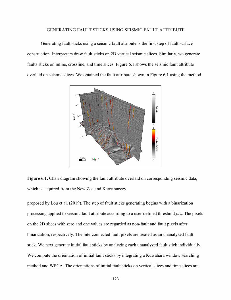
123

GENERATING FAULT STICKS USING SEISMIC FAULT ATTRIBUTE

Generating fault sticks using a seismic fault attribute is the first step of fault surface

construction. Interpreters draw fault sticks on 2D vertical seismic slices. Similarly, we generate

faults sticks on inline, crossline, and time slices. Figure 6.1 shows the seismic fault attribute

overlaid on seismic slices. We obtained the fault attribute shown in Figure 6.1 using the method

Figure 6.1. Chair diagram showing the fault attribute overlaid on corresponding seismic data,

which is acquired from the New Zealand Kerry survey.

proposed by Lou et al. (2019). The step of fault sticks generating begins with a binarization

processing applied to seismic fault attribute according to a user-defined threshold fmin. The pixels

on the 2D slices with zero and one values are regarded as non-fault and fault pixels after

binarization, respectively. The interconnected fault pixels are treated as an unanalyzed fault

stick. We next generate initial fault sticks by analyzing each unanalyzed fault stick individually.

We compute the orientation of initial fault sticks by integrating a Kuwahara window searching

method and WPCA. The orientations of initial fault sticks on vertical slices and time slices are

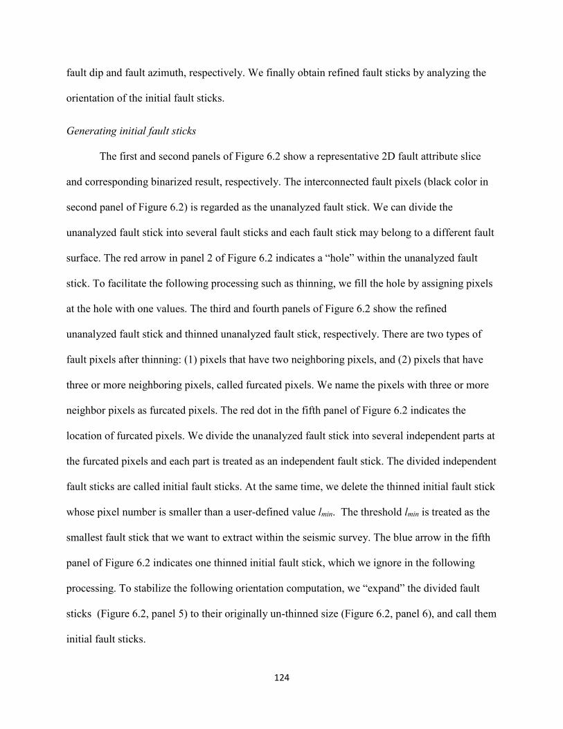
124

fault dip and fault azimuth, respectively. We finally obtain refined fault sticks by analyzing the

orientation of the initial fault sticks.

Generating initial fault sticks

The first and second panels of Figure 6.2 show a representative 2D fault attribute slice

and corresponding binarized result, respectively. The interconnected fault pixels (black color in

second panel of Figure 6.2) is regarded as the unanalyzed fault stick. We can divide the

unanalyzed fault stick into several fault sticks and each fault stick may belong to a different fault

surface. The red arrow in panel 2 of Figure 6.2 indicates a “hole” within the unanalyzed fault

stick. To facilitate the following processing such as thinning, we fill the hole by assigning pixels

at the hole with one values. The third and fourth panels of Figure 6.2 show the refined

unanalyzed fault stick and thinned unanalyzed fault stick, respectively. There are two types of

fault pixels after thinning: (1) pixels that have two neighboring pixels, and (2) pixels that have

three or more neighboring pixels, called furcated pixels. We name the pixels with three or more

neighbor pixels as furcated pixels. The red dot in the fifth panel of Figure 6.2 indicates the

location of furcated pixels. We divide the unanalyzed fault stick into several independent parts at

the furcated pixels and each part is treated as an independent fault stick. The divided independent

fault sticks are called initial fault sticks. At the same time, we delete the thinned initial fault stick

whose pixel number is smaller than a user-defined value lmin. The threshold lmin is treated as the

smallest fault stick that we want to extract within the seismic survey. The blue arrow in the fifth

panel of Figure 6.2 indicates one thinned initial fault stick, which we ignore in the following

processing. To stabilize the following orientation computation, we “expand” the divided fault

sticks (Figure 6.2, panel 5) to their originally un-thinned size (Figure 6.2, panel 6), and call them

initial fault sticks.

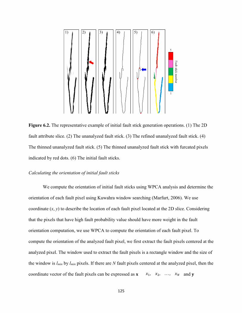
125

Figure 6.2. The representative example of initial fault stick generation operations. (1) The 2D

fault attribute slice. (2) The unanalyzed fault stick. (3) The refined unanalyzed fault stick. (4)

The thinned unanalyzed fault stick. (5) The thinned unanalyzed fault stick with furcated pixels

indicated by red dots. (6) The initial fault sticks.

Calculating the orientation of initial fault sticks

We compute the orientation of initial fault sticks using WPCA analysis and determine the

orientation of each fault pixel using Kuwahra window searching (Marfurt, 2006). We use

coordinate (x, y) to describe the location of each fault pixel located at the 2D slice. Considering

that the pixels that have high fault probability value should have more weight in the fault

orientation computation, we use WPCA to compute the orientation of each fault pixel. To

compute the orientation of the analyzed fault pixel, we first extract the fault pixels centered at the

analyzed pixel. The window used to extract the fault pixels is a rectangle window and the size of

the window is lmin by lmin pixels. If there are N fault pixels centered at the analyzed pixel, then the

coordinate vector of the fault pixels can be expressed as 𝐱𝐱 = (𝑥𝑥1, 𝑥𝑥2, . . . , 𝑥𝑥𝑁𝑁) and 𝐲𝐲 =

126

(𝑦𝑦1, 𝑦𝑦2, . . . , 𝑦𝑦𝑁𝑁). The seismic fault attribute values for the fault pixels are expressed as 𝐬𝐬 =

(𝑠𝑠1, 𝑠𝑠2, . . . , 𝑠𝑠𝑁𝑁). WPCA implements a weighted PCA procedure to each fault pixel within the

analysis window by adding a weight to the covariance matrix (Fan et al., 2011) using

𝐂𝐂𝑖𝑖 = 1𝑁𝑁−1

�cov𝑖𝑖(𝐱𝐱, 𝐱𝐱) cov𝑖𝑖(𝐱𝐱,𝐲𝐲)cov𝑖𝑖(𝐲𝐲,𝐱𝐱) cov𝑖𝑖(𝐲𝐲, 𝐲𝐲)�, (6.1)

where the covariance elements cov𝑖𝑖(𝐱𝐱, 𝐱𝐱), cov𝑖𝑖(𝐱𝐱,𝐲𝐲), cov𝑖𝑖(𝐲𝐲, 𝐱𝐱), and cov𝑖𝑖(𝐲𝐲, 𝐲𝐲) are defined

as following

cov𝑖𝑖(𝐱𝐱, 𝐱𝐱) =� 𝑠𝑠𝑖𝑖(𝑥𝑥𝑖𝑖−�̅�𝑥)𝑁𝑁

𝑖𝑖=1 (𝑥𝑥𝑖𝑖−�̅�𝑥)

𝑁𝑁−1, (6.2a)

cov𝑖𝑖(𝐱𝐱, 𝐲𝐲) =� 𝑠𝑠𝑖𝑖(𝑥𝑥𝑖𝑖−�̅�𝑥)𝑁𝑁

𝑖𝑖=1 (𝑦𝑦𝑖𝑖−𝑦𝑦�)

𝑁𝑁−1, (6.2b)

cov𝑖𝑖(𝐲𝐲, 𝐱𝐱) =� 𝑠𝑠𝑖𝑖(𝑦𝑦𝑖𝑖−𝑦𝑦�)𝑁𝑁

𝑖𝑖=1 (𝑥𝑥𝑖𝑖−�̅�𝑥)

𝑁𝑁−1, (6.2c)

cov𝑖𝑖(𝐲𝐲, 𝐲𝐲) =� 𝑠𝑠𝑖𝑖(𝑦𝑦𝑖𝑖−𝑦𝑦�)𝑁𝑁

𝑖𝑖=1 (𝑦𝑦𝑖𝑖−𝑦𝑦�)

𝑁𝑁−1, (6.2d)

where �̅�𝑥 and 𝑦𝑦� are average value of x and y, respectively. We obtain the eigenvalue and

eigenvector of covariance matrix shown in Equation 5.1 by applying the Eigen-decomposition

𝐂𝐂𝑖𝑖 = 𝜆𝜆𝑢𝑢𝐮𝐮𝐮𝐮𝐼𝐼 + 𝜆𝜆𝑣𝑣𝐯𝐯𝐯𝐯𝐼𝐼 = �𝜆𝜆𝑢𝑢 00 𝜆𝜆𝑣𝑣

� �𝐮𝐮𝐼𝐼

𝐯𝐯𝐼𝐼�, (6.3)

where 𝜆𝜆𝑢𝑢 and 𝜆𝜆𝑣𝑣 are eigenvalues satisfied 𝜆𝜆𝑢𝑢 ≥ 𝜆𝜆𝑣𝑣 ≥ 0; u and v are the corresponding

normalized eigenvectors. The dominant eigenvector u is regarded to be perpendicular to the fault

stick at the analysis pixel. The fault orientation p and confidence q of the analysis pixel is

defined as

𝑝𝑝 = 𝐮𝐮𝑦𝑦𝐮𝐮𝑥𝑥

, (6.4a)

127

𝑞𝑞 = 𝜆𝜆𝑢𝑢𝜆𝜆𝑢𝑢+𝜆𝜆𝑣𝑣

. (6.4b)

We obtain the orientation 𝐩𝐩 = (𝑝𝑝1, 𝑝𝑝2, . . . , 𝑝𝑝𝑁𝑁) and corresponding confidence 𝐪𝐪 =

(𝑞𝑞1, 𝑞𝑞2, . . . , 𝑞𝑞𝑁𝑁) for all the pixels of the fault stick by applying the method illustrated by

equations 5.1, 5.2, 5.3, and 5.4. We refine the calculated orientation of fault sticks by applying

the Kuwahara window searching to the confidence vector q. The window size for the Kuwahara

window searching is lmin by lmin pixels.

In Figures 6.3a and 6.3b, the red dots in panel 1 are the same representative analysis fault

pixels. The blue rectangle in Figure 6.3a is the analysis window used for fault orientation

computation if we only consider whether a pixel is a fault pixel (The traditional analysis

window). The blue rectangle in Figure 6.3b is the analysis window (the most coherent window)

used for fault orientation computation by considering which fault stick does the analysis pixel

belongs to. Note that the traditional analysis window in the second panel of Figure 6.3a includes

fault pixels belonging to two faults sticks and their orientation differs with each other. As a

result, we may obtain an inaccurate orientation value if the analysis window includes furcated

fault pixels. However, our new analysis window only contains faults pixels belonging to the

same fault stick. Thus, we will obtain a more accurate orientation estimation. The third panels in

Figures 6.3a and 6.3b show the computed orientation using the traditional analysis window and

our new strategy, respectively. The red arrows in Figures 6.3a and 6.3b indicate the notably

improved orientation estimation. Figure 6.4 shows the refined fault orientation after applying the

Kuwahara window searching to the calculated orientation shown in the third panel of Figure

6.3b. The refined fault orientation (indicated by the blue arrows) in Figure 6.4 is more uniform

and accurate than the calculated fault orientation in the third panel of Figure 6.3b.

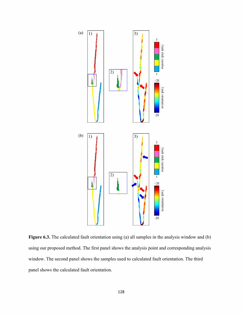
128

Figure 6.3. The calculated fault orientation using (a) all samples in the analysis window and (b)

using our proposed method. The first panel shows the analysis point and corresponding analysis

window. The second panel shows the samples used to calculated fault orientation. The third

panel shows the calculated fault orientation.

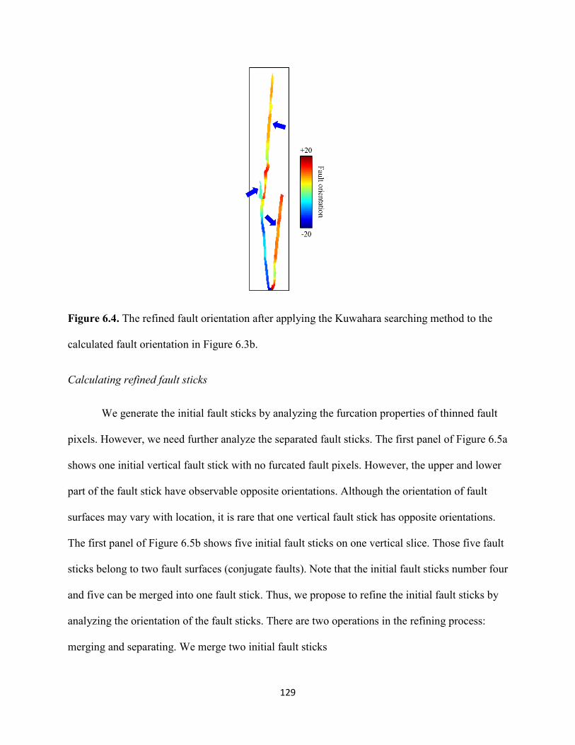
129

Figure 6.4. The refined fault orientation after applying the Kuwahara searching method to the

calculated fault orientation in Figure 6.3b.

Calculating refined fault sticks

We generate the initial fault sticks by analyzing the furcation properties of thinned fault

pixels. However, we need further analyze the separated fault sticks. The first panel of Figure 6.5a

shows one initial vertical fault stick with no furcated fault pixels. However, the upper and lower

part of the fault stick have observable opposite orientations. Although the orientation of fault

surfaces may vary with location, it is rare that one vertical fault stick has opposite orientations.

The first panel of Figure 6.5b shows five initial fault sticks on one vertical slice. Those five fault

sticks belong to two fault surfaces (conjugate faults). Note that the initial fault sticks number four

and five can be merged into one fault stick. Thus, we propose to refine the initial fault sticks by

analyzing the orientation of the fault sticks. There are two operations in the refining process:

merging and separating. We merge two initial fault sticks

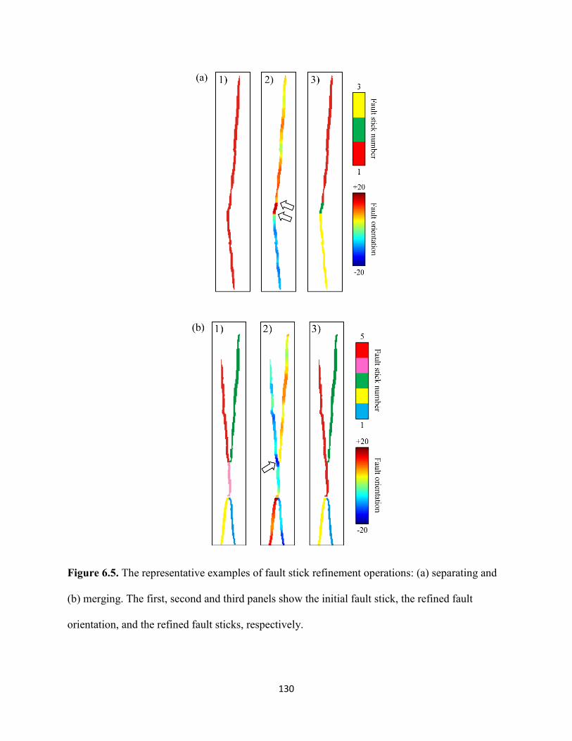
130

Figure 6.5. The representative examples of fault stick refinement operations: (a) separating and

(b) merging. The first, second and third panels show the initial fault stick, the refined fault

orientation, and the refined fault sticks, respectively.

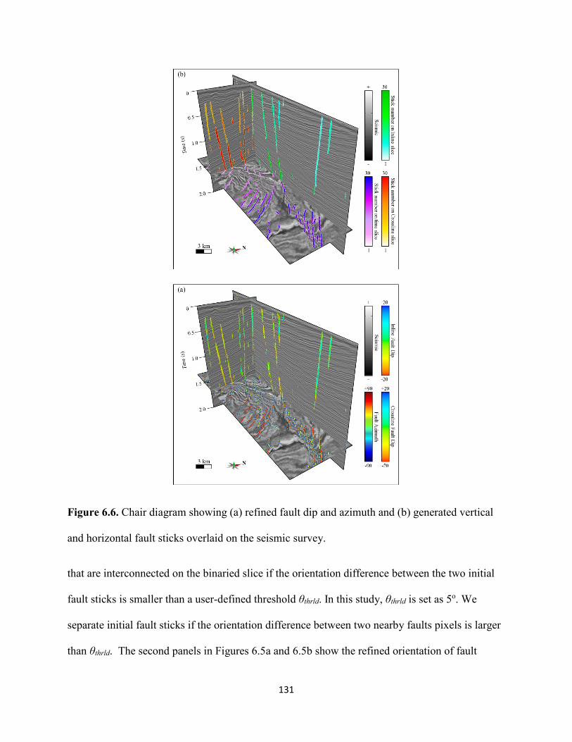
131

Figure 6.6. Chair diagram showing (a) refined fault dip and azimuth and (b) generated vertical

and horizontal fault sticks overlaid on the seismic survey.

that are interconnected on the binaried slice if the orientation difference between the two initial

fault sticks is smaller than a user-defined threshold θthrld. In this study, θthrld is set as 5o. We

separate initial fault sticks if the orientation difference between two nearby faults pixels is larger

than θthrld. The second panels in Figures 6.5a and 6.5b show the refined orientation of fault

132

sticks. The white arrows in the second panel of Figure 6.5a indicate separate locations of initial

fault sticks. The white arrow in the second panel of Figure 6.5b indicate the merging location.

The third panels of Figures 6.5a and 6.5b show the refined fault sticks by using the orientation

value shown in second panel of Figure 6.5.

We apply our proposed fault sticks refining step to every vertical and horizontal seismic

slices. The refined fault sticks on vertical (inline and crossline) and horizontal (time slice) slices

are named as vertical fault sticks and horizontal fault sticks, respectively. We give a unique fault

stick number to each refined fault stick on vertical and time slices. Figure 6.6a shows the refined

fault azimuth on time slice and fault dip on vertical slices. Figure 6.6b shows the refined fault

sticks on time and vertical slices. As a result, each time sample of seismic traces has three fault

stick numbers if the time sample is located at the fault location.

GROUPING FAULT STICKS

To facilitate the following fault surface construction, we propose to group the fault sticks

(Figure 6.7) into different groups prior the fault surface construction. The fault sticks within the

same group should belong to the same surface if there is no intersection between two or more

fault surfaces. The longest horizontal fault stick within the stick bank is regarded as the “center”

stick for generating a group of fault sticks. The workflow then collects all vertical fault sticks

that are connected with the center stick. We form new center fault sticks by merging all the

horizontal fault sticks that are connected with the collected vertical fault sticks. The grouping

process iteratively collects vertical fault sticks and merges horizontal fault sticks until there are

no more fault sticks connected with any of the fault sticks in current group. We then give a group

number to the grouped fault sticks and exclude the fault sticks that already are merged with the

current group. We next locate the longest horizontal fault stick within the stick bank and repeat

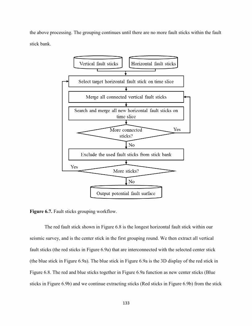
133

the above processing. The grouping continues until there are no more fault sticks within the fault

stick bank.

Figure 6.7. Fault sticks grouping workflow.

The red fault stick shown in Figure 6.8 is the longest horizontal fault stick within our

seismic survey, and is the center stick in the first grouping round. We then extract all vertical

fault sticks (the red sticks in Figure 6.9a) that are interconnected with the selected center stick

(the blue stick in Figure 6.9a). The blue stick in Figure 6.9a is the 3D display of the red stick in

Figure 6.8. The red and blue sticks together in Figure 6.9a function as new center sticks (Blue

sticks in Figure 6.9b) and we continue extracting sticks (Red sticks in Figure 6.9b) from the stick

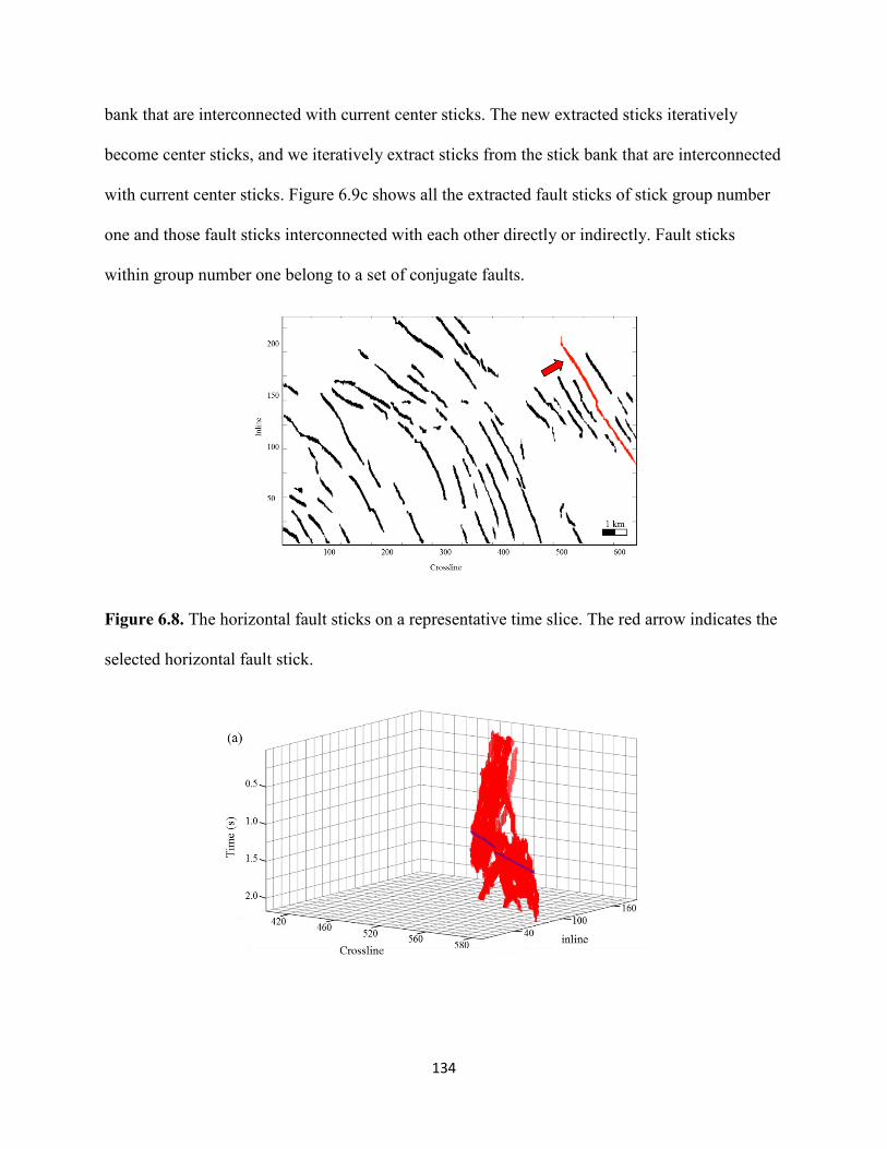
134

bank that are interconnected with current center sticks. The new extracted sticks iteratively

become center sticks, and we iteratively extract sticks from the stick bank that are interconnected

with current center sticks. Figure 6.9c shows all the extracted fault sticks of stick group number

one and those fault sticks interconnected with each other directly or indirectly. Fault sticks

within group number one belong to a set of conjugate faults.

Figure 6.8. The horizontal fault sticks on a representative time slice. The red arrow indicates the

selected horizontal fault stick.

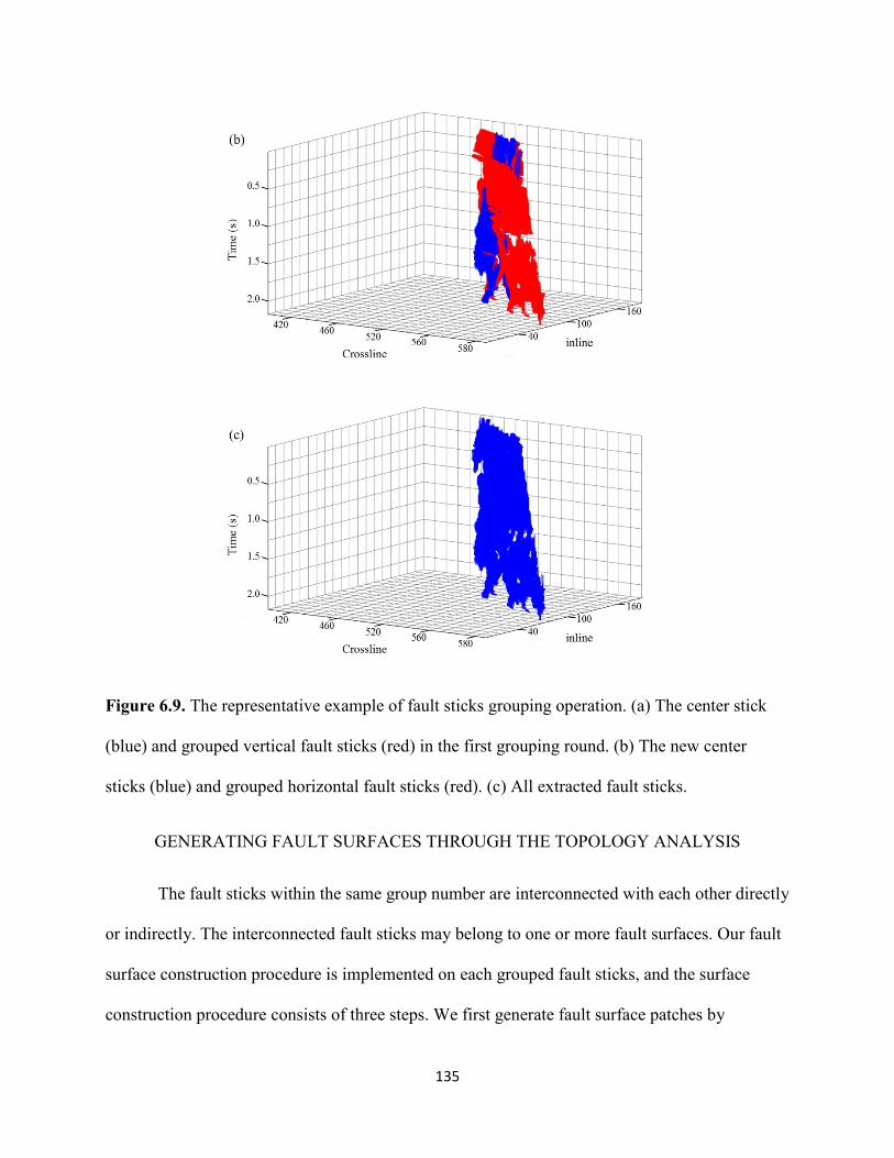
135

Figure 6.9. The representative example of fault sticks grouping operation. (a) The center stick

(blue) and grouped vertical fault sticks (red) in the first grouping round. (b) The new center

sticks (blue) and grouped horizontal fault sticks (red). (c) All extracted fault sticks.

GENERATING FAULT SURFACES THROUGH THE TOPOLOGY ANALYSIS

The fault sticks within the same group number are interconnected with each other directly

or indirectly. The interconnected fault sticks may belong to one or more fault surfaces. Our fault

surface construction procedure is implemented on each grouped fault sticks, and the surface

construction procedure consists of three steps. We first generate fault surface patches by

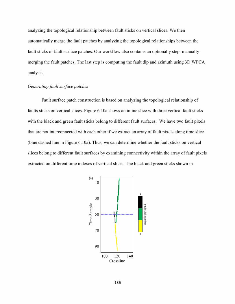
136

analyzing the topological relationship between fault sticks on vertical slices. We then

automatically merge the fault patches by analyzing the topological relationships between the

fault sticks of fault surface patches. Our workflow also contains an optionally step: manually

merging the fault patches. The last step is computing the fault dip and azimuth using 3D WPCA

analysis.

Generating fault surface patches

Fault surface patch construction is based on analyzing the topological relationship of

faults sticks on vertical slices. Figure 6.10a shows an inline slice with three vertical fault sticks

with the black and green fault sticks belong to different fault surfaces. We have two fault pixels

that are not interconnected with each other if we extract an array of fault pixels along time slice

(blue dashed line in Figure 6.10a). Thus, we can determine whether the fault sticks on vertical

slices belong to different fault surfaces by examining connectivity within the array of fault pixels

extracted on different time indexes of vertical slices. The black and green sticks shown in

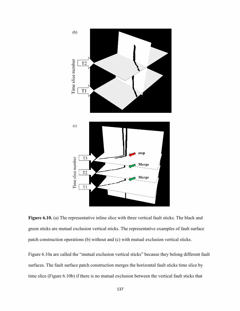
137

Figure 6.10. (a) The representative inline slice with three vertical fault sticks. The black and

green sticks are mutual exclusion vertical sticks. The representative examples of fault surface

patch construction operations (b) without and (c) with mutual exclusion vertical sticks.

Figure 6.10a are called the “mutual exclusion vertical sticks” because they belong different fault

surfaces. The fault surface patch construction merges the horizontal fault sticks time slice by

time slice (Figure 6.10b) if there is no mutual exclusion between the vertical fault sticks that

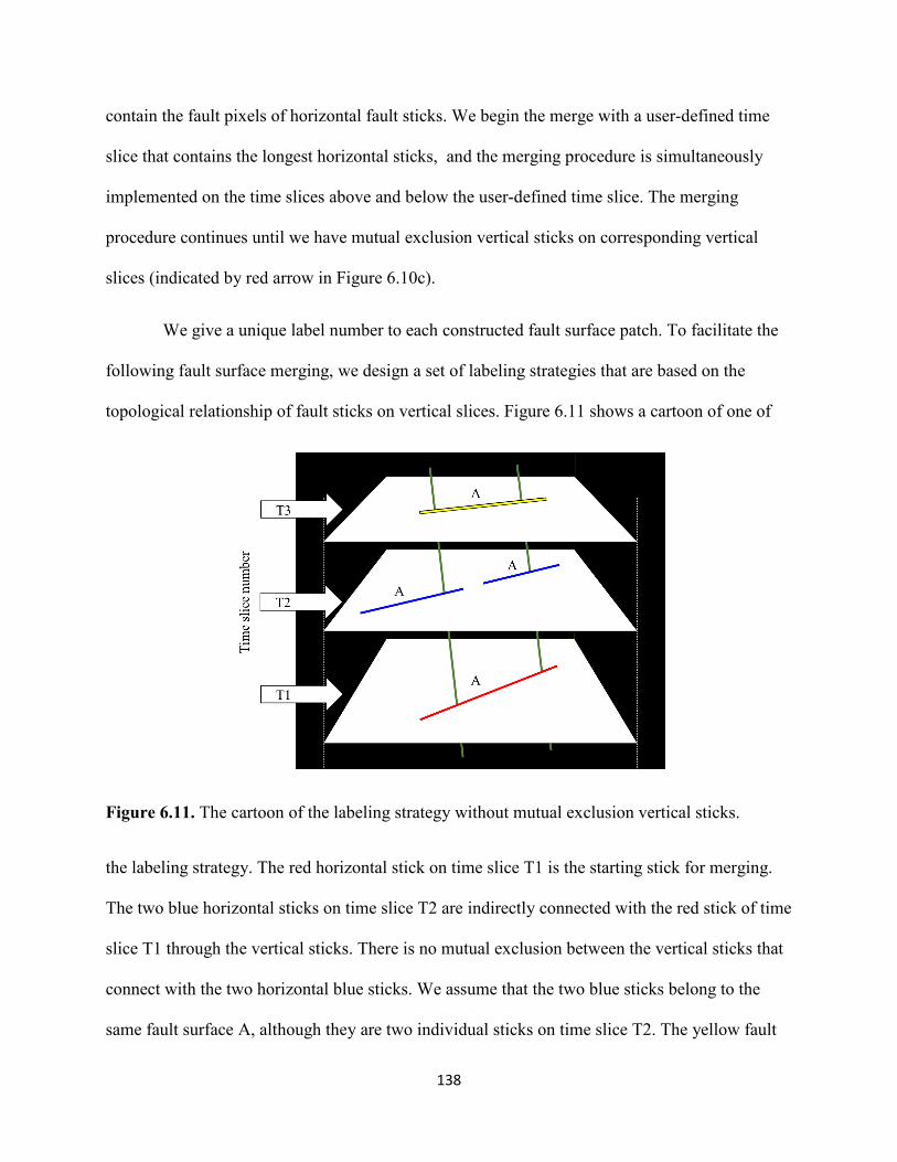
138

contain the fault pixels of horizontal fault sticks. We begin the merge with a user-defined time

slice that contains the longest horizontal sticks, and the merging procedure is simultaneously

implemented on the time slices above and below the user-defined time slice. The merging

procedure continues until we have mutual exclusion vertical sticks on corresponding vertical

slices (indicated by red arrow in Figure 6.10c).

We give a unique label number to each constructed fault surface patch. To facilitate the

following fault surface merging, we design a set of labeling strategies that are based on the

topological relationship of fault sticks on vertical slices. Figure 6.11 shows a cartoon of one of

Figure 6.11. The cartoon of the labeling strategy without mutual exclusion vertical sticks.

the labeling strategy. The red horizontal stick on time slice T1 is the starting stick for merging.

The two blue horizontal sticks on time slice T2 are indirectly connected with the red stick of time

slice T1 through the vertical sticks. There is no mutual exclusion between the vertical sticks that

connect with the two horizontal blue sticks. We assume that the two blue sticks belong to the

same fault surface A, although they are two individual sticks on time slice T2. The yellow fault

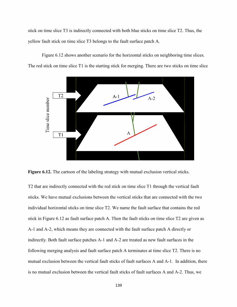
139

stick on time slice T3 is indirectly connected with both blue sticks on time slice T2. Thus, the

yellow fault stick on time slice T3 belongs to the fault surface patch A.

Figure 6.12 shows another scenario for the horizontal sticks on neighboring time slices.

The red stick on time slice T1 is the starting stick for merging. There are two sticks on time slice

Figure 6.12. The cartoon of the labeling strategy with mutual exclusion vertical sticks.

T2 that are indirectly connected with the red stick on time slice T1 through the vertical fault

sticks. We have mutual exclusions between the vertical sticks that are connected with the two

individual horizontal sticks on time slice T2. We name the fault surface that contains the red

stick in Figure 6.12 as fault surface patch A. Then the fault sticks on time slice T2 are given as

A-1 and A-2, which means they are connected with the fault surface patch A directly or

indirectly. Both fault surface patches A-1 and A-2 are treated as new fault surfaces in the

following merging analysis and fault surface patch A terminates at time slice T2. There is no

mutual exclusion between the vertical fault sticks of fault surfaces A and A-1. In addition, there

is no mutual exclusion between the vertical fault sticks of fault surfaces A and A-2. Thus, we

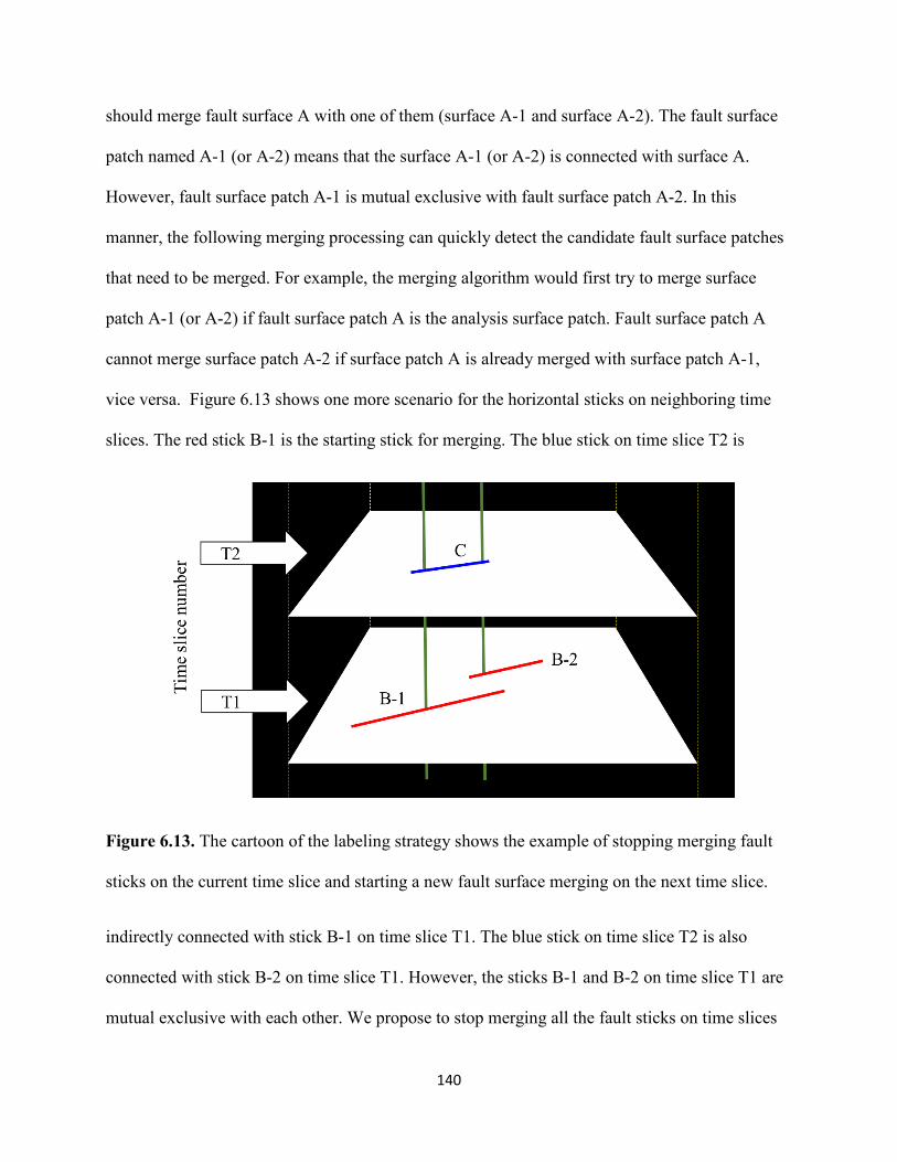
140

should merge fault surface A with one of them (surface A-1 and surface A-2). The fault surface

patch named A-1 (or A-2) means that the surface A-1 (or A-2) is connected with surface A.

However, fault surface patch A-1 is mutual exclusive with fault surface patch A-2. In this

manner, the following merging processing can quickly detect the candidate fault surface patches

that need to be merged. For example, the merging algorithm would first try to merge surface

patch A-1 (or A-2) if fault surface patch A is the analysis surface patch. Fault surface patch A

cannot merge surface patch A-2 if surface patch A is already merged with surface patch A-1,

vice versa. Figure 6.13 shows one more scenario for the horizontal sticks on neighboring time

slices. The red stick B-1 is the starting stick for merging. The blue stick on time slice T2 is

Figure 6.13. The cartoon of the labeling strategy shows the example of stopping merging fault

sticks on the current time slice and starting a new fault surface merging on the next time slice.

indirectly connected with stick B-1 on time slice T1. The blue stick on time slice T2 is also

connected with stick B-2 on time slice T1. However, the sticks B-1 and B-2 on time slice T1 are

mutual exclusive with each other. We propose to stop merging all the fault sticks on time slices

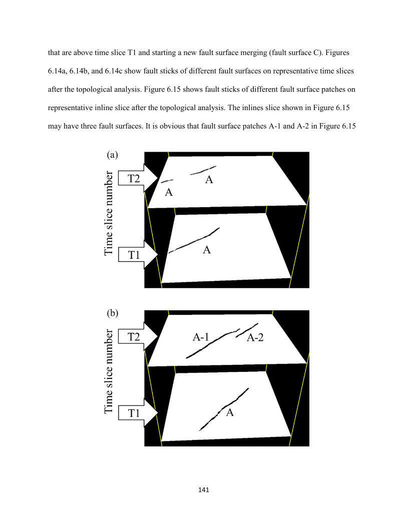
141

that are above time slice T1 and starting a new fault surface merging (fault surface C). Figures

6.14a, 6.14b, and 6.14c show fault sticks of different fault surfaces on representative time slices

after the topological analysis. Figure 6.15 shows fault sticks of different fault surface patches on

representative inline slice after the topological analysis. The inlines slice shown in Figure 6.15

may have three fault surfaces. It is obvious that fault surface patches A-1 and A-2 in Figure 6.15

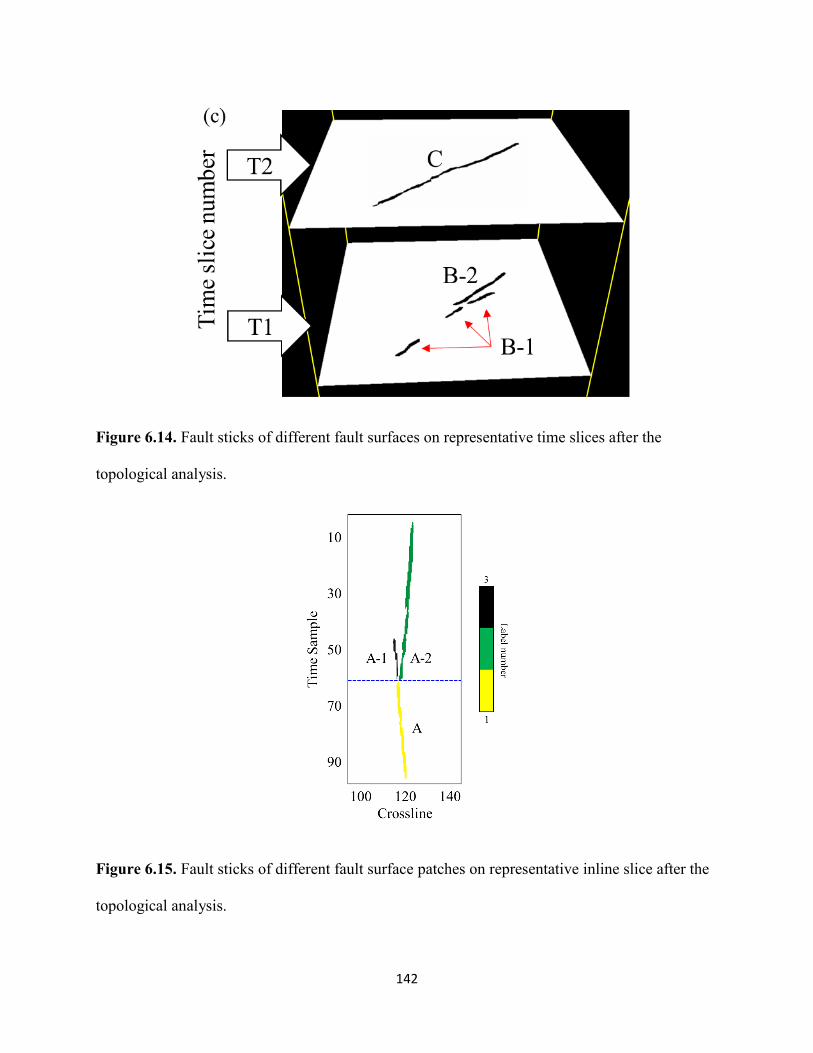
142

Figure 6.14. Fault sticks of different fault surfaces on representative time slices after the

topological analysis.

Figure 6.15. Fault sticks of different fault surface patches on representative inline slice after the

topological analysis.

143

belong to different fault surfaces. However, it is possible that fault surface patches A and A-1

belong to a same fault surface. Thus, we propose merging the fault surface patches by analyzing

the topological relationship between or among different fault surface patches.

Merging fault surface patches

We define three criteria for the merging of fault surface patches. The first criteria is that

the analyzed fault surface patch can only merge with its neighboring fault surface patches if it

shares vertical fault sticks with the analysis fault surface patch. Ideally, the fault surface patch

should not be allowed to merge any neighboring fault surface patches that have mutual exclusion

vertical sticks with the analysis fault surface patch. However, considering that the accuracy of

the input fault attribute, we allow the fault surface patch merging neighboring fault surface

patches if the percentage of exclusive fault sticks is below a user defined threshold smin (e.g., 5%

in this study). The third criteria is that the merging begins with the neighboring fault surface

patch that shares the most vertical fault sticks with analyzed fault surface patch. The analyzed

fault surface patch only merges one neighboring fault surface patch at a time and the merged

fault surface patch function as the new analyzed fault surface patch in the following merging.

The merging process continues until the algorithm cannot merge any two fault surface patches.

Figure 6.16 shows the automatically merged fault surface patches. The red, cyan, part of

blue (indicated by the red arrow in Figure 6.16), and yellow fault surface patches belong to the

same fault surface. The blue and green fault surface patches belong to other fault surfaces.

However, we must crop part of the blue fault surface patch indicated by the red arrow prior to the

merging between the blue and green fault surface patches. The inaccurate input fault attribute is

responsible for the inaccurate merging indicated by the red arrow in Figure 6.16. Figure 6.17

shows the fault sticks on representative time slices nearby the crossing time slices of two

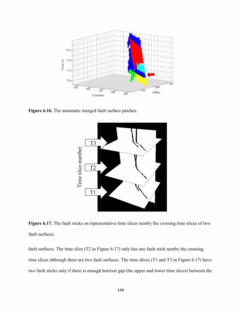
144

Figure 6.16. The automatic merged fault surface patches.

Figure 6.17. The fault sticks on representative time slices nearby the crossing time slices of two

fault surfaces.

fault surfaces. The time slice (T2 in Figure 6.17) only has one fault stick nearby the crossing

time slices although there are two fault surfaces. The time slices (T1 and T3 in Figure 6.17) have

two fault sticks only if there is enough horizon gap (the upper and lower time slices) between the

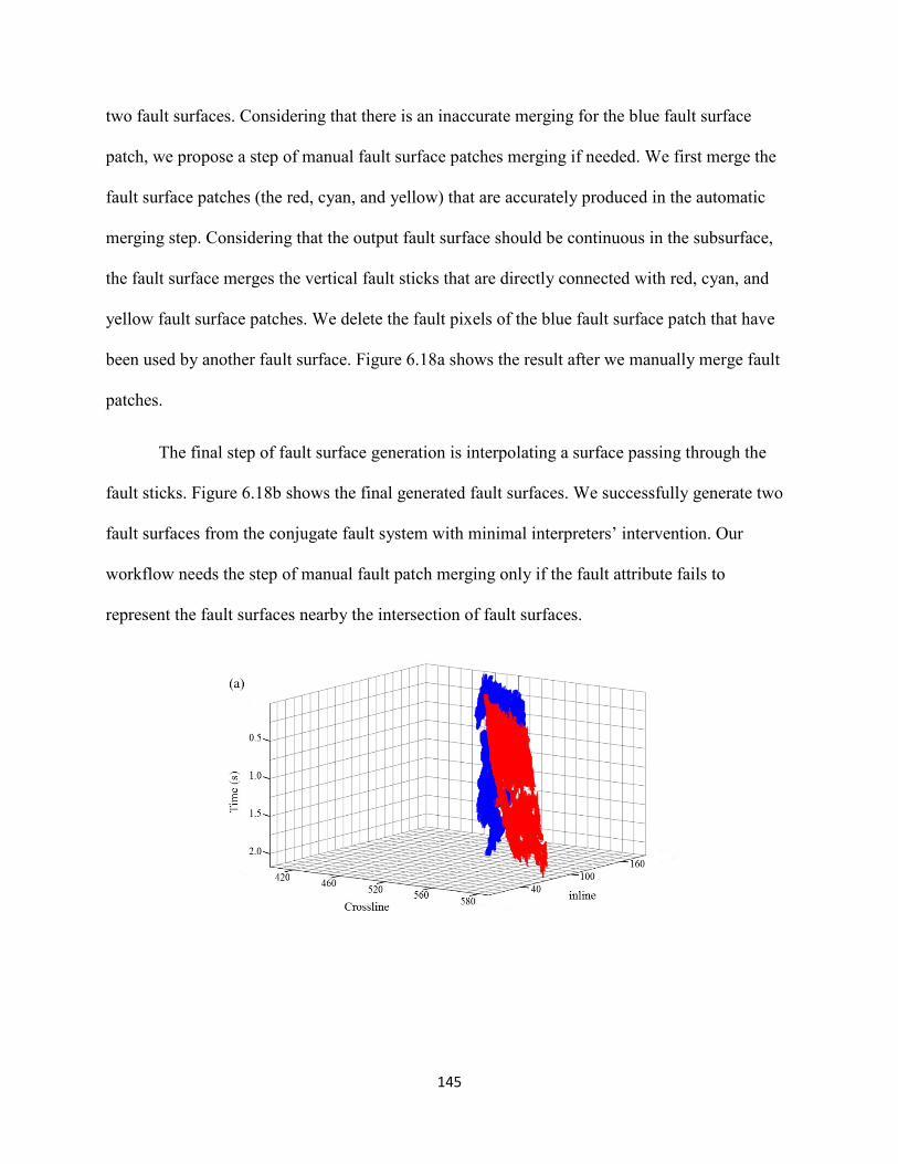
145

two fault surfaces. Considering that there is an inaccurate merging for the blue fault surface

patch, we propose a step of manual fault surface patches merging if needed. We first merge the

fault surface patches (the red, cyan, and yellow) that are accurately produced in the automatic

merging step. Considering that the output fault surface should be continuous in the subsurface,

the fault surface merges the vertical fault sticks that are directly connected with red, cyan, and

yellow fault surface patches. We delete the fault pixels of the blue fault surface patch that have

been used by another fault surface. Figure 6.18a shows the result after we manually merge fault

patches.

The final step of fault surface generation is interpolating a surface passing through the

fault sticks. Figure 6.18b shows the final generated fault surfaces. We successfully generate two

fault surfaces from the conjugate fault system with minimal interpreters’ intervention. Our

workflow needs the step of manual fault patch merging only if the fault attribute fails to

represent the fault surfaces nearby the intersection of fault surfaces.

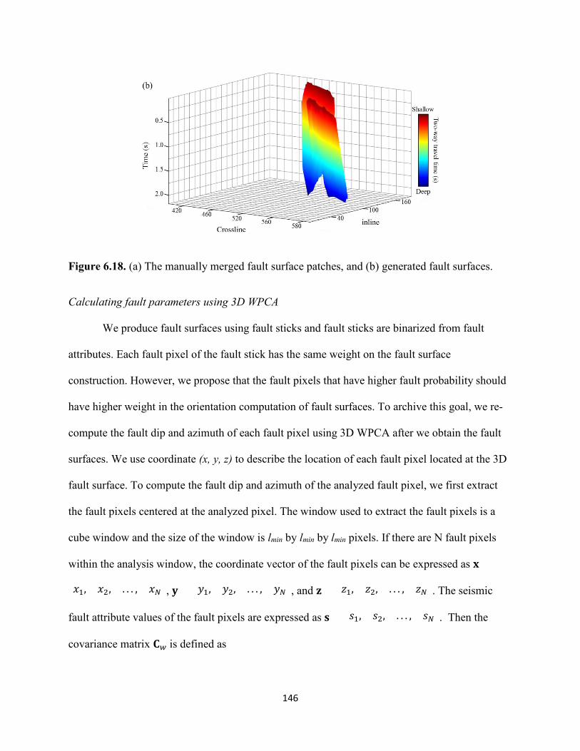
146

Figure 6.18. (a) The manually merged fault surface patches, and (b) generated fault surfaces.

Calculating fault parameters using 3D WPCA

We produce fault surfaces using fault sticks and fault sticks are binarized from fault

attributes. Each fault pixel of the fault stick has the same weight on the fault surface

construction. However, we propose that the fault pixels that have higher fault probability should

have higher weight in the orientation computation of fault surfaces. To archive this goal, we re-

compute the fault dip and azimuth of each fault pixel using 3D WPCA after we obtain the fault

surfaces. We use coordinate (x, y, z) to describe the location of each fault pixel located at the 3D

fault surface. To compute the fault dip and azimuth of the analyzed fault pixel, we first extract

the fault pixels centered at the analyzed pixel. The window used to extract the fault pixels is a

cube window and the size of the window is lmin by lmin by lmin pixels. If there are N fault pixels

within the analysis window, the coordinate vector of the fault pixels can be expressed as 𝐱𝐱 =

(𝑥𝑥1, 𝑥𝑥2, . . . , 𝑥𝑥𝑁𝑁), 𝐲𝐲 = (𝑦𝑦1, 𝑦𝑦2, . . . , 𝑦𝑦𝑁𝑁), and 𝐳𝐳 = (𝑧𝑧1, 𝑧𝑧2, . . . , 𝑧𝑧𝑁𝑁). The seismic

fault attribute values of the fault pixels are expressed as 𝐬𝐬 = (𝑠𝑠1, 𝑠𝑠2, . . . , 𝑠𝑠𝑁𝑁). Then the

covariance matrix 𝐂𝐂𝑖𝑖 is defined as

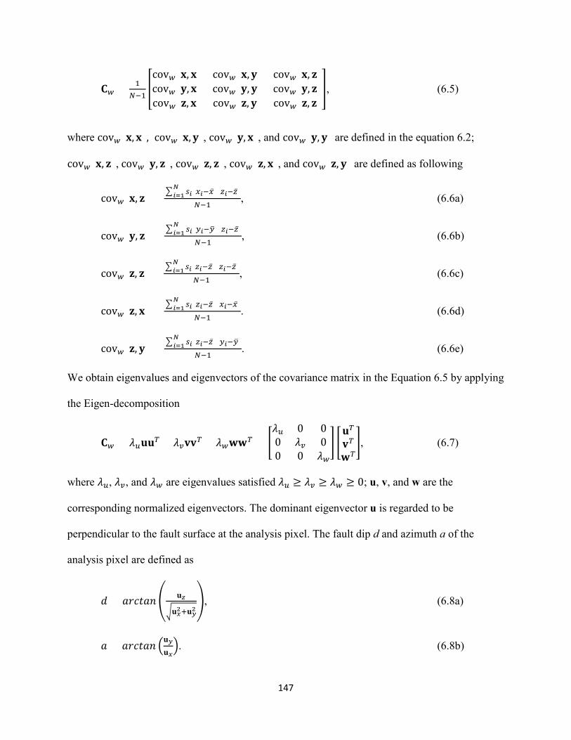
147

𝐂𝐂𝑖𝑖 = 1𝑁𝑁−1

�cov𝑖𝑖(𝐱𝐱, 𝐱𝐱) cov𝑖𝑖(𝐱𝐱,𝐲𝐲) cov𝑖𝑖(𝐱𝐱, 𝐳𝐳)cov𝑖𝑖(𝐲𝐲,𝐱𝐱) cov𝑖𝑖(𝐲𝐲, 𝐲𝐲) cov𝑖𝑖(𝐲𝐲, 𝐳𝐳)cov𝑖𝑖(𝐳𝐳, 𝐱𝐱) cov𝑖𝑖(𝐳𝐳, 𝐲𝐲) cov𝑖𝑖(𝐳𝐳, 𝐳𝐳)

�, (6.5)

where cov𝑖𝑖(𝐱𝐱,𝐱𝐱), cov𝑖𝑖(𝐱𝐱,𝐲𝐲), cov𝑖𝑖(𝐲𝐲, 𝐱𝐱), and cov𝑖𝑖(𝐲𝐲, 𝐲𝐲) are defined in the equation 6.2;

cov𝑖𝑖(𝐱𝐱, 𝐳𝐳), cov𝑖𝑖(𝐲𝐲, 𝐳𝐳), cov𝑖𝑖(𝐳𝐳, 𝐳𝐳), cov𝑖𝑖(𝐳𝐳, 𝐱𝐱), and cov𝑖𝑖(𝐳𝐳, 𝐲𝐲) are defined as following

cov𝑖𝑖(𝐱𝐱, 𝐳𝐳) =� 𝑠𝑠𝑖𝑖(𝑥𝑥𝑖𝑖−�̅�𝑥)𝑁𝑁

𝑖𝑖=1 (𝑧𝑧𝑖𝑖−�̅�𝑧)

𝑁𝑁−1, (6.6a)

cov𝑖𝑖(𝐲𝐲, 𝐳𝐳) =� 𝑠𝑠𝑖𝑖(𝑦𝑦𝑖𝑖−𝑦𝑦�)𝑁𝑁

𝑖𝑖=1 (𝑧𝑧𝑖𝑖−�̅�𝑧)

𝑁𝑁−1, (6.6b)

cov𝑖𝑖(𝐳𝐳, 𝐳𝐳) =� 𝑠𝑠𝑖𝑖(𝑧𝑧𝑖𝑖−�̅�𝑧)𝑁𝑁

𝑖𝑖=1 (𝑧𝑧𝑖𝑖−�̅�𝑧)

𝑁𝑁−1, (6.6c)

cov𝑖𝑖(𝐳𝐳, 𝐱𝐱) =� 𝑠𝑠𝑖𝑖(𝑧𝑧𝑖𝑖−�̅�𝑧)𝑁𝑁

𝑖𝑖=1 (𝑥𝑥𝑖𝑖−�̅�𝑥)

𝑁𝑁−1. (6.6d)

cov𝑖𝑖(𝐳𝐳, 𝐲𝐲) =� 𝑠𝑠𝑖𝑖(𝑧𝑧𝑖𝑖−�̅�𝑧)𝑁𝑁

𝑖𝑖=1 (𝑦𝑦𝑖𝑖−𝑦𝑦�)

𝑁𝑁−1. (6.6e)

We obtain eigenvalues and eigenvectors of the covariance matrix in the Equation 6.5 by applying

the Eigen-decomposition

𝐂𝐂𝑖𝑖 = 𝜆𝜆𝑢𝑢𝐮𝐮𝐮𝐮𝐼𝐼 + 𝜆𝜆𝑣𝑣𝐯𝐯𝐯𝐯𝐼𝐼 + 𝜆𝜆𝑖𝑖𝐰𝐰𝐰𝐰𝐼𝐼 = �𝜆𝜆𝑢𝑢 0 00 𝜆𝜆𝑣𝑣 00 0 𝜆𝜆𝑖𝑖

� �𝐮𝐮𝐼𝐼𝐯𝐯𝐼𝐼𝐰𝐰𝐼𝐼

�, (6.7)

where 𝜆𝜆𝑢𝑢, 𝜆𝜆𝑣𝑣, and 𝜆𝜆𝑖𝑖 are eigenvalues satisfied 𝜆𝜆𝑢𝑢 ≥ 𝜆𝜆𝑣𝑣 ≥ 𝜆𝜆𝑖𝑖 ≥ 0; u, v, and w are the

corresponding normalized eigenvectors. The dominant eigenvector u is regarded to be

perpendicular to the fault surface at the analysis pixel. The fault dip d and azimuth a of the

analysis pixel are defined as

𝑑𝑑 = 𝑎𝑎𝑎𝑎𝑎𝑎𝑡𝑡𝑎𝑎𝑛𝑛 � 𝐮𝐮𝑧𝑧

�𝐮𝐮𝑥𝑥2+𝐮𝐮𝑦𝑦2�, (6.8a)

𝑎𝑎 = 𝑎𝑎𝑎𝑎𝑎𝑎𝑡𝑡𝑎𝑎𝑛𝑛 �𝐮𝐮𝑦𝑦𝐮𝐮𝑥𝑥�. (6.8b)

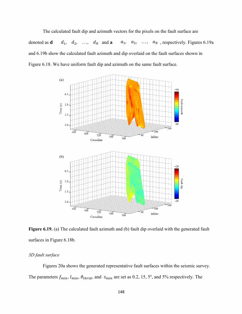
148

The calculated fault dip and azimuth vectors for the pixels on the fault surface are

denoted as 𝐝𝐝 = (𝑑𝑑1, 𝑑𝑑2, . . . , 𝑑𝑑𝑁𝑁) and 𝐚𝐚 = (𝑎𝑎1, 𝑎𝑎2, . . . , 𝑎𝑎𝑁𝑁), respectively. Figures 6.19a

and 6.19b show the calculated fault azimuth and dip overlaid on the fault surfaces shown in

Figure 6.18. We have uniform fault dip and azimuth on the same fault surface.

Figure 6.19. (a) The calculated fault azimuth and (b) fault dip overlaid with the generated fault

surfaces in Figure 6.18b.

3D fault surface

Figures 20a shows the generated representative fault surfaces within the seismic survey.

The parameters 𝑓𝑓𝑚𝑚𝑟𝑟𝑛𝑛, 𝑙𝑙𝑚𝑚𝑟𝑟𝑛𝑛, 𝜃𝜃𝑡𝑡ℎ𝑟𝑟𝑙𝑙𝑠𝑠, and 𝑠𝑠𝑚𝑚𝑟𝑟𝑛𝑛 are set as 0.2, 15, 5o, and 5% respectively. The

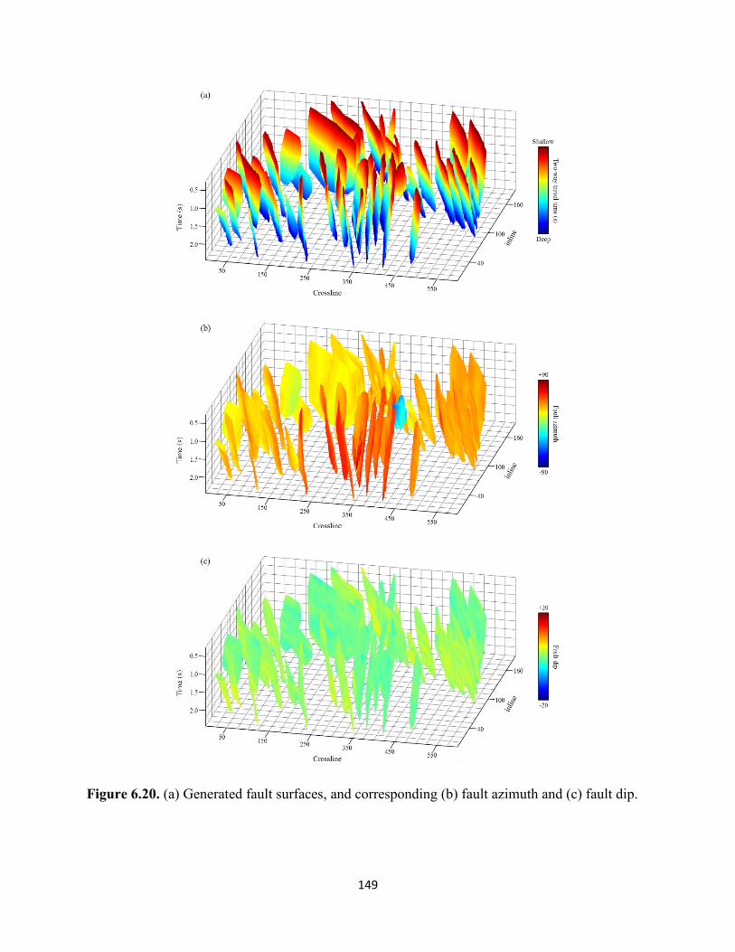
149

Figure 6.20. (a) Generated fault surfaces, and corresponding (b) fault azimuth and (c) fault dip.

150

value of 𝑙𝑙𝑚𝑚𝑟𝑟𝑛𝑛 is 15 which means our algorithm will not construct surfaces for those faults whose

largest thinned fault stick on time or vertical slices is less than 15 pixels. We generate 192 fault

surfaces in this seismic survey and Figure 20a only shows the biggest 60 fault surfaces. Figures

6.20b and 6.20c show the fault azimuth and dip overlaid with fault surfaces in Figures 6.20a,

respectively. We have uniform fault dip and azimuth on the same fault surface.

CONCLUSIONS

We proposed a novel workflow to automatically generate fault surfaces from seismic

fault attributes. It is a complex procedure of analyzing the topological relationship among the

fault pixels in a 3D manner. Our workflow is based on analyzing the topological relationship

(connectivity and mutual exclusion) among the fault sticks on time and vertical slices. The

quality of input seismic fault attribute is one of the key factors for successful implementing our

workflow. If the seismic fault attribute has strong staircase artifacts and undesired stratigraphic

anomalies, it is better to condition the seismic fault attributes prior to applying our workflow. In

our workflow, deep learning algorithms can produce high quality seismic fault attributes without

staircase artifacts.

The proposed workflow needs interpreters defining four parameters: (1) coherence

threshold 𝑓𝑓𝑚𝑚𝑟𝑟𝑛𝑛 used to generate fault sticks, (2) the smallest length 𝑙𝑙𝑚𝑚𝑟𝑟𝑛𝑛 in pixel of thinned fault

sticks we want to detect on time or vertical slices, (3) the orientation threshold 𝜃𝜃𝑡𝑡ℎ𝑟𝑟𝑙𝑙𝑠𝑠 used to

refine fault sticks, and (4) the percentage of exclusive fault sticks s_min used in step of the

surface patches merging. We suggest the coherence threshold 𝑓𝑓𝑚𝑚𝑟𝑟𝑛𝑛 to be set as a value between

0.2*𝑓𝑓𝑚𝑚𝑎𝑎𝑥𝑥 and 0.4*𝑓𝑓𝑚𝑚𝑎𝑎𝑥𝑥, where 𝑓𝑓𝑚𝑚𝑎𝑎𝑥𝑥 is the maximum value of fault probability. The smallest

length 𝑙𝑙𝑚𝑚𝑟𝑟𝑛𝑛 in pixel is determined by the smallest fault surface size we want to identify within

the seismic survey. Our workflow will ignore those fault surfaces whose largest fault stick size

151

on time or vertical slices is smaller than 𝑙𝑙𝑚𝑚𝑟𝑟𝑛𝑛. Note the size of one pixel along vertical axis is the

same length of time sample interval. Similarly, the sizes of one pixel along inline and crossline

are the same length of seismic trace interval along inline and crossline, respectively. A small

value of threshold 𝜃𝜃𝑡𝑡ℎ𝑟𝑟𝑙𝑙𝑠𝑠 reduces the time of generating fault surfaces but increases the time of

merging fault surfaces. Considering that we have an optional step of manual merging, we suggest

using a small value of threshold 𝜃𝜃𝑡𝑡ℎ𝑟𝑟𝑙𝑙𝑠𝑠 and a small value can guarantee the accuracy of generated

fault surface patches. The percentage threshold 𝑠𝑠𝑚𝑚𝑟𝑟𝑛𝑛 is determined by the quality of input fault

attribute. We find that it is much easier merging fault surface patches than separating wrongly

merged fault surface patches. Thus, we suggest to set a relative low value (e.g., smaller than

10%) to 𝑠𝑠𝑚𝑚𝑟𝑟𝑛𝑛. Of course, we need interpreters to testing those parameters case by case.

152

REFERENCES

AlBinHassan, N. and K. Marfurt, 2003, Fault detection using Hough transforms: SEG Technical Program Expanded Abstracts 2003, 1719-1721.

Al-Dossary, S., and K. J. Marfurt, 2006, 3D volumetric multispectral estimates of reflector curvature and rotation: Geophysics, 71(5), P41–P51.

Aqrawi, A. A., and T. H. Boe, 2011, Improved fault segmentation using a dip guided and modified 3D Sobel filter: SEG Technical Program Expanded Abstracts 2011, 999-1003.

Bakker, P., L. J. van Vliet, and P.W. Verbeek, 1999, Edge-preserving orientation adaptive filtering: Proceedings, 1999 IEEE Computer Society Conference on Computer Vision and Pattern Recognition, 1, 535-540.

Cohen, I., N. Coult, and A. A. Vassiliou, 2006, Detection and extraction of fault surfaces in 3D seismic data: Geophysics, 71(4), P21–P27.

Di, H., and D. Gao, 2016, Efficient volumetric extraction of most positive/negative curvature and flexure for fracture characterization from 3D seismic data: Geophysical Prospecting, 64, 1454–1468.

Fan, Z., E. Liu, and B. Xu, 2011, Weighted principal component analysis: International Conference on Artificial Intelligence and Computational Intelligence, 569-574.

Fehmers, G. C., and C. F. Höcker, 2003, Fast structural interpretation with structure-oriented filtering: Geophysics, 68(4), 1286-1293.

Gersztenkorn, A., and K. J. Marfurt, 1999, Eigenstructure based coherence computations as an aid to 3D structural and stratigraphic mapping: Geophysics, 64(5), 1468–1479.

Hale, D., 2009, Structure-oriented smoothing and semblance: CWP Report, 635, 261-270.

Hale, D., 2013, Methods to compute fault images, extract fault surfaces, and estimate fault throws from 3D seismic images: Geophysics, 78(2), O33–O43.

Lou, Y., B. Zhang, R. Wang, T. Lin, and D. Cao, 2019, Seismic Fault Attribute Estimation Using a Local Fault Model: Geophysics, 84(4), O73-O80.

Luo, Y., M. Marhoon, S. Al-Dossary, and M. Alfaraj, 2002, Edge-preserving smoothing and applications: The Leading Edge, 21(2), 136–158.

Luo, Y., W. G. Higgs, and W. S. Kowalik, 1996, Edge detection and stratigraphic analysis using 3D seismic data: SEG Technical Program Expanded Abstracts 1996, 324-327.

Marfurt, K. J., 2006, Robust estimates of 3D reflector dip and azimuth: Geophysics, 71(4), P29-P40.

153

Marfurt, K. J., R. L. Kirlin, S. H. Farmer, and M. S. Bahorich, 1998, 3D seismic attributes using a running window semblance-based algorithm: Geophysics, 63(4), 1150-1165.

Neff, D. B., J. R. Grismore, and W. A. Lucas, 2000, Automated seismic fault detection and picking: U.S. Patent, 6,018,498.

Pedersen, S. I., T. Randen, L. Sonneland, and Ø. Steen, 2002, SEG Technical Program Expanded Abstracts 2002, 512–515.

Pedersen, S. I., T. Skov, A. Hetlelid, P. Fayemendy, T. Randen, and L. Sønneland, 2003, New paradigm of fault interpretation: SEG Technical Program Expanded Abstracts 2003, 350–353.

Qi, J., B. Lyu, A. AlAli, G. Machado, Y. Hu, and K. J. Marfurt, 2018, Image processing of seismic attributes for automatic fault extraction: Geophysics, 84(1), O25-O37.

Qi, J., F. Li, and K. J. Marfurt, 2017a, Multiazimuth coherence: Geophysics, 82(6), O83-O89.

Qi, J. and J. Castagna, 2013, Application of a PCA fault-attribute and spectral decomposition in Barnett Shale fault detection: SEG Technical Program Expanded Abstracts 2013, 1421-1425.

Qi, J., G. Machado, and K. J. Marfurt, 2017b, A workflow to skeletonize faults and stratigraphic features: Geophysics, 82(4), O57–O70.

Wu, X., 2017, Directional structure-tensor based coherence to detect seismic channels and faults: Geophysics, 82(2), A13-A17.

Wu, X. and D. Hale, 2016, 3D seismic image processing for faults: Geophysics, 81(2), IM1-IM11.

Wu, X., and S. Fomel, 2018, Automatic fault interpretation with optimal surface voting: Geophysics, 83(5), O67–O82.

Zhang, B., Y. Liu, M. Pelissier, and N. Hemstra, 2014, Semiautomated fault interpretation based on seismic attributes: Interpretation, 2(1), SA11–SA19.

154

CHAPTER 7 CONCLUSION

In this dissertation, I have developed new algorithms and workflows to accelerate the

procedure of seismic horizon and fault interpretations. I develop an algorithm to generate an

accurate seismic reflector dip attribute, and propose a workflow to automatically interpret

horizon surfaces from a 3D seismic survey using the new seismic dip attribute. I finally propose

a workflow to automatically generate control points for horizon tracking, and construct seismic

horizons by using generated control points. I develop an algorithm to generate a new fault

attribute, and propose a workflow to automatically interpret fault surfaces from 3D seismic

survey using the new fault attribute. The main conclusions of this dissertation are summarized as

follows.

In Chapter 2, I propose a new algorithm to improve the accuracy of volumetric dip

estimation by combing and improving the multiple window scanning method and GST analysis.

The proposed algorithm first obtains an estimated rough dip and azimuth for local seismic

reflectors using the semblance scanning method. The algorithm next generates the analysis

window, which is “roughly” parallel with the local seismic reflectors using the estimated “rough”

dip and azimuth. The algorithm then estimates the dip and azimuth of the local seismic reflectors

within the analysis window using GST analysis. To improve the robustness of GST analysis, the

proposed algorithm employs analytic seismic traces to compute the GST matrix. The algorithm

finally determines the dip and azimuth of local seismic reflectors by employing the Kuwahara

window searching strategy. Our proposed algorithm precisely estimates reflectors dip near steep

155

structures. The seismic reflector dip estimated using the proposed algorithm has better anti-noise

performance.

In Chapter 3, I propose a new workflow to automatically generate seismic horizons using

multiple seismic attributes and generate a relative geological time (RGT) volume. The proposed

workflow assumes that seismic horizons follow local seismic reflector dip, and the same horizon

should have similar instantaneous phase values. The horizon tracking workflow begins with

generating horizon patches using seismic reflector dip attributes. The tracked horizon patches

stop at potential faults or unconformities by considering the coherence of samples. Considering

the inaccuracy of reflector dip near the discontinuous structures, the workflow next refines the

generated horizon patches using instantaneous phase. The final step is to iteratively merge

different horizon patches into single horizons throughout the seismic survey, and build the

corresponding RGT volume. The proposed automatic horizon tracking workflow is capable of

generating a horizon for each reflection within the 3D seismic survey. Each sample of the

seismic survey is assigned a chronostratigraphic relative geologic time value according to the

tracked horizons.

In Chapter 4, I propose a new workflow to automatically generate seismic horizons by

simulating the procedure of manual seismic horizon picking. The proposed workflow

automatically tracks horizons on inline and crossline independently, and evaluates the tracked

horizons using the defined loop-tie checking, which is similar with the loop-tie checking in

manual horizon picking. To simulate the loop-tie checking in manual horizon picking, I define

two dip attributes for each time sample of seismic traces: “left” and “right” reflector dips. The

proposed workflow only preserves the portion of tracked horizon, which meets the defined loop-

tie checking. The next step is to merge tracked horizons and the two-way travel time of merged

156

horizons function as the hard controls for the horizon surface generating step. The final step is to

use the seismic dip attribute to track the horizon surfaces over the seismic survey under the hard

controls. The proposed workflow can extract accurate horizons near the discontinuity locations

such as faults and unconformity zones.

In Chapter 5, I propose a novel algorithm to generate a new fault attribute without the

staircase artifacts and undesired stratigraphic anomalies using a local fault model. The proposed

algorithm assumes that each sample of the seismic data is located at a potential fault plane. The

hypothesized fault divides the seismic data centered at the analysis sample into two sub-

windows. The proposed algorithm computes the coherence for the two sub-windows and for the

full analysis window. The algorithm then repeats the coherence computation step by rotating the

hypothesized fault plane along a set of user-defined discrete fault dip and azimuth. If the analysis

point is not located at a fault plane, the calculated coherence values for the sub-windows and full

window should be almost same. However, if the analysis point is located at a fault plane, the

calculated coherence should be varied with user-defined discrete fault dip and azimuth. The

“best” fault plane results in maximum coherence for the sub-windows and minimum coherence

for the full window. Therefore, I determine the fault probability, fault dip, and fault azimuth by

analyzing the computed coherence of the two sub-windows and the full window. To improve the

continuity of the fault attributes, we finally smooth the fault probability attribute along the

estimated fault plane. Our proposed algorithm successfully minimizes staircase artifacts and

stratigraphic anomalies and generates more continuous fault attribute.

In Chapter 6, I propose a new workflow to automatically construct seismic fault surfaces

through the topology analysis of seismic fault attributes. The proposed workflow consists of

three steps and is based on analyzing the features of fault attributes on 2D slices. The first step of

157

the fault surface construction workflow is generating fault sticks using seismic fault attribute.

The fault stick generation algorithm begins with generating initial fault sticks on 2D vertical and

horizontal slices. The algorithm then computes the orientation of initial fault sticks by integrating

the Kuwahara window searching method and the weighted principal component analysis

(WPCA). The algorithm finally obtains refined fault sticks by analyzing the orientation of the

initial fault sticks. The second step of the proposed fault surface construction workflow is

grouping fault sticks by analyzing the topological relationships between the faults sticks on

vertical and horizontal slices. The third step of the proposed workflow is generating fault surface

patches by merging the fault sticks time slice by time slice through the topology analysis. The

proposed workflow allows users to manually merging the fault patches if needed. The proposed

fault surface construction workflow is capable of generating fault surfaces for all the faults

including conjugate faults contained in the seismic data. The workflow can also compute the

fault parameters such as fault dip and strike using 3D WPCA.