1

Date of preparation: 22 July 2004

Running head: Separation of NEE

Title: On the separation of net ecosystem exchange into assimilation and

ecosystem respiration: review and improved algorithm

Authors: Markus Reichstein1), Eva Falge2), Dennis Baldocchi3), Dario Papale1),

Riccardo Valentini1), Marc Aubinet4), Paul Berbigier5), Christian Bernhofer6), Nina

Buchmann7),8), Tagir Gilmanov9), André Granier10), Thomas Grünwald6), Katka

Havránková11), Daniel Janous11), Alexander Knohl7,3), Tuomas Laurela12), Annalea

Lohila12), Denis Loustau13), Giorgio Matteucci14), Tilden Meyers15), Franco Miglietta16),

Jean-Marc Ourcival17), Serge Rambal17), Eyal Rotenberg18), Maria Sanz19), John

Tenhunen20), Günther Seufert14), Francesco Vaccari16), Timo Vesala21), Dan Yakir18)

1) Dept. of Forest Science and Environment, University of Tuscia, 01100 Viterbo, Italy

2) Department of Plant Ecology, University of Bayreuth, D-95440 Bayreuth 3) University of California, Department of Environmental Science, Policy and Management, Ecosystem Science Division, 151 Hilgard Hall #3110, Berkeley, CA 94720-3110, USA 4) Unité de Physique, Faculté des Sciences Agronomiques de Gembloux, B-50 30 Gembloux, Belgium 5) INRA, Bioclimatologie, Bordeaux, France 6) Technische Universität Dresden, IHM - Meteorologie, Pienner Strasse 9, 01737 Tharandt 7) Max Planck Institute for Biogeochemistry, PO Box 100164, 07701 Jena, Germany 8) Institute of Plant Science, ETH Zürich, Universitätsstrasse 2, 8092 Zürich, Switzerland 9) Dept. of Biology/Microbiology AgH 310, Box 2207B South Dakota State University Brookings, SD 57007-2142 10) INRA, Unité d’Ecophysiologie Forestière, F-54280 Champenoux, France 11) Laboratory of Ecological Physiology of Forest Trees, Institute of Landscape Ecology, Academy of Sciences of the Czech Republic, Porici 3B, Brno 603 00, Czech Republic 12) Finnish Meteorological Institute, Sahaajankatu 20 E, 00880 Helsinki, Finland 13) INRA - Ecophysiologie, Domaine de l'Hermitage - Pierroton, 69, route d'Arcachon, 33610 Cestas, France 14) JRC, Institute for Environment and Sustainability, Via Enrico Fermi, T.P. 051, 21020 Ispra (VA), Italy 15) NOAA/Atmospheric Turbulence and Diffusion,: PO Box 2456 Oak Ridge, TN 37830 16) IBIMET, P.le delle Cascine, 18, 50144 Firenze, Italy 17) DREAM Unit, Centre d’Ecologie Fonctionelle et Evolutive, CNRS, 1919 route de Mende, Montpellier, France 18) Dept. of Environmental Sciences and Energy Research, Weizmann Institute of Science, P.O. Box 26, Rehovot 76100, Israel 19) CEAM, Parque Tecnológico, c/Charles H. Darwin 14, 46980 Paterna (Valencia), Spain 20) Department of Plant Ecology, University of Bayreuth, D-95440 Bayreuth, Germany 21) Department of Physical Sciences, FIN-00014 University of Helsinki, Finland

Keywords: carbon balance, eddy covariance, gross carbon uptake, ecosystem respiration, computational methods, temperature sensitivity of respiration

Corresponding author: Markus Reichstein, Dept. of Forest Science and Environment,

University of Tuscia, 01100 Viterbo, Italy, e-mail: reichstein@unitus.it, FAX:

+39.0761.357389

2

FFECTS ON ECOSYSTEM RESPIRATION

On the separation of net ecosystem exchange into

assimilation and ecosystem respiration: review and

improved algorithm

Abstract

This paper discusses the advantages and disadvantages of different methods to separate the

net ecosystem exchange (NEE) into its major components, gross ecosystem carbon uptake

(GEP) and ecosystem respiration (Reco). In particular we analyse the effect of the

extrapolation of night-time values of ecosystem respiration into the daytime; this is usually

done with a temperature response function that is derived from long-term data sets. For this

analysis we used 16 year-long data sets of carbon dioxide exchange measurements from

European and US-American eddy covariance network sites. These sites span from the boreal

to Mediterranean climate, and include deciduous and evergreen forest, scrubland and crop

ecosystems.

We show, that the temperature sensitivity of Reco, derived from long-term (annual) data

sets, does not reflect the short-term temperature sensitivity that is effective when extrapolating

from night-time to day-time. Specifically, in summer active ecosystems the long-term

temperature sensitivity exceeds the short-term sensitivity. Thus, in those ecosystems, the

application of a long-term temperature sensitivity to the extrapolation from night to day leads

to a systematic overestimation of ecosystem respiration at half-hourly to annual time-scales,

that can reach >25% for an annual budget and that consequently also affects estimates of

GEP.

We introduce a new generic algorithm that derives a short-term temperature sensitivity of

Reco from the eddy covariance data and applies this to the extrapolation from night- to day-

time, and further performs a gap-filling that exploits both, the covariance between fluxes and

3

meteorological drivers and the temporal auto-correlation of the fluxes. While this algorithm

should give less biased estimates of GEP and Reco, we discuss the remaining biases and

recommend that eddy covariance measurements are still backed by ancillary flux

measurements (e.g. chambers) that can reduce the uncertainties inherent in the eddy

covariance data.

Introduction

The eddy covariance method has become the main method for sampling ecosystem carbon,

water and energy fluxes from hourly to inter-annual time scales (Baldocchi et al., 2001) and

now serves as a backbone for bottom-up estimates of continental carbon balance components

(Papale and Valentini, 2002; Reichstein et al., 2003). Furthermore, eddy covariance data is

increasingly used for model calibration and validation (e.g., Baldocchi, 1997; Law et al.,

2001; Hanan et al., 2002; Reichstein et al., 2002; Reichstein et al., 2003). In the latter context

it is useful to separate or partition the directly observed net ecosystem exchange (NEE)

through a ‘flux-partitioning algorithm’ into gross ecosystem production (GEP) and ecosystem

respiration (Reco), since this provides a better diagnostic about which processes (assimilatory

or respiratory) are misrepresented in the model (Falge et al., 2002; Reichstein et al., 2002).

For instance, if a model overestimates both Reco and GEP by a similar amount, this model

error would not be detected via comparison of NEE that is the difference between Reco and

GPP. Furthermore, partitioning of the NEE flux is needed to better understand how inter-

annual and between-site variability of NEE is caused (Valentini et al., 2000). Apart from the

flux-partitioning, for sampling long-term budgets it is necessary to fill data gaps that occur

under unfavourable meteorological conditions (e.g., stability) and during instrument failure

(‘gap-filling’). While the gap-filling essentially is an interpolation of data and has received a

lot of systematic attention (Falge et al., 2001; Falge et al., 2001; Hui et al., 2003), most flux-

partitioning methods are an extrapolation of data from night-time to day-time and have only

been compared in a less systematic manner (Falge et al., 2002). In particular, one problem has

4

not received the necessary attention: For the extrapolation of night-time ecosystem respiration

data usually a temperature dependency is used that is derived from an annual data set.

However, it is expected that the seasonal apparent temperature sensitivity does not reflect the

actual short-term (hour-to-hour) temperature sensitivity, since the former is confounded by

other factors that co-vary with temperature, e.g. soil moisture, growth effects, rain pulses and

decomposition dynamics (e.g., Davidson et al., 1998; Reichstein et al., 2002; Xu and

Baldocchi, 2004). For instance, in a summer-active ecosystem like a summer-green deciduous

forest or a summer crop field, the apparent seasonal temperature sensitivity should be higher

than the short-term temperature sensitivity, since the high respiration fluxes in summer are

caused not only by high temperature but also by higher overall activity (leaves and fine-roots

are present and active, growth is occurring etc.). The opposite would be hypothesised for

(relative) summer-passive like Mediterranean ecosystems. Any systematic error in the

temperature sensitivity introduces a systematic error in the day-time estimate of Reco and

consequently GEP, and hence in annual sums of these quantities.

Thus, the objective of this paper is to review and discuss existing flux-partitioning

algorithms, and then to analyse the effect of short-term versus long-term temperature

sensitivity on the estimation of day-time Reco and thus GEP.

Short review of statistical methods for separation of NEE into assimilation and

ecosystem respiration

The final goal of any eddy covariance NEE flux partitioning algorithm is to estimate

ecosystem respiration (Reco) and gross carbon uptake (GEP) from the net ecosystem exchange

(NEE) according to the definition equation NEE=Reco-GEP. These flux-partitioning

algorithms can be classified in those that use only (filtered) night-time data for the estimation

of ecosystem respiration and those that exploit day-time data or both, day- and night-time data

using light-response curves (Table 1). These two general approaches have been compared by

5

(Falge et al., 2002) resulting in generally good agreement between the two methods,

obviously except in ecosystems where large carbon pools in the soil exist. Under those

conditions the light-curves derived from day-time data may not represent well respiratory

processes during night-time. Moreover, regressions of light-response curves sometimes tend

to yield unstable parameters (Falge, unpublished). While the standard light-response curve

method only allows the estimation of the daily average respiration without estimation of a

temperature dependent diurnal course, (Gilmanov et al., 2003) have developed a regression

model, where GEP and Reco are described in one equation, and where Reco is explicitly

dependent on air or soil temperature. Once regression parameters are fitted, GEP and Reco can

be computed separately on a half-hourly time step. While this is an elegant approach, if

suffers from three problems: 1) the estimation of the temperature response of Reco is

confounded by the response of GEP to VPD which can lead to a bias in the estimation of Reco.

Clearly, if an afternoon drop of NEE can be caused by a VPD related drop of GEP or by a

temperature related increase in Reco. If a regression model only ascribes the effect of Reco to

the drop of NEE, this consequently leads to an overestimation of Reco. 2) With this method,

both Reco and GEP are modelled and based on certain assumptions (e.g. hyperbolic light

response of GEP). If the flux-partitioned data is then used to evaluate models, one is

essentially comparing two models, which can lead to circular arguments (e.g. a model with

the same hyperbolic assumption will be more likely validated than other models). 3) CO2

fluxes near sunrise and sunset are very transient, involve instationarity problems and often

storage occurs. Problem 1) can be tackled by including a VPD response of GEP into the

regression model, but this might already lead to an overparameterized model. Problem 2) is

quite fundamental and virtually excludes using this method when the aim of the flux-

partitioning is model evaluation. Problem 3) is handled by accounting for storage it is only

measured imperfectly (e.g. if storage and turbulent fluxes have different source areas).

6

Maybe this is the reason why in most studies the flux-partitioning starts with the estimation

of Reco from night-time data (Hollinger et al., 1998; Law et al., 1999; Janssens et al., 2001;

Falge et al., 2002; Reichstein et al., 2002; Reichstein et al., 2002; Rambal et al., 2003). As

shown in Table 1, these methods mainly differ in the way how Reco is modelled (apart from

the diversity of methods to determine the valid night-time fluxes, which is not the scope of

this paper, (Foken and Wichura, 1996; Aubinet et al., 2000). The simplest algorithm

represents Reco as one single function of temperature for the whole year, which is acceptable

only in a few – if in any – ecosystems, since usually other factors influence the rate of

respiration at a reference temperature (Rref). This effect of other factors has either been

incorporated explicitly by assimilation of the relevant factors into the function or implicitly by

introducing temporally varying functions of temperature, where Rref can vary with time. In

all cases, however, the temperature sensitivity of Reco has been kept constant over the year and

has been derived from relatively long data series that potentially introduce confounding

seasonal effects into the temperature response of Reco. The estimation of a correct temperature

sensitivity of Reco is crucial since Reco is extrapolated from night-time to day-time and any

under- or overestimation of the temperature sensitivity will lead to an over- or

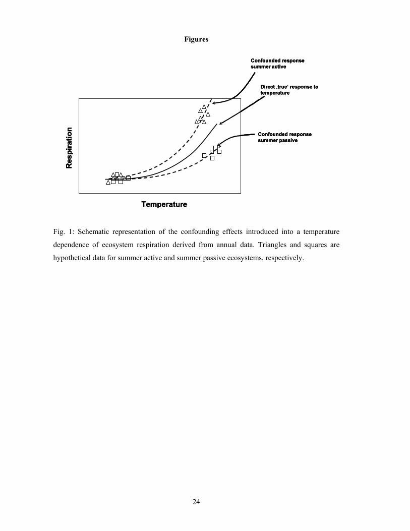
underestimation of day-time Reco, respectively (cf. Fig. 1). In the current study we develop a

flux-partitioning algorithm that first estimates the temperature sensitivity from short-term

periods, and then applies this short-term temperature sensitivity to extrapolate the ecosystem

respiration from night to day-time. In this case one can introduce a seasonally varying

temperature sensitivity or apply a site-specific constant temperature sensitivity (Table 1).

Methods

Eddy covariance data

The starting point of this analysis are half-hourly eddy covariance CO2 fluxes from sites

and vegetation types listed in Table 2, that are mainly European boreal to Mediterranean

forest, shrubland and crop sites. To allow for a better representation of crop sites two US-

7

American crop flux data sets from soybean and corn fields have been added. Only original

data (not gap-filled) was used in this analysis, and all night-time data with non-turbulent

conditions were dismissed based on a u*-threshold criterion (Aubinet et al., 2000). The u*-

threshold was derived specifically for each site as in Reichstein et al. (2002). Night-time data

was selected according to a global radiation threshold of 20 W m-2 (night below that

threshold), cross-checked against sunrise and sunset data derived from the local time and

standard sun-geometrical routines, and defined as ecosystem respiration (Reco).

Estimation of temperature sensitivity from seasonal data

For the estimation of the temperature sensitivity from seasonal data, all the available

ecosystem respiration data are simply related to temperature using the exponential regression

model (Lloyd and Taylor, 1994):

−−

−⋅

⋅= 00,0

11TTTT

E

refecorefeRR

long

Eq. 1

While the regression parameter T0 is kept constant at –46.02°C as in Lloyd and Taylor

(1994), the activation energy kind of parameter (E0), that essentially determines the

temperature sensitivity is a free parameter. The reference temperature (Tref) is set to 10°C as

in the original model.

Estimation of temperature sensitivity from short-term data

For this estimation the data set is divided into windows of 15 days, where window x+1 is

shifted 5 days with respect to window x (i.e. 10 days overlap). For each period it is checked

whether more than six data points are available and whether the temperature range is more

than 5°C, since only under these conditions reasonable regressions of Reco versus temperature

are expected. For each of those periods where the criteria were met, the Lloyd-and-Taylor

(1994) regression model

8

−−

−⋅

⋅= 00,0

11TTTT

E

refecorefeRR

short

Eq. 2

was fitted to the scatter of ecosystem respiration (Reco) versus either soil or air temperature

(T). While the regression parameter T0 was kept constant at –46.02°C as in Lloyd and Taylor

(1994), the activation energy kind of parameter (E0), that essentially determines the

temperature sensitivity was allowed to vary. The reference temperature was set to 10°C as in

the original model. Since not all at sites soil temperatures were available, soil temperatures

were measured at different depth and often more variance of ecosystem respiration was

explained by air temperature we show here results obtained using air temperature. [This result

is rather empirical and does not imply a mechanistic interpretation that air temperature is the

main driver for ecosystem respiration. It may reflect that measurements of soil temperatures at

5-10 cm depth are already too deep since a lot of respiration evolves from surface soil

compartments, e.g. litter].

For each period, the regression parameters and statistics are kept in memory and evaluated

after regressions for all periods have been performed. Only those periods where the relative

standard error of the estimates of the parameter E0 is less than 50% and where estimates are

within realistic bounds are accepted. The E0 estimates from those three periods that yielded

the lowest standard errors are averaged constituting the best estimate of the short-term

temperature sensitivity of Reco that can be obtained from the data and is used for the whole

data set.

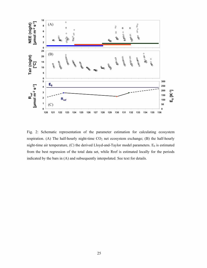
Estimation of day-and-night time ecosystem respiration

After the temperature sensitivities have been estimated, the overall level of respiration, i.e.

the Rref parameter, has to be estimated. Since this parameter is definitely temporally varying

in an ecosystem, it was estimated for consecutive four-day periods by non-linear regression

9

using the Lloyd-and-Taylor (1994) model, fixing all parameters except Rref. This estimation

was performed once using the long-term temperature sensitivity (E0,long) and once using the

short-term temperature sensitivity (E0,short). The Rref estimates were assigned to that point in

time, which represents the “center of gravity” of the data, for instance if only Reco data was

available during the fourth night of the period from 6 pm to 6 am, the Rref is assigned to

12pm of the fourth night. After the Rref parameters were estimated for each period, they were

linearly interpolated between the estimates (cf. Fig. 2). This procedure results in a dense

timeseries of the Lloyd-and-Taylor (1994) parameters Rref and E0, the latter being constant.

Consequently for each point in time an estimate of Reco can be provided according to

( ) ( ) ( )

−−

−⋅

⋅= 000

11TtTTT

E

refecosoilrefetRtR

Eq. 2

that is the same as Eq. 1, but with time-dependent parameters and variables indicated by

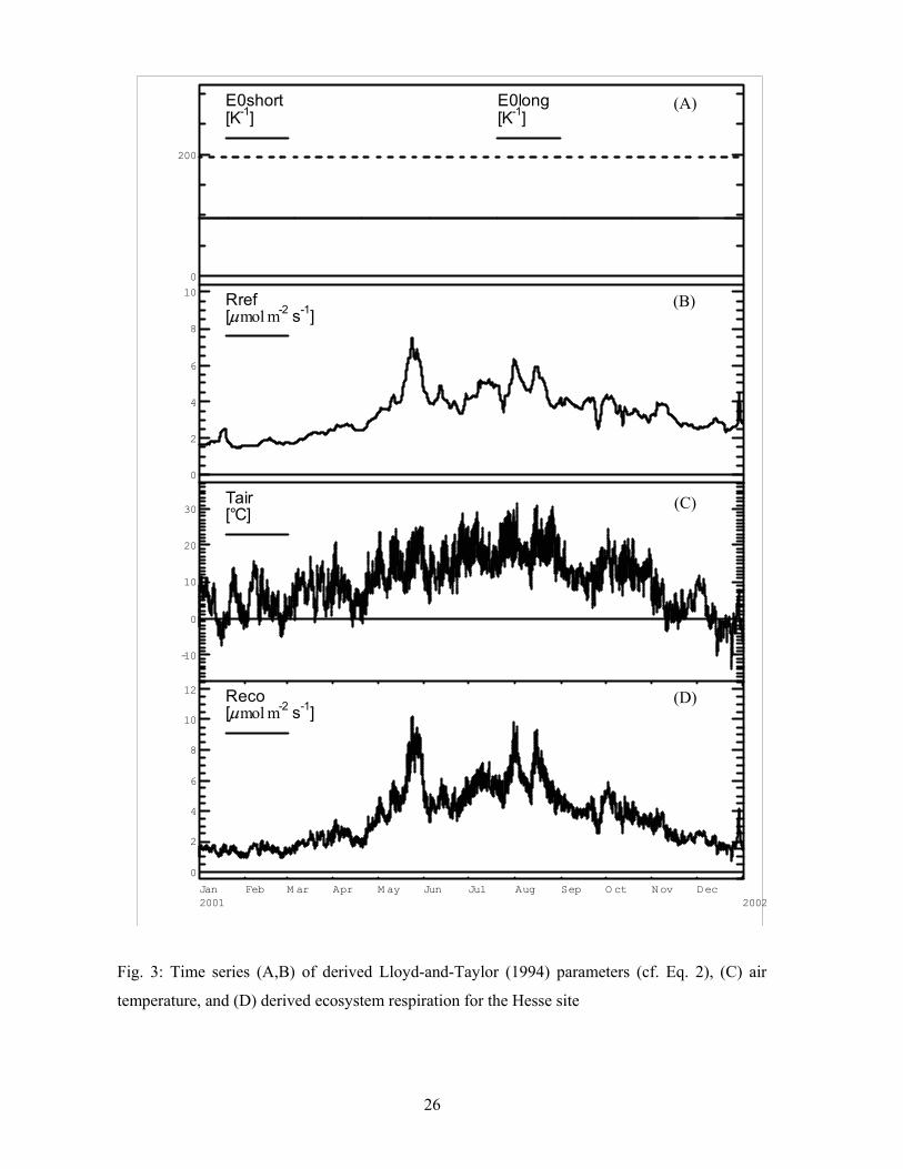
the symbol t in parenthesis. Examples of the time-course for those quantities in Eq. 2 are

shown in Fig. 3 for the Hesse beech forest site. Depending on whether E0 (and derived Rref)

from the long-term or short-term estimate is placed into the equation, Reco represents an

estimate of ecosystem respiration using the long-term or short-term sensitivity of respiration.

Gap-filling

The data was gap-filled using a combination and an enhancement of the Falge et al. (2001)

methods as described in the appendix.

Results and Discussion

As exemplified graphically for the Hesse site the (temperature independent) rate of

ecosystem respiration at reference conditions (Rref), varies seasonally more than three-fold

(Fig. 3b). Such seasonal changes have been often found earlier for soil respiration (e.g.

Davidson et al., 1998; Law et al., 1999; Law et al., 2001; Xu and Qi 2001; Subke et al., 2003)

10

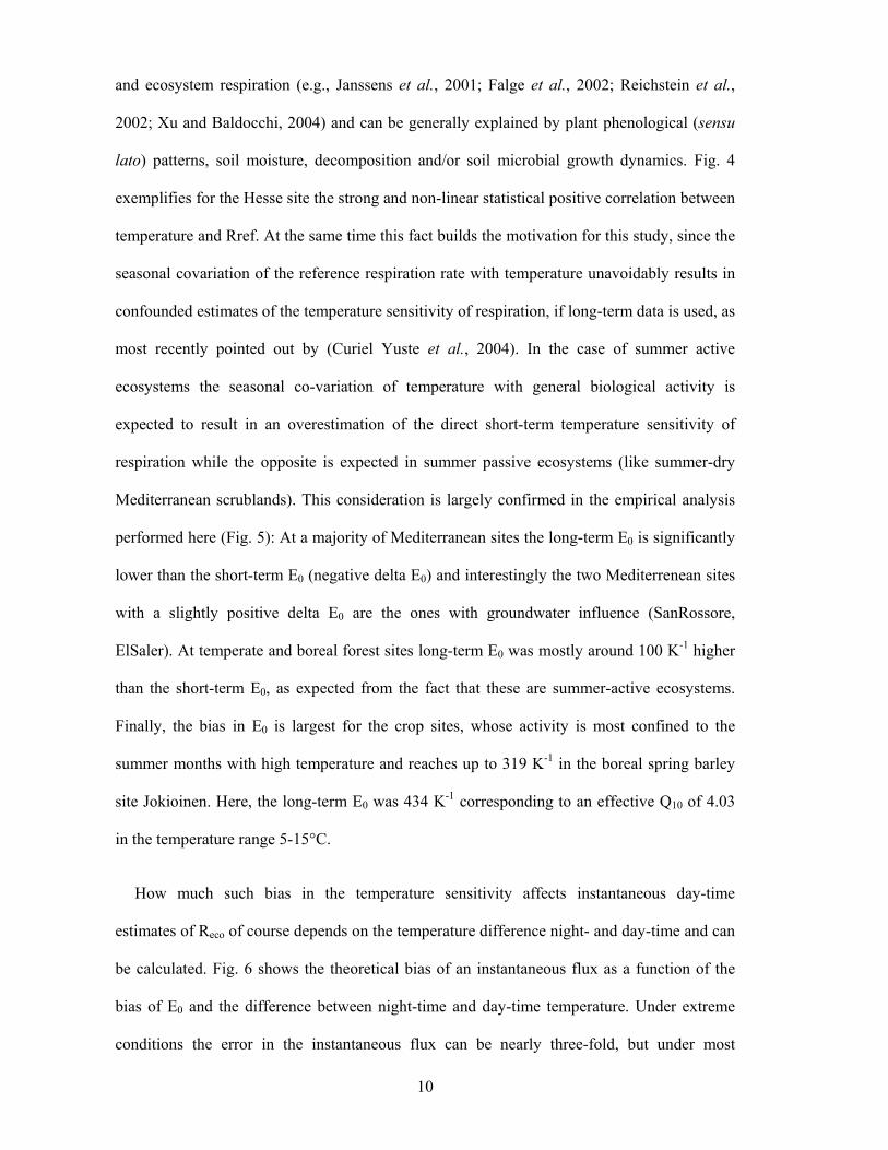
and ecosystem respiration (e.g., Janssens et al., 2001; Falge et al., 2002; Reichstein et al.,

2002; Xu and Baldocchi, 2004) and can be generally explained by plant phenological (sensu

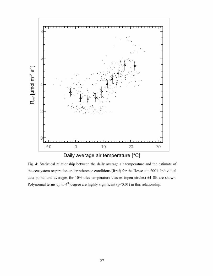
lato) patterns, soil moisture, decomposition and/or soil microbial growth dynamics. Fig. 4

exemplifies for the Hesse site the strong and non-linear statistical positive correlation between

temperature and Rref. At the same time this fact builds the motivation for this study, since the

seasonal covariation of the reference respiration rate with temperature unavoidably results in

confounded estimates of the temperature sensitivity of respiration, if long-term data is used, as

most recently pointed out by (Curiel Yuste et al., 2004). In the case of summer active

ecosystems the seasonal co-variation of temperature with general biological activity is

expected to result in an overestimation of the direct short-term temperature sensitivity of

respiration while the opposite is expected in summer passive ecosystems (like summer-dry

Mediterranean scrublands). This consideration is largely confirmed in the empirical analysis

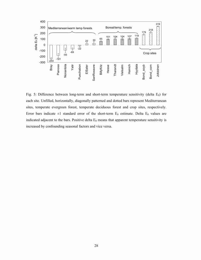
performed here (Fig. 5): At a majority of Mediterranean sites the long-term E0 is significantly

lower than the short-term E0 (negative delta E0) and interestingly the two Mediterrenean sites

with a slightly positive delta E0 are the ones with groundwater influence (SanRossore,

ElSaler). At temperate and boreal forest sites long-term E0 was mostly around 100 K-1 higher

than the short-term E0, as expected from the fact that these are summer-active ecosystems.

Finally, the bias in E0 is largest for the crop sites, whose activity is most confined to the

summer months with high temperature and reaches up to 319 K-1 in the boreal spring barley

site Jokioinen. Here, the long-term E0 was 434 K-1 corresponding to an effective Q10 of 4.03

in the temperature range 5-15°C.

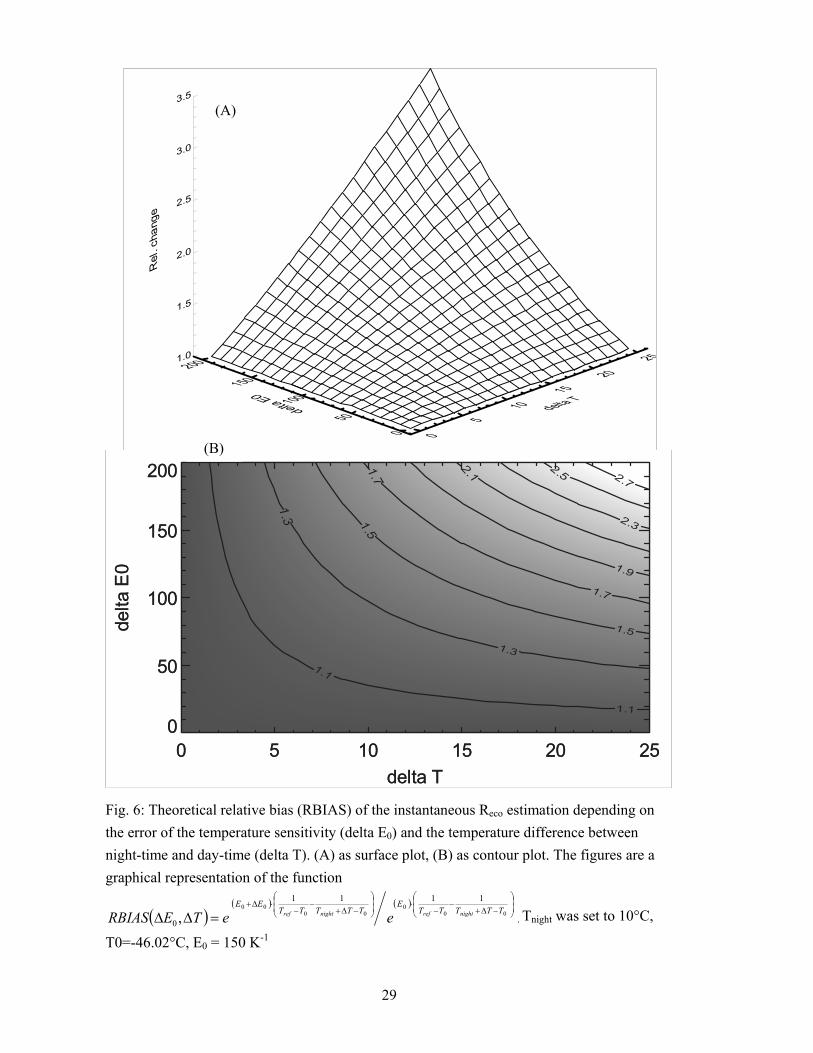
How much such bias in the temperature sensitivity affects instantaneous day-time

estimates of Reco of course depends on the temperature difference night- and day-time and can

be calculated. Fig. 6 shows the theoretical bias of an instantaneous flux as a function of the

bias of E0 and the difference between night-time and day-time temperature. Under extreme

conditions the error in the instantaneous flux can be nearly three-fold, but under most

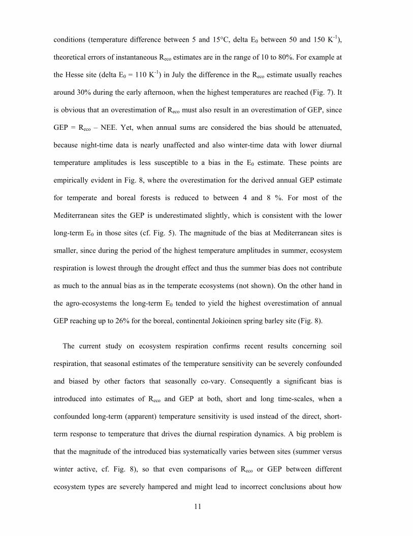
11

conditions (temperature difference between 5 and 15°C, delta E0 between 50 and 150 K-1),

theoretical errors of instantaneous Reco estimates are in the range of 10 to 80%. For example at

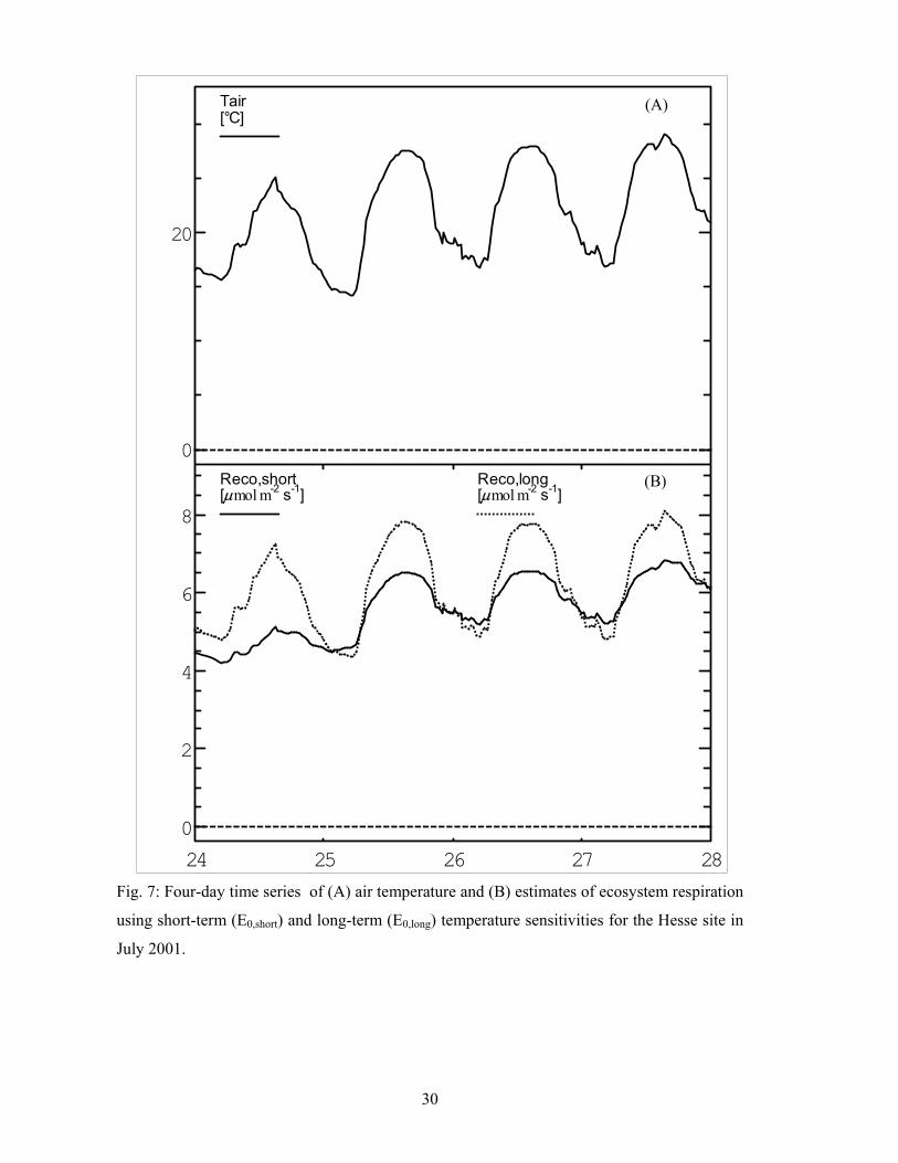
the Hesse site (delta E0 = 110 K-1) in July the difference in the Reco estimate usually reaches

around 30% during the early afternoon, when the highest temperatures are reached (Fig. 7). It

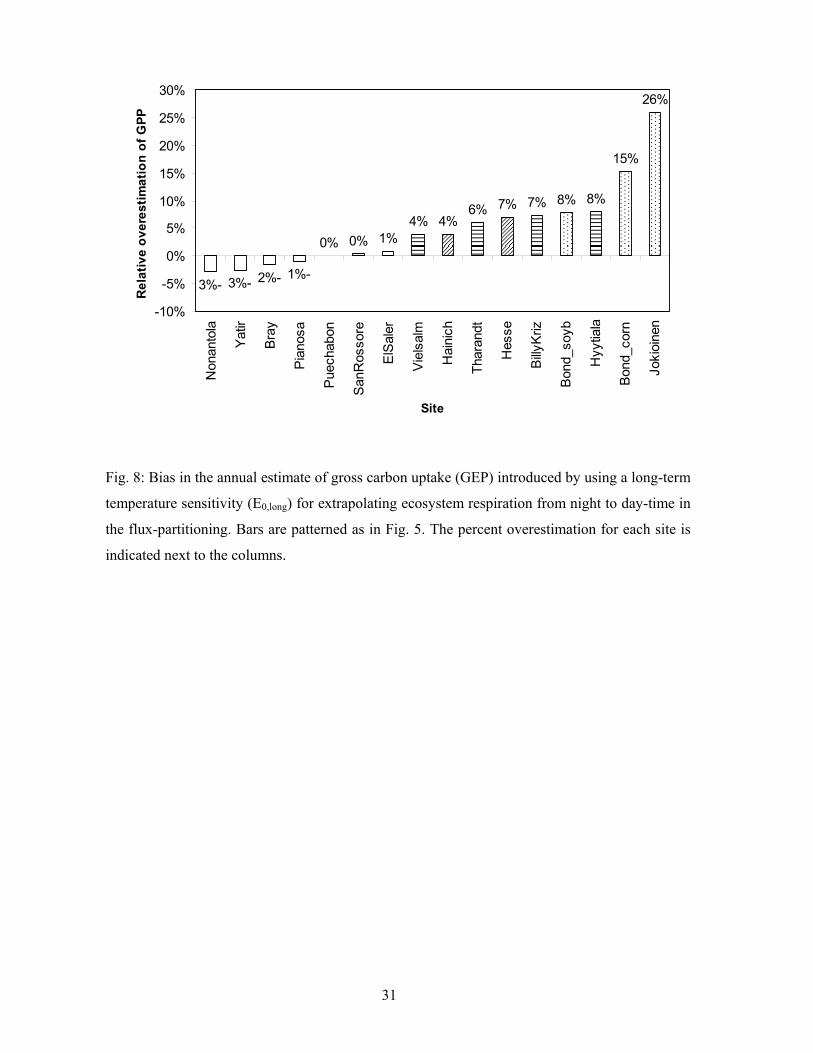
is obvious that an overestimation of Reco must also result in an overestimation of GEP, since

GEP = Reco – NEE. Yet, when annual sums are considered the bias should be attenuated,

because night-time data is nearly unaffected and also winter-time data with lower diurnal

temperature amplitudes is less susceptible to a bias in the E0 estimate. These points are

empirically evident in Fig. 8, where the overestimation for the derived annual GEP estimate

for temperate and boreal forests is reduced to between 4 and 8 %. For most of the

Mediterranean sites the GEP is underestimated slightly, which is consistent with the lower

long-term E0 in those sites (cf. Fig. 5). The magnitude of the bias at Mediterranean sites is

smaller, since during the period of the highest temperature amplitudes in summer, ecosystem

respiration is lowest through the drought effect and thus the summer bias does not contribute

as much to the annual bias as in the temperate ecosystems (not shown). On the other hand in

the agro-ecosystems the long-term E0 tended to yield the highest overestimation of annual

GEP reaching up to 26% for the boreal, continental Jokioinen spring barley site (Fig. 8).

The current study on ecosystem respiration confirms recent results concerning soil

respiration, that seasonal estimates of the temperature sensitivity can be severely confounded

and biased by other factors that seasonally co-vary. Consequently a significant bias is

introduced into estimates of Reco and GEP at both, short and long time-scales, when a

confounded long-term (apparent) temperature sensitivity is used instead of the direct, short-

term response to temperature that drives the diurnal respiration dynamics. A big problem is

that the magnitude of the introduced bias systematically varies between sites (summer versus

winter active, cf. Fig. 8), so that even comparisons of Reco or GEP between different

ecosystem types are severely hampered and might lead to incorrect conclusions about how

12

continental and environmental gradients affect Reco and GEP. Moreover, since the bias is

dependent on the diurnal temperature amplitude (cf. Fig. 6) – the higher the temperature

amplitude the larger the bias – it also changes seasonally and affects conclusions about

seasonality of Reco and GEP. This seasonal bias is also critical for model evaluations that are

often performed at the seasonal time-scale.

The algorithm introduced here was able to find a short-term temperature response of Reco at

all studied sites and is a significant step forward towards less biased estimates of Reco and

GEP. But it is not guaranteed to work at all sites since whether one can find a reliable short-

term relationship between Reco and temperature depends on the noisiness of the eddy data and

the range of temperatures encompassed during the short period. At sites with very stable

temperatures and noisy eddy covariance data, it might be possible that within a year no short

period can be found where a temperature-Reco relationship can be established. And finally,

seasonal changes in the temperature sensitivity that have been hypothesized are hard to detect

from eddy covariance data, since in many cases not enough short-term periods with a good

relationship between temperature and Reco were found to make up a seasonality. Moreover, it

cannot be excluded that even with the method presented here still other factors are

confounding the relationship between T and Reco. In particular, if leaf dark respiration is light-

inhibited during the day (Kok, 1948), day-time ecosystem respiration would be overestimated

when extrapolating from night-time data. However, recent findings using stable-isotope

methodology show that under most conditions the light-inhibition of leaf dark respiration is

only apparent and a result of CO2 re-fixation in the leaf (Loreto et al., 2001; Pinelli and

Loreto, 2003). In this situation there is no diurnal bias introduced into the day-time Reco and

GPP estimate. Nevertheless, we recommend that the flux-partitioning would be helped a lot

with independent estimates of the short-term sensitivity of respiration to temperature of the

main respiring component with chamber methods.

13

Conclusion

For understanding the effect of spatial and environmental gradients on ecosystem net

ecosystem exchange (NEE) from eddy covariance data it is essential to acquire estimates of

its main components, ecosystem respiration (Reco) and gross primary production (GEP),

through a so-called flux-partitioning algorithm. A number of methods are available for this

task but with all methods biased estimates of GEP and Reco are likely through the effect of

confounding factors. Here we show that using a temperature-Reco relationship from seasonal

data (that is confounded, e.g. by growth dynamics, and soil drought effects), can introduce a

significant bias into Reco and GEP estimates from hourly to annual time-scales. Thus we

introduce and recommend using an algorithm that defines a short-term temperature sensitivity

of ecosystem respiration and thus largely avoids the bias introduced by confounding factors in

seasonal data. Particularly in cases, where no reliable short-term relationship between

temperature (or another more relevant diurnally varying factor) and Reco can be found from

eddy covariance data such a relationship should be established via observing the main

respiring components with chamber methods.

Acknowledgements

Data collection was funded by the CARBOEUROFLUX and AMERIFLUX projects, that

are organized in the FLUXNET network. The analysis was supported by a European Marie-

Curie fellowship to MR (MEIF-CT-2003-500696).

References

Aubinet M, Chermanne B, Vandenhaute M, et al. (2001) Long term carbon dioxide exchange above a mixed forest in the Belgian Ardennes. Agricultural and Forest Meteorology, 108.

Aubinet M, Grelle A, Ibrom A, et al. (2000) Estimates of the annual net carbon and water exchange of forests: the euroflux methodology. Advances in Ecological Research, 30, 113-175.

Baldocchi D, Falge E, Gu LH, et al. (2001) FLUXNET: A new tool to study the temporal and spatial variability of ecosystem-scale carbon dioxide, water vapor, and energy flux densities. Bulletin of the American Meteorological Society, 82, 2415-2434.

14

Baldocchi DD (1997) Measuring and modelling carbon dioxide and water vapour exchange over a temperate broad-leaved forest during the 1995 summer drought. Plant, Cell and Environment, 20, 1108-1122.

Baldocchi DD, Meyers T (1998) On using-ecophysiological, micrometeorological and biogeochemical theory to evaluate carbon dioxide, water vapor and trace gas fluxes over vegetation: a perspective. Agricultural and Forest Meteorology, 90, 1-25.

Berbigier P, Bonnefond JM, Mellmann P (2001) CO2 and water vapour fluxes for 2 years above Euroflux forest site. Agricultural and Forest Meteorology, 108, 183-197.

Bernhofer C, Aubinet M, Clement R, et al. (2003) Spruce Forests (Norway and Sitka Spruce, Including Douglas Fir): Carbon and Water Fluxes, Balances, Ecological and Ecophysiological Determinants. In: Fluxes of Carbon, Water and Energy of European Forests. Ecological Studies 163. (ed. R. Valentini), p. 99-122. Springer, Heidelberg.

Curiel Yuste J, Janssens IA, Carrara A, Ceulemanns R (2004) Annual Q10 of soil respiration reflects plant phenological patterns as well as temperature sensitivity. Global Change Biology, 10, 161-169.

Davidson EA, Belk E, Boone RD (1998) Soil water content and temperature as independent or confounded factors controlling soil respiration in temperate mixed hardwood forest. Global Change Biology, 4, 217-227.

Falge E, Baldocchi D, Olson R, et al. (2001) Gap filling strategies for long term energy flux data sets. Agricultural and Forest Meteorology, 107, 71-77.

Falge E, Baldocchi D, Olson R, et al. (2001) Gap filling strategies for defensible annual sums of net ecosystem exchange. Agricultural and Forest Meteorology, 107, 43-69.

Falge E, Baldocchi D, Tenhunen J, et al. (2002) Seasonality of ecosystem respiration and gross primary production as derived from FLUXNET measurements. Agricultural and Forest Meteorology, 113, 53-74.

Falge E, Tenhunen J, Baldocchi D, et al. (2002) Phase and amplitude of ecosystem carbon release and uptake potentials as derived from FLUXNET measurements. Agricultural and Forest Meteorology, 113, 75-95.

Foken T, Wichura B (1996) Tools for quality assessment of surface-based flux measurements. Agricultural and Forest Meteorology, 78, 83-105.

Georgiadis T, Magliulo E, Miglietta F, et al. (2002) A contribution to Pianosa-LAB from Agenzia. An advanced ground based network for the study of gas exchanges between terrestrial vegetation and the atmosphere. In: Proceedings of the First Italian IGBP Conference, p. 41-42, Paestum.

Gilmanov TG, Verma SB, Sims PL, et al. (2003) Gross primary production and light response parameters of four Southern Plains ecosystems estimated using long-term CO2-flux tower measurements. Global Biogeochemical Cycles, 17, 1071, doi: 1010.1029/2002GB002023.

Granier A, Ceschia E, Damesin C, et al. (2000) The carbon balance of a young beech forest. Functional Ecology, 14, 312-325.

Grünzweig JM, Lin T, Rotenberg E, et al. (2003) Carbon sequestration in arid-land forest. Global Change Biology, 9, 791-799.

Hanan NP, Burba G, Verma S, et al. (2002) Inversion of net ecosystem CO2 flux measurements for estimation of canopy PAR absorption. Global Change Biology, 8, 563-574.

Hollinger D, Kelliher F, Byers J, et al. (1994) Carbon dioxide exchange between an undisturbed old-growth temperate forest and the atmosphere. Ecology, 75, 134-150.

Hollinger DY, Kelliher FM, Schulze ED, et al. (1998) Forest-atmosphere carbon dioxide exchange in eastern siberia. Agricultural and Forest Meteorology, 90, 291-306.

Hui D, Wan S, Su B, et al. (2003) Gap-filling missing data in eddy covariance measurements by multiple imputation (MI) for annual estimations. Agricultural and Forest Meteorology, 121.

15

Janssens IA, Lankreijer H, Matteucci G, et al. (2001) Productivity overshadows temperature in determining soil and ecosystem respiration across European forests. Global Change Biology, 7, 269-278.

Knohl A, Schulze E-D, Kolle O, Buchmann N (2003) Large carbon uptake by an unmanaged 250-year-old deciduous forest in Central Germany. Agricultural and Forest Meteorology, 118, 151-167.

Kok B (1948) A critical consideration of the quantum yield of Chlorella-photosynthesis. Enzymologia, 13, 1-56.

Law BE, Baldocchi DD, Anthoni PM (1999) Below-canopy and soil CO2 fluxes in a ponderosa pine forest. Agricultural and Forest Meteorology, 94, 171-188.

Law BE, Falge E, Baldocchi DD, et al. (2002) Environmental controls over carbon dioxide and water vapor exchange of terrestrial vegetation. Agricultural and Forest Meteorology, 113, 97-120.

Law BE, Kelliher FM, Baldocchi DD, et al. (2001) Spatial and temporal variation in respiration in a young ponderosa pine forest during a summer drought. Agricultural and Forest Meteorology, 110, 27-43.

Law BE, Thornton P, Irvine J, et al. (2001) Carbon storage and fluxes in ponderosa pine forests at different developmental stages. Global Change Biology, 7, 755-777.

Lloyd J, Taylor JA (1994) On the temperature dependence of soil respiration. Functional Ecology, 8, 315-323.

Lohila A, Aurela M, Tuovinen J-P, Laurila T (in press) Annual CO2 exchange of a peat field growing spring barley or perennial forage grass. Journal of Geophysical Research, 0000, 0000-0000.

Loreto F, Velikova V, Di Marco G (2001) Respiation in the light measured by 12CO2 emission in 13CO2 atmosphere in maize leaves. Australian Journal of Plant Physiology, 28, 1103-1108.

Nardino M, Miglietta F, Georgiadis T, et al. (2002) CO2, water and heat fluxes in a Kyoto-reforestation. In: Proceeding of the First Italian IGBP Conference, p. 37-39, Paestum.

Papale D, Valentini R (2002) A new assessment of European forests carbon exhcanges by eddy fluxes and artificial neural network spatialization. Global Change Biology, 9, 525-535.

Pinelli P, Loreto F (2003) 12CO2 emission from different metabolic pathways measured in illuminated and darkened C3 and C4 leaves at low, atmospheric and elevated CO2 concentration. Journal of Experimental Botany, 54, 1761-1769.

Rambal S, Ourcival J-M, Joffre R, et al. (2003) Drought controls over conductance and assimilation of a Mediterranean evergreen ecosystem: scaling from leaf to canopy. Global Change Biology, 9, 1813-1824; doi: 1810.1046/j.1529-8817.2003.00687.x.

Rannik Ü, Altimir N, Raittila J, et al. (2002) Fluxes of carbon dioxide and water vapour over Scots pine forest and clearing. Agricultural and Forest Meteorology, 111, 187-202.

Reichstein M, Dinh N, Running S, et al. (2003) Towards improved European carbon balance estimates through assimilation of MODIS remote sensing data and CARBOEUROPE eddy covariance observations into an advanced ecosystem and statistical modeling system. In: Proceedings of the International Geoscience and Remote Sensing Symposium (IGARSS'03), Toulouse, France, 21-25 July 2003.

Reichstein M, Tenhunen J, Ourcival J-M, et al. (2003) Inverse modelling of easonal drought effects on canopy CO2/H2O exchange in three Mediterranean Ecosystems. Journal of Geophysical Research, 108, D23, 4726, 4716/4721-4716/4716, doi:4710.1029/2003JD003430,.

Reichstein M, Tenhunen JD, Ourcival JM, et al. (2002) Ecosystem respiration in two mediterranean evergreen holm oak forests: drought effects and decomposition dynamics. Functional Ecology, 16, 27-39.

16

Reichstein M, Tenhunen JD, Ourcival J-M, et al. (2002) Severe drought effects on ecosystem CO2 and H2O fluxes at three mediterranean sites: revision of current hypothesis? Global Change Biology, 8, 999-1017.

Sanz MJ, Carrara A, Gimeno C, et al. (2004) Effects of a dry and warm summer conditions on CO2 and Energy fluxes from three Mediterranean ecosystems. Geophysical Research Abstracts, 6, 03239-03239.

Subke J-A, Reichstein M, Tenhunen M (2003) Explaining temporal variation in soil CO2 efflux in a mature spruce forest in Southern Germany. Soil Biology & Biochemistry, 35, 1467-1483.

Valentini R, Matteucci G, Dolman AJ, et al. (2000) Respiration as the main determinant of carbon balance in European forests. Nature, 404, 861-865.

Xu L, Baldocchi DD (2004) Seasonal variation in carbon dioxide exchange over a Mediterranean annual grassland in California. Agricultural and Forest Meteorology, 123, 79-96.

Xu M, Qi Y (2001) soil-surface CO2 efflux and its spatial and temporal variations in a young ponderosa pine plantation in northern california. Global Change Biology, 7, 667-677.

17

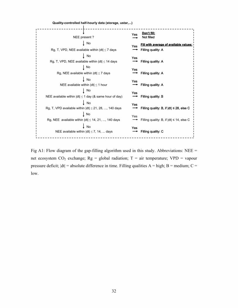
Appendix – Gap-filling methodology

The gap-filling of the eddy covariance and meteorological data will be performed through

methods that are similar to Falge et al. (2001), but that consider both the co-variation of

fluxes with meteorological variables and the temporal auto-correlation of the fluxes: In this

algorithm, three different conditions are identified: 1) Only the data of direct interest are

missing, but all meteorological data are available, 2) Also air temperature or VPD is missing,

but radiation is available, 3) Also radiation data is missing. In case 1), the missing value is

replaced by the average value under similar meteorological conditions within a time-window

of ±7 days. Similar meteorological conditions are present when Rg, Tair and VPD do not

deviate by more than 50 W m-2, 2.5 °C, and 5.0 hPa respectively. If no similar meteorological

conditions are present within the time window, the averaging window is increased to ±14

days. In case 2) the same approach is taken, but similar meteorological conditions can only be

defined via Rg deviation less than 50 W m-2 and the window size is first not further increased.

In case 3) the missing value is replaced by the average value at the same time of the day (± 1

hour), i.e. by the mean diurnal course. In this case the window size starts with ± 0.5 days (i.e.

similar to a linear interpolation from available data at adjacent hours). If after these steps the

values could not be filled, the procedure is repeated with increased window sizes until the

value can be filled. Fig. A1 summarizes the algorithm. Both, the method, the window size,

and the number and the standard deviation of values averaged is recorded then, so that for

individual purposes appropriate data can be selected and e.g. uncertainties can be estimated.

For convenience, the filled data is further classified into three tentative categories (A, B, C)

based on the method (1, 2, or 3) and the window size used (Fig. A1). The classification is

based on the notion, that the estimation of the missing data improves with the knowledge on

meteorological conditions and with the use of the temporal auto-correlation of the variable

that favours smaller time-windows.

18

Tables

Table 1 : Classification of currently available statistical flux-partitioning algorithms of eddy covariance net CO2 flux data

Algorithm Advantages Disadvantages

A: Using only night-time data Flux data is directly used, i.e. direct estimation of Reco

Filtering of bad night-time data necessary, extrapolation to day-time necessary

1. Representation of Reco by one single function of temperature (Hollinger et al., 1994)

Simplicity Only applicable where no other factors than temperature influence Reco significantly, not generic

2. Representation of Reco by one single function of temperature and other factors (Reichstein et al., 2002; Rambal et al., 2003)

Simplicity, not only temperature as factor considered; allows for seasonally varying temperature sensitivity

Results in selection of site specific factors that determine Reco, not generic

3. Representation of Reco by temporally varying functions of temperature (Rref varying, one single temperature sensitivity derived from annual data set (Falge et al., 2002; Law et al., 2002)

Accounts for temporally varying respiration rates at reference temperature, caused by any factor

Long-term temperature sensitivity from annual data set may not reflect short-term response, introduction of systematic error when extrapolating to day-time

4. Representation of Reco by temporally varying functions of temperature (Rref varying, one single temperature sensitivity derived from short-term data set (this study)

Accounts for temporally varying respiration rates at reference temperature, caused by any factor, ‘correct’ temperature response avoids introduction of systematic error when extrapolating to day-time

Seasonally varying temperature sensitivity not accounted for

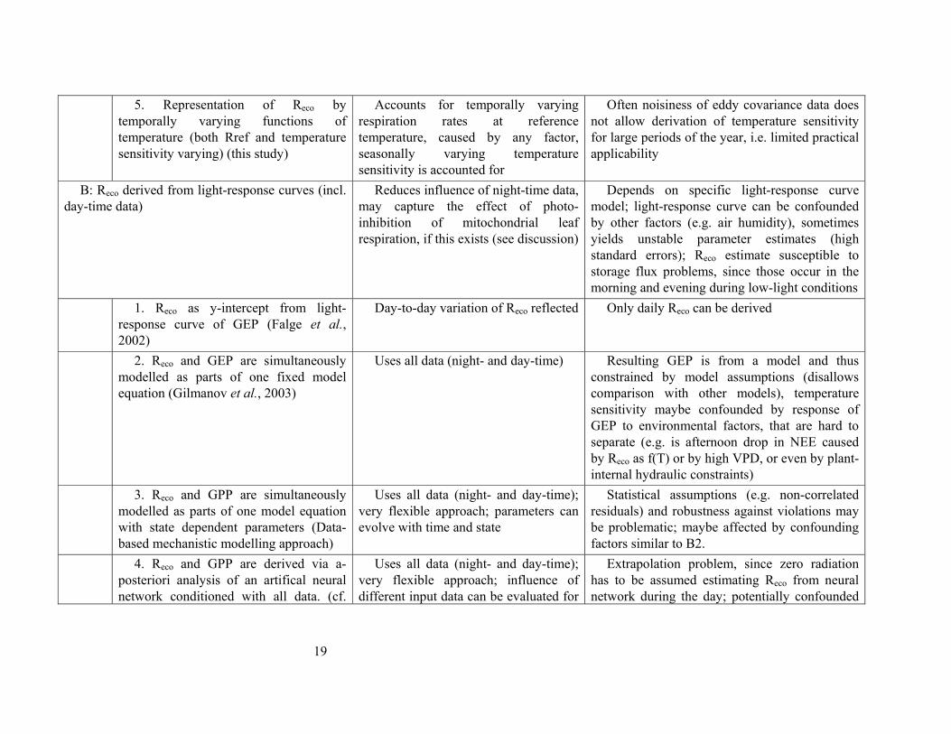
19

5. Representation of Reco by temporally varying functions of temperature (both Rref and temperature sensitivity varying) (this study)

Accounts for temporally varying respiration rates at reference temperature, caused by any factor, seasonally varying temperature sensitivity is accounted for

Often noisiness of eddy covariance data does not allow derivation of temperature sensitivity for large periods of the year, i.e. limited practical applicability

B: Reco derived from light-response curves (incl. day-time data)

Reduces influence of night-time data, may capture the effect of photo-inhibition of mitochondrial leaf respiration, if this exists (see discussion)

Depends on specific light-response curve model; light-response curve can be confounded by other factors (e.g. air humidity), sometimes yields unstable parameter estimates (high standard errors); Reco estimate susceptible to storage flux problems, since those occur in the morning and evening during low-light conditions

1. Reco as y-intercept from light-response curve of GEP (Falge et al., 2002)

Day-to-day variation of Reco reflected Only daily Reco can be derived

2. Reco and GEP are simultaneously modelled as parts of one fixed model equation (Gilmanov et al., 2003)

Uses all data (night- and day-time) Resulting GEP is from a model and thus constrained by model assumptions (disallows comparison with other models), temperature sensitivity maybe confounded by response of GEP to environmental factors, that are hard to separate (e.g. is afternoon drop in NEE caused by Reco as f(T) or by high VPD, or even by plant-internal hydraulic constraints)

3. Reco and GPP are simultaneously modelled as parts of one model equation with state dependent parameters (Data-based mechanistic modelling approach)

Uses all data (night- and day-time); very flexible approach; parameters can evolve with time and state

Statistical assumptions (e.g. non-correlated residuals) and robustness against violations may be problematic; maybe affected by confounding factors similar to B2.

4. Reco and GPP are derived via a-posteriori analysis of an artifical neural network conditioned with all data. (cf.

Uses all data (night- and day-time); very flexible approach; influence of different input data can be evaluated for

Extrapolation problem, since zero radiation has to be assumed estimating Reco from neural network during the day; potentially confounded

20

(Papale and Valentini, 2002) for gap-filling; flux-partitioning not explored)

best description of the data set by other factors similar to B2.

21

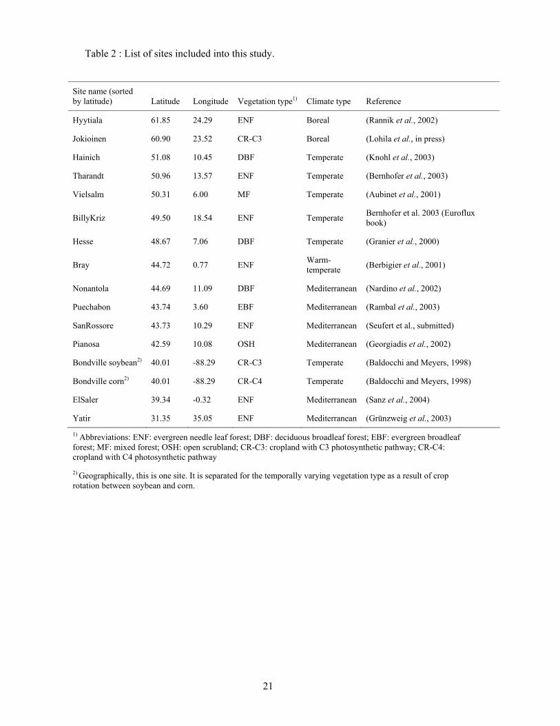
Table 2 : List of sites included into this study.

Site name (sorted by latitude) Latitude Longitude Vegetation type1) Climate type Reference

Hyytiala 61.85 24.29 ENF Boreal (Rannik et al., 2002)

Jokioinen 60.90 23.52 CR-C3 Boreal (Lohila et al., in press)

Hainich 51.08 10.45 DBF Temperate (Knohl et al., 2003)

Tharandt 50.96 13.57 ENF Temperate (Bernhofer et al., 2003)

Vielsalm 50.31 6.00 MF Temperate (Aubinet et al., 2001)

BillyKriz 49.50 18.54 ENF Temperate Bernhofer et al. 2003 (Euroflux book)

Hesse 48.67 7.06 DBF Temperate (Granier et al., 2000)

Bray 44.72 0.77 ENF Warm-temperate (Berbigier et al., 2001)

Nonantola 44.69 11.09 DBF Mediterranean (Nardino et al., 2002)

Puechabon 43.74 3.60 EBF Mediterranean (Rambal et al., 2003)

SanRossore 43.73 10.29 ENF Mediterranean (Seufert et al., submitted)

Pianosa 42.59 10.08 OSH Mediterranean (Georgiadis et al., 2002)

Bondville soybean2) 40.01 -88.29 CR-C3 Temperate (Baldocchi and Meyers, 1998)

Bondville corn2) 40.01 -88.29 CR-C4 Temperate (Baldocchi and Meyers, 1998)

ElSaler 39.34 -0.32 ENF Mediterranean (Sanz et al., 2004)

Yatir 31.35 35.05 ENF Mediterranean (Grünzweig et al., 2003)

1) Abbreviations: ENF: evergreen needle leaf forest; DBF: deciduous broadleaf forest; EBF: evergreen broadleaf forest; MF: mixed forest; OSH: open scrubland; CR-C3: cropland with C3 photosynthetic pathway; CR-C4: cropland with C4 photosynthetic pathway

2) Geographically, this is one site. It is separated for the temporally varying vegetation type as a result of crop rotation between soybean and corn.

22

Figure legends

Fig. 1: Schematic representation of the confounding effects introduced into a temperature

dependence of ecosystem respiration derived from annual data. Triangles and squares are

hypothetical data for summer active and summer passive ecosystems, respectively.

Fig. 2: Schematic representation of the parameter estimation for calculating ecosystem

respiration. (A) The half-hourly night-time CO2 net ecosystem exchange; (B) the half-hourly

night-time air temperature, (C) the derived Lloyd-and-Taylor model parameters. E0 is

estimated from the best regression of the total data set, while Rref is estimated locally for the

periods indicated by the bars in (A) and subsequently interpolated. See text for details.

Fig. 3: Time series (A,B) of derived Lloyd-and-Taylor (1994) parameters (cf. Eq. 2), (C) air

temperature, and (D) derived ecosystem respiration for the Hesse site

Fig. 4: Statistical relationship between the daily average air temperature and the estimate of

the ecosystem respiration under reference conditions (Rref) for the Hesse site 2001. Individual

data points and averages for 10%-tiles temperature classes (open circles) ±1 SE are shown.

Polynomial terms up to 4th degree are highly significant (p<0.01) in this relationship.

Fig. 5: Difference between long-term and short-term temperature sensitivity (delta E0) for

each site. Unfilled, horizontally, diagonally patterned and dotted bars represent Mediterranean

sites, temperate evergreen forest, temperate deciduous forest and crop sites, respectively.

Error bars indicate ±1 standard error of the short-term E0 estimate. Delta E0 values are

indicated adjacent to the bars. Positive delta E0 means that apparent temperature sensitivity is

increased by confounding seasonal factors and vice versa.

Fig. 6: Theoretical relative bias (RBIAS) of the instantaneous Reco estimation depending on the error of the temperature sensitivity (delta E0) and the temperature difference between night-time and day-time (delta T). (A) as surface plot, (B) as contour plot. The figures are a graphical representation of the function

( )( ) ( )

−∆+−

−⋅

−∆+−

−⋅∆+

=∆∆ 000

0000

1111

0 , TTTTTE

TTTTTEE

nightrefnightref eeTERBIAS . Tnight was set to 10°C,

T0=-46.02°C, E0 = 150 K-1

Fig. 7: Four-day time series of (A) air temperature and (B) estimates of ecosystem respiration

using short-term (E0,short) and long-term (E0,long) temperature sensitivities for the Hesse site in

July 2001.

23

Fig. 8: Bias in the annual estimate of gross carbon uptake (GEP) introduced by using a long-

term temperature sensitivity (E0,long) for extrapolating ecosystem respiration from night to

day-time in the flux-partitioning. Bars are patterned as in Fig. 5. The percent overestimation

for each site is indicated next to the columns.

Fig A1: Flow diagram of the gap-filling algorithm used in this study. Abbreviations: NEE =

net ecosystem CO2 exchange; Rg = global radiation; T = air temperature; VPD = vapour

pressure deficit; |dt| = absolute difference in time. Filling qualities A = high; B = medium; C =

low.

24

Figures

Temperature

Res

pira

tion

Confounded responsesummer active

Confounded responsesummer passive

Direct ‚true‘ response to temperature

Temperature

Res

pira

tion

Confounded responsesummer active

Confounded responsesummer passive

Direct ‚true‘ response to temperature

Temperature

Res

pira

tion

Confounded responsesummer active

Confounded responsesummer passive

Direct ‚true‘ response to temperature

Fig. 1: Schematic representation of the confounding effects introduced into a temperature

dependence of ecosystem respiration derived from annual data. Triangles and squares are

hypothetical data for summer active and summer passive ecosystems, respectively.

25

Fig. 2: Schematic representation of the parameter estimation for calculating ecosystem

respiration. (A) The half-hourly night-time CO2 net ecosystem exchange; (B) the half-hourly

night-time air temperature, (C) the derived Lloyd-and-Taylor model parameters. E0 is estimated

from the best regression of the total data set, while Rref is estimated locally for the periods

indicated by the bars in (A) and subsequently interpolated. See text for details.

0

2

4

6

8

10

120 121 122 123 124 125 126 127 128 129 130 131 132 133 134 135 136

0

5

10

15

20

25

120 121 122 123 124 125 126 127 128 129 130 131 132 133 134 135 136

0

1

2

3

4

5

120 121 122 123 124 125 126 127 128 129 130 131 132 133 134 135 1360

50

100

150

200

250

300

0

2

4

6

8

10

120 121 122 123 124 125 126 127 128 129 130 131 132 133 134 135 136

0

5

10

15

20

25

120 121 122 123 124 125 126 127 128 129 130 131 132 133 134 135 136

0

1

2

3

4

5

120 121 122 123 124 125 126 127 128 129 130 131 132 133 134 135 1360

50

100

150

200

250

300E0E0

Rref

NEE

(nig

ht)

[µm

ol m

-2s-

1 ]Ta

ir (n

ight

)[°

C]

Rre

f[µ

mol

m-2

s-1 ]

E 0[K

-1]

(A)

(B)

(C)

26

0

200

E0short[K-1]

E0long[K-1]

0

2

4

6

8

10 Rref[µmol m-2 s-1]

-10

0

10

20

30Tair[°C]

Jan Feb M ar Apr M ay Jun Jul Aug Sep Oct Nov Dec2001 2002

0

2

4

6

8

10

12 Reco[µmol m-2 s-1]

Fig. 3: Time series (A,B) of derived Lloyd-and-Taylor (1994) parameters (cf. Eq. 2), (C) air

temperature, and (D) derived ecosystem respiration for the Hesse site

(A)

(B)

(C)

(D)

27

-10 0 10 20 30

0

2

4

6

8

Daily average air temperature [°C]

Rre

f[µ

mol

m-2

s-1]

Fig. 4: Statistical relationship between the daily average air temperature and the estimate of

the ecosystem respiration under reference conditions (Rref) for the Hesse site 2001. Individual

data points and averages for 10%-tiles temperature classes (open circles) ±1 SE are shown.

Polynomial terms up to 4th degree are highly significant (p<0.01) in this relationship.

28

-233

65101 104 104 107 119

179218

319

3022

-22-69

-93

-181-300

-200

-100

0

100

200

300

400

Bra

y

Pia

nosa

Non

anto

la

Yat

ir

Pue

chab

on

ElS

aler

San

Ros

sore

Billy

Kriz

Hes

se

Thar

andt

Vie

lsal

m

Hai

nich

Hyy

tiala

Bon

d_so

yb

Bon

d_co

rn

Joki

oine

n

delta

E0 [

K-1

]

Mediterranean/warm temp forests Boreal/temp. forests

Crop sites

-233

65101 104 104 107 119

179218

319

3022

-22-69

-93

-181-300

-200

-100

0

100

200

300

400

Bra

y

Pia

nosa

Non

anto

la

Yat

ir

Pue

chab

on

ElS

aler

San

Ros

sore

Billy

Kriz

Hes

se

Thar

andt

Vie

lsal

m

Hai

nich

Hyy

tiala

Bon

d_so

yb

Bon

d_co

rn

Joki

oine

n

delta

E0 [

K-1

]

Mediterranean/warm temp forests Boreal/temp. forests

Crop sites

Fig. 5: Difference between long-term and short-term temperature sensitivity (delta E0) for

each site. Unfilled, horizontally, diagonally patterned and dotted bars represent Mediterranean

sites, temperate evergreen forest, temperate deciduous forest and crop sites, respectively.

Error bars indicate ±1 standard error of the short-term E0 estimate. Delta E0 values are

indicated adjacent to the bars. Positive delta E0 means that apparent temperature sensitivity is

increased by confounding seasonal factors and vice versa.

29

0 5 10 15 20 25delta T

0

50

100

150

200

delta

E0

1.1

1.1

1.3

1.3

1.5

1.51.7

1.7

1.9

2.1

2.3

2.5 2.7

0 5 10 15 20 25delta T

0

50

100

150

200

delta

E0

1.1

1.1

1.3

1.3

1.5

1.51.7

1.7

1.9

2.1

2.3

2.5 2.7

Fig. 6: Theoretical relative bias (RBIAS) of the instantaneous Reco estimation depending on the error of the temperature sensitivity (delta E0) and the temperature difference between night-time and day-time (delta T). (A) as surface plot, (B) as contour plot. The figures are a graphical representation of the function

( )( ) ( )

−∆+−

−⋅

−∆+−

−⋅∆+

=∆∆ 000

0000

1111

0 , TTTTTE

TTTTTEE

nightrefnightref eeTERBIAS . Tnight was set to 10°C,

T0=-46.02°C, E0 = 150 K-1

05

1015

2025

delta T

050

100150

200

delta E0

1.0

1.5

2.0

2.5

3.0

3.5

Rel

. cha

nge

(A)

(B)

30

0

20

Tair[°C]

24 25 26 27 28

0

2

4

6

8

Reco,short[µmol m-2 s-1]

Reco,long[µmol m-2 s-1]

Fig. 7: Four-day time series of (A) air temperature and (B) estimates of ecosystem respiration

using short-term (E0,short) and long-term (E0,long) temperature sensitivities for the Hesse site in

July 2001.

(A)

(B)

31

3%- 3%- 2%- 1%-

0% 0% 1%4% 4%

6% 7% 7% 8% 8%

15%

26%

-10%

-5%

0%

5%

10%

15%

20%

25%

30%

Non

anto

la

Yatir

Bra

y

Pian

osa

Puec

habo

n

SanR

osso

re

ElSa

ler

Viel

salm

Hai

nich

Thar

andt

Hes

se

Billy

Kriz

Bond

_soy

b

Hyy

tiala

Bond

_cor

n

Joki

oine

n

Site

Rel

ativ

e ov

eres

timat

ion

of G

PP

Fig. 8: Bias in the annual estimate of gross carbon uptake (GEP) introduced by using a long-term

temperature sensitivity (E0,long) for extrapolating ecosystem respiration from night to day-time in

the flux-partitioning. Bars are patterned as in Fig. 5. The percent overestimation for each site is

indicated next to the columns.

32

Rg, NEE available within |dt| ≤ 7 days

NEE available within |dt| ≤ 1 hour

NEE available within |dt| ≤ 1 day (& same hour of day)

Rg, T, VPD available within |dt| ≤ 21, 28, ..., 140 days

Rg, NEE available within |dt| ≤ 14, 21, ..., 140 days

NEE available within |dt| ≤ 7, 14, ... days

Rg, T, VPD, NEE available within |dt| ≤ 14 days

No

Yes Fill with average of available values:

Filling quality: AYes Fill with average of available values:

Filling quality: ARg, T, VPD, NEE available within |dt| ≤ 7 days

No

Quality-controlled half-hourly data (storage, ustar,...)

NEE present ?Yes

Not filledDon‘t fill:YesNot filledDon‘t fill:

Filling quality: AYes

Filling quality: AYes

Filling quality: AYes

Filling quality: AYes

Filling quality: AYes

Filling quality: AYes

Filling quality: BYes

Filling quality: BYes

Filling quality: B, if |dt| ≤ 14, else CYes

Filling quality: B, if |dt| ≤ 28, else CYes

Filling quality: B, if |dt| ≤ 28, else CYes

Filling quality: CYes

Filling quality: CYes

No

No

No

No

No

No

Fig A1: Flow diagram of the gap-filling algorithm used in this study. Abbreviations: NEE =

net ecosystem CO2 exchange; Rg = global radiation; T = air temperature; VPD = vapour

pressure deficit; |dt| = absolute difference in time. Filling qualities A = high; B = medium; C =

low.