


Bahasa
Halaman
Hukum

On the Relation between Cognitive and Biological Modelling
of Criminal Behaviour*
Tibor Bosse ([email protected]) Charlotte Gerritsen ([email protected]) Jan Treur([email protected])
Vrije Universiteit Amsterdam, Department of Artificial Intelligence
de Boelelaan 1081, 1081 HV, Amsterdam, the Netherlands
Abstract
This article discusses how a cognitive modelling approach for criminal behaviour can be
related to a biological modelling approach. The discussion is illustrated by a case study for
the behaviour of three types of violent criminals as known from literature within the area of
Criminology. A cognitive model is discussed that can show each of the behaviours of these
types of criminals, depending on the characteristics set and inputs in terms of stimuli from
the environment. Based on literature in Criminology about motivations and opportunities
and their underlying biological factors, it is shown by a formal interpretation mapping how
the model can be related to a biological grounding. This formal mapping covers ontology
elements for states and dynamic properties for processes, and thus shows how the cognitive
model can be biologically grounded.
1. Introduction
The field of Criminology, which addresses the analysis of criminal behaviour, is a multi-
disciplinary area with a high societal relevance; it draws upon research from very diverse disciplines,
including psychology, social sciences, and neuroscience, e.g., (Cohen and Felson, 1979; Cornish and
Clarke, 1986; Gottfredson and Hirschi, 1990; Raine, 1993; Towl and Crighton, 1996; Turvey, 1999).
Criminal behaviour, which is shown by a minority of the overall population, typically comes in many
types and variations, often related to specific individual characteristics. Traditionally, not many
contributions in the literature can be found that address analysis of criminal behaviour via computer-
based approaches (e.g., Felson, 2010). Moreover, those articles that address computational approaches
to study criminal behaviour often focus on social/environmental aspects (e.g., to analyse the
displacement of crime over a city), but do not address the psychological and biological aspects; e.g.,
(Baal, 2004; Brantingham and Brantingham, 2004; Melo, Belchior, and Furtado, 2005; Liu, Wang,
Eck, and Liang, 2005; Lee and Yu, 2010). Nevertheless, computational methods addressing these
aspects of criminal behaviour, and in particular formal modelling and simulation, can be very useful,
for a number of reasons. For example, they can be used to simulate behaviour for given scenarios of
circumstances occurring over time. This can be used to find out for such a given scenario of
circumstances, whether a criminal of a certain type may show certain behaviour under these given
circumstances. Moreover, such a model can be used in the opposite direction, i.e., given a certain
behaviour, to determine what kind of scenario of circumstances could lead to this behaviour. Both of
these directions may be beneficial for researchers within Criminology and related areas, to get a better
insight in criminal behaviour. In addition, on the long term they may be used to develop systems to
support criminal investigators in their reasoning when solving particular cases; see, e.g., (Bosse,
Gerritsen, and Treur, 2007a).
As an initial step towards the development of such a support system, and to illustrate the use of
computational modelling for criminological purposes, this paper discusses a cognitive modelling
approach for different types of violent criminal behaviour, and discusses how it can be related to a
biological modelling approach. Having a detailed formal description of the relation between cognitive
and biological aspects of criminal behaviour enables the researcher to obtain more insight in which
mechanisms may be the cause of which type of behaviour. The cognitive model involves high level
concepts such as motivations (in particular desires and intentions) and beliefs in opportunities; e.g.,
(Georgeff and Lansky, 1987; Rao and Georgeff, 1991). Dynamical models were incorporated,
addressing psychological factors relating to desires, such as levels of anxiety and excitement arousal,
empathy or theory of mind (ToM), impulsiveness, and aggressiveness; e.g. (Raine, 1993; Moir and
Jessel, 1995; Delfos, 2004). For example, certain types of criminal actions are more likely to be
performed by persons that have a high impulsiveness, or a lack of empathy. Another part of the
cognitive model addresses the generation of beliefs in opportunities, formalising the well-known
Routine Activity Theory within Criminology; e.g., (Cohen and Felson, 1979). This (informal) theory
assumes a certain motivation of the criminal and covers opportunities based on the perceived presence
of targets (e.g., potential victims) and social control (e.g., guardians), and has an important impact on
developments in prevention policies (e.g., Sampson, Eck, and Dunham, 2010), and Criminology in a
wider sense. Recent application areas of this theory include Internet crime (e.g., Hutchings and Hayes,
2009; Marcum, Ricketts, and Higgins, 2010), sex-related crime (e.g., Chan, Heide, and Beauregard,
2010; Popp and Peguero), and fraud (e.g., Pratt, Holtfreter, and Reisig, 2010).
The resulting cognitive model covers eight categories of aspects that play a role in criminal
behaviour, and dynamical system models for these aspects. To formalise the model, the modelling
language TTL (Bosse, Jonker, Meij, Sharpanskykh, and Treur, 2009) and its executable sublanguage
LEADSTO (Bosse, Jonker, Meij, and Treur, 2007) have been used.
The cognitive model as presented involves a variety of cognitive characteristics and states that
affect the motivational states and hence the behaviour. A relevant, but nontrivial question is how these
characteristics and states can be grounded in biological states by means of reduction relation; see also
(Bosse, Jonker and Treur, 2006; Treur, 2011; Van Oudenhove and Cuypers, 2010). This issue is
addressed in this paper by means of a formal mapping. The mapping relates ontology elements
describing cognitive states to ontology elements describing biological states. Moreover, it relates
temporal relationships between cognitive states, specified in the form of dynamic properties, to
corresponding relationships between biological states, as a variant of the concept of interpretation
mapping in Logic. Such a formal mapping may provide a basis for automated translations between
cognitive and biological descriptions of criminal behaviour.
An outline of this paper is as follows. First, in Section 2, some background information will be
provided about the types of violent criminals that are addressed in this paper. Next, Section 3
introduces the formal modelling approach, and Section 4 introduces the cognitive simulation model of
the violent behaviour. Section 5 discusses an example simulation trace that results from the model.
After that, Section 6 provides a brief overview of different approaches to reduction, and Section 7 and
8 apply one of these approaches (the interpretation mapping approach) to reduce, respectively, the
* An earlier, shorter version of this paper was published as: Bosse, T., Gerritsen, C., and Treur, J., Grounding a Cognitive
Modelling Approach for Criminal Behaviour. In: Vosniadou, S., Kayser, D., and Protopapas, A. (eds.), Proceedings of the
Second European Cognitive Science Conference, EuroCogSci'07, 2007, pp. 776-781.
static and the dynamic aspects of the cognitive model to a biological model. Section 9 demonstrates
how the model can be extended in order to incorporate probabilistic interpretation mappings. Finally,
Section 10 addresses verification of the model, and Section 11 is a discussion.
2. Three Types of Violent Criminals
Criminal behaviour is found in various different types. One distinction often made is between violent
crimes (e.g. murder, rape, robbery, and assault) and non-violent crimes (e.g. property crimes). The
case study addressed in this paper focuses on violent crimes, and more specifically on three types of
violent offenders whose violent behaviour has a biological component: the violent psychopath, the
offender with an antisocial personality disorder (APD), and the offender who suffers from an
intermittent explosive disorder (IED). These types of criminals have been chosen because much
information is known about their disorders, based on recent achievements in areas such as psychology,
biology, criminology and neuroscience (e.g., Raine, 1993; Moir and Jessel, 1995; Delfos, 2004, Towl
and Crighton, 1996; Blair, 2005). Below, these types of criminals are briefly introduced and
differences between them are discussed, based on an extensive literature study:
• Violent psychopaths lack the normal mechanisms of anxiety arousal, which ring alarm bells of fear
in most people. Their kind of violence is similar to predatory aggression, which is accompanied by
minimal sympathetic arousal, and is purposeful and without emotion. Moreover, they like to exert
power and have unrestricted dominance over others, ignoring their needs and justifying the use of
whatever they feel compelling to achieve their goals. They do not have the slightest sense of regret.
• Persons with APD have characteristics that are similar to the psychopath. However, they may
experience some emotions towards other persons, but these emotions are mainly negative: they are
very hostile and intolerant.
• Persons with IED, in contrast, appear to function normally in their daily life. However, during
some short periods (which will be referred to as episodes from now on) that are usually triggered
by a mild negative experience, their brain generates some form of miniature epileptic fit. As a
result, some very aggressive impulses are released and expressed in serious assault or destruction
of property. After these episodes, IED persons have no recollection of their actions and show
feelings of remorse.
These three types of criminals can be distinguished by taking a number of aspects from the relevant
literature into account (which have all been incorporated in the model presented in subsequent
sections):
Anxiety Threshold: this is a personal threshold that needs to be passed by certain stimuli, in order to
make a person anxious. Thus, when a person’s anxiety threshold is high, it is very difficult for this
person to become anxious (and as a result, (s)he hardly knows any fear). This is the case for the
violent psychopath and the person with APD: in these persons, a notion of fear is almost completely
lacking (Moir and Jessel, 1995; Raine, 1993). In contrast, persons with IED have a medium anxiety
threshold. Nevertheless, in some special circumstances (i.e., during episodes) the anxiety threshold of
a person with IED suddenly becomes much higher.
Excitement Threshold: this is a personal threshold that needs to be passed by certain stimuli, in order
to make a person excited (Moir and Jessel, 1995; Raine 1993). Thus, when a person’s excitement
threshold is high, it is very difficult for this person to become excited (and as a result, (s)he is often
bored). This is the case for the violent psychopath and for persons with APD. Persons with IED have a
medium excitement threshold, but under certain circumstances (during episodes) their excitement
threshold becomes high, and they get bored very easily. Consequently, they will generate the desire to
perform certain actions that provide strong stimuli (which can be criminal actions such as joyriding,
stealing, or assaulting other persons).
Theory of Mind: the notion of theory of mind (e.g., Humphrey, 1984; Dennett, 1987; Baron-Cohen,
1995; Blair, 2005) covers two concepts: 1) having the understanding that others (also) have minds,
which can be described by separate mental concepts, such as the person’s own beliefs, desires, and
intentions, and 2) being able to form theories as to how those mental concepts play a role in the
person’s behaviour. The violent psychopath has a theory of mind that is specialised in aspects that can
contribute to his own goals. He is able to form theories about another person’s beliefs, desires and
intentions and may use these theories (e.g., to manipulate this person), but just does not care about
these states (Blair, 2005). A person with APD has a less developed theory of mind. Persons with IED
mostly have a normal theory of mind and can make the distinction between themselves and others, but
during an episode, their theory of mind decreases.
Emotional attitudes towards others: these concepts express the extent to which a person may have
(positive or negative) feelings with respect to other persons’ wellbeing (Humphrey, 1984; Dennett,
1987; Baron-Cohen, 1995). Violent psychopaths hardly show any emotion concerning other persons,
so for them, both the positive and the negative emotional attitude towards others are low (Moir and
Jessel, 1995; Blair, 2005). For the criminal with APD, the situation is slightly different (Moir and
Jessel, 1995). Like the violent psychopaths, these persons do not have many positive feelings towards
others, but they may have some negative feeling towards others. Finally, persons with IED usually
have a normal (medium) positive and negative emotional attitude towards others, but during episodes,
all their positive feelings disappear, and substantial additional negative feelings arise (Moir and Jessel,
1995; Raine, 1993).
Aggressiveness: since this paper focuses on violent criminals, by definition all considered types of
criminals are aggressive (Delfos, 2004). However, the criminals with IED only become highly
aggressive during episodes, whereas the other two types always show a certain level of aggressiveness.
Impulsiveness: when someone acts impulsive, this means that the action was not planned. All types of
violent criminals mentioned in this paper are impulsive, but they differ in the type of impulsive action
they perform (Moir and Jessel, 1995; Webster and Jackson, 1997). While the APD offender may lash
out in disproportionate overreaction, the psychopath, with his emotional detachment, will impulsively
take whatever course of action will supply him with the necessary gratification. Persons with IED
normally have a medium impulsiveness but during episodes they become highly impulsive.
Sensitivity to alcohol: For psychopaths and persons with APD, a small amount of alcohol or drugs
can result in violent behaviour (Moir and Jessel, 1995). For persons with IED, episodes can be
triggered by small amounts of alcohol.
3. Modelling Approach
To model the different aspects of violent behaviour as introduced in the previous section, an
expressive modelling language is needed. On the one hand, qualitative aspects have to be addressed,
such as beliefs, desires, and intentions, and some aspects of the environment such as the presence of
certain other individuals. On the other hand, quantitative aspects have to be addressed, such as levels
of aggressiveness and impulsiveness. Furthermore, it should be possible to model on a higher level of
aggregation or abstraction. The predicate-logical Temporal Trace Language (TTL) (Bosse, Jonker,
Meij, Sharpanskykh, and Treur, 2009) fulfils all of these desiderata. It allows to model at higher levels
of aggregation, and it integrates qualitative, logical aspects and quantitative, numerical aspects.
The TTL language is based on the assumption that dynamics can be described as an evolution of
states over time. The notion of state as used here is characterised on the basis of an ontology defining a
set of physical and/or mental (state) properties that do or do not hold at a certain point in time. These
properties are often called state properties to distinguish them from dynamic properties that relate
different states over time. A specific state is characterised by dividing the set of state properties into
those that hold, and those that do not hold in the state. Examples of state properties are ‘the person has
a medium desire for aggressiveness’, or ‘the person intends to perform an assault’. Real value
assignments to variables are also considered as possible state property descriptions.
To formalise state properties, ontologies are specified in a (many-sorted) first order logical format:
an ontology is specified as a finite set of sorts, constants within these sorts, and relations and functions
over these sorts (sometimes also called signatures). The examples mentioned above then can be
formalised by n-ary predicates (or proposition symbols), such as, for example,
desire_for_aggressiveness(medium) or intention(assault). Such predicates are called state ground atoms (or
atomic state properties). For a given ontology Ont, the propositional language signature consisting of
all ground atoms based on Ont is denoted by APROP(Ont). One step further, the state properties based
on a certain ontology Ont are formalised by the propositions that can be made (using conjunction,
negation, disjunction, implication) from the ground atoms. Thus, an example of a formalised state
property is desire_for_aggressiveness(medium) & intention(assault). Moreover, a state S is an indication of
which atomic state properties are true and which are false, i.e., a mapping S: APROP(Ont) → {true, false}.
The set of all possible states for ontology Ont is denoted by STATES(Ont).
To describe dynamic properties of complex processes such as the development of violent
behaviour, explicit reference is made to time and to traces. A fixed time frame T is assumed which is
linearly ordered. Depending on the application, it may be dense (e.g., the real numbers) or discrete
(e.g., the set of integers or natural numbers or a finite initial segment of the natural numbers).
Dynamic properties can be formulated that relate a state at one point in time to a state at another point
in time. A simple example is the following (informally stated) dynamic property about the
circumstances in which a high desire for strong stimuli is derived:
“For all traces γ, if the person has a high desire for actions with strong stimuli, then the excitement level of
the stimuli he just observed was lower than his personal excitement threshold.”
A trace γ over an ontology Ont and time frame T is a mapping γ : T → STATES(Ont), i.e., a sequence
of states γt (t ∈ T) in STATES(Ont). The temporal trace language TTL is built on atoms referring to, e.g.,
traces, time and state properties. For example, ‘in trace γ at time t property p holds’ is formalised by
state(γ, t) |= p. Here |= is a predicate symbol in the language, usually used in infix notation, which is
comparable to the Holds-predicate in situation calculus. Dynamic properties are expressed by temporal
statements built using the usual first-order logical connectives (such as ¬, ∧, ∨, ⇒) and quantification
(∀ and ∃; for example, over traces, time and state properties). For example, the informally stated
dynamic property introduced above is formally expressed as follows:
∀γ:TRACES ∀t:TIME
state(γ, t) |= desire_for_actions_with_strong_stimuli(high) ⇒
∃t’:TIME ∃x1,x2,y:REAL
[ t-d < t’ < t & state(γ, t’) |= observes_stimulus(x1,x2) & state(γ, t’) |= excitement_threshold(y) & x2<y ]
Here, observes_stimulus(x1,x2) is a short notation for the event of observing a stimulus (e.g., a violent
assault) which induces a level of anxiety of x1 and a level of excitement of x2. Moreover, d is a timing
parameter, which expresses the maximal delay between the desire and the observation of the stimulus.
In addition, language abstractions by introducing new predicates as abbreviations for complex
expressions are supported.
To be able to perform simulations (as some kind of pseudo-experiments), only part of the
expressivity of TTL is needed. To this end, the executable LEADSTO language (Bosse, Jonker, Meij,
and Treur, 2007) has been defined as a sublanguage of TTL, with the specific purpose to develop
simulation models in a declarative manner. In LEADSTO, direct temporal dependencies between two
state properties in successive states are modelled by executable dynamic properties. The LEADSTO
format is defined as follows. Let α and β be state properties as defined above. Then, the notation α →→
e, f, g, h β means:
If state property α holds for a certain time interval with duration g,
then after some delay between e and f
state property β will hold for a certain time interval with duration h.
As an example, the following executable dynamic property states that “if a person has a potential
anxiety threshold and experiences an episode during 1 time unit, then (after a delay between 0 and 0.5
time units) his anxiety will increase with i for a period of 5 time units”:
∀x:REAL potential_anxiety_threshold(x) ∧ episode →→0, 0.5, 1, 5 anxiety_threshold(x+i)
For simplicity, in the remainder of this article, the timing parameters e, f, g, h have often been omitted.
Based on TTL and LEADSTO, two dedicated pieces of software have been developed. First, the
LEADSTO simulation environment (Bosse, Jonker, Meij, and Treur, 2007) takes a specification of
executable dynamic properties as input, and uses this to generate simulation traces. This environment
will be used in Section 5. Second, to automatically analyse the resulting simulation traces, the TTL
checker tool (Bosse, Jonker, Meij, Sharpanskykh, and Treur, 2009) has been developed. This tool
takes as input a formula expressed in TTL and a set of traces, and verifies automatically whether the
formula holds for the traces. In case the formula does not hold, the checker provides a counter
example, i.e., a combination of variable instances for which the check fails. This environment will be
used in Section 10. For more details of the LEADSTO language and simulation environment, see
(Bosse, Jonker, Meij, and Treur, 2007). For more details on TTL and the TTL checker tool, see
(Bosse, Jonker, Meij, Sharpanskykh, and Treur, 2009).
4. The Simulation Model
In this section the simulation model that has been developed is described in more detail. For a
complete overview of the formalisation, see Appendix A. The model has been built by composing
three submodels:
1. a model to determine actions based on beliefs, desires and intentions (BDI-model)
2. a model to determine desires used as input for the BDI-model
3. a model to determine beliefs in an opportunity as input for the BDI-model
The BDI-model bases actions on motivational states. It describes how desires lead to intentions and
how intentions lead to actions, when the appropriate opportunities are there. It needs as input desires
and beliefs in opportunities, generated by the other two submodels. The three submodels are explained
in detail below.
4.1 The BDI-submodel
Part of the model for criminal behaviour is based on the BDI-model, a model that bases the
preparation and performing of actions on beliefs, desires and intentions (e.g., Georgeff and Lansky,
1987; Rao and Georgeff, 1991; Jonker, Treur, and Wijngaards, 2003). In this model an action is
performed when the subject has the intention to do this action and it has the belief that the opportunity
to do the action is there. Beliefs are created on the basis of stimuli that are sensed or observed. The
intention to do a specific type of action a is created if there is a certain desire d, and there is the belief
that in the given world state, performing this action will fulfil this desire:
desire(d) ∧ belief(satisfies(a, d)) →→ intention(a)
intention(a) ∧ belief(opportunity_for(a)) →→ is_performed(a)
Assuming that beliefs about how to satisfy desires are internally available, what remains to be
generated in this model are the desires and the beliefs in opportunities. Generation of desires often
depends on domain-specific knowledge, which also seems to be the case for criminal behaviour.
Beliefs in opportunities are based on the Routine Activity Theory by (Cohen and Felson, 1979).
4.2 The Submodel to Determine Desires
To determine desires, a rather complex submodel is used incorporating various aspects. To model
these, both causal and logical relations and numerical relations have been integrated in one modelling
framework. This integration was accomplished, using the LEADSTO language as a modelling
language. A variety of aspects, which were found relevant in the literature (such as Raine, 1993; Moir
and Jessel, 1995; Bartol, 2002; Delfos, 2004) are taken into account in this submodel. These aspects
can be grouped as: (a) use of a theory of mind (e.g., understanding others), (b) desires for
aggressiveness (e.g., using violence), (c) desires to act (no matter which type of action) and (d) to act
safely (e.g., avoiding risk), (e) desires for actions with strong stimuli (e.g., thrill seeking), (f) desires
for impulsiveness (e.g., unplanned action), and (g) social-emotional attitudes with respect to others
(e.g., feeling sorry for or angry towards someone). Note that these aspects are derived on the basis of
(but not exactly equal to) the characteristics as described in Section 2, since not all of the aspects
mentioned there could directly be related to desires. Different combinations of the elements (a) to (g)
lead to different types of (composed) desires, for example:

• the desire to perform an exciting, planned, non-aggressive, non-risky action that harms somebody
else (e.g., a pick pocket action in a large crowd),
• the desire to perform an exciting, impulsive, aggressive, risky action that harms somebody else
(e.g., killing somebody in a violent manner in front of the police department)
The following LEADSTO property (LP) is used to generate a composed desire out of the different
ingredients covered by (a) to (g) above; here the x1, x2, x3, x4, x5, x6, x7, x8 are either qualitative labels
(e.g., high, medium, low) or numerical values (integer or real numbers):
LP23 A combination of values for theory of mind, desire for aggressiveness, desire to act, desire to act safely,
desire for actions with strong stimuli, desire for impulsiveness, emotional attitude towards others(pos) and
emotional attitude towards others(neg) will lead to a specific composed desire, represented as d(x1, x2, x3, x4, x5,
x6, x7, x8).
∀x1,x2,x3,x4,x5,x6,x7,x8:SCALE
theory_of_mind(x1) ∧ desire_for_aggressiveness(x2) ∧ desire_to_act(x3) ∧ desire_to_act_safely(x4) ∧
desire_for_actions_with_strong_stimuli(x5) ∧ desire_for_impulsiveness(x6) ∧ emotional_attitude_towards_others(pos,x7) ∧
emotional_attitude_towards_others(neg,x8)
→→ desire(d(x1, x2, x3, x4, x5, x6, x7, x8))
The parts of the submodel that are used to determine each of the ingredients (a) to (g) are shown in a
visualised manner in Figure 1. Here, the circles denote state properties, and the arrows denote causal
relationships (which have been formalised in LEADSTO). An arc connecting two arrows indicates that
the conjunction of state properties affects another state property. A minus sign indicates a negative
influence of one state property to another. The complete set of LEADSTO rules corresponding to this
model is shown in Appendix A. To give an impression, here a rough sketch of part of this submodel is
given: Stimuli are labeled with two aspects, indicating the strength with respect to anxiety (risk), and
with respect to excitement (thrill), respectively. For both aspects, thresholds represent characteristics
of the person considered. The excitement threshold depends on other aspects in the model, such as
sensitivity for (and use of) drugs and alcohol, and basic sensitivity to stimuli. A stimulus with
excitement strength below the excitement threshold leads to being bored, and being bored leads to a
desire for actions with strong(er) stimuli (which are often criminal actions). In contrast, a stimulus
with anxiety strength above the anxiety threshold leads to internal ‘alarm bells’, which (depending on
another characteristic, the tendency to look for safety) leads to the desire to perform only ‘safe’ actions
(which are usually not criminal actions).
4.3 The Submodel to Determine Opportunities
Beliefs in opportunities are based on two of the three criteria as indicated in the Routine Activity
Theory by (Cohen and Felson, 1979), namely the presence of a suitable target, and the absence of
social control (guardians). The third criterion of the Routine Activity Theory, the presence of a
motivated offender, is indicated by the intention in the BDI-model. This way, the presence of the three
criteria together leads to the action to perform a criminal act, in accordance with (Cohen and Felson,
1979). This was specified by the following property in LEADSTO format:
LP33 When a suitable target for a certain action is observed, and no suitable guardian is observed, then a belief
is created that there is an opportunity to perform this action.
∀a:ACTION
observes(suitable_target_for(a)) ∧ not observes(suitable_guardian_for(a)) →→ belief(opportunity(a))
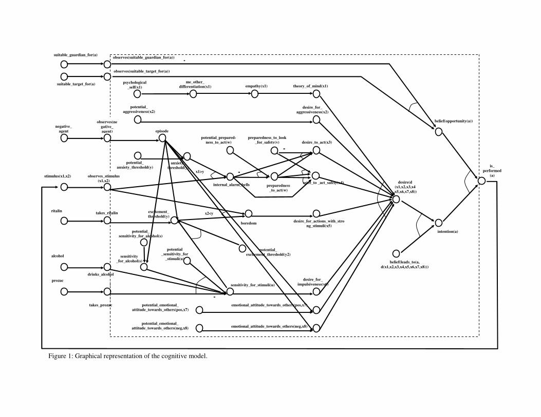
Figure 1: Graphical representation of the cognitive model.
potential_emotional_
attitude_towards_others(neg,x8)
-
suitable_target_for(a)
suitable_guardian_for(a)
observes(suitable_target_for(a))
observes(suitable_guardian_for(a))
belief(opportunity(a))
potential_
sensitivity_for_alcohol(s)
desire_for_
impulsiveness(x6)
anxiety_
threshold(y)
potential_
aggressiveness(x2)
-
potential_
anxiety_threshold(y)
desire_to _act_safely(x4)
desire_to_act(x3)
ritalin
sensitivity
_for_alcohol(s)
drinks_alcohol
desire(d
(x1,x2,x3,x4
,x5,x6,x7,x8))
emotional_attitude_towards_others(neg,x8)
emotional_attitude_towards_others(pos,x7)
-
boredom
desire_for_actions_with_stro
ng_stimuli(x5)
internal_alarm_bells
desire_for_
aggressiveness(x2)
-
theory_of_mind(x1)
empathy(x1)
me_other_
differentiation(x1)
psychological
_self(x1)
stimulus(x1,x2)
x2<y
alcohol
prozac
takes_ritalin
takes_prozac
excitement_
threshold(y)
observes_stimulus
(x1,x2)
-
potential_emotional_
attitude_towards_others(pos,x7)
sensitivity_for_stimuli(u)
potential
_sensitivity_for
_stimuli(u)
potential_
excitement_threshold(y2)
preparedness
_to_act(w)
preparedness_to_look
_for_safety(v)
x1>y
negative_
agent
observes(ne
gative_
agent) episode
potential_prepared-
ness_to_act(w)
-
belief(leads_to(a,
d(x1,x2,x3,x4,x5,x6,x7,x8)))
intention(a)
is_
performed
(a)
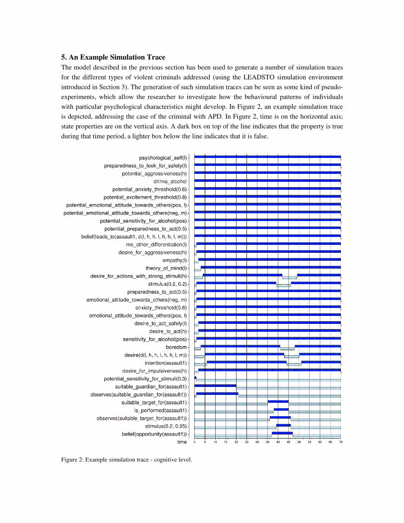
5. An Example Simulation Trace
The model described in the previous section has been used to generate a number of simulation traces
for the different types of violent criminals addressed (using the LEADSTO simulation environment
introduced in Section 3). The generation of such simulation traces can be seen as some kind of pseudo-
experiments, which allow the researcher to investigate how the behavioural patterns of individuals
with particular psychological characteristics might develop. In Figure 2, an example simulation trace
is depicted, addressing the case of the criminal with APD. In Figure 2, time is on the horizontal axis;
state properties are on the vertical axis. A dark box on top of the line indicates that the property is true
during that time period, a lighter box below the line indicates that it is false.
Figure 2: Example simulation trace - cognitive level.
The initial state properties that have been set to model the person with APD are (see time point 0):
low psychological self, low preparedness to look for safety, high potential aggressiveness, rather high
potential anxiety and excitement threshold (resp. value 0.6 and 0.8, on a [0,1] scale), potentially a low
positive and a medium negative emotional attitude towards others, a medium potential preparedness to
act (value 0.5), a low potential sensitivity for stimuli (value 0.3), and (s)he drinks alcohol and is
sensitive for it. These initial characteristics, combined with certain world stimuli, eventually lead to a
specific composed desire d(l, h, h, l, h, h, l, m) (see time point 5), characterised by the following
ingredients: low theory of mind, high aggressiveness, high desire to act, low desire to act safely, high
desire for actions with strong stimuli, high impulsiveness, low positive and medium negative
emotional attitude towards others. As a result, the criminal generates an intention to perform a specific
type of assault (denoted by assault1), and, as soon as the opportunity is there, actually performs the
assault. As a result, the stimuli as observed in the world increase, which satisfies the desires of the
criminal (at least temporarily).
6. The Approach to Reduction Used The psychological concepts used within Criminology to describe criminal behaviour are often
complex concepts for which it is not always easy to give a precise definition. It may even be argued
that for some of these concepts, there is a risk of circularity. For example, the internal state of
aggressiveness may be related to aggressive or violent behaviour1. To clarify such issues, it may be
worthwhile to have some reflection on how these concepts are embedded in reality. In (Bosse, Jonker
and Treur, 2006) three perspectives are put forward: (1) specification of functional roles, (2)
specification of representation relations, cf. (Kim, 1996), and (3) specification of realisation or
reduction relations. Here (1) is already covered by the LEADSTO properties of the simulation model.
Moreover, (2) can be obtained from these functional role specifications by determining their transitive
closure. This is not the focus of this paper; however, see for example, (Bosse, Jonker, Schut, and
Treur, 2006).
This paper focuses on the third way of grounding of the cognitive model. A mapping from the
cognitive concepts in this model to biological concepts will be established, thus obtaining a reduction
relation; more specifically, cognitive states will be mapped to anatomical, neurophysiological and
biochemical states, and cognitive dynamics to biological dynamics. Before this mapping is actually
applied (see Section 7), this section first provides a brief overview of different approaches to
reduction; a more extensive presentation of these approaches and their comparison can be found in
(Treur, 2011, Section 2).
Reduction relations have been addressed in a wide variety of publications in the philosophical and
logical literature; see, for example: (Balzer and Moulines, 1996; Bennett and Hacker, 2003; Bickle,
1998, 2003; Churchland, 1986; Hawkins and Kandel, 1984ab; Link, 2000; Kim, 1996, 1998, 2005;
Lewis, 1972, 1979; Nagel, 1961; Smart, 1959; Treur, 2011; Van Oudenhove and Cuypers, 2010).
In the classical approach, following Nagel (1961), reduction relations are based on (biconditional)
bridge principles a ↔ b that relate the expressions a in the language of a higher-level theory T2 (e.g., a
cognitive theory) to expressions b in the language of the lower-level theory T1 (e.g., a biological
theory). Kim (2005, pp. 98-102) calls Nagel’s approach bridge law reduction, as opposed to the type
of reduction he puts forward: functional reduction based on functionalisation of a target state property
1 A similar example is: “Opium puts people to sleep, because it contains a dormative principle” (Bateson, 1979).
a in T2 in terms of its causal task C, and relating it to a state property b in T1 performing this causal task
C. Also functional reduction is based on relationships between entities in the languages of the two
theories; however, these relationships are a bit less direct than biconditional bridge principles. From
the logical perspective two closely related notions to formalise reduction relations are (relative)
interpretation mappings (e.g., Tarski, Mostowski, and Robinson, 1953; Schoenfield, 1967, pp. 61-65;
Hodges, 1993, pp. 201-263; Niebergal, 2000; Feferman, 2000), and translations (e.g., Feferman, 2000;
Wang, 1951; Kreisel, 1955). These approaches relate the two theories T2 and T1 based on a mapping ϕ
relating syntactical elements a of T2 to syntactical elements b of T1, in the sense that b = ϕ(a). A type
of reduction relation not relating syntactical elements, but model structures is structural reduction;
e.g., Balzer and Moulines (1996). Using the structuralist perspective, Bickle (1998, pp. 199-211)
discusses revisionary (or new wave) reduction. Bickle (1998, pp. 205-208) illustrates this account for
the higher-level (folk psychological) and lower-level (neurobiological) explanation in the context of
memory consolidation; for further development, see Bickle (2003). The interpretation mapping
approach by (Tarski, Mostowski, and Robinson, 1953) will be taken as a focus in subsequent sections.
The basic idea of an interpretation of a theory T2 in a theory T1 is that an appropriate mapping ϕ
from the expressions of T2 to expressions of T1 is specified that satisfies the property that if an
expression or law L can be derived from T2, then ϕ(L) can be derived from T1:
T2 |─ L ⇒ T1 |─ ϕ(L)
An example of such an L is the statement that an aggressive state leads to aggressive behaviour.
Additional conditions on the mapping ϕ usually express that it is defined in an effective manner
and is compositional, i.e., that it preserves the compositional logical structure of the expression, for
example:
ϕ(a1 ∧ a2) = ϕ(a1) ∧ ϕ(a2)
ϕ(a1 → a2) = ϕ(a1) → ϕ(a2)
ϕ(¬ a) = ¬ ϕ(a)
These rules for preservation of compositional structure can be used to define an interpretation
mapping for more complex formulae in an inductive manner, taking the mapping of atoms as a point
of departure. Sometimes atoms are mapped as well according to their structure. For example, the
mapping of an atom R(f(x), g(y)) with relation symbol R, function symbols f and g and variables x and
y can be based on mappings between symbols R → R', f → f', g→ g', x → x', y → y' to obtain
ϕ(R(f(x), g(y))) = R'(f'(x'), g'(x'))
In such a way an interpretation mapping can be based on an ontology mapping, i.e., a mapping of the
different basic ontological elements used. For more details on interpretations, see, for example
(Tarski, Mostowski, and Robinson, 1953; Schoenfield, 1967, pp. 61-65 ; Hodges, 1993, pp. 201-263;
Feferman, 2000, pp. 84-87; Joosten and Visser, 2000, pp. 3-5; Niebergall, 2000, pp. 30-31).
In the next section, the specific reduction relations to ground the cognitive model for criminal
behaviour will be defined based on an interpretation mapping.
7. Mapping Cognitive to Biological States
In order to provide a grounding of the cognitive model, a mapping from cognitive concepts to
anatomical, neurophysiological and biochemical concepts will be established. Thus, reduction
relations are formalised by an interpretation mapping (as discussed in the previous section). In the
current section it is discussed how a conceptualisation based on cognitive state properties can formally
be mapped onto a conceptualisation based on biological state properties. As an example, the fact that
under certain circumstances states of impulsiveness and aggressiveness may lead to an impulsive,
violent crime (as described in the cognitive model) can also be described in terms of biological states
concerning high testosterone and low blood sugar. In the next section it is shown how this basic
mapping can be extended to an interpretation mapping for the dynamics.
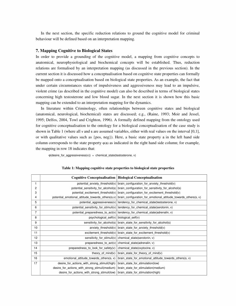
In literature within Criminology, often relationships between cognitive states and biological
(anatomical, neurological, biochemical) states are discussed; e.g., (Raine, 1993; Moir and Jessel,
1995; Delfos, 2004, Towl and Crighton, 1996). A formally defined mapping from the ontology used
for cognitive conceptualisation to the ontology for a biological conceptualisation of the case study is
shown in Table 1 (where all v and s are assumed variables, either with real values on the interval [0,1],
or with qualitative values such as {pos, neg}). Here, a basic state property a in the left hand side
column corresponds to the state property ϕ(a) as indicated in the right hand side column; for example,
the mapping in row 18 indicates that:
ϕ(desire_for_aggressiveness(v)) = chemical_state(testosterone, v)
Table 1: Mapping cognitive state properties to biological state properties
Cognitive Conceptualisation Biological Conceptualisation
1
2
3
4
potential_anxiety_threshold(v)
potential_sensitivity_for_alcohol(s)
potential_excitement_threshold(v)
potential_emotional_attitude_towards_others(s,v)
brain_configuration_for_anxiety_threshold(v)
brain_configuration_for_sensitivity_for_alcohol(s)
brain_configuration_for_excitement_threshold(v)
brain_configuration_for_emotional_attitude_towards_others(s, v)
5 potential_aggressiveness(v) tendency_for_chemical_state(testosterone, v)
6 potential_sensitivity_for_stimuli(v) tendency_for_chemical_state(serotonin, v)
7 potential_preparedness_to_act(v) tendency_for_chemical_state(adrenalin, v)
8 psychological_self(v) biological_self(v)
9 sensitivity_for_alcohol(s) brain_state_for_sensitivity_for_alcohol(s)
10 anxiety_threshold(v) brain_state_for_anxiety_threshold(v)
11 excitement_threshold(v) brain_state_for_excitement_threshold(v)
12 sensitivity_for_stimuli(v) chemical_state(serotonin, v)
13 preparedness_to_act(v) chemical_state(adrenalin, v)
14 preparedness_to_look_for_safety(v) chemical_state(oxytocine, v)
15 theory_of_mind(v) brain_state_for_theory_of_mind(v)
16 emotional_attitude_towards_others(s, v) brain_state_for_emotional_attitude_towards_others(s, v)
17 desire_for_actions_with_strong_stimuli(high)
desire_for_actions_with_strong_stimuli(medium)
desire_for_actions_with_strong_stimuli(low)
brain_state_for_stimulation(low)
brain_state_for_stimulation(medium)
brain_state_for_stimulation(high)

18 desire_for_aggressiveness(v) chemical_state(testosterone, v)
19 desire_to_act(v) chemical_state(adrenalin, v)
20 desire_to_act_safely(v) chemical_state(oxytocine, v)
21 desire_for_impulsiveness(v) chemical_state(bloodsugar, v)
22 desire(d(v1, v2, v3, v4, v5, v6, v7, v8)) biological_state(v1, v2, v3, v4, v5, v6, v7, v8)
23 episode brain_state_for_anxiety_threshold(high) &
brain_state_for_excitement_threshold(high) &
brain_state_for_sensitivity_for_alcohol(pos) &
brain_state_for_emotional_attitude_towards_others(pos, low) &
brain_state_for_emotional_attitude_towards_others(neg, low) &
The assumption behind the ontology mapping is that if b = ϕ(a), then b occurs if and only if a occurs.
Note that those concepts from Figure 1 that are not mentioned in Table 1 (e.g., negative_agent or
observes_stimulus) are mapped to the identical concept in the biological conceptualisation. The
mapping has been established on the basis of the information in, among others, (Raine, 1993; Moir
and Jessel, 1995; Delfos, 2004, Towl and Crighton, 1996).
Note that the mapping as presented above assumes that each concept in the cognitive model can be
mapped in a one-to-one manner to a concept in the biological model. For the moment, this assumption
is made, to keep the logical analysis manageable. Nevertheless, it might be more realistic to use a
probabilistic mapping, similar to methods often used in biology and biomedicine. In Section 9, it is
shown how the model can be extended in order to incorporate probabilistic mappings.
To give an impression of the type of information from the literature that the mapping is based on,
the mapping in row 13, stating that preparedness to act maps to the level of adrenalin, can be related to
the following quote by (Moir and Jessel, 1995):
“The more adrenaline in the blood and urine, the greater the stress we are reacting to.” (p. 75)
Similarly, the mapping in row 14, stating that preparedness to look for safety maps to the level of
oxytocine, can be related to the following quote by (Delfos, 2004):
“Women on the other hand have more the tendency to act by looking for safety and help in case of danger. Under
the influence of the hormone oxytocin, mainly produced by women, women are more likely to look after the nest,
the children or the household and talk to friends.” (p. 71)
Furthermore, the mapping in row 18, stating that desire for aggressiveness maps to the level of
testosterone, can be related to the following quote by (Delfos, 2004):
“Testosterone is also connected to aggression. Researchers like van der Dennen (1992) showed that to humans,
and also to animals, the fact applies that the higher the testosterone level, the more aggression is shown.” (p. 65)
As a final example, the mapping in row 23, about the biological background of episodes, can be
related to the following quote by (Moir and Jessel, 1995):
“Most of the people who demonstrated this condition were seemingly normal personalities, who would become
aggressive with very little reason. It would take only a mild trigger to produce this abnormal electrical discharge.
In a small but significant group of people who show explosively violent behaviour, the explosion comes from
within the brain, specifically from the limbic system and the amygdala (which control - in normal circumstances -
anger, hate and other emotional responses). What seems to be happening is that the brain itself generates a form of
miniature epileptic fit. An electric storm in the rage areas spreads to the rest of the brain, resulting in apparently
unprovoked, unfocused violence, including serious assault and particularly violent rape. (...) There is, however,
strong evidence that the tiniest amount of alcohol can set off the random electrical activity.” (p.187)
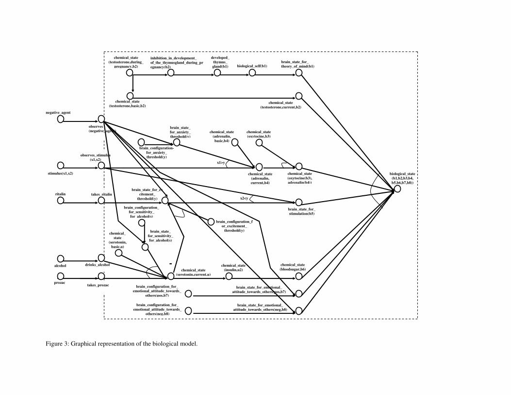
Figure 3: Graphical representation of the biological model.
chemical_
state
(serotonin,
basic,u)
developed_
thymus_
gland(b1)
brain_configuration-
for_anxiety_
threshold(y)
chemical_state
(oxytocine(b3),
adrenalin(b4))
ritalin
brain_state_
for_anxiety_
threshold(y)
biological_state
(b1,b2,b3,b4,
b5,b6,b7,b8))
brain_state_for_emotional_
attitude_towards_others(neg,b8)
brain_state_for_emotional_
attitude_towards_others(pos,b7)
-
brain_state_for_
stimulation(b5)
chemical_state
(testosterone,current,b2)
brain_state_for_
theory_of_mind(b1)
chemical_state
(testosterone,during_
pregnancy,b2)
x2<y
alcohol
prozac
x1>y
brain_state_for_ex
citement_
threshold(y)
brain_configuration_for_
emotional_attitude_towards_
others(pos,b7)
brain_configuration_for_
emotional_attitude_towards_
others(neg,b8)
chemical_state
(insulin,u2)
chemical_state
(bloodsugar,b6)
chemical_state
(adrenalin,
current,b4)
chemical_state
(oxytocine,b3)
inhibition_in_development_
of_the_thymusgland_during_pr
egnancy(b2)
biological_self(b1)
chemical_state
(testosterone,basic,b2)
observes_stimulus
(x1,x2)
stimulus(x1,x2)
takes_ritalin
chemical_state
(serotonin,current,u)
drinks_alcohol
takes_prozac
brain_state_
for_sensitivity_
for_alcohol(s)
brain_configuration_
for_sensitivity_
for_alcohol(s)
brain_configuration_f
or_excitement_
threshold(y)
-
chemical_state
(adrenalin,
basic,b4)
negative_agent
observes
(negative_agent)
In order to provide some more extensive support for these mappings, a complete overview of
literature references is given in Appendix B.
On the basis of this interpretation mapping, the concepts in the cognitive model (depicted in Figure
1) can be mapped onto concepts at a biological level, which have their own biological causal
relationships, as shown in Figure 3. Here, the circles again denote state properties, and the arrows
denote the causal relationships. For simplicity, the BDI-model that was shown at the right hand part of
Figure 1 has been left out of this picture.
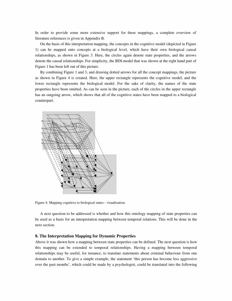
By combining Figure 1 and 3, and drawing dotted arrows for all the concept mappings, the picture
as shown in Figure 4 is created. Here, the upper rectangle represents the cognitive model, and the
lower rectangle represents the biological model. For the sake of clarity, the names of the state
properties have been omitted. As can be seen in the picture, each of the circles in the upper rectangle
has an outgoing arrow, which shows that all of the cognitive states have been mapped to a biological
counterpart.
Figure 4: Mapping cognitive to biological states - visualisation.
A next question to be addressed is whether and how this ontology mapping of state properties can
be used as a basis for an interpretation mapping between temporal relations. This will be done in the
next section.
8. The Interpretation Mapping for Dynamic Properties
Above it was shown how a mapping between state properties can be defined. The next question is how
this mapping can be extended to temporal relationships. Having a mapping between temporal
relationships may be useful, for instance, to translate statements about criminal behaviour from one
domain to another. To give a simple example, the statement ‘this person has become less aggressive
over the past months’, which could be made by a psychologist, could be translated into the following

statement in biological terms: ‘this person’s level of testosterone has decreased over the past months’.
This idea of mapping dynamic properties will be addressed in this section in the following sense:
• from a temporal relationship ψ expressed in the logical language TTL (Bosse, Jonker, Meij,
Sharpanskykh, and Treur, 2009), to a mapped temporal relationship ϕ(ψ)
• from a LEADSTO (Bosse, Jonker, Meij, and Treur, 2007) relationship α →→ β, to a LEADSTO
relationship ϕ(α →→ β)
8.1 Mapping a temporal relationship
First it is shown how the interpretation mapping for temporal relationships expressed in the dynamic
modelling language TTL can be defined. As explained earlier, expressions in TTL are predicate
logical formulae, built on basic atomic expressions of the form (1) state(γ, t) |= p, which indicates that
state property p holds in trace γ at time point t, or (2) value and time ordering relations. The cognitive
state property p can already be mapped onto ϕ(p) in the biological conceptualisation. Then the basic
expression state(γ, t) |= p is mapped as follows:
ϕ(state(γ, t) |= p) = state(γ, t) |= ϕ(p).
When α is an atom based on an equality or ordering relation, for example of the form v1 < v2, then
ϕ(v1 < v2) = v1 < v2.
After these TTL-atoms have been mapped, more complex TTL expressions as a whole can be mapped
in a straightforward compositional manner:
ϕ(A & B) = ϕ(A) & ϕ(B)
ϕ(A∨ B) = ϕ(A) ∨ ϕ(B)
ϕ(¬ A) = ¬ ϕ(A)
ϕ(A ⇒ B) = ϕ(A) ⇒ ϕ(B)
ϕ(∀v A(v)) = ∀v ϕ(A(v))
ϕ(∃v A(v)) = ∃v ϕ(A(v) )
An example mapping of a temporal relationship will be given in Section 10.
8.2 Mapping a LEADSTO relation
As explained in Section 3, LEADSTO is an executable sublanguage of TTL, which has specifically
been designed for the purpose of simulation. Hence, temporal LEADSTO relationships are a specific
type of relationships that can be defined within TTL. The mapping between temporal relationships in
general can be restricted to mapping of LEADSTO relationships as follows, where α and β are
conjunctions of literals. First define the expression α →→ β in terms of TTL:
∀γ ∀t1: [∀t [ t1 – g ≤ t < t1) ⇒ state(γ, t) |= α ] ⇒ ∃d ∈ [e, f] ∀t [ t1 + d ≤ t <t1 + d + h ⇒ state(γ, t) |= β ]
Then apply the mapping to this expression:
ϕ(α →→ β) =
ϕ(∀γ ∀t1: [∀t [ t1 – g ≤ t < t1) ⇒ state(γ, t) |= α ] ⇒
∃d ∈ [e, f] ∀t [ t1 + d ≤ t <t1 + d + h ⇒ state(γ, t) |= β ])
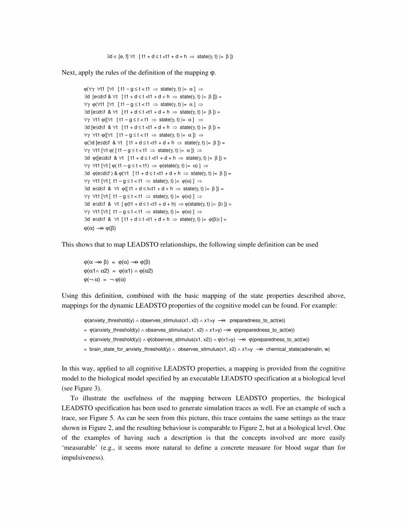
Next, apply the rules of the definition of the mapping ϕ.
ϕ(∀γ ∀t1 [∀t [ t1 – g ≤ t < t1 ⇒ state(γ, t) |= α ] ⇒
∃d [e≤d≤f & ∀t [ t1 + d ≤ t <t1 + d + h ⇒ state(γ, t) |= β ]]) =
∀γ ϕ(∀t1 [∀t [ t1 – g ≤ t < t1 ⇒ state(γ, t) |= α ] ⇒
∃d [e≤d≤f & ∀t [ t1 + d ≤ t <t1 + d + h ⇒ state(γ, t) |= β ]) =
∀γ ∀t1 ϕ([∀t [ t1 – g ≤ t < t1 ⇒ state(γ, t) |= α ] ⇒
∃d [e≤d≤f & ∀t [ t1 + d ≤ t <t1 + d + h ⇒ state(γ, t) |= β ]) =
∀γ ∀t1 ϕ([∀t [ t1 – g ≤ t < t1 ⇒ state(γ, t) |= α ]) ⇒
ϕ(∃d [e≤d≤f & ∀t [ t1 + d ≤ t <t1 + d + h ⇒ state(γ, t) |= β ]) =
∀γ ∀t1 [∀t ϕ( [ t1 – g ≤ t < t1 ⇒ state(γ, t) |= α ]) ⇒
∃d ϕ([e≤d≤f & ∀t [ t1 + d ≤ t <t1 + d + h ⇒ state(γ, t) |= β ]) =
∀γ ∀t1 [∀t [ ϕ( t1 – g ≤ t < t1) ⇒ ϕ(state(γ, t) |= α) ] ⇒
∃d ϕ(e≤d≤f ) & ϕ(∀t [ t1 + d ≤ t <t1 + d + h ⇒ state(γ, t) |= β ]) =
∀γ ∀t1 [∀t [ t1 – g ≤ t < t1 ⇒ state(γ, t) |= ϕ(α) ] ⇒
∃d e≤d≤f & ∀t ϕ([ t1 + d ≤ t<t1 + d + h ⇒ state(γ, t) |= β ]) =
∀γ ∀t1 [∀t [ t1 – g ≤ t < t1 ⇒ state(γ, t) |= ϕ(α) ] ⇒
∃d e≤d≤f & ∀t [ ϕ(t1 + d ≤ t <t1 + d + h) ⇒ ϕ(state(γ, t) |= β) ]) =
∀γ ∀t1 [∀t [ t1 – g ≤ t < t1 ⇒ state(γ, t) |= ϕ(α) ] ⇒
∃d e≤d≤f & ∀t [ t1 + d ≤ t <t1 + d + h ⇒ state(γ, t) |= ϕ(β)) ] =
ϕ(α) →→ ϕ(β)
This shows that to map LEADSTO relationships, the following simple definition can be used
ϕ(α →→ β) = ϕ(α) →→ ϕ(β)
ϕ(α1∧ α2) = ϕ(α1) ∧ ϕ(α2)
ϕ(¬ α) = ¬ ϕ(α)
Using this definition, combined with the basic mapping of the state properties described above,
mappings for the dynamic LEADSTO properties of the cognitive model can be found. For example:
ϕ(anxiety_threshold(y) ∧ observes_stimulus(x1, x2) ∧ x1>y →→ preparedness_to_act(w))
= ϕ(anxiety_threshold(y) ∧ observes_stimulus(x1, x2) ∧ x1>y) →→ ϕ(preparedness_to_act(w))
= ϕ(anxiety_threshold(y)) ∧ ϕ(observes_stimulus(x1, x2)) ∧ ϕ(x1>y) →→ ϕ(preparedness_to_act(w))
= brain_state_for_anxiety_threshold(y) ∧ observes_stimulus(x1, x2) ∧ x1>y →→ chemical_state(adrenalin, w)
In this way, applied to all cognitive LEADSTO properties, a mapping is provided from the cognitive
model to the biological model specified by an executable LEADSTO specification at a biological level
(see Figure 3).
To illustrate the usefulness of the mapping between LEADSTO properties, the biological
LEADSTO specification has been used to generate simulation traces as well. For an example of such a
trace, see Figure 5. As can be seen from this picture, this trace contains the same settings as the trace
shown in Figure 2, and the resulting behaviour is comparable to Figure 2, but at a biological level. One
of the examples of having such a description is that the concepts involved are more easily
‘measurable’ (e.g., it seems more natural to define a concrete measure for blood sugar than for
impulsiveness).
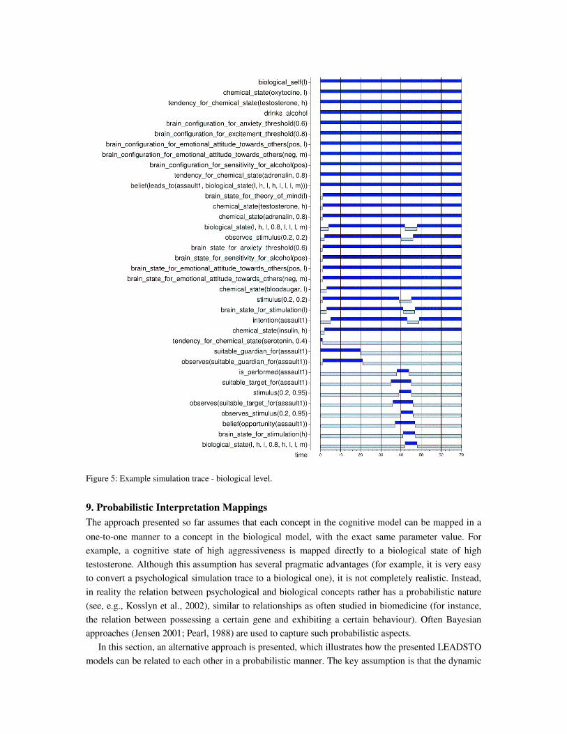
Figure 5: Example simulation trace - biological level.
9. Probabilistic Interpretation Mappings
The approach presented so far assumes that each concept in the cognitive model can be mapped in a
one-to-one manner to a concept in the biological model, with the exact same parameter value. For
example, a cognitive state of high aggressiveness is mapped directly to a biological state of high
testosterone. Although this assumption has several pragmatic advantages (for example, it is very easy
to convert a psychological simulation trace to a biological one), it is not completely realistic. Instead,
in reality the relation between psychological and biological concepts rather has a probabilistic nature
(see, e.g., Kosslyn et al., 2002), similar to relationships as often studied in biomedicine (for instance,
the relation between possessing a certain gene and exhibiting a certain behaviour). Often Bayesian
approaches (Jensen 2001; Pearl, 1988) are used to capture such probabilistic aspects.
In this section, an alternative approach is presented, which illustrates how the presented LEADSTO
models can be related to each other in a probabilistic manner. The key assumption is that the dynamic
models themselves (both the cognitive and the biological model) are still deterministic, but that the
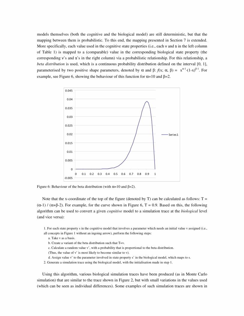
mapping between them is probabilistic. To this end, the mapping presented in Section 7 is extended.
More specifically, each value used in the cognitive state properties (i.e., each v and s in the left column
of Table 1) is mapped to a (comparable) value in the corresponding biological state property (the
corresponding v’s and s’s in the right column) via a probabilistic relationship. For this relationship, a
beta distribution is used, which is a continuous probability distribution defined on the interval [0, 1],
parameterised by two positive shape parameters, denoted by α and β: f(x; α, β) = xα-1
·(1-x)β-1
. For
example, see Figure 6, showing the behaviour of this function for α=10 and β=2.
-0.005
0
0.005
0.01
0.015
0.02
0.025
0.03
0.035
0.04
0.045
0 0.1 0.2 0.3 0.4 0.5 0.6 0.7 0.8 0.9 1
Series1
Figure 6: Behaviour of the beta distribution (with α=10 and β=2).
Note that the x-coordinate of the top of the figure (denoted by T) can be calculated as follows: T =
(α-1) / (α+β-2). For example, for the curve shown in Figure 6, T = 0.9. Based on this, the following
algorithm can be used to convert a given cognitive model to a simulation trace at the biological level
(and vice versa):
1. For each state property s in the cognitive model that involves a parameter which needs an initial value v assigned (i.e.,
all concepts in Figure 1 without an ingoing arrow), perform the following steps:
a. Take v as a basis.
b. Create a variant of the beta distribution such that T=v.
c. Calculate a random value v’, with a probability that is proportional to the beta distribution.
(Thus, the value of v’ is most likely to become similar to v).
d. Assign value v’ to the parameter involved in state property s’ in the biological model, which maps to s.
2. Generate a simulation trace using the biological model, with the initialisation made in step 1.
Using this algorithm, various biological simulation traces have been produced (as in Monte Carlo
simulation) that are similar to the trace shown in Figure 2, but with small variations in the values used
(which can be seen as individual differences). Some examples of such simulation traces are shown in
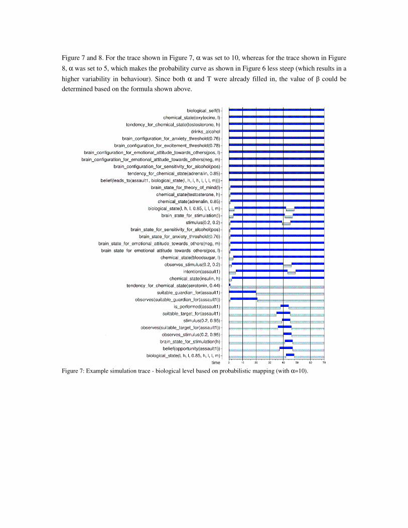
Figure 7 and 8. For the trace shown in Figure 7, α was set to 10, whereas for the trace shown in Figure
8, α was set to 5, which makes the probability curve as shown in Figure 6 less steep (which results in a
higher variability in behaviour). Since both α and T were already filled in, the value of β could be
determined based on the formula shown above.
Figure 7: Example simulation trace - biological level based on probabilistic mapping (with α=10).
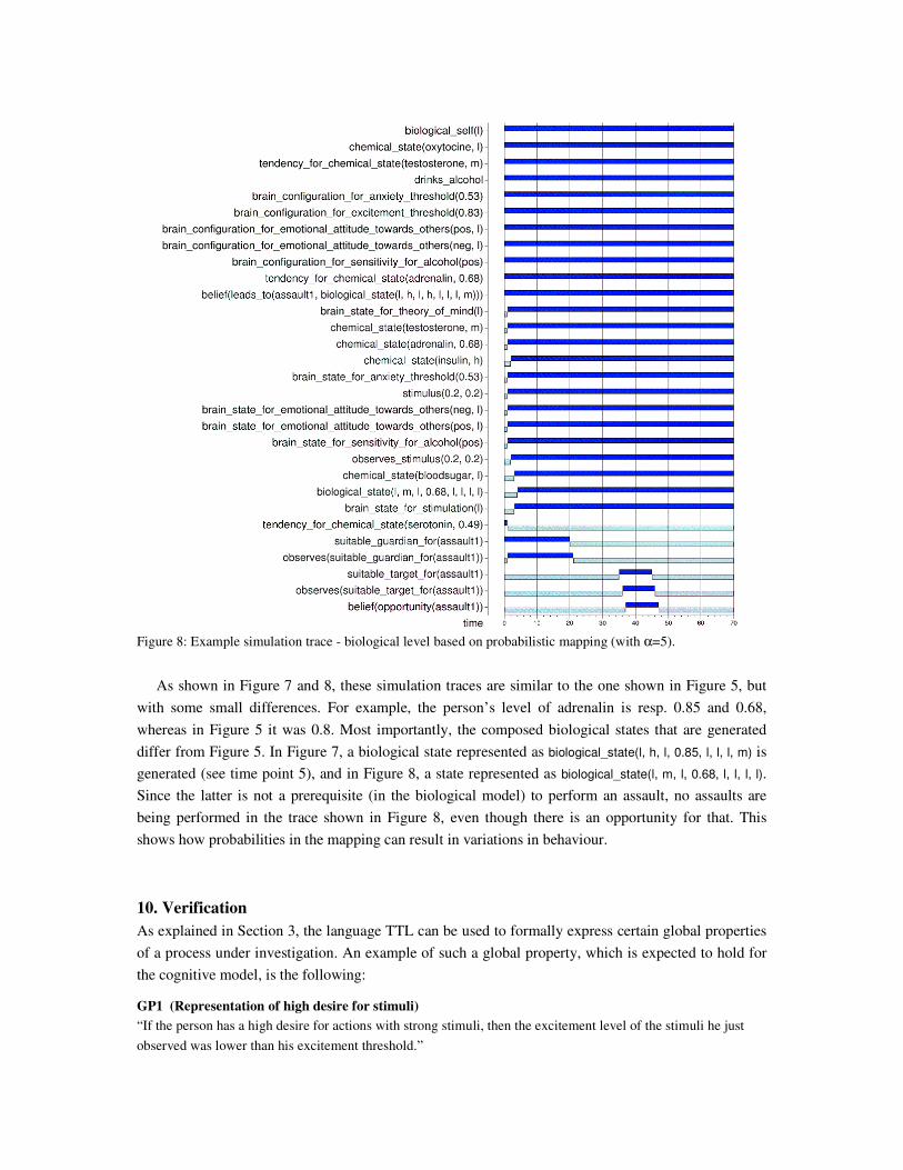
Figure 8: Example simulation trace - biological level based on probabilistic mapping (with α=5).
As shown in Figure 7 and 8, these simulation traces are similar to the one shown in Figure 5, but
with some small differences. For example, the person’s level of adrenalin is resp. 0.85 and 0.68,
whereas in Figure 5 it was 0.8. Most importantly, the composed biological states that are generated
differ from Figure 5. In Figure 7, a biological state represented as biological_state(l, h, l, 0.85, l, l, l, m) is
generated (see time point 5), and in Figure 8, a state represented as biological_state(l, m, l, 0.68, l, l, l, l).
Since the latter is not a prerequisite (in the biological model) to perform an assault, no assaults are
being performed in the trace shown in Figure 8, even though there is an opportunity for that. This
shows how probabilities in the mapping can result in variations in behaviour.
10. Verification
As explained in Section 3, the language TTL can be used to formally express certain global properties
of a process under investigation. An example of such a global property, which is expected to hold for
the cognitive model, is the following:
GP1 (Representation of high desire for stimuli)
“If the person has a high desire for actions with strong stimuli, then the excitement level of the stimuli he just
observed was lower than his excitement threshold.”
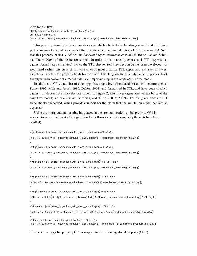
∀γ:TRACES ∀t:TIME
state(γ, t) |= desire_for_actions_with_strong_stimuli(high) ⇒
∃t’:TIME ∃x1,x2,y:REAL
[ t-d < t’ < t & state(γ, t’) |= observes_stimulus(x1,x2) & state(γ, t’) |= excitement_threshold(y) & x2<y ]
This property formulates the circumstances in which a high desire for strong stimuli is derived in a
precise manner (where d is a constant that specifies the maximum duration of desire generation). Note
that this property basically defines the backward representational content (cf. Bosse, Jonker, Schut,
and Treur, 2006) of the desire for stimuli. In order to automatically check such TTL expressions
against formal (e.g., simulated) traces, the TTL checker tool (see Section 3) has been developed. As
mentioned earlier, this piece of software takes as input a formal TTL expression and a set of traces,
and checks whether the property holds for the traces. Checking whether such dynamic properties about
the expected behaviour of a model hold is an important step in the verification of the model.
In addition to GP1, a number of other hypothesis have been formulated (based on literature such as
Raine, 1993; Moir and Jessel, 1995; Delfos, 2004) and formalised in TTL, and have been checked
against simulation traces like the one shown in Figure 2, which were generated on the basis of the
cognitive model; see also (Bosse, Gerritsen, and Treur, 2007a; 2007b). For the given traces, all of
these checks succeeded, which provides support for the claim that the simulation model behaves as
expected.
Using the interpretation mapping introduced in the previous section, global property GP1 is
mapped to an expression at a biological level as follows (where for simplicity the sorts have been
omitted):
ϕ(∀γ,t state(γ, t) |= desire_for_actions_with_strong_stimuli(high) ⇒ ∃t’,x1,x2,y
[ t-d < t’ < t & state(γ, t’) |= observes_stimulus(x1,x2) & state(γ, t’) |= excitement_threshold(y) & x2<y ])
=
∀γ,t ϕ(state(γ, t) |= desire_for_actions_with_strong_stimuli(high) ⇒ ∃t’,x1,x2,y
[ t-d < t’ < t & state(γ, t’) |= observes_stimulus(x1,x2) & state(γ, t’) |= excitement_threshold(y) & x2<y ])
=
∀γ,t ϕ(state(γ, t) |= desire_for_actions_with_strong_stimuli(high)) ⇒ ϕ(∃t’,x1,x2,y
[ t-d < t’ < t & state(γ, t’) |= observes_stimulus(x1,x2) & state(γ, t’) |= excitement_threshold(y) & x2<y ])
=
∀γ,t ϕ(state(γ, t) |= desire_for_actions_with_strong_stimuli(high)) ⇒ ∃t’,x1,x2,y
ϕ([ t-d < t’ < t & state(γ, t’) |= observes_stimulus(x1,x2) & state(γ, t’) |= excitement_threshold(y) & x2<y ])
=
∀γ,t ϕ(state(γ, t) |= desire_for_actions_with_strong_stimuli(high)) ⇒ ∃t’,x1,x2,y
[ ϕ(t-d < t’ < t) & ϕ(state(γ, t’) |= observes_stimulus(x1,x2)) & ϕ(state(γ, t’) |= excitement_threshold(y)) & ϕ(x2<y) ] =
∀γ,t state(γ, t) |= ϕ(desire_for_actions_with_strong_stimuli(high)) ⇒ ∃t’,x1,x2,y
[ ϕ(t-d < t’ < t) & state(γ, t’) |= ϕ(observes_stimulus(x1,x2)) & state(γ, t’) |= ϕ(excitement_threshold(y)) & ϕ(x2<y) ] =
∀γ,t state(γ, t) |= brain_state_for_stimulation(low) ⇒ ∃t’,x1,x2,y
[ t-d < t’ < t & state(γ, t’) |= observes_stimulus(x1,x2) & state(γ, t’) |= brain_state_for_excitement_threshold(y) & x2<y ]
Thus, eventually global property GP1 is mapped to the following global property (GP1’):
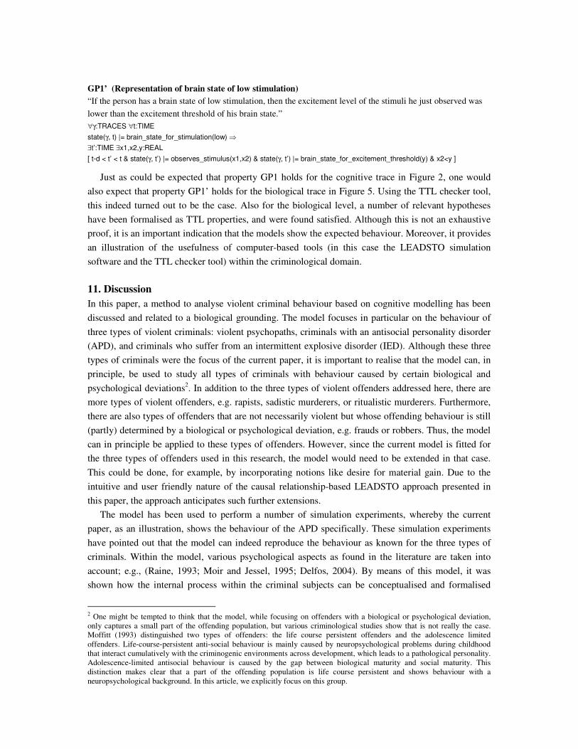
GP1’ (Representation of brain state of low stimulation)
“If the person has a brain state of low stimulation, then the excitement level of the stimuli he just observed was
lower than the excitement threshold of his brain state.”
∀γ:TRACES ∀t:TIME
state(γ, t) |= brain_state_for_stimulation(low) ⇒
∃t’:TIME ∃x1,x2,y:REAL
[ t-d < t’ < t & state(γ, t’) |= observes_stimulus(x1,x2) & state(γ, t’) |= brain_state_for_excitement_threshold(y) & x2<y ]
Just as could be expected that property GP1 holds for the cognitive trace in Figure 2, one would
also expect that property GP1’ holds for the biological trace in Figure 5. Using the TTL checker tool,
this indeed turned out to be the case. Also for the biological level, a number of relevant hypotheses
have been formalised as TTL properties, and were found satisfied. Although this is not an exhaustive
proof, it is an important indication that the models show the expected behaviour. Moreover, it provides
an illustration of the usefulness of computer-based tools (in this case the LEADSTO simulation
software and the TTL checker tool) within the criminological domain.
11. Discussion
In this paper, a method to analyse violent criminal behaviour based on cognitive modelling has been
discussed and related to a biological grounding. The model focuses in particular on the behaviour of
three types of violent criminals: violent psychopaths, criminals with an antisocial personality disorder
(APD), and criminals who suffer from an intermittent explosive disorder (IED). Although these three
types of criminals were the focus of the current paper, it is important to realise that the model can, in
principle, be used to study all types of criminals with behaviour caused by certain biological and
psychological deviations2. In addition to the three types of violent offenders addressed here, there are
more types of violent offenders, e.g. rapists, sadistic murderers, or ritualistic murderers. Furthermore,
there are also types of offenders that are not necessarily violent but whose offending behaviour is still
(partly) determined by a biological or psychological deviation, e.g. frauds or robbers. Thus, the model
can in principle be applied to these types of offenders. However, since the current model is fitted for
the three types of offenders used in this research, the model would need to be extended in that case.
This could be done, for example, by incorporating notions like desire for material gain. Due to the
intuitive and user friendly nature of the causal relationship-based LEADSTO approach presented in
this paper, the approach anticipates such further extensions.
The model has been used to perform a number of simulation experiments, whereby the current
paper, as an illustration, shows the behaviour of the APD specifically. These simulation experiments
have pointed out that the model can indeed reproduce the behaviour as known for the three types of
criminals. Within the model, various psychological aspects as found in the literature are taken into
account; e.g., (Raine, 1993; Moir and Jessel, 1995; Delfos, 2004). By means of this model, it was
shown how the internal process within the criminal subjects can be conceptualised and formalised
2 One might be tempted to think that the model, while focusing on offenders with a biological or psychological deviation,
only captures a small part of the offending population, but various criminological studies show that is not really the case.
Moffitt (1993) distinguished two types of offenders: the life course persistent offenders and the adolescence limited
offenders. Life-course-persistent anti-social behaviour is mainly caused by neuropsychological problems during childhood
that interact cumulatively with the criminogenic environments across development, which leads to a pathological personality.
Adolescence-limited antisocial behaviour is caused by the gap between biological maturity and social maturity. This
distinction makes clear that a part of the offending population is life course persistent and shows behaviour with a
neuropsychological background. In this article, we explicitly focus on this group.
from a cognitive perspective. However, as a main contribution, it was also shown how this model can
be biologically grounded. To this end it was shown how an ontological mapping from the cognitive
model to a biological formalisation can be formally defined. For example, the fact that under certain
circumstances states of impulsiveness and aggressiveness may lead to an impulsive, violent crime (as
described in the cognitive model) can be described in terms of biological states concerning high
testosterone and low blood sugar. It has been shown in detail how ontology elements for such
psychological states can be formally mapped onto ontology elements for biological states. Moreover,
this formal ontology mapping has been extended to a formal mapping of temporal dynamic properties.
Thus it is shown how the process description at the cognitive level relates to a process description at
the biological level. Finally, it was shown how the mapping can be extended in order to incorporate
probabilistic aspects. Having a mapping as described above allows one on the one hand to explain
behaviour in terms of psychological concepts, but on the other hand to relate it to a biological
grounding. Most of these steps have been supported by automated tools for simulation (Bosse, Jonker,
Meij, and Treur, 2007) and verification of properties (Bosse, Jonker, Meij, Sharpanskykh, and Treur,
2007).
Note that in the approach followed in this paper it is assumed that both the dynamical models at the
biological and at the psychological level are deterministic. The probabilistic element is concentrated
on the relation between biological and psychological states. Further research may also consider the
case that both dynamical models are probabilistic as well, and, for example, can be described by
Bayesian networks (Jensen 2001; Pearl, 1988). As also the mapping is considered to have a
probabilistic nature, and this has to be combined with the probabilistic aspects of each of the models,
such a step would entail an interesting but far from trivial challenge; it is left for future work.
As mentioned in the introduction, dynamic models for criminal behaviour as presented in this paper
are very useful for case analysis, i.e., given a certain crime case, to find out which type of person has
performed this crime (see also Bosse, Gerritsen, and Treur, 2007a). Following this idea, the current
paper is part of a larger project, involving researchers from Artificial Intelligence, Criminology, and
Psychology, which has as ultimate goal to develop an application that can assist police analysts in
solving crime cases. The main idea is that such a system takes several characteristics of a crime as
input (e.g. a time line of events, and characteristics of the criminal act, such as levels of aggressiveness
and impulsiveness), and is able to help the analyst in his or her reasoning process. This can be done,
for example, by generating simulations (or fictive scenarios), and matching these with the information
known from the real scenario, or by ruling out certain possible scenarios by using argumentation
techniques (cf. Bex et al., 2007). The current paper contributes a small step to that project, by
establishing a tighter connection between biological and psychological characteristics of offenders.
This is an important contribution, since the gap between biological descriptions of a criminal’s
behaviour (e.g., obtained by biological and sensor measurements) and the corresponding
psychological/cognitive descriptions (as often used by police analysts) is traditionally quite big. The
approach presented in this paper allows the user to reason about criminal behaviour on a psychological
level, but in the meantime relate this to a (up to a certain point) similar description on a biological
level, based on information which can actually be measured in the physical world.
Obviously, in order to develop a system that can actually be applied, more validation is needed. In
principle, validation can address both the dynamics of the cognitive model and the dynamics of the
underlying biological model. Moreover, the mapping between the cognitive and the underlying
biological model can be validated. In this paper, all of the mappings have been validated positively
against literature on the specific types of criminals addressed. Also the resulting mappings have been
discussed with our partners in criminology and psychology. In the future, we envision performing a
more ‘external’ validation, using real measurements. Some initial steps in that direction have been
made in (Both et al., 2009).
Acknowledgements
The authors are grateful to the anonymous reviewers for their useful feedback on an earlier version of
this article.
References
Baal, P.H.M. van (2004). Computer Simulations of Criminal Deterence: from Public Policy to Local Interaction
to Individual Behaviour. Ph.D. Thesis, Erasmus University Rotterdam. Boom Juridische Uitgevers.
Balzer, W., and Moulines, C.U. (1996). Structuralist Theory of Science. Walter de Gruyter, Berlin.
Baron-Cohen, S. (1995). Mindblindness. MIT Press.
Bartol, C.R. (2002). Criminal Behavior: a Psychosocial Approach. Sixth edition. Prentice Hall, New Jersey.
Bateson, G. (1979). Mind and Nature: A Necessary Unity. E. P. Dutton, New York.
Bennett, M. R., and Hacker, P. M. S. (2003). Philosophical foundations of neuroscience. Malden, MA:
Blackwell.
Bex, F.J., Braak, S.W. van den, Oostendorp, H. van, Prakken, H., Verheij, B. and Vreeswijk, G.A.W. (2007).
Sense-making software for crime investigation: how to combine stories and arguments? Law, Probablity and
Risk, 6(1-4), 145-168.
Bickle, J. (1998). Psychoneural Reduction: The New Wave. MIT Press, Cambridge, Massachusetts.
Bickle, J. (2003). Philosophy and Neuroscience: A Ruthless Reductive Account. Kluwer Academic Publishers.
Blair, R.J.R. (2005). Responding to the emotions of others: Dissociating forms of empathy through the study of
typical and psychiatric populations. Consciousness and Cognition, 14 (2005), pp. 698-718.
Bosse, T., Gerritsen, C., and Treur, J. (2007a). Case Analysis of Criminal Behaviour. In: Okuno H.G., and Ali,
M. (eds.), New Trends in Applied Artificial Intelligence, Proceedings of the 20th International Conference on
Industrial, Engineering and Other Applications of Applied Intelligent Systems, IEA/AIE’07. Lecture Notes in
Artificial Intelligence, vol. 4570. Springer Verlag, 2007, pp. 166-175.
Bosse, T., Gerritsen, C., and Treur, J. (2007b). Cognitive and Social Simulation of Criminal Behaviour: the
Intermittent Explosive Disorder Case. In: O. Shehory, M. Huhns (eds.), Proceedings of the Sixth International
Joint Conference on Autonomous Agents and Multi-Agent Systems, AAMAS'07. ACM Press, 2007, pp. 367-
374.
Bosse, T., Jonker, C.M., Meij, L. van der, Sharpanskykh, A., and Treur, J. (2009). Specification and Verification
of Dynamics in Agent Models. International Journal of Cooperative Information Systems, vol. 18, 2009, pp.
167 - 193. Shorter version in: Nishida, T. et al (eds.), Proc. of the 6th Int. Conf. on Intelligent Agent
Technology, IAT'06. IEEE Computer Society Press, 2006, pp.247-254.
Bosse, T., Jonker, C.M., Meij, L. van der, and Treur, J. (2007). A Language and Environment for Analysis of
Dynamics by Simulation. International Journal of Artificial Intelligence Tools, vol. 16, 2007, pp. 435-464.
Bosse, T., Jonker, C.M., Schut, M.C., and Treur, J. (2006). Collective Representational Content for Shared
Extended Mind. Cognitive Systems Research Journal, volume 7, issue 2-3, 2006, pp. 151-174.
Bosse, T., Jonker, C.M., and Treur, J. (2006). Developing Higher-Level Cognitive Theories by Reduction. In: R.
Sun, N. Miyake (eds.), Proc. of the 28th Annual Conference of the Cognitive Science Society, CogSci'06,
2006, pp. 1032-1037.

Both, F., Hoogendoorn, M., Lambalgen, R.M. van, Oorburg, R., and Vos, M. de (2009). Relating Personality and
Physiological Measurements to Task Performance Quality. In: Proceedings of the 31th Annual Conference of
the Cognitive Science Society, CogSci’09. Cognitive Science Society, Austin, TX, 2009.
Brantingham, P. L., & Brantingham, P. J. (2004). Computer Simulation as a Tool for Environmental
Criminologists. Security Journal, 17(1), 21-30.
Chan, H.C., Heide, K.M., and Beauregard, E. (2010). What Propels Sexual Murderers: A Proposed Integrated
Theoryof Social Learningand Routine Activities Theories. International Journal ofOffender Therapy and
Comparative Criminology. In Press. doi: 10.1177/0306624X10361317.
Churchland, P.S. (1986). Neurophilosophy: Toward a Unified Science of the Mind/Brain. MIT Press,
Cambridge, MA.
Cohen, L.E. and Felson, M. (1979). Social change and crime rate trends: a routine activity approach. American
Sociological Review, vol. 44, pp. 588-608.
Cornish, D.B., and Clarke, R.V. (1986). The Reasoning Criminal: Rational Choice Perspectives on Offending.
Springer Verlag.
Delfos, M.F. (2004). Children and Behavioural Problems: Anxiety, Aggression, Depression and ADHD; A
Biopsychological Model with Guidelines for Diagnostics and Treatment. Harcourt book publishers,
Amsterdam.
Dennett, D.C. (1987). The Intentional Stance. MIT Press. Cambridge Mass.
Feferman, S. (2000). Does Reductive Proof Theory Have a Viable Rationale? Erkenntnis: an International
Journal of Analytic Philosophy, vol. 53, pp. 63-96.
Felson, M. (2010). What every mathematician should know about modelling crime. Euro. Jnl of Applied
Mathematics (2010), vol. 21, pp. 275–281. doi:10.1017/S0956792510000070
Georgeff, M. P., and Lansky, A. L. (1987). Reactive Reasoning and Planning. In: Proceedings of the Sixth
National Conference on Artificial Intelligence, AAAI’87. Menlo Park, California. American Association for
AI, 1987, pp. 677-682.
Gottfredson, M., and Hirschi, T. (1990). A General Theory of Crime. Stanford University Press.
Hawkins, R.D., and Kandel, E.R. (1984a). Is There a Cell-Biological Alphabet for Simple Forms of Learning?
Psychological Review, vol. 91, pp. 375-391
Hawkins, R.D., and Kandel, E.R. (1984b). Steps Toward a Cell-Biological Alphabet for Elementary Forms of
Learning. In: G. Lynch, J.L. McGaugh, and N.M. Weinberger (eds.), Neurobiology of Learning and Memory,
Guilford Press, New York, pp. 385-404, vol. 91, pp. 375-391
Hodges, W. (1993). Model theory. Cambridge University Press.
Humphrey, N. (1984). Consciousness Regained. Oxford University Press.
Hutchings, A., and Hayes, H. (2009). Routine Activity Theory and Phishing Victimisation: Who Gets Caught in
the ‘Net’? Current Issues In Criminal Justice, vol. 20, pp. 433-451
Jensen, F.V. (2001). Bayesian Networks and Decision Graphs. Springer Verlag.
Jonker, C.M., Treur, J., and Wijngaards, W.C.A., (2003). A Temporal Modelling Environment for Internally
Grounded Beliefs, Desires and Intentions. Cognitive Systems Research Journal, vol. 4(3), 2003, pp. 191-210.
Joosten, J.J., and Visser, A. (2000). The interpretability logic of all reasonable arithmetical theories. The new
conjecture. Erkenntnis: an International Journal of Analytic Philosophy, vol. 53, pp. 3-26.
Kim, J. (1996). Philosophy of Mind, Westview Press.
Kim, J. (1998). Mind in a Physical world: an Essay on the Mind-Body Problem and Mental Causation. MIT
Press, Cambridge, Mass.
Kim, J. (2005). Physicalism, or Something Near Enough. Princeton University Press, Princeton.
Kosslyn, S.M., Cacioppo, J.T., Davidson, R.J., Hugdahl, K., Lovallo, W.R., Spiegel, D., and Rose, R. (2002).
Bridging psychology and biology. The analysis of individuals in groups. Am. Psychologist 2002, vol. 57, pp.
341-51.
Kreisel, G. (1955). Models, translations and Interpretations. In: Skolem, Th. Al. (eds.), Mathematical
Interpretation of Formal Systems. North-Holland, Amsterdam, pp. 26-50.
Lee, J., and Yu, C. (2010). The Development of Urban Crime Simulator. In: Proceedings of the 1st International
Conference and Exhibition on Computing for Geospatial Research & Application, COM.Geo’10. ACM Press.
Lewis, D.K. (1972). Psychophysical and Theoretical Identifications. Australasian Journal of Philosophy, vol. 50,
pp 249-258. Reprinted in Chung-ying Cheng, Ch.-Y (ed.) (1975), Philosophical Aspects of the Mind-Body
Problem (U.P. of Hawaii), and in Block, N. (ed.) (1980). Readings in the Philosophy of Psychology Volume I
(Harvard U.P.).
Lewis, D.K. (1979). How to Define Theoretical Terms. Journal of Philosophy, vol. 67, pp 427-446
Link, G. (ed.) (2000), Concepts of Reduction in Logic and Philosophy. Erkenntnis: an International Journal of
Analytic Philosophy, vol. 53 (no 1 and 2), pp. 1-283.
Liu, L., Wang, X., Eck, J., & Liang, J. (2005). Simulating Crime Events and Crime Patterns in RA/CA Model. In
F. Wang (ed.), Geographic Information Systems and Crime Analysis. Singapore: Idea Group, pp. 197-213
Marcum, C.D., Ricketts, M.L., and Higgins, G.E. (2010). Assessing Sex Experiences of Online Victimization:
An Examination of Adolescent Online Behaviors Using Routine Activity Theory. Criminal Justice Review, in
press, 2010. DOI: 10.1177/0734016809360331
Melo, A., Belchior, M., and Furtado, V. (2005). Analyzing Police Patrol Routes by Simulating the Physical
Reorganisation of Agents. In: Sichman, J.S., and Antunes, L. (eds.), Proceedings of the Sixth International
Workshop on Multi-Agent-Based Simulation, MABS'05. Lecture Notes in Artificial Intelligence, vol. 3891,
Springer Verlag, 2006, pp 99-114.
Moffitt, T.E. (1993). Adolescence-Limited and Life-Course-Persistent Antisocial Behavior: A Developmental
Taxonomy. Psychological Review, 100(4), pp. 674-701.
Moir, A., and Jessel, D. (1995). A Mind to Crime: the controversial link between the mind and criminal
behaviour. London: Michael Joseph Ltd; Penguin.
Nagel, E. (1961). The Structure of Science. London: Routledge & Kegan Paul.
Niebergall, K.-G. (2000), On the Logic of Reducibility: Axioms and Examples. Erkenntnis: an International
Journal of Analytic Philosophy, vol. 53, pp. 27-61.
Pearl, J. (1988). Probabilistic Reasoning in Intelligent Systems. Morgan Kaufmann.
Popp, A.M., and Peguero, A.A. (2010). Routine Activities and Victimization at School: The Significance of
Gender. Journal of Interpersonal Violence, 2010, in press. DOI: 10.1177/0886260510383021.
Pratt, T.C., Holtfreter, K., and Reisig, M.D. (2010). Routine Online Activity and Internet Fraud Targeting:
Extending the Generality of Routine Activity Theory. Journal of Research in Crime and Delinquency, vol.
47(3), pp. 267-296. DOI: 10.1177/0022427810365903.
Raine, A. (1993). The Psychopathology of Crime: Criminal Behaviors as a Clinical Disorder. New York, NY:
Guilford Publications.
Ramsey, F.P. (1929). Theories. Published in: Ramsey, F.P. (1931) The Foundations of Mathematics and Other
Essays (edited by R. B. Braithwaite), London: Routledge and Kegan Paul.
Rao, A.S. & Georgeff, M.P. (1991). Modelling Rational Agents within a BDI-architecture. In: Allen, J., Fikes, R.
and Sandewall, E. (eds.), Proceedings of the Second International Conference on Principles of Knowledge
Representation and Reasoning, (KR’91). Morgan Kaufmann, pp. 473-484.
Sampson, R., Eck, J.E., and Dunham, J. (2010). Super controllers and crime prevention: A routine activity
explanation of crime prevention success and failure. Security Journal , vol. 23, 2010, pp. 37–51
Schoenfield, J.R. (1967). Mathematical Logic. Addison-Wesley.
Smart, J.J.C. (1959). Sensations and Brain Processes. Philosophical Review, vol. 68, pp. 141-156. Reprinted in
Rosenthal, D.M. (ed.), The Nature of Mind. Oxford University Press, Oxford, 1991.
Tarski, A., Mostowski, A., and Robinson, R.M. (1953). Undecidable Theories. North-Holland, Amsterdam.
Towl, G.J., and Crighton, D.A. (1996). The Handbook of Psychology for Forensic Practitioners. Routledge,
London, New York.
Treur, J., (2011). On the Use of Reduction Relations to Relate Different Types of Agent Models. Web
Intelligence and Agent Systems Journal, 2011, vol. 9, in press.
Turvey, B. (1999). Criminal Profiling: an Introduction to Behavioral Evidence Analysis. Academic Press.
Van Oudenhove, L., and Cuypers, S.E. (2010). The Philosophical "Mind-Body Problem" and Its Relevance for
the Relationship Between Psychiatry and the Neurosciences. Perspectives in Biology and Medicine, vol. 53,
2010, pp. 545-557. DOI: 10.1353/pbm.2010.0012
Wang, H. (1951). Arithmetic Translations of Axiom Systems. Transactions American Math. Soc., vol. 71, pp.
283-293.
Webster, C.D., and M.A. Jackson (eds.), (1997). Impulsivity: Theory, Assessment and Treatment. Guilford, New
York.
Appendix A - The LEADSTO Simulation Model
All local properties (LP’s) that have been used for the simulation model are provided below in textual
form, both in an informal notation and in a formal (LEADSTO) notation. Many of these properties are
based on theories and experiments presented in the literature on criminal behaviour. References are
given to be able to trace back this source material. Note that some of the formulae and their specific
values (e.g., the value of 10 in LP20b) have been estimated in order to get an effect as qualitatively
described in the literature, rather than that they are known from this literature. However, if more
biological knowledge becomes available, such values can be validated and, if needed, easily be
incorporated in an improved form in the approach. The model consists of the following sub-models:
1. a model to determine actions based on beliefs, desires and intentions (BDI-model)
2. a model to determine desires used as input by the BDI-model
3. a model to determine beliefs in an opportunity as input for the BDI-model
A.1 The BDI-Submodel
LP1 A certain desire combined with the belief that a certain action will lead to the fulfillment of that desire leads to
an intention for that action.
(Rao and Georgeff, 1991) ∀x1,x2,x3,x4,x5,x6,x7,x8:SCALE ∀a:ACTION
desire(d(x1, x2, x3, x4, x5, x6, x7, x8)) ∧ belief (leads_to(a,d(x1, x2, x3, x4, x5, x6, x7, x8))) →→ intention(a)
LP2 The belief that there is an opportunity for a certain action combined with the intention to perform that action
leads to the performance of that action.
(Cohen, 1979; Rao and Georgeff, 1991) ∀a:ACTION
belief(opportunity(a)) ∧ intention(a) →→ is_performed(a)
A.2 The Submodel to Determine Desires
Development of a Theory of Mind
LP3 A certain level of psychological self leads to the same level of me-other differentiation.
(Delfos, 2004, p.56) ∀x:SCALE
psychological_self(x) →→ me_other_differentiation(x)
LP4 A certain level of me-other differentiation leads to the same level of empathy.
(Delfos, 2004, p.57) ∀x:SCALE
me_other_differentiation(x) →→ empathy(x)
LP5 A certain level of empathy leads to the same level of theory of mind.
(Delfos, 2004, p.59) ∀x:SCALE
empathy(x) →→ theory_of_mind(x)
Development of Aggressiveness
LP6 ∀x:SCALE A certain potential aggressiveness leads to the same level of desire for aggressiveness.
(Delfos, 2004, p.65, p.68, pp.83-85, p.112)
potential_aggressiveness(x) →→ desire_for_aggressiveness(x)
Development of Desires to Act (with and without Safety)
LP7a A potential anxiety threshold combined with an episode leads to an increased anxiety threshold.
(Moir and Jessel, 1995, pp.184-188) ∀y:REAL potential_anxiety_threshold(y) ∧ episode →→ anxiety_threshold(y+0.4*(1-y))
LP7b
A potential anxiety threshold not combined with an episode leads to the same anxiety threshold.
(Moir and Jessel, 1995, pp. 184-187; Raine, 1993, pp.169-173) ∀y:REAL
potential_anxiety_threshold(y) ∧ not episode →→ anxiety_threshold(y)
LP8
When you observe a stimulus that is higher than your anxiety threshold then internal alarm bells will go off.
(Delfos, 2004, p.69; Moir and Jessel, 1995, pp.75-76; Raine, 1993, p.166, p.179, p.222) ∀x1,x2,y:REAL
observes_stimulus(x1, x2) ∧ anxiety_threshold(y) ∧ x1>y →→ internal_alarm_bells
LP9a
Internal alarm bells increase the preparedness to act.
(Moir and Jessel, 1995, pp.75-76) ∀x:REAL internal_alarm_bells ∧ potential_preparedness_to_act(x) →→ preparedness_to_act(x+0.3*(1-x))
LP9b
In the absence of internal alarm bells, a certain level of potential preparedness to act leads to the same level of
preparedness to act. ∀x:REAL
preparedness_to_act(x) ∧ not internal_alarm_bells →→ preparedness_to_act(x)

LP10a
When you have a high preparedness to act and a high preparedness to look for safety then you will have a high
desire to act and a high desire to act safely. ∀x:REAL
preparedness_to_act(x) ∧ preparedness_to_look_for_safety(high) ∧ x ≥ 0.5 →→ desire_to_act(high) ∧ desire_to_act_safely(high)
LP10b When you have a high preparedness to act and there are internal alarm bells then you will have a high desire to
act and a high desire to act safely. ∀x:REAL
preparedness_to_act(x) ∧ internal_alarm_bells ∧ x ≥ 0.5 →→ desire_to_act(high) ∧ desire_to_act_safely(high)
LP10c When you have a high preparedness to act and a low preparedness to look for safety and there are no internal
alarm bells then you will have a high desire to act but a low desire to act safely. ∀x:REAL
preparedness_to_act(x) ∧ preparedness_to_look_for_safety(low) ∧ not internal_alarm_bells ∧ x ≥ 0.5 →→ desire_to_act(high) ∧ desire_to_act_safely(low)
LP11
When you have a low preparedness to act then you will have a low desire to act and a low desire to act safely. ∀x:REAL
preparedness_to_act(x) ∧ x < 0.5 →→ desire_to_act(low) ∧ desire_to_act_safely(low)
Development of Desires for Actions with Strong Stimuli
LP12a A sensitivity for stimuli of z and a potential excitement threshold of y not combined with an episode lead to an
excitement threshold of y+0.3*(1-(y-z))-z.
(Moir and Jessel, 1995, p.188, pp.202-204; Raine, 1993, pp.178-180, pp.222-228) ∀y:REAL ∀z:SIGN
sensitivity_for_stimuli(z) ∧ potential_excitement_threshold(y) ∧ not episode →→ excitement_threshold(y+0.3*(1-(y-z))-z)
LP12b A sensitivity for stimuli of z and a potential excitement threshold of y combined with an episode lead to an
excitement threshold of y+0.5*(1-(y-z))-z.
(Moir and Jessel, 1995, pp.184-188) ∀y:REAL ∀z:SIGN sensitivity_for_stimuli(z) ∧ potential_excitement_threshold(y) ∧ episode →→ excitement_threshold(y+0.5*(1-(y-z))-z)
LP13
Taking Ritalin decreases the excitement threshold.
(Moir and Jessel, 1995, p.80) ∀y:REAL takes_ritalin ∧ excitement_threshold(y) →→ excitement_threshold(y-0.1*y)
LP14
When you observe a stimulus that is lower than your excitement threshold than you will be bored.
(Delfos, 2004, p.100; Moir and jessel, 1995, p.173; Raine, 1993, pp.222-224) ∀x1,x2,y:REAL
observes_stimulus(x1,x2) ∧ excitement_threshold(y) ∧ x2<y →→ boredom
LP15
Boredom leads to a high desire for actions with strong stimuli.
(Delfos, 2004, p.100; Moir and Jessel, 1995, pp.74-80, pp.173-174)
boredom →→ desire_for_actions_with_strong_stimuli(high)
Development of Desires for Impulsiveness
LP16 A certain potential sensitivity for alcohol leads to the same sensitivity for alcohol.
(Moir and Jessel, 1995, pp.201-204, p.264; Raine, 1993, p.98, p.210) ∀s:SIGN potential_sensitivity_for_alcohol(s) →→ sensitivity_for_alcohol(s)
LP17a
Sensitivity for alcohol combined with an episode leads to positive sensitivity for alcohol.
(Moir and Jessel, 1995, pp.184-188) ∀s1:SIGN
sensitivity_for_alcohol(s1) ∧ episode →→ sensitivity_for_alcohol(pos)
LP17b A certain level of sensitivity for alcohol not combined with an episode remains the same. ∀s1:SIGN
sensitivity_for_alcohol(s1) ∧ not episode →→ sensitivity_for_alcohol(s1)
LP18 A potential sensitivity for stimuli leads to the same sensitivity for stimuli. ∀x:REAL potential_for_sensitivity_for_stimuli(x) →→ sensitivity_for_stimuli(x)
LP19a A negative sensitivity for alcohol combined with no alcohol and no prozac will lead to the same sensitivity for
stimuli.
(Moir and Jessel, 1995, p.71) ∀x:REAL
sensitivity_for_alcohol(neg) ∧ not drinks_alcohol ∧ sensitivity_for_stimuli(x) ∧ not takes_prozac →→0, 0, 1, 1 sensitivity_for_stimuli(x)
LP19b A negative sensitivity for alcohol combined with no alcohol and prozac will increase the sensitivity for stimuli
by 0.1.
(Moir and Jessel, 1995, p.71) ∀x:REAL
sensitivity_for_alcohol(neg) ∧ not drinks_alcohol ∧ sensitivity_for_stimuli(x) ∧ takes_prozac →→0, 0, 1, 1 sensitivity_for_stimuli(x+0.1*(1-x))
LP19c A negative sensitivity for alcohol combined with alcohol and no prozac will decrease the sensitivity for stimuli
by 0.1.
(Moir and Jessel, 1995, p.71) ∀x:REAL
sensitivity_for_alcohol(neg) ∧ drinks_alcohol ∧ sensitivity_for_stimuli(x) ∧ not takes_prozac →→0, 0, 1, 1 sensitivity_for_stimuli(x-0.1*x)
LP19d A negative sensitivity for alcohol combined with alcohol and prozac will lead to the same sensitivity for stimuli.
(Moir and Jessel, 1995, p.71) ∀x:REAL
sensitivity_for_alcohol(neg) ∧ drinks_alcohol ∧ sensitivity_for_stimuli(x) ∧ takes_prozac →→0, 0, 1, 1 sensitivity_for_stimuli(x)
LP19e A positive sensitivity for alcohol combined with no alcohol and no prozac will lead to the same sensitivity for
stimuli.
(Moir and Jessel, 1995, p.71) ∀x:REAL
sensitivity_for_alcohol(pos) ∧ not drinks_alcohol ∧ sensitivity_for_stimuli(x) ∧ not takes_prozac →→0, 0, 1, 1 sensitivity_for_stimuli(x)
LP19f A positive sensitivity for alcohol combined with alcohol and no prozac will decrease the sensitivity for stimuli
by 0.3.
(Moir and Jessel, 1995, p.71) ∀x:REAL
sensitivity_for_alcohol(pos) ∧ drinks_alcohol ∧ sensitivity_for_stimuli(x) ∧ not takes_prozac →→0, 0, 1, 1 sensitivity_for_stimuli(x-0.3*x)
LP19g A positive sensitivity for alcohol combined with no alcohol and prozac will increase the sensitivity for stimuli by
0.1.
(Moir and Jessel, 1995, p.71) ∀x:REAL
sensitivity_for_alcohol(pos) ∧ not drinks_alcohol ∧ sensitivity_for_stimuli(x) ∧ takes_prozac →→0, 0, 1, 1 sensitivity_for_stimuli(x+0.1*(1-x))
LP19h A positive sensitivity for alcohol combined with alcohol and prozac will decrease the sensitivity for stimuli by
0.2.
(Moir and Jessel, 1995, p.71) ∀x:REAL
sensitivity_for_alcohol(pos) ∧ drinks_alcohol ∧ sensitivity_for_stimuli(x) ∧ takes_prozac →→0, 0, 1, 1 sensitivity_for_stimuli(x-0.2*x)
LP20 Low sensitivity for stimuli leads to high desire for impulsiveness.
(Moir and Jessel, 1995, p.69; Raine, 1993, p.209) ∀x:REAL sensitivity_for_stimuli(x) ∧ x < 0.5 →→ desire_for_impulsiveness(high)
Development of Social-Emotional Attitudes with respect to Others
LP21a A certain potential positive emotional attitude towards others not combined with an episode leads to the same
positive emotional attitude towards others.
(Delfos, 2004, p.58, pp.112-116, p.118; Moir and Jessel, 1995, pp.148-149) ∀x6:SCALE
potential_emotional_attitude_towards_others(pos,x6) ∧ not episode →→ emotional_attitude_towards_others(pos,x6)
LP21b
A certain potential positive emotional attitude towards others combined with an episode leads to a low positive
emotional attitude towards others.
(Moir and Jessel, 1995, pp.184-188) ∀x6:SCALE
potential_emotional_attitude_towards_others(pos,x6) ∧ episode →→ emotional_attitude_towards_others(pos,low)
LP22a A certain potential negative emotional attitude towards others not combined with an episode leads to the same
negative emotional attitude towards others.
(Delfos, 2004, p.86, p.89, pp.112-116; Moir and Jessel, 1995, p.188, pp.201-204) ∀x7:SCALE
potential_emotional_attitude_towards_others(neg,x7) ∧ not episode →→ emotional_attitude_towards_others(neg,x7)
LP22b
A certain potential negative emotional attitude towards others combined with an episode leads to a high negative
emotional attitude towards others.
(Moir and Jessel, 1995, pp.184-188) ∀x7:SCALE
potential_emotional_attitude_towards_others(neg,x7) ∧ episode →→ emotional_attitude_towards_others(neg,high)
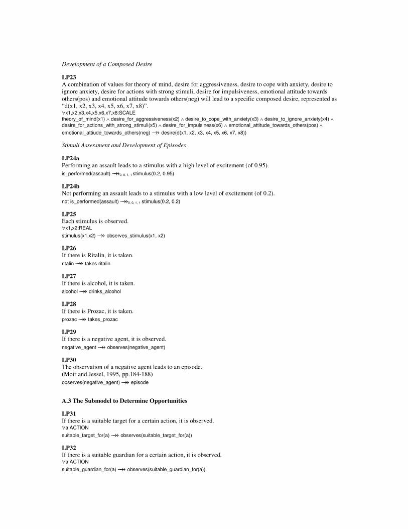
Development of a Composed Desire
LP23 A combination of values for theory of mind, desire for aggressiveness, desire to cope with anxiety, desire to
ignore anxiety, desire for actions with strong stimuli, desire for impulsiveness, emotional attitude towards
others(pos) and emotional attitude towards others(neg) will lead to a specific composed desire, represented as
“d(x1, x2, x3, x4, x5, x6, x7, x8)”. ∀x1,x2,x3,x4,x5,x6,x7,x8:SCALE theory_of_mind(x1) ∧ desire_for_aggressiveness(x2) ∧ desire_to_cope_with_anxiety(x3) ∧ desire_to_ignore_anxiety(x4) ∧
desire_for_actions_with_strong_stimuli(x5) ∧ desire_for_impulsiness(x6) ∧ emotional_attitude_towards_others(pos) ∧
emotional_attiude_towards_others(neg) →→ desire(d(x1, x2, x3, x4, x5, x6, x7, x8))
Stimuli Assessment and Development of Episodes
LP24a
Performing an assault leads to a stimulus with a high level of excitement (of 0.95).
is_performed(assault) →→0, 0, 1, 1 stimulus(0.2, 0.95)
LP24b Not performing an assault leads to a stimulus with a low level of excitement (of 0.2).
not is_performed(assault) →→0, 0, 1, 1 stimulus(0.2, 0.2)
LP25 Each stimulus is observed. ∀x1,x2:REAL stimulus(x1,x2) →→ observes_stimulus(x1, x2)
LP26 If there is Ritalin, it is taken.
ritalin →→ takes ritalin
LP27 If there is alcohol, it is taken.
alcohol →→ drinks_alcohol
LP28 If there is Prozac, it is taken.
prozac →→ takes_prozac
LP29 If there is a negative agent, it is observed.
negative_agent →→ observes(negative_agent)
LP30 The observation of a negative agent leads to an episode.
(Moir and Jessel, 1995, pp.184-188)
observes(negative_agent) →→ episode
A.3 The Submodel to Determine Opportunities
LP31 If there is a suitable target for a certain action, it is observed. ∀a:ACTION
suitable_target_for(a) →→ observes(suitable_target_for(a))
LP32 If there is a suitable guardian for a certain action, it is observed. ∀a:ACTION
suitable_guardian_for(a) →→ observes(suitable_guardian_for(a))
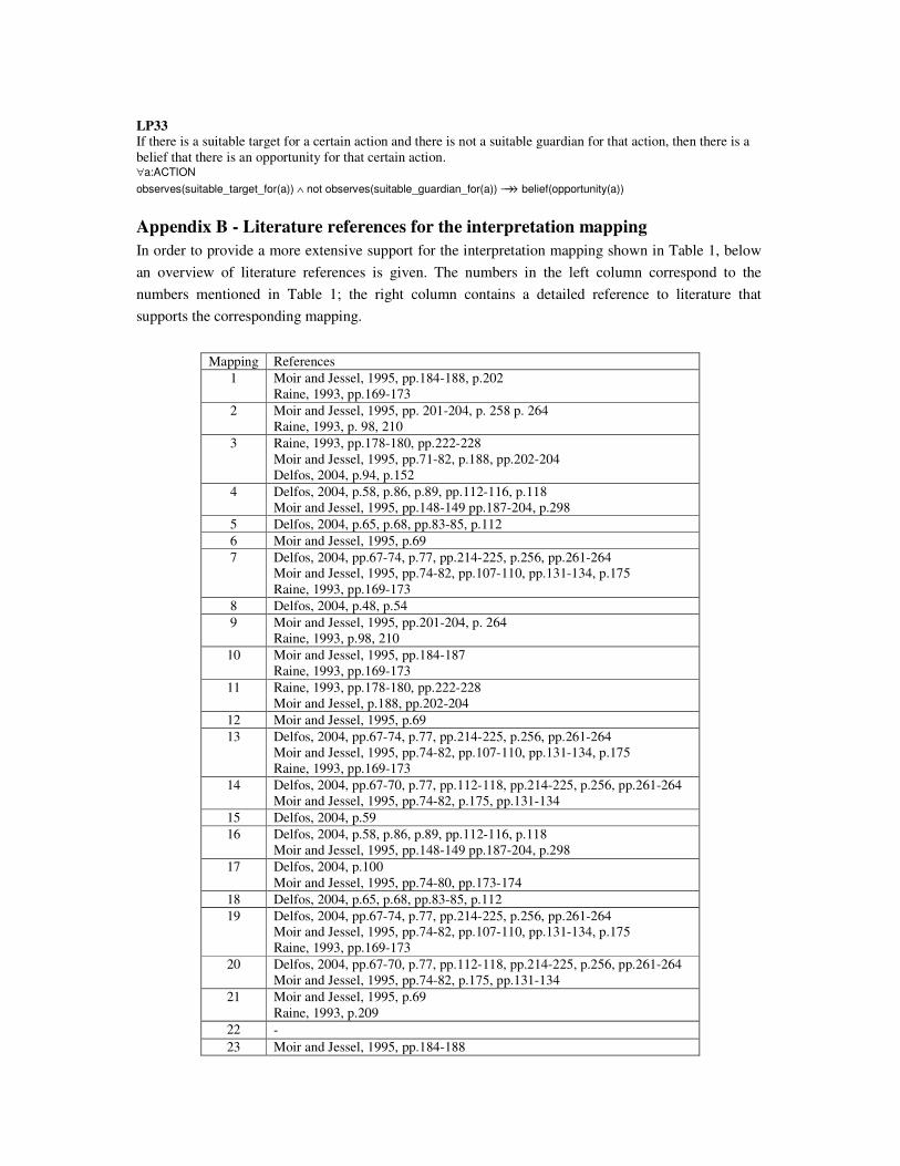
LP33 If there is a suitable target for a certain action and there is not a suitable guardian for that action, then there is a
belief that there is an opportunity for that certain action. ∀a:ACTION
observes(suitable_target_for(a)) ∧ not observes(suitable_guardian_for(a)) →→ belief(opportunity(a))
Appendix B - Literature references for the interpretation mapping
In order to provide a more extensive support for the interpretation mapping shown in Table 1, below
an overview of literature references is given. The numbers in the left column correspond to the
numbers mentioned in Table 1; the right column contains a detailed reference to literature that
supports the corresponding mapping.
Mapping References
1 Moir and Jessel, 1995, pp.184-188, p.202
Raine, 1993, pp.169-173
2 Moir and Jessel, 1995, pp. 201-204, p. 258 p. 264
Raine, 1993, p. 98, 210
3 Raine, 1993, pp.178-180, pp.222-228
Moir and Jessel, 1995, pp.71-82, p.188, pp.202-204
Delfos, 2004, p.94, p.152
4 Delfos, 2004, p.58, p.86, p.89, pp.112-116, p.118
Moir and Jessel, 1995, pp.148-149 pp.187-204, p.298
5 Delfos, 2004, p.65, p.68, pp.83-85, p.112
6 Moir and Jessel, 1995, p.69
7 Delfos, 2004, pp.67-74, p.77, pp.214-225, p.256, pp.261-264
Moir and Jessel, 1995, pp.74-82, pp.107-110, pp.131-134, p.175
Raine, 1993, pp.169-173
8 Delfos, 2004, p.48, p.54
9 Moir and Jessel, 1995, pp.201-204, p. 264
Raine, 1993, p.98, 210
10 Moir and Jessel, 1995, pp.184-187
Raine, 1993, pp.169-173
11 Raine, 1993, pp.178-180, pp.222-228
Moir and Jessel, p.188, pp.202-204
12 Moir and Jessel, 1995, p.69
13 Delfos, 2004, pp.67-74, p.77, pp.214-225, p.256, pp.261-264
Moir and Jessel, 1995, pp.74-82, pp.107-110, pp.131-134, p.175
Raine, 1993, pp.169-173
14 Delfos, 2004, pp.67-70, p.77, pp.112-118, pp.214-225, p.256, pp.261-264
Moir and Jessel, 1995, pp.74-82, p.175, pp.131-134
15 Delfos, 2004, p.59
16 Delfos, 2004, p.58, p.86, p.89, pp.112-116, p.118
Moir and Jessel, 1995, pp.148-149 pp.187-204, p.298
17 Delfos, 2004, p.100
Moir and Jessel, 1995, pp.74-80, pp.173-174
18 Delfos, 2004, p.65, p.68, pp.83-85, p.112
19 Delfos, 2004, pp.67-74, p.77, pp.214-225, p.256, pp.261-264
Moir and Jessel, 1995, pp.74-82, pp.107-110, pp.131-134, p.175
Raine, 1993, pp.169-173
20 Delfos, 2004, pp.67-70, p.77, pp.112-118, pp.214-225, p.256, pp.261-264
Moir and Jessel, 1995, pp.74-82, p.175, pp.131-134
21 Moir and Jessel, 1995, p.69
Raine, 1993, p.209
22 -
23 Moir and Jessel, 1995, pp.184-188
Copyright © 2022 FDOKUMEN

