Pergamon Adv. Space Res. Vol. 23, No. 11, pp. 1801-1807.1999

0 1999 COSPAR. Published by Elsevier Science Ltd. All rights reserved Printed in Great Britain

www.elsevier.nl/locate/asr PII: SO273-1177(99)00534-7 0273-l 177199 $20.00 + 0.00

OF LUNAR GRAVITY FIELD SOLUTIONS ON THE INF RMATION CONTENTS AND REGULARISATION

Rune Floberghagen, Johannes Bouman, Radboud Koop and Pieter Visser

Delft Institute for Earth-Oriented Space Research (DEOS), Kluyverweg 1,2629 HS, Delft, The Netherlands, phone: + 31 15 2786221, fax: + 31 15 278 5322, email: Rune.Floberghagen@lr.tudelft.nl

ABSTRACT

Till the present day the recovery of the lunar gravity field from satellite tracking data depends in a crucial way on the level and method of regularisation. With Earth-based tracking only, the spatial data coverage is limited to only slightly more than 50% and the inverse problem remains severely ill-posed. The development of global gravity models suitable for precise orbit modeling as well as geophysical studies therefore requires a significant level of regularisation, limiting the solution power over the far-side where no gravity information is available. Unconstrained solutions, within the framework of global harmonic base functions, are only possible for very low degrees (< 10). Any significant change to this situation is only to be expected when global satellite-to-satellite tracking data of high quality becomes available early in the next decade. Yet, a rigorous analysis of the impact of the chosen method and level of regularisation is lacking. Most gravity models employ a Kaula-type signal smoothness constraint of 15 x 10m5/Z2, which allows a good overall data fit as well as a smooth field over the far-side. Furthermore, a geographical type of constraint has been suggested, where surface accelerations have been introduced in areas of no data coverage. Modem numerical methods, on the other hand, offer direct tools and search mechanisms for the optimal level of regularisation. This paper presents a study of Tikhonov-type regularisation of lunar gravity solutions, with emphasis on the so-called L- curve and quasi-optima& methods for regularisation parameter estimation. Furthermore, new quality measures of lunar gravity solutions are presented, which account for the bias introduced by the regularisation.

INTRODUCTION 0 1999 COSPAR. Published by Elsevier Science Ltd.

The gravitational potential V of any near-spherical body is usually expressed in terms of spherical harmonics

where 1, m are the degree and order, GM the lunar gravity parameter, R some reference radius, r, 4, X the selenocen- tric polar coordinates (radius, latitude, longitude), l$, the spherical harmonic basis functions and Kl,,, E {cl,, &,} the fully normalized coefficients to be determined (Heiskanen and Moritz, 1967). The recovery of V from satellite tracking data is an ill-posed inverse problem. First, satellites orbit at a certain altitude above the lunar surface which dampens the high-frequency information. Secondly, the data coverage is (till date) inhomogeneous in space and in time. In addition, every measurement type has its limitations and will, in the frequency domain, exhibit a different sensitivity for different orbital frequencies. Finally, systematic modeling errors may occur, e.g. absent or incomplete models of radiation pressure effects.

As a consequence, the determination of the gravitational potential from satellite tracking data is typically unstable and regularisation is required. In space geodesy and selenodesy this is typically handled by adding a diagonal weight matrix (inverse a priori variance-covariance matrix) to the least-squares normal matrix system, where the weights are usually taken from Kaula’s rule-of-thumb (Kaula, 1966). A further refinement of this rule may be applied by estimating a scaling factor which seeks to compromise between data fit and the overall smoothness of the least- squares solution. For example, till the present day the signal constraint as applied to gravity coefficients &, and sll,

1801

1802 R. Floberghagen et al.

in the case of the Moon is given by

{Cl,, 31,) - 0 f fl xl;o-5 where /3 is the empirically determined constant. For GLGM-2 (Lemoine et al., 1997) and Lun60d (Konopliv et al., 1993) /I = 15, whereas Kaula (1963) in his original work suggested a value of 35. The a priori variance-covariance matrix added to the normal equation system is then the diagonal matrix with elements given by cr x 101014, where Q = l/p2. By the application of such constraints the solution is biased towards zero while its variance will approach the constraint value. A variant is suggested by Konopliv et al. (1994), where surface accelerations are added in areas where no direct measurements are available. The Kaula rule is used to predict the accelerations and a fixed measurement variance is applied in the weight matrix. This ‘geographical’ constraint is, hence, a more indirect Kaula constraint.

The selenophysical interpretation of Kaula’s rule is that it predicts the power of the gravity field, and as such it is used as a smoothness constraint during inversion. However, the constant in Kaula’s rule is determined by trial and error and cannot be adequately determined without knowing the actual gravity field. A study of recent literature on numerical methods for inverse problems, however, reveals a number of more sophisticated methods for determination of the optimal Q for regularisation purposes. The scope of this paper is the description and application of two such new methods, namely the L-curve method and the quasi-opfimulity criterion. Due to the bias introduced in the solution, the collocation framework for the quality description of the solution, which is unbiased by definition, is no longer valid. The mean square error matrix, which is the sum of the propagated variance-covariance matrix and the squared bias (another word is regularisation error) is therefore introduced as a more realistic quality measure.

The two problems outlined above, the determination of the optimal level or regularisation and the alternative ways to describe the solution quality, are investigated on the basis of the normal equation system of the GLGM-2 model (Lemoine et al., 1997). Since it is beyond the scope of this paper to derive a completely new lunar gravity model, actual tracking data is not processed. Instead, a linear model relating the observations and the unknowns is assumed, based on the GLGM-2 normal equation system. Next, the quality analysis of lunar gravity models is presented, using GLGM-2 as an example. Finally, the L-curve and quasi-optimality methods for regularisation parameter estimation are presented. Results as found for the GLGM-2 normal matrix are presented and compared to the Kaula-rule applied in GLGM-2.

THE LINEAR MODEL AND ITS SOLUTION

In general the relationship between the observations ye = y + e, with y the exact observation and e the data noise, and the unknowns z is non-linear, i.e. E{ye} = E(y) = A(z), where A is the functional relating the observations to the unknowns. E{} is the expectation operator and it is assumed that E(e) = 0 and E{eeT} = a21, i.e. model errors are not considered in the present analysis. Inverting for the selenopotential is done by linearising the relationship between observations and unknowns and solving for corrections to the a priori model in an iterative fashion. Hence, in practical cases one has

ye=y+e=Az+e (2)

where E{ye} = E(y) = A z, where A is now the design matrix. The vector of unknowns of course contains the gravity field coefficients {cl,, ,!$,}. The least-squares solution 21, is the best linear unbiased estimate of the solution. Taking account of a possible weighting of different data sets in the solution, represented by the weight matrix (inverse error covariance of the measurements) P, the familiar least-squares solution reads

xls = (KPA)-l ATpye

If the problem at hand is perfectly observable, xl8 may be considered a stable solution to our inverse problem. How- ever, the complications of the measurements being inhomogeneously distributed in space and in time, as well as the damping of orbital perturbations with altitude causes xls to be unstable. That is, small data errors may cause large errors in the solution. In theory, this may be handled by either 1) limiting the number of unknowns to the ones with large singular values (i.e. those for which direct estimation is largely possible), or 2) applying regularisation to the

Lunar Gravjty Field 1803

normal equation system. While the first method may work for the estimation of small spherical harmonics expansions, it is known that the lunar potential is dominated by mass concentrations which are impossible to represent in terms of low-degree harmonics. Secondly, for gravity solutions with a resolution close to the satellite altitude, coefficients or groups of coefficients (lumped coefficients) will remain below the data noise level and it might still not be possible to compute a stable ( ATP~) -‘. This is further illustrated by computing the singular value decomposition of the design matrix A = VCF, where U and V are orthonormal matrices spanning the space of the observations and the mea- surements, respectively, and C is a diagonal matrix with elements {oi]ol > ~72 2 . . . 2 (T, > 0} and limi,, ui = 0. Let P = I (not essential in this context), then

21s = (VCUTUCVT)-lVCUTye

= (VC2vT)-*VCUTye = VC-‘UTy”

= VCwlUT(y + e) = 2 + VC-‘UTe (4)

Thus, the least-squares solution consists of the exact solution x from ‘exact’ observations y and a term which depends on the noise e. Because the elements of C tend to zero, due to the essentially one-hemisphere data coverage and the satellite altitude, the noise is amplified with a large number and instability occurs.

A priori information on the coefficient power as given by Kaula may be used to increase stability. With the elements of the diagonal Kaula matrix K given by lOlo x L4, the regularised least-squares solution becomes

2, = (A=PA + d)-l A=P~~

Eq. 5 is equivalent to the least-squares collocation solution (Marsh et al., 1988). However, due to the constraint, it is also biased towards zero, which is impossible for a collocation solution. Error assessment based on the collocation framework is therefore considered impossible, and, hence, it is more appropriate to consider Eq. 5 as a biased estimator. The expectation of Eq. 5 is

E{x,} = (ATPA + c&)-~A=PE{~“> = (ATPA + c&)-~A=PAx

# 2,

and the bias introduced by the constraints is

E{z, - x} = 6x = -(ATPA + cxK)%Kx (6)

The bias may become larger than the coefficient value. One difficulty with the bias is that the true solution x is involved. Obviously, these coefficients are unknown and estimating the bias with biased coefficients will give too op- timistic results since the power of these coefficients is too low. This is another reason why a pure variance-covariance propagation may lead to optimistic estimates of the true solution quality. For GLGM-2, which forms the test case of the present analysis, the coefficient biases are larger than 50% of the coefficient value for nearly all harmonics beyond degree and order 30.

QUALITY ASSESSMENT

The mean square error matrix is introduced as a more realistic measure of the error in lunar gravity models. Since the solution is biased, it has two parts: the propagated error Q5 and the squared bias. Error propagation yields

QZ = (ATPA + cX)-‘ATPA(ATPA + aK)-’ (7)

The mean square error matrix MS. is therefore

MSEM = Qz + SsSxT

1804 R. Floberghagen er al.

Identical to the case of error variance-covaiiance matrices for unbiased estimators, the MSEM may be subject to error propagation, for example to selenoid height errors or to gravity anomaly errors, cf. Haagmans and Van Gelderen (1991).

One can also compute to which extent the observations contribute to the solution (and, vice versa, that of the a priori information). Bouman (1997) argues that a good measure for unbiased estimators is the change in the error covariance matrix of the estimation parameters due to the regularisation (which can be associated with the gain matrix in Kalman filtering):

contry = (ATPA + aK)-‘ATPA (9)

The diagonal elements of cmtr, E (0, 1). Zero means that the observations do not contribute to the determination of the unknown, ie. all information comes from the constraint, whereas a unit value implies that the observations completely determine that specific unknown. For biased estimators Bouman (1997) developed a similar measure:

contry = MSEM x MSEM-’ a=O (10)

contry shows a behaviour similar to that of the bias. Beyond degree and order eighteen less than 50% of the infor- mation comes from the tracking data, and from thirty onwards this is gradually reduced to less than lo%, which is basically seen as a proof of lack of information for global lunar gravity modelling.

DETERMINATION OF THE REGULARISATION PARAMETER FOR BIASED ESTIMATORS

‘B.vo methods for the determination of the optimal regularisation parameter cr under the presence of a bias are con- sidered, being the L-curve and the quasi-optimality criterion, cf. Hansen and O’Leary (1993) and Morozov (1984), respectively. The ideas of both methods are roughly the same. Consider the minimization of

44 = lb - YII; + 441~ which leads to Eq. 5. The norm on the left is the least-squares problem. Minimization of this term gives the smallest errors, but the norm of the solution is unconstrained. The second term controls the solution smoothness; however, this smoothness condition also causes the solution to become biased. The parameter (Y controls the compromise between smoothness of the solution, ie. I[z)(K remains small, and data fit, [IAs - yJI p small. Both the L-curve and the quasi- optimality criterion aim to find an cr such that other o’s close to it yield a comparable solution. In other words, the methods seek to balance the data error with the regularisation error.

L-curve

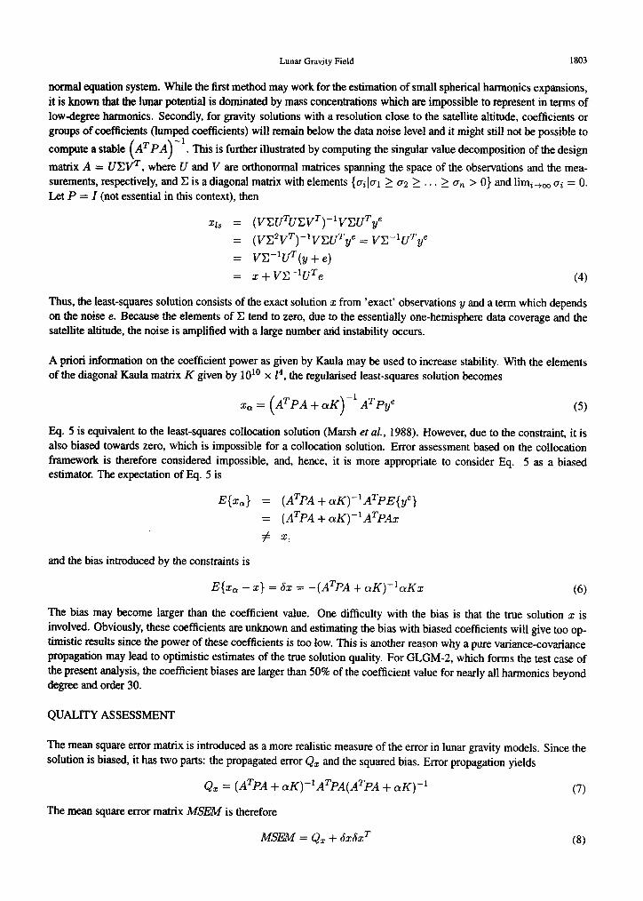
The L-curve is a plot, for all valid cr, of the norm lIza 11~ of the stable solution versus the corresponding residual norm IIAxa - yllp. It turns out that the L-curve, when plotted in log-log scale, has an L-shaped appearance. The vertical part of the curve corresponds to smaller ct. The emphasis of minimizing J(a) is on [[Ax, - yllp, allowing IIzCall~ to become large. The horizontal part of the L-curve corresponds to solutions where the residual norm (IAx, - yJlp is most sensitive to the scaling parameter because X~ is dominated by the bias, compare Hansen and O’Leary (1993); Hansen (1997). The comer of the L-curve is optimal in the sense that the change of both norms is equal for changing cr. This point may be located by maximum curvature. However, it may be shown that the minimum of the function

$4~) = 11~all~IIA~a - YIIP (11)

gives the same scaling parameter (Regmska, 1996). Note that Eq. 11 cannot be computed directly since the design matrix A is not available. This is generally the case in gravity field estimation from satellite tracking data where normal matrices for single arcs are combined to form a final normal equation system. However, the data errors behave like aZT1, compare Eq. 4, which can be determined by eigenvalue techniques. Hence, real observations ye may be approximated by Axe where xe = x + e. The obvious choice for the exact solution x is the GLGM-2 solution itself, the errors e arc assumed to be given by 3N(O, l)/ i ~7 x coefficient sigma, with N(0, 1) the standard normal

Lunar Gravity Field 1805

L-curve for GLGM-2

OE+O lE-3 2E‘a 3E-3 4E-8 SE-8

L-curve for GLGM-2 4 .95031)1~

I

-3.9580387

-3.9580388 t

-3.9580336 c ’ c c c ’ ’ 4 OE+O 2E-1 4E-1 BE-1 BE-1 lE+O 1ElO lE+O

II Ax - Y II

b

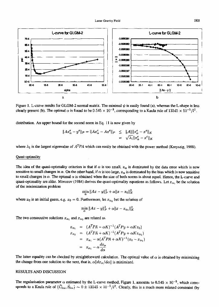
Figure 1. L-curve results for GLGM-2 normal matrix. The minimal 1c, is easily found (a), whereas the L-shape is less clearly present (b). The optimal (Y is found to be 0.545 x 10V8, corresponding to a Kaula rule of 13545 x 1W5/1’.

distribution. An upper bound for the second norm in Eq. 11 is now given by

IlAx: - yelb = IIAz: - AdIp L IMIIIG - ~~11~ = dm: - ZellK

where Xi is the largest eigenvalue of ATPA which can easily be obtained with the power method (Kreyszig, 1988).

Quasi-optimality

The idea of the quasi-optimality criterion is that if a is too small, 2, is dominated by the data error which is now sensitive to small changes in (Y. On the other hand, if cy is too large, Z, is dominated by the bias which is now sensitive to small changes in cr. The optimal (Y is obtained when the size of both norms is about equal. Hence, the L-curve and quasi-optimality are alike. Morozov (1984) derives the quasi-optimality equations as follows. Let z,, be the solution of the minimization problem

m$ IPa: - YII~ + 412 - ~011~

where ~0 is an initial guess, e.g. ~0 = 0. Furthermore, let z,, bet the solution of

m&lb - ~11; + 41~ - G, 11°K

The two consecutive solutions z,, and z,, are related as

X,1 = (ATPA + aK)-1 (ATPy + dx,,)

x02 = (ATPA + crK)-l(ATPy + c&x,,) = x,, - cr(ATPA + aK)-‘(x,, - x,,)

kk = XW -da: The latter equality can be checked by straightforward calculation. The optimal value of (Y is obtained by minimizing the change from one solution to the next, that is, ajldx,/dall is minimized.

RESULTS AND DISCUSSION

The regularisation parameter (Y estimated by the L-curve method, Figure 1, amounts to 0.545 x 10e8, which corre- sponds to a Kaula rule of {ct,, ,$,} N 0 f 13545 x 10P5/Z2. Clearly, this is a much more relaxed constraint (by

1806 R. Floberghagen et al.

- h8igMa fmm Optic npubffrd GLGM-2 klmold - from optimally rqubrhd GLGM-2 MSEN

a b

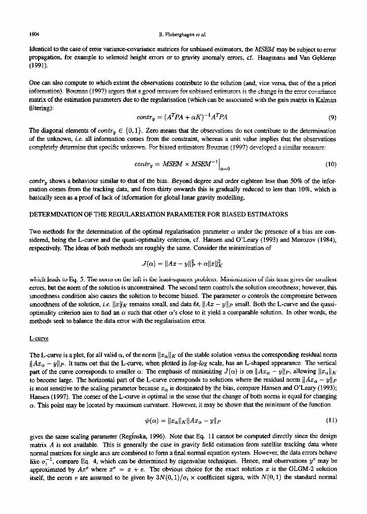
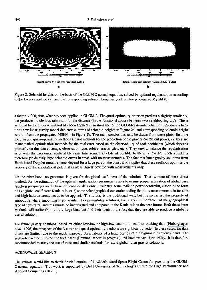
Figure 2. Selenoid heights on the basis of the GLGM-2 normal equation, solved by optimal regularisation according to the L-curve method (a), and the corresponding selenoid height errors from the propagated MSEM (b).

a factor N 900) than what has been applied in GLGM-2. The quasi-optimality criterion predicts a slightly smaller cx, but produces no obvious minimum for the distance (in the functional space) between two neighbouring za’s. The a as found by the L-curve method has been applied in an inversion of the GLGM-2 normal equation to produce a ficti- tious new lunar gravity model depicted in terms of selenoid heights in Figure 2a, and corresponding selenoid height errors - from the propagated MSEM - in Figure 2b. Two main conclusions may be drawn from these plots: first, the L-curve and quasi-optimality methods are not methods for the prediction of the gravity coefficient power, ie. they are mathematical optimisation methods for the total error based on the observability of each coefficient (which depends primarily on the data coverage, observation type, orbit characteristics, etc.). They seek to balance the regulatisation error with the data error, while at the same time remain as close as possible to the true inverse. Such a small LY therefore yields truly large selenoid errors in areas with no measurements. The fact that lunar gravity solutions from Earth-based Doppler measurements depend for a large part on the constraint, implies that these methods optimise the recovery of the gravitational potential in areas largely covered with measurements only.

On the other hand, no guarantee is given for the global usefulness of the solution. That is, none of these direct methods for the estimation of the optimal regularisation parameter is able to ensure proper estimation of global base function parameters on the basis of near-side data only. Evidently, some realistic power constraint, either in the form of 1) a global coefficient Kaula rule, or 2) some selenographical constraint adding fictitious measurements in far-side and high-latitude areas, needs to be applied. The former is the traditional way, but it also carries the property of smoothing where smoothing is not wanted. For present-day solutions, this argues in the favour of the geographical type of constraint, and this should be investigated and compared to the Kaula rule in the near future. Both these latter methods will suffer from a truly large bias, but find their merit in the fact that they are able to produce a globally useful solution.

For future gravity solutions, based on either low-low or high-low satellite-to-satellite tracking data (Floberghagen et al. 1996) the prospects of the L-curve and quasi-optimality methods are significantly better. In these cases, the data errors are limited, due to the much improved observability of a large portion of the harmonic frequency band. The methods have been tested for such cases (Bouman, report in progress) and have proven their ability. It is therefore recommended to study the use of these and similar methods for future global lunar gravity solutions.

ACKNOWLEDGEMENTS

The authors would like to thank Frank Lemoine of NASA/Goddard Space Flight Center for providing the GLGM- 2 normal equation. This work is supported by Delft University of Technology’s Centre for High Performance and Applied Computing (HPoC).

Lunar Gravity Field 1807

REFERENCES

Bouman, J., Quality assessment of geopotential models by means of redundancy decomposition?, DEOS Progress Letters., 97.1, pp. 49-54 (1997)

Floberghagen, R., R. Noomen, P.N.A.M. Visser and G.D. Racca, Global Lunar Gravity Recovery From Satellite-to- Satellite Tracking, Plant. Space Sci., 44(10), pp. 1081-1097 (1996)

Haagmans, R. and M. van Gelderen, Error variances-covariances of GEM-Tl: their characteristics and implications in geoid computation, J. Geophys. Rex, 96(B12), pp. 2001 l-20022 (1991)

Hansen, P, Regularization Tools, A MATLAB package for analysis and solution of discrete ill-posed problems, Dept. of Mathematical Modeling, Technical Univ. of Denmark, http://www.imm.dtu.d pch (1997)

Hansen, P., and D. O’Leary, The use of the L-curve in regularization of discrete ill-posed problems, SIAM .I. Sci. Comput., 14(6), pp. 1487-1503 (1993)

Heiskanen, W. and H. Moritz, Physical Geodesy, W.H. Freeman & Co. (1967) Kaula, W., The Investigation of the Gravitational Fields of the Moon and Planets With Artificial Satellites, Advun.

Space Sci. Technol., 5, pp. 210-230 (1963) Kaula, W., Theory of satellite geodesy, Blaisdell Pub. Co. (1966) Konopliv, A.S, W.L. Sjogren, R.N. Wimberly, R.A. Cook and A. Vijayaraghavan, A High Resolution Lunar Gravity

Field and Predicted Orbit Behavior, AAS paper 93-622 in Proc. of the AAS/AIAA Astrodynamics Specialist Con$, August 16-19, Victoria B.C., Canada (1993)

Konopliv, A.S. and W.L. Sjogren, Venus Spherical Harmonic Gravity Model to Degree and Order 60, ICARUS, 112, pp. 42-54 (1994)

Kreyszig, E., Advanced engineering mathematics, John Wiley & Sons, 6th edition (1988) Lemoine, F., M. Zuber, G. Neumann and D. Rowlands, A 70th degree lunar gravity model (GLGM-2) from Clementine

and other tracking data, J. Geophys. Res., 102(E7), pp. 16339-16359 (1997) Marsh, J., F. Lerch, B. Putney, D. Christdoulidis, D. Smith, T. Felsentreger, B. Sanchez, S. Klosko, E. Pavlis, T.

Martin, J. Williamson, 0. Colombo, D. Rowlands, W. Eddy, N. Chandler, K. Rachlin, G. Patel, S. Bhati and D. Chinn, A new gravitational model for the earth from satellite tracking data: GEM-Tl, J. Geophys. Res., 93(B6), pp. 6169-6215 (1988)

Morozov, V., Methods for solving incorrectly posed problems, Springer Verlag (1984) Regiriska, T., A regularization parameter in discrete ill-posed problems, SIAM J. Sci. Cornput., 17(3), pp. 740-749

(1996)