Final manuscript submitted to Journal of Physical Oceanography

On detection of a wave age dependency for the sea surface roughness

by

B. Lange Risø National Laboratory, Roskilde, Denmark

Present affiliation: University of Oldenburg, Oldenburg, Germany

H. K. Johnson DHI Water & Environment, Hørsholm, Denmark

S. Larsen

Risø National Laboratory, Roskilde, Denmark

J. Højstrup Risø National Laboratory, Roskilde, Denmark

H. Kofoed-Hansen

DHI Water & Environment, Hørsholm, Denmark

M. J. Yelland Southampton Oceanography Centre, Southampton, United Kingdom

Date received: ______________

Corresponding author address: Bernhard Lange Energy and Semiconductor Research Laboratory Department of Physics University of Oldenburg D-26111 Oldenburg Germany Phone: +49-441-798 3927 Fax: +49-441-798 3326 e-mail: Bernhard.Lange@uni-oldenburg.de

page 2 of 71

Abstract

The wave age dependency of the non-dimensional sea surface roughness (also called

the Charnock parameter) is investigated with data from the new field measurement

program at Rødsand in the Danish Baltic Sea. An increasing Charnock parameter with

inverse wave age is found, which can be described by a power law relation of the

form proposed by Johnson et al. (1998) and others.

Friction velocity is a common quantity in both the Charnock parameter and wave age.

Thus self-correlation effects are unavoidable in the relation between them. The

significance of self-correlation is investigated by employing an artificial 'data' set with

randomised wave parameters. It is found that self-correlation severely influences the

relation. For the Rødsand data set the difference between real and randomised 'data'

was found to be within the measurement uncertainty. By using a small sub-set of the

data it was found that the importance of self-correlation increases for a narrower

range of wave age values. This supports the conclusion of Johnson et al. (1998), that

due to the scatter and self-correlation problems the coefficients of the power law

relation can only be obtained from the analysis of an aggregated data set with a wide

wave age range combining measurements from several sites.

The dependency between wave age and sea roughness has been discussed extensively

in the literature with different and sometimes conflicting results. A wide range of

coefficients has been found for the power law relation between the Charnock

parameter and wave age for different data sets. It is shown that self-correlation

contributes to such differences, since it depends on the range of wave age values

present in the data sets. Also, data are often selected for rough flow conditions with

the Reynolds roughness number. It is shown that for data sets with large scatter this

page 3 of 71

can lead to misleading results of the relation of wave age and Charnock parameter.

Two different methods to overcome this problem are presented.

1 Introduction

The momentum transfer from the marine atmospheric boundary layer to the wind

driven water waves is important for all processes of air-sea interaction, such as wind

wave growth, storm surges and atmospheric circulation. It depends on the

aerodynamic sea surface roughness, which is therefore one of the most important

quantities for the description of the physical processes on both sides of the air-sea

interface.

Using dimensional arguments, Charnock (1955) suggested that the dimensionless sea

roughness gz0/u*2 (also called the Charnock parameter zch) is constant, where g is the

gravitational acceleration, z0 the sea surface roughness and u* the friction velocity.

Various field measurements showed that this is a reasonable concept for open ocean

sites, except for very low wind speeds (<3-4 m/s), although some increase of

Charnock parameter with wind speed has been found (see e.g. (Yelland and Taylor,

1996)). For sites near the coast the Charnock parameter has been found to vary from

site to site. Thus, zch is not a constant, but depends on other geophysical parameters.

It has been argued that these other parameters are properties of the wave field, i.e. that

the sea surface roughness is not only dependent on wind speed, but also on the wave

field present, which in turn is governed by wind, fetch and water depth. Different

attempts have been made to establish a relationship between the sea surface roughness

and different properties of the wave field like wave height, wave steepness or wave

age (e.g. Hsu, 1974, Donelan, 1990, Smith et al., 1992, Taylor and Yelland, 2001).

page 4 of 71

However, though it is general consensus that the sea surface roughness depends on the

wave field, the quantities suitable for description of this dependence are still a subject

of controversy.

Most authors have tried to improve the description of the sea surface roughness by a

parameterisation of the Charnock parameter with wave age (e.g. Smith et al. (1992),

Donelan et al. (1993), Johnson et al. (1998)). The latter group (hereafter called

JHVL98) showed that under specific conditions (discussed in section 2.5) the

Charnock parameter only depends on wave age. They describe this dependence with a

power law between the Charnock parameter (or normalised sea surface roughness),

zch, and the inverse wave age, u*/cp, in the form

%

S

FK ��

��

= * (1).

From an empirical fit to measurements from RASEX together with other previously

measured data sets they find the coefficients A=1.89 and B=1.59. One of the main

problems in these results was the conflicting, apparent trend of decreasing Charnock

parameter with inverse wave age in the RASEX data set taken alone (see also Taylor

and Yelland (2001)).

The problem with this kind of scaling is that the two quantities zch and wave age,

between which a functional relationship is proposed, are not independent of each

other. This can lead to self-correlation problems, i.e. the functional relationship might

be distorted or even determined by the common scaling variable. A theoretical

analysis of the self-correlation problem has been presented by Hicks (1978) and

specifically for the question of wave age dependent Charnock parameter by Smith et

al. (1992). The latter group concluded that self-correlation had an influence on the

results of the HEXOS data. JHVL98 generalised that this will always be the case for a

page 5 of 71

given site, where the fetch range is limited. They concluded that the combination of

data from several sites is necessary to minimise self-correlation. This conclusion is

also supported by a recent study by Drennan et al. (2003).

In the present paper we follow the JHVL98 approach with three principal aims:

1. To test the relation proposed by JHVL98 with a new, independent data set.

2. To investigate the influence of self-correlation on the relation.

3. To contribute to an understanding of the reasons for the conflicting results found by

JHVL98 and in the literature (see e.g. Toba et al. (1990), Drennan et al. (2003), Maat

et al. (1991)) by investigating how self-correlation and the data analysis method could

influence the resulting trend.

The plan of the paper is as follows: In section 2 the Rødsand field measurement

program is presented and the preparation of the measured data described. In section 3

these data are analysed in different ways. The results are compared with each other

and with published results. The influence of self-correlation on the relation is

investigated in section 4. The data analysis method is discussed in section 5 to gain a

better understanding of the relationship between Charnock parameter and wave age.

In the final section 6 the conclusions of the paper are summarised.

2 The Rødsand field measurement program

2.1 Site

A 50 m high meteorological measurement mast was established at Rødsand in

October 1996 as part of a Danish study of wind conditions for proposed offshore wind

page 6 of 71

farms. Simultaneous wind and wave measurements were performed from April 1998.

The mast is situated about 11 km south of the island Lolland in Denmark

(11.74596°E, 54.54075°N). The location of the mast is shown in Figure 1. The mast is

located in 7.7 m mean water depth with an upstream fetch of 30 to 100 km (and

above) from the SE to WNW sector (120°N to 290°N). The water depth slowly

increases to an average upstream depth of about 20 to 25 m in this sector. In the NW

to N sector (300°N to 350°N), the water depth is relatively shallower (from 1 m to 7

m) and the fetch is smaller (about 10 km to 20 km).

2.2 Instrumentation and Measurements

The instrumentation of the measurement mast is listed in Table 1. Wave and current

data are collected simultaneously with several atmospheric parameters. About 5900

half-hourly records with simultaneous wind and wave measurements have been

recorded. A more detailed description of the instrumentation and data can be found in

Lange et al. (2001).

Cup anemometers

Mean wind speeds and variances are derived from cup anemometers located at three

heights (see Table 1). Calibrated instruments of the type Risø P2546a are used. The

calibration accuracy is estimated to be +/- 1%. Data are corrected for flow distortion

errors due to the structure on which the anemometer is mounted, i.e. the mast and the

booms (see section 2.4.2). However, a correction uncertainty remains, and the overall

uncertainty of the wind speed measurement with cup anemometers is estimated to be

+/- 3%.

Wind vane

page 7 of 71

A wind vane of the type Risø Aa 3590 is used. The uncertainty of the instrument itself

is negligible. However, the adjustment of the orientation of the instrument is difficult

in the field and the absolute accuracy is estimated to be about +/-5º.

Sonic anemometer

The sonic anemometer is of the type Gill F2360a and is mounted at 46.6 m height

(42.3m from 12/May/99) above MSL (mean sea level). It measures wind speed in

three components (x,y,z) and air temperature with a resolution of 20 Hz. Fluxes are

calculated after turning the co-ordinate system such that the mean bias in the vertical

and crosswind components are zero. Remaining biases were found to be very small

(below 1 cm/s) and neglected.

Errors due to flow distortion of the measuring mast have been corrected for (see

section 2.4.2), although remaining errors have to be expected especially for friction

velocity measurements. Additionally, sonic anemometers experience an array flow

distortion, since transducers and struts of the instrument distort the wind flow in the

measurement volume. For the horizontal wind speed component flow distortions are

corrected with an individual calibration curve supplied by the manufacturer. This is

not the case for the vertical wind component. Mortensen and Højstrup (1995) report

systematic differences in a field experiment of typically 5% in mean wind speed and

10-15% in friction velocity between different sonic anemometer types. From wind

tunnel measurements they find that the errors are dependent on temperature and mean

wind direction. However, they state that further investigations are necessary before a

correction method can be established. Therefore no attempt has been made to correct

the measurements of the sonic anemometer for array flow distortion. The estimated

accuracy for the horizontal wind speed component is about +/- 5%. For the friction

page 8 of 71

velocity derived by eddy-correlation it is +/- 10%. Both errors are expected to contain

a wind direction dependent bias.

Additionally statistical errors due to sampling variability have to be considered, which

are responsible for the scatter in the data. Using the approximation of Wyngaard

(1973) derived from the Kansas data, the expected accuracy for the u* measurements

is about 10% for an eddy-correlation measurement at 45 m height with an averaging

time of 30 minutes and a mean wind speed of 10 m/s. It is mainly this sampling

variability which is responsible for the unavoidable scatter in the u* data.

Acoustic wave recorder

Waves are measured by an acoustic wave recorder (AWR), which is a SONAR-type

instrument positioned under water on a support structure. The type is the HD-

AWR201 from DHI Water & Environment.

The instrument is located about 100 m south-west of the offshore meteorological mast

at Rødsand since March 1998. The instrument was placed 3.74 m above the sea

bottom; the average water level during the measurement was 7.7 m. The instrument

measures the distance from the acoustic transducer to the water surface with a

sampling rate of 8 Hz.

The cut-off frequency of the instrument is determined by its spatial resolution (area

sampled by the acoustic transducer at the surface) rather than its sampling rate. It is

estimated to be about 0.8 Hz. The measured time series of water level fluctuations

was passed through a simple filter in order to remove local spikes in the data. A fixed

speed of sound (1475 m/s) is used independent of actual water temperature and

salinity. Water temperature and salinity ranges have been estimated for the site. They

lead to a maximum measurement error of -4% to +1% in the water level value and

wave height.

page 9 of 71

Water current measurement

The water current sensor is a two dimensional electromagnetic sensor measuring the

water velocity in x- and y-direction, manufactured by GMI (Geophysical and Marine

Instrumentation, Denmark). It is located 5.3 m above the sea bottom. The

measurement accuracy of the sensor is estimated to be +/- 2%.

2.3 Derived measured quantities

2.3.1 Friction velocity

Co-variances are calculated from the sonic anemometer measurements. Linear trends

remaining in the time series after selection for stationary conditions (see section 2.5)

are removed before calculation of the co-variances. Friction velocity is calculated

with the eddy-correlation method as:

( ) 25.022’’’’ ����� +=∗ (2)

The uncertainty in the friction velocity measurement is estimated to be about +/- 10%

as a combination of the general measurement uncertainty of the instrument and a

direction dependent error due to flow distortion.

If the direction dependent error coincides with a wind direction dependent distribution

of wave ages in the data, this error can distort the trend of sea surface roughness with

wave age. This is investigated by comparing the observed trend with the one found in

an analysis without using the sonic anemometer, where the friction velocity is derived

from the wind speed variance measurement of a cup anemometer.

For near neutral atmospheric stability, friction velocity u* and standard deviation of

the wind speed σu are proportional:

page 10 of 71

�� X

σ=∗ (3)

The constant C is estimated for the Rødsand data set by comparing the standard

deviation measured with the cup anemometer at 50 m height and the friction velocity

derived from the sonic anemometer at 46.6 m (42.3 m) height. The ratio of both is

plotted versus the stability parameter 50/L in Figure 2. No dependence on

atmospheric stability can be found for the near neutral stability range used. A possible

dependence of C on wave age, which could distort the trend of Charnock parameter

versus wave age, is investigated in Figure 3. Also here no significant dependence can

be found. The mean value for C is 2.42 with a standard deviation of 0.51, which is

about 20%. This is in the range of commonly used values: Garratt (1992) quotes 2.4

for flat terrain, Stull (1988) lists values from 2.47 to 2.57.

The measured value for C is used to derive friction velocities from the three cup

anemometer measurements. They provide complementary indirect measurements of

the friction velocity, which are expected to have no wind direction dependent error.

2.3.2 Neutral wind speed at 10 m height

The measured mean wind speed has been corrected for influences of the atmospheric

stability, described by the Monin-Obukov-length L. This L has been determined from

the measurements of the friction velocity, u*, the heat flux, <w'Θ'>, and the potential

temperature at 10 m, Θ:

Θ′′Θ

−=�

��

κ

3* (4)

The von Karman constant κ is taken as 0.4 and the gravitational constant g as 9.81

m/s2. The error in L due to humidity can be neglected since the humidity influence is

page 11 of 71

to a large degree included in the heat flux measurement of the sonic anemometer,

which measures the sound virtual temperature (see e.g. Schotanus, 1983). The

stability function Ψ is calculated by the standard approach (see e.g. Geernaert et al.,

(1986), JHVL98) and the neutral wind speed Q

�10 is derived from the measured wind

speed ���by:

Ψ+=

���

Q

10*1010 κ

(5)

Deviations of the measurement height from 10 m due to water level variations have

been accounted for by a log-linear wind profile with Charnock sea surface roughness

(with zch=0.018) and the measured stability parameter.

2.3.3 Sea surface roughness

For the calculation of sea surface roughness the measurements of friction velocity u*,

either from sonic or cup anemometer measurements (see section 2.3.1), and of the

neutral wind speed at 10 m height Q

�10 have been used. The friction velocity has been

corrected to its surface value (see section 2.4.1). The roughness length is calculated

from the logarithmic wind profile:

=

*

0)(

exp���

��

Qκ

(6)

The dimensionless sea surface roughness or Charnock parameter is defined as:

==

*

2*

2*

0

)(exp

���

�

��

�

���

Q

FK κ (7)

page 12 of 71

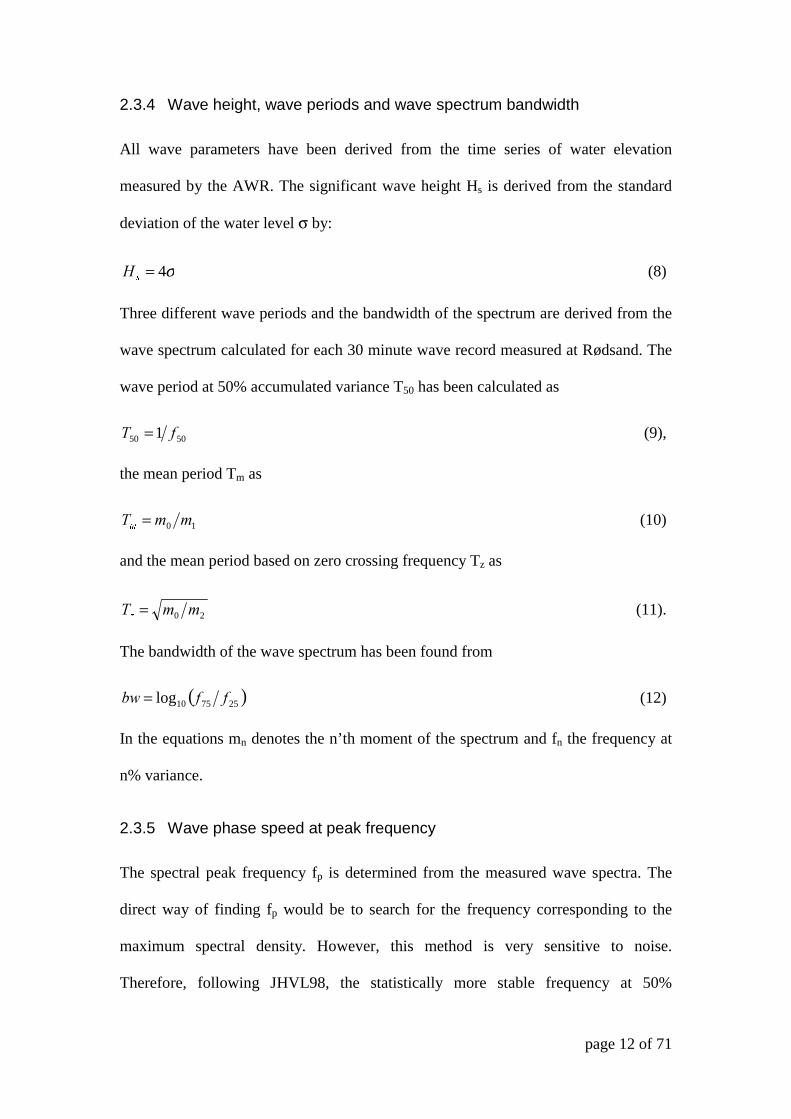
2.3.4 Wave height, wave periods and wave spectrum bandwidth

All wave parameters have been derived from the time series of water elevation

measured by the AWR. The significant wave height Hs is derived from the standard

deviation of the water level σ by:

σ4=V

� (8)

Three different wave periods and the bandwidth of the spectrum are derived from the

wave spectrum calculated for each 30 minute wave record measured at Rødsand. The

wave period at 50% accumulated variance T50 has been calculated as

5050 1 � = (9),

the mean period Tm as

10 �� P

= (10)

and the mean period based on zero crossing frequency Tz as

20 �� ]

= (11).

The bandwidth of the wave spectrum has been found from

( )257510log ���� = (12)

In the equations mn denotes the n’th moment of the spectrum and fn the frequency at

n% variance.

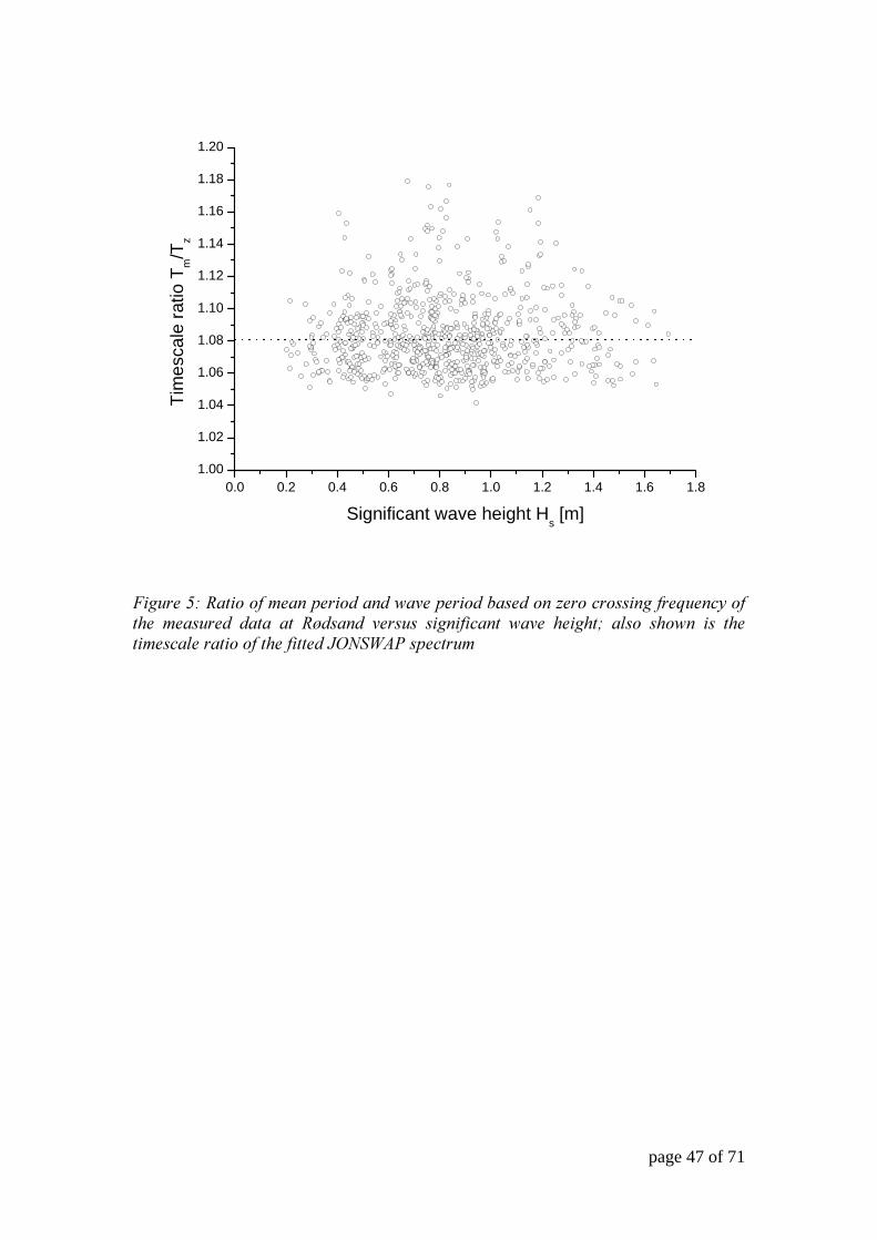
2.3.5 Wave phase speed at peak frequency

The spectral peak frequency fp is determined from the measured wave spectra. The

direct way of finding fp would be to search for the frequency corresponding to the

maximum spectral density. However, this method is very sensitive to noise.

Therefore, following JHVL98, the statistically more stable frequency at 50%

page 13 of 71

accumulated variance f50 is determined first and the measured f50 is then converted to

fp by using a mean wave spectrum shape.

The JONSWAP spectral model (Hasselmann et al., 1973) is used as shape function to

find the average ratio f50/fp, which best fits the measured spectra. The average values

of the parameters for the fitted spectrum are γ=1.58 (the peakedness parameter),

f50/fp=1.11, bw=0.153 and Tm/Tz=1.081. These compare well with the measured

bandwidth and timescale ratio as shown in Figure 4 and Figure 5, respectively.

The phase speed at peak frequency cp is calculated using the measured water depth

and spectral peak frequency fp in the linear dispersion relation.

2.4 Data corrections

2.4.1 Correction of the wind stress measurement for elevation

To a first approximation it is usually assumed that the flux in the surface layer is

independent of height, implying that the friction velocity is constant. However, this

assumption is not entirely correct and for near-neutral and stable conditions the

friction velocity decreases slightly with height. Since the determination of the sea

surface roughness is very sensitive to the value of the friction velocity, this deviation

is accounted for in the determination of the surface friction velocity.

Donelan (1990) derives the following expression from an analysis of the horizontal

momentum equation at the surface and the top of the boundary layer, when no

observed boundary-layer height is available:

)1()(*,

02*,*

V

F

V ���

���α−= (13)

page 14 of 71

where )(* �� is the friction velocity measured at height z, V

�*, is the friction velocity at

the surface,V

J

�

�

*,0 =α is the ratio of geostrophic wind vg and

V�*, (taken as 120 =α ), fc

the Coriolis parameter (1.46 10-4 sin(φ), with φ latitude).

A direct comparison of this equation with measured friction velocities can not be

made with the Rødsand data set, since a sonic anemometer is only available at one

height. However, friction velocities derived from cup anemometer measurements of

wind speed variances at the three heights 10 m, 30 m and 50 m can be compared. The

difference between friction velocities derived from cup anemometer variances at 10 m

and 50 m height versus stability parameter is shown in Figure 6, the difference

between 10 m and 30 m is shown in Figure 7. A height dependence of the friction

velocity is observed, which is independent of stability for the near-neutral stability

range used. The mean difference over the height difference of 40.1 m is 0.036 m/s

(i.e. 0.0009 m/s per meter), over the height difference of 19.6 m it is 0.021 m/s

(0.0011 m/s per meter). The mean decrease of friction velocity with height of 0.00071

m/s per meter height difference from equation (13) is consistent with the data for both

height differences. The average measured value has been used to derive the friction

velocity at the surface from friction velocities derived at different heights from sonic

and cup anemometer measurements.

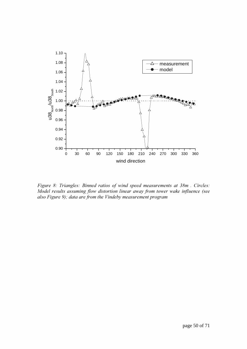
2.4.2 Correction of wind speeds for flow distortion of the measurement mast

At the Rødsand measurement mast, all cup anemometers as well as the sonic

anemometer are mounted on booms pointing in the same direction of about 265°.

Flow distortion from the measurement mast and the mounting of the instruments leads

page 15 of 71

to measurement errors. They are obviously very large for situations with direct mast

shade and such records (wind directions 85° +/- 35°) were omitted.

For other wind directions, a linear correction model was used, which was developed

by Højstrup (1999) from measurements at a similar mast at the Vindeby site. In order

to investigate the effects of flow distortion from the tower at the Vindeby site,

anemometers were mounted at opposite sides of the mast at three different levels for a

period of seven months. A triangular lattice measurement mast was used with a tower

side length of 1.21 m and a boom length (measured from the nearest corner of the

tower) of 2.51 m at 7 m height, leading to a boom length to tower side ratio of about

2. At 20 m and 38 m height it was about 2.5 and 4, respectively, with a tower side

length of 0.95 m and 0.60 m and a boom length of 2.40 m and 2.32 m, respectively.

The boom directions were 50º and 230º.

Taking the ratio of wind speeds on opposite sides of the tower, averaging in direction

bins, a similar picture for all three heights (see Figure 8 where only the highest height

is shown) can be seen. Also in Figure 8 the result of a simple model (Højstrup, 1999)

is shown, assuming that the tower induced flow distortion is linear in wind direction,

away from the sectors directly influenced by the wake of the tower. From Figure 8 it

is noted that the simple linear model works well outside of the sectors where one of

the anemometers is in the wake of the mast and the other anemometer. For the three

heights at Rødsand, correction factors of 1.033/0.994 (maximum increase and

decrease), 1.012/0.998 and 1.004/0.999 for the three heights 10 m, 30 m and 50 m,

respectively, are used for all wind speeds. The factors for 50 m height are also used

for the sonic anemometer mean wind speed and friction velocity. These are illustrated

in Figure 9 for all three heights.

page 16 of 71

Flow distortion of the wind speed standard deviation and the friction velocity is

assumed to be similar to that of the mean wind speed and the same correction factors

are used for a simple correction. This approach is compared with measurements at

Vindeby in Figure 10. Ratios of wind speed standard deviations of the two

anemometers are shown, similar to Figure 8. A reasonable agreement between model

and measurement is found.

2.4.3 Transformation of wind speeds to water following co-ordinates

For the interaction of wind with waves the relevant wind speed is the difference

between air and water movement. Wind measurements made from fixed structures,

like the measurement mast at Rødsand, therefore need to be corrected for the water

current. At Rødsand, the water current is measured at a mean water depth of 2.4 m.

Differences between the current at this depth and the surface current have been

neglected and all mean wind speeds measured at the mast have been transformed to

refer to the moving reference frame of the water surface.

At Rødsand currents are generally slow, usually below 0.4 m/s, and only in some

occasions reach values of up to 0.65m/s. Differences in wind speed due to the

transformation are for 93% of the records below 2% and for 99% below 5%.

2.5 Data selection

The first step in data selection is the rejection of data from nonstationary situations,

i.e. where the ambient conditions change too much during the 30 minutes of the

record under investigation. For the most important quantities the change in time is

computed for a time period of 30 minutes before to 30 minutes after the averaging

period of the record. Time periods with large gradients are rejected. This was done for

page 17 of 71

wave phase speed, 10 m wind speed, friction velocity and wind direction. Gradients of

not more than 20% per hour were allowed for wave phase speed and wind speed, 30%

for friction velocity and 40º for wind direction. Due to this selection, 83% of all

measured records were rejected.

The second step is to reject measurements where the derived measured quantities can

not be calculated. This is the case if the measurement height of the sonic anemometer

of about 45 m is above the surface layer. This can lead to friction velocity

measurements which can not be transformed to the surface value. As a simple

approximation, the height of the surface layer can be estimated as 10% of the

boundary layer height zh, which is estimated by Tennekes (1982) as:

F

V

K ��

� .*25.0= ( 14)

Using this expression it is found that the surface layer might be shallower than 45 m if

u* is smaller than about 0.2 m/s. Such measurements have been rejected.

The third step is to select only measurements where the conditions required by the

theory under investigation are fulfilled. A simple power law relationship between sea

surface roughness and wave age can not be expected to exist for situations where

other physical quantities play an important role, which are not represented in the

power law. This is the case for situations 1. with non-neutral atmospheric stability, 2.

with shallow water effects influencing the wave field (apart from the influence of

depth on cp), 3. with a wave field that is not in local equilibrium with the wind and 4.

with flow that is not aerodynamically rough.

The condition of neutral atmospheric stratification is satisfied by correcting the

measured wind speed for the influence of stability as described earlier. In addition,

this correction is limited to a maximum of 3% correction in u10n and data with larger

page 18 of 71

deviations from neutral stability are omitted. This leads to limits of -0.5 <z/L< +0.3

(with z=50m).

The effect of water depth on the Charnock parameter is to some extent included in the

wave age dependency since the wave phase speed cp is changing with water depth.

However, for even shallower water other effects like enhanced whitecapping will

become important and are expected to have an influence on the Charnock parameter,

which can not be described by wave age alone. To avoid such cases, data with wave

phase speed cp (derived from the measurement) less than 90% of the corresponding

values for deep water waves are rejected.

The condition of locally generated wind waves is satisfied by selecting cases where

the wave spectrum is single peaked. Furthermore, cases with a bandwidth close to that

of the fitted JONSWAP spectrum are chosen. Records with a bandwidth of more than

0.25 are rejected (see Figure 4).

For aerodynamically smooth flow the functional relation between the Charnock

parameter and inverse wave age is expected to break down since the Charnock

parameter may become dependent on the flow roughness Reynolds number. Therefore

the analysis has to be confined to wave ages where smooth flow has no influence. In

section 5.2 two approaches to ensure this are discussed. After Donelan (1990) the

flow is rough if u*>0.1m/s, which is automatically fulfilled because of the selection

for a minimum surface layer height (see above). The Toba et al. (1990) criterion of

R>Rcr=2.3 leads to a limit of inverse wave age of 0.05 for the Rødsand data (see

discussion in section 5.2). Rather than selecting data for this limit, it is indicated in the

appropriate plots and data with inverse wave age below it should be treated with

caution.

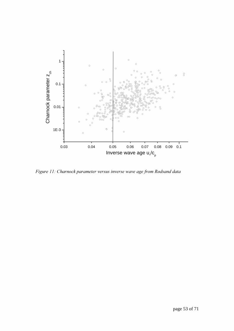
401 records (7% of the total number of records) are left in the final data set.

page 19 of 71

3 Observed trend in sea roughness

3.1 Trend of sea roughness with wave age

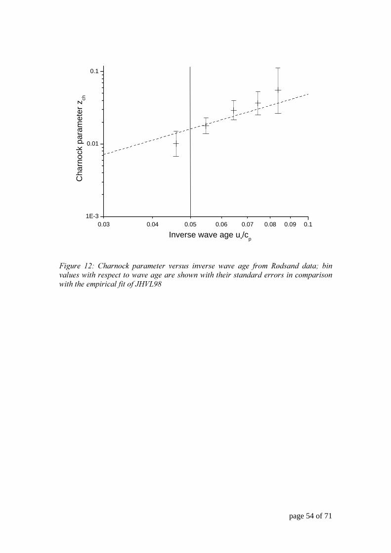
Figure 11 gives an overview over the data. The Charnock parameter is plotted versus

inverse wave age for all half-hourly records.

A bin-averaging method is used for trend investigation. First the data are sorted for

the value of the inverse wave age in bins. The bin width is 0.01. Afterwards averages

of u10n, u* and u*/cp are calculated for the records in each bin. The bin values of zch are

derived from the averaged parameters for each bin (see section 5 for a discussion of

the bin-averaging method). The standard errors of u10n and u* have been used to

estimate a standard error of the bin value of zch. Figure 12 shows a comparison of the

bin values with the wave age dependent relation for the Charnock parameter from

JHVL98. Bearing in mind the measurement uncertainties, the agreement is good.

However, from the error bars it can be seen that the scatter in the data is too large to

allow a quantification of the parameters in a power law. This can only be done by

using a data set with larger wave age variation as shown in section 3.4.

Only one bin value is available for inverse wave ages below the flow roughness limit

of 0.05, e.g. in the range where the trend might be influenced by smooth flow after the

Toba et al., (1990) criterion. The value does not show a significant deviation from the

observed general trend.

page 20 of 71

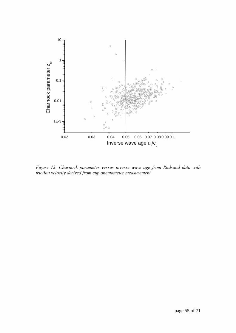
3.2 Trend obtained from cup anemometer measurements

With a sonic anemometer the wind stress can be measured with the well-established

eddy-correlation method. Omnidirectional sonic anemometers as the one used at

Rødsand are, however, susceptible to flow distortion errors especially in the vertical

wind speed component and therefore in the friction velocity. Flow distortion errors

are by their nature wind direction dependent. A concern is therefore that they coincide

with a wind direction dependent variation of wave age values due to different fetch

lengths. This could distort or even cause the observed trend of sea surface roughness

with wave age.

To rule out this threat, the friction velocity has also been derived by an alternative

indirect method from cup anemometer measurements (see section 2.3.1). The method

requires that the marine boundary layer is in an equilibrium condition. This can be

assumed for the data with near neutral stratification and nearly stationary conditions

used in this analysis. This method is expected to be less accurate than the direct eddy-

correlation method, but has the advantage of ruling out wind direction dependent flow

distortion errors.

Data have been analysed as before, only with the friction velocity derived from the

cup anemometer at 10 m height instead of that of the sonic anemometer. No selection

has been made for low friction velocities, since the measurement height of 10 m can

be expected to be always in the surface layer. The resulting data are shown in Figure

13 as Charnock parameter versus inverse wave age. The data have been bin-averaged

as described in section 3.1. Figure 14 shows the result in comparison with the result

obtained from the sonic anemometer and the relation proposed by JHVL98. The result

from the analysis of the cup anemometer data supports the trend found from the sonic

anemometer.

page 21 of 71

3.3 Trend obtained for different fetch lengths

The measurement location experiences fetches in a wide range from 10 km to more

than 100 km (see Figure 1). To test a possible dependence of the relation between

Charnock parameter and inverse wave age, four wind direction sectors with

approximately uniform fetches have been selected (Table 2).

This requires the selection of the data for narrow wind direction sectors. The wind

direction dependent flow distortion error of the sonic anemometer would in this case

distort the results, since the Charnock parameter is very sensitive to a bias in friction

velocity (an error of 8% in friction velocity causes a doubling of the Charnock

parameter). Therefore the friction velocity derived from the cup anemometer has been

used (see section 2.3.1). The data have been analysed as described in section 3.2.

The bin values of the Charnock parameter are plotted against inverse wave age for

each wind direction sector (see Figure 15). The trend of increasing Charnock

parameter with inverse wave age is generally confirmed, although with larger

variations. These are caused by the low number of measurement data available in each

wind direction sector (see Table 2). A systematic variation of the relation with fetch

length is not visible, i.e. a dependence of the coefficients of the power law relation

between Charnock parameter and inverse wave age on fetch length can not be found.

3.4 Trend obtained for an aggregated data set

The range of inverse wave age available at one measurement site is relatively small

(in the Rødsand data set typically 0.04 < u*/cp < 0.09). This, together with the

considerable scatter in the data, makes the determination of the parameters of a power

law relation unreliable. Following JHVL98, measurement data from different

page 22 of 71

locations and with a wide range of wave age values have therefore been combined in

an aggregated data set. Data compiled in Donelan et al. (1993) have been used.

For each data set the median values of Charnock parameter and inverse wave age

have been plotted (Figure 16). The median has been used as an approximation to the

bin values from averaged measured quantities, since the measured quantities were not

available individually. It can be seen that the result for the Rødsand measurement is

close to the trend line proposed by JHVL98.

A comparison with other proposed trend lines in the literature (Toba et al. (1990),

Drennan et al. (2003), Maat et al. (1991), Monbaliu (1994), Smith et al. (1992)) is

made in Figure 17. It can be seen that a wide range of coefficients has been found for

the power law relation zch=A(u*/cp)B. (see Table 3). Some possible reasons for these

differences are discussed in the following chapter.

4 Influence of self-correlation

In Hicks (1981) a numerical method is described to investigate the functional

relationship introduced by self-correlation. A functional relation is derived from an

artificial random ‘data’ set of unrelated values for the input parameters to the analysis.

The functional relationship found will solely be a result of the correlation introduced

in the analysis. Here the question is if the introduction of a quantity describing the

wave field, namely the wave phase speed as the only wave parameter in the relation,

leads to a relation between Charnock parameter and wave age, which has physical

meaning and is not a mere result of self-correlation.

For this purpose an artificial ‘data set’ has been produced, where the measured values

of wave phase speeds are exchanged by random numbers. Instead of a uniformly

page 23 of 71

distributed probability of the values as proposed by Hicks (1981), the probability

distribution is chosen to follow those of the measured data set (Figure 18c). This is

done by randomly redistributing the measured data of wave phase speed within the

data set. To increase the data volume and improve ‘randomness’ the measured data set

has been repeated several times. For friction velocity and neutral 10 m wind speed the

actual measurement values are used without change. Figure 18a and b show their

probability distributions in the Rødsand data set.

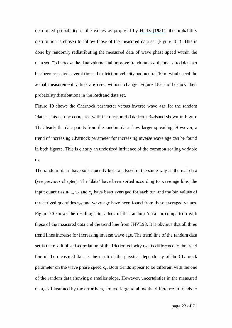
Figure 19 shows the Charnock parameter versus inverse wave age for the random

‘data’. This can be compared with the measured data from Rødsand shown in Figure

11. Clearly the data points from the random data show larger spreading. However, a

trend of increasing Charnock parameter for increasing inverse wave age can be found

in both figures. This is clearly an undesired influence of the common scaling variable

u*.

The random ‘data’ have subsequently been analysed in the same way as the real data

(see previous chapter): The ‘data’ have been sorted according to wave age bins, the

input quantities u10n, u* and cp have been averaged for each bin and the bin values of

the derived quantities zch and wave age have been found from these averaged values.

Figure 20 shows the resulting bin values of the random ‘data’ in comparison with

those of the measured data and the trend line from JHVL98. It is obvious that all three

trend lines increase for increasing inverse wave age. The trend line of the random data

set is the result of self-correlation of the friction velocity u*. Its difference to the trend

line of the measured data is the result of the physical dependency of the Charnock

parameter on the wave phase speed cp. Both trends appear to be different with the one

of the random data showing a smaller slope. However, uncertainties in the measured

data, as illustrated by the error bars, are too large to allow the difference in trends to

page 24 of 71

be conclusive, i.e. due to self-correlation not even the existence of a physical

dependency between Charnock constant and wave age can be deduced from this data

set. This confirms the conclusion of JHVL98, that a trend which is not severely

influenced by self-correlation can only be found when an aggregated data set is used.

The range of wave age values has to be large enough to allow a statistically

significant separation between the observed trend line and the trend line obtained

without wave information.

Ideally, the self-correlation should be investigated for the aggregated data set used in

section 3.4. The measured quantities of these data sets were not available. Instead, a

smaller sub-set of the Rødsand data are used to investigate the effect of different data

sets on self-correlation. For this only data with a nearly constant wave phase speed cp

of 6±0.2m/s have been selected. The analysis of the data as well as the compilation

and analysis of a simulated random ‘data’ set has been repeated and compared with

the result of all data (Figure 21). The Charnock parameters found from the subset of

measured data with nearly constant cp is slightly lower, while the steepness of the

relation remains largely unchanged. This is different for the randomised 'data'.

Obviously, randomising cp in a data subset where it is nearly constant does not lead to

significant changes and the trend of Charnock parameter with inverse wave age for

the randomised 'data' is the same as for the measured data, i.e. the relation is

completely determined by self-correlation. Using all measured data, e.g. the whole

range of cp values available at this particular site (see Figure 18), the difference

between measured and randomised data in the trends of Charnock parameter versus

inverse wave age becomes larger. However, as mentioned above the range of cp

values is not wide enough to allow a statistically significant separation of both trends

for the Rødsand data set. For a data set with a very wide range of cp values, which

page 25 of 71

could be obtained by aggregating data from different sites, it can be expected that the

trends of measured and randomised data are more separated. In this way the effect of

self-correlation could be separated from the physical dependency between Charnock

constant and wave age.

5 Discussion of analysis method

5.1 Bin-averaging

For the dependence of the Charnock parameter on inverse wave age a power law

relation is assumed. The coefficients of the relation have to be found empirically by a

fit to measured data. A problem arises if the data show a large statistical spreading

and one of the scaling groups does not follow a normal probability distribution.

Data of measured Charnock parameters have a large spreading, mainly due to the

sampling variability in the u* measurement. Also, the Charnock parameter depends on

physical quantities of u* and u10n in a highly non-linear way (see equation 7).

Therefore it can not be simply averaged and a fit based on a rms-error of zch does not

seem suitable. A simple example: Assuming 3 records with u10n of 10 m/s and u* of

0.2, 0.3 and 0.4 m/s the zch values are calculated to 0.000005, 0.001 and 0.03. The

average of the zch values is 0.01. If instead the physical measured quantities are

averaged and zch is calculated from the average u10n and u* values, the average zch is

0.001, i.e. an order of magnitude smaller.

To avoid these problems, a bin-averaging method is used instead of a direct fit or an

averaging of zch. The procedure generally consists of two steps: First the data are

page 26 of 71

sorted for the value of one parameter (sorting parameter) in bins. Afterwards one or

several parameters are averaged over all records in each bin (averaged parameters)

and derived quantities are calculated from these (bin values). In the resulting bin

values the large statistical spreading has vanished and a linear fit can be made to

determine the coefficients of the power law relation. For the determination of a power

law relation between Charnock parameter and inverse wave age, the inverse wave age

is used as sorting parameter. The averaged parameters are the measured quantities u*,

u10n and cp. The Charnock parameter is then calculated from these averaged values for

each bin. As an estimate of the measurement uncertainty, standard errors of zch are

calculated from the standard errors of the averaged quantities.

Figure 22 shows the difference between the fits of a power law relation to the

measured Charnock parameters and the bin values. The large difference is obvious.

Also shown is the result of a fit to the logarithm of the measured Charnock parameter

log10(zch). It can be seen that this is a good approximation to the bin-averaging

method.

In the previous chapter it was found that the trend of the Charnock parameter with

inverse wave age is influenced or even determined by the self-correlation due to the

variability in u*, depending on the range of the u* and cp values in the data set. Since

this self-correlation is part of the relation found from the measured data, it will also

differ for different data sets. This partly explains the differences found from different

data sets for the coefficients of the power law relation. The effect of different data sets

on the relation found is shown again in Figure 23 for three different wind speed

intervals. The data have been sorted according to wind speed and inverse wave age in

a two-dimensional bin averaging. The small squares show the bin values of Charnock

parameter versus inverse wave age for a certain wind speed and inverse wave age

page 27 of 71

interval. It is found that the relation is steeper for a narrow wind speed interval due to

the dominating influence of self-correlation in u*. Figure 23 also shows how the

choice of the sorting parameter can influence the result of the trend investigation. The

large squares are the bin values for the three wind speed intervals without sorting for

inverse wave age. The different sorting parameter, in this case wind speed, leads to a

different apparent trend of Charnock parameter with inverse wave age.

5.2 Rough flow condition

One of the conditions for the dependence of sea surface roughness on wave age alone

is that the air flow must be rough turbulent (see JHVL98). If this condition is not

satisfied, it can be expected that the sea surface roughness would also depend on the

Reynolds roughness number of the flow.

JHVL98 and others (e.g. Drennan et al.,2003) follow Toba et al. (1990) in defining a

limiting roughness Reynolds number Rcr=u*z0/ν (with ν=kinematic viscosity) for fully

rough flow of 2.3. Since the value is important for the selection of data an attempt is

made to uncover its origins in the literature. Toba et al. (1990) quote Schlichting

(1979), who defines aerodynamically fully rough flow by:

70>∗

νV��

(15)

here ks is the sand grain size used in experiments in rough pipes by Nikuradse (1933).

For other flows this is related to the roughness parameter k by the empirically found

formula by Schlichting (1936):

���

V −=

5.8log75.5 10 (16)

page 28 of 71

Concerning the flow of natural winds over the surface of the earth, Schlichting reports

findings from Paeschke (1937), who found B=5 when the physical height of the

vegetation is used as roughness parameter k. This leads to the relation ks=4k between

Nikuradse’s sand grain size ks and the roughness parameter k. The logarithmic profile

used by Schlichting:

���

�� +

=

∗

ln5.2 (17)

can be used to relate his roughness parameter k to the surface roughness length z0.

Inserting the result, k=7.4 z0, and ks=4k in equation 17 leads to the limiting roughness

Reynolds number used by JHVL98 and Toba et al. (1990):

3.20 == ∗

�

�FU

(18)

Kitaigorodskii (1970) takes a similar approach also based on the measurements of

Nikuradse (1933) and finds a similar limiting value of 3.0. The many assumptions

about the similar behaviour of flow through pipes and in the atmosphere and about the

similar effect of sand, vegetation and waves suggest that these values should be used

with caution.

In the following it is shown that the application of the roughness Reynolds number as

roughness criterion in a data set with large scatter can lead to a misleading impression

about the overall trend in a zch versus u*/cp plot depending on the effective fetch of the

site. This is caused by the large scatter of the measured sea surface roughness, which

enters into the selection criterion as part of the flow roughness.

The rough flow condition can be written in terms of the Charnock parameter as:

3*−> ����

FUFKν (19)

page 29 of 71

where Rcr= z0u*/ν is the critical flow roughness for rough turbulent flow. For growing

wind-waves in fetch limited cases in deep water, Kahma and Calkoen (1994) obtained

the following relationship:

54.0*

27.0* )(08.3 �����

S

−= (20)

Equations 20 and 21 can be combined to give:

56.5

*5.1)(4.520

−

−

>

S

FUFK ��

����� ν (21)

Equation 23 is the roughness flow condition expressed in terms of the dimensionless

sea roughness (Charnock parameter), inverse wave age and fetch. On a zch versus

u*/cp plot, this condition filters out all data points below the line given by Equation

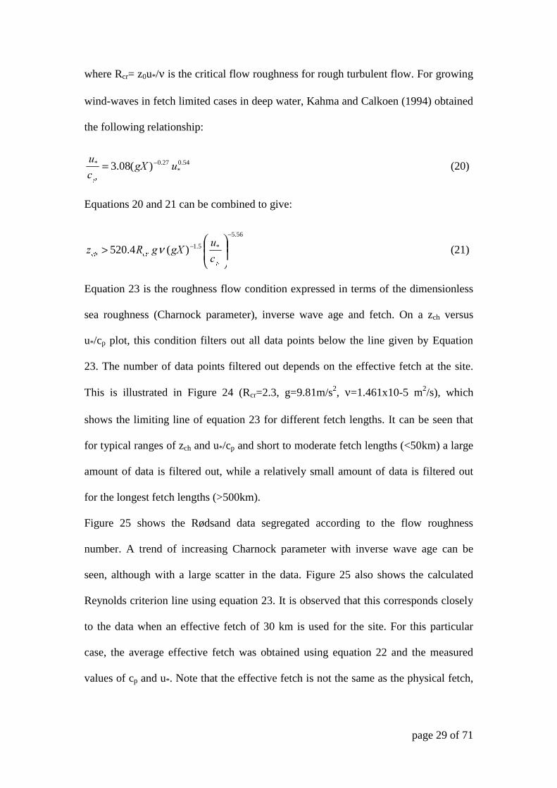
23. The number of data points filtered out depends on the effective fetch at the site.

This is illustrated in Figure 24 (Rcr=2.3, g=9.81m/s2, ν=1.461x10-5 m2/s), which

shows the limiting line of equation 23 for different fetch lengths. It can be seen that

for typical ranges of zch and u*/cp and short to moderate fetch lengths (<50km) a large

amount of data is filtered out, while a relatively small amount of data is filtered out

for the longest fetch lengths (>500km).

Figure 25 shows the Rødsand data segregated according to the flow roughness

number. A trend of increasing Charnock parameter with inverse wave age can be

seen, although with a large scatter in the data. Figure 25 also shows the calculated

Reynolds criterion line using equation 23. It is observed that this corresponds closely

to the data when an effective fetch of 30 km is used for the site. For this particular

case, the average effective fetch was obtained using equation 22 and the measured

values of cp and u*. Note that the effective fetch is not the same as the physical fetch,

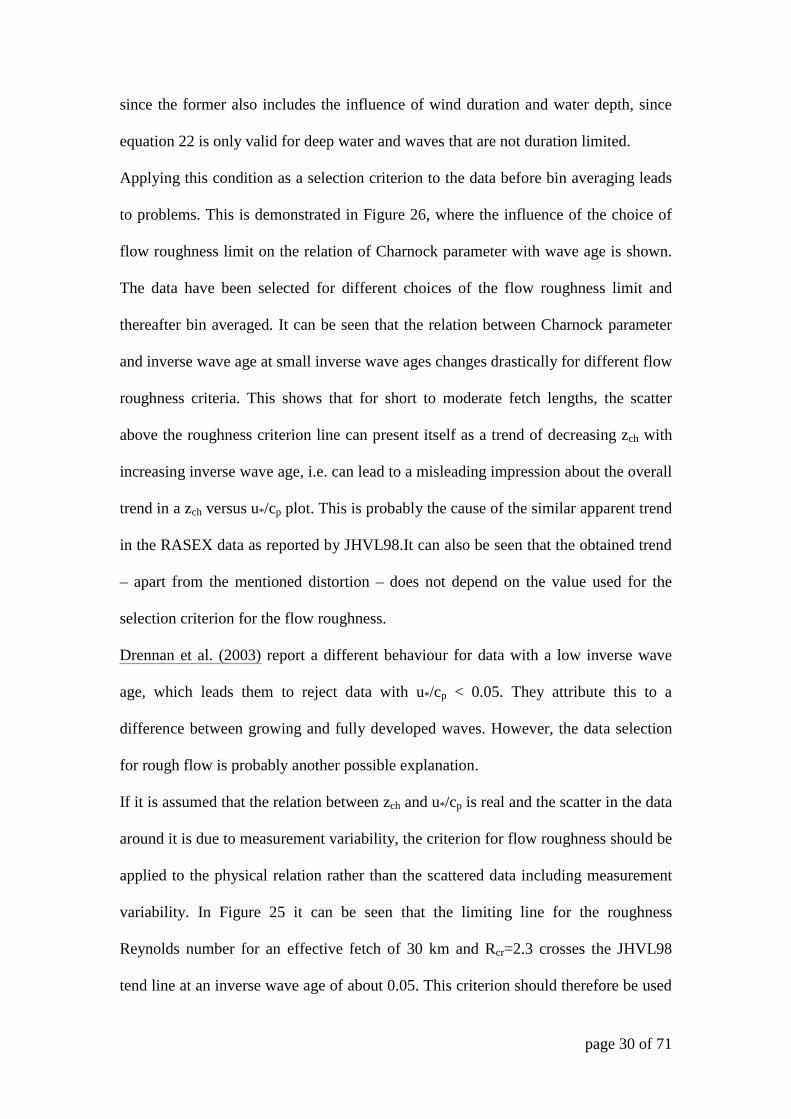
page 30 of 71

since the former also includes the influence of wind duration and water depth, since

equation 22 is only valid for deep water and waves that are not duration limited.

Applying this condition as a selection criterion to the data before bin averaging leads

to problems. This is demonstrated in Figure 26, where the influence of the choice of

flow roughness limit on the relation of Charnock parameter with wave age is shown.

The data have been selected for different choices of the flow roughness limit and

thereafter bin averaged. It can be seen that the relation between Charnock parameter

and inverse wave age at small inverse wave ages changes drastically for different flow

roughness criteria. This shows that for short to moderate fetch lengths, the scatter

above the roughness criterion line can present itself as a trend of decreasing zch with

increasing inverse wave age, i.e. can lead to a misleading impression about the overall

trend in a zch versus u*/cp plot. This is probably the cause of the similar apparent trend

in the RASEX data as reported by JHVL98.It can also be seen that the obtained trend

– apart from the mentioned distortion – does not depend on the value used for the

selection criterion for the flow roughness.

Drennan et al. (2003) report a different behaviour for data with a low inverse wave

age, which leads them to reject data with u*/cp < 0.05. They attribute this to a

difference between growing and fully developed waves. However, the data selection

for rough flow is probably another possible explanation.

If it is assumed that the relation between zch and u*/cp is real and the scatter in the data

around it is due to measurement variability, the criterion for flow roughness should be

applied to the physical relation rather than the scattered data including measurement

variability. In Figure 25 it can be seen that the limiting line for the roughness

Reynolds number for an effective fetch of 30 km and Rcr=2.3 crosses the JHVL98

tend line at an inverse wave age of about 0.05. This criterion should therefore be used

page 31 of 71

by rejecting data with lower inverse wave ages. In this way the distortion of the result

due to application of a selection criterion to a scattered data set is avoided.

An approach different from that used by Toba et al. (1990) and Kitaigorodskii (1970)

is proposed by Donelan (1990), who summarises open ocean experiments from Smith

(1980) and Large and Pond (1981). He distinguishes only between smooth and rough

flow and used the friction velocity as criterion for flow roughness:

*0 11.0

��

ν= for

( )��

�� 1.02 31

* =< ν (smooth flow) (22)

��

�2

*0 014.0=

for ( )

��

�� 1.02 31

* => ν (rough flow) (23)

The limit for u* is the value where the sea surface roughness for smooth and

rough flow are equal. For the Rødsand data this criterion is automatically fulfilled

since data with u*<0.2 m/s have been rejected already to ensure that the sonic

anemometer is in the surface layer (see section 2.5).

6 Conclusion

New simultaneously measured wind and wave data from the field measurement

program at Rødsand in the Danish Baltic Sea are presented. These data have been

used to test the wave age dependence of the Charnock parameter (or dimensionless

sea surface roughness). A general trend of increasing sea roughness with inverse wave

age is obtained which agrees with the trend found in JHVL98 and similar

parameterisations.

However, by analysing a simulated data set of randomly generated wave ‘data’ it was

shown that self-correlation severely influences the observed relation between

page 32 of 71

Charnock parameter and wave age. Uncertainties in the measured data are too large to

allow the difference in trends between real and simulated random ‘data’ to be

conclusive. This means that with the Rødsand data set alone, not even the existence of

a physical dependency between Charnock parameter and wave age can be proven.

By using a small sub-set of the Rødsand data it was shown that for a data set with a

narrow range of cp the trend lines of real and random 'data' become almost identical.

The larger the range in cp values, the less significant is the influence of self-

correlation. In other words, the wave age variation needs to be caused by the variation

in cp, not by the spreading in u*. We believe that for a data set with a very large range

of wave age values the influences of self-correlation and physical dependency can be

separated. This supports the basic idea of JHVL98, that a trend, which is not severely

influenced by self-correlation, can only be found with an aggregated data set where

the range of wave phase speed values is large. Further research is needed here.

From this investigation it becomes clear that the dependence of the Charnock

parameter on wave age is less pronounced than what could be expected without taking

into account the influence of self-correlation. We therefore expect that, even if the

physical nature of the trend can be shown with such an aggregated data set, the

improvement of the Charnock relation with a wave age dependent Charnock

parameter is limited. Future research should consider also alternative approaches for

the parameterisation of the Charnock parameter, e.g. with wave height or wave

steepness.

In the literature, different coefficients for the power law between Charnock parameter

and wave age have been found for different data sets. Such differences can be

expected since for different data sets – and hence different ranges of the quantities u*

page 33 of 71

and cp – different self-correlation relations follow, which lead to different coefficients

in the power law relation.

Additionally, it is shown that the roughness Reynolds number criterion often applied

to select data with rough turbulent flow can lead to a misleading impression about the

trend in the data, since the sea surface roughness is present in both the selection rule

and in the quantity under investigation. This is believed to be the cause of the

apparent trend of a decrease in Charnock parameter with inverse wave age in the

RASEX data as reported by JHVL98. The importance of this distortion varies with the

effective fetch length at the site. It is mainly important for short to medium fetch

lengths. Two alternative methods to ensure aerodynamically rough flow are discussed,

which do not distort the relation. Instead of applying the roughness Reynolds number

criterion to the (scattered) data it can be applied to the relationship found. This leads

to a limiting inverse wave age, which in the case of the Rødsand data is u*/cp>0.05. A

different criterion for rough flow is the one by Donelan (1990), who finds a limit of

u*>0.1m/s for rough flow, by equating the sea surface roughness estimated for rough

and smooth flow.

A misleading trend can also be caused by the methods to obtain the parameterisation

from the data. Investigation of the bin-averaging method showed that the choice of the

sorting parameter in the bin-averaging analysis can lead to an inversion of the

observed trend of Charnock parameter with wave age.

To sum up, we conclude that the parameterisation of the Charnock parameter as a

function of wave age is fraught with many difficulties, hence one must be cautious in

using such a relationship, especially if derived from single site measurements. Some

of the difficulties include the influence of self-correlation, selective filtering

introduced by the roughness flow condition, and the usually large scatter in the

page 34 of 71

Charnock parameter itself. Some of the differences found in the literature can

probably be explained by these difficulties.

The Rødsand data show an increase of Charnock parameter with inverse wave age in

line with most literature results. While the existence of the trend seems clear, the

significance of it is not. We find that the importance of the physical dependency in the

Rødsand data set is questioned by self-correlation effects, i.e. that the relation is

severely influenced by self-correlation. However, our results point to that the self-

correlation effects can be reduced by striving for an equally strong variability of the

different data entering into the regression procedure and taking effort to avoid for

spurious correlation between the parameters, as for example by aggregating data sets

as in JHVL98.

Acknowledgements

The research was funded by the Danish Technical Research Council (STVF) as part

of the project “Wind-wave interaction in coastal and shallow areas”. We gratefully

acknowledge the financial support of the Rødsand measurement program by the

following: European Union, JOULE program (JOU2-CT93-0325), Office of naval

research (N00014-93-1-0360) and ELKRAFT. The work of one of the authors (B.

Lange) was partly funded by the European Commission through a Marie Curie

Research Training Grant. Many tanks to Rebecca Barthelmie from Risø for managing

the Rødsand field experiment since 1998. The technical support team at Risø and Mr

Kobbernagel of Sydfalster-El are acknowledged for their contribution to the data

collection. The authors wish to thank the reviewersfor their important and useful

comments, which led to a substantial improvement of the paper.

page 35 of 71

References

Charnock, H., 1955: Wind stress over a water surface. ����������������������, ��,

639-640.

Donelan, M., 1990: Air-sea interaction. ���!"!�#!���#!���#�!��$�%���&'�����

(����, B. Le Méhauté and D.M. Hanes, Eds., 239-292.

Donelan, M.A., F.W. Dobson, S.D. Smith and R.J. Anderson, 1993: On the

dependence of sea surface roughness on wave development. �� '(���

���!����, ��, 2143-2149.

Drennan, W. M., H. C. Graber, D. Hauser and C. Quentin, 2003: On the wave age

dependence of wind stress over pure wind seas ��)��*(��� ����, ��� (C3),

8062.

Garratt, J.R., 1992: (� �����*(��#� ���!+��� %����. Cambridge University Press,

316pp.

Geernaert, G.L., K.B. Katsaros and K. Richter, 1986: Variation of the drag coefficient

and its dependence on sea state. ��)��*(�������, ��, 7667-7679.

Hasselmann, K., T. P. Barnett, E. Bouws, H. Carlson, D. E. Cartwright, K. Enke, J. A.

Ewing, H. Gienapp, D. E. Hasselmann, P. Kruseman, A. Meerburg, P. Müller,

D. J. Olbers, K. Richter, W. Sell and H. Walden, 1973: Measurements of

Wind-Wave Growth and Swell Decay during the Joint North Sea Wave

Project (JONSWAP). Dtsch. Hydrogr. Z. Suppl., A 12, No.8

Hicks, B.B., 1978: Some limitations of dimensional analysis and power laws. ���!+�,

�����������- ��, 567-569.

Hicks, B.B., 1981: An examination of turbulence statistics in the surface boundary

layer. ���!+�,����������., ��, 389-402.

page 36 of 71

Hsu, S.A., 1974: A dynamic roughness equation and its application to wind stress

determination at the air-sea interface. ��'(��� ���!����, �, 116-120.

Højstrup, J., 1999: Vertical Extrapolation of Offshore Windprofiles. .#!+�!�������

�(� !�/� �#%%�!!#��. Proceedings. 1999 European wind energy conference

(EWEC '99), Nice (FR). Petersen, E.L.; Hjuler Jensen, P.; Rave, K.; Helm, P.;

Ehmann, H., Eds., 1220-1223.

Johnson, H.K., J. Højstrup, H.J. Vested, S.E. Larsen, 1998: On the dependence of sea

surface roughness on wind waves. ��'(��� ���!���., ��, 1702-1716.

Kahma, K.K. and C.J. Calkoen, 1994: Growth curve observations. 0�!��#�� �!+

��+�%%#!� �� ���! .����- G.J. Komen, L. Cavaleri, M Donelan, K.

Hasselmann, S. Hasselmann, P.A.E.M. Janssen, Cambridge University Press,

174-182.

Kitaigorodskii, S.A., 1970: (�*(��#�����#�,���#!������#�!� ��!�%���+����

����#�!���������(, Israel Program for Scientific Translations, Jerusalem,

237pp.

Lange, B., R.J. Barthelmie and J. Højstrup, 2001: 0����#*�#�! �� �(��1+��!+ �#�%+

���������!�� Report Risø-R-1268. Risø National Laboratory, DK-4000

Roskilde, Denmark, 59pp. (available on www.risoe.dk)

Large, W.G. and S. Pond, 1981: Open ocean momentum flux measurements in

moderate to strong winds. ��'(��� ���!���., ��, 464-482.

Maat, N., C. Kraan and W. A. Oost, 1991: The roughness of wind waves. ���!+���,

�����������%���, ��, 89-103.

Monbaliu, J., 1994: On the use of the Donelan wave spectral parameter as a measure

for the roughness of wind waves. ���!+���,�����������%�, , 277-291.

page 37 of 71

Mortensen, N.G. and J. Højstrup, 1995: The solent sonic – response and associated

errors. '�����+#!�� �� �(� &�( ��� ���*��#�� �! �������%��#��%

��������#�!� �!+ #!������!���#�!, March 27-31, 1995, Charlotte, N.C.,

pp.501-506; AMS, Boston, Massachusetts

Nikuradse, J., 1933.: Strömungsgesetze in rauhen Röhren. 2����(�� ���� 3!��,.���

No. 361.

Paeschke, W., 1937: Experimentelle Untersuchungen zum Rauhigkeits- und

Stabilitätsproblem in der bodennahen Luftschicht, Dissertation, Universität

Göttingen.

Schlichting, H., 1936: Experimentelle Untersuchungen zum Rauhigkeitsproblem.

3!��,���(., , 1-34Schlichting, H.,1979: ���!+���,���� (����. Seventh

edition. McGraw-Hill, New York, 817 pp.

Schlichting, H., 1979: ���!+���,���� (����� McGraw-Hill, New York; 817 pp.

Schotanus, P., F. T. M. Nieuwstadt and H. A. R. De Bruin, 1983: Temperature

measurement with a sonic anemometer and its application to heat and moisture

fluxes. ���!+�,�����������, �, 81-93.

Smith, S.D., 1980: Wind stress and heat flux over the open ocean in gale force winds.

��'(��� ���!���.,��, 709-726.

Smith, S.D., R.J. Anderson, W.A. Oost, C. Kraan, N. Maat, J. DeCosmo, K.B.

Katsaros, K.L. Davidson, K. Bumke, L. Hasse, and H.M. Chadwick, 1992: Sea

surface wind stress and drag coefficients: The HEXOS results. ���!+�,����

�������, �, 109-142.

Stull, R. B., 1988: �!#!���+���#�!�����!+���%�����������%����Kluwer Academic

Publishers, 666pp.

page 38 of 71

Taylor, P.K., M.J. Yelland, 2001: The dependence of sea surface roughness on the

height and steepness of the waves. ��'(��� ���!���., ��, 572-590.

Tennekes, H., 1982: Similarity relations, scaling laws and spectral dynamics.

�����*(��#� �����%�!�� �!+�#�*�%%��#�!��+�%%#!�, F.T.M. Nieuwstadt and

H. van Dop, Eds., Reidel, pp.37-68.

Toba, Y., N. Iida, h. Kawamura, N. Ebuchi and I.S.F. Jones, 1990: Wave dependence

on sea-surface wind stress, ��'(��� ���!���., 20, 705-721.

Wyngaard, J. C., 1973: On surface-layer turbulence. .����(�*�!�#����������%���.

D. A. Haugen, Ed., American Meteorological Society, Boston, pp. 101-149.

Yelland, M. J. and P. K. Taylor, 1996: Wind stress measurements from the Open

Ocean, ��'(��� ���!���., 26, 541-558.

page 39 of 71

Figure captions Figure 1: Rødsand measurement site

Figure 2: Ratio of standard deviation measured with the cup anemometer at 50 m

height and friction velocity derived from the sonic anemometer at 46.6 m (42.3

m) height versus stability parameter 50/L; horizontal lines show the mean ratio

(2.42) and its standard deviation (0.51)

Figure 3: Ratio of standard deviation measured with the cup anemometer at 50 m

height and friction velocity derived from the sonic anemometer at 46.6 m (42.3

m) height versus inverse wave age u*/cp; horizontal lines show the mean ratio

(2.42) and its standard deviation (0.51)

Figure 4: Bandwidth of the measured data at Rødsand versus significant wave height;

also shown is the bandwidth of the fitted JONSWAP spectrum (0.15) and the

bandwidth limit used to select single peaked spectra (0.25)

Figure 5: Ratio of mean period and wave period based on zero crossing frequency of

the measured data at Rødsand versus significant wave height; also shown is the

timescale ratio of the fitted JONSWAP spectrum

Figure 6: Difference between friction velocities derived from cup anemometer

standard deviations at 10 m and 50 m height versus stability parameter;

horizontal lines show the mean difference (0.036 m/s), its standard deviation

(0.029 m/s) and the mean result of eq. (13)

Figure 7: Difference between friction velocities derived from cup anemometer

variances at 10 m and 30 m height versus stability parameter; horizontal lines

show the mean difference (0.021 m/s), its standard deviation (0.019 m/s) and the

mean result of eq. (13)

page 40 of 71

Figure 8: Triangles: Binned ratios of wind speed measurements at 38m . Circles:

Model results assuming flow distortion linear away from tower wake influence

(see also Figure 9); data are from the Vindeby measurement program

Figure 9: Correction for tower flow distortion of wind speed at Rødsand as a function

of wind direction with the model by Højstrup (1999). Note that the correction is

positive on average, and that the correction diminishes for increasing boom

length to tower side ratio

Figure 10: Triangles: Binned ratios of measurements of wind speed standard

deviations at 38m . Circles: Model results assuming flow distortion linear away

from tower wake influence; data are from the Vindeby measurement program

Figure 11: Charnock parameter versus inverse wave age from Rødsand data

Figure 12: Charnock parameter versus inverse wave age from Rødsand data; bin

values with respect to wave age are shown with their standard errors in

comparison with the empirical fit of JHVL98

Figure 13: Charnock parameter versus inverse wave age from Rødsand data with

friction velocity derived from cup anemometer measurement

Figure 14: Charnock parameter versus inverse wave age from Rødsand data with

friction velocity derived from cup and sonic anemometer measurements; bin

values with respect to wave age are shown with their standard errors in

comparison with the empirical fit of JHVL98

Figure 15: Charnock parameter versus inverse wave age from Rødsand measurement

bin averaged with respect to wave age; data from four wind direction sectors

with different fetches are shown together with the empirical fit of JHVL98

Figure 16: Scatter plot of averaged Charnock parameter versus inverse wave age for

several data sets and comparison with the empirical fit of JHVL98

page 41 of 71

Figure 17: Comparison of averaged Charnock parameter versus inverse wave age for

several data sets with proposed empirical relations

Figure 18: Probability distributions of u*, u10n, and cp in the measured Rødsand data

Figure 19: Charnock parameter versus wave age from simulated random ‘data’

Figure 20: Wave age bin values of Charnock parameter versus inverse wave age from

the Rødsand measurement and the simulated random ‘data’; also shown is the

JHVL98 relation

Figure 21: Comparison of wave age dependency of Charnock parameter for all data

and a data subset with wave phase speed cp of 6±0.2 m/s; shown are results from

the Rødsand measurement and simulated random ‘data’ sets

Figure 22: Comparison of methods to fit a power law relation between Charnock

parameter and inverse wave age to measured data

Figure 23: Charnock parameter versus wave age from Rødsand measurement; bin

values from bin averaging with respect to inverse wave age (large triangles) and

with respect to neutral wind speed at 10 m height (large squares) are shown as

well as bin values after the data were sorted and bin averaged both in wind speed

and inverse wave age bins (small squares)

Figure 24: Sensitivity of the roughness flow criterion of JHVL98 with fetch on a plot

of Charnock parameter versus inverse wave age (Rcr=2.3); based on equation 23

Figure 25: Charnock parameter versus inverse wave age from Rødsand data

segregated according to flow roughness; also shown are the limiting lines of

equation 23 for an effective fetch of 30 km and a Rcr of 2.3, 0.5 and 0.1

Figure 26: Charnock parameter versus inverse wave age for different flow roughness

selection criteria

page 42 of 71

Table captions Table 1��Instrumentation of the Rødsand measurement

Table 2: Selected wind direction sectors with approximately uniform fetch

Table 3: Parameter values proposed for the power law relation zch=A(u*/cp)B in the

literature

page 43 of 71

50km

������

Denmark

Germany

2#����45�1+��!+���������!��#��

page 44 of 71

-0.5 -0.4 -0.3 -0.2 -0.1 0.0 0.1 0.2 0.30.0

0.5

1.0

1.5

2.0

2.5

3.0

3.5

4.0

4.5

5.0

5.5

6.0

6.5

σ u,cu

p50/

u *,so

nic

50/L

2#���� 65 ���#� �� ���!+��+ +��#��#�!�������+�#�( �(� ��* �!�������� �� 78�(�#�(� �!+ ��#��#�! ��%��#�� +��#��+ ���� �(� ��!#� �!�������� �� 9:�:� ;96�<�=(�#�(� ������ ����#%#�� *�������� 78>? (��#��!��% %#!�� �(�� �(����! ���#� ;6�96=�!+#�����!+��++��#��#�!;8�74=

page 45 of 71

0.03 0.04 0.05 0.06 0.07 0.08 0.09 0.100.0

0.5

1.0

1.5

2.0

2.5

3.0

3.5

4.0

4.5

5.0

5.5

6.0

6.5

σ u,cu

p50/

u *,so

nic

Inverse wave age u*/c

p

2#���� <5 ���#� �� ���!+��+ +��#��#�!�������+�#�( �(� ��* �!�������� �� 78�(�#�(� �!+ ��#��#�! ��%��#�� +��#��+ ���� �(� ��!#� �!�������� �� 9:�:� ;96�<�=(�#�(�������#!������������� >�S?(��#��!��%%#!���(���(����!���#�;6�96=�!+#�����!+��++��#��#�!;8�74=

page 46 of 71

0.0 0.2 0.4 0.6 0.8 1.0 1.2 1.4 1.6 1.8 2.00.00

0.05

0.10

0.15

0.20

0.25

0.30

0.35

0.40

selection limit

JONSWAP mean

Ban

dwid

th lo

g(f 75

/f 25)

Significant wave height Hs [m]

2#����95��!+�#+�(���(��������++������1+��!+�������#�!#�#��!�����(�#�(�?�%�� �(��! #� �(� ��!+�#+�( �� �(� �#���+ � @�.�' �*������ ;8�47= �!+ �(���!+�#+�(%#�#����+����%����#!�%�*����+�*�����;8�67=

page 47 of 71

0.0 0.2 0.4 0.6 0.8 1.0 1.2 1.4 1.6 1.81.00

1.02

1.04

1.06

1.08

1.10

1.12

1.14

1.16

1.18

1.20

Tim

esca

le r

atio

Tm/T

z

Significant wave height Hs [m]

2#����75���#������!*��#�+�!+����*��#�+����+�!���������#!����A��!�����(� �������+ +��� �� �1+��!+ ������ �#�!#�#��!� ���� (�#�(�? �%�� �(��! #� �(��#�����%����#����(��#���+� @�.�'�*������

page 48 of 71

-0.5 -0.4 -0.3 -0.2 -0.1 0.0 0.1 0.2 0.3-0.15

-0.10

-0.05

0.00

0.05

0.10

0.15

measured mean measured standard deviation Panofsky, 1973

u *,cu

p10

- u *,

cup5

0 [m

/s]

50/L

2#���� :5 0#�����!�� ������! ��#��#�! ��%��#�#�� +��#��+ ���� ��* �!�����������!+��++��#��#�!���48��!+78�(�#�(������� ����#%#��*��������?(��#��!��%%#!���(���(����!+#�����!��;8�8<:�>�=-#�����!+��++��#��#�!;8�86&�>�=�!+�(����!����%����A�;4<=

page 49 of 71

-0.5 -0.4 -0.3 -0.2 -0.1 0.0 0.1 0.2 0.3-0.15

-0.10

-0.05

0.00

0.05

0.10

0.15

measured mean measured standard deviation Panofsky, 1973

u *,cu

p10

- u *,

cup3

0 [m

/s]

50/L

2#���� B5 0#�����!�� ������! ��#��#�! ��%��#�#�� +��#��+ ���� ��* �!�����������#�!�����48��!+<8�(�#�(�����������#%#��*��������?(��#��!��%%#!���(���(� ���! +#�����!�� ;8�864 �>�=- #�� ���!+��+ +��#��#�! ;8�84& �>�= �!+ �(� ���!����%����A�;4<=

page 50 of 71

0 30 60 90 120 150 180 210 240 270 300 330 3600.90

0.92

0.94

0.96

0.98

1.00

1.02

1.04

1.06

1.08

1.10u3

8 Nor

th/u

38S

outh

wind direction

measurement model

2#���� C5 �#�!�%��5 �#!!�+ ���#�� �� �#!+ �*��+ ���������!�� �� <C� � �#��%��5��+�% ����%�������#!� �%��+#�����#�! %#!������� ���� ��������� #!�%��!�� ;����%��2#����&=?+�����������(�$#!+������������!�*������

page 51 of 71

0 45 90 1 35 180 225 27 0 315 3600.99

1.00

1.01

1.02

1.03

Flow through tower

10 m 30 m 50 m

Um

easu

red/U

true

Wind direction

2#����&5�������#�!���������%��+#�����#�!���#!+�*��+���1+��!+�����!��#�!�� �#!+ +#����#�! �#�( �(� ��+�% �� �1D����* ;4&&&=� @��� �(�� �(� �������#�! #�*��#�#���!�������-�!+�(���(��������#�!+#�#!#�(�����#!�����#!�����%�!��(��������#+����#�

page 52 of 71

0 30 60 90 120 150 180 210 240 270 300 330 3600.80

0.85

0.90

0.95

1.00

1.05

1.10

1.15

1.20

measurement model

sigm

a_u 38

_Nor

th/s

igm

a_u 38

_Sou

th

Wind direction

2#���� 485 �#�!�%��5 �#!!�+ ���#�� �� ���������!�� �� �#!+ �*��+ ���!+��++��#��#�!���<C���#��%��5��+�%����%�������#!��%��+#�����#�!%#!��������������������#!�%��!��?+�����������(�$#!+������������!�*������

page 53 of 71

0.03 0.04 0.05 0.06 0.07 0.08 0.09 0.1

1E-3

0.01

0.1

1

Cha

rnoc

k pa

ram

eter

zch

Inverse wave age u*/c

p

2#����445�(��!���*��������������#!�����������������1+��!++���

page 54 of 71

0.03 0.04 0.05 0.06 0.07 0.08 0.09 0.11E-3

0.01

0.1C

harn

ock

para

met

er z

ch

Inverse wave age u*/c

p

2#���� 465 �(��!��� *�������� ������ #!����� ���� ��� ���� �1+��!+ +���? �#!��%����#�(���*����������������(��!�#�(�(�#����!+��+������#!���*��#��!�#�(�(���*#�#��%�#�����$&C

page 55 of 71

0.02 0.03 0.04 0.05 0.06 0.07 0.08 0.09 0.1

1E-3

0.01

0.1

1

10

Cha

rnoc

k pa

ram

eter

zch

Inverse wave age u*/c

p

2#���� 4<5 �(��!��� *�������� ������ #!����� ���� ��� ���� �1+��!+ +��� �#�(��#��#�!��%��#��+��#��+������*�!�����������������!�

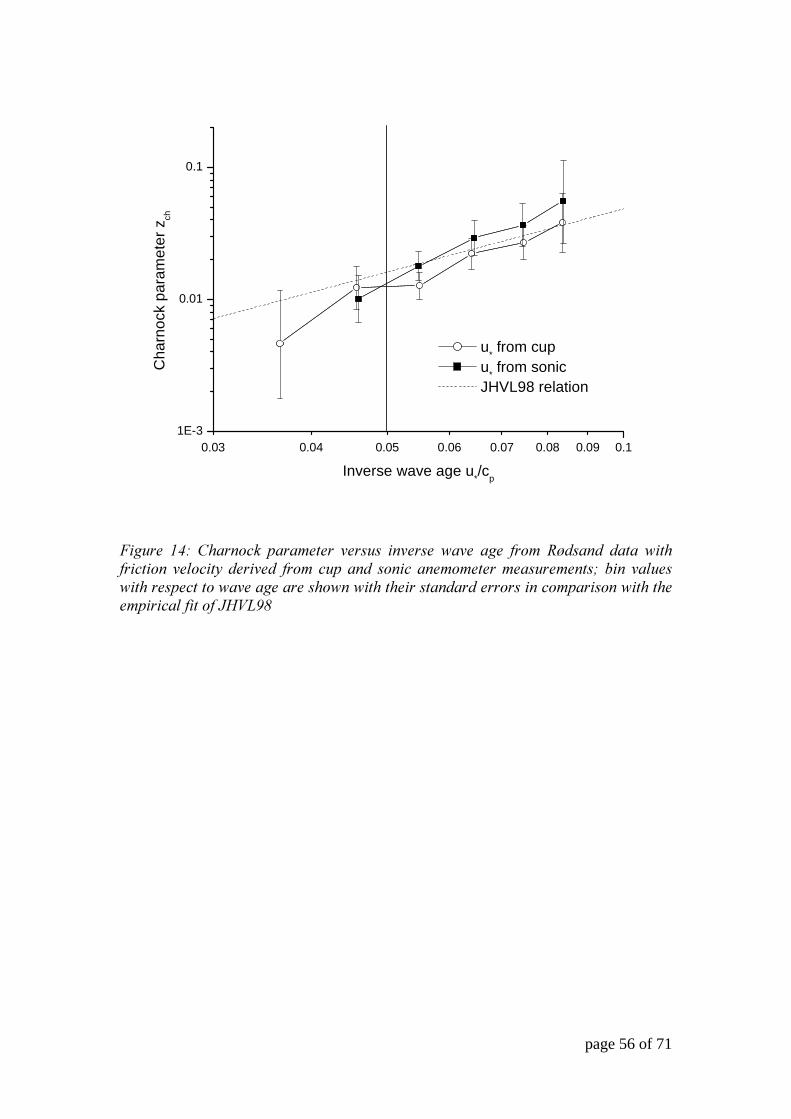
page 56 of 71

0.03 0.04 0.05 0.06 0.07 0.08 0.09 0.11E-3

0.01

0.1

u* from cup

u* from sonic

JHVL98 relation

Cha

rnoc

k pa

ram

eter

zch

Inverse wave age u*/c

p

2#���� 495 �(��!��� *�������� ������ #!����� ���� ��� ���� �1+��!+ +��� �#�(��#��#�! ��%��#�� +��#��+ ���� ��* �!+ ��!#� �!�����������������!��? �#! ��%����#�(���*����������������(��!�#�(�(�#����!+��+������#!���*��#��!�#�(�(���*#�#��%�#�����$&C

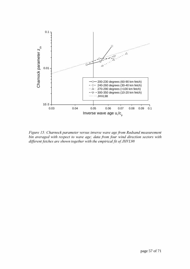
page 57 of 71

0.03 0.04 0.05 0.06 0.07 0.08 0.09 0.11E-3

0.01

0.1

Cha

rnoc

k pa

ram

eter

zch

Inverse wave age u*/c

p

200-230 degrees (60-90 km fetch) 240-260 degrees (30-40 km fetch) 270-290 degrees (>100 km fetch) 300-350 degrees (10-20 km fetch) JHVL98

2#����475�(��!���*��������������#!�����������������1+��!+���������!��#! �������+�#�( ���*��� ������ ���? +��� ���� �����#!+ +#����#�! ��������#�(+#�����!�����(������(��!�����(���#�(�(���*#�#��%�#�����$&C

page 58 of 71

0.1

0.01

0.1

Rødsand

Atlantic Ocean(short fetch)

Atlantic Ocean(long fetch)

HEXOS

RASEX

Lake Ontario

Cha

rnoc

k pa

ram

eter

zch

Inverse wave age u*/c

p

2#����4:5�������*%�����������+�(��!���*��������������#!���������������������%+��������!+���*��#��!�#�(�(���*#�#��%�#�����$&C

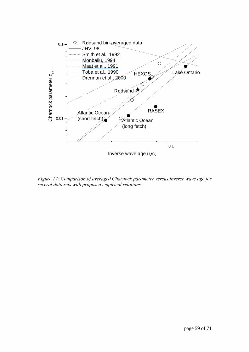
page 59 of 71

0.1

0.01

0.1 Rødsand bin-averaged data JHVL98 Smith et al., 1992 Monbaliu, 1994 Maat et al., 1991 Toba et al., 1990 Drennan et al., 2000

Rødsand

Atlantic Ocean(short fetch) Atlantic Ocean

(long fetch)

HEXOS

RASEX

Lake Ontario

Cha

rnoc

k pa

ram

eter

zch

Inverse wave age u*/c

p

2#����4B5���*��#��!���������+�(��!���*��������������#!���������������������%+��������#�(*��*���+��*#�#��%��%��#�!�

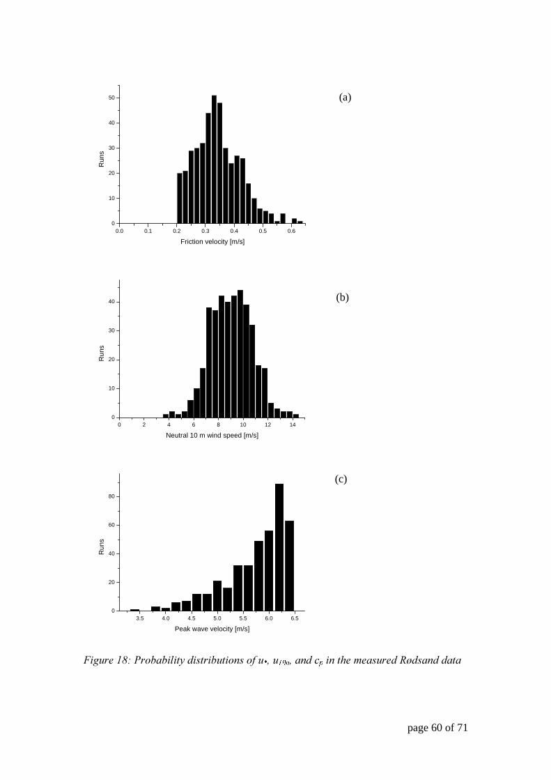
page 60 of 71

0.0 0.1 0.2 0.3 0.4 0.5 0.60

10

20

30

40

50R

uns

Friction velocity [m/s]

0 2 4 6 8 10 12 140

10

20

30

40

Run

s

Neutral 10 m wind speed [m/s]

3.5 4.0 4.5 5.0 5.5 6.0 6.50

20

40

60

80

Run

s

Peak wave velocity [m/s]

2#����4C5'�����#%#��+#���#���#�!���� -���Q-�!+�S#!�(��������+�1+��!++���

(a)

(b)

(c)

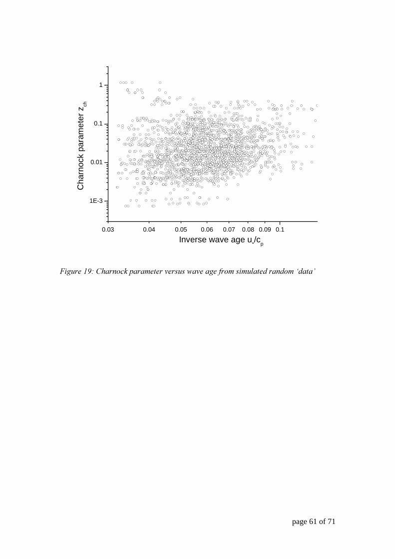
page 61 of 71

0.03 0.04 0.05 0.06 0.07 0.08 0.09 0.1

1E-3

0.01

0.1

1C

harn

ock

para

met

er z

ch

Inverse wave age u*/c

p

2#����4&5�(��!���*��������������������������#��%���+��!+��E+���F

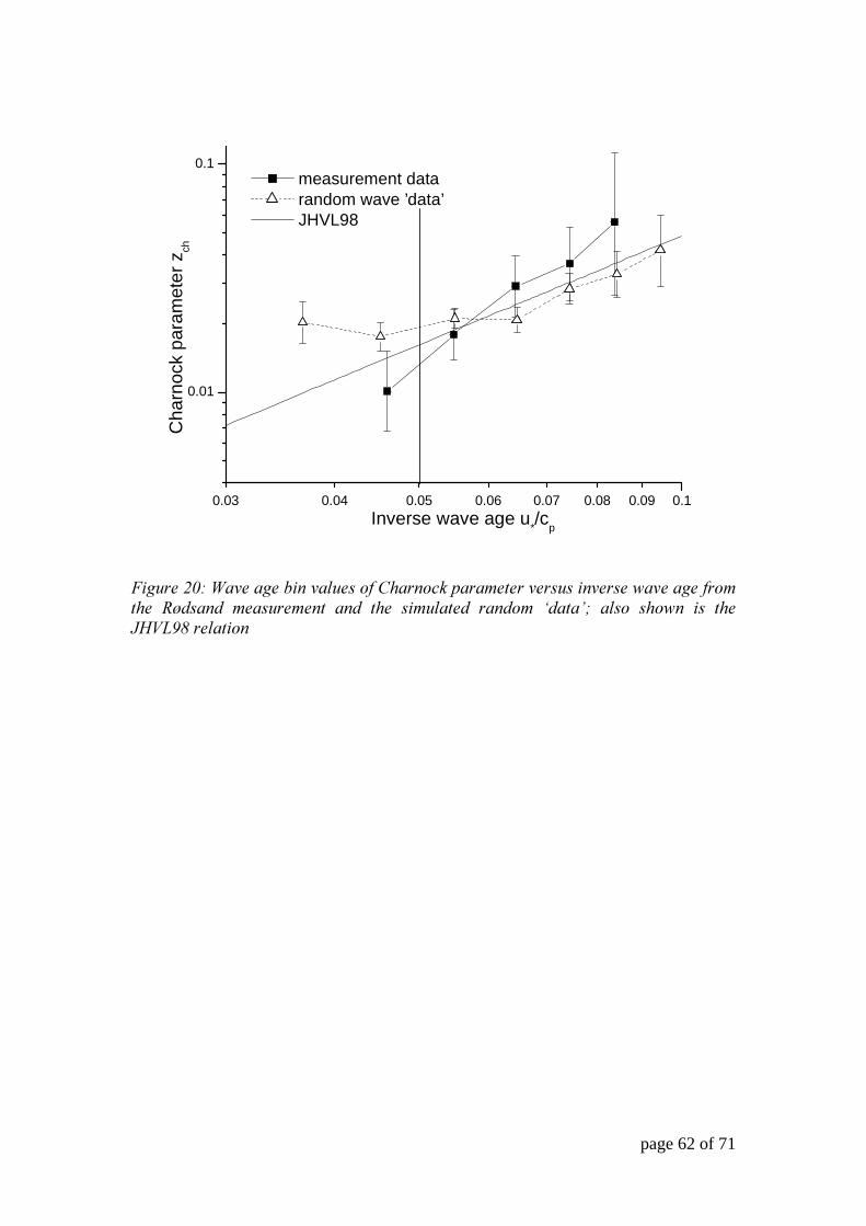
page 62 of 71

0.03 0.04 0.05 0.06 0.07 0.08 0.09 0.1

0.01

0.1 measurement data random wave ’data’ JHVL98

Cha

rnoc

k pa

ram

eter

zch

Inverse wave age u*/c

p

2#����685.�������#!��%������(��!���*��������������#!�����������������(� �1+��!+ ���������!� �!+ �(� �#��%���+ ��!+�� E+���F? �%�� �(��! #� �(���$&C��%��#�!

page 63 of 71

0.03 0.04 0.05 0.06 0.07 0.08 0.09 0.1

0.01

0.1 all measurement data all random wave ’data’ measurement data, c

p=6±0.2 m/s

random wave 'data', cp=6±0.2 m/s

Cha

rnoc

k pa

ram

eter

zch

Inverse wave age u*/c

p

2#����645���*��#��!���������+�*�!+�!�����(��!���*������������%%+����!+�+����������#�(����*(����*��+�S��:G8�6�>�?�(��!�������%�������(��1+��!+���������!��!+�#��%���+��!+��E+���F����

page 64 of 71

0.03 0.04 0.05 0.06 0.07 0.08 0.09 0.1

1E-3

0.01

0.1

1

data bin values direct fit fit to log

10(z

ch)

fit to bin values

Cha

rnoc

k pa

ram

eter

zch

Inverse wave age u*/c

p

2#���� 665 ���*��#��! �� ���(�+� �� �#� � *���� %�� ��%��#�! ������! �(��!���*���������!+#!���������������������++���

page 65 of 71

0.03 0.04 0.05 0.06 0.07 0.08 0.09 0.11E-3

0.01

0.1

inverse w.a. bins wind speed bins

10-12m/s8-10m/s

6-8m/s

Cha

rnoc

k pa

ram

eter

zch

Inverse wave age u*/c

p

2#���� 6<5 �(��!��� *�������� ������ ���� ��� ���� �1+��!+���������!�? �#!��%��������#!������#!��#�(���*�����#!������������;%������#�!�%��=�!+�#�(���*�����!�����%�#!+�*��+��48�(�#�(�;%�����A�����=����(��!����%%���#!��%�������� �(�+������������+�!+�#!�������+���( #!�#!+�*��+�!+ #!�������������#!�;���%%�A�����=

page 66 of 71

0.03 0.04 0.05 0.06 0.07 0.08 0.09 0.11E-3

0.01

0.1

1

Cha

rnoc

k pa

ram

eter

zch

Inverse wave age u*/c

p

5 km fetch 30 km fetch 100 km fetch 500 km fetch

2#����695��!�#�#�#�����(�����(!����%����#���#�!����$&C�#�(����(�!�*%�����(��!���*��������������#!������������;�FUH6�<=?����+�!�A���#�!6<

page 67 of 71

0.03 0.04 0.05 0.06 0.07 0.08 0.09 0.1

1E-3

0.01

0.1

1

Rcr=0.1

Rcr=0.5

Rcr=2.3

JHVL98 trend

Cha

rnoc

k pa

ram

eter

zch

Inverse wave age u*/c

p

no selection flow roughness > 0.1 flow roughness > 0.5 flow roughness > 2.3

2#���� 675 �(��!��� *�������� ������ #!����� ���� ��� ���� �1+��!+ +������������+�����+#!����%������(!���?�%���(��!����(�%#�#�#!�%#!�����A���#�!6<����!������#������(��<8���!+��FU��6�<-8�7�!+8�4

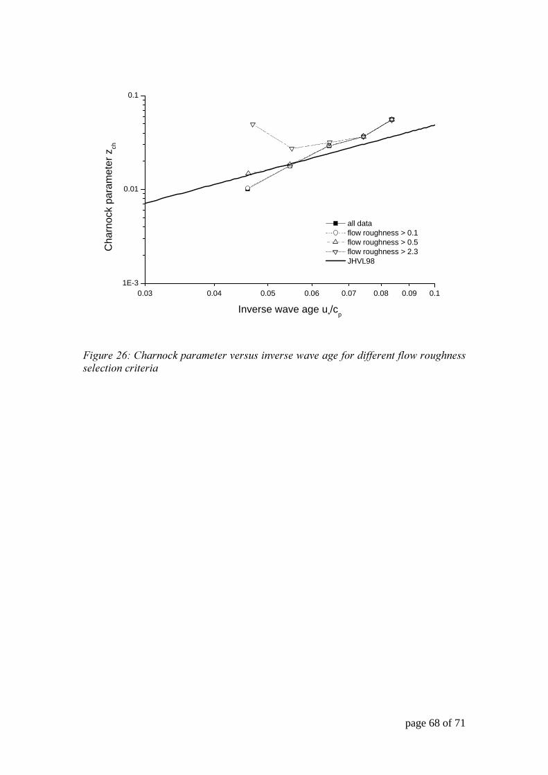
page 68 of 71

0.03 0.04 0.05 0.06 0.07 0.08 0.09 0.11E-3

0.01

0.1

all data flow roughness > 0.1 flow roughness > 0.5 flow roughness > 2.3 JHVL98

Cha

rnoc

k pa

ram

eter

zch

Inverse wave age u*/c

p

2#����6:5�(��!���*��������������#!���������������+#�����!��%������(!�����%���#�!��#���#�

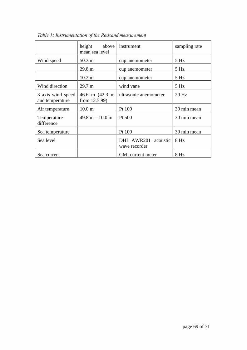
page 69 of 71

��%�4��3!������!���#�!���(��1+��!+���������!�

height above mean sea level

instrument sampling rate

Wind speed 50.3 m cup anemometer 5 Hz

29.8 m cup anemometer 5 Hz

10.2 m cup anemometer 5 Hz

Wind direction 29.7 m wind vane 5 Hz

3 axis wind speed and temperature

46.6 m (42.3 m from 12.5.99)

ultrasonic anemometer 20 Hz

Air temperature 10.0 m Pt 100 30 min mean

Temperature difference

49.8 m – 10.0 m Pt 500 30 min mean

Sea temperature Pt 100 30 min mean

Sea level DHI AWR201 acoustic wave recorder

8 Hz

Sea current GMI current meter 8 Hz

page 70 of 71

��%�65��%����+�#!++#����#�!��������#�(�**��/#����%��!#��������(

Direction [°] Name Fetch [km] number of records

200-230 Lübecker Bucht 60-90 102

240-260 Fehmarn 30-40 49

270-290 Femerbelt >100 77

300-350 Lolland 10-20 50

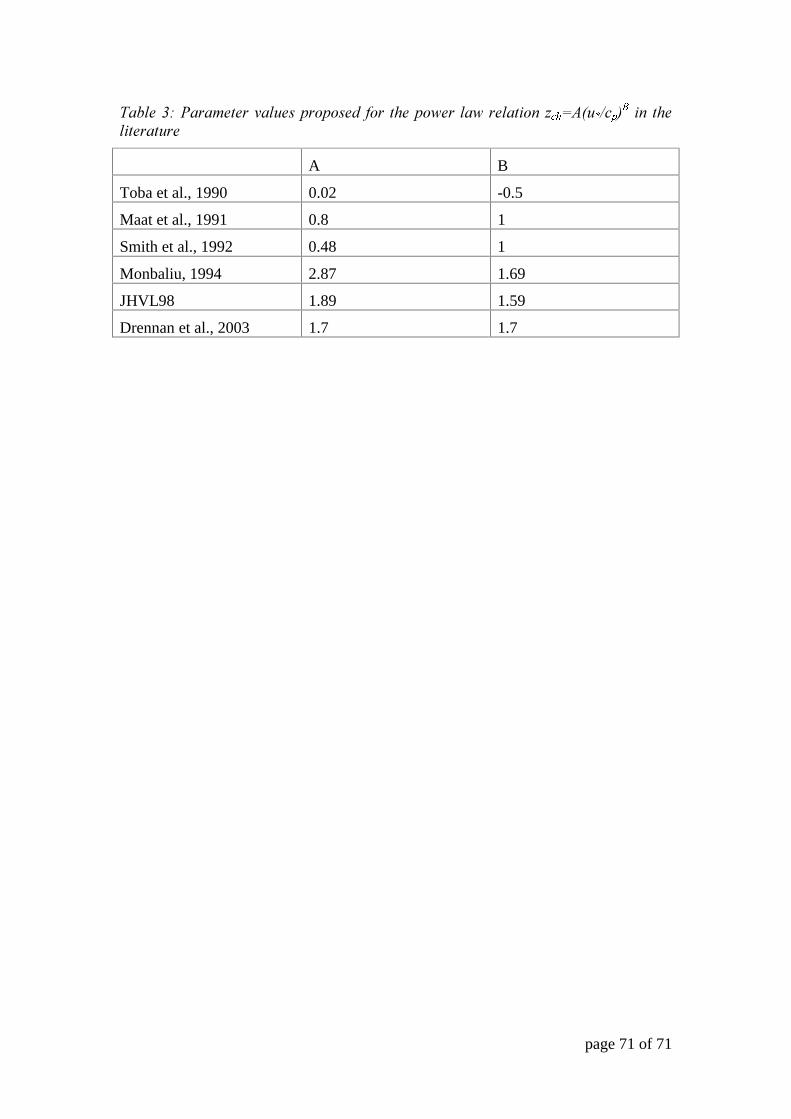
page 71 of 71

��%�<5'����������%���*��*���+ ��� �(�*���� %����%��#�!�FKH�;� >�S=% #! �(�

%#��������

A B

Toba et al., 1990 0.02 -0.5

Maat et al., 1991 0.8 1

Smith et al., 1992 0.48 1

Monbaliu, 1994 2.87 1.69

JHVL98 1.89 1.59

Drennan et al., 2003 1.7 1.7