


Bahasa
Halaman
Hukum


Nonlinear mechanics of rods, sheets and ribbons –interplay between geometry and mechanics
Gert van der Heijden
Department of Civil, Environmental & Geomatic EngineeringUniversity College London
Gert van der Heijden (UCL) Nonlinear mechanics of rods, sheets and ribbons 1 / 72

Outline
Nonlinear dynamics of large-deformation structures
Geometrically-exact theory of highly-flexible slender structures
We require:
Geometry of curves and surfacesCalculus of variationsNonlinear dynamics – bifurcation theory
We consider:
RodsRectangular strips/sheetsHelical ribbonsAnnular stripsMulti-strand structures (braids)
Quasi-rod theory
(joint work with Eugene Starostin)
Gert van der Heijden (UCL) Nonlinear mechanics of rods, sheets and ribbons 2 / 72

Examples of large deformations of 1D and 2Dstructures
(The need for nonlinear mechanics)
Gert van der Heijden (UCL) Nonlinear mechanics of rods, sheets and ribbons 3 / 72

Pipelines and cables
Marine pipelines: (a) (b)
( ) (d)
(e) (f)
Cables hanging under gravity (catenary)
Looping and loop pop-out of cables and pipelines (with self-contact)
Gert van der Heijden (UCL) Nonlinear mechanics of rods, sheets and ribbons 4 / 72

Mechanical modelling of DNA supercoiling
Single-molecule DNA experiments and (closed) DNA plasmids:
Gert van der Heijden (UCL) Nonlinear mechanics of rods, sheets and ribbons 5 / 72

Textile spinning
Whirling and snarling of a moving threadline (textile yarn ballooning):
Gert van der Heijden (UCL) Nonlinear mechanics of rods, sheets and ribbons 6 / 72

Magnetic buckling and space tethers
Magnetic buckling and electrodynamic space tethers (use earth’s magnetic fieldfor propulsion):
Post-buckling tether shapes (first and fifth mode):
z
y
x
z
y
x
Control of periodic orbits of a tether moving around the earthGert van der Heijden (UCL) Nonlinear mechanics of rods, sheets and ribbons 7 / 72

Hairstyle modelling
(Bertails et al., Eurographics, 2005)
Important effects of eccentricity, natural curliness and collisions, as well as wetting
Gert van der Heijden (UCL) Nonlinear mechanics of rods, sheets and ribbons 8 / 72

Animal and robotic whiskers
(Towal et al., PLoS Comput. Biol., 2011) (Solomon, Hartmann, Nature, 2006)
Gert van der Heijden (UCL) Nonlinear mechanics of rods, sheets and ribbons 9 / 72

Electrospinning
(Reneker & Yarin, Polymer, 2008)
Gert van der Heijden (UCL) Nonlinear mechanics of rods, sheets and ribbons 10 / 72

Other examples of slender one-dimensional structures
Viscous fluid jet (corn syrup) – bacterium (bacillus subtilis) – tendril (Darwin)
Gert van der Heijden (UCL) Nonlinear mechanics of rods, sheets and ribbons 11 / 72

Wrinkling and crumpling of sheets
Ripples in a stretched sheet – triangular buckling pattern in a twisted strip:
Gert van der Heijden (UCL) Nonlinear mechanics of rods, sheets and ribbons 12 / 72

Helical ribbons
Bistability of cholesterol ribbons:
Zastavker et al. (1999) Smith et al. (2001)
Zinc oxide and other nanosprings (Wang, 2007; Zhang et al., 2007):
Potential use in nanoscale force probes, transducersGert van der Heijden (UCL) Nonlinear mechanics of rods, sheets and ribbons 13 / 72

Annular nanostructures
Saddling of annular nanostructures:
(from: Cho et al., Nanoletters 10, 2010)
Gert van der Heijden (UCL) Nonlinear mechanics of rods, sheets and ribbons 14 / 72
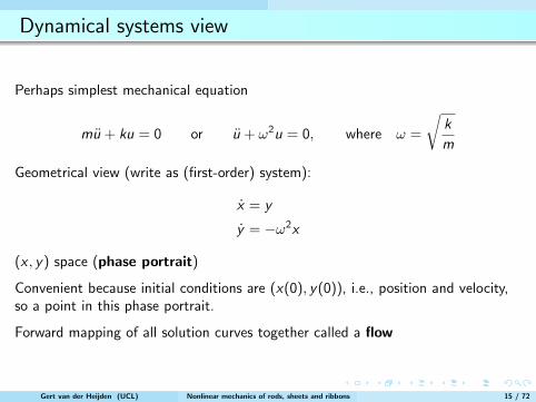
Dynamical systems view
Perhaps simplest mechanical equation
mu + ku = 0 or u + ω2u = 0, where ω =
√k
m
Geometrical view (write as (first-order) system):
x = y
y = −ω2x
(x , y) space (phase portrait)
Convenient because initial conditions are (x(0), y(0)), i.e., position and velocity,so a point in this phase portrait.
Forward mapping of all solution curves together called a flow
Gert van der Heijden (UCL) Nonlinear mechanics of rods, sheets and ribbons 15 / 72

Phase portrait
Phase portraits of x = f (x) with f = −U ′Gert van der Heijden (UCL) Nonlinear mechanics of rods, sheets and ribbons 16 / 72

Phase portrait of the pendulum
T =1
2ml2φ2
U = mg(l − l cosφ) = −mgl cosφ+ const.
Lagrangian: L = T − U
φ+ λ sinφ = 0, λ =g
lGert van der Heijden (UCL) Nonlinear mechanics of rods, sheets and ribbons 17 / 72

Phase portrait of the pendulum with damping
Gert van der Heijden (UCL) Nonlinear mechanics of rods, sheets and ribbons 18 / 72

Linearisation – fixed point stability
2D: u = Au, u = (x , y)T
Gert van der Heijden (UCL) Nonlinear mechanics of rods, sheets and ribbons 19 / 72

Change of stability in parametrised equations – bifurcations
Critical changes in the system’s behaviour as parameters are varied (change ofstability)
Possibilities (elementary bifurcations of 1D equilibria):
1) saddle-node or fold x = µ− x2
2) transcritical bifurcation x = µx − x2
Gert van der Heijden (UCL) Nonlinear mechanics of rods, sheets and ribbons 20 / 72

Bifurcations (cont’d)
3) pitchfork bifurcation x = µx − x3
4) Hopf bifurcation (involves a periodic solution, requires 2D)
Gert van der Heijden (UCL) Nonlinear mechanics of rods, sheets and ribbons 21 / 72

Pitchfork bifurcation theorem
A parametrised ODE
z = f (x , µ), (x , µ) ∈ R× R
with f satisfying f (−x , µ) = −f (x , µ) (hence x = 0 is a fixed point) and
∂f
∂x(0, µ0) = 0,
∂2f
∂x2(0, µ0) = 0,
∂3f
∂x3(0, µ0) 6= 0,
∂f
∂µ(0, µ0) = 0,
∂2f
∂x∂µ(0, µ0) 6= 0
has a pitchfork bifurcation at (x , µ) = (0, µ0).
x = µx − x3 x = µx + x3
(supercritical) (subcritical)Gert van der Heijden (UCL) Nonlinear mechanics of rods, sheets and ribbons 22 / 72

In second-order system
x = f (x) = −dV
dx
saddle-node:
x + x2 − µ = 0
(V (x) =
1
3x3 − µx
)[
x = yy = µ− x2 linearisation: z = Az , A =
(0 1−2x 0
)Fixed points: y = 0, x = ±√µ (µ ≥ 0)
Eigenvalues: λ2 + 2x = 0
x =√µ: λ1,2 = ±i
√2√µ (centre)
x = −√µ: λ1,2 = ±√
2õ (saddle)
Gert van der Heijden (UCL) Nonlinear mechanics of rods, sheets and ribbons 23 / 72

pitchfork bifurcation:
x + x3 − µx = 0
(V (x) =
1
4x4 − 1
2µx2
)[
x = yy = µx − x3 linearisation: z = Az , A =
(0 1
µ− 3x2 0
)Fixed points: y = 0, x = 0, ±√µ
Eigenvalues: λ2 − (µ− 3x2) = 0
x = 0: λ1,2 = ±√µ (centre for µ < 0, saddle for µ > 0)
x = ±√µ: λ1,2 = ±i√
2µ (µ > 0) (centre)
x = µx − x3 x = µx + x3
(supercritical) (subcritical)
Gert van der Heijden (UCL) Nonlinear mechanics of rods, sheets and ribbons 24 / 72

2D elastic rod – Euler elastica
Euler elastica
x ′ = cos θ, y ′ = sin θ
Elastic energy: U = 12B
∫ S
0
κ2 ds, curvature κ = θ′, M = Bκ, B = EI
Work done by end load: W = −PD = −P∫ S
0
(1− cos θ)ds
Total potential energy: V = U + W =
∫ S
0
L(θ, θ′)ds, L = 12Bθ
′2 + P cos θ
Energy minimisation: Bθ′′ + P sin θ = 0 (equilibrium equation)
Static-dynamic analogy
Gert van der Heijden (UCL) Nonlinear mechanics of rods, sheets and ribbons 25 / 72

Euler elastica (phase portrait and elastic shapes)
Centreline equations: x ′ = cos θ, y ′ = sin θ
Gert van der Heijden (UCL) Nonlinear mechanics of rods, sheets and ribbons 26 / 72

The elastica
Gert van der Heijden (UCL) Nonlinear mechanics of rods, sheets and ribbons 27 / 72

(Spatial) chaos
(1) Intrinsic curvature:
M = EI (κ− κ0), κ =dθ
dsFor instance, sinusoidal nonstraightness: κ0 = κ sinωs
EId2θ
ds2+ F sin θ = EI
dκ0
ds= EI κω cosωs =: α cosωs
(periodic forcing)
(2) Varying cross-section: EI = EI (s)
For instance, sinusoidally varying stiffness: EI = B0 + B1 sinωs
B0d2θ
ds2+ F sin θ = −ωB1 cosωs
dθ
ds− B1 sinωs
d2θ
ds2
(parametric forcing)
Gert van der Heijden (UCL) Nonlinear mechanics of rods, sheets and ribbons 28 / 72

IVP vs. BVP
θ′′ + α2 sin θ = 0 (α2 = P/EI or g/L)
IVP: θ(0) = θ0, θ′(0) = 0
BVP: θ′(0) = 0 = θ′(L) (pinned-pinned boundary conditions)
α1 α2 α3
Length constraint: L =
∫ds =
∫ −θ0
θ0
dθ
θ′(integral: 1
2θ′2 − α2 cos θ = h)
Gert van der Heijden (UCL) Nonlinear mechanics of rods, sheets and ribbons 29 / 72

Stability analysis for the pendulum – spectral stability
θ′′ + α2 sin θ = 0 (α2 = g/L)
Written as a dynamical system (x = θ, y = θ′):[x ′ = yy ′ = −α sin x
Jacobian at downward hanging equilibrium (x , y) = (0, 0):
J =
(0 1
−α cos x 0
)=
(0 1−α 0
)Eigenvalues: λ2 + α = 0 =⇒ λ = ±i
√α
i.e., (stable) centre point for all α
Gert van der Heijden (UCL) Nonlinear mechanics of rods, sheets and ribbons 30 / 72

Solving a boundary-value problem – buckling
Column of length L with pinned ends under a compressive load P
Loss of stability of the straight solution – buckling
Need only consider linearised equation about θ = 0:
θ′′ + λθ = 0
(λ =
P
EI
), θ′(0) = 0, θ′(L) = 0
Solution: θ(s) = A sin√λs + B cos
√λs
Critical loads: λ =n2π2
L2(n = 1, 2, ...)
Gert van der Heijden (UCL) Nonlinear mechanics of rods, sheets and ribbons 31 / 72
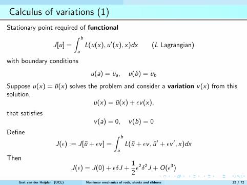
Calculus of variations (1)
Stationary point required of functional
J[u] =
∫ b
a
L(u(x), u′(x), x)dx (L Lagrangian)
with boundary conditions
u(a) = ua, u(b) = ub
Suppose u(x) = u(x) solves the problem and consider a variation v(x) from thissolution,
u(x) = u(x) + εv(x),
that satisfiesv(a) = 0, v(b) = 0
Define
J(ε) := J[u + εv ] =
∫ b
a
L(u + εv , u′ + εv ′, x)dx
Then
J(ε) = J(0) + εδJ +1
2ε2δ2J + O(ε3)
Gert van der Heijden (UCL) Nonlinear mechanics of rods, sheets and ribbons 32 / 72

Calculus of variations (2)
δJ =dJ(ε)
dε
∣∣∣∣ε=0
=
∫ b
a
[Lu(u, u′, x)v + Lu′(u, u′, x)v ′]dx (first variation)
δ2J =d2J(ε)
dε2
∣∣∣∣ε=0
=
∫ b
a
[Luu(u, u′, x)v2+2Luu′(u, u′, x)vv ′+Lu′u′(u, u′, x)(v ′)2]dx
(second variation)
For a local minimum:
Stationarity:
δJ =
∫ b
a
(Lu −
d
dxLu′
)v dx = 0 (for all variations v)
=⇒ d
dx
(∂L
∂u′
)− ∂L
∂u= 0 (Euler-Lagrange equation)
Minimum ifδ2J > 0 (for all variations v 6= 0)
Gert van der Heijden (UCL) Nonlinear mechanics of rods, sheets and ribbons 33 / 72
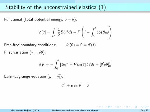
Stability of the unconstrained elastica (1)
Functional (total potential energy, u = θ):
V [θ] =
∫ l
0
1
2Bθ′2ds − P
(l −∫ l
0
cos θds
)
Free-free boundary conditions: θ′(0) = 0 = θ′(l)
First variation (v = δθ):
δV = −∫ l
0
[Bθ′′ + P sin θ] δθds + [θ′δθ]l0
Euler-Lagrange equation (p = PB ):
θ′′ + p sin θ = 0
Gert van der Heijden (UCL) Nonlinear mechanics of rods, sheets and ribbons 34 / 72

Stability of the unconstrained elastica (2)
Second variation:
δ2V =
∫ l
0
[(δθ′)2 − (δθ)2p cos θ
]ds
or, after integration by parts,
δ2V = −∫ l
0
[δθ′′ + δθp cos θ] δθds
Consider the Sturm-Liouville problem (linearised Euler-Lagrange equation):
φ′′ + µp cos θφ = 0, φ′(0) = 0 = φ′(l)
This has real eigenvalues µn and a basis of eigenfunctions φn (n = 1, 2, ...)satisfying the orthogonality condition∫ l
0
φn(s)φm(s)p cos θ(s)ds = 0 (n 6= m)
Gert van der Heijden (UCL) Nonlinear mechanics of rods, sheets and ribbons 35 / 72

Stability of the unconstrained elastica (3)
Thus we can write
δθ(s) =∞∑n=1
cnφn(s)
and
δ2V =
∫ l
0
∞∑n=1
(µn − 1)p cos θc2nφ
2nds
or, using the identity µn
∫ l
0
p cos θ(s)φ2nds =
∫ l
0
(φ′n(s))2ds,
δ2V =∞∑n=1
(1− 1
µn
)c2n
∫ l
0
(φ′n(s))2ds
So we havestability if µn /∈ [0, 1]
instability if µn ∈ [0, 1]
(for all n)
Gert van der Heijden (UCL) Nonlinear mechanics of rods, sheets and ribbons 36 / 72

Stability of the unconstrained elastica (4)
Stability of the straight solution (θ = 0):
Sturm-Liouville problem:
φ′′ + µpφ = 0, φ′(0) = 0 = φ′(l)
Nontrivial solutions (eigenfunctions):
φn(s) = cosnπs
l, µn =
n2π2
pl2=
Pcrn
P, Pcr
n =n2π2B
l2
Conclusion:
The straight configuration is stable for P < Pcr0 = 0 and unstable for P > 0
(µ = 0 is an eigenvalue with corresponding rigid-body rotation mode φ = const.)
The solution θ = const. for P = 0 is marginally stable
Rigid-body mode (constant variation) δθ = a (θ = 0):
δ2V = −∫ l
0[δθ′′ + p cos θδθ] δθds = −
∫ l
0pa2ds = −pla2 < 0
Indeed, taking θ = θ0: V (θ0) =∫ l
0( 1
2θ′20 + p cos θ0)ds = pl cos θ0 < pl = V (0)
Gert van der Heijden (UCL) Nonlinear mechanics of rods, sheets and ribbons 37 / 72

Stability of the constrained elastica – pinned (1)
Functional (total potential energy + constraint, λ Lagrange multiplier):
V [θ] =
∫ l
0
1
2Bθ′2ds − P
(l −∫ l
0
cos θds
)− λ
∫ l
0
sin θds
Pinned-pinned boundary conditions: θ′(0) = 0 = θ′(l), ∆y =
∫ l
0
sin θds = 0
First variation:
δV = −∫ l
0
[Bθ′′ + P sin θ + λ cos θ] δθds + [θ′δθ]l0
Euler-Lagrange equation (p = PB , λ = λ
B ): θ′′ + p sin θ + λ cos θ = 0
Integrate: λ = 0 (no shear force, unless ends coincide)
Constraint: C [θ] =
∫ l
0
sin θds = 0
So variations δθ satisfy the linearised constraint
δC =
∫ l
0
δθ cos θds = 0
Gert van der Heijden (UCL) Nonlinear mechanics of rods, sheets and ribbons 38 / 72

Stability of the constrained elastica – pinned (2)
Second variation (noting λ = 0):
δ2V =
∫ l
0
[(δθ′)2 − (δθ)2p cos θ
]ds
or, after integration by parts,
δ2V = −∫ l
0
[δθ′′ + pδθ cos θ] δθds
Consider the (inhomogeneous) Sturm-Liouville problem (linearised Euler-Lagrangeequation, c free parameter):
φ′′ + µp cos θφ = c cos θ, φ′(0) = 0 = φ′(l)
subject to
∫ l
0
φ cos θds = 0
Integrate: c = 0 (no (linearised) shear force, unless ends coincide)
This has real eigenvalues µn and a basis of eigenfunctions φn (n = 1, 2, ...) with∫ l
0
φn(s)φm(s)p cos θ(s)ds = 0 (n 6= m)
Gert van der Heijden (UCL) Nonlinear mechanics of rods, sheets and ribbons 39 / 72

Stability of the constrained elastica – pinned (3)
Thus we can write
δθ(s) =∞∑n=1
cnφn(s)
and
δ2V =
∫ l
0
∞∑n=1
(µn − 1)p cos θc2nφ
2nds
or, using the identity µn
∫ l
0
p cos θ(s)φ2nds =
∫ l
0
(φ′n(s))2ds,
δ2V =∞∑n=1
(1− 1
µn
)c2n
∫ l
0
(φ′n(s))2ds
So we havestability if µn /∈ [0, 1]
instability if µn ∈ [0, 1]
(for all n)
Gert van der Heijden (UCL) Nonlinear mechanics of rods, sheets and ribbons 40 / 72

Stability of the constrained elastica – pinned (4)
Stability of the straight solution (θ = 0):
Sturm-Liouville problem (c = 0):
φ′′ + µpφ = 0, φ′(0) = 0 = φ′(l),
∫ l
0
φ ds = 0
Nontrivial solutions (eigenfunctions):
φn(s) = cosnπs
l, µn =
n2π2
pl2=
Pcrn
P, Pcr
n =n2π2B
l2
Conclusion:
The straight configuration is stable for P < Pcr1 and unstable for P > Pcr
1
(Rigid-body mode, and hence zero eigenvalue, eliminated by the constraint)
Gert van der Heijden (UCL) Nonlinear mechanics of rods, sheets and ribbons 41 / 72

Eigenvalues of the free-free elastica
1st mode 2nd mode
-2
0
2
4
6
8
10
-4 -3 -2 -1 0 1 2 3 4
µ
θ(L)
-2
0
2
4
6
8
10
-4 -3 -2 -1 0 1 2 3 4
µ
θ(L)
3rd mode
-2
0
2
4
6
8
10
-4 -3 -2 -1 0 1 2 3 4
µ
θ(L)
Coincident ends: K (k) = 2E (k), k = 0.9089, p = 21.5491 (θ(l) = 130.71◦)
Gert van der Heijden (UCL) Nonlinear mechanics of rods, sheets and ribbons 42 / 72

Eigenvalue continuation – solving an IVP
θ′′ + p sin θ = 0, θ′(0) = 0, θ′(l) = 0
φ′′ + µp cos θ φ = 0, φ′(0) = 0, φ′(l) = 0 (−→ φ(0) = 1)
First three (non-rigid-body) modes of the free-free rod:
-10
-5
0
5
10
0 0.5 1 1.5 2
φ’(
l)
µ
1st mode: p = 10.7064, 2nd mode: p = 41.3133, 3rd mode: p = 92.9550
Gert van der Heijden (UCL) Nonlinear mechanics of rods, sheets and ribbons 43 / 72

Pinned elastica – secondary instability
Gert van der Heijden (UCL) Nonlinear mechanics of rods, sheets and ribbons 44 / 72

Bifurcation diagrams for a twisted rod
varying end rotation(R = 0 (a), π (b), 2π (c),3π (d), 4π (e) and 8.9527
(f))(solid curves stable under
rigid loading) zero end rotation (R = 0), varying Poisson’s ratio(γ = C
B = 1.7, 1.8, 3.2, 12.0)
Gert van der Heijden (UCL) Nonlinear mechanics of rods, sheets and ribbons 45 / 72
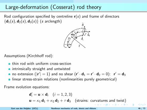
Large-deformation (Cosserat) rod theory
Rod configuration specified by centreline r(s) and frame of directors{d1(s),d2(s),d3(s)} (s arclength)
Assumptions (Kirchhoff rod):
thin rod with uniform cross-section
intrinsically straight and untwisted
no extension (|r′| = 1) and no shear (r′ · d1 = r′ · d2 = 0): r′ = d3
linear stress-strain relations (nonlinearities purely geometrical)
Frame evolution equations:
d′i = u× di (i = 1, 2, 3)
u = κ1 d1 + κ2 d2 + τ d3 (strains: curvatures and twist)
Gert van der Heijden (UCL) Nonlinear mechanics of rods, sheets and ribbons 46 / 72

Kinematics - frame evolution equation
Orthonormality:d i · d i = 1 =⇒ d
′i · d i = 0
d i · d j = 0 =⇒ d′i · d j = −d ′j · d i
Thus we can write (for some functions κ1, κ2, τ):
d′1 = τd 2 − κ2d 3
d′2 = −τd 1 + κ1d 3
d′3 = κ2d 1 − κ1d 2
ord′i = u × d i (i = 1, 2, 3),
whereu = κ1d 1 + κ2d 2 + τd 3 (strain vector)
κ1 and κ2 are the curvatures (about d 1 and d 2) and τ is the twist (about d 3)
Note the analogy with angular velocity in rigid-body dynamics!
Gert van der Heijden (UCL) Nonlinear mechanics of rods, sheets and ribbons 47 / 72

Force and moment balance
Force balance:
F (s + ∆s)− F (s) +
∫ s+∆s
s
f (s) ds = 0
⇐⇒∫ s+∆s
s
F′(s)ds +
∫ s+∆s
s
f (s) ds
=
∫ s+∆s
s
[F ′(s) + f (s)] ds = 0
ThusF′ + f = 0
Moment balance:
M(s + ∆s)−M(s) + r(s + ∆s)× F (s + ∆s)− r(s)× F (s) +
∫ s+∆s
s
r × f ds = 0
⇐⇒∫ s+∆s
s
[M ′ + (r × F )′ + r × f ] ds = 0
Thus M′ + r ′ × F = 0
Gert van der Heijden (UCL) Nonlinear mechanics of rods, sheets and ribbons 48 / 72

3D deformation – elastic (Cosserat) rod equations
−60−40
−200
−40−20
020
−300
−250
−200
−150
−100
−50
0
Equilibrium equations (F force, M moment): F′ = 0, M
′ + r ′ × F = 0
Frame evolution equation: d′i = u × d i (i=1,2,3)
Inextensible rod: r ′ = d 3 (unit tangent)
Expressed in the moving (body) frame {d 1,d 2,d 3} (F = (F1,F2,F3), Fi = F ·d i ):
F′ + u× F = 0, M′ + u×M + d3 × F = 0, d3 = (0, 0, 1)
u = (κ1, κ2, τ) (strains; κ1, κ2 curvatures, τ twist)
Linear elasticity (Hooke’s law): M1 = B1κ1, M2 = B2κ2, M3 = Cτ
B1, B2 bending stiffnesses, C torsional stiffnessGert van der Heijden (UCL) Nonlinear mechanics of rods, sheets and ribbons 49 / 72

Dynamic analogy – spinning top
Equations of motion (L angular momentum, v vector from fixed point to centre ofmass): L
′ = mgk × v (torque due to gravity, k vertical)
Expressed relative to the rotating (body) frame (principal axes), including k′ = 0:
k′ + ω × k = 0, L′ + ω × L + mgv × k = 0, v = (0, 0, l)
ω angular velocity (assume centre of mass lies on one of the principal axes)
L1 = I1ω1, L2 = I2ω2, L3 = I3ω3
I1, I2, I3 moments of inertia
Kirchhoff dynamic analogy
Gert van der Heijden (UCL) Nonlinear mechanics of rods, sheets and ribbons 50 / 72

Reduction of the equilibrium equations in the isotropic case
d′i = u × d i for i = 1, 2, 3
ui =1
2εijk d
′j · d k
κ1 = θ′ sinφ− ψ′ sin θ cosφ
κ2 = θ′ cosφ+ ψ′ sin θ sinφ
τ = φ′ + ψ′ cos θ
Choice of fixed frame:
F′ = 0 −→ F (s) = T e3
Lagrangian:
L =1
2B1κ
21 +
1
2B2κ
22 +
1
2Cτ 2 − T e3 · d 3 = L(θ, ψ, φ, θ′, ψ′, φ′)
Isotropic rod (symmetric cross-section): B1 = B2 = B
Gert van der Heijden (UCL) Nonlinear mechanics of rods, sheets and ribbons 51 / 72

Euler angles to parametrise the body frame
The body co-ordinate system {d 1,d 2,d 3} can be related to a fixed orthonormalsystem {e1, e2, e3} via the Euler angles θ, ψ, φ:
d 1 = (− sinψ sinφ+ cosψ cosφ cos θ) e1 +
(cosψ sinφ+ sinψ cosφ cos θ) e2 − cosφ sin θ e3,
d 2 = (− sinψ cosφ− cosψ sinφ cos θ) e1 +
(cosψ cosφ− sinψ sinφ cos θ) e2 + sinφ sin θ e3,
d 3 = cosψ sin θ e1 + sinψ sin θ e2 + cos θ e3.
Gert van der Heijden (UCL) Nonlinear mechanics of rods, sheets and ribbons 52 / 72

Conserved quantities:
d
ds(M · e3) = 0 (moment about force, ψ cyclic)
d
ds(M · d 3) = 0 (twisting moment, φ cyclic)
d
ds
(1
2B1κ
21 +
1
2B2κ
22 +
1
2Cτ 2 + T d 3 · e3
)= 0 (‘energy’)
(Linear) constitutive relations: M1 = B1κ1, M2 = B2κ2, M3 = Cτ
β = M · d 3 = M3 = Cτ
α = M · e3 =3∑
i=1
Mi d i · e3 = Bκ1 d 1 · e3 + Bκ2 d 2 · e3 + Cτ d 3 · e3
= −Bκ1 cosφ sin θ + Bκ2 sinφ sin θ + β cos θ
ψ′ =α− β cos θ
B sin2 θ, φ′ =
β
C− ψ′ cos θ
Gert van der Heijden (UCL) Nonlinear mechanics of rods, sheets and ribbons 53 / 72

Planar system (for isotropic rod or Lagrange top):
Bθ′′ +dV
dθ= 0, V (θ) =
(α− β cos θ)2
2B sin2 θ+ T cos θ
For a straight rod (or upright top) we need to take α = β = M0
(d 3 and e3 aligned, M0 applied twisting moment)
V (θ) =M2
2B
1− cos θ
1 + cos θ+ T cos θ
Dimensionless:
1
2θ′
2+ V (θ) = h, V (θ) =
1
2
1− cos θ
1 + cos θ+
cos θ
m2, m =
M0√BT
Special case: M0 = 0 −→ α = β = 0 −→ Euler elastica
Gert van der Heijden (UCL) Nonlinear mechanics of rods, sheets and ribbons 54 / 72

Buckling of an isotropic rod – falling over of Lagrange top
Reduced 1-DOF equation (θ is angle between tangent and F ):
θ′′ +dV (θ)
dθ= 0, V (θ) =
1
2
1− cos θ
1 + cos θ+
cos θ
m2
(m =
M0√BT
)(same as for Lagrange, i.e., symmetric, top)
Typical phase portraits:
m > 2 m < 2
Gert van der Heijden (UCL) Nonlinear mechanics of rods, sheets and ribbons 55 / 72
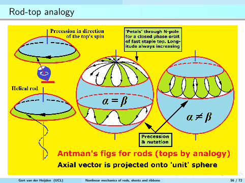
Rod-top analogy
Gert van der Heijden (UCL) Nonlinear mechanics of rods, sheets and ribbons 56 / 72

Localised buckling of isotropic rod
Fixed points: dV /dθ = 0 (nonzero θ: helical rod, precessing top)
Eigenvalues of trivial fixed point θ = 0: λ1,2 = ±(1/2m)√
4−m2
θ′′ = −dV
dθ=
− sin θ
(1 + cos θ)2+
sin θ
m2=
(1
m2− 1
4
)θ −
(1
12+
1
6m2
)θ3 + O
(θ5)
Supercritical pitchfork bifurcation at m = 2
Homoclinic orbit (localised solution):
cos θ(s) = u0 + (1− u0) tanh2
(√1− u0
m√
2s
), u0 =
1
2m2 − 1
z
y
0 15 30 45 60 75 90 105 120 135 150-1.0
-0.8
-0.6
-0.4
-0.2
0.0
0.2
0.4
0.6
0.8
1.0
Gert van der Heijden (UCL) Nonlinear mechanics of rods, sheets and ribbons 57 / 72

3D bifurcation diagram
Equivalent oscillator for the twisted circular rod:
Note inversion of stability!Gert van der Heijden (UCL) Nonlinear mechanics of rods, sheets and ribbons 58 / 72

Localised solutions
Shape obtained by integrating the centreline equation r ′ = d 3
z
x
0 15 30 45 60 75 90 105 120 135 150-0.5
-0.4
-0.3
-0.2
-0.1
0.0
0.1
0.2
0.3
0.4
0.5
z
y
0 15 30 45 60 75 90 105 120 135 150-0.5
-0.4
-0.3
-0.2
-0.1
0.0
0.1
0.2
0.3
0.4
0.5
z
x0 15 30 45 60 75 90 105 120 135 150
-1.0
-0.8
-0.6
-0.4
-0.2
0.0
0.2
0.4
0.6
0.8
1.0
z
y
0 15 30 45 60 75 90 105 120 135 150-1.0
-0.8
-0.6
-0.4
-0.2
0.0
0.2
0.4
0.6
0.8
1.0
z
x
0 15 30 45 60 75 90 105 120 135 150-1.80
-1.44
-1.08
-0.72
-0.36
0.00
0.36
0.72
1.08
1.44
1.80
z0 15 30 45 60 75 90 105 120 135 150
-1.80
-1.44
-1.08
-0.72
-0.36
0.00
0.36
0.72
1.08
1.44
1.80Gert van der Heijden (UCL) Nonlinear mechanics of rods, sheets and ribbons 59 / 72

Localised solutions (true 3D views)
Gert van der Heijden (UCL) Nonlinear mechanics of rods, sheets and ribbons 60 / 72
Top Related
Copyright © 2022 FDOKUMEN

