


Bahasa
Halaman
Hukum

Submitted to the Annals of Statistics
NEAR OPTIMAL SAMPLE COMPLEXITY FOR MATRIX AND TENSORNORMAL MODELS VIA GEODESIC CONVEXITY
BY COLE FRANKS1, RAFAEL OLIVEIRA2,*, AKSHAY RAMACHANDRAN2,†
AND MICHAEL WALTER3
1Department of Mathematics, Massachusetts Institute of Technology, [email protected]
2Cheriton School of Computer Science, University of Waterloo, *[email protected]; †[email protected]
3Korteweg-de Vries Institute for Mathematics and Institute for Theoretical Physics, University of Amsterdam, [email protected]
The matrix normal model, the family of Gaussian matrix-variate dis-tributions whose covariance matrix is the Kronecker product of two lowerdimensional factors, is frequently used to model matrix-variate data. Thetensor normal model generalizes this family to Kronecker products of threeor more factors. We study the estimation of the Kronecker factors of the co-variance matrix in the matrix and tensor models. We show nonasymptoticbounds for the error achieved by the maximum likelihood estimator (MLE) inseveral natural metrics. In contrast to existing bounds, our results do not relyon the factors being well-conditioned or sparse. For the matrix normal model,all our bounds are minimax optimal up to logarithmic factors, and for thetensor normal model our bound for the largest factor and overall covariancematrix are minimax optimal up to constant factors provided there are enoughsamples for any estimator to obtain constant Frobenius error. In the sameregimes as our sample complexity bounds, we show that an iterative procedureto compute the MLE known as the flip-flop algorithm converges linearly withhigh probability. Our main tool is geodesic strong convexity in the geometryon positive-definite matrices induced by the Fisher information metric. Thisstrong convexity is determined by the expansion of certain random quantumchannels. We also provide numerical evidence that combining the flip-flopalgorithm with a simple shrinkage estimator can improve performance in theundersampled regime.
CONTENTS
1 Introduction . . . . . . . . . . . . . . . . . . . . . . . . . . . . . . . . . . . . . . 21.1 Our contributions . . . . . . . . . . . . . . . . . . . . . . . . . . . . . . . . 41.2 Outline . . . . . . . . . . . . . . . . . . . . . . . . . . . . . . . . . . . . . 51.3 Notation . . . . . . . . . . . . . . . . . . . . . . . . . . . . . . . . . . . . . 6
2 Model and main results . . . . . . . . . . . . . . . . . . . . . . . . . . . . . . . . 62.1 Matrix and tensor normal model . . . . . . . . . . . . . . . . . . . . . . . . 62.2 Results on the MLE . . . . . . . . . . . . . . . . . . . . . . . . . . . . . . . 72.3 Flip-flop algorithm . . . . . . . . . . . . . . . . . . . . . . . . . . . . . . . 92.4 Results on the flip-flop algorithm . . . . . . . . . . . . . . . . . . . . . . . . 10
3 Sample complexity for the tensor normal model . . . . . . . . . . . . . . . . . . . 103.1 Geodesic convexity . . . . . . . . . . . . . . . . . . . . . . . . . . . . . . . 113.2 Sketch of proof . . . . . . . . . . . . . . . . . . . . . . . . . . . . . . . . . 123.3 Bounding the gradient . . . . . . . . . . . . . . . . . . . . . . . . . . . . . 153.4 Strong convexity from expansion . . . . . . . . . . . . . . . . . . . . . . . . 18
MSC2020 subject classifications: Primary 62F12; secondary 62F30.Keywords and phrases: Covariance estimation, matrix normal model, tensor normal model, maximum likeli-
hood estimation, geodesic convexity, operator scaling.
1
arX
iv:2
110.
0758
3v2
[m
ath.
ST]
11
Nov
202
1
2 C. FRANKS, R. OLIVEIRA, A. RAMACHANDRAN AND M. WALTER
3.5 Proof of Theorem 2.4 . . . . . . . . . . . . . . . . . . . . . . . . . . . . . . 234 Improvements for the matrix normal model . . . . . . . . . . . . . . . . . . . . . 25
4.1 Spectral gap and expansion . . . . . . . . . . . . . . . . . . . . . . . . . . . 254.2 Proof of Theorem 2.7 . . . . . . . . . . . . . . . . . . . . . . . . . . . . . . 27
5 Convergence of the flip-flop algorithm . . . . . . . . . . . . . . . . . . . . . . . . 305.1 Proofs of Theorem 2.9 and 2.10 . . . . . . . . . . . . . . . . . . . . . . . . 36
6 Lower bounds . . . . . . . . . . . . . . . . . . . . . . . . . . . . . . . . . . . . . 386.1 Lower bounds for unstructured precision matrices . . . . . . . . . . . . . . . 386.2 Lower bounds for the matrix normal model . . . . . . . . . . . . . . . . . . 40
7 Numerics and regularization . . . . . . . . . . . . . . . . . . . . . . . . . . . . . 427.1 ShrinkFlop estimator . . . . . . . . . . . . . . . . . . . . . . . . . . . . . . 437.2 Scenario 1: Spiked, dense covariances . . . . . . . . . . . . . . . . . . . . . 437.3 Scenario 2: Sparse and partially sparse precision matrices . . . . . . . . . . . 447.4 Performance as a function of the number of samples . . . . . . . . . . . . . 447.5 Computational aspects . . . . . . . . . . . . . . . . . . . . . . . . . . . . . 45
8 Conclusion and open problems . . . . . . . . . . . . . . . . . . . . . . . . . . . . 46A Pisier’s proof of quantum expansion . . . . . . . . . . . . . . . . . . . . . . . . . 47B Proof of the robustness lemma . . . . . . . . . . . . . . . . . . . . . . . . . . . . 51C The Cheeger constant of a random operator . . . . . . . . . . . . . . . . . . . . . 56D Proof of concentration for matrix normal model . . . . . . . . . . . . . . . . . . . 61E Relative error metrics . . . . . . . . . . . . . . . . . . . . . . . . . . . . . . . . . 63Acknowledgements . . . . . . . . . . . . . . . . . . . . . . . . . . . . . . . . . . . . 64References . . . . . . . . . . . . . . . . . . . . . . . . . . . . . . . . . . . . . . . . . 64
1. Introduction. Covariance matrix estimation is an important task in statistics, machinelearning, and the empirical sciences. We consider covariance estimation for matrix-variateand tensor-variate Gaussian data, that is, when individual data points are matrices or ten-sors. Matrix-variate data arises naturally in numerous applications like gene microarrays,spatio-temporal data, and brain imaging. A significant challenge is that the dimensionalityof these problems is frequently much higher than the number of samples, making estimationinformation-theoretically impossible without structural assumptions.
To remedy this issue, matrix-variate data is commonly assumed to follow the matrix normaldistribution (Dutilleul, 1999; Werner, Jansson and Stoica, 2008). Here the matrix follows amultivariate Gaussian distribution and the covariance between any two entries in the matrixis a product of an inter-row factor and an inter-column factor. In spatio-temporal statisticsthis is referred to as a separable covariance structure. Formally, if a matrix normal randomvariable X takes values in the d1× d2 matrices, then its covariance matrix Σ is a d1d2× d1d2
matrix that is the Kronecker product Σ1⊗Σ2 of two positive-semidefinite matrices Σ1 and Σ2
of dimension d1 × d1 and d2 × d2, respectively. This naturally extends to the tensor normalmodel, where X is a k-dimensional array, with covariance matrix equal to the Kroneckerproduct of k many positive semidefinite matrices Σ1, . . . ,Σk. In this paper we consider theestimation of Σ1, . . . ,Σk from n samples of a matrix or tensor normal random variable X .
A great deal of research has been devoted to estimating the covariance matrix for thematrix and tensor normal models, but gaps in rigorous understanding remain. In unstructuredcovariance matrix estimation, i.e., k = 1, it is well-known that the maximum likelihoodestimator exists whenever d≥ n and achieves mean-squared Frobenius norm error O(d2/n)and mean-squared operator norm error O(d/n), which are both minimax optimal. This factis the starting point for a vibrant area of research attempting to estimate the covariance orprecision matrix with fewer samples under structural assumptions. Particularly important isthe study of graphical models, which seeks to better estimate the precision matrix under theassumption that it is sparse (has few nonzero entries).
NEAR OPTIMAL SAMPLE COMPLEXITY FOR MATRIX AND TENSOR NORMAL MODELS 3
For the matrix and tensor normal models, much of the work (apart from an initial flurry ofwork on the asymptotic properties of the maximum likelihood estimator) has approached thesparse case directly. In contrast to the unstructured problem above, the fundamental problemof determining the optimal rates of estimation without sparsity assumptions is still largelyopen. We study this basic question in order to provide a firmer foundation for the large bodyof work studying its many variants, including the sparse case. We begin by discussing therelated work in detail.
In the asymptotic arena, Dutilleul (1999) and later Werner, Jansson and Stoica (2008)proposed an iterative algorithm, known as the flip-flop algorithm, to compute the maximumlikelihood estimator (MLE). In the latter work, the authors also showed that the MLE isconsistent and asymptotically normal, and showed the same for the estimator obtained byterminating the flip-flop after three steps. For the tensor normal model, a natural generalizationof the flip-flop algorithm was proposed to compute the MLE (Mardia and Goodall, 1993;Manceur and Dutilleul, 2013), but its convergence was not proven. Here we will be interestedin non-asymptotic rates.
For the matrix normal model, treating the covariance matrix Σ as unstructured and es-timating it by the sample covariance matrix (the MLE in the unstructured case) yields amean-squared Frobenius norm error of O(d2
1d22/n) assuming n≥Cd1d2 for a large enough
constant C . The matrix normal model has only Θ(d21 +d2
2) parameters, so it should be possibleto do much better. The state of the art towards optimal rates for the matrix normal model with-out sparsity assumptions is the work of Tsiligkaridis, Hero and Zhou (2013), which showedthat a three-step flip-flop estimator has mean-squared Frobenius error of O((d2
1 + d22)/n) for
the full matrix Σ. However, their result requires the individual factors have constant condi-tion number and that n is at least Ω(maxd1, d2). They also did not state a bound for theindividual factors Σ1,Σ2, and did not state bounds for estimation in the operator norm. Forthe tensor normal model, Sun et al. (2015) present an estimator with tight rates assumingconstant condition number of the true covariances and foreknowledge of initializers withinconstant Frobenius distance of the true precision matrices. In both the matrix and tensor case,no estimator for the Kronecker factors has been proven to have tight rates without additionalassumptions on the factors’ structure.
Regarding the sparse case, simply setting Σ2 = Id2 or Σ1 = Id1 , in which case the ma-trix normal model reduces to standard covariance estimation with d2n (resp. d1n) sam-ples, shows the necessity of additional assumptions like sparsity or well-conditionedness ifn <maxd1/d2, d2/d1. Tsiligkaridis, Hero and Zhou (2013) also propose a penalized esti-mator which obtains tighter rates that hold even for n di under the additional assumptionthat the precision matrices Σ−1
i are sparse. In the extremely undersampled regime, Zhou(2014) demonstrated a single-step penalized estimator that converges even for a single matrix(n= 1) when the precision matrices have constant condition number, are highly sparse, andhave bounded `1 norm off the diagonal. Allen and Tibshirani (2010) also considered penalizedestimators for the purpose of missing data imputation.
Even characterizing the existence of the MLE for the matrix and tensor normal model hasremained elusive until recently, in contrast to the unstructured case (k = 1). Améndola et al.(2021) recently noted that the matrix normal and tensor MLEs are equivalent to algebraicproblems about a group action called the left-right action and the tensor action, respectively.In the computer science literature these two problems are called operator and tensor scaling,respectively. Independently from Améndola et al. (2021), it was pointed out by Franks andMoitra (2020) that the Tyler’s M estimator for elliptical distributions (which is the MLE forthe matrix normal model under the additional promise that Σ2 is diagonal) is a special case ofoperator scaling. Using the connection to group actions, exact sample size thresholds for theexistence of the MLE were recently determined in Derksen and Makam (2021) for the matrix
4 C. FRANKS, R. OLIVEIRA, A. RAMACHANDRAN AND M. WALTER
normal model and subsequently for the tensor normal model in Derksen, Makam and Walter(2020). In the context of operator scaling, Gurvits (2004) showed much earlier that the flip-flopalgorithm converges to the matrix normal MLE whenever it exists. Recently it was shown thatthe number of flip-flop steps to obtain a gradient of magnitude ε in the log-likelihood functionfor the tensor and matrix normal model is polynomial in the input size and 1/ε (Garg et al.,2019; Bürgisser et al., 2018, 2019).
1.1. Our contributions. We take a geodesically convex optimization approach to providerigorous nonasymptotic guarantees for the estimation of the precision matrices, without anyassumptions on their structure. For the matrix normal model we provide high probabilitybounds on the estimator that are tight up to logarithmic factors. For the tensor normal model,our bounds are tight up to factors of k (the number of Kronecker or tensor factors) wheneverit is information-theoretically possible to recover the factors to constant Frobenius error.
In the current literature on matrix normal and tensor models, typically the estimators areassessed using Frobenius or spectral norm distance between the estimated parameter and thetruth. However, neither of these metrics bound statistical dissimilarity measures of interestsuch as the total variation or Kullback-Leibler divergence between the true distribution andthat corresponding to the estimated parameter, or the Fisher-Rao distance. The latter statisticalmeasures enjoy an invariance property for multivariate normals – namely, they are preservedunder acting on both random variables by the same invertible linear transformation. Suchtransformations only change the basis in which the data is represented; ideally the performanceof estimators should not depend on this basis and hence should not require the covariancematrix to be well-conditioned.
Here we consider the relative Frobenius error DF(A‖B) = ‖I −B−1/2AB−1/2‖F of theprecision matrices. This dissimilarity measure is invariant under the linear transformations dis-cussed above, whereas the the Frobenius norm distance is not. Moreover, the relative Frobeniuserror DF(Θ1‖Θ2), the total variation distance DTV(N (0,Θ−1
1 ),N (0,Θ−12 )), the square root
of the KL-divergence DKL(N (0,Θ−11 ),N (0,Θ−1
2 ))1/2, and the Fisher-Rao distance betweenΘ1 and Θ2 all coincide “locally.” That is, if any of them is at most a small constant then theyare all on the same order. The estimation of precision and covariance matrices under DKL wassuggested by James and Stein (1992) due to its natural invariance properties, and has beenstudied extensively (e.g., Ledoit and Wolf (2012)). To obtain the sharpest possible results,we also consider the relative spectral error Dop(A‖B) = ‖I − B−1/2AB−1/2‖op, whichhas been studied in the context of spectral graph sparsification. The dissimilarity measureDF(A‖B) (resp. Dop(A‖B)) can be related to the usual norm ‖A−B‖F , (resp. ‖A−B‖op)by a constant factor assuming the spectral norms ofB,B−1 are bounded by a constant. Thoughwe caution that DF and Dop are not truly metrics, we will call them distances because theyapproximately (or “locally”) obey symmetry and the triangle inequality. See Appendix E for adiscussion of these properties.
Informally, our contributions are as follows:
1. Consider the matrix normal model for d1 ≤ d2. We show that for some n0 = O(d2/d1), ifn≥ n0 then the MLE for the precision matrices Θ1,Θ2 has error O(
√d1/nd2) for Θ1 and
O(√d2/nd1) for Θ2 in Dop with probability 1− e−Ω(d1). For estimating Θ1 alone, we
obtain the error O(√d1/nmind2, nd1) for any n. The O notation suppresses logarithmic
factors in d1 and d2.2. In the tensor normal model, for k fixed we show that for some n0 =O(maxd3
i /∏ki=1 di),
if n≥ n0 then the MLE for the precision matrix Θ has errorO(dmax√n
) inDF with probability
1− (nD/maxd2i )−Ω(mindi). We also give bounds for growing k and for the individual
Kronecker factors Θi. Our bound for the error of the largest Kronecker factor of largestdimension is tight.
NEAR OPTIMAL SAMPLE COMPLEXITY FOR MATRIX AND TENSOR NORMAL MODELS 5
3. Under the same sample requirements as above in each case, the flip-flop algorithm of(Mardia and Goodall, 1993; Manceur and Dutilleul, 2013) converges exponentially quicklyto the MLE with high probability. As a consequence, the output of the flip-flop algorithmwith Ok (dmax(1 + κ(Θ)) + logn) iterations is an efficiently computable estimator thatenjoys statistical guarantees at least as strong (up to constant factors) as those we showfor the MLE. Here κ(Θ) denotes the condition number, the ratio between the largest andsmallest eigenvalues of Θ.
4. To handle the undersampled case, we introduce a shrinkage-based estimator that is muchsimpler to compute than the LASSO-type estimators of Tsiligkaridis, Hero and Zhou(2013); Sun et al. (2015); Zhou (2014) and give empirical evidence that it improves onthem in a generative model for dense precision matrices.
We now discuss the tightness of our results. Our first result is tight up to logarithmic factorsin the sense that it is information-theoretically impossible to obtain an error bound that issmaller by a polylogarithmic factor and holds with constant probability. We also show that ourresults for estimating Θ1 alone are tight up to logarithmic factors; i.e., that it is impossible toobtain a rate better than O(
√d1/nminnd1, d2). Similarly, for the second result, provided
n≥ n0 it is impossible to obtain an error bound that is smaller than ours by a factor tending toinfinity that holds with constant probability. For n n0, no constant error bound on the DF
error of the largest Kronecker factor can hold with constant probability. Apart from the lowerbound for estimating Θ1 alone, which to our knowledge is novel, these tightness results followby reduction to known results on the Frobenius and operator error for covariance estimation;see Section 6.
For interesting cases of the tensor normal model such as d× d× d tensors we just requirethat n is at least a large constant. For the matrix normal model, our first result removesthe added constraint n≥ Cmaxd1, d2 in Tsiligkaridis, Hero and Zhou (2013). We leaveextending the Dop bounds for the matrix normal model to the tensor normal model as an openproblem.
We now briefly discuss our estimator for the undersampled case, which is described in detailin Section 7. The MLE is a function of the sample covariance matrix, but in the undersampledcase the MLE need not exist. To remedy this, we replace the sample covariance matrix bya shrinkage estimator for it (in particular, by taking a convex combination with the identitymatrix) and then compute the MLE for the “shrunk” covariance matrix. Though our estimatoris empirically outperformed by Zhou (2014) for sparse precision matrices, it empricallyoutperforms Zhou (2014) in a natural dense generative model of random approximately low-rank Kronecker factors which we refer to as the “spiked” model. Moreover, we found that onaverage our estimator is faster to compute than the estimator of Zhou (2014) by a factor of500 for the matrix model with d1 = 100, d2 = 200. Given this empirical evidence, we viewour shrinkage-based estimator as a potentially useful tool for the undersampled tensor normalmodel which merits further theoretical attention.
1.2. Outline. In the next section, Section 2, we precisely describe the model and formallystate our results. In Section 3, we prove our main sample complexity bound for the tensornormal model (Theorem 2.4). In Section 4 we prove our improved bound for the matrix normalmodel (Theorem 2.7). Our results on the flip-flop algorithm for tensor and matrix normalmodels (Theorems 2.9 and 2.10, respectively) are proven in Section 5. Section 6 contains theproofs of our lower bound for the matrix normal model, and Section 7 contains empiricalobservations about the performance of our regularized estimator.
6 C. FRANKS, R. OLIVEIRA, A. RAMACHANDRAN AND M. WALTER
1.3. Notation. We write Mat(d) for the space of d× d matrices with real entries, PD(d)for the convex cone of d× d positive definite symmetric matrices; and SPD(d) for the d× dpositive definite symmetric matrices with unit determinant; GL(d) denotes the group ofinvertible d× d matrices with real entries. We write for the Loewner order. For a matrix A,‖A‖op denotes the operator norm, ‖A‖F = (TrATA)
1
2 the Frobenius norm, and 〈A,B〉=TrATB the Hilbert-Schmidt inner product. We also denote by κ(A) = ‖A‖op‖A−1‖op thecondition number of A. For functions f, g : S→ R for any set S, we say f =O(g) if thereis a constant C > 0 such that f(x) ≤ Cg(x) for all x ∈ S, and similarly f = Ω(g) if thereis a constant c > 0 such that f(x) ≥ cg(x) for all x ∈ S. If f = O(g) and g = O(f) wewrite f g. In case the constants C,c depend on another parameter k, we write Ok and Ωk,respectively. We abbreviate [k] = 1, . . . , k for k ∈N. All other notation is introduced in theremainder.
2. Model and main results. In this section we define the matrix and tensor normalmodels and we state our main technical results.
2.1. Matrix and tensor normal model. The tensor normal model, of which the matrixnormal model is a particular case, is formally defined as follows.
DEFINITION 2.1. For dimensions d1, ..., dk ∈N, we define the tensor normal model asthe family of centered multivariate Gaussian distribution with covariance matrix given by aKronecker product Σ = Σ1⊗ . . .⊗Σk of positive definite matrices with Σa ∈ PD(da)a∈[k].For k = 2, this is known as the matrix normal model.
Note that if each Σa is a da × da matrix then Σ is a D ×D-matrix, where D = d1 · · ·dk.Our goal is to estimate k Kronecker factors Σ1, . . . , Σk such that Σa ≈ Σa for each a ∈ [k]given access to n i.i.d. random samples x1, . . . , xn ∈ RD drawn from the model. A weakerrequirement is for Σ≈ Σ1 ⊗ · · · ⊗ Σk.
One may also think of each random sample xj as taking values in the set of d1 × · · · × dkarrays of real numbers. There are k natural ways to “flatten” xj to a matrix: for example, wemay think of it as a d1× d2d3 · · ·dk matrix whose column indexed by (i2, . . . , ik) is the vectorin Rd1 with ith1 entry equal to (xj)i1,...,ik . In the tensor normal model, the d2d3 · · ·dk manycolumns are each distributed as a Gaussian random vector with covariance proportional to Σ1.In an analogous way we may flatten it to a d2 × d1d3 · · ·dk matrix, and so on. As such, thecolumns of the ath flattening can be used to estimate Σa up to a scalar. However, doing sonaïvely (e.g., using the sample covariance matrix of the columns) can result in an estimatorwith very high variance. This is because the columns of the flattenings are not independent. Infact they may be so highly correlated that they effectively constitute only one random samplerather than d2 · · ·dk many. The MLE decorrelates the columns to obtain rates like those onewould obtain if the columns were independent.
The MLE is easier to describe in terms of the precision matrices, the inverses of thecovariance matrices.
DEFINITION 2.2 (Precision matrices). For a D×D-covariance matrix Σ arising in thetensor normal model, we refer to Θ = Σ−1 as the precision matrix. We also define theKronecker factor precision matrices Θ1, . . . ,Θk as the unique positive-definite matrices suchthat Θ = Θ1 ⊗ · · · ⊗Θk and (det Θ)1/da is the same for each a ∈ [k]. In other words, wechoose Θa = λΘ′a where det Θ′a = 1 and λ > 0 is a constant (not depending on a ∈ [k]). Wemake this choice because the Kronecker factors of Θ are determined only up to a scalar.
NEAR OPTIMAL SAMPLE COMPLEXITY FOR MATRIX AND TENSOR NORMAL MODELS 7
Let P denote the manifold of all precision matrices Θ for the tensor normal model of fixedformat d1 × · · · × dk, i.e.,
P =
Θ = Θ1 ⊗ . . .⊗Θk : Θa ∈ PD(da).
Given a tuple x of samples x1, . . . , xn ∈ RD, the following function is proportional to thenegative log-likelihood:
fx(Θ) =1
nD
n∑i=1
xTi Θxi −1
Dlog det Θ.(2.1)
The maximum likelihood estimator (MLE) for Θ is then
Θ := arg minΘ∈P
fx(Θ)(2.2)
whenever the minimizer exists and is unique. We write Θ = Θ(x) when we want to empha-size the dependence of the MLE on the samples x, and we say (Θ1, . . . , Θk) is an MLEfor (Θ1, . . . ,Θk) if ⊗ka=1Θa = Θ. Note that P is not a convex domain under the Euclideangeometry on the D×D matrices.
2.2. Results on the MLE. We may now state our result for the tensor normal modelsprecisely. As mentioned in the introduction, we use the following natural distance measures.
DEFINITION 2.3 (Relative error). For positive definite matrices A,B, define their relativeFrobenius error (or Mahalanobis distance) as
DF(A‖B) = ‖I −B−1/2AB−1/2‖F .(2.3)
Similarly, define the relative spectral error as
Dop(A‖B) = ‖I −B−1/2AB−1/2‖op.(2.4)
To state our results, and throughout this paper, we write dmin = mina da, dmax = maxa da.Recall also thatD =
∏ki=1 da. Recall that we identify Θ1, . . . ,Θk from Θ using the convention
det Θ1/d11 = · · ·= detΘ
1/d1k , and likewise for the MLE Θ. For the reader interested only in
the behavior for constant k, we display this special case afterwards in Corollary 2.5.
THEOREM 2.4 (Tensor normal Frobenius error). There is a universal constant C > 0 suchthat the following holds. Suppose t≥ 1 and
(2.5) n≥Ck2d2max
Dmaxk, dmaxt2.
Then the MLE Θ = Θ1⊗ · · ·⊗ Θk for n independent samples of the tensor normal model withprecision matrix Θ = Θ1 ⊗ · · · ⊗Θk satisfies
DF(Θa‖Θa) =O
(t k1/2dmax
√danD
)for all a ∈ [k]
and DF(Θ‖Θ) =O
(t k3/2dmax√
n
),
with probability at least
1− ke−Ω(t2dmax
)− k2
(√nD
kdmax
)−Ω(dmin)
.
8 C. FRANKS, R. OLIVEIRA, A. RAMACHANDRAN AND M. WALTER
The error for the precision matrix Θa with da = dmax matches that of the MLE for theprecision matrix of a single Gaussian with D/dmax samples, which is the special case whenall the other Kronecker factors are the identity. We also state our result for a constant numberof Kronecker factors k, as is often the case in applications.
COROLLARY 2.5 (Tensor normal Frobenius error, constant k). For any fixed k, there is aconstant C =C(k)> 0 such that the following holds. Suppose t≥ 1 and n≥C d3max
D t2. Thenthe MLE Θ = Θ1 ⊗ · · · ⊗ Θk for n independent samples of the tensor normal model withprecision matrix Θ = Θ1 ⊗ · · · ⊗Θk satisfies
DF(Θa‖Θa) =O
(t dmax
√danD
)for all a ∈ [k]
and DF(Θ‖Θ) =O
(tdmax√n
),
with probability at least
1− e−Ω(t2dmax
)−
(√nD
dmax
)−Ω(dmin)
.
REMARK 2.6 (Geodesic and Fisher-Rao distance). Our bounds on DF in the abovetheorem follow from a stronger bound on the geodesic distance
d(Θ,Θ) =1√D‖log Θ−1/2ΘΘ−1/2‖F .
which we discuss and motivate in Section 3.1. With the same hypotheses and failure probabilityas Theorem 2.4, we have d(Θ,Θ) =O(
√k dmaxt/
√nD); see Proposition 3.23. The geodesic
distance is a constant multiple of the Fisher-Rao distance
dFR(Θ,Θ) =1√2‖log Θ−1/2ΘΘ−1/2‖F ,(2.6)
which arises naturally from the Fisher information metric for centered Gaussians parameter-ized by their covariance matrices (Skovgaard, 1984). Up to a constant factor 1/
√2, it is also
the same as the metric considered in (Bhatia, 2009; Skovgaard, 1984).
For the matrix normal model (k = 2), we obtain a stronger result. Recall that we iden-tify Θ1,Θ2 from Θ using the convention det Θ
1/d11 = det Θ
1/d22 .
THEOREM 2.7 (Matrix normal spectral error). There is a universal constant C > 0 withthe following property. Suppose 1< d1 ≤ d2, t≥ 1, and
n≥Cd2
d1maxlogd2, t
2 log2 d1.
Then the MLE Θ = Θ1 ⊗ Θ2 for n independent samples from the matrix normal model withprecision matrix Θ = Θ1 ⊗Θ2 satisfies
Dop(Θ1‖Θ1) =O
(t
√d1
nd2logd1
)and Dop(Θ2‖Θ2) =O
(t
√d2
nd1logd1
)with probability at least 1− e−Ω(d1t2).
NEAR OPTIMAL SAMPLE COMPLEXITY FOR MATRIX AND TENSOR NORMAL MODELS 9
In applications such as brain fMRI, one is interested only in Θ1, and Θ2 is treated asa nuisance parameter. Assuming the nuisance parameter Θ2 is known, we can compute(I ⊗Θ
1/22 )X , which is distributed as nd2 independent samples from a Gaussian with preci-
sion matrix Θ1. In this case, one can estimate Θ1 in operator norm with an RMSE rate ofO(√d1/nd2) no matter how large d2 is. One could hope that this rate holds for Θ1 even when
Θ2 is not known. In Section 6 we show that, to the contrary, the rate for Θ1 cannot be betterthan O(
√d1/nmin(nd1, d2)). Thus, for d2 > nd1, it is impossible to estimate Θ1 as well as
one could if Θ2 were known. Note that in this regime there is no hope of recovering Θ2 evenif Θ1 is known. As the random variable Yi obtained by ignoring all but d′2 ≈ nd1 columns ofeach Xi is distributed according to the matrix normal model with covariance matrix Σ1 ⊗Σ′2for some Σ2 ∈ PD(d′2), the MLE for Y obtains a matching upper bound.
COROLLARY 2.8 (Estimating only Θ1). There is a universal constant C > 0 with thefollowing property. Let X be distributed according to the matrix normal model with precisionmatrix Θ = Θ1 ⊗Θ2 and suppose that 1< d1 ≤ d2 and t≥ 1. Let Y = (Y1, . . . , Yn) be therandom variable obtained by removing all but
d′2 = min
d2,
nd1
Cmaxlogn, t2 log2 d1
columns of Xi for each i ∈ [n]. Then the MLE Θ = Θ1 ⊗ Θ2 for Y satisfies
Dop(Θ1‖Θ1) =O
(t
√d1
nd′2logd1
).
with probability 1− e−Ω(d1t2). This rate is tight up to factors of logd1 and t2 log2 d1.
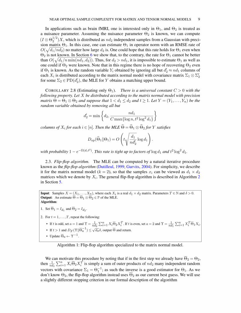
2.3. Flip-flop algorithm. The MLE can be computed by a natural iterative procedureknown as the flip-flop algorithm (Dutilleul, 1999; Gurvits, 2004). For simplicity, we describeit for the matrix normal model (k = 2), so that the samples xi can be viewed as d1 × d2
matrices which we denote by Xi. The general flip-flop algorithm is described in Algorithm 2in Section 5.
Input: Samples X = (X1, . . . ,Xn), where each Xi is a real d1 × d2 matrix. Parameters T ∈N and δ > 0.Output: An estimate Θ = Θ1 ⊗Θ2 ∈ P of the MLE.Algorithm:
1. Set Θ1 = Id1 and Θ2 = Id2 .
2. For t= 1, . . . , T , repeat the following:
• If t is odd, set a= 1 and Υ = 1nd2
∑ni=1XiΘ2X
Ti . If t is even, set a= 2 and Υ = 1
nd1
∑ni=1X
Ti Θ1Xi.
• If t > 1 and DF (Υ‖Θ−1a )≤
√daδ, output Θ and return.
• Update Θa←Υ−1.
Algorithm 1: Flip-flop algorithm specialized to the matrix normal model.
We can motivate this procedure by noting that if in the first step we already have Θ2 = Θ2,then 1
nd2
∑ni=1XiΘ2X
Ti is simply a sum of outer products of nd2 many independent random
vectors with covariance Σ1 = Θ−11 ; as such the inverse is a good estimator for Θ1. As we
don’t know Θ2, the flip-flop algorithm instead uses Θ2 as our current best guess. We will usea slightly different stopping criterion in our formal description of the algorithm
10 C. FRANKS, R. OLIVEIRA, A. RAMACHANDRAN AND M. WALTER
For the general tensor normal model, in each step the flip flop algorithm chooses one of thedimensions a ∈ [k] and uses the ath flattening of the samples xi (which are just Xi and XT
i inthe matrix case) to update Θa.
2.4. Results on the flip-flop algorithm. Our next results show that the flip-flop algorithmcan efficiently compute the MLE with high probability when the hypotheses of Theorem 2.4or Theorem 2.7 hold. We first state our result for the general tensor normal model and thengive an improved version for the matrix normal model. In the theorems that follow, we use thesame convention for choosing the Kronecker factors as in the preceding section.
THEOREM 2.9 (Tensor normal flip-flop). There are universal constants C,c > 0 such thatthe following holds. Suppose x = (x1, . . . , xn) are n ≥ Ck2d3
max/D independent samplesfrom the tensor normal model with precision matrix Θ = Θ1⊗· · ·⊗Θk . Then, with probabilityat least
1− k e−Ω( nD
k2d2max) − k2
(√nD
kdmax
)−Ω(dmin)
,
the MLE Θ exists, and for every 0< δ < c/√
(k+ 1)dmax, Algorithm 2 within
T =O
(k2dmax
(1 + logκ(Θ)
)+ k log
1
δ
)iterations outputs Θ with d(Θ, Θ)≤ 2δ and DF(Θa‖Θa)≤ 4
√da · δ for all a ∈ [k].
THEOREM 2.10 (Matrix normal flip-flop). There are universal constants C,c > 0 suchthat the following holds. Let 1< d1 ≤ d2. Suppose x1, . . . , xn ∈Rd1d2 are
n≥Cd2
d1max
logd2, log2 d1
independent samples from the matrix normal model with precision matrix Θ = Θ1⊗Θ2. Then,with probability at least 1−e−Ω(nd21/d2 log2 d1), the MLE Θ exists, and for every 0< δ < c/
√d2,
Algorithms 1 and 2 within
T =O
(d2
(1 + logκ(Θ)
)+ log
1
δ
)iterations outputs Θ with d(Θ, Θ) =O(δ) and DF(Θa‖Θa) =O(
√da · δ) for all a ∈ 1,2.
Plugging in the error rates for the MLE from Theorems 2.4 and 2.7 into Theo-rems 2.9 and 2.10 (with ε = 1) shows that the output of the flip-flop algorithm withO(k2dmax(1 + κ(Θ)) + k log(n)
)iterations is an efficiently computable estimator with the
same statistical guarantees as we have shown for the MLE.
3. Sample complexity for the tensor normal model. It was observed by Wiesel (2012)that the negative log-likelihood exhibits a certain variant of convexity known as geodesicconvexity. In this section, we use geodesic convexity, following a strategy similar to Franksand Moitra (2020), to prove Theorem 2.4. Our improved result for the matrix normal model,Theorem 2.7, requires additional tools and will be proved later in Section 4.
NEAR OPTIMAL SAMPLE COMPLEXITY FOR MATRIX AND TENSOR NORMAL MODELS 11
3.1. Geodesic convexity. We now discuss the geodesic convexity used here and outline thestrategy for our proof. We start by introducing a Riemannian metric on the manifold PD(D)of positive-definite real symmetric D×D matrices. Rather than simply considering the metricinduced by the Euclidean metric on the symmetric matrices, we consider the Riemannianmetric whose geodesics starting at a point Θ ∈ PD(D) are of the form t 7→ Θ1/2eHtΘ1/2
for t ∈R and a symmetric matrixH . This metric arises from the Hessian of the log-determinant(Bhatia, 2009) and also as the Fisher information metric on centered Gaussians parametrizedby their covariance matrices (Skovgaard, 1984). If Θ is positive definite and A an invertiblematrix then AΘAT is again positive definite. The transformation Θ 7→AΘAT is an isometrywith respect to this metric, i.e., it preserves the geodesic distance, as well as the statisticaldistancesDF andDop that we use (Definition 2.3). This invariance is natural because changinga pair of precision matrices in this way does not change the statistical relationship between thecorresponding Gaussians; in particular the total variation distance, Fisher-Rao, and Kullback-Leibler divergence are unchanged.
As observed by Wiesel (2012), the negative log-likelihood is convex as the precision matrixmoves along the geodesics of the Fisher information metric, and in particular for the tensornormal model it is convex along geodesics in P = Θ1⊗ . . .⊗Θk ∈ PD(d1)×· · ·×PD(dk).This is because the geodesics in PD(D) between elements of the manifold
P =
Θ = Θ1 ⊗ . . .⊗Θk : Θa ∈ PD(da)
remain in P. That is, P is a totally geodesic submanifold of PD(D). Its tangent space can beidentified with the real vector space
H =
(H0;H1, . . . ,Hk) : H0 ∈R, Ha a symmetric traceless da × da matrix∀a ∈ [k],
equipped with the norm and inner product
‖H‖F := 〈H,K〉1/2 , 〈H,K〉 :=H0K0 +
k∑a=1
TrHTa Ka.
The direction (1; 0, . . . ,0) changes Θ by an overall scalar, and tangent directions supportedonly in the ath component for a ∈ [k] only change Θa; subject to its determinant staying fixed.The geodesics on P are simply the geodesics of the Fisher-information metric on PD(D), butwe will define them precisely in terms of the tangent space H as follows to fix our conventions.
DEFINITION 3.1 (Exponential map and geodesics). The exponential map expΘ : H→ Pat Θ = Θ1 ⊗ · · · ⊗Θk ∈ P is defined by
expΘ(H) = eH0 · (Θ1/21 e
√d1H1Θ
1/21 )⊗ · · · ⊗ (Θ
1/2k e
√dkHkΘ
1/2k ).
By definition, the geodesics through Θ are the curves t 7→ expΘ(tH) for t ∈ R and H ∈H.Up to reparameterization, there is a unique geodesic between any two points of P.
We take the convention that the geodesics have unit speed if ‖H‖2F = 1. The geodesicdistance d(Θ,Θ′) between two points Θ and Θ′ = expΘ(H) is therefore equal to ‖H‖F ,which can also be computed as D−1/2‖log Θ−1/2Θ′Θ−1/2‖F . To summarize:
DEFINITION 3.2 (Geodesic distance and balls). The geodesic distance d(Θ,Θ′) betweentwo points Θ and Θ’ is given by
d(Θ,Θ′) =1√D‖log Θ−1/2Θ′Θ−1/2‖F =
√2
D· dFR(Θ,Θ′).(3.1)
12 C. FRANKS, R. OLIVEIRA, A. RAMACHANDRAN AND M. WALTER
where log denotes the matrix logarithm and dFR is the Fisher-Rao distance defined in Eq. (2.6).We choose the normalization in Eq. (3.1) because it will make the negative log-likelihoodfunctions typically Ω(1)-strongly convex, while ensuring that the gradients are O(1).
The closed (geodesic) ball of radius r > 0 about Θ is defined as
Br(Θ) =
expΘ(H) : ‖H‖F ≤ r,
The manifold PD(D), and hence P, is a Hadamard manifold, i.e., a complete, simplyconnected Riemannian manifold of non-positive sectional curvature (Bacák, 2014). Thusgeodesic balls are geodesically convex subsets of P, that is, if γ(t) is a geodesic suchthat γ(0), γ(1) ∈Br(Θ) then γ(t) ∈Br(Θ) for all t ∈ [0,1].
Using our definition of geodesics, we obtain the following notion of geodesic convexity offunctions.
DEFINITION 3.3 (Geodesic convexity). Given a geodesically convex domain D ⊆ P,we say that a function f is (strictly) geodesically convex on D if, and only if, the functiont 7→ f(γ(t)) is (strictly) convex on [0,1] for any geodesic γ(t) with γ(0), γ(1) ∈D. It is calledλ-strongly geodesically convex if t 7→ f(γ(t)) is λ-strongly convex along every unit-speedgeodesic γ with endpoints in D.
For a twice differentiable function f : P → R, we can ensure that it is λ-stronggeodesically convex on D by requiring that f is λ-strong geodesically convex at Θ, i.e.∂2t=0f(expΘ(tH))≥ λ‖H‖2F , for all H ∈H, for every Θ ∈D.
EXAMPLE 3.4. It is instructive to consider the case k = 1, or P = PD(D). The geodesicsthrough Θ are the curves t 7→
√ΘeHt
√Θ. As an example of a geodesically convex function,
consider the likelihood for the precision matrix of a Gaussian with data x1, . . . , xn. Letρ := 1
nD
∑i xix
Ti denote the matrix of “second sample moments” of the data. Then we can
rewrite the objective function (2.1) as
fx(Θ) = TrρΘ− 1
Dlog det Θ.
We claim that fx(Θ) is always geodesically convex, and in fact strictly geodesically convexwhenever ρ is invertible. Indeed,
∂2t=0fx(
√ΘetH
√Θ) = Tr
√Θρ√
ΘH2 ≥ 0
with strict inequality whenever ρ is invertible (and H nonzero).
The invariance properties described above for PD(D) are directly inherited to P. Themanifold P carries a natural action by the group
G = A=A1 ⊗ . . .⊗Ak : Ga ∈GL(da)
Namely, if Θ ∈ P and A ∈ G then the AΘAT is in P. Moreover, as discussed above, themapping Θ 7→ AΘAT is an isometry of the Riemannian manifold P and it preserves thestatistical distances DF and Dop.
3.2. Sketch of proof. With these definitions in place, we are able to state a proof planfor Theorem 2.4. The proof is a Riemannian version of the standard approach using strongconvexity.
NEAR OPTIMAL SAMPLE COMPLEXITY FOR MATRIX AND TENSOR NORMAL MODELS 13
1. Reduce to identity: We can obtain n independent samples from N (0,Θ−1) as x′i =
Θ−1/2xi, where x1, . . . , xn are distributed as n independent samples from a standardGaussian. The MLE Θ(x′) for the former is exactly Θ1/2Θ(x)Θ1/2. By invariance of therelative Frobenius error, DF(Θ(x′)‖Θ) =DF(Θ(x)‖ID); the same is true for Dop. Thisshows that to prove Theorem 2.4 it is enough to consider the case that Θ = ID, i.e., thestandard Gaussian.
2. Bound the gradient: Show that the gradient ∇fx(ID) (defined below) is small with highprobability.
3. Show strong convexity: Show that, with high probability, fx is Ω(1)-strongly geodesicallyconvex near I .
These together imply the desired sample complexity bounds – as in the Euclidean case,strong convexity in a suitably large ball about a point implies the optimizer cannot be far.Moreover, it happens that under alternating minimization fx obeys a descent lemma (similarto what is shown in Bürgisser et al. (2018)); as such the flip-flop algorithm must convergeexponentially quickly by the strong geodesic convexity of fx.
To make this discussion more concrete, we now define the gradient and Hessian formally,and state the lemma that we will use to relate the gradient and strong convexity to the distanceto the optimizer as in the plan above.
DEFINITION 3.5 (Gradient and Hessian). Let f : P→R be a once or twice differentiablefunction and Θ ∈ P. The (Riemannian) gradient ∇f(Θ) is the unique element in H such that
〈∇f(Θ),H〉= ∂t=0f(expΘ(tH)) ∀H ∈H.
Similarly, the (Riemannian) Hessian ∇2f(Θ) is the unique linear operator on H such that
〈H,∇2f(Θ)K〉= ∂s=0∂t=0f(expΘ(sH + tK)) ∀H,K ∈H.
We abbreviate∇f =∇f(ID) and∇2f =∇2f(ID) for the gradient and Hessian, respectively,at the identity matrix, and we write ∇af and ∇2
abf for the components. As block matrices,
∇f =
∇0f∇1f
...∇kf
, ∇2f =
∇2
00f ∇201f . . . ∇2
0kf∇2
10f ∇211f . . . ∇2
1kf...
.... . .
...∇2k0f ∇2
k1f . . . ∇2kkf
.Here,∇0f ∈R and each∇af(Θ) is a da×da traceless symmetric matrix. Similarly, for a, b ∈[k] (i.e., for the blocks of the submatrix to the lower-right of the lines) the components∇2
abf(Θ)of the Hessian are linear operators from the space of traceless symmetric db × db matrices tothe space of traceless symmetric da × da matrices, while ∇a0f is a linear operator from Rto the space of traceless symmetric da × da matrices (hence can itself be viewed as such amatrix), ∇0af is the adjoint of this linear operator, and ∇2
00f(Θ) is a real number.
We note that the Hessian is symmetric with respect to the inner product 〈·, ·〉 on H. Justlike in the Euclidean case, the Hessian is convenient to characterize strong convexity. Indeed,〈H,∇2f(Θ)H〉= ∂2
t=0f(expΘ(tH)) for all H ∈H. Thus, f is geodesically convex if andonly if the Hessian is positive semidefinite, that is, ∇2f(Θ) 0. Similarly, f is λ-stronglygeodesically convex if and only if ∇2f(Θ) λIH, i.e., the Hessian is positive definite witheigenvalues larger than or equal to λ.
We can now state and prove the following lemma, which shows that strong convexity in aball about a point where the gradient is sufficiently small implies the optimizer cannot be far.
14 C. FRANKS, R. OLIVEIRA, A. RAMACHANDRAN AND M. WALTER
LEMMA 3.6. Let f : P→R be geodesically convex and twice differentiable. Assume thegradient at some Θ ∈ P is bounded as ‖∇f(Θ)‖F ≤ δ, and that f is λ-strongly geodesicallyconvex in a ball Br(Θ) of radius r > 2δ
λ . Then the sublevel set Υ ∈ P : f(Υ) ≤ f(Θ) iscontained in the ball B2δ/λ(Θ), f has a unique minimizer Θ, this minimizer is contained inthe smaller ball Bδ/λ(Θ), and
f(Θ)≥ f(Θ)− δ2
2λ.(3.2)
PROOF. We first show that the sublevel set of f(Θ) is contained in the ball of radius 2δλ .
Consider g(t) := f(expΘ(tH)), where H ∈H is an arbitrary vector of unit norm ‖H‖F = 1.Then, using the assumption on the gradient,
g′(0) = ∂t=0f(expΘ(tH)) = 〈∇f(Θ),H〉 ≥ −‖∇f(Θ)‖F ‖H‖F ≥−δ.(3.3)
Since f is λ-strongly geodesically convex on Br(Θ), we have g′′(t) ≥ λ for all |t| ≤ r. Itfollows that for all 0≤ t≤ r we have
g(t)≥ g(0)− δt+1
2λt2.(3.4)
Plugging in t = r yields g(r) ≥ g(0) +(λr2 − δ
)r > g(0). Since g is convex due to the
geodesic convexity of f , it follows that, for any t≥ r,
g(0)< g(r)≤(
1− r
t
)g(0) +
r
tg(t),
hence
f(Θ) = g(0)< g(t) = f(expΘ(tH)).
Thus, since H was an arbitrary unit norm tangent vector, the sublevel set of f(Θ) is containedin the ball of radius r about Θ. By replacing r with any smaller r′ > 2δ
λ , we see that thesublevel set is in fact contained in the closed ball of radius 2δ
λ . In particular, the minimum of fis attained and any minimizer Θ is contained in this ball. Moreover, as the right-hand side ofEq. (3.4) takes a minimum at t= δ
λ , we have g(t)≥ g(0)− δ2
2λ for all 0≤ t≤ r. By definitionof g, this implies Eq. (3.2).
Next, we prove that any minimizer of f is necessarily contained in the ball of radius δλ . To
see this, take an arbitrary minimizer Θ and write it in the form Θ = expΘ(TH), where H ∈His a unit vector and T > 0.
As before, we consider the function g(t) = f(expΘ(tH)). Then, using Eq. (3.3), theconvexity of g(t) for all t ∈R and the λ-strong convexity of g(t) for |t| ≤ r, we have
0 = g′(T ) = g′(0) +
∫ T
0g′′(t)dt≥ λmin(T, r)− δ.
If T > r then we have a contradiction as λr−δ > λr/2−δ > 0. Therefore we must have T ≤ rand hence λT − δ ≤ 0, so T ≤ δ
λ . Thus we have proved that any minimizer of f is containedin the ball of radius δ
λ .We still need to show that the minimizer is unique; that this follows from strong convexity is
convex optimization “folklore,” but we include a proof nonetheless. Indeed, suppose that Θ is aminimizer and let H ∈H be arbitrary. Consider h(t) := f(expΘ(tH)). Then the function h(t)is convex, has a minimum at t= 0, and satisfies h′′(0)> 0, since f is λ-strongly geodesicallyconvex near Θ, as Θ ∈ Br(Θ) by what we showed above. It follows that h(t) > h(0) forany t 6= 0. Since H was arbitrary, this shows that f(Υ)> f(Θ) for any Υ 6= Θ.
NEAR OPTIMAL SAMPLE COMPLEXITY FOR MATRIX AND TENSOR NORMAL MODELS 15
Using the geodesic distance bounds from the previous lemma allows us to obtain boundson the statistical distance measures DF and Dop of the overall precision matrix as well as ofthe individual Kronecker factors, assuming strong convexity.
LEMMA 3.7 (From geodesic distance toDF,Dop). Suppose the geodesic distance betweenΘ,Θ ∈ P satisfies d(Θ,Θ) ≤ δ for δ ≤ 1/
√dmax. Writing Θ = Θ1 ⊗ · · · ⊗ Θk and Θ =
Θ1⊗· · ·⊗Θk with (det Θ1)1/d1 = . . .= (det Θk)1/dk and (det Θ1)1/d1 = . . .= (det Θk)
1/dk ,we have
Dop(Θa‖Θa)≤DF(Θa‖Θa)≤ 2√da · δ
and
Dop(Θ‖Θ)≤DF(Θ‖Θ)≤ 2k√D · δ e2kδ.
PROOF. It suffices to prove the bounds for DF. By the invariance of DF and the geodesicdistance, we may assume that Θ = ID, i.e., Θa = Ia for all a ∈ [k]. By our assumption onthe geodesic distance, we may write Θ = expID(H) for H ∈H and ‖H‖F ≤ δ. Then by ourconvention, the Kronecker factors are given by
Θa = eH0k · e
√daHa = e
H0kIda+
√daHa
for all a ∈ [k], since Ha is traceless. Note that for each a ∈ [k] we have
‖H0
kIda +
√daHa‖2F =
1
k2|H0|2da + da‖Ha‖2F ≤ da‖H‖2F ≤ daδ2.
By assumption, the above is at most one, so by Fact B.1 we obtain
DF(Θa‖Ia) = ‖Ia − Θa‖F = ‖Ia − eH0kIda+
√daHa‖F
≤ 2‖H0
kIda +
√daHa‖F ≤ 2
√da · δ,
which establishes the first bound. The second now follows easily by a telescoping sum:
DF(Θ‖ID) = ‖Id1 ⊗ · · · ⊗ Idk − Θ1 ⊗ · · · ⊗ Θk‖F
≤k∑a=1
‖Θ1‖F · · · ‖Θa−1‖F ‖Ida − Θa‖F ‖Ida+1‖F · · · ‖Idk‖F
≤ 2√D · δ
k∑a=1
(1 + 2δ)a−1 ≤ 2k√D · δ e2kδ.
3.3. Bounding the gradient. Proceeding according to step 2 of the plan outlined in Sec-tion 3.2, we now compute the gradient of the objective function and bound it using matrixconcentration results.
To calculate the gradient, we need a definition from linear algebra. Recall that our datacomes as an n-tuple x= (x1, . . . , xn) of k-tensors. As in Example 3.4, let ρ := 1
nD
∑i xix
Ti
denote the “second sample moments”, and rewrite the objective function (2.1) as
fx(Θ) = TrρΘ− 1
Dlog det Θ.(3.5)
We may also consider the “second sample moments” of a subset of the coordinates J ⊆ [k].For this the following definition is useful.
16 C. FRANKS, R. OLIVEIRA, A. RAMACHANDRAN AND M. WALTER
DEFINITION 3.8 (Partial trace). Let ρ be an operator on Rd1 ⊗ . . .⊗Rdk , and J ⊆ [k]an ordered subset. Define the partial trace ρ(J) as the dJ × dJ -matrix, dJ =
∏a∈J da, that
satisfies the property that
Trρ(J)H = TrρH(J)(3.6)
for any dJ × dJ matrix H , where H(J) denotes the operator on Rd1 ⊗ · · · ⊗ Rdk that actsas H on the tensor factors labeled by J (in the order determined by J ) and as the identity onthe rest. This property uniquely determines ρ(J). We write ρ(a) and ρ(ab) when J = a andJ = a, b, respectively.
If ρ is positive (semi)definite then so is ρ(J). Moreover, Trρ= Trρ(J) and (ρ(J))(K) = ρ(K)
for K ⊆ J .Concretely, the partial trace ρ(J) can be calculated as follows: Analogously to the discussion
in Section 2.1, “flatten” the data x by regarding it as a dJ ×NJ matrix x(J), where NJ = nDdJ
;then ρ(J) = 1
nDx(J)(x(J))T .
The components of the gradient can be readily computed in terms of partial traces.
LEMMA 3.9 (Gradient). Let ρ = 1nD
∑ni=1 xix
Ti . Then the components of the gradi-
ent ∇fx at the identity are given by
∇afx =√da
(ρ(a) − Trρ
daIda
)for a ∈ [k],(3.7)
∇0fx = Trρ− 1.(3.8)
PROOF. For all a ∈ [k] and any traceless symmetric da × da matrix H , we have
〈∇afx(ID),H〉= ∂t=0fx(et√daH(a)) = ∂t=0
(Trρet
√daH(a) − 1
Dlog det(et
√daH(a))
)=√daTrρH(a) =
√daTrρ(a)H
using Eqs. (3.5) and (3.6) and that TrH(a) = 0 since TrH = 0. Since ∇afx is traceless andsymmetric by definition, while ρ(a) is symmetric, this implies that ∇ffx is the orthogonalprojection of ρ(a) onto the traceless matrices, i.e.,
∇afx =√da
(ρ(a) − Trρ(a)
daIda
)=√da
(ρ(a) − Trρ
daIda
).
Finally,
∇0fx = ∂t=0
(Trρet − 1
Dlog det(etID)
)= ∂t=0
(Trρet − t
)= Trρ− 1.
REMARK 3.10 (Gradient at other points from equivariance). In the previous lemmawe only computed the gradient at the identity. However, this is without loss of generality,since from the calculations above one easily obtains ∇fx(Θ) = ∇fΘ1/2x(I). That is, thegradient ∇fx(Θ) is given by Eqs. (3.7) and (3.8) with ρ replaced by Θ1/2ρΘ1/2.
Having calculated the gradient of the objective function, we are ready to state our bound:
NEAR OPTIMAL SAMPLE COMPLEXITY FOR MATRIX AND TENSOR NORMAL MODELS 17
PROPOSITION 3.11 (Gradient bound). Let x= (x1, . . . , xn) consist of independent stan-dard Gaussian random variables in RD. Suppose that 0 < ε < 1 and n ≥ d2max
Dε2 . Then, the
following occurs with probability at least 1− 2(k+ 1)e−ε2 nD
8dmax :
‖∇afx‖op ≤9ε√da
for all a ∈ [k],
|∇0fx| ≤ ε.As a consequence,
‖∇fx‖2F ≤ (1 + 81k)ε2 ≤ 82kε2.
To prove this we will need a standard result in matrix concentration. By the discussion belowDefinition 3.8, when the samples x= (x1, . . . , xn) are independent standard Gaussians in RD ,then ρ(a) is distributed as 1
nDY YT , where Y is a random da ×Na matrix with independent
standard Gaussian entries, where Na = nDda
. The following result bounds the singular valuesof such random matrices.
THEOREM 3.12 (Corollary 5.35 of Vershynin (2012)). Let Y ∈Rd×N have independentstandard Gaussian entries where N ≥ d. Then, for every t > 0, the following occurs withprobability at least 1− 2e−t
2/2:√N −
√d− t≤ σd(Y )≤ σ1(Y )≤
√N +
√d+ t,
where σj denotes the j-th largest singular value.
We will also need to bound Trρ= 1nD‖x‖
22. Because ‖x‖22 is simply a sum of nD many
χ2 random variables, the next proposition follows from standard concentration bounds.
PROPOSITION 3.13 (Example 2.11 of Wainwright (2019)). Let x= (x1, . . . , xn) consistof independent standard Gaussian random variables in RD . Then, for 0< t < 1, the followingoccurs with probability at least 1− 2e−t
2nD/8:
(1− t)nD ≤ ‖x‖22 ≤ (1 + t)nD.
Equipped with these results we now prove our gradient bound.
PROOF OF PROPOSITION 3.11. For any fixed a ∈ [k], recall that ρ(a) has the same distribu-tion as 1
nDY YT , where Y is a da×Na-matrix with standard Gaussian entries whereNa = nD
da.
By Theorem 3.12, we have the following bound with failure probability at most 2e−t2/2:√
Na −√da − t≤ σd(Y )≤ σ1(Y )≤
√Na +
√da + t.
This event tells us that the eigenvalues of daρ(a) are in the range ((1−√da+t√Na
)2, (1+√da+t√Na
)2).
Let t = ε√nD/da = ε
√Na. Because n ≥ d2
max/Dε2 and 0 < ε ≤ 1, we have
√da ≤ t ≤√
Na. Hence, the eigenvalues of daρ(a) are contained in (1− 4 t√Na,1 + 8 t√
Na), and so the
eigenvalues of daρa − Ida are bounded in absolute value by 8ε with failure probability atmost 2e−ε
2nD/2da . Moreover, by Proposition 3.13, we have that |Trρ− 1| ≤ ε with failureprobability at most 2e−ε
2nD/8. The formulae in Lemma 3.9 and the union bound imply
‖∇afx‖op ≤1√da
∥∥∥daρ(a) − Ida∥∥∥
op+|Trρ− 1|√
da≤ 8ε√
da+
ε√da≤ 9ε√
da
for all a ∈ [k], as well as
|∇0fx|= |Trρ− 1| ≤ ε,
with failure probability at most 2(k+ 1)e−ε2nD/8dmax .
18 C. FRANKS, R. OLIVEIRA, A. RAMACHANDRAN AND M. WALTER
3.4. Strong convexity from expansion. In this section, we prove our strong convexityresult, Proposition 3.21, in order to carry out step 3 of the plan from Section 3.2. The theoremstates that, with high probability, fx is strongly convex near the identity. We will prove it byfirst establishing strong convexity at the identity, Proposition 3.19, using quantum expansiontechniques, and then giving a bound on how the Hessian changes away from the origin,Lemma 3.20. We then combine these results to prove Proposition 3.21 at the end of thissubsection.
Similarly as for the gradient, we can compute the components of the Hessian in terms ofpartial traces, but now we also need to consider two coordinates at a time.
LEMMA 3.14 (Hessian). Let ρ = 1nD
∑ni=1 xix
Ti . Then the components of the Hes-
sian ∇2fx at the identity are given by
〈H, (∇2aafx)H〉= daTrρ(a)H2
〈H, (∇2abfx)K〉=
√dadbTrρ(ab) (H ⊗K)
for all a 6= b ∈ [k] and traceless symmetric da × da matrices H , db × db matrices K , and
∇20afx =
√da
(ρ(a) − Trρ
daIda
)= ∇2
a0fx,
∇200fx = Trρ.
for all a ∈ [k].
Here we use the conventions discussed in Definition 3.5. In particular, we identify ∇2a0fx,
which is a linear operator from the real numbers to the traceless symmetric matrices, with atraceless symmetric matrix, and similarly for its adjoint ∇2
0afx. The notation = reminds us ofthese identifications.
PROOF. Note that the Hessian of fx coincides with the one of TrρΘ. This follows fromEq. (3.5), since the Hessian of log det Θ vanishes identically. Accordingly, we will computethe Hessian of TrρΘ. For a ∈ [k] and any traceless symmetric da × da matrix H , we have
〈H, (∇2aafx)H〉= ∂s=0∂t=0 Trρe(s+t)
√daH(a) = daTrρH2
(a) = daTrρ(a)H2
using Eq. (3.6). Similarly, for a 6= b ∈ [k], any traceless symmetric da × da matrix H , and anytraceless symmetric db × db matrix K , we find that
〈H, (∇2abfx)K〉= ∂s=0∂t=0 Trρes
√daH(a)+t
√dbK(b)
=√dadbTrρH(a)K(b) =
√dadbTrρ(ab) (H ⊗K)
using Eq. (3.6). Next, for a ∈ [k] and any traceless symmetric da × da matrix H , we have
〈H,∇2a0fx〉= ∂s=0∂t=0 Trρes
√daH(a)+t =
√daTrρH(a) =
√daTrρ(a)H.
As we identify ∇2a0fx with a traceless symmetric da × da matrix; this shows that
∇2a0fx =
√da
(ρ(a) − Trρ
daIda
),
and similarly for the transpose. Finally,
∇200fx = ∂s=0∂t=0 Trρes+t = Trρ.
NEAR OPTIMAL SAMPLE COMPLEXITY FOR MATRIX AND TENSOR NORMAL MODELS 19
REMARK 3.15 (Hessian at other points from equivariance). Analogously to Remark 3.10,we can compute the Hessian at other points using ∇2fx(Θ) =∇2fΘ1/2x. That is, the Hes-sian ∇2fx(Θ) is given by Lemma 3.14 with ρ replaced by Θ1/2ρΘ1/2.
The most interesting part of the Hessian are the off-diagonal components for a 6= b ∈ [k],which up to an overall factor
√dadb can be seen as the restrictions of the linear maps
Φ(ab) : Mat(db)→Mat(da), 〈H,Φ(ab)(K)〉= Trρ(ab) (H ⊗K)(3.9)
to the traceless symmetric matrices. Equation (3.9) is a special case of a completely positivemap, which is a linear map of the form
ΦA : Mat(db)→Mat(da), ΦA(X) =
N∑i=1
AiXATi(3.10)
for da × db matrices A1, . . . ,AN . To see the connection, note that since ρ(ab) is positivesemidefinite, it can be written in the form
∑Ni=1 vec(Ai) vec(Ai)
T ; then Φ(ab) = ΦA follows.The matrices A1, . . . ,AN are known as Kraus operators. Equation (3.10) can also be writtenas
vec(ΦA(X)) =
N∑i=1
(Ai ⊗Ai) vec(X).(3.11)
We denote by Φ∗ : Mat(da)→Mat(db) the adjoint of a completely positive map Φ withrespect to the Hilbert-Schmidt inner product; this is again a completely positive map, withKraus operators AT1 , . . . ,A
TN . In our proof of strong convexity, we will show that strong
convexity follows if the completely positive maps Φ(ab) are good quantum expanders.
DEFINITION 3.16 (Quantum expansion). Let Φ: Mat(db)→Mat(da) be a completelypositive map. Say Φ is ε-doubly balanced if∥∥∥∥ Φ(Idb)
Tr Φ(Idb)− Idada
∥∥∥∥op
≤ ε
daand
∥∥∥∥ Φ∗(Ida)
Tr Φ∗(Ida)− Idbdb
∥∥∥∥op
≤ ε
db.(3.12)
The map Φ is an (ε, η)-quantum expander if Φ is ε-doubly balanced and
‖Φ‖0 := maxH traceless symmetric
‖H‖F=1
‖Φ(H)‖F ≤ ηTr Φ(Idb)√
dadb(3.13)
A (0, η)-quantum expander is called a η-quantum expander.
Quantum expanders originate in quantum information theory and quantum computation Hast-ings (2007). There one typically takes da = db and ε = 0, so that Eq. (3.13) simplifiesto ‖Φ‖0 ≤ η. Definition 3.16 is invariant under rescaling Φ 7→ cΦ for c > 0. Here we followthe definitions of Kwok, Lau and Ramachandran (2019); Franks and Moitra (2020), whorecognized the connection between the quantum expansion and spectral gaps of the Hessianfor operator scaling (but we note that some of the following can be slightly simplified if oneopts for a non-scale invariant definition). For us, the following lemma will allow us to translatequantum expansion properties into strong convexity.
LEMMA 3.17 (Strong convexity from expansion). If the completely positive maps Φ(ab)
defined in Eq. (3.9) are (ε, η)-quantum expanders for every a 6= b ∈ [k], then∥∥∥∥∇2fxTrρ
− IH∥∥∥∥
op
≤ (k− 1)η+ (√k+ 1)ε.
Assuming k ≥ 2, the right-hand side is at most k(η+ ε).
20 C. FRANKS, R. OLIVEIRA, A. RAMACHANDRAN AND M. WALTER
It suffices to verify the hypothesis for a < b. Indeed, since Tr Φ∗(Ida) = Tr Φ(Idb), any Φ isan (ε, η)-quantum expander if and only if this is the case for the adjoint Φ∗, but note that theadjoint of Φ(ab) is Φ(ba). To prepare the proof, we also note that
Φ(ab)(Idb) = ρ(a) and (Φ(ab))∗(Ida) = Φ(ba)(Ida) = ρ(b),(3.14)
hence in particular Tr Φ(ab)(Idb) = Trρ.
PROOF. We wish to bound the operator norm of M = ∇2fxTrρ − IH, which we consider as a
block matrix as in Definition 3.5. For this, we use the following basic estimate of the norm ofa block matrix in terms of the norm of the matrix of block norms:
‖M‖op ≤ ‖m‖op, where m= (‖Mab‖op)a,b∈0,1,...,k.(3.15)
We first bound the individual block norms, using that the blocks can be computed usingLemma 3.14. Recall that the off-diagonal blocks of the Hessian, ∇2
abfx for a 6= b ∈ [k], aregiven by the restriction of
√dadbΦ
(ab) to the traceless symmetric matrices. Since Φ(ab) is an(ε, η)-quantum expander, we have
‖Mab‖op =‖∇2
abfx‖op
Trρ=
√dadb
Tr Φ(ab)(Idb)‖Φ(ab)‖0 ≤ η,
using that Tr Φ(ab)(Idb) = Trρ. The remaining off-diagonal blocks can be bounded as
‖Ma0‖=‖∇2
a0fx‖op
Trρ=
∥∥∥∥√da( ρ(a)
Trρ− Idada
)∥∥∥∥F
=√da
∥∥∥∥ Φ(ab)(Idb)
Tr Φ(ab)(Idb)− Idada
∥∥∥∥F
≤ da∥∥∥∥ Φ(ab)(Idb)
Tr Φ(ab)(Idb)− Idada
∥∥∥∥op
≤ ε,
using the fact that the operator norm of a linear functional 〈K,−〉 is the same as the Frobeniusnorm of K , and Eq. (3.14). On the other hand, the diagonal blocks for a ∈ [k] can be boundedby observing that, for any traceless Hermitian H ,
|〈H,MaaH〉|=∣∣∣∣〈H,(∇2
aafxTrρ
− I)H〉∣∣∣∣= da
∣∣∣∣Tr
(ρ(a)
Trρ− Idada
)H2
∣∣∣∣≤ da
∥∥∥∥ ρ(a)
Trρ− Idada
∥∥∥∥op
‖H‖2F ≤ ε‖H‖2F ,
hence ‖Maa‖op ≤ ε, while |M00|= |∇200fx
Trρ − 1|= 0. To conclude the proof, decompose
m=
0 0 0 · · · 00 0 m12 · · · m1k
0 m21 0 m2k...
.... . .
...0mk1 mk2 · · · 0
+
0 0 0 · · · 00m11 0 · · · 00 0 m22 0...
.... . .
...0 0 0 · · · mkk
+
0 m01 m02 · · · m0k
m10 0 0 · · · 0m20 0 0 0
......
. . ....
mk0 0 0 · · · 0
.The nonzero entries of the first matrix are bounded by η, hence its operator norm is at most(k− 1)η. The second matrix is diagonal with diagonal entries bounded by ε, hence its operatornorm is at most ε. The third matrix has nonzero entries bounded by ε, hence its operator normis bounded by
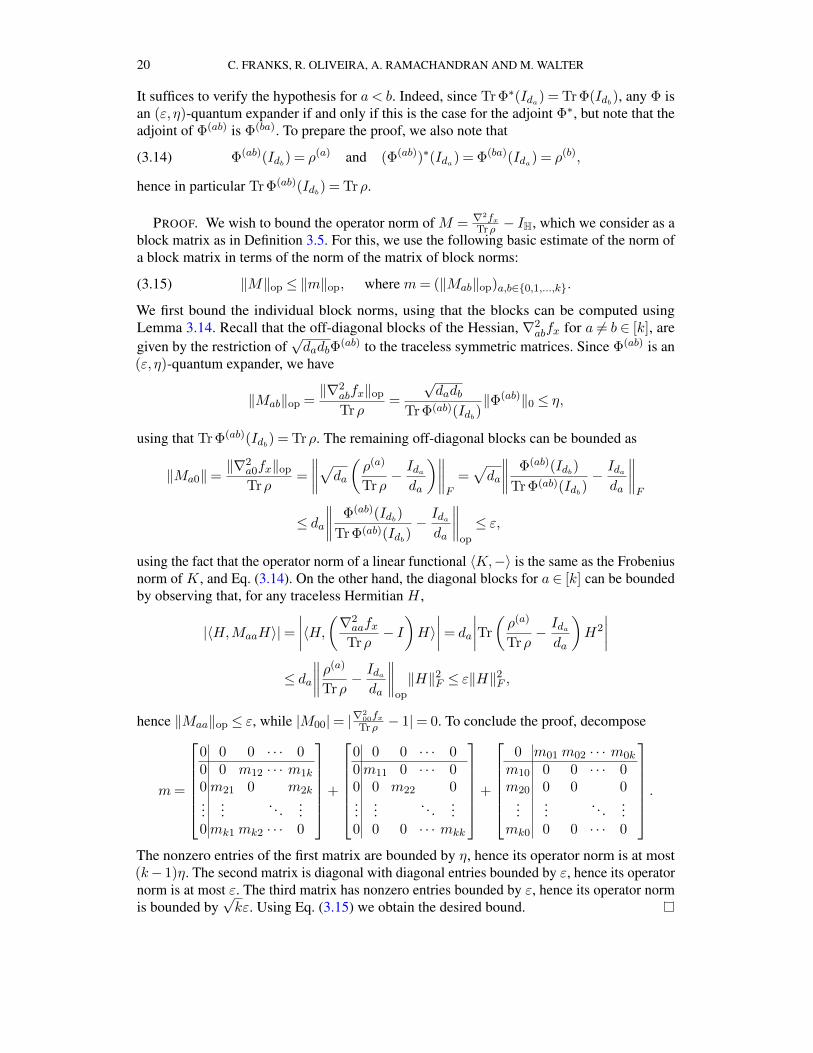
√kε. Using Eq. (3.15) we obtain the desired bound.
NEAR OPTIMAL SAMPLE COMPLEXITY FOR MATRIX AND TENSOR NORMAL MODELS 21
We are concerned with Φ(ab) that arise from random Gaussians. Just like random graphscan give rise to good expanders, it is known that random completely positive maps, namely Φconstructed by choosing Kraus operators at random from well-behaved distributions, yieldgood quantum expanders. When the Kraus operators are chosen to be standard Gaussian wehave the following result:
THEOREM 3.18 (Pisier (2012, 2014)). Let A1, . . . ,AN be independent da × db randommatrices with independent standard Gaussian entries. Then, for every t≥ 2, with probabilityat least 1− t−Ω(da+db), the completely positive map ΦA, defined as in Eq. (3.10), satisfies
‖ΦA‖0 ≤O(t2√N (da + db)
).
Pisier’s actual result is slightly different. We present the details in Appendix A.When the samples x= (x1, . . . , xn) are independent standard Gaussians in RD , the random
completely positive maps Φ(ab) we are interested in have the same distribution as 1nDΦA, where
the Kraus operators A1, . . . ,AN are da × db matrices with independent standard Gaussianentries and N = nD
dadb. Accordingly, strong convexity at the identity follows quite easily from
Theorem 3.18 once double balancedness can be controlled. For the latter, observe that∥∥∥∥ Φ(ab)(Idb)
Tr Φ(ab)(Idb)− Idada
∥∥∥∥op
=1
Trρ
∥∥∥∥ρ(a) − Trρ
daIda
∥∥∥∥op
=1
1 +∇0fx
1√da‖∇afx‖op,
by Lemma 3.9, and similarly for the adjoint. Therefore, the completely positive maps Φ(ab)
are ε-doubly balanced if and only if, for all a ∈ [k],√da‖∇afx‖op ≤ εTrρ= (1 +∇0fx)ε,(3.16)
hence double balancedness can be controlled using the gradient bounds in Proposition 3.11.We now state and prove our strong convexity result at the identity:
PROPOSITION 3.19 (Strong convexity at identity). There is a universal constant C > 0such that the following holds. Let x= (x1, . . . , xn) be independent standard Gaussian randomvariables in RD , where n≥Ck d
2max
D . Then, with probability at least 1− k2(√nD
kdmax)−Ω(dmin),
‖∇2fx − IH‖op ≤1
4;
in particular, fx is 34 -strongly convex at the identity.
PROOF. By Lemma 3.17, it is enough to prove that with the desired probability all Φ(ab)
are (ε, η) := ( 140k1/2 ,
120k )-quantum expanders for a 6= b ∈ [k] and Trρ ∈ (7
8 ,98). If that is the
case, then ∥∥∇2fx − IH∥∥
op≤Trρ ·
∥∥∥∥∇2fxTrρ
− IH∥∥∥∥
op
+ |1−Trρ|
≤(
(k− 1)η+ (√k+ 1)ε
)Trρ+ |1−Trρ| ≤ 1
4.
Firstly, Trρ= 1nD‖X‖
2 is in (78 ,
98) with failure probability e−Ω(nD) by Proposition 3.13.
Next, we describe an event that implies the Φ(ab) are all ε-doubly balanced for ε= 140k1/2 .
By Eq. (3.16), this is equivalent to the condition√da‖∇afx‖op ≤ εTrρ for all a ∈ [k]. By
Proposition 3.11, and assuming the bound Trρ≥ 78 from above, the latter occurs with failure
probability ke−Ω( nD
kdmax) provided n≥Ck d
2max
D for a universal constant C > 0.
22 C. FRANKS, R. OLIVEIRA, A. RAMACHANDRAN AND M. WALTER
Finally, we describe an event that ensures that ‖Φ(ab)‖0 ≤ η Trρ√dadb
for η = 120k for any
fixed a 6= b, which is the other condition needed for quantum expansion. Recall that each Φ(ab)
is distributed as 1nDΦA, where A is a tuple of nD
dadbmany da × db matrices with independent
standard Gaussian entries. Thus, taking t2 =O(η√nD
da+db) and again assuming that Trρ≥ 7
8 , wehave ‖Φ(ab)‖0 ≤ η Trρ√
dadbby Theorem 3.18, with failure probability at most (
√nD
kdmax)−Ω(dmin).
By the union bound, we conclude that all Φ(ab) for a 6= b are (ε, η)-quantum expanders andthat Trρ ∈ (7
8 ,98), up to a failure probability of at most
e−Ω(nD) + ke−Ω(
nD
kdmax
)+ k2
(√nD
kdmax
)−Ω(dmin)
.
The final term dominates, which implies the desired failure probability. To see that the finalterm dominates compare exponents: it suffices to show that nD/kdmax ≥ dmin log(
√nD
kdmax) by
our assumption on n, which states that α := nD/kd2max ≥C . Writing the desired inequality
in terms of α, we need dmaxα≥ dmin log(√α/k). This holds for C large enough.
We now show our second strong convexity result, namely that if our function is stronglyconvex at the identity then it is also strongly convex in an operator norm ball about the identity.For this, we define
dop(A,B) := ‖logB−1/2AB−1/2‖op,(3.17)
which is a metric on PD(D) and hence also on P (cf. Eq. (3.1)). Then we have the followingresult, which we prove in Appendix B.
LEMMA 3.20 (Robustness of strong convexity). There is a universal constant 0< ε0 < 1such that if ‖∇afx(ID)‖op ≤ ε0/
√da for all a ∈ [k] and |∇0fx(ID)| ≤ ε0, then
‖∇2fx(Θ)−∇2fx‖op =O(δ)
for any Θ ∈ P such that δ := dop(Θ, ID)≤ ε0. In particular, for any λ > 0, if fx is λ-stronglyconvex at ID then fx is (λ−O(δ))-strongly convex at Θ.
Finally we obtain our strong convexity result near the identity.
PROPOSITION 3.21 (Strong convexity near identity). There are constants C,c > 0 suchthat the following holds. Let x = (x1, . . . , xn) be independent standard Gaussian randomvariables in RD, where n≥ Ck d
2max
D . Then, with probability at least 1− k2(√nD
kdmax)−Ω(dmin),
the function fx is 12 -strongly convex at any point Θ ∈ P such that dop(Θ, ID)≤ c.
PROOF. We can choose C > 0 such that both Propositions 3.11 and 3.19 apply (the formerwith ε≤ ε0/9 , where ε0 is the universal constant from Lemma 3.20). Then the assumptionsof Lemma 3.20 are satisfied for λ= 3
4 with failure probability at most
2(k+ 1)e−ε2 nD
8dmax + k2
(√nD
kdmax
)−Ω(dmin)
,
where the latter term dominates, and there exists a constant 0< c≤ ε0 such that f is 12 -strongly
convex at any point Θ such that dop(Θ, ID)≤ c.
NEAR OPTIMAL SAMPLE COMPLEXITY FOR MATRIX AND TENSOR NORMAL MODELS 23
REMARK 3.22. While Proposition 3.21 uses dop to quantify closeness to the identity, wecan easily translate it into a statement in terms of the geodesic distance. Namely, under thesame hypotheses it holds that fx is 1
2 -strongly convex on the geodesic ball Br(ID) of radius
r =c√
(k+ 1)dmax
,
where c > 0 is the universal constant from Proposition 3.21. Indeed, if Θ = expID(H), then
‖log Θ‖op ≤ |H0|+k∑a=1
√da‖Ha‖op ≤
√dmax
(|H0|+
k∑a=1
‖Ha‖op
)
≤√dmax
(|H0|+
k∑a=1
‖Ha‖F
)≤√dmax
√k+ 1‖H‖F ,
so if d(Θ, ID) = ‖H‖F ≤ r, then dop(Θ, ID) = ‖log Θ‖op ≤ c.
3.5. Proof of Theorem 2.4. We are now ready to prove the main result of this sectionaccording to the plan outlined in Section 3.2. We first state a result that bounds the geodesicdistance between the precision matrix and the MLE. The theorem then follows from boundsfor Dop and DF in terms of geodesic distance.
PROPOSITION 3.23 (Tensor normal geodesic error). There is a universal constant C > 0such that the following holds. Suppose that t≥ 1 and
n≥Ck2d3max
Dt2.(3.18)
Then the MLE Θ for n independent samples of the tensor normal model with precisionmatrix Θ satisfies
d(Θ,Θ) =O
(√k dmax√nD
t
),
with probability at least
1− ke−Ω(t2dmax
)− k2
(√nD
kdmax
)−Ω(dmin)
.
PROOF. By step 1 in Section 3.2, it is enough to prove the theorem assuming Θ = ID.Assuming this, we now show that the minimizer of fx exists and is close to Θ = ID withhigh probability. Let c > 0 be the constant from Proposition 3.21. Consider the following twoevents:
1. ‖∇fx‖F ≤ δ :=√
82k dmax√nDt.
2. fx is λ-strongly convex on the geodesic ball Br(ID), where λ = 12 and radius r :=
c√(k+1)dmax
.
Now, Proposition 3.11 (with ε = δ√82k
) shows that, assuming δ√82k
< 1 and n ≥ d2max
D( δ√82k
)2,
that is, n > d2max
D t2 and t≥ 1, the first event holds up to a failure probability of at most
2(k+ 1)e−( δ√82k
)2 nD
8dmax = ke−Ω(t2dmax).
24 C. FRANKS, R. OLIVEIRA, A. RAMACHANDRAN AND M. WALTER
On the other hand, Proposition 3.21 and Remark 3.22 show that, assuming n≥Ck d2max
D for auniversal constant C > 0, the second event holds up to a failure probability of at most
k2
(√nD
kdmax
)−Ω(dmin)
.
Note that both assumptions follow from Eq. (3.18) for some appropriate choice of C . Thus,by the above and the union bound, both events hold simultaneously with the advertisedsuccess probability. For C large enough, Eq. (3.18) moreover implies r > 2δ
λ , since the latteris equivalent to
n >16 · 82
c2k(k+ 1)
d3max
Dt2.
Thus, if the above two events hold, Lemma 3.6 applies (with our choice of δ and λ) and showsthat the MLE Θ exists, is unique, and has geodesic distance at most δλ = 2δ from Θ = ID .
The theorem now follows as a corollary. We restate it for convenience.
THEOREM 2.4 (Tensor normal Frobenius error, restated). There is a universal con-stant C > 0 such that the following holds. Suppose t≥ 1 and
(2.5) n≥Ck2d2max
Dmaxk, dmaxt2.
Then the MLE Θ = Θ1⊗ · · ·⊗ Θk for n independent samples of the tensor normal model withprecision matrix Θ = Θ1 ⊗ · · · ⊗Θk satisfies
DF(Θa‖Θa) =O
(t k1/2dmax
√danD
)for all a ∈ [k]
and DF(Θ‖Θ) =O
(t k3/2dmax√
n
),
with probability at least
1− ke−Ω(t2dmax
)− k2
(√nD
kdmax
)−Ω(dmin)
.
PROOF. By Proposition 3.23, noting that Eq. (2.5) implies Eq. (3.18), we have withthe desired failure probablity that Θ is at most geodesic distance δ from Θ, where δ =O(√k dmaxt/
√nD). Moreover, Eq. (3.18) also implies δ ≤ 1/
√dmax if we choose C large
enough. Thus, Lemma 3.7 applies, and we have that for each a ∈ [k],
DF(Θa‖Θa)≤ 2√da · δ =O
(t k1/2dmax
√danD
)as well as
DF(Θ‖Θ)≤ 2k√D · δ e2kδ =O
(t k3/2dmax√
n
).
In the last step, we used that δk = O(1), which also follows from Eq. (2.5). Indeed, it isequivalent to n≥C ′k3 d
2max
D t2 for some C ′ > 0.
NEAR OPTIMAL SAMPLE COMPLEXITY FOR MATRIX AND TENSOR NORMAL MODELS 25
4. Improvements for the matrix normal model. We now prove Theorem 2.7, whichimproves over Theorem 2.4 in the case of the matrix normal model (k = 2). Throughout thissection we assume without loss of generality that d1 ≤ d2. Our results for the matrix normalmodel are stronger in that:
1. the MLE is shown to be close to the truth in spectral norm (Dop) rather than the looserFrobenius norm (DF),
2. the errors are tight for the individual factors, and3. the failure probability is inverse exponential in the number of samples rather than inverse
polynomial.
4.1. Spectral gap and expansion. The proof plan is similar to that in Section 3.2, the maindifference being that we now work directly with quantum expansion instead of translating intostrong convexity. An important tool will be a bound by Kwok, Lau and Ramachandran (2019)which uses the notion of a spectral gap, which is closely related to quantum expansion.
DEFINITION 4.1 (Spectral gap). Let Φ: Mat(db)→Mat(da) be a completely positivemap. Say Φ has spectral gap γ > 0 if
σ2(Φ)≤ (1− γ)Tr Φ(Idb)√
dadb(4.1)
where σ2 denotes the second largest singular value of Φ. Note that γ ≤ 1. Moreover, thedefinition is invariant under rescaling Φ 7→ cΦ for c > 0.
Recall that by the variational formula for singular values, if we let K ∈Mat(db) be thefirst (right) singular vector of Φ, we can rewrite the above condition as
σ2(Φ) = max〈H,K〉=0
‖Φ(H)‖F‖H‖F
≤ (1− γ)Tr Φ(Idb)√
dadb.
On the other hand, the definition of an (ε, η)-quantum expander is given in Eq. (3.13) as
‖Φ‖0 := max〈H,Idb 〉=0
‖Φ(H)‖F‖H‖F
≤ ηTr Φ(Idb)√dadb
.
Due to the ε-doubly balanced condition in Eq. (3.12), it turns out that these two notions areclosely related, as the following lemma shows.
LEMMA 4.2 (Lemma A.3 in Franks and Moitra (2020)). There exists a universal con-stant c > 0 with the following property. If Φ is an (ε, η)-quantum expander and ε≤ c(1− η),then Φ has spectral gap 1− η−O(ε).
We now state the bound of Kwok, Lau and Ramachandran (2019) in our language. Be-cause k = 2, the gradient and Hessian are completely described by the single completelypositive map Φ(12) (compare the formulas in Lemmas 3.9 and 3.14 with Eqs. (3.9) and (3.14)).Suppose we are given samples y1, . . . , yn, which we can identify with d1 × d2 matricesY1, . . . , Yn. Then Φ(12) = 1
nDΦY , as discussed below Theorem 3.18. Moreover, the doublebalancedness and spectral gap are invariant under rescaling. This explains why the followingbound can be purely stated in terms of ΦY . Recall that SPD(d) denotes the d× d positivedefinite matrices of unit determinant.
26 C. FRANKS, R. OLIVEIRA, A. RAMACHANDRAN AND M. WALTER
THEOREM 4.3 (Theorem 1.8, Proof of Theorem 3.22 in Kwok, Lau and Ramachan-dran (2019)). There is a universal constant C > 0 such that the following holds. Ifd1 ≤ d2 and the completely positive map ΦY is ε-doubly balanced and has spectral gap γ,where γ2 ≥Cε logd1, then, restricted to SPD(d1)⊗ SPD(d2), the function fy has a uniqueminimizer P = P1 ⊗ P2 such that
max‖P1 − Id1‖op,‖P2 − Id2‖op
=O
(ε logd1
γ
).
Moreover, fy(P )≥ (1− 4ε2
γ ) Trρ.
We can immediately translate this into a statement about the MLE.
COROLLARY 4.4 (Spectral gap implies MLE nearby). There is a universal constant C > 0such that the following holds. Let ε, γ ∈ (0,1), 1 < d1 ≤ d2, and suppose the completelypositive map ΦY is ε-doubly balanced and has spectral gap γ, where γ2 ≥Cε logd1. Furtherassume that ‖y‖22 = nD. Then the MLE Θ = Θ1 ⊗ Θ2 exists, is unique, and satisfies (usingour conventions)
max‖Θ1 − Id1‖op,‖Θ2 − Id2‖op
=O
(ε logd1
γ
).
PROOF. To compute the MLE, we reparameterize by Θ1 = λP1 and Θ2 = λP2 where P1 ∈SPD(d1), P2 ∈ SPD(d2), and λ ∈R>0. Plugging this reparametrization into the formula (2.1)for fy shows that (λ,P1, P2) solve
arg minλ,P1,P2
λ2fx(P1 ⊗ P2)− log(λ2).
In particular, the MLE Θ1, Θ2 exists uniquely if fy has a unique minimizer P = P1⊗P2 whenrestricted to SPD(d1)⊗ SPD(d2). Such unique minimizers exist by Theorem 4.3. Given P1,P2, solving the simple one-dimensional optimization problem for λ yields
λ=1√fy(P1)
.
By Theorem 4.3 and using the assumption that Trρ = ‖y‖22nD = 1, fy(P ) ≥ 1− 4ε2
γ , and wealso have fy(P ) ≤ fy(ID) = Trρ = 1 since P is the minimizer in SPD(d1) ⊗ SPD(d2).Therefore,
1≤ λ≤(
1− 4ε2
γ
)−1/2
.
By our assumptions on γ and ε, we have ε2
γ ≤εγ ≤
εγ2 ≤ 1
C logd1. Thus, choosing C > 0 large
enough, we obtain
|λ− 1|=O
(ε2
γ
)≤O
(ε logd1
γ
).
hence in particular λ=O(1). Since also ‖Pa − Ida‖op =O(ε logd1/γ) by Theorem 4.3, weconclude that
‖Θa − Ida‖op ≤ λ‖Pa − Ida‖op + |λ− 1|=O(ε logd1
γ
)for a ∈ 1,2. This completes the proof.
NEAR OPTIMAL SAMPLE COMPLEXITY FOR MATRIX AND TENSOR NORMAL MODELS 27
Lemma 4.2 and Theorem 4.3, along with what we have shown so far, already imply apreliminary version of Theorem 2.7. Indeed, similarly to the proof of Proposition 3.19, onecan use Propositions 3.11 and 3.13 to show that under suitable assumptions on n, t, thecompletely positive map Φ(12) is a (t
√d2/nd1, η)-quantum expander for some universal
constant η ∈ (0,1) with failure probability
e−Ω(d2t2) +
(√nD
d2
)−Ω(d1)
.
By Theorem 4.3, we immediately have that with the above failure probability the MLEs satisfy
Dop(Θ′a‖Θa) =O
(t
√d2
nd1logd1
),
which matches Theorem 2.7 for the larger Kronecker factor.One of the main results of this section is the following theorem, which shows that the
expansion constant η of Φ can be made constant with exponentially small failure probability.Recall that for the matrix model, the samples xi can be viewed as d1× d2-matrices, which wedenote by Xi.
THEOREM 4.5 (Expansion). There are universal constants C > 0 and η ∈ (0,1) such thatthe following holds. For d1 ≤ d2, d2 > 1, let X = (X1, . . . ,Xn) be random d1 × d2 matriceswith independent standard Gaussian entries, where n≥C d2
d1maxlogd2, t
2 and t≥ 1. Then,ΦX is a (t
√d2nd1
, η)-quantum expander with probability at least 1− e−Ω(d2t2).
We will prove Theorem 4.5 in Appendix C using techniques similar to Franks and Moitra(2020) using Cheeger’s inequality. This also improves our result on strong convexity (Proposi-tion 3.21), which will be useful in the analysis of the flip-flop algorithm. Indeed, for k = 2,using Theorem 4.5 (in place of Theorem 3.18) with Lemma 3.17 in the proof of Proposi-tion 3.19 improves the failure probability in Proposition 3.19 to 1− e−Ω(d2t2). As in the proofof Proposition 3.21, combining this failure probability bound with Lemma 3.20 yields thenext corollary.
COROLLARY 4.6. There are universal constants C,c > 0 and λ ∈ (0,1) such that thefollowing holds. For d1 ≤ d2, let x= (x1, . . . , xn) be independent standard Gaussian randomvariables in Rd1d2 , where n≥C d2
d1maxlogd2, t
2 and t≥ 1. Then, with probability at least1−e−Ω(d2t2), the function fx is λ-strongly convex at any point Θ ∈ P such that dop(Θ, ID)≤ c.
4.2. Proof of Theorem 2.7. We now use Theorem 4.5 as well as some more refinedconcentration inequalities to prove Theorem 2.7. The additional concentration is required toobtain the tighter bounds on the smaller Kronecker factor. Throughout this section, we stillassume without loss of generality that d1 ≤ d2.
The idea of the proof is to apply one step of the flip-flop algorithm to “renormalize” thesamples such that the second partial trace is proportional to Id2 . This has the effect of makingthe second component of the gradient∇fx equal to zero. We will show that the first componentstill enjoys the same concentration exploited in Proposition 3.11 even after the step of flip-flop– thus the total gradient has become smaller, but only the second component of the MLEestimate has changed. Thus, intuitively, the total change in the first component will be small.Using Lemma 3.20 to control the change induced in the minimum eigenvalue of the Hessianby the first step of the flip-flop and applying Lemma 3.6 results in a geodesic distance error
28 C. FRANKS, R. OLIVEIRA, A. RAMACHANDRAN AND M. WALTER
proportional to the new gradient after flip-flop, which gives us the tighter bound. To obtain arelative spectral norm error bound, we employ a similar strategy but with Corollary 4.4 insteadof Lemma 3.6.
We now discuss the concentration bound. Let X1, . . . ,Xn be random d1× d2 matrices withindependent standard Gaussian entries. Consider new random variables Y1, . . . , Yn obtainedby one step of the flip-flop algorithm applied to the second, larger Kronecker factor (cf.Algorithm 1). That is, for i ∈ [n]:
Yi =Xi
(1
nd1
n∑i=1
XTi Xi
)−1/2
.(4.2)
The completely positive map Φ(12) corresponding to the “renormalized” samples Y1, . . . , Ynis 1
nDΦY . By construction, it satisfies
1
nDΦY (Id2) =
1
d2
n∑i=1
Xi
(n∑i=1
XTi Xi
)−1
XTi and
1
nDΦ∗Y (Id1) =
Id2d2.
Note also that TrΦY (Id2) = Tr Φ∗Y (Id1) = ‖Y ‖2 = nD. Thus ΦY is δ-doubly balanced if andonly if ‖ 1
nDΦY (Id2)−Id1d1‖op ≤ δ
d1.
LEMMA 4.7 (Concentration after flip-flop). There is a universal constant C ′ > 0 such thatthe following holds. Let X1, . . . ,Xn be random d1 × d2 matrices with independent standardGaussian entries, where d1 ≤ d2. If n≥ d2
d1and t≥C ′, then for ΦY with Y as in Eq. (4.2) we
have, with probability at least 1− e−Ω(d1t2),∥∥∥∥ 1
nDΦY (Id2)−
Id1d1
∥∥∥∥op
≤ t√
1
nD.
By the remarks preceding the lemma, this condition implies ΦY is t√
d1nd2
-doubly balanced.
The proof of this lemma uses a result of Hayden, Leung and Winter (2006) on the overlapof two random projections, combined with a standard net argument. The details can be foundin Appendix D.
We need as one final ingredient the following robustness result for quantum expansionwhich will play a role analogous to our Lemma 3.20.
LEMMA 4.8 (Robustness of quantum expansion, Lemma 4.4 in Franks and Moitra (2020)).There exists a universal constant c > 0 with the following property: Let X = (X1, . . . ,Xn),Y = (Y1, . . . , Yn) be tuples of d1×d2 matrices such that Yi =XiR for some R ∈GL(d2). Let0< ε,η < 1. If ΦX is an (ε, η)-quantum expander and ‖RTR− Id2‖op ≤ δ for some δ ≤ c,then ΦY is an (ε+O(δ), η+O(δ))-quantum expander.
With the above tools in hand, we may now prove Theorem 2.7.
THEOREM 2.7 (Matrix normal spectral error, restated). There is a universal constant C >0 with the following property. Suppose 1< d1 ≤ d2, t≥ 1, and
n≥Cd2
d1maxlogd2, t
2 log2 d1.
NEAR OPTIMAL SAMPLE COMPLEXITY FOR MATRIX AND TENSOR NORMAL MODELS 29
Then the MLE Θ = Θ1 ⊗ Θ2 for n independent samples from the matrix normal model withprecision matrix Θ = Θ1 ⊗Θ2 satisfies
Dop(Θ1‖Θ1) =O
(t
√d1
nd2logd1
)and Dop(Θ2‖Θ2) =O
(t
√d2
nd1logd1
)with probability at least 1− e−Ω(d1t2).
PROOF. As discussed in Section 3.2, we may assume without loss of generality that Θa =Ia for a ∈ 1,2. Let x= (x1, . . . , xn) be our tuple of samples, which we can identify witha tuple X = (X1, . . . ,Xn) independent random d1 × d2 matrices with independent standardGaussian entries. Define Y = (Y1, . . . , Yn) as in Eq. (4.2). Consider the following three events:
1. The operator ΦX is a (t√d2/nd1, η)-quantum expander for η ∈ (0,1) as in Theorem 4.5.
2. The operator ΦY is t√d1/nd2-doubly balanced.
3. |‖x‖22
nD − 1| ≤ t√d2/nd1.
By Theorem 4.5 and our assumptions, the first event occurs with probability at least 1 −e−Ω(d2t2) provided we choose C large enough. By Lemma 4.7 and our assumptions, the secondevent occurs with probability at least 1− e−Ω(d1t2) assuming t≥C ′. Finally, the third eventoccurs with probability at least 1− e−Ω(d22t
2) by Proposition 3.13 and our assumptions. Bythe union bound, all three events occur simultaneously with probability at least 1− e−Ω(d1t2),which is the desired success probability.
We now show that the three events together imply the desired properties. We first want touse Lemma 4.8 to relate the quantum expansion of ΦX and ΦY . By definition, Yi =XiR forR := ( 1
nd1
∑ni=1X
Ti Xi)
−1/2 =RT . Now note that
R−2 − Id2 =1
nd1
n∑i=1
XTi Xi − Id2 =
‖x‖22nD
(d2
Φ∗X(Id1)
Tr Φ∗X(Id1)− Id2
)+
(‖x‖22nD
− 1
)Id2 .
Therefore, by the first and the third event,
‖R−2 − Id2‖op =O
(t
√d2
nd1
),
noting that t√
d2nd1≤ 1√
Ccan be made smaller than any constant by choosing C large enough.
This also implies that
‖RTR− Id2‖op = ‖R2 − Id2‖op =O
(t
√d2
nd1
).(4.3)
Noting again that the right-hand side can be made smaller than any universal constant, wecan now apply Lemma 4.8 to see that ΦY is a (t
√d1/nd2, η
′)-quantum expander for someuniversal constant η′ ∈ (0,1) (the double balancedness follows from the second event!), andthen Lemma 4.2, which shows that ΦY has spectral gap γ for a universal constant γ ∈ (0,1).
Finally, noting that ‖y‖22 =∑n
i=1 TrY Ti Yi = nD and using our assumption on n, provided
we choose C large enough we may apply Corollary 4.4 with ε= t√d1/nd2. We obtain:
max‖Θ1(Y )− Id1‖op,‖Θ2(Y )− Id2‖op
=O
(t
√d1
nd2logd1
),(4.4)
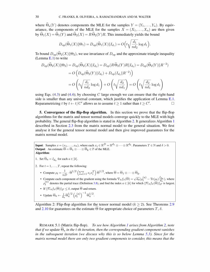
30 C. FRANKS, R. OLIVEIRA, A. RAMACHANDRAN AND M. WALTER
where Θa(Y ) denotes components the MLE for the samples Y = (Y1, . . . , Yn). By equiv-ariance, the components of the MLE for the samples X = (X1, . . . ,Xn) are then givenby Θ1(X) = Θ1(Y ) and Θ2(X) =R Θ2(Y )R. This immediately yields the bound
Dop(Θ1(X)‖Θ1) =Dop(Θ1(X)‖Id1) =O(t
√d1
nd2logd1
).
To bound Dop(Θ2(X)‖Θ2), we use invariance of Dop and the approximate triangle inequality(Lemma E.1) to write
Dop(Θ2(X)‖Θ2) =Dop(Θ2(X)‖Id2) =Dop(R Θ2(Y )R‖Id2) =Dop(Θ2(Y )‖R−2)
=O(Dop(Θ2(Y )‖Id2) +Dop(Id2‖R−2)
)=O
(t
√d1
nd2logd1
)+O
(t
√d2
nd1
)=O
(t
√d2
nd1logd1
)using Eqs. (4.3) and (4.4); by choosing C large enough we can ensure that the right-handside is smaller than any universal constant, which justifies the application of Lemma E.1.Reparametrizing t by t← t/C ′ allows us to assume t≥ 1 rather than t≥C ′.
5. Convergence of the flip-flop algorithm. In this section we prove that the flip-flopalgorithms for the matrix and tensor normal models converge quickly to the MLE with highprobability. The general flip-flop algorithm is stated in Algorithm 2. It generalizes Algorithm 1described in Section 2.3 from the matrix normal model to the general situation. We firstanalyse it for the general tensor normal model and then give improved guarantees for thematrix normal model.
Input: Samples x= (x1, . . . , xn), where each xi ∈RD = Rd1 ⊗ · · · ⊗Rdk . Parameters T ∈N and δ > 0.Output: An estimate Θ = Θ1 ⊗ · · · ⊗Θk ∈ P of the MLE.Algorithm:
1. Set Θa = Ida for each a ∈ [k].
2. For t= 1, . . . , T , repeat the following:
• Compute ρt =1
nD·Θ1/2
(∑ni=1 xix
Ti
)Θ
1/2, where Θ = Θ1 ⊗ · · · ⊗Θk .
• Compute each component of the gradient using the formula ∇afx(Θ) =√da(ρ
(a)t −Tr(ρt)
Idada
), whereρ
(a)t denotes the partial trace (Definition 3.8), and find the index a ∈ [k] for which ‖∇afx(Θ)‖F is largest.
• If ‖∇afx(Θ)‖F ≤ δ, output Θ and return.
• Update Θa← 1da
Θ1/2a
(ρ
(a)t
)−1Θ
1/2a .
Algorithm 2: Flip-flop algorithm for the tensor normal model (k ≥ 2). See Theorems 2.9and 2.10 for guarantees on the estimate Θ for appropriate choice of parameters T , δ.
REMARK 5.1 (Matrix flip-flop). To see how Algorithm 1 arises from Algorithm 2, notethat if we update Θa in the t-th iteration, then the corresponding gradient component vanishesin the subsequent iteration (we discuss why this is so below Lemma 5.3). Since for thematrix normal model there are only two gradient components to consider, this means that the
NEAR OPTIMAL SAMPLE COMPLEXITY FOR MATRIX AND TENSOR NORMAL MODELS 31
algorithm will necessarily alternate between updating Θ1 and Θ2. In other words, for thematrix normal model the algorithm truly “flip-flops” between the two coordinates.
Moreover, the same lemma shows that Trρt = 1 from the second iteration of Algorithm 2onwards. Using Lemma 3.9, and taking Υ as defined in Algorithm 1, it follows that
DF(Υ‖Θ−1a ) = ‖Ida −Θ
1/2a ΥΘ
1/2a ‖F = da‖
1
daΘ
1/2a ΥΘ
1/2a − Ida
da‖F
= da‖ρ(a)t −
Idada‖F =
√da‖∇afx(Θ)‖F .
Therefore, Algorithm 1 agrees with Algorithm 2 except that in the first iteration we skip thestopping condition and always update Θ1. This will not impact the analysis; see the proof ofLemma 5.6.
Before we analyze its convergence (for suitable choices of the parameters T and δ), wediscuss straightforward generalizations of standard convergence results for descent methodsunder strong convexity to the geodesically convex setting.
The next lemma shows that any descent method which manages to decrease the value ofthe function with respect to the gradient by a constant (more precisely the parameter α), ifstarting from a sublevel set where the function is strongly convex, will converge quickly to theoptimum. The proof of the lemma is a straightforward translation of a corresponding proof inFranks and Moitra (2020); we give it here for completeness.
LEMMA 5.2 (Proof of Lemma 4.11 in Franks and Moitra (2020)). Let f : P→ R beλ-strongly geodesically convex on a sublevel set S. Let x0 ∈ S and let α,β > 0 such that‖∇f(x0)‖2F ≤ β and xtt∈[T ] be a sequence satisfying
f(xt)≤ f(xt−1)− α ·minβ, ‖∇f(xt−1)‖2F
,(5.1)
for t ∈ [T ]. Then,
min0≤t≤T
‖∇f(xt)‖2F ≤ ‖∇f(x0)‖2F · 2−Tαλ.
PROOF. Let f∗ be the minimum value of the function f . Since f is λ-strongly geodesicallyconvex on S, we have
f∗ ≥ f(x)− 1
2λ‖∇f(x)‖2F(5.2)
for any x ∈ S. Since xt is a descent sequence, i.e., f(xt) ≤ f(xt−1) for all t ∈ [T ], weknow that each xt ∈ S. Therefore, Eq. (5.2) holds for any xt, 0≤ t≤ T .
We claim that for any xt such that ε := ‖∇f(xt)‖2F ≤ β, there exists `≤ 1/αλ such that‖∇f(xt+`)‖2F ≤ ε/2. This is enough to conclude the proof of the lemma, as with this claimwe see that we halve the squared norm of the gradient at every sequence of 1/αλ steps.
To prove the claim, we assume that ‖∇f(xt+`)‖2F ≥ ε/2 for all ` ∈ [m] (this is also truefor `= 0). We wish to show that m≤ 1/αλ. To see this, note that from Eq. (5.1) we have
f(xt+`)≤ f(xt+`−1)− α ·minβ, ‖∇f(xt+`−1)‖2F
≤ f(xt+`−1)− αε
2
for all ` ∈ [m], and therefore
f(xt+m)≤ f(xt)−αεm
2.
32 C. FRANKS, R. OLIVEIRA, A. RAMACHANDRAN AND M. WALTER
On the other hand, Eq. (5.2) implies that
f(xt+m)≥ f∗ ≥ f(xt)−1
2λ‖∇f(xt)‖2F ≥ f(xt)−
ε
2λ.
Together, we find that m≤ 1/αλ as claimed. This concludes our proof.
We now consider the flip-flop algorithm in Algorithm 2. Note that at the end of eachiteration, we update only a single Kronecker factor Θa. This update has the following property.
LEMMA 5.3 (Flip-flop update). Let t ∈ 1, . . . , T − 1 and assume the flip-flop algorithmhas not terminated before the (t+ 1)-st iteration. Then ρ(a)
t+1 = Idada
, where a ∈ [k] denotes theindex chosen in the t-th iteration. As a consequence, Trρt = 1 for t= 2, . . . , T .
In view of Lemma 3.9 and Remark 3.10, the above means that in each iteration but thefirst, ∇0fx(Θ) = 0 as well as ∇afx(Θ) = 0 for the a ∈ [k] chosen in the preceding iteration.Thus the flip-flop algorithm can be understood as carrying out an alternating minimization orcoordinate descent of the objective function fx.
PROOF. Let Θ denote the precision matrix at the beginning of the t-th iteration. Then,
ρ(a)t+1 =
(1
daΘ
1/2a
(ρ
(a)t
)−1Θ
1/2a
)1/2
Θ−1/2a ρ
(a)t Θ
−1/2a
(1
daΘ
1/2a
(ρ
(a)t
)−1Θ
1/2a
)1/2
=1
da
(Θ
1/2a
(ρ
(a)t
)−1Θ
1/2a
)1/2(Θ
1/2a
(ρ
(a)t
)−1Θ
1/2a
)−1(Θ
1/2a
(ρ
(a)t
)−1Θ
1/2a
)1/2
=1
daIda .
We now show that the flip-flop algorithm produces a descent sequence as in Eq. (5.1).
LEMMA 5.4 (Descent). Let k ≥ 2 and t ∈ 2, . . . , T − 1. Assume that the flip-flopalgorithm has not terminated before the (t + 1)-st iteration. Let Θ
(t), Θ(t+1) denote the
precision matrices at the beginning of the t-th and the (t+ 1)-st iteration, respectively. Then,
fx(Θ(t+1)
)≤ fx(Θ(t)
)− 1
6(k− 1)min
k− 1
dmax,‖∇fx(Θ
(t))‖2F.
If Trρ1 = 1 then this estimate also holds for t= 1.
PROOF. Recall that
fx(Θ(t)
) = Trρt −1
Dlog detΘ
(t).
and similarly for fx(Θ(t+1)
). By Lemma 5.3, we have Trρt = Trρt+1 = 1. Moreover, bydefinition of the update step
1
Dlog detΘ
(t+1)=
1
Dlog detΘ
(t) − 1
dalog det
(daρ
(a)t
).
It follows that
fx(Θ(t+1)
) = fx(Θ(t)
) +1
dalog det
(daρ
(a)t
).
NEAR OPTIMAL SAMPLE COMPLEXITY FOR MATRIX AND TENSOR NORMAL MODELS 33
Lemma 5.1 in Garg et al. (2019) states that for any d× d positive semidefinite matrix Z oftrace d, the following inequality holds:
log det(Z)≤−1
6min
‖Z − Id‖2F ,1
.
Applying this with Z = daρ(a)t , we obtain
1
dalog det
(daρ
(a)t
)≤−1
6min
‖ρ(a)
t −Idada‖2F ,
1
da
≤−1
6min
‖∇afx(Θ
(t))‖2F ,
1
da
≤−1
6min
‖∇fx(Θ
(t))‖2F
k− 1,
1
dmax
.
The equality follows from Lemma 3.9 and Remark 3.10. In the last inequality we used that∇0f(Θ
(t)) = 0 and at least one other component of the gradient is zero, as follows from
Lemma 5.3, and that a ∈ [k] is the index where the gradient has largest norm.
To prove that flip-flop converges once the initial conditions are satisfied, we need thefollowing general lemma on strongly geodesically convex functions, which tells us that oncethe gradient is small then the point must be inside a sublevel set of our function which iscontained in a ball where our function is strongly convex. This result is stated in Franks andMoitra (2020) for the manifold of positive definite matrices of determinant one, but the proofuses no specific properties of this manifold beyond the fact that it is a Hadamard manifold.Thus it holds for the manifold P as well.
LEMMA 5.5 (Proof of Lemma 4.7 in Franks and Moitra (2020)). Let f : P→ R be ageodesically convex function with optimizer x ∈ P (i.e.∇f(x) = 0), and further assume that fis λ-strongly geodesically convex on the ball Br(x). If y ∈ P is such that ‖∇f(y)‖F < λr/8,then y is contained in a sublevel set S of f which in turn is contained in Br(x). In particular,f is λ-strongly geodesically convex on S.
Now we must show that the flip-flop algorithm reaches a point with small enough gradientrelatively quickly. This is given by the following lemma, which follows the analysis givenby Garg et al. (2019); Bürgisser et al. (2018):
LEMMA 5.6 (Flip-flop reduces gradient). For any γ > 0, Algorithm 2 reaches some Θsuch that ‖∇fx(Θ)‖F < γ within the first
T0 =
⌈3 + 6(k+ 1)
(1 + log fx(ID)− f∗x
)max
dmax
k− 1,
1
γ2
⌉iterations, where f∗x := infΘ∈P fx(Θ) (if it has not terminated earlier).
PROOF. We denote by Θ(t) the precision matrices at the beginning of the t-th iteration of
the flip-flop algorithm. We will analyze the flip-flop algorithm starting at Θ(1)
= 1fx(ID)ID
rather than ID , so that Trρ1 = 1, and skipping the stopping criterion in the first iteration. Notethat the iterates Θ
(t) for t= 2, . . . , T0 from this initialization agree with the iterates initializedat the identity. This is because multiplying ρ1 by a scalar leads to the same update at the endof the first flip-flop iteration, hence to the same Θ
(2).
34 C. FRANKS, R. OLIVEIRA, A. RAMACHANDRAN AND M. WALTER
By Lemma 5.4, using that Trρ1 = 1, we have that
f∗x ≤ fx(Θ(T0)
)≤ fx(Θ(1)
)− 1
6(k− 1)
T0−1∑t=2
min
k− 1
dmax,‖∇fx(Θ
(t))‖2F
(we omit the summand for t= 1). Therefore, if ‖∇fx(Θ(t)
)‖F ≥ γ for t= 2, . . . , T0− 1, then
T0 − 2
6(k− 1)min
k− 1
dmax, γ2
≤ fx(Θ
(1))− f∗x = 1 + log fx(ID)− f∗x
This implies the desired bound.
We now have all the tools we need to prove that, given appropriate initial conditions on thesamples (which we later show to hold when the samples are drawn from the tensor normalmodel with precision matrix Θ), the flip-flop algorithm will converge quickly to the MLE.Namely, we show that the MLE is in a constant size operator norm ball around the trueprecision matrix, where the negative log-likelihood is strongly geodesically convex. Thisimplies that the log-likelihood is strongly geodesically convex in a small geodesic ball aroundthe MLE. Hence, by Lemma 5.5, any point with sufficiently small gradient of the log-likelihoodfunction is contained in a sublevel set on which the log-likelihood is strongly geodesicallyconvex. By Lemma 5.6, such a point is found in polynomially many iterations of the flip-flopalgorithm, at which point Lemma 5.2 applies to yield an δ-minimizer in O(log(1/δ)) furtheriterations. To state our result, we use the metric dop(A,B) = ‖logB−1/2AB−1/2‖op definedin Eq. (3.17).
THEOREM 5.7 (Convergence from initial conditions). Let Θ ∈ P, x1, . . . , xn ∈ RD,and λ, ζ > 0 be such that
1. fx is λ-strongly geodesically convex at any Θ′ ∈ P such that dop(Θ′,Θ) ≤ ζ , whereζ ≤min1,16
√(k+ 1)(k− 1)/λ.
2. |∇0fx(Θ)| ≤ 1/2.3. The MLE Θ exists and satisfies dop(Θ,Θ)≤ ζ/2.
Then, for every 0< δ < λζ/16√
(k+ 1)dmax, Algorithm 2 within
T =
⌈3 + 1536
(1 + logκ(Θ)
)(k+ 1)2dmax
ζ2λ2
⌉+
⌈18(k− 1)
λlog
λζ
16√
(k+ 1)dmax · δ
⌉iterations outputs Θ with d(Θ, Θ)≤ δ
λ and DF(Θa‖Θa)≤ 2√da · δλ for all a ∈ [k].
PROOF. By the triangle inequality for dop, the first and the third assumptions imply that fxis λ-strongly geodesically convex at all Θ′ ∈ P such that dop(Θ′, Θ)≤ ζ/2. In particular, it isλ-strongly geodesically convex on the geodesic ball Br(Θ) of radius
r =ζ
2√
(k+ 1)dmax
by Remark 3.22.First note that our error bounds on the MLE follow if Algorithm 2 reaches the stopping
criterion within T iterations, that is, if we reach a precision matrix Θ = Θ(t) such that
‖∇fx(Θ)‖F ≤ δ. Indeed, since δ < λr8 by our assumption on δ, Lemma 5.5 applies (with x=
NEAR OPTIMAL SAMPLE COMPLEXITY FOR MATRIX AND TENSOR NORMAL MODELS 35
Θ, y = Θ) and shows that Θ ∈Br(Θ). Now Lemma 3.6 applies, since in particular r > 2δ/λ,and shows that Θ ∈Bδ/λ(Θ), i.e.,
d(Θ, Θ)≤ δ
λ
(up a factor 8, this already follows from Lemma 5.5). Finally, note that our assumption on δalso implies that δ ≤ λ/
√dmax. Thus we can apply Lemma 3.7 to obtain
DF(Θa‖Θa)≤ 2√da ·
δ
λ
for all a ∈ [k]. These are the desired error bounds on the MLE.It remains to argue that Algorithm 2 stops within T iterations. We start by reasoning about
the number of steps required before strong convexity applies. By Lemma 5.6 with γ = λr/8,within at most
T0 =
⌈3 + 6(k+ 1)
(1 + log fx(ID)− f∗x
)max
dmax
k− 1,
64
r2λ2
⌉(5.3)
iterations, where f∗x := fx(Θ), the algorithm reaches a point Θ(t0) such that
‖∇fx(Θ(t0)
)‖F <λr
8.
We can use Lemma 5.5 (with x= Θ, y = Θ(t0)) to see that Θ
(t0) is contained in a sublevel setof fx on which fx is λ-strongly geodesically convex.
Note also that ‖∇fx(Θ(t0)
)‖2F ≤ β := k−1dmax
because λr/8 = λζ/16√
(k+ 1)dmax ≤√(k− 1)/dmax by our assumption that ζ ≤ 16
√(k+ 1)(k− 1)/λ.
Therefore, Lemma 5.4 shows that each subsequent step of the algorithm will decreasethe value of the objective function in accordance with the requirements of Lemma 5.2, withparameters α= 1
6(k−1) and β as defined above. Thus, for any δ > 0, within at most
T1 :=
⌈6(k− 1)
λlog2
‖∇fx(Θ(t0)
)‖2Fδ2
⌉≤
⌈12(k− 1)
λlog2
‖∇fx(Θ(t0)
)‖Fδ
⌉
≤⌈
18(k− 1)
λlog
λr
8δ
⌉=
⌈18(k− 1)
λlog
λζ
16√
(k+ 1)dmax · δ
⌉
further iterations we will encounter a point Θ = Θ(t) such that ‖∇fx(Θ)‖F ≤ δ, i.e., such that
the algorithm will stop.Finally, we bound our expression for T0 in Eq. (5.3) using the assumptions. On the one
hand,
f∗x = fx(Θ) = Tr Θρ1 −1
Dlog det Θ = 1− 1
Dlog det
(Θ1/2Θ−1/2ΘΘ−1/2Θ1/2
)≥ 1− ζ
2− 1
Dlog det Θ≥ 1− ζ
2− log‖Θ‖op,
where the third equality follows since ∇0fx(Θ) = Tr Θρ1 − 1 = 0 at the MLE; the finalinequality holds because dop(Θ,Θ)≤ ζ/2 by our third assumption, hence Θ−1/2ΘΘ−1/2 eζ/2ID . On the other hand,
fx(ID) = Trρ1 = Tr Θ−1Θρ1 ≤ ‖Θ−1‖op Tr Θρ1 ≤3
2‖Θ−1‖op,
36 C. FRANKS, R. OLIVEIRA, A. RAMACHANDRAN AND M. WALTER
using the second assumption, which states that |∇0fx(Θ)|= |Tr Θρ1 − 1| ≤ 12 . Together,
log fx(ID)− f∗x ≤ log3
2+ log‖Θ−1‖op − 1 +
ζ
2+ log‖Θ‖op ≤ logκ(Θ),
using the assumption that ζ ≤ 1. Finally, we can simply the maximum in Eq. (5.3) using againthat λr/8 = λζ/16
√(k+ 1)dmax ≤
√(k− 1)/dmax. We obtain
T0 ≤⌈
3 + 6(k+ 1)(1 + logκ(Θ)
) 64
r2λ2
⌉=
⌈3 + 1536
(1 + logκ(Θ)
)(k+ 1)2dmax
ζ2λ2
⌉.
Adding the bound on T1 concludes the proof.
5.1. Proofs of Theorem 2.9 and 2.10. We are now ready to prove the fast convergence ofthe flip-flop algorithm to the MLE.
THEOREM 2.9 (Tensor flip-flop convergence, restated). There are universal con-stants C,c > 0 such that the following holds. Suppose x= (x1, . . . , xn) are n≥Ck2d3
max/Dindependent samples from the tensor normal model with precision matrix Θ = Θ1 ⊗ · · · ⊗Θk .Then, with probability at least
1− k e−Ω( nD
k2d2max) − k2
(√nD
kdmax
)−Ω(dmin)
,
the MLE Θ exists, and for every 0< δ < c/√
(k+ 1)dmax, Algorithm 2 within
T =O
(k2dmax
(1 + logκ(Θ)
)+ k log
1
δ
)iterations outputs Θ with d(Θ, Θ)≤ 2δ and DF(Θa‖Θa)≤ 4
√da · δ for all a ∈ [k].
PROOF. For λ= 12 , r = ζ/
√(k+ 1)dmax, and ζ a universal constant, consider the follow-
ing two events:
1. fx is λ-strongly geodesically convex at any Θ′ ∈ P such that dop(Θ′,Θ) ≤ ζ , whereζ ≤min1,16
√(k+ 1)(k− 1)/λ. In particular, fx is λ-strongly geodesically convex on
the geodesic ball Br(Θ).2. ‖∇fx(Θ)‖F < rλ
2 . In particular, |∇0fx(Θ)|< 12 .
We first bound the success probability of these events similarly to the proof of Proposition 3.23.For this, we may assume without loss of generality that Θ = ID by Remarks 3.10 and 3.15.Then the first event holds with probability at least 1− k2(
√nD
kdmax)−Ω(dmin) by Proposition 3.21
and Remark 3.22, provided we choose C large enough and ζ small enough. For the secondevent, we apply Proposition 3.11 with
ε=1
10√k
rλ
2=
ζ
40√k(k+ 1)dmax
,
which satisfies ε < 1 and n≥ d2max
Dε2 provided we choose ζ sufficiently small and C sufficientlylarge. We find that the second event holds with probability at least
1− 2(k+ 1)e−ε2 nD
8dmax = 1− k e−Ω( nD
k2d2max).
Thus, the two events hold simultaneously with the desired success probability by the unionbound. Moreover, by Lemma 3.6, the two events together also imply the following:
NEAR OPTIMAL SAMPLE COMPLEXITY FOR MATRIX AND TENSOR NORMAL MODELS 37
3. The MLE Θ exists and satisfies d(Θ,Θ)≤ r/2. In particular, dop(Θ,Θ)≤ ζ/2.
Accordingly, the theorem follows from Theorem 5.7, noting that
T =
⌈3 + 1536
(1 + logκ(Θ)
)(k+ 1)2dmax
ζ2λ2
⌉+
⌈18(k− 1)
λlog
λζ
16√
(k+ 1)dmax · δ
⌉
=O
(k2dmax
(1 + logκ(Θ)
)+ k log
1
δ
)and taking c= λζ/16 = ζ/32.
We now give an improved analysis for the matrix flip-flop algorithm with exponentiallysmall failure probability under the hypotheses of Theorem 2.7.
THEOREM 2.10 (Matrix flip-flop convergence, restated). There are universal con-stants C,c > 0 such that the following holds. Let 1< d1 ≤ d2. Suppose x1, . . . , xn ∈ Rd1d2are
n≥Cd2
d1max
logd2, log2 d1
independent samples from the matrix normal model with precision matrix Θ = Θ1⊗Θ2. Then,with probability at least 1−e−Ω(nd21/d2 log2 d1), the MLE Θ exists, and for every 0< δ < c/
√d2,
Algorithms 1 and 2 within
T =O
(d2
(1 + logκ(Θ)
)+ log
1
δ
)iterations outputs Θ with d(Θ, Θ) =O(δ) and DF(Θa‖Θa) =O(
√da · δ) for all a ∈ 1,2.
PROOF. Consider the following three events for universal constants λ, ζ > 0:
1. fx is λ-strongly geodesically convex at any Θ′ ∈ P such that dop(Θ′,Θ) ≤ ζ , whereζ ≤min1,16
√3/λ.
2. |∇0fx(Θ)| ≤ 1/2.3. The MLE Θ exists and satisfies dop(Θ,Θ)≤ ζ/2.
We first bound the success probability of these events. For this, we may assume without loss ofgenerality that Θ = ID by Remarks 3.10 and 3.15. Then, if λ ∈ (0,1) is a suitable constant, Cis large enough, and ζ is small enough, then by Corollary 4.6 with t2 = nd1/d2, the first eventholds with probability at least 1− e−Ω(nd1) ≥ 1− e−Ω(nd21/d2 log2 d1) in view of our assumptionon n.
The second event holds with probability at least 1 − e−Ω(nD) by Proposition 3.13. Fi-nally, by Theorem 2.7 with t2 = nd1/d2 log2 d1 (which can be made larger than 1 by ourassumption on n assuming C is large enough), the third event holds with probability atleast 1− e−Ω(nd21/d2 log2 d1). To obtain the second event from Theorem 2.7 we use Lemma E.3to relate Dop to dop and that dop(Θ1⊗ Θ2,Θ1⊗Θ2)≤ dop(Θ1,Θ1) +dop(Θ2,Θ2). Thus, allthree events hold simultaneously with probability at least 1− e−Ω(nd21/d2 log2 d1) by the unionbound. Accordingly, the theorem follows from Theorem 5.7 with k = 2, noting that
T =
⌈3 + 1536
(1 + logκ(Θ)
)(k+ 1)2dmax
ζ2λ2
⌉+
⌈18(k− 1)
λlog
λζ
16√
(k+ 1)dmax · δ
⌉
38 C. FRANKS, R. OLIVEIRA, A. RAMACHANDRAN AND M. WALTER
=
⌈3 + 13824
(1 + logκ(Θ)
) d2
ζ2λ2
⌉+
⌈18
λlog
λζ
16√
3d2 · δ
⌉=O
(d2
(1 + logκ(Θ)
)+ log
1
δ
)and taking c= λζ/16
√3.
6. Lower bounds. In this section we discuss known lower bounds for estimating unstruc-tured precision matrices (i.e., the case k = 1 of the tensor normal model). Afterwards weprove a new lower bound on the matrix normal model.
6.1. Lower bounds for unstructured precision matrices. Here we briefly recall and, forcompleteness, prove well-known lower bounds on the accuracy of any estimator for theprecision matrix in the Frobenius and operator error from independent samples of a Gaussian.The lower bounds follow from Fano’s method and the relationship between the Frobeniuserror and the relative entropy (which is proportional to Stein’s loss). Informally, both boundsimply that no estimator for a d× d precision matrix from n samples can have accuracy smallerthan d/
√n (resp.
√d/n) in Frobenius error or relative Frobenius error (resp. operator norm
error or relative operator norm error) with probability more than 1/2.
PROPOSITION 6.1 (Frobenius and operator error). There is c > 0 such that the followingholds. Let X ∈Rd×n denote n independent random samples from a Gaussian with precisionmatrix Θ ∈ PD(d). Consider any estimator Θ = Θ(x) for the precision matrix Θ, and letB ⊂ PD(d) denote the ball about Id of radius 1/2 in the operator norm.
1. Let δ2 = c min
1, d2/n
. Then,
supΘ∈B
Pr[‖Θ−Θ‖F ≥ δ
]≥ 1
2.(6.1)
2. Let δ2 = c min1, d/n. Then,
supΘ∈B
Pr[‖Θ−Θ‖op ≥ δ
]≥ 1
2.(6.2)
As a consequence, we have
supΘ∈B
E[‖Θ−Θ‖2F ] = Ω
(min
d2
n,1
)and sup
Θ∈BE[‖Θ−Θ‖2op] = Ω
(min
d
n,1
).
The proof uses Fano’s inequality with mutual information bounded by relative entropy, asin Yang and Barron (1999).
LEMMA 6.2 (Fano’s inequality). Let Pii∈[m] be a finite set of probability distributionsover a set X , and let T :X → [m] be an estimator for i from a sample of Pi. Then
maxi∈[m]
PrX∼Pi
[T (X) 6= i]≥ 1−log 2 + maxi,j∈[m]DKL(Pi‖Pj)
logm.
PROOF OF PROPOSITION 6.1. We first prove Eq. (6.1), the lower bound on estimation inthe Frobenius norm. We begin by the standard reduction from estimation to testing. Let V0 bea 1-separated set in the Frobenius ball BF of radius 1 in the d× d symmetric matrices, i.e.,the set BF = A :A Symmetric,‖A‖F ≤ 1.
NEAR OPTIMAL SAMPLE COMPLEXITY FOR MATRIX AND TENSOR NORMAL MODELS 39
We may take V0 to have cardinality m≥ 2d(d+1)/2 because BF is a Euclidean ball of radius1 in the linear subspace of d× d symmetric matrices, which has dimension d(d+ 1)/2, andhence any maximal Frobenius 1/2-packing (collection of disjoint radius 1/2 Frobenius balls)in BF has cardinality at least 2d(d+1)/2. Let 0≤ δ ≤ 1/2, and let V = Id + δV0 = Id + δv :v ∈ V0. Write V = Θ1, . . . ,Θm. Note that V is contained within the operator norm ball B.Let Pi =N (0,Θ−1
i )⊗n for i ∈ [m], and define the estimator T by
T (x) = arg mini∈[m]
‖Θi − Θ(x)‖F .
Then, because V is 2δ-separated,
PrX∼Pi
[T (X) = i]≥ Pr[‖Θ−Θi‖F ≤ δ
].(6.3)
In order to apply Fano’s inequality, we use the well-known fact that DKL(Pi‖Pj) =nDKL(N (0,Θ−1
i ) ‖ N (0,Θ−1j )) = O(nDF(Θj ‖ Θi)
2) when Θ−1i Θj has eigenvalues uni-
formly bounded away from zero by the proof of Lemma E.2. This condition on the eigenvaluesholds because Id/2Θj ,Θj 3Id/2 for i, j ∈ [m] by our assumption that δ ≤ 1/4.
Moreover, for i ∈ [m], we have ‖Θ−1i ‖op ≤ 2 and so DF(Θj‖Θi) = O(‖Θi −Θj‖F ) =
O(δ) by Eq. (E.1). Thus we have DKL(Pi‖Pj)≤Cnδ2 for some absolute constant C . Then,by Lemma 6.2,
mini∈[m]
PrX∼Pi
[T (X) = i]≤ log 2 +Cnδ2
d(d+ 1)(log 2)/2.
If δ2 = c mind2n ,1, the right-hand side of the inequality above is bounded by 12 and the
assumption δ ≤ 1/4 is satisfied provided c is a small enough absolute constant. In view ofEq. (6.3), it follows that
mini∈[m]
Pr[‖Θ−Θi‖F ≤ δ
]≤ 1/2.
Because V ⊂B, this proves Eq. (6.1).To obtain Eq. (6.2), the lower bound in operator norm, instead start with a packing V0 of the
unit operator norm ball of cardinality m≥ 2d(d+1)/2 and define V = Θ1, . . . ,Θm as above.We modify the proof by bounding DKL(Pi‖Pj) =O(n‖Θi−Θj‖2F ) =O(nd‖Θi−Θj‖2op)≤Cndδ2. Proceeding as before, we find that for δ = c min dn ,1,
mini∈[m]
Pr[‖Θ−Θi‖op ≤ δ
]≤ 1/2.
Again, we have V ⊂B, so Eq. (6.2) follows.
We remark that the above proof shows the necessity of a scale-invariant dissimilaritymeasure to obtain error bounds that are independent of the ground truth precision matrix Θ.Indeed, replacing the packing V by κV for κ→∞ in the proof shows that supΘ∈κB Pr[‖Θ−Θ‖F ≥ κδ]≥ 1
2 . That is, no fixed bound can be obtained with probability 1/2.We now use the result just obtained to prove bounds on the relative Frobenius and operator
error. Because Id/2Θ 3Id/2 for Θ ∈B, the bounds ‖Θ− Θ‖F ≤ ‖Θ‖opDF(Θ‖Θ) and‖Θ− Θ‖op ≤ ‖Θ‖opDop(Θ‖Θ) together with Proposition 6.1 imply the following corollary.
COROLLARY 6.3 (Relative Frobenius and operator error). There is c > 0 such that thefollowing holds for X, Θ,B as in Proposition 6.1.
40 C. FRANKS, R. OLIVEIRA, A. RAMACHANDRAN AND M. WALTER
1. Let δ2 = c min
1, d2/n
. Then
supΘ∈B
Pr[DF(Θ‖Θ)≥ δ
]≥ 1
2.(6.4)
2. Let δ2 = c min1, d/n. Then
supΘ∈B
Pr[Dop(Θ‖Θ)≥ δ
]≥ 1
2.(6.5)
As a consequence, we have
supΘ∈B
E[DF(Θ‖Θ)2] = Ω
(min
d2
n,1
)and sup
Θ∈BE[Dop(Θ‖Θ)2] = Ω
(min
d
n,1
).
6.2. Lower bounds for the matrix normal model. If Θ2 is known, then we can compute(I ⊗Θ
1/22 )X , which is distributed as nd2 independent samples from a Gaussian with preci-
sion matrix Θ1. In this case, one can estimate Θ1 in operator norm with an RMSE rate ofO(√d1/nd2). One could hope that this rate holds for Θ1 even when Θ2 is not known. Here
we show that, to the contrary, the rate for Θ1 cannot be better than O(√d1/nmin(nd1, d2)).
Thus, for d2 > nd1, it is impossible to estimate Θ1 as well as one could if Θ2 were known.Note that, in this regime, there is no hope of recovering Θ2 even if Θ1 is known.
THEOREM 6.4 (Lower bound for matrix normal models). There is c > 0 such that thefollowing holds. Let Θ1 be any estimator for Θ1 from a tuple X of n samples of the matrixnormal model with precision matrices Θ1,Θ2. Let B ⊂ PD(d1) denote the ball about Id1 ofradius 1/2 in the operator norm.
1. Let δ2 = c min
1, d21nminnd1,d2
. Then
supΘ1∈B,Θ2∈PD(d2)
Pr[DF(Θ1‖Θ1)≥ δ
]≥ 1
2.(6.6)
2. Let δ2 = c min
1, d1nminnd1,d2
. Then
supΘ1∈B,Θ2∈PD(d2)
Pr[Dop(Θ1‖Θ1)≥ δ
]≥ 1
2.(6.7)
As a consequence, we have
supΘ1∈B,Θ2∈PD(d2)
E[DF(Θ1‖Θ1)2] = Ω
(min
d2
1
nminnd1, d2,1
)
and supΘ1∈B,Θ2∈PD(d2)
E[Dop(Θ1‖Θ1)2] = Ω
(min
d1
nminnd1, d2,1
).
Intuitively, the above theorem holds because we can choose Σ2 to zero out all but nd1
columns of each Xi, which allows access to at most n · nd1 samples from a Gaussian withprecision Θ1. However, this does not quite work because Σ2 would not be invertible and hencethe precision matrix Θ2 would not exist. We must instead choose Σ2 to be approximatelyequal to a random projection of rank nd1. The resulting construction allows us to deducethe same lower bounds for estimating Θ1 as the Gaussian case with at most nmind2, nd1independent samples.
NEAR OPTIMAL SAMPLE COMPLEXITY FOR MATRIX AND TENSOR NORMAL MODELS 41
One might ask why the rank of the random projection cannot be taken to be even less thannd1, yielding an even stronger bound. If the rank is less than nd1, then the support of Σ2 canbe estimated. This would allow one to approximately diagonalize Σ2 so that the n samples canbe treated as nd2 independent samples in Rd1 , yielding the rate
√d1/nd2 using, e.g., Tyler’s
M estimator. We now state the lower bound.
LEMMA 6.5. Let X denote a tuple of n samples from the matrix normal model with preci-sion matrices Θ1,Θ2. Let Y be a tuple of nminnd1, d2 Gaussians on Rd1 with precisionmatrix Θ1. Let Θ1(X) be any estimator for Θ1. For every δ > 0, there is a distribution onΘ2 and an estimator Θ(Y ) such that the distribution of Θ1(X) and the distribution of Θ(Y )differ by at most δ in total variation distance.
PROOF. If d2 ≤ nd1, then setting Θ2 = Id2 shows that Θ1 has access to precisely nd2
samples from a Gaussian Rd1 with precision matrix Θ1. Thus we may take Θ = Θ1 in thatcase, completing the proof. The harder case is d2 > nd1.
For intuition, let B be any d2 × d2 matrix such that the last d2 − nd1 columns are zero.Given access to the tuple X of n samples
√Σ1ZiB
T , where Zi are i.i.d standard Gaussiand1 × d2 matrices, clearly Θ2 has access to at most n2d1 samples of the Gaussian on Rd1 withprecision matrix Θ1 because ZiBT depends only on the first d1 columns of each Zi.
However, we must supply invertible B in order for Θ2 = (BBT )−1 to exist. Let δ ≥ 0.Let Bδ be the random matrix obtained by choosing the first nd1 columns of Bδ uniformly atrandom among the collections of nd1 orthonormal vectors in Rd2 . Let the remaining entriesbe i.i.d uniform in [−δ, δ] (the precise distribution of the remaining entries does not matter aslong as they are independent, continuous, and small). Let Yδ := (
√Σ1Z1B
Tδ , . . . ,
√Σ1ZnB
Tδ )
denote the resulting random variable with Bδ and X chosen independently. If δ = 0, then, bythe argument above, with access to the random variable Yδ := (
√Σ1Z1B
Tδ , . . . ,
√Σ1ZnB
Tδ )
the estimator Θ1 has access to at most n2d1 samples of a Gaussian on Rd1 with precisionmatrix Θ1. We claim that as δ→ 0, the distribution of Yδ tends to that of Y0 in total variationdistance. Thus the distribution of Θ1(Yδ) converges to that of Θ1(Y0) in total variation. SinceY0 only depends on n2d1 samples to the Gaussian on Rd1 with precision matrix Θ1, whichwe call Y , defining Θ(Y ) = Θ1(Y0) proves the theorem. 1
It remains to prove that Yδ converges to Y0 in total variation distance. First note thatYδ = Y0 + δW where Wi =
√Θ1ZiC
T , where C is a random matrix where the first nd1
columns are zero and the last d2− nd1 columns have entries i.i.d uniform on [−1,1]. Becauseof the zero patterns of B0 and C and the fact that the entries of Z are i.i.d., the randomvariables Y0 and W are independent. If we can show that Y0 has a density with respect to theLebesgue measure on Rnd1d2 , then Y0 + δW converges to Y0 in total variation distance asδ→ 0. This follows because Y0 + δW has a density obtained by convolving the density of Y0,an L1 function, by the law of δW . The density of Y0 + δW then converges to that of Y0 in L1
by the continuity of the translation operator in L1.2
By invertibility of Σ1, it is enough to show that Y0 has a density when Σ1 = Id1 . ConsiderY0 = (Z1B
T0 , . . . ,ZnB
T0 ). We may think of Y0 as the d2 × nd1 random matrix obtained by
horizontally concatenating the matrices B0ZTi . 3
1Actually, as B has a probability zero chance of being singular, the final family of densities Y ′δ we will use isYδ conditioned on B being invertible. As B is invertible with probability 1 for δ > 0, the total variation distancebetween Y ′δ , Yδ is zero for all δ > 0 and hence Y ′δ converges to Y0 in total variation distance provided Yδ does.
2We thank Oliver Diaz for communicating a proof of this fact.3Almost every matrix of these dimensions has rank nd1, but if we had set even more of the columns of B0 to
zero then Y0 would have rank less than nd1 with probability 1 and hence would not have a density. This is why wecannot push this argument any further.
42 C. FRANKS, R. OLIVEIRA, A. RAMACHANDRAN AND M. WALTER
Now consider the nd1 random vectors in Rd2 that are the columns of the matrices B0ZTi ,
for i ∈ 1, . . . , n. Because B0 is supported only in its first nd1 columns, the joint distributionof these random vectors may be obtained by sampling nd1 independent standard Gaussianvectors vj on Rnd1 and then multiplying them by the d2×nd1 matrix B′ that is the restrictionof B0 to its first nd1 columns. We have chosen B′ such that it is an isometry into a uniformlyrandom subspace of Rd2 of dimension nd1. Thus Bvj/‖vj‖ are nd1 many independent,random unit vectors in Rd2 . As the ‖vj‖ are also independent, Bvj are thus independent. Eachmarginal Bvi has a density; one may sample it by choosing a uniformly random vector andthen choosing the length ‖vi‖, hence the density is a product density in spherical coordinates.The joint density of the Bvj is then the product density of the marginal densities.
The above lemma combined with Corollary 6.3 immediately implies Theorem 6.4. Weremark that the below proof uses no properties about DF; a lower bound on any error metricfor estimating a Gaussian with nminnd1, d2 samples will transfer to the matrix normalmodel. In particular, Theorem 6.4 holds true when DF is replaced by the Frobenius error andDop replaced by the operator norm error.
PROOF OF THEOREM 6.4. To show Item 1, let δ2 ≤ c min
1, d21nminnd1,d2
. Let Θ2 be
the distributed as in Lemma 6.5 so that, as guaranteed by Lemma 6.5 there is an estimatorΘ with access to a tuple Y of nminnd1, d2 samples of a Gaussian on Rd1 with precisionmatrix Θ1 satisfyingDTV(Θ1(X), Θ(Y ))≤ δ0. HereX is distributed according to the normalmodel with precision matrices Θ1,Θ2. Corollary 6.3 implies
supΘ∈B
PrY
[DF(Θ(Y )‖Θ1)≥ δ
]≥ 1
2.
Clearly we have
supΘ1∈B,Θ2∈PD(d2)
PrX
[DF(Θ1(X)‖Θ1)≥ δ
]≥ sup
Θ1∈BPr
Θ2,X
[DF(Θ1(X)‖Θ1)≥ δ
].
On the other hand, the total variation distance bound implies
supΘ1∈B
PrΘ2,X
[DF(Θ1(X)‖Θ1)≥ δ
]≥ sup
Θ1∈BPrY
[DF(Θ(Y )‖Θ1)− δ0 ≥ δ
]≥ 1
2− δ0.
Allowing δ0→ 0 implies the theorem. The proof of Item 2 is the same but with DF replacedby Dop.
7. Numerics and regularization. In the undersampled regime, most effort so far hasfocused on the sparse case. Existing estimators, such as the Gemini estimator Zhou (2014)and KGlasso estimator Tsiligkaridis, Hero and Zhou (2013) enforce sparsity by adding aregularizer proportional to the `1 norm of the precision matrices to encourage sparsity. We referto these as Glasso-type estimators. We propose a new, shrinkage-based estimator that is simpleto compute and experimentally outperforms Gemini and KGlasso in a natural generativemodel.
To describe our estimator, we remind the reader that the maximum likelihood estimatoras defined in Eq. (3.5) is the optimum of a function depending on the sample covariancematrix. Namely, we choose Θ ∈ P optimizing Tr Θρ− 1
D log det Θ where ρ= 1nD
∑ni=1 xix
Ti
NEAR OPTIMAL SAMPLE COMPLEXITY FOR MATRIX AND TENSOR NORMAL MODELS 43
is the sample covariance matrix.4 In our estimator, ρ is replaced by a shrinkage estimator forthe covariance matrix. Namely, we replace ρ by ρ := (1− α)ρ+ αTrρ
D I for some α ∈ [0,1].Formally, define Θα
x = arg minΘ∈P fαx (Θ) where
fαx (Θ) := Tr Θ
((1− α)ρ+ α
Trρ
DI
)− 1
Dlog det Θ.
This is known as a shrinkage estimator with ridge regularization (Warton, 2008). Theestimator, which we call the shrinkage-based flip-flop estimator, or ShrinkFlop for short, isclosely related to the shrinkage estimator considered in Goes et al. (2020) and the Frobeniuspenalty considered in Tang and Allen (2018).
We consider a generative model in which the covariance matrices Θi are distributed as arank one Wishart matrix plus a small multiple of the identity matrix to ensure invertibility;we refer to them as spiked covariance matrices. We also show that, even when Θ1 is sparse,our shrinkage-based estimator can outputerform Gemini and KGlasso when Σ2 is spiked.Moreover, we observe that our regularized estimator is significantly faster to compute than theGlasso-type estimators. All three estimators require parameter tuning, so when possible wecompare throughout a plausible range of parameters for each of them. We leave determinationof α by cross-validation for future work.
7.1. ShrinkFlop estimator. We now discuss some properties of the ShrinkFlop estimator.As above, set ρ := (1− α)ρ+ αTrρ
D I. If α > 0, then ρ is invertible and therefore Θαx exists
uniquely for every x. This is because, whenever ρ is invertible, the function fαx is strictlygeodesically convex even on the larger domain PD(D) (see Example 3.4). Thus it has aunique minimizer over the geodesically convex domain P.
The estimator Θαx can be approximately computed using the flip-flop algorithm (as in
Algorithm 2) with ρ replaced by ρ. Due to the special form of ρ, one need not look atthe entirety of ρ to perform each step of the flip-flop algorithm. The resulting algorithm issummarized in Algorithm 3. The only modification as compared to the original algorithm isthat at each flip-flop step the estimate of the covariance is replaced by a convex combinationwith a scaled identity matrix, as well as the computation of the gradient.
7.2. Scenario 1: Spiked, dense covariances. Here we compare the performance of ourshrinkage based estimator with Zhou’s single step estimator (Gemini) for the matrix normalmodel assuming Σ1,Σ2 are dense, spiked covariance matrices. Fig. 1 was generated by settingd1 = 25, d2 = 50 and n= 1, and for each choice of regularization parameter independentlygenerating 5 different pairs Σ1 ∼ Id1 + 10v1v
T1 and Σ2 ∼ Id2 + 10v2v
T2 where the vi are stan-
dard di-dimensional Gaussian vectors and then normalizing each to have trace di, respectively.As in Zhou (2014), we always normalize the trace of Θ1 to match that of Θ1 to focus onthe core difficulties rather than estimating the overall scale of the data (which is easy to do).Though our main focus is estimation in geodesic distance, we also considered the Frobeniusdistance due to its prevalence in the literature. For each of the 5 pairs, following Tsiligkaridis,Hero and Zhou (2013) we computed the normalized squared error (the squared Frobeniusdistance from Θ1 to Θ1 divided by the squared Frobenius norm of Θ1 for samples drawn fromthis distribution 5 times. Finally we averaged all 25 errors. Note that with d1 = 25, d2 = 50and n= 1, the MLE never exists and so we cannot compare with flip-flop without shrinkage.
We also computed the error in geodesic distance. We used geodesic distance in place ofthe relative Frobenius error (Definition 2.3) because these quantities are comparable (see
4or, more accurately, the matrix of second moments
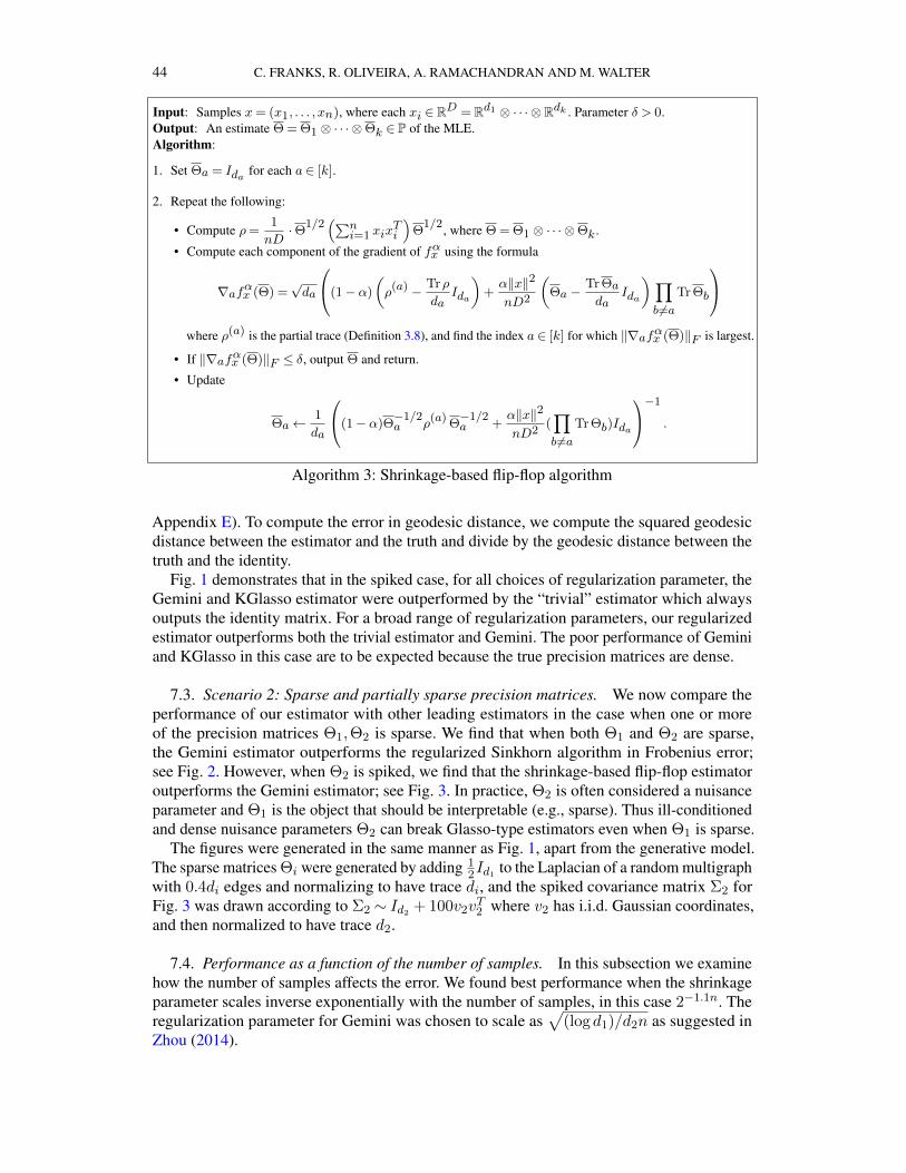
44 C. FRANKS, R. OLIVEIRA, A. RAMACHANDRAN AND M. WALTER
Input: Samples x= (x1, . . . , xn), where each xi ∈RD = Rd1 ⊗ · · · ⊗Rdk . Parameter δ > 0.Output: An estimate Θ = Θ1 ⊗ · · · ⊗Θk ∈ P of the MLE.Algorithm:
1. Set Θa = Ida for each a ∈ [k].
2. Repeat the following:
• Compute ρ=1
nD·Θ1/2
(∑ni=1 xix
Ti
)Θ
1/2, where Θ = Θ1 ⊗ · · · ⊗Θk .
• Compute each component of the gradient of fαx using the formula
∇afαx (Θ) =√da
(1− α)
(ρ(a) − Trρ
daIda
)+α‖x‖2
nD2
(Θa −
Tr Θada
Ida
)∏b6=a
Tr Θb
where ρ(a) is the partial trace (Definition 3.8), and find the index a ∈ [k] for which ‖∇afαx (Θ)‖F is largest.
• If ‖∇afαx (Θ)‖F ≤ δ, output Θ and return.
• Update
Θa←1
da
(1− α)Θ−1/2a ρ(a) Θ
−1/2a +
α‖x‖2
nD2(∏b 6=a
Tr Θb)Ida
−1
.
Algorithm 3: Shrinkage-based flip-flop algorithm
Appendix E). To compute the error in geodesic distance, we compute the squared geodesicdistance between the estimator and the truth and divide by the geodesic distance between thetruth and the identity.
Fig. 1 demonstrates that in the spiked case, for all choices of regularization parameter, theGemini and KGlasso estimator were outperformed by the “trivial” estimator which alwaysoutputs the identity matrix. For a broad range of regularization parameters, our regularizedestimator outperforms both the trivial estimator and Gemini. The poor performance of Geminiand KGlasso in this case are to be expected because the true precision matrices are dense.
7.3. Scenario 2: Sparse and partially sparse precision matrices. We now compare theperformance of our estimator with other leading estimators in the case when one or moreof the precision matrices Θ1,Θ2 is sparse. We find that when both Θ1 and Θ2 are sparse,the Gemini estimator outperforms the regularized Sinkhorn algorithm in Frobenius error;see Fig. 2. However, when Θ2 is spiked, we find that the shrinkage-based flip-flop estimatoroutperforms the Gemini estimator; see Fig. 3. In practice, Θ2 is often considered a nuisanceparameter and Θ1 is the object that should be interpretable (e.g., sparse). Thus ill-conditionedand dense nuisance parameters Θ2 can break Glasso-type estimators even when Θ1 is sparse.
The figures were generated in the same manner as Fig. 1, apart from the generative model.The sparse matrices Θi were generated by adding 1
2Id1 to the Laplacian of a random multigraphwith 0.4di edges and normalizing to have trace di, and the spiked covariance matrix Σ2 forFig. 3 was drawn according to Σ2 ∼ Id2 + 100v2v
T2 where v2 has i.i.d. Gaussian coordinates,
and then normalized to have trace d2.
7.4. Performance as a function of the number of samples. In this subsection we examinehow the number of samples affects the error. We found best performance when the shrinkageparameter scales inverse exponentially with the number of samples, in this case 2−1.1n. Theregularization parameter for Gemini was chosen to scale as
√(logd1)/d2n as suggested in
Zhou (2014).
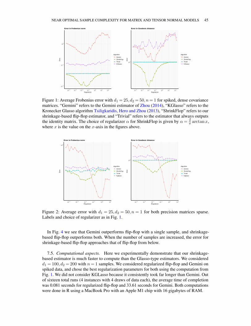
NEAR OPTIMAL SAMPLE COMPLEXITY FOR MATRIX AND TENSOR NORMAL MODELS 45
10−2
10−1
100
10−4 10−3 10−2 10−1 100 101 102
Regularizer
Err
or
Algorithm
Gemini
ShrinkFlop
Trivial
KGlasso
Error in Frobenius norm
100
10−4 10−3 10−2 10−1 100 101 102
Regularizer
Err
or
Algorithm
Gemini
ShrinkFlop
Trivial
KGlasso
Error in Geodesic distance
Figure 1: Average Frobenius error with d1 = 25, d2 = 50, n= 1 for spiked, dense covariancematrices. “Gemini” refers to the Gemini estimator of Zhou (2014), “KGlasso” refers to theKronecker Glasso algorithm Tsiligkaridis, Hero and Zhou (2013), “ShrinkFlop” refers to ourshrinkage-based flip-flop estimator, and “Trivial” refers to the estimator that always outputsthe identity matrix. The choice of regularizer α for ShrinkFlop is given by α= 2
π arctanx,where x is the value on the x-axis in the figures above.
100
10−4 10−3 10−2 10−1 100 101
Regularizer
Err
or
Algorithm
Gemini
ShrinkFlop
Trivial
Kglasso
Error in Frobenius norm
100
10−4 10−3 10−2 10−1 100 101
Regularizer
Err
or
Algorithm
Gemini
ShrinkFlop
Trivial
Kglasso
Error in Geodesic distance
Figure 2: Average error with d1 = 25, d2 = 50, n = 1 for both precision matrices sparse.Labels and choice of regularizer as in Fig. 1.
In Fig. 4 we see that Gemini outperforms flip-flop with a single sample, and shrinkage-based flip-flop outperforms both. When the number of samples are increased, the error forshrinkage-based flip-flop approaches that of flip-flop from below.
7.5. Computational aspects. Here we experimentally demonstrate that our shrinkage-based estimator is much faster to compute than the Glasso-type estimators. We consideredd1 = 100, d2 = 200 with n= 1 samples. We considered regularized flip-flop and Gemini onspiked data, and chose the best regularization parameters for both using the computation fromFig. 1. We did not consider KGLasso because it consistently took far longer than Gemini. Outof sixteen total runs (4 instances with 4 draws of data each), the average time of completionwas 0.081 seconds for regularized flip-flop and 33.61 seconds for Gemini. Both computationswere done in R using a MacBook Pro with an Apple M1 chip with 16 gigabytes of RAM.
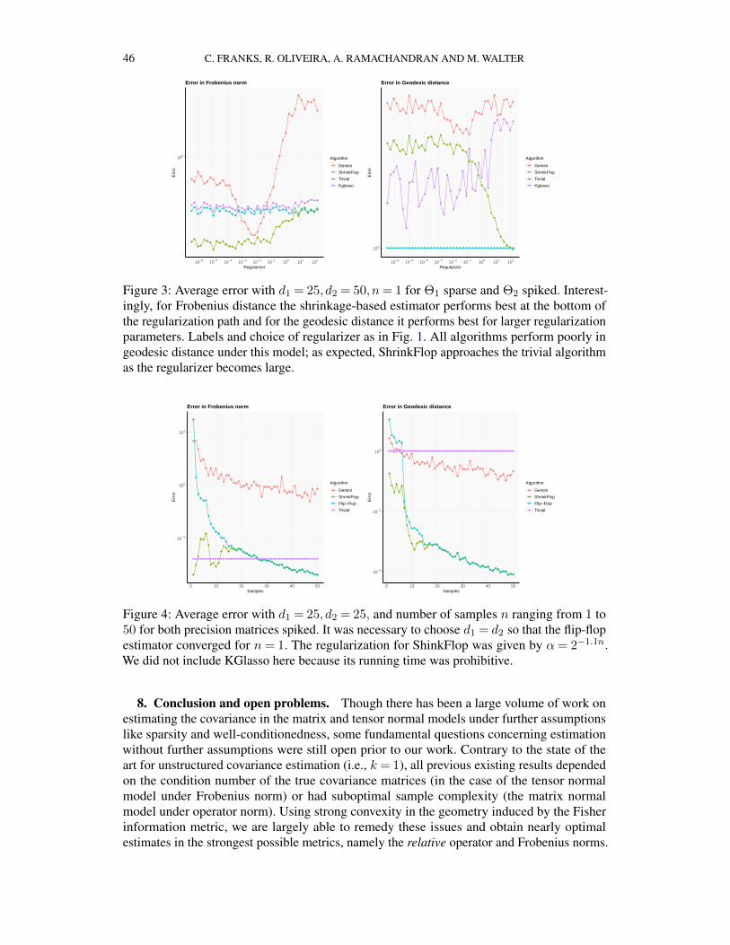
46 C. FRANKS, R. OLIVEIRA, A. RAMACHANDRAN AND M. WALTER
100
10−6 10−5 10−4 10−3 10−2 10−1 100 101 102
Regularizer
Err
or
Algorithm
Gemini
ShrinkFlop
Trivial
Kglasso
Error in Frobenius norm
100
10−6 10−5 10−4 10−3 10−2 10−1 100 101 102
Regularizer
Err
or
Algorithm
Gemini
ShrinkFlop
Trivial
Kglasso
Error in Geodesic distance
Figure 3: Average error with d1 = 25, d2 = 50, n= 1 for Θ1 sparse and Θ2 spiked. Interest-ingly, for Frobenius distance the shrinkage-based estimator performs best at the bottom ofthe regularization path and for the geodesic distance it performs best for larger regularizationparameters. Labels and choice of regularizer as in Fig. 1. All algorithms perform poorly ingeodesic distance under this model; as expected, ShrinkFlop approaches the trivial algorithmas the regularizer becomes large.
10−1
100
101
0 10 20 30 40 50Samples
Err
or
Algorithm
Gemini
ShrinkFlop
Flip−Flop
Trivial
Error in Frobenius norm
10−2
10−1
100
0 10 20 30 40 50Samples
Err
or
Algorithm
Gemini
ShrinkFlop
Flip−Flop
Trivial
Error in Geodesic distance
Figure 4: Average error with d1 = 25, d2 = 25, and number of samples n ranging from 1 to50 for both precision matrices spiked. It was necessary to choose d1 = d2 so that the flip-flopestimator converged for n= 1. The regularization for ShinkFlop was given by α= 2−1.1n.We did not include KGlasso here because its running time was prohibitive.
8. Conclusion and open problems. Though there has been a large volume of work onestimating the covariance in the matrix and tensor normal models under further assumptionslike sparsity and well-conditionedness, some fundamental questions concerning estimationwithout further assumptions were still open prior to our work. Contrary to the state of theart for unstructured covariance estimation (i.e., k = 1), all previous existing results dependedon the condition number of the true covariance matrices (in the case of the tensor normalmodel under Frobenius norm) or had suboptimal sample complexity (the matrix normalmodel under operator norm). Using strong convexity in the geometry induced by the Fisherinformation metric, we are largely able to remedy these issues and obtain nearly optimalestimates in the strongest possible metrics, namely the relative operator and Frobenius norms.
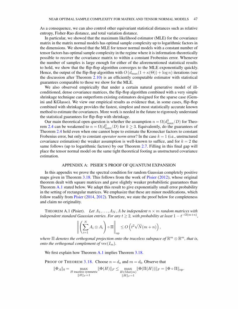
NEAR OPTIMAL SAMPLE COMPLEXITY FOR MATRIX AND TENSOR NORMAL MODELS 47
As a consequence, we can also control other equivariant statistical distances such as relativeentropy, Fisher-Rao distance, and total variation distance.
In particular, we showed that the maximum likelihood estimator (MLE) for the covariancematrix in the matrix normal models has optimal sample complexity up to logarithmic factors inthe dimensions. We showed that the MLE for tensor normal models with a constant number oftensor factors has optimal sample complexity in the regime where it is information-theoreticallypossible to recover the covariance matrix to within a constant Frobenius error. Wheneverthe number of samples is large enough for either of the aforementioned statistical resultsto hold, we show that the flip-flop algorithm converges to the MLE exponentially quickly.Hence, the output of the flip-flop algorithm with O (dmax(1 + κ(Θ)) + logn) iterations (seethe discussion after Theorem 2.10) is an efficiently computable estimator with statisticalguarantees comparable to those we show for the MLE.
We also observed empirically that under a certain natural generative model of ill-conditioned, dense covariance matrices, the flip-flop algorithm combined with a very simpleshrinkage technique can outperform existing estimators designed for the sparse case (Gem-ini and KGlasso). We view our empirical results as evidence that, in some cases, flip-flopcombined with shrinkage provides the fastest, simplest and most statistically accurate knownmethod to estimate the covariances. More work is needed in the future to rigorously understandthe statistical guarantees for flip-flop with shrinkage.
Our main theoretical open question is whether the assumption n= Ω(d3max/D) for Theo-
rem 2.4 can be weakened to n= Ω(d2max/D) for k ≥ 3. Equivalently, do the guarantees of
Theorem 2.4 hold even when one cannot hope to estimate the Kronecker factors to constantFrobenius error, but only to constant operator norm error? In the case k = 1 (i.e., unstructuredcovariance estimation) the weaker assumption is well-known to suffice, and for k = 2 thesame follows (up to logarithmic factors) by our Theorem 2.7. Filling in this final gap willplace the tensor normal model on the same tight theoretical footing as unstructured covarianceestimation.
APPENDIX A: PISIER’S PROOF OF QUANTUM EXPANSION
In this appendix we prove the spectral condition for random Gaussian completely positivemaps given in Theorem 3.18. This follows from the work of Pisier (2012), whose originaltheorem dealt with square matrices and gave slightly weaker probabilistic guarantees thanTheorem A.1 stated below. We adapt this result to give exponentially small error probabilityin the setting of rectangular matrices. We emphasize that these are minor modifications, whichfollow readily from Pisier (2014, 2012). Therefore, we state the proof below for completenessand claim no originality.
THEOREM A.1 (Pisier). Let A1, . . . ,AN ,A be independent n×m random matrices withindependent standard Gaussian entries. For any t≥ 2, with probability at least 1− t−Ω(m+n),∥∥∥∥∥
(N∑i=1
Ai ⊗Ai
)Π
∥∥∥∥∥op
≤O(t2√N(m+ n)
),
where Π denotes the orthogonal projection onto the traceless subspace of Rm ⊗Rm, that is,onto the orthogonal complement of vec(Im).
We first explain how Theorem A.1 implies Theorem 3.18.
PROOF OF THEOREM 3.18. Choose n= da and m= db. Observe that
‖ΦA‖0 = maxH traceless symmetric
‖H‖F=1
‖Φ(H)‖F ≤ maxH∈Mat(m)‖H‖F=1
‖Φ(Π(H))‖F = ‖Φ Π‖op.
48 C. FRANKS, R. OLIVEIRA, A. RAMACHANDRAN AND M. WALTER
Here we identified Mat(m) ∼= Rm ⊗ Rm, so Π identifies with the orthogonal projectiononto the traceless matrices, and we used that ‖Π(H)‖F ≤ ‖H‖F , since Π is an orthogonalprojection. Using Eq. (3.11), the result now follows from Theorem A.1.
In the remainder we discuss the proof of Theorem A.1. The proof proceeds by a symmetriza-tion trick, followed by the trace method. We first state some relevant bounds on Gaussianrandom variables and then give the proof of Theorem A.1.
We will often use the following estimate of the operator norm of a standard Gaussian n×mrandom matrix A (see Theorem 5.32 in Vershynin (2012)),
(A.1) E‖A‖op ≤√n+√m.
THEOREM A.2. Let A be a centered Gaussian random variable that takes values in aseparable Banach space with norm ‖ · ‖. Then ‖A‖ satisfies the following concentration andmoment inequalities with parameter σ2 := supE〈ξ,A〉2 | ‖ξ‖∗ ≤ 1, where ‖ · ‖∗ denotesthe dual norm:
∀t > 0: Pr(∣∣‖A‖ −E‖A‖
∣∣≥ t)≤ 2 exp(−Ω(t2)
σ2
), and
(A.2) ∀p≥ 1: E‖A‖p ≤ (2E‖A‖)p +O(σ√p)p.
PROOF. The first statement on concentration is exactly Theorem 1.5 in Pisier (1986). Forthe second, we consider the random variable X := 1
σ (‖A‖ −E‖A‖). Then the equivalence inLemma 5.5 of Vershynin (2012) gives the moment bound(
E|X|p)1/p
=1
σ
(E∣∣∣‖A‖ −E‖A‖
∣∣∣p)1/p≤O(
√p).
The moment bound in the theorem now follows by rearranging as
E‖A‖p = E(E‖A‖+ σX
)p≤ 2p
((E‖A‖)p +O(σ
√p)p),
where the last step was by the simple inequality (a+ b)p ≤ 2p(|a|p + |b|p).
Below, we calculate the σ2 parameter in Theorem A.2 with regards to our random matrixsetting.
COROLLARY A.3. Let A be an n×m matrix with independent standard Gaussian entries.Then the random variable ‖A‖op satisfies the conclusions of Theorem A.2 with σ2 = 1.
PROOF. Note that the dual norm is the trace norm ‖·‖tr, hence the concentration parametercan be estimated as
σ2 = supE〈ξ,A〉2 | ‖ξ‖tr ≤ 1
= sup
‖ξ‖2F | ‖ξ‖tr ≤ 1
= 1,
where we first used that 〈ξ,A〉 is distributed the same as ‖ξ‖FA11 by orthogonal invariance,and then that the trace norm dominates the Frobenius norm, with equality attained for exampleby ξ =E11.
We will also use the the Schatten p-norms ‖A‖p = (Tr[(ATA)
p
2
])
1
p , which generalize thetrace, Frobenius, and operator norms. They satisfy the following Hölder inequality for p≥ 1:∣∣∣∣∣Tr
p∏i=1
Ai
∣∣∣∣∣≤p∏i=1
‖Ai‖p,(A.3)
NEAR OPTIMAL SAMPLE COMPLEXITY FOR MATRIX AND TENSOR NORMAL MODELS 49
PROOF OF THEOREM A.1. The operator we want to control has entries which are depen-dent in complicated ways. We first begin with a standard symmetrization trick to linearize(compare the proof of Lemma 4.1 in Pisier (2014)). A single entry of Ai ⊗ Ai is either aproduct gg′ of two independent standard Gaussians, or the square g2 of a single standardGaussian. In expectation, we have Egg′ = 0,Eg2 = 1, and so the expected matrix is
E
(N∑i=1
Ai ⊗Ai
)=N vec(In) vec(Im)T .
Accordingly, after projection we have
E
(N∑i=1
Ai ⊗Ai
)Π = 0.
Therefore we may add an independent copy: Let B1, . . . ,BN be independent n×m randommatrices with standard Gaussian entries, that are also independent from A1, . . . ,AN . Then,(
N∑i=1
Ai ⊗Ai
)Π = EB
(N∑i=1
Ai ⊗Ai −N∑i=1
Bi ⊗Bi
)Π
and hence, for any p≥ 1,
E
∥∥∥∥∥(
N∑i=1
Ai ⊗Ai
)Π
∥∥∥∥∥p
op
≤ E
∥∥∥∥∥(
N∑i=1
Ai ⊗Ai −N∑i=1
Bi ⊗Bi
)Π
∥∥∥∥∥p
op
by Jensen’s inequality, as ‖·‖pop is convex as the composition of the norm ‖·‖op with theconvex and nondecreasing function x→ xp. Now note (Ai,Bi) has the same distribution as(Ai+Bi√
2, Ai−Bi√
2), so the right-hand side is equal to
E
∥∥∥∥∥1
2
(N∑i=1
(Ai +Bi)⊗ (Ai +Bi)−N∑i=1
(Ai −Bi)⊗ (Ai −Bi)
)Π
∥∥∥∥∥p
op
= E
∥∥∥∥∥(
N∑i=1
Ai ⊗Bi +
N∑i=1
Bi ⊗Ai
)Π
∥∥∥∥∥p
op
≤ 2pE
∥∥∥∥∥N∑i=1
Ai ⊗Bi
∥∥∥∥∥p
op
Thus, we have proved that
E
∥∥∥∥∥(
N∑i=1
Ai ⊗Ai
)Π
∥∥∥∥∥p
op
≤ 2pE
∥∥∥∥∥N∑i=1
Ai ⊗Bi
∥∥∥∥∥p
op
.(A.4)
Note that we have lost the projection and removed the dependencies. Next we use the tracemethod to bound the right-hand side of Eq. (A.4). That is, we approximate the operatornorm by the Schatten p-norm for a large enough p and control these Schatten norms usingconcentration of moments of Gaussians (compare the proof of Theorem 16.6 in Pisier (2012)).For any q ≥ 1,
E
∥∥∥∥∥N∑i=1
Ai ⊗Bi
∥∥∥∥∥2q
2q
= ETr
∑i,j∈[N ]
ATi Aj ⊗BTi Bj
q =
∑i,j∈[N ]q
ETr(ATi1Aj1 · · ·A
TiqAjq ⊗B
Ti1Bj1 · · ·B
TiqBjq
)
50 C. FRANKS, R. OLIVEIRA, A. RAMACHANDRAN AND M. WALTER
=∑
i,j∈[N ]q
ETr(ATi1Aj1 · · ·A
TiqAjq
)ETr
(BTi1Bj1 · · ·B
TiqBjq
)where we used the independence of Ai and Bi in the last step. Now, the expectation of amonomial of independent standard Gaussian random variables is always nonnegative. Thusthe same is true for ETr(ATi1Aj1 · · ·A
TiqAjq), so we can upper bound the sum term by term as∑
i,j∈[N ]q
ETr(ATi1Aj1 · · ·A
TiqAjq
)ETr
(BTi1Bj1 · · ·B
TiqBjq
)≤
∑i,j∈[N ]q
ETr(ATi1Aj1 · · ·A
TiqAjq
)E(‖Bi1‖2q‖Bj1‖2q · · · ‖Biq‖2q‖Bjq‖2q
)≤
∑i,j∈[N ]q
ETr(ATi1Aj1 · · ·A
TiqAjq
)E(‖B1‖2q2q
)
=
(E‖
N∑i=1
Ai‖2q2q
)(E‖A‖2q2q
)=N q
(E‖A‖2q2q
)2.
In the first step we used Hölder’s inequality (A.3) for the Schatten norm. The second step holdssince E‖Bi‖k2q ≤ (E‖Bi‖2q2q)
k
2q by Jensen’s inequality, so we can collect like terms together.Next, we used that the Bi have the same distribution as A. In the last step, we used that
∑iAi
has the same distribution as√NA. Accordingly, we obtain for q ≥ 1,
E
∥∥∥∥∥N∑i=1
Ai ⊗Bi
∥∥∥∥∥2q
2q
≤N q(E‖A‖2q2q
)2,
and hence
E
∥∥∥∥∥(
N∑i=1
Ai ⊗Ai
)Π
∥∥∥∥∥2q
op
≤ 4q E
∥∥∥∥∥N∑i=1
Ai ⊗Bi
∥∥∥∥∥2q
op
≤ 4q E
∥∥∥∥∥N∑i=1
Ai ⊗Bi
∥∥∥∥∥2q
2q
≤ (4N)q(E‖A‖2q2q
)2≤ (4N)qm2
(E‖A‖2qop
)2.
The first inequality is Eq. (A.4), and in the last inequality we used that A ∈Mat(n,m) hasrank≤m, and therefore ‖A‖2q2q ≤m‖A‖
2qop. To bound the right-hand side, we use Theorem A.2,
applied to the random variableA in the Banach space Mat(n,m) with the operator norm ‖·‖op.Then, σ2 = 1, as computed in Corollary A.3, and we find that
E
∥∥∥∥∥(
N∑i=1
Ai ⊗Ai
)Π
∥∥∥∥∥2q
op
≤ (4N)qm2(
(2E‖A‖op)2q + (C√q)2q
)2.
where C > 0 is a universal constant implied by the big-O notation in Eq. (A.2). We can boundthe first term E‖A‖op ≤
√m+
√n by Eq. (A.1), so for q = 2(m+ n), we can upper bound
the mean by
E
∥∥∥∥∥(
N∑i=1
Ai ⊗Ai
)Π
∥∥∥∥∥2q
op
≤ 4m2(
(max2,C)2 · q ·√
4N)2q
.
NEAR OPTIMAL SAMPLE COMPLEXITY FOR MATRIX AND TENSOR NORMAL MODELS 51
Finally, we can use Markov’s inequality to see that, for C ′ =√
2 max2,C, the event∥∥∥∥∥(
N∑i=1
Ai ⊗Ai
)Π
∥∥∥∥∥op
≤ (C ′t)2 · (m+ n) ·√
4N(A.5)
holds up to failure probability at most
4m2
((max2,C)2 · q ·
√4N
(C ′t)2 · (m+ n) ·√
4N
)2q
≤ 4m2t−2q ≤ t−Ω(m+n),
where the first step was by our choice of q = 2(m+ n) and of C ′ =√
2 max2,C, and thefinal inequality was by the fact that t≥ 2, so the prefactor 4m2 can be absorbed at the cost ofslightly changing the constant in the exponent.
APPENDIX B: PROOF OF THE ROBUSTNESS LEMMA
In this appendix we give a proof of Lemma 3.20, which shows that strong convexity ata particular point implies strong convexity nearby. First note that by Remark 3.15, we have∇2fx(Θ) =∇2fx′ where x′ = Θ1/2x. Thus we need only bound the difference between fxand fx′ for ‖ log Θ‖op small, Θ ∈ P. For a matrix δa in Mat(da), we use e(δa)(a) to denote
e(δa)(a) = Id1 ⊗ · · · ⊗ Ida−1⊗ eδ ⊗ Ida+1
⊗ · · · ⊗ Idk ,
as in Definition 3.8. We will write Θ1/2 as eδ , where δ =∑k
a=1(δa)(a). We now haveΘ1/2 = eδ = ⊗ka=1e
δa , and 12‖ log Θ‖op = ‖δ‖op =
∑ka=1 ‖δa‖op. To bound the difference
between ∇2fx′ and ∇2fx, we will show each component of the Hessian ∇fx′ (as pre-sented in Lemma 3.14) only changes (from ∇fx) by a small amount under the perturbationx→ x′ := eδx. In particular we will give bounds on each block under each component-wise perturbation x→ e(δa)(a)x, and write the overall perturbation as a sequence of suchcomponent-wise perturbations. For convenience, we adopt the short-hand
ρx :=1
nDxxT .
We begin with an easy fact relating the exponential map and matrix norms.
FACT B.1. For all symmetric d× d matrices A such that ‖A‖op ≤ 1, we have
‖eA − I‖op ≤ 2‖A‖op
and
‖eA − I‖F ≤ 2‖A‖F .
The 00 component of the Hessian is a scalar ∇200f = Tr[ρ], and for a≥ 1 we think of each 0a
component as a vector: ∑a
〈z0, (∇20af)Za〉= z0〈ρ,
∑a
√daZ(a)〉
The diagonal components involve only one-body marginals of ρ:
〈Za, (∇2aaf)Za〉= 〈daρ(a),Z2
a〉
And the off-diagonal components involve two-body marginals:
〈Za, (∇2baf)Zb〉= 〈
√dadbρ
(ab),Za ⊗Zb〉.
52 C. FRANKS, R. OLIVEIRA, A. RAMACHANDRAN AND M. WALTER
Therefore in Lemma B.2 and Lemma B.3, we will prove perturbation bounds on one-bodymarginals, and in Lemma B.6 we will prove perturbation bounds on two-body marginals.This will allow us to bound the change in the 0a components, diagonal components, andthe off-diagonal components, respectively. Then, following the structure of the proof ofProposition 3.19, we will collect all the term-wise bounds to prove an overall bound at the endof the section.
LEMMA B.2. For x ∈RD×n and a symmetric matrix δ ∈Mat(da) such that ‖δ‖op ≤ 1,if we denote x′ := eδ(a)x then
‖ρ(a)x′ − ρ
(a)x ‖op ≤ 8‖δ‖op‖ρ(a)
x ‖op.
PROOF. By definition, ‖ρ(a)x′ − ρ
(a)x ‖op = sup‖Z‖1≤1〈Z(a), ρx′ − ρx〉. Let δ′ := eδ − Ia.
Note that ‖δ′‖op ≤ 2‖δ‖op by Fact B.1 and our assumption ‖δ‖op ≤ 1. Now
〈Z(a), ρx′ − ρx〉= 〈Z(a), (I + δ′)aρx(I + δ′)a − ρx〉
= 〈Z, δ′ρ(a)x 〉+ 〈Z,ρ(a)
x δ′〉+ 〈Z, δ′ρ(a)x δ′〉
≤ (2‖δ′‖op + ‖δ′‖2op)‖ρ(a)‖op‖Z‖1
≤ 8‖δ‖op‖ρ(a)‖op.
LEMMA B.3. For x ∈RD×n and symmetric matrix δ ∈Mat(db) such that ‖δ‖op ≤ 1, ifwe denote x′ := eδ(b)x then for b 6= a:
‖ρ(a)x′ − ρ
(a)x ‖op ≤ 2‖δ‖op‖ρax‖op.
PROOF. By definition, ‖ρ(a)x′ − ρ
(a)x ‖op = sup‖Z‖1≤1,Z0 |〈Z(a), ρx′ − ρx〉|.
Let δ′ := eδ − Ib. Note that ‖δ′‖op ≤ 2‖δ‖op by Fact B.1 and our assumption ‖δ‖op ≤ 1.Now
|〈Z(a), ρx′ − ρx〉|= |〈Z(a), eδ(b)ρxe
δ(b) − ρx〉|
= |〈Z(a)δ′(b), ρx〉|= |〈Z ⊗ δ
′, ρ(ab)x 〉|
≤ 〈‖δ′‖opZ ⊗ Ib, ρ(ab)x 〉
= ‖δ′‖op〈Z,ρ(a)x 〉 ≤ 2‖δ‖op‖Z‖1‖ρ(a)
x ‖op.
This is already enough to prove a bound on 0a and aa terms:
COROLLARY B.4. Let x ∈ RD×n be such that ‖daρ(a)x ‖op ≤ 1 + 1
20 , and for b ∈ [k]
let δb ∈Mat(db) be a symmetric matrix such that∑
b ‖δb‖op ≤ 18 . Denoting δ(b) := (δb)(b),
δ =∑
b δ(b) and x′ = eδx, for a≥ 1 we have
‖∇2aaf(e2δ)−∇2
aaf(I)‖op ≤ 25‖δ‖op.

NEAR OPTIMAL SAMPLE COMPLEXITY FOR MATRIX AND TENSOR NORMAL MODELS 53
PROOF. Recall from Lemma 3.14 that 〈Y, (∇2aafx)Y 〉= 〈daρ(a)
x , Y 2〉; thus it is enough toshow that ‖ρ(a)
x′ − ρ(a)x ‖op ≤ 25‖δ‖op/da. We treat the perturbation eδ as the composition of
k perturbations:
x(0) := x→ x(1) := eδ(1)x(0)→ ...→ x(k) := eδ(k)x(k−1) = x′.
We can use Lemma B.2 to handle eδ(a) and Lemma B.3 for the rest. Let Z be a symmetricmatrix.
|〈ρ(a)x′ − ρ
(a)x ,Z〉| ≤
k∑j=1
|〈ρ(a)x(j)− ρ(a)
x(j−1),Z〉|
≤k∑j=1
8‖δj‖op‖ρ(a)x(j−1)
‖op‖Z‖1.
Where the last inequality is due to Lemmas B.2 and B.3. To bound each term in the right-handside, note that by Lemmas B.2 and B.3 we have
‖ρ(a)x(j)‖op ≤ ‖ρ(a)
x(j)− ρ(a)
x(j−1)‖op + ‖ρ(a)
x(j−1)‖op ≤ (1 + 8‖δj‖op)‖ρ(a)
x(j−1)‖op
and hence by induction the jth term in the sum is at most
8‖δj‖op
(k∏l=1
(1 + 8‖δl‖op)
)‖ρ(a)
x ‖op‖Z‖1.
By our assumption that∑
l ‖δl‖op ≤ 1/8, this is at most 8‖δj‖ope8∑‖δl‖op‖ρ(a)
x ‖op‖Z‖1 ≤8e‖δj‖op‖ρ(a)
x ‖op‖Z‖1. Adding up the terms and using that ‖δ‖op =∑‖δ(c)‖op, the overall
sum is then at most 8e‖δ‖op‖ρ(a)x ‖op‖Z‖1. Using our assumption on ‖daρ(a)
x ‖op completesthe proof.
COROLLARY B.5. Let x ∈RD×n be such that ‖daρ(a)x ‖op ≤ 1 + 1
20 , and for b ∈ [k] let δbbe symmetric matrices such that ‖
∑b δ(b)‖op =
∑b ‖δb‖op ≤ 1
8 , where once again we denoteδ(b) := (δb)(b) and δ :=
∑b δ(b). Denoting x′ := eδx, for a≥ 1 we have
|∇200fx′ −∇2
00fx| ≤ 5‖δ‖op
and ‖∇20afx′ −∇2
0afx‖op ≤ 25‖δ‖op.
PROOF. Recall from Lemma 3.14 that the 00 component of the Hessian is just the scalarTrρ. The assumption that ‖daρ(a)
x ‖op ≤ 1 + 120 implies Tr[ρx] = Trρ
(a)x ≤ 1 + 1/20. Now we
can use the approximation for eδ in Fact B.1:
|Tr[ρx′ − ρx]|= |〈ρx, e2δ − I〉| ≤Tr[ρx]‖e2δ − I‖op ≤ 5‖δ‖op
In the last step we used our bound on Tr[ρx]. The 0a component is a vector, so it is enough tobound the inner product with any traceless matrix Z of unit Frobenius norm:
|〈ρ(a)x′ − ρ
(a)x ,√daZ〉| ≤ ‖ρ(a)
x′ − ρ(a)x ‖op
√da‖Z‖1.
In the proof of Corollary B.4 we showed under the same assumptions we have ‖ρ(a)x′ −
ρ(a)x ‖op ≤ 25‖δ‖op/da, from which it follows that the above is at most 25‖δ‖op‖Z‖F .
The off-diagonal components require the following two lemmata on bipartite marginals:
54 C. FRANKS, R. OLIVEIRA, A. RAMACHANDRAN AND M. WALTER
LEMMA B.6. For x ∈RD×n and a symmetric matrix δ ∈Mat(dc) such that ‖δ‖op ≤ 18 ;
if we denote x′ := eδ(c)x, then for c ∈ a, b we have
supY ∈S0
da,Z∈S0
db
|〈ρ(ab)x′ − ρ
(ab)x , Y ⊗Z〉|
‖Y ‖F ‖Z‖F≤ 3‖δ‖op sup
Y ∈Sda ,Z∈Sdb
〈ρ(ab)x , Y ⊗Z〉‖Y ‖F ‖Z‖F
.
Note that S0d are traceless symmetric matrices, whereas Sd are symmetric matrices.
PROOF. By taking adjoints, we can assume w.l.o.g. that c= b. Let R : Mat(db)→Mat(db)be defined as R(Z) := eδZeδ . Then
|〈ρ(ab)x′ − ρ
(ab)x , Y ⊗Z〉|= |〈ρ(ab)
x , Y ⊗ (R(Z)−Z)〉|The subspace S0
dbis not invariant under R, but we show R≈ I . Let δ′ := eδ − I ; by Fact B.1,
‖δ′‖op ≤ 14 . Now
‖R(Z)−Z‖F ≤ 2‖δ′Z‖F + ‖δ′Zδ′‖F ≤ (2‖δ′‖op + ‖δ′‖2op)‖Z‖F ≤ 3‖δ‖op‖Z‖F .We combine these inequalities and apply a change of variables R(Z)−Z← Z ′ to finish theproof.
supY ∈S0
da,Z∈S0
db
|〈ρ(ab)x′ − ρ
(ab)x , Y ⊗Z〉|
‖Y ‖F ‖Z‖F= supY ∈S0
da,Z∈S0
db
|〈ρ(ab)x , Y ⊗ (R(Z)−Z)〉|‖Y ‖F ‖Z‖F
≤ supY ∈S0
da,Z′∈Sdb
|〈ρ(ab)x , Y ⊗Z ′〉| · 3‖δ‖op
‖Y ‖F ‖Z ′‖F.
LEMMA B.7. For x ∈RD×n and a symmetric matrix δ ∈Mat(dc) such that ‖δ‖op ≤ 18 ;
if we denote x′ := eδ(c)x, then for c 6∈ a, b we have
supY ∈S0
da,Z∈S0
db
|〈ρ(ab)x′ − ρ
(ab)x , Y ⊗Z〉|
‖Y ‖F ‖Z‖F≤ 4‖δ‖op sup
Y ∈Sda ,Z∈Sdb
〈ρ(ab)x , Y ⊗Z〉‖Y ‖F ‖Z‖F
.
PROOF. Let δ′ := e2δ− Ic so that |〈ρ(ab)x′ −ρ
(ab)x , Y ⊗Z〉|= |〈ρ(abc)
x , Y ⊗Z⊗ δ′〉|. We firstassume Y,Z 0, and without loss of generality we assume that ‖Y ‖F = ‖Z‖F = 1. Becauseρ
(abc)x , Y,Z 0, and δ′ ‖δ′‖op · Ic, we have
|〈ρ(abc)x , Y ⊗Z ⊗ δ′〉| ≤ 〈ρ(abc)
x , Y ⊗Z ⊗ ‖δ′‖op · Ic〉
≤ ‖δ′‖op〈ρ(ab)x , Y ⊗Z〉 ≤ 2‖δ‖op〈ρ(ab)
x , Y ⊗Z〉,where the last inequality is by Fact B.1. To finish the proof we decompose Y = Y+−Y−,Z =Z+ −Z−, where Y+, Y−,Z+,Z− are all positive semidefinite, and bound
|〈ρ(ab)x′ − ρ
(ab)x , Y ⊗Z〉| ≤
∑s,t∈+,−
|〈ρ(ab)x′ − ρ
(ab)x , Y ⊗Z〉|
≤∑
s,t∈+,−
2‖δ‖op〈ρ(ab)x , Ys ⊗Zt〉
≤ 2
(sup
Y ∈Sda ,Z∈Sdb
〈ρ(ab)x , Y ⊗Z〉‖Y ‖F ‖Z‖F
)‖δ‖op
∑s,t∈+,−
‖Ys‖F ‖Zt‖F
NEAR OPTIMAL SAMPLE COMPLEXITY FOR MATRIX AND TENSOR NORMAL MODELS 55
The Cauchy Schwarz inequality allows us to bound the summation:∑s,t∈+,−
‖Ys‖F ‖Zt‖F ≤ (2‖Y+‖2F + 2‖Y−‖2F )1/2(2‖Z+‖2F + 2‖Z−‖2F )1/2 = 2‖Y ‖F ‖Z‖F .
Plugging this bound in to the supremum on the left-hand side in the statement of the lemmacompletes the proof.
The following definition will be helpful for translating the above lemmas into statementsabout the Hessian.
DEFINITION B.8. For a linear map M : Mat(d)→Mat(d′), we let ‖M‖0 denote theF → F norm of its restriction to the traceless subspaces S0
d → S0d′ , i.e.
‖M‖0 = supZ∈S0
d
‖M(Z)− TrM(Z)d′ Id′‖F
‖Z‖F.
The following lemma will be helpful.
LEMMA B.9 (Kwok, Lau and Ramachandran (2019)). For x ∈RD×n,
‖∇2abfx‖2F→F ≤ ‖daρ(a)
x ‖op‖dbρ(b)x ‖op.
Analogously to the proof of Corollary B.4, we can now combine Lemma B.6 andLemma B.7 to bound the effect of a perturbation with more than one nontrivial tensor factor.
COROLLARY B.10. Let x ∈ RD×n be such that ‖daρ(a)x ‖op,‖dbρ
(b)x ‖op ≤ 1 + 1
20 , andfor c ∈ [k] let δc be a symmetric matrix such that ‖
∑c δ(c)‖op =
∑c ‖δc‖op ≤ 1
8 . Denotingx′ := eδx, we have
‖∇2abfx′ −∇2
abfx‖0 ≤ 21‖δ‖op
PROOF. First, using Lemma 3.14, we write the left-hand and right-hand sides of theinequalities in Lemma B.6 and Lemma B.7 in terms of the Hessian:
supY ∈S0
da,Z∈S0
db
〈ρ(ab)x′ − ρ
(ab)x , Y ⊗Z〉
‖Y ‖F ‖Z‖F=‖∇2
abfx′ −∇2abfx‖0√
dadb,
and supY ∈Sda ,Z∈Sdb
〈ρ(ab)x , Y ⊗Z〉‖Y ‖F ‖Z‖F
=‖∇2
abfx‖F→F√dadb
.
Using the same iterative strategy as in the proof of Corollary B.4 for the left-hand sides of theabove identities, we have
|〈Y, (∇2abfx′ −∇2
abfx)Z〉| ≤ 20‖δ‖op‖∇2abfx‖F→F ‖Y ‖F ‖Z‖F ,
using Lemma B.6 for a and b and Lemma B.7 for the rest. Finally, we may rewrite Lemma B.9using Lemma 3.14 to find ‖∇2
abfx‖2F→F ≤ ‖daρ(a)x ‖op‖daρ(a)
x ‖op. Using our assumption that‖daρa‖op,‖dbρb‖op ≤ 1 + 1
20 completes the proof.
Now we can combine the above term-by-term bounds to bound the change in the Hessian.
56 C. FRANKS, R. OLIVEIRA, A. RAMACHANDRAN AND M. WALTER
PROOF OF LEMMA 3.20. The above corollaries (B.5,B.4,B.10) require ‖daρ(a)‖op ≤ 1 +120 , which are implied by our assumption on the gradient:
‖daρ(a)‖op ≤ 1 + |Trρ− 1|+ ‖daρ(a) − (Trρ)Ida‖op
= 1 + |∇0f |+ ‖√da∇af‖op ≤ 1 + 2ε0,
so choosing ε0 ≤ 140 suffices. Recall the expression of the Hessian as a quadratic form
evaluated on Z = (z0,Z1, . . . ,Zk) :
〈Z, (∇2f)Z〉=
z0(∇200f)z0 + 2
∑a
〈z0, (∇20af)Za〉+
∑a
〈Za, (∇2aaf)Za〉+
∑a6=b〈Za, (∇2
abf)Zb〉.
Let x′ := eδx. Then by Corollary B.5 we have a bound on the 0a terms:
|z20(∇2
00fx′ −∇200fx) + 2
∑a
〈z0, (∇20afx′ −∇2
0afx)Za〉|
≤ 5‖δ‖opz20 + (2|z0|)25‖δ‖op
∑a
‖Za‖F ≤ ‖δ‖op(17kz20 + 25
∑a
‖Za‖2F )
In the last step we used Young’s inequality (2pq ≤ p2 + q2) for each term with p = z0,q = ‖Za‖F .
By Corollary B.4 we have a bound on the diagonal terms, and by Corollary B.10 we have abound on the off-diagonal terms:
|∑ab
〈Za, (∇2abfx′ −∇2
abfx)Zb〉| ≤ ‖δ‖op
25∑a
‖Za‖2F + 21∑a6=b‖Za‖F ‖Zb‖F
≤ (25 + 21(k− 1))‖δ‖op
(∑a
‖Za‖2F
)So combining all three terms we see:
|〈Z, (∇2fx′ −∇2fx)Z〉| ≤ ‖δ‖op
(17kz2
0 + (25 + 25 + 21(k− 1))∑a
‖Za‖2F
)
≤ 50k‖δ‖op
(z2
0 +∑a
‖Za‖2F
)= 50k‖δ‖op‖Z‖2.
Note that this also gives an upper bound for ‖∇2fx′‖op.
APPENDIX C: THE CHEEGER CONSTANT OF A RANDOM OPERATOR
In this appendix we prove Theorem 4.5, which asserts that a random completely positivemap with sufficiently many Kraus operators is an almost quantum expander with exponentiallysmall failure probability. To prove the theorem, we first define the Cheeger constant ofcompletely positive map. This is similar to a concept defined in Hastings (2007).
NEAR OPTIMAL SAMPLE COMPLEXITY FOR MATRIX AND TENSOR NORMAL MODELS 57
DEFINITION C.1. Let Φ: Mat(d2) → Mat(d1) be a completely positive map. TheCheeger constant ch(Φ) is given by
ch(Φ) := minΠ1,Π2
0<vol(Π1,Π2)≤ 1
2vol(Id1 ,Id2 )
φ(Π1,Π2)
where Π1 : Cd1 → Cd1 and Π2 : Cd2 → Cd2 are orthogonal projections, and the conduc-tance φ(Π1,Π2) of the “cut” Π1,Π2 is defined to be
φ(Π1,Π2) :=cut(Π1,Π2)
vol(Π1,Π2),
where
vol(Π1,Π2) := Tr Φ(Π2) + TrΦ∗(Π1),
cut(Π1,Π2) := Tr(Id1 −Π1)Φ(Π2) + TrΠ1Φ(Id2 −Π2)
= Tr(Id1 −Π1)Φ(Π2) + TrΦ∗(Π1)(Id2 −Π2).
The key connection that we will leverage to prove Theorem 4.5 is that a large Cheegerconstant implies quantum expansion:
LEMMA C.2 (Franks and Moitra (2020), Remark 5.5). There exist absolute con-stants c,C > 0 such that if Φ is a completely positive map that is ε-doubly balanced forsome ε < c ch(Φ)2, then Φ is an (ε, η)-quantum expander, where
η = max
1
2,1− ch(Φ)2 +C
ε
ch(Φ)2
.
For intuition, consider a weighed bipartite graphG on [d1]∪ [d2]. The projections Π1 and Π2
are analogous to subsets A ⊂ [d1] and B ⊂ [d2], respectively. The quantity vol(Π1,Π2) isanalogous to the total mass of the edges adjacent to A plus that of the edges adjacent to B,which is the volume of A∪B considered as a cut of G. The quantity cut(Π1,Π2) correspondsto the total mass of the edges between A∪B and its complement, that is, to the weight of thecut defined by A∪B. In fact, if the Cheeger constant were defined with Π1 and Π2 restrictedto be coordinate projections, it would be exactly the Cheeger constant of the bipartite graph on[d1] and [d2] with edge (i, j) weighted by Treie
Ti Φ(eje
Tj ), and the volume and the cut would
be the same as the volume and the cut on that bipartite graph.For the remainder of this section let Φ = ΦX whereX1, . . . ,Xn are random d1×d2 matrices
with independent standard Gaussian entries. In this case, each edge-weight TreieTi Φ(eje
Tj )
of the bipartite graph is an independent χ2 random variable with n degrees of freedom.Accordingly:
LEMMA C.3. Let Π1 : Cd1→Cd1 , Π2 : Cd2→Cd2 be orthogonal projections of rank r1
and r2, respectively. Then cut(Π1,Π2), vol(Π1,Π2), vol(Id1 , Id2) are jointly distributed as
R1, R1 + 2R2, 2R1 + 2R2 + 2R3,
where R1, R2, R3 are independent χ2 random variables with F1 := nr1(d2− r2) +nr2(d1−r1), F2 := nr1r2, and F3 := n(d1 − r1)(d2 − r2) degrees of freedom, respectively.
PROOF. As the distribution of ΦX is invariant under the action (U1,U2) · ΦX(Y ) =U1ΦX(UT2 Y U2)UT1 of unitary matrices U1,U2, the joint distribution of cut(Π1,Π2),vol(Π1,Π2) depends only on the rank of Π1, Π2. Thus we may compute in the case that Π1
and Π2 are coordinate projections, in which case one may verify the fact straightforwardly;see the discussion above.
58 C. FRANKS, R. OLIVEIRA, A. RAMACHANDRAN AND M. WALTER
We next show a sufficient condition for the Cheeger constant being bounded away from 1that is amenable to the previous lemma.
LEMMA C.4. Let Φ be a completely positive map and δ < 0.005 such that the followinghold for all orthogonal projections Π1 : Cd1→Cd1 , Π2 : Cd2→Cd2 , not both zero, where wedenote by r1, r2 the ranks of Π1 and Π2, respectively, and abbreviate F1 := nr1(d2 − r2) +nr2(d1 − r1), and F2 := nr1r2 as in Lemma C.3:
1. If F2 ≥ 49nd1d2, then
vol(Π1,Π2)≥(
101
200− δ)
vol(Id1 , Id2) = (1.01− 2δ) TrΦ(Id2).(C.1)
2. If F2 <49nd1d2 and vol(Π1,Π2)> 0, then
vol(Π1,Π2)≤(
4
3+ δ
)(F1 + 2F2) and cut(Π1,Π2)≥
(2
3− δ)F1.(C.2)
Then ch(Φ)≥ 16 −O(δ).
PROOF. The first assumption implies we only need to reason about the case that F2 <49nd1d2. This is because the minimization in the definition of the Cheeger constant is over Π1,Π2 such that vol(Π1,Π2)≤Tr Φ(Id2). Therefore, the second assumption implies that
ch(Φ)≥43 + δ23 − δ
minF2<
4
9nd1d2
F1
F1 + 2F2=
(1
2−O(δ)
)min
r1r2<4
9d1d2
F1
F1 + 2F2.
It suffices to show that F1/(F1 + 2F2)≥ 1/3 provided r1r2 <49d1d2. Indeed, if either r1 = 0
or r2 = 0, then F2 = 0 and F1 > 0 and the claim holds. Otherwise, if r1 > 0 and r2 > 0, thenF1
F1 + 2F2=r1d2 + r2d1 − 2r1r2
r1d2 + r2d1= 1− 2r1r2
r1d2 + r2d1
= 1−√r1r2
d1d2
2√r1d2r2d1
+√
r2d1r1d2
≥ 1−√
4
9=
1
3.
In the last inequality we used that a+ a−1 ≥ 2 for all a > 0 and that r1r2 <49d1d2.
Next we use Lemma C.3 to show that for a random completely positive map, the events inLemma C.4 hold with high probability for any fixed Π1 and Π2. We also need a third boundwhich we will use to transfer properties of a δ-net to the whole space of projections.
LEMMA C.5. Suppose d1 ≤ d2. Let Π1 : Cd1 → Cd1 , Π2 : Cd2 → Cd2 be orthogonalprojections of rank r1 and r2, respectively such that r1 + r2 > 0. Let F1 := nr1(d2 − r2) +nr2(d1 − r1) and F2 = nr1r2. Then, the following holds for the random completely positivemap Φ = ΦX :
1. If F2 ≥ 49nd1d2, then Eq. (C.1) holds with δ = 0 with probability at least 1− e−Ω(nd1d2).
2. If F2 <49nd1d2, then Eq. (C.2) holds with δ = 0 with probability at least 1− e−Ω(F1).
3. Finally, vol(Π1,Π2)≥ 14d2
vol(Id1 , Id2) with probability at least 1− e−Ω(F1+2F2).
PROOF. Recall from Lemma C.3 that cut(Π1,Π2), vol(Π1,Π2), vol(Id1 , Id2) are jointlydistributed as R1, R1 + 2R2, 2R1 + 2R2 + 2R3 for R1,R2,R3 independent χ2 randomvariables with F1, F2, and F3 = n(d1− r1)(d2− r2) degrees of freedom, respectively. In viewof Eqs. (C.1) and (C.2) with δ = 0, it is thus enough to show that
NEAR OPTIMAL SAMPLE COMPLEXITY FOR MATRIX AND TENSOR NORMAL MODELS 59
1. If F2 ≥ 49nd1d2, then R2 ≥ 1
99R1 + 10199 R3 with probability 1− e−Ω(nd1d2).
2. If F2 <49nd1d2, then R1 + 2R2 ≤ 4
3(F1 + 2F2) and R1 ≥ 23F1 hold with probability
1− e−Ω(F1).3. R1 + 2R2 ≥ 2
3(F1 + 2F2) and R1 +R2 +R3 ≤ 43(F1 + F2 + F3) with probability 1−
e−Ω(F1+2F2).
Indeed, the first (resp. second) item above implies the first (resp. second) item in the lemma bysubstituting the expressions for vol and cut of (π1, π2) and (Id1 , Id2) in terms of R1,R2,R3.The last item follows from the same reasoning combined with the inequality F1 + 2F2 ≥1d2
(F1 + F2 + F3) for r1, r2 not both zero and the fact that d1 ≤ d2.All three follow from standard results for concentration of χ2 random variables; see
e.g. Wainwright (2019). We only prove the first item; the second and third items are straight-forward. To prove the first item, we first reason about the case when one of r1 = 0.
note that F1 + 2F2 ≥ 43(F1 + F2 + F3), because
F1 + 2F2
F1 + F2 + F3=r1
d1+r2
d2=
√r1r2
d1d2
(√r1d2
d1r2+
√d1r2
r1d2
)≥√
4
9· 2 =
4
3.
In particular, F2 ≥ 23(F2 + F3) and F2 ≥ 1
6(F1 + F2).We first reason about the ratio between R2 and R3 using the first inequality. With prob-
ability 1 − e−cF2 ≥ 1 − e−Ω(nd1d2), it holds that R2 ≥ 89F2 and R2 + R3 ≤ 10
9 (F2 + F3).The latter holds because R2 + R3 is a χ2 random variable with F2 + F3 ≥ F2 degreesof freedom. so R2 ≥ 8
923
910(R2 + R3) = 8
15(R2 + R3), or R2 ≥ 87R3. We next apply the
same reasoning with the inequality F2 ≥ (F1 + F2)/6 to estimate the ratio between R1
and R2. With probability 1 − e−cnd1d2 , we have R2 ≥ 89F2 and R1 + R2 ≤ 10
9 (F1 + F2).Thus R1 ≥ 8
916
910(R1 + R2) = 4
30(R1 + R2), or R2 ≥ 213R1. Together, we obtain that
R2 ≥ 199R1 + 101
9 9R3 with probability 1− e−Ω(nd1d2).
Finally, we show using a net argument that the Cheeger constant is large for all projections.
LEMMA C.6 (Franks and Moitra (2020), Lemma 5.18). For any ε > 0, there is an operatornorm ε-net of the rank-r orthogonal projections Π: Cd→Cd with cardinality eO(dr|log ε|).
As a corollary, the set of pairs of projections Π1, Π2 of rank r1 and r2, respectively, has an(elementwise) operator norm ε-net of cardinality eO((r1d1+r2d2)|log ε|).
LEMMA C.7 (Continuity of cut and volume). Let Π1,Π′1 : Cd1→Cd1 and Π2,Π
′2 : Cd2→
Cd2 be orthogonal projections such that ‖Π1 −Π′1‖op ≤ ε and ‖Π2 −Π′2‖op ≤ ε. Then:
|cut(Π′1,Π′2)− cut(Π1,Π2)| ≤ 2εvol(Id1 , Id2)
and |vol(Π′1,Π′2)− vol(Π1,Π2)| ≤ 2εvol(Id1 , Id2).
PROOF. We begin with the first inequality:
|cut(Π′1,Π′2)− cut(Π1,Π2)| ≤ |Tr Π′1Φ(Id2 −Π′2)−Tr Π1Φ(Id2 −Π2)|
+ |Tr(Id1 −Π′1)Φ(Π′2)−Tr(Id1 −Π1)Φ(Π2)|.
Consider the first term:
|Tr Π′1Φ(Id2 −Π′2)−Tr Π1Φ(Id2 −Π2)|
= |Tr(Π′1 −Π1)Φ(Id2 −Π′2) + TrΠ1Φ(Π2 −Π′2)|
60 C. FRANKS, R. OLIVEIRA, A. RAMACHANDRAN AND M. WALTER
= |Tr(Π′1 −Π1)Φ(Id2 −Π′2) + TrΦ∗(Π1)(Π2 −Π′2)|
≤ ‖Π′1 −Π1‖op‖Φ(Id2 −Π′2)‖tr + ‖Π2 −Π′2‖op‖Φ∗(Π1)‖tr≤ εTr Φ(Id2) + εTr Φ∗(Id1) = εvol(Id1 , Id2).
The same inequality for the second term follows by symmetry. The proof of the secondinequality is similar.
PROPOSITION C.8 (Cheeger constant lower bound). There is a universal constant C > 0such that the following holds: If d1 ≤ d2, d2 > 1, and n≥ C d2
d1log(d2), then ch(Φ) = Ω(1)
with probability 1− e−Ω(nd1).
PROOF. Let ε= cd2
for some sufficiently small constant c > 0. For r1 ≤ d1 and r2 ≤ d2
not both zero, let N (r1, r2) denote an (elementwise) operator norm ε-net for the set of pairsof projections of rank r1 and r2, respectively. As discussed below Lemma C.6, we mayassume that |N (r1, r2)| ≤ eO((d1r1+d2r2)|log ε|). Let N =
⋃r1,r2N (r1, r2). We claim that to
establish the lemma it suffices to show that with probability 1− e−Ω(nd1), the following issimultaneously true for all r1, r2 and for all (Π1,Π2) ∈N (r1, r2):
1. If F2 := nr1r2 ≥ 49nd1d2, then Eq. (C.1) holds with δ = 0.
2. If F2 <49nd1d2, then Eq. (C.2) holds with δ = 0.
3. vol(Π1,Π2)≥ 14d2
vol(Id1 , Id2).
To see that this suffices, we only need to show that it implies the hypotheses of Lemma C.4for δ = 32c. Let (Π′1,Π
′2) be an arbitrary pair of projections, not both zero. Let r1 and r2
denote their ranks. Then there exists a pair (Π1,Π2) ∈N (r1, r2) such that ‖Π′1 −Π1‖op ≤ εand ‖Π′2 −Π2‖op ≤ ε. If F2 ≥ 4
9nd1d2,
vol(Π′1,Π′2)≥ vol(Π1,Π2)− 2εvol(Id1 , Id2)
≥(
101
200− 2ε
)vol(Id1 , Id2)≥
(101
200− 2c
)vol(Id1 , Id2),
where the first inequality is Lemma C.7, the second uses the first item above, and finallywe estimate ε≤ c. Thus we have verified that Eq. (C.1) holds for (Π′1,Π
′2), that is, the first
hypothesis of Lemma C.4. If F2 <49nd1d2, then
vol(Π′1,Π′2)≤ vol(Π1,Π2) + 2εvol(Id1 , Id2)≤ (1 + 8εd2) vol(Π1,Π2)
≤ (1 + 8εd2)4
3(F1 + 2F2) =
(4
3+
32
3c
)(F1 + 2F2) ,
where F1 := nr1(d2 − r2) + nr2(d1 − r1), the first inequality is Lemma C.7, the secondinequality uses the third item above, and the third inequality uses the second item above. Onthe other hand,
cut(Π′1,Π′2)≥ cut(Π′1,Π
′2)− 2εvol(Id1 , Id2)≥ cut(Π′1,Π
′2)− 8εd2 vol(Π1,Π2)
≥ 2
3F1 − 8εd2
4
3(F1 + 2F2) =
2
3F1 − 8c
4
3(F1 + 2F2)
≥ 2
3F1 − 32cF1 =
(2
3− 32c
)F1,
again using Lemma C.7, the second and third item above. In the last step we used the fact thatF1 ≥ 1
3(F1 + 2F2) provided F2 <49nd1d2, which we established in the proof of Lemma C.4.
NEAR OPTIMAL SAMPLE COMPLEXITY FOR MATRIX AND TENSOR NORMAL MODELS 61
Thus we have verified that Eq. (C.2) holds for (Π′1,Π′2), which is the remaining hypotheses of
Lemma C.4.To prove the lemma we still need to show that the three conditions above hold with the
desired probability. We show that for fixed r1 and r2, each condition holds with probability atleast 1− eΩ(n(r1d2+d1r2)). By the union bound, this implies that the conditions hold simulta-neously for all r1 ≤ d1 and r2 ≤ d2, not both zero, with the desired probability, because thesum of e−Ω(n(r1d2+d1r2)) over all such r1 and r2 is e−Ω(nd1), using that d1 ≤ d2. Thus fix r1
and r2 as above. We first bound the probability for the first item. By Lemma C.5 and the unionbound, if F2 ≥ 4
9nd1d2 then Eq. (C.1) holds for every (Π1,Π2) ∈N (r1, r2) with probability
1− |N (r1, r2)|e−Ω(nd1d2) ≤ 1− e(d1r1+d2r2)|log ε|e−Ω(n(r1d2+d1r2)) ≤ 1− e−Ω(n(r1d2+d1r2)).
The last step follows by our assumption on n (for a large enough universal constant C > 0),since
(d1r1 + d2r2)|log ε| ≤ d2
d1(r1d2 + d1r2) (log(d2) + |log c|) =O
(d2
d1log(d2)
)· (r1d2 + d1r2).
Next we bound the probability for the second item. By Lemma C.5 and the union bound, ifF2 <
49nd1d2, Eq. (C.2) holds for every (Π1,Π2) ∈N (r1, r2) with probability
1− |N (r1, r2)|e−Ω(F1) ≤ 1− |N (r1, r2)|e−Ω(n(r1d2+r2d1)) ≤ 1− e−Ω(n(r1d2+d1r2)),
where the first step holds since F1 ≥ 13(F1 +2F2) = 1
3n(r1d2 +r2d1) whenever F2 <49nd1d2,
as already used earlier in the proof, and the second step follows as above by our assumptionon n (for large enough C > 0). The probability for the third item can be bounded completelyanalogously.
PROOF OF THEOREM 4.5. Let Φ := ΦX . Since n ≥ C d2d1
logd2, Proposition C.8 showsthat ch(Φ) = Ω(1) with failure probability e−Ω(nd1). The latter is e−Ω(d2t2) using our assump-tion that n≥C d2
d1t2.
Now let ε := t√
d2nd1
, which by the same assumption satisfies ε≤ 1√C
. Moreover, n≥ d2max
Dε2 ,since this is equivalent to our assumption that t≥ 1. Therefore, if we choose C sufficientlylarge then, similarly to the proof of Proposition 3.19, we find using Propositions 3.11 and 3.13that Φ is ε-doubly balanced with failure probability e−Ω(nD) +O(e−Ω(nd1ε2))≤ e−Ω(d2t2).
By making C larger, we can ensure that ε is less than any absolute constant. ThenLemma C.2 applies (with balancedness ε) and shows that Φ is an (ε, η)-quantum expander forsome absolute constant η < 1.
APPENDIX D: PROOF OF CONCENTRATION FOR MATRIX NORMAL MODEL
In this section we prove Lemma 4.7, which shows concentration after one step of theflip-flop algorithm. For convenience, we consider the differently normalized random variableZ = Y/
√nd1. Note that these satisfy Zi = XiΦ
∗X(Id1)
−1/2 = Xi(∑n
i=1XTi Xi)
−1/2. Thuswe wish to prove that ∥∥∥∥∥
n∑i=1
ZiZTi −
d2
d1Id1
∥∥∥∥∥op
≤ t√
d2
nd1.(D.1)
Since we are interested in the spectral norm, we will consider the random variable〈ξ,∑n
i=1ZiZTi ξ〉 for a fixed unit vector ξ ∈ Rd1 . We will show that this variable is highly
concentrated, and apply a union bound over a net of the unit vectors. To show the concentration,we first cast 〈ξ,
∑ni=1ZiZ
Ti ξ〉 as the inner product between a random orthogonal projection
62 C. FRANKS, R. OLIVEIRA, A. RAMACHANDRAN AND M. WALTER
and a fixed one. Since each Zi is a d1×d2 matrix, we can consider Z as an nd1×d2 matrix byvertically concatenating the Zi. By definition of the flip-flop step, ZTZ =
∑ni=1Z
Ti Zi = Id2 ,
so ZZT is an orthogonal projection onto a d2-dimensional subspaces of Rnd1 . In fact, ZZT
is a uniformly random such projection. This is because X , considered as a nd1 × d2 randommatrix with i.i.d. Gaussian entries, is invariant under left multiplication X 7→OX by orthogo-nal transformations O ∈O(nd1), hence the same is true for Z =X(XTX)−1/2. We can nowwrite
〈ξ,n∑i=1
ZiZTi ξ〉= 〈ZZT , ξξT ⊗ In〉.
The matrix ξξT ⊗ In is a fixed rank n projection on Rnd1 . We now use the following result onthe inner product of random projections.
THEOREM D.1 (Lemma III.5 in Hayden, Leung and Winter (2006)). Let P be a uniformly(Haar) random orthogonal projection of rank a on Rm, let Q be a fixed orthogonal projectionof rank b on Rm, and let ε > 0. Then,
Pr
[〈P,Q〉 6∈ (1± ε)ab
m
]≤ 2e−Ω(abε2).
We apply this result with P = ZZT , Q= ξξT ⊗ In, a= d2, b= n, and m= nd1 to obtain
Pr
[∣∣∣∣∣〈ξ,(
n∑i=1
ZiZTi −
d2
d1Id1
)ξ〉
∣∣∣∣∣> d2
d1ε
]≤ 2e−Ω(nd2ε2)(D.2)
for any fixed unit vector ξ ∈Rd1 .Next we apply a standard net argument for the unit vectors over Rnd1 . We use the following
lemma.
LEMMA D.2 (Lemma 5.4 Vershynin (2012)). Let A be a symmetric d× d matrix, and letN be an δ-net of the unit sphere of Rd for some δ ∈ [0,1). Then,
‖A‖op ≤ (1− 2δ)−1 supξ∈N|〈ξ,Aξ〉|.
We apply the above lemma with A=∑n
i=1ZiZTi − d2
d1Id1 , d= d1, and a netN for δ = 1/4.
By standard packing bounds (e.g., Lemma 4.2 in Vershynin (2012)) we may take |N | ≤ 9d1 .By Eq. (D.2) and the union bound, with failure probability 2 · 9d1e−Ω(nd2ε2) we have that|〈ξ,Aξ〉| ≤ d2
d1ε for all ξ ∈N , and by Lemma D.2 this event implies ‖A‖op ≤ 2d2d1 ε. Setting
ε= t
√d1
4nd2,
we obtain Eq. (D.1), i.e.,∥∥∥∥∥n∑i=1
ZiZTi −
d2
d1Id1
∥∥∥∥∥op
≤ 2d2
d1t
√d1
4nd2= t
√d2
nd1,
with failure probability at most 2 · 9d1e−Ω(d1t2), which is at most e−Ω(d1t2), provided tis bounded from below by a large enough constant C ′ > 0. This concludes the proof ofLemma 4.7.
NEAR OPTIMAL SAMPLE COMPLEXITY FOR MATRIX AND TENSOR NORMAL MODELS 63
APPENDIX E: RELATIVE ERROR METRICS
In this section we discuss the properties of our relative error metrics DF, Dop (Eqs. (2.3)and (2.4)). First note that they can be related to the usual norms by following inequalities:
‖B−1‖−1op DF(A‖B)≤ ‖A−B‖F ≤ ‖B‖opDF(A‖B)(E.1)
‖B−1‖−1op Dop(A‖B)≤ ‖A−B‖op ≤ ‖B‖opDop(A‖B).(E.2)
Next we state the approximate triangle inequality, also called a local triangle inequality inYang and Barron (1999), and approximate symmetry for our relative error metrics.
LEMMA E.1. Let A,B,C ∈ PD(d). Let D ∈ Dop,DF. Provided D(A‖B),D(B‖C)are at most an absolute constant c > 0, we have
D(A‖C) =O(D(A‖B) +D(B‖C)
),(E.3)
D(B‖A) =O(D(A‖B)
), and(E.4)
D(A−1‖B−1) =O(D(A‖B)
).(E.5)
For Dop, the result is (Franks and Moitra, 2020, Lemma C.1). For DF, the result holdsbecause because DF(A‖B) dFR(A,B) if either is at most some absolute constant (asshown below), where dFR(A,B) denotes the Fisher-Rao distance from Eq. (2.6). Be-cause dFR(A,B) is a metric, it automatically satisfies Eqs. (E.3) and (E.4). Furthermore,dFR(A,B) = dFR(A−1,B−1) by direct calculation. We next consider the relationship be-tween DF and other dissimilarity measures in the statistics literature.
LEMMA E.2 (Relationships between dissimilarity measures). There is a constant c >0 such that the following holds. If any of DF(Θ1‖Θ2), DTV(N (0,Θ−1
1 ),N (0,Θ−12 )),
DKL(N (0,Θ−11 )‖N (0,Θ−1
2 )), or the Fisher-Rao distance dFR(Θ1,Θ2) is at most c, then
DF(Θ1‖Θ2) dFR(Θ1,Θ2)DTV
(N (0,Θ−1
1 ),N (0,Θ−12 ))
√DKL
(N (0,Θ−1
1 )‖N (0,Θ−12 )).
PROOF. For the relationship between DF(Θ1‖Θ2)2 and dFR(Θ1,Θ2)2, observe that theformer is
∑di=1(λi − 1)2 and the latter is
∑di=1(logλi)
2 for the eigenvalues λi of Θ−12 Θ1.
Because λ− 1 logλ in any fixed interval not containing 0, there is some absolute constantc such that if DF(Θ1‖Θ2)≤ c or dFR(Θ1,Θ2)≤ c then DF(Θ1‖Θ2) dFR(Θ1,Θ2).
To relate DF to the total variation distance, we use the following bound from Devroye,Mehrabian and Reddad (2018):
.01≤DTV
(N (0,Θ−1
1 ),N (0,Θ−12 ))
DF(Θ1‖Θ2)≤ 1.5.
This implies that if either the numerator or denominator is a small enough constant, then theyare on the same order.
Finally we relateDF to the relative entropy. We claim that ifDKL(N (0,Θ−11 ),N (0,Θ−1
2 ))≤c for some small enough constant c or if DF(Θ2‖Θ1)≤ 1/2, then we have
DKL
(N (0,Θ−1
1 ),N (0,Θ−12 ))DF(Θ2‖Θ1)2.
64 C. FRANKS, R. OLIVEIRA, A. RAMACHANDRAN AND M. WALTER
This bound can be seen explicitly from the formula
DKL
(N (0,Θ−1
1 ),N (0,Θ−12 ))
=1
2Tr Θ−1
1 Θ2 −1
2log det(Θ−1
1 Θ2)− d
2
=1
2
d∑i=1
(λi − 1− logλi),
where λi ∈ 1±Dop(Θ1‖Θ2) are the eigenvalues of Θ−11 Θ2, and the fact that λ− 1− logλ
12(λ− 1)2 on [1/2,3/2]. To complete the argument, choose c small enough that 1
2(λ− 1−logλ)≤ c implies λ ∈ [1/2,3/2].
The argument used to prove the relationship betweenDF and dFR also implies the followingversion relating Dop and dop.
LEMMA E.3. There is a constant c > 0 such that the following holds. If Dop(Θ1‖Θ2) ordop(Θ1,Θ2) is at most c, then Dop(Θ1‖Θ2) dop(Θ1,Θ2).
Acknowledgements. MW acknowledges support by NWO grant OCENW.KLEIN.267.CF acknowledges Ankur Moitra for interesting discussions and Shuheng Zhao for sharingcode for her Gemini estimator.
REFERENCES
ALLEN, G. I. and TIBSHIRANI, R. (2010). Transposable regularized covariance models with an application tomissing data imputation. The Annals of Applied Statistics 4 764.
AMÉNDOLA, C., KOHN, K., REICHENBACH, P. and SEIGAL, A. (2021). Invariant theory and scaling algorithmsfor maximum likelihood estimation. SIAM Journal on Applied Algebra and Geometry 5 304–337.
BACÁK, M. (2014). Convex analysis and optimization in Hadamard spaces 22. Walter de Gruyter.BHATIA, R. (2009). Positive definite matrices 24. Princeton University Press.BÜRGISSER, P., GARG, A., OLIVEIRA, R., WALTER, M. and WIGDERSON, A. (2018). Alternating Minimization,
Scaling Algorithms, and the Null-Cone Problem from Invariant Theory. In 9th Innovations in Theoretical Com-puter Science Conference (ITCS 2018) (A. R. KARLIN, ed.). Leibniz International Proceedings in Informatics(LIPIcs) 94 24:1–24:20. Schloss Dagstuhl–Leibniz-Zentrum fuer Informatik, Dagstuhl, Germany.
BÜRGISSER, P., FRANKS, C., GARG, A., OLIVEIRA, R., WALTER, M. and WIGDERSON, A. (2019). Towards atheory of non-commutative optimization: geodesic 1st and 2nd order methods for moment maps and polytopes.In 2019 IEEE 60th Annual Symposium on Foundations of Computer Science (FOCS) 845–861. IEEE.
DERKSEN, H., MAKAM, V. and WALTER, M. (2020). Maximum likelihood estimation for tensor normal modelsvia castling transforms. arXiv preprint arXiv:2011.03849.
DERKSEN, H. and MAKAM, V. (2021). Maximum likelihood estimation for matrix normal models via quiverrepresentations. SIAM Journal on Applied Algebra and Geometry 5 338–365.
DEVROYE, L., MEHRABIAN, A. and REDDAD, T. (2018). The total variation distance between high-dimensionalGaussians. arXiv preprint arXiv:1810.08693.
DUTILLEUL, P. (1999). The MLE algorithm for the matrix normal distribution. Journal of Statistical Computationand Simulation 64 105–123.
FRANKS, C. and MOITRA, A. (2020). Rigorous Guarantees for Tyler’s M-estimator via quantum expansion. arXivpreprint arXiv:2002.00071.
GARG, A., GURVITS, L., OLIVEIRA, R. and WIGDERSON, A. (2019). Operator scaling: theory and applications.Foundations of Computational Mathematics 1–68.
GOES, J., LERMAN, G., NADLER, B. et al. (2020). Robust sparse covariance estimation by thresholding Tyler’sM-estimator. The Annals of Statistics 48 86–110.
GURVITS, L. (2004). Classical complexity and quantum entanglement. Journal of Computer and System Sciences69 448–484.
HASTINGS, M. (2007). Random unitaries give quantum expanders. Physical Review A 76 032315.HAYDEN, P., LEUNG, D. W. and WINTER, A. (2006). Aspects of generic entanglement. Communications in
mathematical physics 265 95–117.JAMES, W. and STEIN, C. (1992). Estimation with quadratic loss. In Breakthroughs in statistics 443–460. Springer.
NEAR OPTIMAL SAMPLE COMPLEXITY FOR MATRIX AND TENSOR NORMAL MODELS 65
KWOK, T. C., LAU, L. C. and RAMACHANDRAN, A. (2019). Spectral Analysis of Matrix Scaling and OperatorScaling. In 2019 IEEE 60th Annual Symposium on Foundations of Computer Science (FOCS) 1184–1204.IEEE.
LEDOIT, O. and WOLF, M. (2012). Nonlinear shrinkage estimation of large-dimensional covariance matrices. TheAnnals of Statistics 40 1024–1060.
MANCEUR, A. M. and DUTILLEUL, P. (2013). Maximum likelihood estimation for the tensor normal distribution:Algorithm, minimum sample size, and empirical bias and dispersion. Journal of Computational and AppliedMathematics 239 37–49.
MARDIA, K. V. and GOODALL, C. R. (1993). Spatial-temporal analysis of multivariate environmental monitoringdata. Multivariate environmental statistics 6 347–385.
PISIER, G. (1986). Probabilistic methods in the geometry of Banach spaces. Letta G., Pratelli M. (eds) Probabilityand Analysis 1206.
PISIER, G. (2012). Grothendieck’s theorem, past and present. Bulletin of the American Mathematical Society 49237–323.
PISIER, G. (2014). Quantum expanders and geometry of operator spaces. Journal of the European MathematicalSociety 16 1183–1219.
SKOVGAARD, L. T. (1984). A Riemannian geometry of the multivariate normal model. Scandinavian journal ofstatistics 211–223.
SUN, W., WANG, Z., LIU, H. and CHENG, G. (2015). Non-convex statistical optimization for sparse tensorgraphical model. Advances in Neural Information Processing Systems 28 1081–1089.
TANG, T. M. and ALLEN, G. I. (2018). Integrated Principal Components Analysis. arXiv preprintarXiv:1810.00832.
TSILIGKARIDIS, T., HERO, A. O. I. and ZHOU, S. (2013). On convergence of Kronecker graphical lassoalgorithms. IEEE Transactions on Signal Processing 61 1743–1755.
VERSHYNIN, R. (2012). Introduction to the non-asymptotic analysis of random matrices. In Compressed Sensing,Theory and Applications (Y. ELDAR and G. KUTYNIOK, eds.). Cambridge University Press.
WAINWRIGHT, M. J. (2019). High-dimensional statistics: A non-asymptotic viewpoint. Cambridge UniversityPress.
WARTON, D. I. (2008). Penalized normal likelihood and ridge regularization of correlation and covariance matrices.Journal of the American Statistical Association 103 340–349.
WERNER, K., JANSSON, M. and STOICA, P. (2008). On estimation of covariance matrices with Kronecker productstructure. IEEE Transactions on Signal Processing 56 478–491.
WIESEL, A. (2012). Geodesic convexity and covariance estimation. IEEE Transactions on Signal Processing 606182–6189.
YANG, Y. and BARRON, A. (1999). Information-theoretic determination of minimax rates of convergence. Annalsof Statistics 1564–1599.
ZHOU, S. (2014). Gemini: Graph estimation with matrix variate normal instances. The Annals of Statistics 42532–562.
Top Related
Copyright © 2022 FDOKUMEN

