M

ND

a

ARRAA

KPM(A

1

cmtbtvibaadb

vcacb1ipodfp

0d

Computers and Chemical Engineering 35 (2011) 2457– 2468

Contents lists available at ScienceDirect

Computers and Chemical Engineering

jo u rn al hom epa ge : www.elsev ier .com/ locate /compchemeng

ultivariate statistical monitoring of the aluminium smelting process

azatul Aini Abd Majid, Mark P. Taylor, John J.J. Chen, Brent R. Young ∗

epartment of Chemical and Materials Engineering, The University of Auckland, 20 Symonds Street, Auckland, New Zealand

r t i c l e i n f o

rticle history:eceived 27 May 2010eceived in revised form 6 December 2010ccepted 2 March 2011

a b s t r a c t

This paper describes the development of a new ‘cascade’ monitoring system for the aluminium smeltingprocess that uses latent variable models. This system is based on the changes of variability patterns withina feeding cycle which are used to provide indications of faults and their possible causes. The system hasbeen tested offline using 31 data sets. The performance of the system to detect an anode effect has been

vailable online 8 March 2011

eywords:rocess monitoringultiway principal component analysis

compared with a typical latent variable model that monitors the change of behaviour at every timeinstant. The results show that the ‘cascade’ monitoring system is able to detect abnormal events. It waspossible to relate each event with specific patterns associated with abnormalities thus facilitating laterfault diagnosis.

MPCA)luminium electrolysis

. Introduction

By their very nature, aluminium smelting processes are diffi-ult to observe (Bearne, 1999). This was pointed out by Bearneore than a decade ago as one of the barriers to effective con-

rol of the reduction process. However, the established relationshipetween voltage (measured variables) and alumina concentra-ion (unmeasured variables) analysed since 1965 via theoreticaloltage/alumina concentration curves leads to control systemmprovement for aluminium smelting cells (Bearne, 1999). One keyreakthrough area for system improvement is recognition of vari-bility patterns and signals from the established theoretical curvesnd integration into an automatic control system for detection andiagnosis of faults (Taylor & Chen, 2007). This study has, therefore,een designed to further investigate this breakthrough area.

The aim of this work is to observe the changes in patterns of theoltage/alumina concentration curves for quickly identifying theauses of the changes or abnormal events and informing the oper-tors through easy to understand charts. Since multivariate controlharts based on latent variables have been used widely for bothatch (Lennox, Montague, & Hiden, 2001; Nomikos & Macgregor,994) and continuous processes (Chen & Mcavoy, 1998) in detect-

ng and diagnosing on-line (Zhang & Dudzic, 2006b) and off-lineroblems (Tessier et al., 2008), this work focuses on adapting, devel-ping and evaluating models based on this method in order toevelop a new framework for monitoring the changes in patterns

or detection and diagnosis of faults in the aluminium smeltingrocess.

∗ Corresponding author. Tel.: +64 9 923 5606; fax: +64 9 373 7463.E-mail address: b.young@auckland.ac.nz (B.R. Young).

098-1354/$ – see front matter © 2011 Elsevier Ltd. All rights reserved.oi:10.1016/j.compchemeng.2011.03.001

© 2011 Elsevier Ltd. All rights reserved.

2. Aluminium smelting processes

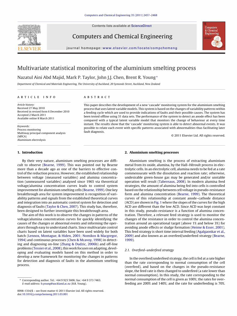
Aluminium smelting is the process of extracting aluminiummetal from its oxide, alumina, by the Hall–Héroult process in elec-trolytic cells. In an electrolytic cell, alumina needs to be fed at a ratecommensurate with the dissolution and reaction rate; otherwise,undesirable green-house gas may be generated and/or unstableoperation will result (Tabereaux, 2008). In modern alumina feedstrategies, the amount of alumina being fed into cells is controlledbased on the relationship between cell voltage in pseudo-resistanceform and alumina concentration (Bearne, 1999). The theoreticalcurves of this relationship at constant anode–cathode distance(ACD) are shown in Fig. 1 where the slopes of the curves for the highACD are different than the low ACD. Since ACD was kept constantin this study, pseudo-resistance is a function of alumina concen-tration. Therefore, a relevant feed strategy is used to monitor thechanges of the resistance in order to control the alumina concen-tration around an operational target (above 1% and below 3%) foravoiding anode effects or sludge formation (Heime & Esser, 2001).This feed strategy is short time interval feeding (Agalgaonkar et al.,2009) and also known as an overfeed/underfeed strategy (Bearne,1999).

2.1. Overfeed–underfeed strategy

In the overfeed/underfeed strategy, the cell is fed at a rate higherthan the rate corresponding to normal consumption of the cell(overfeed), and based on the changes in the pseudo-resistance

slope, the feed rate is then changed to underfeed (a rate lower thannormal consumption). In this study, the rate corresponding to thenormal consumption of the cell is given as 100%; the rates for over-feeding are 200% and 140%; and the rate for underfeeding is 70%.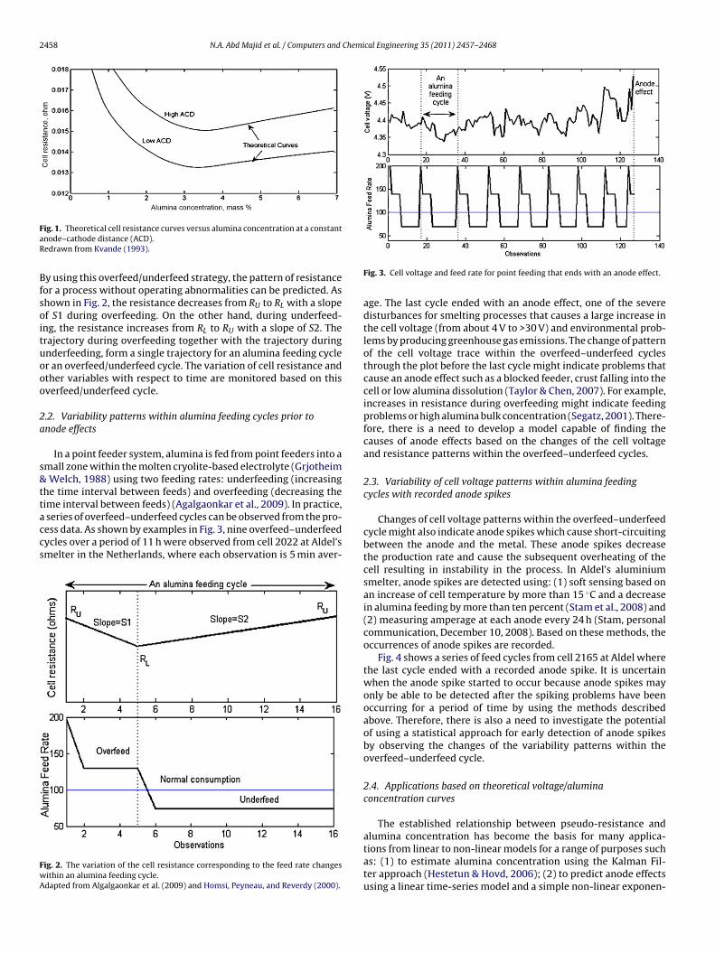

2458 N.A. Abd Majid et al. / Computers and Chemical Engineering 35 (2011) 2457– 2468

FaR

Bfsoituooo

2a

s&ttaccs

FwA

ig. 1. Theoretical cell resistance curves versus alumina concentration at a constantnode–cathode distance (ACD).edrawn from Kvande (1993).

y using this overfeed/underfeed strategy, the pattern of resistanceor a process without operating abnormalities can be predicted. Ashown in Fig. 2, the resistance decreases from RU to RL with a slopef S1 during overfeeding. On the other hand, during underfeed-ng, the resistance increases from RL to RU with a slope of S2. Therajectory during overfeeding together with the trajectory duringnderfeeding, form a single trajectory for an alumina feeding cycler an overfeed/underfeed cycle. The variation of cell resistance andther variables with respect to time are monitored based on thisverfeed/underfeed cycle.

.2. Variability patterns within alumina feeding cycles prior tonode effects

In a point feeder system, alumina is fed from point feeders into amall zone within the molten cryolite-based electrolyte (Grjotheim

Welch, 1988) using two feeding rates: underfeeding (increasinghe time interval between feeds) and overfeeding (decreasing theime interval between feeds) (Agalgaonkar et al., 2009). In practice,

series of overfeed–underfeed cycles can be observed from the pro-ess data. As shown by examples in Fig. 3, nine overfeed–underfeedycles over a period of 11 h were observed from cell 2022 at Aldel’smelter in the Netherlands, where each observation is 5 min aver-

ig. 2. The variation of the cell resistance corresponding to the feed rate changesithin an alumina feeding cycle.dapted from Algalgaonkar et al. (2009) and Homsi, Peyneau, and Reverdy (2000).

Fig. 3. Cell voltage and feed rate for point feeding that ends with an anode effect.

age. The last cycle ended with an anode effect, one of the severedisturbances for smelting processes that causes a large increase inthe cell voltage (from about 4 V to >30 V) and environmental prob-lems by producing greenhouse gas emissions. The change of patternof the cell voltage trace within the overfeed–underfeed cyclesthrough the plot before the last cycle might indicate problems thatcause an anode effect such as a blocked feeder, crust falling into thecell or low alumina dissolution (Taylor & Chen, 2007). For example,increases in resistance during overfeeding might indicate feedingproblems or high alumina bulk concentration (Segatz, 2001). There-fore, there is a need to develop a model capable of finding thecauses of anode effects based on the changes of the cell voltageand resistance patterns within the overfeed–underfeed cycles.

2.3. Variability of cell voltage patterns within alumina feedingcycles with recorded anode spikes

Changes of cell voltage patterns within the overfeed–underfeedcycle might also indicate anode spikes which cause short-circuitingbetween the anode and the metal. These anode spikes decreasethe production rate and cause the subsequent overheating of thecell resulting in instability in the process. In Aldel’s aluminiumsmelter, anode spikes are detected using: (1) soft sensing based onan increase of cell temperature by more than 15 ◦C and a decreasein alumina feeding by more than ten percent (Stam et al., 2008) and(2) measuring amperage at each anode every 24 h (Stam, personalcommunication, December 10, 2008). Based on these methods, theoccurrences of anode spikes are recorded.

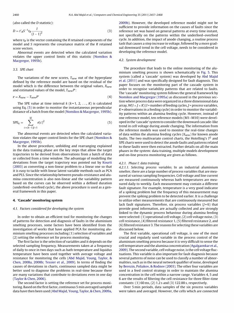
Fig. 4 shows a series of feed cycles from cell 2165 at Aldel wherethe last cycle ended with a recorded anode spike. It is uncertainwhen the anode spike started to occur because anode spikes mayonly be able to be detected after the spiking problems have beenoccurring for a period of time by using the methods describedabove. Therefore, there is also a need to investigate the potentialof using a statistical approach for early detection of anode spikesby observing the changes of the variability patterns within theoverfeed–underfeed cycle.

2.4. Applications based on theoretical voltage/aluminaconcentration curves

The established relationship between pseudo-resistance andalumina concentration has become the basis for many applica-

tions from linear to non-linear models for a range of purposes suchas: (1) to estimate alumina concentration using the Kalman Fil-ter approach (Hestetun & Hovd, 2006); (2) to predict anode effectsusing a linear time-series model and a simple non-linear exponen-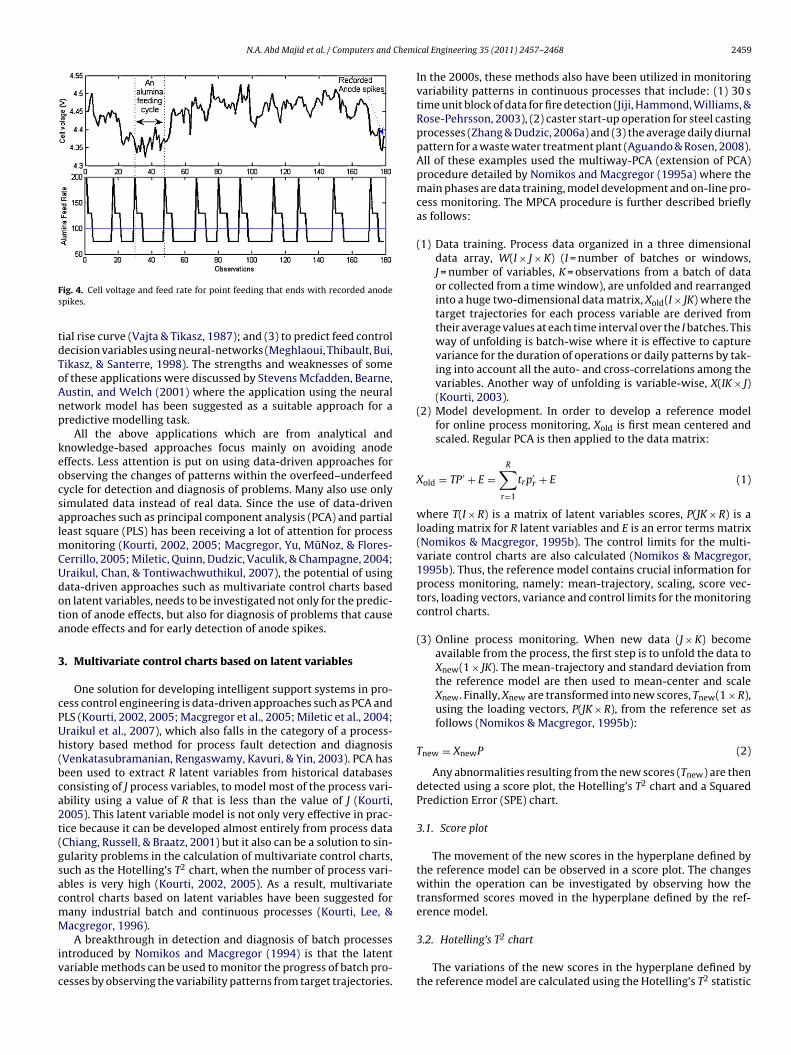

N.A. Abd Majid et al. / Computers and Chemi

Fs

tdToAnp

keocsalmCUdota

3

cPUh(bca2t(gsacmM

ivc

2

ig. 4. Cell voltage and feed rate for point feeding that ends with recorded anodepikes.

ial rise curve (Vajta & Tikasz, 1987); and (3) to predict feed controlecision variables using neural-networks (Meghlaoui, Thibault, Bui,ikasz, & Santerre, 1998). The strengths and weaknesses of somef these applications were discussed by Stevens Mcfadden, Bearne,ustin, and Welch (2001) where the application using the neuraletwork model has been suggested as a suitable approach for aredictive modelling task.

All the above applications which are from analytical andnowledge-based approaches focus mainly on avoiding anodeffects. Less attention is put on using data-driven approaches forbserving the changes of patterns within the overfeed–underfeedycle for detection and diagnosis of problems. Many also use onlyimulated data instead of real data. Since the use of data-drivenpproaches such as principal component analysis (PCA) and partialeast square (PLS) has been receiving a lot of attention for process

onitoring (Kourti, 2002, 2005; Macgregor, Yu, MuNoz, & Flores-errillo, 2005; Miletic, Quinn, Dudzic, Vaculik, & Champagne, 2004;raikul, Chan, & Tontiwachwuthikul, 2007), the potential of usingata-driven approaches such as multivariate control charts basedn latent variables, needs to be investigated not only for the predic-ion of anode effects, but also for diagnosis of problems that causenode effects and for early detection of anode spikes.

. Multivariate control charts based on latent variables

One solution for developing intelligent support systems in pro-ess control engineering is data-driven approaches such as PCA andLS (Kourti, 2002, 2005; Macgregor et al., 2005; Miletic et al., 2004;raikul et al., 2007), which also falls in the category of a process-istory based method for process fault detection and diagnosisVenkatasubramanian, Rengaswamy, Kavuri, & Yin, 2003). PCA haseen used to extract R latent variables from historical databasesonsisting of J process variables, to model most of the process vari-bility using a value of R that is less than the value of J (Kourti,005). This latent variable model is not only very effective in prac-ice because it can be developed almost entirely from process dataChiang, Russell, & Braatz, 2001) but it also can be a solution to sin-ularity problems in the calculation of multivariate control charts,uch as the Hotelling’s T2 chart, when the number of process vari-bles is very high (Kourti, 2002, 2005). As a result, multivariateontrol charts based on latent variables have been suggested forany industrial batch and continuous processes (Kourti, Lee, &acgregor, 1996).

A breakthrough in detection and diagnosis of batch processes

ntroduced by Nomikos and Macgregor (1994) is that the latentariable methods can be used to monitor the progress of batch pro-esses by observing the variability patterns from target trajectories.

cal Engineering 35 (2011) 2457– 2468 2459

In the 2000s, these methods also have been utilized in monitoringvariability patterns in continuous processes that include: (1) 30 stime unit block of data for fire detection (Jiji, Hammond, Williams, &Rose-Pehrsson, 2003), (2) caster start-up operation for steel castingprocesses (Zhang & Dudzic, 2006a) and (3) the average daily diurnalpattern for a waste water treatment plant (Aguando & Rosen, 2008).All of these examples used the multiway-PCA (extension of PCA)procedure detailed by Nomikos and Macgregor (1995a) where themain phases are data training, model development and on-line pro-cess monitoring. The MPCA procedure is further described brieflyas follows:

(1) Data training. Process data organized in a three dimensionaldata array, W(I × J × K) (I = number of batches or windows,J = number of variables, K = observations from a batch of dataor collected from a time window), are unfolded and rearrangedinto a huge two-dimensional data matrix, Xold(I × JK) where thetarget trajectories for each process variable are derived fromtheir average values at each time interval over the I batches. Thisway of unfolding is batch-wise where it is effective to capturevariance for the duration of operations or daily patterns by tak-ing into account all the auto- and cross-correlations among thevariables. Another way of unfolding is variable-wise, X(IK × J)(Kourti, 2003).

(2) Model development. In order to develop a reference modelfor online process monitoring, Xold is first mean centered andscaled. Regular PCA is then applied to the data matrix:

Xold = TP ′ + E =R∑

r=1

trp′r + E (1)

where T(I × R) is a matrix of latent variables scores, P(JK × R) is aloading matrix for R latent variables and E is an error terms matrix(Nomikos & Macgregor, 1995b). The control limits for the multi-variate control charts are also calculated (Nomikos & Macgregor,1995b). Thus, the reference model contains crucial information forprocess monitoring, namely: mean-trajectory, scaling, score vec-tors, loading vectors, variance and control limits for the monitoringcontrol charts.

(3) Online process monitoring. When new data (J × K) becomeavailable from the process, the first step is to unfold the data toXnew(1 × JK). The mean-trajectory and standard deviation fromthe reference model are then used to mean-center and scaleXnew. Finally, Xnew are transformed into new scores, Tnew(1 × R),using the loading vectors, P(JK × R), from the reference set asfollows (Nomikos & Macgregor, 1995b):

Tnew = XnewP (2)

Any abnormalities resulting from the new scores (Tnew) are thendetected using a score plot, the Hotelling’s T2 chart and a SquaredPrediction Error (SPE) chart.

3.1. Score plot

The movement of the new scores in the hyperplane defined bythe reference model can be observed in a score plot. The changeswithin the operation can be investigated by observing how thetransformed scores moved in the hyperplane defined by the ref-erence model.

3.2. Hotelling’s T chart

The variations of the new scores in the hyperplane defined bythe reference model are calculated using the Hotelling’s T2 statistic

2 Chemi

(

D

wms

vM

3

dma

e

ud

S

tM

itod(iamb(e

4

4

osim(

sotrCcba(

td

460 N.A. Abd Majid et al. / Computers and

also called the D statistic):

= t′RS−1tR

I

(I − 1)2(3)

here tR is the vector containing the R retained components of theodel and S represents the covariance matrix of the R retained

core vectors.Abnormal events are detected when the calculated variation

iolates the upper control limits of this statistic (Nomikos &acgregor, 1995b).

.3. SPE chart

The variations of the new scores, Tnew out of the hyperplaneefined by the reference model are based on the residual of theodel which is the difference between the original values, Xnew

nd estimated values of the model, TnewP′:

= Xnew − TnewP ′ (4)

The SPE value at time interval k (k = 1, 2, . . ., K) is calculatedsing Eq. (5) in order to monitor the instantaneous perpendicularistance of a batch from the model (Nomikos & Macgregor, 1995b).

PEk =kJ∑

c=(k−1)J+1

e(c)2 (5)

The abnormal events are detected when the calculated varia-ion violates the upper control limits for the SPE chart (Nomikos &

acgregor, 1995b).In the above procedure, unfolding and rearranging explained

n the data training phase are the key steps that allow the targetrajectories to be derived from observations from a batch of datar collected from a time window. The advantage of modelling theeviations from the target trajectory was pointed out by Kourti2003) as converting a non-linear problem to a linear one so thatt is easy to tackle with linear latent variable methods such as PCAnd PLS. Since the relationship between pseudo-resistance and alu-ina concentration is also non-linear and the variability pattern

ased on the curves can be observed within a defined durationunderfeed–overfeed cycle), the above procedure is used as a gen-ral framework in this paper.

. ‘Cascade’ monitoring system

.1. Factors considered for developing the system

In order to obtain an efficient tool for monitoring the changesf patterns for detection and diagnosis of faults in the aluminiummelting processes, some factors have been identified from thenvestigation of works that have applied PCA for monitoring alu-

inium smelting processes including (1) selection of variables and2) setting the reference set for process monitoring.

The first factor is the selection of variables and it depends on theelected sampling frequency. Measurements taken at a frequencyf daily to once in two days such as bath temperature and liquidusemperature have been used together with average voltage andesistance for monitoring the cells (Abd Majid, Young, Taylor, &hen, 2008a, 2008b; Tessier et al., 2009). In terms of finding theauses of deviations in charts, continuous sampled data might beetter used to diagnose the problems in real-time because therere many variations that contribute to deviations even in one day

Taylor & Chen, 2006).

The second factor is setting the reference set for process moni-oring. Based on the first factor, continuous 5 min averaged sampledata have then been used (Abd Majid, Young, Taylor, & Chen, 2009a,

cal Engineering 35 (2011) 2457– 2468

2009b). However, the developed reference model might not besufficient to provide information on the causes of faults since thereference set was based on general patterns at every time instant,not specifically on the patterns within the underfeed–overfeedcycle. In addition, the impact of anode changing, a routine processtask that causes a step increase in voltage, followed by a more grad-ual downward trend in the cell voltage, needs to be considered indeveloping the reference model.

4.2. System development

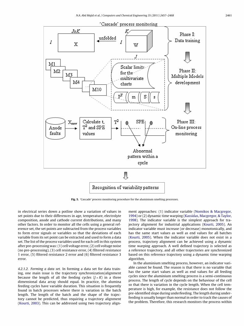
The procedure that leads to the online monitoring of the alu-minium smelting process is shown schematically in Fig. 5. Thissystem (called a ‘cascade’ system) was developed by Abd Majidet al. (2011) and was specifically designed for fault diagnosis. Thispaper focuses on the monitoring part of the cascade system inorder to recognise variability patterns that are related to faults.The ‘cascade’ monitoring system follows the general framework byNomikos and Macgregor (1995a) as discussed in the previous sec-tion where process data were organized in a three dimensional dataarray, W(I × J × K) (I = number of feeding cycles, J = process variables,K = observations in a feeding cycle) in order to monitor the variabil-ity patterns within an alumina feeding cycle. However, instead ofone reference model, ten reference models (M1–M10) were devel-oped in the ‘cascade’ system to consider the downward cascade-liketrend in cell voltage during anode changing. The information fromthe reference models was used to monitor the real-time changesof data within the alumina feeding cycles (Xnew) for known anodefaults. The two multivariate control charts, the Hotelling’s T2 andSPE charts were used to detect the anode faults and patterns relatedto these faults were then extracted. Further details on all the mainphases in the system: data training, multiple models developmentand on-line process monitoring are given as follows.

4.2.1. Phase I: data training4.2.1.1. Selecting process variables. In an industrial aluminiumsmelter, there are a large number of process variables that are mea-sured at various sampling frequencies. Cell voltage and line currentare measured continuously whereas bath temperatures are mea-sured daily to weekly. Each measurement may contain a differentfault signature. For example, temperature is a very good indicatorof a spiking problem but the frequency of this measurement mayprevent the spiking problem to be detected earlier. It is a challengeto utilize other measurements that are continuously measured butlack fault signatures. Therefore, six process variables (J = 6) thatprovide good information, are actually collected and are stronglylinked to the dynamic process behaviour during alumina feedingwere selected: (1) operational cell voltage, (2) cell voltage noise, (3)cell resistance, (4) filtered resistance 1, (5) filtered resistance 2, and(6) filtered resistance 3. The reasons for selecting these variables arediscussed below.

The first variable, operational cell voltage, is one of the mostcrucial and regularly used variable in the process control of thealuminium smelting process because it is very difficult to sense thecell temperature and the alumina concentration (Agalgaonkar et al.,2009). The second variable, cell voltage noise, is the cell voltage fluc-tuations. This variable is also important for fault diagnosis becauseseveral patterns of noise can be used to classify a number of abnor-malities, such as in the neural network qualifier of noise, developedby Berezin, Poliakov, & Rodnov (2003). The other four variables areused in a feed control strategy in order to maintain the aluminaconcentration in the cell within a narrow range. Variables 4, 5 and

6 are the results of filtering the cell resistance for three filter-timeconstants: (1) 60 ms, (2) 1.2 s and (3) 122.88 s, respectively.

Over 5 min periods, data samples of the six process variableswere taken and averaged. However, the cells which are connected

N.A. Abd Majid et al. / Computers and Chemical Engineering 35 (2011) 2457– 2468 2461

cedur

iscoetvsa(1e

4ibdfflt(

Fig. 5. ‘Cascade’ process monitoring pro

n electrical series down a potline show a variation of values inet points due to their differences in age, temperature, electrolyteomposition, anode and cathode current distributions, and manyther factors. In order to monitor all the cells using a general ref-rence set, the set points are subtracted from the process variableso form error signals or variables so that the deviations of eachariable from its set point can be extracted and used to form a dataet. The list of the process variables used for each cell in this systemfter pre-processing was: (1) cell voltage error, (2) cell voltage noiseno pre-processing), (3) cell resistance error, (4) filtered resistance

error, (5) filtered resistance 2 error and (6) filtered resistance 3rror.

.2.1.2. Forming a data set. In forming a data set for data train-ng, one main issue is the trajectory synchronization/alignmentecause the length of all the feeding cycles (J × K) in a threeimensional data array should equal. In practice, the aluminaeeding cycles have variable duration. This situation is frequently

ound in batch processes where there is variation in the batchength. The length of the batch and the shape of the trajec-ory cannot be predicted, thus requiring a trajectory alignmentKourti, 2003). This can be addressed using two trajectory align-

e for the aluminium smelting processes.

ment approaches: (1) indicator variable (Nomikos & Macgregor,1994) or (2) dynamic time warping (Kassidas, Macgregor, & Taylor,1998). The indicator variable is the simplest approach for tra-jectory alignment for industrial applications (Kourti, 2005). Anindicator variable must increase (or decrease) monotonically, andhas the same start values as well as end values for all batches(Kourti, 2005). When the indicator variable does not exist in aprocess, trajectory alignment can be achieved using a dynamictime warping approach. A well defined trajectory is selected asa reference trajectory, and all other trajectories are synchronizedbased on this reference trajectory using a dynamic time warpingalgorithm.

In the aluminium smelting process, however, an indicator vari-able cannot be found. The reason is that there is no variable thathas the same start values as well as end values for all feedingcycles since the aluminium smelting process is a semi-continuousprocess. The length of cycle depends on the behaviour of the cellso that there is variation in the cycle length. When the cell tem-

perature is high, for example, the resistance does not follow thepre-identified slope during underfeeding. The length during under-feeding is usually longer than normal in order to track the causes ofthe problem. Therefore, this research monitors the process within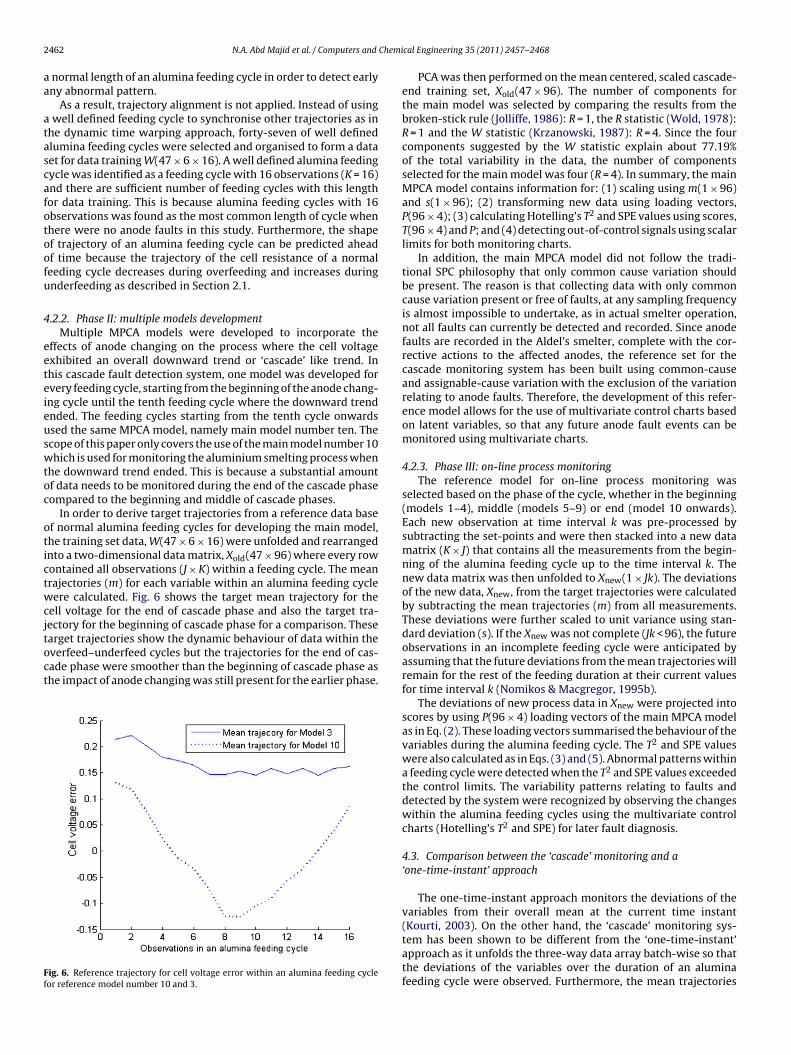

2 Chemi

aa

atascafotoofu

4

eeteieuswtoc

otictwcjtoct

Ff

462 N.A. Abd Majid et al. / Computers and

normal length of an alumina feeding cycle in order to detect earlyny abnormal pattern.

As a result, trajectory alignment is not applied. Instead of using well defined feeding cycle to synchronise other trajectories as inhe dynamic time warping approach, forty-seven of well definedlumina feeding cycles were selected and organised to form a dataet for data training W(47 × 6 × 16). A well defined alumina feedingycle was identified as a feeding cycle with 16 observations (K = 16)nd there are sufficient number of feeding cycles with this lengthor data training. This is because alumina feeding cycles with 16bservations was found as the most common length of cycle whenhere were no anode faults in this study. Furthermore, the shapef trajectory of an alumina feeding cycle can be predicted aheadf time because the trajectory of the cell resistance of a normaleeding cycle decreases during overfeeding and increases duringnderfeeding as described in Section 2.1.

.2.2. Phase II: multiple models developmentMultiple MPCA models were developed to incorporate the

ffects of anode changing on the process where the cell voltagexhibited an overall downward trend or ‘cascade’ like trend. Inhis cascade fault detection system, one model was developed forvery feeding cycle, starting from the beginning of the anode chang-ng cycle until the tenth feeding cycle where the downward trendnded. The feeding cycles starting from the tenth cycle onwardssed the same MPCA model, namely main model number ten. Thecope of this paper only covers the use of the main model number 10hich is used for monitoring the aluminium smelting process when

he downward trend ended. This is because a substantial amountf data needs to be monitored during the end of the cascade phaseompared to the beginning and middle of cascade phases.

In order to derive target trajectories from a reference data basef normal alumina feeding cycles for developing the main model,he training set data, W(47 × 6 × 16) were unfolded and rearrangednto a two-dimensional data matrix, Xold(47 × 96) where every rowontained all observations (J × K) within a feeding cycle. The meanrajectories (m) for each variable within an alumina feeding cycleere calculated. Fig. 6 shows the target mean trajectory for the

ell voltage for the end of cascade phase and also the target tra-ectory for the beginning of cascade phase for a comparison. Thesearget trajectories show the dynamic behaviour of data within the

verfeed–underfeed cycles but the trajectories for the end of cas-ade phase were smoother than the beginning of cascade phase ashe impact of anode changing was still present for the earlier phase.

ig. 6. Reference trajectory for cell voltage error within an alumina feeding cycleor reference model number 10 and 3.

cal Engineering 35 (2011) 2457– 2468

PCA was then performed on the mean centered, scaled cascade-end training set, Xold(47 × 96). The number of components forthe main model was selected by comparing the results from thebroken-stick rule (Jolliffe, 1986): R = 1, the R statistic (Wold, 1978):R = 1 and the W statistic (Krzanowski, 1987): R = 4. Since the fourcomponents suggested by the W statistic explain about 77.19%of the total variability in the data, the number of componentsselected for the main model was four (R = 4). In summary, the mainMPCA model contains information for: (1) scaling using m(1 × 96)and s(1 × 96); (2) transforming new data using loading vectors,P(96 × 4); (3) calculating Hotelling’s T2 and SPE values using scores,T(96 × 4) and P; and (4) detecting out-of-control signals using scalarlimits for both monitoring charts.

In addition, the main MPCA model did not follow the tradi-tional SPC philosophy that only common cause variation shouldbe present. The reason is that collecting data with only commoncause variation present or free of faults, at any sampling frequencyis almost impossible to undertake, as in actual smelter operation,not all faults can currently be detected and recorded. Since anodefaults are recorded in the Aldel’s smelter, complete with the cor-rective actions to the affected anodes, the reference set for thecascade monitoring system has been built using common-causeand assignable-cause variation with the exclusion of the variationrelating to anode faults. Therefore, the development of this refer-ence model allows for the use of multivariate control charts basedon latent variables, so that any future anode fault events can bemonitored using multivariate charts.

4.2.3. Phase III: on-line process monitoringThe reference model for on-line process monitoring was

selected based on the phase of the cycle, whether in the beginning(models 1–4), middle (models 5–9) or end (model 10 onwards).Each new observation at time interval k was pre-processed bysubtracting the set-points and were then stacked into a new datamatrix (K × J) that contains all the measurements from the begin-ning of the alumina feeding cycle up to the time interval k. Thenew data matrix was then unfolded to Xnew(1 × Jk). The deviationsof the new data, Xnew, from the target trajectories were calculatedby subtracting the mean trajectories (m) from all measurements.These deviations were further scaled to unit variance using stan-dard deviation (s). If the Xnew was not complete (Jk < 96), the futureobservations in an incomplete feeding cycle were anticipated byassuming that the future deviations from the mean trajectories willremain for the rest of the feeding duration at their current valuesfor time interval k (Nomikos & Macgregor, 1995b).

The deviations of new process data in Xnew were projected intoscores by using P(96 × 4) loading vectors of the main MPCA modelas in Eq. (2). These loading vectors summarised the behaviour of thevariables during the alumina feeding cycle. The T2 and SPE valueswere also calculated as in Eqs. (3) and (5). Abnormal patterns withina feeding cycle were detected when the T2 and SPE values exceededthe control limits. The variability patterns relating to faults anddetected by the system were recognized by observing the changeswithin the alumina feeding cycles using the multivariate controlcharts (Hotelling’s T2 and SPE) for later fault diagnosis.

4.3. Comparison between the ‘cascade’ monitoring and a‘one-time-instant’ approach

The one-time-instant approach monitors the deviations of thevariables from their overall mean at the current time instant(Kourti, 2003). On the other hand, the ‘cascade’ monitoring sys-

tem has been shown to be different from the ‘one-time-instant’approach as it unfolds the three-way data array batch-wise so thatthe deviations of the variables over the duration of an aluminafeeding cycle were observed. Furthermore, the mean trajectories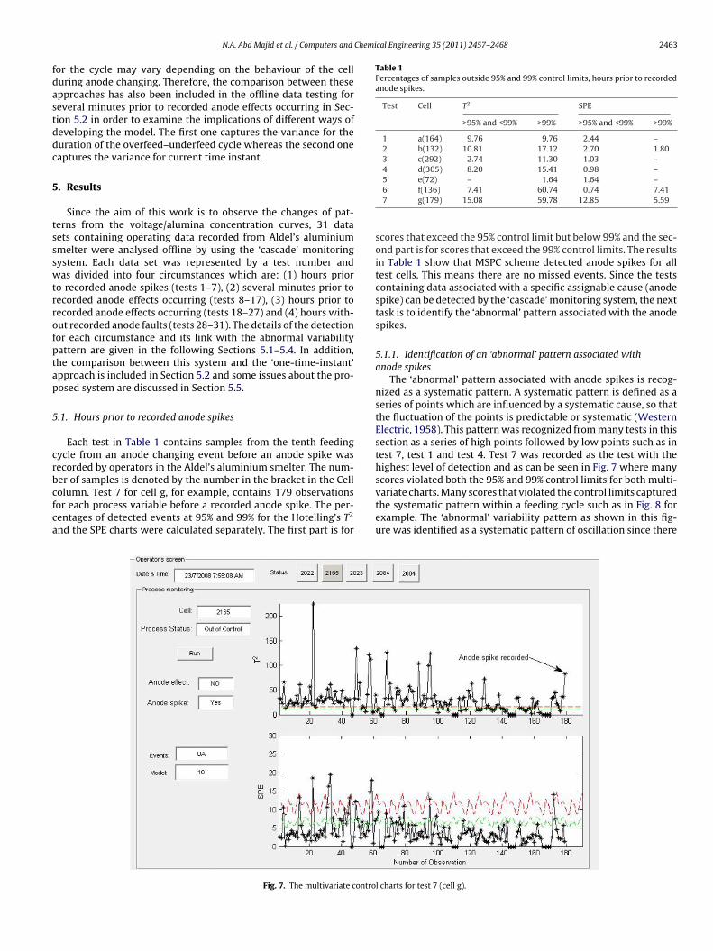

Chemical Engineering 35 (2011) 2457– 2468 2463

fdastddc

5

tssswtrrofptap

5

crbcfca

Table 1Percentages of samples outside 95% and 99% control limits, hours prior to recordedanode spikes.

Test Cell T2 SPE

>95% and <99% >99% >95% and <99% >99%

1 a(164) 9.76 9.76 2.44 –2 b(132) 10.81 17.12 2.70 1.803 c(292) 2.74 11.30 1.03 –4 d(305) 8.20 15.41 0.98 –5 e(72) – 1.64 1.64 –

N.A. Abd Majid et al. / Computers and

or the cycle may vary depending on the behaviour of the celluring anode changing. Therefore, the comparison between thesepproaches has also been included in the offline data testing foreveral minutes prior to recorded anode effects occurring in Sec-ion 5.2 in order to examine the implications of different ways ofeveloping the model. The first one captures the variance for theuration of the overfeed–underfeed cycle whereas the second oneaptures the variance for current time instant.

. Results

Since the aim of this work is to observe the changes of pat-erns from the voltage/alumina concentration curves, 31 dataets containing operating data recorded from Aldel’s aluminiummelter were analysed offline by using the ‘cascade’ monitoringystem. Each data set was represented by a test number andas divided into four circumstances which are: (1) hours prior

o recorded anode spikes (tests 1–7), (2) several minutes prior toecorded anode effects occurring (tests 8–17), (3) hours prior toecorded anode effects occurring (tests 18–27) and (4) hours with-ut recorded anode faults (tests 28–31). The details of the detectionor each circumstance and its link with the abnormal variabilityattern are given in the following Sections 5.1–5.4. In addition,he comparison between this system and the ‘one-time-instant’pproach is included in Section 5.2 and some issues about the pro-osed system are discussed in Section 5.5.

.1. Hours prior to recorded anode spikes

Each test in Table 1 contains samples from the tenth feedingycle from an anode changing event before an anode spike wasecorded by operators in the Aldel’s aluminium smelter. The num-er of samples is denoted by the number in the bracket in the Cell

olumn. Test 7 for cell g, for example, contains 179 observationsor each process variable before a recorded anode spike. The per-entages of detected events at 95% and 99% for the Hotelling’s T2

nd the SPE charts were calculated separately. The first part is for

Fig. 7. The multivariate contro

6 f(136) 7.41 60.74 0.74 7.417 g(179) 15.08 59.78 12.85 5.59

scores that exceed the 95% control limit but below 99% and the sec-ond part is for scores that exceed the 99% control limits. The resultsin Table 1 show that MSPC scheme detected anode spikes for alltest cells. This means there are no missed events. Since the testscontaining data associated with a specific assignable cause (anodespike) can be detected by the ‘cascade’ monitoring system, the nexttask is to identify the ‘abnormal’ pattern associated with the anodespikes.

5.1.1. Identification of an ‘abnormal’ pattern associated withanode spikes

The ‘abnormal’ pattern associated with anode spikes is recog-nized as a systematic pattern. A systematic pattern is defined as aseries of points which are influenced by a systematic cause, so thatthe fluctuation of the points is predictable or systematic (WesternElectric, 1958). This pattern was recognized from many tests in thissection as a series of high points followed by low points such as intest 7, test 1 and test 4. Test 7 was recorded as the test with thehighest level of detection and as can be seen in Fig. 7 where manyscores violated both the 95% and 99% control limits for both multi-

variate charts. Many scores that violated the control limits capturedthe systematic pattern within a feeding cycle such as in Fig. 8 forexample. The ‘abnormal’ variability pattern as shown in this fig-ure was identified as a systematic pattern of oscillation since there

l charts for test 7 (cell g).

2464 N.A. Abd Majid et al. / Computers and Chemical Engineering 35 (2011) 2457– 2468

apoapsdt

5

tTdoecw

Table 2Percentages of samples outside 95% and 99% control limits, within 20 min prior toanode effect occurring.

Test Cell T2 SPE

>95% and <99% >99% >95% and <99% >99%

8 h(167–170) – 25 – –9 i(377–380) – 25 – 25

10 j(117–120) – 25 – 2511 k(100–103) – 100 – –12 l(50–53) – 100 50 2513 o(125–127) – 100 – 7514 p(131–134) – 75 – 5015 q(423–426) 75 – – –

Fig. 8. Part of the variability pattern for score 47 in test 7.

re high points was followed by low points. The same oscillatoryattern was also observed from other tests. For example, this wasbserved hours before a recorded anode spike for cell a (test 1)nd cell d (test 4). This systematic pattern can be linked to spikingroblems since it was happening hours before the recorded anodepike. It also shows the influence of the spiking problems on theata as the problems occur when an extension from an anode hitshe metal and consequently affects the cell voltage.

.2. Several minutes prior to anode effects occurring

The MSPC scheme detected anode effects several minutes beforehe anode effects occurring for all test cells as given in detail inable 2 so that there were no missed events. However, there areifferences in the percentage of detection depend on the magnitude

f changes in the ‘abnormal’ variability pattern prior to the anodeffect occurring. For test 17, for example, only one score violated theontrol limits and this might be because the typical task, tapping,as done in a few minutes before the anode effect happened.

Fig. 9. Evidence of control limits violations in the multivariate c

16 r(307–310) – 50 25 2517 s(255–258) 25 – – –

5.2.1. Identification of an ‘abnormal’ pattern associated withanode effects

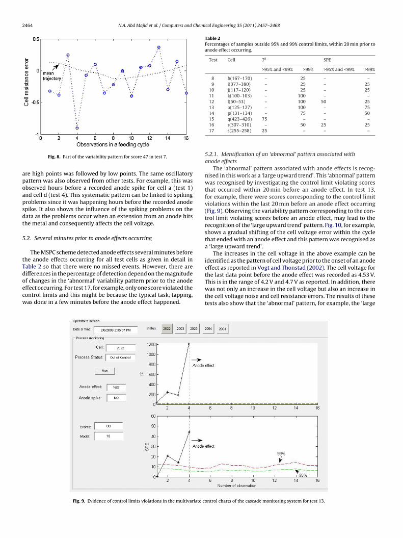
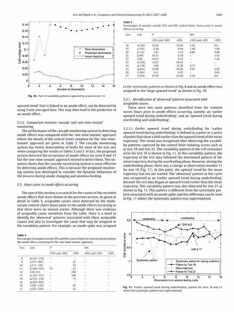
The ‘abnormal’ pattern associated with anode effects is recog-nised in this work as a ‘large upward trend’. This ‘abnormal’ patternwas recognised by investigating the control limit violating scoresthat occurred within 20 min before an anode effect. In test 13,for example, there were scores corresponding to the control limitviolations within the last 20 min before an anode effect occurring(Fig. 9). Observing the variability pattern corresponding to the con-trol limit violating scores before an anode effect, may lead to therecognition of the ‘large upward trend’ pattern. Fig. 10, for example,shows a gradual shifting of the cell voltage error within the cyclethat ended with an anode effect and this pattern was recognised asa ‘large upward trend’.

The increases in the cell voltage in the above example can beidentified as the pattern of cell voltage prior to the onset of an anodeeffect as reported in Vogt and Thonstad (2002). The cell voltage forthe last data point before the anode effect was recorded as 4.53 V.This is in the range of 4.2 V and 4.7 V as reported. In addition, there

was not only an increase in the cell voltage but also an increase inthe cell voltage noise and cell resistance errors. The results of thesetests also show that the ‘abnormal’ pattern, for example, the ‘large

ontrol charts of the cascade monitoring system for test 13.

N.A. Abd Majid et al. / Computers and Chemical Engineering 35 (2011) 2457– 2468 2465

uua

5m

awiswsbufit

5

advtoict

TPt

Table 4Percentages of samples outside 95% and 99% control limits, hours prior to anodeeffects occurring.

Test Cell T2 SPE

>95% and <99% >99% >95% and <99% >99%

18 h(166) 10.30 23.64 2.42 0.619 i(376) 4.26 9.04 1.06 1.0620 j(116) 3.45 3.45 0.86 0.8621 k(99) 16.33 9.18 – 1.0222 l(49) 16.33 9.18 – 1.0223 o(124) 13.82 50.41 – –24 p(130) 3.84 15.38 0.77 –25 q(422) 15.09 28.30 0.47 2.83

shown in Fig. 11. This pattern is different from the systematic pat-tern associated with an anode spike and this difference can be seenin Fig. 11 where the systematic pattern was superimposed.

Fig. 10. Part of variability patterns captured by scores in test 13.

pward trend’ that is linked to an anode effect, can be detected bysing 5 min averaged data. This may then lead to the prediction ofn anode effect.

.2.2. Comparison between ‘cascade’ and ‘one-time-instant’onitoring

The performance of the cascade monitoring system in detectingnode effects was compared with the ‘one-time-instant’ approachhere the details of the control limits violation for the ‘one-time-

nstant’ approach are given in Table 3. The cascade monitoringystem has better detectability of faults for most of the test setshen comparing the results in Tables 2 and 3. In fact, the proposed

ystem detected the occurrence of anode effects for tests 8 and 15ut the ‘one-time-instant’ approach missed to detect them. This sit-ation shows that the cascade monitoring system is more effectiveor detecting anode effects. This is because the proposed monitor-ng system was developed to consider the dynamic behaviour ofhe process during anode changing and alumina feeding.

.3. Hours prior to anode effects occurring

The aim of this section is to search for the causes of the recordednode effects that were shown in the previous section. As given inetail in Table 4, assignable causes were detected by the multi-ariate control charts hours prior to the anode effects occurring sohat there were no missed events. Although there was evidence

f assignable cause variations from the table, there is a need todentify the ‘abnormal’ patterns associated with these assignableauses and also to investigate the cause that may be assigned tohe variability pattern. For example, an anode spike was assigned

able 3ercentages of samples outside 95% and 99% control limits for several minutes beforehe anode effects occurring for the ‘one-time-instant’ approach.

Test Cell T2 SPE

>95% and <99% >99% >95% and <99% >99%

8 h(167–170) – – – –9 i(377–380) – 25 – –

10 j(117–120) – 25 – –11 k(100–103) 75 25 – –12 l(50–53) – 100 – –13 o(125–127) – 100 – –14 p(131–134) – 75 – –15 q(423–426) – – – –16 r(307–310) – 50 – –17 s(255–258) – 25 – –

26 r(306) 2.61 4.25 – 0.6527 s(254) 10.30 23.64 2.42 0.6

to the systematic pattern as shown in Fig. 8 and an anode effect wasassigned to the ‘large upward trend’ as shown in Fig. 10.

5.3.1. Identification of ‘abnormal’ patterns associated withassignable causes

There were two main patterns identified from the violatedscores hours prior to anode effects occurring, namely: an ‘earlierupward trend during underfeeding’; and an ‘upward trend duringoverfeeding and underfeeding’.

5.3.1.1. Earlier upward trend during underfeeding. An ‘earlierupward trend during underfeeding’ is defined as a point or a seriesof points that show a shift earlier than the upward trend of the meantrajectory. This trend was recognised after observing the variabil-ity patterns captured by the control limit violating scores such asin test 18 and test 21. The variability pattern of the cell resistanceerror for test 18 is shown in Fig. 11. In this variability pattern, thetrajectory of the test data followed the downward pattern of themean trajectory during the overfeeding phase. However, during theunderfeeding phase, there was a change at observation number 11for test 18 (Fig. 11). At this point, the upward trend for the meantrajectory had not yet started. The ‘abnormal’ pattern in this cyclewas recognised as an ‘earlier upward trend during underfeeding’because the test data began an upward trend earlier than the meantrajectory. This variability pattern was also observed for test 21 as

Fig. 11. ‘Earlier upward trend during underfeeding’ pattern for tests 18 and 21where the systematic pattern was superimposed.

2466 N.A. Abd Majid et al. / Computers and Chemi

F2

5‘ooTc2ldf

5c

httTlu

5ebmapcasaihS

tTwtTceaP

address this problem. This is based on the fact that the set pointsare actually the target ACD. After pre-processing, process data wererecorded as deviation variables from their set points before thereference model development. Furthermore, the differences in age

Table 5Percentages of samples outside 95% and 99% control limits, hours without recordedanode faults.

Test Cell T2 SPE

>95% and <99% >99% >95% and <99% >99%

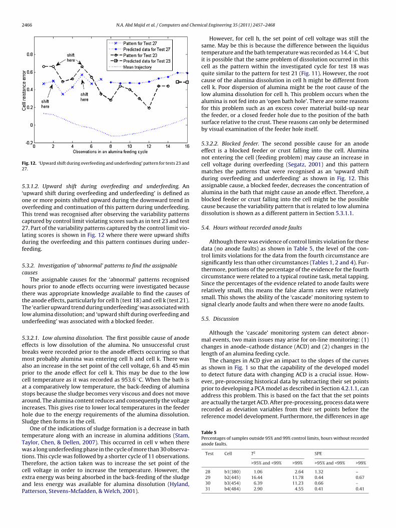
ig. 12. ‘Upward shift during overfeeding and underfeeding’ pattern for tests 23 and7.

.3.1.2. Upward shift during overfeeding and underfeeding. Anupward shift during overfeeding and underfeeding’ is defined asne or more points shifted upward during the downward trend inverfeeding and continuation of this pattern during underfeeding.his trend was recognised after observing the variability patternsaptured by control limit violating scores such as in test 23 and test7. Part of the variability patterns captured by the control limit vio-

ating scores is shown in Fig. 12 where there were upward shiftsuring the overfeeding and this pattern continues during under-eeding.

.3.2. Investigation of ‘abnormal’ patterns to find the assignableauses

The assignable causes for the ‘abnormal’ patterns recognisedours prior to anode effects occurring were investigated becausehere was appropriate knowledge available to find the causes ofhe anode effects, particularly for cell h (test 18) and cell k (test 21).he ‘earlier upward trend during underfeeding’ was associated withow alumina dissolution; and ‘upward shift during overfeeding andnderfeeding’ was associated with a blocked feeder.

.3.2.1. Low alumina dissolution. The first possible cause of anodeffects is low dissolution of the alumina. No unsuccessful crustreaks were recorded prior to the anode effects occurring so thatost probably alumina was entering cell h and cell k. There was

lso an increase in the set point of the cell voltage, 6 h and 45 minrior to the anode effect for cell k. This may be due to the lowell temperature as it was recorded as 953.6 ◦C. When the bath ist a comparatively low temperature, the back-feeding of aluminatops because the sludge becomes very viscous and does not moveround. The alumina content reduces and consequently the voltagencreases. This gives rise to lower local temperatures in the feederole due to the energy requirements of the alumina dissolution.ludge then forms in the cell.

One of the indications of sludge formation is a decrease in bathemperature along with an increase in alumina additions (Stam,aylor, Chen, & Dellen, 2007). This occurred in cell v when thereas a long underfeeding phase in the cycle of more than 30 observa-

ions. This cycle was followed by a shorter cycle of 11 observations.herefore, the action taken was to increase the set point of the

ell voltage in order to increase the temperature. However, thextra energy was being absorbed in the back-feeding of the sludgend less energy was available for alumina dissolution (Hyland,atterson, Stevens-Mcfadden, & Welch, 2001).

cal Engineering 35 (2011) 2457– 2468

However, for cell h, the set point of cell voltage was still thesame. May be this is because the difference between the liquidustemperature and the bath temperature was recorded as 14.4 ◦C, butit is possible that the same problem of dissolution occurred in thiscell as the pattern within the investigated cycle for test 18 wasquite similar to the pattern for test 21 (Fig. 11). However, the rootcause of the alumina dissolution in cell h might be different fromcell k. Poor dispersion of alumina might be the root cause of thelow alumina dissolution for cell h. This problem occurs when thealumina is not fed into an ‘open bath hole’. There are some reasonsfor this problem such as an excess cover material build-up nearthe feeder, or a closed feeder hole due to the position of the bathsurface relative to the crust. These reasons can only be determinedby visual examination of the feeder hole itself.

5.3.2.2. Blocked feeder. The second possible cause for an anodeeffect is a blocked feeder or crust falling into the cell. Aluminanot entering the cell (feeding problem) may cause an increase incell voltage during overfeeding (Segatz, 2001) and this patternmatches the patterns that were recognised as an ‘upward shiftduring overfeeding and underfeeding’ as shown in Fig. 12. Thisassignable cause, a blocked feeder, decreases the concentration ofalumina in the bath that might cause an anode effect. Therefore, ablocked feeder or crust falling into the cell might be the possiblecause because the variability pattern that is related to low aluminadissolution is shown as a different pattern in Section 5.3.1.1.

5.4. Hours without recorded anode faults

Although there was evidence of control limits violation for thesedata (no anode faults) as shown in Table 5, the level of the con-trol limits violations for the data from the fourth circumstance aresignificantly less than other circumstances (Tables 1, 2 and 4). Fur-thermore, portions of the percentage of the evidence for the fourthcircumstance were related to a typical routine task, metal tapping.Since the percentages of the evidence related to anode faults wererelatively small, this means the false alarm rates were relativelysmall. This shows the ability of the ‘cascade’ monitoring system tosignal clearly anode faults and when there were no anode faults.

5.5. Discussion

Although the ‘cascade’ monitoring system can detect abnor-mal events, two main issues may arise for on-line monitoring: (1)changes in anode–cathode distance (ACD) and (2) changes in thelength of an alumina feeding cycle.

The changes in ACD give an impact to the slopes of the curvesas shown in Fig. 1 so that the capability of the developed modelto detect future data with changing ACD is a crucial issue. How-ever, pre-processing historical data by subtracting their set pointsprior to developing a PCA model as described in Section 4.2.1.1, can

28 b1(380) 1.06 2.64 1.32 –29 b2(445) 16.44 11.78 0.44 0.6730 b3(454) 6.39 11.23 0.66 –31 b4(484) 2.90 4.55 0.41 0.41

Chemi

adrtrftnpod

woctdiHtbTfbfbtcen

6

cs

(

(

covf

A

Aa

N.A. Abd Majid et al. / Computers and

nd temperature of the cells were also removed by monitoring theeviation of the process from its current state which is at its cur-ent set point. For example, when the set point of cell voltage forhe new data is increased because of the low bath temperature, theeference model from the cascade monitoring system is still validor monitoring the new data because their set points will be sub-racted. Thus, the reference model can be used for monitoring aumber of cells and at different periods of plant operation. To sup-ort this, and by way of validation, the recorded faults used in theffline data testing were from different cells and were also fromifferent periods of plant operation.

Since the proposed system monitors the variability patternithin an alumina feeding cycle with 16 observations, the length

f a new alumina feeding cycle which is more than 16 observationsauses the system to stop monitoring until another new cycle. Inhis situation, a typical PCA model can be developed to monitorata that are recorded beyond the length of the normal cycle since

t is not based on the dynamic behaviour during alumina feeding.owever, the use of the ‘cascade’ monitoring system is adequate

o detect early faults since the abnormal pattern was observedased on the pre-identified curve during a normal feeding cycle.his means although only 16 observations were monitored for eacheeding cycle, the proposed variability patterns can be detectedased on the changing of patterns during overfeeding or under-eeding. The cycle duration can be added as a separate variable toe monitored together with cell temperature, liquidus tempera-ure and excess AlF3. These three variables can assist in finding theauses of problem but were not included in the developed refer-nce model since they are measured only once every two days andot online.

. Summary and conclusions

The changes of patterns in the voltage/alumina concentrationurves were observed from 31 data sets by the ‘cascade’ monitoringystem and the results show:

(a) The use of the ‘cascade’ monitoring system leads to early detec-tion of an anode spike, prediction of an anode effect and also tothe detections of problems that may have caused anode effects.

b) Four ‘abnormal’ patterns were recognised to be associated withfour different events: (1) a systematic pattern for an anodespike, (2) a ‘large upward trend’ for prediction of an anodeeffect, (3) an ‘earlier upward trend during underfeeding’ for lowalumina dissolution and (4) an ‘upward shift during overfeedingand underfeeding’ for the occurrence of a blocked feeder.

(c) The reference model for detecting anode faults was constructedby using data from a range of cells and from a range of differ-ent periods but the spiking problems recorded later and fromdifferent cells was able to be detected by the developed model.

d) The development of the reference model with common causeand assignable cause variation appears to be an alternativesolution for developing a data-based monitoring system forcomplex processes such as the aluminium electrolysis process.

All in all, the ‘cascade’ monitoring system appears to be an effi-ient tool for monitoring the changes of patterns for the detectionf faults in the aluminium smelting process. The recognition of theariability patterns would provide information for developing aault diagnosis as part of this ‘cascade’ monitoring system.

cknowledgments

Thanks to Marco Stam and Albert Mulder, and their companyldel for providing the data and assisting by answering the firstuthor’s questions on operational activities. The first author also

cal Engineering 35 (2011) 2457– 2468 2467

acknowledges the financial support of the Ministry of Higher Edu-cation of Malaysia and the National University of Malaysia.

References

Abd Majid, N. A., Young, B., Taylor, M. P., & Chen, J. J. J. (2008a). PCA-based pro-cess monitoring and fault diagnosis for aluminium processing. In Internationalconference on mechanical & manufacturing engineering (ICME2008) Johore Bahru,Malaysia.

Abd Majid, N. A., Young, B., Taylor, M. P., & Chen, J. J. J. (2008b). Real-time processmonitoring and fault diagnosis for aluminium processing by principal com-ponent analysis. In Foundations of computer-aided process operations (FOCAPO)Boston, USA.

Abd Majid, N. A., Young, B., Taylor, M. P., & Chen, J. J. J. (2009a). Detecting abnor-malities in aluminium reduction cells based on process events using multi-wayprincipal component analysis (MPCA). In Light metals 2009 San Francisco.

Abd Majid, N. A., Young, B., Taylor, M. P., & Chen, J. J. J. (2009b). Principal componentanalysis (PCA) application for early detection of faults in aluminium processing.In 8th world congress of chemical engineering (WCCE8) Montreal, Canada.

Abd Majid, N. A., Young, B., Taylor, M. P., Chen, J. J. J., Stam, M. A., & Mulder, A. (2011).Aluminium process fault detection by Multiway Principal Component Analysis.Control Engineering Practice, 19, 367–379.

Agalgaonkar, A. P., Muttaqi, K. M., & Perera, S. (2009). Open Loop Response Charac-terisation of an Aluminium Smelting Plant for Short Time Interval Feeding. InPower & Energy Society General Meeting, 2009. PES ‘09 IEEE Calgary, AB.

Aguando, D., & Rosen, C. (2008). Multivariate statistical monitoring of continuouswastewater treatment plants. Engineering Applications of Artifial Intelligence, 21,1080–1091.

Bearne, G. P. (1999). The development of aluminum reduction cell process control.Aluminum Smelting (JOM), 16–22.

Berezin, A. I., Poliakov, P. V., & Rodnov, O. O. (2003). Neural network qualifier ofnoises of aluminium reduction cell. Light Metals, 2003, 437–440.

Chen, G., & Mcavoy, T. J. (1998). Predictive on-line monitoring of continuous pro-cesses. Journal of Process Control, 8, 409–420.

Chiang, H. L., Russell, L. E., & Braatz, D. R. (2001). Fault detection and diagnosis inindustrial systems. London, Great Britain: Springer.

Grjotheim, K., & Welch, B. J. (1988). Aluminium smelter technology. Dusseldorf:Aluminium-Verlag.

Heime, A., & Esser, K. (2001). Process control of aluminium reduction cells-a contri-bution to future developments. European Metallurgical Conference EMC 2001, 3,213–220.

Hestetun, K., & Hovd, M. (2006). Detection of abnormal alumina feed rate in alu-minium electrolysis cells using state and parameter estimation. Computer AidedChemical Engineering, 21, 1557–1562.

Hyland, M. M., Patterson, E. C., Stevens-Mcfadden, F., & Welch, B. J. (2001). Alu-minium fluoride consumption and control in smelting cells. Scandinavian Journalof Metallurgy, 30, 404–414.

Jiji, R., Hammond, M., Williams, F., & Rose-Pehrsson, S. (2003). Multivariate statisti-cal process control for continuous monitoring of networked early warning firedetection (EWFD) systems. Sensors and Actuators B, 93, 107–116.

Jolliffe, P. (1986). Principal component analysis. New York: Springer-Verlag.Kassidas, A., Macgregor, J. F., & Taylor, P. A. (1998). Synchronization of batch trajec-

tories using dynamic time warping. AIChE Journal, 44, 864–875.Kourti, T. (2002). Process analysis and abnormal situation detection: From theory to

practice. IEEE Control Systems Magazine, 10–25.Kourti, T. (2003). Multivariate dynamic data modelling for analysis and statistical

process control of batch processes, start-ups and grade transitions. Journal ofChemometrics, 17, 93–109.

Kourti, T. (2005). Application of latent variable methods to process control and mul-tivariate statistical process control in industry. International Journal of AdaptiveControl and Signal Processing, 19, 213–246.

Kourti, T., Lee, J., & Macgregor, J. F. (1996). Experiences with industrial applicationsof projection methods for multivariate statistical process control. Computers &Chemical Engineering, 20, S745–S750.

Krzanowski, W. J. (1987). Cross-validation in principal component analysis. Biomet-rics, 43, 575–584.

Kvande, H. (1993). Process control of aluminium reduction cells. In K. Grjotheim,& H. Kvande (Eds.), Introduction to aluminium electrolysis: Understanding theHall–Herloult process. Dusseldorf: Aluminium-Verlag.

Lennox, B., Montague, G. A., & Hiden, H. G. (2001). Process monitoring of an industrialfed-batch fermentation. Biotechnology and Bioengineering, 74, 125–135.

Taylor, M. P., & Chen, J. J. J. (2006). Smelting operations and technology course. Lecturenotes. New Zealand: Auckland, University of Auckland.

Macgregor, J. F., Yu, H., MuNoz, S. G. I., & Flores-Cerrillo, J. (2005). Data-based latentvariable methods for process analysis, monitoring and control. Computers andChemical Engineering, 29, 1217–1223.

Meghlaoui, A., Thibault, J., Bui, R. T., Tikasz, L., & Santerre, R. (1998). Neural net-works for the identification of the aluminium electrolysis process. Computers &Chemical Engineering, 22, 1419–1428.

Homsi, P., Peyneau, J. M., & Reverdy, M. (2000). Overview of process control in reduction

cells and potlines. Paper presented at the Light Metals: Proceedings of Sessions,TMS Annual Meeting (Warrendale, Pennsylvania).

Miletic, I., Quinn, S., Dudzic, M., Vaculik, V., & Champagne, M. (2004). An indus-trial perspective on implementing on-line applications of multivariate statistics.Journal of Process Control, 14, 821–836.

2 Chemi

N

N

N

S

S

S

S

T

T

T

468 N.A. Abd Majid et al. / Computers and

omikos, P., & Macgregor, J. F. (1995a). Multi-way partial least squares in monitoringbatch processes. Chemometrics and Intelligent Laboratory Systems, 30, 97–108.

omikos, P., & Macgregor, J. F. (1995b). Multivariate SPC charts for monitoring batchprocesses. Technometrics, 37, 41–59.

omikos, R., & Macgregor, J. F. (1994). Monitoring of batch processes using multi-way PCA. AIChE Journal, 40, 1361–1375.

egatz, M. (2001). Process control in smelters. Centre for Electrochemistry and MineralProcessing Certificate in Aluminium Smelting Technology.

tam, M. A., Taylor, M. P., Chen, J. J. J., Mulder, A., & Rodrigo, R. (2008). Commonbehaviour and abnormalities in aluminium reduction cells. In Proceedings of theLight Metals 2008, New Orleans, USA, 589–593.

tam, M. A., Taylor, M. P., Chen, J. J. J., & Dellen, S. V. (2007). Operational and controlimprovements in reductions lines at aluminium delfzijl. Light Metals, 243–247.

tevens Mcfadden, F. J., Bearne, G. P., Austin, P. C., & Welch, B. J. (2001). Application ofadvanced process control to aluminium reduction cells – a review. In Proceedingsof the light metals 2001 New Orleans, USA.

abereaux, A. (2008). How to achieve sustainability by reducing the emission of PFCsat aluminum smelters. Light Metal Age.

aylor, M. P., & Chen, J. J. J. (2007). Advances in process control for aluminumsmelters. Materials and Manufacturing Processes, 22, 947–957.

essier, J., Duchesne, C., Tarcy, G.P., Gauthier, C., & Dufour, G. (2008). Analysis of apotroom performance drift, from a multivariate point of view. In Proceedings ofthe Light Metals 2008, New Orleans, USA, 319–324.

cal Engineering 35 (2011) 2457– 2468

Tessier, J., Zwirz, T. G., Tarcy, G. P., & Manzini, R. A. (2009). Multivariate statisticalprocess monitoring of reduction cells. In G. P. Bearne (Ed.), TMS 2009 annualmeeting & exhibition San Francisco, CA.

Uraikul, V., Chan, C. W., & Tontiwachwuthikul, P. (2007). Artificial intelligence formonitoring and supervisory control of process systems. Engineering Applicationsof Artificial Intelligence, 20, 115–131.

Vajta, M., & Tikasz, L. (1987). Adaptive prediction of anode effects in aluminiumreduction cells. In Selected papers from IFAC symposium Pergamon.

Venkatasubramanian, V., Rengaswamy, R., Kavuri, S., & Yin, K. (2003). A review ofprocess fault detection and diagnosis. Part III: Process history based methods.Computers and Chemical Engineering, 27, 327–346.

Vogt, H., & Thonstad, J. (2002). The voltage of alumina reduction cells prior to theanode effect. Journal of Applied Electrochemistry, 32(3), 241–249.

Western Electric. (1958). Statistical quality control handbook. New York, NY, USA:Western Electric Company.

Wold, S. (1978). Cross-validatory estimation of the number of components in factorand principal component models. Technometrics, 20, 397–405.

Zhang, Y., & Dudzic, M. S. (2006a). Industrial application of multivariate SPC to con-

tinuous caster start-up operations for breakout prevention. Control EngineeringPractice, 14, 1357–1375.

Zhang, Y., & Dudzic, M. S. (2006b). Online monitoring of steel casting processes usingmultivariate statistical technologies: From continuous to transitional opera-tions. Journal of Process Control, 819–829.