Model Predictive Direct Current Control of ModularMulti-Level Converters

Baljit S. Riar∗, Tobias Geyer† and Udaya K. Madawala∗∗Department of Electrical and Computer Engineering

The University of Auckland, 1142 Auckland, New Zealand† ABB Corporate ResearchBaden-Dattwil, Switzerland

Emails: bria001@aucklanduni.ac.nz, t.geyer@ieee.org, u.madawala@auckland.ac.nz

Abstract—Modular Multi-level Converters (M2LCs) aremostly controlled by using a hierarchical control scheme, whereat least two control loops are required for controlling the load cur-rents and balancing the capacitor voltages. This paper proposesa single controller, which is based on Model Predictive DirectCurrent Control (MPDCC) with long prediction horizons, todirectly control the load currents within tight bounds around theirsinusoidal references and balance the capacitor voltages. MPDCCuses a model of the converter for an online optimization processto deliver the best possible performance during both steady-stateand transient operating conditions. A conceptual description andcontrol algorithm of the proposed controller are presented in thispaper. To validate the proposed concept, simulated performanceof a three-phase, three-level 2 MVA grid connected M2LC ispresented with a discussion. A comparison with a vector control(VC) pulse width modulation (PWM) scheme is also carried outto demonstrate the improvements in performance associated withthe MPDCC scheme.

I. INTRODUCTIONRecently, Modular Multi-level Converter (M2LC) topology,

as shown in Fig. 1, has gained popularity in medium to highpower applications, because it provides number of advantagesover other available multi-level converter topologies, such asNeutral Point Clamped Voltage Source Converter (NPC VSC),Flying Capacitor Voltage Source Converter (FC VSC) andSeries Connected H-Bridge Voltage Source Converter (SCHBVSC). Some of the features of M2LC are simple process ofscaling the number of output voltage levels by a linear additionof identical modules, capacitor free dc-link, continuous armcurrents, reduced voltage rating of the switches and redundantswitching operations. These features of the M2LC topologymake it suitable for various applications, such as high-voltagedirect current (HVDC) transmission [1]–[4], motor drives [5]–[8], traction motors [9], [10], static synchronous compensator(STATCOM) [11], [12] and as a general grid connected con-verter [1], [6], [9], [10], [13]–[20].Because of a series connection of module capacitors, a

control scheme that drives the M2LC has two primary objec-tives of minimizing the variations in the capacitor voltages andcontrolling the three-phase load currents or the output power.Various control schemes, mostly hierarchical, are available tofulfil such objectives [6]–[9], [13], [15], [18], [21]. Theseschemes employ two control loops, where an upper loop usesa current controller in conjunction with a modulator to controlthe load currents. A lower loop utilizes the redundancy of theconverter switching states to balance the capacitor voltages.This paper proposes Model Predictive Direct Current Con-

trol (MPDCC) [22] with long prediction horizon for controlling

+

-

+

-

-

+

Ma1

Ma2

Ma3

Ma4

Mb1

Mb2

Mb3

Mb4

Mc1

Mc2

Mc3

Mc4

idc iaP

iaN

ibP

ibN

icP

icN

i cir,a

i cir,b

i cir,c

Va Vb Vc

R

R

R

R

R

R

L

L

L

L

L

L

RlRlRl

LlLlLl

Vg,a Vg,b Vg,c

ia ibic

Vdc2

Vdc2

Srn,T

irm

Srn,BVrn

CrnVc,rn

Fig. 1: Modular Multi-level Converter and a module

the M2LC, where the controller directly sets the M2LC switchpositions without a modulator. MPDCC has a single controlloop to control the load currents and balance the capacitorvoltages. In this control scheme, constraints are imposed onthe load currents that can be kept within symmetrical boundsaround their sinusoidal references. Furthermore, the capacitorvoltages can be easily balanced around their nominal voltagesand, as a result, components are equally voltage stressed, armcurrents or circulating currents are reduced and conductionlosses are lowered.MPDCC has two key benefits. Firstly, at steady-state op-

erating conditions and for a given load current distortion, thelowest possible switching frequency can be achieved by theonline optimization process as described in the subsequentsections. Secondly, during transients, fast current response canbe achieved and the capacitor voltages can be kept closeto their references. The proposed control scheme is verifiedusing MATLAB/SIMULINK simulations. A comparison witha PWM based scheme shows that MPDCC performs betterand achieves a very fast current response during power-up andpower-down transients.

978-1-4673-4568-2/13/$31.00 ©2012 IEEE 582

II. MODULAR MULTI-LEVEL CONVERTERA. Configuration of the M2LC topologyA grid connected three-level M2LC is shown in Fig. 1.

Each phase-leg of the converter is divided into two halves,called arms. Each arm consists of N = 2 modules, which arerepresented as Mrn, r ∈ {a, b, c}, n ∈ {1, 2, 3, 4}, a resistor,R, that models conduction losses and an arm inductor, L.A typical module acts like a chopper cell with a capacitor,Crn, which is connected to its terminals as shown in Fig. 1.The individual module has two switching states urn ∈ {0, 1},where 1 means that the capacitor is connected in the circuit,i.e. switch Srn,T is turned on. The turn on operation of theswitches in a module is complementary to one another. Theoutput terminal, Vr, is connected to the load, which consistsof an inductor Ll in series with a resistor Rl and a gridvoltage Vg,r. Further details on the operating principle andcharacteristics of the M2LC can be found in [1], [6], [8]–[10],[13]–[15].The converter under consideration provides three (N + 1)

voltage levels, Vdc2, 0, −Vdc

2, at its output terminal with respect

to the supply ground. It is also possible to generate 2N + 1voltage levels at the output terminals by varying the number ofmodules inserted in a phase-leg to N , N − 1 and N +1 [18],[23]. A control decision to generate 2N + 1 voltage levelsdepends on the DC-link voltage, number of modules in anarm and variation in the phase-leg voltage that will appearacross the arm inductors. For example, if N is a small numberthen switching either N + 1 or N − 1 number of modules ina phase-leg will generate large voltage variations across thearm inductors and arm currents, irm, m ∈ {P,N}, will carryhigher order harmonic currents. Thus, it may not be a viablemodulation scheme to drive the converter. The scope of thepaper is limited to the generation of N +1 voltage levels, butcan be easily extended to 2N + 1 voltage levels.

B. M2LC ModelIt is easy to establish that there are five independent currents

in the converter, refer Fig. 1 and state equations of the currentscan be derived by applying Kirchhoff’s voltage law around thefive circuit meshes.The module capacitors are charged or discharged depending

on the module’s switching state and polarity of the arm current.The state equations of the capacitor voltages can also be easilyderived by applying Kirchhoff’s current law in a module.The output equations for the load currents in phases a, b

and c are as follows:

ir(t) = irP (t)− irN (t), r ∈ {a, b, c} (1)

The differential equations, which define the circulating currentsin phases a, b and c are as follows [16]

icir,r(t) =irP2

(t) +irN2

(t)− idc3, r ∈ {a, b, c} (2)

III. MODEL PREDICTIVE DIRECT CURRENT CONTROLModel Predictive Direct Current Control (MPDCC), which

has its roots in constrained optimal control, has recently beenintroduced for multi-level converters [22]. MPDCC featuresan online optimization process to determine the future controlinputs, without a modulation stage, to directly control the

load currents and also offers a flexibility to handle systemobjectives. In the MPDCC scheme, an optimal control problemis solved at each sampling instant k, to generate present andfuture sequence of inputs

[u(k), u(k+1),..., u(k+Np−1)

], by

measuring current states and previous inputs of the convertersuch that the objective (cost) function is minimized. Only thefirst input u(k) is applied and the process is repeated at thenext sampling instant k + 1 in accordance with the so calledreceding horizon policy [24], [25].MPDCC, as presented in this paper, is based on an internal

prediction model of the M2LC to predict output variables i.e.the arm currents and capacitor voltages over a number of timesteps known as prediction horizon Np. The Np is defined bythe bounds set around the load currents. The output variablesare predicted by considering a number of switching transitionsover the length of Np and the length is referred to as switchinghorizon, Ns. In this scheme, the load currents are to be keptwithin specified bounds around the sinusoidal references whilebalancing the capacitor voltages and minimizing the switchingfrequency.A. Internal Prediction ModelThe converter is modeled using two linear state-space

models to predict the aforementioned variables. The first modelpredicts the arm currents and its state vector encompassesthe arm currents in phases a and b, dc-link current and gridvoltages in αβ domain. The state vector is defined as

xi = [iaP iaN ibP ibN idc Vg,α Vg,β ]T (3)

The input vector to the model is the switching states of themodules

u = [ua1 ua2 ua3 · · · uc3 uc4]T ∈ {0, 1}12 (4)

and the load currents constitute the output vectoryi = [ia ib ic]

T . (5)In the first model, the capacitor voltages are assumed as

parameters within the prediction horizon, Np. Such an assump-tion does not compromise the performance of the proposedconcept, because over the length of Np there is a negligiblechange in the capacitor voltages.A second model is derived to predict the evolution of the

capacitor voltages for the switching states presented in (4). Thecapacitor voltages are both the state and output vector to thismodel

xc = yc = [Vc,a1 Vc,a2 Vc,a3 · · · Vc,c3 Vc,c4]T (6)

In the second model, the arm currents are considered asparameters within the prediction horizon, because a smallchange in the arm currents, as given by the first model, has anegligible effect on the capacitor voltages.The discrete-time model of the system, using a sampling

period of Ts = 25 μs is as follows:xi(k + 1) = Aixi(k) +Biu(k) (7)

yi(k + 1) = Cixi(k + 1) (8)xc(k + 1) = Acxc(k) +Bcu(k) (9)

yc(k + 1) = Ccxc(k + 1) (10)The definition of the system matrices Ai, Bi, Ci, Ac, Bc andCc can be found in Appendix A.

583

B. Control AlgorithmThe switching scheme switch and extrapolate (“SE”) is

adopted, as described in [22], [26], with Ns of 1 to predict thestates of the M2LC. In this scheme, an extrapolation of thepredicted load current trajectories yields a prediction horizon,Np, which is significantly longer than one without increasingthe computational burden of the controller.Given the current states, xi(k) and xc(k), load current

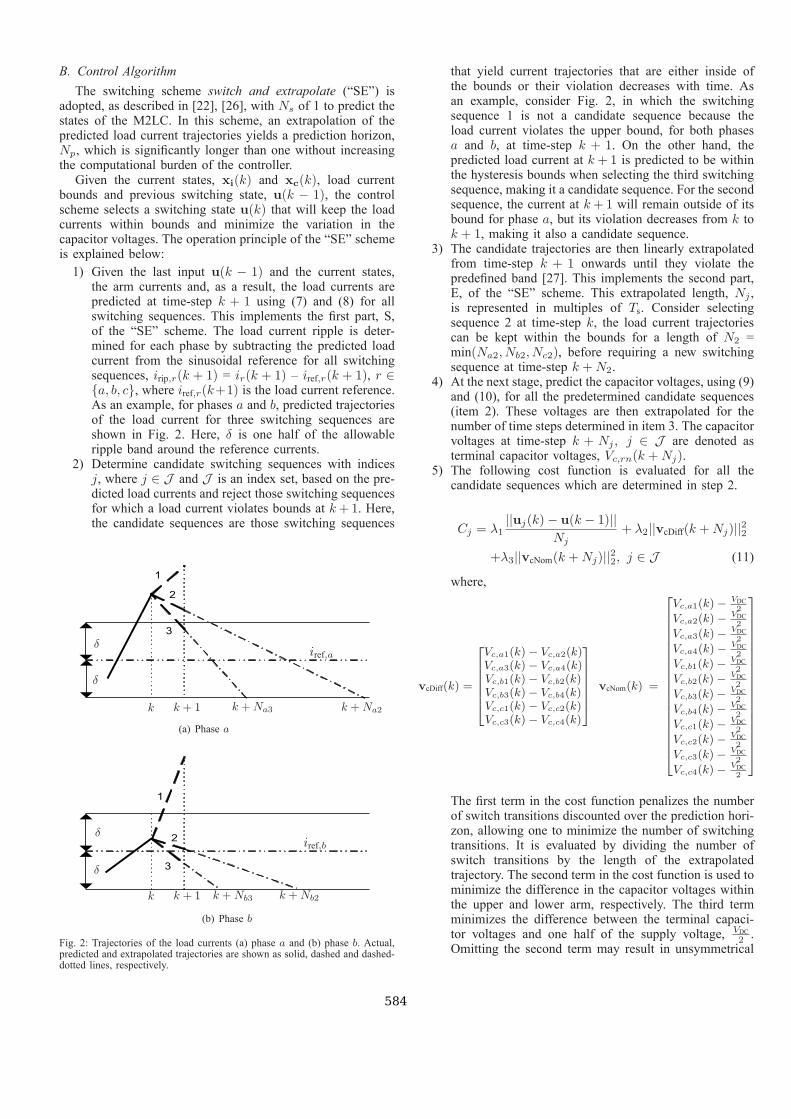
bounds and previous switching state, u(k − 1), the controlscheme selects a switching state u(k) that will keep the loadcurrents within bounds and minimize the variation in thecapacitor voltages. The operation principle of the “SE” schemeis explained below:1) Given the last input u(k − 1) and the current states,the arm currents and, as a result, the load currents arepredicted at time-step k + 1 using (7) and (8) for allswitching sequences. This implements the first part, S,of the “SE” scheme. The load current ripple is deter-mined for each phase by subtracting the predicted loadcurrent from the sinusoidal reference for all switchingsequences, irip,r(k + 1) = ir(k + 1) – iref,r(k + 1), r ∈{a, b, c}, where iref,r(k+1) is the load current reference.As an example, for phases a and b, predicted trajectoriesof the load current for three switching sequences areshown in Fig. 2. Here, δ is one half of the allowableripple band around the reference currents.

2) Determine candidate switching sequences with indicesj, where j ∈ J and J is an index set, based on the pre-dicted load currents and reject those switching sequencesfor which a load current violates bounds at k+1. Here,the candidate sequences are those switching sequences

1

2

3

δ

δiref,a

k k + 1 k +Na3 k +Na2

(a) Phase a

3

2

1

δ

δiref,b

k k + 1 k +Nb3 k +Nb2

(b) Phase b

Fig. 2: Trajectories of the load currents (a) phase a and (b) phase b. Actual,predicted and extrapolated trajectories are shown as solid, dashed and dashed-dotted lines, respectively.

that yield current trajectories that are either inside ofthe bounds or their violation decreases with time. Asan example, consider Fig. 2, in which the switchingsequence 1 is not a candidate sequence because theload current violates the upper bound, for both phasesa and b, at time-step k + 1. On the other hand, thepredicted load current at k+ 1 is predicted to be withinthe hysteresis bounds when selecting the third switchingsequence, making it a candidate sequence. For the secondsequence, the current at k+1 will remain outside of itsbound for phase a, but its violation decreases from k tok + 1, making it also a candidate sequence.

3) The candidate trajectories are then linearly extrapolatedfrom time-step k + 1 onwards until they violate thepredefined band [27]. This implements the second part,E, of the “SE” scheme. This extrapolated length, Nj ,is represented in multiples of Ts. Consider selectingsequence 2 at time-step k, the load current trajectoriescan be kept within the bounds for a length of N2 =min(Na2, Nb2, Nc2), before requiring a new switchingsequence at time-step k +N2.

4) At the next stage, predict the capacitor voltages, using (9)and (10), for all the predetermined candidate sequences(item 2). These voltages are then extrapolated for thenumber of time steps determined in item 3. The capacitorvoltages at time-step k + Nj , j ∈ J are denoted asterminal capacitor voltages, Vc,rn(k +Nj).

5) The following cost function is evaluated for all thecandidate sequences which are determined in step 2.

Cj = λ1

||uj(k)− u(k − 1)||Nj

+ λ2||vcDiff(k +Nj)||22+λ3||vcNom(k +Nj)||22, j ∈ J (11)

where,

vcDiff(k) =

⎡⎢⎢⎢⎢⎢⎣

Vc,a1(k)− Vc,a2(k)Vc,a3(k)− Vc,a4(k)Vc,b1(k)− Vc,b2(k)Vc,b3(k)− Vc,b4(k)Vc,c1(k)− Vc,c2(k)Vc,c3(k)− Vc,c4(k)

⎤⎥⎥⎥⎥⎥⎦

vcNom(k) =

⎡⎢⎢⎢⎢⎢⎢⎢⎢⎢⎢⎢⎢⎢⎢⎢⎢⎢⎢⎢⎣

Vc,a1(k)−VDC2

Vc,a2(k)−VDC2

Vc,a3(k)−VDC2

Vc,a4(k)−VDC2

Vc,b1(k)−VDC2

Vc,b2(k)−VDC2

Vc,b3(k)−VDC2

Vc,b4(k)−VDC2

Vc,c1(k)−VDC2

Vc,c2(k)−VDC2

Vc,c3(k)−VDC2

Vc,c4(k)−VDC2

⎤⎥⎥⎥⎥⎥⎥⎥⎥⎥⎥⎥⎥⎥⎥⎥⎥⎥⎥⎥⎦

The first term in the cost function penalizes the numberof switch transitions discounted over the prediction hori-zon, allowing one to minimize the number of switchingtransitions. It is evaluated by dividing the number ofswitch transitions by the length of the extrapolatedtrajectory. The second term in the cost function is used tominimize the difference in the capacitor voltages withinthe upper and lower arm, respectively. The third termminimizes the difference between the terminal capaci-tor voltages and one half of the supply voltage, VDC

2.

Omitting the second term may result in unsymmetrical

584

capacitor voltages within an arm, because the thirdterm only sets a reference for the average value of thecapacitor voltages.Here, λ1, λ2 and λ3 are the weighting coefficients andheuristic approach was followed to select their values.

6) The switching sequence with the minimum cost is se-lected and implemented at time-step k.

A receding horizon policy is implemented by repeatingthese steps at the next sampling instant. Furthermore, addi-tional control objectives can be easily included by adding themto the cost function.Total Demand Distortion (TDD) of the load current can

be controlled by adjusting the ripple δ. There is a linearrelationship between TDD and the δ band as presented in [22],where the TDD is a measure of the load current harmonicdistortion.

IV. PERFORMANCE EVALUATIONPerformance of the MPDCC scheme was investigated, using

PLECS/SIMULINK, for a 2MVA three-level M2LC and com-pared with a vector control (VC) scheme with a pulse widthmodulator. In the latter scheme, load currents in abc framewere transformed into dq quantities, followed by comparisonwith their reference values of id,ref = 1 and iq,ref = 0 and,finally, proportional-integral (PI) controllers were employedto generate voltage reference in each phase. The dq voltagereferences, were then transformed to abc domain and comparedagainst carrier waveforms in phase disposition (PD) to generatethe gating signals for the modules. The frequency of the carrierwaveform was 750 Hz and a third harmonic was injected inthe reference signals using a min-max approach that achievesthe same switching sequences as space vector modulation[28]. The capacitor voltages were balanced by using a sortingalgorithm, which was based on the polarity of the arm currents[4], [9], [17], [19]. For example, for a positive arm current thecapacitor with lowest voltage was selected first, and conversely,the capacitor with the highest voltage was prioritized for anegative arm current. The circuit parameters used for thesimulations are summarized in Table I, using VB =

√2/3Vll

= 2449.49 V, IB =√2Irat= 544.47 A and fB = 50 Hz as base

quantities for the p.u. system.

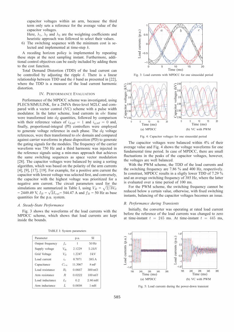
A. Steady-State PerformanceFig. 3 shows the waveforms of the load currents with the

MPDCC scheme, which shows that load currents are keptinside the bounds.

TABLE I: System parameters

Parameter p.u. SI

Output frequency fo 1 50Hz

Supply voltage Vdc 2.1229 5.2 kV

Grid Voltage Vll 1.2247 3 kV

Load current ir 0.7071 385A

Capacitance Crn 11.3067 8mF

Load resistance Rl 0.0667 300mΩ

Arm resistance R 0.0222 100mΩ

Load inductance Ll 0.2 2.86mH

Arm inductance L 0.0698 1mH

0 5 10 15 20−1

−0.5

0

0.5

1

Time (ms)

Loadcurrents(p.u.) a b c

Fig. 3: Load currents with MPDCC for one sinusoidal period

0 5 10 15 202.54

2.56

2.58

2.6

2.62

2.64

Time (ms)Capacitorvoltages(kV)

(a) MPDCC

0 5 10 15 202.54

2.56

2.58

2.6

2.62

2.64

Time (ms)

Capacitorvoltages(kV)

(b) VC with PWM

Fig. 4: Capacitor voltages for one sinusoidal period

The capacitor voltages were balanced within 4% of theiraverage value and Fig. 4 shows the voltage waveforms for onefundamental time period. In case of MPDCC, there are smallfluctuations in the peaks of the capacitor voltages, however,the voltages are well balanced.With the PWM scheme, the TDD of the load currents and

the switching frequency are 7.86 % and 400 Hz, respectively.In constrast, MPDCC results in a sligtly lower TDD of 7.29 %and an average switching frequency of 385 Hz, where the latteris evaluated over a time period of 100 ms.For the PWM scheme, the switching frequency cannot be

reduced below a certain value, otherwise, with fixed switchinginstants, balancing of the capacitor voltages becomes an issue.

B. Performance during TransientsInitially, the converter was operating at rated load current

before the reference of the load currents was changed to zeroat time-instant t = 245 ms. At time-instant t = 445 ms,

195 245 295 345 395

−1.47

−1

−0.5

0

0.5

1

1.47

Time (ms)

Loadcurrents(p.u.)

(a) MPDCC

195 245 295 345 395−1.47

−1

−0.5

0

0.5

1

1.47

Time (ms)

Loadcurrents(p.u.)

(b) VC with PWM

Fig. 5: Load currents during the power-down transient

585

395 445 495 545 595

−1.47

−1

−0.5

0

0.5

1

1.47

Time (ms)

Loadcurrents(p.u.)

(a) MPDCC

395 445 495 545 595−1.47

−1

−0.5

0

0.5

1

1.47

Time (ms)Loadcurrents(p.u.)

(b) VC with PWM

Fig. 6: Load currents during the power-up transient

195 245 295 345 3952.45

2.5

2.55

2.6

2.65

2.7

Time (ms)

Capacitorvoltages(kV)

(a) MPDCC

195 245 295 345 3952.45

2.5

2.55

2.6

2.65

2.7

Time (ms)

Capacitorvoltages(kV)

(b) VC with PWM

Fig. 7: Capacitor voltages during the power-down transient

the load current reference was changed back to 1 p.u. Theload current ripple, δ = 0.1 p.u., was not changed during thetransient operation.As shown in Fig. 5 and Fig. 6, MPDCC achieves a very fast

current response both at power-down and power-up. It takesless than 3 ms to deliver the rated load currents. On the otherhand, the PWM scheme provides a slow response. Fig. 6 showsthat the load currents overshoot at power-up before settling attheir nominal values. With PWM scheme, the current responsemight not be further improved because increasing PI gainsbeyond certain values will result in an unstable oscillations inthe load currents.With the MPDCC scheme, the capacitor voltages, as shown

in Fig. 7 and Fig. 8, are well balanced both at power-down and power-up. After power-up, the capacitor voltagessettle within 4% of the average voltage value in less thanthree sinusoidal periods. Whereas, with the PWM scheme,

395 445 495 545 5952.45

2.5

2.55

2.6

2.65

2.7

Time (ms)

Capacitorvoltages(kV)

(a) MPDCC

395 445 495 545 5952.45

2.5

2.55

2.6

2.65

2.7

Time (ms)

Capacitorvoltages(kV)

(b) VC with PWM

Fig. 8: Capacitor voltages during the during the power-up transient

the capacitor voltages exhibit large oscillations both at power-down and power-up.During the transients, the converter rapidly changes the

arm currents to meet the load current requirements. Duringthis period, the arm inductors and capacitors exchange energy,resulting in an overshoot of the capacitor voltages at power-down and power-up. This overshoot in the voltage can befurther minimized by controlling the rate of change of the loadcurrent’s reference trajectory or with an appropriate design ofthe arm inductor.

V. CONCLUSIONSMPDCC with a long prediction horizon for the control of

the M2LC has been presented in this paper. It has been shownthat the MPDCC requires a single control loop, without amodulator, to control the load currents within tight boundsaround their sinusoidal references, balance the capacitor volt-ages and minimize the switching frequency in comparison toexisting hierarchical control schemes. Simulated results havebeen presented to validate the viability of the proposed controltechnique. Furthermore, it has been shown that the MPDCCscheme achieves very fast current responses during transients,such as power-up and power-down. The capacitor voltageshave been kept close to their reference values both duringtransients and steady-state operating conditions. In addition,comparison with a vector control PWM scheme has shownthat improvements in performance with the MPDCC.

APPENDIX ATHE DISCRETE-TIME MATRICES OF THE MODELS

Ai = eT−1

FiTs (12)

Bi = Fi−1T(Ai − I1)T

−1Gi (13)

T =

⎡⎢⎢⎢⎢⎢⎢⎢⎢⎣

L L 0 0 0 0 00 0 L L 0 0 0−L −L −L −L 2L 0 0−Ll L+ Ll Ll −L− Ll 0 0 02Ll −2L− 2Ll Ll −L− Ll L 0 00 0 0 0 0 1 00 0 0 0 0 0 1

⎤⎥⎥⎥⎥⎥⎥⎥⎥⎦

Fi =

⎡⎢⎢⎢⎢⎢⎢⎢⎢⎣

−R −R 0 0 2R

30 0

0 0 −R −R2R

30 0

R R R R−4R

30 0

Rl −R−Rl −Rl R+Rl 0 3

2

−√3

2

−2Rl 2R+ 2Rl −Rl R+Rl −R−3

2

−√3

2

0 0 0 0 0 0 −ω

0 0 0 0 0 ω 0

⎤⎥⎥⎥⎥⎥⎥⎥⎥⎦

Here, I1 represents an identity matrix of a relevant order.

Ac = eFcTs (14)

Bc = Fc−1(Ac − I2)Gc (15)

586

Gi =

⎡⎢⎢⎢⎢⎢⎢⎢⎢⎣

−

2

3Vc,a1 −

2

3Vc,a2 −

2

3Vc,a3 −

2

3Vc,a4

Vc,b1

3

Vc,b2

3

Vc,b3

3

Vc,b4

3

Vc,c1

3

Vc,c2

3

Vc,c3

3

Vc,c4

3Vc,a1

3

Vc,a2

3

Vc,a3

3

Vc,a4

3−

2

3Vc,b1 −

2

3Vc,b2 −

2

3Vc,b3 −

2

3Vc,b4

Vc,c1

3

Vc,c2

3

Vc,c3

3

Vc,c4

3Vc,a1

3

Vc,a2

3

Vc,a3

3

Vc,a4

3

Vc,b1

3

Vc,b2

3

Vc,b3

3

Vc,b4

3−

2

3Vc,c1 −

2

3Vc,c2 −

2

3Vc,c3 −

2

3Vc,c4

0 0 −Vc,a3 −Vc,a4 0 0 Vc,b3 Vc,b4 0 0 0 00 0 Vc,a3 Vc,a4 0 0 0 0 0 0 −Vc,c3 −Vc,c4

0 0 0 0 0 0 0 0 0 0 0 00 0 0 0 0 0 0 0 0 0 0 0

⎤⎥⎥⎥⎥⎥⎥⎥⎥⎦

Fc = − 1

CrnRcapI2 (16)

Cc = I2 (17)

Ci =

⎡⎣

1 −1 0 0 00 0 1 −1 0−1 1 −1 1 0

⎤⎦ (18)

Gc =1

Crn

diag(iaP, iaP, iaN, iaN, ibP, ibP, ibN, ibN, icP, icP,

icN, icN) (19)

Here, I2 represents an identity matrix of a relevant orderand diag(...) is a square diagonal matrix with entries inside thebrackets at its main diagonal [ � ].

ACKNOWLEDGMENTThe authors thank James Scoltock of the University of

Auckland for his advice. This work was supported by TheUniversity of Auckland Doctoral Scholarship.

REFERENCES[1] S. Allebrod, R. Hamerski, and R. Marquardt. New transformerless,

scalable modular multilevel converters for HVDC-transmission. In Proc.IEEE Power Electronics Specialists Conf. PESC, pages 174–179, 2008.

[2] U. N. Gnanarathna, S. K. Chaudhary, A. M. Gole, and R. Teodorescu.Modular multi-level converter based HVDC system for grid connectionof offshore wind power plant. In 9th IET International Conference onAC and DC Power Transmission, ACDC., pages 1–5, 2010.

[3] B. Gemmell, J. Dorn, D. Retzmann, and D. Soerangr. Prospects ofmultilevel VSC technologies for power transmission. In Proc. IEEE/PEST&D Transmission and Distribution Conf. and Exposition, pages 1–16,2008.

[4] M. Saeedifard and R. Iravani. Dynamic performance of a modularmultilevel back-to-back HVDC system. IEEE Transactions on PowerDelivery,, 25(4):2903–2912, 2010.

[5] M. Hagiwara, K. Nishimura, and H. Akagi. A medium-voltage motordrive with a modular multilevel pwm inverter. IEEE Transactions onPower Electronics,, 25(7):1786–1799, 2010.

[6] M. Hiller, D. Krug, R. Sommer, and S. Rohner. A new highly modularmedium voltage converter topology for industrial drive applications. InProc. 13th European Conf. Power Electronics and Applications EPE ’09,pages 1–10, 2009.

[7] A. Antonopoulos, K. Ilves, L. Angquist, and H.-P. Nee. On in-teraction between internal converter dynamics and current control ofhigh-performance high-power ac motor drives with modular multilevelconverters. In Proc. IEEE Energy Conversion Congress and Exposition(ECCE), pages 4293–4298, 2010.

[8] A. J. Korn, M. Winkelnkemper, and P. Steimer. Low output frequencyoperation of the modular multi-level converter. In Proc. IEEE EnergyConversion Congress and Exposition (ECCE), pages 3993–3997, 2010.

[9] M. Glinka and R. Marquardt. A new AC/AC-multilevel converter familyapplied to a single-phase converter. In The Fifth International Conferenceon Power Electronics and Drive Systems, PEDS, pages 16–23, 2003.

[10] M. Glinka and R. Marquardt. A new AC/AC multilevel converter family.IEEE Transactions on Industrial Electronics, 52(3):662–669, Jun. 2005.

[11] M. Hagiwara, R. Maeda, and H. Akagi. Negative-sequence reactive-power control by the modular multilevel cascade converter based ondouble-star chopper-cells (MMCC-DSCC). In Proc. IEEE EnergyConversion Congress and Exposition (ECCE), pages 3949–3954, 2010.

[12] H. P. Mohammadi and M. T. Bina. A transformerless medium-voltageSTATCOM topology based on extended modular multilevel converters.IEEE Transactions on Power Electronics,, 26(5):1534–1545, 2011.

[13] A. Lesnicar and R. Marquardt. An innovative modular multilevelconverter topology suitable for a wide power range. In Proc. IEEEPower Tech. Conf., Bologna, Italy, Jun. 2003.

[14] M. Glinka. Prototype of multiphase modular-multilevel-converter with2 MW power rating and 17-level-output-voltage. In Proc. IEEE 35thAnnual Power Electronics Specialists Conf. PESC 04, pages 2572–2576,2004.

[15] G. P. Adam, K. H. Ahmed, S. J. Finney, and B. W. Williams. Modularmultilevel converter for medium-voltage applications. In Proc. IEEE Int.Electric Machines & Drives Conf. (IEMDC), pages 1013–1018, 2011.

[16] A. Antonopoulos, L. Angquist, and H.-P. Nee. On dynamics and voltagecontrol of the modular multilevel converter. In Proc. 13th European Conf.Power Electronics and Applications EPE ’09, pages 1–10, 2009.

[17] S. Rohner, S. Bernet, M. Hiller, and R. Sommer. Pulse width modulationscheme for the modular multilevel converter. In Proc. 13th EuropeanConf. Power Electronics and Applications EPE ’09, pages 1–10, 2009.

[18] M. Hagiwara and H. Akagi. Control and experiment of pulsewidth-modulated modular multilevel converters. IEEE Transactions on PowerElectronics, 24(7):1737–1746, Jul. 2009.

[19] G. P. Adam, O. Anaya-Lara, G. M. Burt, D. Telford, B. W. Williams, andJ. R. McDonald. Modular multilevel inverter: pulse width modulationand capacitor balancing technique. Power Electronics, IET, 3(5):702–715, 2010.

[20] M. A. Perez, J. Rodriguez, E. J. Fuentes, and F. Kammerer. Predictivecontrol of AC–AC modular multilevel converters. IEEE Trans. Ind.Electron., 59(7):2832–2839, 2012.

[21] S. P. Engel and R. W. De Doncker. Control of the modular multi-levelconverter for minimized cell capacitance. In Proc. 2011-14th EuropeanConf. Power Electronics and Applications (EPE 2011), pages 1–10,2011.

[22] T. Geyer. Model predictive direct current control for multi-level convert-ers. In Proc. IEEE Energy Conversion Congress and Exposition (ECCE),pages 4305–4312, 2010.

[23] G. S. Konstantinou, M. Ciobotaru, and V. G. Agelidis. Analysis ofmulti-carrier PWM methods for back-to-back HVDC systems based onmodular multilevel converters. In Proc. IECON 2011 - 37th AnnualConf. IEEE Industrial Electronics Society, pages 4391–4396, 2011.

[24] J. M. Maciejowski. Predictive Control. Prentice Hall, 2002.[25] J. B. Rawlings and D. Q. Mayne. Model predictive control: Theory and

design. Nob Hill Publ., 2009.[26] T. Geyer. Generalized model predictive direct torque control: Long

prediction horizons and minimization of switching losses. In Proc. IEEEConf. Decision Control, pages 6799–6804, Shanghai, China, Dec. 2009.

[27] Y. Zeinaly, T. Geyer, and B. Egardt. Trajectory extension methods formodel predictive direct torque control. In Proc. App. Power Electron.Conf. and Expo., Fort Worth, TX, USA, Mar. 2011.

[28] B. P. McGrath, D. G. Holmes, and T. Lipo. Optimized space vectorswitching sequences for multilevel inverters. IEEE Trans. Power Elec-tron., 18(6):1293–1301, Nov. 2003.

587

Powered by TCPDF (www.tcpdf.org)