Download - Matrix representations of octonions and their applications

arX

iv:m

ath/

0003

166v

2 [

mat

h.R

A]

1 A

pr 2

000

MATRIX REPRESENTATIONS OF OCTONIONS AND

THEIR APPLICATIONS

Yongge Tian

Department of Mathematics and Statistics

Queen’s University

Kingston, Ontario, Canada K7L 3N6

e-mail:[email protected]

Abstract

As is well-known, the real quaternion division algebra H is algebraically isomorphic to a 4-by-4

real matrix algebra. But the real division octonion algebra O can not be algebraically isomorphic

to any matrix algebras over the real number field R, because O is a non-associative algebra over R.

However since O is an extension of H by the Cayley-Dickson process and is also finite-dimensional,

some pseudo real matrix representations of octonions can still be introduced through real matrix

representations of quaternions. In this paper we give a complete investigation to real matrix repre-

sentations of octonions, and consider their various applications to octonions as well as matrices of

octonions.

AMS Mathematics Subject Classification: 15A33; 15A06; 15A24; 17A35

Key Words: quaternions, octonions, matrix representations, linear equations, similarity, eigenvalues,

Cayley-Hamilton theorem

1. Introduction

Let O be the octonion algebra over the real number field R. Then it is well known by the Cayley-Dickson

process that any a ∈ O can be written as

a = a′ + a′′e, (1.1)

where a′, a′′ ∈ H = { a = a0 + a1i + a2j + a3k | i2 = j2 = k2 = −1, ijk = −1, a0—a3 ∈ R }, the real

quaternion division algebra. The addition and multiplication for any a = a′ + a′′e, b = b′ + b′′e ∈ O are

defined by

a + b = ( a′ + a′′e ) + ( b′ + b′′e) = ( a′ + b′ ) + ( a′′ + b′′ )e, (1.2)

and

ab = ( a′ + a′′e)(b′ + b′′e) = (a′b′ − b′′a′′) + (b′′a′ + a′′b′ )e, (1.3)

where b′, b′′ denote the conjugates of the quaternions b′ and b′′. In that case, O is an eight-dimensional

non-associative but alternative division algebra over its center field R, and the canonical basis of O is

1, e1 = i, e2 = j, e3 = k, e4 = e, e5 = ie, e6 = je, e7 = ke. (1.4)

1

http://arXiv.org/abs/math/0003166v2

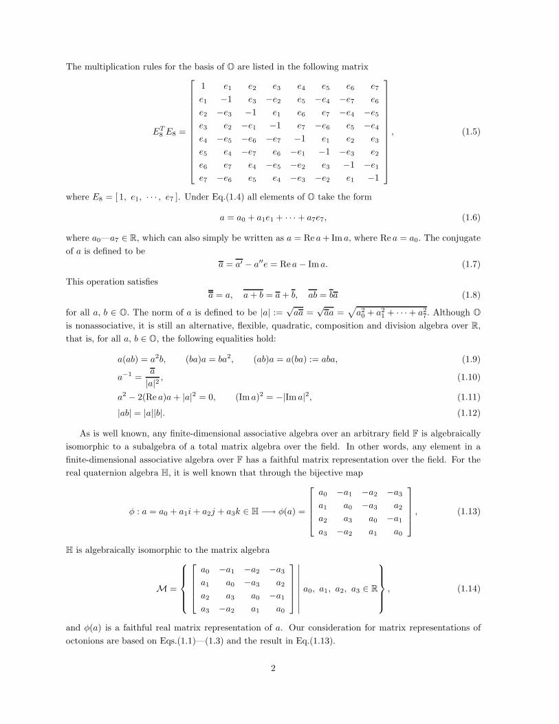
The multiplication rules for the basis of O are listed in the following matrix

ET8 E8 =

1 e1 e2 e3 e4 e5 e6 e7

e1 −1 e3 −e2 e5 −e4 −e7 e6

e2 −e3 −1 e1 e6 e7 −e4 −e5

e3 e2 −e1 −1 e7 −e6 e5 −e4

e4 −e5 −e6 −e7 −1 e1 e2 e3

e5 e4 −e7 e6 −e1 −1 −e3 e2

e6 e7 e4 −e5 −e2 e3 −1 −e1

e7 −e6 e5 e4 −e3 −e2 e1 −1

, (1.5)

where E8 = [ 1, e1, · · · , e7 ]. Under Eq.(1.4) all elements of O take the form

a = a0 + a1e1 + · · · + a7e7, (1.6)

where a0—a7 ∈ R, which can also simply be written as a = Re a + Im a, where Re a = a0. The conjugate

of a is defined to be

a = a′ − a′′e = Rea − Im a. (1.7)

This operation satisfies

a = a, a + b = a + b, ab = ba (1.8)

for all a, b ∈ O. The norm of a is defined to be |a| :=√

aa =√

aa =√

a20 + a2

1 + · · · + a27. Although O

is nonassociative, it is still an alternative, flexible, quadratic, composition and division algebra over R,

that is, for all a, b ∈ O, the following equalities hold:

a(ab) = a2b, (ba)a = ba2, (ab)a = a(ba) := aba, (1.9)

a−1 =a

|a|2 , (1.10)

a2 − 2(Re a)a + |a|2 = 0, (Im a)2 = −|Im a|2, (1.11)

|ab| = |a||b|. (1.12)

As is well known, any finite-dimensional associative algebra over an arbitrary field F is algebraically

isomorphic to a subalgebra of a total matrix algebra over the field. In other words, any element in a

finite-dimensional associative algebra over F has a faithful matrix representation over the field. For the

real quaternion algebra H, it is well known that through the bijective map

φ : a = a0 + a1i + a2j + a3k ∈ H −→ φ(a) =

a0 −a1 −a2 −a3

a1 a0 −a3 a2

a2 a3 a0 −a1

a3 −a2 a1 a0

, (1.13)

H is algebraically isomorphic to the matrix algebra

M =

a0 −a1 −a2 −a3

a1 a0 −a3 a2

a2 a3 a0 −a1

a3 −a2 a1 a0

∣∣∣∣∣∣∣∣∣

a0, a1, a2, a3 ∈ R

, (1.14)

and φ(a) is a faithful real matrix representation of a. Our consideration for matrix representations of

octonions are based on Eqs.(1.1)—(1.3) and the result in Eq.(1.13).

2

We next present some basic results related to matrix representations of quaternions, which will be

serve as a tool for our examination in the sequel.

Lemma 1.1[13]. Let a = a0 + a1i + a2j + a3k ∈ H be given, where a0—a3 ∈ R. Then the diagonal

matrix diag( a, a, a, a ) satisfies the following unitary similarity factorization equality

Q

a

a

a

a

Q∗ =

a0 −a1 −a2 −a3

a1 a0 −a3 a2

a2 a3 a0 −a1

a3 −a2 a1 a0

∈ R

4×4, (1.15)

where the matrix Q has the following independent expression

Q = Q∗ =1

2

1 i j k

−i 1 k −j

−j −k 1 i

−k j −i 1

, (1.16)

which is a unitary matrix over H.

Lemma 1.2[13]. Let a, b ∈ H, and λ ∈ R. Then

(a) a = b ⇐⇒ φ(a) = φ(b).

(b) φ(a + b) = φ(a) + φ(b), φ(ab) = φ(a)φ(b), φ(λa) = λφ(a), φ(1) = I4.

(c) a = 14E4φ(a)E∗

4 , where E4 := [ 1, i, j, k ] and E∗4 := [ 1, −i, −j, −k ]T .

(d) φ(a) = φT (a).

(e) φ(a−1) = φ−1(a), if a 6= 0.

(f) det [φ(a)] = |a|4.

We can also introduce from Eq.(1.13) another real matrix representation of a as follows

τ(a) := KφT (a)K =

a0 −a1 −a2 −a3

a1 a0 a3 −a2

a2 −a3 a0 a1

a3 a2 −a1 a0

, (1.17)

where K = diag( 1, −1, −1, −1 ). Some basic operation properties on τ(a) are

τ(a + b) = τ(a) + τ(b), τ(ab) = τ(b)τ(a), τ(a) = τT (a), (1.18)

det [φ(a)] = |a|4, φ(a−1) = φ−1(a) if a 6= 0. (1.19)

Combining the two real matrix representations of quaternions with their real vector representations,

we have the following important result.

Lemma 1.3. Let x = x0 + x1i + x2j + x3k ∈ H, and denote −→x = [ x0, x1, x2, x3 ]T , called the vector

representation of x. Then for all a, b, x ∈ H, we have

−→ax = φ(a)−→x ,−→xb = τ(b)−→x ,

−→axb = φ(a)τ(b)−→x = τ(b)φ(a)−→x , (1.20)

and the equality

φ(a)τ(b) = τ(b)φ(a) (1.21)

3

always holds.

Proof. Observe that

−→x = φ(x)αT4 , −→x = τ(x)αT

4 , α4 = [ 1, 0, 0, 0 ].

We find by Lemma 1.1 and Eq.(1.2) that

−→ax = φ(ax)αT4 = φ(a)φ(x)αT

4 = φ(a)−→x ,−→xb = τ(xb)αT

4 = τ(b)τ(x)αT4 = τ(b)−→x ,

and−→axb =

−−−→a(xb) = φ(a)

−−→(xb) = φ(a)τ(b)−→x ,

−→axb =

−−−→(ax)b = τ(b)

−−→(ax) = τ(b)φ(a)−→x .

These four equalities are exactly the results in Eqs.(1.20) and (1.21). 2

Lemma 1.4[12][17]. Let a, b, x ∈ O be given. Then

(a) Re (ab) = Re (ba), Re ((ax)b) = Re (a(xb)).

(b) (aba)x = a(b(ax)), x(aba) = ((xa)b)a.

(c) (ab)(xa) = a(bx)a, (bx)(ab) = b(xa)b.

(d) (a, b, x) = −(a, x, b) = (x, a, b), where (a, b, x) = (ab)x − a(bx).

2. The real matrix representations of octonions

Based on the results on the real matrix representation of quaternions, we now can introduce real matrix

representation of octonions.

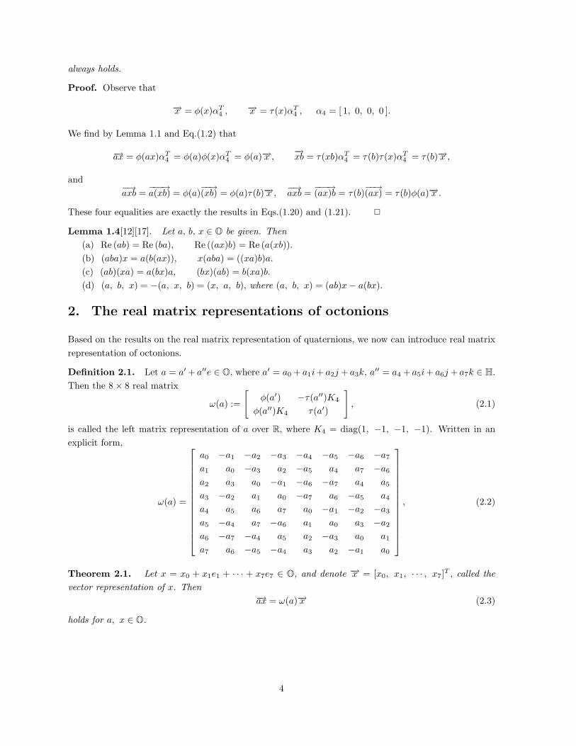
Definition 2.1. Let a = a′ + a′′e ∈ O, where a′ = a0 + a1i + a2j + a3k, a′′ = a4 + a5i + a6j + a7k ∈ H.

Then the 8 × 8 real matrix

ω(a) :=

[φ(a′) −τ(a′′)K4

φ(a′′)K4 τ(a′)

], (2.1)

is called the left matrix representation of a over R, where K4 = diag(1, −1, −1, −1). Written in an

explicit form,

ω(a) =

a0 −a1 −a2 −a3 −a4 −a5 −a6 −a7

a1 a0 −a3 a2 −a5 a4 a7 −a6

a2 a3 a0 −a1 −a6 −a7 a4 a5

a3 −a2 a1 a0 −a7 a6 −a5 a4

a4 a5 a6 a7 a0 −a1 −a2 −a3

a5 −a4 a7 −a6 a1 a0 a3 −a2

a6 −a7 −a4 a5 a2 −a3 a0 a1

a7 a6 −a5 −a4 a3 a2 −a1 a0

, (2.2)

Theorem 2.1. Let x = x0 + x1e1 + · · · + x7e7 ∈ O, and denote −→x = [x0, x1, · · · , x7]T , called the

vector representation of x. Then−→ax = ω(a)−→x (2.3)

holds for a, x ∈ O.

4

Proof. Write a, x ∈ O as a = a′ + a′′e, x = x′ + x′′e, where a′, a′′, x′, x′′ ∈ H. We know by Eq.(1.3)

that ax = (a′x′ − x′′a′′) + (x′′a′ + a′′x′)e. Thus it follows by Eq.(1.20) that

−→ax =

[ −−−−−−−−→a′x′ − x′′a′′

−−−−−−−−→x′′a′ + a′′x′

]=

[ −−→a′x′ −

−−−→x′′a′′

−−→x′′a′ +

−−→a′′x′

]

=

[φ(a′)

−→x′ − τ(a′′)K4

−→x′′

τ(a′)−→x′′ + φ(a′′)K4

−→x′

]

=

[φ(a′) −τ(a′′)K4

φ(a′′)K4 τ(a′)

][ −→x′

−→x′′

],

as required for Eq.(2.3). 2

Theorem 2.2. Let a ∈ O be given. Then

aE8 = E8ω(a), and E∗8a = ω(a)E∗

8 , (2.4)

where E8 := [ 1, e1, · · · , e7 ], and E∗8 := [ 1, −e1, · · · , −e7 ]T .

Proof. Follows from a direct verification. 2

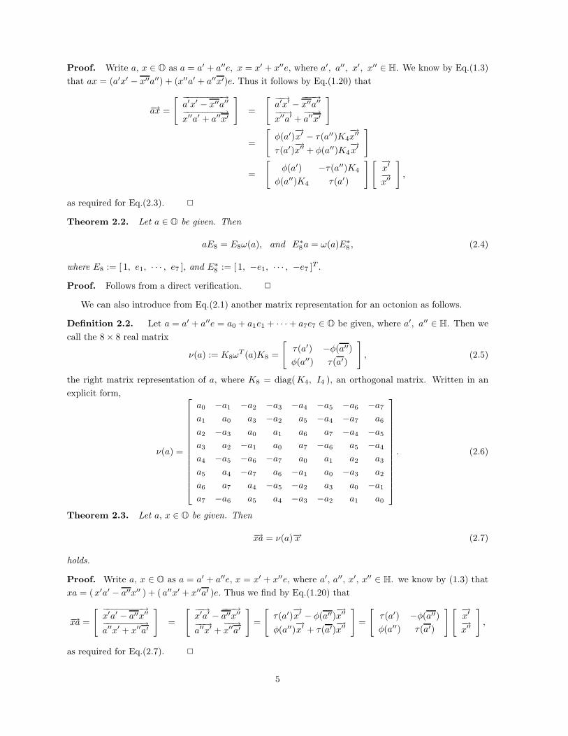
We can also introduce from Eq.(2.1) another matrix representation for an octonion as follows.

Definition 2.2. Let a = a′ + a′′e = a0 + a1e1 + · · · + a7e7 ∈ O be given, where a′, a′′ ∈ H. Then we

call the 8 × 8 real matrix

ν(a) := K8ωT (a)K8 =

[τ(a′) −φ(a′′)

φ(a′′) τ(a′)

], (2.5)

the right matrix representation of a, where K8 = diag(K4, I4 ), an orthogonal matrix. Written in an

explicit form,

ν(a) =

a0 −a1 −a2 −a3 −a4 −a5 −a6 −a7

a1 a0 a3 −a2 a5 −a4 −a7 a6

a2 −a3 a0 a1 a6 a7 −a4 −a5

a3 a2 −a1 a0 a7 −a6 a5 −a4

a4 −a5 −a6 −a7 a0 a1 a2 a3

a5 a4 −a7 a6 −a1 a0 −a3 a2

a6 a7 a4 −a5 −a2 a3 a0 −a1

a7 −a6 a5 a4 −a3 −a2 a1 a0

. (2.6)

Theorem 2.3. Let a, x ∈ O be given. Then

−→xa = ν(a)−→x (2.7)

holds.

Proof. Write a, x ∈ O as a = a′ + a′′e, x = x′ + x′′e, where a′, a′′, x′, x′′ ∈ H. we know by (1.3) that

xa = (x′a′ − a′′x′′ ) + ( a′′x′ + x′′a′ )e. Thus we find by Eq.(1.20) that

−→xa =

[ −−−−−−−−→x′a′ − a′′x′′

−−−−−−−−→a′′x′ + x′′a′

]=

[ −−→x′a′ −

−−−→a′′x′′

−−→a′′x′ +

−−→x′′a′

]=

[τ(a′)

−→x′ − φ(a′′)

−→x′′

φ(a′′)−→x′ + τ(a′)

−→x′′

]=

[τ(a′) −φ(a′′)

φ(a′′) τ(a′)

][ −→x′

−→x′′

],


5


aF8 = F8νT (a), and F ∗

8 a = νT (a)F ∗8 , (2.8)

where F8 := [ 1, −e1, · · · , −e7 ] and F ∗8 := [ 1, e1, · · · , e7 ]T .


Observe from Eqs.(2.1) and (2.5) that the two real matrix representations of an octonion a = a′ +a′′e

are in fact constructed by the real matrix representations of two quaternions a′ and a′′. Hence the

operation properties for the two matrix representations of octonions can easily be established through

the results in Lemmas 1.2 and 1.3.

Theorem 2.5. Let a, b ∈ O, λ ∈ R be given. Then

(a) a = b ⇐⇒ ω(a) = ω(b).

(b) ω(a + b) = ω(a) + ω(b), ω(λa) = λω(a), ω(1) = I8.

(c) ω(a) = ωT (a).


Theorem 2.6. Let a, b ∈ O, λ ∈ R be given. Then

(a) a = b ⇐⇒ ν(a) = ν(b).

(b) ν(a + b) = ν(a) + ν(b), ν(λa) = λν(a), ν(1) = I8.

(c) ν(a) = νT (a).



a =1

8E8ω(a)E∗

8 , and a =1

8F8ν

T (a)F ∗8 , (2.9)

where E8, E∗8 , F8 and F ∗

8 are as in Eqs.(2.4) and (2.8).

Proof. Note that ω(a) and ν(a) are real matrices. Thus we get from Eqs.(2.4) and (2.8) that

E8(E∗8a) = E8[ω(a)E∗

8 ] = E8ω(a)E∗8 , and F (F ∗

8 a) = F8[νT (a)F ∗

8 ] = F8νT (a)F ∗

8 .

On the other hand, note that O is alternative. It follows that

E8(E∗8a) = a − e1(e1a) − · · · − e7(e7a) = a − e2

1a − · · · − e27a = 8a,

and

F8(F∗8 a) = a − e1(e1a) − · · · − e7(e7a) = a − e2

1a − · · · − e27a = 8a.

Thus we have Eq.(2.9). 2


det [ω(a)] = det [ν(a)] = |a|8. (2.10)

Proof. Write a = a′ + a′′e. Then we easily find by Eqs.(1.21) and (2.5) that

det [ω(a)] = det [ν(a)] =

∣∣∣∣∣τ(a′) −φ(a′′)

φ(a′′) τ(a′)

∣∣∣∣∣ = det [ τ(a′)τ(a′) + φ(a′′)φ(a′′) ]

= det [ τ(a′a′) + φ(a′′a′′) ]

= det [ |a′|2I4 + |a′′|2I4 ]

= ( |a′|2 + |a′′|2 )4 = |a|8,

6


Theorem 2.9. Let a ∈ O be given. Then the two matrix representations of a satisfy the following three

identities

ω(a2) = ω2(a), ν(a2) = ν2(a), ω(a)ν(a) = ν(a)ω(a). (2.11)

Proof. Applying Eqs.(2.3) and (2.7) to the both sides of the three identities in Eq.(1.9) leads to

ω2(a)−→b = ω(a2)

−→b , ν2(a)

−→b = ν(a2)

−→b , ω(a)ν(a)

−→b = ν(a)ω(a)

−→b .

Note that−→b is an arbitrary 8 × 1 real vector when b runs over O. Thus Eq.(2.11) follows. 2

Theorem 2.10. Let a ∈ O be given with a 6= 0. Then

ω(a−1) = ω−1(a), and ν(a−1) = ν−1(a). (2.12)

Proof. Note from Eqs.(1.10) and (1.11) that

a−1 =a

|a|2 =1

|a|2 [ 2(Rea) − a ]

and

a2 − 2Re a + |a|2 = 0.

Applying Theorems 2.5 and 2.6, as well as the first two equalities in Eq.(2.11) to the both sides of the

above two equalities, we obtain

ω(a−1) =1

|a|2 [ 2(Rea)I8 − ω(a) ], ν(a−1) =1

|a|2 [ 2(Re a)I8 − ν(a) ]

and

ω2(a) − 2(Rea)ω(a) + |a|2I8 = 0, ν2(a) − 2(Rea)ν(a) + |a|2I8 = 0.

Contrasting them yields Eq.(2.12). 2

Because O is non-associative, the operation properties ω(ab) = ω(a)ω(b) and ν(ab) = ν(b)ν(a) do

not hold in general, otherwise O will be algebraically isomorphic to or algebraically anti-isomorphic to

an associative matrix algebra over R, this is impossible. Nevertheless, some other kinds of identities on

the two real matrix representations of octonions can still be established from the identities in Lemma

1.4(a)—(d).

Theorem 2.11. Let a, b ∈ O be given. Then their matrix representations satisfy the following two

identities

ω(aba) = ω(a)ω(b)ω(a), and ν(aba) = ν(a)ν(b)ν(a). (2.13)

Proof. Follows from applying Eqs.(2.3) and (2.7) to the Moufang identities in Lemma 1.4(b) . 2

Theorem 2.12. Let a, b ∈ O be given. Then their matrix representations satisfy the following identities

ω(ab) + ω(ba) = ω(a)ω(b) + ω(b)ω(a), (2.14)

ν(ab) + ν(ba) = ν(a)ν(b) + ν(b)ν(a), (2.15)

ω(ab) + ν(ab) = ω(a)ω(b) + ν(b)ν(a), (2.16)

ω(a)ν(b) + ω(b)ν(a) = ν(a)ω(b) + ν(b)ω(a), (2.17)

ω(ab) = ω(a)ω(b) + ω(a)ν(b) − ν(b)ω(a), (2.18)

ν(ab) = ν(b)ν(a) + ω(b)ν(a) − ν(a)ω(b). (2.19)

7

Proof. The identities in Lemma 1.4(d) can clearly be written as the following six identities

(ab)x − a(bx) = −(ba)x + b(ax), (xa)b − x(ab) = −(xb)a + x(ba),

(ab)x − a(bx) = −(bx)a + b(xa), (ab)x − a(bx) = −(xa)b + x(ab),

(ab)x − a(bx) = −(ax)b + a(xb), (xa)b − x(ab) = −(ax)b + a(xb).

Applying Eqs.(2.3) and (2.7) to the both sides of the above identities, we obtain

[ ω(ab) − ω(a)ω(b) ]−→x = [−ω(ba) + ω(b)ω(a) ]−→x ,

[ ν(b)ν(a) − ν(ab) ]−→x = [−ν(a)ν(b) + ν(ba) ]−→x ,

[ ν(b)ω(a) − ω(a)ν(b) ]−→x = [−ν(a)ω(b) + ω(b)ν(a) ]−→x ,

[ ω(ab) − ω(a)ω(b) ]−→x = [−ν(b)ν(a) + ν(ab) ]−→x ,

[ ω(ab) − ω(a)ω(b) ]−→x = [−ν(b)ω(a) + ω(a)ν(b) ]−→x ,

[ ν(b)ν(a) − ν(ab) ]−→x = [−ν(b)ω(a) + ω(a)ν(b) ]−→x .

Notice that −→x is an arbitrary real 8 × 1 real matrix when x runs over O. Therefore Eqs.(2.14)—(2.19)

follow. 2

Theorem 2.13. Let a, b ∈ O be given with a 6= 0, b 6= 0. Then their matrix representations satisfy the

following two identities

ω(ab) = ν(a)[ ω(a)ω(b) ]ν−1(a), and ν(ab) = ω(b)[ ν(b)ν(a) ]ω−1(b). (2.20)

which imply that

ω(ab) ∼ ω(a)ω(b), and ν(ab) ∼ ν(b)ν(a). (2.21)

Proof. Applying Eqs.(2.3) and (2.7) to the both sides of the two identities in Lemma 1.4(c), we obtain

ω(ab)ν(a)−→x = ν(a)ω(a)ω(b)−→x , and ν(ab)ω(b)−→x = ω(b)ν(b)ν(a)−→x ,

which are obviously equvalent to Eq.(2.20). 2

Note from Eqs.(2.3) and (2.7) that any linear equation of the form ax−xb = c over O can equivqlently

be written as [ ω(a) − ν(b) ]−→x = −→a , which is a linear equation over R. Thus it is necessary to consider

the operation properties of the matrix ω(a) − ν(b), especially the determinant of ω(a) − ν(b) for any

a, b ∈ O. Here we only list the expression of the determinant of ω(a) − ν(b). Its proof is quite tedious

and is, therefore, omitted here.

Theorem 2.14. Let a, b ∈ O be given and define δ(a, b) := ω(a) − ν(b). Then

det [δ(a, b)] = |a − b|4[ s2 + ( |Im a| − |Im b| )2 ][ s2 + ( |Im a| + |Im b| )2 ] (2.22)

det [δ(a, b)] = ( s2 + |Im a + Im b|2 )2[s4 + 2s2(|Im a|2 + |Im b|2) + ( |Im a|2 − |Im b|2 )2], (2.23)

where s = Re a − Re b. The characteristic polynomial of δ(a, b) is

| λI8 − δ(a, b) |= [ (λ − s )2 + |Im a + Im b|2]2[ (λ − s )2 + (|Im a| − |Im b| )2 ][ (λ − s )2 + ( |Im a| + |Im b| )2 ]. (2.24)

8

In particular, if Re a = Re b and |Im a| = |Im b|, but a 6= b, then

rank δ(a, b) = 6. (2.25)

Theorem 2.15. Let a, b ∈ O be given with a 6= 0 and b 6= 0. Then δ(a, b) = ω(a) − ν(b) is a real

normal matrix over R, that is, δ(a, b)δT (a, b) = δT (a, b)δ(a, b).

Proof. Follows from

δ(a, b) + δT (a, b) = ω(a) − ν(b) + ωT (a) − νT (b)

= ω(a) − ν(b) + ω(a) − ν(b)

= ω(a + a) − ν(b + b) = 2(Re a − Re b)I8. 2

Theorem 2.16. Let a ∈ O be given with a /∈ R. Then

δ3(a, a) = −4|Ima|2δ(a, a), (2.26)

and δ(a, a) has a generalized inverse as follows

δ−(a, a) = − 1

4|Im a|2 δ(a, a). (2.27)

Proof. Observe that δ(a, a) = ω(a) − ν(a) = ω(Im a) − ν(Im a) and (Im a)2 = −|Im a|2. Thus we

find that

δ2(a, a) = [ ω(Im a) − ν(Im a) ]2

= [ ω2(Im a) − 2ω(Im a)ν(Im a) + ν2(Im a) ]

= [ ω((Im a)2) − 2ω(Ima)ν(Im a) + ν((Im a)2) ]

= −2[ |Ima|2I8 + ω(Im a)ν(Im a) ],

and

δ3(a, a) = −2[ |Ima|2I8 + ω(Im a)ν(Im a) ][ ω(Im a) − ν(Im a) ]

= −4|Ima|2[ ω(Im a) − ν(Im a) ] = −4|Im,a|2δ(a, a),


3. Some linear equations over O

The matrix expressions of octonions and their properties introduced in Section 2 enable us to easily

deal with various problems related to octonions. One of the most fundamental topics on octonions is

concerning solutions of various linear equations over O. In this section, we shall give a complete discussion

for this problem. Our first result is concerning the linear equation ax = xb, which was examined by the

author in [14].

Thoerem 3.1[14]. Let a = a0 + a1e1 + · · · + a7e7, b = b0 + b1e1 + · · · + b7e7 ∈ O be given. Then the

linear equation ax = xb has a nonzero solution if and only if

Re a = Re b and |Im a| = |Im b|. (3.1)

9

(a) In that case, if b 6= a, i. e., Im a+Im b 6= 0, then the general solution of ax = xb can be expressed

as

x = (Im a)p + p(Im b), (3.1)

where p ∈ A(a, b), the subalgebra generated by a and b, is arbitrary. or equivalently

x = λ1( Im a + Im b ) + λ2[ |Im a| |Im b| − (Im a)(Im b) ], (3.2)

where λ1, λ2 ∈ R are arbitrary.

(b) If b = a, then the general solution of ax = xb is

x = x1e1 + x2e2 + · · · + x7e7, (3.3)

where x1—x7 satisfy a1x1 + a2x2 + · · · + a7x7 = 0.

The correctness of this result can be directly verified by substitution.

Based on the equation ax = xb, we can define the similarity of two octonions. Two octonions are said

to be similar if there is a nonzero p ∈ O such that a = pbp−1, which is written as a ∼ b. Theorem 3.1

shows that two octonions are similar if and only if Re a = Re b and |Im a| = |Im b|. Thus the similarity

defined here is also an equivalence relation on octonions. In addition, we have the following.

Theorem 3.2. Let a, b ∈ O be given with b 6= a. Then

a ∼ b ⇐⇒ ω(a) ∼ ω(b). (3.4)

Proof. Suppose first that a ∼ b. Then it follows by Eq.(1.11) that

a2 − 2(Re a)a = −|a|2 = −|b|2 = b2 − 2(Re b)b.

Applying Theorem 2.5(a) and Eq.(2.11) to the both sides of the above equality and we get

ω2(a) − 2(Re a)ω(a) = ω2(b) − 2(Re b)ω(b).

Thus

ω2(a) + ω(a)ω(b) − 2(Re a)ω(a) = ω2(b) + ω(a)ω(b) − 2(Re b)ω(b),

which is equivalent to

ω(a)[ ω(a) + ω(b) − 2(Rea)I8 ] = [ ω(a) + ω(b) − 2(Re b)I8 ]ω(b),

or simply

ω(a)ω(Im a + Im b) = ω(Im a + Im b)ω(b).

Note that Im a+Im b 6= 0. Thus ω(Im a+Im b) is invertible. The above equality shows that ω(a) ∼ ω(b).

Conversely, if ω(a) ∼ ω(b), then traceω(a) = traceω(b) and |ω(a)| = |ω(b)|, which are equivalent to

Eq.(3.1). 2

Next we consider some nonhomogeneous linear equations over O.

Theorem 3.3. Let a, b ∈ O be given with a /∈ R. Then the linear equation ax − xa = b has a solution

in O if and only if The equality ab = ba holds. In this case, the general solution of ax − xa = b is

x =1

4|Im a|2 ( ba − ab ) + p − 1

|Im a|2 (Im a)p(Im a), (3.5)

10

where p ∈ O is arbitrary.

Proof. According to Eqs.(2.3) and (2.7), the equation ax − xa = b can equivalently be written as

[ ω(a) − ν(a) ]−→x = δ(a, a)−→x =−→b . (3.6)

This equation is solvable if and only if δ(a, a)δ−(a, a)−→b =

−→b . In that case, the general solution of

Eq.(3.6) can be expressed as

−→x = δ−(a, a)−→c + 2[ I8 − δ−(a, a)δ(a, a) ]−→p ,

where −→p is an arbitrary real vector. Substituting

δ−(a, a) = − 1

4|Ima|2 δ(a, a), and δ2(a, a) = −2[ |Ima|2 + ω(Im a)ν(Im a) ]

in the above two equalities and then returning them to octonion forms by Eqs.(2.3) and (2.7) produce

the equality in Part (b) and Eq.(3.5). 2

Theorem 3.4. Let a = a0 + a1e1 + · · ·+ a7e7, b = b0 + b1e1 + · · ·+ b7e7 ∈ O be given with a /∈ R. Then

the equation

ax − xa = b (3.7)

has a solution if and only if there exist λ0, λ1 ∈ R such that

b = λ0 + λ1a, (3.8)

in which case, the general solution of Eq.(3.7) is

x =λ1

2+ x1e1 + · · · + x7e7, (3.9)

where x1—x7 satisfy

a1x1 + · · · + a7x7 = −1

2Re b. (3.10)

Proof. According to Eqs.(2.3) and (2.7), the equation (3.7) is equivalent to

[ ω(a) − ν(a) ]−→x = δ(a, a)−→x =−→b , (3.11)

namely

0 −2a1 · · · −2a7

2a1 0 · · · 0...

.... . .

...

2a7 0 · · · 0

x0

x1

...

x7

=

b0

b1

...

b7

.

Obviously, this equation is solvable if and only if there is a λ1 ∈ R such that

b1 = λ1a1, b2 = λ1a2, · · · , b7 = λ1a7,

i. e., Imb = λ1Im a, which is equivalent to Eq.(3.8). In that case, the solution to x0 is x0 = λ1

2 , and

x1—x7 are determined by Eq.(3.9). 2

Next we consider the linear equation

ax − xb = c (3.12)

11

under the condition a ∼ b. Clearly Eq.(3.12) is equivalent to

[ ω(a) − ν(b) ]−→x = δ(a, b)−→x = −→c . (3.13)

Under a ∼ b, we know by Theorem 3.3 that ax = xb has a nonzero solution. Hence δ(a, b) is singular

under a ∼ b. In that case, Eq.(3.12) is solvable if and only if

δ(a, b)δ−(a, b)−→c = −→c , (3.14)

and the general solution of Eq.(3.13) is

−→x = δ−(a, b)−→c + 2[ I8 − δ−(a, b)δ(a, b) ]−→p , (3.15)

where −→p is an arbitrary real vector. If a is not not similar to b. Clearly Eq.(3.13) has a unique solution

−→x = δ−1(a, b)−→c (3.16)

Eqs.(3.15) and (3.16) show that the solvability and solution of the octonion equation (3.12) can be

completely determined by its real adjoint linear system of equations (3.13). Through the characteristic

polynomial (2.24), one can also retern Eqs.(3.15) and (3.16) to octonion forms. But their expressions are

quite tedious in form, and are omitted here.

Another instinctive linear equation over O is

a(xb) − (ax)b = c, (3.17)

which is also equivalent to

(ab)x − a(bx) = c, (3.18)

as well as

x(ab) − (xa)b = c, (3.19)

because (ab)x − a(bx) = (ab)x − a(bx) = x(ab) − (xa)b hold for all a, b, x ∈ O. Now applying Eqs.(2.3)

and (2.7) to the both sides of Eq.(3.17), we obtain an equivalent equation

[ ω(a)ν(b) − ν(b)ω(a) ]−→x = −→c . (3.20)

Here we set µ(a, b) = ω(a)ν(b)− ν(b)ω(a). Then it is easy to see that Eq.(3.20) is solvable if and only if

µ(a, b)µ−(a, b)−→c = −→c ,

where µ−(a, b) is a generalized inverse of µ(a, b). In that case, the general solution of Eq.(3.20) is

−→x = µ−(a, b)−→c + [ I8 − µ−(a, b)µ(a, b) ]−→p , (3.21)

where −→p is an arbitrary real vector. Numerical computation for Eq.(3.21) can reveal some interesting

facts on Eq.(3.17). The reader can try to find them.

Theoretically speaking, any kind of two-sided linear equations or systems of linear equations over O

can be equivalently transformed into systems of linear equations over R by the two equalities in Eqs.(2.3)

and (2.7). Thus the problems related to linear equations over O now have a complete resolution.

12

4. Real adjoint matrices of octonion matrices

In this section, we consider how to extend the work in Sections 2 and 3 to octonion matrices and use

them to deal with various octonion matrix problems. Since octonion algebra is non-associative, the

matrix operations in O is much different from what we are familiar with in an associative algebra. Even

the simplest matrix multiplication rule A2A = AA2 does not hold over O, that is to say, multiplication

of matrices over O is completely not associative. Thus nearly all the known results and methods on

matrices over associative algebras can hardly be extended to matrices over O. In that case, a unique

method available to deal with matrices over O is to establish real matrix representations of octonion

matrices, and then to transform matrix problems over O to various equivalent real matrix problems.

Based on the two matrix representations of octonions shown in Eqs.(2.2) and (2.6), we now introduce

two adjoints for a octonion matrix as follows.

Definition 4.1. Let A = (ast) ∈ Om×n be given . Then the left adjoint matrix of A is defined to be

ω(A) = [ω(ast)] =

ω(a11) · · · ω(a1n)...

...

ω(am1) · · · ω(amn)

∈ R8m×8n, (4.1)

the right adjoint matrix of A is defined to be

ν(A) = [ν(ats)] =

ν(a11) · · · ν(am1)...

...

ν(a1n) · · · ν(amn)

∈ R8n×8m, (4.2)

and the adjoint vector of A is defined to be

vecA := [−→a11T , · · · , −−→am1

T , −→a12T , · · · , −−→am2

T , · · · , −→a1nT , · · · , −−→amn

T ]T . (4.3)

Definition 4.2. Let A = (Ast)m×n and B = (Bst)p×q are two block matrices over R, where Ast, Bst ∈R8×8. Then the left and right block Kronecker products of A and B, denoted respectively by A⊗B and

A⊗B, are defined to be

A⊗B =

A11 ⊙L B · · · A1n ⊙L B...

. . ....

Am1 ⊙L B · · · Amn ⊙L B

∈ R8mp×8nq, (4.4)

and

A⊗B =

A ⊙R B11 · · · A ⊙R B1q

.... . .

...

A ⊙R Bp1 · · · A ⊙R Bpq

∈ R8mp×8nq, (4.5)

where

Ast ⊙L B =

AstB11 · · · AstB1q

.... . .

...

AstBp1 · · · AstBpq

∈ R8p×8q, (4.6)

A ⊙R Bst =

A11Bst · · · A1nBst

.... . .

...

Am1Bst · · · AmnBst

∈ R8m×8n. (4.7)

13

Noticing the equality (2.5), we see the two adjoint matrices ω(A) and ν(A) of an octonion matrix A

satisfy the following equality

ν(A) = K8nωT (A)K8m, (4.8)

where

K8t = diag(K8, · · · , K8 ), K8 = diag( 1, −1, · · · , −1 ), t = m, n. (4.9)

It is easy to see from Eqs.(4.4) and (4.5) that the two kinds of block Kronecker products are actually

constructed by replacing all elements in the standard Kronecker product of matrices with 8× 8 matrices.

Hence the operation properties on these two kinds of products are much similar to those on the standard

Kronecker product of matrices. We do not intend to list them here.

We next present some operation properties on the two real matrix representations of octonion matrices.

Theorem 4.1. Let A, B ∈ Om×n, λ ∈ R be given. Then

(a) A = B ⇐⇒ ω(A) = ω(B) ⇐⇒ ν(A) = ν(B), i. e., ω and ν are 1-1.

(b) ω(A + B) = ω(A) + ω(B), and ν(A + B) = ν(A) + ν(B).

(c) ω(λA) = λω(A), and ν(λA) = λν(A).

(d) ω(Im) = I8m, and ν(Im) = I8m.

(e) ω(A∗) = ωT (A), and ν(A∗) = νT (A), where A∗ = (ats) is the conjugate transpose of A.

Theorem 4.2. Let A ∈ Om×n be given. Then

A =1

8E8mω(A)ET

8n, (4.10)

where

E8t = diag(E8, · · · , E8 ), and E8 = diag( 1, e1, · · · , e7 ), t = m, n.

Proof. Follows directly from Corollary 2.7. 2

Since the multiplication of matrices over O is completely not associative, no identities on products of

octonions matrices can be established over O in general. Consequently, no identities on products of the

two kinds of real matrix representations of octonion matrices can be established. In spit of this, we can

still apply Eqs.(4.1) and (4.2) to deal with various problems related to octonion matrices. Next are some

results on the relationship of ω(·), ν(·) and vec(·) for matrices over O.

Lemma 4.3. Let A ∈ On×1, B ∈ O1×n and x ∈ O be given. Then

vec (Ax) = ω(A)−→x and vec (xB) = ν(BT )−→x . (4.11)

Proof. Let A = [ a1, · · · , an ]T and B = [ b1, · · · , bn ]T . Then by Eqs.(2.3), (2.7) and Eqs.(4.1)—(4.3)

we find

vec(Ax) =

−→a1x...

−−→anx

=

ω(a1)−→x...

ω(an)−→x

=

ω(a1)...

ω(an)

−→x = ω(A)−→x ,

and

vec(xB) =

−→xb1

...−→xbn

=

ν(b1)−→x...

ν(bn)−→x

=

ν(b1)...

ν(bn)

−→x = ν(BT )−→x . 2

14

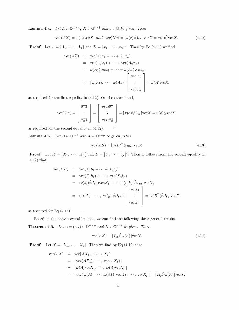
Lemma 4.4. Let A ∈ Om×n, X ∈ On×1 and a ∈ O be given. Then

vec(AX) = ω(A)vecX and vec(Xa) = [ ν(a)⊗I8n ]vecX = ν(a)⊗vecX. (4.12)

Proof. Let A = [ A1, · · · , An ] and X = [ x1, · · · , xn ]T . Then by Eq.(4.11) we find

vec(AX) = vec(A1x1 + · · · + Anxn)

= vec(A1x1) + · · · + vec(Anxn)

= ω(A1)vecx1 + · · · + ω(An)vecxn

= [ ω(A1), · · · , ω(An) ]

vecx1

...

vecxn

= ω(A)vecX,

as required for the first equality in (4.12). On the other hand,

vec(Xa) =

−→x1a...

−−→xna

=

ν(a)−→x1

...

ν(a)−→xn

= [ ν(a)⊗I8n ]vecX = ν(a)⊗vecX,

as required for the second equality in (4.12). 2

Lemma 4.5. Let B ∈ Op×1 and X ∈ On×p be given. Then

vec (XB) = [ ν(BT )⊗I8n ]vecX. (4.13)

Proof. Let X = [ X1, · · · , Xp ] and B = [ b1, · · · , bp ]T . Then it follows from the second equality in

(4.12) that

vec(XB) = vec(X1b1 + · · · + Xpbp)

= vec(X1b1) + · · · + vec(Xpbp)

= (ν(b1)⊗I8n)vecX1 + · · · + (ν(bp)⊗I8n)vecXp

= ( [ ν(b1), · · · , ν(bp) ]⊗I8n )

vecX1

...

vecXp

= [ν(BT )⊗I8n]vecX,


Based on the above several lemmas, we can find the following three general results.

Theorem 4.6. Let A = (ast) ∈ Om×n and X ∈ On×p be given. Then

vec(AX) = [ I8p⊗ω(A) ]vecX. (4.14)

Proof. Let X = [ X1, · · · , Xp ]. Then we find by Eq.(4.12) that

vec(AX) = vec[ AX1, · · · , AXp ]

= [ vec(AX1), · · · , vec(AXp) ]

= [ ω(A)vecX1, · · · , ω(A)vecXp ]

= diag(ω(A), · · · , ω(A) )[ vecX1, · · · , vecXp ] = [ I8p⊗ω(A) ]vecX,

15

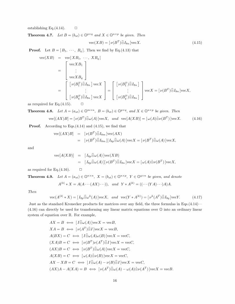
establishing Eq.(4.14). 2

Theorem 4.7. Let B = (bst) ∈ Op×q and X ∈ O

n×p be given. Then

vec(XB) = [ ν(BT )⊗I8n ]vecX. (4.15)

Proof. Let B = [ B1, · · · , Bq ]. Then we find by Eq.(4.13) that

vec(XB) = vec[ XB1, · · · , XBq ]

=

vecXB1

...

vecXBq

=

[ν(BT

1 )⊗I8n

]vecX

...[ν(BT

q )⊗I8n

]vecX

=

[ν(BT

1 )⊗I8n

]

...[ν(BT

q )⊗I8n

]

vecX = [ ν(BT )⊗I8n ]vecX,

as rerquired for Eq.(4.15). 2

Theorem 4.8. Let A = (ast) ∈ Om×n, B = (bst) ∈ Op×q, and X ∈ On×p be given. Then

vec[(AX)B] = [ ν(BT )⊗ω(A) ]vecX, and vec[A(XB)] = [ ω(A)⊗ν(BT ) ]vecX. (4.16)

Proof. According to Eqs.(4.14) and (4.15), we find that

vec[(AX)B] = [ ν(BT )⊗I8m ]vec(AX)

= [ ν(BT )⊗I8m ][ I8p⊗ω(A) ]vecX = [ ν(BT )⊗ω(A) ]vecX,

and

vec[A(XB)] = [ I8p⊗ω(A) ]vec(XB)

= [ I8p⊗ω(A) ][ ν(BT )⊗I8n ]vecX = [ ω(A)⊗ν(BT ) ]vecX,


Theorem 4.9. Let A = (ast) ∈ On×n, X = (bst) ∈ On×p, Y ∈ Oq×n be given, and denote

A(k| ∗ X = A(A · · · (AX) · · ·)), and Y ∗ A|k) = ((· · · (Y A) · · ·)A)A.

Then

vec(A(k| ∗ X) = [ I8p⊗ωk(A) ]vecX, and vec(Y ∗ A|k)) = [ νk(AT )⊗I8q ]vecY. (4.17)

Just as the standard Kronecker products for matrices over any field, the three formulas in Eqs.(4.14)—

(4.16) can directly be used for transforming any linear matrix equations over O into an ordinary linear

system of equation over R. For example,

AX = B ⇐⇒ [ I⊗ω(A) ]vecX = vecB,

XA = B ⇐⇒ [ ν(AT )⊗I ]vecX = vecB,

A(BX) = C ⇐⇒ [ I⊗ω(A)ω(B) ]vecX = vecC,

(XA)B = C ⇐⇒ [ ν(BT )ν(AT )⊗I ]vecX = vecC,

(AX)B = C ⇐⇒ [ ν(BT )⊗ω(A) ]vecX = vecC,

A(XB) = C ⇐⇒ [ ω(A)⊗ν(B) ]vecX = vecC,

AX − XB = C ⇐⇒ [ I⊗ω(A) − ν(B)⊗I ]vecX = vecC,

(AX)A − A(XA) = B ⇐⇒ [ ν(AT )⊗ω(A) − ω(A)⊗ν(AT ) ]vecX = vecB.

16

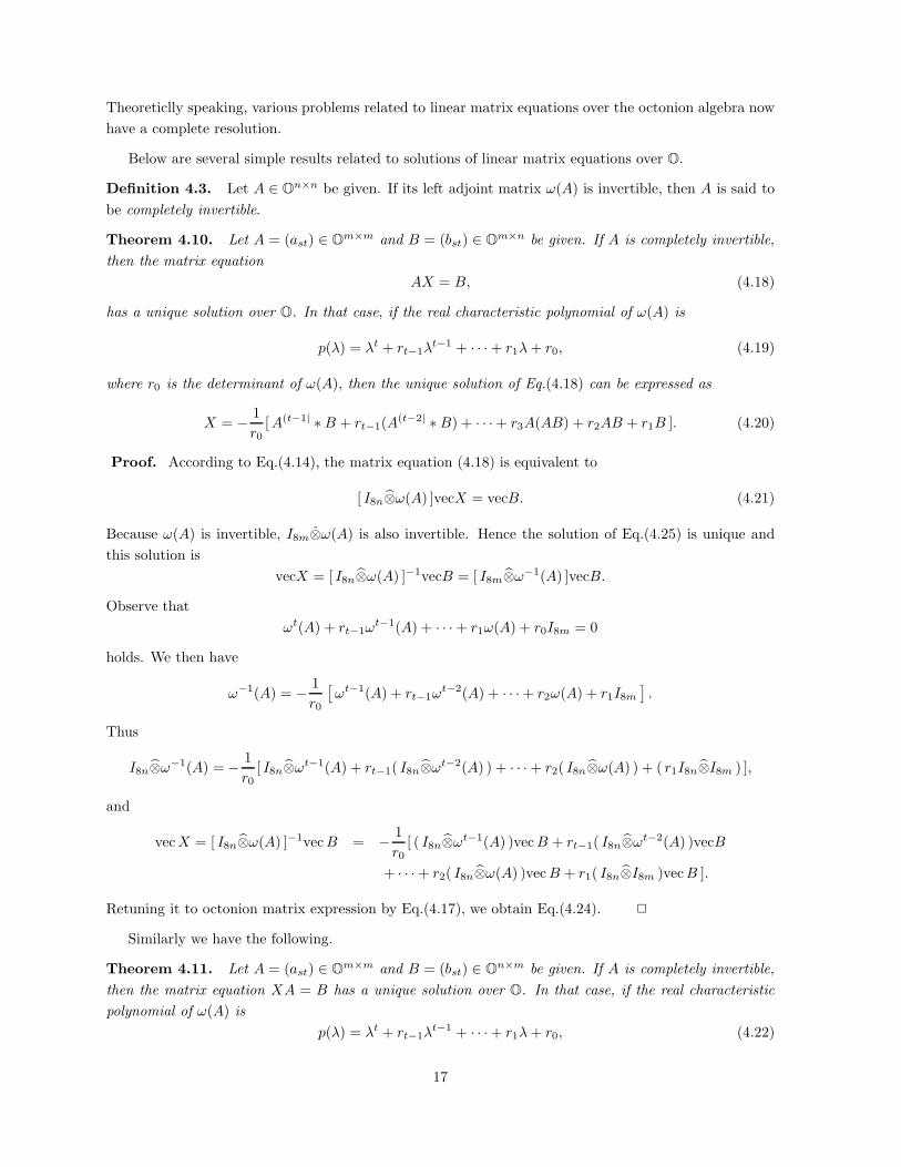
Theoreticlly speaking, various problems related to linear matrix equations over the octonion algebra now

have a complete resolution.

Below are several simple results related to solutions of linear matrix equations over O.

Definition 4.3. Let A ∈ On×n be given. If its left adjoint matrix ω(A) is invertible, then A is said to

be completely invertible.

Theorem 4.10. Let A = (ast) ∈ Om×m and B = (bst) ∈ Om×n be given. If A is completely invertible,

then the matrix equation

AX = B, (4.18)

has a unique solution over O. In that case, if the real characteristic polynomial of ω(A) is

p(λ) = λt + rt−1λt−1 + · · · + r1λ + r0, (4.19)

where r0 is the determinant of ω(A), then the unique solution of Eq.(4.18) can be expressed as

X = − 1

r0[ A(t−1| ∗ B + rt−1(A

(t−2| ∗ B) + · · · + r3A(AB) + r2AB + r1B ]. (4.20)

Proof. According to Eq.(4.14), the matrix equation (4.18) is equivalent to

[ I8n⊗ω(A) ]vecX = vecB. (4.21)

Because ω(A) is invertible, I8m⊗ω(A) is also invertible. Hence the solution of Eq.(4.25) is unique and

this solution is

vecX = [ I8n⊗ω(A) ]−1vecB = [ I8m⊗ω−1(A) ]vecB.

Observe that

ωt(A) + rt−1ωt−1(A) + · · · + r1ω(A) + r0I8m = 0

holds. We then have

ω−1(A) = − 1

r0

[ωt−1(A) + rt−1ω

t−2(A) + · · · + r2ω(A) + r1I8m

].

Thus

I8n⊗ω−1(A) = − 1

r0[ I8n⊗ωt−1(A) + rt−1( I8n⊗ωt−2(A) ) + · · · + r2( I8n⊗ω(A) ) + ( r1I8n⊗I8m ) ],

and

vecX = [ I8n⊗ω(A) ]−1vec B = − 1

r0[ ( I8n⊗ωt−1(A) )vec B + rt−1( I8n⊗ωt−2(A) )vecB

+ · · · + r2( I8n⊗ω(A) )vec B + r1( I8n⊗I8m )vecB ].

Retuning it to octonion matrix expression by Eq.(4.17), we obtain Eq.(4.24). 2

Similarly we have the following.

Theorem 4.11. Let A = (ast) ∈ Om×m and B = (bst) ∈ On×m be given. If A is completely invertible,

then the matrix equation XA = B has a unique solution over O. In that case, if the real characteristic

polynomial of ω(A) is

p(λ) = λt + rt−1λt−1 + · · · + r1λ + r0, (4.22)

17

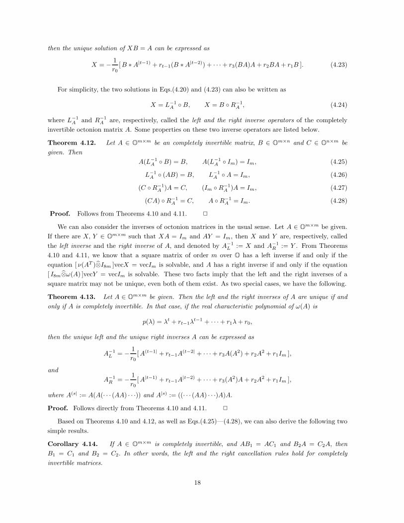
then the unique solution of XB = A can be expressed as

X = − 1

r0[ B ∗ A|t−1) + rt−1(B ∗ A|t−2)) + · · · + r3(BA)A + r2BA + r1B ]. (4.23)

For simplicity, the two solutions in Eqs.(4.20) and (4.23) can also be written as

X = L−1A ◦ B, X = B ◦ R−1

A , (4.24)

where L−1A and R−1

A are, respectively, called the left and the right inverse operators of the completely

invertible octonion matrix A. Some properties on these two inverse operators are listed below.

Theorem 4.12. Let A ∈ Om×m be an completely invertible matrix, B ∈ Om×n and C ∈ On×m be

given. Then

A(L−1A ◦ B) = B, A(L−1

A ◦ Im) = Im, (4.25)

L−1A ◦ (AB) = B, L−1

A ◦ A = Im, (4.26)

(C ◦ R−1A )A = C, (Im ◦ R−1

A )A = Im, (4.27)

(CA) ◦ R−1A = C, A ◦ R−1

A = Im. (4.28)

Proof. Follows from Theorems 4.10 and 4.11. 2

We can also consider the inverses of octonion matrices in the usual sense. Let A ∈ Om×m be given.

If there are X, Y ∈ Om×m such that XA = Im and AY = Im, then X and Y are, respectively, called

the left inverse and the right inverse of A, and denoted by A−1L := X and A−1

R := Y . From Theorems

4.10 and 4.11, we know that a square matrix of order m over O has a left inverse if and only if the

equation [ ν(AT )⊗I8m ]vecX = vecIm is solvable, and A has a right inverse if and only if the equation

[ I8m⊗ω(A) ]vecY = vecIm is solvable. These two facts imply that the left and the right inverses of a

square matrix may not be unique, even both of them exist. As two special cases, we have the following.

Theorem 4.13. Let A ∈ Om×m be given. Then the left and the right inverses of A are unique if and

only if A is completely invertible. In that case, if the real characteristic polynomial of ω(A) is

p(λ) = λt + rt−1λt−1 + · · · + r1λ + r0,

then the unique left and the unique right inverses A can be expressed as

A−1L = − 1

r0[ A(t−1| + rt−1A

(t−2| + · · · + r3A(A2) + r2A2 + r1Im ],

and

A−1R = − 1

r0[ A|t−1) + rt−1A

|t−2) + · · · + r3(A2)A + r2A

2 + r1Im ],

where A(s| := A(A(· · · (AA) · · ·)) and A|s) := ((· · · (AA) · · ·)A)A.

Proof. Follows directly from Theorems 4.10 and 4.11. 2

Based on Theorems 4.10 and 4.12, as well as Eqs.(4.25)—(4.28), we can also derive the following two

simple results.

Corollary 4.14. If A ∈ Om×m is completely invertible, and AB1 = AC1 and B2A = C2A, then

B1 = C1 and B2 = C2. In other words, the left and the right cancellation rules hold for completely

invertible matrices.

18

Corollary 4.15. Suppose that A ∈ Om×m, B ∈ On×n are completely invertible and C ∈ Om×n. Then

(a) The matrix equation A(XB) = C has a unique solution X = (L−1A ◦ C)R−1

B .

(b) The matrix equation (AX)B = C has a unique solution X = L−1A (C ◦ R−1

B ),

where L−1A and R−1

B are the left and the right inverse operators of A and B respectively.

Our next result is concerned with the extension of the Cayley-Hamilton theorem to octonion matrices,

which could be regarded as one of most successful applications of matrix representations of octonions.

Theorem 4.16. Let A ∈ Om×m be given and suppose that the real characteristic polynomial of ω(A) is

p(λ) = λt + rt−1λt−1 + · · · + r1λ + r0.

Then A satisfies the following two identities

A(t| + rt−1A(t−1| + · · · + r3A(AA) + r2A

2 + r1A + r0Im = 0, (4.29)

A|t) + rt−1A|t−1) + · · · + r3(AA)A + r2A

2 + r1A + r0Im = 0. (4.30)

Proof. Observe that p[ω(A)] = 0. It follows that

[ I8m⊗p[ω(A)] ]vecIm = 0. (4.31)

On the other hand, it is east to see by Eq.(4.17) that

vecA(s| = vec(A(s| ∗ Im) = [ I8m⊗ωs(A) ]vecIm, s = 1, 2, · · · .

Thus we find that

[ I8m⊗p(ω(A)) ]vec Im

= [ I8m⊗ωt(A) + rt−1( I8m⊗ωt−1(A) ) + · · · + r1( I8m⊗ω(A) ) + r0( I8m⊗I8m ) ]vec Im

= ( I8m⊗ωt(A) )vecIm + rt−1( I8m⊗ωt−1(A) )vec Im + · · · + r1( I8m⊗ω(A) )vec Im + r0( I8m⊗I8m )vec Im

= vecA(t| + rt−1vecA(t−1| + · · · + r1vecA + r0vec Im

= vec[ A(t| + rt−1A(t−1| + · · · + r1A + r0Im ].

The combination of this equality with Eq.(4.31) results in Eq.(4.29). The identity in Eq.(3.30) can be

established similarly. 2

Finally we present a result on real eigenvalues of Hermitian octonion matrices.

Theorem 4.17. Suppose that A ∈ Om×m is Hermitian, that is, A∗ = A. Then A and its real adjoint

ω(A) have identical real eigenvalues.

Proof. Since A = A∗, we know by Theorem 4.1(e) that ω(A) = ω(A∗) = ωT (A), that is, ω(A) is a

real symmetric matrix. In that case, all eigenvalues of ω(A) are real. Now suppose that

ω(A)X = Xλ, (4.32)

where λ ∈ R and X ∈ R8m×1. Then there is unique Y ∈ Om×1 such that vec Y = X . In that case, it is

easy to find by Theorem 4.1(a) and Eq.(4.12) that

ω(A)X = Xλ =⇒ ω(A)vec Y = vec Y λ =⇒ vec (AY ) = vec (Y λ) =⇒ AY = Y λ, (4.33)

19

which implies that λ is a real eigenvalue of A, and Y is a eigenvector of A corresponding to this λ.

Conversely suppose that AY = Y λ, where λ ∈ R, Y ∈ Om×1. Then taking vec operation on its both

sides according to Eq.(4.12) yields

ω(A)vec Y = vecY λ.

This implies that λ is also a real eigenvalue of ω(A) and vecY is a real eigenvector of ω(A) associcated

with this λ. 2

The above result clearly shows that real eigenvalues and the corresponding eigenvectors of a Hermitian

octonion matrix A can all be determined by its real adjoint ω(A). Since ω(A) is a real symmetric 8m×8m

matrix, it has 8m eigenvalues and 8m corresponding orthogonal eigenvectors.

Now a fundamental problem would naturally be asked: how many different real eigenvalues can a

Hermitian octonion matrix A have at most? For a 2×2 Hermitian octonion matrix A =

[a b

b c

], where

a, c ∈ R, its real adjoint is

ω(A) =

[aI8 ω(b)

ωT (b) cI8

].

Clearly the characteristic polynomial of ω(A) is

det(λI16 − ω(A) ) = [ (λ − a)(λ − c) − |b|2 ]8.

This shows that ω(A), and correspondingly A, has 2 eigenvalues, each of which has a multiplicity 8.

The eigenvalue problem for 3 × 3 Hermitian octonion matrices was recently examined by Dray and

Manogue [6] and Okubo [11]. They showed by algebraic methods that every 3 × 3 Hermitian octonion

matrix has 24 real eigenvalues which are divided into 6 groups, each of them has multiplicity 4. Now

according to Theorem 4.17, the real eigenvalues of any 3 × 3 Hermitian octonion matrix

A =

a11 a12 a13

a12 a22 a23

a13 a23 a33

, a11, a22, a33 ∈ R,

can be completely determined by its real adjoint

ω(A) =

ω(a11) ω(a12) ω(a13)

ωT (a12) ω(a22) ω(a23)

ωT (a13) ωT (a23) ω(a33)

.

Obviously this matrix has 24 real eigenvalues and the 24 corresponding real orthogonal eigenvectors.

Numerical computation shows that these 24 eigenvalues are divided into 6 groups, each of them has

multiplicity 4, which is consistent with the fact revealed in [6] and [11]. Moreover the 24 real orthogonal

eigenvectors can also be converted to octonion expressions by (4.33).

Furthermore, numerical computation reveals an interesting fact that the 32 real eigenvalues any 4× 4

Hermitian octonion matrix are divided into 16 groups, each of them has multiplicity 2; the 40 real

eigenvalues of any 5×5 Hermitian octonion matrix are divided into 20 groups, each of them has multiplicity

2.

In general, we guess that for any m×m Hermitian octonion matrix with m > 3, its 8m real eigenvalues

can be divided into 4m groups, each of them has multiplicity 2.

As a subsequent work of Thereom 4.17, one might naturally ask hwo to establish a possible factor-

ization for a Hermitian octonion matrix using its real eigenvalues and corresponding octonion orthogonal

20

eigenvectors, speak more precisely, for an m×m Hermitian octonion matrix A, how construct a complete

invertible octonion matrix P (unitary?) and a real diagonal matrix D such that A = PDP−1 using

its 8m real eigenvalues and 8m corresponding octonion orthogonal eigenvectors. However, this problem

seems quite curious, because the number of different real eigenvalues of an Hermitian octonion matrix

is more than its order. This problem is also quite challenging, because various traditional methods in

associative matrix theory are not applicable to this non-associative case.

As pointed out in [6], Hermitian octonion matrices can also have non-real right eigenvalues. Theoret-

ically speaking, the non-real eigenvalue problem of Hermitian octonion matrices may also be converted

to a problem related to real representations of octonion matrices. In fact, suppose that AX = Xλ, where

λ ∈ O and X ∈ Om×1. Then according to Eq.(4.12), it is equivalent to

ω(A)vec X = ν(λ)⊗vecX,

or alternatively

[ ω(A) − diag( ν(λ), · · · , ν(λ) ]vec X = 0.

How to find ν(λ) satisfying the equation remains to further study.

Conclusions. In this paper, we have introduced two pseudo real matrix representations for octonions.

Based on them we have made a complete investigation to their operation properties and have considered

their various applications to octonions and matrices of octonions. However our work could only be

regarded as a first step in the research of octonion matrix analysis and its applications. Numerous

problems related to matrices of octonions remain to further examine, such as:

(a) How to determine eigenvalues and eigenvectors of a square octonion matrix, not necessarily Hermi-

tian, and what is the relationship of eigenvalues and eigenvectors of a octonion matrix and its real

adjoint matrices?

(b) Besides Eq.(4.29) and (4.30), how to establish some other identities for octonion matrices through

their adjoint matrices?

(c) How to establish similarity theory for octonion matrices, and how to determine the relationship

between the similarity of octonions matrices and the similarity of their adjoint matrices?

(d) How to consider various possible decompositions of octonion matrices, such as, LU decomposition,

singular value decomposition and Schur decomposition?

(e) How to characterize various particular octonion matrices, such as, idempotent matrices, nipoltent

matrices, involutary matrices, unitary matrices, normal matrices, and so on?

(f) How to define generalized inverses of octonion matrices when they are not completely invertible?

and so on. As mentioned in the beginning of the section, matrix multiplication for octonion matrices is

completely not associative. In that case, any further research to problems related matrices of octonions

is extremely difficult, but is also quite challenging. Any advance in solving the problems mentioned

above could lead to remarkable new development in the real octonion algebra and its applications in

mathematical physics.

Finally we should point out that the results obtained in the paper can use to establish pseudo matrix

representations for real sedenions, as well as, in general, for elements in any 2n-dimensional real Cayley-

Dickson algebras.

21

References

[1] J. L. Brenner, Matrices of quaternions, Pacific J. Math. 1(1951), 329–335.

[2] P. M. Cohn, The range of the derivation and the equation ax − xb = c, J. Indian Math. Soc. 37(1973), 1–9.

[3] P. M. Cohn, Skew Field Constructions, Cambridge U. P., London, 1977.

[4] P. J. Daboul and R. Delbourgo, Matrix representation of octonions and generalizations, J. Math. Phys. 40

(1999), 4134-4150.

[5] G. M. Dixon, Division algebras: octonions, quaternions, complex numbers and the algebraic design of physics,

Mathematics and its Applications 290. Kluwer Academic Publishers Group, Dordrecht, 1994.

[6] T. Dray and C. A. Manogue, The octonionic eigenvalue problem, Adv. Appl. Clifford Algebras 8(1998),

341–364.

[7] H. C. Lee, Eigenvalues of canonical forms of matrices with quaternion coefficients, Proc. Roy. Irish. Acad.

Sect. A 52(1949), 253-260.

[8] R. E. Johnson, On the equation χα = γχ+β over an algebraic division ring, Bull. Amer. Math. Soc. 50(1944),

202–207.

[9] O. V. Ogievetskiı, A characteristic equation for 3 × 3 matrices over the octonions. (Russian) Uspekhi Mat.

Nauk 36(1981), 197–198.

[10] S. Okubo, Introduction to octonion and other non-associative algebras in physics, Montroll Memorial Lecture

Series in Mathematical Physics, 2. Cambridge University Press, Cambridge, 1995.

[11] S. Okubo, Eigenvalue problem for symmetric 3 × 3 octonionic matrix Adv. Appl. Clifford Algebras 9(1999),

131–176.

[12] R. D. Schafar, An introduction to non-associative algebras, Academic Press, New York, 1966.

[13] Y. Tian, Universal factorization equalities over real Clifford algebras, Adv. Appl. Clifford Algebras 8(1998),

365–402.

[14] Y. Tian, Similarity and consimilarity of elements in the real Cayley-Dickson algebras Adv. Appl. Clifford

Algebras 9(1999), 61–76.

[15] N. A. Wiegmann, Some theorems on matrices with real quaternion elements, Canad. J. Math. 7(1955),

191–201.

[16] L. A. Wolf, Similarity of matrices in which the elements are real quaternions, Bull. Amer. Math. Soc.

42(1936), 737–743.

[17] K. A. Zhevlakov et al, Rings that are nearly associative, Academic Press, New York, 1982.

22